sampling bias and implicit knowledge in ecological niche modelling … · dekker, sampling bias and...

Sampling Bias and Implicit Knowledge in Ecological

Niche Modelling

A. H. Dekker a

a Dekker Consulting, P.O. Box 3925, Manuka, ACT, 2603, Australia

Email: [email protected]

Abstract: Ecological niche modelling is an important method for predicting the range of a species, which

can be used to support conservation efforts and assist in biological understanding. Ecological niche

modelling relies on observations by field biologists, but these may suffer from sampling bias, due to

difficulties such as those illustrated in Figure 1.

In this paper we use synthetic species distribution data to evaluate a number of modelling mechanisms for

dealing with sampling bias in data from the field (Phillips et al. 2009; Syfert et al. 2013; Kramer-Schadt, et

al. 2013), and we simulate a modeller attempting to reconstruct the distribution from that data. Synthetic data

lets us assess the modeller’s work against “ground truth.” The modeller typically uses a machine learning

algorithm like Maxent or Random Forests, together with ‘presence’ datapoints from field biologists and

randomly generated ‘background’ datapoints. We consider bias in general terms, rather than simulating a

specific bias mechanism. Figure 2 shows the ecological niche modelling process we have simulated.

Our results show that, in cases of sampling bias, the Maxent algorithm generally performs as well as or better

than Random Forests. Where the field biologists have concentrated their sampling efforts in a specific ‘focus

area,’ there is generally a benefit in a ‘boost’ of additional ‘background’ datapoints within that area. Using

implicit biological knowledge to exclude ‘impossible’ regions from the study area has mixed effects. Spatial

filtering, as suggested by Kramer-Schadt, et al. (2013), may sometimes have significant negative effects.

Our results also show that, where sampling bias occurs, AUC scores are a poor guide to true algorithm

performance (although, without knowledge of the true distribution, it is generally the best available guide).

Figure 1. Sampling difficulties: vegetation (horizontal scrub, Anodopetalum biglandulosum, in Tasmania –

photo by Phillip Hirst, 2010), terrain (highlands of Papau New Guinea – photo by eGuide Travel, 2010), and

distance from roads (Sahara desert, Kebili, Tunisia – photo by “wonker,” 2010). Images from

www.flickr.com/photos/{phil_hirst/4310391447,eguidetravel/5986605253,wonker/4300464711}.

Figure 2. The process of ecological niche modelling, which we study in this paper.

Keywords: Ecological niche modelling, Species distribution modelling, Sampling bias, Maxent

22nd International Congress on Modelling and Simulation, Hobart, Tasmania, Australia, 3 to 8 December 2017 mssanz.org.au/modsim2017

922

mailto:[email protected]

Dekker, Sampling Bias and Implicit Knowledge in Ecological Niche Modelling

1. INTRODUCTION

The niche modelling process is shown in Figure 2. We will use the term “zumbat” for a fictional species, and

write p(t, x, y) for the probability of finding a zumbat at position (x, y) at time t. At ‘presence’ points where

biologists have found a zumbat, ∃ t. p(t, x, y) = 1. Elsewhere, ∀ t. p(t, x, y) < 1. Usually, we are interested in

integrating over time, i.e. p(x, y) = ∫t p(t, x, y). At ‘presence’ points p(x, y) > 0, with p(x, y) < 1 elsewhere.

Machine learning algorithms such as Maxent (Phillips et al., 2006; Elith et al., 2011) and Random Forests

(Breiman, 2001) are typically used. These require both ‘presence’ and ‘absence’ data, and so we provide

input data p(x, y) = 1 for ‘presence’ points and p(x, y) = 0 for a random set of ‘background’ or ‘pseudo-

absence’ points. Figure 3(a,b,c) shows a synthetic species distribution p(x, y) with some random ‘presence’

points, while Figure 3(d) shows a distribution inferred by machine learning.

This paper studies sampling bias in data collected by the field biologist, which is often as a result of access

difficulties. Some areas may be under-surveyed because of vegetation, terrain, or general isolation (Figure 1).

Resource constraints also have an effect. A country’s ability to conduct area-related activities can be

estimated by its GDP per sq km. Well-resourced countries include the UK ($11M per sq km) and the

Netherlands ($19M). However, large sparsely-populated countries such as Australia ($0.16M) and Canada

($0.15M) rank about the same as developing countries like Cambodia ($0.11M) and Nepal ($0.14M).

2. EXPERIMENT 1 – METHODS

Our study area is a region of eastern Australia bounded by 140°E to 154°E longitude and 22°S to 36°S

latitude. For the experiments reported here, we use three artificial species distributions, shown in Figure

3(a,e,f). For each distribution, p(x,y) = α(x,y) β(x,y) γ(x,y). Here α(x,y) = (φ(x,y) − a)2

(φ(x,y) − b)2 for a ≤

φ(x,y) ≤ b, where a and b are arbitrary limits and φ(x,y) is one of the first four principal components resulting

from principal components analysis of the 19 WorldClim “bioclimatic variables” in the WorldClim database

at worldclim.org (Hijmans et al., 2005). The “bioclimatic variables” are at 30-second resolution. As in Pie et

al. (2013), we use the principal components of these bioclimatic variables in order to avoid the problem of

correlated variables. We have α(x,y) = 0 for φ(x,y) < a or φ(x,y) > b. The component β(x,y) is defined

similarly to α, but for a different principal component. The pairs of principal components used for α and β are

1–2, 1–3, and 2–4 (these were chosen so that the corresponding species distribution zones A, B, and C would

vary in size and shape). The component γ(x,y) takes human disturbance into account using NASA imagery of

the earth at night. We define γ(x,y) = 1 for the darkest (least disturbed) areas and γ(x,y) = 0 for the brightest

(urban) areas, interpolating linearly between those extremes (a more complete measure of human disturbance

would be the Human Footprint maps of Venter et al., 2016).

For each of the zones (A, B, and C) of artificial species distribution in Figure 3(a,e,f), we randomly generate

a set of 100 ‘presence’ datapoints with probability proportional to p(x,y). Figure 3(a) illustrates an example.

We also introduce partial and full sampling bias options. Both are based on a focus area which for

experimental purposes is taken to be a circle of radius 200 km (in reality, of course, the focus area would be

an irregular region determined by the geographical factors illustrated in Figure 1). With partial sampling bias,

the probability of ‘presence’ datapoints is four times greater within the circle than outside. With full

sampling bias, ‘presence’ datapoints are chosen only from inside the circle. Figure 3(a,b,c) shows examples

of no bias, partial bias, and full bias. For zone A, the focus area covers a relatively small part of a large

distribution. For zone B, the focus area covers roughly the southern half of the distribution. For zone C,

almost the entire distribution is within the focus area, so that very little real bias is actually occurring.

As usual, the ‘presence’ datapoints are combined with a set of randomly generated ‘background’ datapoints

(Wisz et al. 2008). Our simulated modeller generates 800 of these, chosen to be at least 10 km from the

‘presence’ datapoints. Because generating ‘background’ datapoints is an activity carried out by the modeller,

it applies to the entire study area and is independent of p(x,y). Figure 3(d) shows an example of machine

learning output for zone A with full bias.

Our simulated modeller attempts to reconstruct the species p(x,y) using both the Maxent (Phillips et al.,

2006; Elith et al., 2011) and Random Forests (Breiman, 2001) algorithms, which we have used in previous

work (Dekker and Rowley, 2015). In addition, we explore the impact of a background datapoint boost,

which produces more ‘background’ datapoints within the focus area. This ‘boost’ generates a minimum of

200 ‘background’ datapoints within the focus area, followed by an additional 600 across the whole study area

(giving the same total of 800 background datapoints). We used the R software toolkit (version 3.2.4) with the

“raster” (version 2.5-2), “randomForest” (version 4.6-12), and “dismo” (version 1.0-15) packages (Hijmans

and Elith, 2015). The latter was interfaced to version 3.3.3k of the Maxent program. Covariates used by the

simulated modeller were the first ten principal components of the 19 WorldClim “bioclimatic variables.” The

experiment was run 15 times, with new ‘presence’ and ‘background’ points each time.

923


As an independent measure of performance for the two machine learning algorithms, we used the correlation

between the true probability p(x,y) and the inferred probability from machine learning. The correlation

between the two probabilities was calculated using quadratic regression, since Dekker and Rowley (2015)

suggests a nonlinear relationship between the two probabilities. Correlations were compared using paired t-

tests. As an ‘internal’ measure of model quality, we also calculated the area under the Receiver Operating

Characteristic curve, or AUC value (Wisz et al., 2008), using independent test data (i.e. new sets of randomly

generated ‘presence’ and ‘background’ points). The median AUC value over 11 sets of test data was used.

In a supplementary experiment, we follow the suggestion of Kramer-Schadt, et al. (2013) to undo bias by

randomly deleting excess ‘presence’ datapoints within the focus area. This restores an unbiased sampling

probability, but reduces the sample size. It only makes sense to do so for zones A and B with partial bias.

(a) Zone A, no sampling bias. (b) Zone A, partial sampling bias.

(c) Zone A, full sampling bias. (d) Reconstructed distribution for zone A (Maxent).

(e) Zone B, full bias. (f) Zone C, full bias.

Figure 3. Artificial species distributions A, B, and C, showing three sampling bias options for zone A (all

three options were also applied to zones B and C, but are omitted here for space reasons). The colour scale

shows probability p(x,y), with white = 0 and red = 1. Black circles show ‘presence’ datapoints, which are

generated randomly with probability proportional to p(x,y), with possible sampling bias.

924


3. EXPERIMENT 1 – RESULTS AND DISCUSSION

Figure 4 shows the results of the first experiment, averaged over 15 runs. Assessing statistical significance at

the 1% level, in the unbiased case, Maxent outperforms Random Forests only for zone A (a correlation of

0.94 vs 0.88). In the biased case, Maxent outperforms Random Forests for six cases:

zone A with partial bias (0.92 vs 0.85 for background boost, 0.91 vs 0.84 for no boost);

zone A with full bias, which is not surprisingly the worst case (0.61 vs 0.56 for background boost,

0.50 vs 0.47 for no boost); and

zone B with partial bias (0.91 vs 0.89 for background boost, 0.88 vs 0.86 for no boost).

Random Forests very slightly outperform Maxent for zone C with full bias and no background boost (0.88 vs

0.87) although, with a statistical significance barely meeting the 1% criterion (actually, 0.7%), this is

probably a chance effect.

Because of the simplicity of the synthetic distribution p(x,y) = α(x,y) β(x,y) γ(x,y) we have used, it is possible

that our results are slightly biased in favour of Maxent, which may infer simpler models than Random

Forests. However, this property of Maxent is often desirable for real-world data (Dekker and Rowley, 2015).

The use of background boost has a positive effect for all cases of bias except zone A with partial bias:

zone A with full bias (0.56 vs 0.47 for RF, 0.61 vs 0.50 for Maxent);

zone B with full bias (0.79 vs 0.76 for RF, 0.82 vs 0.76 for Maxent);

zone B with partial bias (0.89 vs 0.86 for RF, 0.91 vs 0.88 for Maxent);

zone C with full bias (0.90 vs 0.88 for RF, 0.91 vs 0.87 for Maxent); and

zone C with partial bias only for Maxent (0.91 vs 0.87).

The stronger effect of background boost with full bias is consistent with Phillips et al. (2009) and Syfert et al.

(2013). However, the benefit of background boost even for zone C, where there is little real bias, suggests

that there is also a benefit in having more background points closer to the ‘presence’ points even when there

is no actual sampling bias (thus allowing machine learning to better discriminate presence vs absence).

Figure 4. Results of the 1st experiment. Here ‘RF’ refers to Random Forests, and ‘+’ to the use of a

background boost. Error bars show minimum and maximum results over 15 runs.

As Figure 5 shows, there was essentially no relationship between the commonly used AUC score and the

correlation used as a measure of performance. This implies that, where sampling bias occurs, AUC scores are

a poor guide to algorithm performance. Because AUC scores are an ‘internal’ measure (measuring the fit to

the sample data), they can be very high even when true performance (as measured by the correlation) is low.

For the supplementary experiment (removing bias by deleting excess ‘presence’ datapoints), which we

conducted only with Maxent and partial bias, we obtained a correlation (between true and inferred

probabilities) of 0.94 for zone A. At the 1% level, this is a statistically significant improvement on Maxent

alone (0.91) or Maxent with background boost (0.92). However, for zone B, we obtained a correlation of only

0.78, which is significantly worse than Maxent alone (0.88) or Maxent with background boost (0.91).

925


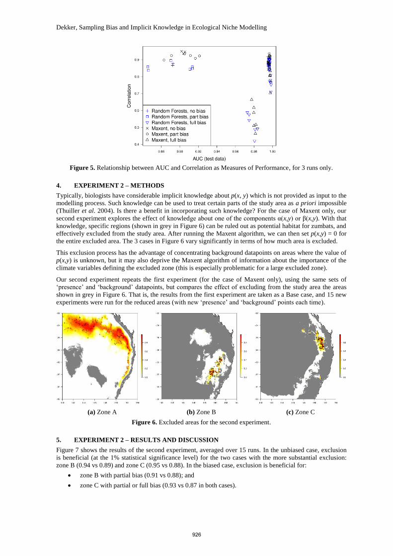
Figure 5. Relationship between AUC and Correlation as Measures of Performance, for 3 runs only.

4. EXPERIMENT 2 – METHODS

Typically, biologists have considerable implicit knowledge about p(x, y) which is not provided as input to the

modelling process. Such knowledge can be used to treat certain parts of the study area as a priori impossible

(Thuiller et al. 2004). Is there a benefit in incorporating such knowledge? For the case of Maxent only, our

second experiment explores the effect of knowledge about one of the components α(x,y) or β(x,y). With that

knowledge, specific regions (shown in grey in Figure 6) can be ruled out as potential habitat for zumbats, and

effectively excluded from the study area. After running the Maxent algorithm, we can then set p(x,y) = 0 for

the entire excluded area. The 3 cases in Figure 6 vary significantly in terms of how much area is excluded.

This exclusion process has the advantage of concentrating background datapoints on areas where the value of

p(x,y) is unknown, but it may also deprive the Maxent algorithm of information about the importance of the

climate variables defining the excluded zone (this is especially problematic for a large excluded zone).

Our second experiment repeats the first experiment (for the case of Maxent only), using the same sets of

‘presence’ and ‘background’ datapoints, but compares the effect of excluding from the study area the areas

shown in grey in Figure 6. That is, the results from the first experiment are taken as a Base case, and 15 new

experiments were run for the reduced areas (with new ‘presence’ and ‘background’ points each time).

(a) Zone A (b) Zone B (c) Zone C

Figure 6. Excluded areas for the second experiment.

5. EXPERIMENT 2 – RESULTS AND DISCUSSION

Figure 7 shows the results of the second experiment, averaged over 15 runs. In the unbiased case, exclusion

is beneficial (at the 1% statistical significance level) for the two cases with the more substantial exclusion:

zone B (0.94 vs 0.89) and zone C (0.95 vs 0.88). In the biased case, exclusion is beneficial for:

zone B with partial bias (0.91 vs 0.88); and

zone C with partial or full bias (0.93 vs 0.87 in both cases).

926


Figure 8. Location data for the thorny devil,

Moloch horridus, in part of South Australia, with

sealed and unsealed roads marked in red. Of these

locations, 79% are at most 1 km from a road.

Where background boost is used, exclusion is beneficial for zone C with partial or full bias (0.93 vs 0.91 in

both cases) but has a negative effect for zone B with full bias (0.77 vs 0.82). The latter effect is highly

significant (0.00025%). The use of exclusion is therefore obviously no panacea.

Conversely, where the grey areas in Figure 6 are excluded, background boost is beneficial for all cases except

zone C with full bias, where it has no effect.

Combining the results of the two experiments, the safe option in cases of bias appears to be Maxent with

background boost (pink bars in Figure 7), while benefits for excluding parts of the study area are mixed.

Figure 7. Results of the 2nd

experiment. Here ‘Base’ refers to the Maxent data in Figure 4, and ‘Reduced’ to

the effect of excluding the grey areas in Figure 6. As before, ‘+’ refers to the use of a background boost.

Error bars show minima and maxima over 15 runs.

6. CONCLUSIONS AND FURTHER WORK

In cases of sampling bias, our results show a benefit for using the Maxent algorithm with a boost of more

‘background’ datapoints within what we have called the focus area. But what is the focus area? Our

experiments have taken it to be a simple circle, but with real data, the focus area can be difficult to infer,

since it may correlate with climatic variables. For example, the presence of vegetation like Anodopetalum

biglandulosum (Figure 1) may correlate with high rainfall; mountainous terrain may correlate with low

temperatures; and the absence of roads may

correlate with a desert climate.

In some cases, the field biologists will be able to

explicitly describe their sampling strategy, while in

others the strategy may be obvious. For example,

Figure 8 shows location data for the thorny devil,

Moloch horridus, in part of South Australia (ALA,

2016), compared to sealed and unsealed roads in a

state database (SA Government, 2016). Of the

locations, 79% are 1 km or less from a road, while

others appear to be located on tracks not in the

database. For this set of location data, the focus area

can be taken to consist of pixels on, or adjacent to,

roads.

In other cases, a plausible focus area can be

identified from occurrence records for other species

that have been observed in the same general area

using similar methods, as suggested by Phillips et

al. (2009).

Kramer-Schadt, et al. (2013) suggest that spatial

filtering (discarding excess ‘presence’ datapoints) is

preferable to the use of background boost, but this

927


presupposes that ‘presence’ datapoints do cover the true species range, being merely denser within the focus

area (i.e. what we have called partial bias), and that there are sufficient ‘presence’ datapoints that the excess

can be discarded. Our results (in the supplementary experiment) do not support their suggestion; spatial

filtering gives a slight improvement (0.94 vs 0.92) for zone A, but a considerable degradation (0.78 vs 0.91)

for zone B. However, further work would be needed to explore this in detail.

In future work, we intend to explore these options with a greater degree of realism by using more biologically

plausible distributions for the fictional species, and by using a more realistic model of a field biologist

collecting observations. Specifically, we intend to use an explicit agent-based model of a field biologist

traversing a road network like the one in Figure 8 while collecting observations.

REFERENCES

ALA (2016). Atlas of Living Australia occurrence download for Moloch horridus at biocache.ala.org.au/

occurrences/search?&q=lsid:urn:lsid:biodiversity.org.au:afd.taxon:aa2746a5-6b1b-49e9-84d2-

9ee9b3aefe5c accessed 22 Oct 2016.

Breiman, L. (2001). Random Forests. Machine Learning, 45(1), 5-32.

Dekker, A. H. and Rowley, J.J.L. (2015). Evaluating Ecological Niche Modelling Techniques. MODSIM

2015, 21st International Congress on Modelling and Simulation. Modelling and Simulation Society of

Australia and New Zealand. 152–158. Available at www.mssanz.org.au/modsim2015/A3/dekker.pdf

Elith, J., Phillips, S.J., Hastie, T., Dudík, M., Chee, Y.E., and Yates, C.J. (2011) A statistical explanation of

MaxEnt for ecologists. Diversity and Distributions, 17, 43–57.

Hijmans, R.J., Cameron, S.E., Parra, J.L., Jones, P.G., and Jarvis, A. (2005). Very high resolution

interpolated climate surfaces for global land areas. International Journal of Climatology, 25, 1965–1978.

Hijmans, R.J. and Elith, J. (2015). Species distribution modeling with R. R project documentation, available

at cran.r-project.org/web/packages/dismo/vignettes/sdm.pdf

Kramer-Schadt, S., Niedballa, J., Pilgrim, J.D., Schroder, B., Lindenborn, J., Reinfelder, V., Stillfried, M.,

Heckmann, I., Scharf, A.K., Augeri, D.M., Cheyne, S.M., Hearn, A.J., Ross, J., Macdonald, D.W., Mathai,

J., Eaton, J., Marshall, A.J., Semiadi, G., Rustam, R., Bernard, H., Alfred, R., Samejima, H., Duckworth,

J.W., Breitenmoser-Wuersten, C., Belant, J.L., Hofer, H., and Wilting, A. (2013). The importance of

correcting for sampling bias in MaxEnt species distribution models. Diversity Distrib., 19, 1366–1379.

Phillips, S.J., Anderson, R.P., and Schapire, R.E. (2006). Maximum entropy modeling of species geographic

distributions. Ecological Modelling, 190(3–4), 231–259.

Phillips, S.J., Dudík, M., Elith, J., Graham, C.H., Lehmann, A., Leathwick, J., and Ferrier, S. (2009). Sample

selection bias and presence-only distribution models: implications for background and pseudo-absence

data. Ecological Applications. 19(1), 181–197.

Pie, M.R., Meyer, A.L.S., Firkowski, C.R., Ribeiro, L.F., and Bornschein, M.R. (2013). Understanding the

mechanisms underlying the distribution of microendemic montane frogs (Brachycephalus spp., Terrarana:

Brachycephalidae) in the Brazilian Atlantic Rainforest. Ecological Modelling. 250, 165– 176.

R Core Team (2016). R: A language and environment for statistical computing. R Foundation for Statistical

Computing (www.R-project.org), Vienna, Austria.

SA Government (2016). South Australian Statewide Road Network dataset at data.sa.gov.au/data/dataset/

roads/resource/dbd6cc0f-317e-4fc7-b734-b81a518a3f00 accessed 22 Oct 2016.

Syfert , M.M., Smith, M.J., and Coomes, D.A. (2013). The Effects of Sampling Bias and Model Complexity

on the Predictive Performance of MaxEnt Species Distribution Models. PLoS ONE, 8(2): e55158.

Thuiller, W., Brotons, L., Araújo M.B., and Lavorel, S. (2004). Effects of Restricting Environmental Range

of Data to Project Current and Future Species Distributions. Ecography, 27(2): 165–172.

Venter, O., Sanderson, E.W., Magrach, A., Allan, J.R., Beher, J., Jones, K.R., Possingham, H.P., Laurance,

W.F., Wood, P., Fekete, B.M., Levy, M.A., and Watson, J.E.M. (2016). Data Descriptor: Global terrestrial

Human Footprint maps for 1993 and 2009. Scientific Data 3:160067, doi:10.1038/sdata.2016.67.

Wisz, M.S., Hijmans, R.J., Li, J., Peterson, A.T., Graham, C.H., Guisan, A., and NCEAS Predicting Species

Distributions Working Group (2008). Effects of sample size on the performance of species distribution

models. Diversity and Distributions, 14, 763–773.

928

sampling bias and implicit knowledge in ecological niche modelling … · dekker, sampling bias and...

Documents