sample size and measurement occasion planning for latent

Running head: INSERT SHORTTITLE COMMAND IN PREAMBLE 1

Sample Size and Measurement Occasion Planning for Latent Change Score Models through

Monte Carlo Simulation

Zhiyong Zhang and Haiyan Liu

Department of Psychology, University of Notre Dame

INSERT SHORTTITLE COMMAND IN PREAMBLE 2

Abstract

Latent change score models (LCSMs) proposed by McArlde (McArdle, 2000, 2009; McArdle &

Nesselroade, 1994) offer a powerful tool for longitudinal data analysis. They are becoming

increasingly popular in the social and behavioral research (e.g., Gerstorf et al., 2007; Ghisletta &

Lindenberger, 2005; King et al., 2006; Raz et al., 2008). Although conducting both univariate and

multivariate latent change score analysis is not a difficult task any more (e.g., Ghisletta &

McArdle, 2012; Zhang et al., 2015), there is little discussion on the design issues such as sample

size planning for LCSMs. To fill the gap, this study proposes a Monte Carlo based method to

determine the required sample size and number of measurement occasions for both univariate and

bivariate LCSMs. The method can obtain the power for testing each individual parameter of the

models, especially the change rate and coupling parameters. The Monte Carlo procedure is

implemented and provided in a free R package RAMpath (Zhang et al., 2015). Examples for

sample size and measurement occasion planning for both univariate and bivariate LCSMs are

provided.


Sample Size and Measurement Occasion Planning for Latent Change Score Models through

Monte Carlo Simulation

Introduction

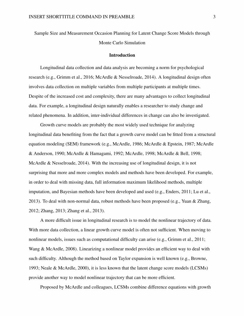
Longitudinal data collection and data analysis are becoming a norm for psychological

research (e.g., Grimm et al., 2016; McArdle & Nesselroade, 2014). A longitudinal design often

involves data collection on multiple variables from multiple participants at multiple times.

Despite of the increased cost and complexity, there are many advantages to collect longitudinal

data. For example, a longitudinal design naturally enables a researcher to study change and

related phenomena. In addition, inter-individual differences in change can also be investigated.

Growth curve models are probably the most widely used technique for analyzing

longitudinal data benefiting from the fact that a growth curve model can be fitted from a structural

equation modeling (SEM) framework (e.g., McArdle, 1986; McArdle & Epstein, 1987; McArdle

& Anderson, 1990; McArdle & Hamagami, 1992; McArdle, 1998; McArdle & Bell, 1998;

McArdle & Nesselroade, 2014). With the increasing use of longitudinal design, it is not

surprising that more and more complex models and methods have been developed. For example,

in order to deal with missing data, full information maximum likelihood methods, multiple

imputation, and Bayesian methods have been developed and used (e.g., Enders, 2011; Lu et al.,

2013). To deal with non-normal data, robust methods have been proposed (e.g., Yuan & Zhang,

2012; Zhang, 2013; Zhang et al., 2013).

A more difficult issue in longitudinal research is to model the nonlinear trajectory of data.

With more data collection, a linear growth curve model is often not sufficient. When moving to

nonlinear models, issues such as computational difficulty can arise (e.g., Grimm et al., 2011;

Wang & McArdle, 2008). Linearizing a nonlinear model provides an efficient way to deal with

such difficulty. Although the method based on Taylor expansion is well known (e.g., Browne,

1993; Neale & McArdle, 2000), it is less known that the latent change score models (LCSMs)

provide another way to model nonlinear trajectory that can be more efficient.

Proposed by McArdle and colleagues, LCSMs combine difference equations with growth


curves to study change in longitudinal studies (e.g., McArdle, 2000; McArdle & Hamagami,

2001; Hamagami & McArdle, 2007a; Hamagami et al., 2010). In such models, change is directly

modeled, which is often the focus of a longitudinal study. As we will show shortly, the models in

their nature accommodate to the nonlinear growth trajectories. In addition to the univariate

LCSMs, bivariate LCSMs have also been proposed to model the inter-relationship between two

growth processes (e.g., McArdle & Hamagami, 2001).

Fitting a LCSM in the SEM framework is easy to understand but can be tedious. It can be

done in almost any SEM software. Recently, Ghisletta & McArdle (2012) showed how to

estimate a univariate LCSM using difference R packages, including Lavaan (Rosseel, 2012),

OpenMx (Boker et al., 2011) and sem (Fox, 2006). More recently, Zhang et al. (2015) automated

the estimating procedure for the typical univariate and multivariate LCSMs through an R package

RAMpath that is developed based on RAM notations (Boker et al., 2002; McArdle & Boker,

1990).

The importance of conducting statistical power analysis at the beginning of a study is

universally accepted (e.g., Cohen, 1988; Hedges & Rhoads, 2010). Without adequate statistical

power, the validity of statistical conclusions from all kinds of research is endangered (e.g., Cohen,

1988; Hedges & Rhoads, 2010; Myors & Wolach, 2014; Shadish et al., 2002). For example,

without a carefully planned sample size, a study can easily fail to detect an existing effect by

chance and, therefore, create problems for replication or cross-validation. Although there are

studies on sample size planning and power calculation for growth curve analysis (e.g., Zhang &

Wang, 2009), we are not aware of any discussion on such design issues for LCSMs.

To fill the gap, this study proposes a Monte Carlo based method to determine the required

sample size and/or the number of measurement occasions for both univariate and bivariate

LCSMs. The method can obtain the power for testing each individual parameter of the models

such as the change rate and coupling parameters. We also implement the Monte Carlo procedure

in a free R package RAMpath (Zhang et al., 2015).

In the rest of the chapter, we first present the univariate and bivariate LCSMs. Then, we


introduce the Monte Carlo based method for power analysis. After that, we show how to conduct

power analysis for LCSMs through several examples using our developed software. We conclude

the chapter with discussion and future directions.

A Univariate Latent Change Score Model

Let Y [t]n denote the data from the nth (n = 1, . . . , N ) participant at time t (t = 1, . . . , T )

of a sample consisting of N participants measured for T times. The first part of a LCSM is a

measurement error model where an observed score Y [t]n is the sum of the latent true score y[t]n

and the measurement error/uniqueness score ey[t]n:

Y [t]n = y[t]n + ey[t]n.

It is generally assumed that the error follows a normal distribution with mean 0 and variance

varey. The second part of the model builds the relationship between consecutive latent true

scores so that the current score at time t is equal to the sum of the true score at the previous time

t− 1 and the change, dy[t]n, from time t− 1 to time t:

y[t]n = y[t− 1]n + dy[t]n.

This effectively defines the change score as

dy[t]n = y[t]n − y[t− 1]n.

Note that in the classic LCSM, the relationship between consecutive latent true scores is

deterministic although it is not required to be so. The third part of the model concerns the

modeling of the difference scores. One way is to model the difference score at time t as the sum

of a linear constant effect ys and the proportional change from time t− 1 such that

dy[t]n = ysn + βy × y[t− 1]n,

where βy is a compound rate of change.


Given the three part of the model, we can model the observed score as

Y [t]n = y[t]n + ey[t]n

= y[t− 1]n + dy[t]n + ey[t]n

= (1 + βy)y[t− 1]n + ysn + ey[t]n.

Successively expressing the above equation will lead to

Y [t]n = (1 + βy)y[t− 1]n + ysn + ey[t]n

= (1 + βy)(y[t− 2]n + dy[t− 1]n) + ysn + ey[t]n

= (1 + βy)2y[t− 2]n + (1 + βy)ysn + ysn + ey[t]n

= (1 + βy)t−1y[1]n + [1 + (1 + βy) + . . .+ (1 + βy)t−2]ysn + ey[t]n

= (1 + βy)t−1y0n + [1 + (1 + βy) + . . .+ (1 + βy)t−2]ysn + ey[t]n

where y0[n] is the initial latent score and note that the latent score at time t follows

y[t]n = (1 + βy)t−1y0n + [1 + (1 + βy) + . . .+ (1 + βy)t−2]ysn.

Clearly, the observed and latent scores behave as a nonlinear function of time and therefore can

capture the nonlinear trajectory except when βy = 0. To visually show this, we plot the latent

scores with different values for βy in Figure 1.

The initial latent score and the linear constant change can be correlated. In the model, they

are assumed to have a bivariate normal distribution y0n

ysn

∼MN

my0

mys

,

vary0 vary0ys

vary0ys varys

with MN denoting a multivariate, here bivariate, normal distribution. Therefore, the initial latent

score follows a normal distribution with mean my0 and variance vary0 and the constant change

also follows a normal distribution with mean mys and variance varys. The covariance between

them is vary0ys with the correlation expressed as

ρy0ys = vary0ys√vary0× varys.


Using a path diagram, this model is portrayed in Figure 2. In the path diagram, squares

represent observed variables, while circles represent latent variables. A single-headed arrow is for

deterministic parameters such as regression coefficients, or factor loadings, while a double-headed

arrow represents stochastic parameters such as variance and covariance. A triangle represents a

constant. Any arrow originating from the triangle represents an intercept or mean of variables

pointed by the arrow. We matched the notation in the formulas and in the path diagram. For

simplification, we removed the brackets and the subscripts for the variables in the path diagram.

A Bivariate Latent Change Score Model

A bivariate LCSM is first a combination of two univariate LCSMs. Above and beyond that,

it allows the two processes represented by the LCSMs to interact with each other. Let Y [t]n and

X[t]n denote the observed data on two variables, respectively, from the nth (n = 1, . . . , N )

participant at time t (t = 1, . . . , T ) of a sample consisting of N participants measured for T times.

For the measurement error part of the model, we have

Y [t]n = y[t]n + ey[t]n

X[t]n = x[t]n + ex[t]n,

where ey[t]n follows a normal distribution with mean 0 and variance varey and ex[t]n follows a

normal distribution with mean 0 and variance varex. For the latent score from time t− 1 to time

t, we have

y[t]n = y[t− 1]n + dy[t]n

x[t]n = x[t− 1]n + dx[t]n,

with dy[t]n and dx[t]n denoting the latent change score for the two variables respectively.

The innovative part of the bivariate LCSM is to allow the latent score of one variable to

influence the change score of another variable. Specifically, we model the change scores as

dy[t]n = ysn + βy × y[t− 1]n + γyx[t− 1]n

dx[t]n = xsn + βx × x[t− 1]n + γxy[t− 1]n


where γy and γx are called coupling parameters. γy represents the effect of x on the change score

of y and γx represents the effect of y on the change score of x. We let x0 be the initial latent score

and xs be the constant change for x. A multivariate normal distribution is assumed for the initial

latent scores and constant changes for the two variables such that

y0n

ysn

x0n

xsn

∼MN

my0

mys

mx0

mxs

,

vary0 vary0ys varx0y0 vary0xs

vary0ys varys varx0ys varxsys

varx0y0 varx0ys varx0 varx0xs

vary0xs varxsys varx0xs varxs

.

Using a path diagram, a bivariate LCSM is portrayed in Figure 3.

Statistical Power Analysis Based on Monte Carlo Simulation

Statistical power analysis can be viewed as concerning a test whether one or a subset of

parameters, denoted by γ, in a model with all the parameters θ, is equal to 0 or known value γ0.

Therefore, the null and alternative hypotheses of interest are

H0 : γ = γ0 vs. H1 : γ 6= γ0.

Existing procedures for power evaluation are mostly based on the Wald test or the likelihood ratio

test. The Wald test statistic is defined as

T = (γ̂ − γ0)′Φ̂(γ̂ − γ0) (1)

where γ̂ is the parameter estimates in θ̂ corresponding to γ and Φ̂ is the covariance matrix of γ̂.

The Wald test statistic can be compared to a critical value Cα under the null hypothesis. If

T > Cα, the null hypothesis is rejected. Under the null hypothesis and typical normality

assumption, the Wald statistic asymptotically follows a chi-square distribution (χ2q) with the

degrees of freedom q, where q is the length of γ. Then, the critical value at the significance level

α is Cα = χ2q(1− α). Note that when working with a single parameter, the Wald test is the square

of a z test.


The likelihood ratio test works in the similar manner. In the likelihood ratio test, one first

estimates the model under the alternative hypothesis to get the value of the likelihood function at

L1. Then, one can estimate the model under the null hypothesis by fixing the parameters in γ to be

γ0 to get the value of the likelihood function at L0. The likelihood ratio test statistic is defined as

T = −2 ln L0

L1. (2)

The likelihood ratio test statistic is also compared to a critical value Cα to decide whether a null

hypothesis should be rejected. If T literately follows a chi-square distribution with degrees of

freedom q, the critical value is χ2q(1− α). If T > Cα, the null hypothesis is rejected.

By its definition, the statistical power is defined as

π = Pr(reject H0|H1 is true)

= Pr(T > Cα|H1 is true),

where T can be the Wald statistic or the likelihood ratio test statistic. For simple statistical

analysis such as a t-test, one can obtain an analytical form for π and therefore power and sample

size planning can be conducted easily. However, for LCSMs, both the Wald and the likelihood

ratio test statistics are complex functions of sample size and effect size. Therefore, the statistical

power π is also a complex function of these factors. Generally speaking, it is difficult or

impossible to get a tractable form of π so that the relationship between statistical power and

sample size can be easily evaluated.

To deal with the difficulty in power analysis for LCSMs, we use a Monte Carlo simulation

based method to approximate the power using the relative frequency to reject the null hypothesis

given the alternative hypothesis is true. Specifically, the following procedure can be used.

1. Decide the significance level. Usually, the default 0.05 can be used. Based on that, get

the critical value Cα. If only one parameter is tested, the Cα based on the normal distribution is

1.96 for a z-test and 3.84 for the chi-squared distribution for the Wald test.

2. Specify a LCSM M1 under H1 with the hypothesized population parameter values (θ).


3. Generate a set of data with the sample size N and number of measurement occasions T

from the model using random number generation techniques.

4. Fit Models M1 and M0, the model by setting γ = γ0, to the generated data and obtain the

Wald statistic using Equation (1) and/or the likelihood ratio statistic using Equation (2).

5. If T > Cα, the null hypothesis H0 is rejected.

6. Repeat Steps (2)–(5) for a total of R(R ≥ 1000) times.

7. Suppose out of the R replications, the null hypothesis H0 is rejected r times. Then the

statistical power with the sample size n is estimated by π̂ = rR

.

8. For sample size planning, if π̂ is smaller than the desired power, say 0.8, one can increase

the sample size or the number of measurement occasions to repeat Steps 2 and 7 to recalculate the

power. Otherwise, the sample size or the number of measurement occasions can be set to a

smaller value.

The above Monte Carlo simulation based method for statistical power analysis has been widely

used in the literature for mediation analysis and SEM (e.g., Muthén & Muthén, 2002; Thoemmes

et al., 2010; Zhang & Wang, 2009; Zhang, 2014). This procedure is especially effective for

advanced models. For example, Muthén & Muthén (2002) illustrated how to use Mplus to

conduct statistical power analysis for structural equation models using such a procedure. Zhang &

Wang (2009) focused on how to conduct statistical power analysis for growth curve models with

and without missing data. Thoemmes et al. (2010) discussed how to apply the procedure in

mediation analysis. Zhang (2014) extended Theommes et al. for the analysis of missing data and

non-normal data.

For a typical power analysis for LCSM, a single parameter is often of interest. In this case,

the power can be calculated using the above procedure based on the Z test. Furthermore, the

power for each individual parameter in a LCSM model can be obtained all at once as we will

show in our examples.


Software for Power Analysis for Latent Change Score Models

Although the idea of Monte Carlo simulation based power analysis is straightforward, it

would still need the software to implement it to make it useful. Recent, Zhang et al. (2015)

developed the R package RAMpath that can estimate both univariate and bivariate LCSMs. We

expand RAMpath so that it can carry out power analysis for LCSMs. To further simplify power

analysis for researchers who might not be familiar with R, we also develop an online software

based on RAMpath.

R package

The R package RAMpath is now on CRAN and therefore it can be installed directly within

R as a typical package. For example, to install it, use the R code

install.packages("RAMpath"). To use the package within R, use

library("RAMpath"). There are three functions in the package for power analysis:

powerLCM, powerBLCM, plot.

The function powerLCM is used to conduct power analysis for univariate LCSMs. The

basic usage of the function is given below:

powerLCS(N = 100, T = 5, R = 1000, betay = 0, my0 = 0, mys = 0,

varey = 1, vary0 = 1, varys = 1, vary0ys = 0,alpha = 0.05,

...)

In the function, N is the sample size and T is the number of measurement occasions. Both of

them can be a single value or a vector. For example, using N=c(100,200,500) will calculate

power for the three provided sample sizes. R is the number of Monte Carlo simulation used to

estimate the power. A larger R will provide more accurate power estimation but also take longer

computing time. As a rule of thumb, at least 1,000 should be used. alpha is the significance

level for testing the hypothesis of the model parameters. The default value is 0.05.

To obtain power, the population parameter values have to be provided. Such values can be

decided based on literature review, pilot study, expert opinions, etc. By default, all the mean,


intercept and covaraince parameters are set at 0 and all the variance parameters are set at 1. Those

values typically have to be changed in real power analysis. Note that the name of each parameter

corresponds to that used in the path diagram in Figure 2. In addition to the basic input, for

advanced users, other information can be provided to control the parameter and standard error

estimation methods.

The output of the R function includes 4 main pieces of information for each parameter in

the model. The first is the Monte Carlo estimate (mc.est). It is calculated as the mean of the R

sets of parameter estimates from the simulated data. Note that the Monte Carlo estimates should

be close to the population parameter values used in the model. The second is the Monte Carlo

standard deviation (mc.sd), which is calculated as the standard deviation of the R sets of

parameter estimates. The third is the Monte Carlo standard error (mc.se), which is obtained as

the average of the R sets of standard error estimates of the parameter estimates. Lastly,

mc.power is the statistical power for each parameter.

The function powerBLCM is used to conduct power analysis for bivariate LCSMs. The

basic usage of the function is given below. It is the same as for the univariate LCSMs.

powerBLCS(N=100, T=5, R=1000, betay=0, my0=0, mys=0, varey=1,

vary0=1, varys=1, vary0ys=0, betax=0, mx0=0, mxs=0, varex=1,

varx0=1, varxs=1, varx0xs=0, varx0y0=0, varx0ys=0, vary0xs=0,

varxsys=0, gammax=0, gammay=0, alpha=0.05, ...)

The function plot is used to generate a power curve, which has the form plot(x,

parameter, ...). The first input of the function, x, is the output from either powerLCM or

powerBLCM. In the input of the function for power analysis, either the sample size N or the

number of occasions T should be a vector. The second input is the name of parameters to plot its

power curve. Since there are multiple parameters in a LCSM, one can generate a plot for each

model parameter. The name of a parameter should match the one in powerLCM or powerBLCM.

This function will generate one or multiple line plots in which power is shown on the y-axis and

sample size or the number of occasions is shown on the x-axis.


Online interface

In order to help researchers who are not familiar with R, we also provide a Web-based

interface for power analysis for LCSMs. The URL for the univariate LCSMs is

http://psychstat.org/lcsm and for the bivariate LCSMs is

http://psychstat.org/blcsm.

The Web interface for the univariate LCSMs is shown in Figure 4. Since the interface is

built on the R function shown earlier, it requires the same input information and gives the same

output. For both sample size and number of occasions, multiple values can be provided in two

ways to calculate power for each given value. We discuss this using the sample size as an example

since the same method is used for the number of occasions. First, multiple sample sizes can be

provided and separated by spaces. For example, inputting 100 150 200 will calculate power for

the three sample sizes 100, 150 and 200. Second, a sequence of sample sizes can be generated

using the method s:e:i with s denoting the starting sample size, e as the ending sample size, and i

as the interval. Note that the values are separated by a colon “:”. For example, 100:150:10 will

generate a sequence of sample sizes: 100 110 120 130 140 150.

The interface for the bivariate LCSMs is similar and is not provided here for the sake of

space.

Examples

In this section, we show how to carry our power analysis for both univariate and bivariate

LCSMs through several examples.

Example 1. Type I error rate investigation for a univariate LCSM

Note that if the null hypothesis is true, the Monte Carlo procedure will yield the type I error

rate. For example, suppose the parameter βy = 0 in the population. Then the estimated power for

it should be the same as the significance level, typically 0.05. For illustration, we set the

population parameter values to those shown in the second column of Table 1. Therefore, if we


conduct a power analysis based on those parameter values, we will obtain the type I error rates for

betay, my0, mys and vary0ys. If our Monte Carlo procedure performs well, we expect the type I

error rates to be close to the alpha level used.

The R code for conducting the analysis is shown in Code 1. Note that the significance level

is set at 0.05 and therefore, we expect the estimated values in the power column are close to 0.05.

Code 1: R input script for Example 1.

powerLCS(N = 100, T = 5, R = 1000, betay = 0, my0 = 0, mys = 0,

varey = 1, vary0 = 1, varys = 1, vary0ys = 0,alpha = 0.05)

The output of the R code is given in Code 2. First, the estimate for each parameter is very

close to the true population parameter values as can be seen in the column named mc.est. This

indicates the power calculation procedure runs well. Second, the Monte Carlo standard errors are

close to the corresponding Monte Carlo standard deviations, another indicator that the power

calculation is trustworthy. Third, as expected, the power for betay, my0, mys, and vary0ys is

close to 0.05, the nominal type I error rate. Overall, this suggests that the Monte Carlo based

method can provide well-controlled type I error rate.

Code 2: Type I error rate and power for parameters in Example 1.

pop.par mc.est mc.sd mc.se mc.power N T

betay 0 0.001 0.056 0.056 0.046 100 5

my0 0 0.001 0.129 0.126 0.056 100 5

mys 0 0.002 0.105 0.105 0.044 100 5

varey 1 0.994 0.083 0.081 1.000 100 5

vary0 1 0.990 0.236 0.230 1.000 100 5

vary0ys 0 -0.005 0.136 0.136 0.044 100 5

varys 1 1.006 0.227 0.227 1.000 100 5


Example 2. Power analysis for a univariate LCSM

To conduct a power analysis, one has to specify the population parameter values for the

model. Zhang et al. (2015) included an example on using a univariate LCSM model to analyze

the WISC data. In order to plan a future study with the sample size 100 and the number of

measurement occasion 5, we use the estimates as our population parameter values. Column 3 in

Table 1. shows the roundup parameter estimates being used in our example.

The R code for conducting the analysis is shown in Code 3 and the output of the R code is

given in Code 4. From the output, we can see that the power to detect the parameter betay to be

significant with a sample size 100 and a number of measurement occasions 5 is about 0.664. The

power for another parameter, the constant change mys, is 0.274. Since oftentimes one hopes to

get a power at least 0.8, a larger sample size is needed for this study. In addition, for studying

power for different parameters, different sample sizes are often required.

Code 3: R input script for Example 2.

powerLCS(N = 100, T = 5, R = 1000, betay = 0.1, my0 = 20, mys =

1.5, varey = 9, vary0 = 2.5, varys = .05, vary0ys = 0, alpha =

0.05)

Code 4: Power for parameters in Example 2.


betay 0.10 0.103 0.043 0.044 0.664 100 5

my0 20.00 19.999 0.324 0.319 1.000 100 5

mys 1.50 1.418 1.106 1.120 0.274 100 5

varey 9.00 8.961 0.724 0.732 1.000 100 5

vary0 2.50 2.463 1.151 1.139 0.583 100 5

vary0ys 0.00 -0.004 0.408 0.403 0.048 100 5

varys 0.05 0.053 0.173 0.175 0.050 100 5


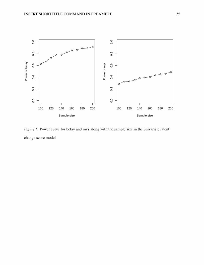
Example 3. Generate a power curve for different sample sizes for a univariate LCSM

Example 2 above showed that a larger sample size is needed in order to get sufficient power

for parameters betay and mys. Although one can try a difference sample size greater than 100, for

convenience, we can generate a power curve with multiple different sample sizes. For example,

Figure 5 shows the power curves for the two parameters betay and mys with sample sizes ranging

from 100 to 200 with an interval 10. From the plot, we can easily see that to get a power 0.8 for

the parameter betay, a sample size about 150 is needed. On the other hand, a sample size larger

than 200 is needed for the parameter mys to have a power 0.8, with the exact number undecided

based on the plot.

The R code for generating the power curve is shown in Code 5. Note that in the plot

function, we refer to a specific parameter directly using its name. In the input, seq(100, 200,

10) generate a sequence of sample sizes and in the output, power for each sample size is

provided. Code 6 shows the output when the sample sizes are 100 and 200 only to save space.

Code 5: R input script for power curve in Example 3.

res <- powerLCS(N = seq(100, 200, 10), T = 5, R = 1000, betay =

0.1, my0 = 20, mys = 1.5, varey = 9, vary0 = 2.5, varys = .05,

vary0ys = 0, alpha = 0.05)

plot(res, 'betay')

plot(res, 'mys')

Code 6: Output for generating power curves in Example 3.

$`N100-T5`


betay 0.10 0.100 0.044 0.044 0.627 100 5

my0 20.00 20.002 0.331 0.319 1.000 100 5

mys 1.50 1.505 1.136 1.119 0.287 100 5

varey 9.00 8.970 0.744 0.732 1.000 100 5


vary0 2.50 2.489 1.218 1.146 0.599 100 5

vary0ys 0.00 -0.009 0.413 0.403 0.059 100 5

varys 0.05 0.054 0.176 0.175 0.050 100 5

....

$`N200-T5`


betay 0.10 0.100 0.031 0.031 0.915 200 5

my0 20.00 20.002 0.225 0.226 1.000 200 5

mys 1.50 1.505 0.790 0.791 0.487 200 5

varey 9.00 8.971 0.532 0.518 1.000 200 5

vary0 2.50 2.480 0.803 0.808 0.904 200 5

vary0ys 0.00 0.005 0.283 0.283 0.049 200 5

varys 0.05 0.051 0.125 0.122 0.054 200 5

Example 4. Generate a power curve for different number of occasions for a univariate

LCSM

For LCSMs, power is not only related to the sample size but also the number of

measurement occasions. With the increase of the number of occasion, one would expect the

increase of power. For example, Figure 6 shows the power curves for the two parameters betay

and mys with the number of occasions ranging from 4 to 10 with an interval 1 and with the fixed

sample size 100. From the plot, we can easily see that the power increases along with the number

of measurement occasions. For example, for the same sample size 100, the power is less than 0.2

with 4 occasions of data but increases to more than 0.8 with 7 occasions of data. The R code for

generating the power curve is shown in Code 7.

Code 7: R input script for power curve with the number of occasions in Example 4.


res <- powerLCS(N = 100, T = 4:10, R = 1000, betay = 0.1, my0 =

20, mys = 1.5, varey = 9, vary0 = 2.5, varys = .05, vary0ys =

0, alpha = 0.05)

Example 5. Power analysis for a bivariate LCSM

Power analysis can be similarly conducted for bivariate LCSMs. As an example, we use the

parameter estimates from a bivariate latent change score model in Zhang et al. (2015) with some

modification as population parameter values (see Table 2).

The script in Code 8 shows the R code for power analysis for the bivariate LCSM with the

sample size 100. From the output in Code 9, we can see that the parameter estimates are not very

accurate. This is because the bivariate LCSM requires a much larger sample size to provide

accurate parameter estimates. In this case, the statistical power obtained might not be accurate

either.

Code 8: R input script for power analysis for bivariate latent change score model in Example 5.

powerBLCS(N=100, T=5, R=1000, betay=0.08, my0=20, mys=1.5, varey

=9, vary0=3, varys=1, vary0ys=0, alpha=0.05, betax=0.2, mx0

=20, mxs=5, varex=9, varx0=3, varxs=1, varx0xs=0, varx0y0=1,

varx0ys=0, vary0xs=0, varxsys=0, gammax=0, gammay=-.1)

Code 9: Output for power analysis in Example 5.


betax 0.20 0.230 0.260 0.187 0.241 100 5

betay 0.08 0.164 0.572 0.435 0.081 100 5

gammax 0.00 -0.033 0.234 0.178 0.112 100 5

gammay -0.10 -0.175 0.641 0.458 0.075 100 5

mx0 20.00 20.004 0.336 0.326 1.000 100 5

mxs 5.00 5.933 7.848 5.615 0.167 100 5


my0 20.00 20.019 0.346 0.326 1.000 100 5

mys 1.50 0.451 6.933 5.321 0.156 100 5

varex 9.00 8.941 0.744 0.732 1.000 100 5

varey 9.00 8.939 0.749 0.720 1.000 100 5

varx0 3.00 3.029 1.243 1.222 0.739 100 5

varx0xs 0.00 -0.210 0.768 0.767 0.030 100 5

varx0y0 1.00 1.052 0.840 0.835 0.226 100 5

varx0ys 0.00 -0.012 0.668 0.601 0.017 100 5

varxs 0.60 2.343 6.805 2.687 0.090 100 5

varxsys 0.00 0.072 3.559 1.740 0.019 100 5

vary0 3.00 2.951 1.423 1.245 0.684 100 5

vary0xs 0.00 0.198 2.263 1.629 0.031 100 5

vary0ys 0.00 -0.371 1.970 1.511 0.106 100 5

varys 0.05 1.415 3.730 2.096 0.024 100 5

Increasing the sample size will lead to more accurate results as shown in Code 10 where the

sample size is 500. In planning the sample size for LCSM models, one should pay attention to the

parameter estimates to make sure they are accurate enough for power calculation. Specifically for

the coupling parameters gammax and gammay, the power, type I error for gammax, is 0.057 and

0.271, respectively.

Code 10: Output for power analysis in Example 5 when the sample size is 500.


betax 0.20 0.2009 0.031 0.031 1.000 500 5

betay 0.08 0.0830 0.070 0.068 0.199 500 5

gammax 0.00 -0.0014 0.030 0.029 0.057 500 5

gammay -0.10 -0.1022 0.072 0.073 0.271 500 5

mx0 20.00 19.9911 0.145 0.145 1.000 500 5


mxs 5.00 5.0308 0.939 0.942 1.000 500 5

my0 20.00 19.9999 0.143 0.146 1.000 500 5

mys 1.50 1.4684 0.889 0.885 0.420 500 5

varex 9.00 8.9836 0.340 0.328 1.000 500 5

varey 9.00 8.9961 0.341 0.328 1.000 500 5

varx0 3.00 3.0052 0.524 0.523 1.000 500 5

varx0xs 0.00 -0.0144 0.222 0.230 0.047 500 5

varx0y0 1.00 1.0064 0.360 0.360 0.808 500 5

varx0ys 0.00 -0.0012 0.199 0.201 0.051 500 5

varxs 1.00 1.0312 0.180 0.189 1.000 500 5

varxsys 0.00 0.0028 0.161 0.163 0.045 500 5

vary0 3.00 2.9777 0.519 0.547 1.000 500 5

vary0xs 0.00 0.0072 0.286 0.294 0.035 500 5

vary0ys 0.00 -0.0135 0.252 0.257 0.043 500 5

varys 1.00 1.0246 0.260 0.253 0.999 500 5

Discussion and Future Directions

To complement the research on LCSMs, in this chapter, we discuss how to plan the sample

size and number of measurement occasions for both univariate and bivariate LCSMs. Specifically,

we illustrate how to calculate power for each individual model parameter of interest. Since the

analytical solution to power is untraceable, we used a Monte Carlo based method. We also

provided an R package RAMpath and an online interface to carry out the power analysis

procedure.

In calculating power, we need the information on the population parameter values. Each

value can be viewed as the unstandardized effect size for the parameter of interest. We did not

define the standardized effect size such as Cohen’s d (Cohen, 1988) for several reasons. First,

given the complexity of LCSMs, it is difficult to define a standardized effect size. Second, in


general, it is easier to specify the unstandardized effect size because when conducting a literature

review, one can simply adopt the parameter estimates directly from published results. Third, if a

researcher is interested in standardized measures, he/she can use the standardized coefficients as

the population parameter values in conducting power analysis. But note even in such condition,

power from different studies might not be comparable.

The current study can be improved in many ways in the future. First, in this chapter, we

have focused on the power analysis of a single model parameter as this is the most common

situation. If a researcher wants to test multiple parameters simultaneously, a procedure based on

the likelihood ratio test can be developed as for the growth curve analysis in Zhang & Wang

(2009).

Second, in the current study, we have focused on the basic univariate and bivariate LCSMs.

Since their invention, the basic univariate and bivariate LCSMs have been extended in many ways.

For example, Hamagami & McArdle (2007b) expanded the traditional specifications of univariate

and bivariate LCSMs to the parallel process change score model and the second-order LCSMs.

Grimm et al. (2012) extended latent difference scores to allow for testing hypotheses where recent

changes, as opposed to recent levels, are a primary predictor of subsequent changes. The Monte

Carlo procedure used in this study can be flexibly extended to the more advanced models.

Third, the current study has assumed that the collected data will be complete. However, in

practice, missing data are almost not avoidable in longitudinal studies. For example, Puma et al.

(2009) found that student achievement outcomes are often missing for 10-20% in studies funded

by the National Center for Education Evaluation and Regional Assistance. Missing data reduce

power and without careful consideration, a well-planned study can become under-powered.

Taking into consideration of missing data in power calculation requires the specification of

missing data generating mechanism that can be used in the data generation step in our Monte

Carlo method.

Third, in our Monte Carlo method, we have assumed that our data are normally distributed.

However, practical data often deviate from a normal distribution. For example, Micceri (1989)


evaluated 440 large-sample achievement and psychometric measures distributions and found that

all of them were nonnormal. More recently, Blanca et al. (2013) evaluated nonnormality using the

skewness and kurtosis of 693 small samples and found that 94.5 % of them violated the normality

assumption. In addition, Cain et al. (2016) reviewed 254 multivariate distributions of data used in

Psychological Science and the American Education Research Journal and found that 68 %

multivariate distributions deviated from normal distributions. Therefore, in the future, the

influence of non-normal data should be considered when estimating power.

Finally, the Monte Carlo based method can be very computationally intensive because of

the involvement of the Monte Carlo simulation. For example, it took about 10 minutes on a

modern desktop to complete the power analysis in Example 4. At the same time, the Monte Carlo

method can be easily parallelized to take advantage of modern hardware such as multi-core

processors (e.g., Zhang, 2014). In the future, the R package RAMpath can be improved with the

capacity of parallelization.


References

Blanca, M. J., Arnau, J., López-Montiel, D., Bono, R., & Bendayan, R. (2013). Skewness and

kurtosis in real data samples. Methodology.

Boker, S. M., McArdle, J. J., & Neale, M. C. (2002). An algorithm for the hierarchical

organization of path diagrams and calculation of components of covariance between variables.

Structural Equation Modeling, 9(2), 174–194.

Boker, S. M., Neale, M., Maes, H., Wilde, M., Spiegel, M., Brick, T., . . . others (2011). Openmx:

an open source extended structural equation modeling framework. Psychometrika, 76(2),

306–317.

Browne, M. W. (1993). Structured latent curve models. In C. M. Cuadras & C. R. Rao (Eds.),

Multivariate analysis: Future directions 2 (pp. 171–198). Amsterdam: North-Holland.

Cain, M. K., Zhang, Z., & Yuan, K.-H. (2016). Univariate and multivariate skewness and kurtosis

for measuring nonnormality: Prevalence, influence and estimation. Behavior Research

Methods, 1–20.

Cohen, J. (1988). Statistical power analysis for the behavioral sciences (2nd ed.). Hillsdale, NJ:

Lawrence Ehrlbaum Associates.

Enders, C. K. (2011). Missing not at random models for latent growth curve analyses.

Psychological methods, 16(1), 1–16.

Fox, J. (2006). Structural equation modeling with the sem package in r. Structural Equation

Modeling, 13, 465–486.

Gerstorf, D., Lövdén, M., Röcke, C., Smith, J., & Lindenberger, U. (2007). Well-being affects

changes in perceptual speed in advanced old age: longitudinal evidence for a dynamic link.

Developmental psychology, 43(3), 705.


Ghisletta, P., & Lindenberger, U. (2005). Exploring the structural dynamics of the link between

sensory and cognitive functioning in old age: Longitudinal evidence from the berlin aging

study. Intelligence, 33, 555–587.

Ghisletta, P., & McArdle, J. J. (2012). Latent curve models and latent change score models

estimated in r. Structural equation modeling: a multidisciplinary journal, 19(4), 651–682.

Grimm, K. J., An, Y., McArdle, J. J., Zonderman, A. B., & Resnick, S. M. (2012). Recent

changes leading to subsequent changes: Extensions of multivariate latent difference score

models. Structural equation modeling: a multidisciplinary journal, 19(2), 268–292.

Grimm, K. J., Ram, N., & Estabrook, R. (2016). Growth modeling: Structural equation and

multilevel modeling approaches. Guilford Publications.

Grimm, K. J., Ram, N., & Hamagami, F. (2011). Nonlinear growth curves in developmental

research. Child development, 82(5), 1357–1371.

Hamagami, F., & McArdle, J. J. (2007a). Dynamic extensions of latent difference score models.

In S. M. Boker & M. J. Wenger (Eds.), Data analytic techniques for dynamical systems (pp.

47–86). Mahwah, NJ: Erlbaum.

Hamagami, F., & McArdle, J. J. (2007b). Dynamic extensions of latent difference score models.

In S. M. Boker & Wenger (Eds.), Data analytic techniques for dynamical systems (pp. 47–85).

Mahwah, NJ: Lawrence Erlbaum Associates, Inc.

Hamagami, F., Zhang, Z., & McArdle, J. J. (2010). Bayesian discrete dynamic system by latent

difference score structural equations models for multivariate repeated measures data. In

S.-M. Chow, E. Ferrer, & F. Hsieh (Eds.), Statistical methods for modeling human dynamics:

An interdisciplinary dialogue (pp. 319–348). New York, NY: RoutledgeTaylor & Francis

Group.


Hedges, L. V., & Rhoads, C. (2010). Statistical power analysis in education research. ncser

2010-3006. National Center for Special Education Research.

King, L. A., King, D. W., McArdle, J. J., Saxe, G. N., Doron-LaMarca, S., & Orazem, R. J.

(2006). Latent difference score approach to longitudinal trauma research. Journal of traumatic

stress, 19(6), 771–785.

Lu, Z. L., Zhang, Z., & Cohen, A. (2013). Bayesian methods and model selection for latent

growth curve models with missing data. In New developments in quantitative psychology (pp.

275–304). Springer.

McArdle, J. J. (1986). Latent variable growth within behavior genetic models. Behavior

Genetics, 16, 163-200.

McArdle, J. J. (1998). Modeling longitudinal data by latent growth curve methods. In

G. Marcoulides (Ed.), Modern methods for business research (pp. 359–406). Mahwah, NJ:

Lawrence Erlbaum Associates.

McArdle, J. J. (2000). A latent difference score approach to longitudinal dynamic structural

analyses. In R. Cudeck, S. du Toit, & D. Sôrbom (Eds.), Structural equation modeling: Present

and future (pp. 342–380). Lincolnwood, IL: Scientific Software International.

McArdle, J. J. (2009). Latent variable modeling of differences and changes with longitudinal

data. Annual review of psychology, 60, 577–605.

McArdle, J. J., & Anderson, E. (1990). Latent variable growth models for research on aging. In

J. E. Birren & K. W. Schaie (Eds.), Handbook of the psychology aging (p. 21-44). New York:

Academic Press.

McArdle, J. J., & Bell, R. Q. (1998). Recent trends in modeling longitudinal data by latent

growth curve methods. In T. D. Little, K. U. Schnabel, & J. Baumert (Eds.), Modeling


longitudinal and multiple-group data: Practical issues, applied approaches, and scientific

examples (p. 69-107). Mahwah, NJ: Erlbaum.

McArdle, J. J., & Boker, S. M. (1990). Rampath. Hillsdale, NJ: Lawrence Erlbaum.

McArdle, J. J., & Epstein, D. (1987). Latent growth curves within developmental structural

equation models. Child Psychology, 58, 110-133.

McArdle, J. J., & Hamagami, F. (1992). Modeling incomplete longitudinal and cross–sectional

data using latent growth structural models. Experimental Aging Research, 18(3), 145–166.

McArdle, J. J., & Hamagami, F. (2001). Latent difference score structural models for linear

dynamic analyses with incomplete longitudinal data. In L. M. Collins & A. G. Sayer (Eds.),

New methods for the analysis of change (pp. 139–175). Washington, DC: American

Psychological Association.

McArdle, J. J., & Nesselroade, J. R. (1994). Using multivariate data to structure developmental

change. In S. H. Cohen & H. W. Reese (Eds.), Life-span developmental psychology:

Methodological contributions (pp. 223–267). Hillsdale, NJ: Lawrence Erlbaum Associates.

McArdle, J. J., & Nesselroade, J. R. (2014). Longitudinal data analysis using structural equation

models. American Psychological Association.

Micceri, T. (1989). The unicorn, the normal curve, and other improbable creatures.

Psychological Bulletin, 105(1), 156–166.

Muthén, L. K., & Muthén, B. O. (2002). How to use a monte carlo study to decide on sample size

and determine power. Structural Equation Modeling, 9(4), 599–620.

Myors, B., & Wolach, A. (2014). Statistical power analysis: A simple and general model for

traditional and modern hypothesis tests. Routledge.

Neale, M. C., & McArdle, J. J. (2000). Structured latent growth curves for twin data. Twin

Research, 3, 165–177.


Puma, M. J., Olsen, R. B., Bell, S. H., & Price, C. (2009). What to do when data are missing in

group randomized controlled trials. ncee 2009-0049. National Center for Education Evaluation

and Regional Assistance.

Raz, N., Lindenberger, U., Ghisletta, P., Rodrigue, K. M., Kennedy, K. M., & Acker, J. D. (2008).

Neuroanatomical correlates of fluid intelligence in healthy adults and persons with vascular

risk factors. Cerebral Cortex, 18(3), 718–726.

Rosseel, Y. (2012). lavaan: An R package for structural equation modeling. Journal of Statistical

Software, 48, 1–36.

Shadish, W. R., Cook, T. D., & Campbell, D. T. (2002). Experimental and quasi-experimental

designs for generalized causal inference. Wadsworth Cengage learning.

Thoemmes, F., MacKinnon, D. P., & Reiser, M. R. (2010). Power analysis for complex

mediational designs using monte carlo methods. Structural Equation Modeling, 17, 510–534.

Wang, L., & McArdle, J. J. (2008). A simulation study comparison of Bayesian estimation with

conventional methods for estimating unknown change points. Structural Equation Modeling,

15, 52–74.

Yuan, K.-H., & Zhang, Z. (2012). Robust structural equation modeling with missing data and

auxiliary variables. Psychometrika, 77, 803–826.

Zhang, Z. (2013). Bayesian growth curve models with the generalized error distribution. Journal

of Applied Statistics, 40, 1779–1795.

Zhang, Z. (2014). Monte carlo based statistical power analysis for mediation models: Methods

and software. Behavior research methods, 46(4), 1184–1198.

Zhang, Z., Hamagami, F., Grimm, K. J., & McArdle, J. J. (2015). Using r package rampath for

tracing sem path diagrams and conducting complex longitudinal data analysis. Structural

Equation Modeling: A Multidisciplinary Journal, 22(1), 132–147.


Zhang, Z., Lai, K., Lu, Z., & Tong, X. (2013). Bayesian inference and application of robust

growth curve models using student’s t distribution. Structural equation modeling, 20, 47–78.

Zhang, Z., & Wang, L. (2009). Statistical power analysis for growth curve models using sas.

Behavior Research Methods, 41, 1083–1094.


Table 1

Population parameter values used in Examples 1-4

Example 1 Example 2

betay 0 0.1

my0 0 20

mys 0 1.5

varey 1 9

vary0 1 2.5

varys 1 0.05

vary0ys 0 0


Table 2

Population parameter values used in Example 5

Parameter value Parameter value

betay 0.08 betax 0.2

gammax 0 gammay −0.1

my0 20 mx0 20

Mys 1.5 mxs 5

varey 9 varex 9

vary0 3 varx0 3

varys 0.05 varxs 0.6

vary0ys 0 varx0xs 0

varx0y0 1 @x M @x M

vayx0ys 0 @x M @x M

vary0xs 0 @x M @x M

varxsys 0 @x M @x M


1 2 3 4 5

510

15

Time

y[t]

beta=0beta=0.1beta=0.5beta=1

Figure 1. The trajectory plot of latent scores y[t] from time 1 to time 5 with different βy values


y1

y0

Y1

1

1

e1

1

y2

dy2

Y2

1

1

e2

1

y3

dy3

Y3

1

1

e3

1

yT

dyT

YT

1

1

eT

1

ys

...

...

1 1 1 1

1 1 11

1

betay betay betay betay

my0mys

vary0

varysvary0ys

varey varey varey varey

Figure 2. Path diagram for a univariate latent change score models


y1

y0

Y1

1

y2

dy2

Y2

1

1

y3

dy3

Y3

1

1

yT

dyT

YT

1

1

ys

...

...

1 1 1 1

1

betay betay betay betay

mys

vary0

varys

vary0ys

varey varey varey varey

x1

x0

X1

1

x2

dx2

X2

1

1

x3

dx3

X3

1

1

xT

dxT

XT

1

1

xs

...

...

1 1 1 1

betax betax betax betax

varx0

varxs

varx0xs

varex varex varex varex

my0

mxsmx0

varxsys

gammax gammax gammax gammax

gammay gammay gammay gammay

1

1

1

1

varx0y0

varx0ys

vary0xs

Figure 3. The path diagram for a bivariate latent change score model.


Figure 4. The online interface for power analysis for univariate latent change score models.


100 120 140 160 180 200

0.0

0.2

0.4

0.6

0.8

1.0

Sample size

Pow

er o

f bet

ay ●

●

●

● ●

●● ●

● ●●

100 120 140 160 180 2000.

00.

20.

40.

60.

81.

0Sample size

Pow

er o

f mys

●● ●

●● ● ●

●● ●

●

Figure 5. Power curve for betay and mys along with the sample size in the univariate latent

change score model


4 5 6 7 8 9 10

0.0

0.2

0.4

0.6

0.8

1.0

Number of Occasions

Pow

er

●

●

● ● ● ● ●

4 5 6 7 8 9 100.

00.

20.

40.

60.

81.

0Number of Occasions

Pow

er

●

●

●

●

● ● ●

Figure 6. Power curve for betay and mys along with the number of measurement occasions in the

univariate latent change score model

sample size and measurement occasion planning for latent

Documents