salt river project 700 mhz draft report - utc

Salt River 700 MHz Field Test Report

January 20, 2015

Contents Overview ....................................................................................................................................................... 3

Throughput Capability .................................................................................................................................. 4

Required Throughput .................................................................................................................................... 5

Coverage ....................................................................................................................................................... 6

Details of Coverage Test and Results ........................................................................................................... 7

Interference ................................................................................................................................................... 9

Choice of Modulation ................................................................................................................................. 11

Constant Envelope Modulation ................................................................................................................... 13

FSK Signal and Modulator ......................................................................................................................... 14

Power Spectral Density ............................................................................................................................... 15

Performance in Interference ........................................................................................................................ 20

Overall Spectral Efficiency ......................................................................................................................... 22

Network and Control Layer ........................................................................................................................ 23

Summary ..................................................................................................................................................... 24

Figure 1 . Required Number of Spectral Slices per Reuse Pattern. ............................................................. 4 Figure 2. Relative Throughput per Reuse Pattern. ....................................................................................... 5 Figure 3. Representative Path Loss per Hata. .............................................................................................. 6 Figure 4. Test Locations and Paths to PBF .................................................................................................. 7 Figure 5 Elevation Profile for Path 12. ........................................................................................................ 8 Figure 6. Elevation Profile for Path 13. ....................................................................................................... 8 Figure 7. Measured Path Loss Compared to Hata’s View of Okumura. ...................................................... 8 Figure 8. Statistical Parameters of Measured Propagation Loss. ................................................................. 9 Figure 9. Error Rate vs Distance. ................................................................................................................. 9 Figure 10. Number of Subscribers connected to Verizon Site. .................................................................. 10 Figure 11. Verizon Receiver Noise Level .................................................................................................. 11 Figure 12. Bit Error Probability of M-FSK. ............................................................................................... 14 Figure 13. Power-density spectrum of BFSK signal (for h = 0.5, 0.6, 0.7). ............................................... 15 Figure 14. Power-density spectrum of BFSK signal (for h = 0.8, 0.9, 0.95). ............................................. 16 Figure 15 Power-density spectrum of 4-FSK signal (for h = 0.2, 0.35, and 0.4). ....................................... 16 Figure 16. Power-density spectrum of 4-FSK signal (for h = 0.5, 0.6, and 0.7). ....................................... 17 Figure 17. Power-density spectrum of 8-FSK signal (for h = 0.125, 0.2, and 0.3). .................................... 17 Figure 18. Power-density spectrum of 8-FSK signal (for h = 0.4, 0.5, and 0.6). ........................................ 18 Figure 19. Power spectra of M-ary FSK signals for M = 2, 4, and 8 (h = 0.5). .......................................... 19 Figure 20. Performance in Interference and Noise of 2-FSK. ................................................................... 20 Figure 21. Performance in Interference and Noise of 4-FSK. ................................................................... 21 Figure 22. Performance in Interference and Noise of 8-FSK. ................................................................... 21 Figure 23. Performance in Interference Only of 2-, 4-, and 8-FSK ........................................................... 22 Figure 24. A Mesh Network. ...................................................................................................................... 23

Page 2 of 25 © 2015 ConVergence and Memorylink 1/20/2015

Overview ConVergence Technologies, Inc. was tasked with designing and building a proof-of-concept system focused on the application of the 700 MHz Upper A-block spectrum (two one-Megahertz slots) to the “Smart Grid” system that the Salt River Project foresees. We completed that task, successfully, producing an experimental system that closely adhered to the desired specifications, and conducted a coverage test in SRP’s territory to validate the concepts. That test also included an evaluation of the potential for interference to and from the Verizon LTE system on adjacent spectrum, with the appropriate extension to the future Public Safety system that will also be nearby.

Coverage in this spectrum is much as predicted. Our field test results agree well with predictions made with the common tools, such as Okumura. Of course, the Phoenix area is somewhat unique in that it is largely composed of what Okumura would call suburban scattered among a number of small mountains (or steep hills).

Our bottom-line conclusion is that the spectrum in question is definitely suitable for SRP’s use, as long as the appropriate technical features are implemented. These features, in no particular order, are as follows:

1. Time-division duplex operation, with automatic selection between the two frequencies. 2. Careful design of the modulation method, to allow for maximum performance in

interference; this is critical to the very high frequency reuse that this system is capable of. 3. The use of directional antennas on both the Access Point and Client units; this is also

essential to maintaining the best frequency reuse. We foresee that the implementation of electrically steerable antennas on the Client units will not add significantly to the cost.

4. The implementation of a self-directed mesh network, to minimize the number of Access Points required for complete area coverage and to maximize the overall data throughput capability.

5. Variable data rate, to allow larger cells as the system is first turned up. Ideally, the faster data rates will exhibit the same resistance to interference as the slower, unlike Wi-Fi and cellular system currently in use.

6. Intelligence in all units to avoid causing interference. There is a small area around each of Verizon’s cell sites (less than 500 feet in diameter) within which an SRP station operating in the higher of the two band segments can cause some interference to the cellular network. It should be noted that our investigation, with Verizon’s help, shows conclusively that the problem lies in the selectivity limitations of the receivers Verizon employs; no amount of further reduction in the out-of-band emissions of the SRP equipment will reduce the problem.

7. The system chosen should exhibit the proper economic characteristics; the right “experience curve” as system volumes increase:

a. It should not rely on “borrowing” technology from another system whose widely differing aims will cause divergence in the years ahead;

b. It should be practical at the initial volumes that SRP expects in the first couple of years of deployment;


c. It should scale smoothly to the much higher volumes to be hoped for as more utilities adopt the concepts;

d. And it must be realized that the volumes for this system, although quite large, and of a significantly different magnitude than those of Cellular Telephone or Wi-Fi, for example.

All of the above areas are expanded upon in the sections below.

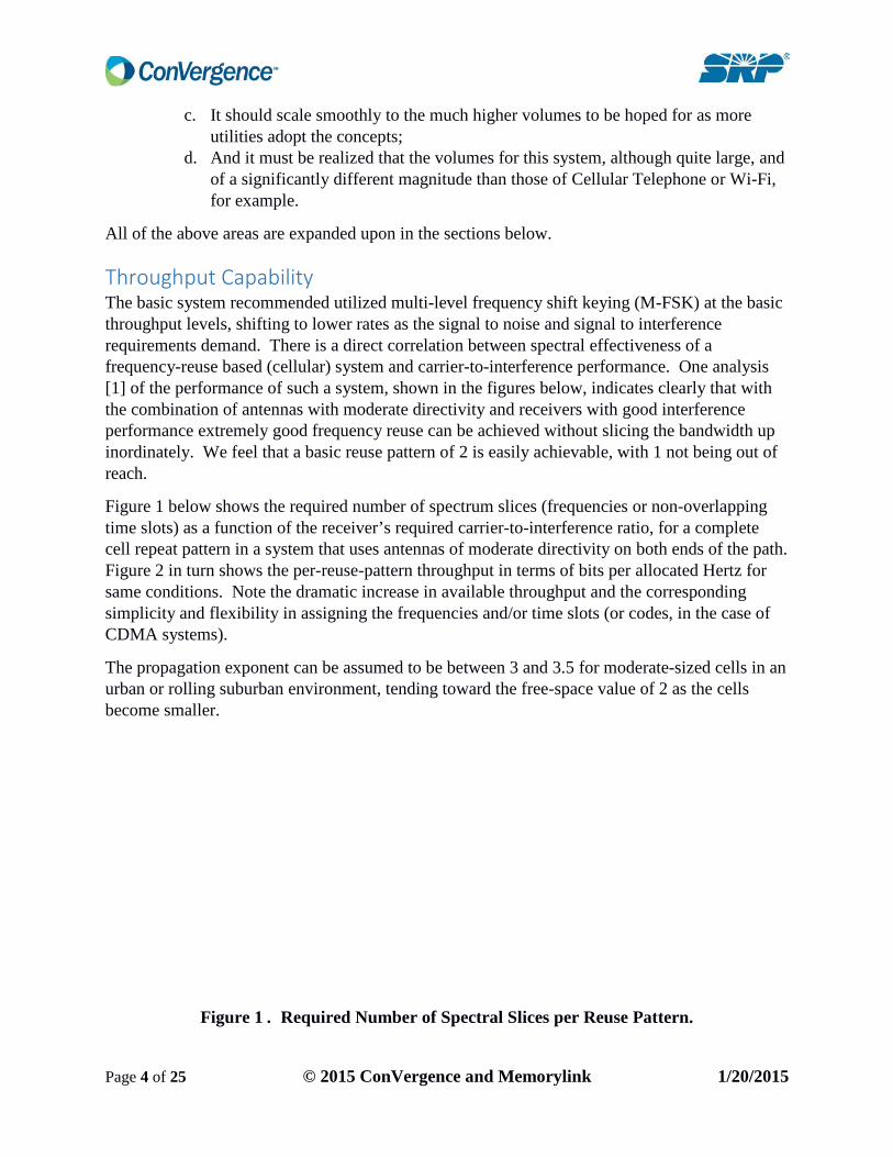
Throughput Capability The basic system recommended utilized multi-level frequency shift keying (M-FSK) at the basic throughput levels, shifting to lower rates as the signal to noise and signal to interference requirements demand. There is a direct correlation between spectral effectiveness of a frequency-reuse based (cellular) system and carrier-to-interference performance. One analysis [1] of the performance of such a system, shown in the figures below, indicates clearly that with the combination of antennas with moderate directivity and receivers with good interference performance extremely good frequency reuse can be achieved without slicing the bandwidth up inordinately. We feel that a basic reuse pattern of 2 is easily achievable, with 1 not being out of reach.

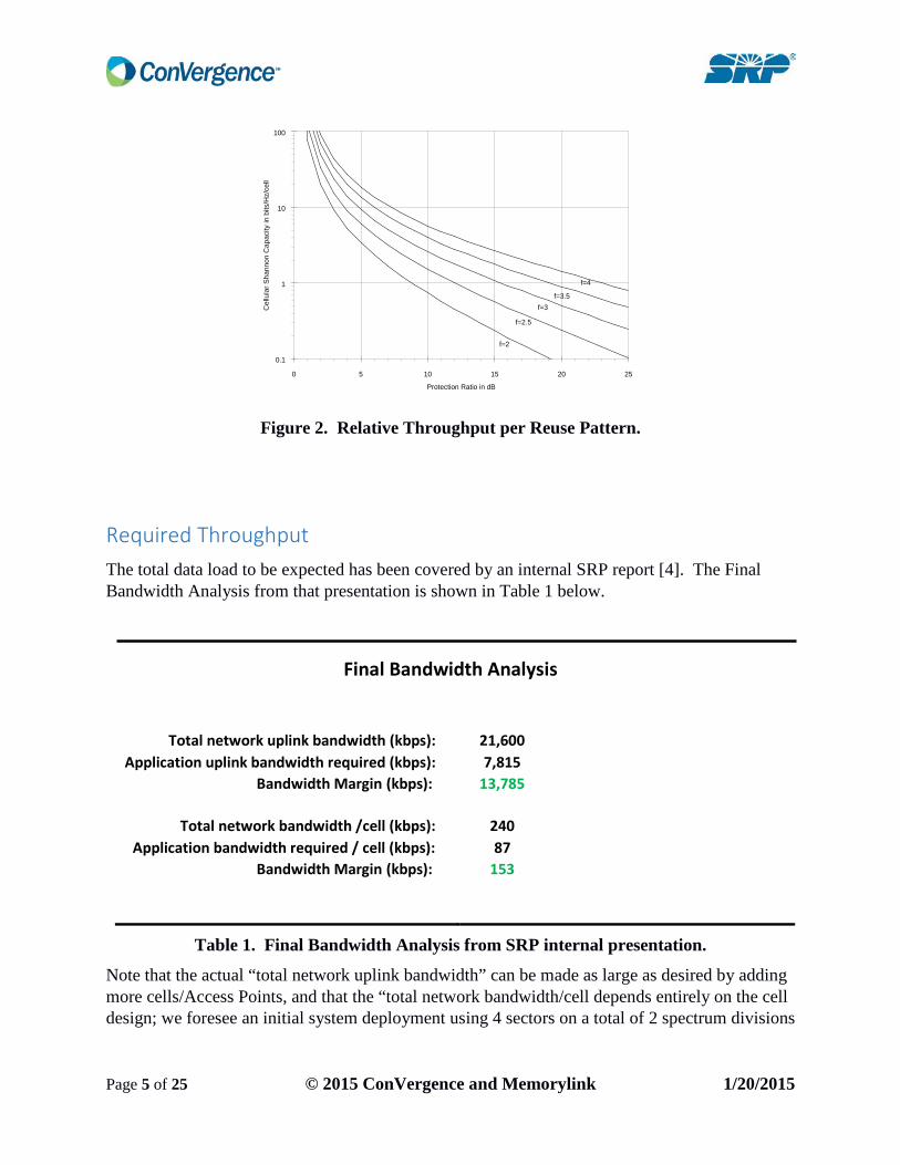
Figure 1 below shows the required number of spectrum slices (frequencies or non-overlapping time slots) as a function of the receiver’s required carrier-to-interference ratio, for a complete cell repeat pattern in a system that uses antennas of moderate directivity on both ends of the path. Figure 2 in turn shows the per-reuse-pattern throughput in terms of bits per allocated Hertz for same conditions. Note the dramatic increase in available throughput and the corresponding simplicity and flexibility in assigning the frequencies and/or time slots (or codes, in the case of CDMA systems).

The propagation exponent can be assumed to be between 3 and 3.5 for moderate-sized cells in an urban or rolling suburban environment, tending toward the free-space value of 2 as the cells become smaller.

Figure 1 . Required Number of Spectral Slices per Reuse Pattern.


Protection Ratio in dB

Cel

lula

r Sha

nnon

Cap

acity

in b

its/H

z/ce

ll

0.1

1

10

100

0 5 10 15 20 25

f=4

f=3.5f=3

f=2.5

f=2

Figure 2. Relative Throughput per Reuse Pattern.

Required Throughput The total data load to be expected has been covered by an internal SRP report [4]. The Final Bandwidth Analysis from that presentation is shown in Table 1 below.

Final Bandwidth Analysis

Total network uplink bandwidth (kbps): 21,600 Application uplink bandwidth required (kbps): 7,815

Bandwidth Margin (kbps): 13,785

Total network bandwidth /cell (kbps): 240 Application bandwidth required / cell (kbps): 87

Bandwidth Margin (kbps): 153

Table 1. Final Bandwidth Analysis from SRP internal presentation.

Note that the actual “total network uplink bandwidth” can be made as large as desired by adding more cells/Access Points, and that the “total network bandwidth/cell depends entirely on the cell design; we foresee an initial system deployment using 4 sectors on a total of 2 spectrum divisions


(time slots and/or frequencies, in a 1-2-1-2 pattern, one spectrum division per sector), allowing for a starting point of at least 2.8 Mbps per cell site.

Coverage The above discussion pretty well handles the aspect of minimum cell size. Maximum cell size is a matter of propagation – the range that can be expected for a given frequency, transmitter power, and receiver sensitivity.

There have been many models of propagation in non-line-of-sight conditions developed over the years. Perhaps the most popular are derived from the work of Yoshihisa Okumura and others, who made a very large study of land-mobile propagation in and around Tokyo in the early 1960s. Hata [2] did a good job of reducing the mass of data Okumura et al collected into a set of formulas that could easily be applied to computer solutions, given some reasonable generalizations about the characteristics of the terrain involved.

Figure 3 shows some representative numbers for a base antenna system consisting of a representative 9 dB gain antenna with a 90⁰ beamwidth, at a height of 45 meters.

Figure 3. Representative Path Loss per Hata.

Our coverage measurements showed reasonable agreement with these numbers, allowing for the shadowing effects of mountains and large buildings. 750 MHz is quite a reasonable frequency in terms of propagation.

0.00

20.00

40.00

60.00

80.00

100.00

120.00

140.00

160.00

0.01 0.1 1 10 100

Path

Los

s, d

B

Distance in Miles

Path Loss per Hata's view of Okumura

Omni CM on car Omni CM at 45 feet Yagi CM at 45 feet


Details of Coverage Test and Results The coverage test was conducted with the following conditions:

• The ConVergence-supplied transmitter was set up at the access point (most of the data was taken from PBF).

• Transmitter power was set to 2 watts. • The gain of the transmitting antenna was 9 dB. • A data test stream was established consisting of a 1 KHz sine wave digitized at 200 Kbps. • No error correction was implemented. • An omnidirectional antenna of 0 dB gain was mounted on the roof of the test vehicle. • The test data stream was received by a ConVergence-supplied receiver connected to the

vehicle antenna. • The error rate was estimated by ear; previous tests have shown this to be accurate to

within 2 to 3 dB of signal strength. • The actual signal strength was simultaneously measured with an appropriate spectrum

analyzer, using its hand-held antenna (log periodic, 5 dB of gain). • The location of each test point was recorded using GPS, and the above readings included

in the record.

The data described above is reproduced in Appendix 1. The selected locations and the corresponding paths to PBF, as plotted in Google Earth, are shown in Figure 4 below. The KML file used by Google Earth to represent this data is available upon request.

Figure 4. Test Locations and Paths to PBF


To provide a picture of the terrain involved, Figure 5 and Figure 6 show the terrain profile for two representative paths.

Figure 5 Elevation Profile for Path 12.

Figure 6. Elevation Profile for Path 13.

Several different analyses were undertaken to conclusively determine if the propagation characteristics of the spectrum are suitable for the applications. First, we compared the path loss as measured to that predicted by Hata’s view of Okumura. The results are shown in Figure 7 below. The orange dots and line are the predictions.

Figure 7. Measured Path Loss Compared to Hata’s View of Okumura.

80

90

100

110

120

130

140

150

0.1 1 10

Path

Los

s, d

B

Distance, Miles


The statistical parameters of the fit, expressed as the difference between the two numbers for any one distance, are as follows:

• Standard Deviation : 6.34 dB • Mean: 1.24 dB • Median: 1.09 dB

Figure 8. Statistical Parameters of Measured Propagation Loss.

The typical assumption for an urban area, or a suburban area with rolling terrain, is a standard deviation of 6 dB. By these measures, our data fits the Okumura model exceedingly well.

The observed error rate vs distance performance is shown in Figure 9 below. The dotted line is a logarithmic trendline which closely follows the Hata/Okumura path loss transformed by the signal-to-noise vs error rate predominance of our M-FSK modulation.

Figure 9. Error Rate vs Distance.

Interference We looked at interference both from and to the Verizon LTE network that operates in the adjacent spectrum. For the case of interference to our system, we conducted some of our coverage tests in areas immediately adjacent to a heavily-used Verizon transmitter, with the

0.01%

0.10%

1.00%

10.00%

100.00%

0.1 1 10

Erro

r Rat

e

Distance, Miles


client receiver in the portion of our spectrum closest to the frequency of the Verizon transmitters (the lower segment). No effect was found.

For the case of interference to the LTE system, we conducted a carefully crafted experiment in cooperation with the Verizon engineering staff. One of our access points was set up in a substation yard that also hosts a Verizon cell site. We set up a one-sector cell, using a directional antenna on a 50-foot pole situated 160 feet from the Verizon antenna structure; our antenna was pointed at right angles to a line from our site to Verizon’s; at this angle our antenna has a gain of about zero dB. We radiated 2 watts in the prime direction of our antenna; this corresponds to ¼ watt, or +24 dBm, in the direction towards the LTE antenna.

At that level, the Verizon engineers reported that the noise level into their receiver was increased by 6 dB.

Verizon provided us with a chart that shows the number of cellular subscribers connected to the site adjacent to our AP. See Figure 10 below. The blue arrows show the generally smooth increase in the number of connected users as the day progresses toward the rush hour. The green arrows show the significant decrease in during the periods of our testing.

Figure 10. Number of Subscribers connected to Verizon Site.

Being uncertain as to whether the degradation was due to out-of-band emission from our transmitter, or simply the limited skirt selectivity of their receiver, we performed another test. We turned off the modulation on our signal, radiating a single carrier frequency with no sidelobes at all.

The results of this test are shown in Figure 11 below. Indeed, the increase in their receiver’s noise floor was the same as in the case where our transmitter was modulated. Therefore, we conclude that the effect is due to the limits of their receiver’s selectivity, not our transmitter’s out-of-band radiation.


Figure 11. Verizon Receiver Noise Level

None the less, this is a significant problem for Verizon, and we might be considered remiss in not addressing it. A simple free-space calculation shows that the 15 dB of further attenuation required to protect their receiver requires a separation of about 1000 feet for one of our system APs aimed directly at their cell site. This means that this problem is a concern for less than 3% of the system area, assuming a one-mile cell radius for our system, and that every cell has a Verizon site near our AP location.

The solution is obvious – merely use only the lower of our frequencies for those problem sites. Indeed, it will be very simple to design the AP radio in such a way that it can listen for nearby LTE transmitters, and then appropriately avoid the associated LTE receivers. Client devices within the “protected” region would not be a problem due to their low duty cycle; the nature of the LTE system corrects for such occasional bursts of interference.

One would hope that the problem could be limited by appropriate redesign of the receivers in the Verizon system, although the problem would probably require more than simply adding a filter in front of the receiver. Of course, interference from sources outside the spectrum licensed to the user are the responsibility of the owners of the receiver, not the “interfering” transmitter. It is with these factors in mind that the FCC decided to make these interstitial segments available for use.

Choice of Modulation A modulation format is the means by which information is encoded unto a signal. Information, or data, can be carried in the amplitude, frequency, or phase of a signal. Modern communication systems use digital modulation techniques. Advancement in very large-scale integration (VLSI) and digital signal processing (DSP) technology have made digital modulation and coherent detection very cost effective. Digital transmissions also are convenient for the implementation of digital error-control codes signal conditioning and processing techniques such as source coding, encryption, and equalization to improve the performance of the overall communication link.


Many digital modulation techniques are used in modern wireless communication systems, and many more are sure to be introduced. Some of these techniques have subtle differences: for example, Frequency Shift Keying (FSK) may be either coherently or noncoherently detected; and may have two, four, eight or more possible levels per symbol.

Several factors influence the choice of a digital modulation scheme. A desirable modulation scheme provides low bit error rates at low received signal-to-noise ratios, performs well in multipath and fading conditions, is very resistant to interference, occupies a minimum bandwidth, and is easy and cost effective to implement. Unfortunately, existing modulation schemes do not simultaneously satisfy all of these requirements; some modulation schemes are better in terms of bit error rate performance, while others are better in terms of bandwidth efficiency

The performance of a modulation scheme can be expressed in terms of its power efficiency; its bandwidth efficiency; and its ability to reject interference, which is crucial to frequency reuse. Power efficiency describes the ability of a modulation technique to preserve the fidelity of the digital message at low power levels. The power efficiency (sometimes called energy efficiency) of a digital modulation scheme is a measure of how favorable the tradeoff between fidelity and signal power is made, and is often expressed as the ratio of the signal energy per bit to noise power spectral density (Eb/No) required at the input of the receiver for a certain probability of error.

Bandwidth efficiency describes the ability of a modulation scheme to accommodate data within a limited bandwidth. In general, increasing the data rate implies decreasing the pulse width of a digital symbol, which increases the bandwidth of the signal. Thus, there is an unavoidable relationship between data rate and bandwidth occupancy. However, some modulation schemes perform better than others in making this tradeoff. Bandwidth efficiency reflects how efficiently the allocated bandwidth is utilized and is defined as the ratio of the throughput data rate per Hertz in a given bandwidth. If R is the data rate in bits per second, and B is the bandwidth occupied by the modulated radio frequency signal, then bandwidth efficiency in one cell ηB is expressed as

ηB = 𝑅𝑅𝐵𝐵 bps/Hz

Ignoring reuse, the system capacity of a digital communication system is directly related to the bandwidth efficiency of the modulation scheme, since a modulation with a greater value of ηB

will transmit more data in a given spectrum allocation.

There is a fundamental upper bound on achievable bandwidth efficiency. Shannon’s channel coding theorem states that for an arbitrary small probability or error, the maximum possible bandwidth efficiency is limited by the noise in the channel, and is given by channel capacity formula. The Shannon’s bound for additive white Gaussian noise (AWGN) non-fading channel is given by:


𝜂𝜂𝐵𝐵𝐵𝐵𝐵𝐵𝐵𝐵 = 𝐶𝐶 𝐵𝐵

= 2(1 + 𝑆𝑆𝑁𝑁

)

where C is the channel capacity in bits per second, B is the radio frequency (RF) bandwidth, and S/N is the signal-to-noise ratio.

Reuse, however, is a crucial system concept. The reuse capability of a given system is directly related to its ability to reject interference; that is, the ratio of signal power to interfering power (C/I) required.

In the design of a digital communication system there is usually a tradeoff among bandwidth efficiency, power efficiency, and reuse. For example, adding error control coding to a message increases the bandwidth occupancy (and this, in turn, reduces the bandwidth efficiency), but at the same time reduces the required power for a particular bit error rate, and hence trades bandwidth efficiency for power efficiency. On the other hand, higher level modulation schemes (M-ary keying), except M-ary FSK, decrease bandwidth occupancy but increase the required received power, and hence trades power efficiency for bandwidth efficiency.

While power and bandwidth considerations are very important, other factors also affect the choice of a digital modulation scheme. For example, for all communication systems which serve a large user community, the cost and complexity of the end-point devices must be minimized, and a modulation which is simple to detect is most attractive. The performance of a modulation scheme under various types of channel impairments such as Rayleigh and Ricean fading and multipath time dispersion, given a particular demodulator implementation, is another key factor in selecting a modulation. In wireless systems where interference is a major issue, the performance of a modulation scheme in an interference environment is extremely important. Sensitivity to detection of time jitter, caused by time-varying channels, is also an important consideration in choosing a particular modulation scheme.

Constant Envelope Modulation Many practical radio communication systems use nonlinear modulation methods, where the amplitude of the carrier is constant, regardless of the variation in the modulating signal. The constant envelope family of modulations has the advantage of satisfying a number of conditions, some of which are:

• Power efficient class C amplifiers can be used without introducing degradation in the spectrum occupancy of the transmitted signal.

• Low out-of-band radiation of the order of -60 dB to -70 dB can be achieved. • Limiter-discriminator detector can be used, which simplifies receiver design and

provides high immunity against random frequency modulation noise and signal fluctuations due to Rayleigh fading.

While constant envelope modulations have many advantages, they occupy a larger bandwidth than linear modulation schemes, and for that reason have been eschewed in many modern systems. However, in situations where large-scale bandwidth efficiency is crucial (systems that employ reuse), constant envelope modulation is especially well-suited.


FSK Signal and Modulator In binary frequency shift keying (BFSK), the frequency of a constant amplitude carrier signal is switched between two values according to the two possible message states, corresponding to a binary 1 or 0. Depending on how the frequency variations are imparted into the transmitted waveform, the FSK signal will have either a discontinuous phase or a continuous phase at bit transmissions.

For coherent demodulation of the coherent FSK signal, the two frequencies are so chosen that the two signals are orthogonal and the phase is continuous as the signal switches from one to the other.

A disadvantage of coherent demodulation is that it requires knowledge of the reference phase or exact phase recovery, meaning local oscillators, phase-lock-loops, and carrier recovery circuits may be required, adding to the complexity of the receiver. Fortunately, this complexity is well within the capability of today’s integrated circuit and DSP techniques.

In multilevel FSK (M-FSK) the carrier frequency is shifted among several different frequencies to represent the different bit combinations that make up the symbols. In practice, the frequency synthesizer generates M signals with the designed frequencies and coherent phase, and the multiplexer chooses one of the frequencies, according to the n =log2 M bits.

The coherent M-ary FSK demodulator falls in the general form of detector for M-ary equiprobable, equal-energy signals with known phases. The demodulator consists of a bank of M correlators or matched filters. At sample times t = kT, the receiver makes decisions based on the largest output of the correlators or matched filters

The bit error probability of M-FSK as a function of the bit signal to noise is shown in Figure 12 below for various levels of bits per symbol [3]. Note especially that M-FSK is a good way to approach the limit defined by Shannon’s Law.

Figure 12. Bit Error Probability of M-FSK.


We should note, however, that performance in terms of signal to noise, S/N, is not the most critical factor in the system universe we are considering; rather, performance in signal to interference, S/I, controls the reuse factor. We will discuss this much more in later sections.

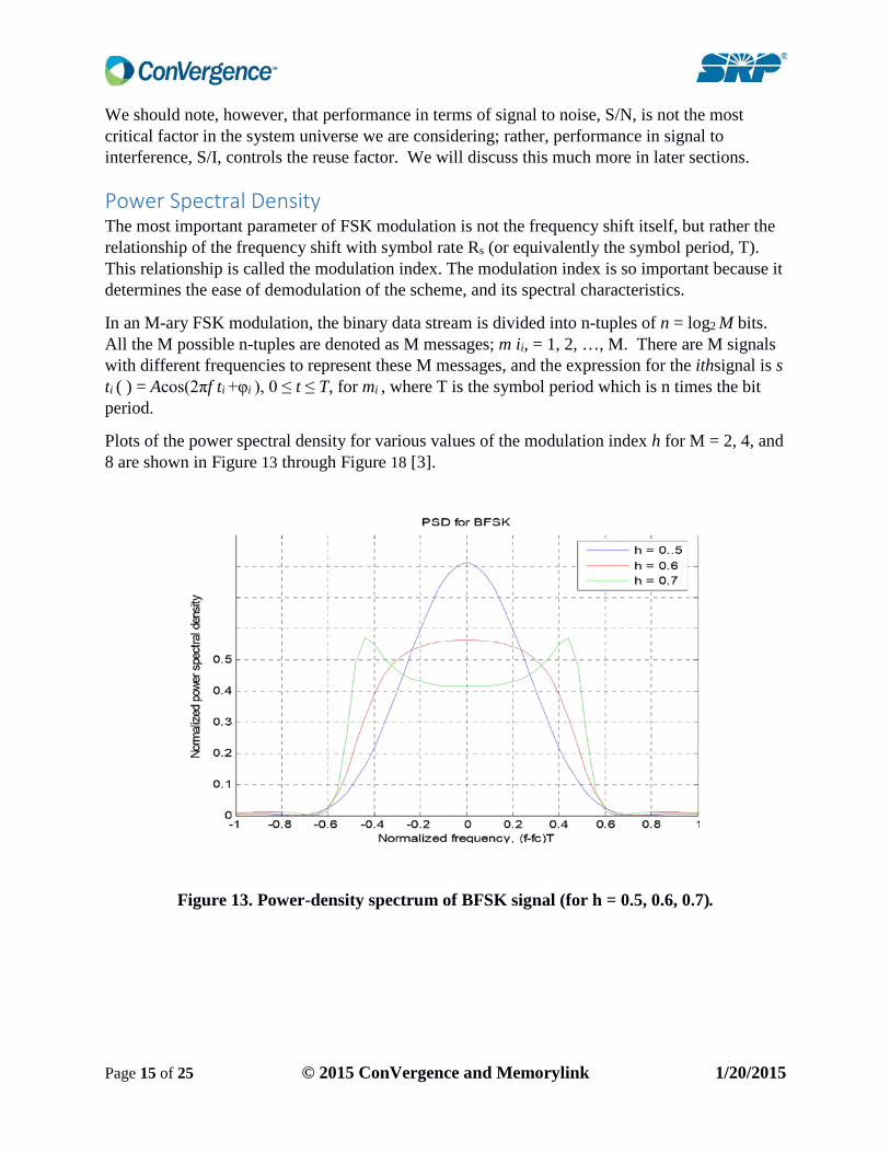
Power Spectral Density The most important parameter of FSK modulation is not the frequency shift itself, but rather the relationship of the frequency shift with symbol rate Rs (or equivalently the symbol period, T). This relationship is called the modulation index. The modulation index is so important because it determines the ease of demodulation of the scheme, and its spectral characteristics.

In an M-ary FSK modulation, the binary data stream is divided into n-tuples of n = log2 M bits. All the M possible n-tuples are denoted as M messages; m ii, = 1, 2, …, M. There are M signals with different frequencies to represent these M messages, and the expression for the ithsignal is s ti ( ) = Acos(2πf ti +φi ), 0 ≤ t ≤ T, for mi , where T is the symbol period which is n times the bit period.

Plots of the power spectral density for various values of the modulation index h for M = 2, 4, and 8 are shown in Figure 13 through Figure 18 [3].

Figure 13. Power-density spectrum of BFSK signal (for h = 0.5, 0.6, 0.7).


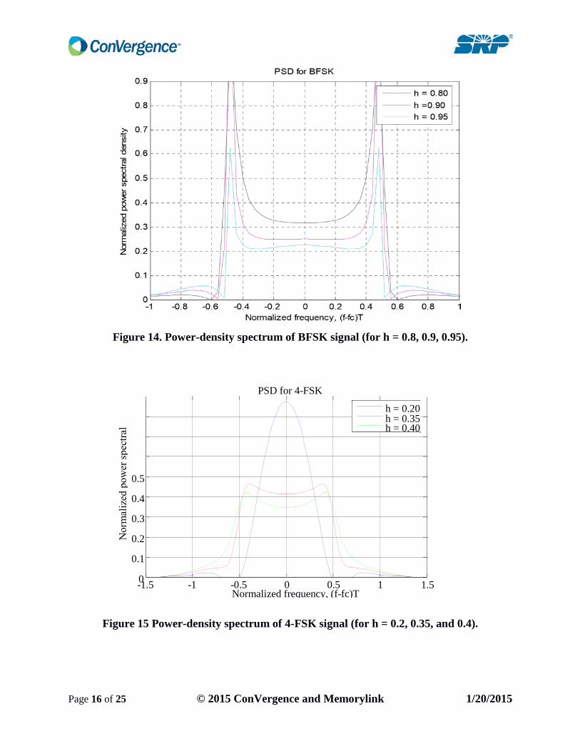
Figure 14. Power-density spectrum of BFSK signal (for h = 0.8, 0.9, 0.95).

Figure 15 Power-density spectrum of 4-FSK signal (for h = 0.2, 0.35, and 0.4).

-1.5 -1 -0.5 0 0.5 1 1.5 0

0.1

0.2

0.3

0.4

0.5

Normalized frequency, (f-fc)T

PSD for 4-FSK

h = 0.20 h = 0.35 h = 0.40


Figure 16. Power-density spectrum of 4-FSK signal (for h = 0.5, 0.6, and 0.7).




Curves are presented for various values of h to show how the spectral shape changes with h. For small values of h, the spectra are narrow and decrease smoothly towards zero. As h increases towards unity, the spectrum widens and spectral power is increasingly concentrated around -0.5 ≤ (f – fc) ≤ 0.5 and its odd multiples. These are the frequencies of the M signals in the scheme.

For coherent orthogonal case, h = 0.5 (Figure 3.29), most spectral components are in a bandwidth of M/2T. Thus the transmission bandwidth is set as BT = M/2T. Similarly, for noncoherent orthogonal case, h = 1, and then BT = M/T.

-3 -2 -1 0 1 2 3 0

0.05

0.1

0.15

0.2

0.25

Normalized frequency, (f-fc)T

PSD for 8-FSK

h = 0.4 h = 0.5 h = 0.6


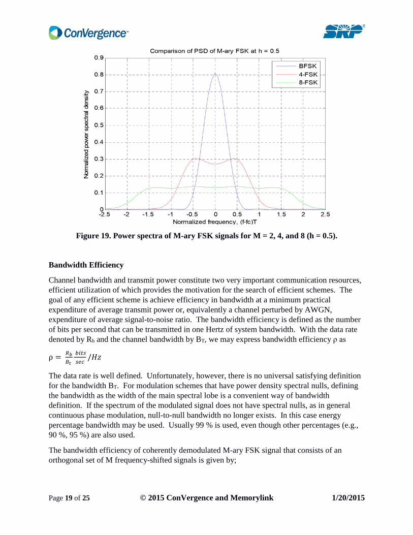
Figure 19. Power spectra of M-ary FSK signals for M = 2, 4, and 8 (h = 0.5).

Bandwidth Efficiency

Channel bandwidth and transmit power constitute two very important communication resources, efficient utilization of which provides the motivation for the search of efficient schemes. The goal of any efficient scheme is achieve efficiency in bandwidth at a minimum practical expenditure of average transmit power or, equivalently a channel perturbed by AWGN, expenditure of average signal-to-noise ratio. The bandwidth efficiency is defined as the number of bits per second that can be transmitted in one Hertz of system bandwidth. With the data rate denoted by Rb and the channel bandwidth by BT, we may express bandwidth efficiency ρ as

ρ = 𝑅𝑅𝑏𝑏𝐵𝐵𝑡𝑡

𝑏𝑏𝑏𝑏𝑏𝑏𝑏𝑏𝑏𝑏𝑠𝑠𝑠𝑠

/𝐻𝐻𝐻𝐻

The data rate is well defined. Unfortunately, however, there is no universal satisfying definition for the bandwidth BT. For modulation schemes that have power density spectral nulls, defining the bandwidth as the width of the main spectral lobe is a convenient way of bandwidth definition. If the spectrum of the modulated signal does not have spectral nulls, as in general continuous phase modulation, null-to-null bandwidth no longer exists. In this case energy percentage bandwidth may be used. Usually 99 % is used, even though other percentages (e.g., 90 %, 95 %) are also used.

The bandwidth efficiency of coherently demodulated M-ary FSK signal that consists of an orthogonal set of M frequency-shifted signals is given by;


𝜌𝜌 = 𝑅𝑅𝑏𝑏𝑀𝑀2𝑇𝑇

𝑏𝑏𝑏𝑏𝑏𝑏𝑏𝑏𝑏𝑏𝑠𝑠𝑠𝑠

/𝐻𝐻𝐻𝐻 Equation 1

where Rb is the data rate in bits per second, and T is the symbol period which is n times the bit period.

Table 2 gives the values of ρ calculated from Equation 1 for M = 2, 4, 8, and 16.

M 2 4 8 16

ρ

(bits/s/Hz)

1.0 1.0 0.75 0.50

Table 2. Bandwidth Efficiency of M-FSK

Performance in Interference Again, note carefully that the above discussion covers only S/N performance in a single cell. The most important point is the signal to interference performance. For convenience we will refer to this parameter as SJR in future, and to signal to noise, S/N, as SNR.

The beginning of this discussion is explored in Figure 20 below. Each of the various lines represents a different fixed level of SNR. 10 levels of SNR are shown, ranging from -5 dB to +12 dB in steps of 1.89 dB. The solid line, which looks like a step function, is the probability of bit error when only interference is present. Note that it changes abruptly from 0.5 (guessing!) to essentially zero at 0 dB signal to interference (SJR).

Figure 20. Performance in Interference and Noise of 2-FSK.


A similar set of curves is show in Figure 21 for 4-FSK, and in Figure 22 for 8-FSK. Note that the signal to interference ratio for zero error moves to the left, toward poorer signal, as the bits per symbol increases.




Figure 23 below shows the interference-only situation for 2-, 4-, and 8-FSK. Note that the Signal to Interference performance of 8-FSK is -4.5 dB; in strong signal areas, it shows very low bit error rate when the interference is almost 3 time stronger than the signal!

Figure 23. Performance in Interference Only of 2-, 4-, and 8-FSK With this level of performance in interference, the use of omnidirectional antennas on the client units would be quite practical, although in some circumstances it would limit reuse to a degree, as some coordination between nearby users in different cell/sectors would be required.

Overall Spectral Efficiency As the above discussion shows, using 8-FSK will give a bandwidth efficiency in any one sector of any one cell of .75 while allowing us to meet the FCC limit of -43 dBw at the edges of the 1-MHz band segments, corresponding to a peak data rate to any one point of up to 750 Kbps. If more peak throughput is required, it would be quite practical to include a “turbo” mode utilizing OFDM and multi-level QAM, allowing data rates of at least several megabits, albeit with considerable poorer interference performance and therefore poorer reuse.

This can be said to correspond to a “guard band” of about 125 KHz at each edge. To take a further look at this, go to Figure 17 and examine the curve for h = 0.2; it shows the energy falling to zero at plus and minus 1.5 times the symbol rate 1/T. This implies that the occupied bandwidth by the 1% rule is 3 times the symbol rate. For 700 Kbps throughput with 8-FSK, the symbol rate is of course 700/3=233.3 symbols/sec, and occupied bandwidth is 3 times that, or 700 KHz, leaving a “guard band” of 150 KHz at each edge of the 1-MHz spectrum slice.

The precise symbol rate (and therefore throughput) is certainly between 700 and 800 Kbps; finer resolution depends on details of the final equipment design, which can be expected to be somewhat better than that used in the tests described in this document.

To summarize the overall throughput, we have shown that using 8-FSK, throughput is ~700 K bps per frequency per cell-sector; 4 sectors per cell are easy, and we can use as many cells as desired, giving essentially unlimited total system throughput. Using both spectrum slices on each sector, this gives a per-

1.00E-08

1.00E-07

1.00E-06

1.00E-05

1.00E-04

1.00E-03

1.00E-02

1.00E-01

1.00E+00

-7 -6 -5 -4 -3 -2 -1 0 1 2 3 4 5 6 7 8

Bit E

rror

Rat

e

Signal to Interference

2-FSK 4-FSK 8-FSK


cell site throughput of 2 x 4 x 700 Kbps, or 5.6 Mbps/cell site, but the individual max streaming rate is still 700 Kbps. We can add a turbo mode of ~5 Mbps, but the total throughput for the cell will not increase, and that of neighboring cells may well fall as well. Thus the coordination problem introduced by using modulation technology with poorer performance in interference.

Network and Control Layer One of the key characteristics of the SRP application is the preponderance of uplink data; that is, information flow from client units to the Access Points. The initial data from SRP indicates a 20/80 split in favor of uplink traffic. A frequency-division duplex approach would therefore leave 30% of the total available throughput on the table.

Further, the necessity of coordinating (automatically) with nearby LTE cell sites is made much easier by the availability of a second frequency, as is described later in this paper.

Another important consideration is that of providing a mechanism for client units to reach Access Points that they may not be able to reach directly, due to such things as terrain. Perhaps the most practical way to provide that capability is through a mesh network.

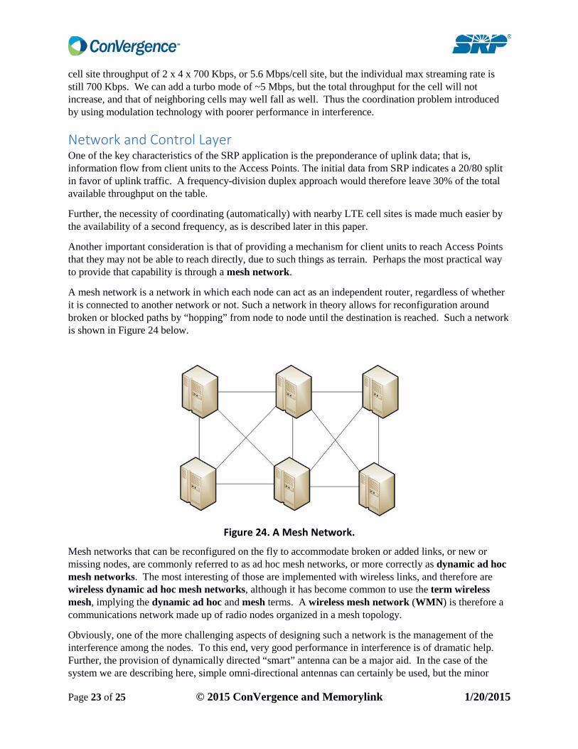
A mesh network is a network in which each node can act as an independent router, regardless of whether it is connected to another network or not. Such a network in theory allows for reconfiguration around broken or blocked paths by “hopping” from node to node until the destination is reached. Such a network is shown in Figure 24 below.

Figure 24. A Mesh Network.

Mesh networks that can be reconfigured on the fly to accommodate broken or added links, or new or missing nodes, are commonly referred to as ad hoc mesh networks, or more correctly as dynamic ad hoc mesh networks. The most interesting of those are implemented with wireless links, and therefore are wireless dynamic ad hoc mesh networks, although it has become common to use the term wireless mesh, implying the dynamic ad hoc and mesh terms. A wireless mesh network (WMN) is therefore a communications network made up of radio nodes organized in a mesh topology.

Obviously, one of the more challenging aspects of designing such a network is the management of the interference among the nodes. To this end, very good performance in interference is of dramatic help. Further, the provision of dynamically directed “smart” antenna can be a major aid. In the case of the system we are describing here, simple omni-directional antennas can certainly be used, but the minor


added complexity (with today’s technology) needed for “smart” antennas seems to be well worth the effort.

It should be noted that there is no reason that the two approaches cannot be mixed – start with simple omni antenna, and then add newer units with “smart” antenna technology as the products evolve.

Summary This document reports on the theoretical and real-world performance of a digital system that is specifically focused on meeting the needs of data acquisition and control for a major public utility, operating in the 2 by 1 MHz segments made available for non-traditional services in the 700 MHz A-block spectrum.

It is clear that a 2-frequency repeat pattern (or 2 time slots) in the downlink direction will easily suffice to guarantee reception to a very high probability by all client units, and further that uplink messages will be received to an even higher probability as long as all access points can receive any client module. In fact, most of the area will allow one-frequency reuse, and the equipment can easily made capable of determining the appropriate frequency and therefore reuse pattern for any given link. This means that the ultimate system can easily have a throughput capability of 400 to 500 thousand bits/sec per cell, with most of the cell having twice that capacity. Along with the ability to make cells as small as desired, this results in a virtually infinite total throughput capability. In short, there is no practical limit to overall system throughput, only in peak data rate to any one point.

We consider the subject spectrum to be quite suitable for the use that SRP proposes.

References

[1] T.A. Freeburg, The Cellular Transformation, internal paper, Sept. 1993

[2] M. Hata, Emperical formula for propagation loss in land mobile radio services, IEEE Trans., VT 29 No. 3 (1980)

[3] Eric Nii Otorkunor Sackey, Performance Evaluation of M-ary Frequency Shift Keying Radio Modems, Department of Electrical Engineering, Blekinge Institute of Technology, Karlskrona, Sweden, September 2006

[4] Kyle Cormier, SRP Bandwidth Requirements Info, SRP internal document

[5] Kenneth C. Budka, Estimating Smart Grid Communication Network Traffic, Bell Labs/Alcatel-Lucent Internal Report, March 17, 2014


Appendix 1. Raw Field Test Data.

Name Lat Long

Distance from PBF, Miles analyzer

error rate comments

srp 05 33.43953 111.9457 0.33 -55 0 very strong srp 06 33.43951 111.9458 0.33 -48 0 very strong srp 07 33.4379 111.9513 0.61 -80 0.05 see multipath on analyzer; peaks are -93 and -80 srp 07 a 33.4379 111.9513 0.61 -74 0 Move another 50 feet srp 08 33.44275 111.9558 0.74 -80 0 some multipath visible on analyzer srp 09 33.4453 111.9539 0.66 -65 0.05 srp 10 33.44585 111.9621 1.07 -85 0.1 srp 11 33.44644 111.9614 1.04 -67 0.05 srp 12 33.44698 111.9778 1.86 -85 0.05 multipath visible peaks of spectrum at 95 and 85 srp 13 33.4788 111.9815 2.94 -90 0.08 srp 13 a 33.4788 111.9815 2.94 -90 0.08 behind buildings and trees srp 14 33.42189 111.9836 2.49 -85 User error in taking reading srp 15 33.42228 111.9607 1.6 -84 User error in taking reading srp 16 33.43092 111.9429 0.75 -58 0 srp 17 33.42762 111.9679 1.64 -81 0 srp 18 33.42324 111.9566 1.44 -88 0.02 srp 18 a 33.42324 111.9566 1.44 -88 0.08 Move 1 foot srp 18 b 33.42324 111.9566 1.44 -82 0.06 Move 1 foot srp 18 c 33.42324 111.9566 1.44 -87 0.08 Move 1 foot srp 18 d 33.42324 111.9566 1.44 -80 0.04 Move 1 foot srp 18 e 33.42324 111.9566 1.44 -85 0.08 Move 1 foot srp 19 33.42323 111.9484 1.26 -88 0.01 srp 21 33.42214 111.986 2.59 -95 0.08 srp 22 33.42229 111.9947 2.97 -96 0.02 srp 23 33.416 112.0088 3.77 -96 0.15 spatial average ~35% coverage


salt river project 700 mhz draft report - utc

Documents