Discussion

Paper

|D

iscussionP

aper

|D

iscussionP

aper|

Discussion

Paper

|

Ocean Sci. Discuss., 12, 983–1011, 2015www.ocean-sci-discuss.net/12/983/2015/doi:10.5194/osd-12-983-2015© Author(s) 2015. CC Attribution 3.0 License.

This discussion paper is/has been under review for the journal Ocean Science (OS).Please refer to the corresponding final paper in OS if available.

Regime changes in global sea surfacesalinity trend

A. L. Aretxabaleta1,*, K. W. Smith2, and J. Ballabrera-Poy1

1Institut de Ciències del Mar – CSIC, Barcelona, Spain2Independent Research, West Tisbury, MA, USA*now at: US Geological Survey and Integrated Statistics, Woods Hole, MA, USA

Received: 9 April 2015 – Accepted: 11 May 2015 – Published: 3 June 2015

Correspondence to: A. L. Aretxabaleta (aaretxabaleta@usgs.gov)

Published by Copernicus Publications on behalf of the European Geosciences Union.

983

Discussion

Paper

|D

iscussionP

aper|

Discussion

Paper

|D

iscussionP

aper|

Abstract

Recent studies have shown significant sea surface salinity (SSS) changes at scalesranging from regional to global. In this study, we estimate global salinity means andtrends using historical (1950–2014) SSS data from the UK Met. Office Hadley Centreobjectively analyzed monthly fields and recent data from the SMOS satellite (2010–5

2014). We separate the different components (regimes) of the global surface salinityby fitting a Gaussian Mixture Model to the data and using Expectation–Maximizationto distinguish the means and trends of the data. The procedure uses a non-subjectivemethod (Bayesian Information Criterion) to extract the optimal number of means andtrends. The results show the presence of three separate regimes: Regime A (1950–10

1990) is characterized by small trend magnitudes; Regime B (1990–2009) exhibitedenhanced trends; and Regime C (2009–2014) with significantly larger trend magni-tudes. The salinity differences between regime means were around 0.01. The trendacceleration could be related to an enhanced global hydrological cycle or to a changein the sampling methodology.15

1 Introduction

Global sea surface salinity (SSS) is changing at scales ranging from regional to global(Antonov et al., 2002; Boyer et al., 2005). Global salinity reflects the balance betweensurface freshwater flux (evaporation minus precipitation), terrestrial runoff, and mix-ing and advective processes in the ocean. Thus, changes in salinity are intrinsically20

connected to alterations in the global hydrological cycle and are expected to be a con-sequence of climate change (Held and Soden, 2006). The intensification of the globalwater cycle is expected to be occurring at a rate of 8 %degree−1 of surface warming(Durack et al., 2012) or around 20 % considering the projected 2–3 ◦ of temperatureincrease over the next century.25

984

Discussion

Paper

|D

iscussionP

aper

|D

iscussionP

aper|

Discussion

Paper

|

Recently, Antonov et al. (2002) and Boyer et al. (2005) described a general changepattern with surface subtropical areas becoming saltier and high-latitude regions be-coming fresher. Curry et al. (2003) found increased salinity in the subtropical evaporation-dominated regions between 25◦ S and 35◦N when they compared the time periods1955–1969 and 1985–1999 for the entire Atlantic basin. Cravatte et al. (2009) de-5

scribed a large freshening in the Pacific warm pool over the 1955–2003 period.Hosoda et al. (2009) analyzed global surface salinity comparing Argo float data for

the period 2003–2007 with climatological 1960–1989 data from the 2005 World OceanDatabase. The recent Argo data showed lower salinities in fresher regions and highersalinities in areas of higher salinity magnitudes. They linked the changes to increased10

global hydrological cycle during the 30 years between their observations.Durack and Wijffels (2010) (DW10 herein) analyzed data for the period 1950–2008

and found SSS increases in regions dominated by evaporation while freshening oc-curred in precipitation-dominated regions. They suggested the change was a conse-quence of an intensification of the global hydrological cycle. They also provided a com-15

prehensive review of salinity changes in the literature. Using a linear fit for the 1950–2008 data, DW10 found that in a 50 year period, the subtropical gyres (evaporationdominated) exhibited net salinity increases from 0.20 in the eastern south pacific to0.45 in the subtropical north Atlantic. During the same period, the salinity decreased inthe precipitation-dominated regions (for instance, under the Intertropical Convergence20

Zone, ITCZ), with decreases ranging from −0.25 in the Equatorial Atlantic to −0.57 inthe western Equatorial Pacific.

The SSS spatial pattern has been associated with the “rich get richer” mechanismfor evaporation-precipitation (Chou et al., 2009). In fact, the enhancement in hydrolog-ical cycle has been studied based on the changes in ocean salinity (Schmitt, 2008;25

Helm et al., 2010; Durack et al., 2012; Durack, 2015). The intensification of the watercycle was larger over 1979–2010 than in earlier periods (1950–1978) related to theaccelerated broad-scale warming (Skliris et al., 2014).

985

Discussion

Paper

|D

iscussionP

aper|

Discussion

Paper

|D

iscussionP

aper|

The determination of a single SSS trend by DW10 highlighted significant challenges(e.g., data deficiencies in some regions and times), but it represented only a first steptoward a characterization of the time evolution of global salinity. The results of recentanalyses of other ocean parameters, such as water level (Church and White, 2006;Ezer, 2013), have demonstrated that changes in the ocean have been accelerated in5

recent times. In some regions, the rate of change of the water level time series exceedseven a quadratic fit over at least the last 50 years (Church and White, 2006). In fact, therole of salinity on water level changes has also been recently explored (Durack et al.,2014).

The question we are trying to address in this study is whether the SSS changes are10

due to: (1) a regime shift in which the SSS has moved from one equilibrium state toanother (maybe even several regime shifts), (2) a constant SSS trend (no new equilib-rium has been achieved), (3) a varying SSS trend (not only is SSS changing, but therate of change varies); or (4) a combination of the above.

In this study, we separate the different regimes (components with substantially differ-15

ent characteristics) of the global SSS (1950–2014) by fitting Gaussian Mixture Models(GMM) with and without trends to the SSS data to characterize, not only the means,but also the trends. The GMMs are estimated using an Expectation–Maximization al-gorithm with the number of components determined non-subjectively by the BayesianInformation Criterion to extract the optimal number of means and trends. The long-term20

global SSS dataset from the UK Met. Office Hadley Centre (Good et al., 2013) is cho-sen as the reference data source. Recently available SMOS satellite data is used asa complement for the period 2010–2014.

986

Discussion

Paper

|D

iscussionP

aper

|D

iscussionP

aper|

Discussion

Paper

|

2 Data and methods

2.1 Long-term global salinity data

The Met Office Hadley Centre provides global quality controlled ocean temperatureand salinity profiles and monthly long-term objectively analyzed global fields with a onedegree spatial resolution (Ingleby and Huddleston, 2007; Good et al., 2013). The most5

recent EN4 dataset includes objectively analyzed fields formed from profile data withuncertainty estimates. The available data extend from 1900 to the present and thereare separate files for each month. Good et al. (2013) used a simple Analysis Correc-tion (Lorenc et al., 1991) optimal interpolation methodology to analyze global historicalobservations that had been methodically quality controlled. The analysis fields were10

constructed by combining a background field (the analysis field of the previous month)with the quality controlled profiles from the month being analyzed.

In this work, the surface salinity field (top layer of the dataset) from 1950 to 2014 isused. The 1950 cutoff was chosen to match previous trend studies (Boyer et al., 2005;Durack and Wijffels, 2010) and to prevent data-deficient periods.15

2.2 SMOS satellite data

The recently available SMOS (Soil Moisture and Ocean Salinity) satellite (Font et al.,2010, 2012) provides sea surface salinity data with sufficient spatial resolution (1/4◦)to characterize global (Xie et al., 2014) and regional (e.g., Amazon: Aretxabaleta andSmith, 2013; North Atlantic SSS maximum: Hernandez et al., 2014; Kolodziejczyk20

et al., 2015; Gulf Stream: Reul et al., 2014; northern North Atlantic: Köhler et al., 2015)features. Recently, SMOS data have been used to study salinity variability in the At-lantic (Tzortzi et al., 2013), the signature of La Niña in the tropical Pacific Ocean (Has-son et al., 2014) and even create surface T/S diagrams (Sabia et al., 2014). Level 3(global maps) data were obtained from the CP34 distribution center at the SMOS25

Barcelona Expert Centre (http://tarod.cmima.csic.es) for the period 2010–2014. The

987

Discussion

Paper

|D

iscussionP

aper|

Discussion

Paper

|D

iscussionP

aper|

temporal resolution of the objectively analyzed SMOS data is one month and the spa-tial resolution is 1/4◦. We averaged the data to one degree resolution to match thelong-term dataset and reduce noisy signals.

The SMOS satellite data exhibited deficiencies near coastal areas and in high lati-tudes (Guimbard et al., 2012; Yin et al., 2014; Hernandez et al., 2014; Köhler et al.,5

2015). To prevent the introduction of bogus features, those data were removed fromthe analysis. The main areas affected were in high latitudes, in the proximity of conti-nents, the Mediterranean, and in a large area of the western Pacific surrounding thePhilippines and Japan.

2.3 Gaussian mixture models and expectation-maximization10

A Gaussian Mixture Model (GMM) is a probabilistic model for which the probability den-sity function is a combination of two or more Gaussian distributions. The Expectation–Maximization (EM) algorithm is an iterative procedure to find a Maximum LikelihoodEstimate (MLE) of the parameters of a GMM. In the past, the EM algorithm was usedto separate the regimes of a spatial time series (Smith and Aretxabaleta, 2007) and to15

find the best GMM describing the joint distribution of model and data in a model skill as-sessment scenario (Aretxabaleta and Smith, 2011). In previous studies, EM was usedto estimate missing values for oceanographic datasets (Houseago-Stokes and Chal-lenor, 2004; Kondrashov and Ghil, 2006). Aretxabaleta and Smith (2013) introduceda measurement operator (H) and error (assuming the observations were unbiased20

with a Gaussian measurement error ε(t) ∼ G(0,R(t)) of known covariance, R(t)), toprovide a more general algorithm that could be used for missing data and interpolationproblems.

In this implementation, we introduce the possibility of defining the GMM by botha mean and a linear temporal trend. After we have found the number of components25

(representing probability density functions), nc, component distributions (mean, trend,and covariance), G(µk ,αk ,Σk), and their respective likelihoods, τk , we can conduct anEmpirical Orthogonal Function (EOF) analysis on the Σk .

988

Discussion

Paper

|D

iscussionP

aper

|D

iscussionP

aper|

Discussion

Paper

|

Let d (t) denote a set of time series with a linear measurement operator, H(t), froma spatial basis on which we want to estimate the state ψ(t) at all time points, such thatd (t) = H(t)ψ(t)+ε(t). We fit a mixture model to the data set, ψ . For an nc componentGaussian mixture model, we have in general

p(ψ |µ1, . . .µnc ,α1, . . .αnc ,Σ1, . . .Σnc ,τ1, . . .τnc)5

=nc∑

k=1

τkexp(−1

2 (ψ −µk −αkt)T [Σk ]−1(ψ −µk −αkt))√

(2π)2nd |Σk |, (1)

where nd is the spatial dimension of ψ , τk is the probability of component distributionk, and µk , αk , and Σk are the mean, trend, and covariance of the kth componentdistribution. |Σk | is the determinant of the covariance.

The two steps of the EM iterative procedure are:10

Expectation step: For each time point, t, in the dataset, the expected value for compo-nent k of the likelihood function, wk(t), is calculated under the current estimate of theparameters µk (mean), αk (trend), and Σk (covariance):

wk(t) =

exp[ (− 1

2 (d (t)−H(t)(µk +αkt))T [H(t)ΣkH(t)T +R(t)]−1(d (t)−H(t)(µk +αkt))

)]

√(2π)nd |H(t)ΣkH(t)T +R(t)|

. (2)

Then, the likelihoods are normalized,15

wk(t)→ wk(t)∑jw j (t)

. (3)

Maximization step: The optimal parameters that maximize the current estimate giventhe data d (t) are calculated. Note that τk , µk , αk , and Σk may all be maximized inde-pendently of each other since they appear in separate linear terms. The frequency of

989

Discussion

Paper

|D

iscussionP

aper|

Discussion

Paper

|D

iscussionP

aper|

the kth component distribution, nk =∑tw

k(t), is computed and normalized,

τk =nk

nt=

∑tw

k(t)

nt, (4)

where nt is the length of the time series.

We enforced that the time series is an autoregressive process of order one (AR(1)) toavoid rapid switching between regimes. Thus, the salinity at time t depends linearly on5

the previous value, d (t) = c+ϕd (t−1)+εt, where c is a constant, ϕ is the parameterof the AR(1) model and εt is white noise.

An EOF analysis can be conducted based on the component distributions covari-ances, Σk . Using the eigenvectors of Σk , we obtain a new set of orthogonal basisfunctions that are meaningful for times when wk(t) ' 1. The EOF analysis can be con-10

sidered independently during different regimes in a similar approach to Tipping andBishop (1999).

Our approach is related to the multivariate adaptive regression splines (MARS) method(Friedman, 1991) as both automatically determine the number and timing of the sepa-ration between regimes (breakpoints or knots) based on the data. The main difference15

between the two approaches is that our method includes multiple spatial location (mul-tiple time series) and the regime extraction is across the complete dataset.

2.4 Non-subjective choice of number of regimes: Bayesian InformationCriterion

To determine the optimal number of components (regimes) in the GMM, we use the20

Bayesian Information Criterion (BIC, Schwarz, 1978; Aretxabaleta and Smith, 2011).The BIC is an empirical approach that approximates the total probability (Bayes factor)of a probability distribution under some set data,

BIC(k) = −2log(p̂(ψ |µ1, . . .,µnc ,α1, . . .,αnc ,Σ1, . . .,Σnc ,τ1, . . .,τnc))−Dk log(nt). (5)990

Discussion

Paper

|D

iscussionP

aper

|D

iscussionP

aper|

Discussion

Paper

|

The penalty term preventing over-fitting, Dk , for a GMM with nc components and ntime series is Dk = ncn(n+2)/2+nc−1, where ncn of those are for the means of eachdistribution, another ncn correspond to the trends, ncn(n−1)/2 are for the parametersof the covariance matrix, and nc −1 for the τk .

There are a number of potential combinations of means and trends (Fig. 1) that5

can be fitted to any spatial time series. In the current application, the Expectation–Maximization (EM) algorithm is used to find the best GMM describing the data distribu-tion. The method is run under several possible scenarios that separate regimes basedon including only means, means and a global trend, and a combination of means andtrends. The BIC approach penalizes excessive number of parameters with Dk being ad-10

justed depending on the inclusion/exclusion of trends. BIC is used twice in the currentprocedure: first, to choose the optimal number of components in a particular scenario(e.g., only means, combining means and trends), and second, to choose among thedifferent scenarios.

3 Results15

3.1 Comparison with DW10

The Hadley Centre EN4 surface salinity interpolated fields incorporated quality con-trolled observations in a similar manner as the database used by Durack and Wijffels(2010) to create the DW10 surface fields. DW10 fields were reported for a 50 year pe-riod (nominally 1950–2000) to simplify comparisons, even though they used data from20

1950 to 2008. To establish whether the datasets were sufficiently similar, we calculatedthe mean and trend for the same period as DW10 (1950–2008) using the interpo-lated data (Fig. 2). The climatological mean surface salinity (Fig. 2a) exhibits the samegeneral structure and magnitude as the DW10 results.The standard deviation of thesurface salinity (Fig. 2b) highlights the increased variability associated with river dis-25

charge, the ITCZ, and intense meandering current systems like the Gulf Stream. As in

991

Discussion

Paper

|D

iscussionP

aper|

Discussion

Paper

|D

iscussionP

aper|

the case of the mean, the 50 year linear surface salinity trend (Fig. 2c) is also similarto the published fields with minimal differences. For instance, there is a slightly lessnegative trend in the Equatorial and North Atlantic and a larger positive trend in theAntarctic Circumpolar Current region in our results. Overall, the trend magnitude andspatial distribution for the 1950–2008 period are equivalent in both datasets. The main5

trend features include a predominantly positive trend in the Atlantic, southeastern Pa-cific, and Indian Ocean, and a predominantly negative trend in the north and westernPacific and along the Antarctic Circumpolar Current region.

3.2 Regime separation using Hadley Centre EN4 1950–2014 fields

When the global SSS monthly data from the Hadley Centre EN4 were analyzed, the10

EM method distinguished three separate regimes. These regimes are characterizedby different means but also different trends (Figs. 3 and 4). The separation (break-point) between the first two regimes (Regime A and B) occurs in May 1990, while theseparation between the second and third regimes (Regime B and C) was found to beMarch 2009.15

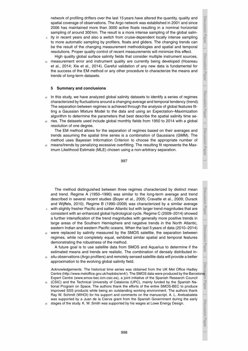
The global surface salinity means for the three regimes (Fig. 3) exhibited the samegeneral pattern with higher salinity in the subtropical gyres and lower values in the sub-polar, polar regions, and under the ITCZ. The differences between regime means wereon the order of 0.1 (0.099 rms difference between Regime A and B; and 0.15 betweenRegime B and C). The Regime B (1990–2009) average was saltier than Regime A20

(1950–1990) in most of the Atlantic Ocean except along the eastern US, in the centralequatorial region, and south of 30◦ S. In contrast most of the Pacific (except for thesouthwest) was fresher in Regime B than A. The difference between the average salin-ities of Regime B (1990–2009) and Regime C (2009–2014) exhibited saltier values inthe later period in most of the Pacific and South Atlantic, while a large part of the North25

Atlantic was fresher during Regime C.The trend for Regime A (1950–1990, Fig. 4a) was consistent with the results ob-

tained by DW10 (Durack and Wijffels (2010) and Fig. 2, note the different scale) and992

Discussion

Paper

|D

iscussionP

aper

|D

iscussionP

aper|

Discussion

Paper

|

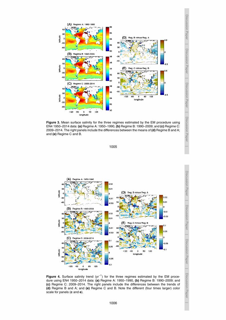
the references therein. The differences were a slightly larger positive trend in the Equa-torial Atlantic and a lack of positive trend in the eastern Pacific. The trend for Regime B(1990–2009, Fig. 4b) exhibited larger positive magnitudes in the North and South At-lantic than Regime A, a negative trend (∼ −0.02 yr−1) along the Equatorial Atlantic,negative trends in the areas of the Antarctic Circumpolar Current and positive trends5

(0.01–0.02 yr−1) in most of the Pacific between 30◦ S and 30◦N. The trend associatedwith Regime B exhibited enhanced magnitudes when compared to Regime A (positivetrends were more positive and negative areas were more negative during Regime B).In both regimes the trends are consistent with an intensification of the global hydro-logical cycle (Schanze et al., 2010; Yu, 2011). The estimated trend during Regime C10

(2009–2014, Fig. 4c) was much larger than in any of the two early regimes. TheRegime C trend was negative in the majority of the North Atlantic (up to −0.04 yr−1),eastern Indian Ocean (∼ −0.05 yr−1) and western (< −0.05 yr−1) and south equatorial(∼ −0.03 yr−1) Pacific. Positive trends during Regime C were estimated along the west-ern part of the Equatorial and South Atlantic (up to 0.06 yr−1), the Pacific subtropical15

gyres (ranging 0.02–0.05 yr−1) and the western Indian Ocean (∼ 0.04 yr−1).The salinity time evolution showed the changing temporal pattern during the full

record and the potential distinction between regimes (Fig. 5). For instance, the Equato-rial Atlantic (Fig. 5a, 5◦ S–5◦N) showed a notable difference between the trends for thethree regimes, while the difference between the average salinity of the three regimes20

was small. The North Atlantic Subtropical Gyre (Fig. 5b, 15–30◦N) in contrast exhib-ited noticeable differences in the trends, but especially in the means between the threeregimes. Meanwhile, the most striking feature in the Mediterranean (Fig. 5c) and in theEquatorial Pacific (Fig. 5d, 5◦ S–5◦N) was the sharp drop in salinity associated withEl Niño events while the main difference between regimes was again in the magni-25

tude of the trend. The largest trend acceleration between regimes was present in theMediterranean (Fig. 5c).

As described in Sect. 2.3, the EM algorithm also allowed for the separation of themodes of variability. The 1st EOF for Regime A and B explained over 75 % of the vari-

993

Discussion

Paper

|D

iscussionP

aper|

Discussion

Paper

|D

iscussionP

aper|

ance (79 and 77 %, respectively) while only explaining 67 % of the Regime C variance.Meanwhile, the 2nd EOF explained 11, 12 and 14 % of the variance in each regime.The 1st EOF of Regime A was spatially consistent with Regime B, but its magnitudewas smaller (Fig. 6). The 1st EOF in the first two regimes suggested the Atlantic andsoutheastern Pacific were fluctuating in phase, while the western Pacific and most of5

the Southern Ocean were out of phase. The 1st EOF of Regime C exhibited a differentspatial pattern and larger magnitude with the separation between basins being less ap-parent, with the main feature likely associated with the northern/southern migration andextent of the ITCZ. The 2nd EOF for the first two regimes was quite similar with positivevalues in most areas except the Antarctic and Equatorial Pacific oceans. Meanwhile,10

the 2nd EOF of Regime C was mostly consistent with the Pacific and Atlantic oceansbeing out of phase. The time series of the 1st EOF (Fig. 7a) showed larger short-termfluctuations for Regime B and Regime C, with Regime B exhibiting a trend in time.There was an apparent relationship between the 2nd EOF for Regime B (Fig. 7b) andthe ENSO cycle (1998, 2003, 2005 peaks), while no clear relation appeared to be15

present for Regime A or C.

3.3 Regime separation with updated SMOS fields 2010–2014

The recent availability of global surface salinity fields from satellites (SMOS and Aquar-ius) provided the possibility of using alternative data that were not included as part ofthe Good et al. (2013) dataset. The goal was to analyze the robustness of the regime20

separation by replacing the recent (2010–2014) fields with satellite-derived products.The inclusion of the available 5 years of SMOS data in the analysis in substitution of

the EN4 data for 2010–2014 slightly altered the EM separation results (Figs. 8 and 9).The EM method also distinguished three separate regimes (A’, B’, and C’) with differentmeans and trends. The breakpoint between Regime A’ and B’ was in July 1988 and be-25

tween Regime B’ and C’ in January 2010. The difference in the separation (breakpoint)dates between the early regimes was expected as the merged dataset did not include

994

Discussion

Paper

|D

iscussionP

aper

|D

iscussionP

aper|

Discussion

Paper

|

several areas (proximity to coastal areas, Mediterranean Sea, high latitude) that werepresent in the original EN4 dataset.

The means and differences of the two first regimes (Fig. 8a, b and d) were equivalentto the results for the complete EN4 dataset (Fig. 3). The average salinity for Regime C’(Fig. 8c) exhibited significant differences from both the Regime B’ mean and also from5

the third regime of the original dataset (Regime C, 2009–2014). The mean salinityduring Regime C’ was fresher in the North (up to −0.5) and Equatorial Atlantic, theIndian and western Pacific Oceans, while being saltier in most of the Southern Oceanand in large areas of the Pacific Ocean.

As was the case with the means, the trends of the two first regimes (A’ and B’) of10

the combined time series (Fig. 9a, b) were equivalent to the trends extracted from theoriginal dataset (Fig. 4) for Regimes A and B. The trend for Regime C’ (2010–2014,Fig. 9c) differed in magnitude and spatial structure from the trend for Regime C ofthe original EN4 dataset (2009–2014, Fig. 4c). The Regime C’ trend was positive inthe Equatorial Pacific and Atlantic while having a negative trend in most of the rest of15

the oceans with large negative values especially in the North Atlantic. The trend forRegime C’ was likely the effect of changes in the processing methodology for globalSMOS data (Guimbard et al., 2012; Yin et al., 2014).

4 Discussion

While the study focuses on the near-surface salinity, the vertical extent of the changes20

can be much larger. Boyer et al. (2005) described significant changes with varying ver-tical range depending on the basin (500 m in the Pacific, 1000 m in the Indian, and3000 m in the Atlantic Ocean). The vertical extent of the increased salinity seems to belarger than the extent in areas of freshening. The relationship between salinity and den-sity complicates the basic hypothesis of salinity changes being primarily surface forced25

(Durack and Wijffels, 2010; Durack, 2015). The combined temperature and salinity

995

Discussion

Paper

|D

iscussionP

aper|

Discussion

Paper

|D

iscussionP

aper|

changes need to be understood to explain the observed changes, especially in theinterior of the water column.

The described salinity change acceleration is likely the result of global hydrologicalcycle intensification as was suggested by Hosoda et al. (2009) and Durack and Wijffels(2010). The areas of enhanced precipitation and evaporation (Schanze et al., 2010; Yu,5

2011) correspond with the largest magnitude changes in salinity (Chou et al., 2009).The changing trend in salinity will enhance even farther the hydrological cycle intensi-fication described in Durack et al. (2012) with modifications larger than the proposed20 % in the next century.

While our most recent period (2009–2014) might be too short to be considered a ro-10

bust regime change, the differences in mean and trend between the two early regimes(A: 1950–1990; and B: 1990–2009) are consistent with the idea of salinity change ac-celeration caused by enhanced hydrological cycle. The water cycle has been shownto be farther increased in the period 1979–2010 due to accelerated warming (Skliriset al., 2014). Durack et al. (2012) analyzed modeling scenarios for the 20th century15

(Coupled Model Intercomparison Project Phase 3, CMIP3, Meehl et al., 2007) that areconsistent with not only a linear increase in hydrological cycle magnitude but also anacceleration of the intensification. The CMIP3 scenarios showed the expected intensi-fication of existing patterns of global mean E-P (“rich get richer” mechanism) and theresulting salinity pattern amplification. The changes calculated from ocean observa-20

tions were consistent with the scenario simulations but with a slightly larger effect ofglobal surface warming on salinity pattern amplification (Durack et al., 2012). The spa-tial patterns in the CMIP3 climate simulations matched the observed salinity pattern inmany areas and were consistent with the spatial structure in the present study.

As the sampling methodology and number of observations have evolved in time, the25

trend acceleration in recent times might not be a completely realistic feature. Skliriset al. (2014) suggested that while water cycle intensification was consistent with thewarming trend, it also matched the improved salinity sampling. The availability of ex-tensive field cruises in the last few decades and especially the development of the Argo

996

Discussion

Paper

|D

iscussionP

aper

|D

iscussionP

aper|

Discussion

Paper

|

network of profiling drifters over the last 15 years have altered the quantity, quality andspatial coverage of observations. The Argo network was established in 2001 and since2006 has maintained more than 3000 active floats resulting in a nominal horizontalsampling of around 300 km. The result is a more intense sampling of the global salin-ity in recent years and also a switch from cruise-dependent locally intense sampling5

to more automatic sampling by profilers, floats and gliders. The changing trends canbe the result of the changing measurement methodologies and spatial and temporalresolutions. Proper quality control of recent measurements will minimize this effect.

High quality global surface salinity fields that consider multiple instrument sources,measurement error and instrument quality are currently being developed (Hoareau10

et al., 2014; Xie et al., 2014). Careful validation of any new data is fundamental forthe success of the EM method or any other procedure to characterize the means andtrends of long-term datasets.

5 Summary and conclusions

In this study, we have analyzed global salinity datasets to identify a series of regimes15

characterized by fluctuations around a changing average and temporal tendency (trend).The separation between regimes is achieved through the analysis of global features fit-ting a Gaussian Mixture Model to the data and using an Expectation–Maximizationalgorithm to determine the parameters that best describe the spatial salinity time se-ries. The datasets used include global monthly fields from 1950 to 2014 with a global20

resolution of one degree.The EM method allows for the separation of regimes based on their averages and

trends assuming the spatial time series is a combination of Gaussians (GMM). Themethod uses Bayesian Information Criterion to choose the appropriate number ofmeans/trends by penalizing excessive overfitting. The resulting fit represents the Max-25

imum Likelihood Estimate (MLE) chosen using a non-arbitrary separation.

997

Discussion

Paper

|D

iscussionP

aper|

Discussion

Paper

|D

iscussionP

aper|

The method distinguished between three regimes characterized by distinct meanand trend. Regime A (1950–1990) was similar to the long-term average and trenddescribed in several recent studies (Boyer et al., 2005; Cravatte et al., 2009; Durackand Wijffels, 2010). Regime B (1990–2009) was characterized by a similar averagewith slightly fresher Pacific and saltier Atlantic but with larger trend magnitudes that are5

consistent with an enhanced global hydrological cycle. Regime C (2009–2014) showeda further intensification of the trend magnitudes with generally more positive trends inlarge areas of the Southern Hemisphere and negative trends in the North Atlantic,eastern Indian and western Pacific oceans. When the last 5 years of data (2010–2014)were replaced by salinity measured by the SMOS satellite, the separation between10

regimes, while not completely equal, exhibited similar spatial and temporal featuresdemonstrating the robustness of the method.

A future goal is to use satellite data from SMOS and Aquarius to determine if theestimated means and trends are realistic. The combination of densely distributed in-situ observations (Argo profilers) and remotely sensed satellite data will provide a better15

approximation to the evolving global salinity field.

Acknowledgements. The historical time series was obtained from the UK Met Office HadleyCentre (http://www.metoffice.gov.uk/hadobs/en4/). The SMOS data were produced by the BarcelonaExpert Centre (www.smos-bec.icm.csic.es), a joint initiative of the Spanish Research Council(CSIC) and the Technical University of Catalonia (UPC), mainly funded by the Spanish Na-20

tional Program on Space. The authors thank the efforts of the entire SMOS-BEC to produceimproved SSS products while being an outstanding working environment. The authors thankRay W. Schmitt (WHOI) for his support and comments on the manuscript. A. L. Aretxabaletawas supported by a Juan de la Cierva grant from the Spanish Government during the earlystages of the study. K. W. Smith was supported by his wages at Lowe Energy Design.25

998

Discussion

Paper

|D

iscussionP

aper

|D

iscussionP

aper|

Discussion

Paper

|

References

Antonov, J. I., Levitus, S., and Boyer, T. P.: Steric sea level variations during 1957–1994: im-portance of salinity, J. Geophys. Res., 107, 8013, doi:10.1029/2001JC000964, 2002. 984,985

Aretxabaleta, A. L. and Smith, K. W.: Analyzing state-dependent model-data comparison in5

multi-regime systems, Comput. Geosci., 15, 627–636, 2011. 988, 990Aretxabaleta, A. L. and Smith, K. W.: Multi-regime non-Gaussian data filling for incomplete

ocean datasets, J. Marine Syst., 119, 11–18, 2013. 987, 988Boyer, T. P., Levitus, S., Antonov, J. I., Locarnini, R. A., and Garcia, H. E.: Linear

trends in salinity for the World Ocean, 1955–1998, Geophys. Res. Lett., 32, L01604,10

doi:10.1029/2004GL021791, 2005. 984, 985, 987, 995, 998Chou, C., Neelin, J. D., Chen, C.-A., and Tu, J.-Y.: Evaluating the “rich-get-richer” mechanism in

tropical precipitation change under global warming, J. Climate, 22, 1982–2005, 2009. 985,996

Church, J. A. and White, N. J.: A 20th century acceleration in global sea-level rise, Geophys.15

Res. Lett., 33, L01602, doi:10.1029/2005GL024826, 2006. 986Cravatte, S., Delcroix, T., Zhang, D., McPhaden, M., and Leloup, J.: Observed freshening and

warming of the western Pacific warm pool, Clim. Dynam., 33, 565–589, 2009. 985, 998Curry, R., Dickson, R. R., and Yashayaev, I.: A change in the fresh-water balance of the Atlantic

Ocean over the past four decades, Nature, 426, 826–829, 2003. 98520

Durack, P. J.: Ocean salinity and the global water cycle, Oceanography, 28, 20–31,doi:10.5670/oceanog.2015.03, 2015. 985, 995

Durack, P. J. and Wijffels, S. E.: Fifty-year trends in global ocean salinities and their relationshipto broad-scale warming, J. Climate, 23, 4342–4362, 2010. 985, 987, 991, 992, 995, 996,998, 100425

Durack, P. J., Wijffels, S. E., and Matear, R. J.: Ocean salinities reveal strong global water cycleintensification during 1950 to 2000, Science, 336, 455–458, 2012. 984, 985, 996

Durack, P. J., Wijffels, S. E., and Gleckler, P. J.: Long-term sea-level change revisited: the roleof salinity, Environ. Res. Lett., 9, 114017, doi:10.1088/1748-9326/9/11/114017, 2014. 986

Ezer, T.: Sea level rise, spatially uneven and temporally unsteady: why the US east coast, the30

global tide gauge record, and the global altimeter data show different trends, Geophys. Res.Lett., 40, 5439–5444, 2013. 986

999

Discussion

Paper

|D

iscussionP

aper|

Discussion

Paper

|D

iscussionP

aper|

Font, J., Camps, A., Borges, A., Martín-Neira, M., Boutin, J., Reul, N., Kerr, Y., Hahne, A.,and Mecklenburg, S.: SMOS: the challenging sea surface salinity measurement from space,Proceedings of the IEEEv, 98, 649–665, 2010. 987

Font, J., Ballabrera-Poy, J., Camps, A., Corbella, I., Duffo, N., Duran, I., Emelianov, M., En-rique, L., Fernández, P., Gabarró, C., Gonzalez, C., Gonzalez, V., Gourrion, J., Guimbard, S.,5

Hoareau, N., Julia, A., Kalaroni, S., Konstantinidou, A., Aretxabaleta, A. L., Martinez, J., Mi-randa, J., Monerris, A., Montero, S., Mourre, B., Perez, M. P. F., Piles, M., Portabella, M.,Sabia, R., Salvador, J., Talone, M., Torres, F., Turiel, A., Vall-Llossera, M., and Villarino, R.:A new space technology for ocean observation: the SMOS mission, Sci. Mar., 76, 249–259,2012. 98710

Friedman, J. H.: Multivariate adaptive regression splines, Ann. Stat., 1, 1–67,doi:10.1214/aos/1176347963, 1991. 990

Good, S. A., Martin, M. J., and Rayner, N. A.: EN4: quality controlled ocean temperature andsalinity profiles and monthly objective analyses with uncertainty estimates, J. Geophys. Res.-Oceans, 118, 6704–6716, 2013. 986, 987, 99415

Guimbard, S., Gourrion, J., Portabella, M., Turiel, A., Gabarro, C., and Font, J.: SMOS semi-empirical ocean forward model adjustment, IEEE T. Geosci. Remote, 50, 1676–1687, 2012.988, 995

Hasson, A., Delcroix, T., Boutin, J., Dussin, R., and Ballabrera-Poy, J.: Analyzing the 2010–2011 La Niña signature in the tropical Pacific sea surface salinity using in situ data,20

SMOS observations, and a numerical simulation, J. Geophys. Res., 119, 3855–3867,doi:10.1002/2013JC009388, 2014. 987

Held, I. M. and Soden, B. J.: Robust responses of the hydrological cycle to global warming,J. Climate, 19, 5686–5699, 2006. 984

Helm, K. P., Bindoff, N. L., and Church, J. A.: Changes in the global hydrological-cycle inferred25

from ocean salinity, Geophys. Res. Lett., 37, L18701, doi:10.1029/2010GL044222, 2010.985

Hernandez, O., Boutin, J., Kolodziejczyk, N., Reverdin, G., Martin, N., Gaillard, F., Reul, N.,and Vergely, J.: SMOS salinity in the subtropical north Atlantic salinity maximum:1. Comparison with Aquarius and in situ salinity, J. Geophys. Res., 119, 8878–8896,30

doi:10.1002/2013JC009610, 2014. 987, 988

1000

Discussion

Paper

|D

iscussionP

aper

|D

iscussionP

aper|

Discussion

Paper

|

Hoareau, N., Umbert, M., Martínez, J., Turiel, A., and Ballabrera-Poy, J.: On the potential of dataassimilation to generate SMOS-Level 4 maps of sea surface salinity, Remote Sens. Environ.,146, 188–200, 2014. 997

Hosoda, S., Sugo, T., Shikama, N., and Mizuno, K.: Global surface layer salinity change de-tected by Argo and its implication for hydrological cycle intensification, J. Oceanogr., 65,5

579–586, 2009. 985, 996Houseago-Stokes, R. E. and Challenor, P. G.: Using PPCA to estimate EOFs in the presence

of missing values, J. Atmos. Ocean. Tech., 21, 1471–1480, 2004. 988Ingleby, B. and Huddleston, M.: Quality control of ocean temperature and salinity profiles –

historical and real-time data, J. Marine Syst., 65, 158–175, 2007. 98710

Köhler, J., Sena Martins, M., Serra, N., and Stammer, D.: Quality assessment of spacebornesea surface salinity observations over the northern North Atlantic, J. Geophys. Res.-Oceans,120, 94–112, doi:10.1002/2014JC010067, 2015. 987, 988

Kolodziejczyk, N., Hernandez, O., Boutin, J., and Reverdin, G.: SMOS salinity in the subtrop-ical North Atlantic salinity maximum: 2. Two-dimensional horizontal thermohaline variability,15

J. Geophys. Res.-Oceans, 120, 972–987, doi:10.1002/2014JC010103, 2015. 987Kondrashov, D. and Ghil, M.: Spatio-temporal filling of missing points in geophysical data sets,

Nonlin. Processes Geophys., 13, 151–159, doi:10.5194/npg-13-151-2006, 2006. 988Lorenc, A., Bell, R., and Macpherson, B.: The Meteorological Office analysis correction data

assimilation scheme, Q. J. Roy. Meteor. Soc., 117, 59–89, 1991. 98720

Meehl, G. A., Covey, C., Taylor, K. E., Delworth, T., Stouffer, R. J., Latif, M., McAvaney, B., andMitchell, J. F.: The WCRP CMIP3 multimodel dataset: a new era in climate change research,B. Am. Meteorol. Soc., 88, 1383–1394, 2007. 996

Reul, N., Chapron, B., Lee, T., Donlon, C., Boutin, J., and Alory, G.: Sea surface salinity struc-ture of the meandering Gulf Stream revealed by SMOS sensor, Geophys. Res. Lett., 41,25

3141–3148, doi:10.1002/2014GL059215, 2014. 987Sabia, R., Klockmann, M., Fernandez-Prieto, D., and Donlon, C.: A first estimation of

SMOS-based ocean surface T-S diagrams, J. Geophys. Res.-Oceans, 119, 7357–7371,doi:10.1002/2014JC010120, 2014. 987

Schanze, J. J., Schmitt, R. W., and Yu, L.: The global oceanic freshwater cycle: a state-of-the-30

art quantification, J. Mar. Res., 68, 569–595, 2010. 993, 996Schmitt, R. W.: Salinity and the global water cycle, Oceanography, 21, 12–19, 2008. 985Schwarz, G.: Estimating the dimension of a model, Ann. Stat., 6, 461–464, 1978. 990

1001

Discussion

Paper

|D

iscussionP

aper|

Discussion

Paper

|D

iscussionP

aper|

Skliris, N., Marsh, R., Josey, S. A., Good, S. A., Liu, C., and Allan, R. P.: Salinity changes in theWorld Ocean since 1950 in relation to changing surface freshwater fluxes, Clim. Dynam., 43,709–736, 2014. 985, 996

Smith, K. W. and Aretxabaleta, A. L.: Expectation–Maximization analysis of spatial time series,Nonlin. Processes Geophys., 14, 73–77, doi:10.5194/npg-14-73-2007, 2007. 9885

Tipping, M. E. and Bishop, C. M.: Probabilistic principal component analysis, J. Roy. Stat.Soc. B, 61, 611–622, 1999. 990

Tzortzi, E., Josey, S. A., Srokosz, M., and Gommenginger, C.: Tropical Atlantic salinity variabil-ity: new insights from SMOS, Geophys. Res. Lett., 40, 2143–2147, doi:10.1002/grl.50225,2013. 98710

Xie, P., Boyer, T., Bayler, E., Xue, Y., Byrne, D., Reagan, J., Locarnini, R., Sun, F., Joyce, R.,and Kumar, A.: An in situ-satellite blended analysis of global sea surface salinity, J. Geophys.Res.-Oceans, 119, 6140–6160, 2014. 987, 997

Yin, X., Boutin, J., Martin, N., Spurgeon, P., Vergely, J.-L., and Gaillard, F.: Errors in SMOS seasurface salinity and their dependency on a priori wind speed, Remote Sens. Environ., 146,15

159–171, 2014. 988, 995Yu, L.: A global relationship between the ocean water cycle and near-surface salinity, J. Geo-

phys. Res., 116, C10025, doi:10.1029/2010JC006937, 2011. 993, 996

1002

Discussion

Paper

|D

iscussionP

aper

|D

iscussionP

aper|

Discussion

Paper

|A B C D

Figure 1. Schematic of fit to an idealized time series (black) with varying number of parameters(means in red, trends in blue): (a) one mean, (b) two means, (c) one mean and one trend; and(d) two means and two trends.

1003

Discussion

Paper

|D

iscussionP

aper|

Discussion

Paper

|D

iscussionP

aper|

Figure 2. Mean and trend for the 1950–2008 period using EN4 data equivalent to Fig. 5 ofDurack and Wijffels (2010). (a) 1950–2008 climatological mean surface salinity. Contours ofsalinity every 0.5 are plotted in black with thicker contours every 1. (b) 1950–2008 climatologicalstandard deviation of surface salinity. Contours of standard deviation every 0.1 are plotted inblack with thicker contours every 0.2. (c) 50 year linear surface salinity trend [pss (50 yr)−1].Contours every 0.2 are plotted in black.

1004

Discussion

Paper

|D

iscussionP

aper

|D

iscussionP

aper|

Discussion

Paper

|

Figure 3. Mean surface salinity for the three regimes estimated by the EM procedure usingEN4 1950–2014 data: (a) Regime A: 1950–1990, (b) Regime B: 1990–2009; and (c) Regime C:2009–2014. The right panels include the differences between the means of (d) Regime B and A;and (e) Regime C and B.

1005

Discussion

Paper

|D

iscussionP

aper|

Discussion

Paper

|D

iscussionP

aper|

Figure 4. Surface salinity trend (yr−1) for the three regimes estimated by the EM proce-dure using EN4 1950–2014 data: (a) Regime A: 1950–1990, (b) Regime B: 1990–2009; and(c) Regime C: 2009–2014. The right panels include the differences between the trends of(d) Regime B and A; and (e) Regime C and B. Note the different (four times larger) colorscale for panels (c and e).

1006

Discussion

Paper

|D

iscussionP

aper

|D

iscussionP

aper|

Discussion

Paper

|

Figure 5. Average surface salinity time series (blue) for four example regions: (a) Equato-rial Atlantic (5◦ S–5◦ N), (b) North Atlantic Subtropical Gyre (15–30◦ N), (c) Mediterranean; and(d) Equatorial Pacific (5◦ S–5◦ N). The green dashed lines indicate the separation (breakpoint)between regimes. The red lines are the average salinity for each regime and the black linesrepresent the trends for each regime. The gray lines for the period 2010–2014 correspond withthe SMOS data average for each region (not Mediterranean). Note the change in the salinityrange (vertical scale) in each panel.

1007

Discussion

Paper

|D

iscussionP

aper|

Discussion

Paper

|D

iscussionP

aper|

Figure 6. Main modes of variability of the EN4 1950–2014 salinity. First (a) and second (d)modes for Regime A (1950–1990). First (b) and second (e) modes for Regime B (1990–2009).First (c) and second (f) modes for Regime C (2009–2014).

1008

Discussion

Paper

|D

iscussionP

aper

|D

iscussionP

aper|

Discussion

Paper

|

Figure 7. Time series of modes of variability of the EN4 1950–2014 salinity. First (a) andsecond (b) modes for Regime A (1950–1990), B (1990–2009) and C (2009–2014). The greendashed lines indicate the separation (breakpoint) between regimes.

1009

Discussion

Paper

|D

iscussionP

aper|

Discussion

Paper

|D

iscussionP

aper|

Figure 8. Mean surface salinity for the three regimes estimated by the EM procedure usingcombined EN4 and SMOS data: (a) Regime A’: 1950–1988, (b) Regime B’: 1988–2010; and(c) Regime C’: 2010–2014. The differences between the means of Regime B’ and A’ (d) andRegime C’ and B’ (e) are also included.

1010

Discussion

Paper

|D

iscussionP

aper

|D

iscussionP

aper|

Discussion

Paper

|

Figure 9. Surface salinity trend for the three regimes estimated by the EM procedure usingcombined EN4 and SMOS data: (a) Regime A’: 1950–1988, (b) Regime B’: 1988–2010; and(c) Regime C’: 2010–2014. The differences between the trends of Regime B’ and A’ (d) andRegime C’ and B’ (e) are also included. Note the different (four times larger) color scale forpanels (c and e).

1011