salient object detection using window mask...

Salient Object Detection using Window MaskTransferring with Multi-layer Background

Contrast

Quan Zhou1, Shu Cai1, Shaojun Zhu2, and Baoyu Zheng1

1College of Telecom & Inf Eng, Nanjing Univ of Posts & Telecom, P.R. China2Dept. of Comput & Inf Sci, University of Pennsylvania Philadelphia, PA, USA

Abstract. In this paper, we present a novel framework to incorporatebottom-up features and top-down guidance to identify salient objectsbased on two ideas. The first one automatically encodes object locationprior to predict visual saliency without the requirement of center-biasedassumption, while the second one estimates image saliency using contrastwith respect to background regions. The proposed framework consists ofthe following three basic steps: In the top-down process, we create a spe-cific location saliency map (SLSM), which can be identified by a set ofoverlapping windows likely to cover salient objects. The binary segmen-tation masks of training windows are treated as high-level knowledge tobe transferred to the test image windows, which may share visual sim-ilarity with training windows. In the bottom-up process, a multi-layersegmentation framework is employed, which is able to provide vast ro-bust background candidate regions specified by SLSM. Then the back-ground contrast saliency map (BCSM) is computed based on low-levelimage stimuli features. SLSM and BCSM are finally integrated to a pixel-accurate saliency map. Extensive experiments show that our approachachieves the state-of-the-art results over MSRA 1000 and SED datasets.

1 Introduction

The human visual system (HVS) has an outstanding ability to quickly detect themost interesting regions in a given scene. In last few decades, the highly effec-tive attention mechanisms of HVS have been extensively studied by researchersin the fields of physiology, psychology, neural systems, image processing, andcomputer vision [1–8], The computational modeling of HVS enables various vi-sion applications, e.g., object detection/recognition [9, 10], image matching [2,11], image segmentation [12], and video tracking [13].

Visual saliency can be viewed from different perspectives. Top-down (su-pervised) and bottom-up (unsupervised) are two typical categories. The firstcategory often describes the saliency by the visual knowledge constructed fromthe training process, and then uses such knowledge for saliency detection on thetest images [14, 15]. Based on the biological evidence that the human visual at-tention is often attracted to the image center [16], the center-biased assumption

2 Quan Zhou, Shu Cai, Shaojun Zhu, and Baoyu Zheng

Training dataTe

stin

g da

ta

Ove

rseg

men

tatio

n……

Training windows

Windowneighbours

Win

dow

s in

Test

imag

e

Spec

ific

loca

tion

salie

ncy

map

Col

or c

ontra

stsa

lienc

y m

ap

……

Bac

kgro

und

cont

rast

salie

ncy

map

Fina

l sal

ienc

y m

ap

Top-Down Process

Bottom-Up Process

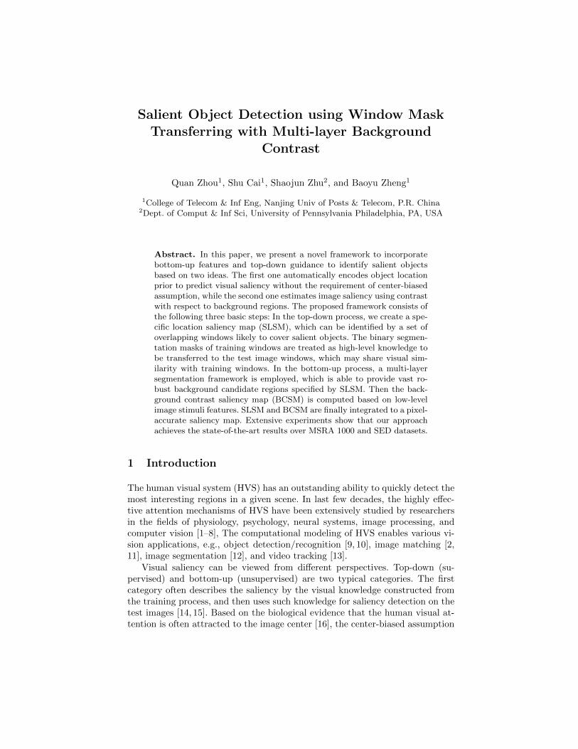
Fig. 1. Our approach consists of two components: (1) Top-down process. Given thetraining data consists of images with annotated binary segmentation masks, we firstemploy the technique of [9] to detect windows likely to contain salient objects on alltraining images and testing images. Then the binary segmentation masks of trainingwindows are transferred to each detective windows in testing image with the mostsimilar appearance (window neighbours). The transferred segmentation masks are usedto derive the specific location saliency map (SLSM); (2) Bottom-up process. Using theover-segmentation technique of [25], an input testing image is first partitioned to multi-layer segmentation in a coarse to fine manner. Given the SLSM as prior map, a set ofrobust background regions are abstracted, and then the color-based contrast saliencymaps are created for each layer of segmentation. These saliency maps are combinedto form our background contrast saliency map (BCSM). SLSM and BCSM are finallyintegrated to a pixel-accurate saliency map. (Best viewed in color)

is often employed as the location prior for estimating visual saliency in top-downmodels [17, 15].

While the salient regions are mostly located in the image center, the inversemight not necessarily be true [18, 19]. Not all image center regions tend to bemore salient. The salient object might be located far away from image center,even on the image boundary. Furthermore, a center-biased assumption alwayssupposes that there is only one salient object within each image, yet it oftenfails when nature image contains two or more salient objects [19]. Thus, todetect salient regions without center-biased constrains, some semantic knowledge(e.g., face and pedestrian) are integrated in a top-down process, which is mostlybased on object detectors [14, 20, 17]. The integration, however, acts rather moregeneral on object category level than at the saliency-map level.

On the other hand, the bottom-up models are mainly motivated from the con-trast formulation. For example, Itti et al. [1, 21] proposed a set of pre-attentivefeatures including local center-surround intensity, color and direction contrasts.These contrasts were then integrated to compute image saliency through thewinner-take-all competition. Cheng et al. [22] and Achanta et al. [23] utilizethe global contrast with respect to the entire scene to estimate visual saliency.Recently, Borji and Itti [24] combine local and global patch rarities as contrastto measure saliency for eye-fixation task. We argue that the contrast based onbackground regions also plays an important role in such processes.

Title Suppressed Due to Excessive Length 3

In this paper, we propose a novel method to integrate bottom-up, lower-level features and top-down, higher-level priors for salient object detection. Ourapproach is fully automatic and requires no center-biased assumption. The keyidea of our top-down process is inspired by [26], where the binary segmentationmasks are treated as prior information to be transferred from the supervisedtraining image set to the testing image set. Then, the transferred segmentationmasks are used to derive specific location prior of salient object in the test image.

Figure 1 illustrates the overview of our method. The basic intuition is thatthe windows with similar visual appearance often share similar binary segmen-tation masks. Since these transferred windows exhibit less visual variability thanthe whole scenes and are often centered on the salient regions, they are muchsuitable for location transfer with better support regions. As a result, we utilizethe method of [9] to extract candidate windows that are likely to contain salientobjects, and then transfer training window segmentation masks that share vi-sual similarity to windows in the test image. Afterwards, the bottom-up saliencymap is computed based on low-level image stimuli features. In nature images,although the salient regions and backgrounds may also tend to be perceptuallyheterogeneous, the appearance cues (e.g., color and texture) of the salient objectregion are still quite different from the backgrounds. Therefore, different from theprevious methods that mainly utilize the local central-surround contrast [1, 15,24] and global contrast [23, 22, 27] to encode saliency, our framework estimatesvisual saliency using the appearance-based contrast with respect to the back-ground candidate regions. In order to automatically abstract robust backgroundregions, we employ the multi-layer segmentation framework, which is able toprovide large amount of background candidates within different sizes and scales.

The contributions of our approach are three-fold:(1) In the top-down process, it proposes a specific location prior for salient

object detection. Through window mask transferring, our method is able toprovide more accurate location prior to detect salient regions, which results inmore accurate and reliable saliency maps than the models using center-biasedassumptions, such as [16] and [17];

(2) In the bottom-up process, unlike the previous approaches that utilize thelocal and global contrast to predict visual saliency, we attempt to estimate visualsaliency using the contrast with respect to the background regions;

(3) Compared with most competitive models [1, 22, 14, 28, 17, 23, 18, 29, 27,30, 31], our method achieves the state-of-the-art results over MSRA 1000 andSED datasets.

2 Related Work

In this section, we focus on reviewing the existing work for salient object de-tection, which can be roughly classified into two categories: bottom-up and top-down models.

The bottom-up approaches select the unique or rare subsets in an image asthe salient regions [1, 32, 28, 33]. As a pioneer work, Itti et al. [1] introduced


a biologically inspired saliency model based on the center-surround operation.Graph-based models [29, 34] are suggested to predict saliency following the prin-ciple of Markov random walk theory. Some researchers attempt to detect irregu-larities as visual saliency in the frequency domain [27, 23, 35]. Bruce and Tsotsos[36] established a bottom-up model following the principle of maximizing in-formation sampled from a scene. Sparsity models [37, 17] are also employed toencode saliency, where the salient regions are identified as sparse noises whenrecovering the low-rank matrix.

Despite the success of these models, they are difficult to generalize to real-word scenes. Instead, some researchers attempt to incorporate the top-down pri-ors for salient object detection [15, 10, 20]. Li et al. [38] and Ma et al. [39] formu-late the top-down factors as high level semantic cues (e.g., faces and pedestrian).Alternatively, Navalpakkam and Itti [40] modeled the top-down gain optimiza-tion as maximizing the signal-to-noise ratio (SNR). Liu et al. [15] proposed toadopt a conditional random field (CRF) model for predicting visual saliency.Bayesian modeling is also used for combining sensory evidence with prior con-strains. In these models, the prior knowledge (such as scene context [14] or gistdescriptors [41]) and sensory evidence (such as target features [42]), are proba-bilistically combined according to Bayesian rule. Different from these methods,our method employs the specific location prior as top-down knowledge by trans-ferring window segmentation masks.

3 Our Approach

In this section, we elaborate on the details of our method. We first introducehow to obtain the specific location saliency map (SLSM) by transferring win-dow masks. Given the multi-layer segmentations and SLSM on hand, we selecta series of background regions that are used to compute background contrastsaliency map (BCSM). Finally, two maps are incorporated to generate pixel-wised saliency.

3.1 Specific Location Saliency Map (SLSM)

Finding Similar Windows. In order to utilize the prior knowledge of anno-tated binary segmentation mask in the training set, we first detect windowslikely to contain an object using the ”objectness” technique of [9]. It tends to re-turn more windows covering an object with a well-defined boundary, rather thanamorphous background elements. In our experiments, sampling only N windowsper image (e.g., N = 100) seems enough to cover most salient objects. Puttingall the training windows together, we obtain the training window set {Wt}. Thisleads to retrieving much better neighborhood windows with similar appearance,whose segmentation masks are more suitable to transfer for test image. Givena new test image I as illustrated in Figure 2(a), the N number of “objectness”windows are also extracted using [9] as well as for the training images. Figure


(a) Test image I (b) Windows Wk of I (c) Windows neighbors in training windows {Wt} and corresponding binary map {Sk}

(d) Window soft masks (Mk) (e) SLSM

red

green

blue

Fig. 2. An example of the full pipeline for producing SLSM. Given a test image I in (a),three top windows (denoted as red, green and blue rectangles) are highlighted out of Nwindows, as shown in (b). The window neighbors are displayed in (c). It is shown thatgreen window is tightly centered on an object and gets very good neighbors, while forred and blue windows, the neighbors are good matches for transferring segmentationmask, even though these windows do not cover the ”horse” perfectly. This results inan accurate transfer mask for each window of I, as illustrated in (d). On the rightmostcolumn of (e), we integrate the soft mask Mk from all windows into a soft mask for thewhole scene, which is used to derive the SLSM. Note blue color denotes low saliency,while red color represents high saliency (Best viewed in color)

2(b) shows top three ”objectness” windows in the test image I, and it is ob-served that many detective windows are centered on the salient object “horse”.For one specific test window Wk, k = {1, 2, · · · ,N}, we compute GIST feature[43] inside Wk to describe its appearance, and compare GIST descriptors withthe `2-norm distance to all training windows {Wt} to find window neighbors.Thus, the set {Sjk}, j = {1, 2, · · · ,M} containing the segmentation masks of thetopM training windows most similar to Wk is used for transferring. Figure 2(c)illustrates that the nearest neighbor windows accurately depict similar animalsin similar poses, resulting in well-matched binary segmentation masks.Segmentation Transfer. Let ST (x, y) be the SLSM, which defines the prob-ability of pixel at location (x, y) to be salient. We construct ST (x, y) for eachpixel from the segmentation masks transferred from all windows containing it.

1) Soft masks for windows. For the kth test window Wk, we have a set ofbinary segmentation masks {Sjk} of neighbor windows from the training set. Herewe compute a soft segmentation mask Mk for each Wk as the pixel-wise mean ofthe masks in {Sjk}. To this end, all masks in {Sjk} are resized to the resolution

of Wk. Let {Sj′

k } be the resized masks, then the soft mask Mk for window Wk

is defined as:

Mk =1

M

M∑j′=1

Sj′

k (1)

In this aligned space, a pixel value in Mk corresponds to the probability for it

to be a salient object in {Sj′

k }. Figure 2(d) shows the corresponding Mk for thedetected windows. Note the resolution of each soft window mask Mk is the sameas the one of detected window in Figure 2(b).

2) Soft mask for the test image. After obtaining soft masks Mk, we integrateMk for all windows into a single soft segmentation mask M(x, y) for the testimage I. For each window Wk, we place its soft mask Mk at the image location


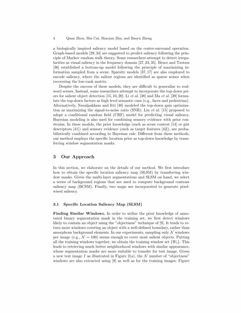
Fig. 3. Illustration of SLSM. The first and third rows are the example images formMSRA 1000 and SED dataset, respectively. The second and fourth rows are the corre-sponding SLSM, where blue color denotes low saliency, while red color represents highsaliency. (Best viewed in color)

(x, y) defined by Wk. The soft mask M(x, y) of the test image is the pixel-wisemean of all N placed masks Mk(x, y):

M(x, y) =1

N

N∑k=1

Mk(x, y) (2)

A pixel value in M(x, y) is the probability for it to be salient, according to alltransferred segmentations (as illustrated in Figure 2(d)). Therefore, we definethe SLSM ST (x, y) as

ST (x, y) = M(x, y) (3)

Due to the integration of all soft segmentation masks Mk(x, y) from the indi-vidual windows, our approach achieves even more robust results. The key step ofour approach is that we extract many windows (e.g., 100 per image) overlappingsalient object. One effect is that a certain window might not have good neighborsin the training set, leading to transferring an inaccurate or even completely in-correct mask Mk(x, y). However, other overlapping windows will probably havegood neighbors, diminishing the effect of the inaccurate Mk(x, y) in the integra-tion step. Another effect may happen when the transferred windows may notcover a salient object, (e.g., detecting a patch on the backgrounds, as the bluewindow shown in Figure 1). This does not pose a problem to our approach, asthe training images are decomposed in the same type of windows [9]. Therefore,a background window will probably also has similar appearance neighbors onbackgrounds in the training images, resulting in correctly transferring a back-ground binary segmentation mask. As a result, our approach is fully symmetricover salient and background windows. Figure 3 exhibits some SLSMs of natureimages over MSRA 1000 and SED datasets.


Fig. 4. Image representation by multi-layer segmentation. The upper panel shows theexamples from MSRA dataset, while the bottom panel illustrates the examples fromSED dataset. From left to right are the original images and their over-segmentationresults in a coarse to fine manner. Different segments are separated by white boundaries.

3.2 Background Contrast Saliency Map (BCSM)

No matter where the salient object locates, it often exhibits quite different ap-pearance cues (e.g., color and texture) within the entire scene. We thus buildour background contrast saliency map (BCSM) guided by the global color-basedcontrast measurement [22]. Instead of computing saliency based on an entireimage, here we calculate the contrast based on background candidates.Multi-layer Segmentation. In order to make full use of background candidateregions, we employ the multi-layer segmentation framework.

Traditionally, an image is typically represented by a two-dimensional arrayof RGB pixels. With no prior knowledge of how to group these pixels, we cancompute only local cues, such as pixel colors, intensities or responses to convo-lution with bank of filters [44, 45]. Alternatively, we use the SLIC algorithm [25]to implement over-segmentation, since it performs more efficiently. In practice,we partition test image I into J layers of segmentations. There are two parame-ters to be tuned for this segmentation algorithm, namely (rgnSize, regularizer),which denote the number of segments used for over-segmentation and the trade-off appearance for spatial regularity, respectively. As shown in Figure 4, the


advantages of using this technique are that it can often group the homogeneousregions with similar appearance and preserve the true boundary of objects.

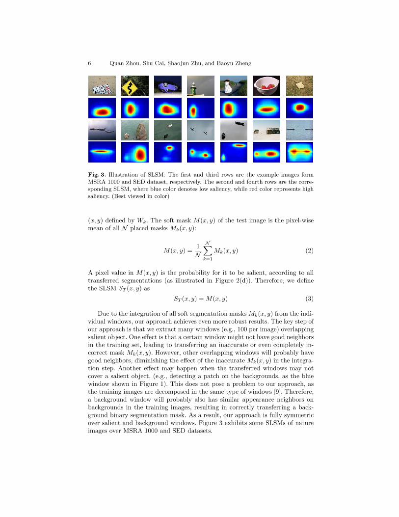
Computing BCSM. Denote SB(x, y) as the BCSM to convey a sense of thedissimilarity of a pixel based on its local feature with respect to backgrounds, sothat SB(x, y) also gives the probability of pixel at location (x, y) to be salient.We construct SB(x, y) for each pixel from the multi-layer segmentation via allsegments containing it.

1) Color contrast saliency for each layer segmentation. Let rji be ith specificsegment in jth layer of segmentation. According to the SLSM, we select thesegments with low saliency value to be background candidates, which are readyto compute the color-based contrast saliency. Let Bj = {Bj1, B

j2, · · · , B

jM} be

selected background candidate regions in jth layer segmentation. To measurehow distinct the salient region is with respect to Bjm ∈ Bj , we can measure thedistance between rji and Bjm using various visual cues such as intensity, color,and texture/texton. In this paper, we use the inverse cosine distance betweenhistograms of HSV space to compute the color-based contrast:

Cji,m(H(rji ),H(Bjm)) = 1− H(rji )TH(Bjm)

||H(rji )|| · ||H(Bjm)||(4)

where H(·) is the binned histogram calculated from all color channels of onesegment, and || · || denotes the `2 norm. We use histograms because they are arobust global description of appearance. They are insensitive to small changes insize, shape, and viewpoint. From Equation (4), it is observed that the contrastbetween rji and Bjm is very low when they look similar, otherwise not. For the

given segment rji , its color contrast saliency SB(rji ) is computed as the mean of

L smallest contrasts in {Cji,m(·, ·)},m = 1, 2, · · · ,M

SB(rji ) =1

L

L∑m=1

Cji,m(·, ·) (5)

As will be seen, when rji is truly a salient region, the L smallest contrasts alwaysget large value with respect to the background regions, resulting in high saliencyfor SB(rji ). The saliency map SB(rji ) is normalized to a fixed range [0, 255], and

SB(rji ) is assigned to each image pixel belonging to rji with the saliency value

as SjB(x, y).

2) BCSM for testing image. We now incorporate the SjB(x, y) for all segmen-tation layers into a single saliency map for the test image I. Then the BCSMSB(x, y) is defined as:

SB(x, y) =1

J

J∑j=1

SjB(x, y) (6)

SB(x, y) is also normalized to a fixed range [0, 255].


3.3 Combined Saliency

We integrate SLSM and BCSM to produce our final saliency map S(x, y) witha linearly combination model

S(x, y) = η · ST (x, y) + (1− η) · SB(x, y) (7)

where η is the harmonic parameter to balance the top-down SLSM and bottom-up BCSM. Then S(x, y) is normalized to a fixed range [0, 255].

4 Experimental Results

To validate our proposed method, we carried out several experiments on twobenchmark datasets using the Precision-Recall curve and F-measure describedbelow. The main reason behind employing several datasets is that current datasetshave different image and feature statistics, stimulus varieties, and center-biases.Hence, it is necessary to employ several datasets as models leverage differentfeatures that their distribution varies across datasets.

Datasets. We test our proposed model on two datasets: (1) Microsoft ResearchAsian (MSRA) 1000 dataset [23] is the most widely used and as baseline bench-mark for evaluating salient object detection models. It contains 1000 imageswith resolution of approximate 400 × 300 or 300 × 400 pixels, which only haveone salient object per image and provides accurate object-contour-based groundtruth. (2) The SED [19] dataset is a smaller dataset only containing 100 imageswith resolution ranged from 300×196 to 225×300 pixels. The reason to employthis dataset lies in that it is not center-biased and there are two salient objectsin each image. Therefore, this dataset is more challenging for the task of salientobject detection.

Baselines. To show the advantages of our method, we selected 12 state-of-the-art models as baselines for comparison, which are spectral residual saliency (SR[27]), spatiotemporal cues (LC [31]), visual attention measure (IT [1]), graph-based saliency (GB [29]), frequency-tuned saliency (FT [23]), salient region de-tection (AC [30]), context-aware saliency (CA [14]), global-contrast saliency (HCand RC [22]), saliency filter (SF [28]), low rank matrix recovery (LR [17]), andgeodesic saliency (SP [18]). In practice, we implemented all the 12 state-of-the-art models using a Dual Core 2.6 GHz machine with 4GB memory over twodatasets to generate saliency maps.

Evaluation Metrics. In order to quantitatively evaluate the effectiveness of ourmethod, we conducted experiments based on the following widely used criteria.The precision-recall curve (PRC) is used to evaluate the similarity between thepredicted saliency maps and the ground truth. Precision corresponds to the per-centage of salient pixels correctly assigned, while recall corresponds to the frac-tion of detected salient pixels in relation to the ground truth number of salientpixels. Another criterion to evaluate the overall performance is the F-measure[23, 22], which is used to weight harmonic mean measurement of precision and


0 0.1 0.2 0.3 0.4 0.5 0.6 0.7 0.8 0.9 10.1

0.2

0.3

0.4

0.5

0.6

0.7

0.8

0.9

1

ITGBCAACRCHCOurs

Recall

Prec

isio

n

Recall

Prec

isio

n

0 0.1 0.2 0.3 0.4 0.5 0.6 0.7 0.8 0.9 10.1

0.2

0.3

0.4

0.5

0.6

0.7

0.8

0.9

1

FTLCSRSPSFLROurs

AC CA FT GB IT LC RC HC SR LR SP SF Ours0

0.1

0.2

0.3

0.4

0.5

0.6

0.7

0.8

0.9

1

RecallF-measurePrecision

Fig. 5. Quantitative comparison for all algorithms with naive thresholding of saliencymaps using 1000 publicly available benchmark images. Left and middle: PRC of ourmethod compared with CA [14], AC [30], IT [1], LC [31], SR [27], GB [29], SF [28], LR[17], FT [23], SP [18], HC and RC [22]. Right: Average precision, recall and F-measurewith adaptive-thresholding segmentation. Our method shows high precision, recall, andFβ values on the MSRA 1000 dataset. (Best viewed in color)

recall. The F-measure is defined as

Fβ =(1 + β2)× Precision×Recallβ2 × Precision+Recall

(8)

where β2 = 0.3 following [23, 22].Implemented Details. In order to make our approach work well, it is im-portant to establish a large and diverse training set, which is able to providesufficient appearance statistics to distinguish salient regions and background. Inour implementation, we employ the full PASCAL VOC 2006 [46] as our train-ing dataset, since it includes more than 5000 images with accurate annotatedobject-contour-based ground truth.

The parameter settings are: N = 100 for sampling windows per image,M =100 for window neighbors for one sampling window, J = 5 for segmentationlayers in a coarse to fine manner, L = 5 for computing color contrast saliencyinvolved in Equation (5), (rgnSize, regularizer) are initialized as {25, 10}, andrgnSize is updated as {25, 50, 100, 200, 400} with fixed regularizer, η = 0.6 tobalance SLSM and BCSM for producing final saliency map.

We follow two widely used methodologies [23, 17] to implement our exper-iments. In the first implementation, we adopt the scheme that segments im-age according to the saliency values with a fixed threshold. Given a thresholdT ∈ [0, 255], the regions whose saliency values are higher than threshold aremarked as a salient object. The segmented image is then compared with theground truth to obtain the precision and recall. We draw the PRC using a seriesof precision-recall pairs by varying T from 0 to 255.

In the second implementation, the test image is segmented by an adaptivethreshold method [17]. Given the over-segmented image, an average saliency iscalculated for each segment. Then an overall mean saliency value over the entireimage is obtained as well. If the saliency in this segment is larger than twice ofthe overall mean saliency value, the segment is marked as foreground. Precision


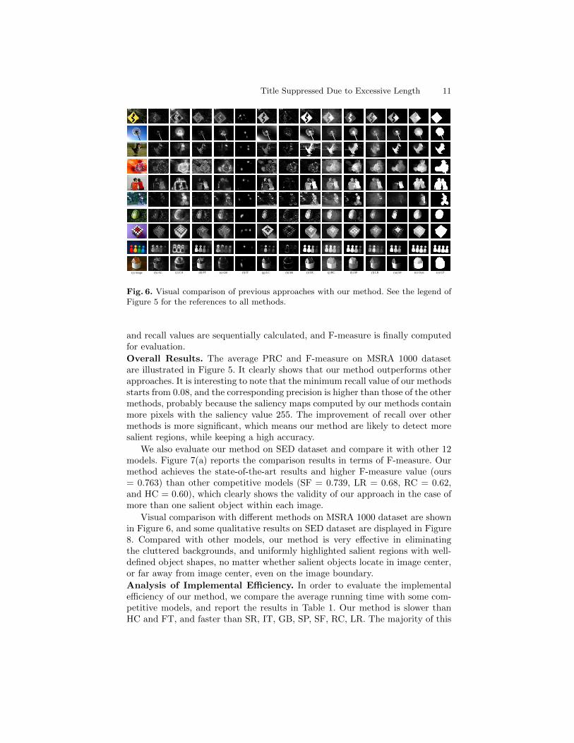
(a) image (b) AC (c) CA (f) IT(e) GB(d) FT (g) LC (i) HC(h) SR (m) SF(j) RC (n) Ours (o) GT(k) SP (l) LR

Fig. 6. Visual comparison of previous approaches with our method. See the legend ofFigure 5 for the references to all methods.

and recall values are sequentially calculated, and F-measure is finally computedfor evaluation.

Overall Results. The average PRC and F-measure on MSRA 1000 datasetare illustrated in Figure 5. It clearly shows that our method outperforms otherapproaches. It is interesting to note that the minimum recall value of our methodsstarts from 0.08, and the corresponding precision is higher than those of the othermethods, probably because the saliency maps computed by our methods containmore pixels with the saliency value 255. The improvement of recall over othermethods is more significant, which means our method are likely to detect moresalient regions, while keeping a high accuracy.

We also evaluate our method on SED dataset and compare it with other 12models. Figure 7(a) reports the comparison results in terms of F-measure. Ourmethod achieves the state-of-the-art results and higher F-measure value (ours= 0.763) than other competitive models (SF = 0.739, LR = 0.68, RC = 0.62,and HC = 0.60), which clearly shows the validity of our approach in the case ofmore than one salient object within each image.

Visual comparison with different methods on MSRA 1000 dataset are shownin Figure 6, and some qualitative results on SED dataset are displayed in Figure8. Compared with other models, our method is very effective in eliminatingthe cluttered backgrounds, and uniformly highlighted salient regions with well-defined object shapes, no matter whether salient objects locate in image center,or far away from image center, even on the image boundary.

Analysis of Implemental Efficiency. In order to evaluate the implementalefficiency of our method, we compare the average running time with some com-petitive models, and report the results in Table 1. Our method is slower thanHC and FT, and faster than SR, IT, GB, SP, SF, RC, LR. The majority of this


Table 1. Average running time of different methods on MSRA 1000 dataset.

Method SR [27] IT [1] GB [29] FT [23] SP [18]

Time(s) 0.064 0.611 1.614 0.016 1.213

Code Matlab Matlab Matlab C++ Matlab

Method HC [22] RC [22] SF [28] LR [17] ours

Time(s) 0.019 0.253 0.153 1.748 0.759

Code C++ C++ C++ Matlab Matlab

AC SR FT LC SP GB IT CA HC RC LR SF Ours0

0.1

0.2

0.3

0.4

0.5

0.6

0.7

0.8

0 0.1 0.2 0.3 0.4 0.5 0.6 0.7 0.8 0.9 10.1

0.2

0.3

0.4

0.5

0.6

0.7

0.8

0.9

1

Ours(l=1)Ours(l=2)Ours(l=3)Ours(l=4)Ours(l=5)SLSM

0 0.1 0.2 0.3 0.4 0.5 0.6 0.7 0.8 0.9 10.2

0.3

0.4

0.5

0.6

0.7

0.8

0.9

1

Ours(l=1)Ours(l=2)Ours(l=3)Ours(l=4)Ours(l=5)SLSM

Recall

Prec

isio

n

Recall

Prec

isio

n

(b) (c)(a)

Fig. 7. Left: From left to right: (a) F-measure of the different saliency models to groundtruth on SED dataset. (b) and (c) The comparison of PRC by gradually increasing thelayers of segmentation on MSRA 1000 and SED dataset, respectively. In (b) and (c),the performance of individual SLSM is also included. (Best viewed in color)

Fig. 8. Some visual examples on SED dataset. The first, third and fifth columnsare original images, and the second, fourth and sixth columns are the correspondingsaliency maps. (Best viewed in color)

time is spent performing multi-layer segmentation, producing detected window,and computing window neighbours (about 80%), and only 20% account for theactual saliency computation.

Analysis of Parameter Setting and Individual Saliency Map. One factoraffecting the performance is the layers of over-segmentation. Figure 7(b) and (c)


exhibit the plot of PRC with different number of segmentation layers on theMSRA 1000 and SED datasets, respectively. It is observed that better perfor-mance can be achieved along with the increasement of segmentation layers, andno further improvement after 5 layer segmentations. This demonstrates that ourmethod performs robustly over a wide range of segmentation layers.

In order to evaluate the contributions of each individual saliency map, thePRC of SLSM is also included for comparison in Figure 7(b) and (c). The per-formance of SLSM is already better than most of the competitive models, whoseresults are shown in Figure 5. Using BCSM noticeably improves the perfor-mance for both two datasets, which indicates the importance of measuring visualsaliency using contrast with respect to background regions.

5 Conclusion and Future Work

In this paper, we propose a novel framework for salient object detection basedon two key ideas: (1) using specific location information as top-down prior bytransferring segmentation masks from windows in the training images that arevisually similar to windows in the test image; (2) using the contrast based onthe background candidates in bottom-up process makes our method more robustthan methods estimating contrast on the entire image. Compared with existingcompetitive models, the extensive experiments show that our approach achievesthe state-of-the-art results over MSRA 1000 and SED datasets. In the future,we would like to combine two saliency maps, SLSM and BCSM, with adaptiveweights using learning technique, as well as [47] does.

Acknowledgement. The authors would like to thank all the anonymous re-viewers valuable comments. We would like to thank Prof. Liang Zhou for hisvaluable comments to improve the readability of the whole paper. This workwas supported by NSFC 61201165, 61271240, 61401228, 61403350, PAPD andNY213067.

References

1. Itti, L., Koch, C., Niebur, E.: A model of saliency-based visual attention for rapidscene analysis. TPAMI 20 (1998) 1254–1259

2. Zhao, R., Ouyang, W., Wang, X.: Person re-identification by salience matching.In: ICCV. (2013) 73–80

3. Jiang, H., Wang, J., Yuan, Z., Wu, Y., Zheng, N., Li, S.: Salient object detection: Adiscriminative regional feature integration approach. In: CVPR. (2013) 2083–2090

4. Yan, Q., Xu, L., Shi, J., Jia, J.: Hierarchical saliency detection. In: CVPR. (2013)1155–1162

5. Borji, A., Tavakoli, H.R., Sihite, D.N., Itti, L.: Analysis of scores, datasets, andmodels in visual saliency prediction. In: CVPR. (2013) 921–928

6. Li, X., Lu, H., Zhang, L., Ruan, X., Yang, M.H.: Saliency detection via dense andsparse reconstruction, ICCV (2013)


7. Yang, C., Zhang, L., Lu, H., Ruan, X., Yang, M.H.: Saliency detection via graph-based manifold ranking. In: CVPR. (2013) 3166–3173

8. Marchesotti, L., Cifarelli, C., Csurka, G.: A framework for visual saliency detectionwith applications to image thumbnailing. In: ICCV. (2009) 2232–2239

9. Alexe, B., Deselaers, T., Ferrari, V.: What is an object? In: CVPR. (2010) 73–8010. Gao, D., Han, S., Vasconcelos, N.: Discriminant saliency, the detection of suspicious

coincidences, and applications to visual recognition. TPAMI 31 (2009) 989–100511. Toshev, A., Shi, J., Daniilidis, K.: Image matching via saliency region correspon-

dences. In: CVPR. (2007) 1–812. Jung, C., Kim, C.: A unified spectral-domain approach for saliency detection and

its application to automatic object segmentation. TIP 21 (2012) 1272–128313. Mahadevan, V., Vasconcelos, N.: Saliency-based discriminant tracking. In: CVPR.

(2009) 1007–101314. Goferman, S., Zelnik-Manor, L., Tal, A.: Context-aware saliency detection. In:

CVPR. (2010) 2376–238315. Liu, T., Yuan, Z., Sun, J., Wang, J., Zheng, N., Tang, X., Shum, H.: Learning to

detect a salient object. TPAMI 33 (2011) 353–36716. Tatler, B.: The central fixation bias in scene viewing: Selecting an optimal viewing

position independently of motor biases and image feature distributions. Journal ofVision 7 (2007) 1–17

17. Shen, X., Wu, Y.: A unified approach to salient object detection via low rankmatrix recovery. In: CVPR. (2012) 853–860

18. Wei, Y., Wen, F., Zhu, W., Sun, J.: Geodesic saliency using background priors.In: ECCV. (2012)

19. Borji, A., Sihite, D.N., Itti, L.: Salient object detection: A benchmark. In: ECCV.(2012) 414–429

20. Judd, T., Ehinger, K., Durand, F., Torralba, A.: Learning to predict where humanslook. In: ICCV. (2009) 2106–2113

21. Itti, L., Koch, C.: A saliency-based search mechanism for overt and covert shiftsof visual attention. Vision research 40 (2000) 1489–1506

22. Cheng, M., Zhang, G., Mitra, N., Huang, X., Hu, S.: Global contrast based salientregion detection. In: CVPR. (2011) 409–416

23. Achanta, R., Hemami, S., Estrada, F., Susstrunk, S.: Frequency-tuned salientregion detection. In: CVPR. (2009) 1597–1604

24. Borji, A., Itti, L.: Exploiting local and global patch rarities for saliency detection.In: CVPR. (2012) 478–485

25. Achanta, R., Shaji, A., Smith, K., Lucchi, A., Fua, P., Susstrunk, S.: Slic super-pixels. EPEL, Tech. Rep 149300 (2010)

26. Kuettel, D., Ferrari, V.: Figure-ground segmentation by transferring windowmasks. In: CVPR. (2012) 558–565

27. Hou, X., Zhang, L.: Saliency detection: A spectral residual approach. In: CVPR.(2007) 1–8

28. Perazzi, F., Krahenbuhl, P., Pritch, Y., Hornung, A.: Saliency filters: Contrastbased filtering for salient region detection. In: CVPR. (2012) 733–740

29. J., H., C., K., P., P.: Graph-based visual saliency. In: NIPS. (2006) 545–55230. Achanta, R., Estrada, F., Wils, P., Susstrunk, S.: Salient region detection and

segmentation. Computer Vision Systems (2008) 66–7531. Zhai, Y., Shah, M.: Visual attention detection in video sequences using spatiotem-

poral cues. In: ACMMM. (2006) 815–82432. Parkhurst, D., Law, K., Niebur, E.: Modeling the role of salience in the allocation

of overt visual attention. Vision research 42 (2002) 107–124


33. Wang, W., Wang, Y., Huang, Q., Gao, W.: Measuring visual saliency by siteentropy rate. In: CVPR. (2010) 2368–2375

34. Gopalakrishnan, V., Hu, Y., Rajan, D.: Random walks on graphs for salient objectdetection in images. TIP 19 (2010) 3232–3242

35. Guo, C., Ma, Q., Zhang, L.: Spatio-temporal saliency detection using phase spec-trum of quaternion fourier transform. In: CVPR. (2008) 1–8

36. Bruce, N., Tsotsos, J.: Saliency based on information maximization. In: NIPS.(2006) 155–162

37. Lang, C., Liu, G., Yu, J., Yan, S.: Saliency detection by multi-task sparsity pursuit.TIP 21 (2012) 1327–1338

38. Li, J., Tian, Y., Huang, T., Gao, W.: Probabilistic multi-task learning for visualsaliency estimation in video. IJCV 90 (2010) 150–165

39. Ma, Y.F., Hua, X.S., Lu, L., Zhang, H.J.: A generic framework of user attentionmodel and its application in video summarization. TMM 7 (2005) 907–919

40. Navalpakkam, V., Itti, L.: Search goal tunes visual features optimally. Neuron 53(2007) 605–617

41. Torralba, A., Oliva, A., Castelhano, M., Henderson, J.: Contextual guidance of eyemovements and attention in real-world scenes: the role of global features in objectsearch. Psychological review 113 (2006) 766–786

42. Zhang, L., Tong, M., Marks, T., Shan, H., Cottrell, G.: Sun: A bayesian frameworkfor saliency using natural statistics. Journal of Vision 8 (2008) 1–20

43. Oliva, A., Torralba, A.: Modeling the shape of the scene: A holistic representationof the spatial envelope. IJCV 42 (2001) 145–175

44. Comaniciu, D., Meer, P.: Mean shift: A robust approach toward feature spaceanalysis. TPAMI 24 (2002) 603–619

45. Shi, J., Malik, J.: Normalized cuts and image segmentation. TPAMI 22 (2000)888–905

46. Everingham, M., Zisserman, A., Williams, C.K.I., Van Gool, L.: The PASCALVisual Object Classes Challenge 2006 (VOC2006) Results. (http://www.pascal-network.org/challenges/VOC/voc2006/results.pdf)

47. Itti, L., Koch, C.: Feature combination strategies for saliency-based visual attentionsystems. Journal of Electronic Imaging 10 (2001) 161–169

salient object detection using window mask...

Documents