salience and taxation with imperfect competition

Salience and Taxation with Imperfect Competition

Kory Kroft, Jean-William P. Laliberté, René Leal-Vizcaíno, and Matthew J. Notowidigdo∗

December 2020

Abstract

This paper studies commodity taxation in a model featuring heterogeneous consumers, imper-fect competition, and tax salience. We derive new formulas for the incidence and marginal excessburden of commodity taxation, and we find that tax salience and market structure interact whenconsidering tax incidence and the marginal excess burden. We estimate the necessary inputs to theformulas by combining Nielsen Retail Scanner data from grocery stores in the US with detailedsales tax data. We calibrate our new formulas and conclude that essentially all of the incidence ofsales taxes falls on consumers, and the marginal excess burden of taxation is larger than estimatesbased on standard formulas that ignore imperfect competition and tax salience.

∗Kroft: University of Toronto and NBER, [email protected]; Laliberté: University of Calgary, [email protected]; Leal-Vizcaíno: Bank of Mexico, [email protected]; Notowidigdo: University ofChicago Booth School of Business and NBER; [email protected]. We thank Simon Anderson, Raj Chetty, JulieCullen, Amy Finkelstein, Xavier Gabaix, Nathan Hendren, Louis Kaplow, Henrik Kleven, Nicholas Li, Jesse Shapiro, RobPorter, Aviv Nevo, Stephen Coate, and numerous seminar participants for helpful comments. We thank Eileen Driscoll,Robert French, Adam Miettinen, Boriana Miloucheva, Pinchuan Ong, Shahar Rotberg, Marc-Antoine Schmidt, StephenTino, Jessica Wagner, Ting Wang, Haiyue Yu, and Ruizhi Zhu for extremely valuable research assistance. We grate-fully acknowledge funding from the Social Sciences and Humanities Research Council (SSHRC). Any opinion, findings,and conclusions or recommendations expressed in this material are those of the authors(s) and do not necessarily reflectthe views of the SSHRC. This research is based in part on data from The Nielsen Company (US), LLC and market-ing databases provided through the Nielsen Datasets at the Kilts Center for Marketing Data Center at The University ofChicago Booth School of Business. The conclusions drawn from the Nielsen data are those of the researchers and do notreflect the views of Nielsen. Nielsen is not responsible for, had no role in, and was not involved in analyzing and preparingthe results reported herein.

1 Introduction

Standard welfare analysis of commodity taxation typically makes two key assumptions: (1) the prod-

uct market is perfectly competitive and (2) consumers respond to taxes in the same way they respond

to price changes. Several papers in public economics have relaxed the first assumption (see Auerbach

and Hines 2002 for a review of this literature), but these papers have maintained the second as-

sumption that taxes are fully salient. More recently, researchers have relaxed the second assumption,

developing new theoretical and empirical tools to analyze the welfare effects of taxes when taxes are

less salient than prices, but have maintained the assumption of perfect competition (Chetty, Looney,

and Kroft 2009; Taubinsky and Rees-Jones 2018; Farhi and Gabaix 2020; Morrison and Taubinsky

2020). If markets are characterized by imperfect competition and consumers misperceive taxes, how-

ever, neither of these approaches is likely to provide a fully accurate characterization of the welfare

effects of commodity taxes.

In this paper, we derive new formulas for the incidence and marginal excess burden of commodity

taxes (both unit taxes and ad valorem taxes) in a model featuring imperfect competition and tax

salience with heterogeneous consumers. Using these formulas, we show how tax salience and market

structure interact when considering tax incidence and the marginal excess burden.

For incidence, we show that greater attention to taxes can increase the incidence on consumers

under imperfect competition in contrast to the standard model of perfect competition which predicts

the opposite pattern. Thus, the standard intuition of how tax salience affects the incidence of taxation

in perfectly competitive markets does not always carry over to imperfect competition. We also derive

new results about how heterogeneity in consumer inattention to taxes affects incidence both under

perfect competition and imperfect competition.1 We show that consumer heterogeneity affects pass-

through and incidence under all market structures including perfect competition. With imperfect

competition, there is an additional effect of heterogeneity on pass-through. Intuitively, when the

1While Taubinsky and Rees-Jones (2018) study how consumer heterogeneity affects the efficiency cost of taxationunder perfect competition, they do not consider incidence.

1

consumer response to taxes is heterogeneous, this effectively changes the slope of the inverse demand

curve facing the firm and firms take this into account when choosing prices. Of particular relevance

for firms with market power is how inattention correlates with the price elasticity of demand. We show

that firms bear less of the burden of taxes when elastic consumers are more inattentive to taxes. Thus,

the covariance between consumer inattention and price elasticity is important for incidence analysis.

Turning to welfare, we find that tax salience and market structure directly interact in the tax for-

mula characterizing the marginal excess burden of taxation. In particular, while the expression for the

marginal excess burden includes the additive effects of imperfect competition (via the markup) and

tax salience (via the inattention parameter), it also includes the output response to the tax which in

turn depends on the degree of inattention to the tax and the output response to prices. While salience

has a second-order effect on excess burden under perfect competition when there are no pre-existing

taxes (see Chetty, Looney and Kroft 2009), we show that it has a first-order effect under imperfect

competition and scales linearly with the markup. This is important since it highlights that, at least in

some circumstances, “behavioral biases” may have a second-order effect on the welfare cost of taxa-

tion in competitive markets but a first-order effect on this welfare cost when firms have market power.

Moreover, holding fixed market structure, we find that greater attention to taxes (lower “frictions”)

magnifies the distortionary effect of taxation under imperfect competition. We also find, similar to

Taubinsky and Rees-Jones (2018) and Farhi and Gabaix (2020), that heterogeneous inattention to

taxes induces misallocation, and we generalize these results by showing that this misallocation does

not directly interact with market structure. Specifically, we find that greater dispersion in inattention

increases the welfare cost of taxes in similar ways under perfect and imperfect competition.

After presenting our theoretical results, we provide new estimates of the necessary inputs to our

tax formulas using Nielsen Retail Scanner data covering grocery stores selling consumer goods in

the U.S. combined with county-level and state-level sales tax data. We estimate the effect of taxes

on consumer prices and quantity demanded using a regression model that leverages variation in sales

taxes within states and counties over time, and another regression model that focuses on differences

2

between “border pair” counties located on opposite sides of a state border (Holmes 1998; Dube,

Lester and Reich 2010). We also estimate the price elasticity of demand based on an instrumental

variable strategy which exploits the “uniform pricing” across stores within retail chains (DellaVigna

and Gentzkow 2019). Our estimates indicate nearly-complete pass-through of taxes onto consumer

prices, and a tax elasticity of demand that is smaller in magnitude than the price elasticity of demand.

We combine these estimates to provide a new estimate of tax salience, which is fairly similar to other

estimates reported in the literature.

Lastly, we calibrate our new tax formulas using these empirical estimates. A novel feature of

our approach is the use of the pass-through formula and the generalized Lerner index to calibrate the

average markup, which enters in the marginal excess burden formula. We then consider two types of

calibration exercises. First, we quantify the discrepancy if one “naively” computed the welfare cost

of taxation using the standard Harberger formula that ignores salience effects and assumes perfect

competition. Our results show that the standard Harberger formula (Harberger 1964) understates the

marginal excess burden of taxes, which contrasts with Chetty, Looney and Kroft (2009) who show

that when consumers underreact to taxes, the standard Harberger formula overstates the true marginal

excess burden of taxes. Intuitively, this is because there is a pre-existing distortion coming from

firms’ market power under imperfect competition. While the markup scales one-for-one in the excess

burden formula, the mean and variance of the tax salience parameter scale with the tax rate, just as in

the case of perfect competition. Second, we calibrate the excess burden of taxation in counterfactual

scenarios that increase the salience of sales taxes and change the market structure taking into account

the endogeneity of the output response to the tax and pass-through with respect to tax salience and

market structure. This counterfactual analysis is more appropriate if one wants to compare the welfare

consequences of taxation under different assumptions on the degree of market power and degree of

inattention to taxes. Our analysis of these scenarios reveal various interactions between tax salience

and imperfect competition in determining the pass-through of taxes into consumer prices, the effect

of taxes on quantity demanded, and ultimately the incidence and marginal excess burden.

3

Our paper is related to several streams of research. First, our paper builds on and contributes

to the literature on taxation and imperfect competition (see, e.g., Seade 1987; Stern 1987; Delipalla

and Keen 1992; Anderson, de Palma, and Kreider 2001a; Anderson, de Palma and Kreider 2001b;

Auerbach and Hines 2001; Weyl and Fabinger 2013; Hackner and Herzing 2016; Adachi and Fabinger

2019; Miravete, Seim, and Thurk 2018). Our paper innovates in several ways. First, we consider

a general model of imperfect competition and do not impose a functional form for preferences or

technology, similar to Weyl and Fabinger (2013).2 Second, we permit consumers to underreact to

taxes and allow for heterogeneity in the degree of underreaction. Third, we derive our new formulas

for both ad valorem and unit taxes (allowing for tax salience) and compare these formulas, which

is important since existing theoretical work finds that these taxes are not equivalent under imperfect

competition (Delipalla and Keen 1992). Lastly, we provide an empirical application that allows us to

calibrate our new formulas, which contributes to the literature studying sales taxes empirically (see,

e.g., Besley and Rosen 1999; Einav et al. 2014; Baker, Johnson, and Kueng 2018).

We also contribute to the literature in behavioral public economics (Liebman and Zeckhauser

2004; Chetty, Looney and Kroft 2009; Bordalo, Gennaioli, and Shleifer 2013; Goldin and Hominoff

2013; Koszegi and Szeidl 2013; Allcott and Taubinsky 2015; Caplin and Dean 2015; Taubinsky and

Rees-Jones 2018; Allcott, Lockwood, and Taubinsky 2018; Bradley and Feldman 2019; Farhi and

Gabaix 202; Morrison and Taubinsky 2020). Most of the papers in this literature assume perfect

competition. Bradley and Feldman (2019), which examines tax incidence in a monopoly setting with

inattentive consumers, is an important exception. Relative to this paper, we allow for heterogeneity

in tax salience across consumers, allow for more general forms of imperfect competition, and move

beyond incidence to also study the efficiency cost of taxation. The joint consideration of incidence

and efficiency analysis is important for our calibration approach, which combines both tax formulas

to identify the markup which appears in the marginal excess burden formula.

The remainder of the paper is organized as follows: Section 2 begins with a model of perfect

2Weyl and Fabinger (2013) only consider tax incidence. They do not consider the efficiency costs of taxation.

4

competition and considers the welfare effects of a unit tax. Section 3 extends the results to monopoly

and the general model of imperfect competition. Section 4 derives analogous formulas for the case

of an ad valorem tax and compares the incidence and efficiency costs of ad valorem and unit taxes.

Section 5 discusses the data and the empirical results. Section 6 presents the calibration results.

Section 7 concludes.

2 Perfect Competition

We are interested in characterizing the incidence and marginal excess burden effects of commodity

taxation allowing for salience effects. Following Weyl and Fabinger (2013), we define the incidence

of a unit tax t as I=dCS/dtdPS/dt

and the marginal excess burden of the tax as dWdt

= dCSdt

+ dPSdt

+ dRdt

where

CS denotes consumer surplus, PS denotes producer surplus, R denotes government revenue, and

W = CS+PS+R denotes social welfare.3 Finally, we assume that tax revenue and profits are

redistributed to the consumers as a lump-sum transfer. We make the standard assumption that the

consumer treats tax revenue and profits as fixed when choosing consumption, failing to consider the

external effects on the lump-sum transfer.

Let p denote the producer price and p + t denote the price paid by consumers. We assume that

there is a mass 1 of consumers and we index each consumer by i. Consumer i has exogenous income

Zi and quasilinear utility given by Ui(q, y) = ui(q) + y, where q is consumption of the taxed good

and y is the numeraire good. Given the assumption of quasilinear utility, the consumer will choose to

allocate the lump-sum transfer to the outside market y. The assumption of quasilinear utility, which

is standard in the literature, is a convenient assumption as it allows us to use consumer surplus to

measure welfare. We follow Chetty, Looney and Kroft (2009) by assuming that 1) taxes affect utility

only through their effects on the chosen consumption bundle and that 2) in the absence of taxation,

consumers perfectly optimize so that p = u′i(q) when t = 0. We define willingness to pay for

3It is well known that unit taxes and ad valorem taxes are equivalent under perfect competition. Section 4 considersthe case of an ad valorem tax under imperfect competition.

5

consumer i as wtpi(q) ≡ u′i(q) and marginal willingness to pay for consumer i as mwtpi(q) ≡ u′′i (q).

When incomplete salience causes optimization errors, the marginal loss of foregone consumption of

the numeraire commodity is constant.

Let Di(p, t) be the observed demand of individual i. Our specification for observed demand

permits prices and taxes to have different effects, following Chetty, Looney and Kroft (2009). Assume

that for t > 0, Di(p, 0) > Di(p, t) > Di(p+ t, 0). By strict monotonicity and continuity, for all p and

t there exists a θi(p, t) ∈ (0, t) such thatDi(p+θi(p, t), 0) = Di(p, t). For fixed t and all i, we assume

that if Di(p+ θi, 0) = Di(p, t) for some price p, then Di(p′ + θi, 0) = Di(p′, t) for any other price p′.

This implies that θi(p, t) = θi(t) does not depend on the producer price p. We follow the literature and

assume that θi(t) is linear and write it as θi(t) = θit which is without loss of generality on the shape

of the original inverse demand curve u′i(q) = wtpi(q). This definition satisfies θi =∂Di∂t∂Di∂p

which is how

this parameter is defined in Chetty, Looney and Kroft (2009), but we allow for consumer heterogeneity

following Taubinsky and Rees-Jones (2018) and Farhi and Gabaix (2020). Total quantity demanded is

given by D(p, t) =∫Di(p, t)di. We assume that D(p, t) is strictly decreasing in both arguments and

continuous. Let εD ≡ −∂D(p,t)∂p

p+tD

denote the price elasticity of demand evaluated at the consumer

price.

We define production similar to Chetty, Looney and Kroft (2009) and Taubinsky and Rees-Jones

(2018). In particular, firms are price takers and use c(S) units of the numeraire good to produce S

units of output. The marginal cost of production is c′(S) and we assume that firms perfectly optimize

so that firm supply is given by p = c′(S(p)) where S(p) is strictly increasing and continuous in p.

Define εS ≡ ∂S∂p

pS

as the price elasticity of supply.

The equilibrium price, p, in the market for the taxed good is determined by the conditionD(p, t) =

S(p). Let εDt ≡ dq(t)dt

p+tq(t) be the elasticity of equilibrium output, q(t) ≡ D(p(t), t), with respect to

the tax t. Note that εDt need not equal ∂D∂t

p+tq(t) ; the latter holds the pre-tax price, p, fixed, while the

former includes any indirect effect of taxes on the producer price. We denote the pass-through rate by

ρ ≡ 1+dp/dt.

6

We begin by introducing a technical assumption which helps to simplify the analysis throughout

and connect our formulas to ones that exist in the literature.

Assumption 1. The demand functionDi(p, t) can be represented by the linear approximation Di(p, t) =

qi0 + ∂D(p0,t0)∂p

(p− p0 + θi(t− t0)) around (qi0, p0, t0, θi) for qi0 = Di(p0, t0) for each individual i.4

Assumption 1 is a formal statement of the approximation given in Bernheim and Taubinsky (2018)

that allows us to focus on heterogeneity in salience effects across consumers, holding the price re-

sponses across consumers constant. The expression in Assumption 1 is a first-order approximation

rather than an exact expression because even assuming price responses are the same across consumers

at all quantity levels is not sufficient for Assumption 1 to hold exactly unless demand curves are linear.

We next introduce a lemma which turns out to be quite useful in deriving all of the incidence formulas

that we present in the paper.

Lemma 1. The following relationship holds between the demand elasticities, pass-through and inat-

tention to taxes:

εDt = −(E(θi) + ρ− 1)εD + p+ t

q(t) Cov(θi,

∂Di(p, t)∂p

)

Under Assumption 1, we obtain the following relationship:

εDt = −(E(θi) + ρ− 1)εD

Proof. See Appendix.

Given the definitions and Lemma 1, we can derive the following proposition and corollary for the

incidence and efficiency costs of taxation. The corollary uses Assumption 1 to provide expressions

that ignore heterogeneity in price responses across consumers. We note that while the results on

efficiency already exist for perfect competition when consumers are heterogeneous (see Taubinsky

and Rees-Jones 2018), the results in this section on incidence are novel. For example, Chetty, Looney

4In case this assumption is violated, the model given by Di(p, t) is a linear approximation to the real model with acommon slope for all i. The corollaries that follow below apply to this linear approximation.

7

and Kroft (2009) consider incidence under the assumptions of identical consumers and no pre-existing

taxes.

Proposition 1. Define qi(t) ≡ Di(p(t), t) and q(t) ≡ D(p(t), t). The incidence on consumers,

producers, government, the pass-through rate and the marginal excess burden of a unit tax, t, under

perfect competition may be expressed as:

dCS

dt=− ρq − (1− E(θi))t

dq

dt+ tCov

(θi,

dqidt

)dPS

dt=− (1− ρ)q

dR

dt=q + t

dq

dt

ρ =1− (1− ω)E(θi) +

Cov(θi,

∂Di∂p

)∂D∂p

, where ω ≡ 11 + εD

εS

pp+t

I = ρ

1− ρ + 1− E(θi)1− ρ

t

p+ tεDt −

t

q(1− ρ)Cov(θi,

dqidt

)dW

dt=tE(θi)

dq

dt+ tCov

(θi,

dqidt

)


Corollary 1. Under Assumption 1, the effect of the tax on consumer surplus, producer surplus, pass-

through, incidence and welfare can be expressed as:

dCS

dt=− ρq − (1− E(θi))t

dq

dt+ tV ar (θi)

∂D

∂p

dPS

dt=− (1− ρ)q

ρ = 1− (1− ω)E(θi), where ω ≡ 11 + εD

εS

pp+t

I = ρ

1− ρ + 11− ρ

t

p+ t((1− E(θi)) εDt − V ar (θi) εD)

dW

dt= tE(θi)

dq

dt+ tV ar (θi)

∂D

∂p

= tE(θi)∂D

∂p(ρ− 1 + E(θi)) + tV ar (θi)

∂D

∂p

8

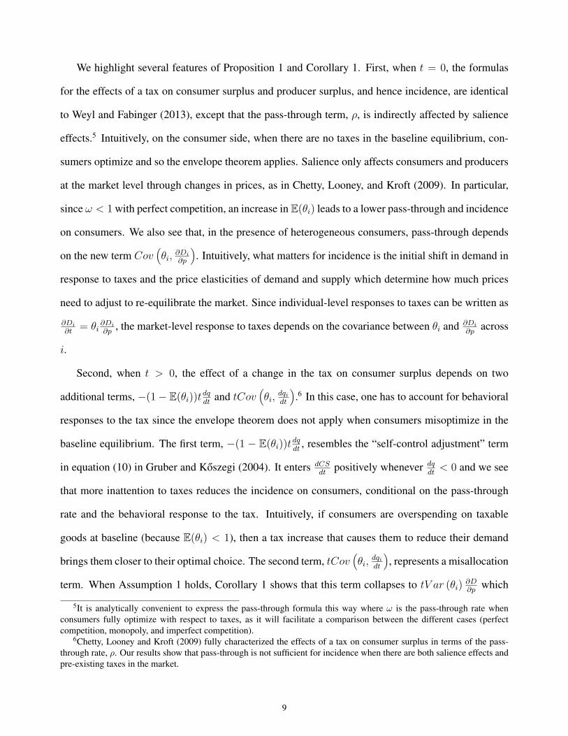
We highlight several features of Proposition 1 and Corollary 1. First, when t = 0, the formulas

for the effects of a tax on consumer surplus and producer surplus, and hence incidence, are identical

to Weyl and Fabinger (2013), except that the pass-through term, ρ, is indirectly affected by salience

effects.5 Intuitively, on the consumer side, when there are no taxes in the baseline equilibrium, con-

sumers optimize and so the envelope theorem applies. Salience only affects consumers and producers

at the market level through changes in prices, as in Chetty, Looney, and Kroft (2009). In particular,

since ω < 1 with perfect competition, an increase in E(θi) leads to a lower pass-through and incidence

on consumers. We also see that, in the presence of heterogeneous consumers, pass-through depends

on the new term Cov(θi,

∂Di∂p

). Intuitively, what matters for incidence is the initial shift in demand in

response to taxes and the price elasticities of demand and supply which determine how much prices

need to adjust to re-equilibrate the market. Since individual-level responses to taxes can be written as

∂Di∂t

= θi∂Di∂p

, the market-level response to taxes depends on the covariance between θi and ∂Di∂p

across

i.

Second, when t > 0, the effect of a change in the tax on consumer surplus depends on two

additional terms, −(1− E(θi))tdqdt and tCov(θi,

dqidt

).6 In this case, one has to account for behavioral

responses to the tax since the envelope theorem does not apply when consumers misoptimize in the

baseline equilibrium. The first term, −(1 − E(θi))tdqdt , resembles the “self-control adjustment” term

in equation (10) in Gruber and Koszegi (2004). It enters dCSdt

positively whenever dqdt< 0 and we see

that more inattention to taxes reduces the incidence on consumers, conditional on the pass-through

rate and the behavioral response to the tax. Intuitively, if consumers are overspending on taxable

goods at baseline (because E(θi) < 1), then a tax increase that causes them to reduce their demand

brings them closer to their optimal choice. The second term, tCov(θi,

dqidt

), represents a misallocation

term. When Assumption 1 holds, Corollary 1 shows that this term collapses to tV ar (θi) ∂D∂p which

5It is analytically convenient to express the pass-through formula this way where ω is the pass-through rate whenconsumers fully optimize with respect to taxes, as it will facilitate a comparison between the different cases (perfectcompetition, monopoly, and imperfect competition).

6Chetty, Looney and Kroft (2009) fully characterized the effects of a tax on consumer surplus in terms of the pass-through rate, ρ. Our results show that pass-through is not sufficient for incidence when there are both salience effects andpre-existing taxes in the market.

9

mirrors the expression in Taubinsky and Rees-Jones (2018) and Bernheim and Taubinsky (2018). If

consumers are fully attentive to the tax so that θi = 1 for all i, we see that dCSdt

and I are characterized

purely by the price effect, even with a pre-existing tax.

Third, independent of the baseline tax or the degree of inattention to the tax, when supply is

perfectly elastic (εS =∞), ρ = 1 and the full burden of the tax is on consumers so that I =∞.

Lastly, the marginal excess burden of the tax is scaled by the degree of inattention to the tax,

E(θi), and includes an additional term reflecting the dispersion in inattention, as in Taubinsky and

Rees-Jones (2018). In the case where θi = 0 for all i, taxes are not distortionary since with quasilinear

utility, the consumption allocation is the same as the consumption allocation with a lump-sum tax, as

shown in Chetty, Looney, and Kroft (2009). In the case where there is full pass-through (ρ = 1) and

homogeneous θi (E(θi) = θ), the marginal excess burden is a quadratic function of θ, dWdt

= θ2t∂D∂p

.

In the case where there are no pre-existing taxes, introducing a small tax into a market with or without

salience effects has no first-order effect on welfare.

3 Imperfect Competition

3.1 Monopoly

In this section, we depart from the benchmark case of perfect competition and consider a model of

imperfect competition. In order to develop intuition, we begin with the special case of monopoly.

We assume that the monopolist’s cost of production is given by c(q), with marginal cost mc(q) ≡

c′(q), and we define εS ≡ c′(q)c′′(q)q , which follows the definition in Weyl and Fabinger (2013). When

consumers are identical, the monopoly problem is particularly simple since in this case, θ(p, t) = θt

and D(p+ θt, 0) = D(p, t) and we may express the inverse demand function facing the firm as

P (q, t) = wtp(q)−θt, where wtp(q) is the inverse of D(·, 0). The monopolist’s problem in this case

can be stated as:

maxq

(wtp(q)− θt) q − c(q)

10

The first-order condition for the monopoly problem is wtp′(q)q+wtp(q)−θt = mc(q). In this

case, mr(q) = wtp′(q)q+wtp(q) is shifted down by θt. If the tax was fully non-salient so that θ = 0,

then consumer demand is not affected by taxes.

In the general case with consumer heterogeneity, we follow the setup from last section where for

each i, Di(p+θit, 0) = Di(p, t), and D(p, t) ≡∫Di(p, t)di. As before, the market demand elas-

ticity is defined as εD ≡ −∂D(p,t)∂p

p+tD

. We now introduce several new definitions which are relevant

for characterizing incidence and efficiency under imperfect competition. First, we define the rep-

resentative agent’s willingness to pay wtp(q) as the inverse of D(·, 0).7 Next, define the marginal

willingness to pay as mwtp(q) ≡ wtp′(q). Then ms(q) ≡ −mwtp(q)q is marginal consumer sur-

plus and the elasticity of inverse marginal surplus is given by εms ≡ ms(q)ms′(q)q . Furthermore, define

MS(q, t) = − q∂D∂p

(p(t),t) = ms(q)mwtp(q(t))∗ ∂D

∂p(p(t),t) . Note that MS(q, 0) = ms(q), and define MSt ≡ ∂MS

∂t.

Finally, we assume that tax revenue R = tq and profits π are redistributed to the consumers as a

lump-sum transfer. The consumer treats profits and tax revenue as fixed when choosing consumption,

failing to consider the external effects on the lump-sum transfer. Given the assumption of quasilinear

utility, the consumer will choose to allocate the lump-sum transfer to the outside market y. Thus, total

welfare, W , is given by the sum of consumer surplus (CS), producer surplus (PS) and government

revenue (R).

W (p, t) =∫ui(qi(p, t))di−(p+t)q(p, t)︸︷︷︸

CS

+pq−c (q)︸︷︷︸PS

+ tq︸︷︷︸R

Given these definitions, we can now characterize the incidence and marginal excess burden of

taxes for monopoly.

Proposition 2. The incidence on consumers, producers, government, the pass-through rate and the

7Formally, there is no representative agent for the economy since even with quasilinear utility there is a problem ofaggregation given the misoptimization with respect to taxes. However, when t = 0 the economy admits a representativeagent (given that there are no income effects) and we use the inverse demand function of this representative agent tocharacterize average and marginal consumer surplus.

11

marginal excess burden of a unit tax, t, under monopoly may be expressed as:

dCS

dt= −ρq − (1− E(θi))t

dq

dt+ tCov

(θi,

dqidt

)

dPS

dt= −q

E(θi) +Cov

(θi,

∂Di∂p

)∂D∂p

dR

dt= q + t

dq

dt

ρ = 1− (1− ω)E(θi) +

Cov(θi,

∂Di∂p

)∂D∂p

+ ωMSt, where ω = 11 + εD

pp+t−1εS

+ 1εms

I = εDp+tqE(θi∂Di∂p

) (ρ+ (1− E(θi))t

p+ tεDt −

t

qCov

(θi,

dqidt

))

dW

dt= (p−mc(q) + E(θi)t)

dq

dt+ tCov

(θi,

dqidt

)




dCS

dt=− ρq − (1− E(θi))t

dq

dt+ tV ar (θi)

∂D

∂p

dPS

dt= −qE(θi)

ρ = 1− (1− ω)E(θi), where ω = 11 + εD

pp+t−1εS

+ 1εms

I = 1E (θi)

(ρ+ (1− E(θi))

t

p+ tεDt −

t

pV ar (θi) εD

)

dW


dq

dt+ tV ar (θi)

∂D

∂p

= (p−mc(q) + E(θi)t)∂D

∂p(ρ− 1 + E(θi)) + tV ar (θi)

∂D

∂p

Several interesting insights emerge from the analysis of salience and taxation under monopoly.

First, we note that the formula characterizing the effects of the tax on consumer surplus is identical

to the formula in the case of perfect competition. Note, however, that the inputs to the formula are

12

different under monopoly as we discuss below.

Next, we see that the effects of a tax on producer surplus is −q

E(θi) +Cov

(θi,

∂Di∂p

)∂D∂p

. Consider

first the case where θi = 1 for all i. Since the monopolist sets the price (and level of output), the effect

of a small change in taxes is simply the mechanical effect of the tax change which is given by output,

q. Consumer inattention attenuates the effect of taxes on producers since instead of consumer demand

falling by the amount of the tax change, it falls by this amount scaled by the degree of inattention

E(θi). The covariance term Cov(θi,

∂Di∂p

)incorporates the correlation between θi and ∂Di

∂pwhich

determines the market-level demand response to the tax. When Cov(θi,

∂Di∂p

)> 0, the incidence on

the monopolist is attenuated.8 This can be easily seen in the binary case where there are two types of

consumers: those who optimize and those who are fully inattentive to taxes. If those who optimize

are price inelastic and those who are inattentive are price elastic, then the monopolist earns higher

profit compared to the case where inattention is uncorrelated with price elasticity. In fact, it may be

optimal for the monopolist to fully disclose taxes (e.g., post tax-inclusive prices) if there are enough

consumers who are both highly price elastic and overreact to taxes (so that θi > 1).9 This result on

optimal disclosure of taxes relates to Veiga and Weyl (2016) on how firms can optimally use nonprice

product features to sort profitable from unprofitable consumers. Finally, we note that the formula

holds even when mc(q) is constant so that εS = ∞. This contrasts with perfect competition where

dPSdt

= 0 when εS =∞.

Third, there are interesting effects of salience on pass-through, ρ, which operate through the elas-

ticity of inverse marginal surplus, which is positive (negative) if demand is log convex (log concave).

In particular, unlike the case of perfect competition, the monopoly outcome may be associated with

8Since ∂Di

∂p < 0, this requires that consumers that are attentive to taxes are price inelastic; in other words, the absolutevalue of ∂Di

∂p is negatively correlated with θi. Note that DellaVigna and Gentzkow (2019) find that high-income storesface less price elastic consumers and Taubinsky and Rees-Jones (2018) find that θi is higher for higher income individuals.This evidence suggests that Cov

(θi,

∂Di

∂p

)> 0.

9Morrison and Taubinsky (2020) find that some consumers overreact to taxes but do not investigate whether this iscorrelated with their price elasticity of demand. To see why disclosure is never optimal when θi < 1 for all consumers,consider the case where the monopolist discloses taxes at some q∗. If the monopolist then shrouds taxes, it could still sellq∗ but at a higher price since the inverse demand curve with hidden taxes lies everywhere above the inverse demand curvewith salient taxes. Thus, there is a profitable deviation and so disclosure can never be optimal when all consumers areinattentive to taxes.

13

ω > 1 which implies that an increase in E(θi) raises incidence on consumers. To see this, consider the

case of constant marginal cost and suppose demand has constant pass-through form so that εms = −ε

(Bulow and Pfleiderer 1983) and θi = θ. Under these assumptions, ρ = 1− θ1−ε so that dρ

dθ= 1

ε−1 , and

so if demand is sufficiently convex, then dρdθ> 0 and increased attention to the tax makes consumers

worse off, in contrast to the logic in Chetty, Looney and Kroft (2009) under perfect competition.10 We

also see that the expression for ρ in the case of monopoly depends additionally on MSt. Up to first

order this term can be approximated by MSt ≈ −q( ∂D∂p )2Cov

(∂2Di∂p2 , θi

)(see Appendix). This new term

captures that when taxes change and consumers vary in their degree of inattention, this effectively

changes the slope of the demand curve. Since the optimal price depends on the slope of the demand

curve, the monopolist exploits this change in market power when re-optimizing prices. If more atten-

tive consumers become more price elastic when taxes change, then Cov(∂2Di∂p2 , θi

)< 0 and MSt > 0.

Intuitively, when the tax increases there is a reallocation of demand, whereby the negative output

response qi is bigger (in absolute value) for more attentive and price elastic consumers; in the case

where Cov(∂2Di∂p2 , θi

)< 0, the average (or market) demand becomes more inelastic as demand is real-

located to more inelastic and less attentive consumers. Therefore, pass-through increases (MSt > 0).

Depending on the magnitude of MSt, it is possible to get overshifting of taxes onto consumer prices,

even when the standard model predicts undershifting. Corollary 2 shows that this term vanishes under

Assumption 1.

Finally, conditional on dqdt

, the effects of salience on the marginal excess burden of the tax operate

in similar ways under perfect competition and monopoly through the terms E(θi)t and tCov(θi,

dqidt

).

However, under monopoly the marginal excess burden depends additionally on the markup, p−mc(q).

This implies that changes in the degree of inattention to taxes have larger effects on excess burden

in monopolistic markets as compared to perfectly competitive markets. To see this, note that we

can express dqdt

= ∂D∂p

(ρ − 1 + E(θi)) as shown in Corollary 2. Thus, salience enters linearly in the

welfare formula dWdt

and interacts directly with the markup. For example, with full pass-through and

10Note that even when εS =∞, the full incidence is not on consumers, unlike the case of perfect competition, althoughwe note that this result holds independent of salience effects.

14

homogeneous consumers, dWdt

= (p−mc(q)) θ ∂D∂p

+ θ2t∂D∂p

. Even when there are no pre-existing

taxes, there is still a pre-existing distortion due to imperfect competition and thus introducing a small

tax into the market has a first-order effect on welfare which scales with the degree of inattention to

taxes. This shows that even when “behavioral biases” have a second-order effect on social welfare in

competitive markets, they may have a first-order effect on welfare in markets where firms have market

power. Holding fixed the markup, however, as frictions are reduced (i.e., increasing the value of θ),

the excess burden of taxation is increased.

To summarize, the analysis of the incidence and welfare consequences of a tax for the special case

of monopoly suggests that the standard intuition for the case of perfect competition does not always

apply when firms have market power. Instead, there are interesting interactions between tax salience

and market structure. This motivates our analysis of tax salience in a more general model of imperfect

competition.

3.2 Symmetric Imperfect Competition

We consider a differentiated product market (the “inside market”) which is subject to a unit tax t on

each product in the market. Following Auerbach and Hines (2001) and Weyl and Fabinger (2013), we

assume that markets for other goods are perfectly competitive and are not subject to taxation. There

is a mass 1 of consumers each indexed by i with exogenous income Zi. For each i, preferences are

given by the quasilinear utility function ui(q1, . . . , qJ)+y, where qj is the quantity consumed of product

j = 1, . . . , J and y ∈ R is the numeraire (representing consumption in all the outside markets).11 We

assume that the subutility function, ui, which represents preferences for the differentiated products,

is strictly quasi-concave, twice differentiable, and symmetric in all of its arguments. The pre-tax (or

producer) price for product j is given by pj and the after-tax (or consumer) price is given by pj + t for

all j = 1, ..., J . We define ui(Qi) ≡ ui(Qi/J, . . . , Qi/J) to be the compact notation of utility for the

symmetric case where the individual consumes qi = Qi

Junits of each product j = 1, . . . , J , where Qi

11We now use a superscript to index individuals since there is an additional dimension of heterogeneity coming fromasymmetric products. We use the subscript j to index products.

15

is the aggregate quantity consumed by the individual.

Following Chetty, Looney and Kroft (2009), consumer i demand for product j is given by qij =

qij(p1, . . . , pJ , t) which is a function of both pre-tax prices and the tax. In order to connect our tax

formulas to empirical objects, it is necessary to relate observed demand qij(p1, . . . , pJ , t) to consumer

willingness to pay. We thus make the following assumptions which mirror assumptions A1 and A2 in

Chetty, Looney and Kroft (2009).

Assumption 2. Taxes affect utility only through their effects on the chosen consumption bundle. In-

direct utility is given by:

V i(p1, . . . , pJ , t, Zi) = ui(qi1(p1, . . . , pJ , t), . . . , qiJ(p1, . . . , pJ , t))+Zi−(p1 + t)qi1− ···−(pJ + t)qiJ

Assumption 2 requires that taxes or salience have no impact on utility beyond their effects on

consumption.

Assumption 3. When tax-inclusive prices are fully salient, the agent chooses the same allocation as

a fully-optimizing agent.

(qi1, . . . , qiJ)(p1 + t, . . . , pJ + t, 0) = arg max(q1,...,qJ )

ui(q1, . . . , qJ)+Zi−(p1 + t)q1− ···−(pJ + t)qJ

Assumption 3 implies that when tax-inclusive prices are fully salient, agents maximize utility.

As in Section 2 we allow for salience effects by considering the possibility that qij(p1, ..., pJ , 0) >

qij(p1, ..., pJ , t) > qij(p1 + t, ..., pJ + t, 0).

In what follows, we assume that the demand function qij(·) is symmetric in all other prices which

we denote by (pk)−j and twice differentiable and denote by qi(p, t) demand corresponding to sym-

metric prices and J firms: qi(p, t) ≡ qij(p, ..., p, t). Without loss of generality on the functional form

of qi(·, 0) = (u′i)−1(·)J

, and we assume qi(p, t) = qi(p+θit, 0) for some θi > 0; therefore, the salience

parameter satisfies θi =∂qij

∂t∂qij

∂p

and is the same for all products j for individual i.

We define individual i’s market demand asQi(p, t) = Jqi(p, t). Total market demand is then given

by Q(p, t) =∫Qi(p, t)di, from where we define the market demand elasticity εD ≡ −∂Q(p,t)

∂pp+tQ

.

Also, for an economy without taxes, we define the representative agent’s willingness to pay wtp(Q)

16

as the inverse of Q(·, 0), and let mwtp(Q) = wtp′(Q) be the marginal willingness to pay. Then

ms(Q) = −mwtp(Q)Q is the marginal consumer surplus and the elasticity of inverse marginal sur-

plus is given by εms ≡ ms(Q)ms′(Q)Q . Furthermore, define MS(Q, t) = − Q

∂Q∂p

(p(t),t)= ms(Q)

mwtp(Q(t))∗ ∂Q∂p

(p(t),t),

then MS(Q, 0) = ms(Q), and let MSt ≡ ∂MS.

Let qj(p1, ..., pJ , t) =∫qij(p1, ..., pJ , t)di. On the supply side, we allow for different forms of

competition by introducing the market conduct parameter νp = ∂pk∂pj

(k 6= j) following Weyl and

Fabinger (2013). Assume each firm produces a single product and has cost function cj(qj) = c(qj),

where c(·) is increasing and twice differentiable with c(0) = 0 and mc(qj) ≡ c′(qj). Firm j chooses

pj to maximize profits πj:

maxpj

πj = pjqj(p1 . . . , pJ , t)− c(qj(p1 . . . , pJ , t))

s.t.∂pk∂pj

= νp for k 6= j

The first-order condition for pj is given by:

qj+(pj−mc(qj))∂qj∂pj

+νp∑k 6=j

∂qj∂pk

= 0.

In a symmetric equilibrium, pj = p solves:

qj(pj, p, . . . , p, t)+(pj−mc(qj))(∂qj(pj, p, . . . , p, t)

∂pj+(J−1)νp

∂qj(pj, p, . . . , p, t)∂pk

)= 0, k 6= j

We assume that ∂πj∂pj

(pj, p) is strict single crossing (from above) in pj and decreasing in p so that a

unique symmetric equilibrium p(t) exists.12 By letting νq = 1mwtp(Q)×

1dqjdpj

= 1mwtp(Q)×

1∂qj∂pj

+νp∑

k 6=j∂qj∂pk

we can rewrite the first-order condition as a generalized Lerner index:

p−mc(q)p+ t

= νqJεD

(1)

Setting νq = J yields the monopoly (perfect collusion) outcome and setting νq = 0 gives the perfect

competition (marginal cost pricing) solution. Setting νq = 1 corresponds to Cournot competition

when goods are homogeneous and setting νp = 0 yields the Bertrand-Nash equilibrium. The model

12The case of strategic complementarities, where ∂πj

∂pj(pj , p) is increasing in p allows for the existence of multiple

symmetric equilibria. However, in that case if we assume there is a continuous and symmetric equilibrium selection p(t)the same results follow.

17

thus captures a wide range of market conduct.

We assume that tax revenue R = tQ and profits Jπ are redistributed to the consumers as a lump-

sum transfer. The consumer treats profits and tax revenue as fixed when choosing consumption,

failing to consider the external effects on the lump-sum transfer. Given the assumption of quasilinear

utility, the consumer will choose to allocate the lump-sum transfer to the outside market y. Thus, total

welfare, W , is given by the sum of consumer surplus (CS), producer surplus (PS) and government

revenue (R).

W (p, t) =∫ui(Qi(p, t))di−(p+t)Q(p, t)︸︷︷︸

CS

+pQ−Jc (q)︸︷︷︸PS

+ tQ︸︷︷︸R

We can now state our main result. Consider a small increase in the tax t which applies to all goods

in the inside market.

Proposition 3. The incidence on consumers, producers, government, the pass-through rate and the

marginal excess burden of a unit tax, t, under symmetric imperfect competition may be expressed as:

dCS

dt= −ρQ− (1− E(θi))t

dQ(p(t), t)dt

+ tCov

(θi,

dQi(p(t), t)dt

)

dPS

dt= −

(1− νq

J

)[Q(1− ρ)]− νq

J

QE(θi) +

Cov(θi,

∂Qi

∂p

)∂Q∂p

dR

dt= Q+ t

dQ(p(t), t)dt

ρ = 1− (1− ω)E(θi) +

Cov(θi,

∂Qi

∂p

)∂Q∂p

+ ωνqJMSt where ω = 1

1 + εDpp+t−

νqJ

εS+

νqJ

εms

I =ρ+ (1− E(θi)) t

p+tεDt −tQCov

(θi,

dQi(p(t),t)dt

)(1− ρ)

(1− νq

J

)+ νq

J

E(θi∂Qi

∂p

)E(∂Qi

∂p

)dW


dQ(p(t), t)dt

+ tCov

(θi,

dQi(p(t), t)dt

)



18


dCS

dt=− ρQ− (1− E(θi))t

dQ(p(t), t)dt

+ tV ar (θi)∂Q

∂p

dPS

dt=−Q

[(1− νq

J

)(1− ρ) + νq

JE(θi)

]

ρ = 1− (1− ω)E(θi), where ω = 1

1 + εDpp+t−

νqJ

εS+

νqJ

εms

I =ρ+ (1− E(θi)) t

p+tεDt −tp+tV ar (θi) εD

(1− ρ)(1− νq

J

)+ νq

JE(θi)

dW


dQ(p(t), t)dt

+ tV ar (θi)∂Q

∂p

= (p−mc(q) + E(θi)t)∂Q

∂p(ρ− 1 + E(θi)) + tV ar (θi)

∂Q

∂p

Proposition 3 leads to several additional insights. First, dCSdt

has the same expression as perfect

competition and monopoly. Thus, the change in consumer surplus does not depend directly on market

conduct, except insofar as market conduct determines pass-through. Second dPSdt

is a convex combi-

nation of the monopoly and perfect competition cases with weights νqJ

and 1 − νqJ

, respectively. To

understand this expression, note that when θi = 1 for all i, dPSdt

= −Q((1−ρ)+ρνq

J

), similar to Weyl

and Fabinger (2013). When firms have market power, they internalize the change in their own output

on the market (given by νqJ

), and so we need to adjust the price effect by ρνqJ

. Under monopoly, this

effect becomes ρ and dPSdt

= −Q. Similar to monopoly, if firms have market power, then salience

directly attenuates the reduction in demand due to taxes and thus reduces the tax burden on producers.

We again see that in the general case, there are interesting effects of salience on pass-through

depending on the magnitudes of νq and εms. As in the monopoly case, greater attention to taxes

can increase the burden on consumers if there is overshifting of taxes, again illustrating that salience

and the degree of competition interact in determining the relative incidence of taxes on consumers

and producers. In the simpler case of Corollary 3, the only role that salience plays is attenuating

the initial response of consumer demand to a change in taxes. The intuition for this result is that,

conditional on the demand response to taxes, salience does not directly affect the equilibrium response

19

of prices. Conditional on this response, the firm’s equilibrium response to the tax is determined purely

by standard forces such as the marginal cost function, the shape of the demand curve and market

conduct. Mathematically, this is because ω depends on supply and demand fundamentals and the

conduct parameter. Salience only affects the weighting on ω in the expression for ρ. Thus, conditional

on ω, the role of salience in affecting pass-through will be similar whether firms have a lot of market

power (as in Monopoly) or only a little bit of market power (as in Bertrand or Cournot). However, in

Proposition 3 we see that the expression for ρ depends additionally on ω νqJMSt. Like in monopoly,

this term can be approximated byMSt ≈ −Q( ∂Q∂p )2Cov

(∂2Qi

∂p2 , θi)

(see Appendix), but now it is weighted

by νqJ

— the relative distance of firm behavior to the monopoly benchmark. In the previous section

we explain how this term captures that when taxes change, because consumers vary in their degree of

inattention, there is a reallocation effect that effectively changes the elasticity of the demand curve.

Finally, we see that the marginal excess burden formula depends on the same set of sufficient statis-

tics as in the monopoly case. In particular, the conduct parameter does not appear in the formula, and

thus the intuition for welfare in the monopoly case carries over to the general model. Intuitively, the

marginal excess burden of taxes is the lost social surplus that accrues from discouraging transactions

in which the value of the product exceeds the cost of production. The marginal value of product with

quasilinear utility is simply p + E(θi)t. The marginal cost of production is mc(q). The discouraged

transactions is represented by dQ(p(t), t)/dt and we have the misallocation term which depends on

V ar(θi). Note that price effects do not show up in the formula since they are transfers between con-

sumers and firms. Of course, the inputs to the formula, such as p and mc(q), will depend on market

conduct, but conditional on them, conduct does not independently affect the marginal excess burden.

4 Ad Valorem versus Unit Taxes

It is well known that ad valorem and unit taxes are not equivalent in imperfectly competitive markets

(Delipalla and Keen 1992, Anderson, de Palma and Kreider 2001a, Adachi and Fabinger 2019). This

section extends our results on incidence and excess burden in Proposition 3 to ad valorem taxes in the

20

presence of salience effects. We consider the model of imperfect competition with both unit taxes and

ad valorem taxes. The purpose of the model is to compare the incidence and welfare effects of these

taxes and to forge a link with the empirical section which considers ad valorem taxes. For ease of

exposition, we assume identical consumers and present the general expressions for ad valorem taxes

in the presence of heterogeneous consumers that we calibrate in Section 6.

Let p denote the producer price and let p(1 + τ) + t denote the price paid by consumers where

τ is the ad valorem tax and t is the unit tax. Demand is given by D(p, t, τ) and assume that for

τ > 0 and t > 0, D(p, 0, 0) > D(p, t, τ) > D(p(1 + τ) + t, 0, 0). For any triple (p, t, τ) there exists

θτ (p, t, τ) and θt(p, t, τ) to be such that: D(p, t, τ) = D(p(1 + θττ) + θtt, 0, 0). However following

the literature and to simplify the setup assume θτ and θt are independent of the level of prices and tax

rates. Equivalently we could define θτ ≡∂D∂τ∂D∂p

× 1p

and θt ≡∂D∂t∂D∂p

and assume they are constant with

respect to prices and taxes.13 Following the prior section, we extend the definition of willingness to

pay to accommodate the ad valorem tax so that wtp(Q) = p(1 + θττ) + θtt.

Let εD ≡ −∂Q∂p

p(1+τ)+tQ

, ε∗D = εDp

p(1+τ)+t and define the pass-through rates for ad valorem and

unit taxes respectively, as ρτ ≡ 1p∂(p(1+τ)+t)

∂τand ρt ≡ ∂(p(1+τ)+t)

∂t. The following lemma shows how

to identify θτ with commonly observable objects.

Lemma 2. Let εDτ ≡ dQdτ

p(1+τ)+tQ

. The following relationship holds:

εDτ = −εD ∗p

1 + τ((1 + θττ) ρτ + θτ − 1)

and

θτ = (1− ρτ ) pεD − εDτ (1 + τ)(1 + τρτ ) pεD


With Lemma 2 in hand, we can now state our main proposition for ad valorem taxes. Following the

literature, we compare the pass-through rates and the marginal cost of public funds. A lower marginal

13Note that in the denominator of θτ and θt, the derivative is with respect to the first argument of D.

21

cost of public funds indicates greater efficiency. We begin with the characterization of pass-through

rates.

Proposition 4. In the symmetric model of imperfect competition, the pass-through rates for ad val-

orem and unit taxes are given respectively as:

ρτ = 1− (1 + τ)θτ1 + θττ

(1− ωmc(q)

p

)

ρt = 1− (1 + τ)θt1 + θττ

(1− ω)

where ω = 1

1+(1+θτ τ)ε∗

D−νqJ

εS+ νqJ

1εms

.

This implies that the two pass-through rates can be ranked based on the following:

ρτ − 1ρt − 1 = θτ

θt

ωmcp− 1

ω − 1 = θτθt

(1− ω

ω − 1νqJε∗D

)


A first observation is that when θτ = θt, if mc < p then ρτ < ρt which is consistent with the

literature (Delipalla and Keen 1992; Adachi and Fabinger 2019). Thus, if consumers underreact to

ad valorem and unit taxes similarly, the pass-through rate is lower for ad valorem taxes. A new

observation is that even under perfect competition starting from p = mc, ad valorem taxes imply a

higher pass-through than unit taxes ρt < ρτ if and only if the consumers are more responsive to ad

valorem taxes than unit taxes θτ > θt.14 Most of the available empirical evidence in the literature

applies to sales taxes and thus, θτ . Our results stress the need for additional evidence on θt.

Next, we derive the marginal cost of public funds for an ad valorem tax and a unit tax which are

defined as MCτ ≡ −dW/dτdR/dτ

and MCt ≡ −dW/dtdR/dt

, respectively.

Proposition 5. Denote wtp = p(1 + θττ) + θtt the perceived price by the consumer and ε∗D =

εDp

p(1+τ)+t . The marginal cost of public funds for an ad valorem tax, τ , and a unit tax, t, under

14As a basic matter of tax administration, this is relatively unlikely. Indeed, it has been suggested to us that the relativesaliency of unit taxes appears to have played an important role in dictating the implementation details of recently-adoptedbeverage taxes.

22

symmetric imperfect competition may be expressed as:

MCτ = ε∗D

wtp−mcp

1+τρτ(1+θτ τ)ρτ+θτ−1 − ε

∗D(τ + t

p)

MCt = ε∗D

wtp−mcp

1+τρt(1+θτ τ)ρt+θt−1 − ε

∗D(τ + t

p)

This implies the following:

MCtMCτ

=1+τρτ

(1+θτ τ)ρτ+θτ−1 − ε∗D(τ + t

p)

1+τρt(1+θτ τ)ρt+θt−1 − ε

∗D(τ + t

p)

In other words, the cost of ad-valorem taxes is lower than the cost of unit taxes (MCτ < MCt) if

and only if

θτ

[1− 1 + τ(1 + θτ − θt)

1 + θττ

(1− ωmc

p

)]< θt

[1− 1 + τ

1 + θττ(1− ω)

]


It is instructive to consider the benchmark case where θτ = θt. In this case, MCτ < MCt if and

only if p > mc. Thus, as long as consumers respond symmetrically to ad valorem and unit taxes, then

salience does not affect the well-known result that ad valorem taxes are more efficient than unit taxes

under imperfect competition. Of course, if consumers are sufficiently more attentive to ad valorem

taxes than unit taxes, then this result shows that ad valorem taxes can be more distortionary than unit

tax.

5 Data and Estimation

5.1 Data Description

Nielsen Retail Scanner Data We measure prices and quantity using the Nielsen Retail Scanner

(RMS) data from 2006 − 2014. This data set records sales and the number of units sold per week

for roughly 2.5 million products which are designated as Universal Product Codes (UPC) for 35,000

stores in the United States (excluding Hawaii and Alaska) that are part of roughly 90 retail chains.

23

The UPCs are organized by Nielsen according to a hierarchical structure.15 At the lowest rung

are approximately 1,200 product-modules (e.g., fresh eggs, chocolate candy, olive oil, bleach, toilet

tissue). Each module is assigned to one of roughly 120 product-groups (e.g. candy, shortening and

oil, laundry supplies, paper products). These groups belong to one of 10 broader product-departments

(e.g., dry grocery, fresh produce, non-food grocery). Stores are assigned to one of five possible store

types: grocery, drug, mass merchandise, convenience, and liquor stores. Each store has a “parent

company” that corresponds to the company that owns the store, and the data also indicates when

multiple stores are part of the same retail chain.

We limit our sample to grocery stores for two reasons. First, the distribution of store types varies

considerably across counties. By focusing on one store type, we ensure that compositional differences

across counties are not driving our results. Second, we use an instrumental variables strategy which

relies on uniform pricing within retail chains following DellaVigna and Gentzkow (2019). There

are too few retail chains for non-grocery stores, making this strategy infeasible these store types. We

follow DellaVigna and Gentzkow in further restricting our sample to (1) stores that belong to the same

retail chain throughout 2006−2014, (2) stores that are present in the data for at least two years, and (3)

stores that belong to retail chains that were associated with the same parent company throughout the

sample period. In terms of products, we keep all products in modules that are sold in all 48 continental

states and we restrict the sample to top-selling modules that rank above the 80th percentile of total

U.S. sales. These 198 modules account for almost 80 percent of the total sales in grocery stores in the

Nielsen data.16

The key variables for our empirical analysis are price and quantity. We define these variables at

the level of module (m), store (r), and time (n), where a unit of time is a year-quarter. This requires

aggregating weekly revenue and quantities sold separately for each product to the quarterly level. A

quarterly price is obtained by dividing quarterly revenue from the sales of product j by the number

15Appendix Table OA.1 describes the hierarchy of the data using example UPCs. UPCs without a barcode such asrandom weight meat, fruits, and vegetables are excluded from our sample.

16We limit to the top 20 percent of modules for computational reasons, and we have explored some of our mainspecifications in the full sample of modules and found very similar results (results not reported).

24

of units sold in that quarter. To address the concern that there may be compositional differences in

price across stores due to different UPCs being offered, we follow Handbury and Weinstein (2015)

and regress log quarterly price on UPC fixed effects and module-by-store-by-time fixed effects. The

module-by-store-by-time fixed effects serve as the pre-tax price for the purpose of estimation. To

measure quantity, we create a price-weighted quantity index based on the national price of products.17

Specifically, for each product (j), store (r) and time (n), we multiply quantity purchased by the

average national price (across all stores in our sample) of product j at time n, where the national price

is an unweighted average. We then aggregate quantity across products within a module-by-store-by-

time cell to arrive at a quantity measure that varies at the same level as the price index.

U.S. Sales Tax Exemptions and Rates We collect data on local (county and state) sales tax rates

and tax exemptions from a variety of sources, including state laws, state regulations, and online

brochures.18 In general, tax exemptions are set by U.S. states and are module-specific. The general

rule of thumb is that states exempt food products from taxation and tax non-food products. However,

there are several important exceptions to this rule which are reported in Table 1. First, several states

tax food at the full rate or a reduced rate. Second, in a few states, food products are exempt from the

state-level portion of the total sales tax rate, but remain subject to the county-level sales tax.19 Third,

in some cases where food is tax-exempt, there is a tax that applies at the product-module level. For

example, prepared foods, soft drinks, and candy are subject to sales taxes in many states. Finally,

some states exempt some non-food products from sales taxes. As a result, the effective sales tax rate

varies by module (m), county (c), and time (n).20

17This normalization by the national price allows us to compare quantities across different goods and modules, andsince all of our specifications include module-by-time fixed effects, the quantity measure is implicitly normalized relativeto the module-by-time mean. In other words, explicitly normalizing the quantity measure by the national average priceacross products within a module-by-time cell leads to identical results.

18All data sources used to determine the exemption status of products are listed in Appendix Table OA.2.19Colorado, for example, allows each county to decide whether to subject food to the county-level portion of the sales

tax rate.20The Online Appendix shows the cross-sectional variation in sales tax rates and sales tax exemptions in our data.

Appendix Figure OA.1 reports the total (state + county) sales tax rate in September 2008 and shows tax rates rangingfrom 0 in Montana, Oregon, New Hampshire and Delaware to a maximum rate of 9.75 percent in Tennessee. AppendixFigure OA.2 reports the food tax exemptions across states and shows that many of the states that tax food are located in

25

There are two potential sources of measurement error in our sales tax rates. First, we do not

incorporate county-level exemptions or county-specific sales surtaxes that apply to specific products

or modules, although our understanding is that these cases are uncommon. Second, in some cases,

there is some discretion in how we assign a taxability status to each module, based on interpreting the

text of a state’s sales tax law. While the bulk of the variation in taxes occurs at the module level or

higher, there are some instances where taxability varies within module. For example, in New York,

fruit drinks are tax exempt as long as they contain at least 70% real fruit juice, but are subject to the

sales tax otherwise. Therefore, some products in Nielsen’s module “Fruit Juice- Apple”, may or may

not be taxed in New York, but we code these products as tax exempt since we cannot readily identify

the real fruit juice content. In cases where it is impossible to tell whether the majority of products in

a given module are subject to the tax or not, we code the statutory tax rate as missing. This results in

excluding less than 3 percent of the observations in our sample.

Overall, we are confident that we have measured sales tax rates with a high degree of accuracy.

While sales tax exemptions are important for ensuring accurate measurement, the identifying variation

in our emprical analysis comes primarily from changes in sales tax rates within counties over time.

Changes in exemptions are very rare during our sample period, and all of our main specifications

include module-by-state-by-time fixed effects, so any changes in state sales tax rates or tax exemptions

(regardless of the set of modules affected) are absorbed into these fixed effects and thus not used for

identification of the effects of sales taxes.

Matched Sample As a last step in constructing our analysis sample, we merge the tax data onto the

Retail Scanner data. The stores in the Nielsen data are geolocated at the county level so we conduct

the merge at the level of module (m), county (c) and time (n). To measure the sales tax rate by quarter

of year, we use the tax rate effective at the mid-point of each quarter (February for quarter 1, May for

either the South or the Midwest. Appendix Figure OA.3 shows the changes in sales tax rates between Q1 2006 and Q42014, since our main results are based on local variation in sales tax rates over time (rather than cross-sectional variationacross states and counties at a point in time). This figure shows that there is still meaningful variation in sales taxes withincounties over time during this time period, including both increases and decreases in sales tax rates. Appendix FigureOA.4 shows the number of tax changes within counties during the same time period.

26

quarter 2, etc). We have also tried using the quarterly average of monthly sales tax rates and found

that our estimates were almost identical. Our final sample includes 8,652 grocery stores, and includes

price, quantity and tax rates for 198 modules in 1,460 counties over 36 year-quarters.

5.2 Estimation Strategy

The Effect of Taxes on Prices and Quantity Our main specification is a “constant effects” model

which can be derived from the model above by assuming that consumers have identical demand func-

tions. We estimate the effect of sales taxes on consumer prices and quantity using two complementary

regression models. The first model uses the full set of counties from the Neilsen Retail Scanner data

using the following estimating equation:

log ymrn = βy log(1+τmcn)+δmsn+δmr+εmrn (2)

where the outcome ymrn is either consumer prices (p(1 + τ)) or quantity (Q) for module m, store r

and time n. The term τmcn is the sales tax rate that applies to module m in county c at time n. The

terms δmsn and δmr are module-by-state-by-time and module-by-store fixed effects, respectively. The

identifying assumption is that changes in sales taxes do not change within counties in ways that are

correlated with changes in consumer demand (conditional on the fixed effects). This model allows

for arbitrary trends across states and modules and thereby relies on within-county-over-time variation

in tax rates. The estimate βy can be interpreted as the elasticity of prices or quantity with respect to

taxes (βp(1+τ) and βQ, respectively).

The second regression model uses a subsample of counties and a “county border pair” research

design, following Holmes (1998) and Dube, Lester and Reich (2010). This alternative approach

identifies the effects of sales taxes using pairs of counties on opposite sides of a state border and is

designed to address the concern that sales tax rates are endogenous to local economic conditions.

Under the assumption that local economic conditions are similar within a pair of border counties, the

effects of sales tax rates can be identified through “local” comparisons within each county border pair.

27

As a result, for this analysis we restrict the sample to stores located in contiguous counties on opposite

sides of a state border. Two contiguous counties located in different states form a county-pair d, and

counties are paired with as many cross-state counties as they are contiguous with. The estimating

equation is the following:

log ymrn = βy log(1+τmcn)+δ′mdn+δ′mr+ε′mrn. (3)

where δ′mdn and δ′mr are module-by-border-pair-by-time and module-by-store fixed effects, respec-

tively. This specification includes flexible trends for each module in each border pair. To estimate

equation (3), the original dataset is rearranged by stacking all county pairs and weighting each store

by the inverse of the number of times it is included in a border pair. In this regression model, the

identifying assumption is that within a border pair, variation in tax rates for a given module over time

is not correlated with other unobserved determinants that differentially affect one of the counties in

the pair. One way this assumption could fail is if counties adjust their tax rates based on economic

conditions within the border pair. To address this concern, we also report results in Appendix Table

OA.3 in which we instrument the total tax rate with the state sales tax rate (and find similar results).

The main results from estimating equations (2) and (3) are reported in Panel A of Table 2. Standard

errors are clustered by state-module and reported in parentheses.21 The first column uses the full

sample, and the second column uses the “border pair” subsample. The first row reports results for log

consumer prices. In column (1), the coefficient estimate βp(1+τ) = 0.961 (s.e. 0.045) indicates a large

but incomplete amount of pass-through of taxes onto consumer prices.22 The next row reports the

estimate βQ = −0.668 (s.e. 0.185), indicating a meaningful quantity response to tax changes. The

results in column (2) show similar results using the county border pair approach. The similar results

across the columns is consistent with limited endogeneity bias in the full sample.23

21Clustering by state-module is more conservative than clustering by state-by-module-time. The pass-through estimatesare based on a module-level price index which is a generated regressor, but for computational reasons, we ignore theuncertainty in this generated regressor and treat it as measured without error. The primary uncertainty we want to accountfor in our statistical inference is the design-based uncertainty from state and local policy changes that affect sales tax rates.

22Classical measurement error in effective tax rates biases our estimates of βp(1+τ) towards 1. Instrumental variableestimates of the effect of sales taxes on prices presented in Appendix Table OA.1 are slightly smaller than their corre-sponding border-sample OLS estimates, suggesting a small amount of attenuation bias.

23The minimum wage literature has also tended to find that results using all counties and “traditional” fixed effects

28

Tax salience parameter Since the main specification is a “constant effects’” specification with no

heterogeneity across consumers in terms of demand responses, there is no heterogeneity in the tax

salience parameter, θτ . In this setup, to estimate the tax salience parameter θτ , the effect of sales

taxes on quantity needs to be scaled by the effect of price changes on quantity. To estimate the

price elasticity of demand, we follow the recent literature on uniform pricing by retail chains and

construct a store-level instrument based on the pricing of products of other stores in a given retail

chain (DellaVigna and Gentzkow 2019). This instrumental variables strategy relates to earlier work

by Hausman (1996) and Nevo (2001), and has been used in several recent papers (e.g., Atkin, Faber

and Gonzalez-Navarro 2018 and Allcott et al. 2019).

Specifically, we construct an instrument zmrn that is equal to the average log pre-tax price across

all stores in the same retail chain excluding store r:

zmrn =∑x∈f log(pmxn)− log(pmrn)

Nfn − 1

where f denotes the retail chain to which store r belongs and Nfn is the number of stores in chain

f at time n. This is a valid instrument under the assumption that chain-level prices predict “own”

store prices, but are not correlated with unobserved store-level demand determinants. A threat to the

validity of this instrument is that there are correlated demand shocks across stores within retail chains.

To address this, we continue to include store-by-module fixed effects in all of our specifications.

The inclusion of module fixed effects accounts for the fact that more expensive modules may reflect

chains responding to strong demand for these modules. Intuitively, our identification is coming from

differences in relative prices across modules and chains. To the extent that this variation is driven by

differences in product-specific marginal costs across chains, differences in distribution costs across

chains (such as supply-sourcing costs), or differences in bargaining power across chains, we can

consistently estimate our elasticity of interest, since these supply-side instruments will identify the

average price elasticity of demand. Intuitively, this approach requires that chains select store locations

based on overall demand factors (that are common across modules), but not module-specific demand

models are similar to results based on the county border pair approach (see, e.g., Dube, Lester, and Reich 2010).

29

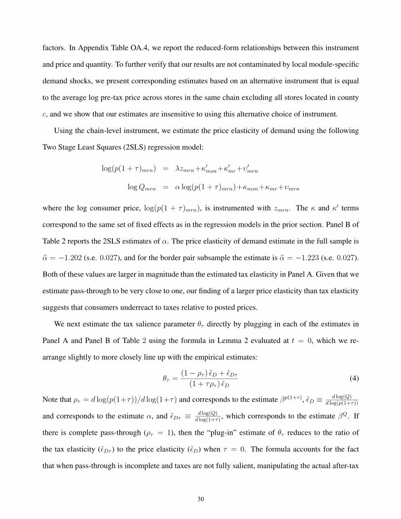
factors. In Appendix Table OA.4, we report the reduced-form relationships between this instrument

and price and quantity. To further verify that our results are not contaminated by local module-specific

demand shocks, we present corresponding estimates based on an alternative instrument that is equal

to the average log pre-tax price across stores in the same chain excluding all stores located in county

c, and we show that our estimates are insensitive to using this alternative choice of instrument.

Using the chain-level instrument, we estimate the price elasticity of demand using the following

Two Stage Least Squares (2SLS) regression model:

log(p(1 + τ)mrn) = λzmrn+κ′msn+κ′mr+υ′mrn

logQmrn = α log(p(1 + τ)mrn)+κmsn+κmr+υmrn

where the log consumer price, log(p(1 + τ)mrn), is instrumented with zmrn. The κ and κ′ terms

correspond to the same set of fixed effects as in the regression models in the prior section. Panel B of

Table 2 reports the 2SLS estimates of α. The price elasticity of demand estimate in the full sample is

α = −1.202 (s.e. 0.027), and for the border pair subsample the estimate is α = −1.223 (s.e. 0.027).

Both of these values are larger in magnitude than the estimated tax elasticity in Panel A. Given that we

estimate pass-through to be very close to one, our finding of a larger price elasticity than tax elasticity

suggests that consumers underreact to taxes relative to posted prices.

We next estimate the tax salience parameter θτ directly by plugging in each of the estimates in

Panel A and Panel B of Table 2 using the formula in Lemma 2 evaluated at t = 0, which we re-

arrange slightly to more closely line up with the empirical estimates:

θτ = (1− ρτ ) εD + εDτ(1 + τρτ ) εD

(4)

Note that ρτ = d log(p(1+τ))/d log(1+τ) and corresponds to the estimate βp(1+τ), εD ≡ d log(Q)d log(p(1+τ))

and corresponds to the estimate α, and εDτ ≡ d log(Q)d log(1+τ) , which corresponds to the estimate βQ. If

there is complete pass-through (ρτ = 1), then the “plug-in” estimate of θτ reduces to the ratio of

the tax elasticity (εDτ ) to the price elasticity (εD) when τ = 0. The formula accounts for the fact

that when pass-through is incomplete and taxes are not fully salient, manipulating the actual after-tax

30

price is not the same as manipulating the perceived price. Similar to other estimation approaches

in the literature, our identification of θτ relies on consumers perceiving tax and price changes to be

equally persistent, such that there is no difference in the degree of intertemporal substitution under

full salience. Similarly, it requires that equivalent price and tax changes induce the same degree of

substitution between product-modules.

Panel C of Table 3 reports our “plug-in” estimates of θτ using our reduced-form results and using

τ = 0.036, which is the sample average sales tax rate. We estimate θτ = 0.575 (s.e. 0.147) using

the full sample and θτ = 0.528 (s.e. 0.130) using the border-pair subsample.24 For comparison,

Chetty, Looney and Kroft (2009) estimate θτ = 0.35 using a field experiment which posted tax-

inclusive prices in a grocery store. Taubinsky and Rees-Jones (2018) and Morisson and Taubinsky

(2020) conduct online shopping experiments in which participants face different tax rates on common

household goods. Using experimental variation in tax rates along with a pricing mechanism used to

elicit willingness to pay, they report ranges of experimental estimates of θτ between 0.23 and 0.54

and between 0.23 and 0.79, respectively.

As a robustness test, we consider an alternative method for calculating the tax elasticity and the

price elasticity, as well as the associated value of θτ , in Appendix Table OA.6. In Panels A and

B, we report the effect of taxes and of the price instrument on total expenditures.25 We then back

out the implied effect on quantity by subtracting the effect on prices (column 2) from the effect on

expenditures (column 3). The implied values of the average tax salience parameter are θτ = 0.552

and θτ = 0.491 for the full sample and the border-pair subsample, respectively.

24Appendix Table OA.5 presents results based on alternative ways to account for spatial heterogeneity in consumptiontrends in our main sample. To account for county-level time-varying heterogeneity, we parameterize country-specifictrends for each module as linear time trends (module-by-county-by-year-quarter fixed effects leave no residual variationin tax rates and therefore cannot be used). We also consider store-specific linear trends for each module. The tax and priceelasticities under these alternative specifications are smaller than our preferred estimates and imply slightly lower valuesof θτ , ranging between 0.376 and 0.507. We note that the inclusion of module-by-state-by-year-quarter fixed effects in ourpreferred specification effectively shuts down variation from state-level tax rates, whereas county-module linear trends donot.

25Total expenditures on modulem is equal to∑j∈m (qjrn × pjrn), where j denotes a UPC. The effect on expenditures

therefore captures both the effects on prices and on quantity.

31

6 Calibrations

In this section, we calibrate the incidence and marginal excess formulas for ad valorem taxes using

the estimates in the previous section. We then compute the difference between our marginal excess

burden formula and the standard Harberger formula and decompose it into the deviation coming from

salience effects and the deviation coming from imperfect competition. Lastly, we consider counter-

factual scenarios that increase tax salience and change the market structure, taking into account the

endogeneity of the output response to the tax and the pass-through rate with respect to tax salience

and market structure. These scenarios reveal the various interactions between tax salience and imper-

fect competition in determining the pass-through of taxes into consumer prices, the effect of taxes on

quantity demanded, and ultimately the incidence and marginal excess burden.

To begin, we recover the markup and the conduct parameter in several intermediate steps shown

in Panel A of Table 3. We assume constant marginal costs and a constant price elasticity of demand

throughout this calibration exercise. Using our estimates of ρτ and θτ , along with the pass-through

expression, we recover an estimate of vq/(Jεms) = 0.041 by exploiting the fact that the elasticity

of inverse marginal surplus is equal to the inverse of the price elasticity of demand under constant

elasticity of demand; i.e., εms = 1/εD. Next, in order to estimate the markup (p−mc)/p, we translate

vq/(Jεms) into vq/(JεD), and since the latter determines the markup, we estimate (p−mc)/p =

0.028.26 Our last intermediate step estimates vq/J = 0.034.

With the estimated markup and conduct parameter in hand, we can calibrate the incidence and

marginal excess burden formulas for ad valorem taxes using the estimates in Table 2. Extending the

incidence formula for ad valorem taxes to allow for heterogeneity in θτ results in the following27:

I = ρτ (1 + τ) + (1− θτ )τ εDτ + τ(1 + τ)εD(1/p)V ar(θτ )(1− νq

J

)(1− ρτ ) + νq

Jθτ (1 + τρτ )

(5)

26Grocery stores operate on relatively low profit margins; industry analyst Jeff Cohen recently said that“It’s a very competitive industry ... grocery stores can only slightly mark up the prices for their products.”https://www.marketplace.org/2013/09/12/groceries-low-margin-business-still-highly-desirable/.

27While this is a slight abuse of notation, we omit the expectations operator when defining the mean inattention param-eter to save on additional notation.

32

In Panel B of Table 3, column (1) assumes no heterogeneity in θτ , while column (2) illustrates sen-

sitivity to heterogeneity in θτ by assuming that the variance of θτ is equal to 0.20.28 In column (1),

we calculate I = 17.051, which suggests that essentially all of the incidence of sales taxes falls on

consumers. In column (2), we allow for heterogeneity in tax salience, and we find this reduces the

incidence on consumers to I = 16.890.

Turning to the marginal excess burden, we extend the ad valorem marginal excess burden formula

to allow for heterogeneity in θτ and scale the expression so that it represents the change in welfare as

a percentage of total revenue. This results in the following:

dW

dτ≡ (1 + τ)

pQ

dW

dτ=(p−mcp

+θττ)εDτ + τ(1 + τ)εD(1/p)V ar(θτ ) (6)

Using the sample average tax rate of 3.6 percent for τ and assuming that V ar(θτ ) = 0, we find

dW/dτ = −0.033 (column 1). This implies that the marginal excess burden is about 3.3 percent

of total revenue. Allowing for heterogeneity in θτ across consumers increases the welfare cost of

taxation to dW/dτ = −0.042 (column 2).

The final panel of Table 3 (Panel C) reports the excess burden calculation if one instead calibrated

the standard Harberger formula (which assumes perfect competition and full optimization) using our

empirical estimate for the tax elasticity. The standard Harberger formula is given by the following:

dWHarberger

dτ≡ τ εDτ (7)

The objective of this exercise is to quantify the discrepancy if one “naively” computed the welfare

cost of taxation ignoring salience effects and imperfect competition. In this case, we find an estimate

28The empirical model assumed “constant effects” and thus ignored heterogeneity across consumers. The sensitiv-ity analysis in column (2) can thus be interpreted as allowing for heterogeneity across consumers in tax salience (asaccommodated by the theory), but continuing to assume that all consumers would respond similarly when fully optimiz-ing (Assumption 1). To accommodate richer consumer heterogeneity in the empirical analysis requires more detailedindividual-level data than the retail scanner data that we use in this paper. Also, in calibrating the incidence formula weassume a value for (1/p)V ar(θτ ), which normalizes the consumer heterogeneity in θτ by price and avoids having tocalibrate a value for the pre-tax price in any of our calibrations. To put the variance of θτ of 0.2 in context, consider thespecial case where θτ ∈ {0, 1}; i.e., some consumers fully optimize, while others are completely inattentive to taxes.Since θτ is binary, an average θτ of 0.575 (i.e., the share of consumers fully optimizing) implies a variance of 0.24. Bycomparison, Taubinsky and Rees-Jones (2018) report a lower bound estimate of the variance of θτ around 0.1. Since thevariance of θτ enters the welfare and incidence formula linearly, using a lower value of the variance in our calibrationswould naturally bring the incidence and marginal excess burden estimates reported in column (2) closer to the values incolumn (1) that assume no heterogeneity in tax salience across consumers.

33

of dWHarberger

dτ= −0.024. To understand the sources of the difference between excess burden accord-

ing to formula (6) (−0.042) and excess burden according to formula (7) (−0.024), we decompose the

difference into the change from accounting for tax salience (while assuming perfect competition) and

the change from accounting for imperfect competition (while assuming full tax salience).

Accounting for salience effects but assuming perfect competition leads to the marginal excess

burden formulas in Chetty, Looney and Kroft (2009) and Taubinsky and Rees-Jones (2018), depending

on whether or not we allow for heterogeneity in salience effects. These excess burden formulas are

given respectively as:dWCLK

dτ≡θττ εDτ (8)

dW TRJ

dτ≡θττ εDτ + τ(1 + τ)εD(1/p)V ar(θτ ) (9)

Assuming no heterogeneity gives an estimate of dWCLK

dτ= −0.014 (column 1), which is smaller

in magnitude than the excess burden according to the standard Harberger formula assuming full opti-

mization (−0.024). Allowing for heterogeneity in θ gives an estimate of dWTRJ

dτ= −0.023 (column 2),

which is similar to the Harberger benchmark which ignores tax salience. Thus, allowing for salience

effects leads to either smaller or fairly similar estimates of the marginal excess burden calculated

using the standard Harberger formula (depending on the amount of heterogeneity in salience effects).

Next, we account for imperfect competition but assume full optimization so that taxes are fully

salient. In this case, we calibrate the excess burden according to the formula in Auerbach and Hines

(2001):dWAH

dτ≡(p−mcp

+τ)εDτ (10)

Accounting for imperfect competition but assuming full optimization gives an estimate of dWAH

dτ=

−0.043. This is larger than the marginal excess burden estimate in column (1) and fairly similar to

the estimate in column (2).

Overall, we find that tax salience accounts for a smaller percentage of the deviation between excess

burden calculated using formula (6) and excess burden calculated using formula (7) in both columns.

34

Numerically, our findings in column (1) indicate that imperfect competition accounts for 219 percent

of the difference between excess burden according to our new formula and excess burden according

to the Harberger formula, while imperfect salience accounts for −119 percent of the difference. In

column (2) the corresponding percentages are 107 percent and −7 percent, respectively. Thus, we

conclude that naively applying the standard Harberger formula to calculate the welfare cost of taxation

will lead one to understate the marginal excess burden, and our decomposition indicates that this is

almost entirely due to accounting for imperfect competition.

We assess the robustness of these results in a number of dimensions. Appendix Table OA.7 reports

all of the results in Table 3 using the county border pair subsample instead of the full sample of

counties. Since the reduced-form effects are fairly similar, it is not surprising that the incidence and

welfare results are broadly similar. The incidence continues to essentially all fall on consumers, and

the excess burden is reduced somewhat (from 3.3 percent in column (1) and 4.2 percent in column (2)

to 2.0 and 2.9 percent, respectively).

In Appendix Table OA.8, we show sensitivity to alternative values of the elasticity of inverse

marginal surplus. For the main results in Table 3, we assumed that this elasticity is equal to the

inverse of the price elasticity of demand in order to recover estimates of the conduct parameter and

the markup. Alternative functional form assumptions lead to different relationships between these

parameters. Since we do not have sufficient data to estimate the elasticity of inverse marginal surplus

directly, we instead show sensitivity to different values of this parameter. Varying this parameter

by roughly 50 percent in either direction does not change our main qualitative results. Across all the

columns, essentially all of the incidence falls on consumers, and the Harberger formula understates the

welfare change relative to the general welfare formula that allows for both tax salience and imperfect

competition.

Interestingly, even though we estimate a fairly small markup and a fairly large departure from

full salience, we robustly find that imperfect competition “matters more” than salience in terms of

accounting for the deviation from the standard Harberger analysis. Mathematically, this comes from

35

the fact that the markup – while fairly small in absolute terms – is nevertheless larger than the product

of the average tax rate and the salience “gap”, or the gap between full salience and the tax salience

parameter; i.e., (1− θτ ).

6.1 Counterfactual Scenarios

The prior exercise shed light on the discrepancy between our excess burden estimate and the estimate

if one “naively” computed the welfare cost of taxation using the standard Harberger approach which

ignores salience effects and imperfect competition. A different question one could ask is what are the

welfare consequences of taxation under different market structures and under salient and non-salient

taxes. This counterfactual analysis is more appropriate if one wants to compare the excess burden of

taxation under different assumptions on the degree of market power and degree of inattention to taxes.

This section reports additional calibration exercises that estimate how the incidence and marginal

excess burden would counterfactually be affected by changes to either tax salience or market structure

(or both). The basic idea of the exercise is to use our knowledge of the incidence and efficiency

formulas under each type of market structure and under different assumptions on tax salience. The

key difference between these calibrations and the calibrations in the prior section is that we take into

account the endogeneity of the pass-through rate and the output response to taxes with respect to

changes in tax salience and market structure. This exercise allows us to capture the fact that when

taxes become more salient, holding fixed the price elasticity of demand, consumers are expected to

respond more, which leads to an increase in the tax elasticity of demand (see formula 4). Additionally,

changes in either tax salience or market structure will change the pass-through of taxes into consumer

prices, and we can use the analytical pass-through expression in Proposition 4 above to re-calculate

the counterfactual pass-through of taxes into consumer prices in different scenarios.

Our main results are summarized in Table 4, which goes through five different counterfactual

scenarios that explore the consequences of moving to full salience and either moving to perfect com-

petition or increasing the amount of imperfect competition (relative to the baseline). Panel A of Table

36

4 shows that the underlying price elasticity of demand elasticity is always held constant across the

scenarios. When varying the market structure, the markup and conduct parameter are either counter-

factually set to zero (under perfect competition), or the conduct parameter is doubled (from the em-

pirical estimate in Table 3) to decrease the amount of competition. In each scenario, we re-calculate

the pass-through and the tax elasticity (shown in the top of Panel B), and we then use these estimates

to re-calibrate the incidence and marginal excess burden formulas (bottom of Panel B).

The first column reports the baseline calibration from Table 3 allowing for salience effects and

imperfect competition.29 Column (2) holds constant the estimated tax salience parameter (θτ ) but

considers the case of perfect competition where the conduct parameter is 0. This leads to full pass-

through, which in turn leads to a slightly larger tax elasticity (as consumers now face slightly higher

prices for the same change in taxes). The remaining rows in Panel B show full incidence on consumers

and a lower marginal excess burden under perfect competition (as compared to column (1)). Column

(3) continues to hold constant the tax salience parameter but instead doubles the conduct parameter

from 0.034 to 0.068 so that there is less competition in the market. This leads a lower pass-through

which in turn leads to a smaller tax elasticity of demand. In turn, there is a lower incidence of taxation

on consumers and a larger marginal excess burden.

Next, column (4) holds constant the markup and conduct parameter and considers the scenario

where taxes are fully salient. In this case, the tax elasticity is much larger since consumers respond

much more to tax changes as compared to columns (1)-(3). However, the pass-through rate is actually

lower than in column (1), reflecting the fact that under imperfect competition, firms will choose

lower pass-through when salience is higher.30 This reveals another interaction between tax salience

29For simplicity, we shut down heterogeneity in tax salience for these counterfactual exercises, and we report analogouscounterfactual scenarios allowing for heterogeneity in tax salience in Online Appendix OA.9. The estimated pass-throughand tax elasticity responses remain the same in each column (as compared to Table 4), which is a consequence of As-sumption 1 that is used throughout this section.

30Our theoretical analysis shows that pass-through can increase with salience even under perfect competition if supplyis less than perfectly elastic. Additionally, under imperfect competition pass-through can either increase or decrease withthe salience parameter depending on the elasticity of inverse marginal surplus. Given our initial assumptions about supplyelasticity and elasticity of inverse marginal surplus and our estimates of the other model parameters, we find that pass-through is generally increasing in the conduct parameter and decreasing with the salience parameter as long as the marketis not perfectly competitive.

37

and imperfect competition: we find that pass-through does not depend on the tax salience parameter

under perfect competition given our calibration assumptions, but under imperfect competition we find

that increasing salience parameter leads to lower pass-through, a lower incidence on consumers, and

a larger marginal excess burden.

Lastly, the scenarios in columns (5) and (6) continue to assume that taxes are fully salient but vary

the degree of competition as in columns (2) and (3). In column (5), the tax elasticity is now the same as

the price elasticity of demand since there is full pass-through under perfect competition. Interestingly,

this leads to a larger marginal excess burden compared to our baseline calibration in column (1).

In other words, “fixing” the misoptimization of consumers and reducing distortions from imperfect

competition lead to a larger marginal excess burden than the status quo. While moving to perfect

competition reduces the marginal excess burden in each “pair” scenarios (i.e., moving from (1) to (2)

and from (4) to (5)), increasing the tax salience parameter increases marginal excess burden (going

from (1) to (4), (2) to (5), and (3) to (6)). Additionally, the marginal excess burden from increasing

the tax salience parameter increases even more under imperfect competition (as compared to perfect

competition). Specifically, the marginal excess burden increases from 4.7 percent of revenue to 9.7

percent across columns (3) and (6) under imperfect competition (going to full salience), compared to

an increase of 1.5 percent to 4.3 percent under perfect competition comparing columns (2) and (5).

This highlights an additional interaction between tax salience and imperfect competition. Overall, the

counterfactual scenarios highlight the interactions between tax salience and imperfect competition,

ranging from the pass-through of taxes into prices to the incidence and marginal excess burden of

taxation.

7 Conclusion

This paper develops new formulas for the welfare effects of commodity taxation in a model with

heterogeneous consumers featuring imperfect competition and tax salience. We find important in-

teractions between salience and the degree of competition for incidence and the efficiency cost of

38

taxation. We also show that heterogeneity in inattention matters for incidence under all market struc-

tures, including perfect competition.

We estimate the inputs into the formulas using Nielsen Retail Scanner data and detailed sales tax

data. We find nearly-complete pass-through of sales taxes onto prices and meaningful effects of taxes

on quantity. We also find that consumers substantially “underreact” to taxes, with a tax elasticity

about 53 to 58 percent of the price elasticity. We use our formulas to calibrate a markup around 3

percent, which is consistent with grocery stores operating with fairly low profit margins.

We use these estimates to calibrate our new incidence and efficiency formulas. We find essentially

all of the incidence falls on consumers, regardless of whether or not we account for imperfect compe-

tition and tax salience. Turning to welfare, we find that the standard marginal excess burden formula

substantially understates the welfare costs of commodity taxation, even after accounting for con-

sumers’ underreaction due to salience effects. While we estimate substantial underreaction to taxes

alongside a fairly small markup (and thus a fairly small departure from perfect competition), our cal-

ibration results suggests that both are important for welfare analysis. Ignoring imperfect competition

but allowing for salience effects leads to a substantial underestimate of the marginal excess burden,

while ignoring salience effects but allowing for imperfect competition leads to an overestimate of the

marginal excess burden, although by a somewhat smaller magnitude.

It is perhaps a surprising result that imperfect competition “matters more” than salience effects in

our welfare analysis (relative to the benchmark case of perfect competition with full optimization),

since we find a fairly small departure from perfect competition alongside a large departure from fully-

optimizing behavior. Our new welfare formula shows why this is the case: the marginal excess burden

scales one-for-one with the estimated markup while the tax salience parameter scales with the tax rate.

Nevertheless, we conclude that both imperfect competition and tax salience are important factors to

consider together when analyzing the incidence and efficiency consequences of commodity taxation.

Focusing on either one in isolation will generally lead to misleading estimates, and accounting for

one (but not the other) will – in some circumstances – lead to conclusions that are even less accurate

39

than a standard Harberger analysis that ignores both imperfect competition and salience effects.

Our general finding that tax salience and imperfect competition interact when considering the

welfare cost of taxation may have broader lessons for policy. Since imperfect competition is one

type of a pre-existing distortion in the market, we conjecture that our formulas may be useful for

analyzing how tax salience affects the welfare cost of taxation under other pre-existing distortions

such as externalities. Our counterfactual scenarios showed that increases in tax salience lead to larger

welfare effects of taxes under imperfect competition compared to perfect competition. This implies

that policies such as carbon taxes and sugar taxes may be more effective “corrective taxes” if they are

incorporated into posted prices to increase salience since tax salience presumably scales linearly with

the marginal damage from the externality in the welfare cost formula.

40

References

1. Adachi, Takanori and Michal Fabinger (2019). “Multi-Dimensional Pass-Through and WelfareMeasures under Imperfect Competition,” Working paper.

2. Allcott, Hunt and Dmitry Taubinsky (2015). “Evaluating Behaviorally Motivated Policy: Ex-perimental Evidence from the Lightbulb Market,” American Economic Review, 105(8): 2501-2538.

3. Allcott, Hunt, Benjamin B. Lockwood and Dmitry Taubinsky (2018). “Ramsey Strikes Back:Optimal Commodity Taxes and Redistribution in the Presence of Salience Effects,” AmericanEconomic Review, Papers and Proceedings, 108(5): 88-92.

4. Allcott, Hunt, Rebecca Diamond, Jean-Pierre Dubé, Jessie Handbury, Ilya Rahkovsky, MollySchnell (2019). “Food Deserts and the Causes of Nutritional Inequality,” The Quarterly Journalof Economics, 134(4): 1793–1844, https://doi.org/10.1093/qje/qjz015.

5. Anderson, Simon P., Andre De Palma and Brent Kreider (2001a). “The Efficiency of IndirectTaxes under Imperfect Competition,” Journal of Public Economics, 81(2): 231-251.

6. Anderson, Simon P., Andre De Palma and Brent Kreider (2001b). “Tax Incidence in Differen-tiated Product Oligopoly,” Journal of Public Economics, 81(2): 173-192.

7. Atkin, David, Benjamin Faber and Marco Gonzalez-Navarro (2018). “Retail Globalization andHousehold Welfare: Evidence from Mexico,” Journal of Political Economy, 126(1): 1-73.

8. Auerbach, Alan J. and James R. Hines Jr. (2001). “Perfect Taxation with Imperfect Competi-tion,” NBER Working Paper #8138.

9. Auerbach, Alan J. and James R. Hines Jr. (2002). “Taxation and Economic Efficiency,” Hand-book of Public Economics, Volume 3 (Chapter 21).

10. Baker, Scott R., Stephanie Johnson, and Lorenz Kueng (2018). “Shopping for Lower Sales TaxRates,” Working Paper.

11. Bernheim, Douglas B. and Dmitry Taubinsky (2018). “Behavioral Public Economics,” In B.Douglas Bernheim, Stefano DellaVigna, and David Laibson (eds.), Handbook of BehavioralEconomics, Volume 1, New York: Elsevier: 381-516.

12. Besley, Timothy J. and Harvey S. Rosen (1999). “Sales taxes and prices: an empirical analy-sis,”National Tax Journal, 52(2): 157-158.

13. Bordalo, Pedro, Nicola Gennaioli, and Andrei Shleifer (2013). “Salience and Consumer Choice.”Journal of Political Economy, 121 (5): 803–43.

14. Bradley, Sebastien and Naomi E. Feldman (2019). “Hidden Baggage: Behavioral Responsesto Changes in Airline Ticket Tax Disclosure,” forthcoming American Economic Journal: Eco-nomic Policy.

15. Bulow, Jeremy and Paul Pfleiderer (1983). “A Note on the Effect of Cost Changes on Prices,”Journal of Political Economy, 91(1): 182-185.

16. Caplin, Andrew, and Mark Dean (2015). “Revealed Preference, Rational Inattention, and CostlyInfor-mation Acquisition,” American Economic Review 105 (7): 2183–2203.

41

17. Chetty, Raj, Adam Looney and Kory Kroft (2009). “Salience and Taxation: Theory and Evi-dence,” American Economic Review, 99 (4): 1145-77.

18. DellaVigna, Stefano and Matthew Gentzkow (2019). “Uniform Pricing in US Retail Chains,”The Quarterly Journal of Economics, 134(4): 2011-2084.

19. Delipalla, Sophia and Michael Keen (1992). “The Comparison between Ad Valorem and Spe-cific Taxation under Imperfect Competition,” Journal of Public Economics, 49(3): 351-361.

20. Dube, Arindrajit, T. William Lester, and Michael Reich (2010). “Minimum Wage EffectsAcross State Borders: Estimates Using Contiguous Counties,” The Review of Economics andStatistics, 92(4): 945–964.

21. Einav, Liran, Jonathan D. Levin, Neel Sundaresan (2014). “Sales Taxes and Internet Com-merce,” American Economic Review, 104(1): 1-26.

22. Farhi, Emmanuel and Xavier Gabaix (2020). “Optimal Taxation with Behavioral Agents,”American Economic Review, 110(1): pp. 298-336.

23. Goldin, Jacob and Tatiana Homonoff (2013). “Smoke Gets in Your Eyes: Cigarette Tax Salienceand Regressivity,” American Economic Journal: Economic Policy, 5(1): 302-36.

24. Gruber, Jonathan, and Botond Koszegi (2004). “Tax incidence when individuals are time-inconsistent: the case of cigarette excise taxes.” Journal of Public Economics, 88(9-10): 1959-1987.

25. Hackner, Jonas and Mathias Herzing (2016). “Welfare Effects of Taxation in OligopolisticMarkets,” Journal of Economic Theory, 163(C): 141-166.

26. Handbury, Jessie, and David E. Weinstein (2015), “Goods Prices and Availability in Cities,”Review of Economic Studies, 82(1): 258-296.

27. Harberger, Arthur (1964). “The Measurement of Waste,” American Economic Review 54(3):58-76.

28. Hausman Jerry A. (1996). “Valuation of new goods under perfect and imperfect competition,”The Economics of New Goods, eds. TF Bresnahan, RJ Gordon, chap. 5. Chicago: Universityof Chicago Press, 209–248.

29. Holmes, Thomas J. (1998). “The Effects of State Policies on the Location of Industry: Evidencefrom State Borders,” Journal of Political Economy, 106(4): 667-705.

30. Koszegi, Botond, and Adam Szeidl (2013). “A Model of Focusing in Economic Choice,” Quar-terly Journal of Economics 128 (1): 53–104.

31. Liebman, Jeffrey B., and Richard J. Zeckhauser (2004). “Schmeduling,” https://scholar.harvard.edu/files/jeffreyliebman/files/Schmeduling_WorkingPaper.pdf.

32. Miravete, Eugenio J., Katja Seim and Jeff Thurk (2018). “Market Power and the Laffer Curve,”Econometrica, 86(5): 1651-1687.

33. Morrison, William and Dmitry Taubinsky (2020). “Rules of Thumb and Attention Elasticities,”Working Paper.

42

https://scholar.harvard.edu/files/jeffreyliebman/files/Schmeduling_WorkingPaper.pdf



34. Nevo, Aviv (2001). “Measuring market power in the ready-to-eat cereal industry,” Economet-rica, 69: 307–42.

35. Taubinsky, Dmitry and Alex Rees-Jones (2018). “Attention Variation and Welfare: Theory andEvidence from a Tax Salience Experiment,” Review of Economic Studies, 85: 2462-2496.

36. Seade, Jesus (1987). “Profitable Cost Increases and the Shifting of Taxation: Equilibrium Re-sponses of Markets in Oligopoly,” Working Paper.

37. Stern, Nicholas (1987). “The Effects of Taxation, Price Control, and Government Contracts inOligopoly and Monopolistic Competition,” Journal of Public Economics, 32: 133-158.

38. Veiga, André and Glen Weyl (2016). “Product Design in Selection Markets,” Quarterly Journalof Economics, 131(2): 1007-1056.

39. Weyl, Glen and Michal Fabinger (2013). “Pass-Through as an Economic Tool: Principle ofIncidence under Imperfect Competition,” Journal of Political Economy, 121(3): 528-583.

43

ModuleAverage Store-Level

Expenditure ShareStates taxing all

foodStates taxing

module at reduced States taxing module at full

rate (but otherwise exempting

DAIRY - MILK 3.04% AL, ID, KS, MS, OK, SD

AR, IL, MO, NC, TN,UT,VA,WV

SOFT DRINKS - CARBONATED 2.88% AL, ID, KS,

MS, OK, SDAR, IL, MO, TN,UT,VA

CA, CT, FL, IA, IN, KY, MD, ME, MN, NC, ND, NJ, NY,

OH, PA, RI, TX, WA, WI, WV

BAKERY - BREAD - FRESH 2.19% AL, ID, KS, MS, OK, SD

IL, MO, TN, UT, VA, WV

CEREAL - READY TO EAT 1.93% AL, ID, KS, MS, OK, SD


SOFT DRINKS - LOW CALORIE 1.62% AL, ID, KS,

MS, OK, SDAR, IL, MO, TN,UT,VA

CA, CT, FL, IA, IN, KY, MD, ME, MN, NC, ND, NJ, NY,

OH, PA, RI, TX, WA, WI, WV

WATER-BOTTLED 1.42% AL, ID, KS, MS, OK, SD

AR, IL, MO, NC, TN,UT,VA,WV LA, MD, ME, MN, NY

ICE CREAM - BULK 1.22% AL, ID, KS, MS, OK, SD

AR, IL, MO, NC, TN,UT,VA,WV FL, MD

COOKIES 1.21% AL, ID, KS, MS, OK, SD


CANDY-CHOCOLATE 0.64% AL, ID, KS, MS, OK, SD

AR, IL, MO, UT,VA,WV

CT, FL, IA, IN, KY, MD, ME, MN, NC, ND, NJ, NY, RI, TN,

ModuleAverage Store-Level

Expenditure ShareStates with no

sales taxStates exempting

moduleStates taxing module

at reduced rateWINE - DOMESTIC 2.11% DE, MT, NH, OR PA, KS, KY, MA

CIGARETTES 1.70% DE, MT, NH, OR CO, MN, OKTOILET TISSUE 1.07% DE, MT, NH, OR PA, NJ

DETERGENTS - LIQUID 0.75% DE, MT, NH, ORPAPER TOWELS 0.66% DE, MT, NH, OR NJ

RUM 0.54% DE, MT, NH, OR PA, KS, KY, MADISPOSABLE DIAPERS 0.50% DE, MT, NH, OR MA, MN, NJ, PA,

VT ILMAGAZINES 0.41% DE, MT, NH, OR MA, ME, NY, OK

CAT FOOD - DRY TYPE 0.35% DE, MT, NH, OR

COLD REMEDIES - ADULT 0.28% DE, MT, NH, OR CT, FL, MD, MN, NJ, NY, PA, TX, IL

DOG & CAT TREATS 0.25% DE, MT, NH, ORALE 0.25% DE, MT, NH, OR PA, KS, KY, MA

DOG FOOD - WET TYPE 0.23% DE, MT, NH, ORFACIAL TISSUE 0.22% DE, MT, NH, OR NJ

TOOTH CLEANERS 0.22% DE, MT, NH, OR PA IL

Table 1: Sales Tax Exemptions for Food and Non-Food Products Across States

Panel B: Non-Food Modules

Notes: Tax exemption status as in September 2008 for selected list of modules. The list only includes modules in our analysis sample.

Panel A: Food Modules

44

Sample: Full Sample County Border Pair Subsample

(1) (2)

d log(p (1 + τ ))/d log(1 + τ ) [pass-through] 0.961 0.986(0.045) (0.016)

d log(Q )/d log(1 + τ ) [tax elasticity] -0.668 -0.650(0.185) (0.084)

d log(Q )/d log(p ) -1.202 -1.223(0.027) (0.027)

θ τ 0.575 0.528(0.147) (0.130)

Specification:Store × Module fixed effects y yModule × State × Year-Quarter fixed effects yModule × Border Pair × Year-Quarter fixed effects yN 53,895,446 33,749,157

Table 2Estimates of Pass-Through, Tax Elasticity, Price Elasticity of Demand, and Tax Salience

Notes: This table reports estimates of the effects of sales taxes, of the price elasticity of demand, and of the tax salience parameter. In Panel A, the independent variable is quarterly sales tax rate of module m in county c in state s . One observation is a module in a store in a given quarter. Consumer prices p (1+τ) are tax inclusive. The Retail Scanner data is restricted to modules above the 80th percentile of the national distribution of sales. In Panel B, the reported coefficients are 2SLS estimates of the effect of consumer prices on quantity sold, where prices are instrumented with leave-self-out chain-level average prices. In Panel C, we report the estimate of the tax salience parameter. For this parameter, standard errors are based on 100 bootstrap replications. All standard errors in this table are clustered at the state-module level and are reported in parentheses. In column (1), the sample includes our full sample of stores and the regression model includes module-by-store and module-by-quarter-by-state fixed effects. In column (2), the sample is restricted to stores in border counties and the regression model includes module-by-store and module-by-border-pair-by-year-quarter fixed effects, where border pairs denote pairs of contiguous counties on opposite sides of a state border. In column (2), observations are weighted by the inverse of the number of times a store appears in the data.

Panel B: 2SLS Estimates of the Price Elasticity of Demand

Panel C: "Plug-in" Estimate of Tax Salience Parameter

Panel A: Reduced-form OLS Estimates of the Effects of Sales Taxes on Consumer Prices and Quantity

45

(1) (2)

Inputs:Average tax rate, τPrice elasticity, ��D ≡ ∂log(Q)/∂log(p)Tax pass-through, 𝜌τ ≡ dlog(p(1+τ))/dlog(1+τ)Tax elasticity, ��Dτ ≡ dlog(Q)/dlog(1+τ)

Intermediate estimates:Implied estimate of vq/(J𝜖ms)Implied markup (p -mc )/pImplied estimate of v q /J (v q /J = 0 is perfect competition, v q /J = 1 is perfect collusion)

Tax salience:Tax salience parameter, θ τHeterogeneity in θ τ , (1/p )Var(θ τ ) 0.00 0.20

Incidence (I )I ≡ (dCS/dτ)/(dPS/dτ) = (𝜌τ(1+τ) + (1-θτ)τ��Dτ - τ(1+τ)��D(1/p)Var(θτ)) / ((1-v/J)(1-𝜌τ)+(v/J)θτ(1+τ𝜌τ))

17.051 16.890

Marginal Excess Burden (dW/dτ)dW/dτ = ( (p-mc)/p + θττ)��Dτ - τ(1+τ)��D(1/p)Var(θτ) -0.033 -0.042

Harberger formula (assuming perfect competition and full salience), dW/dτ = τ��Dτ -0.024 -0.024

Imperfect salience only, dW/dτ = θττ��Dτ - τ(1+τ)��D(1/p)Var(θτ) -0.014 -0.023 Decomposition of deviation (as % of difference b/w Harberger and general formula) -119% -7%

Imperfect competition only, dW/dτ = ( (p-mc)/p + τ)��Dτ -0.043 -0.043 Decomposition of deviation (as % of difference b/w Harberger and general formula) 219% 107%

Table 3Calibration of Incidence and Marginal Excess Burden Formulas

Panel A: Inputs and Intermediate Estimates Needed in Calibration

Panel B: Incidence and Marginal Excess Burden Formulas

Panel C: Decomposition of the Deviation Between General Formula and Harberger Formula

Notes: This table reports calibrations of the tax incidence and marginal excess burden formulas. The results of these calibrations are shown in Panel B. Panel A presents the value of the input parameters taken from Table 2 column (1), as well as estimates of intermediate parameters (see main text for details). Panel C presents a decomposition of the deviation between the general formula calibrated in Panel B and a standard Harberger analysis. In column (1), we assume no heterogeneity in salience across consumers; in column (2) we allow for heterogeneity in salience parameter by calibrating the variance of θ τ .

0.036-1.2020.961-0.668

0.575

0.0410.0280.034

46

Tax salience parameter, θ τ :

Market structure (conduct parameter, v q /J ):Imperfect

competition, v q /J = 0.034

Perfect competition,

v q /J = 0

Imperfect competition, v q /J = 0.068


Perfect competition,

v q /J = 0


(1) (2) (3) (4) (5) (6)

Inputs: [constant parameters]Average tax rate, τPrice Elasticity, ��D ≡ ∂log(Q)/∂log(p)

Intermediate estimates:Implied estimate of vq/(J𝜖ms) 0.041 0.000 0.082 0.041 0.000 0.082Implied markup (p -mc )/p 0.028 0.000 0.057 0.028 0.000 0.057

Counterfactual responses:Baseline estimates

Tax Pass-Through, 𝜌τ ≡ dlog(p(1+τ))/dlog(1+τ) 0.961 1.000 0.924 0.933 1.000 0.869Tax Elasticity, ��Dτ ≡ dlog(Q)/dlog(1+τ) = ��D(𝜌τ - 1 + θτ/(1+τθτ))(1+τ)

-0.668 -0.701 -0.607 -1.118 -1.202 -1.039

Incidence (I )I ≡ (dCS/dτ)/(dPS/dτ) = (𝜌τ(1+τ)+(1-θτ)τ��Dτ)/((1-v/J)(1-𝜌τ)+(v/J)θτ(1+τ𝜌τ))

17.051 ∞ 8.536 9.640 ∞ 4.674

Marginal Excess Burden (dW/dτ)dW/dτ = ( (p-mc)/p + θττ)��Dτ -0.033 -0.015 -0.047 -0.072 -0.043 -0.097

Notes: This table reports calibrations of the tax incidence and marginal excess burden formulas for different counterfactual assumptions about tax salience and market structure. All columns assume no heterogeneity in salience parameter for simplicity. Panel A shows the parameters that are held constant across scenarios as well as the implied markup (given assumed market structure that determines the degree of competition). Panel B shows the counterfactual responses to tax changes for each scenario, which can be compared to the empirical estimates in column 1 (based on Table 2). Lastly, Panel B reports the incidence and marginal excess burden. Column (1) reports results using the baseline estimates of salience and conduct parameter from Table 3, and the remaining columns report counterfactual results assuming different values of the tax salience parameter and the conduct parameter. Columns (1)-(3) use the baseline estimate of the tax salience parameter, and columns (4)-(6) assume taxes are fully salient. Columns (2) and (5) assume perfect competition, while columns (3) and (6) assume a conduct parameter that is double the baseline estimate from Table 3.

Counterfactual scenarios

Counterfactual responses

Table 4Counterfactual Scenarios Adjusting Tax Salience and Market Structure

Panel B: Counterfactual Tax Responses and Implied Incidence and Marginal Excess Burden

Full salience,θ τ = 1.00

Imperfect salience, θ τ = 0.575

Imperfect salience, θ τ = 0.575

Panel A: Inputs and Intermediate Estimates Needed to Calibrate Formulas

0.036-1.202

47

salience and taxation with imperfect competition

Documents