S a f e t y R e p o r t s S e r i e sN o . 1 9

G e n e r i c M o d e l s f o r U s e i n A s s e s s i n g t h e

I m p a c t o f D i s c h a r g e s o fR a d i o a c t i v e S u b s t a n c e s

t o t h e E n v i r o n m e n t

I n te rnat iona l A tomic Energ y A genc y, V ienna, 2001

GENERIC MODELS FOR USE IN ASSESSING THE IMPACT OF

DISCHARGES OF RADIOACTIVE SUBSTANCES TO THE

ENVIRONMENT

The following States are Members of the International Atomic Energy Agency:

AFGHANISTANALBANIAALGERIAANGOLAARGENTINAARMENIAAUSTRALIAAUSTRIABANGLADESHBELARUSBELGIUMBENINBOLIVIABOSNIA AND HERZEGOVINABRAZILBULGARIABURKINA FASOCAMBODIACAMEROONCANADACHILECHINACOLOMBIACOSTA RICACOTE D’IVOIRECROATIACUBACYPRUSCZECH REPUBLICDEMOCRATIC REPUBLIC

OF THE CONGODENMARKDOMINICAN REPUBLICECUADOREGYPTEL SALVADORESTONIAETHIOPIAFINLANDFRANCEGABONGEORGIAGERMANYGHANAGREECE

GUATEMALAHAITIHOLY SEEHUNGARYICELANDINDIAINDONESIAIRAN, ISLAMIC REPUBLIC OF IRAQIRELANDISRAELITALYJAMAICAJAPANJORDANKAZAKHSTANKENYAKOREA, REPUBLIC OFKUWAITLATVIALEBANONLIBERIALIBYAN ARAB JAMAHIRIYALIECHTENSTEINLITHUANIALUXEMBOURGMADAGASCARMALAYSIAMALIMALTAMARSHALL ISLANDSMAURITIUSMEXICOMONACOMONGOLIAMOROCCOMYANMARNAMIBIANETHERLANDSNEW ZEALANDNICARAGUANIGERNIGERIANORWAYPAKISTAN

PANAMAPARAGUAYPERUPHILIPPINESPOLANDPORTUGALQATARREPUBLIC OF MOLDOVAROMANIARUSSIAN FEDERATIONSAUDI ARABIASENEGALSIERRA LEONESINGAPORESLOVAKIASLOVENIASOUTH AFRICASPAINSRI LANKASUDANSWEDENSWITZERLANDSYRIAN ARAB REPUBLICTHAILANDTHE FORMER YUGOSLAV

REPUBLIC OF MACEDONIATUNISIATURKEYUGANDAUKRAINEUNITED ARAB EMIRATESUNITED KINGDOM OF

GREAT BRITAIN AND NORTHERN IRELAND

UNITED REPUBLICOF TANZANIA

UNITED STATES OF AMERICAURUGUAYUZBEKISTANVENEZUELAVIET NAMYEMENYUGOSLAVIAZAMBIAZIMBABWE

The Agency’s Statute was approved on 23 October 1956 by the Conference on the Statute of theIAEA held at United Nations Headquarters, New York; it entered into force on 29 July 1957. TheHeadquarters of the Agency are situated in Vienna. Its principal objective is “to accelerate and enlarge thecontribution of atomic energy to peace, health and prosperity throughout the world’’.

© IAEA, 2001

Permission to reproduce or translate the information contained in this publication may beobtained by writing to the International Atomic Energy Agency, Wagramer Strasse 5, P.O. Box 100,A-1400 Vienna, Austria.

Printed by the IAEA in AustriaSeptember 2001STI/PUB/1103

GENERIC MODELS FOR USE IN ASSESSING THE IMPACT OF

DISCHARGES OF RADIOACTIVE SUBSTANCES TO THE

ENVIRONMENT

SAFETY REPORTS SERIES No. 19

INTERNATIONAL ATOMIC ENERGY AGENCYVIENNA, 2001

VIC Library Cataloguing in Publication Data

Generic models for use in assessing the impact of discharges of radioactivesubstances to the environment. — Vienna : International Atomic EnergyAgency, 2001.

p. ; 24 cm. — (Safety report series, ISSN 1020–6450 ; no. 19)STI/PUB/10103ISBN 92–0–100501–6Includes bibliographical references.

1. Radioactive pollution — Mathematical models. 2. Environmentalimpact analysis — Mathematical models. I. International Atomic EnergyAgency. II. Series.

VICL 01–00261

FOREWORD

The concern of society in general for the quality of the environment and therealization that all human activities have some environmental effect has led to thedevelopment of a procedure for environmental impact analysis. This procedure is apredictive one, which forecasts probable environmental effects before some action,such as the construction and operation of a nuclear power station, is decided upon.The method of prediction is by the application of models that describe theenvironmental processes in mathematical terms in order to produce a quantitativeresult which can be used in the decision making process.

This report describes such a procedure for application to radioactive dischargesand is addressed to the national regulatory bodies and technical and administrativepersonnel responsible for performing environmental impact analyses. The report isalso intended to support the recently published IAEA Safety Guide on RegulatoryControl of Radioactive Discharges to the Environment. It expands on and supersedesprevious advice published in IAEA Safety Series No. 57 on Generic Models andParameters for Assessing the Environmental Transfer of Radionuclides from RoutineReleases.

This Safety Report was developed through a series of consultants meetings andthree Advisory Group Meetings. The IAEA wishes to express its gratitude to all thosewho assisted in its drafting and review. The IAEA officers responsible for thepreparation of this report were C. Robinson, M. Crick and G. Linsley of the Divisionof Radiation and Waste Safety.

EDITORIAL NOTE

Although great care has been taken to maintain the accuracy of information containedin this publication, neither the IAEA nor its Member States assume any responsibility forconsequences which may arise from its use.

The use of particular designations of countries or territories does not imply anyjudgement by the publisher, the IAEA, as to the legal status of such countries or territories, oftheir authorities and institutions or of the delimitation of their boundaries.

The mention of names of specific companies or products (whether or not indicated asregistered) does not imply any intention to infringe proprietary rights, nor should it beconstrued as an endorsement or recommendation on the part of the IAEA.

Reference to standards of other organizations is not to be construed as an endorsementon the part of the IAEA.

CONTENTS

1. INTRODUCTION . . . . . . . . . . . . . . . . . . . . . . . . . . . . . . . . . . . . . . . . . 1

1.1. Background . . . . . . . . . . . . . . . . . . . . . . . . . . . . . . . . . . . . . . . . . . 11.2. Objectives . . . . . . . . . . . . . . . . . . . . . . . . . . . . . . . . . . . . . . . . . . . 21.3. Scope . . . . . . . . . . . . . . . . . . . . . . . . . . . . . . . . . . . . . . . . . . . . . . 21.4. Structure . . . . . . . . . . . . . . . . . . . . . . . . . . . . . . . . . . . . . . . . . . . . 3

2. PROCEDURES FOR SCREENING RADIONUCLIDEDISCHARGES . . . . . . . . . . . . . . . . . . . . . . . . . . . . . . . . . . . . . . . . . . . 4

2.1. Dose criteria and choice of model . . . . . . . . . . . . . . . . . . . . . . . . . 42.1.1. Reference level . . . . . . . . . . . . . . . . . . . . . . . . . . . . . . . . . . 5

2.2. General assessment approach . . . . . . . . . . . . . . . . . . . . . . . . . . . . 72.2.1. Estimation of the annual average discharge rate . . . . . . . . . 92.2.2. Estimation of environmental concentrations . . . . . . . . . . . . 10

2.2.2.1. Air and water . . . . . . . . . . . . . . . . . . . . . . . . . . . . . 102.2.2.2. Terrestrial and aquatic foods . . . . . . . . . . . . . . . . . . 10

2.2.3. Estimation of doses . . . . . . . . . . . . . . . . . . . . . . . . . . . . . . . 112.2.4. Screening estimates of collective dose . . . . . . . . . . . . . . . . . 11

3. ATMOSPHERIC DISPERSION . . . . . . . . . . . . . . . . . . . . . . . . . . . . . . . 12

3.1. Screening calculations . . . . . . . . . . . . . . . . . . . . . . . . . . . . . . . . . . 123.2. Features of the dispersion model . . . . . . . . . . . . . . . . . . . . . . . . . . 133.3. Building considerations . . . . . . . . . . . . . . . . . . . . . . . . . . . . . . . . . 143.4. Dispersion in the lee of an isolated point source, H > 2.5HB . . . . . 163.5. Dispersion in the lee of a building inside the wake zone . . . . . . . . 203.6. Dispersion in the lee of a building inside the cavity zone . . . . . . . 23

3.6.1. Source and receptor on same building surface . . . . . . . . . . . 243.6.2. Source and receptor not on same building surface . . . . . . . . 24

3.7. Default input data . . . . . . . . . . . . . . . . . . . . . . . . . . . . . . . . . . . . . 253.8. Plume depletion . . . . . . . . . . . . . . . . . . . . . . . . . . . . . . . . . . . . . . 263.9. Ground deposition . . . . . . . . . . . . . . . . . . . . . . . . . . . . . . . . . . . . . 263.10. Resuspension of deposited radionuclides . . . . . . . . . . . . . . . . . . . . 273.11. Estimates for area sources . . . . . . . . . . . . . . . . . . . . . . . . . . . . . . . 283.12. Uncertainty associated with these procedures . . . . . . . . . . . . . . . . 28

4. RADIONUCLIDE TRANSPORT IN SURFACE WATERS . . . . . . . . . . 29

4.1. Screening calculations . . . . . . . . . . . . . . . . . . . . . . . . . . . . . . . . . . 304.2. Features of models of dilution in surface waters . . . . . . . . . . . . . . 32

4.2.1. Sediment effects . . . . . . . . . . . . . . . . . . . . . . . . . . . . . . . . . . 324.2.2. Applicability and limitations of the models . . . . . . . . . . . . . 33

4.2.2.1. Conservatism . . . . . . . . . . . . . . . . . . . . . . . . . . . . . 334.3. Rivers . . . . . . . . . . . . . . . . . . . . . . . . . . . . . . . . . . . . . . . . . . . . . . 34

4.3.1. Basic river characteristics required for calculations . . . . . . . 344.3.1.1. Estimating a default value for the river flow rate . . 35

4.3.2. Calculation of radionuclide concentrations . . . . . . . . . . . . . . 354.3.2.1. Water usage on the river bank opposite to the

radionuclide discharge point . . . . . . . . . . . . . . . . . . 354.3.2.2. Water usage on the same river bank as the

radionuclide discharge point . . . . . . . . . . . . . . . . . . 364.4. Estuaries . . . . . . . . . . . . . . . . . . . . . . . . . . . . . . . . . . . . . . . . . . . . 39

4.4.1. Estuarine regions . . . . . . . . . . . . . . . . . . . . . . . . . . . . . . . . . 394.4.2. Basic estuarine characteristics required for calculation . . . . . 39

4.4.2.1. Estimating a default value for the river flow rateand tidal velocities . . . . . . . . . . . . . . . . . . . . . . . . . 40

4.4.3. Calculation of radionuclide concentrations . . . . . . . . . . . . . . 404.4.3.1. Water usage on the bank of the estuary opposite

to the radionuclide discharge point . . . . . . . . . . . . 404.4.3.2. Water usage upstream or downstream prior to

complete mixing . . . . . . . . . . . . . . . . . . . . . . . . . . 424.4.3.3. Water usage upstream at a distance greater

than Lu . . . . . . . . . . . . . . . . . . . . . . . . . . . . . . . . . 424.4.3.4. Water usage upstream at a distance less than

Lu or downstream at a distance greater than Lz . . . 424.5. Coastal waters . . . . . . . . . . . . . . . . . . . . . . . . . . . . . . . . . . . . . . . . 44

4.5.1. Coastal region modelling approach . . . . . . . . . . . . . . . . . . . 444.5.2. Basic coastal water characteristics . . . . . . . . . . . . . . . . . . . . 454.5.3. Radionuclide concentration estimate . . . . . . . . . . . . . . . . . . 45

4.6. Lakes and reservoirs . . . . . . . . . . . . . . . . . . . . . . . . . . . . . . . . . . . 474.6.1. Classification . . . . . . . . . . . . . . . . . . . . . . . . . . . . . . . . . . . . 474.6.2. Small lakes and reservoirs . . . . . . . . . . . . . . . . . . . . . . . . . . 47

4.6.2.1. Required parameters . . . . . . . . . . . . . . . . . . . . . . . . 474.6.2.2. Radionuclide concentration estimate . . . . . . . . . . . . 48

4.6.3. Large lakes . . . . . . . . . . . . . . . . . . . . . . . . . . . . . . . . . . . . . 494.6.3.1. Required parameters . . . . . . . . . . . . . . . . . . . . . . . . 514.6.3.2. Default lake flow velocity . . . . . . . . . . . . . . . . . . . . 514.6.3.3. Radionuclide concentration estimates . . . . . . . . . . . 51

4.7. Sediment effects . . . . . . . . . . . . . . . . . . . . . . . . . . . . . . . . . . . . . . 52

4.7.1. Sorption and retention . . . . . . . . . . . . . . . . . . . . . . . . . . . . . 524.7.2. Radionuclide concentration in water . . . . . . . . . . . . . . . . . . 534.7.3. Radionuclide concentration in suspended sediment . . . . . . . 544.7.4. Radionuclide concentration in bottom sediment . . . . . . . . . . 544.7.5. Radionuclide concentration in shore/beach sediment . . . . . . 57

4.8. Uncertainty . . . . . . . . . . . . . . . . . . . . . . . . . . . . . . . . . . . . . . . . . . 574.9. Radionuclides discharged to sewers . . . . . . . . . . . . . . . . . . . . . . . . 58

5. TRANSPORT OF RADIONUCLIDES THROUGH TERRESTRIAL AND AQUATIC FOOD CHAINS . . . . . . . . . . . . . . . . 59

5.1. Terrestrial food chain models . . . . . . . . . . . . . . . . . . . . . . . . . . . . 605.1.1. Concentrations in vegetation . . . . . . . . . . . . . . . . . . . . . . . . 60

5.1.1.1. Direct deposition on to plant surfaces . . . . . . . . . . . 635.1.1.2. Reduction of radionuclide concentrations from

surfaces of vegetation . . . . . . . . . . . . . . . . . . . . . . . 635.1.1.3. Deposition on soil . . . . . . . . . . . . . . . . . . . . . . . . . 635.1.1.4. Reduction of radionuclide concentration

in the soil surface . . . . . . . . . . . . . . . . . . . . . . . . . . 655.1.1.5. Uptake from soil by edible portions of vegetation

and the implicit assumption of inadvertent soilingestion . . . . . . . . . . . . . . . . . . . . . . . . . . . . . . . . 65

5.1.1.6. Derivation of minimum values for Fv, 1 and Fv, 2 . . . 665.1.2. Concentrations in animal feed . . . . . . . . . . . . . . . . . . . . . . . 685.1.3. Intake of radionuclides by animals and

transfer to milk and meat . . . . . . . . . . . . . . . . . . . . . . . . . . . 695.1.3.1. Concentration in milk . . . . . . . . . . . . . . . . . . . . . . . 695.1.3.2. Concentration in meat . . . . . . . . . . . . . . . . . . . . . . 70

5.1.4. (Semi-)natural terrestrial ecosystems . . . . . . . . . . . . . . . . . . 715.2. Aquatic food chain transport . . . . . . . . . . . . . . . . . . . . . . . . . . . . . 71

5.2.1. Basic model . . . . . . . . . . . . . . . . . . . . . . . . . . . . . . . . . . . . . 725.2.2. Bioaccumulation factor Bp . . . . . . . . . . . . . . . . . . . . . . . . . . 725.2.3. Adjustment of Bp for the effect of suspended sediment . . . . 745.2.4. Adjustment of Bp for caesium and strontium in

freshwater fish . . . . . . . . . . . . . . . . . . . . . . . . . . . . . . . . . . . 745.2.5. Biota not included in this Safety Report . . . . . . . . . . . . . . . . 74

5.3. Uncertainty associated with these procedures . . . . . . . . . . . . . . . . 75

6. DOSIMETRIC, HABIT AND OTHER DATA FOR DOSE ESTIMATION . . . . . . . . . . . . . . . . . . . . . . . . . . . . . . . . . . 766.1. Estimation of total individual doses from a source . . . . . . . . . . . . . 76

6.2. Calculation of external doses from airborne radionuclides . . . . . . . . . . . . . . . . . . . . . . . . . . . . . . . . . . 77

6.3. Calculation of external doses from deposited activity . . . . . . . . . . 836.3.1. Estimating external doses from deposits . . . . . . . . . . . . . . . . 84

6.4. Calculation of external doses from activity in sediments . . . . . . . . 856.5. Calculation of internal doses due to intake by

inhalation and ingestion . . . . . . . . . . . . . . . . . . . . . . . . . . . . . . . . 866.5.1. Irradiation from inhaled radionuclides . . . . . . . . . . . . . . . . . 866.5.2. Ingestion of radionuclides . . . . . . . . . . . . . . . . . . . . . . . . . . 92

6.6. Radiation doses from radionuclides in sewage sludge . . . . . . . . . . 946.6.1. External irradiation exposure . . . . . . . . . . . . . . . . . . . . . . . . 946.6.2. Inhalation of resuspended material . . . . . . . . . . . . . . . . . . . . 95

7. ESTIMATION OF COLLECTIVE DOSE FOR SCREENING PURPOSES . . . . . . . . . . . . . . . . . . . . . . . . . . . . . . . 95

7.1. Generic estimates of collective dose . . . . . . . . . . . . . . . . . . . . . . . 96

8. PROCEDURES TO FOLLOW WHEN ESTIMATED DOSES EXCEED THE SPECIFIED REFERENCE LEVEL . . . . . . . . . . . . . . . . 97

8.1. An iterative approach to evaluation . . . . . . . . . . . . . . . . . . . . . . . . 1078.1.1. Initial assessment steps . . . . . . . . . . . . . . . . . . . . . . . . . . . . 1078.1.2. Re-evaluation of the input data . . . . . . . . . . . . . . . . . . . . . . . 107

8.1.2.1. Estimated discharge rate and conditions . . . . . . . . . 1078.1.2.2. Exposure conditions . . . . . . . . . . . . . . . . . . . . . . . . 109

8.1.3. Final revised generic dose calculations . . . . . . . . . . . . . . . . . 1108.2. Realistic dose assessments in consultation with

qualified professionals using more accurate models . . . . . . . . . . . . 110

REFERENCES . . . . . . . . . . . . . . . . . . . . . . . . . . . . . . . . . . . . . . . . . . . . . . . . 111

ANNEX I: SCREENING DOSE CALCULATION FACTORS . . . . . . . . . . . . 119I–1. Screening factors (maximum annual dose per unit

discharge concentration) . . . . . . . . . . . . . . . . . . . . . . . . . . . . . . . . 119I–2. Generic factors (dose per unit discharge) . . . . . . . . . . . . . . . . . . . 123

I–2.1. Atmospheric discharges . . . . . . . . . . . . . . . . . . . . . . . . . . . 123I–2.2. Liquid discharges . . . . . . . . . . . . . . . . . . . . . . . . . . . . . . . . 130

I–2.2.1. Discharge into a sewerage system . . . . . . . . . . . . . 130I–2.2.2. Discharge into a river . . . . . . . . . . . . . . . . . . . . . . . 133

REFERENCE . . . . . . . . . . . . . . . . . . . . . . . . . . . . . . . . . . . . . . . . . . . . . 137

ANNEX II: RADIONUCLIDE HALF-LIVES AND DECAY CONSTANTS . . . . . . . . . . . . . . . . . . . . . . . . . . . . . . . 138

REFERENCE . . . . . . . . . . . . . . . . . . . . . . . . . . . . . . . . . . . . . . . . . . . . . 140

ANNEX III: SPECIAL CONSIDERATIONS FOR ASSESSMENT OF DISCHARGES OF TRITIUM AND CARBON-14 . . . . . . . 141

III–1. Tritium . . . . . . . . . . . . . . . . . . . . . . . . . . . . . . . . . . . . . . . . . . . . . 141III–2. Carbon-14 . . . . . . . . . . . . . . . . . . . . . . . . . . . . . . . . . . . . . . . . . . 143REFERENCES . . . . . . . . . . . . . . . . . . . . . . . . . . . . . . . . . . . . . . . . . . . 144

ANNEX IV: EXAMPLE CALCULATIONS . . . . . . . . . . . . . . . . . . . . . . . . . 145IV–1. Example calculation for discharges to the atmosphere

when H > 2.5HB . . . . . . . . . . . . . . . . . . . . . . . . . . . . . . . . . . . . 145IV–1.1. Scenario description . . . . . . . . . . . . . . . . . . . . . . . . . . . 145IV–1.2. Calculational procedure . . . . . . . . . . . . . . . . . . . . . . . . 145

IV–2. Example calculation for discharges to the atmosphere for receptors in the wake and cavity zones . . . . . . . . . . . . . . . . . 146IV–2.1. Scenario description . . . . . . . . . . . . . . . . . . . . . . . . . . . 146IV–2.2. Calculational procedure . . . . . . . . . . . . . . . . . . . . . . . . 146

IV–2.2.1. Residence . . . . . . . . . . . . . . . . . . . . . . . . . . . . 146IV–2.2.2. Farm . . . . . . . . . . . . . . . . . . . . . . . . . . . . . . . 146

IV–3. Example calculation for discharges to the atmospherewhen H > 2.5HB and x ≤ 2.5 √ Α Βand the source and receptor are not on the samebuilding surface . . . . . . . . . . . . . . . . . . . . . . . . . . . . . . . . . . . . . 147IV–3.1. Scenario description . . . . . . . . . . . . . . . . . . . . . . . . . . . 147IV–3.2. Calculational procedure . . . . . . . . . . . . . . . . . . . . . . . . 147

IV–3.2.1. Residence . . . . . . . . . . . . . . . . . . . . . . . . . . . . 147IV–3.2.2. Farm . . . . . . . . . . . . . . . . . . . . . . . . . . . . . . . 148

IV–4. Example calculation for discharges into a river . . . . . . . . . . . . . 148IV–4.1. Scenario description . . . . . . . . . . . . . . . . . . . . . . . . . . . 148IV–4.2. Calculational procedure . . . . . . . . . . . . . . . . . . . . . . . . 148

IV–5. Example calculation for discharges into an estuary . . . . . . . . . . 149IV–5.1. Scenario description . . . . . . . . . . . . . . . . . . . . . . . . . . . 149IV–5.2. Calculational procedure . . . . . . . . . . . . . . . . . . . . . . . . 149

IV–6. Example calculation for discharges into coastal waters . . . . . . . 150IV–6.1. Scenario description . . . . . . . . . . . . . . . . . . . . . . . . . . . 150IV–6.2. Calculational procedure . . . . . . . . . . . . . . . . . . . . . . . . 151

IV–7. Example calculation for discharges into a small lake . . . . . . . . . 151IV–7.1. Scenario description . . . . . . . . . . . . . . . . . . . . . . . . . . . 151IV–7.2. Calculational procedure . . . . . . . . . . . . . . . . . . . . . . . . 152

IV–8. Example calculation of radionuclide concentrations in sediment . . . . . . . . . . . . . . . . . . . . . . . . . . . . . . . . . . . . . . . . 152IV–8.1. Scenario description . . . . . . . . . . . . . . . . . . . . . . . . . . . 152IV–8.2. Calculational procedure . . . . . . . . . . . . . . . . . . . . . . . . 152

IV–8.2.1. 137Cs . . . . . . . . . . . . . . . . . . . . . . . . . . . . . . . 153IV–8.2.2. 131I . . . . . . . . . . . . . . . . . . . . . . . . . . . . . . . . . 153

IV–9. Example calculation of food concentrations from atmospheric deposition . . . . . . . . . . . . . . . . . . . . . . . . . . . 153IV–9.1. Scenario description . . . . . . . . . . . . . . . . . . . . . . . . . . . 153IV–9.2. Calculational procedure . . . . . . . . . . . . . . . . . . . . . . . . 154

IV–9.2.1. Concentrations in food crops from directdeposition . . . . . . . . . . . . . . . . . . . . . . . . . . . 154

IV–9.2.2. Concentrations in food crops from uptakefrom soil . . . . . . . . . . . . . . . . . . . . . . . . . . . . 154

IV–9.2.3. Total concentration in food crops . . . . . . . . . . 155IV–9.2.4. Pasture concentrations . . . . . . . . . . . . . . . . . . 155IV–9.2.5. Concentrations in stored feed and average

concentrations for feeds . . . . . . . . . . . . . . . . . 156IV–9.2.6. Concentration in milk . . . . . . . . . . . . . . . . . . . 156IV–9.2.7. Concentration in meat . . . . . . . . . . . . . . . . . . 156IV–9.2.8. Summary . . . . . . . . . . . . . . . . . . . . . . . . . . . . 157

IV–10. Example calculation of food concentrations from concentrations in water . . . . . . . . . . . . . . . . . . . . . . . . . . . 157IV–10.1. Scenario description . . . . . . . . . . . . . . . . . . . . . . . . . . 157IV–10.2. Calculational procedure . . . . . . . . . . . . . . . . . . . . . . . 157IV–10.3. Summary . . . . . . . . . . . . . . . . . . . . . . . . . . . . . . . . . . 160

IV–11. Example individual dose calculation . . . . . . . . . . . . . . . . . . . . . 160IV–11.1. Scenario description . . . . . . . . . . . . . . . . . . . . . . . . . . 160IV–11.2. Calculational procedure . . . . . . . . . . . . . . . . . . . . . . . 161

IV–11.2.1. Concentrations of radionuclides in airand on the ground . . . . . . . . . . . . . . . . . . . . . 161

IV–11.2.2. External dose from immersionin the plume . . . . . . . . . . . . . . . . . . . . . . . . . 161

IV–11.2.3. Dose from inhalation . . . . . . . . . . . . . . . . . . . 161IV–11.2.4. External dose from ground deposition . . . . . . 162IV–11.2.5. Dose from food ingestion . . . . . . . . . . . . . . . 162IV–11.2.6. Total dose . . . . . . . . . . . . . . . . . . . . . . . . . . . 162

IV–12. Example collective dose calculation . . . . . . . . . . . . . . . . . . . . . . 163IV–12.1. Scenario description . . . . . . . . . . . . . . . . . . . . . . . . . . 163IV–12.2. Calculational procedure . . . . . . . . . . . . . . . . . . . . . . . 163

ANNEX V: DESCRIPTION OF THE GAUSSIAN PLUME MODEL . . . . . 164REFERENCES . . . . . . . . . . . . . . . . . . . . . . . . . . . . . . . . . . . . . . . . . . . 166

ANNEX VI: RADIONUCLIDE TRANSPORT IN SURFACE WATERS . . . . 167VI–1. Rivers . . . . . . . . . . . . . . . . . . . . . . . . . . . . . . . . . . . . . . . . . . . . 168

VI–1.1. Basic river characteristics . . . . . . . . . . . . . . . . . . . . . . . 168VI–1.2. Dispersion coefficients and complete mixing

distances . . . . . . . . . . . . . . . . . . . . . . . . . . . . . . . . . . . 169VI–1.3. Governing equation and its solution after

complete vertical mixing (x > Lz) . . . . . . . . . . . . . . . . . 173VI–2. Estuaries . . . . . . . . . . . . . . . . . . . . . . . . . . . . . . . . . . . . . . . . . . 177

VI–2.1. Estuarine conditions . . . . . . . . . . . . . . . . . . . . . . . . . . . 177VI–2.2. Dispersion coefficients and complete mixing

distances . . . . . . . . . . . . . . . . . . . . . . . . . . . . . . . . . . . 178VI–2.3. Governing equation and its solution beyond regions

of complete vertical mixing (x > Lz = 7D) . . . . . . . . . . 180VI–3. Coastal waters . . . . . . . . . . . . . . . . . . . . . . . . . . . . . . . . . . . . . . 183VI–4. Lakes and reservoirs . . . . . . . . . . . . . . . . . . . . . . . . . . . . . . . . . 184REFERENCES . . . . . . . . . . . . . . . . . . . . . . . . . . . . . . . . . . . . . . . . . . . 185

ANNEX VII: METHODS USED IN THE ESTIMATION OFCOLLECTIVE DOSES FOR SCREENING PURPOSES . . . . . 187

VII–1. Introduction . . . . . . . . . . . . . . . . . . . . . . . . . . . . . . . . . . . . . . . 187VII–2. The more complex model . . . . . . . . . . . . . . . . . . . . . . . . . . . . 187VII–3. Simple generic model . . . . . . . . . . . . . . . . . . . . . . . . . . . . . . . 198VII–4. Choice of screening values . . . . . . . . . . . . . . . . . . . . . . . . . . . 199REFERENCES . . . . . . . . . . . . . . . . . . . . . . . . . . . . . . . . . . . . . . . . . . . 199

SYMBOLS FOR PARAMETERS USED IN THIS REPORT . . . . . . . . . . . . . 201GLOSSARY . . . . . . . . . . . . . . . . . . . . . . . . . . . . . . . . . . . . . . . . . . . . . . . . . . 207CONTRIBUTORS TO DRAFTING AND REVIEW . . . . . . . . . . . . . . . . . . . . 215

TABLES CONTAINED IN THIS SAFETY REPORT

Table I. Dispersion factor (F, m–2) for neutral atmosphericstratification . . . . . . . . . . . . . . . . . . . . . . . . . . . . . . . . . . . . . . . 19

Table II. Dispersion factor with building wake correction (B, m–2)for neutral atmospheric stratification . . . . . . . . . . . . . . . . . . . . 22

Table III. Relationships between river flow rate, river width and depth . . 36Table IV. River partial mixing correction factor Pr . . . . . . . . . . . . . . . . . 38Table V. Ratio N of the longitudinal dispersion coefficient between an

estuary and a river . . . . . . . . . . . . . . . . . . . . . . . . . . . . . . . . . . 43Table VI. Recommended screening values for Kd (L/kg) for elements in

natural freshwater and marine environments, with emphasison oxidizing conditions . . . . . . . . . . . . . . . . . . . . . . . . . . . . . . 55

Table VII. Conservative values for mass interception and environmentalremoval rates from plant surfaces . . . . . . . . . . . . . . . . . . . . . . . 64

Table VIII. Conservative values for crop and soil exposure periods anddelay times . . . . . . . . . . . . . . . . . . . . . . . . . . . . . . . . . . . . . . . 64

Table IX. Effective surface soil density for screening purposes . . . . . . . . 65Table X. Loss rate constant values for screening purposes . . . . . . . . . . . 66Table XI. Element specific transfer factors for terrestrial foods for

screening purposes . . . . . . . . . . . . . . . . . . . . . . . . . . . . . . . . . . 67Table XII. Animal intakes of water and dry matter and the fraction

of the year that animals consume fresh pasture . . . . . . . . . . . . 70Table XIII. Element specific bioaccumulation factor Bp . . . . . . . . . . . . . . . 73Table XIV. Default values of habit and other data for external exposure,

inhalation and ingestion dose estimation for a critical groupin Europe . . . . . . . . . . . . . . . . . . . . . . . . . . . . . . . . . . . . . . . . . 78

Table XV. Effective external dose coefficients for various radionuclides . . 79Table XVI. Committed effective dose coefficients for inhalation (Sv/Bq) . . 87Table XVII. Committed effective dose coefficients for ingestion (Sv/Bq) . . 90Table XVIII. Default values of intake per person for various critical

groups in the world (adults) . . . . . . . . . . . . . . . . . . . . . . . . . . . 93Table XIX. Collective effective dose commitments per unit activity

discharged to the atmosphere, for screening purposes . . . . . . . 98Table XX. Collective effective dose commitments per unit activity

discharged into marine waters, for screening purposes . . . . . . . 101Table XXI. Collective effective dose commitments per unit activity

discharged into freshwater bodies, for screening purposes . . . . 104Table I–I. Screening dose calculation factors for discharges to the

atmosphere based on the no dilution approach(Sv/a per Bq/m3) . . . . . . . . . . . . . . . . . . . . . . . . . . . . . . . . . . . 120

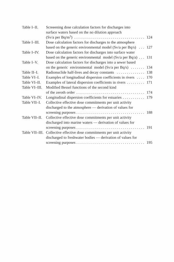
Table I–II. Screeening dose calculation factors for discharges intosurface waters based on the no dilution approach(Sv/a per Bq/m3) . . . . . . . . . . . . . . . . . . . . . . . . . . . . . . . . . . . 124

Table I–III. Dose calculation factors for discharges to the atmospherebased on the generic environmental model (Sv/a per Bq/s) . . . 127

Table I–IV. Dose calculation factors for discharges into surface water based on the generic environmental model (Sv/a per Bq/a) . . . 131

Table I–V. Dose calculation factors for discharges into a sewer basedon the generic environmental model (Sv/a per Bq/s) . . . . . . . 134

Table II–I. Radionuclide half-lives and decay constants . . . . . . . . . . . . . . 138Table VI–I. Examples of longitudinal dispersion coefficients in rivers . . . . 170Table VI–II. Examples of lateral dispersion coefficients in rivers . . . . . . . . . 171Table VI–III. Modified Bessel functions of the second kind

of the zeroth order . . . . . . . . . . . . . . . . . . . . . . . . . . . . . . . . . . 174Table VI–IV. Longitudinal dispersion coefficients for estuaries . . . . . . . . . . . 179Table VII–I. Collective effective dose commitments per unit activity

discharged to the atmosphere — derivation of values forscreening purposes . . . . . . . . . . . . . . . . . . . . . . . . . . . . . . . . . . 188

Table VII–II. Collective effective dose commitments per unit activitydischarged into marine waters — derivation of values forscreening purposes . . . . . . . . . . . . . . . . . . . . . . . . . . . . . . . . . . 191

Table VII–III. Collective effective dose commitments per unit activitydischarged to freshwater bodies — derivation of values forscreening purposes . . . . . . . . . . . . . . . . . . . . . . . . . . . . . . . . . . 195

1

1. INTRODUCTION

1.1. BACKGROUND

The International Basic Safety Standards for Protection against IonizingRadiation and for the Safety of Radiation Sources (BSS) [1] establish basic anddetailed requirements for protection against the risks associated with exposure toradiation and for the safety of radiation sources that may deliver such exposure. Thestandards are based primarily on the 1990 Recommendations of the InternationalCommission on Radiological Protection (ICRP) [2] and other IAEA Safety Seriespublications. The BSS [1] place requirements on both the Regulatory Authority andon the legal person responsible for a source. These requirements and the proceduresrequired to fulfill them are outlined in more detail in Ref. [3]. This Safety Reportsupports that publication and, in particular, provides the information necessary toallow the legal person responsible to “make an assessment of the nature, magnitudeand likelihood of the exposures attributed to the source” [1]. It provides a practicalgeneric methodology for assessing the impact of radionuclide discharges in terms ofthe resulting individual and collective radiation doses.

Previous guidance on models for predicting environmental transfer forassessing doses to the most exposed individuals (critical groups) was given in SafetySeries No. 57 [4]. Since the publication of that report, the IAEA has produced SafetySeries No. 100 on methods for evaluating the reliability of environmental transfermodel predictions [5]. A handbook of transfer data for the terrestrial and freshwaterenvironment [6] has also been produced which brings together relevant informationfrom the major data collections in the world. Many of the parameter values used inthis report are derived from the data in that handbook [6]. While Safety Series No. 57contained much useful information and has become, to some extent, a standard text,in practice it was incomplete since it did not include all the models that were neededfor assessment purposes. Moreover, considerable skill, expertise and resources wereneeded to derive and use appropriate data in the models.

This Safety Report expands on and supersedes the previous report [4]. Itincludes a new section on radiation dosimetry for intakes of radionuclides bymembers of the public and revised sections on atmospheric and aquatic dispersion. Asection on calculating collective doses for screening purposes is also included to helpdetermine whether further optimization procedures would be warranted. This SafetyReport is intended to be a complete and self-contained manual describing a simplebut robust assessment methodology that may be implemented without the need forspecial computing facilities.

1.2. OBJECTIVES

The main purpose of this Safety Report is to provide simple methods forcalculating doses1 arising from radioactive discharges into the environment, for thepurpose of evaluating suitable discharge limits and to allow comparison with therelevant dose limiting criteria specified by the relevant Regulatory Authority.

1.3. SCOPE

The models in this Safety Report have been developed for the purpose ofscreening proposed radioactive discharges (either from a new or existing practice);that is for determining through a simplified but conservative assessment the likelymagnitude of the impact, and whether it can be neglected from further considerationor whether more detailed analysis is necessary. The use of simple screening modelsfor dose assessment is one of the first steps in registering or licensing a practice, asexplained in more detail in Ref. [3]. A dose assessment will normally be requiredeither to demonstrate that the source may be exempted from the requirements of theBSS, or as part of the authorization or licence application. A step-wise procedure forsetting discharge limits is outlined in Ref. [3]. The function of the dose assessmentwithin this process, and the value of an iterative procedure in which the complexityof the dose assessment method increases as the magnitude of the predicted dosesincrease, is outlined in Ref. [3] and discussed in Sections 2 and 8 of this report.

This Safety Report provides the information required to assess rapidly dosesusing a minimum of site specific information. Two alternative methods are presented— a ‘no dilution’ approach that assumes members of the public are exposed at thepoint of discharge, and a generic environmental screening methodology that takesaccount of dilution and dispersion of discharges into the environment.

The screening models contained in this report are expected to be particularlyuseful for assessing the radiological impact of discharges from small scale facilities,for example hospitals or research laboratories. In these situations the development ofspecial local arrangements for dose assessment is likely to be unwarranted becausethe environmental discharges will usually be of a low level, and the methodologydescribed in this report will usually be adequate. However, for many larger scale

2

1 Unless otherwise stated, the term ‘dose’ refers to the sum of the effective dose fromexternal exposure in a given period and the committed effective dose from radionuclides takeninto the body in the same period.

nuclear facilities the assessed doses from the screening models presented in thisreport are more likely to approach the dose limiting criteria set by the RegulatoryAuthority (e.g. dose constraint), and users are more likely to need to follow ascreening calculation with a more realistic, site specific and detailed assessment.Such a re-evaluation may necessitate consultation with professionals in radiologicalassessment and the application of more advanced models. The description of theseadvanced models is outside the scope of this Safety Report.

Doses calculated using the screening models presented in this report do notrepresent actual doses received by particular individuals. Furthermore, it would notbe reasonable to use these models to reconstruct discharges from environmentalmonitoring measurements, because the pessimistic nature of the models might lead toa significant underestimation of the magnitude of the release.

The modelling approaches described in this report are applicable to continuousor prolonged releases into the environment when it is reasonable to assume that anequilibrium or quasi-equilibrium has been established with respect to the releasedradionuclides and the relevant components of the environment. The approachesdescribed here are not intended for application to instantaneous or short periodreleases such as might occur in uncontrolled or accident situations.

1.4. STRUCTURE

Section 2 provides an overview of the assessment methodology and discussesthe basic procedures for screening radionuclide discharges. The parameters andmodels for assessing the transfer between various environmental compartments forreleases of radionuclides to the atmosphere, into surface waters and to seweragesystems are described in Sections 3 to 5 of this report. Section 6 provides thenecessary dosimetric data and the equations by which individual doses may beevaluated. Section 7 considers collective doses, and Section 8 discusses theprocedures to be followed when calculated doses approach the relevant dose limitingcriteria.

In each section a simplified modelling procedure is described. Limitations inthe models and their use are discussed. Default values are provided for each of theparameters needed for the assessment — these are chosen from observed values insuch a manner as to produce only a small probability of underestimation of doses.

Annex I provides two types of dose calculation factors. The first, known as nodilution factors, allow rapid estimates to be made of the critical group doses arisingfrom a concentration in air or water (resulting from a discharge to the atmosphere ora river). These factors are intended to be used with the predicted maximumradionuclide concentrations at the point of discharge. This approach is likely tooverestimate significantly the doses received by members of the critical group in

3

reality. It is expected that these data will provide a useful screening method todetermine whether the discharge source may be automatically exempted from therequirements of the BSS (see Refs [1] and [3] for further discussion). Annex I alsoprovides generic dose calculation factors based on the generic environmental methodspresented in this report, and standardized assumptions regarding the dischargeconditions and the location of the critical group. These factors give the dose for a unitdischarge to the atmosphere or to a river or sewer. It is recommended that siteconditions should be taken into account in generic assessments if predicted dosesexceed a reference level, as explained in more detail in Section 2.

Radionuclide half-lives and decay constants are provided in Annex II, andspecial methods for calculating doses from 3H and 14C are described in Annex III.Annex IV provides a number of example calculations that illustrate the main featuresof the model.

Annexes V–VII provide more detailed information on some of the modelsincluded in this report. Annex V is a description of the Gaussian plume model,Annex VI covers the model for radionuclide transport in surface waters andAnnex VII gives an explanation of the methods used to assess collective doses.

A full listing of the parameter symbols used in the equations that describe themodel is provided at the end of the report. These symbols are listed, for ease ofreference, by the section in which they are used. A glossary of the terms used in thisSafety Report is also provided.

2. PROCEDURES FOR SCREENING RADIONUCLIDE DISCHARGES

2.1. DOSE CRITERIA AND CHOICE OF MODEL

An operation or practice that discharges radioactive materials into theenvironment is subject to evaluation according to the basic principles of radiationprotection. These principles are described in the BSS [1], and the specific issuesrelating to the control of discharges into the environment are described in a recentIAEA Safety Guide [3]. As indicated in Ref. [3], the calculation of critical groupdoses is a necessary component of the development of a discharge authorization. ThisSafety Report provides a simple screening approach for assessing critical group

4

doses2 and collective doses from discharges of radioactive substances into theenvironment.

Accurately assessing doses that could be received by members of the public canbe a complex and time consuming process. In many situations, where the doses likelyto be experienced by members of the public are very low and the expense ofundertaking a site specific assessment would not be warranted, it is possible to makesome simplifying and generally pessimistic assumptions that remove the necessity ofapplying complex modelling procedures or of gathering site specific data. This SafetyReport provides the information needed to perform such simplified assessments andrecommends a structured iterative approach for increasing the complexity ofmodelling as predicted doses approach or exceed a reference level which is related todose limiting criteria specified by the Regulatory Authority.

The first stage in the iterative approach recommended in this report is a verysimple assessment based on the conservative assumption that members of the publicare exposed at the point of discharge. This is referred to as the no dilution model.Dose calculation factors based on this approach are presented in Annex I of thisreport. As indicated in Fig. 1, it is recommended that a greater level of modelcomplexity would be necessary if the critical group dose predicted by the no dilutionmodel exceeds the relevant dose criterion (e.g. dose constraint). The second stage inthe iterative process is to use a simple generic environmental model that accounts forthe dispersion of radioactive materials in the environment. This model is explained insome detail in this Safety Report. Simple dose calculation factors, based on thisapproach, are also provided in Annex I. These factors are based on the genericenvironmental model and some standardized assumptions about discharge conditions,the location of food production and the habits and location of the critical group. Asindicated in Fig. 1, if predicted doses based on this generic environmental modelexceed a reference level, the next stage in the iterative assessment process is toexamine the generic input data for applicability to the site in question. If the data areoverly conservative or otherwise inapplicable, a modified generic assessment is calledfor. If the doses predicted using this approach also exceed the reference level it maybe necessary to consult a relevant expert to undertake a full site specific assessment.

2.1.1. Reference level

The choice of a value for the reference level to indicate when a greater level ofmodel complexity is needed warrants discussion. It is recommended that this level be

5

2 Dose criteria for members of the public are generally expressed in terms of the averagedose to the critical group. A critical group is representative of those members of the publiclikely to be most exposed (see the glossary).

6

FIG. 1. Iterative approach for assessing critical group doses.

Apply the no dilution approach

Is dose < dosecriterion?

Yes

Quality assuranceprocedures

End OK

NoApply the generic

environmental model

Is dose < referencelevel?

Yes

Quality assuranceprocedures

End OK

No

Check relevanceof generic

assumptions forsite

Apply modified genericassessment

Is dose < dosecriterion?

Yes

Quality assuranceprocedures

End OK

No

Apply the site specificmodel in consultationwith a suitable expert

specified to take account of both the relevant dose limiting criterion (e.g. the doseconstraint specified by the Regulatory Authority) and the level of uncertaintyassociated with the model predictions. In this context it is important to note that thegeneric environmental model and associated parameters presented in this report werederived such that

— Hypothetical critical group doses are generally likely to be overestimated,— Under no circumstances would doses be underestimated by more than a factor

of ten.

Thus it is fairly certain that doses experienced by the critical group will notexceed a particular dose criterion if the doses predicted using the generic model areless than one tenth of that criterion. This is consistent with the recommendation inRef. [3] that a reference level of 10% (or one tenth) of the dose constraint is areasonable basis for determining whether it is necessary to refine a dose assessment.The use of such a reference level to determine whether the no dilution approach issufficient would be overcautious in view of the extremely conservative nature of thisapproach. Comparison with the relevant dose criterion is therefore recommended asthe basis for deciding whether a more detailed assessment is necessary. A detaileddescription of the recommended iterative approach to be followed is given in Section 8.

2.2. GENERAL ASSESSMENT APPROACH

An overview of the assessment approach and the main parameters required tomake an assessment are given in Fig. 2. The first step in this approach is to estimatethe nature and magnitude of the proposed discharge of radioactive material into theenvironment, taking into account the period over which it is likely to occur. Transportof materials discharged to the atmosphere, surface water or a sewerage system ismodelled and the concentrations of radionuclides at locations where people may beexposed is assessed. Discharges to sewerage systems are assumed to result inexposure of workers at the sewage plant only. Projected doses arising from the otherdischarge routes are calculated at the point of discharge for the no dilution model, orat the closest locations where members of the public have access (e.g. for externaldose and inhalation dose calculations) or at the closest food production location (foringestion doses) for the generic environmental model. The assumed location, habitsand behaviour of members of the public are representative of those people likely tobe most exposed (the critical group).

The model is designed to estimate the maximum annual dose received duringthe period of the practice. The inventory of long lived radionuclides builds up in theenvironment, with the result that exposures may increase as the discharge continues.

7

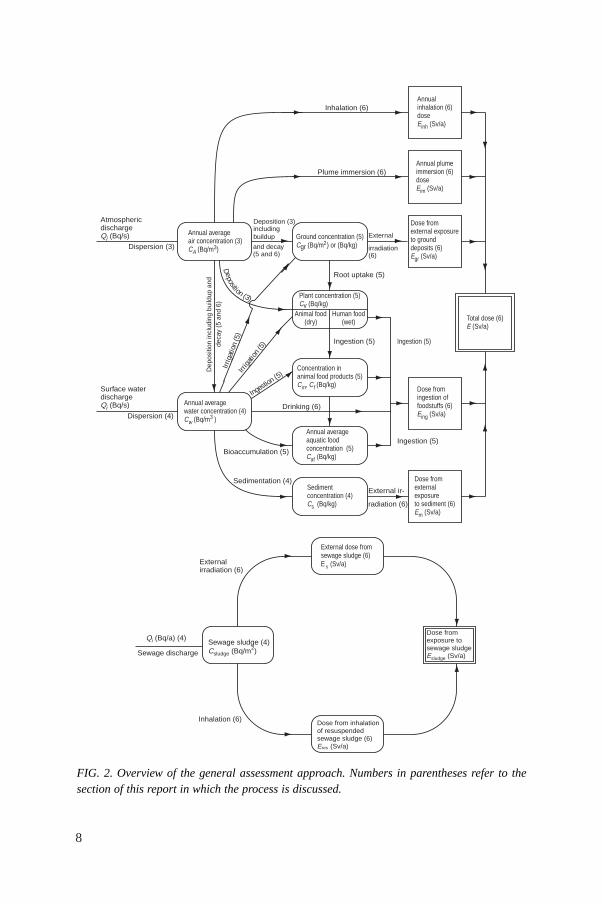
8

FIG. 2. Overview of the general assessment approach. Numbers in parentheses refer to thesection of this report in which the process is discussed.

Plant concentration (5)Cv (Bq/kg)

Ground concentration (5)Cgr (Bq/m ) or (Bq/kg)2

Annualinhalation (6)doseE (Sv/a)inh

Annual plumeimmersion (6)doseE (Sv/a)im

Dose fromexternal exposureto grounddeposits (6)E (Sv/a)gr

Dose fromingestion offoodstuffs (6)E (Sv/a)ing

Dose fromexternal exposureto sediment (6)E (Sv/a)m

Total dose (6) E (Sv/a)

Annual averageair concentration (3)C (Bq/m )A

3

Annual averagewater concentration (4)C (Bq/m )w

3

Concentration inanimal food products (5)C , C (Bq/kg)m f

Annual averageaquatic food concentration (5)C (Bq/kg)af

Sediment concentration (4)C (Bq/kg)s

Animal food(dry)

Human food(wet)

Inhalation (6)

AtmosphericdischargeQ (Bq/s)i

Dispersion (3)

Surface waterdischargeQ (Bq/s)i

Dispersion (4)Drinking (6)

Sedimentation (4)

Ingestion (5)

Ingestion (5)Ingestion (5)

Root uptake (5)

External ir-

radiation (6)

Bioaccumulation (5)

Irrig

atio

n (5

)

Deposition (3)

Irrig

ation

(5)

Ingestion (5)

deca

y (5

and

6)

Dep

ositi

on in

clud

ing

build

up a

nd

Plume immersion (6)

External

irradiation(6)

Deposition (3)includingbuildup

and decay (5 and 6)

External dose fromsewage sludge (6)E (Sv/a)s

Sewage sludge (4)C (Bq/m )sludge

2

Externalirradiation (6)

Inhalation (6)

Q (Bq/a) (4)

Sewage discharge

i

Dose from inhalationof resuspendedsewage sludge (6)E (Sv/a)res

Dose from exposure tosewage sludgeE (Sv/a)sludge

For generic model purposes the maximum annual dose is assumed to be the dose thatwould be received in the final year of the practice. A default discharge period of30 years is assumed, with the result that doses are estimated for the 30th year ofdischarge, and include the contribution to the dose from all material discharged in theprevious 29 years.

The exposure pathways considered, and the information needed to assess theircontributions to the dose, are illustrated in Fig. 2. External exposures from immersionin the plume and from material deposited on surfaces are included. Methods forassessing internal exposure, from the inhalation of radionuclides in the air and theingestion of radionuclides in food and water, are also provided. The recommendedapproach to account for exposures from multiple pathways is by simple summationover those pathways. In reality, it is unlikely that a member of the ‘true’ criticalgroup3 would be in the most exposed group for all exposure pathways. However, thesignificance of this potential compounding of pessimistic assumptions is somewhatlessened by the fact that the total dose is seldom dominated by more than a fewradionuclides and exposure pathways.

2.2.1. Estimation of the annual average discharge rate

In order to estimate the annual discharge rates for the screening models,information is required on the quantities and types of radionuclides to be discharged,the mode of discharge and the discharge points. In order to apply these models, thedischarge rate should be specified separately for the different release routes; that isfor discharges to the atmosphere (used as input in Section 3) and for discharges intosurface water or sewerage systems (used as input in Section 4).

The effects of any anticipated perturbations in the annual average discharge rateshould be taken into account. For example, it is recommended that operationalperturbations that are anticipated to occur with a frequency greater than 1 in 10 peryear should be included in the discharge rate estimate. In making this assessment careshould be taken to determine whether such perturbations are uniformly or randomlyspaced over the year. If they are dominated by a single event, a different doseassessment approach may be needed.

The inherent conservatism in the screening model is sufficient to accommodateuncertainties in the discharge rate if these uncertainties are no larger than a factor oftwo. Therefore a more realistic discharge rate estimate may be used in preference toa pessimistically derived one if the uncertainty in its value is less than about a factorof two.

9

3 In this context the true critical group is intended to represent those members of thepublic most exposed from a particular source, including contributions from all exposurepathways.

2.2.2. Estimation of environmental concentrations

2.2.2.1. Air and water

Once the discharge rate has been quantified, the next step in the procedure is toestimate the relevant annual average radionuclide concentration in air or water for thedischarge route of concern. If the no dispersion model is applied, the concentration atthe point of discharge is needed, while if the generic environmental model is appliedthe concentration at the location nearest to the facility at which a member of thepublic will be likely to have access, or from which a member of the public may obtainfood or water, is needed. The methods for estimating radionuclide concentrations inair are outlined in Section 3, while the approach for estimating concentrations insurface waters is outlined in Section 4. A screening model for estimating radionuclidetransport in sewerage systems and accumulation in sewage sludge is also described inSection 4.

The atmospheric dispersion model of the generic environmental model isdesigned to estimate annual average radionuclide concentrations in air and the annualaverage rate of deposition resulting from ground level and elevated sources of release.In locations where air flow patterns are influenced by the presence of large buildings,the model accounts for the effects of buildings on atmospheric dispersion ofradionuclides. The surface water model accounts for dispersion in rivers, small andlarge lakes, estuaries and along the coasts of oceans.

2.2.2.2. Terrestrial and aquatic foods

The methods for assessing radionuclide concentrations in terrestrial and aquaticfood products (assuming equilibrium conditions) are described in Section 5. Theaverage concentrations in terrestrial foods representative of the 30th year of operationmay be estimated from the annual average rate of deposition (Section 3), takingaccount of the buildup of radionuclides on surface soil over a 30 year period. Thetypes of terrestrial foods considered in Section 5 are milk, meat and vegetables. Theuptake and retention of radionuclides by terrestrial food products can take account ofdirect deposition from the atmosphere, and irrigation and uptake from soils. Theeffect of radionuclide intake through inadvertent soil ingestion by humans or grazinganimals is implicitly taken into account within the element specific values selected forthe soil to plant uptake coefficient.

The uptake and retention of radionuclides by aquatic biota is described inSection 5. The model uses selected element specific bioaccumulation factors thatdescribe an equilibrium state between the concentration of the radionuclide in biotaand water. The types of aquatic foods considered are freshwater fish, marine fish andmarine shellfish.

10

The use of surface water as a source of spray irrigation may be taken intoaccount by using the average concentration of the radionuclide in water, determinedfrom Section 4, and appropriate average irrigation rates, from Section 5, to estimatethe average deposition rate on to plant surfaces or agricultural land. Irrigation isassumed to occur for a period of 30 years. The contamination of surface water fromroutine discharges to the atmosphere is considered for both small and large lakes. Inthe case of a small lake, the estimate of direct deposition from the atmosphere ismodified by a term representing runoff from a contaminated watershed.

The process of radioactive decay is taken into account explicitly in the estimationof the retention of deposited radioactive materials on the surfaces of vegetation and onsoil, and in the estimation of the losses owing to decay that may occur during the timebetween harvest and human consumption of a given food item (Section 5).

2.2.3. Estimation of doses

As described in Section 6, calculated average radionuclide concentrations in air,food and water (representative of the 30th year of discharge) are combined with theannual rates of intake to obtain an estimate of the total radionuclide intake during thatyear. This total intake over the year is then multiplied by the appropriate dosecoefficient, given in Section 6, to obtain an estimate of the maximum effective dosein one year from inhalation or ingestion. In a similar manner, the concentrations ofradionuclides in shoreline sediments (Section 4) and surface soils (Section 5) in the30th year of discharge are used with appropriate dose coefficients to estimate theeffective dose received during that year from external irradiation.

The effective dose in one year from immersion in a cloud containingradionuclides may be calculated by multiplying the average concentration in air(Section 3) by the appropriate external dose coefficients in Section 6.

To obtain the total maximum effective dose in one year (representative of the30th year of discharge), the effective doses from all radionuclides and exposurepathways are summed. The equivalent dose estimates for the eyes and skin aresummed only for these tissues.

2.2.4. Screening estimates of collective dose

Section 7 provides tables of collective dose per unit activity discharged to theatmosphere and to the aquatic environment for a selection of radionuclides. These tablesmay be valuable for determining whether further optimization studies are worthwhile.These data are not intended for the purpose of rigorous site specific optimizationanalyses. The values provided in Section 7 are collective dose commitments, integratedto infinity. These data have uncertainties of the order of a factor of ten, and the data forvery long lived radionuclides represent very crude approximations.

11

3. ATMOSPHERIC DISPERSION

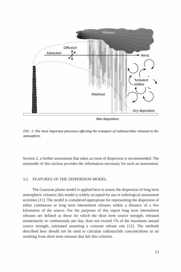
After release to the atmosphere, radionuclides undergo downwind transport(advection) and mixing processes (turbulent diffusion). Radioactive material will alsobe removed from the atmosphere by both wet and dry deposition on to the ground,and by radioactive decay. The most relevant mechanisms involved [7] are illustratedin Fig. 3. A model that takes account of these processes is needed to assessradionuclide concentrations at locations downwind of the release. This sectiondescribes a simple generic atmospheric dispersion model that allows for the aboveprocesses, and for the effects of any buildings in the vicinity of the release. Tables ofdispersion factors are provided to permit annual average radionuclide concentrationsin air, CA (Bq/m3), to be estimated on the basis of very limited site specific data.

Before describing this generic model, the relationship between radionuclideconcentration in air and the release in the absence of dispersion is given. Thisprovides the basis for the simple pessimistic no dilution approach described earlierand for the data presented in Annex I.

3.1. SCREENING CALCULATIONS

As indicated earlier, the simplest and most pessimistic screening technique is toassume that the radionuclide concentration at the point of interest (often referred toas the receptor location) is equal to the atmospheric radionuclide concentration at thepoint of release. Thus

(1)

where

CA is the ground level air concentration at downwind distance x (Bq/m3),Qi is the average discharge rate for radionuclide i (Bq/s),V is the volumetric air flow rate of the vent or stack at the point of release (m3/s),Pp is the fraction of the time the wind blows towards the receptor of interest

(dimensionless).

A value of Pp = 0.25 has been suggested for screening purposes [8–10]. Avalue of CA calculated using Eq. (1) can be used to calculate radionuclideconcentrations on the ground (Section 3.9) and subsequent doses to a member of thepublic located at the receptor point from other potential pathways of exposure (seeAnnex I). If the doses calculated in this way exceed a reference level, discussed in

CP Q

VAp i=

12

Section 2, a further assessment that takes account of dispersion is recommended. Theremainder of this section provides the information necessary for such an assessment.

3.2. FEATURES OF THE DISPERSION MODEL

The Gaussian plume model is applied here to assess the dispersion of long termatmospheric releases; this model is widely accepted for use in radiological assessmentactivities [11]. The model is considered appropriate for representing the dispersion ofeither continuous or long term intermittent releases within a distance of a fewkilometres of the source. For the purposes of this report long term intermittentreleases are defined as those for which the short term source strength, releasedmomentarily or continuously per day, does not exceed 1% of the maximum annualsource strength, estimated assuming a constant release rate [12]. The methodsdescribed here should not be used to calculate radionuclide concentrations in airresulting from short term releases that fail this criterion.

13

FIG. 3. The most important processes affecting the transport of radionuclides released to theatmosphere.

WindAdvection

Diffusion

Washout

Wet deposition

Dry deposition

Turbulenteddies

Rainout

A more detailed discussion of the Gaussian plume model and its limitations ispresented in Annex V. References [7, 11, 13, 14] provide a general overview of theuse of atmospheric dispersion models in radiological dose assessments. A moredetailed explanation of atmospheric transport phenomena is provided in the numerousscientific books and reports that have been published in this field, for example Refs[15–22].

3.3. BUILDING CONSIDERATIONS

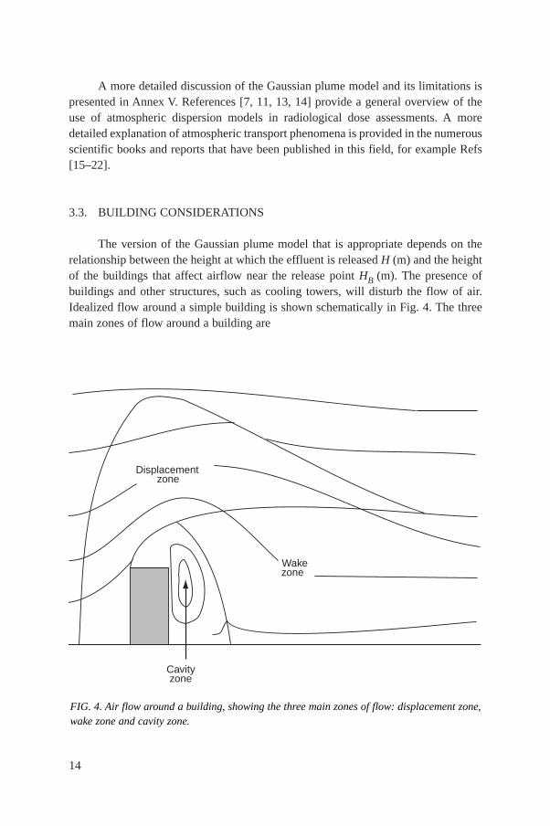
The version of the Gaussian plume model that is appropriate depends on therelationship between the height at which the effluent is released H (m) and the heightof the buildings that affect airflow near the release point HB (m). The presence ofbuildings and other structures, such as cooling towers, will disturb the flow of air.Idealized flow around a simple building is shown schematically in Fig. 4. The threemain zones of flow around a building are

14

FIG. 4. Air flow around a building, showing the three main zones of flow: displacement zone,wake zone and cavity zone.

Displacementzone

Wakezone

Cavityzone

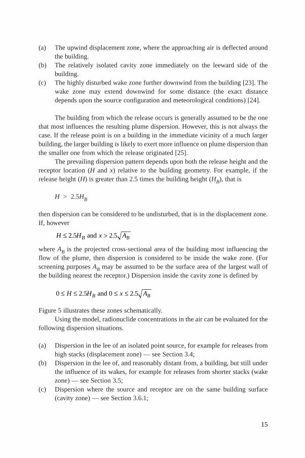
(a) The upwind displacement zone, where the approaching air is deflected aroundthe building.

(b) The relatively isolated cavity zone immediately on the leeward side of thebuilding.

(c) The highly disturbed wake zone further downwind from the building [23]. Thewake zone may extend downwind for some distance (the exact distancedepends upon the source configuration and meteorological conditions) [24].

The building from which the release occurs is generally assumed to be the onethat most influences the resulting plume dispersion. However, this is not always thecase. If the release point is on a building in the immediate vicinity of a much largerbuilding, the larger building is likely to exert more influence on plume dispersion thanthe smaller one from which the release originated [25].

The prevailing dispersion pattern depends upon both the release height and thereceptor location (H and x) relative to the building geometry. For example, if therelease height (H) is greater than 2.5 times the building height (HB), that is

H > 2.5HB

then dispersion can be considered to be undisturbed, that is in the displacement zone.If, however

where AB is the projected cross-sectional area of the building most influencing theflow of the plume, then dispersion is considered to be inside the wake zone. (Forscreening purposes AB may be assumed to be the surface area of the largest wall ofthe building nearest the receptor.) Dispersion inside the cavity zone is defined by

Figure 5 illustrates these zones schematically.Using the model, radionuclide concentrations in the air can be evaluated for the

following dispersion situations.

(a) Dispersion in the lee of an isolated point source, for example for releases fromhigh stacks (displacement zone) — see Section 3.4;

(b) Dispersion in the lee of, and reasonably distant from, a building, but still underthe influence of its wakes, for example for releases from shorter stacks (wakezone) — see Section 3.5;

(c) Dispersion where the source and receptor are on the same building surface(cavity zone) — see Section 3.6.1;

0 2 5 0 2 5£ £ £ £H H x AB B. .and

H H x AB B£ >2 5 2 5. .and

15

(d) Dispersion where the receptor is very close to, but not on, a building, forexample releases from a vent on a building (cavity zone) — see Section 3.6.2.

A flow chart showing the choice of appropriate dispersion conditions for thesescreening calculations is given in Fig. 6. For more detailed information on theseprocedures see Refs [24, 26, 27].

3.4. DISPERSION IN THE LEE OF AN ISOLATED POINT SOURCE,H > 2.5HB

The methods presented in this section are designed to be used for all cases thatdo not include building wake effects. This situation is depicted qualitatively in Fig. 7.The condition fulfilled is

H > 2.5HB

In this case the sector averaged form of the Gaussian plume model (see Annex V) maybe used with the following simplifying assumptions.

16

FIG. 5. Relationship between release height and receptor distance for determination of thetype of dispersion model to be used.

Receptor distance (x)

Dispersion in displacement zone(Section 3.4)

Dispersion inwake zone(Section 3.5)

Dispersion incavity zone(Section 3.6)

2.5 AB

2.5HB

Rel

ease

hei

ght (

H)

Building

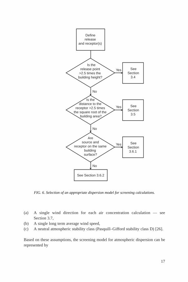
(a) A single wind direction for each air concentration calculation — seeSection 3.7,

(b) A single long term average wind speed,(c) A neutral atmospheric stability class (Pasquill–Gifford stability class D) [26].

Based on these assumptions, the screening model for atmospheric dispersion can berepresented by

17

FIG. 6. Selection of an appropriate dispersion model for screening calculations.

Definerelease

and receptor(s)

Is therelease point

>2.5 times thebuilding height?

Is thedistance to the

receptor >2.5 timesthe square root of the

building area?

Aresource and

receptor on the samebuildingsurface?

See Section 3.6.2

SeeSection

3.4

SeeSection

3.5

SeeSection3.6.1

Yes

No

No

No

Yes

Yes

(2)

where

CA is the ground level air concentration at downwind distance x in sector p (Bq/m3),Pp is the fraction of the time during the year that the wind blows towards the

receptor of interest in sector p,ua is the geometric mean of the wind speed at the height of release representative

of one year (m/s),F is the the Gaussian diffusion factor appropriate for the height of release H and

the downwind distance x being considered (m–2),Qi is the annual average discharge rate for radionuclide i (Bq/s).

Values of F as a function of downwind distance x for various values of H arepresented in Table I. These values were derived using the 30° sector averaged form ofthe Gaussian plume model; that is

(3)( )2 2

3

exp – /212×

2

z

z

HF

xp

È ˘Í ˙Î ˚=

σ

σ

CP FQ

uAp i

a

=

18

FIG. 7. Air flow in the displacement zone (H > 2.5HB). Building wake effects do not need tobe considered.

Receptorpoint

x

H

HB

where sz is the vertical diffusion parameter (m).These expressions are appropriate for dispersion over relatively flat terrain

without pronounced hills or valleys. The terrain is assumed to be covered withpastures, forests and small villages [27–31]. Three different expressions for thediffusion parameter were used in Eq. (3) to derive Table I. These assumptions arespecified in the notes to that table.

The general behaviour of the Gaussian plume model diffusion factor F as afunction of downwind distance for an elevated release is shown in Fig. 8. Forscreening purposes, however, it is assumed in this Safety Report that, for all H > 0,Fis constant between the point of release and the distance corresponding to themaximum value of F for that value of H — see the dashed line in Fig. 8. Thisapproach clearly overestimates the concentrations near the source, but it is considered

19

TABLE I. DISPERSION FACTOR (F, m–2) FOR NEUTRAL ATMOSPHERICSTRATIFICATION

Downwind Release height,H (m)distance,x (m) 0–5a 6–15a 16–25a 26–35a 36–45a 46–80b >80b

100 3 × 10–3 2 × 10–3 2 × 10–4 8 × 10–5 3 × 10–5 2 × 10–5 1 × 10–5

200 7 × 10–4 6 × 10–4 2 × 10–4 8 × 10–5 3 × 10–5 2 × 10–5 1 × 10–5

400 2 × 10–4 2 × 10–4 1 × 10–4 8 × 10–5 3 × 10–5 2 × 10–5 1 × 10–5

800 6 × 10–5 6 × 10–5 5 × 10–5 4 × 10–5 3 × 10–5 2 × 10–5 1 × 10–5

1 000 4 × 10–5 4 × 10–5 4 × 10–5 3 × 10–5 3 × 10–5 1 × 10–5 1 × 10–5

2 000 1 × 10–5 1 × 10–5 1 × 10–5 1 × 10–5 1 × 10–5 4 × 10–6 5 × 10–6

4 000 4 × 10–6 4 × 10–6 4 × 10–6 4 × 10–6 4 × 10–6 1 × 10–6 2 × 10–6

8 000 1 × 10–6 1 × 10–6 1 × 10–6 1 × 10–6 1 × 10–6 3 × 10–7 5 × 10–7

10 000 1 × 10–6 1 × 10–6 1 × 10–6 1 × 10–6 1 × 10–6 2 × 10–7 3 × 10–7

15 000 5 × 10–7 5 × 10–7 5 × 10–7 5 × 10–7 5 × 10–7 1 × 10–7 1 × 10–7

20 000 4 × 10–7 4 × 10–7 4 × 10–7 4 × 10–7 3 × 10–7 6 × 10–8 9 × 10–8

a Calculated on the basis of the following relationship [24]

b Calculated on the basis of the following relationship

sz = ExG

where E = 0.215 and G = 0.885 for release heights of 46–80 m, and E = 0.265 and G = 0.818

for release heights greater than 80 m [29–31].

(0.06)( ) / 1 (0.0015)( )z x xs = +

appropriate for screening purposes to ensure that actual doses are not underestimatedby more than a factor of ten.

3.5. DISPERSION IN THE LEE OF A BUILDING INSIDE THE WAKE ZONE

The methods described in this section are to be applied to all cases characterizedby the following criteria

Such a situation is shown qualitatively in Fig. 9. The concentration ofradionuclides in air is estimated using Eq. (2) corrected by a diffusion factorB (m–2)instead of F; that is

(4)CP BQ

uAp i

a=

H H x AB B£ >2 5 2 5. .and

20

FIG. 8. Relationship between the Gaussian plume diffusion factor (F) and the downwinddistance (x) for a given release height (H). In this screening approach, the maximum value ofF for a given value of H (indicated by the dashed line) is used for all distances less than orequal to the distance corresponding to the maximum value of F.

Downwind distance (x)

Screening assumption

Diff

usio

n fa

ctor

(F

)

where Pp, ua and Qi are as before (see Section 3.4) and

(5)

where

(6)

where

AB is the surface area of the appropriate wall of the building of concern (m2),sz is the vertical diffusion parameter (m) used in Eq. (3).

For long term dispersion, based on an assumed release height H = 0, the groundlevel activity concentration can be calculated by Eq. (4), see Refs [22] or [24]. Therespective numerical values of B for various cross-sectional areas of buildings are

 = +ÊËÁ

ˆ¯

≥z zB

BA

x Asp

20 5

2 5.

.for

Bx z

= ×∑

12

2

13π

21

FIG. 9. Air flow in the wake zone (H £ 2.5HB and x > 2.5 ).AB

Receptorpoint

x

H

HB

TABLE II. DISPERSION FACTOR WITH BUILDING WAKE CORRECTION (B, m–2) FOR NEUTRAL ATMOSPHERICSTRATIFICATION

Downwind Building surface area (m2)distance,x (m) 0–100 101–400 401–800 801–1200 1201–1600 1601–2000 2001–3000 3001–4000 4001–6000 >6000

100 3 × 10–3 2 × 10–3 1 × 10–3 9 × 10–4 8 × 10–4 7 × 10–4 6 × 10–4 5 × 10–4 4 × 10–4 3 × 10–4

200 7 × 10–4 6 × 10–4 5 × 10–4 4 × 10–4 3 × 10–4 3 × 10–4 3 × 10–4 2 × 10–4 2 × 10–4 2 × 10–4

400 2 × 10–4 2 × 10–4 2 × 10–4 2 × 10–4 1 × 10–4 1 × 10–4 1 × 10–4 1 × 10–4 9 × 10–5 8 × 10–5

800 6 × 10–5 6 × 10–5 6 × 10–5 5 × 10–5 5 × 10–5 5 × 10–5 5 × 10–5 4 × 10–5 4 × 10–5 4 × 10–5

1 000 4 × 10–5 4 × 10–5 4 × 10–5 4 × 10–5 4 × 10–5 3 × 10–5 3 × 10–5 3 × 10–5 3 × 10–5 3 × 10–5

2 000 1 × 10–5 1 × 10–5 1 × 10–5 1 × 10–5 1 × 10–5 1 × 10–5 1 × 10–5 1 × 10–5 1 × 10–5 1 × 10–5

4 000 4 × 10–6 4 × 10–6 4 × 10–6 4 × 10–6 4 × 10–6 4 × 10–6 4 × 10–6 4 × 10–6 4 × 10–6 4 × 10–6

8 000 1 × 10–6 1 × 10–6 1 × 10–6 1 × 10–6 1 × 10–6 1 × 10–6 1 × 10–6 1 × 10–6 1 × 10–6 1 × 10–6

10 000 1 × 10–6 1 × 10–6 1 × 10–6 1 × 10–6 1 × 10–6 1 × 10–6 1 × 10–6 1 × 10–6 1 × 10–6 1 × 10–6

15 000 5 × 10–7 5 × 10–7 5 × 10–7 5 × 10–7 5 × 10–7 5 × 10–7 5 × 10–7 5 × 10–7 5 × 10–7 5 × 10–7

20 000 4 × 10–7 4 × 10–7 4 × 10–7 4 × 10–7 4 × 10–7 4 × 10–7 4 × 10–7 4 × 10–7 4 × 10–7 4 × 10–7

22

shown in Table II. These values represent reasonable estimates of turbulent mixing forground level releases (H = 0) only. Application to elevated releases results in rathercrude and pessimistic estimates of the dispersion situation, which are neverthelessappropriate for screening purposes.

3.6. DISPERSION IN THE LEE OF A BUILDING INSIDE THE CAVITY ZONE

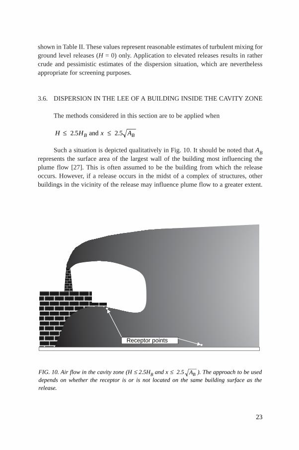
The methods considered in this section are to be applied when

Such a situation is depicted qualitatively in Fig. 10. It should be noted that ABrepresents the surface area of the largest wall of the building most influencing theplume flow [27]. This is often assumed to be the building from which the releaseoccurs. However, if a release occurs in the midst of a complex of structures, otherbuildings in the vicinity of the release may influence plume flow to a greater extent.

H H x AB B£ £2 5 2 5. .and

23

FIG. 10. Air flow in the cavity zone (H £ 2.5HB and x £ 2.5 ). The approach to be useddepends on whether the receptor is or is not located on the same building surface as therelease.

AB

Receptor points

It is important to ensure that the correct building is considered when calculationsusing these procedures are made [25].

3.6.1. Source and receptor on same building surface

This case represents the situation where the receptor point or person of interestis on the same building surface, for example a roof or side wall opening such as awindow, or in the building from which the release occurs. To predict the maximumconcentration expected at a receptor locatedx metres from the release point, thefollowing procedure has been adapted from information given in Ref. [27].

(a) If x is less than or equal to three times the diameter of the stack or vent fromwhich the radionuclide is emitted, it may be assumed that no dilution occurs inthe atmosphere and, as a result, the air concentration at the receptor point isequal to the concentration of the radionuclide at the point of release (as givenin Eq. (1)).

(b) If x is greater than three times the diameter of the stack or vent, use Eq. (7)below to calculate the air concentration with B0 = 30

(7)

The unitless constant B0 accounts for potential increases in the concentration inair along a vertical wall owing to the presence of zones of air stagnation created bybuilding wakes.

3.6.2. Source and receptor not on same building surface

For this situation the following equation is used to calculate the radionuclideconcentration in air [32]

(8)

where K is a constant of value 1 m. This model is an empirical formulation thatyielded conservative predicted concentrations in air when compared with about40 sets of field data from tracer experiments around nuclear reactor structures. If thewidth of the building under consideration is less than its height, the width of thebuilding should be used in place of HB in Eq. (8) [33].

CP Q

u H KAp i

a B=

p

CB Q

u xA

i

a

= 02

24

3.7. DEFAULT INPUT DATA

The generic approach described above has been designed to require a minimuminput of data by the user. The radionuclide discharge rate and the location of therelease point and the receptor (i.e. Qi, H, HB, AB and x), however, must be specifiedfor the particular situation considered. No default values can be given for theseparameters, although standardized assumptions have been applied to derive thegeneric dose calculation factors given in Annex I. The user is cautioned that theseparameters should be determined as accurately as possible. The value of H usedshould ideally include both the physical height of the release point and any additionalheight resulting from the rise of the effluent plume owing to thermal or mechanicaleffects [28]. However, neglecting plume rise will tend to result in an overpredictionof downwind air concentrations and, therefore, is appropriate for a genericassessment.

The building surface area used,AB, should be that of the building mostinfluencing the air flow around the source [27]. For most releases this will be thebuilding from which the release occurs. If the release point is surrounded by otherbuildings and similar structures, such as cooling towers, a building other than the oneassociated with the release may need to be used for AB. The downwind distance x usedin the screening calculations should be the location of the nearest point of interest fordose calculation purposes. This location may be different for different pathways ofexposure. For example, the nearest point of public access to a facility would beappropriate for the inhalation and external exposure pathways, while the nearestlocation where food could be grown would be appropriate for assessing doses fromterrestrial food pathways. This may result in multiple air concentrations beingrequired for a single facility assessment. It should also be noted that the Gaussianplume model is not generally applicable at x > 20 km. As a result, it is recommendedthat any receptors of concern that are beyond 20 km from the release point shouldbe considered to be at x = 20 km for generic assessment purposes. In using Tables Iand II, if x falls between two values given in the table the smaller distance shouldbe used.

The only meteorological variables required arePp and ua. For detailed longterm radiological dose assessments the frequency with which the wind blows ineach of 12 cardinal wind directions may be obtained from local climatologicalinformation. (The sum of the frequencies for all directions is automatically equalto 1.) For generic assessment purposes, however, only one wind direction isconsidered for each individual air concentration calculation. To help reduce thechance of the predicted values being more than a factor of ten lower than theactual doses, it should be assumed thatPp = 0.25 for this single direction. It ispreferable to use a site specific value for the wind speed ua at the height of therelease, determined either by measurement or by extrapolation [7]. In the event

25

that information onua appropriate for the release location is not readily available,however, it is suggested that a default value of ua = 2 m/s be used [8–10].

3.8. PLUME DEPLETION

As noted earlier, and in Fig. 3, a plume of radioactive material may be depletedas it moves downwind. Removal processes include [7]

— Radioactive decay,— Plume depletion by dry deposition,— Plume depletion by precipitation scavenging (wet deposition).

Over the relatively short distances of a few kilometres considered here,corrections of the plume activity owing to wet and/or dry deposition can usually beneglected when calculating the annual average concentrations of radionuclides in air.In any case, when plume depletion is not incorporated into the assessment, the resultwill be conservative.

Depletion of the activity in the plume owing to radioactive decay can also beneglected for most of the radionuclides. This is particularly true if discharges occurafter initial retention of short lived radionuclides. Thus radioactive decay may beneglected, except for very short lived nuclides. Where radioactive decay is likely tobe significant, calculated air concentrations can be modified by multiplying by areduction factor f where

(9)

and li is the radioactive decay constant of radionuclide i (s–1). Values for li areprovided in Annex II.

3.9. GROUND DEPOSITION

Activity concentrations of radionuclides on the ground can be calculated simplyby using ratios representing the amount of activity deposited on the ground per unittime and the ground level air concentration. These ratios are called depositionvelocities or, better, deposition coefficients, because their physical meaning is not thatof a velocity. Further information on wet and dry deposition coefficients is given inRefs [13, 15, 18, 21, 34, 35].

For generic assessment purposes the following relationship is used

fx

uia

= −

exp λ

26

d·i = (Vd + Vw) CA

(10)

where

d·i is the total daily average deposition rate on the ground of a given radionuclide

i from both dry and wet processes, including deposition either on toimpervious surfaces or on to both vegetation and soil (Bq◊m–2◊d–1);

Vd is the dry deposition coefficient for a given radionuclide (m/d);Vw is the wet deposition coefficient for a given radionuclide (m/d).

As indicated in Section 5, the deposition rate d·i is used to calculate the radio-

nuclide concentration on vegetation owing to direct contamination (Cv,i,1 in Eq. (30)) andthe concentration of radionuclide in dry soil (Cs,i in Eq. (32) or Cgr in Eq. (42)).

Measured values of Vd and Vw for radionuclides are quite variable. They dependon such factors as the physical and chemical form of the radionuclide, the nature ofthe depositing surface, meteorological conditions and, in the case of Vw, theprecipitation rate [25]. It has been recommended that a total deposition coefficient,VT(= Vd + Vw), of 1000 m/d be used for screening purposes for deposition of aerosolsand reactive gases [8–10]. This value of VT is consistent with values for 131I and 137Csfallout resulting from the accident at the Chernobyl nuclear power station in 1986[36]. It should be noted, however, that the Chernobyl fallout aerosols were well mixedin the atmosphere by the time the measurements were taken. Materials deposited nearthe point of release are likely to be less well mixed. As a result, it is expected thatusing VT = 1000 m/d will result in a conservative estimate of total deposition forscreening purposes [25]. For 3H, 14C and non-reactive gases such as krypton it shouldbe assumed thatVT = 0 [7–10].

Deposition from a plume of material in the atmosphere may result not only inradionuclides on the ground but also in lakes in the vicinity of the release. This mayoccur by both direct deposition on to the lake surface and from runoff into the lake ofmaterial initially deposited on the land surface. As noted earlier, Gaussian plumeprocedures for calculating air concentrations are designed to be used within 20 km ofthe release point. If a lake is found within this radius, it is recommended that thedeposition rate at the centre of the lake should be calculated, and the methodspresented in Section 4 may be used to estimate the resulting water concentration.

3.10. RESUSPENSION OF DEPOSITED RADIONUCLIDES

Radionuclides on the ground can be resuspended into the air by the action ofwind and other disturbances. There have been several reviews of the processesinvolved (see, for example, Refs [37, 38]). Resuspension mechanisms can be broadly

27

divided into human-made and wind driven disturbances. Resuspension caused byhuman-made disturbances, such as vehicular traffic, digging and farming activities, isusually localized and of potential importance only for the exposure of a fewindividuals. Wind driven resuspension leads to more general exposure. Resuspensionhas been included in previous generic calculations, for example in Ref. [4]. However,it is generally found to be a relatively minor exposure pathway following routinedischarges of radionuclides to the atmosphere [39]. It is relatively important onlywhere there is no continuing discharge and, for those radionuclides such as theactinides, where doses owing to external irradiation and food chain transfer arerelatively unimportant. Resuspension is therefore not considered further here.Appropriate models are described in Ref. [39]. This pathway is, however, taken intoaccount when assessing doses to workers exposed to sewage sludge, as described inSection 4.

3.11. ESTIMATES FOR AREA SOURCES

The models presented in this section are designed for use with releases frompoint sources, not area or volume sources such as from uranium mill tailings. It hasbeen suggested, however, that the following procedures could be used to calculate theconcentration in air from an area source [25].

(a) Calculate a pseudo point source release rate by integrating over the entire areaof the source,

(b) Assume the release height to be zero,(c) Locate the release point at the edge of the area source nearest the location of

concern.

Use of this procedure should result in a conservative estimate of the concentration in air.

3.12. UNCERTAINTY ASSOCIATED WITH THESE PROCEDURES

As indicated earlier, the methodology presented in this Safety Report isdesigned to minimize the possibility that the calculated doses will underestimate realdoses by more than a factor of ten. The concepts presented in this section forcalculating the radionuclide concentrations in air are based primarily onrecommendations for models presented elsewhere [7–10]. The procedures outlined inone of these reports [8] have been carefully evaluated to determine the degree ofconservatism that they represent [25]. The results of that review may be summarizedas follows.

28

29

(a) For isolated point sources the Gaussian plume model appears to be capable ofpredicting long term average air concentrations within a factor of four for flatterrain and within a factor of ten for sites with complex terrain and meteorology[40].

(b) For releases near buildings and receptors within a distance equal to 2.5 timesthe square root of the building frontal area the models presented are generallyconservative. However, these models should not be used in situations whereconfinement of the plume is probable, for example for releases into a streetcanyon.

(c) For releases near buildings and receptors at distances larger than 2.5 times thesquare root of the building frontal area predicted concentrations are expected tobe within a factor of two for simple building shapes and flat terrain. However,the model presented here begins to underpredict consistently for wind speedsgreater than 5 m/s [41].

(d) The default assumptions of Pp = 0.25,ua = 2 m/s,VT = 1000 m/d, plume rise = 0and plume depletion = 0 are believed to be conservative in nature.

(e) The bias is unknown for the assumption that class D atmospheric stabilityprevails 100% of the time.

4. RADIONUCLIDE TRANSPORT IN SURFACE WATERS

This section describes generic methods for estimating radionuclideconcentrations in water,Cw (Bq/m3), and in sediment,Cs (Bq/kg), from routine radio-nuclide discharges into surface water,Qi (Bq/s) (Fig. 2). The following types ofsurface water are considered.

— Rivers,— Estuaries,— Coastal waters,— Small lakes,— Large lakes.

Radionuclides discharged into surface waters are subject to a series of physicaland chemical processes that affect their transport from the source point. Theseprocesses include

— Flow processes, such as downcurrent transport (advection) and mixingprocesses (turbulent dispersion);

— Sediment processes, such as adsorption/desorption on suspended, shore/beachand bottom sediments, and downcurrent transport, deposition and resuspensionof sediment, which adsorbs radionuclides;

— Other processes, including radionuclide decay and other mechanisms that willreduce concentrations in water, such as radionuclide volatilization (if any).

These processes are illustrated in Fig. 11 and are described in more detail inRefs [42, 43]. The processes are, in general, three dimensional and transient in nature.However, a generic assessment of annual average radionuclide concentrations fromroutine discharges can be made on the assumption that a number of processes are ata steady state.

Before describing the generic approach applied to each surface water body, therelationship between the discharge rate and the radionuclide concentration in water isprovided for the screening assumption that all water usage occurs at the point ofrelease. Features of the generic modelling procedure that are common to all surfacewater types are then outlined, followed by the generic model for each of the surfacewater types in turn. Uncertainty issues are discussed before finally describing amodelling approach for assessing discharges to a sewerage system.

4.1. SCREENING CALCULATIONS

As in Section 2, the simplest and most pessimistic approach for screeningpurposes is to neglect dilution effects — that is in effect to assume that exposure occursat the point of discharge. This approach is independent of the type of water body intowhich the discharge occurs. The concentration in water under these circumstances isgiven by

(11)

where

Cw, tot is the total radionuclide concentration (Bq/m3),C0 is the radionuclide concentration in the effluent discharge outfall (Bq/m3),Qi is the annual average discharge rate for radionuclide i (Bq/s),F is the flow rate of the liquid effluent (m3/s).

A value of Cw, tot calculated using Eq. (11) can be used to calculate radionuclideconcentrations in sediment and aquatic foods and subsequent critical group doses (seeAnnex I). As indicated in Section 2, if the doses calculated in this way exceed therelevant dose criterion, a further assessment that takes account of dilution in the

C CQ

Fwi

, tot = =0

30

31

FIG. 11. Processes affecting the movement of radionuclides from the point of discharge into a river.

River flow

River bank

Mixing Sorptionby suspendedand bottom

sediment

Radionuclidereduction

by decay andsedimentation

Absorption by shore sediment

appropriate surface water body (i.e. river, estuary, coastal water, small lake or largelake) is recommended. The remainder of Section 4 provides the information necessaryfor such assessments.

4.2. FEATURES OF MODELS OF DILUTION IN SURFACE WATERS

There are three basic types of model used to estimate radionuclide transport insurface waters [44].

— Numerical models usually transform basic equations describing radionuclidedispersion into finite difference or finite element forms.

— Box type models treat the entire water body or sections of a water body ashomogeneous compartments. These models often include some sediment–radio-nuclide interactions.

— Analytical models solve the basic radionuclide transport equations. Simplifyingassumptions are made regarding water body geometry, flow conditions and disper-sion processes in order to obtain analytical solutions to the governing equations.

The generic methodology presented in this Safety Report is based on analyticalsolutions to advection–diffusion equations describing radionuclide transport insurface waters with steady state uniform flow conditions. A box type model has beenused for small lakes and reservoirs. The detailed derivation of these solutions andassociated assumptions is discussed in Annex VI.

Radionuclide concentrations in water (and sediment) may be calculated forspecific locations where members of hypothetical critical groups could use this waterfor drinking, fishing, irrigation or swimming, and could use the sediment forrecreational or agricultural activities. These locations (at a specified distance x fromthe point of discharge) are selected to represent the nearest point where water usageis conceivable during the projected lifetime of an operating facility. The methodologyalso includes simple processes to estimate default dispersion coefficients, river flowconditions and the coastal current, if site specific values are unavailable.

If there is more than one source of radionuclide discharge, it is recommendedthat the radionuclide concentration for each of the discharges be calculated separately.The cumulative radionuclide concentration at location x may then be obtained bysumming the results for the individual radionuclides.

4.2.1. Sediment effects

Radionuclides may become adsorbed on to sediments in water, thus reducingthe dissolved radionuclide concentration in the water column. However, radionuclides

32

adsorbed on to suspended sediment may still migrate downstream, deposit to theriver/sea bottom and then be resuspended from the bottom and become incorporatedin banks and beaches [45]. These processes are highly site specific. Over a period oftime, remobilization of radionuclides associated with deposited sediments maybecome an additional source of exposure to members of critical population groups,the importance of which depends upon the radionuclide involved.

It is possible to calculate radionuclide concentrations in sediment, corres-ponding to the concentration in water, by using a distribution coefficient Kd (L/kg).However, it is recommended that the effect of sediment adsorption be ignored, for thesake of simplicity, for screening purposes and because this approach will tend tooverestimate radionuclide concentrations in water and doses from direct uses of water(e.g. drinking). This approach is followed here, although data required to take accountof sediment effects are presented in Section 4.7.

4.2.2. Applicability and limitations of the models

As a result of the simplifying assumptions implicit in its derivation, this genericmethodology strictly applies only if the following conditions are satisfied.

(a) The surface water geometry (e.g. river cross-section, shoreline) does not changegreatly with distance;

(b) The flow characteristics (e.g. flow velocity, water depth) do not change signifi-cantly with distance or with time;

(c) Radionuclides in water and sediment, under the conditions of a routine, longterm release, can be considered to be in equilibrium.

This approach is often used to assess the distribution of contaminants in surfacewaters [44, 46–48]. Annex VI provides more details and general solutions to theequations describing radionuclide transport.

4.2.2.1. Conservatism

A degree of conservatism (i.e. the tendency to overestimate actual concentra-tions) is necessary for such a generic approach, and in this methodology this isderived from the following conditions.

(1) The locations where surface waters or sediments are assumed to be utilized byhypothetical critical group members are intentionally selected to limit thepotential for underestimating actual exposures.

(2) Values for flow rates, current velocity and water depth are representative of thelowest annual average conditions occurring over a period of 30 years.

33

34

(3) Radionuclide concentrations are calculated along the plume centreline (exceptfor concentrations along a coastal shoreline).

(4) Radionuclides are assumed to be released along the bank of a river, estuary orlarge lake, thus restricting mixing.

(5) Additional conservatism can be achieved by excluding the effect of sedimentadsorption (thus maximizing the estimate of the concentrations of radionuclidesin the water for estimation of doses resulting from the direct use of the water).

4.3. RIVERS

The model has been developed to allow the radionuclide concentration in waterto be calculated at a location along either the river bank from which the dischargeoccurs or along the opposite bank (see Fig. 11). It has been designed to require aminimum input of site specific data. As indicated above, an initial estimate of theradionuclide concentration in water can be made by neglecting sediment effects.However, the approach needed to take account of the effects of water filtration andsedimentation is described in Section 4.7.

4.3.1. Basic river characteristics required for calculations

The following three parameters are required to calculate radionuclideconcentrations in a river (corresponding to the lowest annual river flow rates expectedin a 30 year period).

(a) River width B (m),(b) Longitudinal distance from the release point to a potential receptor location x (m),(c) Radionuclide decay constant li (s–1).

Site specific values for the following are desirable: 30 year low annual riverflow rate qr (m3/s); flow depth D (m), that corresponds to qr ; river velocity U (m/s),that corresponds to qr .

If such data are not available, they may be estimated, on the basis ofhydrological studies [49], as indicated in Section 4.3.1.1.

The longitudinal distance for complete mixing is based on the assumption thatcomplete lateral and vertical mixing is achieved when the minimum concentration isone half of the maximum concentration along the same lateral and vertical lines. Thelongitudinal distance required to achieve this vertical complete mixing, Lz (m), is

Lz = 7D

4.3.1.1. Estimating a default value for the river flow rate

From observation or a map estimate a river width B–

(m) under normal river flowconditions upstream of the estuary, where there is no tidal effect on the river flow.

The mean annual river flow rate q–

r (m3/s) that corresponds to the river width B–

may be obtained from Table III. For default purposes it may be assumed that the30 year low annual river flow rate qr (m3/s) is 1/3 of the mean annual river flow rateq–

r. The river width B (m) and depthD (m) that corresponds to the 30 year low annualriver flow rate qr (m3/s) may then be obtained from Table III.

The net freshwater velocity U (m/s) corresponding to the 30 year low annualriver flow rate may be calculated by taking

4.3.2. Calculation of radionuclide concentrations

The procedure for calculating radionuclide concentrations is illustrated in theform of a flow chart in Fig. 12. Two situations are considered below.

4.3.2.1. Water usage on the river bank opposite to the radionuclide discharge point

In this case a radionuclide must traverse at least half of the river width to reachthe bank opposite to the discharge point, and the maximum radionuclide concentrationis the cross-sectionally averaged concentration. Thus the radionuclide concentrationin unfiltered water at the opposite bank can be obtained by

(12)

where

Cw, tot is the total radionuclide concentration in water (Bq/m3),Qi is the average discharge rate for radionuclide i (Bq/s),qr is the mean river flow rate (m3/s),li is the radioactive decay constant (s–1),x is the distance between the discharge point and the receptor (m),U is the net freshwater velocity (m/s).

Values for radionuclide decay constants (li) are provided in Annex II.

CQ

q

x

UCw

i

r

it, exptot = −

=λ

Uq

BDr=

35

4.3.2.2. Water usage on the same river bank as the radionuclide discharge point

If water usage occurs on the same bank as the discharge, and at a locationbefore complete vertical mixing can occur (i.e. x £ Lz = 7D), the radionuclideconcentration in water may be assumed to be undiluted; that is it is assumed to be the

36

0.10.20.30.40.50.60.70.80.9123456789

102030405060708090

3.474.775.756.567.277.918.499.029.53

10.013.816.618.921.022.824.526.027.528.839.747.854.660.565.870.675.179.2

0.0580.0790.0950.1080.1200.1300.1390.1480.1560.160.220.270.300.340.360.390.410.440.480.630.750.850.941.021.091.161.22

100200300400500600700800900

1 0002 0003 0004 0005 0006 0007 0008 0009 000

10 00020 00030 00040 00050 00060 00070 00080 00090 000

100 000

83.2114138157174190204216229240330398454503547587624659692952

1 1501 3101 4501 5801 6901 8001 9002 000

1.281.742.092.372.622.843.053.243.413.574.875.846.647.347.968.539.059.5410.013.616.318.620.522.323.925.326.728.0

TABLE III. RELATIONSHIPS BETWEEN RIVER FLOW RATE, RIVER WIDTHAND DEPTHa

a Using linear interpolation between values.

River flowrate,qr(m3/s)

River width,B

(m)

Depth,D

(m)

River flowrate,qr(m3/s)

River width,B

(m)

Depth,D

(m)

37

FIG. 12. Procedure for calculating radionuclide concentrations in water resulting from adischarge into a river.

qr

3

qr

BD

1.5Dx

B2

Use six steps: Estimate B Get q from Table III

Calculate q =

Get B from Table IIIGet D from Table III

Calculate U =

••

•

••

•

r

r

Select x

Do you know low river flow conditions? (q U, B, D) r

No

Yes

Is on the same

bank side?

x

Yes

No x > 7D?

Yes

•

•

Calculate A =

Obtain P from Table IVr

No

C = C0 qrPrU

Qili x

C = exp( )–qrPrU

Qili x

C = exp( )–

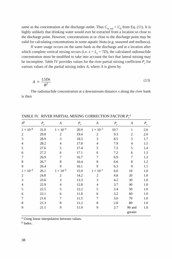
same as the concentration at the discharge outlet. Thus Cw, tot = C0 from Eq. (11). It ishighly unlikely that drinking water would ever be extracted from a location so close tothe discharge point. However, concentrations at or close to the discharge point may bevalid for calculating concentrations in some aquatic biota (e.g. seaweed and mollusca).

If water usage occurs on the same bank as the discharge and at a location afterwhich complete vertical mixing occurs (i.e. x > Lz = 7D), the calculated radionuclideconcentration must be modified to take into account the fact that lateral mixing maybe incomplete. Table IV provides values for the river partial mixing coefficient Pr forvarious values of the partial mixing index A, where A is given by

(13)

The radionuclide concentration at a downstream distancex along the river bankis then

ADx

B= 15

2

.

38

TABLE IV. RIVER PARTIAL MIXING CORRECTION FACTOR Pra

Ab Pr A Pr A Pr A Pr

1 × 10–6 31.0 1 × 10–4 20.9 1 × 10–2 10.7 1 2.62 29.8 2 19.4 2 9.3 2 2.03 28.9 3 18.5 3 8.5 3 1.74 28.2 4 17.8 4 7.9 4 1.55 27.6 5 17.4 5 7.5 5 1.46 27.2 6 17.1 6 7.2 6 1.37 26.9 7 16.7 7 6.9 7 1.38 26.7 8 16.4 8 6.6 8 1.29 26.4 9 16.1 9 6.3 9 1.11 × 10–5 26.1 1 × 10–3 15.9 1 × 10–1 6.0 10 1.02 24.8 2 14.2 2 4.8 20 1.03 23.6 3 13.3 3 4.2 30 1.04 22.9 4 12.8 4 3.7 40 1.05 22.5 5 12.2 5 3.4 50 1.06 22.1 6 11.8 6 3.2 60 1.07 21.6 7 11.5 7 3.0 70 1.08 21.3 8 11.2 8 2.8 80 1.09 21.1 9 11.0 9 2.7 90 and 1.0

greater

a Using linear interpolation between values.b Index.

Cw, tot = Ct Pr (14)

Note that the fully mixed radionuclide concentration Ct is given by Eq. (12).The variable Pr can be regarded as a correction factor for the partial mixing, and

it approaches unity as the downstream distance x increases. (Note that for x > 3 B2/D,Pr ª 1, as discussed in Annex VI.)

4.4. ESTUARIES

4.4.1. Estuarine regions

An estuary is a water body that is connected at one end to a river and at the otherend to the sea. An estuary velocity reverses with the tide, and an estuary can containfresh or saline water, although it is generally less saline than that of the sea. For thepurposes of this generic methodology a radioactive discharge is assumed to occurfrom one of the estuarine banks. The radionuclide concentration at the banks may beassessed using a methodology that is very similar to that for rivers, but with someadjustments to account for tidal effects. (See Annex VI for a detailed description ofthe estuarine methodology.)

4.4.2. Basic estuarine characteristics required for calculation

The following variables and parameters are required to calculate theradionuclide concentration in an estuary: estuarine width B (m); estuarine flow depthD (m); river width B

–(m) under a mean annual river flow rate upstream of the tidal

flow area tidal period Tp (s); longitudinal distance from the release point to a potentialreceptor location x (m); and radionuclide decay constant li (s–1).

The longitudinal distances at which complete vertical mixing is achieved isassumed to occur when the minimum concentration is at least half of the maximumconcentration along the vertical direction. The longitudinal distance required toachieve this complete vertical mixing Lz (m) is

Lz = 7D

The radionuclide upstream travel distance Lu (m) is calculated by

Lu = 0.32ΩUfΩTp (15)

39

40

4.4.2.1. Estimating a default value for the river flow rate and tidal velocities

From observation or a map the river width B–

(m) under normal river flowconditions upstream of the estuary, where there is no tidal effect on the river flow,may be estimated.

The mean river flow rate q–

r (m3/s) that corresponds to the river width B–

may beobtained from Table III. For default purposes it may be assumed that the 30 year lowannual river flow rate q

–r (m3/s) is 1/3 of the mean annual river flow rate qr. The net

freshwater velocity U (m/s) corresponding to the 30 year low annual river flow ratemay be calculated by taking

If the maximum ebb (seaward) velocity Ue (m/s) and the flood (upstream)velocity Uf (m/s) is not available, it is possible to assume

Ue = 0.5 m/sUf = 0.5 m/s

The mean tidal flow speed Ut and the tidal flow rate qw may then be estimatedby taking

Ut = 0.32(ΩUeΩ+ΩUfΩ), qw = DBUt

4.4.3. Calculation of radionuclide concentrations

The procedure for calculating radionuclide concentrations in water at a locationalong the banks of an estuary is illustrated in the form of a flow chart in Fig. 13. Foursituations are considered as described.

4.4.3.1. Water usage on the bank of the estuary opposite to the radionuclidedischarge point

The maximum radionuclide concentration on the opposite bank is expected tobe the cross-sectionally averaged concentration; thus the radionuclide concentrationin this region is calculated by

(16)CQ

q

x

UCw

i

w

ite, exptot = -Ê

ËÁˆ¯

=l

Uq

BDr=

41

Select downstream or upstream

x

• Estuary B, D, T , Up e

•

, UU = U = 0.5 m/sRiver low q

f

e f

r

If river condition is not known

Calculate U = 0.32 | U | + | U |q = DU B

U =

t e f

w t

ls on the same bank?

x

ls upstream?

x

x 0.32 | Uf | Tp?<

x > 7D?

No

No

No

No

Yes

Yes

Yes

Yes

Calculate 0.3 DUt T p

M = B

2

Get N from Table V

Get P from Fig. 15e

1.5 D x U

NB2 Ut

qr

3

Use three steps: Estimate B Get q from Table III

Calculate q =

•

•

•

r

r

r

qr

BD

Calculate

A =

PeQi

li xqw UCi = exp – C = 0 C = C 0

Estimate

×

( ) Qili x

qw UCi = exp –( )FIG. 13. Procedure for calculating radionuclide concentrations in water resulting from dis-charge into an estuary.

42

where

Cw,tot is the total radionuclide concentration in water (Bq/m3),Qi is the average discharge rate for radionuclide i (Bq/s),U is the net freshwater velocity (m/s).

4.4.3.2. Water usage upstream or downstream prior to complete mixing

If water usage occurs at either upstream or downstream locations prior tocomplete vertical mixing (i.e. ΩxΩ £ Lz = 7D), the radionuclide concentration in thiscase is assumed to be

Cw, tot = C0

where C0 is the radionuclide concentration at the point of discharge (Eq. (11)) inBq/m3.

4.4.3.3. Water usage upstream at a distance greater than Lu

In a case where water usage occurs upstream at a distance greater than Lu (i.e.ΩxΩ > Lu = 0.32ΩUfΩ Tp), tidal flow cannot reach the water use location during theflood tide (when the estuarine flow moves landward). Thus

Cw, tot = 0

4.4.3.4. Water usage upstream at a distance less than Lu or downstream at adistance greater than Lz

If water usage occurs upstream but within the distance Lu (i.e. 7D < ΩxΩ£ Lu =0.32ΩUfΩTp) or if water usage occurs downstream beyond complete vertical mixing(i.e. x > 7D), the estimated radionuclide concentration should be modified to allowfor partial mixing. In this case upstream and downstream dispersions are treated asthe same. Annex VI describes the upstream concentration correction, which willenable a reader to improve the accuracy of the radionuclide concentration estimate inthe upstream area.

The estuarine calculation procedure adopted here is similar to, although a littlemore complicated than, that described for rivers because tidal effects must be takeninto account. The procedure is illustrated in Fig. 13. The parameters required are asfollows.

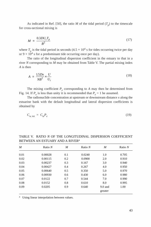
As indicated in Ref. [50], the ratio M of the tidal period (Tp) to the timescalefor cross-sectional mixing is

(17)

where Tp is the tidal period in seconds (4.5 × 104 s for tides occurring twice per dayor 9 × 104 s for a predominant tide occurring once per day).

The ratio of the longitudinal dispersion coefficient in the estuary to that in ariver N corresponding to M may be obtained from Table V. The partial mixing indexA is then

(18)

The mixing coefficient Pe corresponding to A may then be determined fromFig. 14. If Pe is less than unity it is recommended that Pe = 1 be assumed.

The radionuclide concentration at upstream or downstream distance x along theestuarine bank with the default longitudinal and lateral dispersion coefficients isobtained by

Cw, tot = CtePe (19)

ADx

NB

U

Ut= ×15

2

.

MDU T

B

t p=0 3

2

.

43

TABLE V. RATIO N OF THE LONGITUDINAL DISPERSION COEFFICIENTBETWEEN AN ESTUARY AND A RIVERa

0.010.020.030.040.050.060.070.080.09

0.000280.001150.002370.004270.006400.009300.01220.01520.0205

0.10.20.30.40.50.60.70.80.9

0.02400.09000.1670.2670.3500.4300.5440.6100.640

1.02.03.04.05.06.07.08.0

9.0 andgreater

0.7050.9100.9400.9500.9700.9800.9900.9951.00

a Using linear interpolation between values.

M RatioN M RatioN M RatioN

where Cte is obtained from Eq. (16).As for the river,Cte is the completely mixed radionuclide concentration over an

estuarine cross-section. The variable Pe can be regarded as a correction factor forpartial mixing and approaches unity as the downstream distancex increases. (Notethat for x > 0.6B2/D, Pe ª 1 as discussed in Annex VI.)

4.5. COASTAL WATERS

4.5.1. Coastal region modelling approach

The mathematical model selected for coastal waters is based on a steady state,vertically averaged advection–diffusion equation. Further details are provided inAnnex VI. Note that the scale of the mixing length becomes larger as a plume spreadsfurther in the coastal water [51, 52]; the lateral dispersion coefficient in thismethodology changes with downcurrent distance.

44

FIG. 14. Relationship between the estuary partial mixing coefficient and index A.

10 000

1 000

100

10

110–7 10–6 10–5 10–4 10–3 10–2 10–1 1011 10 2

Index A

Est

uary

par

tial m

ixin

g co

rrec

tion

fact

or, P

e

N = 0.0001

0.0003

0.001

0.003

0.010.03

0.1

0.3

1.0

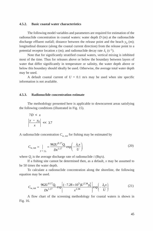
4.5.2. Basic coastal water characteristics

The following model variables and parameters are required for estimation of theradionuclide concentration in coastal waters: water depth D (m) at the radionuclidedischarge effluent outfall; distance between the release point and the beach y0 (m);longitudinal distance (along the coastal current direction) from the release point to apotential receptor location x (m); and radionuclide decay rate li (s–1).

Note that for significantly stratified coastal waters, vertical mixing is inhibitedmost of the time. Thus for releases above or below the boundary between layers ofwater that differ significantly in temperature or salinity, the water depth above orbelow this boundary should ideally be used. Otherwise, the average total water depthmay be used.

A default coastal current of U = 0.1 m/s may be used when site specificinformation is not available.

4.5.3. Radionuclide concentration estimate

The methodology presented here is applicable to downcurrent areas satisfyingthe following conditions (illustrated in Fig. 15).

A radionuclide concentration Cw, tot for fishing may be estimated by

(20)

where Qi is the average discharge rate of radionuclide i (Bq/s).If a fishing site cannot be determined then, as a default,x may be assumed to

be 50 times the water depth.To calculate a radionuclide concentration along the shoreline, the following

equation may be used.

(21)

A flow chart of the screening methodology for coastal waters is shown inFig. 16.

C U Q

Dx

U y

xw tot

i,

.

.

.

.exp

( . )=

− ×

962 7 28 100 17

1 17

5 2 3402

2 34

−

exp

li x

U

C U Q

Dx

x

Uwy y

i i,

.

.exptot = = -Ê

ËÁˆ¯= 0

962 0 17

1 17

l

7

3 70

D x

y y

x

<−

<< .

45

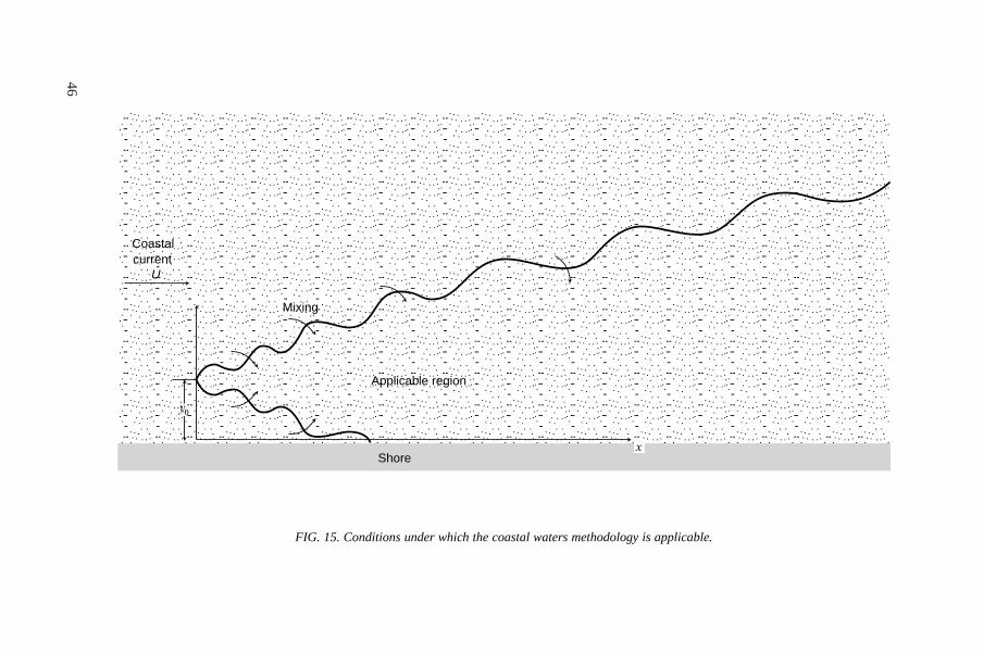
46

FIG. 15. Conditions under which the coastal waters methodology is applicable.

Coastalcurrent

U

y0

Mixing

Applicable region

Shorex

4.6. LAKES AND RESERVOIRS

4.6.1. Classification

For assessment purposes lakes and reservoirs are divided into two types: largeand small. Large lakes are those that have significant wind induced flow and a watersurface area of at least 400 km2. Since a person might be expected to be able to seeacross a distance of around 20 km, as a rough rule a lake can be considered to be largewhen the opposite side of the lake is not visible to a person standing on a 30 m highshore.

4.6.2. Small lakes and reservoirs

For a small lake or reservoir the radionuclide concentration is assumed to beuniform throughout (see Fig. 17).

4.6.2.1. Required parameters

In order to estimate the radionuclide concentration in a small lake or reservoir,the following parameters must be known.

47

FIG. 16. Procedure for calculating radionuclide concentrations in water resulting from dis-charges into coastal waters.

EstimateD, U, y0

Select • For fishing• For shellfish• For shoreline

x

Shoreline:

C = exp exp962U Qi

0.17(–7.28 x 10 U )

5 2.34 2y0 lix

Ux2.34

Dx1.17

Shellfish and fish:

C = expexp962U Qi

0.17lixx

UDx1.17

× × –

–

— The 30 year low annual river flow rate into and out of the lake qr (m3/s) or theriver width (m) under a mean annual river flow rate;

— The lake surface area Al (m2);— The lake volume V (m3) or average lake depth D (m);— The deposition rate from the atmosphere d◊ (Bq◊m–2◊d–1) as described in Section 3;— The expected life of the facility discharging the radionuclide effluent into the

lake,t = T (e.g. 30 years) (s);— The radionuclide decay constant li (s–1).

If the 30 year low annual river flow rate into and out of the lake is not known,it may be estimated as described earlier for rivers and estuaries: the river width, undernormal river flow conditions, is first estimated by direct observation or from a map.The mean annual river flow rate q

–r (m3/s) corresponding to that river width may be

taken from Table III. The 30 year low annual river flow rate qr (m3/s) may beestimated as 1/3 of q

–r (m3/s).

4.6.2.2. Radionuclide concentration estimate

If there is atmospheric deposition of radionuclides on to a small lake and itswatershed, the calculation of radionuclide concentrations in the lake should account

48

FIG. 17. Schematic diagram showing assumed conditions of release into a small lake orreservoir.

River inflow, q r

Concentration = 0

Lake volume V, concentration C

Radionuclidedischarge = F,concentration = C + C 0

Plant intake

River outflow, q r

Concentration = C

Concentration = C

Plant

Radionuclide release rate Qi = FC0

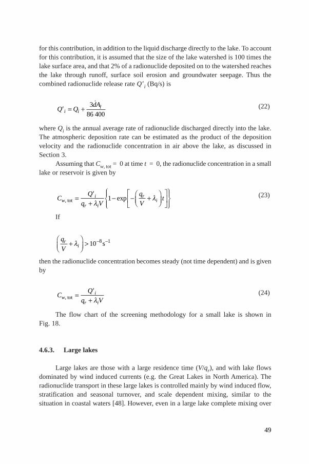
for this contribution, in addition to the liquid discharge directly to the lake. To accountfor this contribution, it is assumed that the size of the lake watershed is 100 times thelake surface area, and that 2% of a radionuclide deposited on to the watershed reachesthe lake through runoff, surface soil erosion and groundwater seepage. Thus thecombined radionuclide release rate Q ′i (Bq/s) is

(22)

where Qi is the annual average rate of radionuclide discharged directly into the lake.The atmospheric deposition rate can be estimated as the product of the depositionvelocity and the radionuclide concentration in air above the lake, as discussed inSection 3.

Assuming that Cw, tot = 0 at time t = 0, the radionuclide concentration in a smalllake or reservoir is given by

(23)

If

then the radionuclide concentration becomes steady (not time dependent) and is givenby

(24)

The flow chart of the screening methodology for a small lake is shown inFig. 18.

4.6.3. Large lakes

Large lakes are those with a large residence time (V/qr), and with lake flowsdominated by wind induced currents (e.g. the Great Lakes in North America). Theradionuclide transport in these large lakes is controlled mainly by wind induced flow,stratification and seasonal turnover, and scale dependent mixing, similar to thesituation in coastal waters [48]. However, even in a large lake complete mixing over

CQ

q Vwi

r i, tot =

+′l

q

Vr

i+ÊËÁ

ˆ¯

> - -l 10 8 1s

CQ

q V

q

Vtw

i

r i

ri, exptot =

+- - +Ê

ËÁˆ¯

È

ÎÍ

˘

˚˙

ÏÌÔ

ÓÔ

¸˝ÔÔ

′l

l1

Q QdA

i il′ = + 3

86 400

49

the entire lake can be achieved in a relatively short period of time (much less than oneyear) owing to a very large dispersion coefficient that changes with distance andseasonal turnover [47]. However, near the release point complete mixing is unlikelyto occur. Thus the long term radionuclide concentration is calculated by using themethodology for partial mixing described in Section 4.4.

50

FIG. 18. Procedure for calculating radionuclide concentrations in water resulting fromdischarge into a small lake or reservoir.

qr

3

= Qi + 3dAl

86 400

Q´

VC =w, tot

C =w, tot

(1– exp [– + li) t]q + Vr il

q + Vr il

qr

V

V

For ( + li) 10 s<–8 –1

For ( + li) > 10 s–8 –1

qr

qr

Estimate • Lake volume V • River inflow q• Lake watershed size A• Atmospheric deposition rat

r

le d

If q is not known r

Use three steps:Estimate B Get q from Table III

q =

•

•

•

r

r

i

Q i

Q i

4.6.3.1. Required parameters

Model parameters required for a large lake include those described inSection 4.4.3.

— The water depthD (m) at the radionuclide discharge effluent outfall,— The distance between the release point in the lake and the beach y0 (m),— The longitudinal distance (along the lake current direction) from the release

point to a potential receptor location x (m),— The radionuclide decay constant li (s–1).

4.6.3.2. Default lake flow velocity

If a site specific lake flow velocity is not available, a default value of U = 0.1 m/smay be used.

4.6.3.3. Radionuclide concentration estimates

The radionuclide concentration is calculated using Eqs (20) and (21) for partialmixing in lake water. The unfiltered radionuclide concentration along theradionuclide plume centreline may be obtained by

A radionuclide concentration along the shoreline is calculated by

As for coastal waters, this methodology is subject to the following conditionsbeing satisfied

A flow chart of the screening methodology for a large lake is shown in Fig. 19.

0

7

–3.7

D x

y y

x

<

<<

0.17 5 2.34 20

, tot 1.17 2.34

962 (–7.28 10 )exp exp –i i

wU Q U y x

CUDx x

lÈ ˘¥ Ê ˆ= Í ˙ Á ˜Ë ¯Í ˙Î ˚

CU Q

Dx

x

Uwi i

,

.

.exptot = -Ê

ËÁˆ¯

962 0 17

1 17

l

51

4.7. SEDIMENT EFFECTS

4.7.1. Sorption and retention

When sediment interacts with radionuclides dissolved in water, theconcentration of the radionuclides in the dissolved phase may be decreased owing toradionuclide adsorption on to sediment particles. Consequently, the concentration ofradionuclides on suspended sediment and the banks and bed of the water body willbe increased owing to adsorption and particle settling. Figure 20 shows the effects ofsediment adsorption and suspended sediment concentration on the radionuclideconcentration.

The distribution coefficient Kd (L/kg) is used to express the exchange ofradionuclides between the dissolved and sediment sorbed phases and is defined for agiven radionuclide as

sediment sorbed radionuclide concentrationper unit weight of sediment (Bq/kg)

Kd = ———————————————————— (24)dissolved radionuclide concentration per unit volume of water (Bq/L)

52

FIG. 19. Procedure for calculating radionuclide concentrations in water resulting fromdischarge into a large lake.

EstimateD, U, y0

Select • For fishing• For shellfish• For shoreline exposure• For drinking water• For irrigation

x

Shoreline and drinking and irrigation water:

C = exp exp962U Qi

0.17(–7.28 x 10 U )

5 2.34 2y0 li x

Ux2.34

Dx1.17

Shellfish and fish:

C = exp962U Qi

0.17li x

UDx1.17

–× ×

×

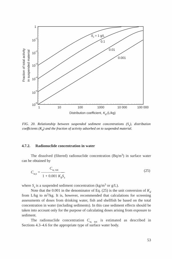
4.7.2. Radionuclide concentration in water

The dissolved (filtered) radionuclide concentration (Bq/m3) in surface watercan be obtained by

Cw, totCw,s = ——————— (25)

1 + 0.001 KdSs

where Ss is a suspended sediment concentration (kg/m3 or g/L).Note that the 0.001 in the denominator of Eq. (25) is the unit conversion of Kd

from L/kg to m3/kg. It is, however, recommended that calculations for screeningassessments of doses from drinking water, fish and shellfish be based on the totalconcentration in water (including sediments). In this case sediment effects should betaken into account only for the purpose of calculating doses arising from exposure tosediment.

The radionuclide concentration Cw, tot is estimated as described inSections 4.3–4.6 for the appropriate type of surface water body.

53

FIG. 20. Relationship between suspended sediment concentrations (Ss), distributioncoefficients (Kd) and the fraction of activity adsorbed on to suspended material.

Frac

tion

of to

tal a

ctiv

ity

in s

uspe

nded

mat

eria

l

Distribution coefficient, K (L/kg)d

102

105

104

103

10–6

101 100 1000 10 000 100 000

S = 1 g/Ls

0.01

0.1

0.001

101

1

–

–

–

–

–

A selection of Kd values associated with suspended sediment in fresh water andsalt water is provided in Table VI [42, 45]. Values of Kd are affected by sediment type,water quality and other conditions [42], and can vary by several orders of magnitudefor each radionuclide. It is therefore important to take care to select a value that isappropriate for the specific site under consideration. If a site specific Kd value is notavailable, default values from Table VI may be used. Usually, the finer the sediment,the higher theKd value for a given radionuclide under the same water qualityconditions [53, 54]. The suspended sediment concentration will vary widelydepending on the characteristics of the water body. Ideally, a site specific value for Ssshould be used, but in the absence of such data the following default values may beused: estuary,Ss = 5 × 10–2 kg/m3; river/lake,Ss = 5 × 10–2 kg/m3; coastal sea,Ss = 1× 10–2 kg/m3.

4.7.3. Radionuclide concentration in suspended sediment

The radionuclide concentration Cs,w (Bq/kg) adsorbed by suspended sedimentcan be obtained by

(26)

When surface water is used for drinking, suspended sediment is removed bywater treatment processes. Thus most of the radionuclide adsorbed on suspendedsediment is removed from drinking water, although the efficiency of removal varieswith radionuclide and with the specific water treatment process used. Theradionuclide concentration in suspended sediment may be important if suspendedsediment is used as a source of surface soil.

4.7.4. Radionuclide concentration in bottom sediment

Bottom sediment can contain radionuclides owing to deposition of suspendedsediment, on which radionuclides are adsorbed, and to direct adsorption on to bottomsediments of dissolved radionuclides from overlying water [45]. Field data [53, 54]suggest much smaller Kd values associated with bottom sediment than withsuspended sediment. This is partly due to the presence of relatively coarser sedimentat the bottom and the greater abundance of bed sediment than of suspended sediment.A notable exception to this is in the null zone of an estuary, where sea water and freshwater merge [57]. The apparent Kd value for bottom sediment is generally assumed tobe one tenth of the Kd value associated with suspended sediment. This assumption isstill likely to overestimate the Kd values of the bottom sediment, with the result that,in the event of this bottom sediment being dredged for use in a landfill, such a Kd

CK C

S KK Cs w

d w

s dd w s,

,,

.

..=

+=

0 001

1 0 0010 001

tot

54

55

TABLE VI. RECOMMENDED SCREENING VALUESFOR Kd (L/kg) FOR ELEMENTS IN NATURALFRESHWATER AND MARINE ENVIRONMENTS,WITH EMPHASIS ON OXIDIZING CONDITIONS

ElementScreening values for Kd (L/kg)

Fresh water a Salt water b

Ac 2 × 106

Ag 1 × 103

Am 5 × 103 2 × 106

AsAtAuBa 5 × 103

BiBrC 5 2 × 103

Cd 2 × 103

Ce 1 × 104 2 × 106

Cm 5 × 103 2 × 106

Co 5 × 103 2 × 105

Cr 1 × 104 c 5 × 104

Cs 1 × 103 3 × 103

CuEu 5 × 102 5 × 105

Fe 5 × 103 5 × 104

GaH 0 c 1Hg 1 × 104

I 10 2 × 101

In 1 × 105

Mn 1 × 103 2 × 105

MoNa 1 Nb 5 × 105

Ni 1 × 105

Np 10 5 × 103

P 50 c 1 × 102 c

Pa 1 × 106

Pb 2 × 105

Pd 5 × 104

Pm 5 × 103 2 × 106

value would lead to a relatively pessimistic dose estimation. Radioactive decay duringaccumulation of the radionuclide on the river bottom is taken into account incalculating the radionuclide concentration in the bottom sediment,Cs,b (Bq/kg), asfollows

(27)

where Te is the effective accumulation time (s).To give a conservative estimate of Cs,b a default value of 3.15 × 107 s (1 year)

is recommended for the effective accumulation periodTe. This value was selected toaccount for the typical situation in which the bottom sediments migrate downstream

CK C

S K

e

TC

e

Ts bd w

s d

T

i es w

T

i e

i e i e

,,

,

( . )( . )

.

–.=

+× = × −− −01 0 001

1 0 001

101

1totλ λ

λ λ

56

TABLE VI. (cont.)

ElementScreening values for Kd (L/kg)

Fresh water a Salt water b

Po 2 × 107

Pu 1 × 105 1 × 105

Ra 500 5 × 103

RbRhRu 500c 3 × 102

S 5 × 10–1

Sb 50c 1 × 103

Se 1 × 103

Sr 1 × 103 1 × 103

Tc 5 1 × 102

Te 1 × 103

Th 1 × 104 2 × 106

Tl 2 × 104

U 50 1 × 103

Y 1 × 107

Zn 500 2 × 104

Zr 1 × 103 1 × 106

a Values for freshwater sediments were taken from Ref. [6],unless otherwise indicated.

b Values for salt water correspond to those for coastalsediment given in Ref. [55], unless otherwise indicated.

c Additional values provided by Y. Onishi [56].

(with the exception of a small lake situation without much river inflow) or are buriedunder more recently deposited layers of sediment. In effect, the sediment layer ofconcern is the most recently deposited material, which has had least opportunity forradioactive decay to occur.

4.7.5. Radionuclide concentration in shore/beach sediment

The surface activity concentration of a radionuclide in shore/beach sediment(Bq/m2), taking account of radioactive decay occurring while the radionuclide isaccumulating in shore or beach sediment, is assumed to be

(28)

where Te is the effective accumulation time (s).The factor of 60 (kg/m2) takes account of the top layer (assumed to be 5 cm)

and bulk density of sediment. A default value ofTe of 3.15 × 107 s (1 year) may beused to provide a conservative estimate ofCs,s.

4.8. UNCERTAINTY

Uncertainty in this methodology arises from possible departures of the realsituation from the assumptions outlined above. Although analytical solution basedmethods such as the current methodology are widely used, rigorous testing toquantify uncertainty under all potential conditions of model application has not beenconducted. The following discussion, nevertheless, gives an indication of theuncertainty to be expected in applying the methodology.

For accurate estimates in partially mixed zones of the water body the surfacegeometry and flow characteristics must be relatively constant. These assumptions areusually satisfied. However, if marked changes in geometry or flow characteristicsoccur between a radionuclide release point and a receptor location, one can performbounding calculations to estimate upper and lower values of radionuclideconcentrations using extreme values for the changing characteristics of flow andgeometry. After complete mixing is achieved, changes in surface geometry and flowcharacteristics are no longer critical.

The sediment adsorption calculation is a potential source of significant error.The ratio of a sediment sorbed radionuclide to a dissolved radionuclide is the productof a distribution coefficient Kd (L/kg) and one 1000th of the suspended sedimentconcentration Ss (kg/m3or g/L). If this product is small, say much less than 1, then theerror in estimating the amount of sediment adsorption is not great. However, if this

CK C

S K TCs s

d w

s d

T

i es

i e

,,( . )( . )

.=

¥ ¥+

¥-

=-0 1 0 001 60

1 0 001

160

tot e l

l ,,b

57

product is much larger than 1, then site specific values of Kd and Ss should beobtained to reduce the potential error in the radionuclide concentration estimate.Figure 20 shows the effects of suspended sediment concentration and the distributioncoefficient on radionuclide concentrations. This figure demonstrates that in mostsurface water cases the potential for the suspended sediment to reduce the dissolvedradionuclide concentration is minor. However, for some radionuclides, such asplutonium and caesium, the sediment effects may be very important [53]. If it isnecessary to evaluate radionuclide distributions with the dynamic effects ofsediment–radionuclide interactions (e.g. radionuclide adsorption/desorption, andtransport, deposition and resuspension of sediment sorbed radionuclides and variableflow conditions), numerical models of these interactions are required [45, 58].

4.9. RADIONUCLIDES DISCHARGED TO SEWERS

In many cases radionuclides are discharged along with other wastes into thesewerage system. In order to estimate the subsequent radiation doses, two extremepossible scenarios may be postulated.

(a) Assume that no radioactive material is retained in the sewage sludge, but that itis all discharged to the water body in liquid form;

(b) Assume that all of the radioactive material discharged is retained in the sewagesludge at the sewage treatment plant.

It is recommended that both situations be considered and the scenario givingthe higher estimated dose be used for screening purposes.

For case (a) the radionuclide concentrations in water and sediment may becalculated as described earlier in this section for discharges into surface water.Subsequent individual radiation doses may be calculated as outlined in Section 6.Case (b) is considered here.

The concentration of a radionuclide in sewage sludge, assuming completetransfer of discharged activity to the sludge, is given by

Csludge = Qsludge/ Ssludge (29)

where

Csludgeis the annual average concentration of the radionuclide in the sludge (Bq/kg),Qsludgeis the annual discharge of the radionuclide (Bq/a),Ssludge is the annual sewage sludge production at the relevant sewage treatment plant

(kg/a).

58

The annual sewage sludge production at the relevant sewage treatment plantwill vary depending on the size of the treatment plant and the size of the populationit serves. In the United Kingdom and Austria a person produces an average of about25–30 kg/a (dry weight) of sewage [59]. This estimate includes both domestic andindustrial sewage (domestic sewage is about 15 kg/a). For screening purposes adefault annual sewage production of 20 kg per person per year (dry weight) isrecommended. A default value for Ssludge(the annual average) can then be obtainedby multiplying this value by the number of people served by the plant. As an example,a typical plant serving 20 000 people would treat about 400 t/a (dry weight). Theexposure pathways arising from sewage sludge are outlined in Section 6 of this SafetyReport. These exposure pathways generally relate to sewage in its wet state. It istherefore necessary to ensure that sludge concentrations relate to wet sludge.Approximately 5% of sewage sludge is comprised of solid material [60], such that thewet weight concentration is 0.05 × concentration (dry weight).

5. TRANSPORT OF RADIONUCLIDES THROUGHTERRESTRIAL AND AQUATIC FOOD CHAINS

Ingestion of radionuclides in foods can be an important contributor to the totaldose received by an individual or population group. An estimate of the radionuclideconcentration is needed to assess such doses. This section describes a genericmethodology to calculate the concentration of radionuclides in human food cropsCv(Bq/kg) and animal produce,Cm (Bq/L) for milk and Cf (Bq/kg) for meat, resultingfrom either an air concentrationCA (Bq/m3) or a ground deposition rate d

·i

(Bq·m–2·d–1) estimated from Section 3, or from a water concentration CW (Bq/m3)estimated from Section 4 (Fig. 2). For the purpose of generic assessments the modelsand default parameters described in this section consider the following processeseither explicitly or implicitly.

(a) Deposition by dry or wet processes;(b) Initial interception and retention by vegetation surfaces;(c) Translocation to the edible tissues of vegetation;(d) Post-deposition retention by vegetation and soil surfaces;(e) Uptake by roots;(f) Adhesion of soil particles on to vegetation surfaces;(g) Direct ingestion of surface soil by humans or grazing animals;(h) Transfer of radionuclides in soil, air, water and vegetation into the milk and

meat of grazing animals;

59

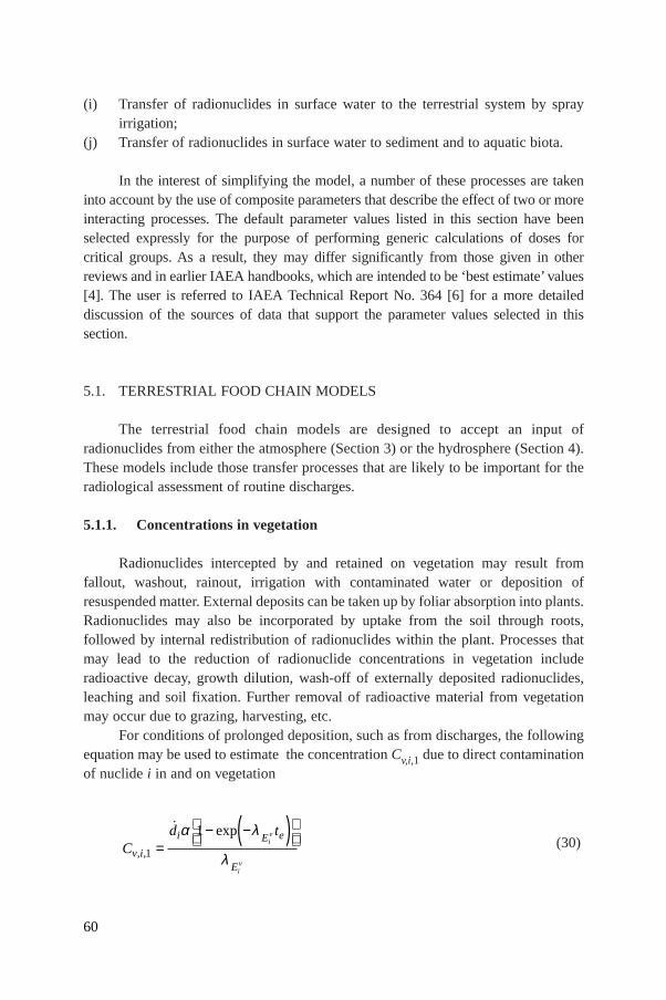
(i) Transfer of radionuclides in surface water to the terrestrial system by sprayirrigation;

(j) Transfer of radionuclides in surface water to sediment and to aquatic biota.

In the interest of simplifying the model, a number of these processes are takeninto account by the use of composite parameters that describe the effect of two or moreinteracting processes. The default parameter values listed in this section have beenselected expressly for the purpose of performing generic calculations of doses forcritical groups. As a result, they may differ significantly from those given in otherreviews and in earlier IAEA handbooks, which are intended to be ‘best estimate’ values[4]. The user is referred to IAEA Technical Report No. 364 [6] for a more detaileddiscussion of the sources of data that support the parameter values selected in thissection.

5.1. TERRESTRIAL FOOD CHAIN MODELS

The terrestrial food chain models are designed to accept an input ofradionuclides from either the atmosphere (Section 3) or the hydrosphere (Section 4).These models include those transfer processes that are likely to be important for theradiological assessment of routine discharges.

5.1.1. Concentrations in vegetation

Radionuclides intercepted by and retained on vegetation may result fromfallout, washout, rainout, irrigation with contaminated water or deposition ofresuspended matter. External deposits can be taken up by foliar absorption into plants.Radionuclides may also be incorporated by uptake from the soil through roots,followed by internal redistribution of radionuclides within the plant. Processes thatmay lead to the reduction of radionuclide concentrations in vegetation includeradioactive decay, growth dilution, wash-off of externally deposited radionuclides,leaching and soil fixation. Further removal of radioactive material from vegetationmay occur due to grazing, harvesting, etc.

For conditions of prolonged deposition, such as from discharges, the followingequation may be used to estimate the concentration Cv,i,1 due to direct contaminationof nuclide i in and on vegetation

(30)Cd t

v i

i E e

E

iv

iv

, ,

˙ exp

1

1=

− −( )

α λ

λ

60

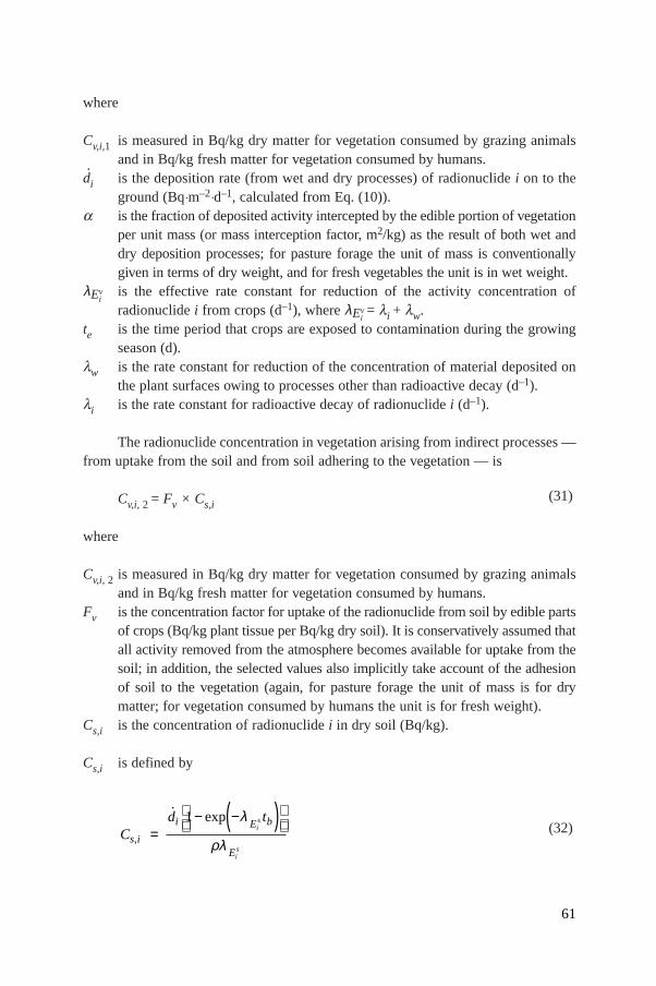
where

Cv,i,1 is measured in Bq/kg dry matter for vegetation consumed by grazing animalsand in Bq/kg fresh matter for vegetation consumed by humans.

d·i is the deposition rate (from wet and dry processes) of radionuclide i on to the

ground (Bq◊m–2◊d–1, calculated from Eq. (10)).a is the fraction of deposited activity intercepted by the edible portion of vegetation

per unit mass (or mass interception factor, m2/kg) as the result of both wet anddry deposition processes; for pasture forage the unit of mass is conventionallygiven in terms of dry weight, and for fresh vegetables the unit is in wet weight.

λEvi

is the effective rate constant for reduction of the activity concentration ofradionuclide i from crops (d–1), where λEv

i= li + lw.

te is the time period that crops are exposed to contamination during the growingseason (d).

lw is the rate constant for reduction of the concentration of material deposited onthe plant surfaces owing to processes other than radioactive decay (d–1).

li is the rate constant for radioactive decay of radionuclidei (d–1).

The radionuclide concentration in vegetation arising from indirect processes —from uptake from the soil and from soil adhering to the vegetation — is

Cv,i, 2 = Fv × Cs,i(31)

where

Cv,i, 2 is measured in Bq/kg dry matter for vegetation consumed by grazing animalsand in Bq/kg fresh matter for vegetation consumed by humans.

Fv is the concentration factor for uptake of the radionuclide from soil by edible partsof crops (Bq/kg plant tissue per Bq/kg dry soil). It is conservatively assumed thatall activity removed from the atmosphere becomes available for uptake from thesoil; in addition, the selected values also implicitly take account of the adhesionof soil to the vegetation (again, for pasture forage the unit of mass is for drymatter; for vegetation consumed by humans the unit is for fresh weight).

Cs,i is the concentration of radionuclidei in dry soil (Bq/kg).

Cs,i is defined by

(32)Cd t

s i

i E b

E

is

is

,

˙ exp=

− −( )

1 λ

ρλ

61

where

λEsi

is the effective rate constant for reduction of the activity concentration in theroot zone of soils (d–1), where λEs

i= li + ls;

ls is the rate constant for reduction of the concentration of material depositedin the root zone of soils owing to processes other than radioactivedecay (d–1);

tb is the duration of the discharge of radioactive material (d);r is a standardized surface density for the effective root zone in soil (kg/m2, dry

soil).

Eq. (32) refers to the total deposit and neglects the amount which is adsorbedto the vegetation. The total concentration of the radionuclide on the vegetation at thetime of consumption is

Cv,i = (Cv,i,1 + Cv,i,2) exp (–lith) (33)

where

Cv,i is measured in Bq/kg dry matter for vegetation consumed by grazing animalsand in Bq/kg fresh matter for vegetation consumed by humans,

li is the rate constant for radioactive decay of radionuclide i (d–1),th is a delay (hold-up) time that represents the time interval between harvest and

consumption of the food (d).

For sprinkler irrigation of cultivated areas Eqs (30) and (32) may be used again.For Eq. (30) the deposition rate is given as

d·i = Cw,i × Iw

(34)

where Cw,i is the concentration of nuclidei in the water (Bq/m3) and Iw is theaverage irrigation rate (m3·m–2·d–1) over the period of irrigation. For Eq. (32) thedeposition rate d

·i from Eq. (34) is multiplied by the fraction of the year over which

the irrigation takes place, in order to provide an annual average irrigation rate.Thus deposition on plant surfaces is calculated with the average irrigation rate overthe irrigation period, while deposition on soil is calculated with the averageirrigation rate over the entire year. The actual rate of irrigation could be muchhigher than an average rate; the use of the appropriate average value will tend tooverestimate the activity accumulated on vegetation or on surface soil, since athigh irrigation rates foliar retention will be decreased and surface runoff increased[6, 61].

62

5.1.1.1. Direct deposition on to plant surfaces

Equation (30) relates to the direct deposition of radionuclides on vegetationfrom the deposition of activity on aerial parts of the plant from either atmospheric orhydrospheric (sprinkler irrigation) sources. The deposition rate from an atmosphericsource may be estimated as described in Section 3.9, while the deposition rate fromirrigation can be derived from the water concentration and irrigation rate, as describedin Section 5.1.1 and Eq. (34). The mass interception factor for forage plants a1 andthe mass interception factor for food crops a2 are specified separately. This isprimarily because vegetation consumed by animals is usually specified on a dryweight basis, while vegetation consumed by humans is most frequently reported asfresh weights; the interception factors reflect this difference. Default values of themass interception fractions a1 and a 2 are listed in Table VII. These values implicitlyinclude the effect of translocation of the radionuclides from foliage to the edibletissues of the vegetation.

5.1.1.2. Reduction of radionuclide concentrations from surfaces of vegetation

The radionuclide concentration in vegetation may be reduced by a variety ofprocesses. These include radioactive decay, wash-off of previously interceptedmaterial by rain or irrigation, surface abrasion and leaf bending from the action of thewind, resuspension, tissue ageing, leaf fall or herbivore grazing, addition of newtissue (growth dilution), volatilization or evaporation [6]. Losses other thanradioactive decay are normally described using an aggregated parameter in the formof a first order rate constant lw. A default value of lw is given in Table VII forestimating the removal of radionuclides from vegetation based on a half-life of14 days. Default values for the crop exposure period (growing season) te , the timeperiod between harvest and consumptionth and the period of soil exposuretb duringthe operating lifetime of a nuclear installation are presented in Table VIII.

5.1.1.3. Deposition on soil

Radionuclides can be deposited on soil either by direct deposition from theatmosphere or from the use of surface water for irrigation. When there is a canopy ofvegetation radionuclides can reach the soil through leaf fall, leaching, wash-off,cuticular sloughing, herbivore excretion and trampling [6]. For the purpose of genericcalculations it is conservatively assumed that the total deposition per unit area reachesthe soil surface, regardless of the extent of canopy cover and subsequent harvestingof vegetation. As indicated earlier, the application of Eq. (32) for irrigation may leadto severe overestimates. This applies particularly for irrigation with water containing

63

anionic radionuclides. Consultation with an expert would be needed for a moreprecise evaluation.

In this generic model discharges and subsequent deposition on the soil areassumed to continue for a periodtb of 30 years. The extent to which this time periodaffects the radionuclide concentration in soil depends on the half-life of theradionuclide and the rate at which the radionuclide becomes unavailable for uptake.The estimated radionuclide concentration in soil is also affected by the assumed depthof soil over which the surface deposition is averaged and by the density of the soil.The density of the soil depends on soil type and extent of soil compaction. For genericcalculations default values of effective surface soil densities r (kg/m2) are given fortwo categories each of depth and soil type in Table IX. Actual values of r may varydepending on the origin, mineral content and classification of the soil [35, 62].However, uncertainties about soil density are relatively small.

64

TABLE VII. CONSERVATIVE VALUES FOR MASS INTERCEPTION ANDENVIRONMENTAL REMOVAL RATES FROM PLANT SURFACES

Parameter Default value

a1 Mass interception factor for forage vegetation (dry weight) 3 m2/kga2 Mass interception factor for food crops (wet weight) 0.3 m2/kglw Environmental removal rate for all plant surfaces 0.05 d–1

TABLE VIII. CONSERVATIVE VALUES FOR CROP AND SOIL EXPOSUREPERIODS AND DELAY TIMES

Parameter te(1) te(2) th(1) th(2) th(3) tb tm tf

Days 30 60 0 90 14 1.1 × 104 1 20

te(1) applies to forage grasses. te(2) applies to food crops.th(1) applies to forage.th(2) applies to stored feed for animals.th(3) applies to food crops.tb refers to a 30 year exposure period (the assumed operating lifetime of a facility).tm is the average time between collection and human consumption of milk.tf is the average time between slaughter and human consumption of meat.

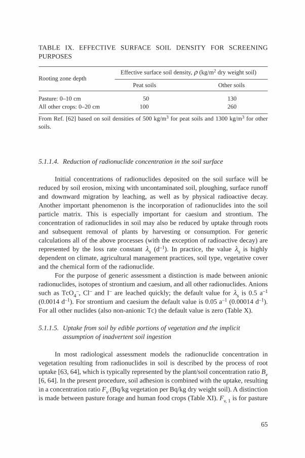
TABLE IX. EFFECTIVE SURFACE SOIL DENSITY FOR SCREENINGPURPOSES

Effective surface soil density,r (kg/m2 dry weight soil)Rooting zone depth

Peat soils Other soils

Pasture: 0–10 cm 50 130All other crops: 0–20 cm 100 260

From Ref. [62] based on soil densities of 500 kg/m3 for peat soils and 1300 kg/m3 for othersoils.

5.1.1.4. Reduction of radionuclide concentration in the soil surface

Initial concentrations of radionuclides deposited on the soil surface will bereduced by soil erosion, mixing with uncontaminated soil, ploughing, surface runoffand downward migration by leaching, as well as by physical radioactive decay.Another important phenomenon is the incorporation of radionuclides into the soilparticle matrix. This is especially important for caesium and strontium. Theconcentration of radionuclides in soil may also be reduced by uptake through rootsand subsequent removal of plants by harvesting or consumption. For genericcalculations all of the above processes (with the exception of radioactive decay) arerepresented by the loss rate constant ls (d–1). In practice, the value ls is highlydependent on climate, agricultural management practices, soil type, vegetative coverand the chemical form of the radionuclide.

For the purpose of generic assessment a distinction is made between anionicradionuclides, isotopes of strontium and caesium, and all other radionuclides. Anionssuch as TcO4

–, Cl– and I– are leached quickly; the default value for ls is 0.5 a–1

(0.0014 d–1). For strontium and caesium the default value is 0.05 a–1 (0.00014 d–1).For all other nuclides (also non-anionic Tc) the default value is zero (Table X).

5.1.1.5. Uptake from soil by edible portions of vegetation and the implicitassumption of inadvertent soil ingestion

In most radiological assessment models the radionuclide concentration invegetation resulting from radionuclides in soil is described by the process of rootuptake [63, 64], which is typically represented by the plant/soil concentration ratioBv[6, 64]. In the present procedure, soil adhesion is combined with the uptake, resultingin a concentration ratioFv (Bq/kg vegetation per Bq/kg dry weight soil). A distinctionis made between pasture forage and human food crops (Table XI).Fv, 1 is for pasture

65

TABLE X. LOSS RATE CONSTANT VALUES FOR SCREENING PURPOSES

Nuclide lS (d–1)

Anions such as TcO4–, Cl– and I– 0.0014a

Sr and Cs 0.00014All other nuclides (including non-anionic forms of Tc and I) 0

a These values apply only if the anions remain in this form. Both TcO4– and I– are easily

reduced in soil. Cl– is never reduced and remains anionic.

vegetation or animal feed (Bq/kg dry weight plant per Bq/kg dry weight soil), whileFv, 2 is for fresh food crops consumed by humans (Bq/kg fresh weight plant per Bq/kgdry weight soil). To account implicitly for soil adhesion, a minimum value of 0.1 isassigned toFv, 1 and 0.001 to Fv, 2. These minimum values are derived as explained inSection 5.1.1.6.

Explicit calculation of soil ingestion by humans and grazing animals willdepend on numerous site specific assumptions that are beyond the scope of a genericassessment. For this, the user is referred to Ref. [6].

5.1.1.6. Derivation of minimum values for Fv, 1 and Fv, 2

Fv, 1 (min) was obtained by assuming (1) that the concentration on the soilsurface of undisturbed pasture is five times higher than the concentration averagedover the 10 cm effective root zone; (2) that 6% of a grazing animal’s diet is composedof surface soil; and (3) that radionuclides ingested with soil are one third as availablefor assimilation in the animal as are radionuclides incorporated into plant tissue[65–67]. Thus

Fv, 1 (min) = 5 × 0.06 × 0.33 ª 0.1

Fv, 2 (min) was obtained by assuming that 0.1% of the human consumption offresh vegetables is composed of soil (2 × 10–4 kg/d dry soil/ 0.2 kg/d = 1 × 10–3). Theradionuclide concentration at the soil surface may be as much as three times higherthan the average calculated for the 20 cm effective root zone for food crops. This highsurface concentration is offset by the assumption that assimilation of radionuclides insoil by humans is one third that for radionuclides in vegetation. Thus

Fv, 2 (min) = (10–3 × 3)/ 3 = 1 × 10–3

66

TABLE XI. ELEMENT SPECIFIC TRANSFER FACTORS FOR TERRESTRIALFOODS FOR SCREENING PURPOSES

Fv, 1 Fv, 2 Fm FfElement forage crops milk meat

(dry weight)a (fresh weight)b (d/L) (d/kg)

Ac 0.1 0.001 2 × 10–6 2 × 10–5

Ag 0.1 0.01 1 × 10–4 0.006Am 0.1 0.002 2 × 10–5 1 × 10–4

Ar 0 0 0 0As 0.2 0.08 1 × 10–4 0.02At 0.9 0.2 0.01 0.01Au 0.4 0.1 1 × 10–5 0.005Ba 0.1 0.05 0.005 0.002Bi 0.5 0.1 0.001 0.002Br 2 0.4 0.02 0.05Cc

Cd 5 0.5 0.02 0.001Ce 0.1 0.05 3 × 10–4 2 × 10–4

Cm 0.1 0.001 2 × 10–6 2 × 10–5

Co 2 0.08 0.01 0.07Cr 0.1 0.001 2 × 10–4 0.09Cs 1d 0.04d 0.01e 0.05e

Cu 2 0.5 0.002 0.01Eu 0.1 0.002 6 × 10–5 0.002Fe 0.1 0.001 3 × 10–4 0.05Ga 0.1 0.003 1 × 10–5 3 × 10–4

Hc

Hg 3 0.3 5 × 10–4 0.01I 0.1 0.02 0.01e 0.05In 0.1 0.003 2 × 10–4 0.004Kr 0 0 0 0Mn 10 0.3 3 × 10–4 7 × 10–4

Mo 1 0.2 0.005 0.01Na 0.6 0.05 0.25 0.8Nb 0.2 0.01 4 × 10–6 3 × 10–6

Ni 1 0.3 0.2 0.05Np 0.5 0.04 5 × 10–5 0.01P 10 1 0.02 0.05Pa 0.1 0.01 5 × 10–6 5 × 10–6

Pb 0.1 0.02 3 × 10–4 7 × 10–4

Pd 0.5 0.1 1 × 10–4 2 × 10–4

Pm 0.1 0.002 6 × 10–5 0.002

67

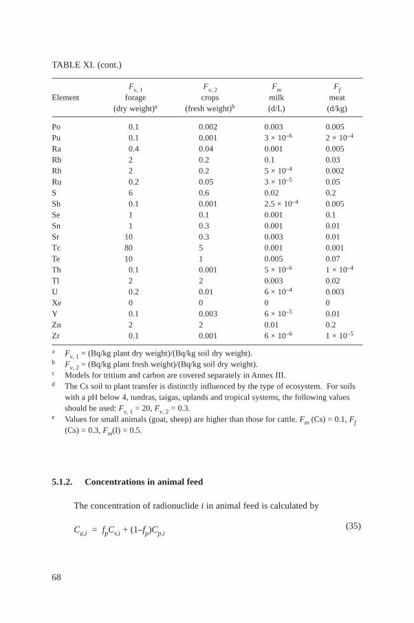
TABLE XI. (cont.)

Fv, 1 Fv, 2 Fm FfElement forage crops milk meat

(dry weight)a (fresh weight)b (d/L) (d/kg)

Po 0.1 0.002 0.003 0.005Pu 0.1 0.001 3 × 10–6 2 × 10–4

Ra 0.4 0.04 0.001 0.005Rb 2 0.2 0.1 0.03Rh 2 0.2 5 × 10–4 0.002Ru 0.2 0.05 3 × 10–5 0.05S 6 0.6 0.02 0.2Sb 0.1 0.001 2.5 × 10–4 0.005Se 1 0.1 0.001 0.1Sn 1 0.3 0.001 0.01Sr 10 0.3 0.003 0.01Tc 80 5 0.001 0.001Te 10 1 0.005 0.07Th 0.1 0.001 5 × 10–6 1 × 10–4

Tl 2 2 0.003 0.02U 0.2 0.01 6 × 10–4 0.003Xe 0 0 0 0Y 0.1 0.003 6 × 10–5 0.01Zn 2 2 0.01 0.2Zr 0.1 0.001 6 × 10–6 1 × 10–5

a Fv, 1 = (Bq/kg plant dry weight)/(Bq/kg soil dry weight).b Fv, 2 = (Bq/kg plant fresh weight)/(Bq/kg soil dry weight).c Models for tritium and carbon are covered separately in Annex III. d The Cs soil to plant transfer is distinctly influenced by the type of ecosystem. For soils

with a pH below 4, tundras, taigas, uplands and tropical systems, the following valuesshould be used:Fv, 1 = 20,Fv, 2 = 0.3.

e Values for small animals (goat, sheep) are higher than those for cattle. Fm (Cs) = 0.1,Ff(Cs) = 0.3,Fm(I) = 0.5.

5.1.2. Concentrations in animal feed

The concentration of radionuclidei in animal feed is calculated by

Ca,i = fpCv,i + (1–fp)Cp,i(35)

68

where

Ca,i is the concentration of radionuclidei in the animal feed (Bq/kg, dry matter);Cv,i is the concentration of radionuclidei for pasture, calculated using Eqs

(30)–(33) withth = 0 (Bq/kg, dry matter);Cp,i is the concentration of radionuclide in stored feeds (Bq/kg, dry weight),

calculated using Eqs (30)–(33), and substitutingCp,i for Cv,i, with th = 90 d;fp is the fraction of the year that animals consume fresh pasture vegetation

(dimensionless).

5.1.3. Intake of radionuclides by animals and transfer to milk and meat

The intake of radionuclides by animals depends on animal species, mass, ageand growth rate of the animal, the digestibility of feed and, in the case of lactatinganimals, the milk yield [6]. For generic calculations grazing animals are assumed tobe cattle which, during the grazing season, are on a diet of fresh pasture only. Thegrazing season depends on latitude, and ranges from a few months to the whole year.

Sources of radionuclides considered for intake by animals are fresh or storedforage and drinking water. The intake of radionuclides with soil has been implicitlyincluded in the soil–plant uptake factorFv. Default values of pasture and waterconsumption for generic milk and meat producing animals are given in Table XII.

The default values for animal intake have been based on values for dairy andbeef cattle. They are conservative, however, and would not be expected substantiallyto underestimate concentrations of radionuclides in milk or meat of other animals.Uptake factors from feed to milk and meat (Fm and Ff, respectively) are provided inTable XI. For caesium and iodine special uptake factors are supplied for smallanimals such as sheep and goats. If the latter factors are used, the food supplyquantities Q (see Table XII) also must be adapted. (Note: it is incorrect to change onlythe food supply quantities Q. Whenever this is done, the values forFm and Ff mustalso be adapted [6].)

5.1.3.1. Concentration in milk

The concentration of a radionuclide in milk depends directly on theradioactivity concentration of the feed consumed by the lactating animal. With thevalue ofCa,i calculated with Eq. (35), and the concentration in drinking waterCw,icalculated in Section 4, the concentration of radionuclidei in milk is estimated as

Cm,i = Fm (Ca,iQm + Cw,iQw) exp (–litm) (36)

69

TABLE XII. ANIMAL INTAKES OF WATER AND DRY MATTER AND THEFRACTION OF THE YEAR THAT ANIMALS CONSUME FRESH PASTURE

Parameter Default value Unit Ref.

Qw (milk, large animal)a 0.06 m3/d [6]Qw (meat, large animal)a 0.04 m3/d [6]Qm (milk, large animal) 16 kg/d (dry weight) [63]Qf (meat, large animal) 12 kg/d (dry weight) [63]fp 0.7 Unitless —

a For small animals such as goats and sheep one tenth of these quantities should be used as adefault.

where

Cm,i is the concentration in milk of radionuclidei (Bq/L),Fm is the fraction of the animal’s daily intake of the radionuclide that appears in

each litre of milk at equilibrium (d/L) (see Table XI),Ca,i is the concentration of radionuclidei in the animal feed (Bq/kg, dry matter),Cw,i is the concentration of radionuclidei in water (Bq/m3),Qm is the amount of feed (in dry matter) consumed by the animal per day (kg/d)

(see Table XII),Qw is the amount of water consumed by the animal per day (m3/d) (see Table XII),li is the rate constant for radioactive decay of radionuclidei (d–1),tm is the average time between collection and human consumption of milk

(assumed to be one day for fresh milk) (see Table VIII).

Default values for Fm are given in Table XI. These values are based on reviewsconsidered in Ref. [6] and values recommended in Ref. [9]. The values in Table XIare specific to dairy cows; however, they are applicable to other lactating animalswithout producing a substantial underestimate of the concentration in the milk ofthese animals. For small animals such as goats and sheep special values are suppliedfor caesium and iodine.

5.1.3.2. Concentration in meat

The radionuclide concentration in meat is calculated in the same way as theconcentration in milk. The same constraints exist.

Cf,i = Fm (Ca,iQf + Cw,iQw) exp (–litf) (37)

where

70

Cf,i is the concentration of radionuclidei in animal flesh (Bq/kg),Ff is the fraction of the animal’s daily intake of a radionuclide that appears in each

kg of flesh at equilibrium or at the time of slaughter (d/kg) (see Table XI),Ca,i is the concentration of radionuclidei in the animal’s feed (Bq/kg, dry matter),Cw,i is the concentration of radionuclide i in water (Bq/m3),Qf is the amount of feed (in dry matter) consumed by the animal per day (kg/d)

(see Table XII),Qw is the amount of water consumed by the animal per day (m3/d) (see Table XII),li is the rate constant for radioactive decay of radionuclide i (d–1),tf is the average time between slaughter and human consumption of meat — a

default value is 20 days (see Table VIII).

The default values for Ff in Table XI are based on data summarized in Ref. [6]and on recommendations in Ref. [9]. Because these values forFm and Ff are intendedfor the purposes of a conservative generic assessment, they may deviate substantiallyfrom the ‘expected’ values published in other reports.

For generic calculations cattle have been selected as the reference herbivore.Although uptake can be expected to vary among species, the values for cattle can beassumed to apply to other meat producing animals. For small animals such as goatsand sheep specific values are supplied for caesium and iodine. Values of Ff , Qf andQw for other animal species are summarized in Ref. [6].

5.1.4. (Semi-)natural terrestrial ecosystems

There is evidence that in some (semi-)natural terrestrial ecosystems thebehaviour of radionuclides may differ from their behaviour in agriculturalecosystems. For example, it appears that caesium remains much more available in(semi-)natural ecosystems at high latitudes. Such caesium may be taken up bymushrooms that are consumed by game. Another example is the accumulation ofcaesium, from atmospheric sources, by lichens that are consumed by reindeer. Forparticular areas higher soil to plant uptake values for caesium are recommended (seeTable XI). These values are sufficiently conservative to account for the increaseduptake in (semi-)natural ecosystems in uplands. A complete treatment of thesephenomena is outside the scope of generic assessment studies; the user is referred toRefs [6, 61].

5.2. AQUATIC FOOD CHAIN TRANSPORT

Radionuclides discharged into the aquatic environment are also assimilated byliving organisms. Some of the assimilated radionuclides are passed along the aquatic

71

food chains and may eventually reach humans. Models are used for dose assessmentsto simulate the transport of radionuclides in aquatic environments.

5.2.1. Basic model

Models that describe the transport of radionuclides from liquid discharges toaquatic foods generally take the form

Caf,i = Cw,iBp/1000 (38)

where

Caf,i is the concentration of radionuclide i in aquatic foodp (Bq/kg);Cw,i is the concentration of dissolved radionuclidei in water (Bq/m3);Bp is the equilibrium ratio of the concentration of radionuclidei in aquatic foodp

to its dissolved concentration in water (Bq·kg–1/Bq·L–1, or L/kg), known as thebioaccumulation factor;

1000 is the conversion factor from m3 to L.

Methods for the generic estimation ofCw,i were considered in Section 4.

5.2.2. Bioaccumulation factor Bp

The transfer of radionuclides from water, through various trophic levels ofaquatic life, to those organisms consumed by humans is condensed into oneparameter — the bioaccumulation factorBp. This parameter is quite variable, withvalues ranging in some cases over several orders of magnitude for a givenradionuclide and organism [6].

The most important factor governing the value of Bp is the trophic level of theorganism. Other factors are

(a) Suspended sediment concentration,(c) Chemical composition of the water body,(d) Chemical state of the released radionuclide,(e) Characteristics specific to the aquatic organism.

For the purpose of these generic calculations default values ofBp (Table XIII)have been selected to ensure that the transfer of dissolved radionuclides from waterto aquatic organisms is conservatively estimated, and to avoid the possibility ofsubstantial underestimation occurring for any specific application. As a result, thevalues given in Table XIII may differ from listings ofBp given in other reports.

72

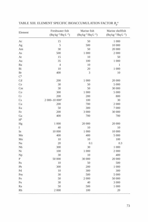
73

TABLE XIII. ELEMENT SPECIFIC BIOACCUMULATION FACTOR Bpa

Element Freshwater fish Marine fish Marine shellfish(Bq·kg–1/Bq·L–1) (Bq·kg–1/Bq·L–1) (Bq·kg–1/Bq·L–1)

Ac 15 50 1 000Ag 5 500 10 000Am 30 50 20 000As 500 1 000 2 000At 15 10 50Au 35 100 1 000Ba 4 10 1Bi 10 20 1 000Br 400 3 10Cb

Cd 200 1 000 20 000Ce 30 50 5 000Cm 30 50 30 000Co 300 1 000 5 000Cr 200 200 800Cs 2 000–10 000c 100 30Cu 200 700 2 000Eu 50 300 7 000Fe 200 3 000 30 000Ga 400 700 700Hb

Hg 1 000 20 000 20 000I 40 10 10In 10 000 1 000 10 000Mn 400 400 5 000Mo 10 10 100Na 20 0.1 0.3Nb 300 30 1 000Ni 100 1 000 2 000Np 30 10 400P 50 000 30 000 20 000Pa 10 50 500Pb 300 200 1 000Pd 10 300 300Pm 30 500 5 000Po 50 2 000 50 000Pu 30 40 3 000Ra 50 500 1 000Rb 2 000 100 20

74

5.2.3. Adjustment of Bp for the effect of suspended sediment

For generic assessment purposes it is often simpler to use the totalconcentrations of radionuclides (Cw, tot) estimated by the equations in Sections 4.3 to4.6 rather than the dissolved radionuclide concentrations estimated in Section 4.7.This introduces conservatism for particle reactive radionuclides because somefraction of these will be adsorbed on to suspended particulate matter and thus will beunavailable for biological uptake. If this pathway is important and better estimates areneeded, then the dissolved concentrations may be estimated (see Section 4.7).

5.2.4. Adjustment of Bp for caesium and strontium in freshwater fish

In Table XIII ranges are given for the values ofBp for strontium and caesium infreshwater fish. For regions with sedimentary bedrock, clay rich soil and hard waterthe lower values should be selected. For regions with igneous bedrock, sandy ororganic soils, and soft water the higher values are appropriate. If dissolved potassiumand suspended sediment concentrations are known, the site specificBp value for

TABLE XIII. (cont.)

Element Freshwater fish Marine fish Marine shellfish(Bq·kg–1/Bq·L–1) (Bq·kg–1/Bq·L–1) (Bq·kg–1/Bq·L–1)

Rh 10 100 1 000Ru 10 2 2 000S 800 2 4Sb 100 400 400Se 200 6 000 6 000Sr 15–75c 2 2Tc 20 30 1 000Te 400 1 000 1 000Th 100 600 1 000Tl 1 000 5 000 5 000U 10 1 30Y 30 20 1 000Zn 1 000 1 000 50 000Zr 300 20 5 000

a Values derived from Refs [6, 55, 68–74].b Models for tritium and carbon are covered separately in Annex III. c See Section 5.2.4 for explanation.

75

caesium can be estimated as described in Ref. [6]. Similarly, if dissolved calciumconcentrations are known, the site specificBp for strontium can be estimated [6, 68].

5.2.5. Biota not included in this Safety Report

Although the categories of aquatic biota presented in Table XIII encompassthose most frequently consumed, it is recognized that in some regions freshwatercrustaceans and marine macroalgae are also consumed.Bp values for freshwatercrustaceans are generally unavailable, but may be assumed to be ten times greaterthan those for freshwater fish, with the exception of caesium, whose Bp value is threetimes lower. For marine macroalgaeBp values are presented in Ref. [55].

5.3. UNCERTAINTY ASSOCIATED WITH THESE PROCEDURES

As discussed earlier, the models and default parameter values presented here areintended for use in calculating doses for screening purposes, such that they are generallylikely to overestimate doses received and are unlikely to underestimate real doses bymore than a factor of ten under any circumstances. They have been based partly onrecommendations for similar models presented elsewhere (see Ref. [9]), where furtherdiscussion on uncertainties is given. Particular points are also made here.

(a) The models for terrestrial food chain transfer are thought to be generallyconservative. In particular, they do not include any allowance for the reductionin radionuclide concentrations owing to food preparation and processing, whichcan be significant.

(b) The models for transfer of radionuclides to milk and meat are based oninformation for cattle. However, it is expected that their use for other animalsshould not lead to substantial underestimation. In particular, the predictedconcentrations in milk should not be more than a factor of three less than theactual concentration, even for milk from other species.

(c) For predicting the transfer of radionuclides to aquatic foods, a simpleconcentration factor approach is adopted through the use of bioaccumulationfactors. These factors have been chosen specifically for screening proceduresand thus are thought to be conservative.

76

6. DOSIMETRIC, HABIT AND OTHER DATA FORDOSE ESTIMATION

The previous sections describe methods for calculating concentrations invarious environmental materials, and other intermediate quantities needed to evaluateradiation doses. In order to complete the dose calculations outlined in Section 2,various dosimetric factors are required. For example, additional data are needed toestimate the annual inhalation dose Einh (Sv/a) and the annual plume immersion doseEimm (Sv/a) from the annual average radionuclide concentration in air CA (Bq/m3),estimated in Section 3, and to estimate the external dose Egr (Sv/a) from radionuclidesdeposited on the ground over a period of 30 years (Fig. 2). Similarly, data are neededto determine doses from the ingestion of food and drinking water, and from externalradiation from radionuclides in aquatic sediments. Dose factors are also needed toestimate doses from sewage sludge from the external pathway and from inhalationof resuspended material from activity on the surface of a sewage sludge containerCsludge (Bq/m2), estimated in Section 4 (Fig. 2). These dosimetric data are discussedin this section, and default values are given for the various cases. In addition, therelevant habit information and other data required to estimate doses are summarized.In each case, data are provided to evaluate the effective dose as defined by the ICRP[2] and the BSS [1]. Information is also provided for calculation of doses to skin andto the lens of the eye.

In some cases, the ingestion or inhalation dose conversion factor associatedwith a particular radionuclide will depend on the chemical or physical form of theradionuclide. For example, the ingestion dose conversion factor for the radionuclide35S depends on whether the material is in the organic or inorganic form. The internaldose conversion factors presented in this section for screening purposes are thehighest reasonable values listed in Ref. [1] for each radionuclide. The dose coefficientvalues given are those recommended in the BSS for all unspecified compounds forthe purpose of calculating doses to workers.

The process involved in calculating doses from atmospheric discharges andfrom discharges to the hydrosphere and to sewerage systems is summarized in Fig 2.

6.1. ESTIMATION OF TOTAL INDIVIDUAL DOSES FROM A SOURCE

The following sections describe how individual doses are calculated for thetransfer of particular radionuclides through particular pathways. For genericassessment purposes the total hypothetical critical group dose due to a particularsource is estimated by summing the doses from all pathways and all radionuclides.Thus the hypothetical critical group is assumed to represent those members of the

public most exposed from the source from all possible pathways. In practice this isunlikely to occur, although it is a reasonable assumption for generic purposes.

As explained earlier, the dose of concern is the maximum dose received duringthe 30th year of discharge. The calculations are based either on the assumption thatequilibrium is reached (e.g. air or water pathways) or on the assumption of acontinuous buildup of long lived radionuclides in the environment (e.g. soil orsediment pathways), as appropriate.

6.2. CALCULATION OF EXTERNAL DOSES FROM AIRBORNERADIONUCLIDES

The annual effective dose from immersion in the atmospheric discharge plumeEim (Sv/a) is given by

Eim = CADFimOf(39)

where

CA is the annual average concentration of nuclide i in air (Bq/m3) calculated inSection 3,

DFim is the effective dose coefficient for immersion (Sv/a per Bq/m),Of is the fraction of the year for which the hypothetical critical group member is

exposed to this particular pathway.

The value of Of will vary depending on the particular circumstances of theexposure. Values of Of applicable for screening purposes are given in Table XIV.

Values of dose coefficients DFim for selected radionuclides, obtained using thesemi-infinite cloud model described below, are given in Table XV. These values arebased on those given in Ref. [75] with additional account of the ingrowth of daughterswith a half-life of less than 30 min. This half-life cut-off was chosen to ensure thatonly those progeny likely to be present relatively close to the site, and therefore toexpose potential critical group members, are taken into account. These values can becombined with the nuclide concentrations in air CA, obtained as described in Section3, to estimate annual hypothetical critical group doses arising from external exposureto the material in the cloud.

The semi-infinite cloud model assumes that radiation from the cloud is inradiative equilibrium, so that the energy absorbed by a given volume element of thecloud is equal to that emitted by the same element. However, near to the ground theradiation source represents only one half of the total solid angle subtended, so that theenergy absorbed in a given volume element is only one half of the energy emitted by

77

78

the same element. This model has been widely used, and several compilations of doseconversion factors relating dose rate with the nuclide concentration in air have beenpublished (see, for example, Refs [76, 77]).

The degree of shielding in a particular building depends on a number of factors,including the structure and the composition of the building materials. Shielding factors

TABLE XIV. DEFAULT VALUES OF HABIT AND OTHER DATA FOREXTERNAL EXPOSURE, INHALATION AND INGESTION DOSE ESTIMATIONFOR A CRITICAL GROUP IN EUROPE

Adult Infant (1 a)

Type of exposure Occupancy Fraction Occupancy Fraction(h/a) Of (h/a) Of

External exposure

Surface contaminated 8760 1 8760 1owing to air deposition

Working/playing over 1600 0.18 1000 0.12contaminated sediments

Submersion in air 8760 1 8760 1

Garden and groundexposure from irrigation 500 0.06 500 0.06

Inhalation

Breathing rate (m3/a) 8400 1400

Ingestion Intake per person

Freshwater fish (kg/a) 30 15

Marine fish (kg/a) 50 25

Marine shellfish (kg/a) 15 0

Water and beverages (m3/a) 0.600 0.260

Fruit, vegetables and 410 150grain, includingpotatoes (kg/a)

Milk (L/a) 250 300

Meat (kg/a) 100 40

79

TABLE XV. EFFECTIVE EXTERNAL DOSE COEFFICIENTS FOR VARIOUSRADIONUCLIDES

Effective dose from Skin dose from Effective dose fromNuclide cloud immersiona cloud immersionb surface depositsc

(Sv/a per Bq/m3) (Sv/a per Bq/m3) (Sv/a per Bq/m2)

Ac-228 1.5 × 10–6 2.5 × 10–6 3.1 × 10–8

Ag-110m 4.3 × 10–6 5.0 × 10–6 8.5 × 10–8

Am-241 2.6 × 10–8 4.0 × 10–8 8.9 × 10–10

As-76 7.0 × 10–7 3.0 × 10–6 1.7 × 10–8

At-211d 5.1 × 10–8 6.2 × 10–8 1.3 × 10–9

Au-198 6.2 × 10–7 1.3 × 10–6 1.3 × 10–8

Bi-206 5.1 × 10–6 6.0 × 10–6 1.0 × 10–7

Bi-210d 8.3 × 10–9 7.3 × 10–7 1.1 × 10–9

Bi-212d 2.3 × 10–6 3.9 × 10–6 4.2 × 10–8

Br-82 4.1 × 10–6 4.9 × 10–6 8.1 × 10–8

Cd-109 9.6 × 10–9 3.1 × 10–8 7.4 × 10–10

Ce-141 1.1 × 10–7 3.2 × 10–7 2.4 × 10–9

Ce-144 1.1 × 10–7 2.7 × 10–6 5.7 × 10–9

Cm-242 1.9 × 10–10 1.4 × 10–9 3.3 × 10–11

Cm-244 1.7 × 10–10 1.2 × 10–9 3.0 × 10–11

Co-58 1.5 × 10–6 1.8 × 10–6 3.0 × 10–8

Co-60 4.0 × 10–6 4.6 × 10–6 7.5 × 10–8

Cr-51 4.8 × 10–8 5.5 × 10–8 9.8 × 10–10

Cs-134 2.4 × 10–6 3.0 × 10–6 4.9 × 10–8

Cs-135 3.0 × 10–10 2.9 × 10–8 1.1 × 10–12

Cs-136 3.4 × 10–6 3.9 × 10–6 6.7 × 10–8

Cs-137d 8.7 × 10–7 1.4 × 10–6 1.8 × 10–8

Cu-64 2.9 × 10–7 5.2 × 10–7 6.0 × 10–9

Eu-154 2.0 × 10–6 2.6 × 10–6 3.8 × 10–8

Eu-155 8.0 × 10–8 1.1 × 10–7 1.9 × 10–9

Fe-55 0 0 0Fe-59 1.9 × 10–6 2.2 × 10–6 3.6 × 10–8

Ga-67 2.3 × 10–7 2.7 × 10–7 4.8 × 10–9

Hg-197 8.5 × 10–8 1.1 × 10–7 2.1 × 10–9

Hg-197m 1.3 × 10–7 3.2 × 10–7 2.8 × 10–9

Hg-203 3.6 × 10–7 4.9 × 10–7 7.4 × 10–9

I-123 2.3 × 10–7 3.0 × 10–7 5.3 × 10–9

I-125 1.7 × 10–8 4.4 × 10–8 1.4 × 10–9

I-129 1.2 × 10–8 3.5 × 10–8 8.3 × 10–10

I-131 5.8 × 10–7 9.4 × 10–7 1.2 × 10–8

I-132 3.6 × 10–6 5.0 × 10–6 7.2 × 10–8

I-133 9.5 × 10–7 1.8 × 10–6 2.0 × 10–8

I-134 4.2 × 10–6 5.9 × 10–6 8.3 × 10–8

80

TABLE XV. (cont.)

Effective dose from Skin dose from Effective dose fromNuclide cloud immersiona cloud immersionb surface depositsc

(Sv/a per Bq/m3) (Sv/a per Bq/m3) (Sv/a per Bq/m2)

I-135 2.6 × 10–6 3.5 × 10–6 4.8 × 10–8

In-111 5.9 × 10–7 7.2 × 10–7 1.2 × 10–8

In-113m 3.9 × 10–7 6.9 × 10–7 8.1 × 10–9

Mn-54 1.3 × 10–6 1.5 × 10–6 2.6 × 10–8

Mo-99d 4.0 × 10–7 1.2 × 10–6 9.2 × 10–9

Na-22 3.4 × 10–6 4.2 × 10–6 6.7 × 10–8

Na-24 7.0 × 10–6 8.7 × 10–6 1.2 × 10–7

Nb-95 1.2 × 10–6 1.4 × 10–6 2.4 × 10–8

Ni-59 0 0 0Ni-63 0 0 0Np-237d 3.3 × 10–8 4.9 × 10–8 7.2 × 10–9

Np-239 2.5 × 10–7 5.0 × 10–7 5.2 × 10–9

P-32 1.7 × 10–8 1.4 × 10–6 2.7 × 10–9

Pa-231 5.5 × 10–8 7.7 × 10–8 1.3 × 10–9

Pa-233 3.0 × 10–7 5.2 × 10–7 6.2 × 10–9

Pb-210d 1.8 × 10–9 4.0 × 10–9 1.2 × 10–9

Pd-103d 2.5 × 10–9 1.2 × 10–8 4.0 × 10–10

Pd-107 0 0 0Pd-109 1.5 × 10–8 6.8 × 10–7 1.3 × 10–9

Pm-147 2.8 × 10–10 2.6 × 10–8 1.1 × 10–12

Po-210 1.3 × 10–11 1.5 × 10–11 2.6 × 10–13

Pu-238 1.7 × 10–10 1.3 × 10–9 2.9 × 10–11

Pu-239 1.4 × 10–10 5.9 × 10–10 1.3 × 10–11

Pu-240 1.6 × 10–10 1.2 × 10–9 2.8 × 10–11

Pu-241d 2.3 × 10–12 3.7 × 10–12 3.0 × 10–11

Pu-242 1.4 × 10–10 1.0 × 10–9 2.3 × 10–11

Ra-224d 1.6 × 10–8 2.1 × 10–8 4.7 × 10–8

Ra-225d 9.7 × 10–9 9.5 × 10–8 8.8 × 10–9

Ra-226d 1.0 × 10–8 1.5 × 10–8 5.7 × 10–8

Rb-86 1.7 × 10–7 1.5 × 10–6 5.4 × 10–9

Rh-105 1.2 × 10–7 3.4 × 10–7 2.5 × 10–9

Rh-107 4.9 × 10–7 1.4 × 10–6 1.1 × 10–8

Ru-103 7.2 × 10–7 8.7 × 10–7 1.5 × 10–8

Ru-106d 3.6 × 10–7 3.4 × 10–6 1.1 × 10–8

S-35 1.0 × 10–10 9.2 × 10–9 5.5 × 10–13

Sb-124 2.9 × 10–6 4.0 × 10–6 5.6 × 10–8

Sb-125d 6.5 × 10–7 8.4 × 10–7 1.4 × 10–8

Se-75 5.9 × 10–7 6.8 × 10–7 1.2 × 10–8

Sn-113d 1.2 × 10–8 2.6 × 10–8 8.8 × 10–9

81

TABLE XV. (cont.)

Effective dose from Skin dose from Effective dose fromNuclide cloud immersiona cloud immersionb surface depositsc

(Sv/a per Bq/m3) (Sv/a per Bq/m3) (Sv/a per Bq/m2)

Sr-85 7.7 × 10–7 8.9 × 10–7 1.6 × 10–8

Sr-87m 4.9 × 10–7 6.8 × 10–7 1.0 × 10–8

Sr-89 1.4 × 10–8 1.2 × 10–6 2.2 × 10–9

Sr-90d 3.1 × 10–9 2.9 × 10–7 3.5 × 10–9

Tc-99 9.2 × 10–10 8.6 × 10–8 2.5 × 10–12

Tc-99m 1.9 × 10–7 2.3 × 10–7 3.9 × 10–9

Te-125m 1.5 × 10–8 6.1 × 10–8 1.2 × 10–9

Te-127m 4.9 × 10–9 2.7 × 10–8 7.0 × 10–10

Te-129m 5.4 × 10–8 4.7 × 10–7 1.9 × 10–9

Te-131md 2.5 × 10–6 3.4 × 10–6 4.9 × 10–8

Te-132d 3.3 × 10–7 4.4 × 10–7 7.9 × 10–8

Th-228d 2.9 × 10–9 4.7 × 10–9 4.7 × 10–8

Th-230d 5.6 × 10–10 1.4 × 10–9 5.7 × 10–8

Th-232d 2.9 × 10–10 1.1 × 10–9 7.8 × 10–8

Tl-201 1.2 × 10–7 1.5 × 10–7 2.8 × 10–9

Tl-202 7.0 × 10–7 8.3 × 10–7 1.5 × 10–8

U-232d 4.7 × 10–10 1.9 × 10–9 4.7 × 10–8

U-234d 2.5 × 10–10 1.3 × 10–9 5.7 × 10–8

U-235d 2.3 × 10–7 2.7 × 10–7 5.3 × 10–9

U-238d 1.2 × 10–10 9.2 × 10–10 6.0 × 10–8

Y-87d 6.9 × 10–7 7.9 × 10–7 2.4 × 10–8

Y-90 2.6 × 10–8 2.0 × 10–6 3.5 × 10–9

Y-91 2.0 × 10–8 1.2 × 10–6 2.4 × 10–9

Zn-65 9.2 × 10–7 1.0 × 10–6 1.8 × 10–8

Zr-95d 1.1 × 10–6 1.4 × 10–6 4.7 × 10–8

a The effective dose values given here have been estimated from the effective dose equivalentvalues for immersion in the cloud, given in Ref. [75], plus the corresponding weighted skindose component, to provide an approximation to effective dose. Additional account of thecontribution from radioactive progeny with half-lives less than 30 min has also been takenwhere appropriate.

b Skin doses from immersion in the cloud are taken from Ref. [75]. Additional account hasbeen taken of radioactive progeny with half-lives less than 30 min, where appropriate. Thesedata are provided to allow comparison with the dose limit for skin. The skin dose componenthas been included in the effective dose coefficients, which are likely to be more useful forother purposes.

c The effective dose values given here have been estimated from the effective dose equivalentvalues for surface deposits, given in Ref. [75], plus the corresponding weighted skin dosecomponent. Additional account has been taken of the contribution from radioactive progenylikely to be important over a period of 30 years (the assumed period of operation anddeposition).

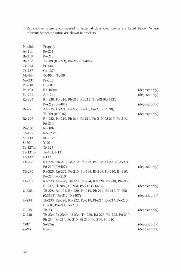
82

d Radioactive progeny considered in external dose coefficients are listed below. Whererelevant, branching ratios are shown in brackets.

Nuclide ProgenyAt-211 Po-211Bi-210 Po-210Bi-212 Tl-208 (0.3593), Po-212 (0.6407)Ce-144 Pr-144Cs-137 Ca-137mMo-99 Tc-99m, Tc-99Np-237 Pa-233Pb-210 Bi-210Pd-103 Rh-103m (deposit only)Pu-241 Am-241 (deposit only)Ra-224 Rn-220, Po-210, Pb-212, Bi-212, Tl-208 (0.3593),

Po-212 (0.6407) (deposit only)Ra-225 Ac-225, Fr-221, At-217, Bi-213, Po-213 (0.978),

Tl-209 (0.0216) (deposit only)Ra-226 Rn-222, Po-210, Pb-214, Bi-214, Po-210, Bi-210, Po-214,

Po-210Ru-106 Rh-106Sb-125 Re-125mSn-113 In-113mSr-90 Y-90Te-127m Te-127Te-131m Te-131, I-131Te-132 I-132Th-228 Ra-224, Rn-220, Po-210, Pb-212, Bi-212, Tl-208 (0.3593),

Po-212 (0.6407) (deposit only)Th-230 Ra-226, Rn-222, Po-210, Pb-214, Bi-214, Po-210, Bi-210,

Po-214, Po-210Th-232 Ra-228, Ac-228, Th-228, Ra-224, Rn-220, Po-210, Pb-212,

Bi-212, Tl-208 (0.3593), Po-212 (0.6407) (deposit only)U-232 Th-228, Ra-224, Rn-220, Po-210, Pb-212, Bi-212, Tl-208

(0.3593), Po-212 (0.6407) (deposit only)U-234 Th-230, Ra-226, Rn-222, Po-210, Pb-214, Bi-214, Po-210,

Bi-210, Po-214, Po-210U-235 Th-231 (deposit only)U-238 Th-234, Pa-234m, U-234, Th-230, Ra-226, Rn-222, Po-210,

Pb-214, Bi-214, Po-210, Bi-210, Po-214, Po-210Y-87 Sr-87m (deposit only)Zr-95 Nb-95 (deposit only)

83

have been found to range from 0.01–0.4 or more [78], with higher values applying towooden houses and lower values applying to multistorey buildings and offices. Thetime an individual will spend indoors depends on a number of factors, such asclimate, occupation and individual habits. On the global scale, the United NationsScientific Committee on the Effects of Atomic Radiation (UNSCEAR) has suggestedthat, on average, 80% of time is spent indoors [78].

For estimation of external exposure the shielding effects of buildings andtime spent indoors could be considered. However, for the purposes of this simplegeneric assessment methodology these considerations do not need to be taken intoaccount.

For evaluation of the effective dose from external exposure, γ radiation fromairborne radionuclides is the main exposure pathway. However, some radionuclidesgive rise to β radiation, which can lead to exposure to the skin. The equivalent doseto skin can be calculated from the annual average concentration of a givenradionuclide in air (see Section 3.2.1) and the dose coefficients for the skin given inTable XV, using Eq. (40)

Eim,s = CADFsOf(40)

where

Eim,s is the annual skin dose from β irradiation (Sv/a),DFs is the skin dose owing to β irradiation per unit air concentration (Sv/a per

Bq/m3).

The coefficients given in Table XV were calculated as described above fromdata in Ref. [75]. The effective dose from skin exposure may be obtained bymultiplying the skin dose by the weighting factor of 0.01 [1, 2].

Some regulatory instruments require the dose to the lens of the eye to becalculated. For purposes of an initial generic assessment the dose to the lens of theeye is assumed to be equal to the dose calculated for the skin.

6.3. CALCULATION OF EXTERNAL DOSES FROM DEPOSITEDACTIVITY

The annual effective dose from ground deposition Egr (Sv/a) is given by

Egr = CgrDFgrOf (41)

where

84

DFgr is the dose coefficient for exposure to ground deposits (Sv/a per Bq/m2),

Cgr is the deposition density of radionuclide i (Bq/m2).

Cgr is obtained from the ground deposition rate d⋅ i calculated in Section 3.9according to the equation

(42)

where

d⋅ i is the total ground deposition rate (Bq⋅m–2⋅d–1) (Section 3.9);λEs

iis the effective rate constant for reduction of the activity in the top 10 to 20 cmof soil (d–1), where λEs

i = λi + λs;

λs is the rate constant for reduction of soil activity owing to processes other thanradioactive decay;

tb is the duration of the discharge of radioactive material (d).

Default values of tb and λs are provided in Section 5 (Tables VIII and X). Valuesfor λi are provided in Annex II.

Table XV gives dose coefficients to estimate the effective dose arising from unitdeposition on the ground for a number of radionuclides. These values have beencalculated on the basis of data given in Ref. [75] for external doses from surfacedeposits. The skin component has been included in the effective dose coefficients, andadditional account has been taken of the ingrowth of progeny likely to make asignificant contribution to external dose over the assumed operational period of 30years. Other compilations of data are also available (e.g. Refs [76, 77]).

For a more realistic estimation of individual doses from this exposure route,particularly for longer lived radionuclides, the effects of migration down the soilcolumn and the shielding effect of overlying layers of soil would need to be taken intoaccount. In addition, shielding afforded by buildings during time spent indoors shouldalso be considered, as discussed in Section 6.2.

6.3.1. Estimating external doses from deposits

The estimation of external dose from material deposited on to the ground is arelatively straightforward procedure, and a number of models exist for this purpose.The simplest way to calculate the dose at a reference height of 1 m above acontaminated surface is to assume that the surface is an infinite plane source on which

Cd ti E b

E

is

is

gr =- -È

Î͢˚

1 exp( )l

l

activity is uniformly distributed. This method is strictly appropriate only forradionuclides with short radioactive half-lives that are deposited on smooth surfaces.For longer lived radionuclides it is necessary to model the migration down throughthe soil column. A number of models have been developed to predict this downwardmovement, but the experimental data to support the models are limited to a fewradionuclides and a few soil types. However, this process may be of considerablesignificance in determining the external exposure over the longer term from thedeposition of long lived, γ emitting radionuclides, and it should be taken into accountfor this purpose. The time variation of the vertical profile of material can then be usedto estimate the exposure above the soil surface, using standard methods [77]. Theshielding provided by overlying layers of soil as a consequence of this downwardmigration of radionuclides through soil is not taken into account in the estimation ofthe dose conversion factors given in Table XV.

6.4. CALCULATION OF EXTERNAL DOSES FROM ACTIVITY INSEDIMENTS

Section 4 describes how to calculate the radionuclide concentrations insediments and water following discharges of radionuclides into rivers, estuaries,coastal waters or lakes, or from deposition from atmospheric discharges on to lakes.That section also gives guidance on the locations for which the concentrations shouldbe calculated, if these are not already known.

External exposure can occur from sediments on tidal flats and along river bankscontaining radionuclides discharged to the water body. Other possible externalexposure pathways may occur, for example as a result of swimming, boating orhandling fishing gear. However, the external dose from time spent on sediment islikely to be much greater than that from the other external aquatic pathways, andtherefore this pathway alone is considered in this simple generic approach.

The annual effective dose due to external exposure Em (Sv/a) from sediment isgiven by

Em = Cs,sDFgrOf(43)

where

Cs,s is the surface activity concentration in shore/beach sediments (Bq/m2) asdescribed in Section 4.7.5,

DFgr is the dose coefficient for exposure to ground deposits (Sv/a per Bq/m2),Of is the fraction of the year for which a hypothetical critical group member is

exposed to this particular pathway.

85

Occupancy times characteristic of the potential critical group members at thesite of interest may be available, but default values representing a hypothetical criticalgroup for use in a generic assessment are given in Table XIV.

6.5. CALCULATION OF INTERNAL DOSES DUE TO INTAKE BYINHALATION AND INGESTION

The internal dose following an intake of radioactive material into the body byinhalation or ingestion is protracted in time after the intake. The effective dosecoefficient from intake will depend on the metabolism, age and life expectancy of theindividual as well as the physicochemical behaviour of the radionuclide concerned.Dose coefficients are usually evaluated using representative ‘reference’ values for thevarious factors, such as those related to metabolism, and are therefore averages eitherfor complete populations or for particular subgroups in a population.

In assessing the exposure of the general public, account has to be taken of theage of the exposed population and of the likely chemical form of radioactive materialin the environment. Partly as a result of the smaller body size of children, dosecoefficients for children are generally greater than those for adults. Although thistends to be counteracted by lower inhalation and ingestion rates, infants and childrenmay receive higher individual doses from a source of exposure than would adults. Inassessing the exposure of hypothetical critical groups, the intakes and effective dosecoefficients appropriate to different ages should ideally be used. Models have beendeveloped to predict the exposure of members of the public of different ages owingto the intake of radionuclides in forms likely to be encountered in the environment(e.g. Ref. [79, 80]). Databases have been compiled of the dose coefficients for intakeby inhalation and ingestion of a large number of radionuclides in a wide range offorms as a function of the age of the individual at the time of intake. The BSS [1]contain a compilation of dose coefficient data for children and adults.

Values of effective dose coefficients for intake by inhalation and ingestion takenfrom Ref. [1] are given in Tables XVI and XVII, respectively. Values are presented forinfants (1–2 years) and adults. A variety of radionuclides are considered and, for each,data are presented for the chemical forms recommended for ‘unspecified compounds’in the BSS (a generally conservative approach). For adults the doses per unit intake areintegrated for 50 years. For infants the doses are integrated to age 70 from the age atintake.

6.5.1. Irradiation from inhaled radionuclides

The annual effective dose from inhalation Einh (Sv/a) is

86

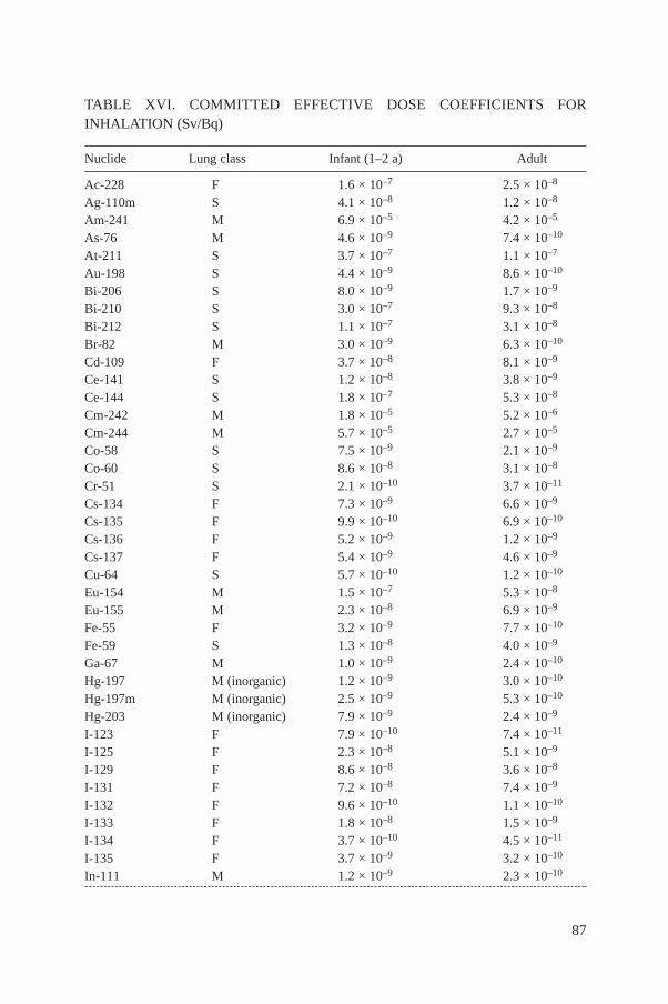
TABLE XVI. COMMITTED EFFECTIVE DOSE COEFFICIENTS FORINHALATION (Sv/Bq)

Nuclide Lung class Infant (1–2 a) Adult

Ac-228 F 1.6 × 10–7 2.5 × 10–8

Ag-110m S 4.1 × 10–8 1.2 × 10–8

Am-241 M 6.9 × 10–5 4.2 × 10–5

As-76 M 4.6 × 10–9 7.4 × 10–10

At-211 S 3.7 × 10–7 1.1 × 10–7

Au-198 S 4.4 × 10–9 8.6 × 10–10

Bi-206 S 8.0 × 10–9 1.7 × 10–9

Bi-210 S 3.0 × 10–7 9.3 × 10–8

Bi-212 S 1.1 × 10–7 3.1 × 10–8

Br-82 M 3.0 × 10–9 6.3 × 10–10

Cd-109 F 3.7 × 10–8 8.1 × 10–9

Ce-141 S 1.2 × 10–8 3.8 × 10–9

Ce-144 S 1.8 × 10–7 5.3 × 10–8

Cm-242 M 1.8 × 10–5 5.2 × 10–6

Cm-244 M 5.7 × 10–5 2.7 × 10–5

Co-58 S 7.5 × 10–9 2.1 × 10–9

Co-60 S 8.6 × 10–8 3.1 × 10–8

Cr-51 S 2.1 × 10–10 3.7 × 10–11

Cs-134 F 7.3 × 10–9 6.6 × 10–9

Cs-135 F 9.9 × 10–10 6.9 × 10–10

Cs-136 F 5.2 × 10–9 1.2 × 10–9

Cs-137 F 5.4 × 10–9 4.6 × 10–9

Cu-64 S 5.7 × 10–10 1.2 × 10–10

Eu-154 M 1.5 × 10–7 5.3 × 10–8

Eu-155 M 2.3 × 10–8 6.9 × 10–9

Fe-55 F 3.2 × 10–9 7.7 × 10–10

Fe-59 S 1.3 × 10–8 4.0 × 10–9

Ga-67 M 1.0 × 10–9 2.4 × 10–10

Hg-197 M (inorganic) 1.2 × 10–9 3.0 × 10–10

Hg-197m M (inorganic) 2.5 × 10–9 5.3 × 10–10

Hg-203 M (inorganic) 7.9 × 10–9 2.4 × 10–9

I-123 F 7.9 × 10–10 7.4 × 10–11

I-125 F 2.3 × 10–8 5.1 × 10–9

I-129 F 8.6 × 10–8 3.6 × 10–8

I-131 F 7.2 × 10–8 7.4 × 10–9

I-132 F 9.6 × 10–10 1.1 × 10–10

I-133 F 1.8 × 10–8 1.5 × 10–9

I-134 F 3.7 × 10–10 4.5 × 10–11

I-135 F 3.7 × 10–9 3.2 × 10–10

In-111 M 1.2 × 10–9 2.3 × 10–10

87

TABLE XVI. (cont.)

Nuclide Lung class Infant (1–2 a) Adult

In-113m M 1.1 × 10–10 2.0 × 10–11

Mn-54 M 6.2 × 10–9 1.5 × 10–9

Mo-99 S 4.8 × 10–9 9.9 × 10–10

Na-22 F 7.3 × 10–9 1.3 × 10–9

Na-24 F 1.8 × 10–9 2.7 × 10–10

Nb-95 S 5.9 × 10–9 1.8 × 10–9

Ni-59 F 8.1 × 10–10 1.8 × 10–10

Ni-63 F 2.0 × 10–9 4.4 × 10–10

Np-237 M 4.0 × 10–5 2.3 × 10–5

Np-239 M 4.2 × 10–9 9.3 × 10–10

P-32 M 1.5 × 10–8 3.4 × 10–9

Pa-231 M 2.3 × 10–4 1.4 × 10–4

Pa-233 S 1.3 × 10–8 3.9 × 10–9

Pb-210 M 3.7 × 10–6 1.1 × 10–6

Pd-103 S 1.8 × 10–9 4.5 × 10–10

Pd-107 S 2.0 × 10–9 5.9 × 10–10

Pd-109 S 1.9 × 10–9 3.7 × 10–10

Pm-147 M 1.8 × 10–8 5.0 × 10–9

Po-210 F 4.8 × 10–6 6.1 × 10–7

Pu-238 M 7.4 × 10–5 4.6 × 10–5

Pu-239 M 7.7 × 10–5 5.0 × 10–5

Pu-240 M 7.7 × 10–5 5.0 × 10–5

Pu-241 M 9.7 × 10–7 9.0 × 10–7

Pu-242 M 7.3 × 10–5 4.8 × 10–5

Ra-224 S 9.2 × 10–6 3.4 × 10–6

Ra-225 S 2.2 × 10–5 7.7 × 10–6

Ra-226 S 2.9 × 10–5 9.5 × 10–6

Rb-86 F 7.7 × 10–9 9.3 × 10–10

Rh-105 S 1.7 × 10–9 3.5 × 10–10

Rh-107 S 9.7 × 10–11 1.7 × 10–11

Ru-103 S 1.0 × 10–8 3.0 × 10–9

Ru-106 S 2.3 × 10–7 6.6 × 10–8

S-35 M 4.5 × 10–9 1.4 × 10–9

Sb-124 M 2.4 × 10–8 6.4 × 10–9

Sb-125 M 1.6 × 10–8 4.8 × 10–9

Se-75 F 6.0 × 10–9 1.3 × 10–9

Sn-113 M 1.0 × 10–8 2.7 × 10–9

Sr-85 S 3.7 × 10–9 8.1 × 10–10

Sr-87m S 1.2 × 10–10 2.1 × 10–11

Sr-89 S 3.0 × 10–8 7.9 × 10–9

Sr-90 S 4.0 × 10–7 1.6 × 10–7

88

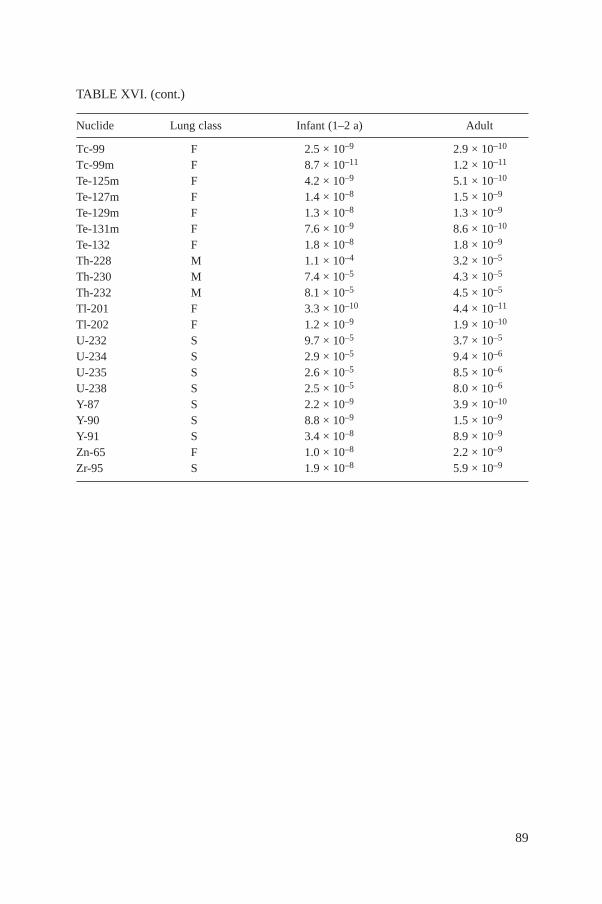
TABLE XVI. (cont.)

Nuclide Lung class Infant (1–2 a) Adult

Tc-99 F 2.5 × 10–9 2.9 × 10–10

Tc-99m F 8.7 × 10–11 1.2 × 10–11

Te-125m F 4.2 × 10–9 5.1 × 10–10

Te-127m F 1.4 × 10–8 1.5 × 10–9

Te-129m F 1.3 × 10–8 1.3 × 10–9

Te-131m F 7.6 × 10–9 8.6 × 10–10

Te-132 F 1.8 × 10–8 1.8 × 10–9

Th-228 M 1.1 × 10–4 3.2 × 10–5

Th-230 M 7.4 × 10–5 4.3 × 10–5

Th-232 M 8.1 × 10–5 4.5 × 10–5

Tl-201 F 3.3 × 10–10 4.4 × 10–11

Tl-202 F 1.2 × 10–9 1.9 × 10–10

U-232 S 9.7 × 10–5 3.7 × 10–5

U-234 S 2.9 × 10–5 9.4 × 10–6

U-235 S 2.6 × 10–5 8.5 × 10–6

U-238 S 2.5 × 10–5 8.0 × 10–6

Y-87 S 2.2 × 10–9 3.9 × 10–10

Y-90 S 8.8 × 10–9 1.5 × 10–9

Y-91 S 3.4 × 10–8 8.9 × 10–9

Zn-65 F 1.0 × 10–8 2.2 × 10–9

Zr-95 S 1.9 × 10–8 5.9 × 10–9

89

TABLE XVII. COMMITTED EFFECTIVE DOSE COEFFICIENTS FORINGESTION (Sv/Bq)

Nuclide Gut transfer factor, f1 Infant (1 a) Adult

Ac-228 5.0 × 10–4 2.8 × 10–9 4.3 × 10–10

Ag-110m 0.050 1.4 × 10–8 2.8 × 10–9

Am-241 5.0 × 10–4 3.7 × 10–7 2.0 × 10–7

As-76 0.500 1.1 × 10–8 1.6 × 10–9

At-211 1.000 7.8 × 10–8 1.1 × 10–8

Au-198 0.100 7.2 × 10–9 1.0 × 10–9

Bi-206 0.050 1.0 × 10–8 1.9 × 10–9

Bi-210 0.050 9.7 × 10–9 1.3 × 10–9

Bi-212 0.050 1.8 × 10–9 2.6 × 10–10

Br-82 1.000 2.6 × 10–9 5.4 × 10–10

Cd-109 0.050 9.5 × 10–9 2.0 × 10–9

Ce-141 5.0 × 10–4 5.1 × 10–9 7.1 × 10–10

Ce-144 5.0 × 10–4 3.9 × 10–8 5.2 × 10–9

Cm-242 5.0 × 10–4 7.6 × 10–8 1.2 × 10–8

Cm-244 5.0 × 10–4 2.9 × 10–7 1.2 × 10–7

Co-58 0.100 4.4 × 10–9 7.4 × 10–10

Co-60 0.100 2.7 × 10–8 3.4 × 10–9

Cr-51 0.100 2.3 × 10–10 3.8 × 10–11

Cs-134 1.000 1.6 × 10–8 1.9 × 10–8

Cs-135 1.000 2.3 × 10–9 2.0 × 10–9

Cs-136 1.000 9.5 × 10–9 3.0 × 10–9

Cs-137 1.000 1.2 × 10–8 1.3 × 10–8

Cu-64 0.500 8.3 × 10–10 1.2 × 10–10

Eu-154 5.0 × 10–4 1.2 × 10–8 2.0 × 10–9

Eu-155 5.0 × 10–4 2.2 × 10–9 3.2 × 10–10

Fe-55 0.100 2.4 × 10–9 3.3 × 10–10

Fe-59 0.100 1.3 × 10–8 1.8 × 10–9

Ga-67 0.001 1.2 × 10–9 1.9 × 10–10

Hg-197 0.020 1.6 × 10–9 2.3 × 10–10

Hg-197m 0.020 3.4 × 10–9 4.7 × 10–10

Hg-203 1.000 1.1 × 10–8 1.9 × 10–9

I-123 1.000 1.9 × 10–9 2.1 × 10–10

I-125 1.000 5.7 × 10–8 1.5 × 10–8

I-129 1.000 2.2 × 10–7 1.1 × 10–7

I-131 1.000 1.8 × 10–7 2.2 × 10–8

I-132 1.000 2.4 × 10–9 2.9 × 10–10

I-133 1.000 4.4 × 10–8 4.3 × 10–9

I-134 1.000 7.5 × 10–10 1.1 × 10–10

I-135 1.000 8.9 × 10–9 9.3 × 10–10

In-111 0.020 1.7 × 10–9 2.9 × 10–10

90

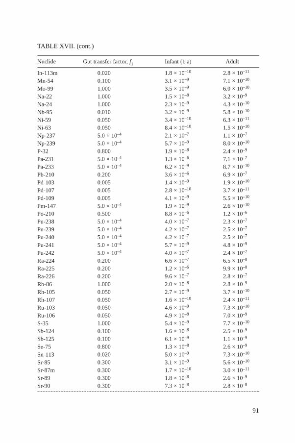
TABLE XVII. (cont.)

Nuclide Gut transfer factor, f1 Infant (1 a) Adult

In-113m 0.020 1.8 × 10–10 2.8 × 10–11

Mn-54 0.100 3.1 × 10–9 7.1 × 10–10

Mo-99 1.000 3.5 × 10–9 6.0 × 10–10

Na-22 1.000 1.5 × 10–8 3.2 × 10–9

Na-24 1.000 2.3 × 10–9 4.3 × 10–10

Nb-95 0.010 3.2 × 10–9 5.8 × 10–10

Ni-59 0.050 3.4 × 10–10 6.3 × 10–11

Ni-63 0.050 8.4 × 10–10 1.5 × 10–10

Np-237 5.0 × 10–4 2.1 × 10–7 1.1 × 10–7

Np-239 5.0 × 10–4 5.7 × 10–9 8.0 × 10–10

P-32 0.800 1.9 × 10–8 2.4 × 10–9

Pa-231 5.0 × 10–4 1.3 × 10–6 7.1 × 10–7

Pa-233 5.0 × 10–4 6.2 × 10–9 8.7 × 10–10

Pb-210 0.200 3.6 × 10–6 6.9 × 10–7

Pd-103 0.005 1.4 × 10–9 1.9 × 10–10

Pd-107 0.005 2.8 × 10–10 3.7 × 10–11

Pd-109 0.005 4.1 × 10–9 5.5 × 10–10

Pm-147 5.0 × 10–4 1.9 × 10–9 2.6 × 10–10

Po-210 0.500 8.8 × 10–6 1.2 × 10–6

Pu-238 5.0 × 10–4 4.0 × 10–7 2.3 × 10–7

Pu-239 5.0 × 10–4 4.2 × 10–7 2.5 × 10–7

Pu-240 5.0 × 10–4 4.2 × 10–7 2.5 × 10–7

Pu-241 5.0 × 10–4 5.7 × 10–9 4.8 × 10–9

Pu-242 5.0 × 10–4 4.0 × 10–7 2.4 × 10–7

Ra-224 0.200 6.6 × 10–7 6.5 × 10–8

Ra-225 0.200 1.2 × 10–6 9.9 × 10–8

Ra-226 0.200 9.6 × 10–7 2.8 × 10–7

Rb-86 1.000 2.0 × 10–8 2.8 × 10–9

Rh-105 0.050 2.7 × 10–9 3.7 × 10–10

Rh-107 0.050 1.6 × 10–10 2.4 × 10–11

Ru-103 0.050 4.6 × 10–9 7.3 × 10–10

Ru-106 0.050 4.9 × 10–8 7.0 × 10–9

S-35 1.000 5.4 × 10–9 7.7 × 10–10

Sb-124 0.100 1.6 × 10–8 2.5 × 10–9

Sb-125 0.100 6.1 × 10–9 1.1 × 10–9

Se-75 0.800 1.3 × 10–8 2.6 × 10–9

Sn-113 0.020 5.0 × 10–9 7.3 × 10–10

Sr-85 0.300 3.1 × 10–9 5.6 × 10–10

Sr-87m 0.300 1.7 × 10–10 3.0 × 10–11

Sr-89 0.300 1.8 × 10–8 2.6 × 10–9

Sr-90 0.300 7.3 × 10–8 2.8 × 10–8

91

TABLE XVII. (cont.)

Nuclide Gut transfer factor, f1 Infant (1 a) Adult

Tc-99 0.500 4.8 × 10–9 6.4 × 10–10

Tc-99m 0.500 1.3 × 10–10 2.2 × 10–11

Te-125m 0.300 6.3 × 10–9 8.7 × 10–10

Te-127m 0.300 1.8 × 10–8 2.3 × 10–9

Te-129m 0.300 2.4 × 10–8 3.0 × 10–9

Te-131m 0.300 1.4 × 10–8 1.9 × 10–9

Te-132 0.300 3.0 × 10–8 3.8 × 10–9

Th-228 5.0 × 10–4 3.7 × 10–7 7.2 × 10–8

Th-230 5.0 × 10–4 4.1 × 10–7 2.1 × 10–7

Th-232 5.0 × 10–4 4.5 × 10–7 2.3 × 10–7

Tl-201 1.000 5.5 × 10–10 9.5 × 10–11

Tl-202 1.000 2.1 × 10–9 4.5 × 10–10

U-232 0.020 8.2 × 10–7 3.3 × 10–7

U-234 0.020 1.3 × 10–7 4.9 × 10–8

U-235 0.020 1.3 × 10–7 4.7 × 10–8

U-238 0.020 1.2 × 10–7 4.5 × 10–8

Y-87 1.0 × 10–4 3.2 × 10–9 5.5 × 10–10

Y-90 1.0 × 10–4 2.0 × 10–8 2.7 × 10–9

Y-91 1.0 × 10–4 1.8 × 10–8 2.4 × 10–9

Zn-65 0.500 1.6 × 10–8 3.9 × 10–9

Zr-95 0.010 5.6 × 10–9 9.5 × 10–10

Einh = CARinhDFinh (44)

where

CA is the radionuclide concentration in air (Bq/m3),Rinh is the inhalation rate (m3/a),DFinh is the inhalation dose coefficient (Sv/Bq) (see Table XVI).

Table XIV gives default inhalation rates for adults and for 1 to 2 year old infants.

6.5.2. Ingestion of radionuclides

Section 5 describes how to calculate the concentration of radionuclides interrestrial and aquatic foodstuffs. The ingestion doses for infants and adults are thencalculated using the following general equation

92

93

Eing, p = Cp,iHpDFing (45)

where

Eing, p is the annual effective dose from consumption of nuclide i in foodstuff p (Sv/a),Cp,i is the concentration of radionuclide i in foodstuff p at the time of consumption

(Bq/kg),Hp is the consumption rate for foodstuff p (kg/a),DFing is the dose coefficient for ingestion of radionuclide i (Sv/Bq).

The default intake rates and dosimetric data are given in Tables XIV, XVII andXVIII.

Equation (45) can also be used to estimate the doses arising from drinkingwater, in which case Hp would be the drinking water intake rate and Cp would be theconcentration of radionuclides in drinking water.

TABLE XVIII. DEFAULT VALUES OF INTAKE PER PERSON FOR VARIOUSCRITICAL GROUPS IN THE WORLD (ADULTS)

Far Near Africa South Central North Europe OceaniaEast East America America America

Water (m3/a) 0.6 0.6 0.6 0.6 0.6 0.6 0.6 0.6

Milk (L/a) 65 140 80 135 155 325 250 410

Meat (kg/a) 40 55 35 90 75 205 100 200

Grain, root 510 600 380 470 445 535 410 500crops,vegetablesand fruits(kg/a)

Freshwater 35 10 15 20 25 25 30 15fish (kg/a)

Marine fish 60 20 30 35 45 40 50 30(kg/a)

Shellfish 20 5 10 10 15 15 15 10(kg/a)

6.6. RADIATION DOSES FROM RADIONUCLIDES IN SEWAGE SLUDGE

Two potential exposure pathways from radionuclides in sewage sludge areconsidered in Fig. 2. These pathways are external irradiation and inhalation ofresuspended material in the sewage plant itself. Other exposure pathways, such asinadvertent ingestion of sludge and those pathways resulting from the disposal of thesludge on to agricultural land, are generally likely to be lower than the predicted dosesto workers in a sewage plant, and thus can be ignored in simple generic dosecalculations. Hypothetical individual doses from each of these pathways arecalculated as follows.

6.6.1. External irradiation exposure

The external irradiation dose from radionuclides in sewage sludge can beestimated in the same way as the dose from material deposited on the ground (Section6.4) and that from activity in sediments (Section 6.5); that is

Es,i = C ′sludgeDFgrOf(46)

where

Es,i is the external radiation dose from sewage sludge for radionuclide i (Sv/a),C ′sludgeis the surface concentration of radionuclide i in sewage sludge (Bq/m2),DFgr is the dose conversion factor for ground contamination (Sv/a per Bq/m2),Of is the fraction of time of exposure per year.

C ′sludge is the surface concentration of the radionuclide per unit area of thesewage sludge. It can be obtained from the calculated concentration of radionuclidesper unit mass of the sludge, calculated as described in Section 4, assuming that thedensity of sewage sludge is 1000 kg/m3 and the depth of the sewage sludge containeris 1 m. Therefore

C ′sludge = Csludge × ρ × depth= Csludge × 1000 (47)

where C sludge is the concentration of radionuclide i in sewage sludge in Bq/kg (wetweight). As explained in Section 4.8, the radionuclide concentration in wet sewagesludge is required. This may be calculated from a dry weight value by multiplying bya conversion factor of 0.05.

Table XV gives values of the ground dose conversion factor for a variety ofradionuclides as discussed in Section 6.3. The fraction of time of exposure per yearcan be taken as 0.228, based on 2000 h/a.

94

6.6.2. Inhalation of resuspended material

Eres = CsludgeRinhDFinhOf DL (48)

where

Eres is the annual dose from inhaling resuspended sewage sludge (Sv/a),Csludge is the concentration of the radionuclide in sewage sludge (Bq/kg wet weight),Rinh is the annual inhalation rate (m3/a),DFinh is the dose coefficient for intake by inhalation (Sv/Bq),Of is the fraction of the year during which exposure occurs,DL is the resuspension factor (kg/m3).

The concentration in sewage sludge is obtained as described in Section 4.However, it should be adjusted to wet weight. The annual inhalation rate is given inTable XIV, and the doses per unit intake by inhalation for various radionuclides aregiven in Table XVI. The default fraction of the year for which workers are exposed is0.228, as above for external exposure to sewage sludge. A default value of 0.1 mg/m3,corresponding to 1 × 10–7 kg/m3, is suggested for the resuspension factor, based onmeasurements made around a sewage plant [81].

7. ESTIMATION OF COLLECTIVE DOSE FORSCREENING PURPOSES

The collective dose may be considered as the product of the number ofindividuals exposed to a source and their average radiation dose. The definition ofcollective dose, together with the aims and methods of assessment, is given in moredetail in Ref. [1]. In this Safety Report the term collective dose is used to refer to thecollective effective dose integrated to infinity, unless otherwise indicated.

Simple collective dose assessments have two main roles in the control ofradioactive discharges to the environment. Firstly, they may form part of thescreening process to demonstrate compliance with a dose limiting criterion. In thiscase an assessment of collective dose is used in conjunction with the assessment ofcritical group doses as discussed in Section 8. Secondly, collective doses may be usedin a simple optimization exercise to compare protection options in a semi-quantitativeway. Modelling procedures for estimating collective doses are similar to those usedto estimate individual doses, except that concentrations of radionuclides inenvironmental compartments extending over large regions, or even globally, are used.

95

In principle, the estimation of collective dose commitments should include allindividual doses, regardless of their magnitude and of when and where they mayoccur. In practice, however, collective doses are calculated for different subgroups ofthe population, and in many cases a distinction is made between local, regional andglobal components. The dispersion of most radionuclides in the environment islimited owing to their short physical half-lives or to removal processes such assedimentation or migration into the deep layers of the soil. Collective doses aretherefore estimated for most radionuclides only in the local and regional zones, whichmay extend from the point of release to distances varying from about 100 km toseveral thousand kilometres. Global assessments are generally performed only forfour radionuclides: 3H, 14C, 85Kr and 129I, which are characterized by relatively longradioactive half-lives and/or a high environmental mobility. Other long livedradionuclides, such as 99Tc or 237Np, may also become globally dispersed followingdischarge. However, they have been little studied and are not considered further here.

To assess the collective dose from an atmospheric discharge, the mainmodelling method involves dividing the region of concern into a number of smallerareas that may be regarded as reasonably homogeneous with respect to population,agricultural practice, etc. The collective dose is then estimated separately for eacharea, and the total is determined by summation. For discharges to the hydrospherecompartment models are generally used to represent dispersion and transfer throughthe environment to humans. The collective doses are then evaluated by summing overpathways and radionuclides. Complex models are available for use in realisticcollective dose estimates or for more detailed assessments such as estimation of thetemporal or geographical distribution of the collective doses [82].

7.1. GENERIC ESTIMATES OF COLLECTIVE DOSE

Models for precise assessments of collective doses are normally relativelycomplex and require the use of computers [82]. UNSCEAR [83] has developedsimple methods for estimating collective doses using generic parameters. Thesemodels must be used with caution and can only provide order of magnitude estimates.

Estimates of collective dose have been made for unit discharges ofradionuclides to the atmosphere and to water bodies. These are intended for screeningor simple generic assessment purposes only. These estimates are based on the resultsof more complex models applied to locations in western Europe [84] and on theresults of simple models based on UNSCEAR methods and using generic, globalparameters. From these results order of magnitude estimates of the collective dose perunit discharge have been obtained, and are given in Table XIX for discharges ofradionuclides to the atmosphere, in Table XX for discharges of radionuclides into

96

marine waters and in Table XXI for discharges of radionuclides into fresh waters.Further information on the origin of these values is given in Annex VII.

It is emphasized that the collective doses given in Tables XIX–XXI are order ofmagnitude estimates only and should be used with caution. They should be used onlyas part of a screening or generic assessment procedure, for example to ensurecompliance with dose limiting criteria or as input to an optimization exercise tocompare options as part of an intuitive, semi-quantitative analysis. They should notbe used for more rigorous optimization analyses, such as cost–benefit analyses, norfor other purposes. The values provided in Tables XIX–XXI are collective dosecommitments, integrated to infinity. For collective doses delivered in the far futurethere exist considerable uncertainties about the sizes, locations and characteristicsof populations. The estimates for long lived radionuclides, particularly for thosethat become globally distributed, should therefore be treated with particularcaution.

8. PROCEDURES TO FOLLOW WHEN ESTIMATED DOSESEXCEED THE SPECIFIED REFERENCE LEVEL

This Safety Report provides an iterative screening approach for assessingcritical group doses resulting from radioactive discharges to the environment. Twotypes of model are provided, the first is a no dilution method that effectively assumesthat members of the public receive exposures at the point of discharge. This approachprovides a quick and easy way to determine whether a further, more refined approachis warranted. Dose calculation factors based on this approach are given in Annex I. Ifthe critical group dose estimated in this way exceeds the relevant dose criterion (e.g.dose constraint), an assessment using a simple generic environmental model thattakes account of dispersion and dilution of discharges in the environment isrecommended. A simple generic environmental model is provided in this reportwhich represents the second stage of the iterative critical group assessment process,illustrated in Fig. 1. This model is described in detail in Sections 3 to 6. Dosecalculation factors based on this model are also presented in Annex I. These factorswere calculated using the data and models presented in this report, together withstandardized assumptions regarding the discharge conditions and the habits andlocation of a hypothetical critical group. The objective of this section is to explain theiterative dose assessment procedure in more detail.

The models presented in this Safety Report represent the first two stages in theiterative assessment approach illustrated in Fig. 21. They are applicable across a widerange of sites and release conditions, and have been designed not to require extensivecollection of site specific data, calculational complexity or expertise in environmental

97

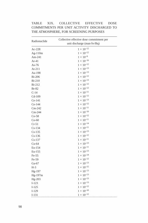
98

TABLE XIX. COLLECTIVE EFFECTIVE DOSECOMMITMENTS PER UNIT ACTIVITY DISCHARGED TOTHE ATMOSPHERE, FOR SCREENING PURPOSES

Radionuclide Collective effective dose commitment perunit discharge (man·Sv/Bq)

Ac-228 1 × 10–12

Ag-110m 1 × 10–12

Am-241 1 × 10–9

Ar-41 1 × 10–16

As-76 1 × 10–12

At-211 1 × 10–13

Au-198 1 × 10–13

Bi-206 1 × 10–12

Bi-210 1 × 10–13

Bi-212 1 × 10–12

Br-82 1 × 10–12

C-14 1 × 10–11

Cd-109 1 × 10–12

Ce-141 1 × 10–13

Ce-144 1 × 10–12

Cm-242 1 × 10–11

Cm-244 1 × 10–10

Co-58 1 × 10–12

Co-60 1 × 10–11

Cr-51 1 × 10–14

Cs-134 1 × 10–11

Cs-135 1 × 10–13

Cs-136 1 × 10–12

Cs-137 1 × 10–11

Cu-64 1 × 10–13

Eu-154 1 × 10–11

Eu-155 1 × 10–13

Fe-55 1 × 10–14

Fe-59 1 × 10–12

Ga-67 1 × 10–13

H-3 1 × 10–15

Hg-197 1 × 10–13

Hg-197m 1 × 10–13

Hg-203 1 × 10–13

I-123 1 × 10–13

I-125 1 × 10–12

I-129 1 × 10–10

I-131 1 × 10–12

99

TABLE XIX. (cont.)

Radionuclide Collective effective dose commitment perunit discharge (man·Sv/Bq)

I-132 1 × 10–12

I-133 1 × 10–12

I-134 1 × 10–12

I-135 1 × 10–12

In-111 1 × 10–13

In-113m 1 × 10–13

Kr-85 1 × 10–17

Kr-89 1 × 10–17

Mn-54 1 × 10–12

Mo-99 1 × 10–13

Na-22 1 × 10–11

Na-24 1 × 10–12

Nb-95 1 × 10–12

Ni-59 1 × 10–13

Ni-63 1 × 10–12

Np-237 1 × 10–10

Np-239 1 × 10–13

P-32 1 × 10–12

Pa-231 1 × 10–10

Pa-233 1 × 10–13

Pb-210 1 × 10–10

Pd-103 1 × 10–14

Pd-107 1 × 10–14

Pd-109 1 × 10–14

Pm-147 1 × 10–14

Po-210 1 × 10–10

Pu-238 1 × 10–9

Pu-239 1 × 10–9

Pu-240 1 × 10–10

Pu-241 1 × 10–11

Pu-242 1 × 10–10

Ra-224 1 × 10–11

Ra-225 1 × 10–11

Ra-226 1 × 10–10

Rb-86 1 × 10–12

Rh-105 1 × 10–13

Rh-107 1 × 10–13

Ru-103 1 × 10–12

Ru-106 1 × 10–12

S-35 1 × 10–12

100

TABLE XIX. (cont.)

Radionuclide Collective effective dose commitment perunit discharge (man·Sv/Bq)

Sb-124 1 × 10–12

Sb-125 1 × 10–12

Se-75 1 × 10–11

Sn-113 1 × 10–13

Sr-85 1 × 10–12

Sr-87m 1 × 10–13

Sr-89 1 × 10–13

Sr-90 1 × 10–11

Tc-99 1 × 10–13

Tc-99m 1 × 10–13

Te-125m 1 × 10–13

Te-127m 1 × 10–13

Te-129m 1 × 10–13

Te-131m 1 × 10–12

Te-132 1 × 10–12

Th-228 1 × 10–10

Th-230 1 × 10–10

Th-232 1 × 10–9

Tl-201 1 × 10–13

Tl-202 1 × 10–12

U-232 1 × 10–10

U-234 1 × 10–9

U-235 1 × 10–10

U-238 1 × 10–10

Xe-133 1 × 10–16

Xe-135 1 × 10–16

Y-87 1 × 10–12

Y-90 1 × 10–13

Y-91 1 × 10–13

Zn-65 1 × 10–11

Zr-95 1 × 10–12

101

TABLE XX. COLLECTIVE EFFECTIVE DOSECOMMITMENTS PER UNIT ACTIVITY DISCHARGEDINTO MARINE WATERS, FOR SCREENING PURPOSES

Radionuclide Collective effective dose commitment perunit discharge (man·Sv/Bq)

Ac-228 1 × 10–18

Ag-110m 1 × 10–13

Am-241 1 × 10–13

As-76 1 × 10–16

At-211 1 × 10–17

Au-198 1 × 10–16

Bi-206 1 × 10–16

Bi-210 1 × 10–16

Bi-212 1 × 10–19

Br-82 1 × 10–19

C-14 1 × 10–11

Cd-109 1 × 10–13

Ce-141 1 × 10–16

Ce-144 1 × 10–14

Cm-242 1 × 10–13

Cm-244 1 × 10–12

Co-58 1 × 10–15

Co-60 1 × 10–13

Cr-51 1 × 10–17

Cs-134 1 × 10–13

Cs-135 1 × 10–14

Cs-136 1 × 10–16

Cs-137 1 × 10–13

Cu-64 1 × 10–17

Eu-154 1 × 10–14

Eu-155 1 × 10–15

Fe-55 1 × 10–13

Fe-59 1 × 10–13

Ga-67 1 × 10–16

H-3 1 × 10–18

Hg-197 1 × 10–15

Hg-197m 1 × 10–15

Hg-203 1 × 10–13

I-123 1 × 10–19

I-125 1 × 10–16

I-129 1 × 10–11

I-131 1 × 10–16

I-132 1 × 10–20

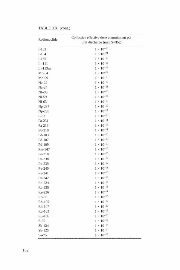
102

TABLE XX. (cont.)

Radionuclide Collective effective dose commitment perunit discharge (man·Sv/Bq)

I-133 1 × 10–18

I-134 1 × 10–21

I-135 1 × 10–19

In-111 1 × 10–16

In-113m 1 × 10–18

Mn-54 1 × 10–14

Mo-99 1 × 10–18

Na-22 1 × 10–17

Na-24 1 × 10–21

Nb-95 1 × 10–16

Ni-59 1 × 10–14

Ni-63 1 × 10–15

Np-237 1 × 10–12

Np-239 1 × 10–17

P-32 1 × 10–13

Pa-231 1 × 10–11

Pa-233 1 × 10–16

Pb-210 1 × 10–11

Pd-103 1 × 10–16

Pd-107 1 × 10–15

Pd-109 1 × 10–17

Pm-147 1 × 10–15

Po-210 1 × 10–10

Pu-238 1 × 10–12

Pu-239 1 × 10–12

Pu-240 1 × 10–11

Pu-241 1 × 10–13

Pu-242 1 × 10–12

Ra-224 1 × 10–14

Ra-225 1 × 10–13

Ra-226 1 × 10–11

Rb-86 1 × 10–15

Rh-105 1 × 10–17

Rh-107 1 × 10–20

Ru-103 1 × 10–15

Ru-106 1 × 10–13

S-35 1 × 10–17

Sb-124 1 × 10–14

Sb-125 1 × 10–14

Se-75 1 × 10–13

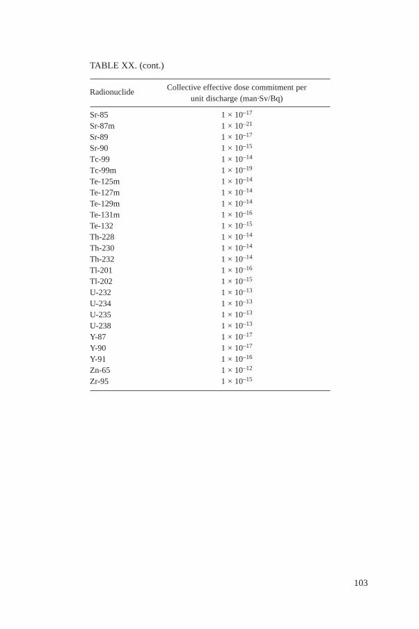
103

TABLE XX. (cont.)

Radionuclide Collective effective dose commitment perunit discharge (man·Sv/Bq)

Sr-85 1 × 10–17

Sr-87m 1 × 10–21

Sr-89 1 × 10–17

Sr-90 1 × 10–15

Tc-99 1 × 10–14

Tc-99m 1 × 10–19

Te-125m 1 × 10–14

Te-127m 1 × 10–14

Te-129m 1 × 10–14

Te-131m 1 × 10–16

Te-132 1 × 10–15

Th-228 1 × 10–14

Th-230 1 × 10–14

Th-232 1 × 10–14

Tl-201 1 × 10–16

Tl-202 1 × 10–15

U-232 1 × 10–13

U-234 1 × 10–13

U-235 1 × 10–13

U-238 1 × 10–13

Y-87 1 × 10–17

Y-90 1 × 10–17

Y-91 1 × 10–16

Zn-65 1 × 10–12

Zr-95 1 × 10–15

104

TABLE XXI. COLLECTIVE EFFECTIVE DOSECOMMITMENTS PER UNIT ACTIVITY DISCHARGED INTOFRESHWATER BODIES, FOR SCREENING PURPOSES

Radionuclide Collective effective dose commitment perunit discharge (man·Sv/Bq)

Ac-228 1 × 10–17

Ag-110m 1 × 10–12

Am-241 1 × 10–11

As-76 1 × 10–16

At-211 1 × 10–16

Au-198 1 × 10–16

Bi-206 1 × 10–15

Bi-210 1 × 10–15

Bi-212 1 × 10–18

Br-82 1 × 10–16

C-14 1 × 10–12

Cd-109 1 × 10–13

Ce-141 1 × 10–15

Ce-144 1 × 10–13

Cm-242 1 × 10–13

Cm-244 1 × 10–11

Co-58 1 × 10–13

Co-60 1 × 10–12

Cr-51 1 × 10–16

Cs-134 1 × 10–11

Cs-135 1 × 10–12

Cs-136 1 × 10–13

Cs-137 1 × 10–11

Cu-64 1 × 10–17

Eu-154 1 × 10–12

Eu-155 1 × 10–13

Fe-55 1 × 10–14

Fe-59 1 × 10–14

Ga-67 1 × 10–16

H-3 1 × 10–14

Hg-197 1 × 10–16

Hg-197m 1 × 10–16

Hg-203 1 × 10–14

I-123 1 × 10–17

I-125 1 × 10–11

I-129 1 × 10–11

I-131 1 × 10–11

I-132 1 × 10–18

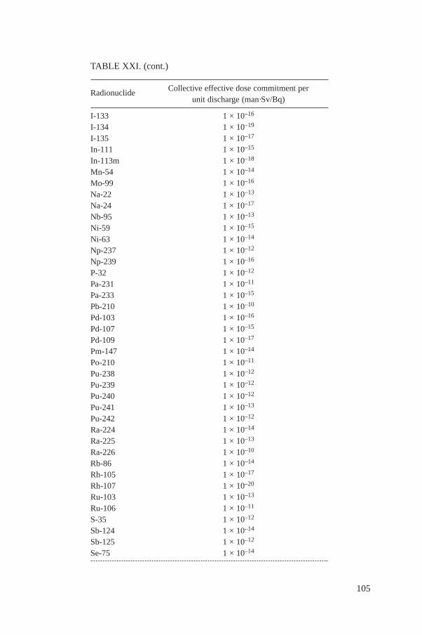
105

TABLE XXI. (cont.)

Radionuclide Collective effective dose commitment perunit discharge (man·Sv/Bq)

I-133 1 × 10–16

I-134 1 × 10–19

I-135 1 × 10–17

In-111 1 × 10–15

In-113m 1 × 10–18

Mn-54 1 × 10–14

Mo-99 1 × 10–16

Na-22 1 × 10–13

Na-24 1 × 10–17

Nb-95 1 × 10–13

Ni-59 1 × 10–15

Ni-63 1 × 10–14

Np-237 1 × 10–12

Np-239 1 × 10–16

P-32 1 × 10–12

Pa-231 1 × 10–11

Pa-233 1 × 10–15

Pb-210 1 × 10–10

Pd-103 1 × 10–16

Pd-107 1 × 10–15

Pd-109 1 × 10–17

Pm-147 1 × 10–14

Po-210 1 × 10–11

Pu-238 1 × 10–12

Pu-239 1 × 10–12

Pu-240 1 × 10–12

Pu-241 1 × 10–13

Pu-242 1 × 10–12

Ra-224 1 × 10–14

Ra-225 1 × 10–13

Ra-226 1 × 10–10

Rb-86 1 × 10–14

Rh-105 1 × 10–17

Rh-107 1 × 10–20

Ru-103 1 × 10–13

Ru-106 1 × 10–11

S-35 1 × 10–12

Sb-124 1 × 10–14

Sb-125 1 × 10–12

Se-75 1 × 10–14

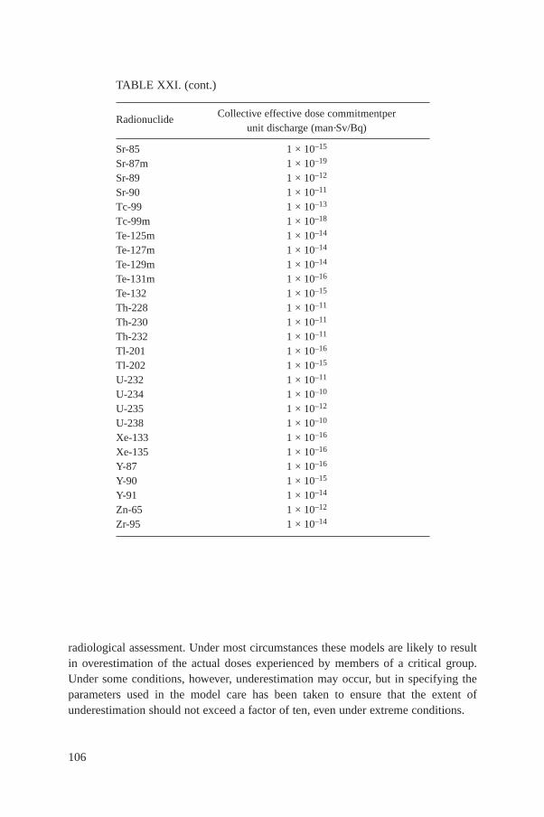
106

radiological assessment. Under most circumstances these models are likely to resultin overestimation of the actual doses experienced by members of a critical group.Under some conditions, however, underestimation may occur, but in specifying theparameters used in the model care has been taken to ensure that the extent ofunderestimation should not exceed a factor of ten, even under extreme conditions.

TABLE XXI. (cont.)

Radionuclide Collective effective dose commitmentperunit discharge (man·Sv/Bq)

Sr-85 1 × 10–15

Sr-87m 1 × 10–19

Sr-89 1 × 10–12

Sr-90 1 × 10–11

Tc-99 1 × 10–13

Tc-99m 1 × 10–18

Te-125m 1 × 10–14

Te-127m 1 × 10–14

Te-129m 1 × 10–14

Te-131m 1 × 10–16

Te-132 1 × 10–15

Th-228 1 × 10–11

Th-230 1 × 10–11

Th-232 1 × 10–11

Tl-201 1 × 10–16

Tl-202 1 × 10–15

U-232 1 × 10–11

U-234 1 × 10–10

U-235 1 × 10–12

U-238 1 × 10–10

Xe-133 1 × 10–16

Xe-135 1 × 10–16

Y-87 1 × 10–16

Y-90 1 × 10–15

Y-91 1 × 10–14

Zn-65 1 × 10–12

Zr-95 1 × 10–14

107

8.1. AN ITERATIVE APPROACH TO EVALUATION

The step-wise iterative procedure recommended in this report to assess criticalgroup doses is illustrated in Fig. 21. This approach has the advantage that it representsan efficient use of assessment resources in that, if applied correctly, it allowsresources to be targeted at those aspects of the assessment that give the highest doses.To apply this method a suitable reference level of dose is needed to indicate when a moreaccurate dose assessment, and the use of a more complex model, is required. It isrecommended that this reference level be set to take account of both the relevant doselimiting criterion and the uncertainty associated with the dose assessment model, asdiscussed in Section 2.1.1.

8.1.1. Initial assessment steps

The first step in this iterative process is to assess doses on the basis of the nodilution model. If doses calculated using this approach are less than the relevant dosecriterion (e.g. dose constraint), no further model complexity is needed, since thisapproach is very conservative and actual doses received would be expected to bemuch lower than those predicted by this method. If doses exceed the dose criterion agreater level of accuracy in the model predictions is warranted and the genericenvironmental model is recommended.

The second step is to apply the generic environmental model. If the criticalgroup doses predicted using this model are less than a reference level (e.g. one tenthof a dose constraint specified by a Regulatory Authority), no further modelcomplexity is needed. However, if doses exceed the reference level a re-evaluation ofthe assumed input data is recommended, as indicated in Fig. 21.

8.1.2. Re-evaluation of input data

The objective of this stage in the process is to review the input data applied inmaking the generic assessment discussed in the previous section, in order todetermine whether they are unduly pessimistic in relation to the conditions at the siteconsidered. Examples of the data that may be considered are discussed below.

8.1.2.1. Estimated discharge rate and conditions

In this process the first step is to re-evaluate the estimated discharge rate andthe conditions of discharge to confirm that they are not overestimates. If the dischargerate has been overestimated the generic dose calculations may be repeated using arevised estimate.

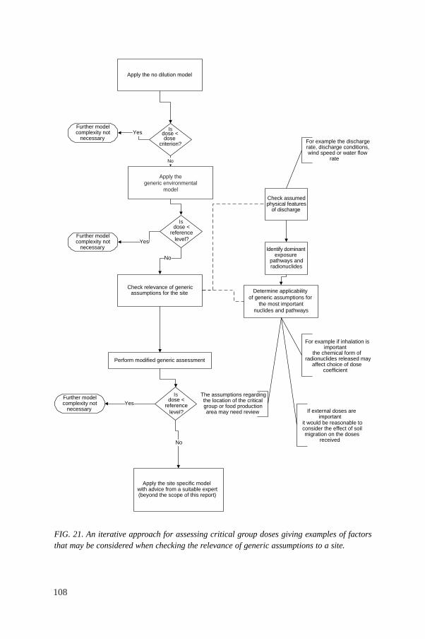
108

FIG. 21. An iterative approach for assessing critical group doses giving examples of factorsthat may be considered when checking the relevance of generic assumptions to a site.

Apply the no dilution model

No

dose <reference level?

YesFurther modelcomplexity not

necessary

No

Check relevance of genericassumptions for the site

Yes

Yes

Apply the site specific modelwith advice from a suitable expert(beyond the scope of this report)

Perform modified generic assessment

Check assumedphysical features

of discharge

Identify dominantexposure

pathways andradionuclides

Determine applicability of generic assumptions for

the most importantnuclides and pathways

For example the dischargerate, discharge conditions,wind speed or water flow

rate

Further modelcomplexity not

necessary

Further modelcomplexity not

necessary

No

For example if inhalation isimportant

the chemical form ofradionuclides released may

affect choice of dosecoefficient

If external doses areimportant

it would be reasonable toconsider the effect of soilmigration on the doses

received

The assumptions regardingthe location of the criticalgroup or food productionarea may need review

Is

dose <reference level?

Is

dose < dose criterion?

Is

Apply thegeneric environmental

model

8.1.2.2. Exposure conditions

If, after review of the discharge rate and discharge conditions, the revisedcalculated doses are still greater than the reference level, it is recommended that theexposure conditions, assumed as part of the generic methodology, should be re-evaluated and revised to reflect more closely the conditions actually prevailing at thesite. This re-evaluation process should begin with those conditions that apply to theradionuclides and exposure pathways that dominate the dose estimate. Any changesin the exposure assumptions that lead to a revised estimate of the hypothetical criticalgroup dose should be accompanied by a detailed justification of these modifications.The variables in the generic methodology that are likely to be most amenable to sitespecific re-evaluation and modification are shown below.

(a) The location of members of the hypothetical critical group and of foodproduction;

(b) Dietary habits and residence times of members of the hypothetical criticalgroup;

(c) Annual average flow rate of a surface water body;(d) Annual average wind speed;(e) Specific exposure pathways;(f) Kd values for the specific site and the specific chemical forms of radionuclides

at the site; (g) If external doses are important, it may be necessary to consider migration of

radionuclides in soil.

After the initial estimates of dose are completed, the dominant radionuclidesand exposure pathways should be identified and evaluated. This evaluation mayreveal that some of the pathways assumed in the generic models are absent at the site.Before these pathways are eliminated from a revised generic calculation, care mustbe taken to account for the presence of other food types not explicitly considered inthe generic methodology. The generic food types included in this methodology areintended to serve as surrogates for any food type that might actually be present. Thusthe generic meat pathway is intended to be sufficiently robust to account for theharvesting of wild game. The generic fish pathway is also intended to account for theconsumption of other aquatic biota that are not specifically identified in the model,including waterfowl. The combined use of the generic pathways of milk, meat andvegetables (including the default values for consumption rates) is intended to accountfor hypothetical critical group consumers of forest mushrooms.

Some of the generic pathways included will, however, always be present at agiven site. For example, if it is possible that people occupy the lands surrounding anatmospheric discharge location, inhalation will always have to be taken into account.

109

Similarly, external exposure to radionuclides deposited on the ground will always haveto be considered if an atmospheric discharge contains γ emitting particulates. Intakesthrough local food products will also be of general relevance, but the distances betweenthe farm or garden where local foods are produced and the discharge location vary.

8.1.3. Final revised generic dose calculations

Once the adjustments for site specific conditions are made, the genericcalculations should be repeated. If the dose estimates still exceed the reference level, itis recommended that the following be considered.

— Reducing the amount discharged,— Modifying the conditions of the discharge,— Consulting professionals in environmental radiological assessments to perform

a detailed site specific assessment.

8.2. REALISTIC DOSE ASSESSMENTS IN CONSULTATION WITHQUALIFIED PROFESSIONALS USING MORE ACCURATE MODELS

If the revised calculations remain above the reference level, and it is notreasonable either to reduce the amount discharged or modify the conditions of thedischarge, a more detailed site specific assessment of the dose to members of thecritical group should be considered. Such an assessment should be performed byqualified professionals who are able to calculate hypothetical doses using both moreaccurate models and more realistic estimates of parameter values. The models,assumptions and parameter values used in the assessment should be documented andmade available for review by competent authorities. Recommendations for qualifiedprofessionals and for more accurate models can be obtained by contacting the IAEA.

When realistic dose estimates are made it is advisable to quantify sources ofuncertainty and to propagate these through the calculations to produce a statement ofconfidence (e.g. a 95% subjective confidence interval) about the dose estimate [5].The dose estimate and its confidence bounds can then be compared with the relevantdose limiting criterion. If the upper confidence bound of the dose estimate is abovethis criterion, efforts should be made either to reduce the uncertainty in the sitespecific dose estimate or to reduce the amount discharged.

Uncertainty is most effectively reduced by collecting additional data on thosecomponents of the model that dominate the uncertainty in the dose estimate. Thedominant components can be identified through a quantitative uncertainty analysisperformed in conjunction with a sensitivity analysis. The procedures of quantitativeuncertainty and sensitivity analysis are described in detail in Ref. [5].

110

If the lower confidence bound of the dose estimated using the more accuratemethods exceeds the relevant dose limiting criterion, and if this effect is confirmedthrough external review by qualified individuals, then there should be a high degreeof confidence that actual doses will exceed the criterion. Further investigation is notlikely to be justified. Although additional studies should lead to improved confidencein the dose estimate, the fact that the dose limiting criteria are violated will merely beconfirmed. Under these circumstances, the only remaining options are to

— Reduce the amount discharged and repeat the assessment,— Modify the conditions under which the discharge occurs and repeat the

assessment,— Abandon the practice or operation,— Apply for a special case variance from the relevant dose limiting criterion.

These issues are discussed in more detail in Ref. [3].

REFERENCES

[1] FOOD AND AGRICULTURE ORGANIZATION OF THE UNITED NATIONS,INTERNATIONAL ATOMIC ENERGY AGENCY, INTERNATIONAL LABOURORGANISATION, OECD NUCLEAR ENERGY AGENCY, PAN AMERICANHEALTH ORGANIZATION, WORLD HEALTH ORGANIZATION, InternationalBasic Safety Standards for Protection against Ionizing Radiation and for the Safety ofRadiation Sources, Safety Series No. 115, IAEA, Vienna (1996).

[2] INTERNATIONAL COMMISSION ON RADIOLOGICAL PROTECTION, 1990Recommendations of the International Commission on Radiological Protection,Publication 60, Pergamon Press, Oxford and New York (1991).

[3] INTERNATIONAL ATOMIC ENERGY AGENCY, Regulatory Control of RadioactiveDischarges to the Environment, Safety Standards No. WS-G-2.3, IAEA, Vienna (2000).

[4] INTERNATIONAL ATOMIC ENERGY AGENCY, Generic Models and Parameters forAssessing the Environmental Transfer of Radionuclides from Routine Releases:Exposures of Critical Groups, Safety Series No. 57, IAEA, Vienna (1982).

[5] INTERNATIONAL ATOMIC ENERGY AGENCY, Evaluating the Reliability ofPredictions Made Using Environmental Transfer Models, Safety Series No. 100, IAEA,Vienna (1989).

[6] INTERNATIONAL ATOMIC ENERGY AGENCY, Handbook of Parameter Values forthe Prediction of Radionuclide Transfer in Temperate Environments, Technical ReportsSeries No. 364, IAEA, Vienna (1994).

111

112

[7] TILL, J.E., MEYER, H.R. (Eds), Radiological Assessment. A Textbook onEnvironmental Dose Analysis, Rep. NUREG/CR-3332, ORNL-5968, United StatesNuclear Regulatory Commission, Washington, DC (1983).

[8] NATIONAL COUNCIL ON RADIATION PROTECTION AND MEASUREMENTS,Screening Techniques for Determining Compliance with Environmental Standards.Releases of Radionuclides to the Atmosphere, NCRP Commentary No. 3, Revision plusAddendum, NCRP, Bethesda, MD (1989).

[9] NATIONAL COUNCIL ON RADIATION PROTECTION AND MEASUREMENTS,Screening Models for Releases of Radionuclides to Atmosphere, Surface Water, andGround, Rep. 123 I, NCRP, Bethesda, MD (1996).

[10] NATIONAL COUNCIL ON RADIATION PROTECTION AND MEASUREMENTS,Screening Models for Releases of Radionuclides to Atmosphere, Surface Water, andGround — Work Sheets, Rep. 123 II, NCRP, Bethesda, MD (1996).

[11] INTERNATIONAL ATOMIC ENERGY AGENCY, Atmospheric Dispersion in NuclearPower Plant Siting: A Safety Guide, Safety Series No. 50-SG-S3, IAEA, Vienna (1980).

[12] HEINEMANN, K., VOGT, K.J., “Statistical studies on the limitation of short-timereleases from nuclear facilities”, Congress of the International Radiation ProtectionAssociation (Proc. 5th Congr. Jerusalem, 1980), Vol. 2, IRPA, Washington, DC (1980)67–70.

[13] GIFFORD, F.A., “Diffusion in the lower layers of the atmosphere”, Meteorology andAtomic Energy (SLADE, D.H., Ed.), Rep. TID-24 190, United States Atomic EnergyCommission, Washington, DC (1968) 65.

[14] NATIONAL COUNCIL ON RADIATION PROTECTION AND MEASUREMENTS,Radiological Assessment: Predicting the Transport, Bioaccumulation, and Uptake byMan of Radionuclides Released to the Environment, Rep. 76, NCRP, Bethesda, MD(1984).

[15] PASQUILL, F., SMITH, F.B., Atmospheric Diffusion, 3rd edn, Ellis Horwood,Chichester (1983).

[16] VOGT, K.J., “Atmosphärische Ausbreitungen und Ablagerungen radioaktiver Stoffe”,Radioökologie, Berichtsband der Fachtagung Radioökologie des DeutschenAtomforums e.V., Bonn, 1979, Vulkan-Verlag, Essen (1979).

[17] CLARKE, R.H., A Model for Short and Medium Range Dispersion of RadionuclidesReleased to the Atmosphere. The First Report of a Working Group on AtmosphericDispersion, Rep. NRPB-R91, National Radiological Protection Board, Chilton (1979).

[18] BRENK, H.D., VOGT, V.J., The calculation of wet deposition from radioactive plumes,Nucl. Safety 22 (1981) 362–371.

[19] HEINEMANN, K., VOGT, K.J., Measurements of the deposition of iodine ontovegetation and of the biological halflife of iodine on vegetation, Health Phys. 39 (1980)463–474.

[20] HORBERT, M., VOGT, K.J., ANGELETTI, L., Untersuchungen zur Ablagerung vonAerosolen auf Vegetation und anderen Grenzflächen, Rep. Jül-1288,Kernforschungsanlage, Jülich (1976).

113

[21] JONES, J.A., The Estimation of Long Range Dispersion and Deposition of ContinuousReleases of Radionuclides to the Atmosphere, Rep. NRPB-R123, National RadiologicalProtection Board, Chilton (1981).

[22] BAYER, A., Die Radiologische Belastung der Bevölkerung der Rhein-Maas-Region,Rep. V/1647/77D, Commission of the European Communities, Luxembourg (1978).

[23] THUILLIERE, R.H., MANCUSO, R.L., Building Effects on Effluent Dispersion fromRoof Vents at Nuclear Power Plants, Rep. EPRI NP-1380, Electric Power ResearchInstitute, Palo Alto, CA (1980).

[24] HOSKER, R.P., “Flow and diffusion near obstacles”, Atmospheric Sciences and PowerProduction (RANDERSON, D., Ed.), Rep. DOE/TIC-27601, Department of Energy,Washington, DC (1984).

[25] NATIONAL COUNCIL ON RADIATION PROTECTION AND MEASUREMENTS,Uncertainty in NCRP Screening Models Relating to Atmospheric Transport, Depositionand Uptake by Humans, NCRP Commentary No. 8, NCRP, Bethesda, MD (1993).

[26] GIFFORD, F.A., Jr., HANNA, S.R., “Dispersion of sulfur dioxide emission from areasources”, Power Generation: Air Pollution Monitoring and Control (NOLL, K.E.,DAVIS, W.T., Eds), Ann Arbor Science Publishers, Inc., Ann Arbor, MI (1975).

[27] WILSON, D.J., BRITTER, R.E., Estimates of building surface concentrations fromnearby point sources, Atmos. Environ. 16 (1982) 2631–2646.

[28] BRIGGS, G.A., Diffusion Estimation for Small Emissions, 1973 Ann. Rep.,Environmental Research Laboratories, Oak Ridge, TN (1974).

[29] GEISS, H., NESTER, K., THOMAS, P., VOGT, K.J., in der Bundesrepublik Deutschlandexperimentell ermittelte Ausbreitungsparameter für 100 m Emissionshöhe, Reps Jül-1707,KfK-3095, Kernforschungsanlage Jülich/Kernforschungszentrum, Karlsruhe (1981).

[30] VOGT, K.J., GEISS, H., Neue Ausbreitungskoeffizienten für 50 und 100 mEmissionshöhe, Internal Rep., Kernforschungsanlage, Jülich (1980).

[31] HÜBSCHMANN, W., NESTER, K., THOMAS, P., Ausbreitungsparameter fürEmissionshöhen von 160 m und 195 m, Rep. KfK-2939, Kernforschungszentrum,Karlsruhe (1980) 182.

[32] MILLER, C.W., YILDIRAN, M., Estimating radionuclide air concentrations nearbuildings: A screening approach, Trans. Am. Nucl. Soc. 46 (1984) 55–57.

[33] HUBER, A.H., Evaluation of a method for estimating pollution concentrationsdownwind of influencing buildings, Atmos. Environ. 18 (1984) 2313–2338.

[34] SCHWARZ, G., BRENK, H.D., Untersuchungen zum Depositions- undPostdepositionsverhalten von radioaktiven Freisetzungen auf Oberflächen. Teilstudieder Deutschen Risikostudie Phase B, BS/8304/2-1, Aachen (1985). An English versionhas been published in Proc. Workshop on Methods for Assessing the Off-siteRadiological Consequences of Nuclear Accidents, Rep. EUR 10397 EN, Commission ofthe European Communities, Luxembourg (1985).

[35] HOFFMAN, F.O., BAES, C.F., III (Eds), A Statistical Analysis of Selected Parametersfor Predicting Food Chain Transport and Internal Dose of Radionuclides, Rep.ORNL/NUREG/TM-282, Oak Ridge Natl Lab., TN (1979).

[36] KÖHLER, H., PETERSON, S.-R., HOFFMAN, F.O. (Eds), Multiple Model TestingUsing Chernobyl Fallout Data of 131I in Forage and Milk and 137Cs in Forage, Milk,

114

Beef and Grain, BIOMOVS Tech. Rep. No. 13, Scenario A4, Natl Inst. for RadiationProtection, Stockholm (1991).

[37] GARLAND, J.A., PATTENDEN, N.J., PLAYFORD, K., “Resuspension followingChernobyl”, Modelling of Resuspension, Seasonality and Losses during FoodProcessing, IAEA-TECDOC-647, Vienna (1992).

[38] SEHMEL, G.A., “Deposition and resuspension”, Atmospheric Sciences and PowerProduction (RANDERSON, D., Ed.), Rep. DOE/TIC-27601, United States Departmentof Energy, Washington, DC (1984).

[39] SIMMONDS, J.R., LAWSON, G., MAYALL, A., Methodology for Assessing theRadiological Consequences of Routine Releases of Radionuclides to the Environment,Rep. DOC XI-5026/94, Commission of the European Communities, Luxembourg (1994).

[40] MILLER, C.W., HIVELY, L.M., A review of validation studies for the Gaussian plumeatmospheric dispersion model, Nucl. Safety 28 (1987) 522–531.

[41] RAMSDELL, J.V., Jr., Diffusion in building wakes for ground-level releases, Atmos.Environ. 24 (1990) 377–388.

[42] ONISHI, Y., SERNE, R.J., ARNOLD, E.M, COWAN, C.E., THOMPSON, F.L., CriticalReview: Radionuclide Transport, Sediment Transport and Water Quality MathematicalModelling, and Radionuclide Sorption/Desorption Mechanisms, Rep. NUREG/CR-13220, PNL-2901, Pacific Northwest Natl Lab., Richland, WA (1980).

[43] JIRKA, G.H., FINDIKAKIS, A.N., ONISHI, Y., RYAN, P.J., “Transport ofradionuclides in surface waters”, Radiological Assessment — A Text Book onEnvironmental Dose Analysis (TILL, J.E., MEYER, H.R., Eds), Rep. NUREG/CR-3332,ORNL-5968, United States Nuclear Regulatory Commission, Washington, DC(1983).

[44] INTERNATIONAL ATOMIC ENERGY AGENCY, Hydrological Dispersion ofRadionuclide Material in Relation to Nuclear Power Plant Siting, Safety Series No. 50-SG-S6, IAEA, Vienna (1985).

[45] ONISHI, Y., “Contaminant transport modeling in surface waters”, Computer Modelingof Free-surface and Pressurized Flows (CHAUDHRY, M.H., MAYS, L.W., Eds), NATOASI Series E, Applied Sciences, Vol. 274, Kluwer, Dordrecht (1994) 313–341.

[46] SAYRE, N.W., “Natural mixing processes in rivers”, Environmental Impact on Rivers(River Mechanics II), H.W. Shen, Fort Collins, CO (1973).

[47] UNITED STATES NUCLEAR REGULATORY COMMISSION, Liquid PathwayGeneric Study, Impacts of Accidental Radionuclide Releases to the Hydrosphere fromFloating and Land-based Nuclear Power Plants, Rep. NUREG-0440, USNRC,Washington, DC (1978).

[48] UNITED STATES NUCLEAR REGULATORY COMMISSION, Estimating AquaticDispersion in Effluents from Accidental and Routine Releases for the Purpose ofImplementing Appendix I, USNRC Regulatory Guide I.113, Revision I, Office ofStandards Development, USNRC, Washington, DC (1977).

[49] LEOPOLD, L.B., WOLMAN, M.G., MILLER, J.P., Fluvial Processes inGeomorphology, W.H. Froeman, San Francisco, CA (1964).

115

[50] FISHER, H.G., LIST, E.J., KOH, R.C.Y., IMBERGER, J., BROOKS, N.H., Mixing inInland and Coastal Waters, Academic Press, New York (1979).

[51] OKUBO, A., Oceanic diffusion diagrams, Deep-Sea Res. 18 (1971) 789–802.

[52] BOWIE, G.L., et al., Rates, Constants, and Kinetics Formulations in Surface WaterQuality Modeling, 2nd edn, Prepared for the US Environmental Protection Agency byTetra Tech, Lafayette, CA, and Humbolt State University, Arcata, CA (1985).

[53] VOITSEKHOVITCH, O.V., “Hydrologic processes and their influence on radionuclidebehaviour and transport by surface water pathways as applied to water protection afterthe Chernobyl Accident”, Hydrological Impact of Nuclear Power Plant Systems (Proc.UNESCO Workshop Paris, 1992), UNESCO Press, Paris (1993) 83–105.

[54] WALTERS, W.H., ECBER, R.M., ONISHI, Y., Sediment and Radionuclide Transport inRivers — Summary, Field Sampling Program for Catarangus and Buttermilk Creeks,New York, Rep. NUREG/CR-1030, PNL-3117, Vol. 4, Pacific Northwest Natl Lab.,Richland, WA (1982).

[55] INTERNATIONAL ATOMIC ENERGY AGENCY, Sediment Kds and ConcentrationFactors for Radionuclides in the Marine Environment, Technical Reports Series No. 247,IAEA, Vienna (1985).

[56] ONISHI, Y., Pacific Northwest Natl Lab., Richland, WA, personal communication, 1999.[57] ONISHI, Y., TRENT, D.S., “Three-dimensional simulation of flow, salinity, sediment,

and radionuclide movements in the Hudson River Estuary”, Proc. 1985 Specialty Conf.of the Hydraulics Division, American Society of Civil Engineers, Lake Buena Vista, FL(1985), ASCE, New York, 1095–1100.

[58] ONISHI, Y., “Transport and fate models”, Principles of Health Risk Assessment (RICCI,P.F., Ed.), Prentice-Hall, Englewood Cliffs, NJ (1985) 155–234.

[59] DICKSON, D.M.J., A Study of the Radiological Implications of Releases ofRadionuclides to Sewer Systems, Rep. DoE/HMIP/RR/94/002, United KingdomDepartment of the Environment, London (1994).

[60] ATWOOD, C.A., TITLEY, J.G., SIMMONDS, J.R., ROBINSON, C.A., “Revisedgeneralised derived limits for radioisotopes of strontium, ruthenium, iodine, caesium,plutonium, americium and curium”, Docs. of the Nuclear Radiological ProtectionBoard, Vol. 9, No. 1, HMSO, London (1998).

[61] INTERNATIONAL ATOMIC ENERGY AGENCY, Modelling of RadionuclideInterception and Loss Processes in Vegetation and of Transfer in Semi-naturalEcosystems, IAEA-TECDOC-857, Vienna (1996).

[62] HEINONEN, R., Das Volumgewicht als Kennzeichen der normalen Bodenstruktur, J.Sci. Agric. Soc. Finland 32 (1960) 81.

[63] GROGAN, H.A., (Ed.), Scenario B2: Irrigation with Contaminated Groundwater,BIOMOVS Tech. Rep. No. 6, Swedish National Institute for Radiation Protection,Stockholm (1989).

[64] INTERNATIONAL UNION OF RADIOECOLOGISTS, 7th Rep. of the IUR WorkingGroup on Soil–Plant Relations, IUR, Balen (1990).

[65] HANSEN, H.S., HOVE, K., Radiocaesium bioavailability: Transfer of Chernobyl andtracer radiocaesium to goat milk, Health Phys. 60 (1991) 665–673.

116

[66] BELLI, M., et al., Ingested soil as a source of 137Cs to ruminants, Sci. Total Environ.136 (1993) 243–249.

[67] CROUT, N.M.J., BERESDORF, N.A., HOWARD, B.J., Does soil adhesion matter whenpredicting radiocaesium transfer to animals, J. Environ. Radioact. 20 (1993) 201–212.

[68] VANDERPLOEG, H.A., PARZYCK, D.C., WILCOX, W.H., KERCHER, J.R., KAYES.V., Bioaccumulation Factors for Radionuclides in Freshwater Biota, Rep. ORNL-5002, ESD Pub. No. 783, Oak Ridge Natl Lab., TN (1975).

[69] BLAYLOCK, B.G., Radionuclide data bases available for bioacumulation factors forfreshwater biota, Nucl. Safety 23 (1982) 427–438.

[70] KILLOUGH, G.G., MCKAY, L., BIORAD Bioaccumulation Factors for FreshwaterBiota, Rep. ORNL-4992, Oak Ridge Natl Lab., TN (1976).

[71] THOMPSON, S.E., BURTON, C.A., QUINN, D.J., NG, Y.C., Concentration Factors ofChemical Elements in Edible Aquatic Organisms, Rep. UCRL-50567, LawrenceLivermore Natl Lab., Livermore, CA (1972).

[72] NEWMAN, G., Concentration Factors for Stable Metals and Radionuclides in Fish,Mussels, and Crustaceans: A Literature Survey, Rep. SNUPM 1976E, National SwedishEnvironmental Protection Board, Solna (1985).

[73] COPELAND, R.A., BEETHE, R.H., PRATER, W.W., Trace Element Distributions inLake Michigan Fish: A Baseline Study with Calculations of Concentration Factors andEquilibrium Radioiostope Distributions, Special Report No. 2, Environmental ResearchGroup, Ann Arbor, MI (1973).

[74] POSTON, T.M., KLOPFER, D.C., A Literature Review of the Concentration Ratios ofSelected Radionuclides in Freshwater and Marine Fish, Rep. PNL-5484, PacificNorthwest Natl Lab., Richland, WA (1988).

[75] ECKERMAN, K.F., RYMAN, J.C., External Exposure to Radionuclides in Air, Waterand Soil, Federal Guidance Report No. 12, US Environmental Protection Agency,Washington, DC (1993).

[76] KOCHER, D.C., Dose Rate Conversion Factors for External Exposure to Photons andElectrons, Rep. ORNL/NUREG-79 (NUREG/CR-1918), Oak Ridge Natl Lab., TN(1981).

[77] JACOB, P., ROSENBAUM, H., PETOUSSI, N., ZANKL, M., Calculation of OrganDoses from Environmental Gamma Rays Using Human Phantoms and Monte CarloMethods, Part II: Radionuclides Distributed in the Air or Deposited on the Ground, Rep.12/90, Gesellschaft für Strahlen-und Umweltforschung, Neuherberg (1990).

[78] UNITED NATIONS, Sources and Effects of Ionising Radiation (Report to the GeneralAssembly), Scientific Committee of the Effects of Atomic Radiation (UNSCEAR), UN,New York (1982).

[79] INTERNATIONAL COMMISSION ON RADIOLOGICAL PROTECTION, Age-dependent Doses to Members of the Public from Intake of Radionuclides, Part 1, ICRPPublication 56, Pergamon Press, Oxford and New York (1989).

[80] INTERNATIONAL COMMISSION ON RADIOLOGICAL PROTECTION, Age-dependent Doses to Members of the Public from Intake of Radionuclides, Part 2,Ingestion Dose Coefficients, ICRP Publication 67, Pergamon Press, Oxford and NewYork (1993).

117

[81] NORTHROP, R., et al., “Health effects of aerosols emitted from an activated sludge plant”,Waste Water Aerosols and Disease (Proc. Symp. Cincinnati, 1980), EnvironmentalProtection Agency Publication No. EPA-600/9-80-028, Health Effects Research Lab.,Cincinnati, OH (1980).

[82] INTERNATIONAL ATOMIC ENERGY AGENCY, The Radiological Impact ofRadionuclides Dispersed on a Regional and Global Scale: Methods for Assessment andtheir Application, Technical Reports Series No. 250, IAEA, Vienna (1985).

[83] UNITED NATIONS, Dose Assessment Methodologies, Draft R602, ScientificCommittee on the Effects of Atomic Radiation (UNSCEAR), UN, New York (1999).

[84] BEXON, A.P., Radiological Impact of Routine Discharges from UK Civil Nuclear Sitesin the Mid 1990s, Rep. NRPB-R312, National Radiological Protection Board, Chilton(1999).

119

Annex I

SCREENING DOSE CALCULATION FACTORS

This annex provides two types of dose1 calculation factors for estimatinghypothetical critical group doses. The first type, no dilution screening factors, areintended to be used in conjunction with maximum predicted annual averageradionuclide concentrations (at the point of discharge) in either air or water. This is thesimplest and most pessimistic method included in the iterative dose assessmentprocedure illustrated in Fig. 1. Consistent with this procedure, further effort to refine thedose assessment may be warranted if the calculated screening dose exceeds the relevantdose criterion (e.g. dose constraint). In this case the dilution and dispersion ofradionuclides in the environment should be taken into account, and appropriate genericmethods are presented in this report for this purpose.

The no dilution and generic environmental dose calculation screening factorspresented in this annex were calculated using the methods and data presented in thisSafety Report. The generic factors were derived using additional standardizedassumptions about the discharge characteristics and location of a hypothetical criticalgroup. These generic dose calculation factors are intended to be a general guide only— it is generally preferable to take account of the actual discharge conditions and thelocation of the actual critical group when setting or assessing discharge limits for aparticular site. In particular, it is recommended that the site specific dischargeconditions and the actual critical group location be taken into account if the predicteddoses exceed a reference level of around 10% of the dose constraint.

I–1. SCREENING FACTORS (MAXIMUM ANNUAL DOSE PER UNITDISCHARGE CONCENTRATION)

Screening no dilution dose calculation factors for atmospheric and surfacewater discharges have been derived using the methodologies, default parametervalues and dose coefficients presented in this report. These factors represent themaximum effective doses in the 30th year of discharge that could be received by ahypothetical critical group member from external and internal radiation from a unitconcentration of a radionuclide discharged into the air or water.

1 In this annex ‘dose’ refers to the effective dose received during the 30th year ofdischarge. Internal doses are calculated using committed effective dose coefficients from theBSS and are presented in Section 6 of this Safety Report [1].

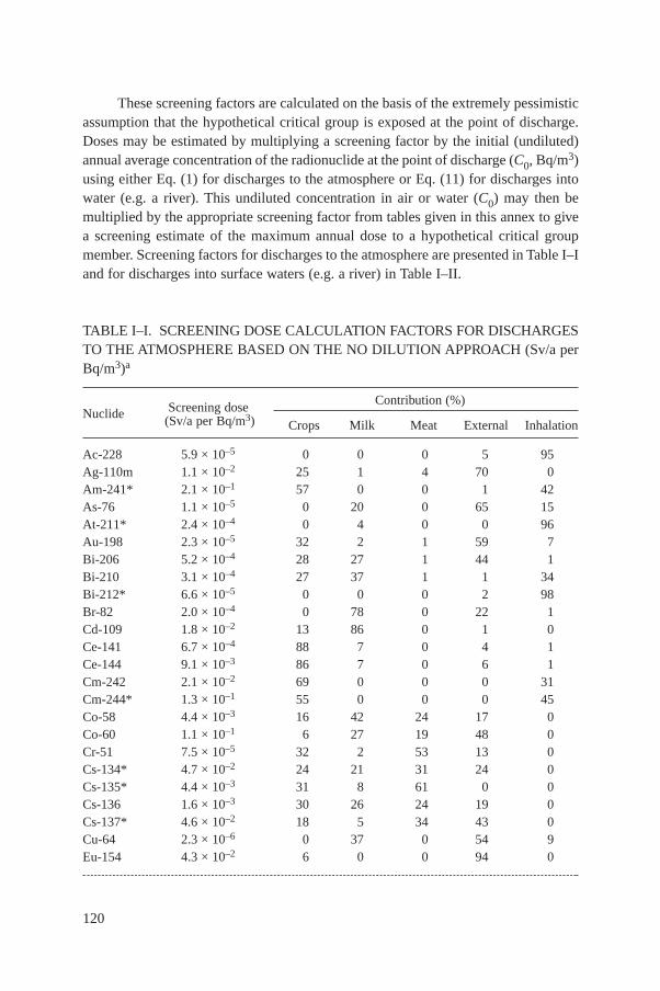
These screening factors are calculated on the basis of the extremely pessimisticassumption that the hypothetical critical group is exposed at the point of discharge.Doses may be estimated by multiplying a screening factor by the initial (undiluted)annual average concentration of the radionuclide at the point of discharge (C0, Bq/m3)using either Eq. (1) for discharges to the atmosphere or Eq. (11) for discharges intowater (e.g. a river). This undiluted concentration in air or water (C0) may then bemultiplied by the appropriate screening factor from tables given in this annex to givea screening estimate of the maximum annual dose to a hypothetical critical groupmember. Screening factors for discharges to the atmosphere are presented in Table I–Iand for discharges into surface waters (e.g. a river) in Table I–II.

120

TABLE I–I. SCREENING DOSE CALCULATION FACTORS FOR DISCHARGESTO THE ATMOSPHERE BASED ON THE NO DILUTION APPROACH (Sv/a perBq/m3)a

Screening dose Contribution (%)Nuclide (Sv/a per Bq/m3) Crops Milk Meat External Inhalation

Ac-228 5.9 × 10–5 0 0 0 5 95Ag-110m 1.1 × 10–2 25 1 4 70 0Am-241* 2.1 × 10–1 57 0 0 1 42As-76 1.1 × 10–5 0 20 0 65 15At-211* 2.4 × 10–4 0 4 0 0 96Au-198 2.3 × 10–5 32 2 1 59 7Bi-206 5.2 × 10–4 28 27 1 44 1Bi-210 3.1 × 10–4 27 37 1 1 34Bi-212* 6.6 × 10–5 0 0 0 2 98Br-82 2.0 × 10–4 0 78 0 22 1Cd-109 1.8 × 10–2 13 86 0 1 0Ce-141 6.7 × 10–4 88 7 0 4 1Ce-144 9.1 × 10–3 86 7 0 6 1Cm-242 2.1 × 10–2 69 0 0 0 31Cm-244* 1.3 × 10–1 55 0 0 0 45Co-58 4.4 × 10–3 16 42 24 17 0 Co-60 1.1 × 10–1 6 27 19 48 0 Cr-51 7.5 × 10–5 32 2 53 13 0 Cs-134* 4.7 × 10–2 24 21 31 24 0 Cs-135* 4.4 × 10–3 31 8 61 0 0 Cs-136 1.6 × 10–3 30 26 24 19 0 Cs-137* 4.6 × 10–2 18 5 34 43 0 Cu-64 2.3 × 10–6 0 37 0 54 9 Eu-154 4.3 × 10–2 6 0 0 94 0

121

TABLE I–I. (cont.)

Screening dose Contribution (%)Nuclide (Sv/a per Bq/m3) Crops Milk Meat External Inhalation

Eu-155 1.7 × 10–3 27 0 1 70 0 Fe-55 1.2 × 10–3 42 3 55 0 0 Fe-59 4.2 × 10–3 42 3 41 14 0 Ga-67 8.7 × 10–6 30 1 0 65 4 Hg-197 9.1 × 10–6 17 56 1 22 5 Hg-197m 4.8 × 10–6 0 60 0 22 18 Hg-203 2.2 × 10–3 70 10 14 6 0 I-123 1.2 × 10–5 0 88 0 9 2 I-125 4.0 × 10–2 22 56 22 0 0 I-129 2.3 × 10–1 20 53 27 0 0 I-131 3.7 × 10–2 12 80 8 0 0 I-132 3.7 × 10–6 0 0 0 91 9 I-133 6.0 × 10–4 0 98 0 1 1I-134 2.3 × 10–6 0 0 0 94 6 I-135 1.4 × 10–5 0 51 0 39 9 In-111 1.8 × 10–5 12 13 0 73 2 In-113m* 3.4 × 10–7 0 0 0 88 12 Mn-54 3.7 × 10–3 18 2 1 79 0 Mo-99 1.3 × 10–4 3 88 0 7 1 Na-22 3.3 × 10–1 1 70 22 7 0 Na-24 4.4 × 10–4 0 93 0 6 0 Nb-95 6.9 × 10–4 56 0 0 44 0 Ni-59 1.1 × 10–2 2 96 2 0 0 Ni-63 2.6 × 10–2 2 96 2 0 0 Np-237* 1.8 × 10–1 46 0 16 11 27 Np-239 1.1 × 10–5 29 15 1 42 14 P-32 1.1 × 10–2 10 82 8 0 0 Pa-231* 7.4 × 10–1 60 0 0 0 40 Pa-233 7.0 × 10–4 91 0 0 9 1 Pb-210 9.3 × 10–1 91 7 2 0 0 Pd-103 1.0 × 10–4 93 3 0 2 1 Pd-107 1.1 × 10–4 96 3 1 0 1 Pd-109 1.2 × 10–6 0 20 0 22 58 Pm-147 4.3 × 10–4 92 1 5 0 1 Po-210 3.0 53 41 6 0 0 Pu-238* 2.3 × 10–1 58 0 0 0 42 Pu-239* 2.5 × 10–1 58 0 0 0 41 Pu-240* 2.5 × 10–1 58 0 0 0 41 Pu-241* 4.8 × 10–3 59 0 0 1 40

122

TABLE I–I. (cont.)

Screening dose Contribution (%)Nuclide (Sv/a per Bq/m3) Crops Milk Meat External Inhalation

Pu-242* 2.4 × 10–1 58 0 0 0 41 Ra-224 1.1 × 10–2 19 51 1 1 28 Ra-225 1.1 × 10–1 63 25 5 0 7 Ra-226 5.7 × 10–1 47 16 8 27 2 Rb-86 5.6 × 10–2 3 96 1 0 0 Rh-105 6.1 × 10–6 1 67 0 22 10 Rh-107* 2.2 × 10–7 0 0 0 84 16 Ru-103 1.4 × 10–3 43 0 41 15 0 Ru-106 2.4 × 10–2 42 0 52 6 0 S-35 1.1 × 10–2 9 49 42 0 0 Sb-124 4.1 × 10–3 60 4 6 30 0 Sb-125 6.6 × 10–3 19 1 3 77 0 Se-75 9.0 × 10–3 26 7 61 6 0 Sn-113 1.7 × 10–3 53 13 12 21 0 Sr-85 1.4 × 10–3 35 31 8 26 0 Sr-87m* 5.9 × 10–7 0 0 0 92 7 Sr-89 5.5 × 10–3 47 41 11 1 0 Sr-90 1.7 × 10–1 18 60 20 2 0 Tc-99 6.6 × 10–3 53 43 4 0 0 Tc-99m 4.4 × 10–7 0 2 0 91 7 Te-125m 4.0 × 10–3 25 35 39 1 0 Te-127m 1.5 × 10–2 23 34 42 0 0 Te-129m 1.1 × 10–2 26 38 36 0 0 Te-131m 2.0 × 10–4 0 87 0 11 1 Te-132 1.4 × 10–3 5 86 2 7 0 Th-228* 4.9 × 10–1 84 0 0 2 14 Th-230* 3.7 × 10–1 33 0 0 42 24 Th-232* 4.4 × 10–1 30 0 0 48 21 Tl-201 1.6 × 10–5 6 74 1 19 1 Tl-202 3.4 × 10–4 31 40 9 19 0 U-232* 4.3 × 10–1 48 3 4 26 18 U-234* 2.1 × 10–1 15 1 1 74 9 U-235* 6.7 × 10–2 44 3 4 22 27 U-238* 2.2 × 10–1 13 1 1 77 8 Y-87 4.0 × 10–5 19 4 1 74 2 Y-90 3.4 × 10–5 56 22 3 10 9 Y-91 3.4 × 10–3 80 1 17 1 0 Zn-65 3.2 × 10–2 15 28 53 5 0 Zr-95 2.0 × 10–3 44 0 0 55 0

a Infants are the limiting exposure group unless otherwise noted by an asterisk, in which caseadults are the limiting group.

I–2. GENERIC FACTORS (DOSE PER UNIT DISCHARGE)

Generic dose calculation factors, based on the generic environmental modelpresented in this report, are also presented in this annex. These factors take accountof the dispersion of radionuclides in the environment, and are therefore of a lesspessimistic nature than the screening values given above. In deriving these genericfactors care has been taken to ensure that doses to a hypothetical critical group areunlikely to exceed those received by an actual critical group by more than a factor often. The result is that, in reality, these generic factors are still likely to representoverestimates of the doses received. The hypothetical critical group doses from unitdischarges of radionuclides to the atmospheric and surface water environments havebeen calculated using a few standardized assumptions about the discharge conditionsand the location of the critical group. The models and data used in these calculationsare described in detail in the main text. The assumptions applied here are similar to thoseused to calculate clearance levels in Ref. [I–1], and have been described in more detailthere. The main underlying assumptions are summarized here for ease of reference.

I–2.1. Atmospheric discharges

Annual average doses to a member of a hypothetical critical group,corresponding to a continuous discharge of 1 Bq/s over a 30 year period, arepresented in Table I–III. An atmospheric discharge was assumed to occur from a pipewith diameter 0.5 m, located on the side of a building with a cross-sectional area of500 m2. A hypothetical critical group member is assumed to live at a distance of 20 mfrom the source. In terms of atmospheric dispersion, this receptor point is within thecavity zone, as explained in the main text. An annual geometric mean wind speedof 2 m/s was assumed, and the fraction of the year for which the wind blows in thesector of interest was assumed to be 0.25. The average air concentration at 20 mcorresponding to a discharge rate of 1 Bq/s under these dispersion conditions is2 × 10–3 Bq/m3. A mean deposition velocity of 1000 m/d was assumed in order toestimate ground deposition levels. At 20 m the average deposition rate on the groundis 2 Bq·m–2·d–1.

It is assumed that terrestrial foods are produced at a greater distance from thesource; crops from a distance of 100 m, and milk and meat from 800 m. Theselocations are within the wake zone for dispersion purposes, as explained in the maintext. The ground deposition rates for these locations are 1.3 × 10–1 and 7.5 × 10–3

Bq·m–2·d–1, respectively. The exposure pathways considered in these calculations are as follows:

inhalation and external exposure from immersion in the cloud (at 20 m), externalexposure from material deposited on the ground (at 20 m) and ingestion of crops(from 100 m) and milk and meat (from 800 m). Effective doses were calculated for

123

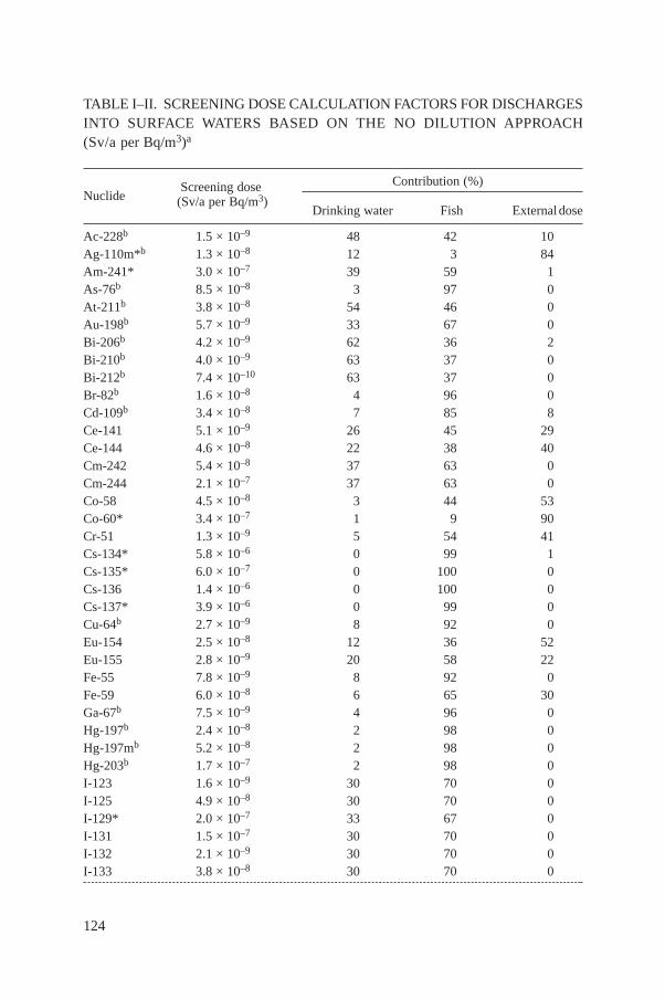
124

TABLE I–II. SCREENING DOSE CALCULATION FACTORS FOR DISCHARGESINTO SURFACE WATERS BASED ON THE NO DILUTION APPROACH(Sv/a per Bq/m3)a

Screening dose Contribution (%)Nuclide (Sv/a per Bq/m3)

Drinking water Fish Externaldose

Ac-228b 1.5 × 10–9 48 42 10Ag-110m*b 1.3 × 10–8 12 3 84Am-241* 3.0 × 10–7 39 59 1As-76b 8.5 × 10–8 3 97 0At-211b 3.8 × 10–8 54 46 0Au-198b 5.7 × 10–9 33 67 0Bi-206b 4.2 × 10–9 62 36 2Bi-210b 4.0 × 10–9 63 37 0Bi-212b 7.4 × 10–10 63 37 0Br-82b 1.6 × 10–8 4 96 0Cd-109b 3.4 × 10–8 7 85 8Ce-141 5.1 × 10–9 26 45 29Ce-144 4.6 × 10–8 22 38 40Cm-242 5.4 × 10–8 37 63 0Cm-244 2.1 × 10–7 37 63 0Co-58 4.5 × 10–8 3 44 53Co-60* 3.4 × 10–7 1 9 90Cr-51 1.3 × 10–9 5 54 41Cs-134* 5.8 × 10–6 0 99 1Cs-135* 6.0 × 10–7 0 100 0Cs-136 1.4 × 10–6 0 100 0Cs-137* 3.9 × 10–6 0 99 0Cu-64b 2.7 × 10–9 8 92 0Eu-154 2.5 × 10–8 12 36 52Eu-155 2.8 × 10–9 20 58 22Fe-55 7.8 × 10–9 8 92 0Fe-59 6.0 × 10–8 6 65 30Ga-67b 7.5 × 10–9 4 96 0Hg-197b 2.4 × 10–8 2 98 0Hg-197mb 5.2 × 10–8 2 98 0Hg-203b 1.7 × 10–7 2 98 0I-123 1.6 × 10–9 30 70 0I-125 4.9 × 10–8 30 70 0I-129* 2.0 × 10–7 33 67 0I-131 1.5 × 10–7 30 70 0I-132 2.1 × 10–9 30 70 0I-133 3.8 × 10–8 30 70 0

125

TABLE I–II. (cont.)

Screening dose Contribution (%)Nuclide (Sv/a per Bq/m3) Drinking water Fish Externaldose

I-134 6.5 × 10–10 30 70 0I-135 7.7 × 10–9 30 70 0In-111b 2.6 × 10–7 0 100 0In-113mb 2.7 × 10–8 0 100 0Mn-54 3.2 × 10–8 3 59 39Mo-99b 1.9 × 10–9 48 27 25Na-22*b 6.4 × 10–8 3 3 94Na-24b 1.5 × 10–9 40 46 13Nb-95*b 7.7 × 10–8 0 7 93Ni-59b 6.0 × 10–10 15 85 0Ni-63b 1.5 × 10–9 15 85 0Np-237* 1.7 × 10–7 40 60 0Np-239 4.0 × 10–9 37 63 0P-32 1.4 × 10–5 0 100 0Pa-231*b 6.4 × 10–7 66 33 1Pa-233*b 4.5 × 10–9 36 21 43Pb-210b 1.7 × 10–5 5 95 0Pd-103b 7.0 × 10–10 52 30 19Pd-107b 1.1 × 10–10 63 37 0Pd-109b 1.7 × 10–9 63 36 1Pm-147 1.4 × 10–9 37 63 0Po-210b 8.9 × 10–6 26 74 0Pu-238* 3.5 × 10–7 40 60 0Pu-239* 3.8 × 10–7 40 60 0Pu-240* 3.8 × 10–7 40 60 0Pu-241* 7.7 × 10–9 37 56 7Pu-242* 3.6 × 10–7 40 60 0Ra-224 6.7 × 10–7 26 74 0Ra-225 1.2 × 10–6 26 74 0Ra-226 9.9 × 10–7 25 73 2Rb-86b 6.1 × 10–7 1 99 0 Rh-105b 1.1 × 10–9 61 35 4 Rh-107b 6.8 × 10–11 62 36 3 Ru-103 2.7 × 10–9 44 26 30 Ru-106 2.3 × 10–8 56 32 12 S-35b 6.6 × 10–8 2 98 0 Sb-124 2.9 × 10–8 15 84 2 Sb-125 1.1 × 10–8 14 82 4 Se-75b 4.2 × 10–8 8 92 0

126

both adults and infants. The dose to the age group receiving the higher dose ispresented in Table I–III. The habit assumptions used in these calculations are given inTable XIV and the effective dose coefficients for external and internal doses are givenin Tables XV–XVII.

TABLE I–II. (cont.)

Screening dose Contribution (%)Nuclide (Sv/a per Bq/m3)

Drinking water Fish Externaldose

Sn-113b 8.9 × 10–9 15 84 1 Sr-85 7.0 × 10–9 11 50 39 Sr-87m 2.4 × 10–10 19 80 1 Sr-89 2.5 × 10–8 19 80 1Sr-90 1.0 × 10–7 18 79 2Tc-99 2.7 × 10–9 46 54 0Tc-99m 7.3 × 10–11 46 54 0Te-125mb 3.9 × 10–8 4 96 0Te-127mb 1.1 × 10–7 4 96 0Te-129mb 1.5 × 10–7 4 96 0Te-131mb 8.8 × 10–8 4 96 0Te-132b 1.9 × 10–7 4 96 0Th-228* 2.9 × 10–6 15 75 10Th-230* 1.2 × 10–6 11 54 35Th-232* 1.4 × 10–6 10 50 40Tl-201b 8.6 × 10–9 2 96 2Tl-202b 3.5 × 10–8 2 89 10U-232 3.4 × 10–7 63 36 0U-234 5.5 × 10–8 61 35 4U-235 5.3 × 10–8 63 36 0U-238 5.1 × 10–8 61 35 4Y-87b 3.0 × 10–9 27 47 25Y-90b 1.4 × 10–8 36 63 1Y-91b 1.4 × 10–8 33 58 9Zn-65 2.5 × 10–7 2 97 2Zr-95 3.5 × 10–8 4 73 23

a Infants are the limiting exposure group unless otherwise noted by an asterisk, in which caseadults are the limiting group.

b Indicates those radionuclides for which Kd values are not available and for which Kdestimates have been made on the basis of chemical similarities.

127

TABLE I–III. DOSE CALCULATION FACTORS FOR DISCHARGES TO THEATMOSPHERE BASED ON THE GENERIC ENVIRONMENTAL MODEL(Sv/a per Bq/s)a

Generic dose factorContribution (%)

Nuclide (Sv/a per Bq/s)Crops Milk Meat External Inhalation

Ac-228 4.7 × 10–7 0 0 0 5 95Ag-110m 6.3 × 10–5 2 0 0 98 0Am-241* 7.9 × 10–4 8 0 0 2 90As-76 6.9 × 10–8 0 0 0 81 19At-211* 1.8 × 10–6 0 0 0 0 100Au-198 1.2 × 10–7 3 0 0 87 10Bi-206 1.9 × 10–6 4 0 0 95 1Bi-210* 1.6 × 10–6 1 0 0 1 98Bi-212* 5.3 × 10–7 0 0 0 2 98Br-82 3.7 × 10–7 0 1 0 96 2Cd-109 2.8 × 10–6 44 17 0 35 4Ce-141 5.6 × 10–7 54 0 0 39 6Ce-144 9.3 × 10–6 44 0 0 51 5Cm-242* 9.1 × 10–5 4 0 0 0 96Cm-244* 4.9 × 10–4 7 0 0 0 92Co-58 6.7 × 10–6 6 1 0 93 0Co-60 4.1 × 10–4 1 0 0 99 0Cr-51 9.3 × 10–8 13 0 1 85 1Cs-134* 9.8 × 10–5 6 0 0 93 0Cs-135* 8.2 × 10–7 86 1 10 2 1Cs-136 2.8 × 10–6 9 0 0 89 1Cs-137* 1.6 × 10–4 3 0 0 97 0Cu-64* 1.2 × 10–8 0 0 0 83 17Eu-154 3.2 × 10–4 0 0 0 99 0Eu-155 1.0 × 10–5 2 0 0 97 1Fe-55 2.9 × 10–7 90 0 7 0 3Fe-59 5.6 × 10–6 16 0 1 82 1Ga-67* 5.0 × 10–8 1 0 0 91 8Hg-197* 2.1 × 10–8 1 0 0 75 24Hg-197m* 1.7 × 10–8 0 0 0 48 52Hg-203 1.8 × 10–6 44 0 1 54 1I-123 1.1 × 10–8 0 3 0 78 19I-125 5.7 × 10–6 79 12 5 4 1I-129* 3.9 × 10–5 86 4 6 3 2I-131 3.8 × 10–6 61 24 2 7 5I-132 3.0 × 10–8 0 0 0 91 9

128

TABLE I–III. (cont.)

Generic dose factor Contribution (%)

Nuclide (Sv/a per Bq/m3) Crops Milk Meat External Inhalation

I-133 1.2 × 10–7 0 15 0 44 42I-134 1.8 × 10–8 0 0 0 94 6I-135 5.4 × 10–8 0 0 0 80 19In-111 1.1 × 10–7 1 0 0 96 3In-113m* 2.7 × 10–9 0 0 0 88 12Mn-54 2.4 × 10–5 1 0 0 98 0Mo-99 9.3 × 10–8 2 4 0 80 14Na-22 1.9 × 10–4 1 4 1 94 0Na-24 2.4 × 10–7 0 5 0 93 2Nb-95 2.6 × 10–6 8 0 0 92 1Ni-59 4.5 × 10–7 27 71 2 0 1Ni-63 1.0 × 10–6 27 71 2 0 1Np-237* 5.9 × 10–4 7 0 0 27 66Np-239 4.9 × 10–8 3 0 0 73 24P-32 1.0 × 10–6 56 27 3 11 4Pa-231* 2.6 × 10–3 9 0 0 1 90Pa-233 8.5 × 10–7 39 0 0 57 4Pb-210 4.7 × 10–4 94 0 0 4 2Pd-103 7.6 × 10–8 67 0 0 26 7Pd-107 6.0 × 10–8 90 0 0 0 9Pd-109* 8.3 × 10–9 0 0 0 25 75Pm-147 2.6 × 10–7 79 0 0 1 19Po-210 9.0 × 10–4 94 4 1 0 1Pu-238* 8.4 × 10–4 8 0 0 0 92Pu-239* 9.2 × 10–4 8 0 0 0 92Pu-240* 9.2 × 10–4 8 0 0 0 92Pu-241* 1.7 × 10–5 9 0 0 2 89Pu-242* 8.8 × 10–4 8 0 0 0 92Ra-224* 5.8 × 10–5 1 0 0 1 99Ra-225* 1.4 × 10–4 6 0 0 0 94Ra-226* 1.5 × 10–3 7 0 0 82 11Rb-86 2.7 × 10–6 29 58 1 11 1Rh-105* 1.7 × 10–8 0 0 0 64 35Rh-107* 1.7 × 10–9 0 0 0 84 16Ru-103 2.0 × 10–6 15 0 1 83 1Ru-106 1.8 × 10–5 29 0 2 65 4S-35 8.1 × 10–7 62 20 17 0 2Sb-124 1.1 × 10–5 11 0 0 88 1Sb-125 4.1 × 10–5 2 0 0 98 0

129

TABLE I–III. (cont.)

Generic dose factor Contribution (%)

Nuclide (Sv/a per Bq/m3) Crops Milk Meat External Inhalation

Se-75 5.6 × 10–6 22 0 3 74 0Sn-113 3.4 × 10–6 14 0 0 85 1Sr-85 3.2 × 10–6 8 0 0 91 0Sr-87m* 4.7 × 10–9 0 0 0 93 7Sr-89 1.8 × 10-6 74 4 1 17 5Sr-90* 5.1 × 10–5 31 2 2 60 5Tc-99 1.9 × 10–6 95 4 0 0 0Tc-99m 3.4 × 10–9 0 0 0 93 7Te-125m 8.2 × 10–7 64 5 6 24 1Te-127m 2.5 × 10–6 75 6 8 9 2Te-129m 2.0 × 10–6 76 6 6 9 2Te-131m 2.1 × 10–7 0 2 0 87 10Te-132 8.7 × 10–7 4 4 0 86 6Th-228* 8.4 × 10–4 25 0 0 11 64Th-230* 2.0 × 10–3 3 0 0 61 36Th-232* 2.5 × 10–3 3 0 0 67 30Tl-201 2.6 × 10–8 2 1 0 93 3Tl-202 5.8 × 10–7 9 1 0 89 1U-232* 1.6 × 10–3 7 0 0 55 38U-234* 1.4 × 10–3 1 0 0 88 11U-235* 2.8 × 10–4 6 0 0 43 52U-238* 1.5 × 10–3 1 0 0 90 9Y-87 2.5 × 10–7 2 0 0 96 3Y-90 6.2 × 10–8 16 0 0 44 40Y-91 1.9 × 10–6 73 0 1 21 5Zn-65 1.6 × 10–5 16 2 3 79 0Zr-95 9.1 × 10–6 5 0 0 94 1

a Infants are the limiting exposure group unless otherwise noted by an asterisk, in which caseadults are the limiting group.

I–2.2. Liquid discharges

Two discharge conditions were considered: the discharge of material into asewerage system and directly into a river. Hypothetical critical group2 annual averagedoses from a unit discharge rate from each mode of discharge are presented inTables I–IV and I–V. The assumptions made in each case are described in turn.

I–2.2.1. Discharge into a sewerage system

In this scenario material is assumed to be discharged into the sewerage systemat a rate of 1 Bq/a and retained in the sewage sludge. The maximum annual averageactivity concentration in sludge was calculated by assuming an annual sewageproduction of 400 t/a (dry weight) as 2.5 × 10–6 Bq/kg per Bq/a discharged.

Two exposure pathways were considered, both of which arise within the sewageplant itself — external irradiation from radionuclides in the sludge and inhalation ofradionuclides resuspended into the air from the sludge.

The hypothetical maximum annual external dose from radionuclides at thesurface of a container full of sewage sludge was calculated. The maximum annualsurface activity concentration was estimated from the total sludge concentration byassuming a density of 1 × 103 kg/m3 and a sludge container depth of 1 m. Workerswithin a sewage plant were assumed to be exposed for a working year of 2000 h/a (or0.288 of the year). The annual dose factors for external dose from surface deposits,given in Table XV, were used to calculate external dose.

Maximum committed effective doses from inhalation of resuspended particlesduring the working year were calculated using the dose coefficients for inhalation (foradults) given in Table XVI. An occupancy factor of 0.288 was applied, as explainedabove. An ambient dust loading of 1 × 10–7 kg/m3 was assumed as described inRef. [I–1]. An average adult inhalation rate of 8400 m3/a, given in Table XIV, wasused to estimate the inhalation dose.

The maximum annual committed effective inhalation and external dosesresulting from an annual discharge into the sewerage system were summed for eachradionuclide and are presented in Table I–IV.

130

2 The doses calculated for discharges into the sewerage system are those to a hypotheticalperson working in the sewerage plant. As such, they are intended to represent the maximum doselikely to be experienced as a result of the discharge.

TABLE I–IV. DOSE CALCULATION FACTORS FOR DISCHARGES INTO ASEWER BASED ON THE GENERIC ENVIRONMENTAL MODEL (Sv/a per Bq/a)a

Nuclide Total dose Contribution (%)(Sv/a per Bq/a) External Inhalation

Ac-228 8.8 × 10–13 100 0Ag-110m 2.4 × 10–12 100 0Am-241 2.6 × 10–14 96 4As-76 4.9 × 10–13 100 0At-211 3.7 × 10–14 100 0Au-198 3.8 × 10–13 100 0Bi-206 2.9 × 10–12 100 0Bi-210 3.2 × 10–14 100 0Bi-212 1.2 × 10–12 100 0Br-82 2.3 × 10–12 100 0Cd-109 2.1 × 10–14 100 0Ce-141 6.8 × 10–14 100 0Ce-144 1.6 × 10–13 100 0Cm-242 1.1 × 10–15 88 12Cm-244 1.5 × 10–15 57 43Co-58 8.6 × 10–13 100 0Co-60 2.1 × 10–12 100 0Cr-51 2.8 × 10–14 100 0Cs-134 1.4 × 10–12 100 0Cs-135 3.1 × 10–17 100 0Cs-136 1.9 × 10–12 100 0Cs-137 5.1 × 10–13 100 0Cu-64 1.7 × 10–13 100 0Eu-154 1.1 × 10–12 100 0Eu-155 5.4 × 10–14 100 0Fe-55 1.8 × 10–20 0 100Fe-59 1.0 × 10–12 100 0Ga-67 1.4 × 10–13 100 0Hg-197 5.9 × 10–14 100 0Hg-197m 7.9 × 10–14 100 0Hg-203 2.1 × 10–13 100 0I-123 1.5 × 10–13 100 0I-125 3.9 × 10–14 100 0I-129 2.4 × 10–14 100 0I-131 3.4 × 10–13 100 0I-132 2.1 × 10–12 100 0I-133 5.8 × 10–13 100 0I-134 2.4 × 10–12 100 0I-135 1.4 × 10–12 100 0

131

TABLE I–IV. (cont.)

Nuclide Total dose Contribution (%)(Sv/a per Bq/a) External Inhalation

In-111 3.6 × 10–13 100 0In-113m 2.3 × 10–13 100 0Mn-54 7.4 × 10–13 100 0Mo-99 2.6 × 10–13 100 0Na-22 1.9 × 10–12 100 0Na-24 3.3 × 10–12 100 0Nb-95 6.8 × 10–13 100 0Ni-59 4.3 × 10–21 0 100Ni-63 1.1 × 10–20 0 100Np-237 2.0 × 10–13 100 0Np-239 1.5 × 10–13 100 0P-32 7.7 × 10–14 100 0Pa-231 4.1 × 10–14 92 8Pa-233 1.8 × 10–13 100 0Pb-210 3.4 × 10–14 100 0Pd-103 1.2 × 10–14 100 0Pd-107 1.4 × 10–20 0 100Pd-109 3.6 × 10–14 100 0Pm-147 3.2 × 10–17 100 0Po-210 2.2 × 10–17 34 66Pu-238 1.9 × 10–15 43 57Pu-239 1.6 × 10–15 23 77Pu-240 2.0 × 10–15 40 60Pu-241 8.7 × 10–16 98 2Pu-242 1.8 × 10–15 37 63Ra-224 1.3 × 10–12 100 0Ra-225 2.5 × 10–13 100 0Ra-226 1.6 × 10–12 100 0Rb-86 1.5 × 10–13 100 0Rh-105 7.0 × 10–14 100 0Rh-107 3.2 × 10–13 100 0Ru-103 4.2 × 10–13 100 0Ru-106 3.2 × 10–13 100 0S-35 1.6 × 10–17 100 0Sb-124 1.6 × 10–12 100 0Sb-125 3.9 × 10–13 100 0Se-75 3.4 × 10–13 100 0Sn-113 2.5 × 10–13 100 0Sr-85 4.6 × 10–13 100 0Sr-87m 2.9 × 10–13 100 0

132

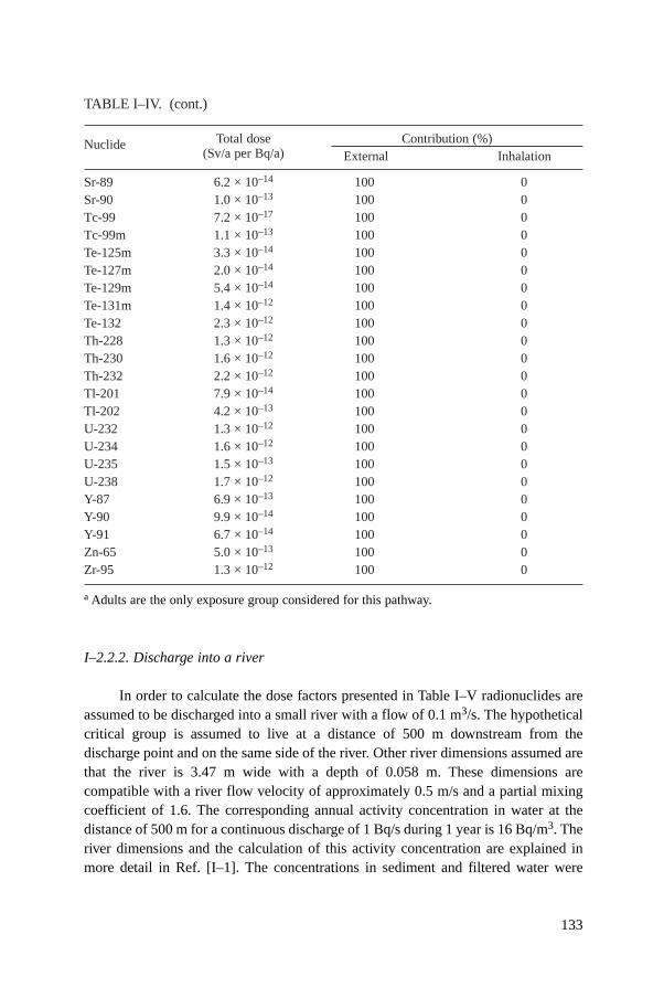
TABLE I–IV. (cont.)

Nuclide Total dose Contribution (%)(Sv/a per Bq/a) External Inhalation

Sr-89 6.2 × 10–14 100 0Sr-90 1.0 × 10–13 100 0Tc-99 7.2 × 10–17 100 0Tc-99m 1.1 × 10–13 100 0Te-125m 3.3 × 10–14 100 0Te-127m 2.0 × 10–14 100 0Te-129m 5.4 × 10–14 100 0Te-131m 1.4 × 10–12 100 0Te-132 2.3 × 10–12 100 0Th-228 1.3 × 10–12 100 0Th-230 1.6 × 10–12 100 0Th-232 2.2 × 10–12 100 0Tl-201 7.9 × 10–14 100 0Tl-202 4.2 × 10–13 100 0U-232 1.3 × 10–12 100 0U-234 1.6 × 10–12 100 0U-235 1.5 × 10–13 100 0U-238 1.7 × 10–12 100 0Y-87 6.9 × 10–13 100 0Y-90 9.9 × 10–14 100 0Y-91 6.7 × 10–14 100 0Zn-65 5.0 × 10–13 100 0Zr-95 1.3 × 10–12 100 0

a Adults are the only exposure group considered for this pathway.

I–2.2.2. Discharge into a river

In order to calculate the dose factors presented in Table I–V radionuclides areassumed to be discharged into a small river with a flow of 0.1 m3/s. The hypotheticalcritical group is assumed to live at a distance of 500 m downstream from thedischarge point and on the same side of the river. Other river dimensions assumed arethat the river is 3.47 m wide with a depth of 0.058 m. These dimensions arecompatible with a river flow velocity of approximately 0.5 m/s and a partial mixingcoefficient of 1.6. The corresponding annual activity concentration in water at thedistance of 500 m for a continuous discharge of 1 Bq/s during 1 year is 16 Bq/m3. Theriver dimensions and the calculation of this activity concentration are explained inmore detail in Ref. [I–1]. The concentrations in sediment and filtered water were

133

TABLE I–V. DOSE CALCULATION FACTORS FOR DISCHARGES INTOSURFACE WATER BASED ON THE GENERIC ENVIRONMENTAL MODEL(Sv/a per Bq/s)a

Nuclide Generic dose factor Contribution (%)Sv/a per Bq/s Drinking water Fish External

Ac-228b 2.3 × 10–8 48 42 10Ag-110m*b 2.2 × 10–7 38 29 33Am-241* 4.9 × 10–6 12 6 82As-76b 1.4 × 10–6 3 97 0At-211b 5.9 × 10–7 54 46 0Au-198b 9.0 × 10–8 33 67 0Bi-206b 6.7 × 10–8 62 36 2Bi-210b 6.4 × 10–8 63 37 0Bi-212b 9.8 × 10–9 63 37 0Br-82b 2.6 × 10–7 4 96 0Cd-109b 5.4 × 10–7 7 85 8Ce-141 8.1 × 10–8 26 45 29Ce-144 7.3 × 10–7 22 38 40Cm-242 8.6 × 10–7 37 63 0Cm-244 3.3 × 10–6 37 63 0Co-58 7.2 × 10–7 3 44 53Co-60* 5.4 × 10–6 1 9 90Cr-51 2.0 × 10–8 5 54 41Cs-134* 9.2 × 10–5 0 99 1Cs-135* 9.6 × 10–6 0 100 0Cs-136 2.3 × 10–5 0 100 0Cs-137* 6.3 × 10–5 0 99 0Cu-64b 4.3 × 10–8 8 92 0Eu-154 4.0 × 10–7 12 36 52Eu-155 4.5 × 10–8 20 58 22Fe-55 1.3 × 10–7 8 92 0Fe-59 9.7 × 10–7 6 65 30Ga-67b 1.2 × 10–7 4 96 0Hg-197b 3.9 × 10–7 2 98 0Hg-197mb 8.2 × 10–7 2 98 0Hg-203b 2.7 × 10–6 2 98 0I-123 2.6 × 10–8 30 70 0I-125 7.8 × 10–7 30 70 0I-129* 3.2 × 10–6 33 67 0I-131 2.5 × 10–6 30 70 0I-132 3.0 × 10–8 30 70 0I-133 6.0 × 10–7 30 70 0I-134 8.3 × 10–9 30 70 0

134

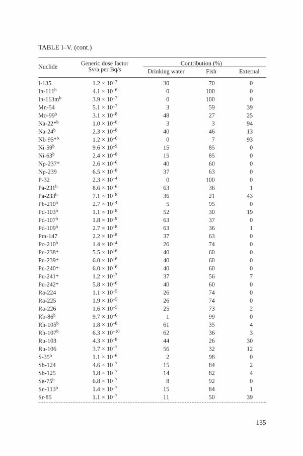
TABLE I–V. (cont.)

Nuclide Generic dose factor Contribution (%)Sv/a per Bq/s Drinking water Fish External

I-135 1.2 × 10–7 30 70 0In-111b 4.1 × 10–6 0 100 0In-113mb 3.9 × 10–7 0 100 0Mn-54 5.1 × 10–7 3 59 39Mo-99b 3.1 × 10–8 48 27 25Na-22*b 1.0 × 10–6 3 3 94Na-24b 2.3 × 10–8 40 46 13Nb-95*b 1.2 × 10–6 0 7 93Ni-59b 9.6 × 10–9 15 85 0Ni-63b 2.4 × 10–8 15 85 0Np-237* 2.6 × 10–6 40 60 0Np-239 6.5 × 10–8 37 63 0P-32 2.3 × 10–4 0 100 0Pa-231b 8.6 × 10–6 63 36 1Pa-233b 7.1 × 10–8 36 21 43Pb-210b 2.7 × 10–4 5 95 0Pd-103b 1.1 × 10–8 52 30 19Pd-107b 1.8 × 10–9 63 37 0Pd-109b 2.7 × 10–8 63 36 1Pm-147 2.2 × 10–8 37 63 0Po-210b 1.4 × 10–4 26 74 0Pu-238* 5.5 × 10–6 40 60 0Pu-239* 6.0 × 10–6 40 60 0Pu-240* 6.0 × 10–6 40 60 0Pu-241* 1.2 × 10–7 37 56 7Pu-242* 5.8 × 10–6 40 60 0Ra-224 1.1 × 10–5 26 74 0Ra-225 1.9 × 10–5 26 74 0Ra-226 1.6 × 10–5 25 73 2Rb-86b 9.7 × 10–6 1 99 0Rh-105b 1.8 × 10–8 61 35 4Rh-107b 6.3 × 10–10 62 36 3Ru-103 4.3 × 10–8 44 26 30Ru-106 3.7 × 10–7 56 32 12S-35b 1.1 × 10–6 2 98 0Sb-124 4.6 × 10–7 15 84 2Sb-125 1.8 × 10–7 14 82 4Se-75b 6.8 × 10–7 8 92 0Sn-113b 1.4 × 10–7 15 84 1Sr-85 1.1 × 10–7 11 50 39

135

136

TABLE I–V. (cont.)

Nuclide Generic dose factor Contribution (%)Sv/a per Bq/s Drinking water Fish External

Sr-87m 3.6 × 10–9 19 80 1Sr-89 4.0 × 10–7 19 80 1Sr-90 1.7 × 10–6 18 79 2Tc-99 4.3 × 10–8 46 54 0Tc-99m 1.1 × 10–9 46 54 0Te-125mb 6.3 × 10–7 4 96 0Te-127mb 1.8 × 10–6 4 96 0Te-129mb 2.4 × 10–6 4 96 0Te-131mb 1.4 × 10–6 4 96 0Te-132b 3.0 × 10–6 4 96 0Th-228* 4.6 × 10–5 15 75 10Th-230* 1.9 × 10–5 11 54 35Th-232* 2.2 × 10–5 10 50 40Tl-201b 1.4 × 10–7 2 96 2Tl-202b 5.7 × 10–7 2 89 10U-232 5.4 × 10–6 63 36 0U-234 8.9 × 10–7 61 35 4U-235 8.6 × 10–7 63 36 0U-238 8.2 × 10–7 61 35 4Y-87b 4.9 × 10–8 27 47 25Y-90b 2.3 × 10–7 36 63 1Y-91b 2.3 × 10–7 33 58 9Zn-65 4.0 × 10–6 2 97 2Zr-95 5.5 × 10–7 4 73 23

a Infants are the limiting exposure group unless otherwise noted by an asterisk, in which caseadults are the limiting group.

b Indicates those radionuclides for which Kd values are not available and for which Kdestimates have been made on the basis of chemical similarities.

calculated using the Kd values for each radionuclide given in Table VI, supplementedby assumptions based on chemical analogy, and a default suspended sedimentfraction of 5 × 10–2 kg/m3 (see Ref. [I–1] for a more detailed explanation).

The following exposure pathways were considered: drinking water, ingestion offreshwater fish and external irradiation from radionuclides in shore/beach sediment.The dose from drinking water was calculated assuming that the water was filteredbefore consumption. The average annual activity concentration in fish was calculated

from the water concentration using the bioaccumulation factors given in Table XIII.The ingestion rates for drinking water and fish were taken from Table XIV and thedose coefficients for ingestion were taken from Table XVII.

The maximum annual surface activity concentration in beach sediment wascalculated from the annual average water concentration and the relevant Kd value andusing a factor of 60 kg/m2 for the top 5 cm and the bulk density of sediments. Aconversion factor of 0.1 was also applied to take account of the fact that the Kd valuefor beach sediment is one tenth of that for suspended sediment. Buildup during oneyear was taken into account, and the dose coefficients for external dose from depositsgiven in Table XV were applied to calculate maximum annual external doses,together with the occupancy factors for each age group presented in Table XIV.

The total dose from the three pathways was estimated for adults and childrenfor each radionuclide. The dose to the age group with the higher dose is presented inTable I–V.

REFERENCE

[I–1] INTERNATIONAL ATOMIC ENERGY AGENCY, Evaluating the Reliability ofPredictions Made Using Environmental Transfer Models, Safety Series No. 100, IAEA,Vienna (1989).

137

Annex II

RADIONUCLIDE HALF-LIVES AND DECAY CONSTANTS

Half-lives (T1/2) and decay constants (li) for the radionuclides of concern areprovided in Table II–I. Values for the half-lives were obtained from Ref. [II–1] andare provided in units of years (a), days (d) and hours (h). Decay constants werecalculated from the half-lives and are provided in units of per day (d–1) and persecond (s–1).

TABLE II–I. RADIONUCLIDE HALF-LIVES AND DECAY CONSTANTS

Nuclide Half-life (T1/2) li (s–1) li (d–1)

Ac-228 6.13 h 3.14 × 10–5 2.71Ag-110m 250 d 3.21 × 10–8 2.77 × 10–3

Am-241 4.32 × 102 a 5.09 × 10–11 4.40 × 10–6

As-76 1.10 d 7.29 × 10–6 6.30 × 10–1

At-211 7.21 h 2.67 × 10–5 2.31Au-198 2.69 d 2.98 × 10–6 2.58 × 10–1

Bi-206 6.24 d 1.29 × 10–6 1.11 × 10–1

Bi-210 5.01 d 1.60 × 10–6 1.38 × 10–1

Bi-212 1.01 h 1.91 × 10–4 1.65 × 101

Br-82 1.47 d 5.46 × 10–6 4.72 × 10–1

Cd-109 1.27 a 1.73 × 10–8 1.50 × 10–3

Ce-141 32.5 d 2.47 × 10–7 2.13 × 10–2

Ce-144 284 d 2.82 × 10–8 2.44 × 10–3

Cm-242 163 d 4.92 × 10–8 4.25 × 10–3

Cm-244 18.1 a 1.21 × 10–9 1.05 × 10–4

Co-58 70.8 d 1.13 × 10–7 9.79 × 10–3

Co-60 5.27 a 4.17 × 10–9 3.60 × 10–4

Cr-51 27.7 d 2.90 × 10–7 2.50 × 10–2

Cs-134 2.06 a 1.07 × 10–8 9.22 × 10–4

Cs-135 2.30 × 106 a 9.56 × 10–15 8.26 × 10–10

Cs-136 13.1 d 6.12 × 10–7 5.29 × 10–2

Cs-137 30.0 a 7.33 × 10–10 6.33 × 10–5

Cu-64 12.7 h 1.52 × 10–5 1.31Eu-154 8.80 a 2.50 × 10–9 2.16 × 10–4

Eu-155 4.96 a 4.43 × 10–9 3.83 × 10–4

Fe-55 2.70 a 8.14 × 10–9 7.03 × 10–4

Fe-59 44.5 d 1.80 × 10–7 1.56 × 10–2

Ga-67 3.26 d 2.46 × 10–6 2.13 × 10–1

Hg-197 2.67 d 3.00 × 10–6 2.60 × 10–1

Hg-197m 23.8 h 8.09 × 10–6 6.99 × 10–1

138

TABLE II–I. (cont.)

Nuclide Half-life (T1/2) li (s–1) li (d–1)

Hg-203 46.6 d 1.72 × 10–7 1.49 × 10–2

I-123 13.2 h 1.46 × 10–5 1.26I-125 60.1 d 1.33 × 10–7 1.15 × 10–2

I-129 1.57 × 107 a 1.40 × 10–15 1.21 × 10–10

I-131 8.04 d 9.98 × 10–7 8.62 × 10–2

I-132 2.30 h 8.37 × 10–5 7.23I-133 20.8 h 9.26 × 10–6 8.00 × 10–1

I-134 0.876 h 2.20 × 10–4 1.90 × 101

I-135 6.61 h 2.91 × 10–5 2.52In-111 2.83 d 2.83 × 10–6 2.45 × 10–1

In-113m 1.66 h 1.16 × 10–4 1.00 × 101

Mn-54 312 d 2.57 × 10–8 2.22 × 10–3

Mo-99 2.75 d 2.92 × 10–6 2.52 × 10–1

Na-22 2.60 a 8.45 × 10–9 7.30 × 10–4

Na-24 15.0 h 1.28 × 10–5 1.11Nb-95 35.1 d 2.29 × 10–7 1.97 × 10–2

Ni-59 7.50 × 104 a 2.93 × 10–13 2.53 × 10–8

Ni-63 96.0 a 2.29 × 10–10 1.98 × 10–5

Np-237 2.14 × 106 a 1.03 × 10–14 8.87 × 10–10

Np-239 2.36 d 3.40 × 10–6 2.94 × 10–1

P-32 14.3 d 5.61 × 10–7 4.85 × 10–2

Pa-231 3.27 × 104 a 6.72 × 10–13 5.81 × 10–8

Pa-233 27.0 d 2.97 × 10–7 2.57 × 10–2

Pb-210 22.3 a 9.86 × 10–10 8.52 × 10–5

Pd-103 17.0 d 4.72 × 10–7 4.08 × 10–2

Pd-107 6.50 × 106 a 3.38 × 10–15 2.92 × 10–10

Pd-109 13.4 h 1.44 × 10–5 1.24Pm-147 2.62 a 8.39 × 10–9 7.25 × 10–4

Po-210 138 d 5.81 × 10–8 5.02 × 10–3

Pu-238 87.7 a 2.51 × 10–10 2.17 × 10–5

Pu-239 2.41 × 104 a 9.12 × 10–13 7.88 × 10–8

Pu-240 6.54 × 103 a 3.36 × 10–12 2.90 × 10–7

Pu-241 14.4 a 1.53 × 10–9 1.32 × 10–4

Pu-242 3.76 × 105 a 5.85 × 10–14 5.05 × 10–9

Ra-224 3.66 d 2.19 × 10–6 1.89 × 10–1

Ra-225 14.8 d 5.42 × 10–7 4.68 × 10–2

Ra-226 1.60 × 103 a 1.37 × 10–11 1.19 × 10–6

Rb-86 18.7 d 4.29 × 10–7 3.71 × 10–2

Rh-105 1.47 d 5.46 × 10–6 4.72 × 10–1

Rh-107 0.362 h 5.32 × 10–4 4.60 × 101

Ru-103 39.3 d 2.04 × 10–7 1.76 × 10–2

139

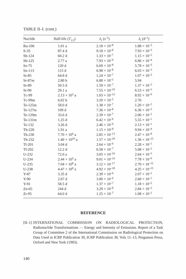
TABLE II–I. (cont.)

Nuclide Half-life (T1/2) li (s–1) li (d–1)

Ru-106 1.01 a 2.18 × 10–8 1.88 × 10–3

S-35 87.4 d 9.18 × 10–8 7.93 × 10–3

Sb-124 60.2 d 1.33 × 10–7 1.15 × 10–2

Sb-125 2.77 a 7.93 × 10–9 6.86 × 10–4

Se-75 120 d 6.69 × 10–8 5.78 × 10–3

Sn-113 115 d 6.98 × 10–8 6.03 × 10–3

Sr-85 64.8 d 1.24 × 10–7 1.07 × 10–2

Sr-87m 2.80 h 6.88 × 10–5 5.94Sr-89 50.5 d 1.59 × 10–7 1.37 × 10–2

Sr-90 29.1 a 7.55 × 10–10 6.53 × 10–5

Tc-99 2.13 × 105 a 1.03 × 10–13 8.92 × 10–9

Tc-99m 6.02 h 3.20 × 10–5 2.76Te-125m 58.0 d 1.38 × 10–7 1.20 × 10–2

Te-127m 109 d 7.36 × 10–8 6.36 × 10–3

Te-129m 33.6 d 2.39 × 10–7 2.06 × 10–2

Te-131m 1.25 d 6.42 × 10–6 5.55 × 10–1

Te-132 3.26 d 2.46 × 10–6 2.13 × 10–1

Th-228 1.91 a 1.15 × 10–8 9.94 × 10–4

Th-230 7.70 × 104 a 2.85 × 10–13 2.47 × 10–8

Th-232 1.40 × 1010 a 1.57 × 10–18 1.36 × 10–13

Tl-201 3.04 d 2.64 × 10–6 2.28 × 10–1

Tl-202 12.2 d 6.58 × 10–7 5.68 × 10–2

U-232 72.0 a 3.05 × 10–10 2.64 × 10–5

U-234 2.44 × 105 a 9.01 × 10–14 7.78 × 10–9

U-235 7.04 × 108 a 3.12 × 10–17 2.70 × 10–12

U-238 4.47 × 109 a 4.92 × 10–18 4.25 × 10–13

Y-87 3.35 d 2.39 × 10–6 2.07 × 10–1

Y-90 2.67 d 3.00 × 10–6 2.60 × 10–1

Y-91 58.5 d 1.37 × 10–7 1.18 × 10–2

Zn-65 244 d 3.29 × 10–8 2.84 × 10–3

Zr-95 64.0 d 1.25 × 10–7 1.08 × 10–2

REFERENCE

[II–1] INTERNATIONAL COMMISSION ON RADIOLOGICAL PROTECTION,Radionuclide Transformations — Energy and Intensity of Emissions. Report of a TaskGroup of Committee 2 of the International Commission on Radiological Protection onData Used in ICRP Publication 30, ICRP Publication 38, Vols 11–13, Pergamon Press,Oxford and New York (1983).

140

141

Annex III

SPECIAL CONSIDERATIONS FOR ASSESSMENT OF DISCHARGES OFTRITIUM AND CARBON-14

Since 3H and 14C can be incorporated into a great variety of different chemicalcompounds within the human body, the radiological dose from releases of theseradionuclides is best assessed using models that employ a specific activity approach[III–1, III–2]. These models are based on the assumption that a steady stateequilibrium has been attained between the environment and the exposed individuals,so that the ratio between the radionuclide and its stable counterpart is fixed. Suchmodels are considered to give conservative dose estimates when an individual isassumed to be in complete equilibrium with maximum levels of environmentalspecific activity of 3H and 14C. However, more advanced models have been developedto assess exposure under non-equilibrium conditions and to include the specialbehaviour of 3H and 14C in organic compounds [III–3]. They indicate that takingaccount of incorporation into organic compounds can lead to estimated doses that arehigher than those obtained using the specific activity model. For simplicity, andtaking account of other conservatisms inherent in the dose calculation, the specificactivity approach is adopted here. More detailed models may be needed if the totaldose to the critical group exceeds the reference level discussed in Sections 2 and 8 andexposure to 3H or 14C is a significant contributor to that dose.

III–1. TRITIUM

The specific activity model for 3H assumes that the nuclide is transferredthrough the environment and incorporated into the organism through its associationwith water molecules. It is also assumed that the concentration of 3H in humans isderived from equilibrium concentrations of 3H in water vapour present in theatmosphere receiving the airborne discharges, and from water of the aquaticenvironments receiving liquid discharges. Thus the dose rate is calculated as follows.

DTmax = [(CA)max

x1¥ ( fA)x1

+ (CW)maxx2

¥ ( fW)x2]g (III–1)

where

DTmax is the dose rate (Sv/a) for 3H to the body of a representative member of

the critical group;

(CA)maxx1

is the steady state concentration of 3H in atmospheric water vapour(Bq/L) at location x1 resulting from airborne releases (this is theatmospheric concentration relevant for calculating critical group doses);

( fA)x1is the fraction of the total water intake that is derived from atmosphericwater vapour at location x1 (this fraction includes water absorbed throughthe skin and through inhalation, as well as water vapour included in theformation of rain that is incorporated into foods and drinking water andother liquids produced at location x1 and subsequently consumed by theindividual);

(CW)maxx2

is the steady state concentration of 3H in water at location x2 resulting fromreleases to the aquatic environment (Bq/L) (this is the concentration inthe aquatic environment relevant for calculating critical group doses);

( fW)x2is the fraction of the total water intake of the potentially exposed personthat is derived from water at location x2 that has been contaminated withaquatic discharges of tritiated water (this fraction includes theconsumption of water in foods that have been irrigated with water fromlocation x2, as well as drinking water and other water based beveragesderived from this location);

g is the dose rate conversion factor (Sv/a per Bq/L of human body watercontent).

The concentration of 3H atmospheric water vapour at location x1 is calculated as

(III–2)

where

(X)maxx1

is the concentration of 3H in air at location x1 (Bq/m3) resulting from arelease to the atmosphere (computations of (X)max

x1are performed using

the equations described in Section 3 of this report),( H)x1

is the absolute humidity of the atmosphere, assumed as a default value tobe 6 × 10–3 L/m3 of air or 6 × 10–3 kg/m3.

The concentration of 3H in water at location x2, resulting from discharges of 3Hto the aquatic environment (CW)x1

, may be estimated using the models described inSection 4.

For the parameters (fA)x1and (fA)x2

default values of unity are proposed. Thisvalue of unity results in a sufficiently cautious estimate of dose rates, given accurateestimates of the maximum specific activity of 3H at locations x1 and x2.

max

max 1

11

( )( )

( )

x

A xx

XC

H=

142

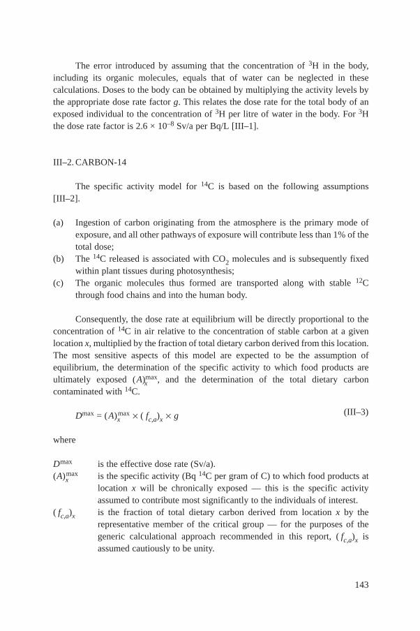
The error introduced by assuming that the concentration of 3H in the body,including its organic molecules, equals that of water can be neglected in thesecalculations. Doses to the body can be obtained by multiplying the activity levels bythe appropriate dose rate factor g. This relates the dose rate for the total body of anexposed individual to the concentration of 3H per litre of water in the body. For 3Hthe dose rate factor is 2.6 × 10–8 Sv/a per Bq/L [III–1].

III–2. CARBON-14

The specific activity model for 14C is based on the following assumptions[III–2].

(a) Ingestion of carbon originating from the atmosphere is the primary mode ofexposure, and all other pathways of exposure will contribute less than 1% of thetotal dose;

(b) The 14C released is associated with CO2 molecules and is subsequently fixedwithin plant tissues during photosynthesis;

(c) The organic molecules thus formed are transported along with stable 12Cthrough food chains and into the human body.

Consequently, the dose rate at equilibrium will be directly proportional to theconcentration of 14C in air relative to the concentration of stable carbon at a givenlocation x, multiplied by the fraction of total dietary carbon derived from this location.The most sensitive aspects of this model are expected to be the assumption ofequilibrium, the determination of the specific activity to which food products areultimately exposed (A)x

max, and the determination of the total dietary carboncontaminated with 14C.

Dmax = (A)xmax ¥ ( fc,a)x ¥ g (III–3)

where

Dmax is the effective dose rate (Sv/a).(A)x

max is the specific activity (Bq 14C per gram of C) to which food products atlocation x will be chronically exposed — this is the specific activityassumed to contribute most significantly to the individuals of interest.

( fc,a)x is the fraction of total dietary carbon derived from location x by therepresentative member of the critical group — for the purposes of thegeneric calculational approach recommended in this report, ( fc,a)x isassumed cautiously to be unity.

143

g is the effective dose rate factor that relates the annual dose rate (Sv/a) to theconcentration of 14C per gram of carbon in people (Bq/g). The dose ratefactor recommended for screening is 5.6 × 10–5 Sv/a per Bq/g [III–2].

Values of (A)xmax can be calculated as follows.

(III–4)

where

(X)xmax is the concentration of 14C in air at location x (Bq/m3) calculated using

the equations described in Section 3 of this report;(C)x is the concentration of airborne carbon, assumed to be 1.8 × 10–1 g/m3,

corresponding to an average atmospheric CO2 concentration of 330 ppm(vol.).

REFERENCES

[III–1] INTERNATIONAL COMMISSION ON RADIOLOGICAL PROTECTION,Age-dependent Doses to Members of the Public from Intake of Radionuclides, Part 5,Compilation of Ingestion and Inhalation Dose Coefficients, ICRP Publication No. 72,Pergamon Press, Oxford and New York (1996).

[III–2] KILLOUGH, G.G., ROHWER, P.S., A new look at the dosimetry of 14C released to theatmosphere as carbon dioxide, Health Phys. 34 (1978) 141–159.

[III–3] GALERIU, D., Transfer Parameters for Routine Releases of HTO — Consideration ofOBT, Rep. AECL-11052, COG-94-76, Atomic Energy of Canada, Chalk River, ON(1994).

( )( )

( )max

max

AX

Cxx

x

=

144

145

Annex IV

EXAMPLE CALCULATIONS

IV–1. EXAMPLE CALCULATION FOR DISCHARGES TO THE ATMOSPHEREWHEN H > 2.5HB

IV–1.1. Scenario description

Iodine-131 is released at an average rate Qi = 1 Bq/s from a stack with heightH = 60 m. The nearest building with a potential for influencing the flow of this plumehas a height HB = 20 m. A farm is located 1 km downwind of this release point.Assuming that an individual lives an entire year at this farm, what is the annualaverage air concentration and the ground deposition rate at this location?

IV–1.2. Calculational procedure

The first step is to determine which dispersion model is most appropriate. Inthis case 2.5HB = (2.5) (20) m = 50 m. Thus H > 2.5HB, and since x < 20 m, Eq. (2)should be used in this calculation

CA = (Pp)(F)(Qi)/ua

In the absence of site specific information, use the default values Pp = 0.25 andua = 2 m/s. From Table I for H = 46–80 m and x = 1000 m,F = 1 × 10–5 m–2.Substituting into Eq. (2) gives

CA = (0.25)(1 × 10–5 m–2)(1 Bq/s)/(2 m/s)–1

= 1.3 × 10–6 Bq/m3

The deposition rate for this location is given by the equation

d⋅ i = (VT)(CA)

(Section 3.9). Use of the default value of VT = 1000 m/d for 131I gives

d⋅ i = (1000 m/d)(1.3× 10–6 Bq/m3)= 1.3 × 10–3 Bq·m–2·d–1

IV–2. EXAMPLE CALCULATION FOR DISCHARGES TO THE ATMOSPHEREFOR RECEPTORS IN THE WAKE AND CAVITY ZONES

IV–2.1. Scenario description

Assume the same information as in Example IV–1, except that the radioactivematerial is being released to the atmosphere from a small vent pipe in the side of abuilding. The diameter of the vent pipe is 0.5 m and the cross-sectional area of thebuilding AB is 500 m2. On the same side of the building, 5 m from the release point,is located the air intake for a private residence. An individual resides in that locationat all times. Further, all of this person’s food is provided by a farm located 1 kmdownwind of this release point. What are the annual average air concentration andground deposition rates at these two locations?

IV–2.2. Calculational procedure

IV–2.2.1. Residence

Since the source and receptor are located on the same building surface, theprocedures outlined in Section 3.6.1 should be used. The concentration in air may becalculated using Eq. (7) since x (5 m) is greater than three times the diameter of thevent stack (3 × 0.5 m = 1.5 m).

CA = (B0)(Qi)/(ua)(x2)

Using the parameter values appropriate for this problem

CA = (30)(1 Bq/s)/(2 m/s)(5 m)2

= 0.6 Bq/m3

Again, using Section 3.9 to calculate the ground deposition rate

d⋅ i = (1000 m/d)(0.6 Bq/m3)= 600 Bq·m–2 ·d–1

IV–2.2.2. Farm

Since 2.5 times the square root of the cross-sectional area of this building is56 m, which is less than the downwind distance to the farm of 1 km, Eq. (4) inSection 3.5 is appropriate.

146

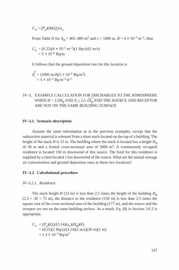
CA = (Pp)(B)(Qi)/ua

From Table II for AB = 401–800 m2 and x = 1000 m, B = 4 × 10–5 m–2; thus

CA = (0.25)(4 × 10–5 m–2)(1 Bq/s)/(2 m/s)= 5 × 10–6 Bq/m

It follows that the ground deposition rate for this location is

d⋅ i = (1000 m/d)(5 × 10–6 Bq/m3)= 5 × 10–3 Bq·m–2·d–1

IV–3. EXAMPLE CALCULATION FOR DISCHARGES TO THE ATMOSPHEREWHEN H < 2.5HB AND X < 2.5 √AB AND THE SOURCE AND RECEPTOR ARE NOT ON THE SAME BUILDING SURFACE

IV–3.1. Scenario description

Assume the same information as in the previous examples, except that theradioactive material is released from a short stack located on the top of a building. Theheight of the stack H is 33 m. The building where the stack is located has a height HBof 30 m and a frontal cross-sectional area of 5000 m2. A continuously occupiedresidence is located 150 m downwind of this source. The food for this residence issupplied by a farm located 1 km downwind of the source. What are the annual averageair concentration and ground deposition rates at these two locations?

IV–3.2. Calculational procedure

IV–3.2.1. Residence

The stack height H (33 m) is less than 2.5 times the height of the building HB(2.5 × 30 = 75 m), the distance to the residence (150 m) is less than 2.5 times thesquare root of the cross-sectional area of the building (177 m), and the source and thereceptor are not on the same building surface. As a result, Eq. (8) in Section 3.6.2 isappropriate.

CA = (Pp)(Qi)/(3.14)(ua)(HB)(K)= (0.25)(1 Bq/s)/(3.14)(2 m/s)(30 m)(1 m)= 1.3 × 10–3 Bq/m3

147

The ground deposition rate at this location is again given by

d⋅ i = (1000 m/d)(1.3 × 10–3 Bq/m3)= 1.3 Bq·m–2·d–1

IV–3.2.2. Farm

Since the downwind distance to the farm (1000 m) is greater than 2.5 times thesquare root of the frontal cross-sectional area, this problem is identical to the farmportion of Example IV–2; that is

CA = 5 × 10–6 Bq/m3

d⋅ i = 5 × 10–3 Bq·m–2·d–1

IV–4. EXAMPLE CALCULATION FOR DISCHARGES INTO A RIVER

IV–4.1. Scenario description

Caesium-137 is to be released to a relatively small river at a release rate of3.7 × 1010 Bq/a with a radionuclide effluent discharge rate of 1 m3/s. A 30 year lowannual riverflow rate is not known, but a representative river width under normal(mean annual) river discharge conditions is estimated to be 50 m. The nearestpotentially exposed individual lives 1 km downstream from the outfall on the sameside of the river. Determine the 137Cs concentration 1 km downstream.

IV–4.2. Calculational procedure

Qi = 3.7 × 1010 Bq/a = 1170 Bq/s

F = 1 m3/s

λi = 7.33 × 10–10 s–1 (from Annex II)

B = 50 m,x = 1000 m

The river conditions under a 30 year low annual mean flow must first beestimated. From Table III B = 50 m corresponds to a mean annual river flow rate ofaround ¯qr = 30 m3/s. Thus the 30 year low annual riverflow rate qr = qr /3 = 10 m3/s.

From Table III qr = 10 m3/s gives B = 28.8 m and D = 0.48 m, and since U =qr /BD, U = 0.72 m/s. Lz = 7 × D = 3.4 m,x = 1000 > Lz , so correction for partialmixing is required.

148

A = 1.5Dx /B2 = 0.87

From Table IV the river partial mixing correction factor (Pr) corresponding toA = 0.87 is approximately 2.7. From Eq. (12) the fully mixed radionuclide concentration(e.g. on the opposite bank),Ct, is

For the same bank Eq. (14) applies, and the radionuclide concentration at 1 kmdownstream is

Cw, tot = Ct × Pr = 117 × 2.7 = 316 Bq/m3

IV–5. EXAMPLE CALCULATION FOR DISCHARGES INTO AN ESTUARY

IV–5.1. Scenario description

Strontium-90 is to be discharged into a small estuary at a rate of 3.7 × 1010 Bq/awith a radionuclide effluent discharge of 1 m3/s. The tide for this estuary is semi-diurnal (i.e. occurring twice per day). The 30 year low annual freshwater riverdischarge rate is 20 m3/s. The average estuary width and depth are 100 m and 2 m,respectively. Both the maximum ebb and flow tide are estimated to be 1.0 m/s. Thenearest potentially exposed individual lives 1 km upstream from the radionuclidedischarge point on the same side of the estuary as the discharge. Determine the 90Srconcentration in the estuary 1 km upstream.

IV–5.2. Calculational procedure

Qi = 3.7 × 1010 Bq/a = 1170 Bq/s

F = 1 m3/s, x = 1000 m

λi = 7.55 × 10–10 s–1 (from Annex II)

qr = 20 m3/s, B = 100 m,D = 2 m,Ue = Uf = 1 m/s

Tp = 45 000 s (or 12.5 h)

Ct = ÊËÁ

ˆ¯

¥- ¥È

ÎÍÍ

˘

˚˙˙

=-1170

10exp

(7.33 10 )1000

0.72117 Bq/m

103

149

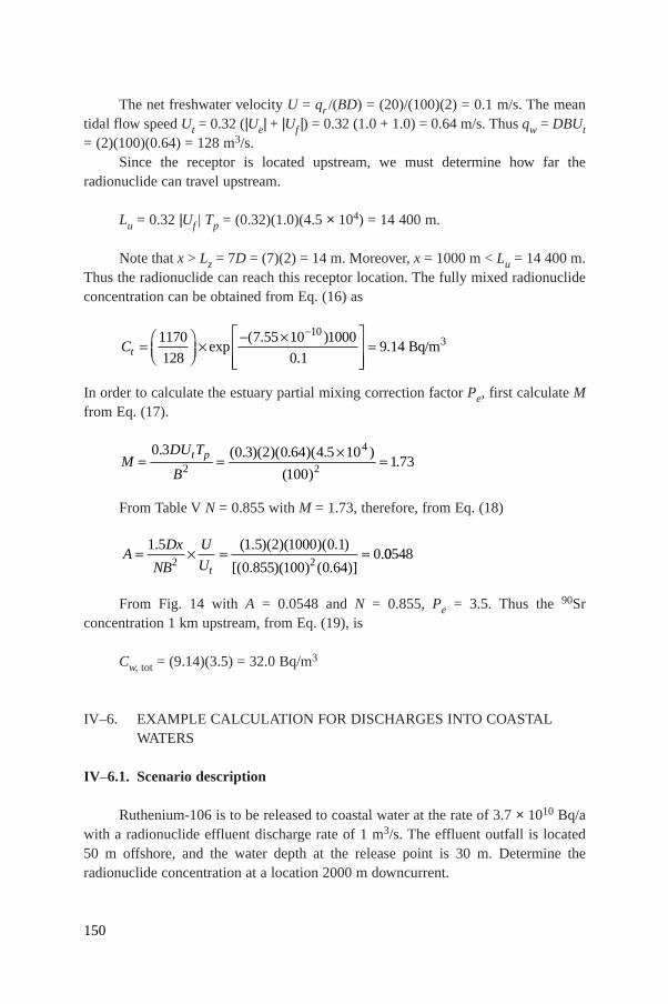
The net freshwater velocity U = qr /(BD) = (20)/(100)(2) = 0.1 m/s. The meantidal flow speed Ut = 0.32 (|Ue| + |Uf |) = 0.32 (1.0 + 1.0) = 0.64 m/s. Thus qw = DBUt= (2)(100)(0.64) = 128 m3/s.

Since the receptor is located upstream, we must determine how far theradionuclide can travel upstream.

Lu = 0.32 |Uf | Tp = (0.32)(1.0)(4.5 × 104) = 14 400 m.

Note that x > Lz = 7D = (7)(2) = 14 m. Moreover,x = 1000 m < Lu = 14 400 m.Thus the radionuclide can reach this receptor location. The fully mixed radionuclideconcentration can be obtained from Eq. (16) as

In order to calculate the estuary partial mixing correction factor Pe, first calculate Mfrom Eq. (17).

From Table V N = 0.855 with M = 1.73, therefore, from Eq. (18)

From Fig. 14 with A = 0.0548 and N = 0.855, Pe = 3.5. Thus the 90Srconcentration 1 km upstream, from Eq. (19), is

Cw, tot = (9.14)(3.5) = 32.0 Bq/m3

IV–6. EXAMPLE CALCULATION FOR DISCHARGES INTO COASTALWATERS

IV–6.1. Scenario description

Ruthenium-106 is to be released to coastal water at the rate of 3.7 × 1010 Bq/awith a radionuclide effluent discharge rate of 1 m3/s. The effluent outfall is located50 m offshore, and the water depth at the release point is 30 m. Determine theradionuclide concentration at a location 2000 m downcurrent.

ADx

NB

U

Ut= ¥ = =

1 5 1 5 2 1000 0 1

0 855 100 0 640

2 2

. ( . )( )( )( . )

[( . )( ) ( . )].00548

MDU T

B

t p= = ¥ =0 3 0 3 2 0 64 4 5 10

1001 732

4

2

. ( . )( )( . )( . )

( ).

Ct = ÊËÁ

ˆ¯

¥- ¥È

ÎÍÍ

˘

˚˙˙

=-1170

128

7 55 10 1000

0 19 14

10

exp( . )

.. Bq/m3

150

IV–6.2. Calculational procedure

Qi = 3.7 × 1010 Bq/a = 1170 Bq/s,F = 1 m3/s

D = 30 m ,y0 = 50 m,U = 0.1 m/s (default value),x = 2000 m

λi = 2.18 × 10–8 s–1 (see Annex II)

The radionuclide concentration C is ‘For fishing’ (i.e. for use as the basis forradionuclide activity concentrations in fish), using Eq. (20)

For this situation Cw, tot = 3.48 Bq/m3 ‘For the shoreline’ (i.e. for use as the basisfor activity concentrations in shoreline sediments for calculation of external doses),using Eq. (21)

For this situation Cw, tot = 2.98 Bq/m3.

IV–7. EXAMPLE CALCULATION FOR DISCHARGES INTO A SMALL LAKE

IV–7.1. Scenario description

Cobalt-60 is to be discharged directly into a lake having a river inflow andoutflow. The radionuclide release rate is 3.7 × 107 Bq/a with a radionuclide effluentdischarge of 0.1 m3/s. The lake is 400 m long, 100 m wide and 10 m deep. The 30year low annual riverflow rate is not known, but the representative river width undera normal (mean annual) river discharge is estimated to be 10 m. The nearestpotentially exposed individual is living along the lake. What is the radionuclideconcentration in the lake water?

Cw,

( . )

( . )

( )( . ) ( )

( )( )exp

( .tot = ¥

- ¥962 0 1 1170

30 2000

7 28 100 17

1 17

55 2 34 2

2 34

8

0 1 50

2000

2 18 10 2000

0

)( . ) ( )

( )

exp( . )( )

.

.

È

ÎÍÍ

˘

˚˙˙

¥- ¥ -

..1

È

ÎÍÍ

˘

˚˙˙

Cwy y

,

.

.

.

exp( .

tot=

-

=¥ ¥

¥

¥ -¥ ¥

0

962 0 1 1170

30 2000

2 18 10 2000

0 17

1 17

8 ))

..

0 13 48

È

ÎÍÍ

˘

˚˙˙

= Bq/m3

151

IV–7.2. Calculational procedure

Qi = 3.7 × 107 Bq/a = 1.17 Bq/s,d⋅ = 0

F = 0.1 m3/s, B = 10 m,B = 100 m,D = 10 m,Al = (400)(100) = 40 000 m2

λi = 4.17 × 10–9 s–1 (Annex II)

Firstly, the 30 year low annual flow rate of the river must be estimated. FromTable III the mean annual river flow rate ¯qr = 1 m3/s, for B = 10 m. Thus qr = 1/3 =0.33 m3/s. The lake surface area Al = 40 000 m2 = 0.04 km2, that is < 400 km2; thus thelake is classified as a small lake. The lake volume is V = (400)(100)(10) = 400 000 m3.Note that (qr /V + λi) = (0.33/400 000) + 4.17 × 10–9 = 8.29 × 10–7 > 10–8.

Since there is no radionuclide contribution to the lake from its watershed,d⋅ = 0.Thus Q′i = Qi = 1.17 Bq/s. With Eq. (24) the totally mixed radionuclide concentrationin the lake is

IV–8. EXAMPLE CALCULATION OF RADIONUCLIDE CONCENTRATIONSIN SEDIMENT

IV–8.1. Scenario description

A nuclear facility has been discharging 137Cs and 131I into a river for 30 years.The concentrations of 137Cs and 131I in unfiltered river water are each determined tobe 100 Bq/m3 at a location along the river bank. The suspended sedimentconcentration there is 0.1 kg/m3 (or 100 mg/L). What are the 137Cs and 131Iconcentrations in the river bottom sediment and in the river shore sediment?

IV–8.2. Calculational procedure

Ss = 0.1 kg/m3, Te = 3.15 × 107 s

For 137Cs,Kd = 1000 L/kg and λi = 7.33 × 10–10 s–1 (see Table VI and Annex II).For 131I, Kd = 10 L/kg and λi = 9.98 × 10–7 s–1 (see Table VI and Annex II).

Cw,( . )

[ . ( . )( )].tot

3Bq/cm=+ ¥

=-1 17

0 33 4 17 10 400 0003 53

9

152

IV–8.2.1. 137Cs

From Eq. (27) the 137Cs concentration in the river bottom sediment is

From Eq. (28) the 137Cs concentration in the river shore sediment is

IV–8.2.2. 131I

From Eq. (27) the 131I concentration in the river bottom sediment is

From Eq. (28) the 131I concentration in the river shore sediment is

IV–9. EXAMPLE CALCULATION OF FOOD CONCENTRATIONS FROMATMOSPHERIC DEPOSITION

IV–9.1. Scenario description

Iodine-131 is released to the atmosphere, resulting in a continuous depositionrate of 1 Bq·m–2·d–1 over agricultural land. What are the annual averageconcentrations of 131I in crops, forage, milk and meat?

Cs s,

( . )( . )( . )( . )( )( )( )

( . )( . )( ) ( . )( . )

( . )( . ) .

=+

× −× ×

= =

− × ×

−

−01 0 001 10 60 100

1 0 001 01 10

1

9 98 10 315 10

5 99 0 0318 019

9 98 10 3 15 10

7 7

7 7

e

Bq/kg

Cs b,

( . )( . )( . )( . )( )( )

( . )( . )( ) ( . )( . )

. ( . ) .

=+

× −× ×

= × = ×

− × ×

−

−

−01 0 001 10 100

1 0 001 01 10

1

9 98 10 315 10

01 0 0318 318 10

9 98 10 3 15 10

7 7

3

7 7

e

Bq/kg

Cs s,

( . )( . )( . )( . )( )( )( )

( . )( . )( ) ( . )( . )

( )( . )

=+

× −× ×

= =

− × ×

−

−01 0 001 1000 60 100

1 0 001 01 1000

1

7 33 10 315 10

545 0 989 539

7 33 10 3 15 10

10 7

10 7

e

Bq/kg

Cs b,

( .( . )( . )( )( )

( . )( . )( )=

+¥

- -0 1 0 001 1000 100

1 0 001 0 1 1000

1 7 33e ¥¥ ¥

-

-

¥ ¥

= =

10 3 15 10

10 7

10 7

7 33 10 3 15 10

9 09 0 989 8 9

)( . )

( . )( . )

( . )( . ) . 99 Bq/kg

153

IV–9.2. Calculational procedure

IV–9.2.1. Concentrations in food crops from direct deposition

The concentration of 131I on vegetation surfaces owing to direct depositionfrom the atmosphere is given by Eq. (30).

whered⋅ = 1.0 Bq·m–2·d–1, α = 0.3 m2/kg (for fresh weight of food crops, fromTable VII), lEv = λi + λw = 8.62 × 10–2 [d–1] + 5 × 10–2 [d–1] ≈ 1.4 × 10–1 [d–1], λi =8.62 × 10–2d–1 (Annex II),λw = 5 × 10–2d–1 (Table VII) and te = 60 d (from Table VIII).

IV–9.2.2. Concentrations in food crops from uptake from soil

The concentration of 131I in soil based on a unit deposition rate from theatmosphere is given by Eq. (32).

where d⋅ =1.0 Bq·m–2·d–1, λEs = λi + λs = 8.62 × 10–2 [d–1] + 1.4 × 10–3 [d–1] = 8.8 ×10–2 [d–1], λi = 8.62 × 10–2 d–1 (Annex II), λs = 1.4 × 10–3 (Table X),tb = 1.1 × 104 d(Table VIII), and ρ = 260 kg/m2 for cultivated soil other than peat (Table IX). Thus

Cs =◊ ◊ - - ¥ ¥ ¥- - - -1 1 8 8 10 1 1 102 1 2 1 4[ ][ exp( . [ ] . [ ])]Bq m d d d

260 [kg/m22

2

d

Bq m d

kg m d

] . [ ]

[ ]

. [ ].

¥ ¥

=◊ ◊

¥ ¥ ◊ ◊=

- -

- -

- - -

8 8 10

1

260 8 8 104

2 1

2 1

2 144 10 2¥ - Bq/kg dry weight of soil

Cd t

sE b

E

s

s

=- - [ exp( )]1 l

rl

Cv, (

[ ] . [ / [

1

21 0 3

food crops)

2 1 1Bq m d m kg][1 exp( 1.4 10 d

=

◊ ◊ ¥ - - ¥- - - --

- -

- -

- -

¥¥

=◊ ◊

¥

=

1

1 1

1 1

1

d])]

1.4 10 d

Bq kg d

d

2.

] [

[ ]

. [ ]

. [ ]

60

0 3

1 4 10 1

11 Bq/kg fresh weight in food crops from direct deposition

Cd t

vE e

E

v

v,

[ exp( )]1

1=

- -a l

l

154

The concentration of 131I in vegetation resulting from uptake from soil is givenby Eq. (31).

Cv, 2 = Fv × Cs

where Fv = 0.02 for food crops fresh weight (Table XI).Therefore the concentrationof 131I in food crops owing to uptake of 131I from soil is Cv, 2 (food crops)= 0.02[unitless] × 4.4 × 10–2 [Bq/kg] = 8.8 × 10–4 Bq/kg fresh weight.

IV–9.2.3. Total concentration in food crops

The concentration of 131I in food crops from both direct deposition and uptakefrom soil is given by Eq. (33).

Cv (food crops)= (Cv, 1 (food crops)+ Cv, 2 (food crops)) exp(–λi th)

where th = 14 d (from Table VIII). Cv (food crops)= (2.1 [Bq/kg] + 8.8 × 10–4 [Bq/kg])× exp(–8.62 × 10–2 [d–1] × 14 [d]) = 6.3 × 10–1 Bq/kg fresh weight.

IV–9.2.4. Pasture concentrations

For pasture forage the concentration is calculated on a dry weight basis, and thesoil is assumed to be uncultivated (not ploughed). The necessary parameters are (a) αand te from Eq. (30), (b) Fv from Eq. (31), (c) ρ from Eq. (32) and (d) th from Eq. (33).The parameter values specific to forage are α = 3 m2/kg (Table VII), te = 30 d(Table VIII), Fv = 0.1 (Table XI),ρ = 130 kg/m2 (Table IX) and th = 0 (Table VIII).Therefore the concentration on forage owing to direct deposition of 131I is (Eq. (30))

= 21 Bq/kg dry weight forage

The concentration in pasture soil is (Eq. (32))

= 8.7 × 10–2 Bq/kg dry weight of soil

The uptake from soil by pasture vegetation is (Eq. (31))

Cs =◊ ◊ - - ¥ ¥ ¥- - - -1 [Bq m d ][1 exp( 8.8 10 [d ] 1.1 10 [d])]

130 [kg/m

2 1 2 1 4

22 2 1] 8.8 0 [d ]¥ ¥ - -1

Cv, ([ ] [ / ] [ exp( . [ ]

1

2 1 2 1 11 3 1 1 4 10pasture)

Bq m d m kg d=

◊ ◊ ¥ ¥ - - ¥- - - - ¥¥¥ -

30

1 4 10 1

[ ])]

. [ ]

d

d

155

Cv, 2 (pasture)= 0.1 [unitless] × 8.7 × 10–2 [Bq/kg] = 8.7 × 10–3 Bq/kg

The total contamination in pasture from direct deposition and uptake from soilis (Eq. (33)) Cv (pasture)= (2.1 × 101 [Bq/kg] + 8.7 × 10–3 [Bq/kg]) × exp(–8.62 × 10–2

[d–1] × 0 [d]) = 21 Bq/kg dry weight forage.

IV–9.2.5. Concentrations in stored feed and average concentrations for feeds

If pasture is harvested and stored for th = 90 d (Table VIII), the concentrationon stored feed is (Eq. (33))

Cp (pasture)= (2.1 × 101 [Bq/kg] + 8.7 × 10–3 [Bq/kg]) × exp(–8.62 × 10–2 [d–1]× 90 [d])

= 9.0 × 10–3 Bq/kg dry weight forage

Assuming that both dairy and beef cattle are fed a diet of 70% fresh forage(Table XII), the average annual concentration of 131I in animal feed is (Eq. (35))

Ca = fp Cv (pasture)+ (1 – fp) Cp (pasture)= 0.7 × 21 [Bq/kg] + (1 – 0.7) 9.0

× 10–3 [Bq/kg] = 15 Bq/kg dry weight

IV–9.2.6. Concentration in milk

Assuming that the concentration of 131I in water is negligible, the concentrationin milk is (Eq. (36))

CM = Fm Ca QM exp(–λi tm)

where Fm = 0.01 d/L (Table XI),Ca = 15 Bq/kg,QM = 16 kg/d (Table XII) and tm =1 d (Table VIII).

CM = 0.01 [d/L] × 15 [Bq/kg] × 16 [kg/d]× exp(–8.62 × 10–2 [d–1] × 1 [d]) = 2.2 Bq/L

IV–9.2.7. Concentration in meat

Likewise, the concentration of 131I in meat is (Eq. (37))

CF = Ff Ca Qf exp(–λi tf)

156

where Ff = 0.05 d/kg (Table XI),Ca = 15 Bq/kg,Qf = 12 kg/d (Table XII) and tf = 20 d(Table VIII).

Cf = 0.05 [d/kg] × 15 [Bq/kg] × 12 [kg/d] × exp(–8.62 × 10–2 [d–1] × 20 [d])= 1.6 Bq/kg in meat

IV–9.2.8. Summary

Cfood crops= 0.63 Bq/kg,Cpasture= 21 Bq/kg

Cmilk = 2.2 Bq/L,Cmeat= 1.6 Bq/kg

IV–10. EXAMPLE CALCULATION OF FOOD CONCENTRATIONS FROMCONCENTRATIONS IN WATER

IV–10.1. Scenario description

The water of a small lake located near a village contains water with aconcentration (Cw) of 99Tc of 1 Bq/m3. The lake is used by the inhabitants of thevillage for fishing and for irrigating crops and pasture fields. These fields are irrigatedon one day per week for a four month period each year. The quantity of water used inone day is about 9 L/m2. The soil in the agricultural area is a peat soil. Animals alsodrink the lake water. Calculate the concentration of 99Tc in the major food itemsproduced in the area (fish, food crops, milk and meat). Which mechanism contributesmost to plant contamination?

IV–10.2. Calculational procedure

The concentration of 99Tc in fish is given by Eq. (38).

CF = Cw Bp/1000

where Cw = 1 Bq/m3, Bp = 50 L/kg (Table XIII). Thus CF = 1 [Bq/m3] × 50[L/kg]/1000 m3/L = 0.050 Bq/kg.

The radionuclide concentration in vegetation is assumed to be due to irrigationonly. The deposition rate due to irrigation is given by Eq. (34).

d⋅ = Cw × Iw

157

where Cw = 1 Bq/m3 and Iw is the average irrigation rate (m3·m–2·d–1).For deposition on plant surfaces, the average irrigation rate over the irrigation

period is required; for deposition on soil, the annual average irrigation rate is required.The amount used in one day is 9 L/m2 for 16 days over a 120 day period (once a weekfor four months). Thus the average irrigation rate over the irrigation period is

The annual average irrigation rate

Therefore the deposition rate on vegetation during the irrigation period is

and the annual average deposition rate on soil is

The concentration of 99Tc on vegetation surfaces owing to direct depositionfrom irrigation is given by Eq. (30).

where d◊= 1.3 × 10–3 Bq◊m–2◊d–1, a = 0.3 m2/kg fresh weight for food crops

(Table VII) and 3 m2/kg dry weight for forage (Table VII),li = 8.92 × 10–9 d–1

(Annex II) and lw = 0.05 d–1 (Table VII), so lEv = li + lw = 8.92 × 10–9 [d–1] + 5 ×10–2 [d–1] = 5 × 10–2 [d–1], te = 60 d for food crops (Table VIII) and 30 d for forage(Table VIII).

Cv,. [ ] . [ ] [ exp( [

1

3 21 3 10 0 3 1 5 10=

¥ ◊ ◊ ¥ ¥ - - ¥ ¥- - - - -Bq m d m /kg d ] 62 1 2 1 00[d

d ]

Bq/kg fresh weight food crops

1

-

- -

-

¥

= ¥

1

2

3

5 10

7 4 10

])]

[

. from direct deposition,

Bq m d m /kg2 1 2

Cv,. [ ] [

1

31 3 10 3=

¥ ◊ ◊ ¥- - - ]] [ exp( [ ])]

[

.

¥ - - ¥ ¥¥

=

- - -

- -1 5 10

5 10

0 061

2 1

2

d ] 30[d

d ]

Bq/kgdry

1

1

wweight pasture from direct deposition

Cd t

vE e

E

v

v,

[ exp( )]1

1=

- -a l

l

d = ¥ ¥ ◊ ◊ = ¥ ◊ ◊- - - - - -1 4 3 103 4 1[ ] ( . )[Bq/m m m d ] 4.3 10 Bq m d3 2 1 4 2

d = ¥ ¥ ◊ ◊ = ¥ ◊ ◊- - - - - -1 1 3 10 1 3 103 3 3 1[ ] ( . )[ ] .Bq/m m m d Bq m d3 2 1 2

Iw (ann)3 –2 –1 3 –2 –1m m d

d

365dm m d= ¥ ◊ ◊ ¥ = ¥ ◊ ◊- -1 3 10

1204 3 103 4. [ ] . [ ]

Iw = ◊ ◊ ¥ = ◊ ◊ = ¥ ◊ ◊- - - - -916

1201 3 1 3 102 1 3 3 2 1[ ] . [ ] . [–L m d

d

dL m d m m d–2 1 ]]

158

The concentration of 99Tc in vegetation resulting from uptake from soil is givenby Eqs (31) and (32).

where Fv = 5 for food crops (fresh weight) (Table XI) and 80 for pasture (dry weight)(Table XI), d⋅ = 4.3 × 10–4 Bq⋅m–2⋅d–1, ρ = 100 kg/m2 of dry weight peat soil(Table IX) for food crops and 50 kg/m2 dry weight peat soil (Table IX) for pasture, λi= 8.92 × 10–9 d–1 (Annex II), λs = 0 (Table X) and λEs = λi + λs = 8.92 × 10–9 d–1.

It is assumed that after irrigation 99Tc is found in soil in non-anionic forms.This assumption is conservative and therefore suitable for screening calculations.

tb = 30 a ≈ 1.1 × 104 d (Table VIII)

The concentration of 99Tc in vegetation is produced by both direct depositionfrom irrigation and uptake from irrigated soil (Eq. (33)). Owing to the longradioactive half-life of 99Tc, the radioactive decay during the delay between harvestand consumption is negligible.

Cv = (Cv, 1 + Cv, 2) exp(–λi th) ≈ Cv, 1 + Cv, 2

where Cv, 1 = 7.4 × 10–3 Bq/kg for food crops and 0.061 Bq/kg for pasture andCv, 2 = 0.24 Bq/kg for food crops and 7.6 Bq/kg for pasture. Therefore Cv = 7.4 × 10–3

[Bq/kg] + 0.24 [Bq/kg] ≈ 0.25 Bq/kg fresh weight for food crops and Cv= 0.061[Bq/kg] + 7.6 [Bq/kg] ≈ 7.7 Bq/kg dry weight for pasture.

The concentration of 99Tc in animal feed is given by Eq. (35). For the case of99Tc the decrease of the concentration in pasture during the storage time is negligible,owing to the very long half-life of 99Tc. Thus the concentration in stored feed (CP) ispractically identical to the concentration in pasture (Cv) expressed in dry weight.

Ca = fp Cv + (1 – fp) Cp ≈ Cv = 7.7 Bq/kg of dry animal feed

Cv, 2 = ¥¥ ◊ ◊

¥- - ¥- - - - -

54.3 10 [Bq m d ]

100 [kg/m ]

1 exp( 8.92 10 [d4 2 1

2

9 1]] 1.1 10 [d])

8.92 10 [d ]

0.24 Bq/kg fresh weight of foo

4

9 1

¥ ¥¥

=

- -

dd crops from uptake

C 804.3 10 [Bq m d ]

50[kg/m ], 2

4 2 1

2v = ¥¥ ◊ ◊

¥- - - 11 exp( 8.92 10 [d ] 1.1 10 [d])

8.92 10 [d ]

9 1 4

9 1

- - ¥ ¥ ¥¥

=

- -

- -

7 6. Bq/kg ddry weight of pasture from uptake

C F C Fd t

v v s vbE

s

Es

,

[ exp( )]2

1= ¥ =

- - lrl

159

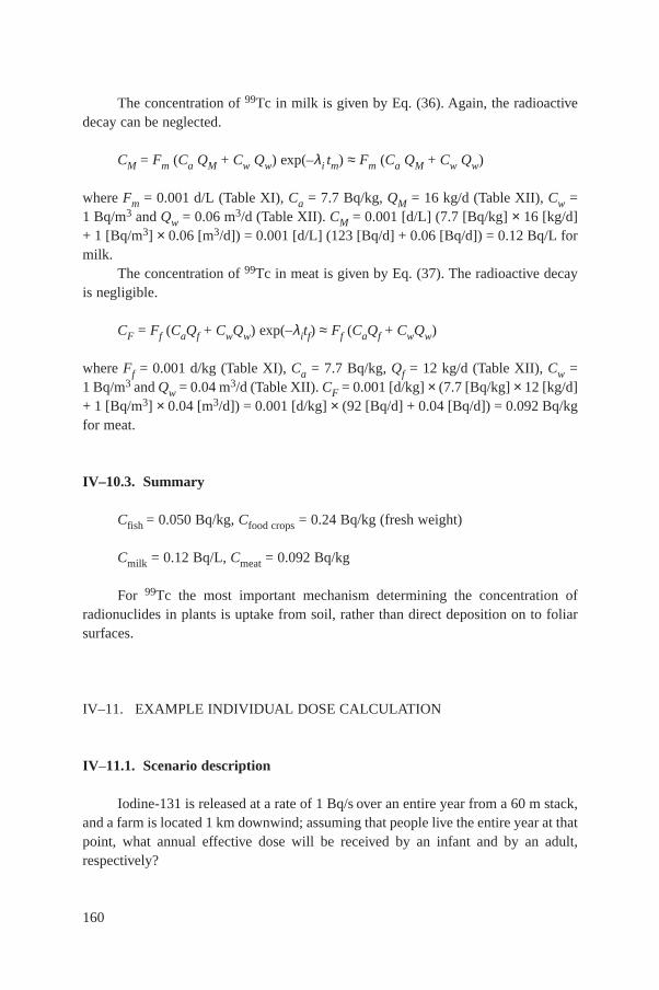
The concentration of 99Tc in milk is given by Eq. (36). Again, the radioactivedecay can be neglected.

CM = Fm (Ca QM + Cw Qw) exp(–λi tm) ≈ Fm (Ca QM + Cw Qw)

where Fm = 0.001 d/L (Table XI), Ca = 7.7 Bq/kg, QM = 16 kg/d (Table XII), Cw =1 Bq/m3 and Qw = 0.06 m3/d (Table XII). CM = 0.001 [d/L] (7.7 [Bq/kg] × 16 [kg/d]+ 1 [Bq/m3] × 0.06 [m3/d]) = 0.001 [d/L] (123 [Bq/d] + 0.06 [Bq/d]) = 0.12 Bq/L formilk.

The concentration of 99Tc in meat is given by Eq. (37). The radioactive decayis negligible.

CF = Ff (CaQf + CwQw) exp(–λitf) ≈ Ff (CaQf + CwQw)

where Ff = 0.001 d/kg (Table XI), Ca = 7.7 Bq/kg, Qf = 12 kg/d (Table XII), Cw =1 Bq/m3 and Qw = 0.04 m3/d (Table XII). CF = 0.001 [d/kg] × (7.7 [Bq/kg] × 12 [kg/d]+ 1 [Bq/m3] × 0.04 [m3/d]) = 0.001 [d/kg] × (92 [Bq/d] + 0.04 [Bq/d]) = 0.092 Bq/kgfor meat.

IV–10.3. Summary

Cfish = 0.050 Bq/kg, Cfood crops = 0.24 Bq/kg (fresh weight)

Cmilk = 0.12 Bq/L, Cmeat = 0.092 Bq/kg

For 99Tc the most important mechanism determining the concentration ofradionuclides in plants is uptake from soil, rather than direct deposition on to foliarsurfaces.

IV–11. EXAMPLE INDIVIDUAL DOSE CALCULATION

IV–11.1. Scenario description

Iodine-131 is released at a rate of 1 Bq/s over an entire year from a 60 m stack,and a farm is located 1 km downwind; assuming that people live the entire year at thatpoint, what annual effective dose will be received by an infant and by an adult,respectively?

160

IV–11.2. Calculational procedure

IV–11.2.1. Concentrations of radionuclides in air and on the ground

Assuming no building wake effects

assuming Pp = 0.25, ua = 2 m/s and F = 1 × 10–5 m–2 (from Table I), CA = 1.3 × 10–6

Bq/m3 and d⋅ = 1.3 × 10–6 × 1000 = 1.3 × 10–3 Bq⋅m–2⋅d–1

λEs = λi + λs = 0.0862 d–1 (Annex II) + 0.0014 d–1 (Table X) = 0.088 d–1, tB = 1.1 ×104 d (Table VIII). Therefore

IV–11.2.2. External dose from immersion in the plume

Eim = CA DFimOf

assuming DFim = 5.8 × 10–7 Sv/Bq (from Table XV) and Of = 1. Eim = 1.3 × 10–6 ×5.8 × 10–7 × 1 = 7.5 × 10–13 Sv/a.

IV–11.2.3. Dose from inhalation

The dose from inhalation is

Einh = CA Rinh DFinh

assuming Rinh = 1400 m3/a for infants and 8400 m3/a for adults (Table XIV) and Dinh= 7.2 × 10–8 Sv/Bq for infants and 7.4 × 10–9 Sv/Bq for adults (from Table XVI). Einh= 1.3 × 10–10 for infants and 8.1 × 10–11 Sv/a for adults.

Cgr =¥ - - ¥

=¥

-

-

( . ) exp[( . )( . )]

.

.

.

1 3 10 1 0 088 1 1 10

0 088

1 3 10

0 08

3 4

3

880 015 2= . Bq/m

Cd t

Es B

Esgr =

- -.[ exp( )]1 l

l

CP FQ

ud C VA

P i

aA T= =, ˙

161

IV–11.2.4. External dose from ground deposition

The external dose from ground deposition is

Egr = Cgr DFgrOf

assuming DFgr = 1.2 × 10–8 Sv/a per Bq/m2 (Table XV) and Of = 1. Egr = 0.015 × 1.2× 10–8 × 1 = 1.8 × 10–10 Sv/a.

IV–11.2.5. Dose from food ingestion

The dose from food ingestion is

Eing, p = Cp,i HpDing

Three food types are considered: crops, milk and meat. This calculation may beachieved by multiplying the example concentrations per unit deposition rate inSection 5 by the deposition rate of 1.3 × 10–3 Bq·m–2·d–1.

Ding = 1.8 × 10–7 for infants and 2.2 × 10–8 for adults (Table XVII)

(a) Crops: the concentration for unit deposition is 0.63 Bq/kg. Thus Cp,i = 0.63 ×1.3 × 10–3 = 8.2 × 10–4 Bq/kg, Hp = 150 for infants and 410 kg/a for adults(Table XIV). Thus Eing, crops = 8.2 × 10–4 × 150 × 1.8 × 10–7 = 2.2 × 10–8 Sv/afor infants and 8.2 × 10–4 × 410 × 2.2 × 10–8 = 7.4 × 10–9 Sv/a for adults.

(b) Milk: the concentration for unit deposition is 2.2 Bq/L. Thus Cp,i = 2.2 × 1.3 ×10–3 = 2.9 × 10–3 Bq/L, Hp = 300 for infants and 250 L/a for adults (Table XIV).Thus Eing, milk = 2.9 × 10–3 × 300 × 1.8 × 10–7 = 1.6 × 10–7 Sv/a for infants and2.9 × 10–3 × 250 × 2.2 × 10–8 = 1.6 × 10–8 Sv/a for adults.

(c) Meat: the concentration for unit deposition is 1.6 Bq/kg. Thus Cp,i = 1.6 × 1.3× 10–3 = 2.1 × 10–3 Bq/kg, Hp = 40 for infants and 100 kg/a for adults(Table XIV). Thus Eing, meat = 2.1 × 10–3 × 40 × 1.8 × 10–7 = 1.5 × 10–8 Sv/a forinfants and 2.1 × 10–3 × 100 × 2.2 × 10–8 = 4.6 × 10–9 Sv/a for adults.

Eing = 2.0 × 10–7 for infants and 2.8 × 10–8 for adults

IV–11.2.6. Total dose

The total individual dose is

E Ep ping ing= ∑ ,

162

Etot = Eim + Einh + Egr + Eing

Etot = 7.5 × 10–13 + 1.3 × 10–10 + 1.8 × 10–10 + 2.0 × 10–7 = 2.0 × 10–7 Sv/a for infants

and

Etot = 7.5 × 10–13 + 8.1 × 10–11 + 1.8 × 10–10 + 2.8 × 10–8 = 2.8 × 10–8 Sv/a for adults

IV–12. EXAMPLE COLLECTIVE DOSE CALCULATION

IV–12.1. Scenario description

A facility intends to discharge 4 × 103 Bq/a of 131I to the atmosphere and 6 × 104

Bq/a into the sea. What are the approximate collective doses due to these discharges?

IV–12.2. Calculational procedure

For discharges to the atmosphere, the screening collective effective dosecommitment per unit activity of 131I discharged is 10–12 man·Sv/Bq (Table XIX).

The collective effective dose commitment for each year of discharge istherefore

10–12 × (4 × 103) = 4 × 10–9 man·Sv

If the discharge continued for 30 years, the total collective dose commitmentwould be

30 × (4 × 10–9) = 1.2 × 10–7 man·Sv

Similarly, for discharges into the sea, the screening collective dose commitmentper unit activity of liquid 131I discharged is 10–16 man·Sv/Bq (Table XX). Thecollective effective dose commitment for each year of discharge is therefore

10–16 × (6 × 104) = 6 × 10–12 man·Sv

If the discharge continued for 30 years, the total collective dose commitmentwould be

30 × (6 × 10–11) = 1.8 × 10–10 man·Sv

163

164

Annex V

DESCRIPTION OF THE GAUSSIAN PLUME MODEL

For a continuous release from an elevated point source under constant windvelocity and atmospheric conditions the Gaussian plume model [V–1, V–2] may berepresented by

(V–1)

where

CA(x,y,z) is the air concentration (Bq/m3) at a point (x,y,z) downwind of the release;x is the downwind distance (m);y is the crosswind distance (m);z is the height above ground (m);Qi is the release rate for radionuclide i (Bq/s);σy,σz are the diffusion parameters (m), which are a function of downwind

distance x and atmospheric stability;u is the mean wind speed (m/s);H is the height of release (m).

The value of H used in the Gaussian plume model is the physical stack heightof the release point plus an allowance for any additional plume rise owing tomomentum, for example fan driven exhausts, or buoyancy for significantly heatedexhausts. In most cases involving the release of radionuclides the effective stackheight corresponds closely to the physical stack height.

The diffusion parameters used in the Gaussian plume model incorporate thebasic assumption of the model that a plume spreads both laterally and vertically witha Gaussian distribution. The form of the model represented by Eq. (V–1) includesreflection of the plume at ground level.

In theory, the Gaussian plume model is limited to rather simple dispersionsituations [V–3].

(a) Dispersion over flat, non-complex terrain;(b) Short range transport (about 100 m to 20 km downwind);(c) Steady state meteorological conditions;(d) No elevated temperature inversions;(e) Quasi-continuous releases;

C x,y,zy z H

A ( ) exp= -Ê

ËÁÁ

ˆ

¯˜ -

( )È

ÎÍÍ

˘

˚

Q

u

–i

y z2 2 2

2 2

2 2ps s s sy z

exp ˙˙

-( )È

ÎÍÍ

˘

˚˙˙

ÏÌÔ

ÓÔ

¸˝Ô

Ô+

+exp

z H2

2 2s z

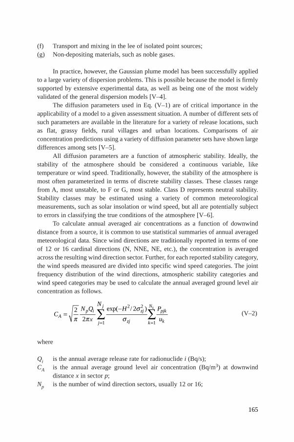
(f) Transport and mixing in the lee of isolated point sources;(g) Non-depositing materials, such as noble gases.

In practice, however, the Gaussian plume model has been successfully appliedto a large variety of dispersion problems. This is possible because the model is firmlysupported by extensive experimental data, as well as being one of the most widelyvalidated of the general dispersion models [V–4].

The diffusion parameters used in Eq. (V–1) are of critical importance in theapplicability of a model to a given assessment situation. A number of different sets ofsuch parameters are available in the literature for a variety of release locations, suchas flat, grassy fields, rural villages and urban locations. Comparisons of airconcentration predictions using a variety of diffusion parameter sets have shown largedifferences among sets [V–5].

All diffusion parameters are a function of atmospheric stability. Ideally, thestability of the atmosphere should be considered a continuous variable, liketemperature or wind speed. Traditionally, however, the stability of the atmosphere ismost often parameterized in terms of discrete stability classes. These classes rangefrom A, most unstable, to F or G, most stable. Class D represents neutral stability.Stability classes may be estimated using a variety of common meteorologicalmeasurements, such as solar insolation or wind speed, but all are potentially subjectto errors in classifying the true conditions of the atmosphere [V–6].

To calculate annual averaged air concentrations as a function of downwinddistance from a source, it is common to use statistical summaries of annual averagedmeteorological data. Since wind directions are traditionally reported in terms of oneof 12 or 16 cardinal directions (N, NNE, NE, etc.), the concentration is averagedacross the resulting wind direction sector. Further, for each reported stability category,the wind speeds measured are divided into specific wind speed categories. The jointfrequency distribution of the wind directions, atmospheric stability categories andwind speed categories may be used to calculate the annual averaged ground level airconcentration as follows.

(V–2)

where

Qi is the annual average release rate for radionuclide i (Bq/s);CA is the annual average ground level air concentration (Bq/m3) at downwind

distance x in sector p;Np is the number of wind direction sectors, usually 12 or 16;

CQ H P

uAi zj

zjj

pjk

kk

=-

= =Â Â2

2

22 2

1 1p p

ss

NN

pj Nk

x

exp( / )

165

Ppjk is the joint frequency of wind direction sector p, stability category j and windspeed class k;

Nk is the number of wind speed classes;Nj is the number of stability categories;uk is the wind speed associated with wind speed class k (m/s);σzj is the vertical diffusion parameter (m) associated with stability category j.

Equation (V–2) is often used in environmental radiological dose assessmentcalculations. However, proper use of this form of the Gaussian plume model requiresappropriate long term meteorological information for the site of interest. In addition,a computer may be necessary for managing all of the individual terms that must besummed in order to obtain the final average air concentration estimate. Equation(V–2) forms the basis for most of the screening procedures presented in Section 3.

REFERENCES

[V–1] GIFFORD, F.A., “An outline of theories of diffusion in the lower layers of theatmosphere”, Meteorology and Atomic Energy (SLADE, D.H., Ed.), Rep. TID-24 190,United States Army Environmental Center, Washington, DC (1968).

[V–2] PASQUILL, F., SMITH, F.B., Atmospheric Diffusion, 3rd edn, Ellis Horwood,Chichester (1983).

[V–3] TILL, J.E., MEYER, H.R. (Eds), Radiological Assessment — A Textbook onEnvironmental Dose Analysis, Rep. NUREG/CR-3332, ORNL-5968, United StatesNuclear Regulatory Commission, Washington, DC (1983).

[V–4] NATIONAL COUNCIL ON RADIATION PROTECTION AND MEASUREMENTS,Radiological Assessment: Predicting the Transport, Bioaccumulation, and Uptake byMan of Radionuclides Released to the Environment, Rep. No. 76, NCRP, Bethesda, MD(1984).

[V–5] VOGT, K.J., Empirical investigations of the diffusion of waste air plumes in theatmosphere, Nucl. Technol. 34 (1977) 43–57.

[V–6] INTERNATIONAL ATOMIC ENERGY AGENCY, Generic Models and Parameters forAssessing the Environmental Transfer of Radionuclides from Routine Releases:Exposures of Critical Groups, Safety Series No. 57, IAEA, Vienna (1982).

166

167

Annex VI

RADIONUCLIDE TRANSPORT IN SURFACE WATERS

The mathematical expressions discussed in Section 4 for rivers, estuaries,coastal waters, small lakes and large lakes are derived in this annex, and theassociated assumptions are outlined. In general, radionuclide transport and fate insurface waters may be expressed in the following three dimensionaladvection–diffusion equation [VI–1, VI–2].

(VI–1)

where

Cw, tot is the radionuclide concentration (Bq/m3);U, V, W are the flow velocities in the x, y and z directions, respectively (m/s);S is the radionuclide addition or subtraction, for example production of a

daughter product (Bq·m–3·s–1);t is the time (s);x, y, z are the longitudinal, lateral and vertical directions, respectively, in

Cartesian co-ordinates (m); ex, ey, ez are the dispersion coefficients in the x, y and z directions, respectively

(m2/s);li is the radionuclide decay constant (s–1).

Various simplifications were applied to this general governing equation toobtain the appropriate solutions used in this Safety Report. The radionuclide transportmodels described here are for use in estimating radionuclide concentrations forsteady, continuous releases of radionuclides into each of the five types of surfacewater with steady state flow conditions. For time varying radionuclide release casesradionuclide concentrations in a receiving surface water body may be obtained byusing the convolution technique [VI–3].

∂∂

+∂

∂+

∂∂

+∂

∂

=∂

∂+

C

tU

C

xV

C

yW

C

z

C

x

w w w w

xw

, , , ,

,

tot tot tot tot

tote e2

2 yyw

zw

i w

C

y

C

zC S

∂

∂+

∂

∂- +

2

2

2

2

, ,,

tot tottote l

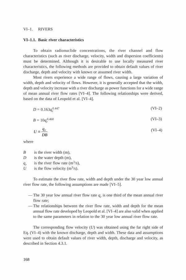
VI–1. RIVERS

VI–1.1. Basic river characteristics

To obtain radionuclide concentrations, the river channel and flowcharacteristics (such as river discharge, velocity, width and dispersion coefficients)must be determined. Although it is desirable to use locally measured rivercharacteristics, the following methods are provided to obtain default values of riverdischarge, depth and velocity with known or assumed river width.

Most rivers experience a wide range of flows, causing a large variation ofwidth, depth and velocity of flows. However, it is generally accepted that the width,depth and velocity increase with a river discharge as power functions for a wide rangeof mean annual river flow rates [VI–4]. The following relationships were derived,based on the data of Leopold et al. [VI–4].

D = 0.163qr0.447 (VI–2)

B = 10qr0.460 (VI–3)

(VI–4)

where

B is the river width (m),D is the water depth (m),qr is the river flow rate (m3/s),U is the flow velocity (m3/s).

To estimate the river flow rate, width and depth under the 30 year low annualriver flow rate, the following assumptions are made [VI–5].

— The 30 year low annual river flow rate qr is one third of the mean annual riverflow rate;

— The relationships between the river flow rate, width and depth for the meanannual flow rate developed by Leopold et al. [VI–4] are also valid when appliedto the same parameters in relation to the 30 year low annual river flow rate.

The corresponding flow velocity (U) was obtained using the far right side ofEq. (VI–4) with the known discharge, depth and width. These data and assumptionswere used to obtain default values of river width, depth, discharge and velocity, asdescribed in Section 4.3.1.

Uq

DBr=

168

VI–1.2. Dispersion coefficients and complete mixing distances

Dispersion coefficients vary significantly from river to river, or with riverchannel and flow conditions even in the same river [VI–6]. Examples of longitudinaland lateral dispersion coefficients for different rivers are shown in Tables VI–I andVI–II [VI–3, VI–6, VI–7].

The most common expression of vertical dispersion coefficient in a river is[VI–3]

ez = 0.067u*D (VI–5)

where

ez is the vertical dispersion coefficient (m2/s),u

*is the shear velocity (m/s).

Longitudinal and lateral dispersion coefficients in rivers vary by several ordersof magnitude from small creeks to large rivers such as the Mississippi and ColumbiaRivers, and there are many formulations available to estimate these coefficients[VI–3, VI–5, VI–6]. The following expressions provide reasonably good estimates ofthe longitudinal and lateral dispersion coefficients over a wide range of riverconditions [VI–3, VI–6].

(VI–6)

ey = aDu*

(VI–7)

where

ex, ey are the longitudinal and lateral dispersion coefficients, respectively (m2/s);a is the proportionality coefficient.

The proportionality coefficient a between ey and Du*

in Eq. (VI–7) varies witha width to depth ratio ranging from 0.1 to 0.2 for small laboratory flumes and mediumsized irrigation canals to 0.6 to 2.0 for the Missouri and MacKenzie Rivers [VI–3,VI–7]. In this report we have selected a = 0.6. Assuming that [VI–7]

u*

= 0.1U (VI–8)

and substituting Eq. (VI–8) into Eq. (VI–5) yields

exU B

Du=

2 2

30*

169

170

TABLE VI–I. EXAMPLES OF LONGITUDINAL DISPERSION COEFFICIENTSIN RIVERS

Mean Mean Shear Dispersion

ChannelWidth, depth, velocity, velocity, coefficient,

B D U u*

ex ex/Du*

(m) (m) (m/s) (m/s) (m2/s)

Chicago Ship Canal 48.8 8.07 0.27 0.0191 3.0 20

Sacramento River 4.00 0.53 0.051 15 74

River Derwent 0.25 0.38 0.14 4.6 131

South Platte River 0.46 0.66 0.069 16.2 510

Yuma Mesa A Canal 3.45 0.68 0.345 0.76 8.6

Green–Duwamish

River 20 1.10 0.049 6.5–8.5 120–160

Missouri River 200 2.70 1.55 0.074 1500 7500

Copper Creek 16 0.49 0.27 0.080 20 500

18 0.85 0.60 0.100 21 250

16 0.49 0.26 0.080 9.5 245

19 0.40 0.16 0.116 9.9 220

Clinch River, 47 0.85 0.32 0.067 14 235

Tennessee 60 2.10 0.94 0.104 54 245

53 2.10 0.83 0.107 47 210

Clinch River,

Virginia 36 0.58 0.21 0.049 8.1 280

Powell River 34 0.85 0.15 0.055 9.5 200

Coachella Canal 24 1.56 0.71 0.043 9.6 140

Bayou Anacoco 26 0.94 0.34 0.067 33 520

37 0.91 0.40 0.067 39 640

Nooksack River 64 0.76 0.67 0.27 35 170

Wind/Bighorn 59 1.10 0.88 0.12 42 320

Rivers 69 2.16 1.55 0.17 160 440

John Day River 25 0.58 1.01 0.14 14 170

34 2.47 0.82 0.18 65 150

Comite River 16 0.43 0.37 0.05 14 650

Sabine River 104 2.04 0.58 0.05 315 3100

127 4.75 0.64 0.08 670 1800

Yadkin River 70 2.35 0.43 0.10 110 470

72 3.84 0.76 0.13 260 520

171

TABLE VI–II. EXAMPLES OF LATERAL DISPERSION COEFFICIENTS IN RIVERS

Channel, Mean Mean Shear Lateral

River Channel descriptionwidth, depth, velocity, velocity, dispersion

B D U u*

coefficient, ey ey/Du*

(m) (m) (m/s) (m/s) (m2/s)

Missouri River near Blair, Nebraska Meandering river 200 2.7 1.75 0.074 0.12 0.6Ijssel River Groins on sides and gentle

curvature 69.5 4.0 0.96 0.075 0.15 0.51Mackenzie River from Fort Simpson Generally straight alignment

to Norman Wells or slight curvature; numerousislands and sand bars 1240 6.7 1.77 0.152 0.67 0.66

Missouri River downstream of Reach includes one 90° andCooper Nuclear Station, Nebraska one 180° bend 210–270 4.0 5.4 0.08 1.1 3.4

Potomac River; 29 km reach below Gently meandering riverthe Dickerson Power Plant with up to 60° bends 350 0.73–1.74 0.29–0.58 0.033–0.051 0.013–0.058 0.52–0.65

Aristo Feeder Canal 18.3 0.67 0.67 0.062 0.0093 0.22Bernado Conveyance Channel 20.1 0.70 1.25 0.061 0.013 0.30Athabasca River Below Fort McMurray 373 2.19 0.95 0.056 0.092 0.75Athabasca River Below Athabasca 320 2.05 0.86 0.079 0.066 0.41North Saskatchewan River Below Edmonton 213 1.55 0.58 0.080 0.031 0.25Bow River At Calgary 104 1.00 1.05 0.139 0.085 0.61Beaver River Near Cold Lake 42.7 0.96 0.50 0.044 0.042 0.99Grand River Below Kitchener 59.2 0.51 0.35 0.069 0.0090 0.26Columbia River 305 3.05 1.35 0.088 0.20 0.75Missouri River Two mild alternating bends 183 2.66 1.74 0.073 0.12 0.62Missouri River Sinuous, severe bends 234 3.96 1.98 0.042 0.55 3.3South River Few mild bends 18.2 0.40 0.21 0.040 0.0048 0.30Lesser Slave River Contorted meander 43.0 2.53 0.65 0.049 0.041 0.33Mobile River Mostly straight, one mild curve 430 4.93 0.30 0.018 0.64 7.2

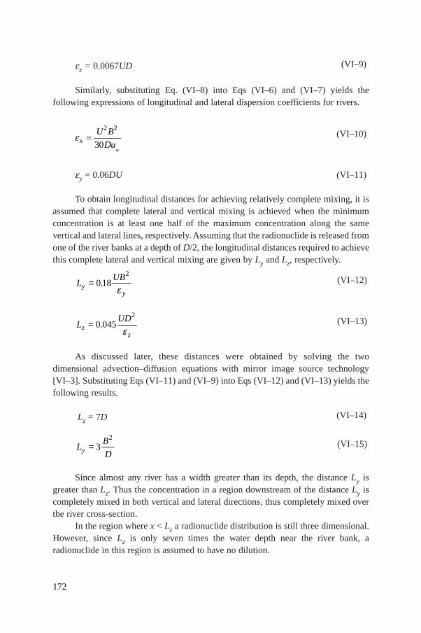
ez = 0.0067UD (VI–9)

Similarly, substituting Eq. (VI–8) into Eqs (VI–6) and (VI–7) yields thefollowing expressions of longitudinal and lateral dispersion coefficients for rivers.

(VI–10)

ey = 0.06DU (VI–11)

To obtain longitudinal distances for achieving relatively complete mixing, it isassumed that complete lateral and vertical mixing is achieved when the minimumconcentration is at least one half of the maximum concentration along the samevertical and lateral lines, respectively. Assuming that the radionuclide is released fromone of the river banks at a depth of D/2, the longitudinal distances required to achievethis complete lateral and vertical mixing are given by Ly and Lz, respectively.

(VI–12)

(VI–13)

As discussed later, these distances were obtained by solving the twodimensional advection–diffusion equations with mirror image source technology[VI–3]. Substituting Eqs (VI–11) and (VI–9) into Eqs (VI–12) and (VI–13) yields thefollowing results.

Lz = 7D (VI–14)

(VI–15)

Since almost any river has a width greater than its depth, the distance Ly isgreater than Lz. Thus the concentration in a region downstream of the distance Ly iscompletely mixed in both vertical and lateral directions, thus completely mixed overthe river cross-section.

In the region where x < Lz a radionuclide distribution is still three dimensional.However, since Lz is only seven times the water depth near the river bank, aradionuclide in this region is assumed to have no dilution.

LB

Dy = 32

LUD

zz

= 0 0452

.ε

LUB

yy

= 0 182

.ε

172

exU B

Du=

2 2

30*

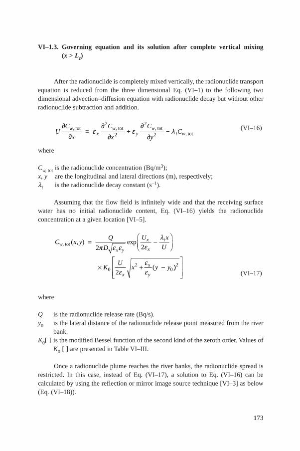
VI–1.3. Governing equation and its solution after complete vertical mixing(x > Lz)

After the radionuclide is completely mixed vertically, the radionuclide transportequation is reduced from the three dimensional Eq. (VI–1) to the following twodimensional advection–diffusion equation with radionuclide decay but without otherradionuclide subtraction and addition.

(VI–16)

where

Cw, tot is the radionuclide concentration (Bq/m3);x, y are the longitudinal and lateral directions (m), respectively;li is the radionuclide decay constant (s–1).

Assuming that the flow field is infinitely wide and that the receiving surfacewater has no initial radionuclide content, Eq. (VI–16) yields the radionuclideconcentration at a given location [VI–5].

(VI–17)

where

Q is the radionuclide release rate (Bq/s).y0 is the lateral distance of the radionuclide release point measured from the river

bank.K0[ ] is the modified Bessel function of the second kind of the zeroth order. Values of

K0 [ ] are presented in Table VI–III.

Once a radionuclide plume reaches the river banks, the radionuclide spread isrestricted. In this case, instead of Eq. (VI–17), a solution to Eq. (VI–16) can becalculated by using the reflection or mirror image source technique [VI–3] as below(Eq. (VI–18)).

C x yQ

D

U x

U

KU

x y y

wx y

x

x

i

x

x

y

, ( , ) exp

(

tot = -ÊËÁ

ˆ¯

¥ + -

2 2

202

0

p e e el

eee

))2È

ÎÍÍ

˘

˚˙˙

UC

x

C

x

C

yC

wx

wy

wi w

∂∂

=∂

∂+

∂

∂−, , ,

,tot tot tot

totε ε λ2

2

2

2

173

174

0.0 •0.1 2.68 232 610 23

0.2 2.14 075 732 33

0.3 1.85 262 730 07

0.4 1.66 268 208 91

0.5 1.52 410 938 57

0.6 1.41 673 762 14

0.7 1.33 012 365 62

0.8 1.25 820 312 16

0.9 1.19 716 338 03

1.0 1.14 446 307 97

1.1 1.09 833 028 28

1.2 1.05 748 453 22

1.3 1.02 097 316 13

1.4 0.98 806 999 61

1.5 0.95 821 005 33

1.6 0.93 094 598 08

1.7 0.90 591 813 86

1.8 0.88 283 352 70

1.9 0.86 145 061 68

2.0 0.84 156 821 51

2.1 0.82 301 715 25

2.2 0.80 565 398 12

2.3 0.78 935 613 12

2.4 0.77 401 814 07

2.5 0.75 954 869 03

2.6 0.74 586 824 30

2.7 0.73 290 715 15

2.8 0.72 060 412 51

2.9 0.70 890 497 74

3.0 0.69 776 159 80

3.1 0.68 713 110 10

3.2 0.67 697 511 39

3.3 0.66 725 918 31

3.4 0.65 795 227 25

3.5 0.64 902 633 77

3.6 0.64 045 596 47

3.7 0.63 221 805 91

3.8 0.62 429 158 12

3.9 0.61 665 731 47

4.0 0.60 929 766 93

4.1 0.60 219 650 64

4.2 0.59 533 898 89

4.3 0.58 871 144 86

4.4 0.58 230 127 04

4.5 0.57 609 678 97

4.6 0.57 008 720 22

4.7 0.56 426 248 40

4.8 0.55 861 331 94

4.9 0.55 313 103 97

5.0 0.54 780 756 43

5.1 0.54 263 535 19

5.2 0.53 760 735 40

5.3 0.53 271 697 44

5.4 0.52 795 803 29

5.5 0.52 332 473 16

5.6 0.51 881 162 52

5.7 0.51 441 359 38

5.8 0.51 012 581 83

5.9 0.50 594 375 83

6.0 0.50 186 313 09

6.1 0.49 787 989 29

6.2 0.49 399 022 37

6.3 0.49 019 050 93

6.4 0.48 647 732 91

6.5 0.48 284 744 13

6.6 0.47 929 777 29

6.7 0.47 582 540 66

6.8 0.47 242 757 23

6.9 0.46 910 163 70

7.0 0.46 584 509 59

7.1 0.46 265 556 57

7.2 0.45 953 077 56

7.3 0.45 646 856 18

7.4 0.45 346 685 94

7.5 0.45 052 369 91

7.6 0.44 763 719 96

7.7 0.44 480 556 36

7.8 0.44 202 707 24

7.9 0.43 930 008 19

8.0 0.43 662 301 85

8.1 0.43 399 437 54

8.2 0.43 141 270 84

8.3 0.42 887 663 29

8.4 0.42 638 482 14

8.5 0.42 393 599 93

8.6 0.42 152 894 33

8.7 0.41 916 247 81

8.8 0.41 683 547 43

8.9 0.41 454 684 62

9.0 0.41 229 554 93

9.1 0.41 008 057 83

9.2 0.40 790 096 62

9.3 0.40 364 412 45

9.5 0.40 156 513 22

9.6 0.39 951 796 93

9.7 0.39 750 183 13

9.8 0.39 551 594 16

9.9 0.39 355 955 06

10.0 0.39 163 193 44

10.2 0.38 786 025 39

10.4 0.38 419 558 46

10.6 0.38 063 295 49

10.8 0.37 716 771 25

11.0 0.37 379 549 71

11.2 0.37 051 221 56

11.4 0.36 731 402 43

11.6 0.36 419 730 76

TABLE VI–III. MODIFIED BESSEL FUNCTIONS OF THE SECOND KIND OFTHE ZEROTH ORDER

Modified Bessel functions Modified Bessel functions Modified Bessel functionsx exK0(x) x exK0(x) x exK0(x)

175

11.8 0.36 115 866 16

12.0 0.35 819 487 84

12.2 0.35 530 293 18

12.4 0.35 247 996 43

12.6 0.34 972 327 46

12.8 0.34 703 030 81

13.0 0.34 439 864 55

13.2 0.34 182 599 43

13.4 0.33 931 018 06

13.6 0.33 684 914 05

13.8 0.33 444 091 42

14.0 0.33 208 363 83

14.2 0.32 977 554 02

14.4 0.32 751 493 32

14.6 0.32 530 020 91

14.8 0.32 312 983 64

15.0 0.32 100 235 34

15.2 0.31 891 636 55

15.4 0.31 687 054 05

15.6 0.31 486 360 51

15.8 0.31 289 434 24

16.0 0.31 096 158 80

16.2 0.30 906 422 69

16.4 0.30 720 119 19

16.6 0.30 537 145 92

16.8 0.30 357 404 87

17.0 0.30 180 801 93

17.2 0.30 007 246 78

17.4 0.29 836 652 76

17.6 0.29 668 936 57

17.8 0.29 504 018 17

18.0 0.29 341 820 62

18.2 0.29 182 269 87

18.4 0.29 025 294 72

18.6 0.28 870 826 54

18.8 0.28 718 799 33

19.0 0.28 569 149 44

19.2 0.28 421 815 54

19.4 0.28 276 738 48

19.6 0.28 133 861 17

19.8 0.27 993 128 62

20.0 0.27 854 487 66

TABLE VI–III. (cont.)

Modified Bessel functions Modified Bessel functions Modified Bessel functionsx exK0(x) x exK0(x) x exK0(x)

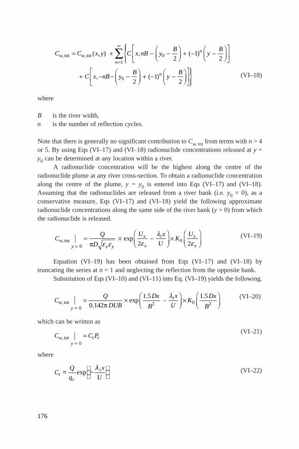
(VI–18)

where

B is the river width,n is the number of reflection cycles.

Note that there is generally no significant contribution to Cw, tot from terms with n > 4or 5. By using Eqs (VI–17) and (VI–18) radionuclide concentrations released at y =y0 can be determined at any location within a river.

A radionuclide concentration will be the highest along the centre of theradionuclide plume at any river cross-section. To obtain a radionuclide concentrationalong the centre of the plume, y = y0 is entered into Eqs (VI–17) and (VI–18).Assuming that the radionuclides are released from a river bank (i.e. y0 = 0), as aconservative measure, Eqs (VI–17) and (VI–18) yield the following approximateradionuclide concentrations along the same side of the river bank (y = 0) from whichthe radionuclide is released.

(VI–19)

Equation (VI–19) has been obtained from Eqs (VI–17) and (VI–18) bytruncating the series at n = 1 and neglecting the reflection from the opposite bank.

Substitution of Eqs (VI–10) and (VI–11) into Eq. (VI–19) yields the following.

(VI–20)

which can be written as

(VI–21)

where

(VI–22)CQ

q

x

Utr

i= −

expλ

C C Pwy

t r, tot=

=0

CQ

DUB

Dx

B

x

UK

Dx

Bw

y

i, .

exp. .

tot=

= ¥ -ÊËÁ

ˆ¯

¥ ÊËÁ

ˆ¯0

2 0 20 142

1 5 1 5

pl

CQ

D

U x

UK

Uw

y x y

x

x

i x

x, exptot

== ¥ -

ÊËÁ

ˆ¯

¥ÊËÁ

ˆ¯0

02 2p e e el

e

C C x y C x nB yB

yB

w wn

, , ( , ) , ( )tot tot= + - -ÊËÁ

ˆ¯

+ - -ÊËÁ

ˆ¯

È

ÎÍ

˘

˚˙0 2

12

ÏÏÌÔ

ÓÔ

+ - - -ÊËÁ

ˆ¯

+ - -ÊËÁ

ˆ¯

È

ÎÍ

˘

˚˙¸˝ÔÔ

=

•

Ân

nC x nB yB

yB

1

0 21

2, ( )

176

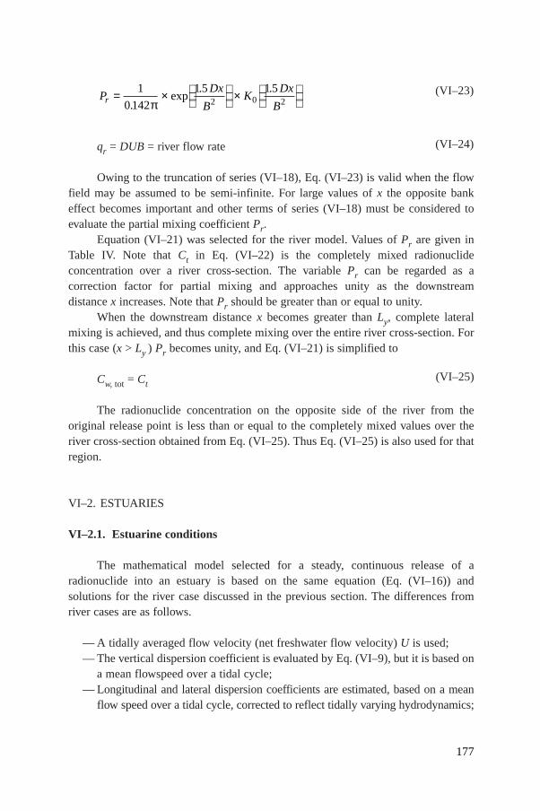
(VI–23)

qr = DUB = river flow rate (VI–24)

Owing to the truncation of series (VI–18), Eq. (VI–23) is valid when the flowfield may be assumed to be semi-infinite. For large values of x the opposite bankeffect becomes important and other terms of series (VI–18) must be considered toevaluate the partial mixing coefficient Pr.

Equation (VI–21) was selected for the river model. Values of Pr are given inTable IV. Note that Ct in Eq. (VI–22) is the completely mixed radionuclideconcentration over a river cross-section. The variable Pr can be regarded as acorrection factor for partial mixing and approaches unity as the downstreamdistance x increases. Note that Pr should be greater than or equal to unity.

When the downstream distance x becomes greater than Ly, complete lateralmixing is achieved, and thus complete mixing over the entire river cross-section. Forthis case (x > Ly ) Pr becomes unity, and Eq. (VI–21) is simplified to

Cw, tot = Ct(VI–25)

The radionuclide concentration on the opposite side of the river from theoriginal release point is less than or equal to the completely mixed values over theriver cross-section obtained from Eq. (VI–25). Thus Eq. (VI–25) is also used for thatregion.

VI–2. ESTUARIES

VI–2.1. Estuarine conditions

The mathematical model selected for a steady, continuous release of aradionuclide into an estuary is based on the same equation (Eq. (VI–16)) andsolutions for the river case discussed in the previous section. The differences fromriver cases are as follows.

— A tidally averaged flow velocity (net freshwater flow velocity) U is used;— The vertical dispersion coefficient is evaluated by Eq. (VI–9), but it is based on

a mean flowspeed over a tidal cycle;— Longitudinal and lateral dispersion coefficients are estimated, based on a mean

flow speed over a tidal cycle, corrected to reflect tidally varying hydrodynamics;

PDx

BK

Dx

Br = ×

×

1

0 142

1 5 1 52 0 2.

exp. .

π

177

178

— Water use locations both upstream and downstream from the radionucliderelease point are analysed, and the radionuclide concentration in the upstreamlocation can be corrected for the tidal effect [VI–7, VI–8].

VI–2.2. Dispersion coefficients and complete mixing distances

Dispersion processes occurring in estuaries are very complex, generally morecomplex than those occurring in rivers, owing to the additional effects of tides,density stratification, wind, and complex channel geometry and bathymetry. Thereare no general theoretical expressions covering a wide range of estuarine conditions.Thus, although this report provides some default dispersion expressions, the locallyestimated values should be used whenever they are available. Table VI–IV presentsexamples of longitudinal dispersion coefficients in estuaries [VI–7, VI–9].

For the vertical dispersion coefficient Eq. (VI–5) is considered to be valid.However, Eqs (VI–8) and (VI–9) are used for this case by using the mean flow speedover a tidal cycle Ut instead of the 30 year low annual river flow rate used for a rivercase. Thus

u* = 0.1Ut(VI–26)

ez = 0.0067UtD(VI–27)

where

and Ue and Uf are the maximum ebb and flood velocities (m/s), respectively.Note that the tidal speed is assumed to vary sinusoidally with time.

The lateral mixing in an estuary tends to be several times larger than thecorresponding lateral mixing in a non-tidal river, mainly owing to large lateral flowscaused by irregular channel geometry and cross-section, tides, density stratificationand wind [VI–7]. Thus the proportionality factor a in Eq. (VI–7) is assigned to be 3for an estuary. Thus

ey = 3DU*(VI–28)

Substituting Eq. (VI–26) into Eq. (VI–28) yields the following lateraldispersion coefficient for an estuary.

ey = 0.3DUt(VI–29)

0.32(t e fU U U= + )

The longitudinal mixing in an estuary is affected by an oscillating tidal flow.The ratio N of the longitudinal dispersion coefficient in an estuary to that in a river isexpressed by the ratio M of the tidal period to the timescale for cross-sectional mixing[VI–7]. Expressing the cross-sectional mixing time by B2/ey, and ey by Eq. (VI–29),the timescale ratio M becomes

179

TABLE VI–IV. LONGITUDINAL DISPERSION COEFFICIENTS FORESTUARIES

Freshwater Tidally Longitudinalinflow, averaged dispersion

Estuaryqr velocity, coefficient, ex

(m3/s) U (m/s) (m2/s)

Delaware River, Delaware, USA 70 0.037–0.31 100–1500Hudson River, New York, USA 140 0.011 450–1500 East River, New York, USA 0 0 300 Cooper River, South Carolina, USA 280 0.076 900Savannah River, Georgia,

South Carolina, USA 200 0.052–0.21 300–600Lower Raritan River, New Jersey, USA 4 0.0088–0.014 150South River, New Jersey, USA 0.7 0.0031 150Houston Ship Channel, Texas, USA 30 0.015 800 Cape Fear River, North Carolina, USA 30 0.0092–0.15 60–300 Compton Creek, New Jersey, USA 0.3 0.0040–0.031 30Wappinger and Fishkill Creek, New York,

USA 0.06 0.00031–0.0012 15–30 Potomac River, Virginia, USA 15 0.00092–0.0018 6–300San Francisco Bay, California, USA

Southern arm 20–200Northern arm 50–2000

Rotterdam Waterway, Netherlands 280Rio Quayas, Ecuador 760Severn Estuary, United Kingdom

Summer 50–120Winter 120–500

Thames River, United KingdomLow river flow 50–90High river flow 300

Tay Estuary, United Kingdom 50–150Narrows of Mersey, United Kingdom 100–400

(VI–30)

where Tp is a tidal period. Tp will be 45 000 s for a tide occurring twice per day (thosein the east coast of the USA), while it will be 90 000 s for a dominating tide occurringonce per day (e.g. those generally occurring along the Gulf of Mexico and the westcoast of the USA).

The ratio of the longitudinal dispersion coefficient in an estuary to that in a riverN is obtained as a function of M, as shown in Table V. Since the longitudinaldispersion coefficient in a river is obtained by Eq. (VI–10), the longitudinaldispersion coefficient in an estuary is

(VI–31)

Substituting Eq. (VI–29) into Eq. (VI–12) yields the following longitudinaldistance Ly required to achieve complete lateral mixing.

(VI–32)

Similarly, the longitudinal distance Lz required to achieve complete verticalmixing can be obtained by substituting Eq. (VI–27) into Eq. (VI–13) as

Lz = 7D (VI–33)

As in the river case, 50% mixing is assumed to be complete mixing.

VI–2.3. Governing equation and its solutions beyond regions of completevertical mixing (x > Lz = 7D)

The mathematical model selected for this case is the same as the river model,Eq. (VI–16), and its associated solutions expressed in Eq. (VI–17). Substituting the

LB

Dy = 0 62

.

extNU B

D=

2

3

MDU

BDU

B

t

t

=

=

135002

2

for a twice per day tide

27000for a once pper day tide

MDU T

B

t p=0 3

2

.

180

estuarine longitudinal and lateral dispersion coefficients shown in Eqs (VI–31) and(VI–29) into Eq. (VI–17), one can obtain

(VI–34)

If the radionuclide dispersal is affected by the estuarine banks, then useEq. (VI–18) to correct Eq. (VI–34) to obtain a generic solution. Thus, as with theriver case (i.e. Eqs (VI–19) and (VI–20)), the radionuclide concentration along theestuarine shore downstream from where a radionuclide is released (y = y0) can beobtained by

Cw, tot = CtePe(VI–35)

where the concentration for complete mixing is given by

(VI–36)

and

qw = DBUt = average tidal discharge (VI–37)

The factor Pe is given as

(VI–38)

In any case, values of Pe should be chosen higher than one and lower than qw/F,where F is the radionuclide effluent flow rate in m3/s. Figure 14 (in Section 4)presents values of Pe as a function of the argument A = 1.5DxUa/NB2Ut and N.Equation (VI–35) is used to calculate radionuclide concentrations both upstream anddownstream from the radionuclide release point to account for the estuarine bankeffects. Note that Cte is the concentration of a radionuclide after complete mixing overa cross-section is reached, and Pe can be considered as the correction factor for partialmixing.

PN

Dx U

NB UK

Dx U

NB Ue

t t

= ¥Ê

ËÁ

ˆ

¯˜ ¥

Ê

ËÁ

ˆ

¯˜

1

0 32

1 5 1 52 0 2.

exp. .

p

CQ

q

x

Utew

i=

exp –λ

CQ

DU B N

DxU

NB U

KD

NB

U

Ux

N

wt t

t

,.

exp.

.

tot = ¥Ê

ËÁ

ˆ

¯˜

¥ ¥ +

0 632

1 5

1 5

2

0 22

p

BB

Dy y

x

Ui

2

2 00 9.

( ) exp-Ê

ËÁÁ

ˆ

¯˜˜

¥ -ÊËÁ

ˆ¯

l

181

Although the estuarine model selected for this Safety Report does not separateupstream radionuclide mixing from downstream mixing, the following correctionmay be made to improve the estimate of radionuclide concentrations in a regionupstream of the radionuclide release point. For radionuclide concentrations upstreamfrom the release point a correction to the partial mixing radionuclide concentrationmay be performed to Eqs (VI–34) and (VI–35). To estimate upstream radionuclideconcentrations, a one dimensional equation is used to derive the necessary correctionfactor. A solution to the steady state, one dimensional advection–diffusion equationwith the first order decay term, Eq. (VI–39), for a continuous release at x = 0 is shownin Eq. (VI–40) [VI–10].

(VI–39)

(VI–40)

Note that the plus and minus signs in the argument of the exponential functionin Eq. (VI–40) are associated with upstream and downstream concentrations,respectively. Thus the ratio of upstream to downstream concentrations is

(VI–41)

Values of x should be taken as negative values to calculate UCF defined inEq. (VI–41). Substituting Eq. (VI–31) into Eq. (VI–41) gives

(VI–42)

Thus the partial mixing of the dissolved radionuclide concentration Cwu, tot inan upstream region before complete mixing over the entire cross-section is

Cwu(x, y) = UCF ¥ Cw, tot(VI–43)

where Cw, tot is calculated by Eq. (VI–34) or (VI–35). To consider Eq. (VI–43), theupstream distance x must be shorter than the actual distance that the radionuclide cantravel during a flood tide period.

UCFxDU

NB Ut

=

exp

32

UCFUx

Ux

i x= +

exp

ελ ε

14

2

CQ

BDUU

Ux

Uw

i x x

i x, exptot =

+× ± +

1

4 21 1

4

2

2λ ε ελ ε

UC

x

C

xC

wx

wi w

∂∂

=∂

∂-, ,

,tot tot

tote l2

2

182

VI–3. COASTAL WATERS

The mathematical model selected for coastal waters is based on the followingvertically averaged, two dimensional advection–diffusion equation.

(VI–44)

where U is the coastal current. The above equation represents a time varying,longitudinally advecting, laterally dispersing concentration balance with radionuclidedecay. Note that the longitudinal dispersion is not included in Eq. (VI–44), whichresults in a conservative estimate of the radionuclide concentration. Since the scale ofthe mixing length becomes larger as a radionuclide plume spreads further in a coastalwater [VI–6, VI–11], the lateral dispersion coefficient is assumed to be a function ofthe longitudinal distance. The following lateral dispersion coefficient ey (m2/s),derived from Okubo’s [VI–11] dispersion expression, may be used here as the defaultvalue.

(VI–45)

However, if a site specific, scale dependent dispersion coefficient is available,it should be used instead of Eq. (VI–45).

Assume that the

(a) Shoreline is straight along the x axis (y = 0),(b) Water depth D is constant,(c) Coastal current U is constant and is parallel to the shoreline.

Under these conditions (see Fig. 16, Section 4), the solution to Eq. (VI–44) fora continuous release from a discharge point (x = 0, y = y0) [VI–3, VI–12] is

(VI–46)

The coastal current velocity U should be measured at the study site. If it is notpossible to obtain the site specific velocity, U = 0.1 m/s may be used as a default value.

The radionuclide concentration expressed in Eq. (VI–46) includes a shorelineeffect to restrict lateral dispersion of the radionuclide plume (see Eq. (VI–18)).

Note that Eqs (VI–44) and (VI–46) can be obtained from the more generalEq. (VI–16) by assuming that the longitudinal dispersion is not important; that isimposing the following conditions on Eq. (VI–17).

CQ

D U x

U y y

x

x

Uwy y

i, exp

( )tot = × −

−−

π ε ε

λ02

4

eyx

U= ¥ Ê

ËÁˆ¯

-( . ).

3 44 10 71 34

UC

x

C

yC

wy

wi w

∂∂

=∂

∂−, ,

,tot tot

totε λ2

2

183

(VI–47)

(VI–48)

Assuming that [VI–5, VI–6]

(VI–49)

and substituting Eqs (VI–45) and (VI–49) with U = 0.1 m/s into Eqs (VI–47) and(VI–48), the following conditions can be derived.

7D < x < 8 ¥ 107 m (VI–50)

(VI–51)

Substituting Eq. (VI–45) into Eq. (VI–46) yields

(VI–52)

Radionuclide concentrations along the plume centre and shoreline can beobtained by assigning y = y0 and y0 = 0, respectively, in Eqs (VI–46) or (VI–52).

VI–4. LAKES AND RESERVOIRS

For a small lake or reservoir, the radionuclide concentration is assumed to beuniform within the entire impoundment (see Fig. 17, Section 4). Under this condition,the governing equation of a radionuclide concentration in a lake or reservoir is

(VI–53)

where V is the lake volume and qr is the river inflow/outflow.Assuming that at time t = 0, Cw, tot = 0, the solution to Eq. (VI–53) is

dC

dt

q V C

V

Q

Vw r i w, ,( )tot tot= −

++

λ

CU Q

Dx

U y y

x

x

Uwi

,

.

.

.

.exp. ( )

tot = × −× −

−

962 7 28 100 17

117

5 2 340

2

2 34

λ

y y

x

− <<0 3 7.

exx

U= ¥ Ê

ËÁˆ¯

-4 66 10 61 34

..

xU

x21

e>>

ee

y

x

y y

x

-ÊËÁ

ˆ¯

<<02

1

184

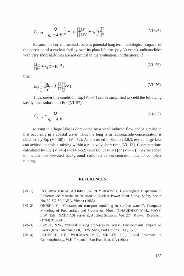
(VI–54)

Because the current method assesses potential long term radiological impacts ofthe operation of a nuclear facility over its plant lifetime (say 30 years), radionuclideswith very short half-lives are not critical to the evaluation. Furthermore, if

(VI–55)

then

(VI–56)

Thus, under this condition, Eq. (VI–54) can be simplified to yield the followingsteady state solution to Eq. (VI–57).

(VI–57)

Mixing in a large lake is dominated by a wind induced flow and is similar tothat occurring in a coastal water. Thus the long term radionuclide concentration isobtained by Eq. (VI–46) or (VI–52). As discussed in Section 4.6.3, even a large lakecan achieve complete mixing within a relatively short time [VI–13]. Concentrationscalculated by Eq. (VI–46) (or (VI–52)) and Eq. (VI–54) (or (VI–57)) may be addedto include this elevated background radionuclide concentration due to completemixing.

REFERENCES

[VI–1] INTERNATIONAL ATOMIC ENERGY AGENCY, Hydrological Dispersion ofRadionuclide Material in Relation to Nuclear Power Plant Siting, Safety SeriesNo. 50-SG-S6, IAEA, Vienna (1985).

[VI–2] ONISHI, Y., “Contaminant transport modeling in surface waters”, ComputerModeling of Free-surface and Pressurized Flows (CHAUDHRY, M.H., MAYS,L.W., Eds), NATO ASI Series E, Applied Sciences, Vol. 274, Kluwer, Dordrecht(1994) 313–341.

[VI–3] SAYRE, N.W., “Natural mixing processes in rivers”, Environmental Impact onRivers (River Mechanics II), H.W. Shen, Fort Collins, CO (1973).

[VI–4] LEOPOLD, L.B., WOLMAN, M.G., MILLER, J.P., Fluvial Processes inGeomorphology, W.H. Froeman, San Francisco, CA (1964).

CQ

q Vwr i

, tot =+ λ

exp − +

<<q

Vtr

iλ 1

q

Vr

i+

> − −λ 10 8 1s

CQ

q V

q

Vtw

r i

ri, exptot =

+− − +

λ

λ1

185

[VI–5] NATIONAL COUNCIL ON RADIATION PROTECTION ANDMEASUREMENTS, Screening Models for Releases of Radionuclides toAtmosphere, Surface Water, and Ground, Rep. No. 123 I, NCRP, Bethesda, MD(1996).

[VI–6] BOWIE, G.L., et al., Rates, Constants, and Kinetics Formulations in Surface WaterQuality Modeling, 2nd edn, prepared for the US Environmental Protection Agencyby Tetra Tech, Lafayette, CA, and Humbolt State University, Arcata, CA (1985).

[VI–7] FISHER, H.G., LIST, E.J., KOH, R.C.Y., IMBERGER, J., BROOKS, N.H., Mixingin Inland and Coastal Waters, Academic Press, San Francisco (1979).

[VI–8] HYDROSCIENCE, Simplified Mathematical Modeling of Water Quality, preparedfor the United States Environmental Protection Agency, Office of Water Programs,Washington, DC (1997).

[VI–9] WARD, P.R.B., Measurements of estuary dispersion coefficient, J. Environ. Eng.Div. 102 (1976) 855–859.

[VI–10] O’CONNER, D.J., LAWLER, J.P., Mathematical Analysis of Estuarine Pollution,55th Natl Mtg, Reprint No. 31a, American Institute of Chemical Engineers,Houston, TX (1965).

[VI–11] OKUBO, A., Oceanic diffusion diagrams, Deep-Sea Res. 18 (1971) 789–802.[VI–12] EDINGER, J.E., BUCHAK, E.M., Offshore Nuclear Dispersion and Uptake

Modeling, Appendix I: Coastal Advection and Dispersion for a Time VaryingContinuous Source with Lateral Dispersion as a Function of Distance and withRadionuclide Decay, J.E. Edinger Associates, Wayne, IN (1977).

[VI–13] UNITED STATES NUCLEAR REGULATORY COMMISSION, Liquid PathwayGeneric Study, Impacts of Accidental Radionuclide Releases to the Hydrospherefrom Floating and Land-Based Nuclear Power Plants, Rep. NUREG-0440,Washington, DC (1978).

186

187

Annex VII

METHODS USED IN THE ESTIMATION OF COLLECTIVE DOSES FORSCREENING PURPOSES

VII–1. INTRODUCTION

As discussed in Section 7, collective doses are normally estimated for aparticular location by summing the product of the number of individuals exposed andtheir average radiation dose. Models for estimating collective dose are normallyrelatively complex and are outside the scope of this report. However, estimates ofcollective dose per unit discharge have been made for use as part of the overallscreening process, as described in Section 8. These are order of magnitude estimatesonly and should be used with caution. They are based on collective doses calculatedin two different ways. The first uses complex models [VII–1], and the second is basedon simple generic models developed by UNSCEAR [VII–2]. The source of theestimates and the choice of the order of magnitude screening values are discussed inthis annex.

VII–2. THE MORE COMPLEX MODEL

A suite of mathematical models has been developed at the NationalRadiological Protection Board (NRPB) in the United Kingdom to estimate collectivedoses from releases of radionuclides to the environment [VII–1]. These modelsrepresent the transfer of radionuclides through the environment and the subsequentexposure of people. They cover dispersion over large distances and can be used tocalculate doses to the population of the United Kingdom, Europe as a whole or theworld. The models have been used to estimate collective doses from routinedischarges of radionuclides from the United Kingdom’s civil nuclear sites [VII–1]. Aswell as estimating the collective doses from actual discharges, the collective dosesfrom unit discharges of particular radionuclides were also calculated. Bothatmospheric and liquid releases were considered, and a range of values was obtainedfor the sites included in the study. It should be noted that not all radionuclides wereconsidered for each site, only those radionuclides actually discharged at the site.

Tables VII–I, VII–II and VII–III show the range of collective doses per unitdischarge given by the study for radionuclides released to the atmosphere and tomarine and freshwater bodies, respectively. In some cases the radionuclide wasdischarged from only one site, so that only one value for the collective dose can be

given. These values are the collective effective dose commitment integrated toinfinity. Collective doses truncated at 500 years are also available in Ref. [VII–1].

As seen in Table VII–I, the collective doses from atmospheric releases can havea range of more than an order of magnitude, depending on the radionuclide concernedand the location of the respective site. The highest collective doses are generallyassociated with sites located near areas of relatively high population density. Forliquid releases the range in collective doses per unit discharge may be of severalorders of magnitude depending on the radionuclides and sites concerned. The highestcollective doses are generally associated with releases from inland sites discharginginto rivers.

TABLE VII–I. COLLECTIVE EFFECTIVE DOSE COMMITMENTS PER UNITACTIVITY DISCHARGED TO THE ATMOSPHERE — DERIVATION OFVALUES FOR SCREENING PURPOSES

Simple method

Nuclide TotalContribution (%) More complex Screening

(man⋅Sv/Bq)method range value

Inhalation External External Ingestion of results (man·Sv/Bq)(cloud) (deposit)

Ac-228 1.1 × 10–12 4 0 96 0 1 × 10–12

Ag-110m 3.3 × 10–12 1 0 90 9 1 × 10–12

Am-241 1.0 × 10–10 78 0 0 22 5.7 × 10–11 – 9.6 × 10–10 1 × 10–9

Ar-41 9.6 × 10–18 – 4.1 × 10–16 1 × 10–16

As-76 6.0 × 10–13 0 0 100 0 1 × 10–12

At-211 2.5 × 10–13 81 0 18 1 1 × 10–13

Au-198 4.7 × 10–13 0 0 100 0 1 × 10–13

Bi-206 3.5 × 10–12 0 0 99 0 1 × 10–12

Bi-210 2.2 × 10–13 79 0 18 3 1 × 10–13

Bi-212 1.5 × 10–12 4 0 96 0 1 × 10–12

Br-82 2.9 × 10–12 0 0 100 0 1 × 10–12

C-14 8.6 × 10–12 – 1.1 × 10–11 1 × 10–11

Cd-109 6.6 × 10–13 2 0 4 94 1 × 10–12

Ce-141 1.3 × 10–13 5 0 62 32 1 × 10–13

Ce-144 8.4 × 10–13 12 0 24 64 9.5 × 10–14 – 2.3 × 10–13 1 × 10–12

Cm-242 1.1 × 10–11 89 0 0 11 1 × 10–11

Cm-244 6.4 × 10–11 79 0 0 21 1 × 10–10

Co-58 1.2 × 10–12 0 0 90 9 1 × 10–12

Co-60 3.7 × 10–12 2 0 71 27 2.3 × 10–12 – 2.1 × 10–11 1 × 10–11

Cr-51 3.7 × 10–14 0 0 93 7 7.5 × 10–15 1 × 10–14

Cs-134 5.6 × 10–12 0 0 31 69 2.7 × 10–12 – 9.8 × 10–12 1 × 10–11

Cs-135 3.9 × 10–13 0 0 0 100 1 × 10–13

Cs-136 2.4 × 10–12 0 0 96 4 1 × 10–12

188

TABLE VII–I. (cont.)

Simple method

Nuclide TotalContribution (%) More complex Screening

(man⋅Sv/Bq)method range value

Inhalation External External Ingestion of results (man·Sv/Bq)(cloud) (deposit)

Cs-137 3.0 × 10–12 0 0 21 79 3.0 × 10–12 – 2.4 × 10–11 1 × 10–11

Cu-64 2.1 × 10–13 0 0 100 0 1 × 10–13

Eu-154 1.7 × 10–12 6 0 81 13 1.6 × 10–12 – 1.4 × 10–11 1 × 10–11

Eu-155 1.1 × 10–13 11 0 58 31 1 × 10–13

Fe-55 4.5 × 10–14 3 0 0 97 9.7 × 10–15 – 1.8 × 10–14 1 × 10–14

Fe-59 1.4 × 10–12 1 0 89 10 4.2 × 10–13 1 × 10–12

Ga-67 1.7 × 10–13 0 0 100 0 1 × 10–13

H-3 1.3 × 10–15 – 5.0 × 10–15 1 × 10–15

Hg-197 7.3 × 10–14 1 0 99 0 1 × 10–13

Hg-197m 9.8 × 10–14 1 0 99 0 1 × 10–13

Hg-203 4.1 × 10–13 1 0 63 35 1 × 10–13

I-123 1.9 × 10–13 0 0 100 0 1 × 10–13

I-125 2.1 × 10–12 0 0 2 97 1 × 10–12

I-129 2.2 × 10–11 0 0 0 100 8.0 × 10–11 – 3.0 × 10–10 1 × 10–10

I-131 1.1 × 10–12 1 0 37 62 6.4 × 10–14 – 2.1 × 10–12 1 × 10–12

I-132 2.5 × 10–12 0 0 100 0 1 × 10–12

I-133 7.2 × 10–13 0 0 99 1 1 × 10–12

I-134 2.9 × 10–12 0 0 100 0 1 × 10–12

I-135 1.7 × 10–12 0 0 100 0 1 × 10–12

In-111 4.4 × 10–13 0 0 100 0 1 × 10–13

In-113m 2.8 × 10–13 0 0 100 0 1 × 10–13

Kr-85 2.4 × 10–17 – 4.1 × 10–17 1 × 10–17

Kr-89 2.8 × 10–17 1 × 10–17

Mn-54 9.9 × 10–13 0 0 91 8 1 × 10–12

Mo-99 3.3 × 10–13 1 0 99 1 1 × 10–13

Na-22 9.4 × 10–12 0 0 25 75 1 × 10–11

Na-24 4.1 × 10–12 0 0 100 0 1 × 10–12

Nb-95 8.7 × 10–13 0 0 95 4 2.3 × 10–14 – 6.6 × 10–14 1 × 10–12

Ni-59 2.4 × 10–13 0 0 0 100 1 × 10–13

Ni-63 5.4 × 10–13 0 0 0 100 1 × 10–12

Np-237 5.6 × 10–11 77 0 0 23 1 × 10–10

Np-239 1.8 × 10–13 1 0 99 0 1 × 10–13

P-32 3.1 × 10–13 2 0 30 68 6.4 × 10–13 – 9.0 × 10–13 1 × 10–12

Pa-231 3.4 × 10–10 76 0 0 24 1 × 10–10

Pa-233 2.7 × 10–13 3 0 80 17 1 × 10–13

Pb-210 8.6 × 10–11 2 0 0 98 1 × 10–10

Pd-103 2.2 × 10–14 4 0 65 31 1 × 10–14

Pd-107 8.2 × 10–15 13 0 0 87 1 × 10–14

Pd-109 4.5 × 10–14 2 0 98 0 1 × 10–14

Pm-147 3.8 × 10–14 25 0 0 75 1 × 10–14

Po-210 1.3 × 10–10 1 0 0 99 1 × 10–10

189

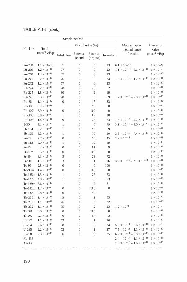
TABLE VII–I. (cont.)

Simple method

Nuclide TotalContribution (%) More complex Screening

(man⋅Sv/Bq)method range value

Inhalation External External Ingestion of results (man·Sv/Bq)(cloud) (deposit)

Pu-238 1.1 × 10–10 77 0 0 23 6.1 × 10–10 1 × 10–9Pu-239 1.2 × 10–10 77 0 0 23 1.1 × 10–10 – 6.6 × 10–10 1 × 10–9

Pu-240 1.2 × 10–10 77 0 0 23 1 × 10–10

Pu-241 2.2 × 10–12 76 0 0 24 1.9 × 10–12 – 1.2 × 10–11 1 × 10–11

Pu-242 1.2 × 10–10 77 0 0 23 1 × 10–10

Ra-224 8.2 × 10–12 78 0 20 2 1 × 10–11

Ra-225 1.8 × 10–11 80 0 2 19 1 × 10–11

Ra-226 6.3 × 10–11 28 0 3 69 1.7 × 10–10 – 2.8 × 10–10 1 × 10–10

Rb-86 1.1 × 10–12 0 0 17 83 1 × 10–12

Rh-105 8.7 × 10–14 1 0 99 0 1 × 10–13

Rh-107 3.9 × 10–13 0 0 100 0 1 × 10–13

Ru-103 5.8 × 10–13 1 0 89 10 1 × 10–12

Ru-106 1.4 × 10–12 9 0 28 63 1.6 × 10–13 – 4.2 × 10–13 1 × 10–12

S-35 2.1 × 10–13 1 0 0 99 3.1 × 10–13 – 2.0 × 10–12 1 × 10–12

Sb-124 2.2 × 10–12 1 0 90 9 1 × 10–12

Sb-125 6.2 × 10–13 1 0 79 20 2.6 × 10–13 – 7.4 × 10–13 1 × 10–12

Se-75 7.7 × 10–13 0 0 55 45 2.2 × 10–11 1 × 10–11

Sn-113 3.9 × 10–13 1 0 79 19 1 × 10–13

Sr-85 6.2 × 10–13 0 0 91 9 1 × 10–12

Sr-87m 3.5 × 10–13 0 0 100 0 1 × 10–13

Sr-89 3.3 × 10–13 5 0 23 72 1 × 10–13

Sr-90 1.1 × 10–11 3 0 1 96 3.2 × 10–12 – 2.3 × 10–11 1 × 10–11

Tc-99 2.8 × 10–13 0 0 0 100 1 × 10–13

Tc-99m 1.4 × 10–13 0 0 100 0 1 × 10–13

Te-125m 1.5 × 10–13 1 0 27 73 1 × 10–13

Te-127m 4.0 × 10–13 1 0 6 93 1 × 10–13

Te-129m 3.6 × 10–13 1 0 19 81 1 × 10–13

Te-131m 1.7 × 10–12 0 0 100 0 1 × 10–12

Te-132 2.8 × 10–12 0 0 99 1 1 × 10–12

Th-228 1.4 × 10–10 43 0 1 55 1 × 10–10

Th-230 1.1 × 10–10 76 0 2 22 1 × 10–10

Th-232 1.1 × 10–10 75 0 2 23 1.2 × 10–9 1 × 10–9

Tl-201 9.8 × 10–14 0 0 100 0 1 × 10–13

Tl-202 5.3 × 10–13 0 0 97 3 1 × 10–12

U-232 1.1 × 10–10 62 0 1 36 1 × 10–10

U-234 2.6 × 10–11 68 0 8 24 5.6 × 10–11 – 5.6 × 10–10 1 × 10–9

U-235 2.2 × 10–11 72 0 1 27 7.5 × 10–11 – 1.1 × 10–10 1 × 10–10

U-238 2.3 × 10–11 66 0 9 25 6.2 × 10–11 – 8.8 × 10–11 1 × 10–10

Xe-133 2.4 × 10–17 – 1.1 × 10–16 1 × 10–16

Xe-135 7.9 × 10–18 – 1.6 × 10–16 1 × 10–16

190

TABLE VII–I. (cont.)

Simple method

Nuclide TotalContribution (%) More complex Screening

(man⋅Sv/Bq)method range value

Inhalation External External Ingestion of results (man·Sv/Bq)(cloud) (deposit)

Y-87 8.5 × 10–13 0 0 100 0 1 × 10–12

Y-90 1.3 × 10–13 2 0 97 1 1 × 10–13

Y-91 2.9 × 10–13 6 0 28 66 1 × 10–13

Zn-65 1.8 × 10–12 0 0 34 65 5.1 × 10–12 – 2.0 × 10–11 1 × 10–11

Zr-95 1.7 × 10–12 1 0 95 4 8.2 × 10–14 – 2.3 × 10–13 1 × 10–12

TABLE VII–II. COLLECTIVE EFFECTIVE DOSE COMMITMENTS PER UNITACTIVITY DISCHARGED INTO MARINE WATERS — DERIVATION OFVALUES FOR SCREENING PURPOSES

Simple method

Nuclide TotalContribution (%) More complex Screening

(man·Sv/Bq)method range value

Fish Shellfish of results (man·Sv/Bq)ingestion ingestion

Ac-228 2.4 × 10–18 23 77 1 × 10–18

Ag-110m 1.2 × 10–13 23 77 1.6 × 10–13 – 2.6 × 10–13 1 × 10–13

Am-241 2.5 × 10–12 1 99 2.6 × 10–14 – 6.2 × 10–14 1 × 10–13

As-76 2.4 × 10–16 75 25 1 × 10–16

At-211 6.2 × 10–18 55 45 1 × 10–17

Au-198 7.3 × 10–17 38 63 1 × 10–16

Bi-206 2.2 × 10–16 11 89 1 × 10–16

Bi-210 1.2 × 10–16 11 89 1 × 10–16

Bi-212 2.1 × 10–19 11 89 1 × 10–19

Br-82 3.8 × 10–19 64 36 1 × 10–19

C-14 9.8 × 10–12 – 1.1 × 10–11 1 × 10–11

Cd-109 2.5 × 10–13 23 77 1 × 10–13

Ce-141 9.5 × 10–17 6 94 5.9 × 10–17 1 × 10–16

Ce-144 4.6 × 10–15 6 94 2.2 × 10–16 – 5.4 × 10–15 1 × 10–14

Cm-242 3.9 × 10–14 1 99 1.9 × 10–15 – 6.2 × 10–14 1 × 10–13

Cm-244 2.0 × 10–12 1 99 2.8 × 10–14 – 1.4 × 10–12 1 × 10–12

Co-58 3.0 × 10–15 55 45 9.1 × 10–16 – 4.9 × 10–15 1 × 10–15

Co-60 1.2 × 10–13 55 45 1.3 × 10–14 – 7.3 × 10–14 1 × 10–13

Cr-51 3.7 × 10–17 75 25 7.3 × 10–18 – 3.9 × 10–17 1 × 10–17

191

TABLE VII–II. (cont.)

Simple method

Nuclide TotalContribution (%) More complex Screening

(man·Sv/Bq)method range value

Fish Shellfish of results (man·Sv/Bq)ingestion ingestion

Cs-134 7.5 × 10–14 95 5 1.3 × 10–14 – 5.2 × 10–14 1 × 10–13

Cs-135 1.6 × 10–14 95 5 1 × 10–14

Cs-136 4.0 × 10–16 95 5 1 × 10–16

Cs-137 9.6 × 10–14 95 5 1.3 × 10–14 – 5.6 × 10–14 1 × 10–13

Cu-64 6.7 × 10–18 68 32 1 × 10–17

Eu-154 3.1 × 10–14 20 80 4.2 × 10–15 – 3.1 × 10–14 1 × 10–14

Eu-155 7.8 × 10–16 38 63 3.5 × 10–16 – 2.7 × 10–15 1 × 10–15

Fe-55 7.7 × 10–14 38 63 3.6 × 10–15 – 5.0 × 10–14 1 × 10–13

Fe-59 4.1 × 10–14 38 63 9.9 × 10–15 – 7.1 × 10–14 1 × 10–13

Ga-67 5.1 × 10–17 86 14 1 × 10–16

H-3 3.2 × 10–18 – 3.8 × 10–18 1 × 10–18

Hg-197 1.5 × 10–15 86 14 1 × 10–15

Hg-197m 1.1 × 10–15 86 14 1 × 10–15

Hg-203 2.0 × 10–13 86 14 1 × 10–13

I-123 1.4 × 10–19 86 14 1 × 10–19

I-125 9.9 × 10–16 86 14 3.0 × 10–16 1 × 10–16

I-129 9.9 × 10–14 86 14 6.3 × 10–15 – 4.7 × 10–11 1 × 10–11

I-131 2.1 × 10–16 86 14 1 × 10–16

I-132 3.3 × 10–20 86 14 1 × 10–20

I-133 4.4 × 10–18 86 14 1 × 10–18

I-134 4.8 × 10–21 86 14 1 × 10–21

I-135 3.0 × 10–19 86 14 1 × 10–19

In-111 2.2 × 10–16 38 63 1 × 10–16

In-113m 5.3 × 10–19 38 63 1 × 10–18

Mn-54 6.6 × 10–15 32 68 9.7 × 10–16 – 6.7 × 10–15 1 × 10–14

Mo-99 4.5 × 10–18 38 63 1 × 10–18

Na-22 2.1 × 10–17 67 33 1 × 10–17

Na-24 4.1 × 10–21 67 33 1 × 10–21

Nb-95 3.9 × 10–16 15 85 1.2 × 10–17 – 4.2 × 10–16 1 × 10–16

Ni-59 6.5 × 10–15 75 25 1 × 10–14

Ni-63 1.5 × 10–14 75 25 2.0 × 10–16 – 3.8 × 10–15 1 × 10–15

Np-237 3.2 × 10–13 13 87 1.6 × 10–12 – 1.8 × 10–12 1 × 10–12

Np-239 1.4 × 10–17 13 87 1 × 10–17

P-32 1.1 × 10–13 90 10 2.2 × 10–14 – 1.5 × 10–13 1 × 10–13

Pa-231 7.3 × 10–12 38 63 1 × 10–11

Pa-233 3.1 × 10–16 38 63 1 × 10–16

Pb-210 1.8 × 10–11 55 45 1 × 10–11

192

TABLE VII–II. (cont.)

Simple method

Nuclide TotalContribution (%) More complex Screening

(man·Sv/Bq)method range value

Fish Shellfish of results (man·Sv/Bq)ingestion ingestion

Pd-103 1.1 × 10–16 86 14 1 × 10–16

Pd-107 1.0 × 10–15 86 14 1 × 10–15

Pd-109 1.1 × 10–17 86 14 1 × 10–17

Pm-147 7.1 × 10–16 38 63 1.0 × 10–17 – 5.7 × 10–16 1 × 10–15

Po-210 1.5 × 10–10 19 81 1 × 10–10

Pu-238 4.7 × 10–12 7 93 1.2 × 10–13 – 2.4 × 10–12 1 × 10–12

Pu-239 5.2 × 10–12 7 93 1.6 × 10–13 – 3.8 × 10–12 1 × 10–12

Pu-240 5.2 × 10–12 7 93 1 × 10–11

Pu-241 8.8 × 10–14 7 93 2.6 × 10–15 – 5.4 × 10–14 1 × 10–13

Pu-242 5.0 × 10–12 7 93 1 × 10–12

Ra-224 1.5 × 10–14 75 25 1 × 10–14

Ra-225 9.3 × 10–14 75 25 1 × 10–13

Ra-226 1.4 × 10–11 75 25 1 × 10–11

Rb-86 5.4 × 10–16 97 3 1 × 10–15

Rh-105 1.5 × 10–17 38 63 1 × 10–17

Rh-107 9.8 × 10–21 38 63 1 × 10–20

Ru-103 9.3 × 10–16 1 99 7.2 × 10–17 – 6.0 × 10–16 1 × 10–15

Ru-106 5.9 × 10–14 1 99 2.9 × 10–15 – 1.3 × 10–13 1 × 10–13

S-35 1.6 × 10–17 75 25 1.3 × 10–18 – 3.4 × 10–17 1 × 10–17

Sb-124 6.6 × 10–15 86 14 2.0 × 10–15 – 8.7 × 10–15 1 × 10–14

Sb-125 2.2 × 10–14 86 14 6.1 × 10–15 – 3.1 × 10–14 1 × 10–14

Se-75 1.9 × 10–13 86 14 1 × 10–13

Sr-85 7.9 × 10–18 86 14 1 × 10–17

Sr-87m 8.2 × 10–22 86 14 1 × 10–21

Sr-89 2.9 × 10–17 86 14 8.8 × 10–18 – 4.0 × 10–17 1 × 10–17

Sr-90 4.7 × 10–15 86 14 5.7 × 10–16 – 2.7 × 10–15 1 × 10–15

Tc-99 9.7 × 10–15 15 85 1.7 × 10–14 – 2.0 × 10–14 1 × 10–14

Tc-99m 1.1 × 10–19 15 85 1 × 10–19

Te-125m 5.6 × 10–15 86 14 1.0 × 10–15 – 7.0 × 10–15 1 × 10–14

Te-127m 2.6 × 10–14 86 14 1 × 10–14

Te-129m 1.1 × 10–14 86 14 1 × 10–14

Te-131m 2.8 × 10–16 86 14 1 × 10–16

Te-132 1.5 × 10–15 86 14 1 × 10–15

Th-228 9.7 × 10–13 78 22 6.3 × 10–15 1 × 10–14

Th-230 5.9 × 10–13 78 22 3.3 × 10–14 1 × 10–14

Th-232 6.5 × 10–13 78 22 9.3 × 10–15 1 × 10–14

Tl-201 1.7 × 10–16 86 14 1 × 10–16

193

TABLE VII–II. (cont.)

Simple method

Nuclide TotalContribution (%) More complex Screening

(man·Sv/Bq)method range value

Fish Shellfish of results (man·Sv/Bq)ingestion ingestion

Tl-202 3.2 × 10–15 86 14 1 × 10–15

U-232 1.5 × 10–13 17 83 1 × 10–13

U-234 2.3 × 10–14 17 83 9.4 × 10–14 – 1.2 × 10–13 1 × 10–13

U-235 2.2 × 10–14 17 83 9.2 × 10–14 – 1.1 × 10–13 1 × 10–13

U-238 2.1 × 10–14 17 83 8.6 × 10–14 – 1.1 × 10–13 1 × 10–13

Y-87 3.5 × 10–17 11 89 1 × 10–17

Y-90 1.4 × 10–16 11 89 4.6 × 10–19 – 1.6 × 10–17 1 × 10–17

Y-91 2.5 × 10–15 11 89 1.1 × 10–17 – 5.7 × 10–17 1 × 10–16

Zn-65 5.7 × 10–13 11 89 5.9 × 10–14 – 6.3 × 10–13 1 × 10–12

Zr-95 4.4 × 10–16 2 98 6.4 × 10–17 – 1.53 × 10–15 1 × 10–15

194

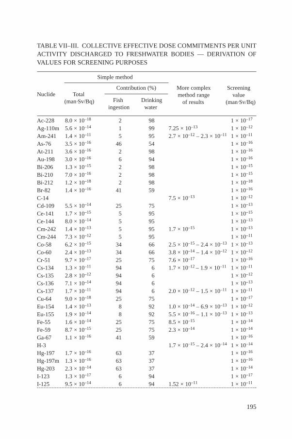
TABLE VII–III. COLLECTIVE EFFECTIVE DOSE COMMITMENTS PER UNITACTIVITY DISCHARGED TO FRESHWATER BODIES — DERIVATION OFVALUES FOR SCREENING PURPOSES

Simple method

Nuclide TotalContribution (%) More complex Screening

(man·Sv/Bq)method range value

Fish Drinking of results (man·Sv/Bq)ingestion water

Ac-228 8.0 × 10–18 2 98 1 × 10–17

Ag-110m 5.6 × 10–14 1 99 7.25 × 10–13 1 × 10–12

Am-241 1.4 × 10–11 5 95 2.7 × 10–12 – 2.3 × 10–11 1 × 10–11

As-76 3.5 × 10–16 46 54 1 × 10–16

At-211 3.6 × 10–16 2 98 1 × 10–16

Au-198 3.0 × 10–16 6 94 1 × 10–16

Bi-206 1.3 × 10–15 2 98 1 × 10–15

Bi-210 7.0 × 10–16 2 98 1 × 10–15

Bi-212 1.2 × 10–18 2 98 1 × 10–18

Br-82 1.4 × 10–16 41 59 1 × 10–16

C-14 7.5 × 10–13 1 × 10–12

Cd-109 5.5 × 10–14 25 75 1 × 10–13

Ce-141 1.7 × 10–15 5 95 1 × 10–15

Ce-144 8.0 × 10–14 5 95 1 × 10–13

Cm-242 1.4 × 10–13 5 95 1.7 × 10–15 1 × 10–13

Cm-244 7.3 × 10–12 5 95 1 × 10–11

Co-58 6.2 × 10–15 34 66 2.5 × 10–15 – 2.4 × 10–13 1 × 10–13

Co-60 2.4 × 10–13 34 66 3.8 × 10–14 – 1.4 × 10–12 1 × 10–12

Cr-51 9.7 × 10–17 25 75 7.6 × 10–17 1 × 10–16

Cs-134 1.3 × 10–11 94 6 1.7 × 10–12 – 1.9 × 10–11 1 × 10–11

Cs-135 2.8 × 10–12 94 6 1 × 10–12

Cs-136 7.1 × 10–14 94 6 1 × 10–13

Cs-137 1.7 × 10–11 94 6 2.0 × 10–12 – 1.5 × 10–11 1 × 10–11

Cu-64 9.0 × 10–18 25 75 1 × 10–17

Eu-154 1.4 × 10–13 8 92 1.0 × 10–14 – 6.9 × 10–13 1 × 10–12

Eu-155 1.9 × 10–14 8 92 5.5 × 10–16 – 1.1 × 10–13 1 × 10–13

Fe-55 1.6 × 10–14 25 75 8.5 × 10–15 1 × 10–14

Fe-59 8.7 × 10–15 25 75 2.3 × 10–14 1 × 10–14

Ga-67 1.1 × 10–16 41 59 1 × 10–16

H-3 1.7 × 10–15 – 2.4 × 10–14 1 × 10–14

Hg-197 1.7 × 10–16 63 37 1 × 10–16

Hg-197m 1.3 × 10–16 63 37 1 × 10–16

Hg-203 2.3 × 10–14 63 37 1 × 10–14

I-123 1.3 × 10–17 6 94 1 × 10–17

I-125 9.5 × 10–14 6 94 1.52 × 10–11 1 × 10–11

195

TABLE VII–III. (cont.)

Simple method

Nuclide TotalContribution (%) More complex Screening

(man·Sv/Bq)method range value

Fish Drinking of results (man·Sv/Bq)ingestion water

I-129 9.5 × 10–12 6 94 1 × 10–11

I-131 2.0 × 10–14 6 94 7.3 × 10–12 1 × 10–11

I-132 3.2 × 10–18 6 94 1 × 10–18

I-133 4.2 × 10–16 6 94 1 × 10–16

I-134 4.6 × 10–19 6 94 1 × 10–19

I-135 2.9 × 10–17 6 94 1 × 10–17

In-111 1.5 × 10–15 94 6 1 × 10–15

In-113m 3.6 × 10–18 94 6 1 × 10–18

Mn-54 2.7 × 10–14 41 59 2.9 × 10–17 – 5.3 × 10–15 1 × 10–14

Mo-99 1.2 × 10–16 2 98 1 × 10–16

Na-22 1.4 × 10–13 3 97 1 × 10–13

Na-24 2.8 × 10–17 3 97 1 × 10–17

Nb-95 6.3 × 10–18 34 66 1.3 × 10–13 1 × 10–13

Ni-59 4.0 × 10–15 15 85 1 × 10–15

Ni-63 9.3 × 10–15 15 85 1.3 × 10–14 1 × 10–14

Np-237 4.7 × 10–12 5 95 1 × 10–12

Np-239 2.1 × 10–16 5 95 1 × 10–16

P-32 3.1 × 10–13 99 1 3.3 × 10–13 – 2.3 × 10–12 1 × 10–12

Pa-231 4.7 × 10–11 2 98 1 × 10–11

Pa-233 2.0 × 10–15 2 98 1 × 10–15

Pb-210 5.2 × 10–11 34 66 1 × 10–10

Pd-103 2.3 × 10–16 2 98 1 × 10–16

Pd-107 2.0 × 10–15 2 98 1 × 10–15

Pd-109 2.2 × 10–17 2 98 1 × 10–17

Pm-147 9.9 × 10–15 5 95 1 × 10–14

Po-210 1.1 × 10–11 8 92 1 × 10–11

Pu-238 3.2 × 10–12 5 95 3.3 × 10–13 1 × 10–12

Pu-239 3.5 × 10–12 5 95 1.1 × 10–10 1 × 10–12

Pu-240 3.5 × 10–12 5 95 1 × 10–12

Pu-241 6.0 × 10–14 5 95 9.0 × 10–14 1 × 10–13

Pu-242 3.4 × 10–12 5 95 1 × 10–12

Ra-224 2.7 × 10–14 8 92 1 × 10–14

Ra-225 1.6 × 10–13 8 92 1 × 10–13

Ra-226 2.4 × 10–11 8 92 3.7 × 10–10 – 4.0 × 10–10 1 × 10–10

Rb-86 2.3 × 10–14 77 23 1 × 10–14

Rh-105 4.7 × 10–17 2 98 1 × 10–17

Rh-107 3.1 × 10–20 2 98 1 × 10–20

196

TABLE VII–III. (cont.)

Simple method

Nuclide TotalContribution (%) More complex Screening

(man·Sv/Bq)method range value

Fish Drinking of results (man·Sv/Bq)ingestion water

Ru-103 2.9 × 10–15 2 98 4.8 × 10–13 1 × 10–13

Ru-106 1.8 × 10–13 2 98 1.2 × 10–14 – 6.3 × 10–12 1 × 10–11

S-35 1.3 × 10–14 58 42 9.9 × 10–14 – 8.5 × 10–13 1 × 10–12

Sb-124 1.7 × 10–14 15 85 4.9 × 10–15 1 × 10–14

Sb-125 5.9 × 10–14 15 85 1.6 × 10–14 – 1.6 × 10–12 1 × 10–12

Se-75 3.8 × 10–14 25 75 1 × 10–14

Sr-85 3.8 × 10–15 11 89 1 × 10–15

Sr-87m 4.0 × 10–19 11 89 1 × 10–19

Sr-89 1.4 × 10–14 11 89 1.6 × 10–13 – 2.8 × 10–12 1 × 10–12

Sr-90 2.3 × 10–12 11 89 7.5 × 10–13 – 3.5 × 10–11 1 × 10–11

Tc-99 5.4 × 10–14 3 97 1 × 10–13

Tc-99m 6.1 × 10–19 3 97 1 × 10–18

Te-125m 8.4 × 10–15 41 59 1 × 10–14

Te-127m 3.9 × 10–14 41 59 1 × 10–14

Te-129m 1.7 × 10–14 41 59 1 × 10–14

Te-131m 4.2 × 10–16 41 59 1 × 10–16

Te-132 2.2 × 10–15 41 59 1 × 10–15

Th-228 2.2 × 10–11 15 85 1 × 10–11

Th-230 1.3 × 10–11 15 85 1 × 10–11

Th-232 1.5 × 10–11 15 85 1 × 10–11

Tl-201 5.5 × 10–17 63 37 1 × 10–16

Tl-202 1.0 × 10–15 63 37 1 × 10–15

U-232 2.6 × 10–11 2 98 1 × 10–11

U-234 4.0 × 10–12 2 98 1.42 × 10–10 1 × 10–10

U-235 3.9 × 10–12 2 98 1 × 10–12

U-238 3.7 × 10–12 2 98 7.7 × 10–11 1 × 10–10

Y-87 1.7 × 10–16 5 95 1 × 10–16

Y-90 6.7 × 10–16 5 95 6.2 × 10–17 1 × 10–15

Y-91 1.2 × 10–14 5 95 1 × 10–14

Zn-65 2.0 × 10–13 63 37 6.3 × 10–13 – 5.0 × 10–12 1 × 10–12

Zr-95 8.6 × 10–15 34 66 2.1 × 10–14 1 × 10–14

197

VII–3. SIMPLE GENERIC MODEL

UNSCEAR has developed a set of simple generic models that can be used toestimate collective doses for the transfer of radionuclides in the environment withoutusing complex models [VII–2]. Generic global parameter values can be used withthese models if site specific data are not available.

For atmospheric releases it is assumed that all the activity released will bedeposited and that the collective dose is independent of the distribution pattern of thedeposited material. Three exposure pathways were considered here: inhalation,ingestion of terrestrial foods and external radiation from deposited material. Apopulation density is required in this calculation of collective dose; for the purposesof calculating screening values a population density of 35 people per km2 was used[VII–3]. This represents a global average; considerably higher densities can be foundin some countries, while lower densities can be found in others. Global average yieldsof particular foods were also required and were obtained from an FAO compilation[VII–3]. The foods considered were grain, green vegetables and fruit, root vegetables,milk and meat.

Table VII–I gives values of the collective doses for unit releases of variousradionuclides to the atmosphere estimated using a simplified method based on theUNSCEAR approach. These are the collective effective dose commitment valuescalculated using the effective dose coefficients given in Section 6 of this report. Inmost cases the values are of the same order as, or in the range of, the collective dosesobtained from the more complex models, and are also presented in Table VII–I.

For releases of radionuclides in liquid form their dispersion and subsequenttransfer to humans will vary considerably depending on the characteristics of thereceiving water body. In the general model developed by UNSCEAR [VII–2], simpledilution is assumed. Account is taken of the transfer of radionuclides to sedimentsthrough the use of the sediment distribution coefficient Kd . The exposure pathwaysconsidered are the consumption of drinking water and aquatic foods; in thisapplication fish and crustacea were considered. It is assumed that the number ofpeople consuming the food divided by the volume of the receiving waters is relativelyconstant, and generic values of 4.3 × 10–9 and 4.6 × 10–8 people/L for marine andfresh waters, respectively [VII–2], are used. The collective doses obtained usingthis method are given in Tables VII–II and VII–III and were obtained using theeffective dose coefficients given in Section 6. In some cases there are significantdifferences between the generic results and those obtained using the more complexmodel. In these cases generally the more complex model was applied toradionuclides discharged into coastal waters, where a much lower value of the ratiobetween the number of people consuming seafood and the volume of the receivingwaters applies.

198

VII–4. CHOICE OF SCREENING VALUES

The collective doses given in Tables VII–I to VII–III were used to obtain orderof magnitude estimates of collective doses per unit discharge to be used for screeningpurposes. These estimates are also presented in the tables. In many cases the genericvalue and the range obtained from the more complex method were of the same orderof magnitude, making the choice of screening value straightforward. However, inother cases there was a considerable range in the values obtained; in these cases anorder of magnitude at the top of the range was chosen. In addition, where differentradionuclides were expected to have collective doses of the same order of magnitude,for example 238Pu and 239Pu, the order of magnitude estimates were made to be thesame even if the range available did not indicate this. Because of the methods used todetermine the order of magnitude estimates, these should be used with extremecaution and only for screening purposes.

REFERENCES

[VII–1] BEXON, A.P., Radiological Impact of Routine Discharges from UK Civil NuclearSites in the Mid 1990s, Rep. NRPB-R312, National Radiological Protection Board,Chilton (1999).

[VII–2] UNITED NATIONS, Dose Assessment Methodologies, Draft R602, ScientificCommittee on the Effects of Atomic Radiation (UNSCEAR), UN, New York (1999).

[VII–3] FOOD AND AGRICULTURE ORGANIZATION OF THE UNITED NATIONS,FAO Production Yearbook 1980, Vol. 34, FAO, Rome (1981).

199

201

SYMBOLS FOR PARAMETERS USED IN THIS REPORT

SECTION 3

Symbol Unit Description

AB m2 Projected cross-sectional area of the building mostinfluencing the flow of the plume.

B m–2 Gaussian diffusion factor corrected for dispersion inthe lee of a building inside the wake zone (use insteadof F).

B0 – Unitless constant that accounts for the potentialincrease in air concentration along a vertical wall.

CA Bq/m3 Annual average concentration of radionuclide in air(at ground level).

d◊ i Bq·m–2·d–1 Daily average deposition rate to the ground surface ofradionuclide i from both dry and wet processes.

E, G — Fit parameters for the equation that defines sz.

f — Unitless reduction factor accounting for radioactivedecay during atmospheric transport.

F m–2 Gaussian diffusion factor appropriate for the height ofrelease H and downwind distance x.

K m Constant with a value of 1 m.

H m Height at which the radionuclide is released.

HB m Height of the building that dominates the air flow nearthe radionuclide release point.

Pp — Fraction of time during the year that the wind blowstowards the receptor of interest in sector p.

Qi Bq/s Annual average rate of radionuclide emission to theatmosphere.

ua m/s Annual geometric mean of the wind speed at theheight of the release.

V m3/s Volumetric flow rate of vent or stack at the point ofrelease.

Vd m/d Dry deposition coefficient (deposition on to soil andvegetation).

Vw m/d Wet deposition coefficient.

VT m/d Total (dry and wet) deposition coefficient.

x m Location of the receptor (downwind distance).

li s–1 Radioactive decay constant for radionuclide i.

sz m Vertical diffusion parameter.

SECTION 4

Symbol Unit Description

B m River or estuary width.

B–

m River width under a mean annual river flow rateupstream of the tidal flow area.

C0 Bq/m3 Radionuclide concentration in water at the effluentdischarge outfall.

Cs,b Bq/kg Radionuclide concentration in bottom sediment.

Cs,s Bq/m2 Radionuclide concentration in shore or beachsediment.

Cs,w Bq/kg Radionuclide concentration in suspended sediment.

Cte Bq/m3 Maximum radionuclide concentration on the riverbank opposite to the discharge point.

Csludge Bq/kg Annual average radionuclide concentration in sewagesludge.

Cw,s Bq/m3 Radionuclide concentration in filtered water.

Cw, tot Bq/m3 Total radionuclide concentration in water.

D m Flow depth that corresponds to qr.

F m3/s Flow rate of the liquid effluent.

Kd L/kg Distribution coefficient between the radionuclide onsediment and that dissolved in water.

202

Pr — Correction factor for partial mixing.

qr m3/s 30 year low annual river flow rate.

qr m3/s Mean annual river flow rate.

Qi Bq/s Average radionuclide discharge rate into river, estuary,lake or coastal waters.

Qsludge Bq/a Annual discharge of a radionuclide to a sewage plant.

Ssludge kg/a Annual sewage sludge production at the relevantsewage treatment works.

Ss kg/m3 or g/L Suspended sediment concentration.

Te s Effective accumulation time for shore or beachsediment.

Tp s Tidal period.

U m/s Net freshwater velocity.

x m Longitudinal distance from the release point to apotential receptor location.

y0 m Distance between the release point and the beach.

li s–1 Radionuclide decay constant for radionuclide i.

SECTION 5

Symbol Unit Description

Bp L/kg Equilibrium ratio of the concentration of a radionuclidein aquatic food p to its dissolved concentration inwater, known as the bioaccumulation factor.

Bv Bq/kgplant tissue Concentration factor for the uptake of radionuclide per Bq/kgdry soil from soil by edible parts of crops; adhesion of soil to

the vegetation is not taken into account. For pasturegrass the unit of mass is dry matter; for vegetablesconsumed by humans it is fresh weight.

CA Bq/m3air Annual average concentration of radionuclide in air.

Ca,i Bq/kgdry weight Annual average concentration of radionuclide in animalfeed.

203

Caf,i Bq/kg Annual average concentration of radionuclide inaquatic foods.

Cf,i Bq/kgmeat Annual average concentration of radionuclide in meat.

Cm,i Bq/Lmilk Annual average concentration of radionuclide in milk.

Cp,i Bq/kgdry matter Annual average concentration of radionuclide instored animal feed.

Cs Bq/kg Annual average concentration of radionuclide in drysoil.

Cv,i Bq/kg Annual average concentration of radionuclide in foodcrops (expressed in fresh matter for vegetationconsumed by humans and in dry matter for vegetationconsumed by animals).

Cw,i Bq/Lwater Annual average concentration in water.

d·i Bq·m–2·d–1 Annual average deposition rate from wet and dry

processes to the ground surface.

Ff d/kgmeat Fraction of the animal daily intake that appears in akilogram of flesh at the time of slaughter.

Fm d/Lmilk Fraction of animal daily intake that appears in a litreof milk at the time of milking.

fp — Fraction of time during a year that an animalconsumes fresh pasture.

Fv Bq/kgplant tissue Concentration factor for the uptake of radionuclide per Bq/kgdry soil from soil by edible parts of crops, adjusted implicitly

to account for adhesion of soil to the vegetation. Forpasture grass the unit of mass is dry matter; forvegetables consumed by humans it is fresh weight.

Iw m3water·m

–2·d–1 Average irrigation rate.

Qf kgdry matter/d Amount of feed consumed per day by a meatproducing animal.

Qm kgdry matter/d Amount of feed consumed per day by a milkproducing animal.

Qw m3/d Amount of water consumed per day by an animal.

tb d Duration of discharge of radioactive material.

204

te d Time period that crops are exposed to contaminationduring the growing season.

tf d Time interval between slaughter and consumption ofthe meat.

th d Delay (holdup) time that represents the time intervalbetween harvest and consumption of the food.

tm d Time interval between milking and consumption ofthe milk.

a m2/kg Mass interception fraction for a given food crop.

lEsi

d–1 Effective rate constant responsible for reductioradionuclide concentration in the root zo

lEvi

d–1 Effective rate constant responsible for reduction of theradionuclide concentration on vegetation.

li d–1 Radioactive decay constant of a radionuclide.

lw d–1 Effective rate constant responsible for reduction of theconcentration of material deposited on plant surfacesdue to processes other than radioactive decay.

ls d–1 Effective rate constant responsible for reduction of theconcentration of material deposited in the root zone ofsoils due to processes other than radioactive decay.

r kg/m2dry soil Effective surface soil density for the root zone.

SECTION 6

Symbol Unit Description

CA Bq/m3 Annual average concentration in air.

Cgr Bq/m2 Ground surface concentration resulting from a 30 yeardischarge to the atmosphere.

Cp,i Bq/kg Concentration of radionuclide i in foodstuff p at thetime of consumption.

Cs,s Bq/m2 Annual average sediment surface concentration.

205

Csludge Bq/kg Mass concentration deposited in sewage sludge.

Csludge Bq/m2 Surface concentration deposited in sewage sludge.

DFs Sv/a per Bq/m3 Dose coefficient for skin from air immersion.

DFgr Sv/a per Bq/m2 Dose coefficient for exposure to contaminated groundor sediment surfaces.

DFim Sv/a per Bq/m3 Immersion dose coefficient.

DFing Sv/Bq Dose coefficient for ingestion of radionuclides.

DFinh Sv/Bq Dose coefficient for inhalation of radionuclides.

DL kg/m3 Dust loading factor.

Egr Sv/a External dose rate from ground deposits after a 30year discharge to the atmosphere.

Einh Sv/a Annual inhalation dose from the concentration in air.

Eim Sv/a External dose rate from immersion in a dischargecloud.

Eim, s Sv/a External dose rate to skin from immersion in adischarge cloud.

Eing, p Sv/a Annual dose from ingestion of foodstuff p.

Em Sv/a External dose rate from exposure to contaminatedsediment.

Eres Sv/a Annual inhalation dose from resuspension ofradionuclides deposited in sewage sludge.

Es Sv/a External dose rate from concentration in sewagesludge.

Hp kg/a Annual average consumption rate for foodstuff p.

Of — Fraction of time in a year when an individual isexposed to a particular exposure pathway.

Rinh m3/a Annual average inhalation rate.

r kg/m3 Density (in Section 6 the density of sewage sludge isreferred to).

206

207

GLOSSARY

critical group. A group of members of the public which is reasonably homogeneouswith respect to its exposure for a given radiation source and given exposurepathway and is typical of individuals receiving the highest effective dose orequivalent dose (as applicable) from the given source.

decay constant, ll . For a radionuclide in a particular energy state the quotient of dPby dt, where dP is the probability of a given nucleus undergoing a spontaneousnuclear transition from that energy state in the time interval dt.

discharge. Planned and controlled release of (usually gaseous or liquid) radioactivematerial to the environment.

authorized discharge: discharge in accordance with an authorization.

dispersion. The spreading of radionuclides in air (aerodynamic dispersion) or water(hydrodynamic dispersion) resulting mainly from physical processes affectingthe velocity of different molecules in the medium.

dose. A measure of the energy deposited by radiation in a target.∑ For definitions of the most important such measures, see dose quantities

and dose concepts.

dose concepts.

annual dose: the dose due to external exposure in a year plus the committeddose from intakes of radionuclides in that year.

collective dose: the total radiation dose incurred by a population.∑ This is the sum of all of the individual doses to members of this population.

If the doses continue for longer than a year, then the annual individualdoses must also be integrated over time. Unless otherwise specified, thetime over which the dose is integrated is infinite; if a finite upper limit isapplied to the time integration, the collective dose is described as truncatedat that time.

committed dose: the lifetime dose expected to result from an intake.

l = =1

=dP

dt N

dN

dt

A

N-

individual dose: the dose incurred by an individual.∑ Contrast with collective dose.

dose constraint.A prospective and source related restriction on the individual dose deliveredby the source, which serves as a bound in the optimization of protection andsafety of the source. For public exposure the dose constraint is an upper boundon the annual doses that members of the public should receive from theplanned operation of any controlled source. The exposure to which the doseconstraint applies is the annual dose to any critical group, summed over allexposure pathways, arising from the predicted operation of the controlledsource. The dose constraint for each source is intended to ensure that the sumof doses to the critical group from all controlled sources remains within thedose limit.

dose quantities.

absorbed dose, D: the fundamental dosimetric quantity D, defined as

where de– is the mean energy imparted by ionizing radiation to matter in avolume element and dm is the mass of matter in the volume element [1].∑ The energy can be averaged over any defined volume, the average dose being

equal to the total energy imparted in the volume divided by the mass in thevolume.

∑ Absorbed dose is defined at a point; for the average dose in a tissue or organsee organ dose.

∑ Unit: J/kg, termed the gray (Gy) (formerly the rad was used).

collective effective dose, S: the total effective dose S to a population, defined as

where Ei is the average effective dose in the population subgroup i and Ni is thenumber of individuals in the subgroup. It can also be defined by the integral

S EdN

dEdE=

•

Ú0

S E Ni i=iÂ

Dd

dm= e

208

where is the number of individuals receiving an effective dose between

E and E + dE.1

The collective effective dose Sk committed by an event, a decision or a finiteportion of a practice k is given by

where S◊k is the collective effective dose rate at time t caused by k [1].

committed effective dose, E(tt): the quantity E (t), defined as

where HT (t) is the committed equivalent dose to tissue T over the integrationtime t and wT is the tissue weighting factor for tissue T. When t is not specified,it will be taken to be 50 years for adults and to age 70 years for intakes bychildren [1].

committed equivalent dose, HT(tt): the quantity HT (t), defined as

where t0 is the time of intake, H◊

T (t) is the equivalent dose rate at time t inorgan or tissue T and t is the time elapsed after an intake of radioactivesubstances. When t is not specified, it will be taken to be 50 years for adultsand to age 70 years for intakes by children [1].

effective dose, E: the quantity E, defined as a summation of the tissueequivalent doses, each multiplied by the appropriate tissue weighting factor

H H (t)dtT T( )tt

=+

∫ t

t

0

0

E w HT T( ) ( )τ = ÂT

t

S S (t)dtk k= Ú 0

209

dN

dEdE

1 Although the upper limit for the integral may in principle be infinite, most assessmentsof collective dose would address separately the component associated with individual doserates higher than the thresholds for induction of deterministic effects.

where HT is the equivalent dose in tissue T and wT is the tissue weightingfactor for tissue T. From the definition of equivalent dose, it follows that

where wR is the radiation weighting factor for radiation R and DT,R is theaverage absorbed dose in organ or tissue T [1].

∑ The unit of effective dose is J/kg, termed the sievert (Sv). The rem, equal to0.01 Sv, is sometimes used as a unit of equivalent dose and effective dose.This should not be used in IAEA documents except when quoting directlyfrom other documents, in which case the value in sieverts should be addedin parentheses.

∑ Effective dose is a measure of dose designed to reflect the amount ofradiation detriment likely to result from the dose.

∑ Values of effective dose from any type(s) of radiation and mode(s) ofexposure can be compared directly.

equivalent dose, HT: the quantity HT,R, defined as

HT,R = wRDT,R

where DT,R is the absorbed dose delivered by radiation type R averaged over atissue or organ T and wR is the radiation weighting factor for radiation type R.When the radiation field is composed of different radiation types with differentvalues of wR , the equivalent dose is

∑ The unit of equivalent dose is J/kg, termed the sievert (Sv). The rem, equalto 0.01 Sv, is sometimes used as a unit of equivalent dose and effectivedose. This should not be used in IAEA documents except when quotingdirectly from other documents, in which case the value in sieverts shouldbe added in parentheses.

∑ A measure of the dose to a tissue or organ designed to reflect the amount of

H = w DT R T,RR

[1]Â

E = w w DT R T,RRT

¥ ¥ÂÂ

E = W HT TTÂ

210

harm caused.∑ Values of equivalent dose to a specified tissue from any type(s) of radiation

can therefore be compared directly.

organ dose: the mean absorbed dose DT in a specified tissue or organ T of thehuman body, given by

where mT is the mass of the tissue or organ and D is the absorbed dose in masselement dm.

exemption. The determination by a regulatory body that a source or practice neednot be subject to some or all aspects of regulatory control on the basis that theexposure (including potential exposure) due to the source or practice is toosmall to warrant the application of those aspects.

exposure. The act or condition of being subject to irradiation.

external exposure: exposure due to a source outside the body.

internal exposure: exposure due to a source within the body.

exposure, types of.

medical exposure: exposure incurred by patients as part of their own medicalor dental diagnosis (diagnostic exposure) or treatment (therapeuticexposure); by persons, other than those occupationally exposed, knowinglyexposed while voluntarily helping in the support and comfort of patients; andby volunteers in a programme of biomedical research involving their exposure.

occupational exposure: all exposure of workers incurred in the course of theirwork, with the exception of excluded exposures and exposures from exemptpractices or exempt sources.

public exposure: exposure incurred by members of the public from radiationsources, excluding any occupational or medical exposure and the normallocal natural background radiation but including exposure from authorizedsources and practices and from intervention situations [1].

Dm

DdmTT mT

= Ú1

211

exposure pathway. A route by which radiation or radionuclides can reach humansand cause exposure.∑ An exposure pathway may be very simple, for example external exposure

from airborne radionuclides, or a more complex chain, for example internalexposure from drinking milk from cows that ate grass contaminated withdeposited radionuclides.

half-life, T½.

1. For a radionuclide the time required for the activity to decrease by half by aradioactive decay process.∑ Where it is necessary to distinguish this from other half-lives (see (2)), the

term radioactive half-life should be used.∑ The half-life is related to the decay constant l by the expression

2. The time taken for the quantity of a specified material (e.g. a radionuclide) in aspecified place to decrease by half as a result of any specified process orprocesses that follow similar exponential patterns to radioactive decay.

effective half-life, Teff: the time taken for the activity of a radionuclide in aspecified place to halve as a result of all relevant processes.

where Ti is the half-life for process i.

radioactive half-life: for a radionuclide the time required for the activity todecrease, by a radioactive decay process, by half.∑ The term physical half-life is also used for this concept.

intake. The act or process of taking radionuclides into the body by inhalation oringestion or through the skin.

level.

reference level: an action level, intervention level, investigation level orrecording level.

TTeff

eff= =

Ê

ËÁ

ˆ

¯˜

’Â Â

T

T T

ii

ii

ii

or1 1

T1 22

/ln

=l

212

limit. The value of a quantity used in certain specified activities or circumstances thatmust not be exceeded.

member of the public. In a general sense any individual in the population except, forprotection and safety purposes, when subject to occupational or medicalexposure. For the purpose of verifying compliance with the annual dose limitfor public exposure the representative individual in the relevant criticalgroup.

monitoring. The measurement of dose or contamination for reasons related to theassessment or control of exposure to radiation or radioactive substances, andthe interpretation of the results.

naturally occurring radionuclides. Radionuclides that occur naturally in significantquantities on Earth.∑ The term is usually used to refer to the primordial radionuclides 40K, 235U,

238U and 232Th (the decay product of primordial 236U) and their radioactivedecay products, but may also include 3H and 14C, low concentrations ofwhich are generated by natural activation processes.

optimization. The process of determining what level of protection and safety makesexposures, and the probability and magnitude of potential exposures, ‘aslow as reasonably achievable, economic and social factors being taken intoaccount’ (ALARA), as required by the ICRP System of RadiologicalProtection.

practice. Any human activity that introduces additional sources of exposure orexposure pathways or extends exposure to additional people or modifies thenetwork of exposure pathways from existing sources, so as to increase theexposure or the likelihood of exposure of people or the number of peopleexposed.

source. Anything that may cause radiation exposure — for example by emittingionizing radiation or by releasing radioactive substances or materials — andcan be treated as a single entity for protection and safety purposes.

natural source: a naturally occurring source of radiation, such as the sun andstars (sources of cosmic radiation) or rocks and soil (terrestrial sources ofradiation).

213

215

CONTRIBUTORS TO DRAFTING AND REVIEW

Avetisov, G. Institute of Biophysics, Russian Federation

Barry, P. Atomic Energy of Canada Limited, Canada

Beninson, D. Comisión Nacional de Energía Atómica, Argentina

Bergström, U. Studsvik Eco and Safety AB, Sweden

Blaylock, G. SENES Oak Ridge, Inc., United States of America

Boge, R. National Institute for Radiation Protection, Sweden

Brenk, H.D. Brenk Systemplanung, Germany

Bucina, I. Institute of Public Health, Czech Republic

Casimir, R. CEA/Institut des protection et de sûreté nucléaire, France

Cooper, J. National Radiological Protection Board, United Kingdom

Crick, M. International Atomic Energy Agency

Edvarson, K. National Institute for Radiation Protection, Sweden

Fayers, C. National Radiological Protection Board, United Kingdom

Frissel, M. Netherlands

Gerzabek, M. Austrian Research Centre, Austria

Govaerts, P. CEN/SCK, Belgium

Grupa, J. ECN, Netherlands

Haywood, S. National Radiological Protection Board, United Kingdom

Hoffman, F.O. SENES Oak Ridge, Inc., United States of America

Homma, T. Tokai Research Establishment, Japan

Kanyár, B. National Research Institute for Radiobiology and

Radiohygiene, Hungary

Laitano, F. Ente per le Nuove Tecnologie, l’Energie e l’Ambiente,

Italy

Lewyckyj, N. CEN/SCK, Belgium

Linsley, G. International Atomic Energy Agency

Malátová, I. Institute of Public Health, Czech Republic

Miller, C. Centers for Disease Control and Prevention, United States

of America

Monte, L. Ente per le Nuove Tecnologie, l’Energie e l’Ambiente,

Italy

Onishi, Y. Pacific Northwest National Laboratory, United States of

America

Parker, T. British Nuclear Fuels plc, United Kingdom

Pietrazak-Flis, Z. Central Laboratory for Radiological Protection, Poland

Pröhl, G. Institut für Strahlenschutz, Germany

Robinson, C. International Atomic Energy Agency

Rowan, D. Atomic Energy of Canada Ltd, Canada

Santucci, P. CEA/Institut des protection et de sûreté nucléaire, France

Simmonds, J. National Radiological Protection Board, United Kingdom

Sjoeblom, K.-L. International Atomic Energy Agency

Subbaratnam, T. Bhabha Atomic Research Centre, India

Thiessen, K. SENES Oak Ridge, Inc., United States of America

Torres, C. CIEMAT, Spain

Tranteeva, M. Institute of Nuclear Research and Nuclear Energy,

Bulgaria

Tscherlovits, M. Atominstitut der Österreichischen Universitäten, Austria

Vidláková, J. Institute of Public Health, Czech Republic

Consultants Meetings

Vienna, Austria: 16–20 March 1987, 3–7 December 1990, 31 January – 4 February 1994

Sequim, Washington, United States of America: 21–25 August 1995

Vienna, Austria: 7–11 June, 1–5 November 1999

Advisory Group Meetings

Vienna, Austria: 1–5 June 1987, 14–18 November 1988, 17–21 October 1994

216