safety in mines research advisory committee in mines research advisory committee draft final project...
TRANSCRIPT

Safety in Mines Research Advisory Committee
Draft Final Project Report
Improvement of worker safety
through the investigation of the site
response to rockbursts
T O Hagan, A M Milev, S M Spottiswoode,
B Vakalisa and N Reddy
Research agency : CSIR: Division of Mining Technology
Project number : GAP 530
Date : December 1998

2
Table of contents
Page
Table of contents .......................................................................................................2
Executive summary....................................................................................................4
Summary of criteria and guidelines for the design and support of rockburst resistant
excavations................................................................................................................6
Preface ....................................................................................................................11
Acknowledgements..................................................................................................12
List of figures ...........................................................................................................12
List of tables.............................................................................................................17
1 Introduction ..........................................................................................................18
1.2 Project outputs ..............................................................................................19
1.3 Research Methodologies ...............................................................................19
1.4 Structure of the report....................................................................................20
2 Rockburst investigations ......................................................................................21
2.1 Introduction....................................................................................................21
2.2 Source Mechanisms ......................................................................................22
2.3 Damage Mechanisms....................................................................................25
2.4 Conclusions and Recommendations..............................................................34
3 Controlled seismic source experiment..................................................................35
3.1 Introduction....................................................................................................35
3.2 Test site and instrumentation.........................................................................36
3.3 Calibration blast and pre-blast monitoring......................................................38
3.4 Numerical modelling for planning the main blast and expected velocities ......40
3.4 Main blast ......................................................................................................49
3.5.1 Source description ..................................................................................49
3.5.2 Seismic observations in the near field .....................................................51
3.5.3 Seismic observations in far field ..............................................................62
3.6 Post blast measurements ..............................................................................65
3.6.1 Tunnel wall damage................................................................................66
3.6.2 Amplification of the seismic signal monitoring after the blast ...................71
3.7 Conclusions...................................................................................................77
4 Dynamic behaviour of the rock around underground excavations ........................79
4.1.1 Introduction.................................................................................................79
4.1.2 Site description. ..........................................................................................79

3
4.1.3 Method of observation ................................................................................82
4.1.4 Analysis of peak particle velocities.............................................................86
4.1.5 Dynamic response of the hangingwall observed by 3 D micro seismic array.
.............................................................................................................................95
4.1.6 Conclusions................................................................................................98
4.2 Dynamic behaviour of pre-stressed elongates: underground measurements at
Western Deep Levels, East Mine site ...................................................................99
4.2.1 Introduction .............................................................................................99
4.2.2 Data ........................................................................................................99
4.2.3 Analysis ................................................................................................101
4.2.4 Conclusions ..........................................................................................105
4.3 Triaxial measurements of peak particle velocities in underground tunnel: Kloof
Gold Mine...........................................................................................................105
4.3.1 Introduction. ..........................................................................................106
4.3.2 Site description. ....................................................................................107
4.3.3 Data ......................................................................................................108
4.3.4 Results..................................................................................................109
4.3.5 Conclusions and discussions ................................................................114
5 New interpretation techniques and developments ..............................................114
5.1 Rock mass behaviour under seismic loading in a deep mine environment...114
5.1.1 Summary ..............................................................................................114
5.1.2 Introduction ...........................................................................................115
5.1.3 Three-dimensional image of ground motion ..........................................116
5.1.4 Spectral analysis of the three dimensional ground motion ........................120
5.1.5 Structural effect ........................................................................................124
5.1.6 Site Effect – Microzonation .......................................................................125
5.1.7 Multi-degree-of-freedom model in time and frequency domains................128
5.1.8 Conclusions..............................................................................................131
5.2 Monitoring falls of ground with Modified Ground Motion Monitor..................132
5.3 Single-block rockburst model.......................................................................134
6 Conclusions and Recommendations ..................................................................136
7 References ........................................................................................................140
8 Published Articles ..............................................................................................146

4
Executive summary
The objective of this investigation is to improve worker safety through a better
understanding of mine excavation response to rockbursts. The improved
understanding should lead to improved mine layout and support design. The project
is a continuation of GAP 201 and consists of two main enabling areas namely:
• a comprehensive investigation of rockbursts that have caused damage and
posed a hazard to workers
• measurement and analysis of the dynamic response of the rock surrounding
excavations following seismic shaking
Twenty-eight accident site investigations were completed in the years 1994 to 1997,
inclusive, mainly as part of project GAP 201. Six additional investigations were done
in 1998 as part of this project and in combination with the initial findings have served
to highlight certain aspects of the rockburst phenomenon. These aspects include the
existence of the following problem areas that need to be addressed:
• a lack of knowledge of the stress fields affecting a particular mine
• an underestimation of the extent of the unstable zone surrounding tunnels
• poor condition of tunnel support elements due to corrosion
• siting of tunnels in areas of fault loss and tunnels intersecting faults at oblique
angles
• ineffective gully support design and implementation
• shape of remnant pillars
• backfill usage
The source mechanism in the vast majority of cases was diagnosed as a seismic
event resulting from slip on either a dyke contact or a fault. In some cases the
seismic data coupled with the extent, nature and location of the damage make the
degree of certainty, with respect to the source mechanism involved, extremely high.
Other source mechanisms include remnant pillar failure, stabilising pillar foundation
failure and face bursts.

5
The most common damage mechanism resulting from seismic activity is predictably
collapse and shakedown of hangingwall. Other mechanisms are tunnel wall and
footwall heave occurred in both tunnels and stopes.
Many factors affect the severity of damage. Mine layout factors include poor remnant
shape, inappropriate pillar design, and broadside on face orientation when
approaching geological features and excessive leads or lags between panels.
Incorrect input parameters, such as k-ratios when modelling also result in
inappropriate layouts. Tunnels positioned in fault loss zones sustained serious
damage in some cases. Inappropriate and poorly designed support in tunnels, gullies
and stopes and in some cases sub-standard application of the support in these
crosscut also played a role in determining the severity of the sustained damage.
As one of the enabling outputs of GAP 530 a seismic event was successfully
simulated by means of a large blast in solid rock close to an excavation. The idea
was to thoroughly instrument the resultant "rockburst" site in order to gain further
insight into the damage mechanisms involved. The results were startlingly similar to
what would be expected in a rockburst. Ground penetrating radar scans and
petroscope probes indicated the development of new fractures parallel to the tunnel
sidewall. High speed camera shots revealed that fragments of rock were being
ejected from the tunnel wall at velocities of up to 3,3 m/s. The amplification of peak
particle velocities on the surface of the tunnel wall after the blast was increased five
to six fold indicative of the damage resulting from the simulated seismic event.
Tendon support in the tunnel had the effect of reducing the peak particle velocities
and damage to the wall. All the above results have important implications with
respect to support design.
Site response measurements at other sites showed that two distinct mechanisms
exist i.e. associated with structural response and local site response. The former
reflects behaviour common to the site as a whole and the latter on the other hand
reflects the behaviour of individual blocks.
The results from the 3 D seismic measurements show two possible mechanisms of
dynamic behaviour: structural response, defined as a common spectral behaviour at
all surface seismograms; and local site effect, defined by spectral peaks at one or
two surface seismograms.

6
Other ground motion measurements on the two opposite walls of a tunnel revealed
that peak velocities may be affected by the position of the event source relative to the
wall. This directional dependence means that some parts of the excavation may be
more hazardous than others. However, this phenomenon has not being fully studied
and more observations are required.
Summary of criteria and guidelines for the
design and support of rockburst resistant
excavations
This investigation has resulted in a significantly improved understanding of the
factors affecting the response of mine excavations to rockbursting. As a direct result,
criteria and guidelines for the improved support and design of excavations subjected
to dynamic loading can be proposed. These are summarised below. Keywords have
been highlighted:
• Avoid breast mining directly on to a fault or dyke. Rockburst investigations
have confirmed that the most common source mechanism of a causative seismic
event is slip on either a dyke contact or a fault. In some cases the seismic data
coupled with the extent, nature and location of the damage allowed the
identification of the source mechanism with a high degree of confidence. The
rockburst investigations confirm that the well-established criterion of avoiding
breast mining on to either a fault or a dyke contact must be adhered to under all
circumstances.
• Avoid poorly shaped remnant pillars. The stability of remnant pillars depends
largely on the shape and the width-height ratio. It is strongly recommended that
L-shaped or narrow rectangular-shaped remnants are avoided and a triangular
shape is used while mining towards solid ground. This is particularly applicable to
the VCR where face bursting has occurred as a result of poorly shaped remnant
pillars.

7
• Avoid tunnels and crosscuts in fault loss zones where extensive mining is
planned in nearby reef.
• Seriously consider the use of cementitious packs on gully edges. Engineer
them to suit your particular rock strengths and conditions. Cementitious packs,
designed to yield at loads lower than that required to induce damage in the gully
sidewall, have been seen to perform well under dynamic loading.
• Use backfill. Backfill has been observed to have a significant regional and local
support benefit, particularly on the Far West Rand. The extent of the benefit in
other areas and under differing conditions is currently under investigation.
• Estimate the depth of the unstable zone of rock surrounding excavations.
Rockburst investigations have indicated that that it is of utmost importance to
estimate the depth of this zone to a fair degree of accuracy. Effective support
spacing, tendon length and load bearing capacity can then be determined.
Details of the latter have been described by Haile, A.T. 1998a and will be further
elucidated by Haile and Hagan, 2000.
• Determine the extent of corrosion of support in long life tunnels. Investigations
have shown that this can have a highly significant effect on the severity of
damage resulting from a seismic event.
• Improve your knowledge of the stress field affecting your particular mine.
Assumptions regarding the stress field are probably invalid in many cases. An
improved knowledge of the stress field would assist significantly with mine layout
(numerical modelling) and both local and regional support planning. It is
recommended that mines make use of a database of stress measurements that
has recently been established. In some cases additional stress measurements
may be necessary where anomalous situations are evident or anticipated.
• Improve support design by using new insights emerging from rockburst site
response investigations. The results listed below, although not directly applicable
out on the mines right now, have very significant implications with respect to
support design. They will be, and in some cases have been, used to improve the
support design methodology for both stopes and tunnels (Daehnke, et al 1998

8
and Haile, A.T. 1998a). In addition the results can be used to calibrate and
validate computer programs such as WAVE and ELFEN that are used to model
the dynamic behaviour of rock. More realistic modelling has the potential to
facilitate the development of improved excavation design and support. The
following are seen as the most significant findings of the site response studies:
− A ML = 1,3 rockburst was successfully simulated using explosives and
provided new insights into the seismic wave intensities and damage
mechanisms involved. The distance of the blast holes from the tunnel wall
ensured that no gas pressure was directly involved in damaging the wall
of the tunnel. The damage resulted from the interaction of the shock wave
with the tunnel wall, as would happen in a rockburst. Extensometer
probes and ground penetrating radar scans confirmed the development of
new fractures close to and parallel to the damaged tunnel wall.
− Two areas of damage were identified on the blasting wall namely an area
with high intensity damage (ground velocity at 3,3 m/s) and an area with
low intensity damage (ground velocity at 1,6 m/s).
− High speed filming revealed rock fragments being ejected from the wall at
velocities in the range of 0,7 m to 2,5 m per second. The measurements
were taken in the area of low intensity damage.
− The maximum velocity recorded in the solid rock close to the blast was
compared to the velocities recorded on the blasting wall. Ratios were
established of 2,2 times, between the solid rock and the area with high
intensity damage and ratio of 1,3 times between the solid rock and the
area with low intensity damage, after correcting for R-1/2, geometric
attenuation in the near field.
− The attenuation of maximum velocities for the main blast as a function of
distance R was found to follow the law of 1/R1,7.

9
− The Vaal River Operations regional seismic network recorded the
simulated rockburst. The local magnitude was estimated as ML = 1,3.
Further use of the simulated rockburst for scaling of mine tremors located
in this region is recommended.
− Peak particle velocities (PPV’s) were measured on the tunnel wall both
before and after the experimental blast. The PPV’s were as a result of
normal mining operations some 100 m from the site. The PPV’s after the
blast were amplified some five to six times that recorded before the blast,
indicating the effect of damage caused to the rock surrounding the
excavation.
− In the frequency domain well-defined amplification in excess of ten fold
was obtained in the low frequency band (0 Hz – 100 Hz).
− The new fractures together with both natural bedding planes and “bow
wave” fractures formed during the development of the tunnel determined
the shape of blocks ejected from the wall at the time of the simulated
rockburst.
− Tendon support of the tunnel had the effect of reducing the PPV’s and
damage to the wall in their immediate vicinity.
− It was found that the failure of the rock occurred predominantly on
prominent discontinuities such as bedding planes and fractures. Damage
to a tunnel is changed in the presence of discontinuities and this fact
should be taken into account when support is designed.
• Site response investigations at other sites revealed:
− The ground motion at points on the skin of a stope hangingwall was found
to be some four to ten times larger than at a point 6,5 m into the hanging
wall. Coda waves were also more developed on the skin. Measurements
at 0,5 m, 2,5 m and 4,5 m showed intermediate behaviour. It was
suggested that the fracture zone acting as a wave-guide causes the

10
enhanced levels of ground motion and that multiple scattering causes the
prolonged duration of motion.
− Ground motion on the abutment side of a fault in the hangingwall was
much lower than the ground motion on the other side.
− The results from velocity analysis have indicated that the time delays
observed between pairs of geophone sites exceeded the travel time for P-
and S-waves, in solid rock indicating lower wave velocities. These lower
velocities are expected, given the high degree of fracturing near the skin
of the stope. It is expected that this will give insight into the mechanisms
of energy trapping. It will also assist in estimating the effective stiffness of
the fractured rock and, thereby, it’s dynamic response.
− Two mechanisms of dynamic response have been defined: structural
response, defined as a common spectral behaviour at all surface
seismograms; and local site effect, defined by spectral peaks at one or
two surface seismograms. The spectral peaks interpreted as the structural
response (40 Hz and 70 Hz for all surface sites) could be associated with
the presence of the Green Bar layer in the quartzite, while the site effects
observed at G4 and G5 would be more dependent on the difference in the
intensity of the local fractures in the vicinity of the geophones. However,
this interpretation is too broad and numerical modelling is required to
provide insights into the actual mechanism of dynamic behaviour of the
hangingwall.
− The results obtained for the dynamic response of the site, including both
the structural response and the local site effect, can be related to the
existing support methodology. The normalised load-deformation curve,
presently used as a support design criterion, could be modified by the
dynamic response spectrum in order to provide additional design
information.

11
Preface
The knowledge gained during the course of this project has been and will be
disseminated by means of publication for the conferences, symposia and seminars
listed below. In addition, reports on the findings of rockburst investigations have been
presented to mine management. Key findings will be included in the revision of the
Industry Guide to the Amelioration of the Hazards of Rockfalls and Rockbursts
(COMRO, 1988), scheduled for publication in 1999.
Hagan, T.O. 1998. Rockburst investigations – some case studies. SIMRAC
Symposium, July, Delta Park, Johannesburg.
Hagan, T.O., Durrheim, R.J., Roberts, M.K.C. and Haile, A.T. 1998. Rockburst
investigations in South African Mines, Proc of the 9th ISRM congress, Paris, 1999.
Milev, A.M., Spottiswoode S.M. and Stewart R. J. 1998. Dynamic response of the
rock surrounding deep level mining excavations, Proc of the 9th ISRM congress,
Paris, 1999.
Hagan, T.O., Milev, A.M., Spottiswoode, S.M., Reddy, N. and Hildyard, M.W.
1998. Simulated rockburst on the wall of an underground tunnel, In: T.O. Hagan
(Editor), Proc. 2nd SARES symposium, Johannesburg.
Hildyard, M.W., Milev, A.M., and Rorke A.J. 1998. Numerical modelling of an
experimental rockburst near a mining tunnel, In: T.O. Hagan (Editor), Proc. 2nd
SARES symposium, Johannesburg.
Hagan, T.O. 1998. Rockburst site response investigations, SIMRAC Symposium,
Kloof, South Africa.

12
Acknowledgements
The authors of the report would like to express their thanks to SIMRAC for the
financial support and to the GAPREAG committee for their encouragement. To the
management, production and rock engineering staff of the following mines we wish to
express our sincere appreciation for their assistance and co-operation at the various
experiment sites:
• Kopanang Mine
• Western Deep levels Limited
• Lonrho Eastern Plats
The success of the rockburst investigations depended on the support of many
persons on a number of mines. We are grateful for the willing assistance we
received.
List of figures
Page
Figure 2.1 Plan of rockburst site of Hartebeestfontein Gold Mine.............................23
Figure 2.2 Section of a stabilising pillar with shear along the pillar edge ..................24
Figure 2.3 Buckling of the Greenbar in the gully hangingwall. ..................................25
Figure 2.4 Various forms of support failure in a tunnel. ............................................28
Figure 2.5 Rock ejected from the face against first line of packs. .............................30
Figure 2.6 Site of the remnant pillar on Deelkraal Gold Mine....................................31
Figure 2.7 Closure on backfill in the back area.........................................................32
Figure 3.1 Controlled seismic source experiment layout and deployment of the
seismic sensors.....................................................................37
Figure 3.2 Attenuation curve of peak particle velocities measured from the calibration
blast. .....................................................................................38
13
Figure 3.3 Comparison of model with geophone recordings from calibration blast, for
modelled source of 9 GPa, 800 µs rise-time, step shape load
and 0,1m diameter. Geophones C8, C3, C6 and C5 extended
in a line along the near tunnel wall, starting at 5,8 m from the
blast and in approximately 4 m intervals. Motion is normal to
the tunnel wall. ......................................................................45
Figure 3.4 Maximum velocity on tunnel wall for pre-blast model, source # 3 9 GPa,
800 µs, step shape load and 0,3 m diameter, with a single 8 m
blasthole................................................................................46
Figure 3.5 Comparison of the pre-blast model velocities for source #3 with the final
blast measurements for geophones C5, C6, C4 and C8
starting at 7 m ahead of the blast, and at approximately 4 m
intervals along the tunnel wall................................................47
Figure 3.6 Maximum velocities at near tunnel wall for the post-blast model source #4.
Maximum velocity for a blast pressure of 1 GPa is much lower
than that recorded. Position of maximum velocity is now
opposite the blast holes, due to the relatively long wavelength,
and synchronisation of the blasts. .........................................48
Figure 3.7 Graphical illustration of the main blast source. ........................................51
Figure 3.8 (a) The accelerogram recorded in the area of high-intensity damage. This
accelerometer was ejected at 3.3 m/s. ..................................52
Figure 3.8 (b) The accelerogram recorded in the area of low-intensity damage. ......52
Figure 3.8 (c) The accelerogram recorded in the solid rock 3 m into the hangingwall
close to the area of damage. .................................................53
Figure 3.9 Displacement curves for six fragments and one marker ball....................58
Figure 3.10 Fitted curves limited to first 100 ms of data. The second point for
fragment 7 has been omitted. ................................................58
Figure 3.11 Comparison of peak particle velocities recorded in solid rock to peak
particle velocities measured on the skin of the blasting wall in
the areas of different degrees of fragmentation. ....................60
Figure 3.12 Attenuation curve of peak particle velocities measured from the main
blast. .....................................................................................61
Figure 3.13 (a, b, c) Three component seismogram of the blast recorded by the Vaal
River Operations regional seismic network at station 850 m
from the blast; a) is horizontal component X, b) is horizontal
component Y and c) is the vertical component. .....................63

14
Figure 3.14 Energy emitted in P- waves versus energy emitted in S- waves for the
blast and 14 mine induced seismic events located in the same
portion of the mine.................................................................64
Figure 3.15 Energy versus moment for the blast and 14 mine induced seismic events
located in the same portion of the mine .................................65
Figure 3.16 Geometry of the controlled seismic source experiment site...................66
Figure 3.17 Photograph of a portion of the damaged sidewall. A rockbolt can be seen
in the top centre.....................................................................68
Figure 3.18 Volume of rock ejected along the tunnel wall.........................................69
Figure 3.19 A ground penetrating radar scan taken after the simulated seismic event.
The lower part of the plot is at the skin of the tunnel and the
top part of the plot is at 9 m penetration ................................70
Figure 3.20 A plan of the test site.............................................................................72
Figure 3.21 Peak particle velocities measured on the blasting wall, the hangingwall
and the footwall before the main blast. ..................................73
Figure 3.22 Peak particle velocities measured on the blasting wall, the hangingwall
and the footwall after the main blast. .....................................74
Figure 3.23 Peak particle velocities measured on the blasting wall before the main
blast. .....................................................................................75
Figure 3.24 Peak particle velocities measured on the blasting wall after the main
blast. .....................................................................................75
Figure 3.25 A Log10 amplitude spectral ratio, closer to distant geophone for seismic
events recorded at the blasting wall, before the blast. ...........76
Figure 3.26 A Log10 amplitude spectral ratio for the seismic events recorded at the
blasting wall, closer geophone to the distant one, after the
main blast..............................................................................77
Figure 4.1 Mining plan and position of the test sites.................................................80
Figure 4.2 Stratigraphic column of the Carbon Leader. ............................................81
Figure 4.3 (a) Determination of velocity for a plane wave passing a pair of spatially
separated geophones; (b) Example of difference in recorded
arrivaltimes at a pair of spatially separated geophones. ........85
Figure 4.4 Plan and sectional view of 3 D micro seismic network installed at WDL,
East Mine, 93E4 panel: configuration I, operated from January
’98 to May ’98; configuration II has operated since May ’98..87
Figure 4.5 Maximum velocities recorded at site WDL, East mine, 93E4 panel,
geophones A, B, C and D are installed in the borehole from top
to bottom. ..............................................................................89

15
Figure 4.6 Maximum velocities recorded at site WDL, East mine, 93E4 panel (3D
observations): G2 to G6 are placed on the hangingwall, G1 is
about 5 into a hangingwall, and G7 is on the footwall. ...........90
Figure 4.7 Configuration of micro seismic array consisting of two ground motion
monitors (A & B) with a common trigger and 15 geophones. All
geophones are on the hangingwall except B5, B6 and B7
which are located on the footwall...........................................92
Figure 4.8 Maximum velocities recorded by box “A” (Figure 4.7). All geophones A1 to
A8 are on the hangingwall. The geophone A8 is low gain......93
Figure 4.9 Log10 spectral ratio (A5/A4) of the seismic signal recorded on both sides of
a fault by geophones 20 cm from each other shown in
Figure 4.7. .............................................................................94
Figure 4.10 Maximum velocities recorded by box “B” (Figure 4.7). Geophones B1 to
B4 and B8 are placed on the hangingwall. Geophones B5 to
B7 are on the footwall. Geophone B8 is low gain...................95
Figure 4.11 Log10(spectral ratio) of the seismic signal recorded at 6,5 m into the
hangingwall (G1) and a number of seismic signals recorded at
the skin of the excavation (G2, G3, G4, G5 and G6) for
configuration I from Figure 4.4...............................................96
Figure 4.12 Log10(spectral ratio) of the seismic signal recorded in solid rock (G1) and
a number of seismic signals recorded at the skin of the
excavation (G2, G3, G4, G5 and G6) for configuration II from
Figure 4.4. .............................................................................97
Figure 4.13 A schematic diagram shows the instrumentation of the props, the footwall
and the hangingwall. An 8 channel Ground Motion Monitor
connected to 8 uniaxial vertical geophones was used. The
geophones were connected to the box via a junction box (JB).
............................................................................................100
Figure 4.14 (a) Log10 velocity amplitude spectrum of the channels recorded on and
close to the Eben Haeser prop. ...........................................101
Figure 4.14 (b) Log10 velocity amplitude spectrum of the channels recorded on and
close to the pencil prop........................................................102
Figure 4.15 (a) Median phase differences between the footwall channel 1 and other
channels at the Eben Haeser prop site................................103
Figure 4.15 (b) Median phase differences between the two prop channels and the
hangingwall channel at the Eben Haeser prop site. .............104
16
Figure 4.16 (a). Median phase differences between the footwall channel 5 and other
channels at the pencil prop site. ..........................................104
Figure 4.16 (b). Median phase differences between the two prop channels and the
hangingwall channel at the pencil prop site. ........................105
Figure 4.17 Experimental setup (a) showing the cross-section of a tunnel with triaxial
sensor positions; (b) plan view of the experimental site and its
surrounding areas. The diagrams are not drawn to scale. ...108
Figure 4.18 (a) Peak velocities of three mutually orthogonal components of the
eastern sidewall site plotted on the same graph. .................109
Figure 4.18 (b) Peak velocities of three mutually orthogonal components of the
western sidewall site plotted on the same graph..................109
Figure 4.18 (c) Peak velocities of two mutually orthogonal components of the hanging
wall plotted on the same graph. The component perpendicular
to the surface had resonance. .............................................110
Figure 4.19 (a) Peak velocities of events common to eastern and western walls
recorded perpendicular (x component) to the walls. ............111
Figure 4.19 (b) Peak velocities of events common to eastern and western walls
recorded tangential (y component) to the walls ...................111
Figure 4.19 (c) Peak velocities of events common to eastern and western walls
recorded tangential (z component) to the walls. ..................112
Figure 4.20 (a) Log10 average velocity spectra of events from the eastern wall (solid
line) and events from the western wall (dashed line). Only
events common to both walls were considered ...................113
Figure 4.20 (b) Log10 average velocity spectra of events from the eastern wall (solid
line) and events from the western wall (dashed line). All events
recorded at the walls were considered. ...............................113
Figure 5.1. Seismograms recorded by the Portable Seismic System (borehole array,
vertical channels). Stations A, B, C and D are located from the
top to the bottom. ................................................................117
Figure 5.2 Seismograms recorded by the Ground Motion Monitor (surface array,
vertical channels). Channels 2, 3, 4, 5 and 6 are located on the
skin of the hangingwall and channel 7 is on the footwall......119
Figure 5.3 Amplitude spectra of body wave group for events recorded by the
borehole array. The records from sites A and B are marked by
a solid lines; record from station C is marked with dashed-dot
line and record from station D is marked by a dotted line. ...122

17
Figure 5.4 The sum of three modal responses calculated at the time 0,105 s (solid
line); the match with the real ground motion is very good
(channel 5 - dashed line). ....................................................129
Figure 5.5 Observed (solid line) and calculated (dashed line) spectra for channel 5.
The third curve is the transfer function in the frequency domain
between channel 6 and channel 5. ......................................130
Figure 5.6 Sketch of the geophones and wire deployment for monitoring fall of
grounds (FOG) at Lonrho Eastern Plats belt 2.....................132
Figure 5.7 Two consecutive seismograms before and after the fall of ground on 6
May ’98, recorded at 6 E 1 down-dip Lonrho Eastern Plats
belt 2 ...................................................................................133
Figure 5.8 Maximum velocities as a function of time shortly before the fall of ground
on 6 May ’98........................................................................134
Figure 5.9 Sketch of a single-block rockburst. In this model, the total amount of
damage, or relative slip, amounted to 9 mm. .......................135
List of tables
Page
Table 3.1 Maximum velocities as a function of charge mass and numbers of holes,
according to the Equations 3.1, 3.2, and 3.3..........................40
Table 3.2 Source parameters used to model the blast in the tunnel experiment. Initial
estimates of these parameters did not match calibration data,
from which other parameters were derived............................43
Table 3.3 Explosive Charging Details and Estimated Energies. ...............................50
Table 3.4 Firing times...............................................................................................50
Table 3.5 Velocities obtained from the blasting. .......................................................54
Table 3.6 Measurements of displacement from 7 fragments, clearly visible on the
frame.....................................................................................56
Table 3.6 (continuation) Measurements of displacement from 7 fragments, clearly
visible on the frame. ..............................................................57
Table 3.7 Equations for the fitted curves in Figure 3.10 The slope of each line is the
average fragment ejection velocity in m/s. .............................59
Table 3.8 Dilation readings in mm at six extensometer stations. ..............................70
18
Table 5.1 Spectral peaks from the vertical borehole array (Portable Seismic System
data). The peaks without letters indicate that amplification was
observed at all geophones, letter D or C indicates that the
peak was observed only at that particular geophone. ..........120
Table 5.2 Spectral peaks observed at the skin of the hangingwall channels 2, 3 and
6; the peaks are marked by the symbol “ * ”. .......................123
Table 5.3 A number of possible inclusion thickness H and length 2L, for a resonance
frequency of 160 Hz. ...........................................................127
1 Introduction
Rockbursts are a major hazard in South African mines, accounting for as many as
100 fatal accidents annually. This project seeks to investigate the cause and effect of
these rockbursts i.e. the source and damage mechanisms.
The objective is to improve worker safety through a better understanding of mine
excavation response to rockbursts. The improved understanding should lead to more
effective mine layouts and support design.
The project is an extension of GAP 201 and consists of two main enabling outputs
namely:
• a comprehensive investigation of rockbursts which have caused damage that
posed a hazard to workers
• measurement and analysis of the dynamic response of the rock surrounding
excavations to seismic shaking
There are a number of source and damage mechanisms at work and the severity of
the damage resulting from a rockburst varies greatly depending upon a variety of
factors. These factors are examined in some detail under both of the above
mentioned enabling outputs.

19
1.2 Project outputs
The primary outputs of the project are criteria and guidelines that will ultimately be
used to reduce the rockburst hazard through the improved design of support systems
and excavations. Other outputs include:
• design criteria for support elements such as props, tendons and bolts based on
measurements of the dynamic response motion (acceleration, velocity,
displacement, duration and frequency of shaking, etc) of the rock surrounding
stopes and tunnels following a seismic event
• techniques for analysing the site response
• calibration and validation of computer programs used to model the dynamic
behaviour of rock, such as WAVE and ELFEN
• evaluation of existing guidelines and criteria for layout, support, numerical
modelling, seismic hazard assessment (e.g. Industry Guide to Methods of
Ameliorating the Hazards of Rockfalls and Rockbursts, COMRO, 1988), based on
the findings of detailed investigations of rockbursts
• Evaluation of the implementation of existing knowledge and technology by mines
• dissemination of the detailed findings of rockburst investigations, including
recommendations of practical measures to prevent the occurrence of similar
rockbursts or to limit the damage caused by rockbursts, through reports to the
mine on which the rockburst occurred
• dissemination of the general knowledge gained through rockburst investigations
through the new Rockburst Handbook and industry seminars
1.3 Research Methodologies
The first enabling output involved comprehensive investigations of at least four
rockburst accident sites. The investigation by a team of specialists typically
encompassed an assessment of the rockburst. While the details of each
investigation may differ from case to case, the general procedure outlined below
were followed:
• conduct site visits by a team of specialists (support, layout, geology and
seismology) as soon after the event as practical

20
• mapped the local geology and rock mass condition (joints, fractures)
measure the size distribution of the ejected rubble, assess the
performance of support elements and systems, study the source
parameters of the seismic event, and determine the source mechanism
• review the seismic history to determine whether there were any
indications of increased seismic hazard, assess the layout, in particular,
design parameters such as ERR and ESS
• test support elements such as elongates or hydraulic props
The second enabling output involves the measurement and analysis of the dynamic
response of the rock surrounding excavations to seismic loading. The following
procedures were involved:
• install ground motion monitors in stopes and tunnels
• adapt or develop techniques for analysing the data (e.g. from earthquake
engineering methods)
• conduct a controlled seismic source (simulated rockburst) to augment the
findings
• assessment of the influence of support elements on the site response
1.4 Structure of the report
Section 2 covers the rockburst site investigations. Those completed during the
course of this project have served to highlight certain problem areas, which are
discussed. The full report on each investigation is given in an addendum. In section 3
the highly successful simulated rockburst experiment is described in some detail. A
section follows this describing the other aspects of the dynamic behaviour. Section 5
then covers the new interpretation techniques and developments.
21
2 Rockburst investigations
2.1 Introduction
The requirement for the project GAP 530 was that at least four rockburst
investigations be carried out. The methodology followed was identical to that for
GAP 201 outlined in Durrheim et al, 1997. Five such investigations were completed.
Work on the sixth in the list is presently in progress:
1. Rock engineering aspects of the rockburst at No. 11 Shaft, Impala Platinum Mine,
31 December 1997 (Durrheim et al., 1998).
2. Rock engineering aspects of the rockburst at Western Deep Levels South Mine
on 7 January 1998 (Spottiswoode et al., 1998).
3. Hartebeestfontein No. 4 Shaft. Rock Engineering aspects of the rockburst
accident of 5 March 1998 (Hagan et al., 1998).
4. Follow-up visit to the area affected by the rockburst at Elandsrand Gold Mine
(Deelkraal Section) on 7 May 1997 (Hagan et al., 1998).
5. Investigation of damage to 64B West haulage at the great Noligwa Mine due to a
seismic event of magnitude 3,7 on 21 August 1998 (Haile, 1998b).
6. Investigation of the rockburst accident of 2 October 1998 on 102 and 106 levels
at Western Deep Levels West Mine (the report is still in preparation).
In addition to the above a further five rockburst sites were investigated (Turner,
1998):
• Western Deep Levels East Mine. 120 level W5 panel (two visits).
• Western Deep Levels East Mine. 83 level W3 panel.
• Western Deep Levels East Mine. 101 level E1 panel (two visits)
• Western Deep Levels East Mine. 102 level E4 panel.
• Western Deep Levels West Mine. 101 level N1 and N2 panels (two visits).
The findings resulting from 28 accident site investigations are described in Durrheim
et al, 1997. A study of the additional sites listed above in combination with these
initial findings has served to highlight certain aspects of the rockburst phenomenon
including important problem areas that need to be addressed.

22
A number of source and damage mechanisms were postulated. Examples of the
most common seismic source mechanisms are described in some detail. In some
cases the source mechanism can be determined with a high degree of certainty.
Numerous rockburst damage mechanisms are listed. Some of the investigations are
described in more detail to illustrate problem areas that apply widely in the mining
industry. These are:
• A lack of knowledge of the stress fields affecting a particular area.
• An underestimation of the extent of the unstable zone surrounding
tunnels.
• Poor condition of tunnel support elements due to corrosion.
• Siting of tunnels in areas of fault loss and tunnels intersecting faults at
oblique angles
• Ineffective gully support design and implementation.
• Shape of remnant pillars.
• Backfill usage.
2.2 Source Mechanisms
The source mechanism, in most cases, was diagnosed as a seismic event resulting
from slip on either a fault or dyke contact. Other mechanisms including remnant pillar
failure, pillar foundation failure and face bursts.
23
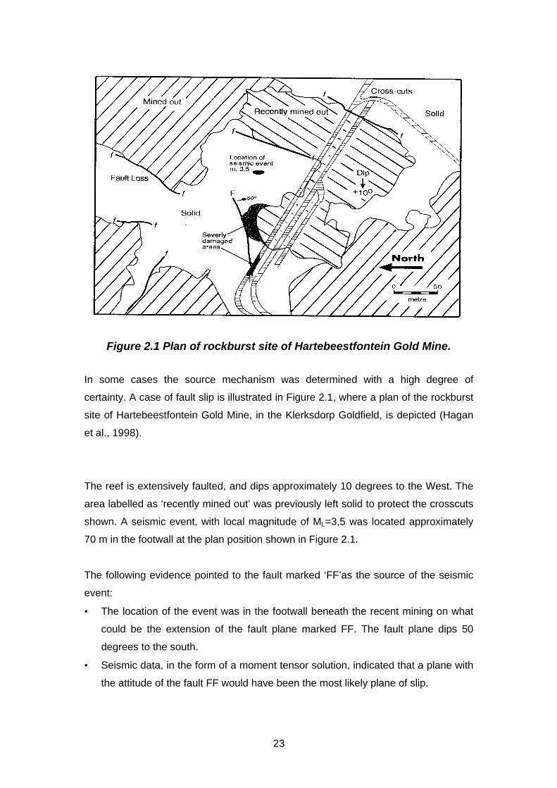
Figure 2.1 Plan of rockburst site of Hartebeestfontein Gold Mine.
In some cases the source mechanism was determined with a high degree of
certainty. A case of fault slip is illustrated in Figure 2.1, where a plan of the rockburst
site of Hartebeestfontein Gold Mine, in the Klerksdorp Goldfield, is depicted (Hagan
et al., 1998).
The reef is extensively faulted, and dips approximately 10 degrees to the West. The
area labelled as ‘recently mined out’ was previously left solid to protect the crosscuts
shown. A seismic event, with local magnitude of ML=3,5 was located approximately
70 m in the footwall at the plan position shown in Figure 2.1.
The following evidence pointed to the fault marked ‘FF’as the source of the seismic
event:
• The location of the event was in the footwall beneath the recent mining on what
could be the extension of the fault plane marked FF. The fault plane dips 50
degrees to the south.
• Seismic data, in the form of a moment tensor solution, indicated that a plane with
the attitude of the fault FF would have been the most likely plane of slip.
24
• Damage in the crosscut was most intense at the intersection of the fault with the
crosscut and took the form of fractured sidewall and footwall particularly on the
north side of the tunnel. The severity of the dynamic loading in this area was
evident when it was noticed that spare rails stacked on the north side of the
tunnel had been moved underneath the previously installed sleepers.
• Closure was most evident in the panel closest to the fault. Timber and composite
timber/brick packs were badly damaged.
• Rapid yielding hydraulic props had punched into the footwall indicating the
possibility of dynamic loading in excess of 3 m/s.
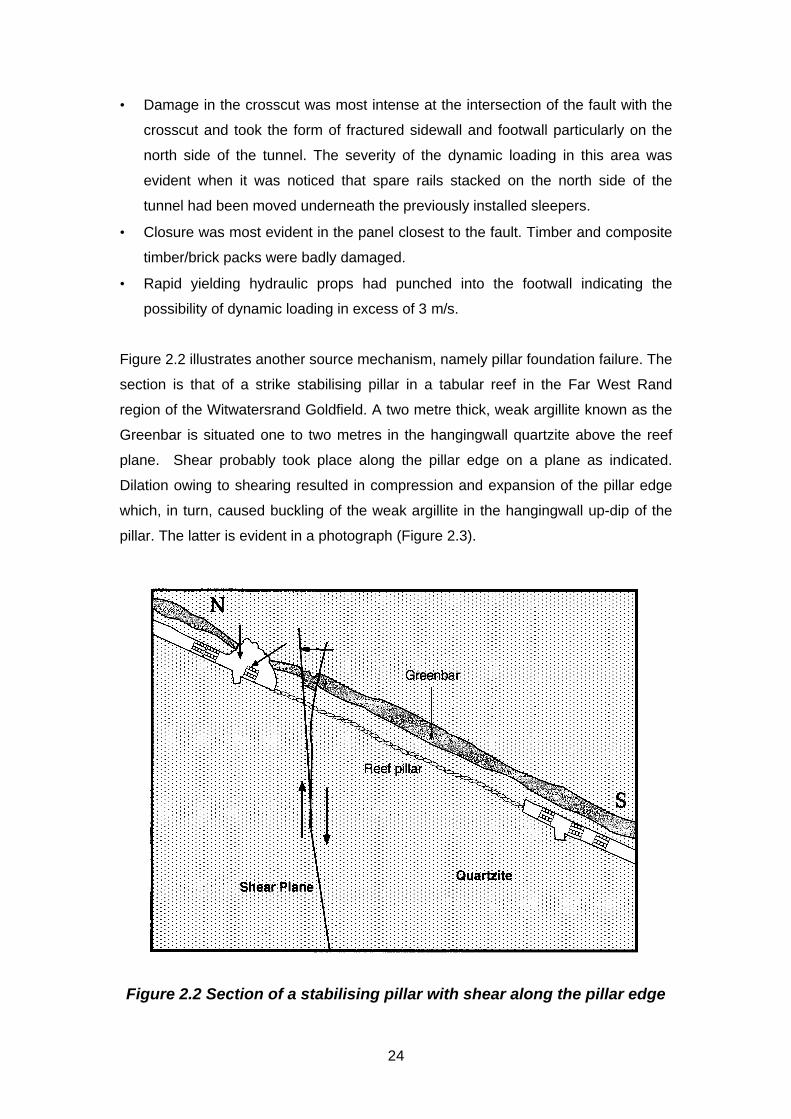
Figure 2.2 illustrates another source mechanism, namely pillar foundation failure. The
section is that of a strike stabilising pillar in a tabular reef in the Far West Rand
region of the Witwatersrand Goldfield. A two metre thick, weak argillite known as the
Greenbar is situated one to two metres in the hangingwall quartzite above the reef
plane. Shear probably took place along the pillar edge on a plane as indicated.
Dilation owing to shearing resulted in compression and expansion of the pillar edge
which, in turn, caused buckling of the weak argillite in the hangingwall up-dip of the
pillar. The latter is evident in a photograph (Figure 2.3).
Figure 2.2 Section of a stabilising pillar with shear along the pillar edge

25
Figure 2.3 Buckling of the Greenbar in the gully hangingwall.
The following evidence tends to support foundation failure as a source mechanism:
• Damage was detectable along 60 m of the gully on the north side of the pillar.
• Buckling of the Greenbar was clearly visible in sections of the hangingwall up-dip
of the pillar.
• The location of the main seismic event was in the footwall below the pillar.
• The moment tensor solution indicated that slip along this plane was the likely
source.
• Aftershocks were located approximately on the plane in the footwall below the
pillar.
2.3 Damage Mechanisms
The 34 investigations showed the most common damage mechanism to be collapse
and shakedown of hangingwall. Less common were tunnel wall damage, footwall
heave and face rock ejection.
26
Many factors affected the severity of damage. Mine layout factors included poor
remnant shape, deficient pillar design, breast mining on to geological features and
excessive leads or lags between panels. Incorrect input parameters such, as k-ratios
when modelling also resulted in inappropriate layouts for a stress field. Tunnels
positioned in fault loss zones sustained serious damage in some cases.
Inappropriate and poorly designed support in tunnels, gullies and stopes and in some
cases sub-standard application of the support in these excavations also played a role
in determining the severity of the sustained damage.
Certain rockburst investigations served to highlight problem areas that apply widely in
the industry. The areas are:
• A lack of knowledge of the stress fields affecting a particular mine.
• An underestimation of the extent of the unstable zone surrounding tunnels.
• Poor condition of tunnel support elements owing to corrosion.
• Siting of tunnels in zones of fault losses and tunnels intersecting faults at oblique
angles.
• Inappropriate gully support.
• Shape of remnant pillars.
• Backfill usage.
In September of 1997 a ML = 4,4 seismic event with two significant aftershocks
occurred in the vicinity of East Driefontein No. 4 sub-vertical shaft. Serious damage
was sustained in tunnels on four levels between 2400 m and 2800 m below surface.
The investigation served to illustrate that the in situ stress fields, in which the mining
excavations are created, significantly influence the type of stability problems that can
occur in an area.
Stress measurement work, subsequent to the above-mentioned activity, revealed
that an anomalous stress field exists where the horizontal stress component is
greater than that of the vertical. The seismic events mentioned above are now
thought to be associated with slip on two major geological features in the area.
Knowledge of such a stress field would assist significantly with mine design
(numerical modelling) both for local and regional support.

27
Stacey and Wesseloo (1998) have set up a database of stress measurements made
in Southern Africa over the past 30 to 40 years. Sponsored by SIMRAC the data are
available and should be used by the mining industry. From the point of view of
planning of mining operations, the in situ stress field is a most important input
parameter for modelling of excavations. As Stacey and Wesseloo (1998) rightly point
out, if the incorrect input values for the stresses are used, it is possible that the layout
or other modelling, and conclusions arising therefrom may be invalid. This may have
significant and adverse implications for stability and safety.
The data show that the horizontal stress orientations in the Klerksdorp area are
significantly different from those in the Far West Rand and Free State regions. The
data also show that the assumption of a k-ratio of 0,5 in the Far West Rand and
Klerksdorp regions is not valid in most cases. The ratio varies locally and there is
often a significant horizontal stress anisotropy that should not be ignored when
modelling mining sequences in such areas. Programs such as MINSIM_W can
accommodate the different horizontal stresses and thus provide, for example, more
realistic ESS values on fault planes. Unfortunately, the degree of spatial variations in
stress is poorly understood. There are therefore no well defined guidelines as to the
number of stress measurements necessary or to the correct means to estimate
stress when a limited number of measurements have been made.
In the investigation at East Driefontein serious damage was observed in tunnels and
crosscuts in the vicinity of the No. 4 sub-shaft. The damage was owing to failure of
the support system when subjected to dynamic loading associated with seismic
activity.
The degree of corrosion of the tunnel support, particularly in the vicinity of faults, was
high. Failure mechanisms, some of which are evident in a photograph (Figure 2.4),
included:
• bulking of the tunnel side- and hangingwall
• shearing and tensile failure of rebars
• pulling out of rebars
• corrosion and consequent failure of tendons and fabric support
• failure along weak joints

28
Figure 2.4 Various forms of support failure in a tunnel.
Where tunnels are needed for extended periods, and where seismic activity is likely,
it would be wise to identify areas where the support system has been compromised.
A systematic programme of pull tests coupled with basic observation of rock and
support conditions could achieve this.
The length and spacing of tendons depends on the depth of the unstable zone and
needs to be estimated. This can be done by means of petroscope observations and
extensometer monitoring thus giving the extent of fracturing and dilation of the tunnel
walls respectively. Extent of fallout in previous falls and rockbursts will also give
some idea of the depth of instability with which one is dealing.
Other recommendations made in this particular case were:
• shotcrete before meshing and lacing to avoid adhesion and variable thickness
problems
• consider injection of resin where ground conditions are exceptionally poor
• identify likely seismogenic structures from data available
The damage resulting from a local magnitude ML = 4,0 seismic event was
investigated in the vicinity of No. 5 Shaft at Vaal Reefs. The damage was restricted to

29
haulages, crosscuts and gullies on 60 and 62 levels some 1900 m below surface.
The Klerksdorp area is generally dominated by NE-SW striking faults, many of which
have been intruded by dykes. Large seismic events are in most cases associated
with these and with large bedding-parallel faults (Van den Heever, 1982). The
rockburst damage was found to be largely restricted to haulages and crosscuts within
a fault loss and was especially pronounced where the crosscuts intersected the fault
plane and passed from overstoped to solid ground. This investigation further
illustrated the need to more accurately gauge the depth of the unstable zone, which
increased significantly where the crosscuts intersected the fault plane. Either the
length of tendons should be increased and/or the spacing of tendons should be
decreased in such situations. This has the effect of increasing the interaction
between reinforcements to form a stable arch. Consideration should also be given to
the shear and yield capacity of the tendons for the anticipated design environment.
One of these major faults has a history of large (ML>3,9) seismic events. The
decision to site tunnels in the loss associated with this fault was made at the start of
mining. In retrospect it would appear that the siting of tunnels and crosscuts should
have been avoided in those fault loss areas where extensive stoping of nearby reef
was planned. Some knowledge of the stress regime and the presence of high
tectonic stresses in the vicinity of some of the faults would have been useful at the
early stages of planning. Slip on faults is uneven owing to variations in the type of
country rock and therefore residual anomalous stresses occur in the vicinity of the
fault. As a general rule tunnels should be kept away from faults and tunnels crossing
faults should not be highly stressed by mining.
In the course of this investigation it was also possible to compare the performance of
two types of gully support namely timber packs and cementitious packs on the gully
edges. The latter performed well and did not appear to induce additional damage to
the gully sidewalls while still providing adequate hangingwall support. The opposite
was true for many of the observed timber packs. The cementitious packs were
designed to yield at a load lower than that required to induce damage in the gully
sidewall. In addition the peak stress build-up under dynamic loading in the case of a
seismic event is significantly less (probably of the order of 30%) than that of a timber
pack.
A local magnitude ML=2,1 seismic event occurred approximately 2300 m below
surface at Deelkraal Gold Mine on the VCR horizon (Hagan et al.,1998). Evidence
30
listed below points to the failure of a remnant pillar as the most likely mechanism
(refer to Figure 2.6):
• Down-dip siding packs between points C and E had been pushed into the gully.
• Convergence, estimated at between 10 mm and 150 mm, was detected by
means of fresh splitting of timber on packs at points A, C, D and E.
• No recent movement was evident on the fault that was exposed at point B.
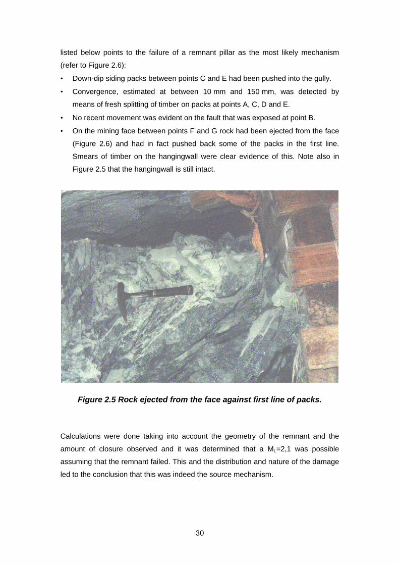
• On the mining face between points F and G rock had been ejected from the face
(Figure 2.6) and had in fact pushed back some of the packs in the first line.
Smears of timber on the hangingwall were clear evidence of this. Note also in
Figure 2.5 that the hangingwall is still intact.
Figure 2.5 Rock ejected from the face against first line of packs.
Calculations were done taking into account the geometry of the remnant and the
amount of closure observed and it was determined that a ML=2,1 was possible
assuming that the remnant failed. This and the distribution and nature of the damage
led to the conclusion that this was indeed the source mechanism.

31
Figure 2.6 Site of the remnant pillar on Deelkraal Gold Mine.
A pillar is in danger of crushing if it is reduced to a critically small width such that a
low width to height ratio leads to failure of even one limb of that pillar. In this case the
L-shape was poor. Also the trench, shown in Figure 2.6, to negotiate a 2 m roll
increased the effective height. The effective height may also have been increased by
the presence of weak hangingwall partings in the form of bedding-parallel faults.
A stoping layout giving rise to a triangular-shaped remnant would tend to fail at the
apices of the triangle leaving the core intact. In this case matters would have been
improved had underhand mining been done from the raise.
Further investigations have shown that similar mechanisms could be at work
elsewhere. An example is the investigation at Western Deep Levels South Mine
(Spottiswoode et al. 1998), where face bursting at 2400 m below surface generated a
ML=1,4 local magnitude seismic event. A highly stressed area, again on the VCR
horizon, was being mined at the time.
32
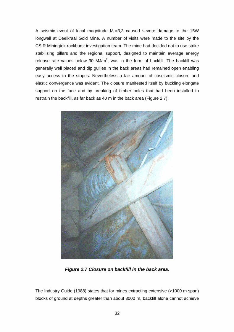
A seismic event of local magnitude ML=3,3 caused severe damage to the 15W
longwall at Deelkraal Gold Mine. A number of visits were made to the site by the
CSIR Miningtek rockburst investigation team. The mine had decided not to use strike
stabilising pillars and the regional support, designed to maintain average energy
release rate values below 30 MJ/m2, was in the form of backfill. The backfill was
generally well placed and dip gullies in the back areas had remained open enabling
easy access to the stopes. Nevertheless a fair amount of coseismic closure and
elastic convergence was evident. The closure manifested itself by buckling elongate
support on the face and by breaking of timber poles that had been installed to
restrain the backfill, as far back as 40 m in the back area (Figure 2.7).
Figure 2.7 Closure on backfill in the back area.
The Industry Guide (1988) states that for mines extracting extensive (>1000 m span)
blocks of ground at depths greater than about 3000 m, backfill alone cannot achieve
33
satisfactory regional support or ERR control. The Guide goes on to say that
theoretical studies indicate that hybrid systems of pillars and backfill combined can
offer significant advantages in terms of ERR reduction. In hindsight it would have
been better to have this combination at Deelkraal even though the depth of the 15W
longwall is not quite 3000 m below surface. Recent results from the Anglogold mines
on the Far West Rand show the hybrid systems to be effective in reducing the
seismic hazard (Essrich and Amidzic, 1999).
It can be shown numerically that such a hybrid system is more effective when the
stabilising pillars are orientated in a dip direction as in the case of the Sequential Grid
mining system practised at Elandsrand Gold Mine. In this case, unlike the longwall
system with strike oriented pillars, the backfill is placed into areas where far less
closure has been allowed to take place thus rendering the backfill more effective as
the span increases.
Arguments have been put forward, particularly for certain geotechnical area the Vaal
Reef in the Klerksdorp area, that backfill may not be effective as a local support
owing to the increased horizontal stresses that may result in an unstable stope
hangingwall beam. The validity of this argument needs to be substantiated with
documented evidence arising from underground observations and measurements.
SIMRAC sponsored research will be attending to this requirement in 1999.
An investigation of a rockburst site on West Driefontein Gold Mine showed the
positive effect backfill has on gully and stope conditions on the Carbon Leader Reef
horizon. Slip on a dyke contact caused a seismic event of local magnitude ML=2,7
that resulted in rockburst damage in four panels and gullies on a longwall 2300 m
below surface. The backfill at that time covered 67% of the mined-out area but was
unfortunately unevenly spread owing to operational problems. Only certain sections
of the upper panels were filled and it was very apparent that the gully opposite those
unfilled areas had suffered severe damage. The mechanism appeared to be
shakedown of the gully hangingwall after failure of the beam. The beam length
should be restricted as much as possible by bringing the backfill down close to the
gully. Cementitious gully packs with 1400 kN yield force were being used. This was
thought to be too strong and resulting in damage to the gully sidewall, particularly in
the areas opposite the non-filled zones in the stope. Some of the packs had in fact
fallen out completely. One of the recommendations was to use packs with a yield
load closer to 1000 kN.

34
2.4 Conclusions and Recommendations
1. The most common source mechanism of a causative seismic event is slip on
either a dyke contact or a fault. In some cases the seismic data coupled with the
extent, nature and location of the damage allow the identification of the source
mechanism with a high degree of confidence.
2. Other identified source mechanisms include remnant pillar failure, stabilising pillar
foundation failure and face bursting.
3. The most common damage mechanism resulting from seismic activity is
predictably, collapse and shakedown of hangingwall. Other mechanisms are
tunnel wall damage, footwall heave and face rock ejection.
4. Many factors affected the severity of damage and contributed to the occurrence
of violent seismic event. Mine layout factors included poor remnant shape, poor
pillar design, breast-on face orientation when approaching geological features
and excessive leads or lags between panels. Incorrect input parameters, such as
k-ratios, when modelling also resulted in poor layouts. Tunnels positioned in fault
loss zones sustained serious damage in some cases. Inappropriate and poorly
designed support in tunnels, gullies and stopes and in some cases sub-standard
application of the support in these excavations also played a role in determining
the severity of the damage sustained.
5. Assumptions regarding the stress field affecting a particular mine are probably
invalid in many cases. An improved knowledge of the stress field would assist
significantly with mine layout (numerical modelling) and both local and regional
support planning. It is recommended that mines make use of a database of stress
measurements that has recently been established additional stress
measurements may be necessary where anomalous situations are evident or
anticipated.
6. The degree of corrosion of tunnel support can have a significant effect on the
extent and severity of damage resulting from a seismic event. Where tunnels are
needed for extended periods, and where seismic activity is likely, areas where
support may be compromised must be identified and rehabilitated.

35
7. The depth of the unstable zone surrounding tunnels needs to be estimated. This
determines the necessary/optimal length and spacing of tendon support.
8. The siting of tunnels and crosscuts in fault loss zones where extensive mining of
nearby reef is planned should be avoided.
9. Cementitious packs, designed to yield at loads lower than that required to induce
damage in the gully sidewall, have been seen to perform well under dynamic
loading. In one case this was confirmed by a direct comparison with timber
packs.
10. The stability of remnant pillars depends largely on the shape and the width:
height ratio. The latter may be affected by local geology and by reef geometry. A
triangular shape as opposed to L-shaped or narrow rectangular remnants, which
are particularly troublesome, is recommended.
11. Backfill can be shown to have a significant regional and local support benefit in
some areas particularly on the Far West Rand. The positive effect that backfill
has on gully and stope conditions has been observed.
3 Controlled seismic source experiment
3.1 Introduction
Rockbursts are a major hazard in South African deep-level gold mines. Many
analyses have been made and many observations of rockburst damage have been
carred out. Despite these efforts, the rockburst problem is far from solved.
An artificial rockburst experiment was conducted as a part of this project with the
collaboration of GAP 335. An attempt was made to simulate a seismic event by
means of a large blast in solid rock close to a crosscut. The idea was to instrument
the resultant “rockburst” site in order to gain further insight into the damage
mechanisms involved. An experiment site was set up in a disused crosscut on 53
36
level (1600 m below surface) on Kopanang Mine previously called Vaal Reefs No. 9
Shaft. The experiment involved a designed source, a fairly dense array of seismic
monitoring, extensometer measurements, petroscope observations and study of rock
mass condition (fractures, joints, rock strength etc.). Knowledge of the site before
and after the experiment was gained using ground penetration radar and seismic
measurements.
Earlier attempts at this experiment were unsuccessful and success was only
achieved in the middle of September 1998, three months before the end of this
project. The quantity and quality of the data exceeded our initial expectations, and
more time was required to complete these analyses. The following document is
therefore incomplete and it is hoped that further opportunity will arise for a more
detailed analysis.
3.2 Test site and instrumentation
The site is situated at Kopanang mine (9 shaft), Vaal River Operations at the 53
BW23 X/C South. The crosscut is 2118 m below datum or 1600 m below surface.
The lithologies in the crosscut comprise argillaceous quartzites of the Strathmore
Formation known locally as the MB2. The quartzites are grey, medium grained and
argillaceous. The bases of individual beds are coarser, defining an upward fining
sequence. Each bed is usually capped by a dark green argillite up to 5 mm thick.
Bedding is generally planar with thicknesses ranging from 50 mm – 500 mm. Black
argillite lenses occur locally within the quartzites and are laterally impersistent.
A N-S trending normal fault dipping 720 to the east occurs 10 m NW from the site.
The fault has a throw of over 100 m downthrow to the east. The lithology
encountered in the crosscut is thus hangingwall strata of the Vaal Reef. There is
some evidence of strike slip movement on the fault.
The site was located in an unused crosscut that was intersected by a crosscut. Five
blast holes were drilled from the crosscut in a direction parallel to the crosscut. The
charged portion of the holes was about 6 m from the tunnel sidewall. The holes were
drilled in a vertical plane with the collars about 500 mm apart. The purpose of this

37
design was to exclude gas expansion as a direct source of rock ejection. Figure 3.1
illustrates the underground layout and deployment of seismic sensors.
Main Blast261 Kg ANFO
Uniaxial accelerometer, HW-in solid
Uniaxial accelerometer, SW-surface
Uniaxial geophone, SW-surface
Uniaxial geophone, HW-surface
Uniaxial geophone, FW-surface Triaxial geophone, SW-surface
Triaxial geophone, SW- in solid
Calibration blast
Area of damage
HID LID
HID - high intensity damageLID - low intensity damage
C
B
A
A, B & C - ground motion monitor site
Figure 3.1 Controlled seismic source experiment layout and deploymentof the seismic sensors.
Three accelerometers PCB 305A04, shock type, were installed close to the
projection of the blast on the tunnel wall. Two of them were placed on the sidewall
closest to the blast in the area of maximum expected damage and the third one was
installed in a nearby borehole 3 m deep into the hangingwall.
The output from the accelerometers was conditioned using in-line amplifiers set at
1 x times gain. A Speedwave, 4 channel, high-speed digital recorder was used to
record the signals. The recorder has a 12 bit resolution and was set at a voltage
range of ± 10 V and a sample rate of 500 000 samples per second.
Three 8 channel ground motion monitors were installed along the tunnel at the both
sidewalls, the hangingwall and the footwall. Vertical, horizontal and triaxial boats,
installed on the skin and into a borehole were used to supply maximum seismic
coverage. see Figure 3.1.
Additional measurements of tunnel deformation before and after the experiment were
done using extensometers, ground penetration radar and routine geological
38
techniques such as fracture mapping, assessment of the existing faults and joints
and petroscopic observations. Rock ejection velocities during the blast were filmed
using a high-speed video camera.
3.3 Calibration blast and pre-blast monitoring
Preliminary modelling and the use of empirical equations for calculation of peak
particle velocities gave large variations in expected peak particle velocities. It was
therefore decided to perform a small calibration blast.
The blast was conducted into the blasting wall close to the last set of geophones (see
Figure 3.1). A horizontal hole, 0,37 mm in diameter drilled 750 towards the end of the
tunnel was charged with five cartridges Powergell 816 with 0,12 kg each equivalent
to 0,66 kg ANFO. The 0,65 m length charge was stemmed with 1,15 m clay. The
estimated Velocity of Detonation (VOD) was 4500 m/s.
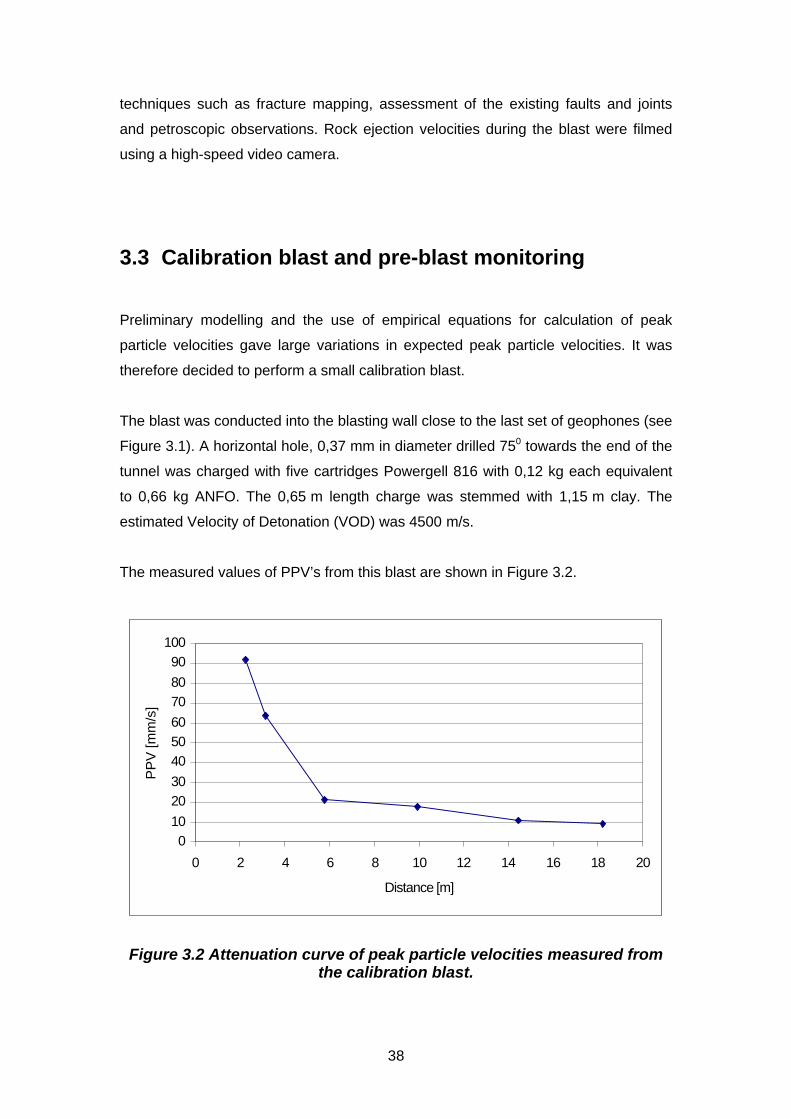
The measured values of PPV’s from this blast are shown in Figure 3.2.
010
2030
405060
7080
90100
0 2 4 6 8 10 12 14 16 18 20
Distance [m]
PP
V [m
m/s
]
Figure 3.2 Attenuation curve of peak particle velocities measured fromthe calibration blast.

39
The attenuation of maximum velocities for the calibration blast Y(R) as a function of
distance R was derived as:
1.1
1')(R
CRY = (3.1)
where: C” is a constant proportional to the charge mass.
It was important to estimate the parameters of the main blast and predict the position
and the value of maximum velocities on the blasting wall. The charge mass of the
calibration blast, Powergell 816, was converted to the equivalent mass ANFO, using
1,1 convergent coefficient. Then the peak particle velocity was estimated as a
function of the charge mass Q and the distance R. The following equations have
been suggested by Rorke (1998), for far field:
PPV = 1143(R/(Q^0,5)^-1,6 (3.2)
where: R is a distance in m and Q = Charge mass in kg
Another equation for far field measurements was given by Ouchterlony et al, (1997):
PPV = 650(R/(Q^0,5)^-1,42 (3.3)
Persson and Holmberg, (1990) have scaled the equation (3.2) for the near field using
a scaling factor f = [atan(H/2R)/(H/2R)], where and H is a charge length in m:
PPV = 650(R/(fQ^0,5)^-1,42 (3.4)
The maximum velocities in respect of the number of holes and the charge mass for
5 m long holes were calculated using Equations (3.2), (3.3) and (3.4) and the results
are listed in Table 3.1

40
Table 3.1
Maximum velocities as a function of charge mass and numbers of holes,according to the Equations 3.1, 3.2, and 3.3.
Charge Mass Rorke
Far Field
Ouchterlony
Far Field
Persson & Holmberg
Near Field
1 Hole 40 1664,72 907,48 861,91
2 Holes 80 2898,45 1484,46 1409,91
3 Holes 120 4009,03 1979,68 1880,26
4 Holes 160 5046,50 2428,29 2306,34
5 Holes 200 6032,79 2845,16 2702,28
However, these equations are empirically obtained and are based on site-specific
measurements. For more accurate estimation of the maximum velocities numerical
modelling was needed.
3.4 Numerical modelling for planning the main blast
and expected velocities
A more detailed coverage of numerical modelling of this experiment is given in the
GAP 332 final report (Napier et al., 1998). Numerical modelling was used both in a
forward sense in the design phase, as well as for back analysis to develop an
understanding of wave interaction with tunnels.
Source Model
A numerical source was required which would model stress waves emanating from a
propagating blast in a borehole, to a distance many times larger than the borehole
radius. (In the experiment, the borehole charge lengths were from 4 to 7 m and the
borehole diameter was 0,1 m. The tunnel was more than 5 m away, and geophones
were located up to 25 m ahead of the blast). A three-dimensional numerical model
with this volume of interest required as coarse as possible a representation of the

41
source to be developed. i.e. it would be pointless to model the borehole in any detail,
and ideally the source diameter should require just a single element.
The assumed model was one of a moving radial load applied to the surface of a
borehole, where the position of the applied load moves along the axis of the borehole
with a certain velocity of detonation (VOD). Through comparisons with an analytic
solution for this source model (Kouzniak, 1998; Kouzniak & Rossmanith, 1998), it
was found that the source could be represented numerically as a volumetric source
without the explicit representation of a borehole, and coarsely, with a single element
width corresponding to the borehole diameter. Comparisons made showed that the
coarse numerical source corresponds accurately with the analytic source. It was also
observed that this source generates shear waves owing to the non-uniform loading of
the borehole surface, and that for VOD < Cp, the shear wave is dominant (Napier et
al, 1998).
Forward modelling of the experiment using this source model
An approximate representation of the tunnel experiment was made in the program
WAVE (Hildyard et al, 1995). A true 3D cavity was not available to simulate the
tunnel, and an approximation was made - the free surface conditions of the different
tunnel faces were modelled accurately, while the corners of the tunnel were poorly
represented. Forward numerical modelling was used to aid in the design of the
experiment, to give insight into which measurements were likely to be the most
useful, and insight into the positions where recordings should be made. The following
questions were identified:
• Can the experiment be tailored to simulate waves from a mining-induced
seismic event?
• Where is the expected position of maximum damage?
• How quickly do the motions die off with distance along the tunnel?
• How much damage can be expected on the other walls of the tunnel?
The maximum particle velocity on the tunnel sidewall was found to depend on the
following:
• The maximum borehole pressure: This is the assumed maximum pressure
reached at the walls of the borehole. The maximum velocity in the models is
linearly related to this pressure.

42
• The rise-time of the pressure: This is the duration over which a point on the
borehole wall moves from zero load to maximum load. The faster the rise time,
the higher the resulting velocities. This also determines the dominant frequency
of the incident waves.
• Delay between (the five) multiple blasts: The initial blast design anticipated a
delay of at least 1 ms between blasts (to allow for detonation error). The
modelling showed that this was too great a delay for the blasts to behave as a
single event i.e. velocities at the tunnel were greatly reduced if the individual
holes were detonated with large delays.
No definitive reference to aid in choosing these parameters could be found, but
based on blast modelling experience, the following values were assumed to be good
estimates (Daehnke, 1998). An upper maximum for the borehole pressure of 1 GPa,
and an upper maximum for the rise-time of pressure at a point of 200 µs. The latter
corresponds to maximum pressure reached over approximately 12 borehole radii.
Pressure decay time is much longer than the rise-time and its influence on wave
motions at the tunnel is negligible. Finally, the detonation method for the blast was
changed to give approximately simultaneous ignition.
The preliminary modelling demonstrated that:
• Predominantly shear waves could be generated by a suitable choice of VOD.
• The position of maximum damage depends on the VOD/Cs ratio of the blast
(where Cs is S-wave velocity), and the distance between the blast and the tunnel
wall.
• The magnitude of the maximum velocity (at the tunnel wall) depends on the
maximum borehole pressure, rise time of pressure at a point and time delay
between individual blasts. Estimates of velocity magnitudes at the tunnel would
be entirely dependent on meaningful estimates of these parameters.
• Estimates of motions on the other walls of the tunnel were considered unreliable,
since there was not a continuous tunnel free surface in this model, with spurious
stresses transmitted through the corners.

43
Calibration
It was important to estimate parameters such as the pressure and rise-time for the
source model, and indeed to evaluate whether this source model would be valid as a
representation of the blast. Accelerograms recorded very close to a blast in solid rock
were available from an earlier experiment (Rorke, 1992), obtained as part of the
preconditioning research project (Lightfoot et al, 1996) research project. Attempts to
model these with the chosen source model were not conclusive, and velocities in
models using the suggested blast parameter estimates were an order of magnitude
less than the recorded velocities. Greater detail is presented in GAP 332 (Napier et
al, 1998); but it became apparent that a calibration blast at the actual rockburst
experimental site providing velocities at greater distances from the blast, needed to
be made. Other data was available to calibrate the model in terms of empirical
expressions for far-field velocities due to a blast. Table 3.2 shows the source
parameters which were inferred from these calibrations, and used in different models
of the tunnel experiment. Other factors which affect the model results are the material
parameters. Values of Cp = 5740 m/s and Cs = 3514 m/s were used in all models,
based on estimates for solid rock at the site.
Table 3.2
Source parameters used to model the blast in the tunnel experiment.Initial estimates of these parameters did not match calibration data, from
which other parameters were derived.
Source #1,
from realistic
estimates
(Daehnke,
1998)
Source #2,
from
preconditioning
experiment
Source #3,
from
calibration
blast
Source #4,
used in post-
blast model
Maximum
borehole pressure
≤ 1 GPa 10 Gpa 9 GPa 1 Gpa
Pressure rise-time ≤ 200 µs 100 µs 800 µs 800 µs
Borehole diameter 0,1 m 0,2 m 0,3 m 0,2 m
VOD 4200 m/s 4200 m/s 4000 m/s

44
As mentioned above, a calibration blast was set off at the site. The physical
parameters, as given in Chapter 2, were: a 750 charge hole, 1 m from the tunnel wall,
0,65 m in length, 0,37 m in diameter and 0,66 kg in equivalent mass with a VOD of
4500m/s. The best modelling match was found with a source rise-time of 0,8 ms, a
diameter of 0,1 m (3 times the physical diameter), and a peak pressure of 9 GPa.
The long rise time seems necessary because of surprisingly long pulse widths in the
data - this differs significantly from data from the preconditioning experiment, where
pulse widths are much shorter. Two explanations are possible. The preconditioning
experiment measured motions very close to the blast, and the high frequencies
measured in the preconditioning experiments may attenuate rapidly to smaller values
at the distances associated with the calibration blast. Secondly, the geophones had a
filter at 800 Hz so that higher frequencies were not recorded for the calibration blast.
Comparisons for various geophones along the near tunnel wall are shown in
Figure 3.3. Geophones C8, C3, C6 and C5 are normal to the tunnel wall starting at
5,8 m from the calibration blast, and positioned at approximately 4 m intervals.

45
Geophone C8 Geophone C3
Geophone C6 Geophone C5
-0.4
Time(ms)
20.2
-20
-0.4
Time(ms) 20.2
-20
(i) Model
(ii) Observed
-0.4
Time(ms)
20.2
-8.5
20
Vel.(mm/s)
20
Vel.(mm/s)
8.5
Vel.(mm/s)
8.5
Vel.(mm/s)
-0.4
Time(ms)
20.2
-8.5
(i) Model
(ii) Observed
25
Vel.(mm/s)
-0.4
Time(ms)
20.2
-25
-0.4
Time(ms) 20.2
-25
(i) Model
(ii) Observed
-0.4
Time(ms)
20.2
-13
25
Vel.(mm/s)
13
Vel.(mm/s)
13
Vel.(mm/s)
-0.4
Time(ms) 20.2
-13
(i) Model
(ii) Observed
Figure 3.3 Comparison of model with geophone recordings fromcalibration blast, for modelled source of 9 GPa, 800 µµs rise-time, step
shape load and 0,1m diameter. Geophones C8, C3, C6 and C5 extendedin a line along the near tunnel wall, starting at 5,8 m from the blast and
in approximately 4 m intervals. Motion is normal to the tunnel wall.
Pre-blast Modelling
Although neither was ideal, two distinctly different source models were suggested
from the different calibration methods. These source models were applied in a model
of the final blast design before the actual blast, and later compared with the actual
blast.

46
From the calibration blast, the source for models of the main blast (source #3) was
inferred as:
- 0,8 ms rise time. (The rise-time cannot be directly inferred from the pulse width
of the measured waveforms, as the VOD has an influence as well).
- Diameter = 0,3 m. (3 times that of the real source)
- Peak Pressure = 9 GPa.
This produced more realistic maximum tunnel velocities (3 m/s from a single 8 m
blast hole) than the source derived from the preconditioning experiment (source #2).
A surprising result was that the position of maximum velocity was no longer ahead of
the blast (Figure 3.4), whereas in the earlier modelling the maximum was ahead of
the blast and strongly dependent on the VOD. This was found to result from the long
rise-time of the source. Although based on the calibration data, it was a much slower
rise-time than what was initially thought to be realistic. If the rise-time is reduced, the
maximum tunnel velocity shifts ahead of the blast again.
Variations of blast hole length and blast synchronisation were considered prior to the
blast. A 5 m blast hole produced a maximum tunnel velocity of 2,3 m/s compared to 3
m/s for the 8 m blast hole. Five synchronous blasts produced tunnel velocities more
than five times that of a single blast. Five asynchronous blasts, each with a 0,5 ms
delay, produced a maximum tunnel velocity of 7 m/s.
0.90.33.0m/s1.82.4
Blast-hole
Figure 3.4 Maximum velocity on tunnel wall for pre-blast model,source # 3 9 GPa, 800 µ800 µs, step shape load and 0,3 m diameter, with a
single 8 m blasthole.

47
Waveforms from this pre-blast model are compared with waveforms from the final
blast in Figure 3.5, for geophone positions at approximately 4 m intervals along the
tunnel wall. Experimental waveforms begin before the blast, so these have been
shifted into approximately the same time window as the model. In the case of the
experiment the maximum occurs in the initial P-wave pulse and there is virtually no
S-wave, while for the model the maximum occurs later due to arrival of the shear
wave. The maximum amplitudes are similar which indicates that the blast pressure is
too high in the source model, since the model was for a single blast hole.
(a) Velocity recordings (m/s) from final blast (b) Velocities (m/s) from pre-blast model, source #3
-4.9e-1
4.9e-1
0(ms) 26
-5.5e-1
5.5e-1
0(ms) 26
-9.5e-1
9.5e-1
0(ms) 26
-5.6e-1
5.6e-1
0(ms) 26
-7.9e-1
7.9e-1
0(ms) 26
-7.7e-1
7.7e-1
0(ms) 26
-8.2e-1
8.2e-1
0(ms) 26
-3.1e-1
3.1e-1
0(ms) 26
Vel.(m/s)
Time (ms)
C6
C4
C8
C5
Vel.(m/s)
Time (ms)
C6
C4
C8
C5
Figure 3.5 Comparison of the pre-blast model velocities for source #3with the final blast measurements for geophones C5, C6, C4 and C8starting at 7 m ahead of the blast, and at approximately 4 m intervals
along the tunnel wall.
Post-blast Modelling
A large amount of data has been gathered from the experiment and has been
partially analysed. Most of this has still to be considered from a modelling back-
analysis perspective. The validity of the source model has not been established,
since the predicted large shear wave is not present in the near field. A well-
developed shear wave was observed in the far field at 850 m from the source Figure
3 13 (a, b and c). Nevertheless, a model was run using the final blast positions, sizes,
synchronisation and recordings at all geophone positions. The borehole source was
reduced to 0,2 m diameter (two times the real diameter), and the pressure to 1 GPa,
with a 0,8 ms rise time. The correct lengths and positions of the five blast holes in the

48
final blast were represented in this model, and the modelled velocity profile along the
tunnel near wall is shown in Figure 3.6. It is encouraging that velocities approaching
the recorded values were obtained without the extremely high borehole pressures
suggested by the calibration modelling. However, once again it was found that the
shear component in the model was much greater than the P-wave component, which
was not the case in the experimental recordings. One possible explanation is the
complexity of the seismic signal in the near field. Both wave groups, compressional
and shear, arrived at the receiver at approximately at the same time and interfere
with each other. The separation of these phases is often impossible (Aki and
Richards, 1980).
Figure 3.6 Maximum velocities at near tunnel wall for the post-blastmodel source #4. Maximum velocity for a blast pressure of 1 GPa is
much lower than that recorded. Position of maximum velocity is nowopposite the blast holes, due to the relatively long wavelength, and
synchronisation of the blasts.
Conclusions
Encouraging results were obtained in the development of an equivalent source
representation to a set of blast holes. ‘Realistic’ parameters for rise-time, borehole
radius and borehole pressure produce velocities, which are much lower than
velocities from available data. Nevertheless altering the source produced some
encouraging waveform correspondence with the calibration data. The back-analysis
of the main experiment is still in progress.

49
The lack of a strong shear wave in the measurements of the final blast may indicate
that the source model is not valid. Two aspects are being investigated to produce
waves, which better correspond to the experiment. Work on a true tunnel cavity
implementation (in case spurious waves are due to the approximate numerical
implementation), and alteration of the source model or parameters which may reduce
the S-wave and increase the P-wave content.
One of the anticipated advantages of modelling data from a controlled experiment is
a detailed knowledge of the source so that source uncertainty is decoupled from the
investigation, allowing focus on the interaction with the excavation surface. So far this
goal has not been realised. An accurate source model needs to be developed for the
modelling phase to be useful, possibly requiring further experiments measuring
waveforms from blasts in solid rock.
3.4 Main blast
3.5.1 Source description
The purpose of this blast was to simulate a rockburst in a tunnel using explosive
energy as a source. However, one fundamental difference between a blast source
and dislocation type of rockburst is the effect of gas expansion. To prevent direct gas
expansion causing ejection, the experimental site was chosen in a crosscut that was
intersected by a crosscut. Five blast holes were drilled from the crosscut in a
direction parallel to the crosscut. They were about 6 m from the tunnel sidewall over
the charged portion of the holes. The holes were drilled in a vertical plane with the
collars about 500 mm apart. The exact position of the holes was surveyed relative to
the tunnel sidewall.
The holes were charged with 261,5 kg low density ANFO, using a compressed air
loader. The explosive distribution for each hole is given in Table 3.3. The holes were
stemmed with quick setting cement cartridges. The holes were initiated using 10 g/m
detonating cord with two Powergell 816 cartridges acting as boosters. The booster
position was located 1 m into the charge from the stemming end of the charge.
Table 3.3 provides a detailed charging report based on hole length (Rorke, 1998).

50
Table 3.3
Explosive Charging Details and Estimated Energies.
Hole 1 Hole 2 Hole 3 Hole 4 Hole 5
Explosive type ANFO ANFO ANFO ANFO ANFO
Charge Mass/Metre (kg/m) 8,60 8,60 8,60 9,01 9,01
Estimated in-hole density (g/cm3) 1,05 1,05 1,05 1,10 1,10
Length of stemming (m) 4,80 8,10 3,42 7,30 6,95
Hole Depth (m) 12,30 14,45 13,34 14,45 11,17
Hole Diameter (mm) 102 102 102 102 102
Explosive Mass Per Hole (kg) 49,89 54,62 54,53 64,43 38,03
Estimated explosive VOD (m/s) 3600 3600 3600 3800 3800
Estimated Energy (MJ Per Hole) 126,92 138,96 138,74 163,91 96,74
Estimated Borehole Pressure (Gpa) 2,90 2,90 2,90 3,20 3,20
Assuming that there were equal lengths of detonating cord down the barrel of each
hole, the hole firing times have been calculated and are listed below. The first hole to
fire was the bottom hole. The timing calculation is based on the tie-up of the cord
between holes. The cord length was 0,5 m between holes and the detonation velocity
of the cord was 7000 m/s. The firing times are given in Table 3.4.
Table 3.4
Firing times.Hole 1 284 microseconds
Hole 2 213 microseconds
Hole 3 142 microseconds
Hole 4 71 microseconds
Hole 5 0 microseconds
A graphical illustration of this explosive source including length of charge, length of
stemming, point of ignition and detonation times is given in Figure 3.7.

51
6.95
7.3
3.42
8.1
4.8
4.22
7.15
6.33
6.35
5.8
3.62
1.7
0 1 2 3 4 5 6 7 8 9 10 11 12 13 14 15
Hole length [m]
Stem
Charge
Air Gap
Hole # 471 µs
Hole # 3142 µs
Hole # 2213 µs
Hole # 1284 µs
Hole # 50 µs
Direction of ignition
Figure 3.7 Graphical illustration of the main blast source.
3.5.2 Seismic observations in the near field
Ground velocities as measured by the accelerometers in the area of damage
Three accelerometers were installed in close proximity to the blast. Two were placed
on the sidewall, close to the blast, in the area of maximum expected damage. The
third was installed in a borehole 3 m in the hangingwall, to supply a measure of the
waves in solid rock (see Figure 3.1). This accelerometer was also used as a
reference for comparison of maximum velocities recorded in solid rock and on the
skin of the tunnel.
The accelerograms recorded in this area are plotted in Figure 3.8 (a, b, and c).

52
-100000
-80000
-60000
-40000
-20000
0
20000
40000
60000
80000
100000
12 13 14 15 16 17 18 19
ms
m/s
^2
Figure 3.8 (a) The accelerogram recorded in the area of high-intensitydamage. This accelerometer was ejected at 3.3 m/s.
-100000
-80000
-60000
-40000
-20000
0
20000
40000
60000
80000
100000
12 13 14 15 16 17 18 19
ms
m/s
^2
Figure 3.8 (b) The accelerogram recorded in the area of low-intensitydamage.

53
-100000
-80000
-60000
-40000
-20000
0
20000
40000
60000
80000
100000
12 13 14 15 16 17 18 19
ms
m/s
^2
Figure 3.8 (c) The accelerogram recorded in the solid rock 3 m into thehangingwall close to the area of damage.
As the accelerograms developed a DC off-set it was necessary to perform a high-
pass filter before the integration to velocity.
The accelerograms a(t) were integrated in order to obtain the ground velocities v(t)
according to the following equation:
∫= 2
1
)()(t
tdttatv (3.5)
Numerically the integration was performed as:
ttftvtv iit δ)()()( 1 += − (3.6)
where: a(t) is the time history of acceleration, f(t) is a high-pass filter and v(t) is the
time history of velocity
The peak velocities obtained from accelerometers ACT, ACM and ACH are given in
Table 3.5.

54
Table 3.5
Velocities obtained from the blasting.
Accelerometer Particle
Velocity [mm/s]
Remarks
ACT 3328 Located in the area of high intensity damage
(HID): ejected
ACM 1626 Located in the area of low intensity damage
(LID): not ejected
ACH 1175 Located in the solid rock, 3 m into the
hangingwall: not ejected
Ejection velocities from high speed video camera
A “Locam” high-speed camera was used to film the tunnel sidewall to measure rock
fragment displacement. The camera is capable of filming at a rate of 500 frames per
second. However, lighting conditions in the tunnel were not sufficient, and the frame
rate had to be reduced to 200 frames per second. This frame rate provided a time
resolution of 5 ms per frame.
Nine 100 mm orange coloured balls were positioned on the tunnel wall closest to the
charges. They were located 1 m apart vertically and 2,5 m apart horizontally. The
purpose of the balls was to provide locality information and scaling from the high-
speed film.
The balls were positioned in three vertical sets of three. The first vertical set was
located directly opposite the centre of the explosive charges. The second set was
located in the toe vicinity of the charges and the third set was located 2,5 m farther
away.
Due to the insufficient lighting, only the top two balls of the third vertical set could be
seen. Displacement recordings given in the following section therefore relate to a
position that is 2,5 m east of the hole bottoms.

55
The data from the high-speed camera was hampered by poor lighting conditions.
Therefore fragment velocities could only be measured in the top eastern segment of
the monitored zone.
The conventional film was converted into VHS video tape and “BMP” computer files.
Fragment velocities were measured by tracking individual fragment positions through
space at intervals of 10 frames (equal to 50 ms). This was done manually by
measuring displacements on the projected image and converting these to actual
distances using the target ball positions for scaling. Table 3.6 provides the original
measurement information and the conversion to displacement using a correction for
the angle of the camera to the axis of the tunnel.
The equation used to convert from the projected image displacement distances to
actual displacement distances was:
Displacement = (Projected image displacement x 8,457)/cos (140) (3.7)
The factor 8,457 converts from image pixels to actual distances in mm and was
obtained by measuring the projected image distance between two marker balls. The
angle of the camera to the north wall of the crosscut was 140. The correction factor
cos(140) was applied because it is assumed the rock fragments were ejected at right
angles to the tunnel wall.

56
Table 3.6
Measurements of displacement from 7 fragments, clearly visible on theframe.
Frame Time (ms) Dist (mm) Velocity (m/s)
Ball
0 0 0,00 0,00
10 50 57,27 1,15
20 100 105,74 2,11
25 125 96,92 3,88
30 150 88,11 3,52
35 175 185,04 7,40
Fragment 2
0 0 0,00 0,00
10 50 42,29 0,85
20 100 0,00 0,00
25 125 0,00 0,00
30 150 0,00 0,00
35 175 0,00 0,00
Fragment 3
0 0 0,00 0,00
10 50 35,25 0,70
20 100 70,49 1,41
25 125 39,65 1,59
30 150 0,00 0,00
35 175 0,00 0,00
Fragment 4
0 0 0,00 0,00
10 50 30,84 0,62
20 100 66,09 1,32
25 125 123,36 4,93
30 150 0,00 0,00
35 175 0,00 0,00
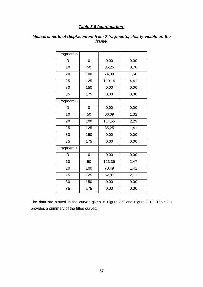
57
Table 3.6 (continuation)
Measurements of displacement from 7 fragments, clearly visible on theframe.
Fragment 5
0 0 0,00 0,00
10 50 35,25 0,70
20 100 74,90 1,50
25 125 110,14 4,41
30 150 0,00 0,00
35 175 0,00 0,00
Fragment 6
0 0 0,00 0,00
10 50 66,09 1,32
20 100 114,55 2,29
25 125 35,25 1,41
30 150 0,00 0,00
35 175 0,00 0,00
Fragment 7
0 0 0,00 0,00
10 50 123.36 2,47
20 100 70,49 1,41
25 125 52,87 2,11
30 150 0,00 0,00
35 175 0,00 0,00
The data are plotted in the curves given in Figure 3.9 and Figure 3.10. Table 3.7
provides a summary of the fitted curves.

58
Displacement Curves
0.00
20.00
40.00
60.00
80.00
100.00
120.00
140.00
160.00
180.00
200.00
0 50 100 150 200
Time (ms)
Dis
plac
emen
t (m
m) Ball
Fragment 2Fragment 3Fragment 4Fragment 5Fragment 6Fragment 7
Figure 3.9 Displacement curves for six fragments and one marker ball.
It can be seen from Figure 3.9 for time later than 100 ms the measurements become
random, perhaps due to the interaction of the camera with the anther particles or with
incoming air wave. In Figure 3.10 all points above 100 ms has been excluded.
Displacement Curves
0.00
50.00
100.00
150.00
200.00
250.00
300.00
350.00
400.00
450.00
500.00
0 50 100 150 200
Time (ms)
Dis
plac
emen
t (m
m)
Ball
Fragment 2
Fragment 3
Fragment 4
Fragment 5
Fragment 6
Fragment 7
Linear (Ball)
Linear (Fragment 2)
Linear (Fragment 3)
Linear (Fragment 4)
Linear (Fragment 6)
Linear (Fragment 5)
Linear (Fragment 7)
Figure 3.10 Fitted curves limited to first 100 ms of data. The secondpoint for fragment 7 has been omitted.
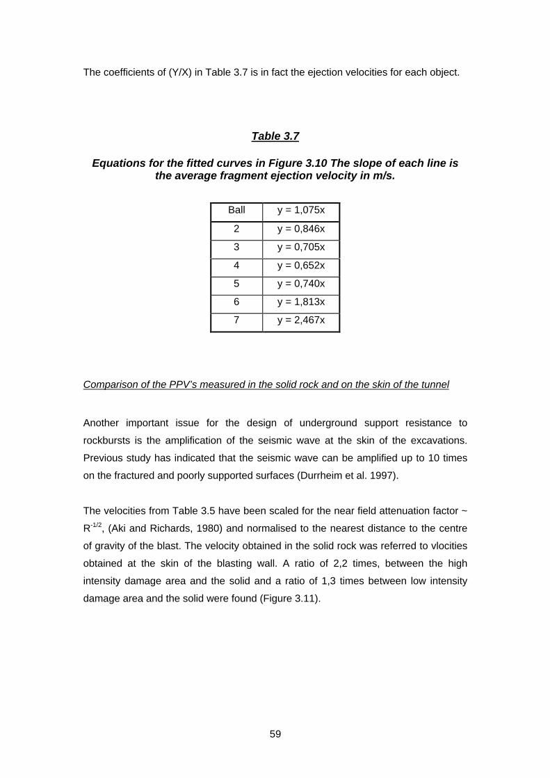
59
The coefficients of (Y/X) in Table 3.7 is in fact the ejection velocities for each object.
Table 3.7
Equations for the fitted curves in Figure 3.10 The slope of each line isthe average fragment ejection velocity in m/s.
Ball y = 1,075x
2 y = 0,846x
3 y = 0,705x
4 y = 0,652x
5 y = 0,740x
6 y = 1,813x
7 y = 2,467x
Comparison of the PPV’s measured in the solid rock and on the skin of the tunnel
Another important issue for the design of underground support resistance to
rockbursts is the amplification of the seismic wave at the skin of the excavations.
Previous study has indicated that the seismic wave can be amplified up to 10 times
on the fractured and poorly supported surfaces (Durrheim et al. 1997).
The velocities from Table 3.5 have been scaled for the near field attenuation factor ~
R-1/2, (Aki and Richards, 1980) and normalised to the nearest distance to the centre
of gravity of the blast. The velocity obtained in the solid rock was referred to vlocities
obtained at the skin of the blasting wall. A ratio of 2,2 times, between the high
intensity damage area and the solid and a ratio of 1,3 times between low intensity
damage area and the solid were found (Figure 3.11).

60
0
500
1000
1500
2000
2500
3000
3500
Distance from the blast [m]
Nor
mal
ised
PP
V
HID LID SOLID
2.2
1.3
6.5 9.5 11.0
Figure 3.11 Comparison of peak particle velocities recorded in solid rockto peak particle velocities measured on the skin of the blasting wall in
the areas of different degrees of fragmentation.
Attenuation of the PPV’s on the blasting wall as a function of distance
The integrated accelerograms and recorded velocities on the blasting wall at sites “C”
and “A” were plotted as a function of the distance. The distances have been
calculated from the centre of gravity of the blast and corrected by the angle of
incident i between the source-receiver direction and the axes of each geophone:
)cos(/ iVVa = (3.8)
where: V is recorded velocity and i is the angle between the source-receiver direction
and the axis of each geophone.
For angles close to 900 the values of cos(i) become very small, which leads to
overestimation of the calculated velocities. This effect was eliminated by limiting the
values of cos(i) to the value of the Poisson’s ratio calculated for many Earth’s
materials. In particular for the Witwatersrand quartzite Poisson ratio was measured
as ν=0,18.

61
Main Blast
0
500
1000
1500
2000
2500
3000
3500
0 2 4 6 8 10 12 14 16 18 20 22 24 26 28 30 32
Distance [m]
PP
V [m
m/s
]
Figure 3.12 Attenuation curve of peak particle velocities measured fromthe main blast.
The attenuation of maximum velocities for the main blast Y(R) as a function of
distance R was derived as:
7.1
1')(R
CRY = (3.9)
where: C” is a constant proportional to the mass of the charge.
Similar values were reported by Ouchterlony et al, (1997).
A similar attenuation was obtained from the calibration blast (Figure 3.2). The
important factors such as joints, faults and number of fractures located in the path of
the wave propagation have a strong effect on attenuation. These effects are
discussed further in the paragraph “post-blast measurements”.

62
3.5.3 Seismic observations in far field
The simulated rockburst was recorded at almost all stations on the Vaal River
Operations regional seismic network (Finnie, 1998). The local magnitude was
estimated as ML = 1,3.
Although, there are significant physical differences in the process of seismic wave
generation by blasting and dislocation source type. It was important to analyse the
structure of the blast seismogram and some source parameters recorded in a far field
and compare them to those generated by dislocation mining tremors located in
adjacent areas.
An example of a three component seismogram of the blast recorded at about 850 m
from the source is given in Figure 3.13 (a, b and c).

63
- 1 . 5 0 E - 0 3
- 1 . 0 0 E - 0 3
- 5 . 0 0 E - 0 4
0 .0 0 E + 0 0
5 .0 0 E - 0 4
1 .0 0 E - 0 3
1 .5 0 E - 0 3
0 . 2 0 . 3 0 . 4 0 . 5 0 . 6 0 . 7
T im e ( s e c )
Vel
ocity
(m
/s)
(a) The horizontal component X
- 2 . 0 0 E - 0 3
- 1 . 5 0 E - 0 3
- 1 . 0 0 E - 0 3
- 5 . 0 0 E - 0 4
0 .0 0 E + 0 0
5 .0 0 E -0 4
1 .0 0 E -0 3
1 .5 0 E -0 3
2 .0 0 E -0 3
0 . 2 0 . 3 0 . 4 0 . 5 0 . 6 0 . 7
T im e ( s e c )
Vel
ocity
(m
/s)
(b) The horizontal component Y
- 1 . 5 0 E - 0 3
- 1 . 0 0 E - 0 3
- 5 . 0 0 E - 0 4
0 .0 0 E + 0 0
5 .0 0 E - 0 4
1 .0 0 E - 0 3
1 .5 0 E - 0 3
0 . 2 0 . 3 0 . 4 0 . 5 0 . 6 0 . 7
T im e ( s e c )
Vel
ocity
(m
/s)
(c) The vertical component Z
Figure 3.13 (a, b, c) Three component seismogram of the blast recordedby the Vaal River Operations regional seismic network at station 850 m
from the blast; a) is horizontal component X, b) is horizontal componentY and c) is the vertical component.
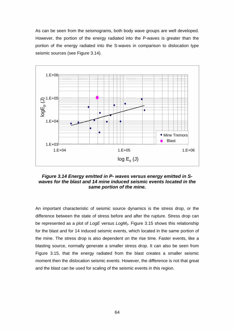
64
As can be seen from the seismograms, both body wave groups are well developed.
However, the portion of the energy radiated into the P-waves is greater than the
portion of the energy radiated into the S-waves in comparison to dislocation type
seismic sources (see Figure 3.14).
1.E+03
1.E+04
1.E+05
1.E+06
1.E+04 1.E+05 1.E+06
log Es (J)
logE
p (J
)
Mine TremorsBlast
Figure 3.14 Energy emitted in P- waves versus energy emitted in S-waves for the blast and 14 mine induced seismic events located in the
same portion of the mine.
An important characteristic of seismic source dynamics is the stress drop, or the
difference between the state of stress before and after the rupture. Stress drop can
be represented as a plot of LogE versus LogM0. Figure 3.15 shows this relationship
for the blast and for 14 induced seismic events, which located in the same portion of
the mine. The stress drop is also dependent on the rise time. Faster events, like a
blasting source, normally generate a smaller stress drop. It can also be seen from
Figure 3.15, that the energy radiated from the blast creates a smaller seismic
moment then the dislocation seismic events. However, the difference is not that great
and the blast can be used for scaling of the seismic events in this region.
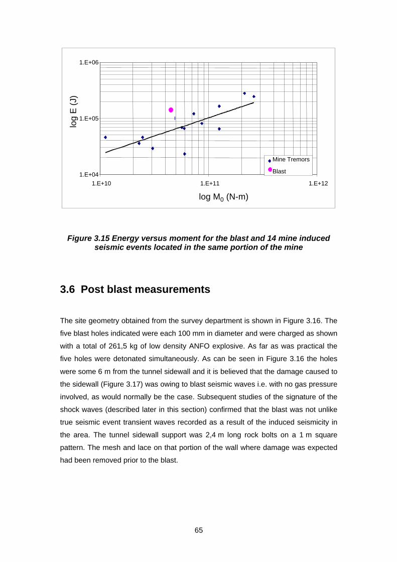
65
1.E+04
1.E+05
1.E+06
1.E+10 1.E+11 1.E+12
log M0 (N-m)
log
E (
J)
Mine Tremors
Blast
Figure 3.15 Energy versus moment for the blast and 14 mine inducedseismic events located in the same portion of the mine
3.6 Post blast measurements
The site geometry obtained from the survey department is shown in Figure 3.16. The
five blast holes indicated were each 100 mm in diameter and were charged as shown
with a total of 261,5 kg of low density ANFO explosive. As far as was practical the
five holes were detonated simultaneously. As can be seen in Figure 3.16 the holes
were some 6 m from the tunnel sidewall and it is believed that the damage caused to
the sidewall (Figure 3.17) was owing to blast seismic waves i.e. with no gas pressure
involved, as would normally be the case. Subsequent studies of the signature of the
shock waves (described later in this section) confirmed that the blast was not unlike
true seismic event transient waves recorded as a result of the induced seismicity in
the area. The tunnel sidewall support was 2,4 m long rock bolts on a 1 m square
pattern. The mesh and lace on that portion of the wall where damage was expected
had been removed prior to the blast.

66
Figure 3.16 Geometry of the controlled seismic source experiment site.
3.6.1 Tunnel wall damage
It was correctly predicted that the general geology in the area and the fracturing in
the vicinity of the excavation would play an important role in governing the nature and
extent of the damage to the tunnel wall. Detailed mapping of the aforementioned was
therefore done (Reddy, 1998).
Mining of the Vaal Reef was in progress at the time of the experiment some 100 m
NNW of the site on the west side of the fault shown in Figure 3.16. This is a normal
fault, dipping east and downthrowing the Vaal Reef 100 m on the eastern side. The
rocks at the site are comprising the hangingwall of the Vaal Reef and are
argillaceous quartzites of the Strathmore Formation known locally as the MB2.
Bedding is visible throughout the area and is generally planar with thicknesses
ranging from 50 to 500 mm. Dips steepen as one gets closer to the fault, most
probably as a result of drag during the faulting process.

67
The argillaceous quartzites are relatively weak. Three tests revealed an average
uniaxial strength of 129 MPa (Drescher, 1998). MINSIM modelling showed a field
stress at the site of 50 MPa, only 19 percentile than the virgin stresses of 42 MPa
(LeBron, 1998). The increase is as a result of the mining mentioned earlier.
“Bow wave” fractures formed during the development of the tunnel. They define
angles of up to 20 degrees to the sidewall. Dips are steep, ranging between 850 and
900. As with the bedding they occur all along the tunnel. Their position with respect to
the tunnel is illustrated in one small zone in Figure 3.16.
The bedding, “bow wave” fractures and rockbolt support all played an important role
in controlling the distribution of damage as a result of the shock waves (Le Bron and
Haile, 1998b). This can be seen in Figure 3.17, which is a collage of photographs of
a portion of the damaged wall. The wall was whitewashed before the blast so the
dark areas on the collage show the areas where rock has been ejected. A rockbolt
can be seen containing some of the whitewashed rock. Many damaged areas have
boundaries defined by the bedding. The “bow wave” fractures often defined other
boundaries and block thicknesses in some cases.
Petroscope studies in holes drilled perpendicular to the tunnel wall revealed that new
tensile fractures had developed within 1m of the tunnel wall. These were clean, wavy,
less than 1 mm wide and aligned parallel to the tunnel wall. In some cases these
planes bounded the ejected blocks.
The dimensions of all ejected blocks with lengths greater than 300 mm were
measured. The volume of each of the blocks was estimated and then accumulated
for every metre along the tunnel wall. The result is shown in Figure 3.18. Relate this
to the reference tape indicated in Figure 3.18 and it can be seen that most of the
damage was sustained directly opposite the charges in the blast holes i.e. between
9 m and 19 m on the tape. The cut off at 9 m was sharp. There was damage beyond
19 m, however, i.e. up to 9 m ahead of the severely damaged area on the tunnel
wall. The solid line in Figure 3.18 is a moving average curve of the damage as
reflected by the volume of ejected blocks.

68
Figure 3.17 Photograph of a portion of the damaged sidewall. A rockboltcan be seen in the top centre.

69
Damage to tunnel w.r.t. position of blast
0
0.02
0.04
0.06
0.08
0.1
0.12
0.14
0.16
0.18
0 1 2 3 4 5 6 7 8 9 10 11 12 13 14 15 16 17 18 19 20 21 22 23 24 25 26 27 28 29 30
Distance along tunnel (m)
Vo
lum
e o
f ro
ck d
isp
lace
d p
er m
eter
(m
*3/m
)
Figure 3.18 Volume of rock ejected along the tunnel wall.
A comparison of ground penetrating radar (GPR) scans taken before and after the
blast showed the development of new fractures in the vicinity and ahead of the blast
holes themselves. The scans also showed the possibility of the development and
opening of fractures close and parallel to the tunnel wall. The latter formed as a result
of the interaction of the seismic waves with the surface of the excavation as would be
the case in a rockburst. Figure 3.19 is an example of an “after blast” scan that probes
9 m into the rock mass i.e. beyond the blast holes. The fracturing described above
can clearly be seen. All the “before blast” scans showed were indistinct indications of
the “bow wave” fractures described earlier. A total of 15 scans were done (Grodner,
1998).
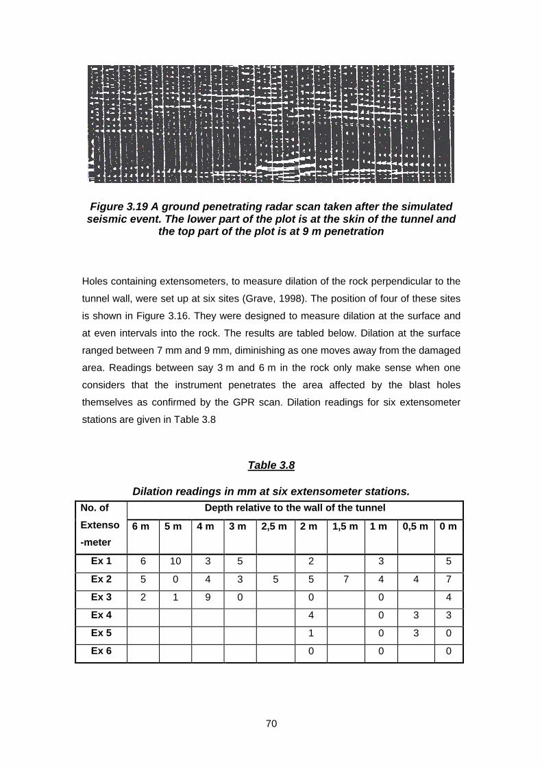
70
Figure 3.19 A ground penetrating radar scan taken after the simulatedseismic event. The lower part of the plot is at the skin of the tunnel and
the top part of the plot is at 9 m penetration
Holes containing extensometers, to measure dilation of the rock perpendicular to the
tunnel wall, were set up at six sites (Grave, 1998). The position of four of these sites
is shown in Figure 3.16. They were designed to measure dilation at the surface and
at even intervals into the rock. The results are tabled below. Dilation at the surface
ranged between 7 mm and 9 mm, diminishing as one moves away from the damaged
area. Readings between say 3 m and 6 m in the rock only make sense when one
considers that the instrument penetrates the area affected by the blast holes
themselves as confirmed by the GPR scan. Dilation readings for six extensometer
stations are given in Table 3.8
Table 3.8
Dilation readings in mm at six extensometer stations.Depth relative to the wall of the tunnelNo. of
Extenso
-meter
6 m 5 m 4 m 3 m 2,5 m 2 m 1,5 m 1 m 0,5 m 0 m
Ex 1 6 10 3 5 2 3 5
Ex 2 5 0 4 3 5 5 7 4 4 7
Ex 3 2 1 9 0 0 0 4
Ex 4 4 0 3 3
Ex 5 1 0 3 0
Ex 6 0 0 0
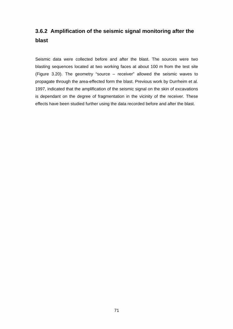
71
3.6.2 Amplification of the seismic signal monitoring after the
blast
Seismic data were collected before and after the blast. The sources were two
blasting sequences located at two working faces at about 100 m from the test site
(Figure 3.20). The geometry “source – receiver” allowed the seismic waves to
propagate through the area-effected form the blast. Previous work by Durrheim et al.
1997, indicated that the amplification of the seismic signal on the skin of excavations
is dependant on the degree of fragmentation in the vicinity of the receiver. These
effects have been studied further using the data recorded before and after the blast.
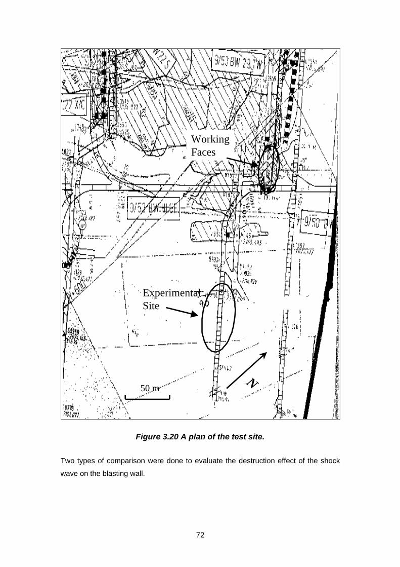
72
N
WorkingFaces
ExperimentalSite
50 m
Figure 3.20 A plan of the test site.
Two types of comparison were done to evaluate the destruction effect of the shock
wave on the blasting wall.

73
A comparison of the maximum velocities in the time domain recorded before and
after the blast (Geophones C1 to C8 from site “C”, Figure 3.1) indicated a five to six
folds amplification of the velocities recorded after the blast. (Compare Figure 3.21 -
before the blast to Figure 3.22 - after the blast). The only exception is the footwall
channel, which was probably less affected by the blast wave or the ground between
the rock and the geophone, acted as a damping filter on the incoming seismic waves.
PPV's measured before the blast
0.01
0.1
1
0 5 10 15 20
Events number
PP
V [m
m/s
]
HW HW HW FW
SW SW SW
Figure 3.21 Peak particle velocities measured on the blasting wall, thehangingwall and the footwall before the main blast.

74
PPV's measured after the blast
0.1
1
10
0 10 20 30 40 50 60 70 80
Events number
PP
V [m
m/s
]
HW HW HW FW
SW SW SW
Figure 3.22 Peak particle velocities measured on the blasting wall, thehangingwall and the footwall after the main blast.
A second comparison was done using the spectral ratio between two geophones
placed normal to the blasting wall at C5 and C8, using method described by
Spottiswoode et al., 1997. The first geophone was closer to the blast and almost at
the end of the area of low intensity damage, while the second geophone was 12 m
from the first one and further away from the blast, in the area where the damage was
not severe.
The maximum velocities recorded before the blast for both the close and the distant
geophones were in the range of 0,1 mm/s to 1,0 mm/s and they did not differ
significantly from each other Figure 3.23. After the blast the values of the maximum
velocities recorded on the closest geophone were 2 to 3 times higher than the
velocities recorded at the distant geophone (Figure 3.24). It can be also seen that the
velocities recorded at the distant geophone remained almost unchanged.

75
Before the Blast
0.0
0.1
0.2
0.3
0.4
0.5
0.6
0.7
0.8
0 5 10 15 20 25 30
Events Number
mm
/s close
far
Figure 3.23 Peak particle velocities measured on the blasting wall beforethe main blast.
After the Blast
0.0
0.5
1.0
1.5
2.0
2.5
3.0
0 20 40 60 80
Events Number
mm
/s close
far
Figure 3.24 Peak particle velocities measured on the blasting wall afterthe main blast.

76
It is also interesting to note how these changes are distributed in the frequency
domain. Figure 3.25 represents a Log10 amplitude spectral ratio for the seismic
events recorded at the closer to the distant geophone, before the blast (It can be
seen that the amplitude spectral ratio between the geophones is approximately 1,0 at
all frequency). Figure 3.26 shows the same spectral ratio but calculated for the
events after the blast. The amplification of the signal for the closer geophone is about
10 times on average over the frequency range of 0 Hz 400 Hz and in the low
frequency domain even greater.
This result is of interest with respect of support design criteria for rockburst
conditions. Frequency less than 100 Hz are expected for larger, potentially damaging
events.
Before the Blast
-0.2
-0.1
0.0
0.1
0.2
0.3
0.4
0.5
0 50 100 150 200 250 300 350 400
Frequency [Hz]
Spe
ctra
l Rat
io L
og(c
lose
/far)
Figure 3.25 A Log10 amplitude spectral ratio, closer to distant geophonefor seismic events recorded at the blasting wall, before the blast.
77
After the Blast
0.00.20.40.60.81.01.21.41.61.82.0
0 100 200 300 400
Frequency [Hz]
Log 1
0 sp
ectr
al r
atio
(cl
ose/
far)
Figure 3.26 A Log10 amplitude spectral ratio for the seismic eventsrecorded at the blasting wall, closer geophone to the distant one, after
the main blast.
The results obtained so far indicate that there is significant amplification of the peak
particle velocities when the seismic wave is propagating through the fractured rock.
This analysis has profound implication and needs further study.
3.7 Conclusions
Some of the important findings are listed below:
• The distance of the blast holes from the tunnel wall ensured that no gas
pressure was directly involved in damaging the wall of the tunnel. The
damage resulted from the interaction of the blast wave with the tunnel, as
would happen in a rockburst. Extensiometer probes and ground penetrating
radar scans confirmed the development of new fractures close to and parallel
to the damaged tunnel wall.

78
• Two areas of damage were identified on the blasting wall:
Ø area with high intensity damage: ground velocity at 3,3 m/s was
recorded by an accelerometer ejected with a block of rock
Ø area with low intensity damage: ground velocity at 1,6 m/s was
recorded by an accelerometer which remained in the tunnel wall
• High speed filming revealed rock fragments being ejected from the wall at
velocities in the range of 0,7 m to 2,5 m per second. The measurements were
taken in the area of low intensity damage.
• The maximum velocity recorded in the solid rock close to the blast was
compared to the velocities recorded on the blasting wall. Ratios were
established of 2,2 times, between the solid rock and the area with high
intensity damage and ratio of 1,3 times between the solid rock and the area
with low intensity damage, after correcting for R-1/2, geometric attenuation in
the near field.
• The attenuation of maximum velocities for the main blast as a function of
distance R was found to follow the law of 1/R1,7.
• The simulated rockburst was recorded by the Vaal River Operations regional
seismic network. The local magnitude was estimated as ML = 1,3. Further use
of the simulated rockburst for scaling of mine tremors located in this region is
recommended.
• Peak particle velocities (PPV’s) were measured on the tunnel wall both before
and after the experimental blast. The PPV’s were as a result of normal mining
operations some 100 m from the site. The PPV’s after the blast were
amplified some five to six times, that recorded before the blast indicating the
effect of damage caused to the rock surrounding the excavation.
• In the frequency domain well defined amplification in excess of ten fold was
obtained in the low frequency band (0 – 100 Hz)
• The new fractures together with both natural bedding planes and “bow wave”
fractures formed during the development of the tunnel determined the shape
of blocks ejected from the wall at the time of the simulated rockburst.
• Tendon support of the tunnel had the effect of reducing the PPV’s and
damage to the wall in their immediate vicinity.
• It was found that the failure of the rock occurred predominantly on prominent
discontinuities such as bedding planes and fractures. Damage to a tunnel is
changed in the presence of discontinuities and this fact should be taken into
account when support is designed.
79
4 Dynamic behaviour of the rock around
underground excavations
4.1.1 Introduction
Measurements of the site response made during the past three years have shown
that the phenomenon of the dynamic site response is real and significant. Many
interesting results have been obtained. For example, it was found that the peak
particle velocity on the skin of the excavation may be amplified four to ten fold
compared to a point in solid rock a similar distance from the focus, and the total
energy flux by even larger amounts. Ground motion at points less than a metre apart
show differences in amplitude and phase which can only be accounted for by large
strain across fractures. A case has been recorded where this behaviour changed
dramatically following a nearby seismic event, suggesting that a significant change in
of stress occurred. The data were initially analysed using classical seismological
approaches such as spectral ratios. Time domain approaches, such as deconvolution
and system identification using data adaptive filters, were also investigated. Latterly,
analysis techniques used by earthquake engineers such as single and multi-mode
harmonic oscillators have been applied.
Much scope exists for the application of concepts from earthquake engineering to the
study of rockburst damage mechanisms and rockburst resistant design. Initially the
project focused only on the motions of the rock. Insights gained from the earthquake
engineering literature suggested that the entire rock support system should be
analysed. This formed an important component of the project.
4.1.2 Site description.
Two sites on Carbon Leader stoping at Western Deep Levels, East Mine – panel
93 E4 were chosen for underground monitored in collaboration with project GAP 330.
Figure 4.1 illustrates the position of the sites and the mining environment.

80
N
50 m
91 E1
93 E4
93 E3
Y -45 6
00X +25 800
Boulder South fault pillar
Mining direction
2D seismic array
3D seismic array
90 Level
94 Level
Figure 4.1 Mining plan and position of the test sites.
The discontinuities include joints, faults, bedding and parting planes together with
mining induced fractures.
Three major joint sets, throwing a north-north-east, a east-west trending and a north-
west were measured. They extend for up to 1 m and are 1 to 3 cm thick. Faults
striking north-east, sub-parallel to the dominant joint set. The faults are all normal
with throws of less than 1 m and dip steeply to the south.
A well-defined argillaceous bed locally defines the base of the Rice Pebble Marker
(found below the Green Bar). The base also occurs as a welded plane with a thin
argillite veneer. This variation may be owing to sedimentological control as well as
selective bedding parallel movement along the plane.

81
Mining-induced fractures have been grouped into extension and shear fractures.
Extension fractures occur as discrete, persistent fractures. Dips are steep (700-850),
but generally less than those of the shear fractures. Orientation is generally face
parallel. Spacing between extension fractures increases near shear fractures and
faults typically 2-10 cm but. Between shear fractures the spacing is 15-25 cm. Shear
fractures occur as zones of intensely fractured rock up to 15 cm wide along which
some displacement has occurred. Spacing of the shear fractures varies between
1,6 m and 2,0 m.
A representative stratigraphic column is presented in Figure 4.2. The footwall
consists of a green-grey, poorly sorted, very coarse grained, immature quartzite.
Glassy, cleaner quartzites occur locally. Persistent, argillaceous parting planes are
up to 20 mm thick and strongly laminated. Impersistent, argillaceous parting planes
are 20-30 cm apart and up to 4 mm thick and also strongly laminated. The thicker
argillaceous parting planes have smooth, shiny bottom contacts indicating movement
along the planes. A 5-10 cm thick medium pebble conglomerate occurs
approximately 50 cm below the Carbon Leader and another similar conglomerate up
to 170 cm below the Carbon Leader.
Carbon Leader
North Leader
Carbon Leader hangingwall
Carbon Leader footwall
Green Bar
Green Bar hangingwall
2 m
0.8-2.0 m
Figure 4.2 Stratigraphic column of the Carbon Leader.
82
The Carbon Leader is a narrow conglomerate up to 12 cm in thickness. It has an
erosive base, often eliminating the argillite parting directly below it.
The Green Bar, an argillaceous unit up to 2,5 m thick, overlies the Rice Pebble
Marker. The Green Bar lies at an average of 2,0 m above the Carbon Leader. Local
tectonic rolls and erosional features may reduce the quartzite parting to 1,2 m. The
base of the Green Bar is characterised by a smooth, polished, tectonised undulating
surface. A well-bedded, often pyritic siltstone occurs at the base, grading into a less
well-bedded chloritoid shale. Fault gouge and vein quartz may occur locally on the
bottom contact.
The Carbon Leader reef is being mined on strike by a conventional 25 m long panel.
Until recently the stope used backfill as permanent support and Camlok props as
temporary face area support. Permanent support has been replaced with elongates
(initially cone props with a later switch to Madodas and then Eben Haeser) and packs
without backfill.
The stope is being mined on strike, and the majority of hangingwall fractures are
oriented between face-parallel and 200 oblique to the stope face, with a moderate to
steep dip.
4.1.3 Method of observation
Following previous results we focussed on the analysing the difference in ground
motion at closely spaced points.
The dynamic response was represented as an amplitude spectral ratio R’(f) and
phase difference δ (f) between two seismic signals measured at different points in the
panel (Spottiswoode et al., 1997).

83
To compare the ground motion at different sites (e.g. A and B), the full waveforms
were Fourier transformed:
)()( ~ ft VV AA⇔ and )()( ~ ft VV BB
⇔ (4.1)
where: )( tV A and )(tV B
are the ground motion time histories and )(~ fV A and
)(~ fV B
are their Fourier transformations.
The ratio of the complex spectrum at each frequency was expressed as amplitude
ratio A(f) and phase difference δ(f):
))(i 2exp()()(/)( ~~ ffAff VV ABδπ= (4.2)
where: A(f) is an amplitude ratio and δ(f) is the phase difference:
Spectral values may vary widely and give a noisy appearance. Spectral ratios, such
as A(f) in Equation (4.2), are more prone to noise. To obtain stable values, spectra
for many events were obtained and the median used, R′(f) and δ′(f), of all spectral
components for A(f) and δ(f) at each frequency. After replacing amplitude ratio’s and
the phase differences with their median values, averaged for number of events, the
Equation (4.2) can be written as:
))('i 2exp()(')(/)( ~~ ffRff VV ABδπ= (4.3)
The phase difference, δ’(f), was interpreted in terms of the propagation velocity of
seismic energy. This provides some insights into the “softening” effect of the fracture
zone around the stope. These analyses have suggested that the effective velocities
of propagation are much less than the S-wave velocity.
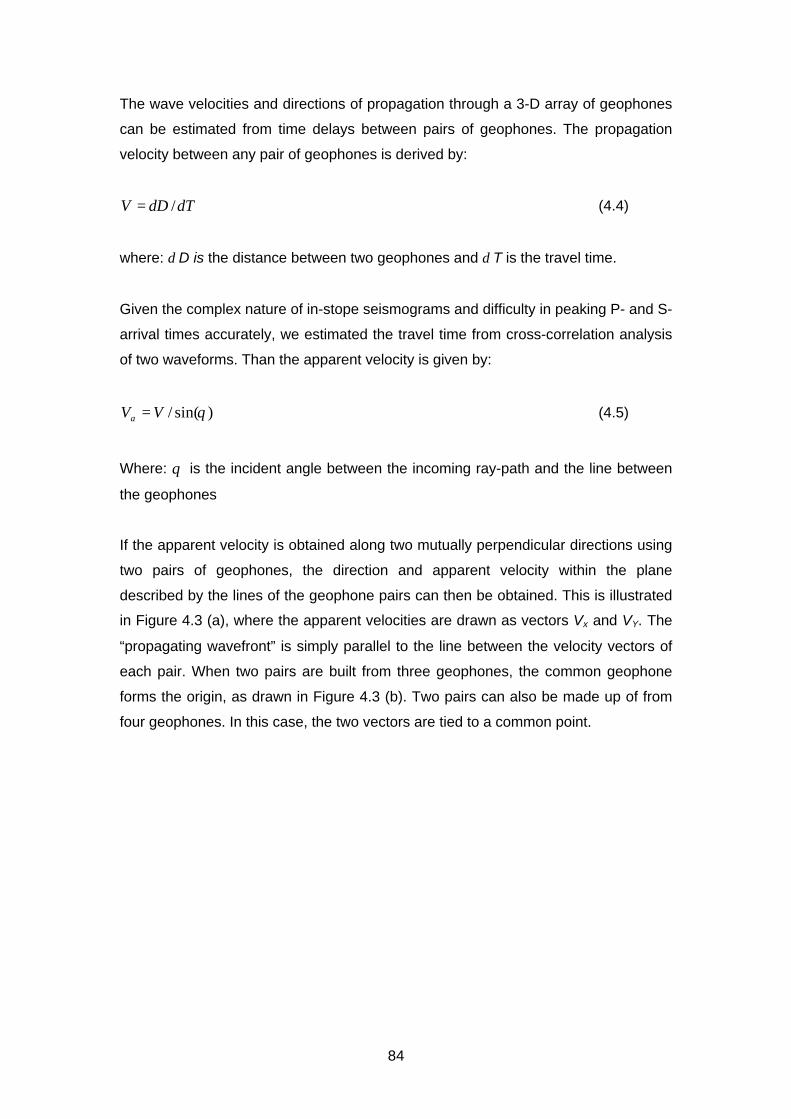
84
The wave velocities and directions of propagation through a 3-D array of geophones
can be estimated from time delays between pairs of geophones. The propagation
velocity between any pair of geophones is derived by:
TDV δδ /= (4.4)
where: δ D is the distance between two geophones and δ T is the travel time.
Given the complex nature of in-stope seismograms and difficulty in peaking P- and S-
arrival times accurately, we estimated the travel time from cross-correlation analysis
of two waveforms. Than the apparent velocity is given by:
)sin(/ θVVa = (4.5)
Where: θ is the incident angle between the incoming ray-path and the line between
the geophones
If the apparent velocity is obtained along two mutually perpendicular directions using
two pairs of geophones, the direction and apparent velocity within the plane
described by the lines of the geophone pairs can then be obtained. This is illustrated
in Figure 4.3 (a), where the apparent velocities are drawn as vectors Vx and VY. The
“propagating wavefront” is simply parallel to the line between the velocity vectors of
each pair. When two pairs are built from three geophones, the common geophone
forms the origin, as drawn in Figure 4.3 (b). Two pairs can also be made up of from
four geophones. In this case, the two vectors are tied to a common point.
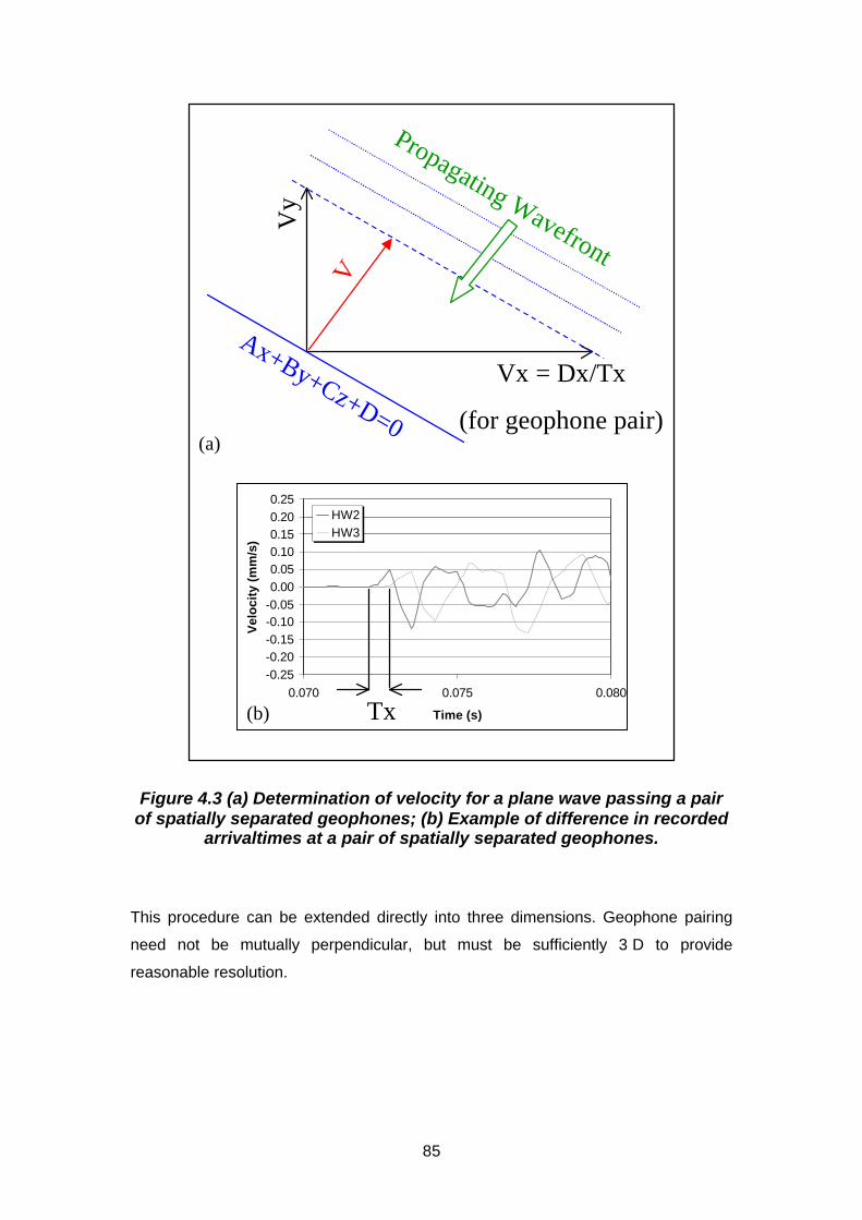
85
Vy
VAx+By+Cz+D=0
Propagating Wavefront
Vx = Dx/Tx
(for geophone pair)(a)
-0.25-0.20-0.15-0.10-0.050.000.050.100.150.200.25
0.070 0.075 0.080
Time (s)
Vel
oci
ty (
mm
/s)
HW2HW3
Tx(b)
Figure 4.3 (a) Determination of velocity for a plane wave passing a pairof spatially separated geophones; (b) Example of difference in recorded
arrivaltimes at a pair of spatially separated geophones.
This procedure can be extended directly into three dimensions. Geophone pairing
need not be mutually perpendicular, but must be sufficiently 3 D to provide
reasonable resolution.

86
4.1.4 Analysis of peak particle velocities
4.1.4.1 Up-hole micro seismic array (3 D observations)
A linear array of triaxial geophones connected to a Portable Seismic System (PSS)
was installed into a 10 m long hole drilled vertically into the hangingwall. Each of the
five triaxial sites was separated from its nearest neighbour by 2 m, with the lowest
geophone being positioned into the hangingwall. In addition, a surface array of
uniaxial geophones connected to a ground motion monitor (GMM) was installed on
the skin of the hangingwall in the immediate vicinity of the hole. The PSS and GMM
shared a common channel, to confirm consistency of system calibration and facilitate
to combination of the data sets from these two systems (Figure 4.4).
The lowest triaxial geophone was installed just below the bottom the Green Bar
interface, while the next geophone was installed above the Green Bar interface. The
other three triaxial geophones and the surface vertical geophones are all located in
quartzite hangingwall strata above the Green Bar.
A preliminary estimate of wave velocities in the vicinity of up-hole array (Figure 4.4),
is presented in GAP 330 report. The velocity values in the range of 500 m/s to
700 m/s were obtained. These were confirmed by direct measurements from a
hammer blow source where the numbers are quite variable from event to event and
are also so much lower than the P- and S- velocities for solid rock taken as 5800 m/s
for P- and 3700 m/s for S- wave. As values much less than those for solid rock have
profound implication for our understanding of the rock mass dynamic behaviour.
These results were further re-evaluated for a paper in preparation (Milev et al., 1998).

87
SECTION VIEW
PSS0
A
B
C
D
GULLY“THE OCTOBOX”PSS DAU
PLAN VIEW(configuration I)
HOLE HW2
HW4
HW3
HW5
HW6FW7 FW8LG
HOLEHW2
HW4HW3
HW5
HW6
FW7
FW8LG
PLAN VIEW(configuration II)
Figure 4.4 Plan and sectional view of 3 D micro seismic networkinstalled at WDL, East Mine, 93E4 panel: configuration I, operated from
January ’98 to May ’98; configuration II has operated since May ’98.
Some 521 common events were identified as having been recorded by both the PSS
and the GMM, and the data files were combined for joint assessment. All detailed
analysis was conducted using the combined data.
Some repeatable characteristics which had been observed in the PSS waveforms –
notably, the apparent azimuth angles between source and receiver derived from the
known polarisation characteristics of the P-wave first arrivals – were used to group
the data into various clusters. The mine’s data were then used to associate the
clusters with specific source regions (e.g. the 93 Level stope faces to the north east
of the recording site, which were steadily advancing away from the site during the
period of recording).
It was found that data recorded from seismic events on 90 Level (to the west of the
site) tended to have dominant P-wave amplitude on the east-west horizontal
component. Travel times for these seismic waves tended to be shorter than expected
from the assumed rock mass velocities. The waves recorded on the geophones

88
closer to the hangingwall surface arrived with a noticeable delay compared with
those further into the hangingwall.
Data recorded from seismic events on 93 Level (to the north east of the site –
associated with stope faces closest to the site) tended to have similar P-wave
amplitudes on both the north-south and east-west horizontal components. Travel
times tended to be more or less consistent with the expectations. There was
generally negligible delay in arrival of the waves at the geophones at various depths
into the hangingwall.
Data recorded from seismic events on 94 Level (to the east of the site, at similar
distances as those for the 90 Level events) tended to have a dominant P-wave
amplitude on the north-south horizontal component. Travel times for these waves
tended to be noticeably longer than expected. There was typically no measurable
delay in arrival of the waves at the geophones at various depths into the hangingwall.
A visual of the waveforms shows changes in the appearance of the waveforms from
top to bottom through the borehole array.
An increased degree of complication of the signals from top to bottom was
accompanied by an increase in the amplitude and duration of the coda waves (most
probably Rayleigh waves). These effects are indicative of energy trapping within the
fracture zone close to the excavation.
The maximum velocities for the entire data set recorded by the borehole array are
shown in Figure 4.5. Their values ranged from 0,6 mm/s to 5 mm/s. Similar behaviour
with small dispersion was obtained.

89
0.01
0.1
1
10
0.01 0.1 1 10
Site A [mm/s]
A, B
, C &
D [m
m/s
]
A
B
C
D
Family of up-holetrendlines
Figure 4.5 Maximum velocities recorded at site WDL, East mine, 93E4panel, geophones A, B, C and D are installed in the borehole from top to
bottom.
The maximum velocities recorded from the skin of the hangingwall are shown in
Figure 4.6. The variations in velocity from individual events on the skin of the
hangingwall were larger than the variations of velocity within the borehole. Their
values (ranging from 0,2 mm/s to 7 mm/s) are larger than the maximum velocities
recorded in the borehole array.
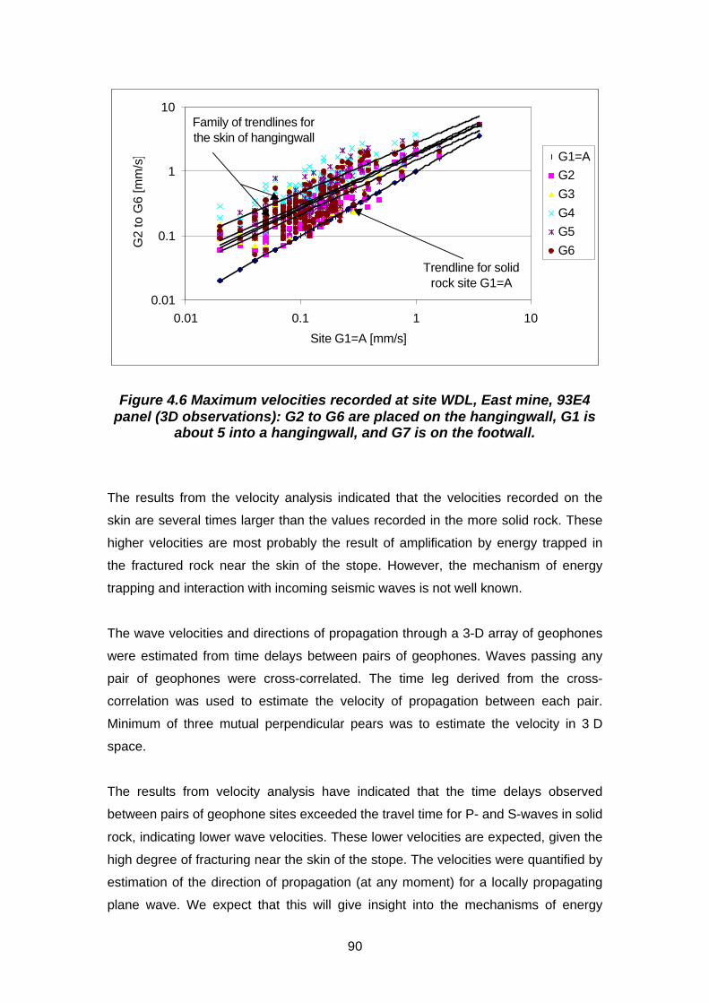
90
0.01
0.1
1
10
0.01 0.1 1 10
Site G1=A [mm/s]
G2
to G
6 [m
m/s
] G1=A
G2
G3
G4
G5
G6
Family of trendlines forthe skin of hangingwall
Trendline for solid rock site G1=A
Figure 4.6 Maximum velocities recorded at site WDL, East mine, 93E4panel (3D observations): G2 to G6 are placed on the hangingwall, G1 is
about 5 into a hangingwall, and G7 is on the footwall.
The results from the velocity analysis indicated that the velocities recorded on the
skin are several times larger than the values recorded in the more solid rock. These
higher velocities are most probably the result of amplification by energy trapped in
the fractured rock near the skin of the stope. However, the mechanism of energy
trapping and interaction with incoming seismic waves is not well known.
The wave velocities and directions of propagation through a 3-D array of geophones
were estimated from time delays between pairs of geophones. Waves passing any
pair of geophones were cross-correlated. The time leg derived from the cross-
correlation was used to estimate the velocity of propagation between each pair.
Minimum of three mutual perpendicular pears was to estimate the velocity in 3 D
space.
The results from velocity analysis have indicated that the time delays observed
between pairs of geophone sites exceeded the travel time for P- and S-waves in solid
rock, indicating lower wave velocities. These lower velocities are expected, given the
high degree of fracturing near the skin of the stope. The velocities were quantified by
estimation of the direction of propagation (at any moment) for a locally propagating
plane wave. We expect that this will give insight into the mechanisms of energy

91
trapping that result in the pronounced coda waves. It will also assist in estimating the
effective stiffness of the fractured rock and, thereby, it’s dynamic response.
4.1.4.2 In-stope measurements of the peak particle velocities (2 D seismic
array)
Two additional Ground Motion Monitors with a common trigger and 15 geophones
were installed as part of the in-stope monitoring program described above. The site
location is shown in Figure 4.1. The recording configuration is represented in
Figure 4.7. Most of the geophones were placed on the hangingwall except B5, B6
and B7, which were deployed on the footwall.
Quasi-static instrumentation consisting of a closure ride station, extensometer,
tiltmeter crack gauge and doorstopper was installed in the area covered by the
ground motion monitors. We had hoped to use these data to divide the time plot into
stages, for example, high and low stress, or different deformation rates. Unfortunately
no clear pattern showing different stages were available from the quasi-static
instrumentation. Details on the quasi-static measurements can be find in GAP 330.

92
FACE
B8LG
GULLYTWO BOXES WITH COMMON TRIGGER
ACQUISITION UNIT
AB3
A8LGA2
B4
B2B1B5FW
B6FW B7FW
QUASISTATIC
BA
TRIGGER
FA
ULT
A5A4
A7
A6
A1
SECTION
PLAN
800
N
Figure 4.7 Configuration of micro seismic array consisting of twoground motion monitors (A & B) with a common trigger and 15
geophones. All geophones are on the hangingwall except B5, B6 and B7which are located on the footwall.
The maximum velocities recorded at site A are shown in Figure 4.8. An interesting
feature for this site was the northeasterly trending fault that cut through the mini
network. The geophones A1, A4, A6 and A7 were on the North side of the fault while
the geophones A2, A5, A3 and A8 were on the South side of the fault. Geophones
A8 and B8 were reserved for strong seismic events and set on low gain only.
Geophone A7 had poor signal characteristics. Geophones A7 and A8 have been
excluded from the analysis.
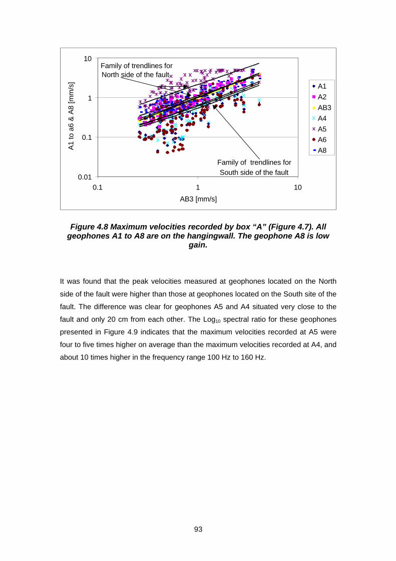
93
0.01
0.1
1
10
0.1 1 10
AB3 [mm/s]
A1
to a
6 &
A8
[mm
/s]
A1
A2
AB3
A4
A5
A6
A8
Family of trendlines for South side of the fault
Family of trendlines forNorth side of the fault
Figure 4.8 Maximum velocities recorded by box “A” (Figure 4.7). Allgeophones A1 to A8 are on the hangingwall. The geophone A8 is low
gain.
It was found that the peak velocities measured at geophones located on the North
side of the fault were higher than those at geophones located on the South site of the
fault. The difference was clear for geophones A5 and A4 situated very close to the
fault and only 20 cm from each other. The Log10 spectral ratio for these geophones
presented in Figure 4.9 indicates that the maximum velocities recorded at A5 were
four to five times higher on average than the maximum velocities recorded at A4, and
about 10 times higher in the frequency range 100 Hz to 160 Hz.
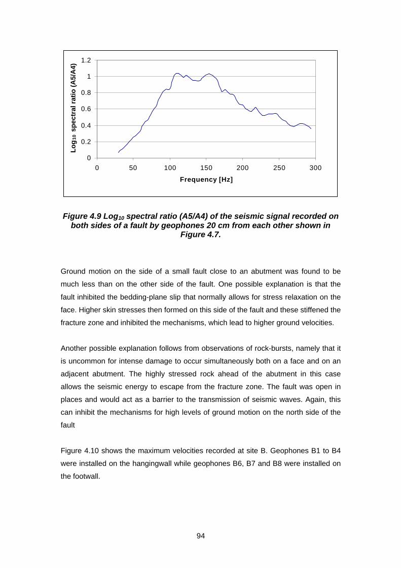
94
0
0.2
0.4
0.6
0.8
1
1.2
0 50 100 150 200 250 300
Frequency [Hz]
Lo
g10 s
pec
tral
rat
io (
A5/
A4)
Figure 4.9 Log10 spectral ratio (A5/A4) of the seismic signal recorded onboth sides of a fault by geophones 20 cm from each other shown in
Figure 4.7.
Ground motion on the side of a small fault close to an abutment was found to be
much less than on the other side of the fault. One possible explanation is that the
fault inhibited the bedding-plane slip that normally allows for stress relaxation on the
face. Higher skin stresses then formed on this side of the fault and these stiffened the
fracture zone and inhibited the mechanisms, which lead to higher ground velocities.
Another possible explanation follows from observations of rock-bursts, namely that it
is uncommon for intense damage to occur simultaneously both on a face and on an
adjacent abutment. The highly stressed rock ahead of the abutment in this case
allows the seismic energy to escape from the fracture zone. The fault was open in
places and would act as a barrier to the transmission of seismic waves. Again, this
can inhibit the mechanisms for high levels of ground motion on the north side of the
fault
Figure 4.10 shows the maximum velocities recorded at site B. Geophones B1 to B4
were installed on the hangingwall while geophones B6, B7 and B8 were installed on
the footwall.

95
0.01
0.1
1
10
0.1 1 10
AB3 [mm/s]
B1
to B
7 [m
m/s
]B1:HW
B2:HW
AB3:HW
B4:HW
B5:FW
B6:FW
B7:FWFamily of footwall
trendlines
Family of hangingwalltrendlines
Figure 4.10 Maximum velocities recorded by box “B” (Figure 4.7).Geophones B1 to B4 and B8 are placed on the hangingwall. Geophones
B5 to B7 are on the footwall. Geophone B8 is low gain
Peak velocities were used to look at the relative motion between hangingwall and
footwall. This shows independent behaviour between the two, as has been observed
before.
4.1.5 Dynamic response of the hangingwall observed
by 3 D micro seismic array.
The dynamic behaviour of the rock mass surrounding the Up-hole site has been
analysed in terms of spectral ratio. The three-dimensional seismic network installed
there provides an excellent opportunity to examine the change in the seismic wave
close to an underground opening.
Figure 4.11 shows the Log10 amplitude spectral ratio of the seismic signal recorded at
6,5 m into solid rock (G1) and a number of seismic signals recorded at the skin of the
excavation (G2, G3, G4, G5 and G6) for Configuration I from Figure 4.4. We suggest
that G1 (6,5 m into the borehole) closely represent the solid rock.

96
WDL East, panel 93 E4 (configuration I)
-0.2
0
0.2
0.4
0.6
0.8
1
1.2
0 20 40 60 80 100 120 140 160 180 200 220 240 260 280 300Frequency (Hz)
Lo
g10
sp
ectr
al r
atio
s
G2/G1 G3/G1 G4/G1 G5/G1 G6/G1
40 Hz peakstructural response
75 Hz peakstructural response
185 Hz peaklocal effect
Freq. >140 Hz local effect
Figure 4.11 Log10(spectral ratio) of the seismic signal recorded at 6,5 minto the hangingwall (G1) and a number of seismic signals recorded atthe skin of the excavation (G2, G3, G4, G5 and G6) for configuration I
from Figure 4.4.
Two mechanisms of dynamic response have been defined here: structural response,
defined as a common spectral behaviour at all surface seismograms; and local site
effect, defined by spectral peaks at one or two surface seismograms.
Strong structural response was observed in the low frequency range at 40 Hz and
70 Hz for all surface sites (G2 to G6). Local site effects were observed at two surface
sites for frequencies above 140 Hz (G4 and G5), with a clear peak at 185 Hz for G5.
The spectral peaks interpreted as the structural response (40 Hz and 70 Hz for all
surface sites) could be associated with widespread effects, such as the Green Bar
layer, while the site effects observed at G4 and G5 reflect the difference in the
intensity of the local fractures in the vicinity of the geophones.

97
A few months later the geophones G5 and G6 were moved dipper 1 m beyond the
geophone G5. The idea was to trace the size of an anomaly located around G5
(Figure 4.4).
Figure 4.12 shows the spectral ratios between the seismic signals recorded in the
solid rock and seismic signals recorded on the skin of the excavation for this new
configuration (Figure 4.4 - Configuration II).
WDL East, panel 93 E4 (configuration II)
-0.4
-0.2
0
0.2
0.4
0.6
0.8
1
1.2
0 20 40 60 80 100 120 140 160 180 200 220 240 260 280 300
Frequency (Hz)
Lo
g10
sp
ectr
al r
atio
s
G2/G1 G3/G1 G4/G1 G5/G1 G6/G1
45 Hz peakstructural effect
70 Hz peakstructural effect
Frq >200 Hz local effect
180 Hz peakcnversion from local to structural effect
Figure 4.12 Log10(spectral ratio) of the seismic signal recorded in solidrock (G1) and a number of seismic signals recorded at the skin of the
excavation (G2, G3, G4, G5 and G6) for configuration II from Figure 4.4.
It can be seen from Figure 4.12 that the spectral peaks at 40 Hz and 70 Hz for all
surface geophones remained the same as they were before. This indicates that the
expected deterioration in the hangingwall and the support in time, does not effect the
low frequencies.
Significant change is obtained for geophones G2 and G3, which have developed a
spectral peak at 185 Hz. The spectral behaviour for G5 at its’ new position is similar
to G3, G3 and G4 in range of 185 Hz, while the spectral behaviour for G6 is similar to
those of G4 for frequencies higher than 200 Hz. These changes are interpreted as
98
local effect. However, the size of the affected area is apparently larger than the span
of the surface network and cannot be accurately mapped.
The results obtained for the dynamic response of the site, including both the
structural response and the local site effect, can be related to the existing support
methodology. The normalised load-deformation curve, presently used as a support
design criterion, could be modified by the dynamic response spectrum in order to
provide additional design information.
4.1.6 Conclusions
The ground motion at points on the skin of a stope hangingwall was found to be
some four to ten times larger than at a point 6,5 m into the hanging wall. Coda waves
were also more developed on the skin. Measurements at 0,5 m, 2,5 m and 4,5 m
showed intermediate behavior. It was suggested that the fracture zone acting as a
wave-guide causes the enhanced levels of ground motion and that multiple scattering
causes the prolonged duration of motion.
Ground motion on the abutment side of a fault in the hangingwall was much lower
than the ground motion on the other side.
The results from velocity analysis have indicated that the time delays observed
between pairs of geophone sites exceeded the travel time for P- and S-waves, in
solid rock indicating lower wave velocities. These lower velocities are expected,
given the high degree of fracturing near the skin of the stope. It is expected that this
will give insight into the mechanisms of energy trapping. It will also assist in
estimating the effective stiffness of the fractured rock and, thereby, it’s dynamic
response.
Two mechanisms of dynamic response have been defined: structural response,
defined as a common spectral behaviour at all surface seismograms; and local site
effect, defined by spectral peaks at one or two surface seismograms. The spectral
peaks interpreted as the structural response (40 Hz and 70 Hz for all surface sites)
could be associated with the presence of the Green Bar layer in the quartzite, while
the site effects observed at G4 and G5 would be more dependent on the difference in

99
the intensity of the local fractures in the vicinity of the geophones. However, this
interpretation is too broad and numerical modelling is required to provides insights
into the actual mechanism of dynamic behaviour of the hangingwall.
The results obtained for the dynamic response of the site, including both the
structural response and the local site effect, can be related to the existing support
methodology. The normalised load-deformation curve, presently used as a support
design criterion, could be modified by the dynamic response spectrum in order to
provide additional design information.
4.2 Dynamic behaviour of pre-stressed elongates:
underground measurements at Western Deep Levels,
East Mine site
4.2.1 Introduction
One of the objectives of the site response project was to determine the performance
of stope support under dynamic conditions. This kind of study is not a direct
evaluation of the site response, but that of the response of support units under
different conditions. The interaction of the support unit with the hangingwall and the
footwall during the seismic event is still not well understood. Some of the support
units used to support the stope during mining are elongate props. By recording the
motion taking place in the hangingwall, the prop, and the footwall simultaneously, it is
possible to gain better understanding of the interaction between these sites. Because
differences between these sites may be frequency dependent, data analysis was
done in the frequency domain.
4.2.2 Data
An experiment was conducted at Western Deep levels East Mine (93 level E4) to
assess the behaviour of the Eben Haeser prop and the “pencil stick” prop during a

100
seismic event. Figure 4.13 shows a schematic diagram of the experimental set-up.
The diagram shows vertical geophones attached to the hangingwall, the props and
the footwall. The props were separated by about 1,6 m. Thus for seismic
wavelengths of interest the footwall and hangingwall motions should be similar for
both sites. The site was instrumented two weeks after the props were installed.
Therefore, a considerable amount of yielding had taken place and the props were
expected to be supporting close to their maximum load carrying capabilities.
Channels to which the geophones record motion were numbered consecutively from
G1 to G8. A total of 542 events were recorded and analysed. Channel 5, recording
the footwall close to the pencil prop did not perform consistently. This meant that
there was a reduction in the number of events when this channel was included in the
analysis. However there was still enough data to provide a realistic analysis.
Amplitude spectra, spectral ratios between channels, and phase differences were
used as analysis tools.
BB
JB
H/W
F/W
G1
G2
G3
G4
G5
G6
G7
G8
Ebe
n H
aese
rPr
op Penc
il Pr
op
Figure 4.13 A schematic diagram shows the instrumentation of theprops, the footwall and the hangingwall. An 8 channel Ground Motion
Monitor connected to 8 uniaxial vertical geophones was used. Thegeophones were connected to the box via a junction box (JB).
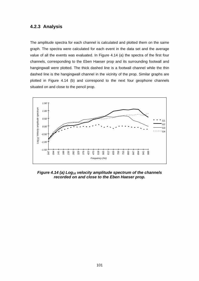
101
4.2.3 Analysis
The amplitude spectra for each channel is calculated and plotted them on the same
graph. The spectra were calculated for each event in the data set and the average
value of all the events was evaluated. In Figure 4.14 (a) the spectra of the first four
channels, corresponding to the Eben Haeser prop and its surrounding footwall and
hangingwall were plotted. The thick dashed line is a footwall channel while the thin
dashed line is the hangingwall channel in the vicinity of the prop. Similar graphs are
plotted in Figure 4.14 (b) and correspond to the next four geophone channels
situated on and close to the pencil prop.
-1.50
-1.00
-0.50
0.00
0.50
1.00
1.50
047
094
141
188
235
282
329
376
423
470
518
565
612
659
706
753
800
847
894
941
988
Frequency (Hz)
Log
10 V
eloc
ity a
mpl
itude
spe
ctru
m
G1
G2
G3
G4
Figure 4.14 (a) Log10 velocity amplitude spectrum of the channelsrecorded on and close to the Eben Haeser prop.

102
-1.50
-1.00
-0.50
0.00
0.50
1.00
1.50
047
094
141
188
235
282
329
376
423
470
518
565
612
659
706
753
800
847
894
941
988
Frequency (Hz)
Log 1
0 V
eloc
ity a
mpl
itude
spe
ctru
m
G5
G6
G7
G8
Figure 4.14 (b) Log10 velocity amplitude spectrum of the channelsrecorded on and close to the pencil prop.
For the Eben Haeser prop the spectra for the hangingwall and the two prop
geophones are similar for frequencies below 560 Hz. The energy increases steadily
with frequency for all of the three channels. This is perhaps representative of the
energy distribution in the input signal. As far as the prop is concerned, the input
signal comes from the combined hangingwall and footwall contributions. It can be
seen that the footwall channel is generally flat from 181 Hz onwards and is of lower
amplitude compared to the other three channels. Above 560 Hz, the prop channel
close to the footwall “seems” to have higher energy than all the channels. This is only
possible when there is constructive interference of the footwall and hangingwall
signals at these frequencies.
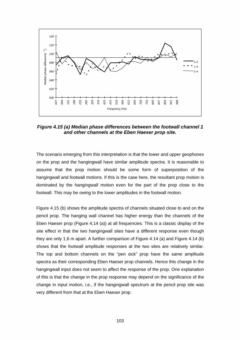
103
000
020
040
060
080
100
120
140
047
094
141
188
235
282
329
376
423
470
518
565
612
659
706
753
800
847
894
941
988
Frequency (Hz)
Med
ian
phas
e di
ffere
nce(
0)
1-2
1-3
1-4
Figure 4.15 (a) Median phase differences between the footwall channel 1and other channels at the Eben Haeser prop site.
The scenario emerging from this interpretation is that the lower and upper geophones
on the prop and the hangingwall have similar amplitude spectra. It is reasonable to
assume that the prop motion should be some form of superposition of the
hangingwall and footwall motions. If this is the case here, the resultant prop motion is
dominated by the hangingwall motion even for the part of the prop close to the
footwall. This may be owing to the lower amplitudes in the footwall motion.
Figure 4.15 (b) shows the amplitude spectra of channels situated close to and on the
pencil prop. The hanging wall channel has higher energy than the channels of the
Eben Haeser prop (Figure 4.14 (a)) at all frequencies. This is a classic display of the
site effect in that the two hangingwall sites have a different response even though
they are only 1,6 m apart. A further comparison of Figure 4.14 (a) and Figure 4.14 (b)
shows that the footwall amplitude responses at the two sites are relatively similar.
The top and bottom channels on the “pen sick” prop have the same amplitude
spectra as their corresponding Eben Haeser prop channels. Hence this change in the
hangingwall input does not seem to affect the response of the prop. One explanation
of this is that the change in the prop response may depend on the significance of the
change in input motion, i.e., if the hangingwall spectrum at the pencil prop site was
very different from that at the Eben Haeser prop.
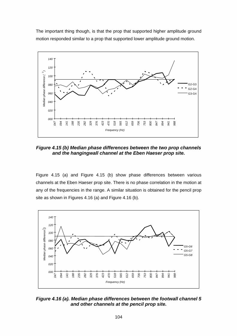
104
The important thing though, is that the prop that supported higher amplitude ground
motion responded similar to a prop that supported lower amplitude ground motion.
000
020
040
060
080
100
120
140
047
094
141
188
235
282
329
376
423
470
518
565
612
659
706
753
800
847
894
941
988
Frequency (Hz)
Med
ian
phas
e di
ffere
nce
(0)
G2-G3
G2-G4
G3-G4
Figure 4.15 (b) Median phase differences between the two prop channelsand the hangingwall channel at the Eben Haeser prop site.
Figure 4.15 (a) and Figure 4.15 (b) show phase differences between various
channels at the Eben Haeser prop site. There is no phase correlation in the motion at
any of the frequencies in the range. A similar situation is obtained for the pencil prop
site as shown in Figures 4.16 (a) and Figure 4.16 (b).
000
020
040
060
080
100
120
140
047
094
141
188
235
282
329
376
423
470
518
565
612
659
706
753
800
847
894
941
988
Frequency (Hz)
Med
ian
phas
e di
ffere
nce
(0)
G5-G6
G5-G7
G5-G8
Figure 4.16 (a). Median phase differences between the footwall channel 5and other channels at the pencil prop site.
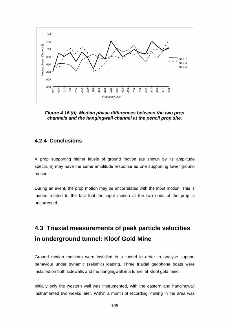
105
000
020
040
060
080
100
120
140
047
094
141
188
235
282
329
376
423
470
518
565
612
659
706
753
800
847
894
941
988
Frequency (Hz)
Med
ian
phas
e di
ffere
nce
(0)
G6-G7
G6-G8
G7-G8
Figure 4.16 (b). Median phase differences between the two propchannels and the hangingwall channel at the pencil prop site.
4.2.4 Conclusions
A prop supporting higher levels of ground motion (as shown by its amplitude
spectrum) may have the same amplitude response as one supporting lower ground
motion.
During an event, the prop motion may be uncorrelated with the input motion. This is
indeed related to the fact that the input motion at the two ends of the prop is
uncorrected.
4.3 Triaxial measurements of peak particle velocities
in underground tunnel: Kloof Gold Mine
Ground motion monitors were installed in a tunnel in order to analyse support
behaviour under dynamic (seismic) loading. Three triaxial geophone boats were
installed on both sidewalls and the hangingwall in a tunnel at Kloof gold mine.
Initially only the western wall was instrumented, with the eastern and hangingwall
instrumented two weeks later. Within a month of recording, mining in the area was

106
stopped. This led to a decrease in the number of seismic events. In three months, 92,
58 and 45 acceptable events were recorded on the eastern western and hangingwall
respectively.
On the hangingwall the two horizontal directions have the same peak velocities.
Unfortunately the vertical component, perpendicular to the hangingwall had
resonance due to poor installation of the geophone.
The eastern and western walls show a very slight difference between the two
tangential components. The component parallel to the length of the tunnel shows
higher peak velocities than the one perpendicular to that direction. Interestingly,
perpendicular components do not show high peak values associated with the free
surface.
4.3.1 Introduction.
A seismic wave may cause damage to all kinds of underground excavations,
including service tunnels. Understanding how the tunnel behaves during a seismic
event may shed light on how best to support the tunnel to sustain dynamic loading.
Since the rock surrounding the excavation is not homogeneous, the seismic
response of the tunnel is expected to vary with position. It is therefore important to
understand these variations in order to understand damage owing to a seismic wave.
To achieve this, factors such as the position of the tunnel with respect to the seismic
event, differences in interaction of waves with different walls of the tunnel, the
frequency content of seismic waves, etc., must be investigated.
A complete description of motion at any point (small volume) in solid ground is
achieved by recording three components of the motion at that point. On the surface
of an excavation, recording motion perpendicular to the ground, and tangential
motion in two mutually orthogonal directions usually achieves this. In this way a
comparison of motion between the three directions at the same site can be made in
order to determine the component that is more diagnostic of seismic damage. This
study attempts to address that aspect of site response. The main parameter used in
this investigation is the peak velocity. For purposes of this study, the peak velocity is
defined as the absolute value of the largest excursion along the seismogram. This

107
means that when two seismograms are compared with each other, the position and
the sign of the peak value are not necessarily the same for both events. This further
assumes that the input signal at a site is the same for all components and that the
differences between the seismograms emanate from the site. However, with surface
recorded Ground Motion Monitor seismograms, it is difficult to separate the P- and S-
waves because most of the triggered events are short distance events which reach
the recording sites before enough P/S separation has taken place. Added to this is
non-linear distortion caused by the fractured zone. It is however thought that the site
effects (despite the presence of source effects and inaccurate peak velocity
estimates) still contribute a great deal to observed differences.
4.3.2 Site description.
A cartoon showing how the experiment was set up is shown in Figure 4.17 (a)
depicting how triaxial geophones were laid out on the surface of the tunnel. Three
triaxial sets were attached to the eastern, western and hanging walls. Each triaxial
geophone set is connected to a separate Ground Motion Monitor. Figure 4.17 (b) is a
plan view of the experimental site, shown as a dashed rectangle, together with its
immediate surroundings. The faces being advancing semi-parallel to the footwall
tunnel being monitored with all mining activity taking place to the East Side of the
tunnel. This led to the assumption that most of the seismic events recorded in
Ground Motion Monitors placed at the experimental site emanate from the eastern
side of the tunnel.

108
Sensor positions inthe tunnel
x
y
z
y
x
z
y
x
z
Mined out
experimental site
Foo
twal
l tun
nel
Soli
d gr
ound
(a) (b)
N
Figure 4.17 Experimental setup (a) showing the cross-section of atunnel with triaxial sensor positions; (b) plan view of the experimentalsite and its surrounding areas. The diagrams are not drawn to scale.
4.3.3 Data
The site had been chosen to assess changes in the response of the tunnel skin to
seismic waves as the tunnel deformed owing to changing stress conditions imposed
by mining of the stope 40 m to the east of the tunnel. Mining advances due south.
Ground motion monitors were placed about 25 m ahead of the approaching mining
face. At first only the western wall of the tunnel was instrumented with the hanging
wall and the eastern wall following two weeks later. Within a few weeks of recording,
the mining stopped in this area. This reduced seismicity. In three months the Ground
Motion Monitor on the eastern wall recorded 92 “good“ events. The western wall and
the hanging wall boxes recorded 58 and 45 “good” events respectively. The lower
number of events being owing to the fact that the latter two boxes were only installed
two weeks after the eastern wall box had been installed. There was no correlation
between events recorded by the seismic network and Ground Motion Monitor events.
Thus location of the Ground Motion Monitor events was not possible.

109
4.3.4 Results
Results from the two sidewalls will be discussed first. Peak velocities of the 3
components of ground motion were plotted on the same graph. The x component,
which is ground motion perpendicular to the sidewall, was used as a reference
component against which the other components were plotted. Figure 4.18 (a) and
Figure 4.18 (b) correspond to eastern and western walls respectively.
Eastern wall
1.00
10.00
100.00
1 10 100
Peak vel., x comp (mm/s)
Pea
k ve
l., x
,y,z
com
p. (
mm
/s)
X
Y
Z
Figure 4.18 (a) Peak velocities of three mutually orthogonal componentsof the eastern sidewall site plotted on the same graph.
Western wall
1.00
10.00
100.00
1.00 10.00 100.00
Peak vel., x comp (mm/s)
Pea
k ve
l., x
,y,z
com
p (m
m/s
)
X
Y
Z
Figure 4.18 (b) Peak velocities of three mutually orthogonal componentsof the western sidewall site plotted on the same graph.
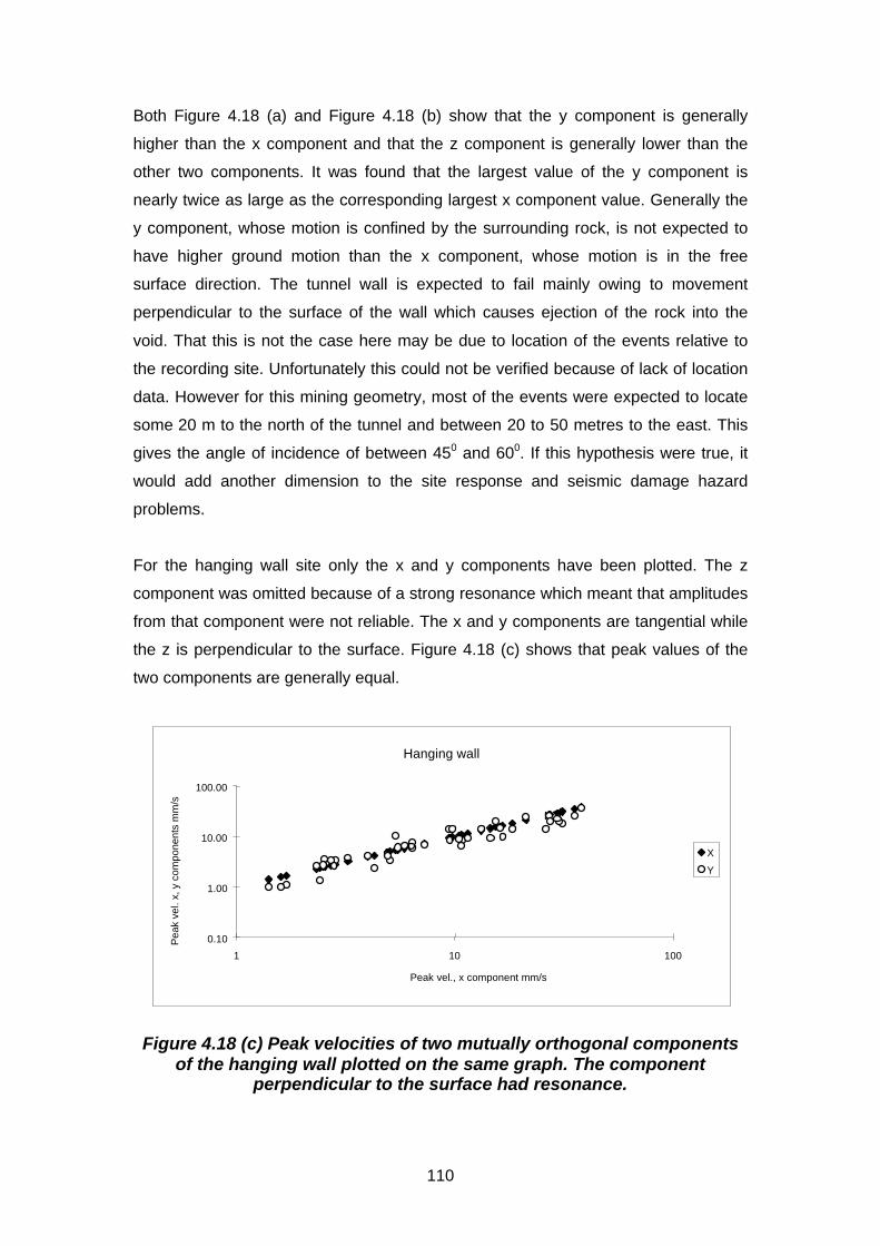
110
Both Figure 4.18 (a) and Figure 4.18 (b) show that the y component is generally
higher than the x component and that the z component is generally lower than the
other two components. It was found that the largest value of the y component is
nearly twice as large as the corresponding largest x component value. Generally the
y component, whose motion is confined by the surrounding rock, is not expected to
have higher ground motion than the x component, whose motion is in the free
surface direction. The tunnel wall is expected to fail mainly owing to movement
perpendicular to the surface of the wall which causes ejection of the rock into the
void. That this is not the case here may be due to location of the events relative to
the recording site. Unfortunately this could not be verified because of lack of location
data. However for this mining geometry, most of the events were expected to locate
some 20 m to the north of the tunnel and between 20 to 50 metres to the east. This
gives the angle of incidence of between 450 and 600. If this hypothesis were true, it
would add another dimension to the site response and seismic damage hazard
problems.
For the hanging wall site only the x and y components have been plotted. The z
component was omitted because of a strong resonance which meant that amplitudes
from that component were not reliable. The x and y components are tangential while
the z is perpendicular to the surface. Figure 4.18 (c) shows that peak values of the
two components are generally equal.
Hanging wall
0.10
1.00
10.00
100.00
1 10 100
Peak vel., x component mm/s
Pea
k ve
l. x,
y c
ompo
nent
s m
m/s
X
Y
Figure 4.18 (c) Peak velocities of two mutually orthogonal componentsof the hanging wall plotted on the same graph. The component
perpendicular to the surface had resonance.

111
Furthermore, a comparison between the western and eastern sidewalls was done.
Peak velocities of events common to both walls were plotted on the same graph.
Channel by channel plots was done. These graphs are shown in Figure 4.19 (a),
Figure 4.19 (b) and Figure 4.19 (c).
X component
1
10
100
1 10 100
Peak vel., Ewal (mm/s)
Pea
k ve
l., E
wal
l, W
wal
l (m
m/s
)
Ewall
Wwall
Figure 4.19 (a) Peak velocities of events common to eastern and westernwalls recorded perpendicular (x component) to the walls.
Y component
1.00
10.00
100.00
1.00 10.00 100.00
Peak vel. , Ewall (mm/s)
Pea
k ve
l., E
wal
l, W
wal
l (m
m/s
)
Ewall
Wwall
Figure 4.19 (b) Peak velocities of events common to eastern and westernwalls recorded tangential (y component) to the walls
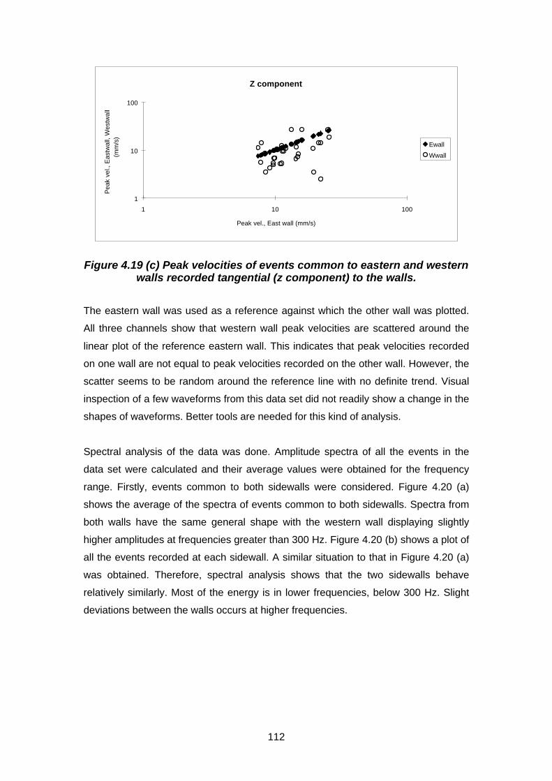
112
Z component
1
10
100
1 10 100
Peak vel., East wall (mm/s)
Pea
k ve
l., E
astw
all,
Wes
twal
l (m
m/s
)
Ewall
Wwall
Figure 4.19 (c) Peak velocities of events common to eastern and westernwalls recorded tangential (z component) to the walls.
The eastern wall was used as a reference against which the other wall was plotted.
All three channels show that western wall peak velocities are scattered around the
linear plot of the reference eastern wall. This indicates that peak velocities recorded
on one wall are not equal to peak velocities recorded on the other wall. However, the
scatter seems to be random around the reference line with no definite trend. Visual
inspection of a few waveforms from this data set did not readily show a change in the
shapes of waveforms. Better tools are needed for this kind of analysis.
Spectral analysis of the data was done. Amplitude spectra of all the events in the
data set were calculated and their average values were obtained for the frequency
range. Firstly, events common to both sidewalls were considered. Figure 4.20 (a)
shows the average of the spectra of events common to both sidewalls. Spectra from
both walls have the same general shape with the western wall displaying slightly
higher amplitudes at frequencies greater than 300 Hz. Figure 4.20 (b) shows a plot of
all the events recorded at each sidewall. A similar situation to that in Figure 4.20 (a)
was obtained. Therefore, spectral analysis shows that the two sidewalls behave
relatively similarly. Most of the energy is in lower frequencies, below 300 Hz. Slight
deviations between the walls occurs at higher frequencies.

113
Common events
-1
-0.8
-0.6
-0.4
-0.2
0
0.2
0.4
0.6
0.8
1
47 141 235 329 423 518 612 706 800 894 988
Frequency (Hz)
Log 1
0 V
el. S
pect
rum
Ewall
Wwall
Figure 4.20 (a) Log10 average velocity spectra of events from the easternwall (solid line) and events from the western wall (dashed line). Only
events common to both walls were considered
All events
-1
-0.8
-0.6
-0.4
-0.2
0
0.2
0.4
0.6
0.8
1
47 141 235 329 423 518 612 706 800 894 988
Frequeny (Hz)
Log 1
0 V
el. s
pect
rum
Ewall
Wwall
Figure 4.20 (b) Log10 average velocity spectra of events from the easternwall (solid line) and events from the western wall (dashed line). All
events recorded at the walls were considered.
114
4.3.5 Conclusions and discussions
Peak velocities may be affected by the position of the event source relative to the
wall of the excavation. This directional dependence means that some parts of the
excavation may be more hazardous than others. Spectral analysis shows that the
both sidewalls of the tunnel behaved relatively similarly. However this will depend
mostly on the frequency content of the incident wave as well as on the direction
(position) of the source relative to the tunnel. A complete analysis of these
phenomena requires location data and a reference geophone embedded in the solid
rock.
5 New interpretation techniques and
developments
5.1 Rock mass behaviour under seismic loading in a
deep mine environment
5.1.1 Summary
The dynamic behaviour of the rock mass surrounding a stope has been studied in a
deep South African gold mine. The three-dimensional seismic network installed at
Western Deep Levels East Mine, affords a unique opportunity to examine the change
in the wave front close to an underground opening. A set of three-component
sensors installed in a borehole above the panel reveals the development of surface
waves as the wave front reaches the excavation. An array of vertical component
sensors installed on the hangingwall of the excavation provides a two-dimensional
image of site effects. The collected data did not include damaging seismic events.
Quantitative analysis of the data, however, enables phenomena to be recognised,
which could lead to damage.

115
In the vicinity of the excavation, the energy of the seismic signal is generally
transformed from high frequency to low frequency. A strong structural effect is
expressed by the well-developed coda of low frequency (at 40 Hz and around 60-
70 Hz) at the skin of the hangingwall. The strong low frequency component is not
present on records from stations located in solid rock.
A seismic source with relatively high corner frequency (150 Hz-200 Hz) usually
excites several modes from 30 Hz to 110 Hz in the hangingwall of the excavation.
The seismic sources with low corner frequency (30 Hz-50 Hz) do not always excite
higher modes of vibration in the structure. This implies that the rock mass around the
excavation is a complex medium, and should be studied using the multi-degree-of-
freedom model.
The site effect is defined as a change in signal properties from station to station
located in the hangingwall. The site effect usually produces strong resonance around
160 Hz and in a frequency range from 200 Hz to 300 Hz. This effect causes the
relative displacement between blocks surrounding the excavation. Time domain
analysis of the seismograms, using the transfer function technique, confirms site
effect resonance.
Apart from the structural and site effects, the distance of seismic source from the
excavation also has a significant influence on vibration.
5.1.2 Introduction
One of the most important problems encountered in engineering seismology is the
prediction of ground motion parameters at the site of interest. The classical approach
is to evaluate peak ground velocity as a function of distance between source and
station (R) and magnitude of seismic event (M) (Kaiser, 1993). In this type of
equation, the stress drop of the seismic event (∆σ) often replaces the magnitude as
stress drop relates directly to peak ground velocity (McGarr et al., 1981). No damage
is expected when peak ground velocity is small. However, records of falls of ground
collected at East Rand Proprietary Mine show that peak ground velocities as small as
0,005 m/s can cause damage (Cichowicz, 1995).
116
The estimations show that most damage occurred at peak ground velocity smaller
than 1 m/s. Similar low values of damaging peak ground velocity were estimated by
Butler and Van Aswegen (1993). These estimations came from the Vmax (∆σ, R)
relationship, which is only applicable for far field seismic stations located in solid
rock. However, the presence of the free surface, fractured rock surrounding the
excavations, and the geometry of the excavation influence the ground motion at the
excavation wall. These phenomena can cause unusual amplification of ground
motion parameters at the site (Durrheim et al., 1996).
The following procedures were applied to analysis of the seismic data:
• study of the anatomy of the seismograms to identify body and surface waves
• three-dimensional image of ground motion
• filtration of the velocity signal with a band pass Butterworth filter
• spectral analysis
• interpretation of surface wave
• one-dimensional and two-dimensional resonance
• mode analysis
5.1.3 Three-dimensional image of ground motion
The three-dimensional seismic network installed at Western Deep Levels, East Mine,
93 E 4 panel, gives the unique opportunity to examine the change in the wave form
close to an underground opening. Standard analysis of wave propagation was used
to explain the effects experienced by waves as they propagate through a section of a
structure.
Four three-component sets of geophones were installed in a borehole (Figure 4.5).
The deepest set of three sensors (station A) used in analysis was installed at a depth
of 6,5 m. The shallowest set (station D) was installed at a depth of 0,5 m. Stations B
and C were located between station A and station D, 2 m apart. The amplitude of the
ground motion is expressed in units of mm/s. Another array of five vertical
geophones was installed on the skin of the hangingwall in the vicinity of the borehole
mouth. Additionally, one vertical geophone was installed on the footwall. The sensors
on the skin of the hangingwall were connected to the Ground Motion Monitor (Milev
et al., 1998).

117
After adjustment of time and amplitude scales of both systems, it was possible to the
compare waveforms recorded in the vertical borehole array, with the corresponding
waveforms recorded at the skin of the excavation.
Data from the vertical array (Figure 5.1) shows records with well-developed groups of
P- and S-waves. The group of body waves is followed by low frequency surface
waves.
0.02 0.04 0.06 0.08 0.1 0.12-1.5
-1
-0.5
0
0.5
1
1.5
Time [s]
Station A
0.02 0.04 0.06 0.08 0.1 0.12-1.5
-1
-0.5
0
0.5
1
1.5
Time [s]
Station B
0.02 0.04 0.06 0.08 0.1 0.12-1.5
-1
-0.5
0
0.5
1
1.5
Time [s]
Station C
0.02 0.04 0.06 0.08 0.1 0.12-1.5
-1
-0.5
0
0.5
1
1.5
Time [s]
Station D
Figure 5.1. Seismograms recorded by the Portable Seismic System(borehole array, vertical channels). Stations A, B, C and D are located
from the top to the bottom.
There are several points in time where the amplitude of the group of body waves
shows a sharp change in phase - these points are associated with new arrivals. This
indicates that the structure is rather complex and also that the seismic events are
located close to a three-dimensional array. The sites A and B have almost identical
waveforms. A straight extrapolation from the waveform of station B to the waveform
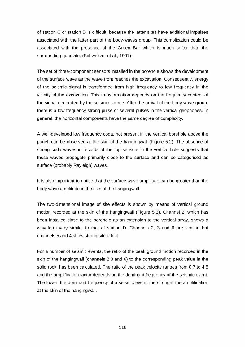
118
of station C or station D is difficult, because the latter sites have additional impulses
associated with the latter part of the body-waves group. This complication could be
associated with the presence of the Green Bar which is much softer than the
surrounding quartzite. (Schweitzer et al., 1997).
The set of three-component sensors installed in the borehole shows the development
of the surface wave as the wave front reaches the excavation. Consequently, energy
of the seismic signal is transformed from high frequency to low frequency in the
vicinity of the excavation. This transformation depends on the frequency content of
the signal generated by the seismic source. After the arrival of the body wave group,
there is a low frequency strong pulse or several pulses in the vertical geophones. In
general, the horizontal components have the same degree of complexity.
A well-developed low frequency coda, not present in the vertical borehole above the
panel, can be observed at the skin of the hangingwall (Figure 5.2). The absence of
strong coda waves in records of the top sensors in the vertical hole suggests that
these waves propagate primarily close to the surface and can be categorised as
surface (probably Rayleigh) waves.
It is also important to notice that the surface wave amplitude can be greater than the
body wave amplitude in the skin of the hangingwall.
The two-dimensional image of site effects is shown by means of vertical ground
motion recorded at the skin of the hangingwall (Figure 5.3). Channel 2, which has
been installed close to the borehole as an extension to the vertical array, shows a
waveform very similar to that of station D. Channels 2, 3 and 6 are similar, but
channels 5 and 4 show strong site effect.
For a number of seismic events, the ratio of the peak ground motion recorded in the
skin of the hangingwall (channels 2,3 and 6) to the corresponding peak value in the
solid rock, has been calculated. The ratio of the peak velocity ranges from 0,7 to 4,5
and the amplification factor depends on the dominant frequency of the seismic event.
The lower, the dominant frequency of a seismic event, the stronger the amplification
at the skin of the hangingwall.
119
0.02 0.04 0.06 0.08 0.1 0.12-3
-2
-1
0
1
2
3
Time [s]
Channel 2
0.02 0.04 0.06 0.08 0.1 0.12-3
-2
-1
0
1
2
3
Time [s]
Channel 3
0.02 0.04 0.06 0.08 0.1 0.12-3
-2
-1
0
1
2
3
Time [s]
Channel 4
0.02 0.04 0.06 0.08 0.1 0.12-3
-2
-1
0
1
2
3
Time [s]
Channel 5
0.02 0.04 0.06 0.08 0.1 0.12-3
-2
-1
0
1
2
3
Time [s]
Channel 6
0.02 0.04 0.06 0.08 0.1 0.12-3
-2
-1
0
1
2
3
Time [s]
Channel 7
Figure 5.2 Seismograms recorded by the Ground Motion Monitor(surface array, vertical channels). Channels 2, 3, 4, 5 and 6 are located
on the skin of the hangingwall and channel 7 is on the footwall.

120
5.1.4 Spectral analysis of the three dimensional ground
motion
Spectral analysis was carried out on all the records. The objective of this analysis was to
identify common features responsible for the structural effect and the site effect in the
frequency domain.
Data from the borehole array were used to identify the dominant frequency of the
seismic source. This task, which is performed routinely in the study of seismic source
parameters, gives uncertain results. At station A, the vertical component of the
seismograms is controlled by source properties and by structural effects. Therefore, the
group of body waves recorded by the horizontal components was used to calculate the
corner frequency of the seismic source (see the second column of Table 5.1).
Table 5.1
Spectral peaks from the vertical borehole array (Portable Seismic Systemdata). The peaks without letters indicate that amplification was observed at
all geophones, letter D or C indicates that the peak was observed only atthat particular geophone.
Event
Number fo [Hz] Body Wave Peaks [Hz]
Surface Wave
Peaks [Hz]
5243 120-180 105 (200 280 400)C 40 70
5361 200 70-80 (220 400)C 45 60
5384 120-200 60 40 70
5509 200 70-80 140D (180 280 350)C 50 80D 90C
5634 100-200 70-80 140D (180 280 350)C 45 80D 90C
5635 200-350 70-80 140D (200 280 350)C 40 60
Spectra of the vertical components of the borehole array were obtained separately for
the body wave group and the surface waves. Table 5.1 shows the spectral peak for both
groups. The peaks without letters indicate that amplification was observed at all

121
geophones, letter D or C indicates the peak was observed only at that particular
geophone.
The body wave group has a systematic peak around 70 Hz, which does not relate to the
corner frequency of the seismic source. At station C, spectra have several systematic
peaks, which could be related to the interaction of the seismic wave with the Green Bar.
Station D often has amplification at 140 Hz.
The image given by spectra of the surface wave clearly indicates that there are usually
two strong peaks at 40 Hz and 60-70 Hz, and obviously the surface wave carries
information about structure.
The amplitude of the surface waves recorded by the vertical components increased from
station A to station D. The surface waves amplitudes at station A are half those of station
D. In addition, there is a significant difference between the amplitude spectra of station A
and station D. On average, the peaks of surface spectra are about 6 to 11 times stronger
at station D than the peaks at station A. Figure 5.3, shows a systematic peak increase of
the 70-80 Hz as the geophones approaching close to the skin of the excavation.

122
Figure 5.3 Amplitude spectra of body wave group for events recorded bythe borehole array. The records from sites A and B are marked by a solid
lines; record from station C is marked with dashed-dot line and record fromstation D is marked by a dotted line.
The array installed in the hangingwall and footwall is used to study the spectral peaks
associated with structural and site effects. Table 5.2 shows different dominant
frequencies for a number of seismic events observed in channels 2, 3 and 6, and that
are not present at station A in solid rock. The peaks are caused by a structural effect, as
they are observed at several points in the hangingwall. The prominent finding is that the
structure can produce several spectral peaks. Seismic events do not however excite all
possible resonance frequencies. Nevertheless, resonance at 30 Hz and 60 Hz is
observed most frequently. The location of seismic the events with respect to the position
of the stop is the second important feature (the first being structural properties), which
determines excitation of the selected resonance.

123
Table 5.2
Spectral peaks observed at the skin of the hangingwall channels 2, 3 and 6;the peaks are marked by the symbol “ * ”.
Event
number
Spectral Peak [Hz]
30 40 50 60 70 80 90 100 110 120
3 *
7 * * * *
14 * * *
25 * * * * *
26 *
37 * * * * * *
38 * * * *
42 * * * *
43 * * *
45 * * * *
48 * * *
59 * *
64 * * *
72 * * * *
75 *
83 *
88 * *
89 * * * *
Inspection of the spectral peaks shows that channels 4 and 5 have site effects in
addition to the structural effect. Channel 5 has a very strong resonance at 160 Hz for all
seismic events, however data from Table 5.2 do not show such pronounced resonance.
Once again, this indicates that the location of the seismic event is the crucial parameter
determining excitation of resonant frequency modes. Channel 4 shows a very strong
resonance over a broad range of frequencies from 160 Hz to 300 Hz.
124
The records of the geophone on the footwall (channel 7) in some cases have relatively
strong surface waves, which were not observed at the hangingwall sites. In another
case, records of the footwall geophone show a very strong signal around 300 Hz and
surface wave was not observed.
5.1.5 Structural effect
Almost all records from the hangingwall, the footwall, and the borehole show surface
waves. The pulses on the seismograms were classified as surface (Rayleigh) waves
when the following features were present:
• arrival after the S-wave,
• frequency contents much lower than body waves,
• decrease in amplitude with distance from the free surface of the underground
excavation.
A number of different researchers have confirmed that the dominant frequency of the
Rayleigh wave is strongly dependent on the variation of shear wave velocity with depth
at the site (Murphy and Shah, 1988). The characteristic dominant frequency at the site
can be approximated by the following equation:
HVf 3.2/= (5.1)
where: V is the average shear wave velocity and H denotes the depth to the first
significant discontinuity. The dominant frequencies of surface pulses wave 40 Hz, 70 Hz
and 90 Hz. Thus possible causes of the generation of these waves are layers of
30 m (40 Hz), 20 m (70 Hz) or 14 m (90 Hz) in thickness. The dominant frequency and
location of the seismic source determines which layer is excited.
There is a two metres thick layer of Green Bar at 1,0 to 1,8 above the free surface of the
excavation. This layer could be responsible for the peak in the spectrum around 350-
400 Hz, if it was present everywhere. However, this peak is not strong.

125
The presence of several Rayleigh wavelets in the seismograms could be interpreted in
terms of the existence of a complex structure around the stope. The results of
experimental techniques (Daehnke et al., 1997) and numerical modelling (Hildyard et al.,
1995) were used to explain the wave interaction with the stope. Three models were
investigated: (1) a stope situated in a homogeneous medium, (2) a stope surrounded by
fracture softened material, where the interface between the softened and bulk material is
bonded, (3) a stope situated within a softened material, with a non-cohesive material
interface. The results from the three models were generalised as: (i) Rayleigh wave is
well developed in the hanging – and footwall. (ii) Rayleigh waves are able to propagate
along the hangingwall and footwall surface, (iii) The non-cohesive parting plane traps
energy within the hangingwall and footwall beams in the form of reflected shear waves.
In the third experiment the coda wave was much stronger than in the second
experiment.
There is an alternative explanation for the surface wave. Lateral changes in the shear
wave velocity could lead to the formation of a Rayleigh wave that contains delayed
surface waves that reach the seismic station indirectly. The vertical discontinuity could
gives rise to the development of surface waves, which then propagate back and forth
within the lateral structure. The complicated structure of the recorded Rayleigh waves
makes it impossible to identify vertical discontinuities using a small number of recordings
(Meier at al., 1998).
5.1.6 Site Effect – Microzonation
The seismic array in the hangingwall was used to study the site effect. The prominent
features of records or spectra unique to each record from the hangingwall are called the
site effect. Channels 4 and 5 show strong site effects for all seismograms. Channel 5
has strong resonance at 160 Hz (about 20 m wavelength). Channel 4 usually has
several peaks around 160 Hz and 300 Hz. At the channel number 3, an 160 Hz peak
can be observed but it is very small.

126
A band pass Butterworth filter (120 Hz-250 Hz) was applied to data from stations 4 and 5
to study the resonance frequency signal in the time domain. At station 4 the filtered
signal is strong at the arrival of the SV group (only the vertical component is available)
and quickly decays. Usually the resonance signal is not present in the coda. At station 5
the selected signal is distributed across the entire seismogram and its amplitude is
smaller than the one recorded at station 4.
The site effect can be explained by introducing a local contrast in medium properties: the
contrast between the Green Bar and the quartzite, or the difference in fracture intensity
of the rock around the excavation. The site effect is not observed at channel 2 and
channel 6 indicating that the width of the inhomogeneity is less than two metres. The
length is not well defined, as there is no other station to the right side of geophone 5.
A one-dimensional resonant frequency (fh) model is commonly applied to estimate the
thickness of the layer causing resonance (H = Vs / 4 fh). However, a numerical study
leads to the conclusion that the two-dimensional resonant frequency and amplification
values differ substantially from their one-dimensional estimate. Bard and Bouchon
(1985) showed that the transfer function for different sites at the surface of a sine-
shaped valley exhibits specific resonance patterns, with the following characteristics:
• the frequency of the resonance peak is the same at each location within the inclusion
regardless of local thickness
• the two-dimensional resonance is controlled by the shape ratio (thickness to half-
length ratio) and the impedance contrast insignificant
• the corresponding amplification is the largest in the inclusion centre, and decays
toward the edges
The observed pattern of resonance peaks and the motion duration of the resonance
frequencies indicate that geophone 5 is in the centre of the inhomogeneity, geophone 4
is off centre and geophone 3 is at the edge.
The one-dimensional resonance at 160 Hz gives a layer thickness of about 4,7 m (for
VS = 3000 m/s). However this thickness has to be rejected as geophone 2 and 6 do not
show similar resonance frequencies.
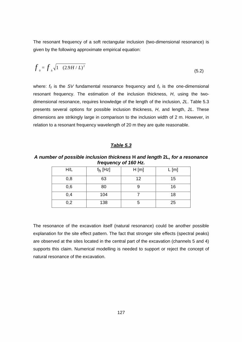
127
The resonant frequency of a soft rectangular inclusion (two-dimensional resonance) is
given by the following approximate empirical equation:
0
21 2 9f fh
H L= + ( . / )(5.2)
where: f0 is the SV fundamental resonance frequency and fh is the one-dimensional
resonant frequency. The estimation of the inclusion thickness, H, using the two-
dimensional resonance, requires knowledge of the length of the inclusion, 2L. Table 5.3
presents several options for possible inclusion thickness, H, and length, 2L. These
dimensions are strikingly large in comparison to the inclusion width of 2 m. However, in
relation to a resonant frequency wavelength of 20 m they are quite reasonable.
Table 5.3
A number of possible inclusion thickness H and length 2L, for a resonancefrequency of 160 Hz.
H/L fh [Hz] H [m] L [m]
0,8 63 12 15
0,6 80 9 16
0,4 104 7 18
0,2 138 5 25
The resonance of the excavation itself (natural resonance) could be another possible
explanation for the site effect pattern. The fact that stronger site effects (spectral peaks)
are observed at the sites located in the central part of the excavation (channels 5 and 4)
supports this claim. Numerical modelling is needed to support or reject the concept of
natural resonance of the excavation.

128
5.1.7 Multi-degree-of-freedom model in time and
frequency domains
A method for the time-domain identification of linear multi-degree of freedom structural
dynamic systems was outlined by Cichowicz and Durrheim, (1997). Seismic records of a
single input and single output are sufficient to determine the transfer function between
seismic sensors installed in the solid rock and at the skin of the hangingwall. The
transfer function is parameterised as a series of damped oscillators.
The transfer function is obtained in a time domain inversion process. This approach has
the additional benefit of being able to observe how the excavation effect and the site
effect develop during ground motion caused by a seismic event.
Data from the borehole array shows that the transfer function has at least three different
phases. Two phases are observed in the shear wave group and the third phase is
associated with surface waves. This indicates that the group of body waves has a very
complex composition. Therefore it is difficult to model the whole seismogram with one
transfer function. A model of the transfer function obtained at the end of a seismogram
matches the output reasonably well, however to get the perfect match it is necessary to
use a separate transfer function for each of the three intervals of the seismogram. The
good match in the time domain indicates that the spectral peaks can be modelled using
damped oscillators.
Data from the hangingwall array are modelled reasonably well with one transfer function.
The transfer function from the end of the seismogram matches the whole record. This
indicates that the interaction between blocks in the hangingwall can be modelled using
several damped oscillators. Figure 5.4 shows the sum of three modal responses
calculated at the time 0,105 s (solid line). The model of ground motion correlates well
with the real one. (channel 5 - dashed line). The modal frequencies are 225 Hz, 413 Hz
and 431 Hz and respective damping ratios are 0,258; 0,075 and 0,462.

129
Figure 5.4 The sum of three modal responses calculated at the time 0,105 s(solid line); the match with the real ground motion is very good (channel 5 -
dashed line).
Figure 5.5 shows the spectra of the real output (channel 5 is marked by a solid line) and
the calculated one (dashed line). Third curve is the transfer function in the frequency
domain between channel 5 and channel 6. Resonance at 160 Hz is observed but is very
weak. The transfer function does not include 160 Hz resonance.

130
Figure 5.5 Observed (solid line) and calculated (dashed line) spectra forchannel 5. The third curve is the transfer function in the frequency domain
between channel 6 and channel 5.

131
5.1.8 Conclusions
A comparison of the records from the borehole array with the records from the skin of
the hangingwall quantifies the influence of an underground excavation on the ground
motion parameters. Seismic sensors placed in a borehole provide information on the
seismic source and structural effects. The array of sensors installed at the skin of the
hangingwall provides information about the excavation effect and the site effect.
Structural Effect• The seismic signal is amplified 2-4 times at the skin of the hangingwall. The spectral
peak associated with structural resonance can be up to 10 times stronger than the
signal from solid rock.
• Apart from the structural effect and site effect, the distance of the seismic source
from the excavation has a significant influence on the vibration.
• The amplitude of the low frequency signal of the surface wave can be greater than
that of the body wave. This low frequency signal is created by the structural effect. A
low velocity layer around the excavation with a non-cohesive material interface or
vertical discontinuities around the excavation can be responsible for the creation of
the strong low frequency signal.
• The broad spectrum of possible modal resonance (30 Hz, 50 Hz, 60 Hz, 80 Hz and
110 Hz) indicates the structures surrounding Western Deep Levels are complex.
Site effect• The site effect is visible as a strong amplification of selected frequencies at channel
4, and 5 on the surface.
• The observed pattern in time and frequency domain suggests that a two-dimensional
inclusion is responsible for the site effects. The amplification value associated with a
two-dimensional inclusion is extremely large. As a consequence, these values must
be taken into account during the assessment of the local seismic hazard.
• The resonance of the excavation itself (natural resonance) could be another possible
explanation for the site effect pattern. The fact that stronger site effects (spectral
peaks) are observed at the sites located in the central part of the excavation
(channels 5 and 4) supports this claim.

132
5.2 Monitoring falls of ground with Modified Ground
Motion Monitor
The management of Lonrho Platinum Mine requested CSIR Mining Technology to
developed a method of determining the exact time and location of falls of ground in the
mining panels. There was the opinion that most of the falls of ground occurred during the
blasting time. A ground motion monitor was modified to fulfil this task.
In collaboration with GAP 416, and M & M Systems, the standard 5 m cable between
each geophone and recording box was replaced with 100 m bell wire thin enough to be
broken by an average sized fall of ground. This wire was then attached to the
hangingwall between the support units. The hangingwall of a potentially hazardous panel
was then banded as is shown in Figure 5.6.
BB
FACE
G1
G2
G3
FOG6 May '98
17:33:05 to 52
OLD FOG
Gul
ly
Figure 5.6 Sketch of the geophones and wire deployment for monitoring fallof grounds (FOG) at Lonrho Eastern Plats belt 2.

133
Figure 5.7 illustrates two consecutive seismograms where channel 3 was disconnected
after the fall of ground had cut the circuit. The accuracy of this case is 47 s, or the time
interval between these two consecutive events.
Lonrho Eastern Platinum Mine6 May '98
-60
-40
-20
0
20
40
60
0 200 400 600 800 1000
Counts
Vel
oci
ty [
mm
/s]
G1 G2 G3
17:33:05 17:33:52
Figure 5.7 Two consecutive seismograms before and after the fall ofground on 6 May ’98, recorded at 6 E 1 down-dip Lonrho Eastern Plats
belt 2
The development of maximum velocities in the progression to the fall of ground is shown
in Figure 5.8. It can be seen that the fall of ground occurred at maximum velocities in the
range of 50 to 60 mm/s.

134
Lonrho Eastern Platinum Mine
0
10
20
30
40
50
60
17:24:00 17:25:26 17:26:53 17:28:19 17:29:46 17:31:12 17:32:38 17:34:05 17:35:31
6 May '98 Time [min]
PP
V [
mm
/s]
G1 G2 G3 FOG6 May '98
17:33:05 to 52
Figure 5.8 Maximum velocities as a function of time shortly before the fallof ground on 6 May ’98.
A few moments later a second fall of ground was monitored in a neighbouring panel. In
both cases the falls of ground occurred during blasting.
The new modification to the Ground Motion Monitor successfully fulfilled the requirement
of monitoring the time of fall of ground.
5.3 Single-block rockburst model
Rockburst-resistant support is currently designed on the basis of an ejection velocity,
usually of the order of 3 m/s. The mechanisms of ejection are still a matter for debate. In
even the most severe rockburst, there is always rock that has not been ejected. In most
minor rockbursts only isolated blocks come out of the hangingwall. Figure 5.9 shows a
model of a single-block rockburst, or shake-out.

135
σh
σhm(g+a)
-300
-200
-100
0
100
200
300
400
500
600
0 10 20 30 40 50 60 70 80 90
Ground velocity, mm/s
country & block-country
Parting
Figure 5.9 Sketch of a single-block rockburst. In this model, the totalamount of damage, or relative slip, amounted to 9 mm.
The essence of this model is that damage results from the inability of blocks to move up
when the rock mass moves up. In this model, horizontal stress and vertical acceleration
control damage.
1. Horizontal stress, quasi-static and dynamic, holds the block in place even during
upward acceleration through friction. The dynamic stress can be estimated from
the ground motion.
2. The effective weight, or downward force, of the block is increased as the
adjacent rock mass is accelerated upwards.
Relative motion and damage occur when the vertical downward forces exceed the
vertical upward forces on the block. Damage can accumulate over successive cycles of
ground motion.
In addition, damage can possibly be caused by high horizontal stresses, especially when
a weak parting is in the immediate hangingwall.
136
Given the existence of blocks surrounded by fracture planes with known strength, the
accuracy of this model depends mostly on deriving good estimates of dynamic stress
from seismograms. Rayleigh waves and vertically moving P-waves have been assumed.
In the second half of 1998, further models were considered and applied to existing data.
6 Conclusions and Recommendations
The first enabling output involves comprehensive investigations of at least four rockburst
accident sites. The investigation by a team of specialists typically encompassed an
assessment of the source and damage mechanisms, layout, and support performance.
In addition it was decided to include less detailed investigations of other rockburst sites.
• The most common source mechanism of a causative seismic event is slip on
either a dyke contact or a fault. In some cases the seismic data coupled with the
extent, nature and location of the damage allowed the identification of the source
mechanism with a high degree of accuracy.
• Other identified source mechanisms include remnant pillar failure, stabilising
pillar foundation failure and face bursting.
• The most common damage mechanism resulting from seismic activity is
predictably, collapse and shakedown of hangingwall. Other mechanisms are
tunnel wall damage, footwall heave and face rock ejection.
• Many factors affected the severity of damage. Mine layout factors included poor
remnant shape, poor pillar design, breast-on face orientation when approaching
geological features and excessive leads or lags between panels. Incorrect input
parameters, such as k-ratios, when modelling also resulted in poor layouts.
Tunnels positioned in fault loss zones sustained serious damage in some cases.
Inappropriate and poorly designed support in tunnels, gullies and stopes and in
some cases sub-standard application of the support in these excavations also
played a role in determining the severity of the damage sustained.
• Assumptions regarding the stress field affecting a particular mine are probably
invalid in many cases. An improved knowledge of the stress field would assist
significantly with mine layout (numerical modelling) and both local and regional
137
support planning. It is recommended that mines make use of a database of
stress measurements that has recently been established and in some cases
additional stress measurements may be necessary where anomalous situations
are evident or anticipated.
• The degree of corrosion of tunnel support can have a significant effect on the
extent and severity of damage resulting from a seismic event. Where tunnels are
needed for extended periods, and where seismic activity is likely, areas where
support may be compromised must be identified and rehabilitated.
• The depth of the unstable zone surrounding tunnels needs to be estimated. This
determines the length and spacing of tendon support.
• The siting of tunnels and crosscuts in fault loss zones where extensive mining of
nearby reef is planned should be avoided.
• Cementitious packs, designed to yield at loads lower than that required to induce
damage in the gully sidewall, have been seen to perform well under dynamic
loading. In one case a direct comparison with timber packs could be made.
• The stability of remnant pillars depends largely on the shape and the width:
height ratio. The latter may be affected by local geology and by reef geometry. A
triangular shape, as opposed to L-shaped or narrow rectangular remnants, which
are particularly troublesome, is recommended.
• Backfill can be shown to have a significant regional and local support benefit in
some areas particularly on the Far West Rand. The positive effect that backfill
has on gully and stope conditions has been observed.
The second enabling output involved the measurement and analysis of the dynamic
response of the rock surrounding excavations to seismic shaking. The measurement
was be done by means of ground motion monitors in stopes and tunnels. Techniques
were developed or adapted for analysing the data. In addition a controlled seismic
source (simulated rockburst) was carried out to augment the findings. The influence of
support elements and the integrity of the excavation skin was also assessed.

138
Controlled seismic source experiment
• The distance of the blast holes from the tunnel wall ensured that no gas pressure
was involved in damaging the wall of the tunnel. The damage resulted from the
interaction of shock wave with the tunnel, similar to what would happen in a
rockburst. Petroscope probes and ground penetrating radar scans confirmed the
development of new fractures close to and parallel to the damaged tunnel wall.
• Two areas of damage have been identified on the blasting wall:
Ø area with high intensity damage: ejection velocity at 3,3 m/s was
recorded by an accelerometer ejected with a block of rock
Ø area with low intensity damage: ejection velocity at 1,6 m/s was
recorded by an accelerometer left over the blasting wall
• High speed camera shots revealed rock fragments being ejected from the wall at
velocities in the range of 0,7 m to 2,5 m per second. The measurements were
taken in the area of low intensity damage.
• The maximum velocity recorded in the solid rock close to the blast was compared
to the velocities recorded on the blasting wall. The ratio of 2,2 times, between the
solid and the area with high intensity damage and ratio of 1,3 times between the
solid and the area with low intensity damage were found.
• Peak particle velocities recorded on the blasting wall attenuate exponentially with
the distance. The velocities measured at distance of 30 m from the blast where at
about 20 times less than the velocities measured at 6 m from the blast. The
attenuation of the velocities obtained from the calibration blast have similar trend.
• The Vaal River Operations regional seismic network recorded the simulated
rockburst. The local magnitude was estimated as ML = 1,3. Further use of the
simulated rockburst for scaling of mine tremors located in this region is
recommended.
• Peak particle velocities (PPV’s) were measured on the tunnel wall both before
and after the experimental blast. The PPV’s were as a result of normal mining
operations some 100 m from the site. The amplification of the PPV’s after the
blast were amplified some five, six times indicating the effect of the damage
caused to the rock surrounding the excavation.
• In frequency domain well defined amplification was obtain in the low frequency
band (0 – 100 Hz)

139
• The new fractures together with both natural bedding planes and “bow wave”
fractures formed during the development of the tunnel determined the shape of
blocks ejected from the wall at the time of the simulated rockburst.
• Tendon support of the tunnel had the effect of reducing the PPV’s and damage to
the wall in their immediate vicinity.
• It was found that the failure of the rock occurred predominantly on prominent
discontinuities such as bedding planes and fractures. Damage to a tunnel is
changed in the presence of discontinuities and this fact should be taken into
account when support is designed.
Dynamic behaviour of the rock around underground excavations
• The ground motion at points on the skin of a stope hangingwall was found to be
some four to ten times larger than at a point 6,5 m into the hanging wall. Coda
waves were also more developed on the skin. Measurements at 0,5 m, 2,5 m
and 4,5 m showed intermediate behavior. It was suggested that the fracture zone
acting as a wave-guide causes the enhanced levels of ground motion and that
multiple scattering causes the prolonged duration of motion.
• Ground motion on the abutment side of a fault in the hangingwall was much
lower than the ground motion on the other side.
• The results from velocity analysis have indicated that the time delays observed
between pairs of geophone sites exceeded the travel time for P- and S-waves, in
solid rock indicating lower wave velocities. These lower velocities are expected,
given the high degree of fracturing near the skin of the stope. It is expected that
this will give insight into the mechanisms of energy trapping. It will also assist in
estimating the effective stiffness of the fractured rock and, thereby, it’s dynamic
response.
• Two mechanisms of dynamic response have been defined: structural response,
defined as a common spectral behaviour at all surface seismograms; and local
site effect, defined by spectral peaks at one or two surface seismograms. The
spectral peaks interpreted as the structural response (40 Hz and 70 Hz for all
surface sites) could be associated with the presence of the Green Bar layer in
the quartzite, while the site effects observed at G4 and G5 would be more
dependent on the difference in the intensity of the local fractures in the vicinity of
140
the geophones. However, this interpretation is too broad and numerical modelling
is required to provide insights into the actual mechanism of dynamic behaviour of
the hangingwall.
• The results obtained for the dynamic response of the site, including both the
structural response and the local site effect, can be related to the existing support
methodology. The normalised load-deformation curve, presently used as a
support design criterion, could be modified by the dynamic response spectrum in
order to provide additional design information.
7 References
Aki, K. and Richards, P. G., 1980. Quantitative seismology, Freeman, San Francisco.
Anon, 1988. An industry guide to methods of ameliorating the hazards of rockbursts and
rockfalls. Chamber of Mines Research Organisation. Chamber of Mines of South Africa.
Bard, P. and Bouchon, M., 1985. The two-dimensional resonance of sediment-filled
valleys, Bull. Seism. Soc. of Am., Vol. 75, pp. 519-541.
Butler, A. G. and Van Aswegen, G., 1993. Ground velocity relationship based on a
large sample of underground measurements in two South African mining regions, In: R.
P. Young (Editor), Rockbursts and Seismicity in Mines, Kingston, Canada, pp. 41-51.
Cichowicz, A., 1995. Develop a more reliable means of assessing safety risk due to
rockbursts and rockfalls as a managerial decision support technique Report for CSIR
Mining Technology, Johannesburg, South Africa.
Cichowicz, A. and Durrheim, R.J., 1997. The Site Response of the Tunnel Sidewall in
a Deep Gold Mine, Analysis in the Time Domain, In: R.G. Gurtunca and T.O. Hagan
(Editors), Proc. 1st Southern African Rock Eng. Symp. Johannesburg South Africa, pp.
56-61.

141
Daehnke A., 1998. Personal communication on the choice of blast parameters. CSIR
Mining Technology, July, 1998.
Daehnke, A., Rossmanith, H. B. and Kanashmirner R. E., 1996. Using dynamic
photoelasticity to evaluate the influence of parting planes on stress wave interaction with
stopes, Int. J. Num. and Analy. Methods in Geomech., 20 pp.101-107
Daehnke, A., L. M. Andersen, D. de Beer, E. Esterheinzen, F. J. Glisson, E. P. Jaku,
J. S. Kuijpers, A. V. Peake, P. Piper, G. B. Quaye, N Reddy, M. C. K. Roberts, J. K.
Shweitzer, R. D., Steward. 1998. Stope Face Support systems, SIMRAC Final Report
on Project Report GAP 330. Pretoria: Department of Minerals and Energy, 530p.
Drescher, K 1998. Classification of rock specimen uniaxial compressive strength,
Internal report, CSIR: Division of Mining Technology, Auckland Park 2006, S.A.
Durrheim, R.J., Kullmann, D. H., Stewart, R. D. and Grodner, M. 1996. Seismic
excitation of the rock mass surrounding an excavation in highly stressed ground. In M.
Aubertin, F. Hassani and H. Mitri (eds), Proc. 2nd North American Rock Mechanics
Symposium: 389-394. Rotterdam: Balkema.
Durrheim, R.J., Milev, A.M., Spottiswoode, S.M. & Vakalisa, B. 1997. Improvement of
worker safety through the investigation of the site response to rockbursts, SIMRAC Final
Project Report GAP 201. Pretoria: Department of Minerals and Energy, 530p.
Durrheim, R.J., Roberts, M.K.C., Haile, A.T., Hagan, T.O., Jager, A.J., Handley, M.F.,
Spottiswoode, S.M. & Ortlepp, W.D. 1998. Factors influencing the severity of rockburst
damage in South African gold mines, Journal of South African Institute for Mining &
Metallurgy Vol. 98, No.2. 53-57.
Durrheim, R. J., Jager, A. J. and G. York. 1998. Rock engineering aspects of the
rockburst at No. 11 shaft, Impala Platinum Mine, on 31 December 1997, Internal report,
CSIR: Division of Mining Technology, Auckland Park 2006, S.A.

142
Essrich, F. and Amidzic, D. 1999. Influence of backfill on seismicity in the West Rand
Region. To be published. 2nd Southern African Rock Engineering Symposium
(SARES99). Sept 1999. Johannesburg.
Finnie, G. J., 1998. Personal communication on the seismic parameters reported by
Vaal River Operations regional seismic network, Vaal Reef, 2162.
Grave, M. 1998. The extensometer results of the sidewall-monitoring of 53-54 crosscut
at Vaal Reefs No. 9 Shaft following a simulated rockburst, Internal report, CSIR: Division
of Mining Technology, Auckland Park 2006, S.A.
Grodner, M. 1998. GPR Results from the Vaal Reefs controlled blast site, Internal
report, CSIR: Division of Mining Technology, Auckland Park 2006, S.A.
Guler, G., G. B. Quaye, J. K. Shweitzer, M. Grodner, A. J. Jager, N. Reddy, L.
Andersen, and, A. Milev. 1998. A methodology for the definition of geotechnical areas
within the South African Gold and Platinum stoping horizons. SIMRAC, Final Project
Report GAP 416. Pretoria: Department of Minerals and Energy, 530p.
Hagan, T.O, Haile A. T., Spottiswoode S.M., Turner A.P. and Malan D.F. 1998.
Hartebeesfontein No. 4 Shaft: Rock Engineering Aspects of the Rockburst Accident on
the of 5th March 1998. Internal report, CSIR: Division of Mining Technology, Auckland
Park 2006, S.A.
Hagan, T. O., M. K. C. Roberts, A. T. Haile, A. Daehnke, N. Reddy, R. J. Durrheim,
and W. D. Ortlepp. 1997. Follow-up visit to the affected by the rockburst at Elandsrand
Gold Mine (Deelkraal Section) on 7 May 1997, Internal report, CSIR: Division of Mining
Technology, Auckland Park 2006, S.A.
Haile, A. T. 1998a. Strata control in tunnels and an evaluation of support units and
systems currently used with a view to improving the effectiveness of support, stability
and safety of tunnels, SIMRAC, Final Project Report GAP 335. Pretoria: Department of
Minerals and Energy, 135 p.

143
Haile, A. T. 1998b. Investigation of damage to 64 B West haulage at the Great Noligwa
Mine due to a seismic event of magnitude M = 3,7 on 21 August 1998, Internal report,
CSIR: Division of Mining Technology, Auckland Park 2006, S.A.
Haile, A.T., Turner A.P and Hagan T.O. 2000. Tunnel support design, implication from
a study of rockburst investigation. Proc. Of the World Tunnel Congress, Durban.
Hildyard, M. W., Daehnke, A. and Cundall, P. A., 1995. WAVE: A computer prog ram
for investigating elastodynamic issues in mining, Proc 35th U.S. Symp on Rock Mech.,
pp. 519-524.
Kaiser, A. G., 1993. Support of tunnels in burst-prons ground - Toward a rational design
methodology, In: R. P. Young (Editor), Rockbursts and Seismicity in Mines, Kingston,
Canada, pp. 13-29.
Kouzniak N. (1998). Personal communication on ‘Comparisons with the analytical
propagating source model’. University of Vienna, Austria.
Kouzniak N. and Rossmanith H.P. (1998). Supersonic detonation in rock mass -
Analytical solutions and validation of numerical models - Part 1 stress analysis. In print,
submitted to FRAGBLAST.
Lay, T. and Wallace, T.C. 1995. Modern Global Seismology, Academic Press, San
Diego, USA, p 49.
Le Bron, K. 1998. Determination of the average stress levels at the 53-54 crosscut at
Vaal Reefs No. 9 Shaft, Internal report, CSIR: Division of Mining Technology, Auckland
Park 2006, S.A.
Le Bron, K., A. T. Haile. 1998. Investigation of the influence of a support unit on the
stability of a tunnel in fractured rockmass as the seismic wave passes, Internal report,
CSIR: Division of Mining Technology, Auckland Park 2006, S.A.

144
Linkov, A. L. and Durrheim, R. J., 1998. Velocity amplification considered as a
phenomenon of elastic energy release due to softening, Proc of the 3rd conference of
mechanics of jointed and faulted rock, Ed H-P Rossmanith,, pp. 243-249
Lightfoot, N., Kullmann, D.H., Toper, A.Z., Stewart, R.D., Grodner, M., Janse van
Rensburg, A.L. & Longmore, P.J. 1996. Preconditioning to reduce the incidence of
face bursts in highly stressed faces. Mining Technology Division of CSIR, SIMRAC Final
Report, Project GAP 030.
McGarr, A., Green, R. W. E. and Spottiswoode, S. M., 1981. Strong ground motion of
mine tremors: some implications for near source ground parameters, Bull. Seism. Soc.
of Am., Vol. 71, pp. 295-319.
Meier, P. G., Malischewsky, P. G. and Neunhofer, H., 1998. Reflection and
transmission of surface waves at a vertical discontinuity and imaging of lateral
heterogeneity using reflected fundamental Rayleigh waves, Bull. Seism. Soc. of Am.,
Vol. 87, pp. 1648-1661.
Milev, A. M., Spottiswoode, S. M. and Stewart, R. D., 1998. Dynamic response of the
rock surrounding deep level mining excavations, Proc. 9th ISRM, Paris’99, submitted.
Murphy, J. R. and Shah, H. K., 1988. An analysis of the effects of site geology on the
characteristics of near-field Rayleigh waves, Bull. Seism. Soc. of Am. Vol. 78, pp. 64-82.
Napier. J, F. Malan, E. Sellers, A. Daehnke, M. W. Hilyard, T. Dede, and, K and J.
Shou. 1998. Deep Gold Mine fracture zone behaviour, SIMRAC Final Report on Final
Project Report GAP 322. Pretoria: Department of Minerals and Energy, 530p.
Ouchterlony, S Nie, Nyberg, U. and Deng J. 1997. Monitoring of large open cut
rounds by VOD, PPV and gas pressure measurements. Fragblast International
Journal of Blasting and Fragmentation Vol1, No1, pp 3 - 25.
Persson, P., R. Holmberg, and Y. Lee, 1990. Rock blasting and explosives
engineering, CRC, Press, USA.

145
Reddy, N. 1998. Pre and post blast geological investigation of the controlled blast site,
Internal report, CSIR: Division of Mining Technology, Auckland Park 2006, S. A.
Rorke A.J. 1992. Measurement of the direct effects of preconditioning blasts. Monitored
results from the first test blast. Internal report, prepared for D. Adams, Feb 1992,
COMRO, Ref R62/92.
Rorke, A. J. 1998. Vaal Reefs rockburst simulation project, report, Blastinfo, P.O. Box
70040, Bryanton 2021, S.A.
Schweitzer, J. K. Johnson R. A., 1997. Geotechnical classification of deep and ultra-
deep Witwatersrand mining areas, South Africa, Mineralium Deposits, V 32, 4, pp. 335-
338.
Spottiswoode, S.M., Durrheim, R.J., Vakalisa, B. & Milev, A.M. 1997. Influence of
fracturing and support on the site response in deep tabular stopes, In: R.G. Gutunca and
T.O. Hagan (Editors), Proc. 1st SARES, pp. 62-68
Spottiswoode, S. M., M. Grodner, F. Malan, and A. Z. Toper. 1998. Rock engineering
aspects of the rockburst at the Western Deep Levels South Mine on 7 January 1998,
Internal report, CSIR: Division of Mining Technology, Auckland Park 2006, S.A.
Stacey, T. R. and Wesseloo, J. 1998. Evaluation and upgrading of records of stress
measurement data in the mining industry. SIMRAC project GAP511b Final Report.
Turner, P. A. 1998. Report on the investigation of several rock-burst damaged sites at
Western Deep Levels, between June and October’ 98, Internal report, CSIR: Division of
Mining Technology, Auckland Park 2006, S.A.
Van den Heever, P. 1982. The influence of geological structure on seismicity and
rockbursts in the Klerksdorp Goldfield. M.Sc. Thesis, RAU, Johannesburg (unpublished).

146
Wagner, H, 1984. Support requirements for rockburst conditions, in Proceedings of the
1st International Congress on Rockbursts and Seismicity in Mines, Johannesburg, 1982,
N. C. Gay and E H Wainwright (eds.), SAIMM, Johannesburg, pp. 209-218,
8 Published Articles
Cichowicz, A., Milev A .M. & Durrheim, R. J. 1998. Transfer function for a seismic
signal recorded in solid rock and on the skin of an excavation, submitted to Journal of
South African Institute for Mining & Metallurgy.
Cichowicz, A., Milev A .M. & Durrheim, R. J. 1998. Rock mass behaviour under
seismic loading in deep mine environment, submitted to Journal of South African
Institute for Mining & Metallurgy.
Durrheim, R.J., Roberts, M.K.C., Haile, A.T., Hagan, T.O., Jager, A.J., Handley, M.F.,
Spottiswoode, S.M. & Ortlepp, W.D. 1998. Factors influencing the severity of rockburst
damage in South African gold mines, Journal of South African Institute for Mining &
Metallurgy Vol. 98, No.2. 53-57.
Hagan, T.O., Milev, A.M., Spottiswoode, S.M., Reddy, N. & Hildyard, M.W. 1998.
Simulated Rockburst on the wall of Underground Tunnel, In: T.O. Hagan (Editor), Proc.
2nd SARES symposium, Johannesburg, 1999, in preparation
Hildyard, M.W., Milev, A.M., & Rorke A.J. 1998. Numerical Modelling of an
Experimental Rockburst Near a Mining Tunnel, In: T.O. Hagan (Editor), Proc. 2nd SARES
symposium, Johannesburg, 1999, in preparation
Milev, A.M., Spottiswoode S.M. & Stewart R.J. 1998. Dynamic response of the rock
surrounding deep level mining excavations, Proc of the 9th ISRM congress, Paris 1999,
in preparation.