Safer Banks, Riskier Economy?Capital Requirements with Non-Bank Finance

Kyle P. Dempsey∗

Job Market Paper†

This draft: January 16, 2017Most Recent Version Here

Abstract

Firms borrow from two types of lenders: banks and non-banks. Banks fund loanswith insured deposits and must maintain a minimum capital to asset ratio; non-banksdo not. Regulators set capital requirements in order to resolve a risk-shifting externality,inducing banks to use their comparative advantage in monitoring borrowers to mitigatedefault risk and reduce the tax burden associated with bank failures. In this paper, Ishow that even though raising capital requirements monotonically reduces the risk ofbank loans and bank failures, aggregate loan default and output volatility respond non-monotonically as borrowers substitute into non-bank finance. I identify two key effects:an incentive effect and a substitution effect. Quantitatively, I find that at low levels ofthe capital requirement, the first effect is dominant: tightening the capital requirementinduces banks to monitor more without much reduction in lending, reducing aggregatedefault in the economy. As the capital requirement is increased, though, this effectdiminishes and a substitution effect takes over. Bank loans become increasingly scarce,borrowers substitute into unmonitored non-bank finance, and aggregate default rises.

∗University of Wisconsin-Madison, Department of Economics and Department of Finance. Email:kpdempsey@wisc.edu†I am extremely grateful to my adviser Dean Corbae for his guidance and support. I am also indebted

to Erwan Quintin, Briana Chang, Mark Ready, Randall Wright, and José-Víctor Ríos-Rull for their manyinsights and suggestions. I would also like to thank my classmates and the many Macro and Finance Seminarparticipants at UW-Madison for their helpful comments. All remaining errors are my own.

1 Introduction

Excessive risk taking in the banking sector played a major role in the financial crisis of 2008.The pronounced and persistent downturn following the crisis has spurred policymakers toconsider more stringent regulations designed to improve financial stability. One such proposalis raising capital requirements for commercial banks, which impose that banks’ capital mustbe no lower than a given fraction of total risk-weighted assets. This mitigates the extent towhich banks can finance lending with borrowed money, thereby forcing banks to internalizedownside risks and promoting stronger capital buffers against economic downturns. Whilehigher capital requirements may decrease risk in the banking sector, they may also limitthe amount of credit banks can supply to borrowers, potentially lowering investment andoutput.1 Balancing decreased risk with reduced investment is the key challenge regulatorsface when setting bank capital requirements.

In this paper, I study the effects of changing capital requirements when lending canoccur outside the traditional banking sector. The modern financial system includes a largebody of alternative lending institutions, such as investment banks, finance companies, hedgefunds, and public debt markets. This “non-bank” sector has grown drastically since the1980s, comprising more than two thirds of total lending in the U.S. economy.2 In addition,non-banks are not subject to the same regulatory capital regime as traditional banks.

As capital regulations curtail bank lending, this non-bank sector will step in and fillthe gap, at least partially.3 How does substitution out of bank lending induced by capitalrequirements jointly impact aggregate risk and investment? How do these effects impactaggregate welfare? Does the welfare-maximizing capital requirement change in the presenceof a non-bank sector? If so, in what direction and by how much?

I explore these questions in the context of a novel general equilibrium model with bothbank and non-bank lenders and two-sided moral hazard. For my purposes, the two mostcritical differences between banks and non-banks are: (i) banks finance themselves withinsured deposits, while non-banks do not; and (ii) banks are able to better monitor borrowersto mitigate default risk. I show that including the non-bank sector alters both sides of thekey tradeoff between increased safety and decreased lending facing regulators who set capital

1This will be the case as long as equity is privately costly to banks. For an excellent discussion of thesocial and private costs to banks, see Admati et al. (2013).

2Focusing on business debt, Figure 1 shows that bank loans comprise only a modest portion of firms’total debt (13% as of 2015), and that this proportion has declined over time (from a peak of 35% in 1982).Non-banks comprise a large and growing portion of other types of lending, too, such as mortgages.

3For example, in a detailed study of firms’ financing choices in the wake of the financial crisis, Adrian etal. (2012) find evidence that a shock to the supply of bank credit induces a corresponding increase in firms’demand for non-bank credit. Even though total issuance of credit by the firms in their sample drops, newbank loan issuances decrease by 75% while new bond issuances increase by 50%.

1

requirements. My framework endogenizes the level of aggregate default in the underlyingassets in the economy as a function of the composition of total lending across the safer,monitored bank sector and the riskier, unmonitored non-bank sector. As this compositionchanges with the capital requirement, so too does the level of aggregate default and volatility.

In the model, capital requirements make bank lending safer by mitigating banks’ moralhazard: they resolve the risk-shifting externality associated with limited liability and depositinsurance, inducing banks to make safer loans. Once the capital requirement binds tightlyenough, banks monitor more, and the default rates on their loans decrease. This “incentiveeffect” makes the economy safer as banks increasingly use their monitoring technology: bankloans are safer and banks themselves default less. This benefit may be undone in the aggre-gate, however, by a “substitution effect.” As non-bank lending rises to meet loan demand nolonger serviced by the banking sector, the share of non-bank lending increases. Since non-bank lenders do not resolve the firm side moral hazard problem, aggregate default rises. Athigh enough capital requirements, aggregate default may even exceed the unregulated level.In order to set capital requirements from a macroprudential perspective, then, regulatorsmust appropriately balance these incentive and substitution effects.

The model features three types of agents: firms, banks, and households. Households arethe non-bank lenders in the model.4 Firms produce output via a risky investment technologyand face a moral hazard problem. Effort is costly: firms must choose whether to “work” or“shirk” on their projects. If firms work, their projects succeed for sure; if they shirk, theymay fail, but they also obtain a private benefit. The risk of failure associated with shirkingis higher in adverse states of the world, defined by the level of the single aggregate shock.Firms finance their investments from their own internal capital and from funds borrowedfrom either banks or households.

I distinguish between bank and non-bank lenders in two key ways. First, banks tendto monitor borrowers more closely than other types of lenders.5 In the spirit of Diamond(1984) and Holmstrom and Tirole (1997), I assume that banks can monitor firms at a cost,mitigating the moral hazard problem by lowering the opportunity cost of effort. This makesshirking less attractive to firms, thereby decreasing the fraction of firms that shirk andultimately reducing default risk.6 Households cannot monitor, and therefore cannot exert

4This assumption is to keep the model parsimonious. Alternatively, one could allow for a different type ofintermediary, and allow the household to allocate its capital between both intermediaries. This assumptionmakes corporate bond markets the most natural interpretation of non-bank finance in the model.

5For analysis of why non-banks (individuals, bondholders, etc.) may not monitor as much, see Park (2000)or the survey by Shleifer and Vishny (1997). A simple explanation appeals to a “tragedy of the commons.”Because banks take large stakes in the firms to which they lend, they internalize all the benefits of monitoringthem. On the other hand, bondholders take relatively small stakes, and so the cost of monitoring outweighsthe (private) benefit.

6Other theories about the differences between bank debt and other types of debt include flexibility to

2

any influence over firms’ default risk. Second, banks finance their lending with insureddeposits ; non-banks do not. With deposit insurance, banks’ funding costs do not adjust inresponse to the riskiness of bank lending; that is, households do not demand a risk premiumcommensurate with the default probability of the bank, knowing they will be repaid in fullno matter what.

These two features not only distinguish between banks and non-banks, but also motivatecapital requirements in the model. First, because banks choose how intensively to monitorborrowers, they can directly impact the riskiness of their loans. Second, the combination ofdeposit insurance with limited liability convexifies bank payoffs. This delivers incentives forbanks to seek risk, which in this case means economizing on lending costs by monitoring less.Capital requirements serve to weaken the resulting risk-shifting incentive, inducing banks tomonitor more.7

Banks maximize profits by choosing how much to lend, how closely to monitor the firmsto whom they lend, and how many deposits to take in from households. Monitoring has ahigher payoff ex post in adverse states with high default risk. If banks fail in these statesanyway and receive a payoff of zero regardless of how negative their returns are due tolimited liability protection, banks may under-invest in monitoring in order to lend more.Capital requirements encourage banks to monitor more because they cap lending, reducingthe profitability of the strategy of over-lending and failing in adverse states in order to profitmore in high states.

As bank loan supply decreases with tighter capital requirements, though, equilibriumprice adjustment makes bank lending less attractive, and firms shift to borrowing fromhouseholds. Since households cannot monitor, then, the economy may in fact become riskiereven though bank lending has become safer and total lending remains about the same.

After establishing these core results in theory and establishing existence of equilibrium,I calibrate the model to match key aggregates about lending and risk across bank and non-bank sectors in the economy. Using this calibrated model, I map out how key economicaggregates and welfare evolve in equilibrium as the capital requirement is increased. Forvery low levels of the capital requirement, aggregate risk is high because banks prefer tolend as much as possible, monitor very little, and fail in the bad state of the world in orderto increase profits in the good state. Aggregate and bank default rates are 1.9% and 1.5%,respectively. Capital requirements have no effect on risk or lending until they become large

renegotiate in times of financial distress (Bolton and Freixas (2000); Crouzet (2015a,b)) and the ability toform relationships and acquire reputation (Diamond (1991); Rajan (1992)).

7This motivation mirrors a major driver of capital requirements in the real world. For example, SheilaBair, the head of the FDIC, stated in 2007 that “Without proper capital regulation, [...] governments anddeposit insurers end up holding the bag, bearing much of the risk and cost of failure.”

3

enough to resolve this externality.Once the capital requirement becomes large enough to prohibit this high-lending, low-

monitoring policy – at about 3.4% – , aggregate default drops immediately by 5.2% toabout 1.8% because banks begin to monitor more, internalizing the riskiness of the bad stateof the world. In turn, default rates on bank loans drop by 22.5% to about 1.2%. Whilethere is a discrete drop in risk at this point, the change in the composition of lending iscontinuous and so the increased share of firms choosing unmonitored non-bank finance is notimmediately relevant. Beyond this point, though, aggregate default strictly increases withthe capital requirement: even though bank lending becomes safer and safer, substitution intounmonitored direct lending implies that aggregate default increases through a compositioneffect. In fact, this increase is such that as the capital requirement is increased to 9%, thelevel of aggregate default climbs back up to the same level as the unregulated (i.e. 0% capitalrequirement) economy, albeit at a lower level of investment.

In addition, I compare my baseline model with lending by both banks and householdsto an alternative model in which firms can only borrow from banks. I find that the welfare-maximizing capital requirement in the baseline model is 3.4%, while the welfare-maximizingcapital requirement with bank lending only is 1.6%. The intuition behind this result is asfollows. In both models, increasing capital requirements induces banks to lend less andmonitor more. This decreases the default risk and also the total investment of firms whoborrow from banks. In the model with banks only, this decrease in bank lending simplydisappears from the economy: no other lending institution can pick up the slack. Therefore,increasing the capital requirement imposes a large cost in terms of foregone investment andproduction, even though it makes bank lending safer. With both bank and non-bank lending,however, the bulk of this decline in investment is offset by the household sector. Therefore,the marginal cost of increasing the regulatory burden on banks is much lower. On theother hand, since the benefits of increasing capital requirements occur only when banks takeinto account both states of the world, and this occurs at a higher level with both types offinancing, the welfare-maximizing capital requirement is higher.

Ultimately, this paper provides a framework with which to analyze the effects of capitalrequirements in the context of a modern financial system. Though there is a reason to imposecapital regulations on banks with or without a non-bank lending sector, I demonstrate thatthe aggregate impacts of raising capital requirements can differ drastically from the bankingsector-specific effects. In particular, “over-regulation” of banks can completely undo thepositive effects of reducing risk by incentivizing substitution into other types of finance.This margin may be a critical one for policymakers seeking to protect the economy againstdownside risk.

4

1.1 Related literature

I contribute most directly to the literature on banking regulation and firm borrowing choices,which can be divided into three main groups: (i) models of bank regulations with banks only;(ii) models with banks and non-banks with no reason for regulation; and (iii) models withbanks and non-banks with reason for regulation. I also build on insights from empiricalliterature which studies spillover effects from changes in bank capital requirements.

The first group (e.g. Van den Heuvel (2008); Corbae and D’Erasmo (2014)) models theimpact of capital requirements on the commercial banking sector with banks as the onlysource of external financing for borrowers. Therefore, while the results of these models helpassess the effect of regulations on the banking industry, they fail to assess the economy-wideimpact of such regulations. Relative to these papers, I explicitly model firms’ choice oflender, thereby allowing substitution by borrowers and a richer set of equilibrium responsesto changes in capital requirements.

The second group (e.g. Crouzet (2015a,b); De Fiore and Uhlig (2011, 2015)) exploresfirms’ incentives to issue bank and non-bank debt and the transmission of financial shocksto investment. These models, however, do not analyze the incentives of different typesof lenders, and therefore do not allow for lenders to behave in a socially inefficient way.Thus, models in this group cannot be used to directly analyze the aggregate effects of bankregulations on bank behavior, and therefore economic outcomes.8 I fill this gap in my modelby allowing banks to make decisions which impact the level of risk in the economy. Sincebanks may not internalize all these risks, there is a role for regulation. Reining in risk in thebanking sector, though, can in general have consequences in other sectors of the economy:in this way I take macroprudential approach to regulation.

Finally, models in the third group (e.g. ? and Plantin (2015)) actually explore the role ofbank capital regulation in environments with alternative, unregulated intermediaries. Thesemodels focus almost exclusively on the liability side of intermediaries’ balance sheets: that is,they focus on how banks’ risk-taking can adversely impact the holders of bank liabilities bylimiting valuable liquidity. In this class of models, though, risks are taken to be exogenousand banks choose a level of exposure. My framework allows for a deeper analysis of riskby explicitly modeling how the interactions between lenders and borrowers determine theriskiness of the underlying assets in the economy.

Furthermore, my work complements a growing body of empirical work (Aiyar et al.(2014b,a, 2016); Jiménez et al. (n.d.); Uluc et al. (2015)) In the presence of this possiblesubstitution into non-bank lending, Aiyar et al. (2014a) identify three conditions necessary

8It is worth noting that this same criticism applies to foundational works on the differential roles of banksand other lenders, such as Diamond (1984) and Holmstrom and Tirole (1997).

5

to insure that capital requirements regulate aggregate credit in the economy: (i) bank equitymust be relatively costly; (ii) capital requirements must “bind” (i.e. they must impact banks’lending choices); and (iii) other sources of credit must not fully offset the change in bankcredit. I draw on these insights in my analysis and contribute by adding a fourth point.Specifically, even though other sources do almost completely offset the change in creditquantity, I show that there can still be a change in the associated credit risk.

1.2 Roadmap

The rest of this paper is organized as follows. In Section 2, I present data on business debtcomposition, its affect on investment, and the different risks in bank and non-bank finance.Then, in Section 3 I present the environment of the baseline model. I analyze the equilibriumof the model in Section 4. I calibrate the model in Section 5. Then, using the calibratedmodel, in Section 6 I explore the effects of changing capital requirements with and withoutdirect lending by households. Section 7 concludes. All proofs can be found in Appendix A,and descriptions of data, definitions of model moments, and computational details can befound in Appendix B.

2 Empirical Motivation: Debt, Investment, and Risk in

the Bank and Non-Bank Sectors

Regulators tasked with setting capital requirements must balance a reduction of risk in thebanking sector with decreased bank lending to and and investment by firms. This paperstudies how substitution by firms between borrowing from banks and obtaining credit fromother sources affects this key tradeoff. To inform this analysis, in this section I present threestylized facts on (i) the composition of business debt; (ii) the relationship between debt, debttypes, and investment; and (iii) the risk profiles of bank and non-bank debt. These factsinform the key themes in the model studied in the remainder of the paper.

Fact 1. Bank loans comprise less than one third of total business debt.

Figure 1 plots composition of business debt in the United States over the last half century.I focus on corporate firms (as opposed to noncorporate firms) for consistency with the modelI will present in Section 3.9 Specifically, I consider only firms who have access to both bankfinancing and public debt markets, since firms in my model all have access to both. In

9The grouping between corporate and non-corporate firms comes from the Flow of Funds. In general,corporate firms are larger and have credit ratings; non-corporates are smaller and unrated.

6

1015

2025

3035

010

0020

0030

0040

0050

00U

SD

Bil.

1960

q1

1965

q1

1970

q1

1975

q1

1980

q1

1985

q1

1990

q1

1995

q1

2000

q1

2005

q1

2010

q1

2015

q1

Commercial paper Corporate bondsOther loans Bank loansBank share of total debt (%) [RHS]

Notes: Figure is constructed using quarterly data from the Flow of Funds of the Financial Accounts of the United States,1960Q1 through 2015Q4. Each shaded region represents the total volume of the specified type of debt for non-financial corporatefirms. Bank loans are defined as loans from traditional depository institutions, while other loans are comprised of loans fromnon-bank financial firms.

Figure 1: Growth of alternative debt sources for non-financial business in the U.S.

addition, for the purposes of this paper, I define bank debt as “Bank loans” in Figure 1 andnon-bank debt as the sum of “Other loans,” “Corporate bonds,” and “Commercial paper.”10

Two features of the data are immediately clear. First, business debt of all types has boomed.Second, non-bank debt has experienced more pronounced growth than bank debt, suggestingthat inclusion of this side of the market is critical in constructing a realistic description of theeconomy’s aggregate credit supply. Corporate bonds, by far the most important non-banksource of debt financing for firms, represent more than half of total business debt; other loans(from financial institutions besides traditional deposit-taking banks) make up just under aquarter of the total.

Fact 2. Capital expenditures move in line with both bank and non-bank debt financing.

Figure 1 demonstrates that firms often turn to non-banks for debt financing. How,though, does the composition of external financing impact real outcomes? I explore thisquestion in Figures 2 and 3, focusing on investment and risk, respectively. Figure 2a plotsfirms’ total change in debt (black) and change in equity (gray) versus total investment as

10Note that commercial paper could be excluded from this definition, since firms often issue it solely forliquidity purposes, which I do not consider in this paper. Since the volume of commercial paper issuance issmall relative to the other three categories in Figure 1, though, this exclusion has little impact.

7

−30

0−

200

−10

00

100

200

Bill

ions

US

D, 2

000Q

1

−100 −50 0 50Change in capital expenditures

Change in debt Change in equity

(a) Capital structure

−30

0−

200

−10

00

100

200

Bill

ions

US

D, 2

000Q

1

−100 −50 0 50Change in capital expenditures

Change in bank loans Change in non−bank debt

(b) Debt structure

Notes: All panels are constructed using quarterly data from the Flow of Funds of the Financial Accounts ofthe United States, 1960Q1 through 2015Q4. In each panel, the vertical axis measures the relevant sector’schange in the given financing type (debt / equity / bank debt / non-bank debt).

Figure 2: Corporate firms’ capital structure, debt structure, and investment

measured by capital expenditures. Figure 2b performs an analogous breakdown, isolatingdebt types – bank and non-bank debt. Panel 2a immediately demonstrates the relativeimportance of debt for driving investment in the aggregate. Capital expenditures increasealmost one-for-one with debt, while equity growth is essentially neutral. Panel 2b pushesthis analysis further into types of debt, dividing firms’ liabilities into bank and non-bankdebt. Investment increases with changes in both bank loans and corporate bonds, but lessso for each type. This pattern indicates substitutability between the two types of debt, acritical margin I will explore throughout the remainder of the paper.

Fact 3. Non-bank debt has higher default risk than bank loans.

To this point, I have focused on the composition of debt and its impact on total invest-ment. Next I link these effects to overall risk in the economy, precisely the types of riskswhich capital regulations for banks are designed to rein in. Figure 3 shows the annual de-fault rates for bank C&I loans and corporate bonds from 1984 through 2008. Default rateson corporate bonds tend to be much higher than on bank loans, particularly in economicdownturns (late 1980s and early 2000s in the sample period). In analyzing the aggregateimpact of substituting corporate bonds (direct financing) for bank loans (bank financing),this is a potentially critical effect: if a regulation designed to make bank lending safer has theadditional effect of pushing lending into a sector that is intrinsically less safe, the regulationmay in fact be less effective.11

11Does this “push” actually occur in the real world? A growing body of empirical work documents theeffects of increasing capital requirements on certain banks on lending by unaffected banks and other types

8

1985 1990 1995 2000 20050

0.5

1

1.5

2

2.5

3

3.5

Chargeoff

/defau

ltrate

Bank loans

Corporate bonds

Notes: Bank loan chargeoff rates are computed as the annual, industry-wide average for C&I loans forcommercial banks in the FDIC’s Consolidated Reports of Condition and Income. Corporate bond defaultrates are taken from Giesecke et al. (2015).

Figure 3: Default risk over the business cycle for bank loans and corporate bonds

In total, the facts documented in this section suggest that non-bank debt comprises alarge part of total debt and drives a significant amount of investment. At the same time,though, non-bank debt tends to be riskier, suggesting a tradeoff between the amount ofcredit and the risks associated with it. The remainder of this paper studies how capitalrequirements interact with these debt dynamics.

3 Model Environment

In this section, I describe the basic features of the model. I leave a detailed discussion ofeach assumption until Section 4.5, once I have presented the full model. Since my focus ison the long run effects of capital regulations, I begin with a static model.

of lenders. Using a policy experiment on micro-prudential bank regulations in the United Kingdom, Aiyaret al. (2014b,a, 2016) find that more than one third of the decline in lending associated with tighteningcapital requirements on certain banks is offset by unregulated foreign banks alone. Conducting a similarstudy for Spain, Jiménez et al., (forthcoming) find similar results. Furthermore, these authors document aninteresting asymmetry: in good times, firms readily substitute away from constrained banks into other typesof financing, while in bad times this substitution is limited. Though these European-based studies do notfind varying degrees of evidence of substitution into non-bank finance, for the United States Adrian et al.(2012) find significant substitution into non-bank finance.

9

3.1 Preliminaries

There is one period and a single good used for both consumption and investment: I call thisgood capital throughout. All consumption occurs at the end of the period. I assume there isa storage technology which can be used to preserve capital from the beginning of the periodto the end with no net return.12 All agents behave competitively, and prices adjust to clearthe relevant markets in equilibrium. There are two aggregate states: an up state in whichdefault risk is low, and a down state in which default risk is high (see below for specifics).

3.2 Firms

A continuum of identical, risk-neutral firms have initial capital kF and a risky productiontechnology. This technology turns an investment of I units (comprised of internal capitaland any borrowing, b) into f(I) units of the good in the case of success and 0 in the caseof failure. I assume that the function f(·) is strictly increasing and strictly concave. Firmscan borrow additional capital from either banks or households (described below), or simplyinvest only their own internal capital.

After contracting and making their initial investments, firms realize a random variable,x ∼ G(x), i.i.d. across firms, which denotes the private benefit they can obtain by shirkingon their respective projects.13 Taking x and the expected returns of the project into account,firms must then choose whether to exert high effort (“work”) or low effort (“shirk”). Firmswho work succeed with certainty, producing output f(I) regardless of the aggregate state.Firms who shirk succeed with probability p, where

p =

ph with probability ψ

pl with probability 1− ψ.

The realization of p – the only aggregate shock in the model – occurs after the firm chooseswhether to work or shirk. I assume that 1 ≥ ph ≥ pl ≥ 0. For convenience, I definep = ψph + (1 − ψ)pl to be the expected probability of success when shirking before p isrealized. Firms receive the private benefit x from shirking, but shirking costs m: the levelof m depends on the extent to which the firm is monitored, described below. Firms cannotcommit to working or shirking, and the private benefit is private information and cannot be

12The purpose of this storage technology is to bound the deposit rate in a realistic way despite householdrisk aversion. Since banks and firms are risk neutral, I do not explicitly discuss the storage technology intheir decisions, since it will generically go unused.

13All that is needed is for a law of large numbers to hold for both x and ε. The model works if firms areheterogeneous ex ante with respect to x, as long as there is residual uncertainty over the realization of xafter contracting.

10

shared with other agents.Firms behave competitively, taking all prices as given. If a firm chooses to demand a

loan, it must then determine the size of the loan, b ≥ 0, to demand from its lender. Finally,when choosing between the two lenders and self-financing the project, each firm receivesan additive, idiosyncratic preference shock ε = {εH , εB, εO}, which shifts the value fromhousehold (H), bank (B), and self (O, for outside option) financing. I assume that thisshock is drawn from a type-one extreme value distribution with scale parameter α.

3.3 Banks

A continuum of identical, risk-neutral banks have initial capital kB and a monitoring tech-nology which increases firms’ cost of shirking. Specifically, at a cost c(m, `), banks can lend` to firms and set these firms’ cost of shirking to m. I assume this cost function is increasingand convex in all its arguments, and I assume that the cross partial, cm`, is strictly positive:that is, increasing monitoring costs more when lending more. Banks choose how much tomonitor, mB, how much to lend, `B, and initial borrowing (deposits demanded) from house-holds, dB. Banks behave competitively, taking the risk-free price q and the bank loan priceqB as given.

In addition, I assume that banks are subject to a capital requirement. Specifically, theircapital must be at least a fraction χ of their total lending. Banks can borrow at the risk-freediscount price q, protected by deposit insurance. Even if the bank cannot repay depositorsin a given state of the world, this insurance is implemented via a lump-sum, state contingenttax T (p) on households. Lastly, I assume that banks have limited liability: their payoff maynot be less than 0 in any state p, creating the potential for default by banks.

3.4 Household

The representative household has initial capital kH and is risk averse, with a strictly increas-ing and strictly concave utility function U(C) over consumption C ≥ 0. The household caninvest in storage, aH , bank deposits, dH , and direct loans to firms, `H . Critically, unlikebanks households cannot raise the cost of shirking to firms: that is, for firms borrowing fromthe household, mH is always equal to 0. The household takes the risk-free price q and thedirect loan price, qH , as given.

3.5 Timing

The timing of the model is as follows:

11

Figure 4: Summary of model structure

1. Taking prices q = (q, qB, qH) as given,

(a) After receiving their preference shocks {εi}, firms choose from borrowing frombank, borrowing from HH, or self-financing. If a firm borrows from the bank(household) it also chooses the loan size, bB (bH).

(b) Taking bB as given, banks choose (dB, `B,mB).

(c) Taking bH as given, HH chooses (aH , dH , `H).

2. Firms realize the private shirking benefit x and choose to work or shirk, factoring inthe lender-dependent shirking cost mi.

3. The aggregate state p is realized.

4. Firms’ success / failure is realized, repayments are made, and consumption occurs.

12

Figure 5: Timeline of the firm problem

4 Equilibrium

4.1 Firm problem

Firms take the lending terms (qi,mi) for i ∈ {H,B} as given. I analyze the firm problembackwards, beginning with the value of working or shirking conditional on financing sourceand amount of borrowing (“effort choice stage”), then analyzing the choice of financing source(“lender choice stage”). A detailed description of the timeline of the firm problem and all itsrelevant stages can be found in Figure 5.

4.1.1 Repayment stage

A firm which borrowed b from lender i, invested I, and was successful receives a payoffof f(I) − b, the full proceeds of the project after repaying their lender.14 Firms who failare unable to pay back their lenders, and receive a payoff of 0. Firms who have chosen toself-finance receive all project proceeds if successful.15

4.1.2 Effort choice stage

Conditional on lender i, investment I, and borrowing b, firms must decide to work or shirkhaving learned their private shirking benefit x but not yet the aggregate shock p. Sinceworking firms succeed with probability one in all states p, the return from working is simplythe net proceeds after repaying the lender:

V Wi (I, b) = f(I)− b (1)

14Note that given the risk neutrality of firms, and the presence of the storage technology which caps allprices at 1, it is trivial to show that borrowing will only occur after firms have invested all of their owncapital into the productive technology.

15This assumption assumes that there is no recovery in the case of failure and default. This ingredient isqualitatively unimportant, but may play a role quantitatively.

13

The return from shirking incorporates the net private benefit, x−mi, plus the net investmentproceeds adjusted for the reduced probability of success:

V Si (I, b, x) = p[f(I)− b] + x−mi. (2)

Note that the first term in the expression on the right hand side of (2) must be weighted bythe expected success probability associated with shirking, since this decision is made beforethe realization of p.16

Finally, the firm chooses to work if and only if V Wi (I, b) ≥ V S

i (I, b, x), or

x ≤ x(mi) ≡ (1− p)(f(I)− b)︸ ︷︷ ︸lost proceeds

+ mi︸︷︷︸shirking cost

. (3)

The ex ante probability of a firm working is then G(x(mi)). The first term on the right-hand side of (3) represents the expected lost proceeds from shirking, while the second termis the cost of shirking imposed by lender i. Higher values of both increase x(mi), therebydecreasing the likelihood that the firm shirks. Banks can impact this likelihood throughmonitoring (increasing mB > 0), while households cannot (restricted to mH = 0).

4.1.3 Lender choice stage

Before the draw of x firms must choose (i) how much to borrow from each type of lender,bi, and (ii) which lender i to choose. I present each of these decision problems in succession.Since the firm cannot commit to working or shirking, firms’ expected value from borrowingbi from lender i and investing an amount Ii weights the values from working and shirking bythe relative likelihood that the firm will take each of these actions:17

Vi(I, b) = Ex[max{V Wi (I, b), V S

i (I, b, x)}]

= V Wi (I, b)G(x(mi)) +

ˆ ∞x(mi)

V Si (I, b, x)dG(x) (4)

16That is, V Si (I, b, x) = ψ [ph(f(I)− b) + x−mi] + (1− ψ) [pl(f(I)− b) + x−mi], yielding (2).

17In equation (4), I use the notation Ex(·) for the expectation operator to denote that the expectation istaken over realizations of the private shirking benefit x. Implicitly, the expectation is also over the aggregatestate p, but this is captured in expressions (2) and (3). Throughout, a subscript on the E(·) operator denotesthe variable with respect to which the expectation is taken.

14

This can be decomposed into the following useful form:

Vi(I, b) = P (mi, p)[f(I)− b]︸ ︷︷ ︸expected returns from project with lender i

+

ˆ ∞x(mi)

(x−mi)dG(x),︸ ︷︷ ︸expected net benefit of shirking with lender i

(5)

whereP (mi, p) = G(x(mi))︸ ︷︷ ︸

mass of successful working firms

+ p(1−G(x(mi)))︸ ︷︷ ︸mass of successful shirking firms

, (6)

the ex post aggregate success rate of all firms who borrow from source i when the realizedaggregate state is p. Note that Ep[P (mi, p)] = P (mi, p), yielding the expression in (5).Furthermore, note that although I only explicitly write mi and p as the arguments to P (·),this function also depends on prices, capital, and borrowing and investment choices.

In order to choose the amount to borrow, then, the firm solves

Vi(k) = maxI,b≥0

Vi(I, b) subject to I ≤ qib+ k (7)

Lemma 1 presents the solution to problem (7).

Lemma 1. Optimal loan size. Firms’ optimal loan size from lender i, b∗i , satisfies

f ′(k + qib∗i ) = 1/qi. (8)

Despite the fact that borrowing affects the relative likelihoods of working and shirking,and therefore the likelihood of receiving the private benefit x − mi, then, the problem (7)has the standard optimality condition (8).18

At the beginning of the period, firms choose between the two sources of external financingand self-financing according to:

vF (k) = maxi∈{H,B,O}

Vi(k) + εi, (9)

where the value of self-financing is simply VO(k) = VO(k, 0), i.e. IO = k.19 Under theassumption that εi are i.i.d. type one extreme value with scale parameter 1/α, appealing tostandard results in the discrete choice econometrics literature (see, for example, McFadden

18This is a convenient offshoot of the fact that the private benefits are additive and do not scale with thesize of investment. In addition, this allows the borrowing decision to be separate from the level of monitoringchosen by lenders, easing the solution of the model.

19More specifically, the threshold for working or shirking under self-financing is xO = (1− p)f(k), and soVO(k) = [G((1− p)f(k)) + p(1−G((1− p)f(k)))]f(k) +

´∞(1−p)f(k) xdG(x).

15

(1973); Rust (1987)), the share of firms choosing each alternative i is:

Li(k) =exp{αVi(k)}

exp{αVH(k)}+ exp{αVB(k)}+ exp{αVO(k)}. (10)

Total loan demand from source i ∈ {H,B}, then, is simply Libi.20

The lender-specific preference shocks have three properties worth noting. First, it isalways the case that

∑i Li(k) = 1 and Li(k) > 0 for all i. Second, the share of firms

choosing financing type i is increasing in the value that choice i delivers to the firm: that is,∂Li/∂Vi > 0. This result has the obvious corollary that firms’ modal financing choice deliversthe highest value: that is, arg maxi Li(k) = arg maxVi(k). Third, lowering the variance ofthe preference shocks (i.e. increasing α) implies that the highest value actions are taken bya higher share of firms, while lower value actions are taken by a smaller share of firms.21

4.2 Bank problem

Banks choose lending, `B, monitoring, mB, and deposits to demand dB to maximize theirexpected profits:

vB(k) = max`B ,yB ,dB≥0

Ep [max {P (mB, p)`BbB − dB, 0}]

subject to: c(mB, qB`BbB) ≤ k + qdB (11)

χqB`BbB ≤ k

Note that the objective function reflects banks’ limited liability with the interior max functioninside the expectation operator. The first term inside this max operator is the total proceedsfrom lending, net of deposit repayments. Recall that banks take the loan size, bB (determinedby (8)), as given and choose the mass of firms to which they will lend, `B.

The first constraint in problem (11) – the budget constraint – states that total internal20Furthermore, the value function in (9) has the convenient closed form

vF (k) =γEα

+1

αln (exp{αVH(k)}+ exp{αVB(k)}+ exp{αVO(k)}) ,

where γE = 0.577216... is a constant.21To see this, observe that

∂Li

∂α=

exp{αVi}∑

j exp{αVj}(Vi − Vj)(∑j exp{αVj}

)2which is positive for the highest Vi choice, negative for the lowest Vi choice, and in general indeterminatefor choices which deliver values between these extremes due to the weighting in the sum function in thenumerator.

16

(k) and external (qdB) bank funding must cover the total cost of lending, which includesboth the cash outlay for investment (qB`BbB), and the expenditure on monitoring (mB). Thesecond constraint is a simple form of a capital requirement: it states that the total amountlent, qB`BbB cannot exceed total bank capital by more than a factor of 1/χ, for χ ≥ 0.22

Lastly, note that to implement deposit insurance in the case when the bank cannot repay itsdepositors completely (i.e. the case when limited liability binds), the government must levya tax

T (p) = max{dB − PB(mB, p)`BbB, 0}, (12)

which is exactly the shortfall of loan repayments relative to the required repayments ondeposits.

4.2.1 Bank policies: limited liability and the motivation for capital require-ments

In this section, I discuss the two key features of the bank problem – limited liability andcapital requirements – in a “partial equilibrium” setting, taking prices as given and consid-ering banks’ optimal policies. Under deposit insurance, this partial equilibrium approachyields valid insight into the properties of the full general equilibrium because not all prices(specifically q) adjust in response to bank decisions.

The first order conditions of the bank problem are:23

P (mB, p∗) =

qBqc`(mB, qB`BbB) + µχqBbB (13)

Pm(mB, p∗) =

1

qcm(mB, qB`BbB), (14)

where Fi is the partial derivative of the function F with respect to its ith argument, p∗ isthe expectation of the aggregate state over states which the bank takes into account only,and µ ≥ 0 is the multiplier on the capital requirement. That is, if limited liability binds inthe down state, then the bank does not account for the impact of its choices in this state,and p∗ = ph. Otherwise, the bank cares about both the up and the down states, and p∗ = p.

The loan optimality condition (13) equates the marginal benefit of lending (the expectedsuccess rate on a project across the states in which the bank receives a positive payoff) withthe marginal cost of lending, plus an additional term that is positive only when the capital

22If χ = 0, then since k > 0 this constraint is satisfied for all feasible lending choices, and there is norestriction.

23The max operator implies a potential point of non-differentiability in the objective function. I deal withthis issue in detail in the Appendix, but here provide the first order conditions “away from the kink” to buildintuition.

17

requirement is binding. The monitoring optimality condition (14) also equates margins: themarginal increase in success probability (and therefore payoff) on the left hand side with themarginal cost of monitoring on the right.

Analysis of conditions (13) and (14) delivers insight into how limited liability impactsbank incentives. Regardless of whether limited liability binds in the down state, the right-hand side of (13) is unchanged. The left-hand side, though, changes: it is equal to P (mB, p)

(P (mB, ph)) if limited liability is slack (binds). Examining (6) immediately reveals thatPp(m, p) > 0. Therefore, the left-hand side of (13) is greater if limited liability binds in thedown state. This implies that the marginal cost of lending must be higher, or the capitalrequirement must bind more tightly. In either case, this implies that the bank lends morefor a given set of prices when it does not internalize the down state.

Next consider the monitoring condition (14). Since Pm(m, p) = (1 − p)g(x(m)), thenPmp(m, p) = −g(x(m)) ≤ 0 and the left-hand side of (14) is decreasing in p. Intuitively, inbetter states of the world, monitoring is less valuable ex post since the default risk of shirkingfirms is lower. Since the right-hand side is invariant to p, then, when limited liability binds,the marginal cost of monitoring must be lower: that is, monitoring must be lower. Togetherthese results imply that when limited liability binds, banks will tend to eschew monitoringin favor of increased lending.

The above discussion describes the motivation for capital requirements. The followinglemma summarizes their impact.

Lemma 2. Bank policies and capital requirements. Bank lending, `∗B, is weakly de-creasing in the capital requirement χ. Bank monitoring, m∗B, is weakly increasing in χ.

This result underlies a key mechanism in the model. If the capital requirement is slack,then the multiplier µ in (13) is equal to 0, and the marginal return is equal to the marginalcost of lending. If the capital requirement binds, however, then µ > 0, and the marginalreturn must exceed the marginal cost of lending. Since reducingmB lowers both the right andleft sides of (13), and reducing `B only lowers the right, it is in general optimal to decreaselending in response to an increase in the capital requirement. As lending is reduced, though,the right hand side of (14) falls since cm` > 0. Then, in order for this condition to hold,monitoring must increase. These effects in turn deliver the result from Lemma 2.

This partial equilibrium result sets the stage for the core insights of the full generalequilibrium model. An increase in bank capital requirements induces banks to lend lessand monitor more. This makes bank lending safer, since fewer firms who borrow frombanks end up shirking, and therefore fewer firms fail in every possible state. Total banklending, however, declines as bank loan interest rates rise, creating an incentive for firms toincreasingly seek loans from households who do not monitor.

18

4.3 Household problem

The household solves a simple, standard portfolio problem, maximizing expected utility bychoosing storage, aH , deposits, dH , and direct loans to firms, `H , subject to beginning andend of period budget constraints:

vH(k) = maxaH ,dH ,`H≥0

Ep[U(C)]

subject to: C ≤ aH + dH + P (0, p)`HbH − T (p) for all p (15)

aH + qdH + qH`HbH ≤ k

The first constraint reflects that end of period consumption comes from the sum of return ondeposits and the realized returns of direct loans of all types, which depend on the aggregatestate. The second constraint states that the household’s total investment outlay cannotexceed its initial capital.

Since deposit insurance implies that deposits (like storage) are repaid in full in all statesof the world, as long as q < 1 storage is strictly dominated and a∗H = 0. If q = 1, then thehousehold is indifferent between storage and deposits. Therefore, throughout the remainderof the analysis, I focus solely on the tradeoff between deposits and direct loans to firms.

At an interior solution (with both dH and `H > 0), then, the household’s portfolio satisfies

qHq

=Ep [U ′(C)P (0, p)]

[U ′(C)]. (16)

Since P (0, p) ≤ 1, equation (16) implies that qH ≤ q. The severity of the gap between thedirect loan price and the deposit price measures the riskiness of direct lending given the riskaverse preferences of households.

4.4 Equilibrium definition and existence

Definition 1. Baseline model equilibrium. An equilibrium in this model is a list of: firmlender share and loan amount choices, L∗i and b∗i for i ∈ {H,B,O}; bank choices of deposits,d∗B, monitoring, m∗B , and loan supply, `∗B; household choices of storage, a∗H , deposits, d∗H ,and direct loans to firms, `∗H ; bank and direct lending prices, q∗B and q∗H ; a deposit price q∗;and a lump-sum tax T ∗(p) for all p such that: firms’ lender choices solve (9), firms’ loan sizessolve (7), and direct and bank values are given by (4); bank choices solve (11), taking b∗B asgiven; household choices solve (15), taking b∗H and T ∗(p) as given; direct and bank lending

19

and bank deposit markets clear:

L∗B = `∗B (17)

L∗H = `∗H (18)

d∗B = d∗H , (19)

where L∗i is given by (10); and the tax T ∗(p) is given by (12).

The equilibrium definition 1 is mostly standard, but the market clearing conditions war-rant comment. Because firms choose b∗i on their own, and lenders take this as given, condi-tions (17) and (18) are only in terms of masses of firms, L∗i and `∗i .

Proposition 1. Under the assumptions stated in Section 3, an equilibrium exists.

The intuition behind this existence result is as follows. Both firm and household policiesare smooth and monotone in prices. On the firm side, the loan amount bi varies smoothlywith qi. It is straightforward to show that ∂bi/∂qi > 0, and therefore Vi(k) is also increasingin qi. Then, from (10), it follows that firm demand is continuously (weakly) increasing inqi. The household policies for investment in direct lending (since q ≤ 1, and at an interiorsolution where `H > 0) obey (16), which implies continuously decreasing direct loan supplyas a function of qH . Similarly, decreasing q makes deposits more attractive and direct lendingless attractive, also in a smooth and monotone fashion.

The only potential discontinuity in the model arises from bank optimal policies. Becauseof limited liability, there are two sets of “potentially optimal” policies: one in which limitedliability binds in the down state and one in which it does not.24 Since monitoring is morevaluable ex post in the down state, banks will monitor more if they factor in this state. Ifthey do not, they will choose to lend more and monitor less in order to economize on thecost of lending and seek higher net returns in the high p state. For certain prices, the firstset delivers higher value; for others, the second set do. By continuity, then, there are pricecombinations in which banks are indifferent between the two sets of policies. To avoid theproblems of existence which can arise if bank policies jump around this indifference point, Isimply allow banks to randomize between the sets of policies.

24Indeed, in analyzing the properties of the bank optimal policies I consider two subproblems based onvariants of limited liability in Lemmas 3, 4, and 5 in Appendix A.

20

4.5 Discussion of assumptions

4.5.1 Costly monitoring

This is the key friction in the model. The notion of costly monitoring as a key function ofbanks dates back to Diamond (1984), and my formulation echoes key features of Holmstromand Tirole (1997). If monitoring were costless, then all lending could seamlessly flow throughbanks. Banks would monitor all firms enough to fully eliminate default risk, nullifying anyopportunity for bank risk taking and obviating the capital requirement. Since monitoring iscostly, though, banks must optimally choose how much to monitor borrowers, trading off thebenefit of deterring shirking with the increased upfront cost of lending. Monitoring provesmore valuable ex post in more adverse (low p) states. Thus, banks who don’t internalizethese adverse states – because limited liability binds and deposit insurance prevents banks’borrowing costs from responding to increased risk – will in general have incentive to engagein too little monitoring.

I assume a very stark difference in monitoring cost between households and banks. Byassuming that households cannot monitor, I essentially assume that their monitoring costis infinite. While this assumption simplifies the analysis, it is not essential, and the sameintuition I have laid out applies in a model where banks have a more modest cost advantagein monitoring borrowers.25

4.5.2 Deposit insurance and limited liability

I assume that bank deposits are insured in order to guarantee that banks do not internalizethe effects of their increased risk-taking through equilibrium price adjustment of q. Depositprices reflect only the relative demand for riskless assets by households and for bank loansby firms. Together with limited liability, which convexifies the bank payoff function, thisassumption easily delivers risk-shifting by banks: banks gamble on payoffs in the good stateat the cost of increased exposure to severely negative payoffs in the down state. This createsa role for capital regulation, taking deposit insurance as given.26

25For example, given the form of the bank lending cost function I use in the quantitative analysis in equation(21), I could assume that the household may lend to firms with this same cost function and ρHH

1 = ρbank1

and ρHH2 > ρbank

2 .26From a modeling standpoint, the benefits of deposit insurance can be micro-founded by incorporating

liquidity demand by the household and creating the possibility of runs on banks. I leave these dynamics outof the current model and instead take the presence of deposit insurance as a model primitive.

21

4.5.3 Preference shocks

There are two firm preference shocks in the model: shocks to firms’ private benefits ofshirking, and shocks to firms’ value of choosing a specific lender.

Private benefit of shirking. I model the benefits and costs of shirking as simpleadditive shifters to the firms’ payoff. This specification draws in spirit from a long line ofliterature in theoretical corporate finance (beginning with Holmstrom and Tirole (1997)),with one key modification: shirking actually still occurs in equilibrium.27 This is criticalbecause it allows monitoring choices by the bank to influence the actual underlying risk ofinvestment, rather than simply the quantity. It is this model feature which creates a motivefor banks to take risk, and therefore allows the model to be meaningfully used to analyzeregulations designed to rein in bank risk taking.

Lender-specific firm preference shocks. The presence of the ε shocks in firms’choice of financing source serves two purposes. First, they smooth out demand for eachtype of lending. Without these shocks, loan demand for source i would be either 0 or astrictly positive number. For direct lending, however, this sharp discontinuity in demandcreates issues of non-existence of equilibrium given the continuity in the direct lending supplyfunction dictated by the household optimality conditions under a smooth, concave utilityfunction. Second, these shocks allow me to map the model to the data more easily. Lookingacross the cross-section of firms, no firms completely specialize in direct debt, even thoughcertain classes of firms do specialize completely in bank debt.28

5 Estimation and Model Fit

To consider counterfactual changes to capital requirements, the mapping of the model tothe data must be consistent with key empirical facts about (i) firm debt composition, risk,and profitability; (ii) bank capital structure and loan risk; and (iii) household supply ofrisky loans and th riskiness of these loans. In this section, I present this mapping to thedata. I first describe the target moments for the calibration. Then, I present the parameterswhich deliver these moments. Finally, I discuss the fit of the model. Detailed definitions ofmoments and descriptions of data sources can be found in Appendix B.

27In Holmstrom and Tirole (1997), the private benefit affects the right-hand side of an incentive compat-ibility constraint, which must be satisfied in any optimal contract. Therefore, it is never violated in theequilibrium of their model.

28For a detailed analysis of this feature of the data, see Rauh and Sufi (2010) and Colla et al. (2013).

22

Moment Source Data Model

Firm Bank share of total business debt (%) QFR 23.7 29.3Firm leverage QFR 0.26 0.30Firm return on capital (%) QFR 39.6 33.6Standard deviation of output (%) NIPA 1.62 2.07

Bank Default rate on bank loans (%) Call reports 0.50 1.21Monitoring to total expense (%) Call reports 1.02 1.13Bank leverage Call reports 0.92 0.95Bank loan return (%) Call reports 3.06 3.56Net interest margin (%) Call reports 2.98 3.49

HH Default rate on corporate bonds (%) Giesecke et al. (2015) 1.61 2.14Household riskless / total investment (%) Flow of funds 20.6 30.2Household assets / bank assets Flow of funds 3.77 3.21

Notes: Descriptions of data used in computation of moments can be found in Appendix B. Variable definitions in the dataand in the model can be found in Tables 4 and 5, respectively.

Table 1: Model moments for estimation

5.1 Moments

I divide the targeted moments for calibration into three categories corresponding to the threemain types of agents in the model: firms, banks, and households.

On the firm side of the model, the main target is the bank share of total debt, definedas the fraction of total borrowing by firms which is supplied by banks. The bank shareis critical since it represents the portion of total lending whose riskiness is mitigated bymonitoring. As this fraction changes with the capital requirement, so will the economy’saggregate risk profile. Since all firms in my model are able to borrow both directly and frombanks, I must insure that the firms I look to match in the data also have this dual access.Therefore, I follow Crouzet (2015a) and focus only on the largest firms, those with assetsof at least $250 million in the Quarterly Financial Report of Manufacturing, Mining andTrade firms (QFR). In order to be broadly consistent with firms’ capital structure and todiscipline prices, I target firms’ average leverage ratio and their overall return on capital.Finally, in order to make sure that my model has overall risk commensurate with the overallUS economy, I also target the volatility of output, using aggregated GDP from the NationalIncome and Product Accounts.

All data for the targeted bank moments are taken from the FDIC’s Consolidated Reportsof Condition and Income (“Call reports”) for commercial banks in the United States. Since allbanks lend only to firms in the model, I calculate and target the default rate and loan return

23

for C&I loans only. In order to get a sense of the expenses incurred by banks beyond theactual outlays of funds, I also target the ratio of monitoring expense to total expense, proxiedby the ratio of salaries to total expenses. This is critical to insure that the cost function inmy model captures an appropriate mix of lending and monitoring. Finally, as in the caseof firms described above, the last three moments in Table 1 target banks’ overall capitalstructure (as measured by average leverage), return on capital, and net interest margin (thespread between banks’ lending rates and borrowing rates).

Similar to the bank side, I target the default rate on household lending, measured by thedefault rate on corporate bonds. Since reliable data on corporate bond defaults is scarce, Ipull these figures directly from the detailed study of Giesecke et al. (2015). I include the shareof riskless assets in the household portfolio in order to pin down the risk which householdsare willing to take. Finally, I target the ratio of household to bank assets to insure thatcapital levels are consistent.

5.2 Functional forms, parameters, and identification

It is necessary to assign functional forms to several key model objects. I assume that theprocess for the private benefit of shirking, x, is lognormal with mean µx and variance σx;that is, log(x) ∼ Φ(µx, σx). The idiosyncratic preference shocks for firms’ choices of lender, ε,are drawn from an extreme value distribution with scale parameter 1/α. The representativehousehold has standard CRRA preferences with coefficient γ; that is, u(c) = c1−γ/(1 − γ),for γ > 1. In addition, firms have the production function

f(I) = θ1Iθ2 , (20)

where θ1 is a scale factor and θ2 ∈ (0, 1) represents the degree of decreasing returns to scale.Finally, I assume that banks’ monitoring and lending cost function takes the form

c(m, `) = (1 + `)ρ1+ρ2m − 1, (21)

where ρ1 ≥ 1 and ρ2 ≥ 0.29 Since the bank cost function (21) is unique to my framework, itsform and its properties warrant some discussion. First, observe that if ρ1 = 1, then bankshave the option of a simple linear investment cost: with no monitoring (m = 0), c(0, `) = `.A value of ρ1 > 1 implies that lending costs for banks are convex, regardless of monitoring.This feature captures real world costs of scaling up lending activities and insures that the

29Many other functional forms are equally valid: what is most critical is convexity in and complementaritybetween lending and monitoring.

24

Parameter Notation Value Notes

Estimated firm productivity / TFP θ1 1.40 f(I) = θ1Iθ2

firm production returns to scale θ2 0.88mean of private benefit distribution µx -1.86 log(x) ∼ Φ(µx, σx)s.d. of private benefit distribution σx 0.48high state shirking success prob. ph 0.90 ψ = Pr(p = ph)low state shirking success prob. pl 0.49 1− ψ = Pr(p = pl)bank cost function: loans ρ1 1.01 c(m, `) =bank cost function: monitoring ρ2 0.15 (1 + `)ρ1+ρ2m − 1firm value shock variance α 58.1 ε ∼ T1EV (1/α)bank capital kB 0.01firm capital kF 1.59HH capital kH 0.93

Selected CRRA for HH utility γ 3.00 macro standardbaseline capital requirement (%) χ 4.00 Basel II minimumprob. of high state ψ 0.96 1− Pr(enter rec.)

Notes: “Estimated” parameters are determined via Simulated Method of Moments (SMM), and “Selected” parameters arechosen outside the model. The rightmost column contains all relevant functional assumptions for the quantitative analysis.

Table 2: Parameterization

bank problem has a finite solution. The expenses on monitoring m further convexify thetotal cost of lending to the bank, increasingly so for higher ρ2.

In total, there are 15 parameters to specify. I divide the parameters into two classes:those I estimate explicitly to match the moments in Table 1 using a standard SMM routine,30

and those I select based on standard values in the literature or simple, outside the modelcalculations. A summary of these parameters and their values can be found in Table 2.

5.2.1 Estimated parameters

The top half of Table 2 shows the ten parameters that I have calibrated to match key targetsin Table 1. The parameters of the productivity process, θ1 and θ2, determine the optimalinvestment scale (given prices) according to the firm optimality condition (8), and so theseparameters map into total firm leverage. The estimated function f(I) from (20) is depictedin Figure 11 in the appendix. The level of default risk in the model, conditional on lender, isdictated in large part by the mean and standard deviation of the private benefit of shirkingprocess, µx and σx. Note that the private benefit x is in fixed units (i.e. does not scalewith the amount invested or borrowed). The implied distribution is represented in Figure 12

30For details of the algorithm used to compute the model embedded in SMM, see Appendix B.

25

in the appendix. Then, the relative difference between default risk for bank and householdloans is a function of banks’ comparative advantage in monitoring and the extent to which itis exercised. This depends critically on the parameters of the bank cost function from (21),ρ1 and ρ2. This cost function is shown for various levels of monitoring over lending and viceversa in Figure 13 in the appendix. Both these parameters also critically effect the bank’sloan return, and the ratio of non-interest to total expenses. The amount of default in themodel is also driven by the success rate of shirkers in each state and the likelihood of eachstate.

Given that I estimate a static model, it is critical to have reasonable estimates of theamount of capital in the economy and its distribution across sectors. These variables linkcritically to bank and firm leverage, respectively. These values reflect that banks in real-ity have only a small share of the total capital in the economy, relative to the amount ofinvestment that flows through them.

5.2.2 Parameters selected outside the model

The bottom portion of Table 2 contains parameters that I have selected outside the model(i.e. not explicitly estimated via SMM). The value of γ = 3 for the CRRA coefficient ofhouseholds is standard in the macro literature. The probability of the low p state, ψ = 0.96,was chosen to match the probability of entering a recession in the post-WW2 United States.31

The baseline capital requirement of χ = 4.0% comes from the specification under the FederalReserve (as guided by Basel II) for banks to be considered “adequately capitalized.”32

5.3 Model fit

The results in Table 1 suggest that this model is able to match aggregate features of theeconomy which pin down the relative sizes and default risk of bank and non-bank lendingto firms. Specifically, default rates on both bank loans and corporate bonds closely resembletheir counterparts in the data, and the bank share of total debt is consistent with themanufacturing firms in the QFR. In addition, I capture closely the relative difference betweendefault rates in the bank and non-bank sectors. Firms in my model are slightly more leveredas their counterparts in the data, but this could be reflective of some of the abstractions

31That is, q =∑2015Q4

t=1945Q1 1[rect+1 = 1, rect = 0], where rect is an indicator equal to one if the economy isin recession in period t and 1(·) is an indicator function equal to one if all events within are true.

32Under the current capital regulatory regime, a bank holding company must have a Tier 1 capital ratio /Tier 1 + Tier 2 capital ratio / leverage ratio of at least 4% / 8% / 4% in order to be considered adequatelycapitalized. In order to be considered well-capitalized, the analogous figures must be 6% / 10% / 5%. Forfurther details, see, for example, Corbae and D’Erasmo (2014).

26

in my model: in particular, I assume no default costs or equity issuance. Banks maintainhigh leverage as observed in the data. In terms of interest rates, banks’ loan returns areconsistent with the return on C&I loans in the call report data. Ultimately, though, thecalibrated model is sufficiently close to the chosen targets to provide a reasonable laboratoryin which to conduct counterfactuals. I proceed to these experiments in the next section.

6 The Effects of Increasing Capital Requirements with

and without Direct Lending

In this section, I explore the effects of changing capital requirements in both the baselinemodel described in Section 4 and a variant of this model in which the direct lending channelis shut down. A full description of the model without direct lending is available in AppendixA.2. For each value of χ in all the analysis which follows, I solve for the resulting equilibriumand compute the desired moments. I first consider lending, then risk, and then combine thesetwo effects to consider total welfare.

6.1 Bank lending declines are offset by direct lending in the baseline

Figure 6 shows the total lending of each type for both models across the range of capitalrequirements. In both models, very low capital requirements do not bind, and so there isan interval near zero where the equilibrium of the model does not change. As the capitalrequirement increases to the point where it begins to bind, bank lending in both models(solid black line for the baseline and dashed red line for the bank only case) decreases.

In the baseline model, direct lending increases (solid blue line) once the capital require-ment curtails bank lending. In fact, the pickup in direct lending offsets the decline in banklending relative to lower levels of the capital requirement.33 In contrast, in the model withbanks only no other sector can rise to meet the demand. Therefore, the capital requirementon banks acts as an effective ceiling on total investment in the economy. This imposes asteep and sudden dropoff in total lending, and therefore also in investment and output.

33This result of almost complete offsetting is stark and bears comment. Since all firms in my model have“access” to both types of financing, there are no strict barriers to obtaining direct finance as bank financebecomes scarce. If firms faced costs of substitution – say, getting rated or listed on an exchange –, or if the“firms” were other risky assets like mortgages, this effect could be dampened considerably.

27

0 1 2 3 4 5 6 7 8 9 10Capital requirement, χ (%)

0.1

0.2

0.3

0.4

0.5

0.6

0.7

0.8

0.9

1Libi

Lending

bank, baselinebank, bank onlyHH, baseline

Figure 6: Lending across capital requirements

6.2 Aggregate default rates drop initially, then rise (fall) afterward

in baseline (bank only)

Figure 6 demonstrates that there is almost complete substitution into direct finance asbinding capital requirements begin to limit bank lending. How does this substitution impactaggregate risk in the economy? Figures 7 and 8 address this question by showing the evolutionof aggregate risk and its components over the range of capital requirements.

The left panel of Figure 7 shows the aggregate default rate for the baseline model only.Once the capital requirement binds enough to make the strategy of over-lending and failingin the bad state not viable, we see an immediate and stark drop in aggregate default. Thisis because at low levels of the capital requirement, banks choose to borrow heavily anddevote this funding to lending, economizing on monitoring (as shown in the top right panelof Figure 8). Once lending is capped to the point where this strategy is no longer profitable –consistent with the results in Lemma 2 –, bank and aggregate default rates drop immediatelyas banks increase their monitoring to protect themselves in the down state. As the capitalrequirement is increased further, though, the aggregate default rate rises as monitored banklending is replaced with unmonitored direct lending. On one hand, as bank monitoringincreases, the implied default rate on bank loans (bottom left panel, Figure 8) decreases. Inthis sense, the capital requirement has its intended effect: bank lending is safer. Moreover,due to equilibrium price adjustment on direct loans (see the section below), the default rate

28

0 2 4 6 8 10χ (%)

1.8

1.85

1.9

1.95Agg.def.rate

(%)

Baseline model

0 2 4 6 8 10χ (%)

1

1.5

2

Agg.def.rate

(%)

Baseline vs. bank only model

baseline

bank only

Figure 7: Aggregate default in baseline and bank only models

0 2 4 6 8 10χ (%)

1.8

1.9

2Aggregate default rate (%)

1

1.5

2

0 2 4 6 8 10χ (%)

0

0.05

0.1

mB

Bank monitoring

baseline

bank only

0 2 4 6 8 10χ (%)

1

1.5

2Bank default rate (%)

0 2 4 6 8 10χ (%)

2

2.1

2.2

2.3Direct default rate (%)

Figure 8: Default rates and monitoring across capital requirements

on direct lending decreases as well. Still, though, since households do not monitor, the levelof the default rate on direct loans is higher than the default rate on bank loans. Then, sincethe composition of total lending tilts to direct lending, aggregate default increases.

How does this response differ in the economy with banks only? The top right panel ofFigure 7 plots the aggregate default rates for both the baseline and bank only models onthe same scale. Without a direct lending market, aggregate and bank loan default ratescoincide (i.e. the dashed red lines in the top and bottom left panels of Figure 8 coincide). Asthe capital requirement increases, banks monitor more, just as in the baseline model. Thisimplies that, once again, the regulation has its intended effect. In fact, capital requirementsare even more effective at inducing banks to monitor in this version of the model (thedashed red line rises higher and more steeply than the solid black line). Examining the bank

29

0 2 4 6 8 10χ (%)

5

10

151/q B

−1

Bank loan rates (%)

0 2 4 6 8 10χ (%)

4

6

8

10

1/q H

−1

Direct loan rates (%)

0 2 4 6 8 10χ (%)

0

5

10

1/q−1

Deposit rates (%)

0 2 4 6 8 10χ (%)

0

0.05

0.1

T(p

l)

Down state tax

baseline

bank only

Figure 9: Interest rates and taxes across capital requirements

monitoring optimality condition (14) reveals that the effective marginal cost of monitoringis lower for each level of the capital requirement in the model with only banks since q risesmore steeply than in the baseline model (see Figure 9 and the discussion below). As banksmonitor borrowing firms more, fewer firms shirk and lending becomes safer, reflected infalling default rates. Finally, without the substitution effect present in the baseline model,the decline in default rate in the aggregate is roughly eight times larger.

6.3 Price adjustment is flatter in baseline than bank only model

Since I present a general equilibrium model, and all agents behave competitively and takeprices as given, understanding how prices adjust in response to changes in the capital re-quirement is critical. Figure 9 plots the evolution of all three prices in the model (presentedas net interest rates to ease the discussion), as well as the down state tax rate, T (pl). Thefirst and most straightforward price effect is that interest rates on bank loans rise, as thecapital requirement induces a mechanical inward shift of the bank loan supply function. Asthe bank loan supply function shifts inward, banks also demand fewer deposits. Therefore,the deposit rate increases, making deposits much less attractive to the household. Thus,even though firms’ demand for direct loans increases in response to the new scarcity of bankloans, households’ direct loan supply increases so much that the direct loan rate actuallyfalls.

Prices evolves quite differently in response to increased capital requirements in the model

30

with banks only. When bank lending declines in this model, households cannot soak up loandemand and offset the resulting loss in investment by banked firms. Given this inabilityto substitute, firms’ bank loan demand is much more inelastic than in the baseline. Thus,the bank loan rate must rise rapidly in order for the market to clear. In addition, since thehousehold cannot invest in direct lending, the supply of deposits in this bank only modelis highly inelastic: the household optimally invests d∗H = kH as long as q < 1. Therefore,as soon as bank loan supply decreases to the point where banks’ total external financingdemand, c(mB, qB`BbB)− kB, is below kH , the deposit rate shoots immediately up to 0. Atthis point, households do no better than the storage technology: any investment they makereturns one unit per unit invested.

6.4 Welfare is maximized at a higher capital requirement in base-

line than bank only model

Throughout this paper, I have argued that the inclusion of a non-bank lending sector altersthe aggregate effects of changing capital requirements on banks. I have explored the impactson risk, investment, and prices. Ultimately, though, we would like to know: are agentsbetter off at different capital requirements in a world with banks and other types of lenders,compared to a world with banks only? To answer this question, in this section I solvenumerically for the welfare-maximizing capital requirement in each of these models. Foreach level of the capital requirement, I compute the welfare criterion

W (χ) = ωBvB(kB) + ωHvH(kH) + ωFvF (kF ), (22)

where the weight ωi = ki/(kB + kH + kF ) corresponds to agent i’s share of the economy’stotal capital. I find that the welfare-maximizing capital requirement in the baseline modelis 3.4%, compared to 1.6% in the analogous model with banks only.

In both the baseline model and the variant with banks as the only lenders, maximizingwelfare using a capital requirement involves balancing the costs of decreasing bank lendingwith the benefits of mitigating economy-wide risk. In the baseline, the first order costs ofdecreasing bank lending are low: households can readily offset the decline in bank lending.This is precisely what we observe in Figure 6. Therefore, raising bank capital requirementsbenefits the economy as a whole, making banks safer without much loss of investment andoutput. As capital requirements become very stringent, however, the shift in loan composi-tion toward unmonitored direct lending induces such a high level of risk that total welfarebegins to decline as the initial improvement in risk is undone, as shown in Figure 8. Incontrast, in the model with banks only, the first order cost of the decline in bank lending is

31

Model Baseline Banks onlyCapital requirement, χ (%) 4.0 3.4 1.6 3.4 1.6Description Basel χ∗1 χ∗2 χ∗1 χ∗2

Risk Bank default rate (%) 1.21 1.24 1.56 1.16 1.93Aggregate default rate (%) 1.85 1.83 1.91 1.16 1.93Output volatility (%) 1.88 1.89 2.01 1.66 2.08HH risk premium (%) 6.68 7.23 8.93 - -Firm leverage 0.30 0.31 0.31 0.15 0.27Bank leverage 0.96 0.96 0.97 0.98 0.99

Investment Aggregate investment (I/K) 1.00 1.00 1.00 0.76 0.92Mean output (E(Y )/K) 1.23 1.23 1.23 0.97 1.14Bank share of total lending (%) 29.3 36.3 51.8 100 100

Notes: “Basel” refers to the minimum capital requirement to be in compliance with the Basel II Accord.The values of χ = χ∗1 and χ = χ∗2 maximize welfare in the baseline and bank only models, respectively.Definitions of model moments can be found in Appendix B.

Table 3: Additional moments and comparing the welfare-maximizing capital re-quirements across the baseline and bank only models

very high: no one in the economy provides an alternative source of credit to productive firms.Therefore, the benefit of decreasing risk pales in comparison to the cost of lost investment.In total, these forces deliver the result that the welfare-maximizing capital requirement withboth banks and direct lending is significantly higher than the one with banks only.

To this point, I have focused my discussion around risk and investment on default ratesand total lending, respectively. The model, though, permits analysis of a wide variety ofadditional risk and investment metrics. In this section I explore these metrics in the contextof a further explanation of the gap in the welfare-maximizing capital requirement.

Table 3 contains a fuller set of model moments under each of these two categories. Eachcolumn represents one of five models. In the first column, I present the baseline model, atthe targeted Basel II minimum capital requirement. The next two columns present momentsfrom the baseline model, and the final two present moments from the model with banksonly. For each of the baseline and bank only models, I show how the economy behaves attwo levels of the capital requirement. The first level, χ∗1 = 3.4%, maximizes welfare in thebaseline model; the second, χ∗2 = 1.6%, maximizes welfare in the model with banks only.

For the baseline model, output volatility, risk premia, and measures of leverage make itclear that the increase in capital requirements from χ∗2 to χ∗1 is not very impactful. Volatilitygoes down by a single basis point (bp), and the risk premium on direct debt by seven bps.Firm and bank leverage are also virtually unchanged. Furthermore, on the investment side,

32

the impacts are not really seen until χ increases beyond χ∗2, closer to the level observed inthe data.

Considering the bank only model, though, one immediately sees why the drivers of welfareare so different. While risk metrics improve across the board as the capital requirementincreases from χ∗1 to χ∗2 – default rates decline and volatility falls by 2.9% –, the costs onthe output and investment side are stark. Perhaps most notably, even though all capitalin the economy is invested into the productive technology in the baseline model over therange of capital requirements shown in Table 3, at χ∗2 only 76% of the capital stock goesinto production, as households increasingly store their goods due to the lack of attractiveinvestments. Furthermore, going from χ∗1 to χ∗2 involves a steep decline in expected outputto capital, from 1.14 to 0.97. Clearly, these losses in investment and output outweigh all thebeneficial decreases in risk and volatility.

7 Conclusion

In this paper, I have presented a tractable framework to analyze the effects of bankingregulations when borrowers can obtain financing from non-bank lenders. Critically, thisframework features (i) a choice between lenders for firms; (ii) a distinction between theselenders which creates a unique role for banks (monitoring); and (iii) bank risk-taking in-centives, and therefore a role for bank regulation. I have used this framework to map outthe impacts of increasing bank capital requirements. Capital requirements resolve the risk-shifting externality associated with the pairing of deposit insurance with limited liability.When capital requirements increase, banks decrease the amount they lend, but also increasethe intensity with which they monitor borrowers. This leaves the portion of the total lendingin the economy accounted for by banks safer and smaller. However, the reduction in lendingby banks is offset by an increase in direct lending by households. Since this latter formof lending is unmonitored, aggregate default risk in the economy can increase, even if theimpacts on investment and expected output are minimal. The welfare-maximizing capitalrequirement is just high enough that banks take into account payoffs in both states of theworld, and mitigate risk accordingly.

Using the calibrated model, I solve for and compare equilibria across a range of capitalrequirements. I find that this welfare-maximizing capital requirement on banks is higherwhen one accounts for substitution by firms into direct lending, relative to the one from amodel with banks only: 3.4% in the former, 1.6% in the latter. The intuition behind thiscritical result is as follows. In a model with banks only, the loss of output associated withdecreased bank lending is so severe that reining in risk-taking by banks by setting a very

33

stringent capital requirement is too costly. With both banks and direct lending, however,this first order effect of loss of output is mitigated almost completely by an increase in directlending. Since the cost of increasing the capital requirement on banks is quite low in thiscase, welfare is actually maximized by making banks safer, even if the aggregate default riskin the economy increases.

I have contributed to the literature which studies the effects of banking capital require-ments by highlighting the tradeoff between making one lending sector of the economy safer,while potentially pushing lending into another sector. For simplicity of exposition of the coreideas, however, this paper has several limitations which create room for fruitful future re-search. For example, the model presented above is static, but it will be critical going forwardto account for the dynamic costs and benefits. Specifically, does the increased risk associatedwith higher capital requirements and more direct lending amplify economic downturns? Howmight firms’ and households’ saving and investment policies change when we consider capitalaccumulation? These additional effects may be critical, especially quantitatively. Further-more, my work considers a single type of firm. The data show that different types of firmsuse very different mixes of bank and non-bank financing,34 and so the impact of increasingcapital requirements on banks could vary widely in the cross-section of firms. Lastly, themodel does not allow for equity issuance by banks (i.e. I assume that it is infinitely costly).In response to a binding capital requirement, though, banks may be able to maintain someadditional lending by issuing equity. I leave these and other questions for future research.

34See , for example, Becker and Ivashina (2014); Colla et al. (2013); Faulkender and Petersen (2006);Houston and James (1996); Rauh and Sufi (2010).

34

ReferencesAdmati, Anat R., Peter M Demarzo, Martin F Hellwig, and Paul Pfleiderer,“Fallacies, Irrelevant Facts, and Myths in the Discussion of Capital Regulation: WhyBank Equity is Not Expensive,” Policy, 2013, (86), 1–68.

Adrian, Tobias, Paolo Colla, and Hyun Song Shin, “Which Financial Frictions? Pars-ing the Evidence from the Financial Crisis of 2007 to 2009,” NBER Macroeconomics An-nual, 2012, 27 (1), 159–214.

Aiyar, Shekhar, Charles W. Calomiris, and Tomasz Wieladek, “Does macro-prudential regulation leak? Evidence from a UK policy experiment,” Journal of Money,Credit and Banking, 2014, 46 (SUPPL.1), 181–214.

, , and , “Identifying channels of credit substitution when bank capital requirementsare varied,” Economic Policy, 2014, (January), 45–77.

, , and , “How does credit supply respond to monetary policy and bank minimumcapital requirements?,” European Economic Review, 2016, 82, 142–165.

Becker, Bo and Victoria Ivashina, “Cyclicality of credit supply: Firm level evidence,”Journal of Monetary Economics, mar 2014, 62, 76–93.

Bolton, Patrick and Xavier Freixas, “Equity, Bonds, and Bank Debt: Capital Structureand Financial Market Equilibrium under Asymmetric Information,” Journal of PoliticalEconomy, 2000, 108 (2), 324–351.

Colla, Paolo, Filippo Ippolito, and Kai Li, “Debt specialization,” Journal of Finance,2013, 68 (5), 2117–2141.

Corbae, Dean and Pablo D’Erasmo, “Capital Requirements in a Quantitative Model ofBanking Industry Dynamics,” 2014.

Crouzet, Nicolas, “Aggregate Implications of Corporate Debt Choices,” Working Paper,Northwestern University, 2015, pp. 1–50.

, “Firm investment and the composition of debt,” Working Paper, Northwestern University,2015.

De Fiore, Fiorella and Harald Uhlig, “Bank Finance Versus Bond Finance,” Journal ofMoney, Credit, and Banking, 2011, 43 (7), 1399–1421.

and , “Corporate debt structure and the financial crisis,” Journal of Money, Credit,and Banking, 2015, 47 (8), 1–43.

Diamond, Douglas W., “Financial Intermediation and Delegated Monitoring,” Review ofEconomic Studies, 1984, 51 (3), 393–414.

, “Monitoring and reputation: The choice between bank loans and directly placed debt,”Journal of Political Economy, 1991, 99 (4), 689–721.

35

Faulkender, Michael and Mitchell A. Petersen, “Does the Source of Capital AffectCapital Structure?,” Review of Financial Studies, 2006, 19 (1), 45–79.

Giesecke, Kay, Francis A. Longstaff, Ilya Strebulaev, and Stephen Schaefer, “Cor-porate Bond Default Risk: A 150-Year Perspective,” NBER Working Paper 2010, 2015.

Hildenbrand, Werner and Alan Kirman, Equilibrium Analysis, Amsterdam, TheNetherlands: North Holland, 1988.

Holmstrom, Bengt and Jean Tirole, “Financial Intermediation, Loanable Funds, andThe Real Sector,” The Quarterly Journal of Economics, aug 1997, 112 (3), 663–691.

Houston, Joel and Christopher James, “Bank Information Monopolies and the Mix ofPrivate and Public Debt Claims,” Journal of Finance, 1996, 51 (5), 1863–1889.

Jiménez, G., S. Ongena, J.-L. Peydró, and J. Saurina, “Macroprudential policy,countercyclical bank capital buffers and credit supply : Evidence from the Spanish dynamicprovisioning experiments,” Journal of Policitcal Economy, pp. 1–.

McFadden, Daniel, “Conditional Logit Analusis of Qualitative Choice Behavior,” inP. Zaremba, ed., Frontiers of Econometrics, New York: Academic Press, 1973.

Park, Cheol, “Monitoring and Structure of Debt Contracts,” The Journal of Finance, 2000,55 (5), 2157–2195.

Plantin, Guillaume, “Shadow banking and bank capital regulation,” Review of FinancialStudies, 2015, 28 (1), 146–175.

Rajan, Raghuram G., “Insiders and Outsiders: The Choice between Informed and Arm’s-Length Debt,” Journal of Finance, 1992, 47 (4), 1367–1400.

Rauh, Joshua D. and Amir Sufi, “Capital structure and debt structure,” Review ofFinancial Studies, 2010, 23 (12), 4242–4280.

Rust, John, “Optimal Replacement of GMC Bus Engines: An Empirical Model of HaroldZurcher,” Econometrica, 1987, 55 (5), 999–1033.

Shleifer, Andrei and Robert W. Vishny, “A Survey of Corporate Governance,” Journalof Finance, 1997, 52 (2), 737–783.

Uluc, Arzu, Tomasz Wieladek, Rohan Churm, Julia Giese, Richhild Moessner,Kostas Tsatsaronis, Vicky Saporta, Martin Weale, and MatthewWillison, “Cap-ital requirements, risk shifting and the mortgage market,” Bank of England Staff WorkingPaper No. 572, 2015, (572).

Van den Heuvel, Skander J., “The welfare cost of bank capital requirements,” Journalof Monetary Economics, 2008, 55 (2), 298–320.

36

A Model Appendix

A.1 Proofs

A.1.1 Proof of Lemma 1

The value associated with borrowing from lender i ∈ {H,B} can be expressed as

Vi(k) = maxI,b

P (mi, p)(f(I)− b) +

ˆ ∞x(mi)

(x−mi)dG(x) subject to I ≤ qib+ k. (23)

Since qi ≤ 1 and firms are risk neutral, borrowing only occurs if investment exceeds internal capital:I focus only on this case (when b > 0). In this case, the budget constraint must bind, and so theproblem can be expressed as a single, unconstrained optimization in terms of the loan size, b. Thefirst order condition of this problem is

P (mi, p)(qif′(qib+ k)− 1) +

∂P (mi, p)

∂b(f(qib+ k)− b)

−x(mi)g(x(mi))∂x(mi)

∂b+mig(x(mi))

∂x(mi)

∂b= 0, (24)

where g(·) is the p.d.f. of x. The partial derivative terms in this expression can be computed as:

∂P (mi, p)

∂b= (1− p)g(x(mi))

∂x(mi)

∂b∂x(mi)

∂b= (1− p)(qif ′(qib+ k)− 1).

Plugging the first expression into (24) yields

P (mi, p)(qif′(qib+ k)− 1) +

∂x(mi)

∂bg(x(mi)) [(1− p)(f(qib+ k)− b) +mi − x(mi)] = 0. (25)

Recalling equation (3), however, the term in brackets is equal to zero. Therefore, as long asP (mi, p) > 0, the optimality condition reduces to (8). Q.E.D.

A.1.2 Proof of Lemma 2

To prove this claim, I need not take a stance on whether limited liability binds for the bank.Therefore, consider the optimality conditions (13) and (14). If the capital requirement is slack, thenµ = 0 and varying the level of χ has no impact. Therefore, for the remainder of this proof I consideronly the case in which the capital requirement binds.

We proceed using a two-dimensional version of the Implicit Function Theorem. Define

F1(mB, `B|χ) = P (mB, p)−qBqc`(mB, qB`BbB)− µχqBbB

F2(mB, `B|χ) = P1(mB, p)−1

qcm(mB, qB`BbB)

Then, the optimality conditions of the firm reduce to F (mB, `B|χ) = (F1(mB, `B|χ), F2(mB, `B|χ)) =

37

0. Then, using the Implicit Function Theorem, we find that

∂`∗B∂χ

= −det

[∂F1∂χ

∂F1∂mB

∂F2∂χ

∂F2∂mB

]/det

[∂F1∂`B

∂F1∂mB

∂F2∂`B

∂F2∂mB

]∂m∗B∂χ

= −det

[∂F1∂`B

∂F1∂χ

∂F2∂`B

∂F2∂χ

]/det

[∂F1∂`B

∂F1∂mB

∂F2∂`B

∂F2∂mB

],

and so

∂`∗B∂χ

= −∂F1

∂χ

∂F2

∂mB

/[∂F1

∂mB

∂F2

∂`B− ∂F1

∂`B

∂F2

∂mB

](26)

∂m∗B∂χ

=∂F1

∂χ

∂F2

∂`B

/[∂F1

∂mB

∂F2

∂`B− ∂F1

∂`B

∂F2

∂mB

], (27)

where we have applied the fact that we know that ∂F2∂χ = 0. Plugging in the relevant partial

derivatives reveals that the denominator in both (26) and (27) is equal to

D = −qBbBq

[qBc``

(P11 −

1

qcmm

)− cm`

(P1 −

qBqcm`

)]where I have suppressed the arguments to the cost function and x to ease notation. Furthermore,the second order conditions of problem (11) imply that

S = −qBbBq

[qBc``

(P11 −

1

qcmm

)− qB

qc2m`

]> 0,

so that D − S > 0. Since S > 0, then D > 0, and so the denominator in (26) and (27) must bestrictly positive.

Then, equation (26) can be expressed as

∂`∗B∂χ

=µqBbB

(P11 − 1

q cmm

)D

= −µq(P11 − 1

q cmm

)qBc``

(P11 − 1

q cmm

)− cm`

(P1 − qB

q cm`

) ≤ 0.

Once more, comparing the expressions for D and S above reveals that the denominator of this lastexpression must be negative, and so the sign of the derivative of bank loan supply with respect tothe capital requirement takes the sign of P11− 1

q cmm. The second term in this expression is negativesince cmm > 0 by assumption. The first term is equal to (1− p)g′(x), which must be negative at anoptimal policy.

Finally, equation (27) can be computed as

∂m∗B∂χ

=µq2

Bb2Bcm`

qD≥ 0,

since cm` > 0 by assumption. Note that whenever the capital requirement is binding so that µ > 0,this inequality is strict. Q.E.D.

38

A.1.3 Proof of Proposition 1

Analyzing the bank problem. The presence of the limited liability in the bank problem createsthe potential for discontinuities and “jumps” in bank optimal policies which make demonstratingexistence of equilibrium difficult. Therefore, the first step in the existence proof is to deal withthese jumps. To this end, I show in Lemmas 3 and 4 that the bank problem (11) can be analyzedusing two subproblems. Then, I augment the problem by allowing individual banks to randomizeover policies.

Lemma 3. Two subproblems. Define the state-specific payoff function of the bank for a givenpolicy to be

vB(yB, p|q) = P (mB, p)`BbB − dB,

where yB = (mB, `B, dB), and define the following constraint correspondence, using the budget andcapital requirement constraints from (11):

ΓB(q) ={yB = (mB, `B, dB) ∈ R3

+|c(mB, qB`BbB) ≤ k + qdB and χqB`BbB ≤ k}. (28)

Then, define

Γ1B(q) = {yB ∈ ΓB(q)|vB(yB, pl) ≥ 0}

Γ2B(q) = {yB ∈ ΓB(q)|vB(yB, pl) ≤ 0}

the following two subproblems:

v1B(q) = max

yB∈Γ1B(q)

ψvB(yB, ph|q) + (1− ψ)vB(yB, pl) (29)

v2B(q) = max

yB∈Γ2B(q)

ψvB(yB, ph|q) (30)

Then, for i ∈ {1, 2}, viB(q) is continuous and the optimal policy yi∗B (q) is non-empty, compact-valued,and upper hemi-continuous.35

Proof. Problem (29) solves the bank problem imposing that limited liability does not bind in thelow state, while problem (30) assumes that it binds. The constraint correspondence (28) is clearlynon-empty, compact- and convex-valued and continuous. In addition, the constraints vB(yB, pl) ≥ 0and vB(yB, pl) ≤ 0 which augment ΓB into Γ1

B and Γ2B, define closed and bounded regions in R3

+

and preserve continuity. Therefore, Γ1B and Γ2

B are also non-empty, compact-valued, and upperhemi-continuous. In addition, since vB is continuous in q for all p, the objective functions in both(29) and (30) are continuous. Therefore, each of these subproblems satisfies all the conditions ofthe Theorem of the Maximum, and the result follows.

The subproblems from the preceding lemma were constructed based on whether or not limitedliability would bind in the down state: in (29), it was assumed to be slack, whereas in (30) it wasassumed to bind. The next lemma shows that the value function from the original bank problemcan be recovered from the two subproblems analyzed in Lemma 3.

35Throughout this section, I explicitly make the argument to the value functions the price vectorq, to make clear the fixed point argument at the end of the proof.

39

Lemma 4. Recovering the original problem from the subproblems. The bank’s value func-tion vB from (11) can be expressed as

vB(q) = max{v1B(q), v2

B(q)}. (31)

Proof. By definition, any solution to either problem (29) or problem (30) satisfies the constraintsof the original problem (11). What remains to show is that the objective functions coincide. Iflimited liability is slack in all states, then

E [max {P (mB, p)`BbB − dB, 0}] = E [P (mB, p)`BbB − dB]

= ψvB(yB, ph|q) + (1− ψ)vB(yB, ph|q)

which is the exact objective function from (29). Likewise, if limited liability binds in the down state,

E [max {P (mB, p)`BbB − dB, 0}] = ψvB(yB, ph|q) + (1− ψ) · 0,

which is the expression in (30). Then, since both solutions satisfy both the objective and theconstraints of the original problem in the case in which they deliver the highest value (see thepossible scenarios discussed in the proof of Lemma 5 below), the one with the highest value mustbe the solution to the original problem.

While both subproblems from Lemma 3 are “well-behaved,” and Lemma 4 shows that we canuse them to find the solution to the original bank problem, in order to establish the properties ofthe aggregate bank optimal policies considered below, we need to make sure that banks’ optimaldecisions do not switch back and forth suddenly between the two sets of policies. This is indeed notthe case, and this result is formalized in the following lemma.

Lemma 5. Indifference points. For every q, there is at most a single value of qB such thatv1B(q) = v2

B(q). Define this value of qB to be qB(q). Then, for all qB < qB(q), vB(q) = v2B(q), and

for all qB > qB(q), vB(q) = v1B(q).

Proof. I consider four cases which involve different scenarios for whether or not the limited liabilityconsistency constraints bind or not. Let ζ1 ≥ 0 and ζ2 ≥ 0 be the Lagrange multipliers on theconstraints vB(yB, pl|q) ≥ 0 in problem (29) and vB(yB, pl|q) ≤ 0 in problem (30), respectively.Then we have four possible cases:

1. ζ1 > 0, ζ2 = 0. In this case, the constraint for problem (29) binds, and so vB(y1∗B , pl|q) = 0.

Then, the objective function is the same as in problem (30), but the constraint set includes anadditional constraint. Therefore, v2

B(q) > v1B(q), where the inequality is strict because the constraint

strictly binds (i.e. ζ1 is strictly positive).2. ζ1 = 0, ζ2 > 0. In this case, the constraint for problem (30) binds, and so vB(y2∗

B , pl|q) = 0.Then, since the constraint set Γ1

B(q) from problem (29) allows vB(yB, pl|q) to adjust freely intopositive territory, it must be the case that v1

B(q) > v2B(q). Again, the inequality is strict because ζ2

is strictly positive.3. ζ1 = 0, ζ2 = 0. In this case, then both constraints are slack and can be ignored, effectively

reducing the constraint sets to Γ1B(q) = Γ2

B(q) = ΓB(q). Fix q ∈ (0, 1]. Then, if either v1B(q) or

v2B(q) is strictly higher for all qB, there are no indifference points. Therefore, assume that there

40

exists qB(q) such that v1B(q) = v2

B(q). Then, it must be the case that at these prices

ψ[P (m1∗

B (q), ph)`1∗B (q)bB − d1∗B (q)

]+ (1− ψ)

[P (m1∗

B (q), pl)`1∗B (q)bB − d1∗

B (q)]

= ψ[P (m2∗

B (q), ph)`2∗B (q)bB − d2∗B (q)

]Applying the Envelope Theorem, we know that

∂v1B(q)

∂qB= −

`1∗B bBq

c`(m1∗B , qB`

1∗B bB)− µ1χ`1∗B bB

∂v2B(q)

∂qB= −ψ

`2∗B bBq

c`(m2∗B , qB`

2∗B bB)− µ2χ`2∗B bB,

and so

∂v1B(q)

∂qB−∂v2

B(q)

∂qB= bB

[−`1∗B

(c`(m

1∗B , qB`

1∗B bB)

q+ µ1χ

)+ `2∗B

(c`(m

2∗B , qB`

2∗B bB)

q+ µ2χ

)]=

bBqB

[P (m2∗

B , ph)`2∗B − P (m1∗B , p)`

1∗B

]> 0,

where the second line plugs in the first order condition for loans (13) for each case. Since the valueassociated with the policies from the subproblem (29) rises faster in qB than the correspondingvalue for subproblem (30), and the value increases are monotone, it follows that there is at most oneindifference point between the two. If this indifference point qB(q) exists, then, it is such that thepolicies from (30) are chosen for qB < qB(q) while the policies from (29) are chosen for qB > qB(q).

4. ζ1 > 0, ζ2 > 0. This is a knife-edge case which can be safely ignored.In cases 1 and 2, an indifference point between the two problems (in the sense that v1

B(q) =v2B(q)) is ruled out. In case 3, I have demonstrated that there is at most one indifference point.Case 4 is irrelevant (though a logic similar to that applied to case 3 could be applied). Since thesecases exhaust all possibilities, this completes the proof.

Convexifying policies using bank mixed strategies. The transition between optimalpolicy regimes for the bank outlined in Lemma 5 establishes that bank optimal policies may have anon-convexity around the point of indifference. Several instances of this situation are illustrated inFigure 10. If this non-convexity induces, for example, the bank loan supply function to “skip over”the aggregate bank loan demand function, then, there can be problems for equilibrium existence(case 3 in the bottom two panels). Note that this non-convexity does not imply nonexistence ofequilibrium: as long as demand crosses supply on either side of the jump, there is no problem (cases1 and 2 in the top two panels).

At qB(q), all banks are indifferent between operating under policies y1∗B (q) and y2∗

B (q); that is,v1B(q) = v2

B(q). Elsewhere, one policy gives strictly greater value. Therefore, if we allow the bankto use mixed strategies, we can “connect” the end points of the jump. Specifically, define the mixingprobability η used by banks as the optimal weight placed on policies associated with problem (29)(with the corresponding fraction 1− η on problem (30)). Then,

η∗(q) =

1 if v1

B(q) > v2B(q)

[0, 1] if v1B(q) = v2

B(q)

0 if v1B(q) < v2

B(q)

(32)

41

0.7 0.75 0.8 0.85 0.9 0.95 1qB

0.5

1

1.5Case 1: OK

Bank loan supply

Firm bank loan demand

0.7 0.75 0.8 0.85 0.9 0.95 1qB

0.5

1

1.5Case 2: OK

0.7 0.75 0.8 0.85 0.9 0.95 1qB

0.5

1

1.5Case 3: problem

0.7 0.75 0.8 0.85 0.9 0.95 1qB

0.5

1

1.5Case 3: resolved

ℓB = ηℓ1B + (1− η)ℓ2B

Figure 10: Illustration of potential for “jumps” in the bank problem

the optimal randomization correspondence. Note that this implies that the tax in state p is now

T (p, η) = ηmax{d1B − PB(m1

B, p)`1BbB, 0

}+ (1− η) max

{d2B − PB(m2

B, p)`2BbB, 0

}(33)

I assume that firms choose to go to bank finance and are then randomly assigned to a bank.Define the value of a firm who goes to bank finance and is matched with a bank using policyj ∈ {1, 2} by V j

B(k). Then, we can replace VB from the main text by

VB(k) = ηV 1B(k) + (1− η)V 2

B(k), (34)

where η ∈ η∗(q). Note that firms demand the same size loan regardless of who they are paired with,since this choice is independent of m (which may vary across policy 1 and policy 2 banks). Then,aggregate loan demand for each type of loan, Libi, is still governed by (10), with the VB term in Lireplaced by (34).

Since deposits are fully insured, households are indifferent between depositing at banks operatingunder either policy. We obtain the following modified equilibrium definition:

Definition 2. Equilibrium with bank mixed strategies. An equilibrium allowing for bankmixed strategies is a set of: firm lender share and loan amount choices, L∗i and b

∗i for i ∈ {H,B,O};

bank choices y1∗B , y2∗

B , and η∗; household choices of storage, a∗H , deposits, d∗H , and direct loansto firms, `∗H ; bank and direct lending prices, q∗B and q∗H ; a deposit price q∗; and a lump-sum taxT ∗(p, η) for all p such that: firms’ lender choices solve (9), firms’ loan sizes solve (7), and directand bank values are given by (4) (with (34) taking the place for firms’ value of going to the bank);bank choices solve (29) and (30), with mixing fraction η ∈ η∗(q), given by (32), taking b∗B as given;household choices solve (15), taking b∗H and T ∗(p, η) as given; direct and bank lending and bankdeposit markets clear:

L∗B = η∗`1∗B + (1− η∗)`2∗B (35)L∗H = `∗H (36)

η∗d1∗B + (1− η∗)d2∗

B = d∗H , (37)

where L∗i is given by (10); and the tax T ∗(p, η) is given by (33).

42

The remainder of this proof is devoted to proving existence of an equilibrium of this form.Excess demand correspondence. Define the aggregate excess demand mapping

Z(q) = (zH(q), zB(q), z(q)) , (38)

where each component correspondence represents the excess demand in one of the three sub-markets:

zH(q) = (L∗H(q)− `∗H(q))b∗H(q) (39)zB(q) = (L∗B(q)− `∗B(q))b∗B(q) (40)z(q) = d∗B(q)− d∗H(q) (41)

Lemma 6. Properties of the excess demand correspondence. The excess demand corre-spondence Z(q) is non-empty, compact- and convex-valued, and upper hemi-continuous.

Proof. To see this, I show that each term in each component of the excess demand function satisfiesthese properties. Then, since each component satisfies the required properties, and each componentof the excess demand function Z is just a sum of components, the result will follow.

Households. First, observe that q ∈ [0, 1]3 ⊂ R3. Then, we can define the constraint set to be

ΓH(q) ={yH = (aH , dH , `H) ∈ R3

+|aH + qdH + qH`HbH ≤ kH}.

This correspondence is convex-valued, compact-valued, and continuous. Then, defining

fH(yH |q) = E[U(aH + dH + P (0, p)`HbH − T (p))],

so that f : [0, 1]3 × R3+ → R, the household’s problem is maxyH∈ΓH(q) fH(yH |q), where f(·) is

continuous. Then, the Theorem of the Maximum implies that the optimal policy correspondencey∗H(q) is nonempty, compact-valued, and upper hemi-continuous.

Firms. This result is obtained by examining equations (7) and (10) in succession. DefineyFi = (bi, Ii) to be the firm’s choices conditional on a choice of lender i. The constraints on the firmproblem can be expressed via the correspondence

ΓFi(q) ={yFi ∈ R2

+|Ii ≤ qibi + kF},

which is compact-valued, convex-valued, and continuous. In addition, define

fFi(yFi|q) = P (mi, p)[f(I)− b] +

ˆ ∞x(mi)

(x−mi)dG(x),

which is continuous in prices (so long as the density function g(·) of the private shirking benefit x iscontinuous as assumed). Then, (7) becomes Vi(q) = maxyFi∈ΓFi(q) fFi(yFi|q), and the Theorem ofthe Maximum implies that y∗Fi(q) is non-empty, compact-valued, and upper hemi-continuous, andVi(·) is continuous.

Since Vi(·) is continuous in prices, and examining (10) reveals that Li is continuous in Vj for alli, j ∈ {H,B,O}, it follows immediately that L∗i (q) is continuous in q.

Banks. On the bank side, we consider the aggregate policy correspondence. Lemma 3 impliesthat both policies, `1∗B (q) and `2∗B (q) are non-empty, compact-valued and upper hemi-continuous.What remains, then, is to analyze the aggregate bank loan supply function, given by the right-handside of (35) for η∗ ∈ η∗(q) defined by (32). Lemma 5 implies that there are three possible cases.First, η∗(q) = 1 everywhere: then, Lemma 3 delivers the result because `∗B(q) = `1∗B (q). Second,

43

η∗(q) = 0 everywhere: then Lemma 3 delivers the result because `∗B(q) = `2∗B (q). The third and finalcase arises at the single value of qB. In this case, any η ∈ [0, 1] is consistent with bank optimalitybecause v1

B(q) = v2B(q), and therefore the optimal policy correspondence is the convex combination

of two non-empty, compact-valued and upper hemi-continuous correspondences.

Lemma 6 shows that the excess demand function in (38) has the standard properties to use afixed point equilibrium existence argument. The next three lemmas complete this argument.

For small ε > 0,36 define the set

Qε ={q ∈ [0, 1]3 | q ∈ [ε, 1], qB ∈ [qB + ε, 1], qH ∈ [qH + ε, 1]

}, (42)

where qi for i ∈ {H,B} is the solution to f ′(kF ) = 1/qi, i.e. the price just at which the non-negativity constraint on b binds. All prices lower than this are irrelevant since demand must be 0.Further, define the tatonnement price adjustment operator

T ε(q) = maxq∈Qε

qHzH + qBzB + qz (43)

Lemma 7. Fixed point of T ε. The operator T ε has a fixed point q∗ in Qε for all ε ∈ (0, 1).

Proof. I have previously shown that the excess demand correspondence Z(·) is non-empty, compact-valued and upper hemi-continuous. In addition, standard arguments following Hildenbrand andKirman (1988) imply that for strictly positive ε, T ε is non-empty, convex-valued and upper hemi-continuous. Therefore, Kakutani’s fixed point theorem implies that T ε has a fixed point q∗ ∈ Qε.

Lemma 7 demonstrates that the T ε operator from (43) has a fixed point. The remaining lemmasare devoted to demonstrating that this fixed point is an equilibrium. Before proceeding, though, itis useful to first establish several properties of the optimal policies of all agents. These are easilyverified and therefore are stated here without proof: (i) firm loan type i demand is increasing in qiand decreasing in qj for j 6= i; (ii) bank loan supply is decreasing in qB and increasing in q; (iii)bank deposit demand is increasing in q and decreasing in qB; (iv) HH loan supply is decreasing inqH and increasing in q; and (v) HH deposit supply is decreasing in q and increasing in qH . Havingestablished these (intuitive) properties, we can proceed to analyze the fixed point from Lemma 7.

Lemma 8. Two conditions for fixed point to be an equilibrium. If either (i) q∗ ∈ int(Qε)or (ii) q∗B ∈ (qB + ε, 1), q∗H ∈ (q∗H + ε, 1), and q = 1, then 0 ∈ Z(q∗). That is, if either condition (i)or (ii) holds, then an equilibrium exists.

Proof. I consider each case in turn. First, consider the case when q∗ ∈ int(Qε), and suppose tothe contrary that 0 6∈ Z(q∗). This implies that at least one of zB, zH , and z is not equal to zero.If zB > 0, then LBbB > `BbB. Given the results above, though, a higher qB will increase thisdifference, and so by the definition of T ε, qB = 1 eventually, which contradicts the assumptionthat q∗ ∈ int(Qε). The opposite analysis rules out the case that zB < 0: eventually, we wouldhave qB = qB + ε 6∈ int(Qε), a contradiction. The same analysis resolves both cases for householdlending. Finally, consider the case in which z > 0. Then, it is possible to increase q until q = 1, acontradiction. The reverse case reveals a contradiction with convergence of q to ε. This proves thefirst part of the claim.

36Of course, ε in this definition is not associated with the additive preference shocks from the model.

44

Second, consider the case when q = 1. The logic from the household and bank loan pricesfrom the first case above still applies. What remains, therefore, is to show that q = 1 is consistentwith zero excess demand. If q = 1, given deposit insurance, households are indifferent betweenstorage and depositing at the bank. Therefore, y∗H(q|q = 1) includes any d∗H and a∗H such thatd∗H + a∗H = kH − qH`∗HbH . In particular, d∗H = 0 is included in the set of optimal policies. Forq = 1 to obtain, it must be the case that d∗B < d∗H for q < 1. Since d∗H = 0 is in the optimal policyset of the household, though, and d∗B > 0, there must be some value of d∗H in the optimal policycorrespondence such that d∗B = d∗H , by continuity.

Lemma 9. Fixed point is an equilibrium. The fixed point q∗ from Lemma 7 satisfies either (i)q∗ ∈ int(Qε) or (ii) q∗B ∈ (qB + ε, 1), q∗H ∈ (q∗H + ε, 1), and q = 1.

Proof. In both cases (i) and (ii), we have that q∗i ∈ (q∗i + ε, 1) for i ∈ {B,H}. We know thatlimqi→0 `i = +∞, and so there exists a strictly positive price below which excess demand zi < 0.Moreover, it is clear that limqi→q `

∗i = 0, since banks or HH would rather invest in deposits, and

so excess demand must turn positive as qi increases: that is, zi > 0. Since q ≤ 1, there must existqi < q such that excess demand crosses 0.

Having established the desired results for the two loan markets, I turn lastly to the depositmarket. It is clear from the household problem that limq→0 dH(q) = +∞, and so there exists q suchthat excess demand for deposits is strictly negative whenever q ≤ q. Furthermore, as discussed inthe proof of Lemma 8, z(q) ≥ 0 when q = 1. Therefore, the operator T ε sends the deposit price inthe interval (ε, 1].

Define ε = 1/n for n = 1, 2, .... Then we can take ε arbitrarily low while preserving the propertiesof T ε. Lemma 7 demonstrated that T ε from (43) mapping prices from Qε from (42) into itself hasa fixed point. Lemma 8 showed sufficient conditions for the fixed point of this operator to bean equilibrium. Finally, Lemma 9 showed that indeed the fixed point must have these sufficientconditions, completing the proof. Q.E.D.

A.2 Model with banks only

In order to “shut down” the direct lending market, we must essentially constrain `H = 0 in thehousehold’s portfolio problem, and “artificially” set qH = 0.37 Then, firms effectively choose betweenborrowing from the bank and self-financing the project. Therefore, instead of (10), we now have

LB(k) =exp{αVB(k)}

exp{αVB(k)}+ exp{αVO(k)}(44)

Then, since HH cannot invest directly in firms, the HH beginning and end of period budget con-straints are simply

C = aH + dH − T (p) for all p (45)kH = aH + qdH . (46)

37Although the ε shocks still imply that LH > 0, for kF > 0 given our assumptions on f(·) itmust be the case that bH = 0, and so this market is shut down.

45

The portfolio problem for the HH, then, has a very simple solution: if q < 1 , then d∗H = kH anda∗H = 0; otherwise, if q = 1, then the HH is indifferent between storage and bank deposits, andany (aH , dH) ∈ [0, kH ]2 such that aH + dH = kH is a solution. The bank problem is completelyunchanged.

Definition 3. Equilibrium with bank lending only . An equilibrium in the model with onlybank lending is a list of: firm lender share and loan amount choices, L∗i and b

∗i for i ∈ {B,O}; bank

choices of deposits, d∗B, monitoring, m∗B , and loan supply `∗B; household choices of storage, a∗H ,and deposits, d∗H ; a bank loan price, q∗B; a deposit price, q∗; and a tax rate T ∗(p), such that: firmchoices solve (9), where bank values are given by (4); bank choices solve (11); household choicessolve (15) subject to the modified budget constraints (45) and (46); bank lending and bank depositmarkets clear according to (17) and (19), respectively, where L∗i is given by (44) and the tax rate isgiven by (12).

B Data Appendix

B.1 Data sources

I use data from three primary sources. In this section I provide brief descriptions of each of thesedata sources, highlighting the advantages and limitations of each and pointing out what specificdata I obtain from each source. All nominal variables, regardless of data source, are deflated by theCPI.

B.1.1 Flow of funds (FF)

The Flow of Funds is a quarterly data release from the Federal Reserve Board of Governors. It con-tains detailed accounting of the flows and levels of financial assets in the United States, broken downby sector and instrument, allowing me to identify the composition of external debt for firms andbanks at the aggregate level. The data I draw from this report come from two main sectors: Domes-tic Nonfinancial Corporate Business (Schedules F.103 and L.103) and U.S. Chartered DepositoryInstitutions (Schedules F.111 and L.111). I focus on corporate business (excluding noncorporate)for consistency of comparison with my model: since firms in this category have access to both bankloans and corporate bond markets, I want to compare only to the sector of the real economy with thesame access. Also, I focus on private, deposit-taking banks to abstract from other types of financialinstitutions who may perform different monitoring functions, finance their operations differently, orbe subject to alternative regulatory regimes. In addition, this allows for consistency with the bankdata I obtain from the call reports (described below).

B.1.2 Quarterly Financial Report for Manufacturing, Mining and Trade (QFR)

The QFR contains quarterly information on the financial position and profits of firms in the man-ufacturing (mining, wholesale and retail trade) industry with domestic assets of at least $250K($50M). The data come from a sample survey, and individual firms are not identifiable. Rather,all responding firms are grouped into size and industry classes. I focus only on the largest two sizebrackets (assetsizecode = 9 or 10, for total assets of at least $250M) for the same reasons as Ifocus on corporate firms in the FF data above. The key advantage of the QFR data is its detailedbreakdown of the debt structures of firms which are not available in other widely used data sources(such as Compustat, below).

46

Moment Source Data definition

Firm Bank share of business debt QFR bank debt / total debtFirm leverage QFR total firm liabilities / total firm assetsFirm return on capital QFR net interest before taxes + accumulated depreciation

net property plant and equipmentOutput volatility NIPA standard deviation of cyclical component

of HP-filtered log real GDP

Bank Default rate, bank loans CR (C&I chargeoffs - C&I recoveries) / total C&I loansMonitoring to total expense CR salaries / total expensesBank leverage CR total bank liabilities / total assets

Bank loan return CR 1+ interest income on C&I loanstotal C&I loans

1+inflation rate − 1

Net interest margin CR loan return - cost of deposits

HH Default rate, corporate bonds GFSS corporate bonds defaulted / total corporate bondsRiskless / total HH assets FF (deposits + treasuries) / total HH financial assetsHH / bank assets FF HH total financial assets / bank total financial assets

Table 4: Moment definitions: data

B.1.3 Consolidated Reports of Condition and Income (Call reports)

The call reports are maintained and updated quarterly by the Federal Deposit Insurance Corporation(FDIC) and contain detailed balance sheet and income statement data for banks operating in theU.S. Data are assembled at the holding company level. All the statistics reported in the paper fromthe call reports come from a data set I have cleaned and subsetted in the following ways: (i) includeonly commercial bank holding companies (charter type, RSSD9048 = 200, entity type, RSSD9331= 1); (ii) include only banks in the 50 states and Washington, D.C. (RSSD9210 between 0 and 57);(iii) delete observations with missing or 0 assets (RCFD2170 missing or 0); (iv) delete banks withless than 10 consecutive observations over the sample period of 1984Q1:2011Q4. Throughout thepaper, since my focus is on lending to businesses, the default rates and loan returns are specific tothe commercial and industrial (C&I) loan portfolios of the banks in the sample. All moments usedin the paper which are specific to the banking sector come from the call report.

B.2 Definitions of model moments

In Table 4 below, I provide the definitions of the key moments in the data used in the estimationprocedure discussed in Section 5. The model counterpart is in Table 5, which contains the modeldefinition of each moment.

For all agents, I define leverage as total liabilities to total assets. Using the QFR data, bankdebt is the sum of short term bank debt, long term bank debt maturing in less than one year, andlong term bank debt maturing in more than one year. I compute the standard deviation of outputas the standard deviation of the HP-filtered log real GDP series with a smoothing parameter of1600 (given the quarterly data from the National Income and Product Accounts (NIPA)). For thereturn on firm capital, I add back in depreciation since in my static model, all capital consumed inthe production process is used for consumption at the end of the period.

47

Moment Model definition

Firm Bank share of business debt (%) qBLBbBqBLBbB+qHLHbH

Firm leverage LBqBLBbB

qBLBbB+kF+ LH

qHLHbHqHLHbH+kF

Firm return on capital (%) LBrKB + LHr

KH + LOr

KO

Output volatility (%) Var(log(Y (p))

Bank Default rate, bank loans (%) (1− p)(1−G(x(mB)))

Monitoring to total expense (%) c(mB ,qB`BbB)−c(0,qB`BbB)c(mB ,qB`BbB)−kB

Bank leverage qdBqdB+kB

Bank loan return (%) P (mB ,p)`BbBc(mB ,qB`BbB) − 1

Net interest margin (%) 1/qB − 1/q

HH Default rate, corporate bonds (%) (1− p)(1−G(x(0)))

Riskless / total HH assets qdH/kHHH assets to bank assets kH/qB`BbB

Table 5: Moment definitions: model

On the bank side, the default rate is for C&I loans only, and is computed as the total C&Idollars charged off, less total C&I dollars recovered, divided by total C&I loans. To measure therelative importance of monitoring in banks’ cost structures, I use the rough proxy of salaries to totalexpenses. This measure is far from perfect – monitoring involves not only salaries, but infrastructureexpenditures, and not all salaries are devoted to monitoring –, but the quantitative results are robustto various measures. Bank loan returns adjust for inflation, and the net interest margin nets outthe cost of funding.

On the household side, I proxy for the default rate on non-bank loans using the default rateon corporate bonds from Giesecke et al. (2015). I focus only on corporate bonds for two reasons.First, data availability on loan returns for other non-bank financial institutions is scarce. Second,corporate bonds map most clearly into the unmonitored lending of my model, since there is awell known “tragedy of the commons” under which no individual bondholder monitors borrowers.Riskless household assets include only deposits and US Treasuries.

Next, I consider the model calculations for the moments used in the estimation. A few of theentries in Table 5 warrant comment. First, firm leverage is computed as the weighted average ofthe leverage of firms who borrow from banks, those who borrow from households, and those whoself-finance (and therefore have leverage of 0). Firms’ expected return on capital for lender i is givenby

rKi = P (mi, p)f(Ii)− bi

kF− 1. (47)

Total output in the economy in state p is given by

Y (p) =∑i

LiP (mi, p)f(Ii). (48)

Output volatility is measured as the standard deviation of the log of Y (p). In addition, default rates(for both bank and direct loans) are computed as the ex ante expected or average default rate, the

48

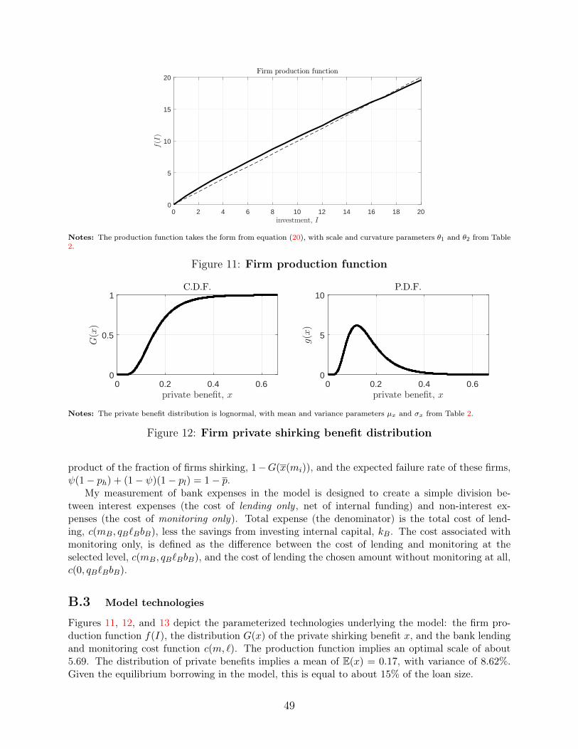
0 2 4 6 8 10 12 14 16 18 20investment, I

0

5

10

15

20

f(I)

Firm production function

Notes: The production function takes the form from equation (20), with scale and curvature parameters θ1 and θ2 from Table2.

Figure 11: Firm production function

0 0.2 0.4 0.6private benefit, x

0

0.5

1

G(x)

C.D.F.

0 0.2 0.4 0.6private benefit, x

0

5

10g(x)

P.D.F.

Notes: The private benefit distribution is lognormal, with mean and variance parameters µx and σx from Table 2.

Figure 12: Firm private shirking benefit distribution

product of the fraction of firms shirking, 1−G(x(mi)), and the expected failure rate of these firms,ψ(1− ph) + (1− ψ)(1− pl) = 1− p.

My measurement of bank expenses in the model is designed to create a simple division be-tween interest expenses (the cost of lending only , net of internal funding) and non-interest ex-penses (the cost of monitoring only). Total expense (the denominator) is the total cost of lend-ing, c(mB, qB`BbB), less the savings from investing internal capital, kB. The cost associated withmonitoring only, is defined as the difference between the cost of lending and monitoring at theselected level, c(mB, qB`BbB), and the cost of lending the chosen amount without monitoring at all,c(0, qB`BbB).

B.3 Model technologies

Figures 11, 12, and 13 depict the parameterized technologies underlying the model: the firm pro-duction function f(I), the distribution G(x) of the private shirking benefit x, and the bank lendingand monitoring cost function c(m, `). The production function implies an optimal scale of about5.69. The distribution of private benefits implies a mean of E(x) = 0.17, with variance of 8.62%.Given the equilibrium borrowing in the model, this is equal to about 15% of the loan size.

49

0 0.5 1 1.5 2loans, ℓ

0

1

2

3

c(m,ℓ)

Cost over lending

low m

mid m

high m

0 0.05 0.1 0.15 0.2monitoring, m

0

1

2

3

c(m,ℓ)

Cost over monitoring

low ℓ

mid ℓ

high ℓ

Notes: The cost function takes the form from equation (21), with loan and monitoring curvature parameters ρ1 and ρ2 fromTable 2.

Figure 13: Bank lending cost function

B.4 Computational algorithm

The computational algorithm employed to solve this model uses a grid search to find the bank andhousehold optimal policies nested within price updating based on excess demand functions in eachof three markets: bank loans, direct loans, and deposits. In this section, I lay out the key stepsof the algorithm in detail. Note that the estimation of the model involves embedding the stepsoutlined below within a standard SMM routine.

1. Fix the set of parameters in Table 2. Create grids for bank loans (`B), bank monitoring (mB),and household direct lending.

2. Compute the value of firms’ outside option, VO(kF ), according to (7).

3. Make an initial guess of the price vector, q0.

4. Taking these prices as given,

(a) use the loan size optimality condition (8) to compute the size of the loan demanded byfirms, b∗i , for i ∈ {B,H}.

(b) Solve the bank problem, taking b∗B as given:

i. For each pair of points on the grids for `B and mB,A. Use the bank budget constraint in (11) and current prices to compute the

amount of deposits the bank must take in to implement this policy, dB(`B,mB).38

B. Compute the total value associated with each choice using the objective func-tion in (11).

ii. Find the maximal value and the associated optimal policies, `∗B, m∗B, and d∗B =

dB(`∗B,m∗B).

(c) Solve the household problem, taking b∗H as given:

i. For each possible choice of `H ,

38In principle, the bank may want to take in no deposits and even lend less than its own internalcapital, kB. I allow for this in the algorithm by allowing the bank to invest in the storage technologyif lending is sufficiently unfavorable. Generically, this case does not arise.

50

A. Use the household budget constraint in (15) and current prices to compute theamount of deposits the household will supply at this policy, dH(`H).39

B. Compute the total value associated with each choice using the objective func-tion in (15).

ii. Find the maximal value and the associated optimal policies, `∗H and d∗H = dH(`∗H).

(d) Compute firm values from each type of lender, Vi(kF ), according to (7), taking mB asgiven for VB. Then, use (10) to compute the shares choosing each lender, Li(k).

5. Compute the excess demand function associated with the current prices, Z(q0) from (38).

6. If the convergence metric sup{|zB(q0)|, |zH(q0)|, |z(q0)|} is within the tolerance defined at theoutset, an equilibrium has been found. Go to step 9. Otherwise, proceed to steps 7 and 8.

7. Update prices according to:

q1 =

q1B

q1H

q1

=

(1− ν1)q0B + ν1(q0

B − ν2zB(q0))(1− ν1)q0

H + ν1(q0H − ν2zH(q0))

(1− ν1)q0 + ν1(q0 − ν2z(q0))

,where ν1 and ν2 are parameters which govern the speed and smoothness of convergence.Both parameters decline deterministically from iteration to iteration, so that prices adjustmore in early iterations and less in later iterations as the algorithm gets closer and closer toconvergence.

8. Set q0 = q1 and go back to step 4.

9. Use the equilibrium prices and quantities to compute desired model moments.

39If q = 1, the household is indifferent between deposits and the storage technology. In thiscase, the algorithm reflects this indifference via an updated market clearing, requiring only thatdH + aH ≥ dB. If q < 1, storage is strictly dominated.

51