saba shanfi - doras
TRANSCRIPT

1
C o - M o v e m e n t s a m o n g F i n a n c i a l S t o c k s
a n d
C o v a r i a n c e M a t r i x A n a l y s i s
Saba Shanfi
A dissertation submitted in partial fulfilment o f
the requirement for the degree o f
Master o f Science
Supervisor Dr Martin Crane
School o f Computing
Dublin City University
August 2003
i

Declaration
I hereby certify th a t th is m ateria l, w h ich 1 no w subm it fo r assessm en t on
the p rog ram o f study lead ing to the aw ard o f M .S c. in C om puting is
en tire ly m y ow n w o rk and has no t been tak en from th e w o rk o f o thers
save and to the ex ten t th a t such w o rk has been c ited and acknow ledged
w ith in the tex t o f m y w ork .
Signed:

f
I wish to thank all people who have been supporting and helping me during
my study especially when problems occurred
First of all my husband, Atid Shamaie, who always encouraged and guided
me even when he was busy with his own woik I learnt a lot from his discussions
and he was really a gieat help to me
I would like to thank the Modelling and Scientific Computing group
especially Prof Heather Ruskin for hei unfailing guidance and patience and also
Mi Gary Keogh for his very useful ideas and solutions to the problems
I sinceiely thank my supervisor Di Martin Crane for all his support before
and after I started with him as a postgiad student He gave me the opportunity to
study here and to attend to a very prestigious workshop in the University of
Oxford
Also, I wish to thank Cathal Guinn for kindly coriecting my chapters of
thesis and very friendly comments during its write-up, and Yaw Bimpeh for his
nice explanations Other friends who I would like to thank for their friendly
support are Paul Biown, Hyowon Lee, Thomas Sodnng, Null McMahon,
Michelle Toohei, Karl Podesta, Steven Harford, Qamir Hussain, Jiamin Ye and
Fajer Al-sayer
Acknowledgements

Abstract
The major theories of finance leading into the main body of this research are
discussed and our experiments on studying the risk and co-movements among
stocks are presented
This study leads to the application of Random Matrix Theory (RMT) The idea
of this theory refers to the importance of the empirically measured correlation (or
covariance) matrix, C, in finance and particularly in the theory of optimal
portfolios However, this matrix has recently come into question, as a large part
of it does not contain useful information but rather noise Therefore, recent work
has indicated that the theory of optimal portfolios, which depends on C, is not
adequate We use RMT in order to measure the noise component of C, and then
we examine the methods of differentiating noise from information We go on to
develop a novel technique of stability analysis for the eigenvectors of C after
noise removal
Further, changes in the portfolio associated with the riskiest position, (as given
by the largest eigenvalue and associated eigenvector), are investigated using the
results of the previous chapters From the results, we observe periods of co
movements of stocks, which change regularly because of some key events m the
market These periods are characterised by a linear relationship between price
and eigenvalue change However, the residuals in this model are strongly
dependent on granularity (1 e sampling rate) with fit breaking down at rates
smaller than five days Possible reasons for this breakdown are presented m
detail

CONTENTS
CHAPTERl
INTRODUCTION
1 1 Stock M arkets a r o u n d the w orld
1 2 Stock M arket In d ic a to r s
1 3 D erivatives
1 4 M ar k et d eclines
1 5 Scope of the thesis
CHAPTER 2
LITERATURE REVIEW
2 1 A r e v ie w o f M a r k o w itz p or i f o l i o t h e o r y
2 2 A r e v ie w o f C a p it a l M a r k e t T h e o r ie s a n d p r e d ic t in g m o d e ls
2 3 H is i o r i c a l c o v a r ia n c e m a i r ix , A p ro b lem2 31 Physical history
9
10
11
1213
CHAPTER 3
RANDOM MATRIX THEORY
3 1 R a n d o m M a t r ix p r e d ic t io n
3 2 E m pirically- m e a su r fd co rrflatio n m atrix
3 3 E ig e n v a lu e dis tribution of the co rrflatio n m atrix
3 4 S im ula i ion
3 41 Experimental analysis
3 5 A pplication to em pirical d a i a
3 6 N um erica l results
3 61 Eigenvector analysis
3 7 R M T p red ic t io n a n d p o r t i o l i o t h e o r y
3 8 Co nclusio n
17
17
18
19
20
2126
29
2931
32
33
C H A P T E R 4
M A T R IX S T A B IL IT Y
4 1 N o ise r e m o v a l fr o m c o r r e l a t i o n m a tr ix 411 Experimental analysis
4 2 O p tim a l p o r t f o l i o A s i a b i l i t y a p p r o a c h 4 21 Stability of the correlation matrix4 2 2 Stability of the cleaned correlation matrix
34
34
3538
424446

4 4 CONCI LSION
4 3 A \LW APPROACH lO MATRIX III TERING
52
47
CHAPTER 5 53
EPOCHS 53
5 1 V o i A m m 54511 Risk 55
5 2 M l i h o d o i o g y 56
5 3 E x p e r im e n t a i r i s l i t s 585 31 Epochs Definition 585 3 2 Epochs Discussion 60
D a t e 635 33 Epochs Models 635 3 4 Sampling rate analysis 65
5 4 POSSIBLL RLASO\S FOR MODEI FA III R r 6 6
5 5 C O \C I LSION 6 8
CHAPTER 6 69
CONCLUSIONS AND FUTURE WORK 69
• A PRAC1ICAI APPLICATION FOR I HI RLSl I T 01 R M T 71
• FbTLRI WORK 71
G l o s s a r y 7 3
R e f e r e n c e s 75
A p p e n d ix A 82
A p p e n d ix B 83C o d s 83
A p p e n d ix C 98T m P U B L IS in D PA PLR 9 8
A p p en d ix D 105T H h PRESI N TED PO STI R 105
A p p e n d ix E CDCD CD
D a t a CDM A T l AB C O D S CD

Chapter 1I n t r o d u c t i o n
A financial market is a market where financial assets are traded Although the
existence of a financial market is not a necessary condition for the creation and
exchange of an asset, in most economies, assets are created and consequently traded
in some type of financial market
The role of financial market is to indicate how the funds should be allocated among
assets as well as providing an environment, which forces or motivates an investor to
sell an asset [Fabozzi et a l, 1998] Because of these properties, it is said that a
financial market offers liquidity [Fabozzi et al, 1998], which is the ability of an asset
to be converted into cash quickly [Investor, 2003]
1

1 1 Stock Markets around the world
In terms of market value, the stock markets of the United States and Japan are the
largest in the world The third largest market, but far behind the United States and
Japan, is the UK market
Trading of common stock occurs in a number of trading locations such as “national
stock exchanges” or “over-the-counter” (OTC) markets [Teweles et a l, 1998] Stock
exchanges are made up of members who use the facilities to exchange certain
common stocks To be listed, a company must apply and satisfy requirements
established by the exchange [Fabozzi et a l, 1998] To have the right to trade stocks
on the floor of the exchanges, firms or individuals must buy a seat on the exchange,
l e they must become a member of the exchange A member firm may trade for its
own account or on behalf of a customer In the latter case it is acting as broker
The top national stock exchange in the United States is the New York Stock
Exchange (NYSE), popularly referred to as the Big Board It is the largest exchange
with over 3,000 companies’ shares listed
Unlisted stocks are also traded electronically in an over-the-counter market There
are about 5,000 common stocks included in the NASDAQ, the electronic quotation
system with a total market value of over $2 trillion (reported in NASDAQ web site
2003 [NASDAQ, 2003])
1 2 Stock Market Indicators
A stock market indicator (or index) is a statistical construct that measures price
changes and/ or returns in stock market The purpose of the index calculation is
usually to provide a single number whose behaviour is representative of the
movement of prices of all listed stocks and indicative of behaviour of the market as a
whole
The most commonly quoted stock market indicator is the Dow Jones Industrial
Average (DJIA) Other stock market indicators cited in the financial press are the
Standard & Poor’s 500 Composite (S&P 500), the New York Stock Exchange
Composite Index (NYSE Composite), the American Stock Exchange Market Value
Index (AMEX), the NASDAQ Composite Index, and FTSE 100
2

In general, market indices represent only stocks listed on one exchange Examples
are DJIA and the NYSE Composite, which represent only stocks listed on the Big
Board By contrast, the NASDAQ includes only stocks traded over the counter But
the most popular index is the S&P 500 as it contains both NYSE - listed and OTC -
traded shares The DJIA uses only 30 of the NYSE-traded shares, while the NYSE
Composite includes every one of the listed shares [Teweles et a l, 1998] The
NASDAQ also includes all shares in its universe, while the S&P 500 has a sample
that contains only 500 of the more than 8000 shares [Teweles et a l, 1998] FTSE 100
includes 100 most highly capitalised blue chip companies, representing
approximately 80% of the UK market [FTSE, 2003]
1 3 Derivatives
Derivative (or derivative security) is a financial instrument whose value depends on
the values of another asset Derivative markets have an important role in ‘risk
management’ and 'price discovery’ [Hull, 2000, Chance, 1995] as they enable
investors with a lower level of risk preference to transfer the risk to the investors
with higher level of risk preference “Future” and “forward” contracts are agreements
whereby two parties agree to transact some financial assets at a predetermined price
at a specified future date One party agrees to buy the financial asset, the other agrees
to sell the financial asset Both are obligated to perform, and neither party charges a
fee unless they do not want to perform the contract
Option contract, the other substantial derivative, gives the owner of the contract the
right, but not obligation, to buy (or sell) a financial asset at a specified price from (or
to) another party The buyer of the contract must pay the seller a fee, which is called
the option price
1 4 Market declines
When a crash occurs on the market all the people around the world suffer directly or
indirectly and millions of Dollars are lost Investors lose their money overnight and
the entire economy is affected The largest single day decline in the history of most
of the world’s stock markets, occurred on Monday, October 18, 1987 On that day,
3

popularly referred to as Black Monday the DJIA lost 22 6% and S&P500, 20 5% of
their total values and other market indexes declined to a similar extent [Roll, 1988]
On Black Monday Wall Street lost 15,000 jobs in the financial industry [Facts, 2002]
and all outstanding US stocks declined to approximately one trillion dollars [Sopns,
2002] Also a record loss of £50 6 billion on the London Stock Exchange was
proceeded by the fall of Wall Street [Guardian, 2003]
Market situation at present is represented by a prolonged decline plus a high
volatility that analysts describe it as a period of low returns and high risk, which will
be continued far into the future [Business, 2003c] This critical decline is exposed in
the S&P500, which has lost 45% of its value from March 2000 to March 2003
together with considerable volatility, six declines and five rises over the three years
The rallies and declines show how fast the market is changing investors’ portfolio
values In contrast to the last decade, the average length of the rallies over the last
year was only 74 days before the market slumped 10% whereas for 7 years when the
market climbed from October 1990 to October 1997 there was no decline of this size
[Business, 2003a] Stocks are swinging up and down now, more often than any time
since 1938 [Business, 2003b] As recently as 1995, the S&P 500 traded all year
without once changing 2% in a day but in 2002, it swung that much or more on 52
days [Business, 2003b]
Clearly, war with Iraq, and threat of terrorism made for a nervous market during last
year Millions of buy-and-hold investors, who have been a major stabilising force in
the stock market, are bailing out [Business, 2003b]
Figure 1 1 represents evolution of the four major indexes around the world over the
last decade The volatility and decline of the market are clearly seen over recent
years, in comparison with previously The other general message, here, is that the
market is reverting to pre-mid 90’s levels
4

Figure 1 1 A decade market evolution of (a) DJIA, (b) NASDAQ Composite, (c) S&P500 and (d)FTSE 100
Also it is useful to look at the currency situation, where Euro has been hardly
appreciating versus US Dollar since last year Figure 1 2 shows Euro-US-Dollar
movement over the last three years The US Dollar is in a worsening condition
against the Euro such that as of time of writing1 it has hit a 4-year low against Euro
1 To the date of 10 March 2003
5

2000 2001 2002
Figure 1 2 US Dollar dropping versus Euro over last three years The lowest is the last day shown l e10 March 2003
However, market volatility is the investors’ intensive concern as it determines
whether profit or loss on their portfolios is going to take place Today, a financial
analysts’ job is to determine a reasonable estimation of what the future market
behaviour will be and how the customers’ portfolio value is going to change He or
she will design the best portfolio for their clients to optimise the nsk-return
relationship on the combined assets in the portfolio That is the importance of
analysing and predicting the market future, which has reached a significant place in
the field of finance Estimating the future value of a portfolio and the probability of
how likely it is to be realised requires some features and instruments that have
introduced a new field in finance, known as portfolio management or investment
strategy [Fuller et a l, 1987] The first element of investment strategy is how to
combine assets to gain the most return with respect to the level of risk associated
with each investment Indeed, different investors have different levels of risk
preferences [Fuller et a l, 1987] Some people prefer to deal with a low-risk
investment even though it has a lower level of return Others prefer the chance of
gaining high return from their investment despite increased risk An optimisation
process, however, can imply sets of assets that result in either most return for a fixed
level of risk (dependent on the investor’s risk preference) or the lowest amount of
risk for a fixed level of return [Elton et a l, 1981 ] In any such process, the way that
stocks move together is an essential element to be studied The problem of how
stocks mter-relate is determined by the correlation coefficient, which measures co
movements between different stocks [Elton et a l, 1981] For a set of assets combined
6

in a portfolio, the correlation coefficients between each pair of stocks can be
displayed in a correlation matrix
1 5 Scope o f the thesis
In Chapter 2, we talk about theories of portfolio management citing key literature on
the area More details about the important role of the correlation matrix of stocks in
the portfolio management are explained, and the difficulties in calculating this matrix
are demonstrated
In Chapter 3, of this thesis, we discuss error problems inherent in the structure of
such correlation matrices This error problem occurs for several reasons, such as the
finite number of records in the stock’s prices To distinguish the error in the
correlation matrix, C, a technique, known to random matrix theory (RMT), is applied
[Laloux et a l, 1999] This allows us to differentiate the error from true information
In this chapter, also, we demonstrate a simulation approach to study the result of
RMT, when scattering (or noise) in stock’s prices is not in the same
In Chapter 4, methods of removing errors m C are investigated However, the
stability of the matrix is the important matter, which should be preserved in all cases
Accordingly, we apply a statistical model introduced by Krzanowski (1984) to
examine the stability of C after removing errors from that Our results indicate that
the stability of the matrix notably reduces and therefore, the analysis on that cannot
be, simply, reliable The method deals with the stability of eigenvalues and
eigenvectors of C, in which for a small change in an eigenvalue, it measures the
changes of eigenvectors Concerning this method, we extract a new method of
removing errors in the way that stability of the matrix is mostly kept
In the last chapter we take the most reliable part of the correlation matrix, which is
the maximum eigenvalue, to study the movement of the market The largest
eigenvalue of the correlation matrix is always an effective measure of risk and the
corresponding eigenvector represents the most-risky combination of stocks
Therefore we focus on the daily changes of the maximum eigenvalue to investigate
7

the risk on the set of stocks This study is based on a theorem in linear algebra called
the Spectral Theorem, and suggests a method to measure the day-to-day changes of
the correlation matrices Our results demonstrate a linear relationship between the
changes m eigenvalues’ ratio and the changes in the prices of the stocks We model
this relationship and discuss possible causes and breakdowns of the model
Finally, an overall conclusion plus some explanation about the future work is
presented
8

1
Chapter 2
Literature Review
In order to gain the most return from the set of assets of which it consist a portfolio
we need to estimate the risk and return of the portfolio In this chapter, we review the
literature in “portfolio theory” [Elton et a l , 1981] that leads to the problem of risk
prediction Different parts of this process include the study of correlations among
stocks and the risks associated with individual assets In this study, also, we review
other risk measurements used in “Capital Asset Pricing Model” [Fuller et a l , 1987],
which is one of the most important models in finance This chapter leads up to the
point of my project and a history about that We start by considering “Markowitz
portfolio theory” [Markowitz, 1991]
9

2 1 A re v ie w o f M a r k o w itz p o r t fo l io th e o ry
The modern portfolio theory developed by Markowitz m the early 50s [Markowitz,
1952] shows how to measure the risk associated with various securities and how to
combine these securities in a portfolio to get the maximum return for a level of risk
that investors are willing to accept
The cornerstone of the theory of Markowitz is the concept of “diversification”
Diversification is a portfolio strategy to reduce the risk by combining a variety of
investments It implies that as the number of various stocks gets higher, the overall
risk of the combined portfolio gets lower Strongin et al (2000) indicate that the risk
of the portfolio is always a function of where N is the number of distinct
assets
One of the results of the theory of Markowitz is the clarification of the definition of
risk Before hts theory of modern portfolio, there were other definitions for risk like
the one suggested by Graham et al (1962) Graham et al defined risk as a “margin of
safety”, based on the idea that the analyst should independently estimate the value
for the security in respect of its earning power and financial characteristics and
despite the market price
Also another definition by Sharpe (1981) considers the below-the-mean variability,
since, for most investors, risk is related to the chance that future portfolio values will
be “less” than expected However, empirical studies have shown [Blume, 1970] that
it makes little difference whether one measures variability of returns on one side or
both sides of the expected return Since working with the below-the-mean variability
is not easy, total variability of returns has been used widely as a proxy for risk and
the most commonly used measures have been the variance and standard deviation of
return [Fuller et a l , 1987] In general standard deviation is preferable because the
standard deviation of a portfolio’s return can be determined from the standard
deviations of the returns of its component securities [Sharpe, 1981] No other
variability measures are as simple to use as standard deviation Therefore the risk or
variability of a portfolio consist of N assets is measured as
10

N N^ X , X t a ik ’ (2 1)
1=1 i=l k =1 k*i
(where o] is the variance of component security i and X t are the fractions of the
investor’s funds invested in the security i and o lk is the covariance between security
1 Tl and security k expressed as o ik - — ̂ (rtJ - jut )(rkj - juk) , m which T is the number
T J=i
of records for each asset and jut is the average of assets / records and r is the return
on the ilh asset)
2 2 A review o f Capital M arket T heories and p red icting m odels
After the theory of Markowitz developed, there was a need to implement it in the real
world Sharpe in 1961 in his PhD dissertation created the basis for a practical model
called the “single-index model” or “one-factor model” The major assumption of this
simplified model is that all the co-movements of stocks can be explained by a single
factor One version of the model called the “market model”, uses a market index
such as the S&P 500 as the factor affecting stock movements [Elton et a l , 1981]
According to the market model it is assumed that when the market goes up most
stocks tend to increase m price, and when the market goes down, most stocks tend to
decrease in price
As well as the single-index model, King (1966) presented evidences on the existence
of other factors beyond the market factor He measured effects of common
movements among stocks beyond market effects and found an additional covariation
of stocks associated with industry This model is one of the family of “multi-index
model” [Elton et a l , 1981] Although multi-index models attempt to capture some of
the non-market factors and, hence to incorporate additional information, they fail to
provide a better description of the stocks behaviour That is because the cost of
introducing additional indices increases the chance to pick up random noise rather
than real information Elton et al (1973), and (1978) study “averaging techniques” to
predict the co-movements among stocks Such techniques smooth the entries in the
11

historical correlation matrix to reduce random noise and so provide a better forecast
However, the disadvantage of averaging models is that real information may be lost
All the models described above are statistical and are used to explain the covariance1
between asset returns There is also an economic model of equilibrium returns which
includes Capital Asset Pricing Model (or CAPM), one of the most famous of all
financial models [Fuller, 1987] This model has been developed by Sharpe (1964),
Lintner (1965), and Mossin (1966) in 1960s and it is based on the idea that investors
demand additional expected return (called risk premium) if asked to accept additional
risk The expected return of a stock equals the rate on a risk-free asset plus a risk
premium According to CAPM, risk is defined in terms of volatility, and it is
measured by the investment’s f i 2 coefficient, which is the ratio of covariance
between stock’s return and market’s return to the variance (or volatility) of the
market This type of risk was identified by Sharpe (1964) to be “systematic risk”, and
also known as “market risk” Since systematic risk is only associated with the
market, it cannot be diversified away Beside the systematic risk, there is
“unsystematic risk”, which is the risk specific to a company’s fortunes and can be
reduced by increasing the number of various assets
An alternative asset-pricing model to the CAPM was created by Ross (1976) and it is
called the Arbitrage Pricing Model (or APT) Unlike CAPM, APT may specify
return on an asset as a (linear) function of more than one single factor The strength
of this model lies in the fact that it is based on the no-arbitrage condition, which
means that two identical or similar items cannot be sold at different prices on
different markets
2 3 H istorical covariance m atrix , A problem
Implicitly, in all the theories and models we have mentioned so far, the calculation of
the covariance matrix is required as a practical stage For example in the first step of
calculating the historical portfolio risk one needs to construct the covariance matrix
1 A measure of the co-movements of two assets
2 = -̂ V2tm , m which Covtm is the covariance between ith stock and market and <j2m is thecrM
variance o f the market
12

on a past period Also for estimating ¡3 in the models mentioned, the need to
calculate the historical covariances between a huge number of stocks can be seen
Studying the correlation3 (or covariance) matrix, C, is also of great interest in data
analysis in order to extract information from experimental signals or observations
e g in pattern recognition [Theodondis et a l , 1999], weather forecasting [Jolliffe et
a l , 2003], and economic data analyses [Laloux et a l , 1999] Moreover, many
statistical tools such as principal component analysis and factor analysis [Kim et a l ,
1979] try to obtain the meaningful part of the signals in a correlation matrix in order
to reduce the dimensionality of the data set
However, use of this matrix, C, which has been widespread over decades, came into
question as two different research groups realised that a large part of it does not
include useful information but rather significant errors [Laloux et a l , 1999, Plerou et
a l , 1999] Laloux et al (1999) and Plerou et al (1999) simultaneously worked on the
application of some physical theories, (discussed below), in the field of finance and
concluded that C does not include pure information In particular, the difficulties
associated with determining the true correlations between financial assets arise
primarily due to
• Non-stationary4 nature of the correlations between stocks
• A finite number of observations of asset price movements
The issue then becomes how to identify the true correlated assets when there is error
in the measured correlations
2 3 1 Physical history
In their book, Mantegna and Stanley (2000) stated that, since 1990, a growing
number of physicists have attempted to analyse and model financial markets The
interest of these people in financial systems was initially stimulated by work such as
that of Majorana (1942) on the essential analogy between statistical laws in physics
and in the social sciences In 1999 similarities between correlations in financial and
physical time series were noted by two different groups of physicists [Bouchaud et
3 which differ from covariance matrices in having the variance normalised out4 It means the correlation between any two pairs of stocks changes with time
13

a l , 2000, Plerou et a l , 1999] Plerou et al (2000a) explained that financial markets
are examples of complex systems in which a huge amount of data exist The
correlations between the price changes of stocks can be compared to those of
movements of molecules in a box containing many gas molecules, in which there are
some random pair-wise bonds between some of the gas molecules Alternatively, in a
more complicated system, not just random pair-wise bonds are involved, but rather
bonds connecting clusters of molecules, which evolve over time Thus, new
molecules are connected to the existent clusters and others, which are part of one
cluster, connect to different clusters
In all these cases one can calculate the empirical measured correlation matrices but in
Finance, unlike for most physical systems [Plerou et a l , 2000b], there is no
algorithm to calculate the “interaction strength” between two companies and there
are difficulties in quantifying stock correlations
A further difficulty is that of strictly limited number of observations, which causes
random errors in correlation matrices (as mentioned above)
In nuclear physics, the problem of understanding the properties of matrices with
random entries has a rich history beginning with the work of Wigner (1951a, 1951b,
and 1956) and subsequently Dyson (1962, 1963) and Mehta (1963, 1991) In the
fifties, physicists faced the problem of understanding (and measuring) the energy
levels of complex nuclei5, which existing sub-atomic particle models failed to
explain Large amounts of data on the energy levels were becoming available but
were too complex to be explained by model calculations because the exact nature of
the interactions was unknown To solve this problem, Wigner (1951a, 1951b) made
the assumption that the interactions between the constituents comprising the nucleus
are so complex that they can be modelled as random Then, he assumed that the
Hamiltonian6 describing a heavy nucleus7 could be described by a matrix H with
independent random elements Based on this assumption, Wigner (1956) derived
properties for the statistics of eigenvalues of the random matrix H whose elements
5 The nucleus, like the atom, has discrete energy levels [Ernest Orlando Lawrence Berkeley
National Laboratory, http //wwvv lbl gov/abc/wallchart/teachersguide/pdf/Ch06-
EncrgyLevcls%20doc pdf ]
d Hamiltonian is a scries of operators associated with the system energy
7 Heavy nuclei are composed of many interacting constituents
14

are mutually independent random variables Eventually he found these properties in
remarkable agreement with experimental data [Wigner, 1956]
A long time of about three decades after this result in nuclear physics, Laloux et al
(1999) applied Random Matrix Theory (RMT) to finance and showed that C can be
partitioned into noisy and non-noisy components From a more formal mathematical
point of view, this phenomenon was studied also by a group at the University of
Boston by Plerou et al (1999) In their own independent research they used the
method of RMT to study the correlations of stock price changes
Based on this earlier work on RMT in Finance, Bouchaud and Potters (2000) argued
that Markowitz’s theory of optimal portfolio is not adequate on its own Therefore, in
[Laloux et a l , 2000] the authors introduced a technique to remove noise from the
matrix by cleaning the noisy band and they suggest that the risk of the optimised
portfolio obtained using a cleaned correlation matrix is more reliable They,
therefore, claim that the cleaned correlation matrix is more stable Plerou et al
(2000b, 2001b) and Mounfield et al (2001) discuss the stability of C by examining
the overlap (i e measured by scalar product) of its eigenvectors over two consecutive
sub-periods For those showing higher overlap (values near unit) over two sub
periods, the stability is assumed to be higher and for those showing lower overlap
values, stability is lower The evidence suggests that the part of C known as noisy (in
RMT), tends to show lower level of stability (in overlap)
In research on techniques of Principal Component Analysis [Jolliffe, 1986] the
stability of the eigenvectors is also studied Green (1977) and Bibby (1980) discuss
the rounding effect of Principal Components (PCs) on the variance (eigenvalues) of
the matrix They show that rounding PCs to a few decimal places does not make a
great change though the Principal Components are no longer exactly orthogonal
Krzanowski (1984), however, considers the opposite problem Instead of looking at
the effect of small changes in the eigenvectors on the eigenvalues, he examines the
effect of small changes of the eigenvalues on the eigenvectors He then argues that
this gives important information on the stability of Principal Components [Jolliffe,
1986] It is thus possible, using the Krzanowski technique, to examine the stability of
C before removing noise and afterwards This demonstrates how noise-removing
methods can effect the stability of the modified correlation matrix and how a
cleaning method, in general, can preserve the stability behaviour of the correlation
15

matrix This is discussed in detail in the following chapters with experimental results
used to demonstrate these points for our data
The focus of this review has been
(a) topics in our project and literature on the area,
(b) noise m the correlation matrix,
(c) stability behaviour of the correlation matrix
Practical implementations are demonstrated in the following chapters Further, we
bring together a number of these features in the study of co-operative behaviour in
market, [Crane et a l , 2002, Keogh et a l , 2003] in chapter 5
16

Chapter 3R a n d o m M a tr ix T h e o ry
We study the basis for applying Random Matrix Theory (RMT) on an empirically-
measured correlation matrix, C, of financial data type and demonstrate that this
matrix contains a large amount of noise
Firstly, we simulate a set of data and add different volumes of random noise to see
the results of the theory on each data set
Secondly, we apply RMT on empirical data and estimate the percentage of noise in C
using eigenvalue and eigenvector analysis The experimental results for each of them
are presented
17

3 1 R a n d o m M a t r ix p re d ic t io n
Wigner (1956) and Dyson et al (1963) describe Random Matrix predictions as an
average of all possible interactions in a nucleus Additionally, they explain that
deviations from the universal predictions of “Random Matrix Theory” identify non-
random properties that are specific to the considered system
Agreement between the distribution of the eigenvalues of a matrix M, with those
from a matrix made up of random entries implies that M has entries that contain a
considerable degree of randomness, as has been shown in the literature [Plerou et a l ,
2000b, Laloux et a l , 1999] This matrix made up of random entries with unit
variance and zero mean is called a random matrix [Mehta, 1991] In the case of a
correlation matrix, agreement between eigenvalues’ distribution of C and those from
a random matrix, represents randomness (or noise) and therefore deviations from
RMT represent genuine correlation [Plerou et a l , 2000a] This is exactly our
problem, to identify the true information ( 1 e correlated assets) among noise (or
randomness) in the financial correlation matrix The method is to compare the
distribution of eigenvalues of correlation matrix against the “null hypothesis” of a
random matrix Since the correlation matrix is symmetric the random matrix, which
it is compared to, should also be symmetric [Plerou et a l , 2001b] Any agreements
between them should pinpoint noise and any deviations should reflect genuine
correlated assets In other words, the part of the correlation matrix that has the same
behaviour as the random matrix is considered to be the noisy part while that which
contains information, is considered to be non-noisy
3 2 E m pirically-m easured correlation m atrix
Normally, the price changes (or return) of stocks are employed to quantify the
empirical correlation matrix [Plerou et a l , 2001a] Therefore, we need to calculate
the price changes of assets /= /, , N over a time scale At For a price S t(t) of the
ith asset at time /, one can define its price change/ return G, (/) as
Gf(0 = ln S, (/ + Af)“ ln St (t) (3 1)
18

It should be noticed that the terms “return” and “price changes” are sometimes used
interchangeably (as in [Plerou et a l , 2001a] for instance) but strictly speaking, they
are different
Also, it needs to be mentioned that different stocks have varying levels of volatilities
In the literature review chapter (chapter 2), we explained that volatility or risk
associated with the stock’s price changes can be measured by its variance (or
alternatively standard deviation) With respect to various standard deviations for
different time series, one usually defines a normalised return to standardise the
different stock volatilities Therefore, we normalise G, with respect to variance cr
as follows
where <rt is the standard deviation of G, for assets i=J, ,N and G, is the time
average of Gt over the period studied
There is a standard definition [Plerou et a l , (2000b), (2001a)] for the correlation
matrix C, with elements Cy,
Here the bar denotes a time average over the period studied In matrix notation, the
correlation matrix can be expressed as
where G is an N x f matrix with elements {g,(/w)> l ~ \ , N i m = 0, ,7 - 1 ) , T is
the number of records and G T denotes the transpose of G
(3 2)
C 9 = g , ( t ) g J ( 0 (3 3)
C = —GGr , 7
(3 4)
19

3 3 E ig e n v a lu e d is t r ib u t io n o f the c o r re la t io n m a tr ix
As stated above, our aim is to extract real information about correlations from C So,
the properties of C are compared with those of a random correlation matrix as has
been done by Laloux et al (1999) and Plerou et al (1999) According to Equation
3 5 a “random” correlation matrix R is considered [Plerou et a l , 2001b] as,
R = j AAt (3 5)
where A is an N x T matrix containing N time series of 7 random elements with zero
mean and unit variance, which are mutually uncorrelated Statistical properties of
random matrices such as R have been known for many years in physical literature
[Dyson, 1971, Edelman, 1988, Sengupta et a l , 1999] Particularly, under the
Tcondition of 7 ->oo, N -»ao and providing that q ~ — > 1 is fixed, it was shown
[Sengupta et a l , 1999] that the distribution of eigenvalues A of the random
correlation matrix R is given by
2 n a l0
A2 < X <X.
elsewhere(3 6)
where a 2 is the variance of the elements of G, (in the case of a normalised matrix G,
it is therefore equal to unity), and Am:n and Amax are the minimum and maximum
eigenvalues of R respectively, given by
¿max = CT2(1+ —± 2 E ) (3 7)m in q y q
These are the theoretical maximum and minimum eigenvalues that determine the
bounds of the theoretical distribution of eigenvalues All the eigenvalues of the
20

random matrix are located between these two values. If eigenvalues of C are beyond
it is said that they deviate from the random (or theoretical) bound.
To see the results of RMT in practice we apply it first on generated data (a novel
approach) and second on a set of real data. With generating data and having the
advantage of controlling the volume of noise, we aim to examine the effect of
different volume of added noise on the result of RMT. While using real data is the
main purpose to approximate noise in a real historical correlation matrix.
3.4 S im ulation
In order to see the results of RMT on a correlation matrix made up of a simulated
data we generate a set of sinusoidal random time series. A set of 450 sinusoidal time
series with 1500 observations (i.e. the same size as our real data set) is generated
with random amplitude and random phase. Figure 3.1 shows some of these time
series.
1000Observations
Figure 3.1 Randomly generated sinusoidal time series
1500
21

Valu
e
0 8 1 1--------------------------0 500 1000 1500
Observation
(a)
Observation
(b)Figure 3 2 A sinusoidal tunc scries with added random noise (a) with noise standard deviation equal
to 0 02, (b) with noise standard deviation equal to 4
22

Next, we add some random noise normally distributed with zero mean and a
particular standard deviation to the time series We control the volume of noise
added to the generated data by changing its standard deviation Figure 3 2 shows one
of the time series with two different volumes of added noise In Figure 3 2(a) the
time series is quite clear, while, in Figure 3 2(b), it is mainly dominated by noise We
study the behaviour of the correlation matrix constructed from those noisy time
series by applying RMT in order to see the effect of different volumes of noise in
time series on noise in C
First by using Equation 3 3 the correlation matrix C is constructed Since the number
of observations is T=1500 and the number of time series is N=450 the inequality
q ~ -jj; > 1 is satisfied Therefore, we can apply the RMT to our generated data and
plot the distribution of the eigenvalues of C
0 0 5 1 15 2 25Eigenvalues
Figure 3 3 The theoretical distribution of the eigenvalues of the generated random matrix
23

Dist
rubu
tion
Dis
trub
utio
n
Eigenvalues
( a )
Eigenvalues
(b)Figure 3.4 (a) The empirical distribution (solid line) and the theoretical distribution (diamonds) of
eigenvalues, (b) a closer look at the beginning part of the graphs.
24
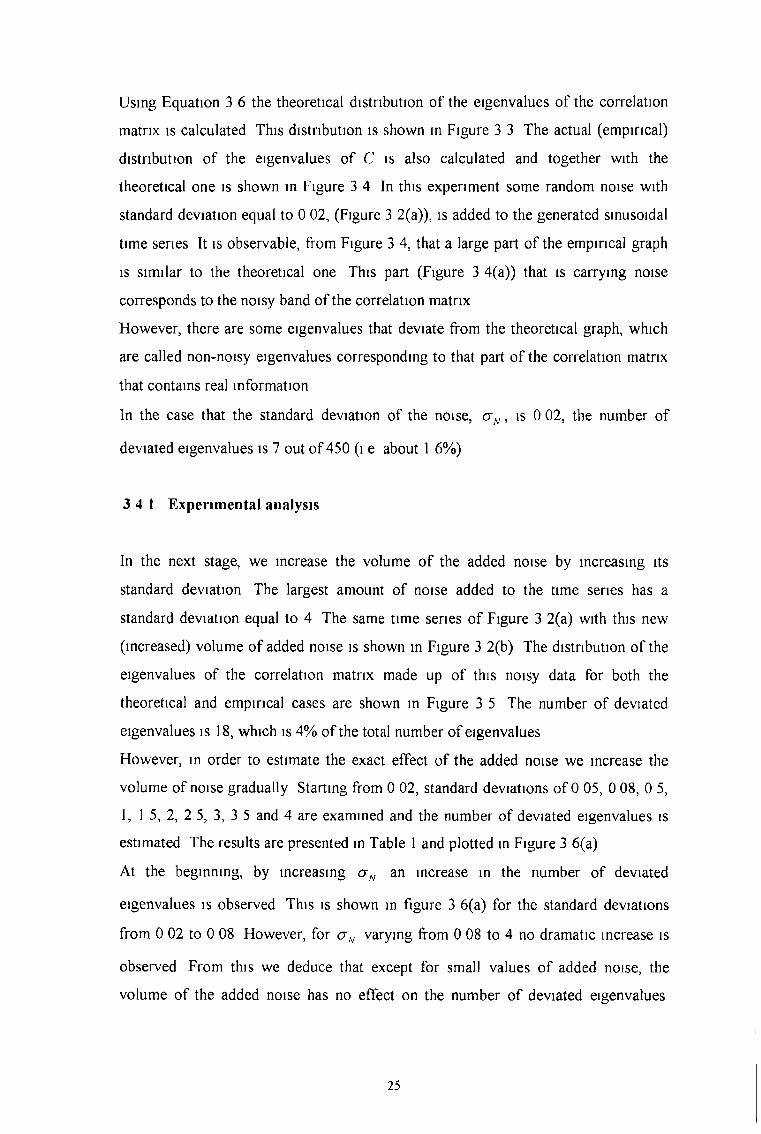
Using Equation 3 6 the theoretical distribution of the eigenvalues of the correlation
matrix is calculated This distribution is shown in Figure 3 3 The actual (empirical)
distribution of the eigenvalues of C is also calculated and together with the
theoretical one is shown in Figure 3 4 In this experiment some random noise with
standard deviation equal to 0 02, (Figure 3 2(a)), is added to the generated sinusoidal
time series It is observable, from Figure 3 4, that a large part of the empirical graph
is similar to the theoretical one This part (Figure 3 4(a)) that is carrying noise
corresponds to the noisy band of the correlation matrix
However, there are some eigenvalues that deviate from the theoretical graph, which
are called non-noisy eigenvalues corresponding to that part of the correlation matrix
that contains real information
In the case that the standard deviation of the noise, crN, is 0 02, the number of
deviated eigenvalues is 7 out of 450 ( 1 e about 1 6%)
3 4 1 Experimental analysis
In the next stage, we increase the volume of the added noise by increasing its
standard deviation The largest amount of noise added to the time series has a
standard deviation equal to 4 The same time series of Figure 3 2(a) with this new
(increased) volume of added noise is shown in Figure 3 2(b) The distribution of the
eigenvalues of the correlation matrix made up of this noisy data for both the
theoretical and empirical cases are shown in Figure 3 5 The number of deviated
eigenvalues is 18, which is 4% of the total number of eigenvalues
However, in order to estimate the exact effect of the added noise we increase the
volume of noise gradually Starting from 0 02, standard deviations of 0 05, 0 08, 0 5,
1, 1 5, 2, 2 5, 3, 3 5 and 4 are examined and the number of deviated eigenvalues is
estimated The results are presented in Table 1 and plotted in Figure 3 6(a)
At the beginning, by increasing a N an increase in the number of deviated
eigenvalues is observed This is shown in figure 3 6(a) for the standard deviations
from 0 02 to 0 08 However, for crv varying from 0 08 to 4 no dramatic increase is
observed From this we deduce that except for small values of added noise, the
volume of the added noise has no effect on the number of deviated eigenvalues
25

Consequently, we conclude that the number of non-noisy eigenvalues is independent
of added noise. On the other hand, in Figure 3.5 it is shown that the maximum
eigenvalue of C, say max(e), for the case when crN= 4, is closer to the A ^ ,
theoretical maximum value from Equation 3.6, than max(e) when <7̂ =0.02, Figure
3.4(a). This motivates us to investigate the effect of the volume of added noise on the
distance between A ^ and max(e). For the same experiments as Table 3.1 this
distance is examined and the result is plotted in Figure 3.6(b). Again it is seen that
after the first few points, which show the maximal differences, the rest of them fall
on an almost horizontal line. Again showing that ( A ^ - max(e)) is almost
independent of added noise.
We also computed the eigenvalues of an ideal C with absolutely no noise. Only two
of the largest eigenvalues are non-zero and the rest are all zeroes. Additionally, those
non-zero eigenvalues are much larger than A^ . This means that as C approaches the
ideal correlation matrix, more eigenvalues approach zero and the difference between
the smallest and largest eigenvales (that has a value of about 260) is significant. That
is the reason why we see less deviated eigenvalues for a very low volume of noise in
our experiments, i.e. g n =0.02.
Eigenvalues
Figure 3.5 The empirical distribution of eigenvalues (solid line) and the theoretical distribution (diamonds). Added noise with standard deviation equal to 4
26

diffe
rece
be
twee
n m
axim
um
eige
nval
ues
Num
ber
of de
viat
ed
eige
nval
ues
Noise standard deviation
Noise standard deviation
Figure 3.6 Relationship between the number of deviated eigenvalues from the noise band and thevolume of noise
27

Noise STDV 0 02 0 05 0 08 05 1 1 5 2 2 5 3 3 5 4# deviated
eigenvalues 7 15 17 17 18 18 18 17 18 17 18
Table 3 1 The volume of noise versus the number of deviated eigenvalues
The implications really are that the strong signal core is shown by this method and is
contained in a few relatively unaffected values
3 5 A pplication to em pirical data
The set of data we have for our experiments consists of 30-minute intra-day prices
from S&P500 over the period started from the beginning of April 1997 to the
beginning of April 1999 Since the number of observations (records) is important for
using RMT, the intra-day data can provide a large number of records on an even
small period of time This set of data with about N=450 companies, and over
1=1500 observations is appropriate for our purpose since according to the constraint
on using Equation 3 5, q - - ~ > 1 is satisfied
3 6 N um erical results
Firstly, we construct the empirically-measured correlation matrix C by using the
Equation 3 6 as in the previous section, and then compute the eigenvalues Xk where
k=l, , N is in ascending order
The distribution of the eigenvalues of the corresponding random correlation matrix is
also calculated using Equation 3 6 Figure 3 7 shows the results of our experiments
on the 30-minute data for 452 stocks and 1500 records The same as the results of
RMT on the simulated data we can observe two things from Figure 3 7
• The bulk of the eigenvalues of C conform to those of a random matrix with
graphs consistent with the latter This consistency means that there is a measure
of randomness in the bulk of the eigenvalues Therefore, as stated in [Laloux et
a l , 1999] we conclude that the corresponding part of eigenvalues is random and
we consider this part as the noisy band
28

Eigenvalues
(a)
Eigenvalues
(b)
Figure 3.7 (a) Eigenvalue distribution for C constructed from the 30-minute prices for 452 stocks of S&P 500 for 1500 records started from April 1997. The diamond curve shows the RMT result for
Pr(%) in Equation 3.6. Several eigenvalues outside the RMT upper hound can be seen, (b) awider view of the graph (a) including the highest eigenvalue
29
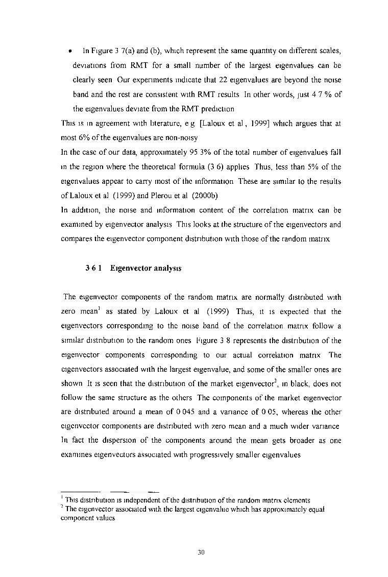
• In Figure 3 7(a) and (b), which represent the same quantity on different scales,
deviations from RMT for a small number of the largest eigenvalues can be
clearly seen Our experiments indicate that 22 eigenvalues are beyond the noise
band and the rest are consistent with RMT results In other words, just 4 7 % of
the eigenvalues deviate from the RMT prediction
This is in agreement with literature, e g [Laloux et a l , 1999] which argues that at
most 6% of the eigenvalues are non-noisy
In the case of our data, approximately 95 3% of the total number of eigenvalues fall
in the region where the theoretical formula (3 6) applies Thus, less than 5% of the
eigenvalues appear to carry most of the information These are similar to the results
of Laloux et al (1999) and Plerou et al (2000b)
In addition, the noise and information content of the correlation matrix can be
examined by eigenvector analysis This looks at the structure of the eigenvectors and
compares the eigenvector component distribution with those of the random matrix
3 6 1 Eigenvector analysis
The eigenvector components of the random matrix are normally distributed with
zero mean1 as stated by Laloux et al (1999) Thus, it is expected that the
eigenvectors corresponding to the noise band of the correlation matrix follow a
similar distribution to the random ones Figure 3 8 represents the distribution of the
eigenvector components corresponding to our actual correlation matrix The
eigenvectors associated with the largest eigenvalue, and some of the smaller ones are
shown It is seen that the distribution of the market eigenvector2, in black, does not
follow the same structure as the others The components of the market eigenvector
are distributed around a mean of 0 045 and a variance of 0 05, whereas the other
eigenvector components are distributed with zero mean and a much wider variance
In fact the dispersion of the components around the mean gets broader as one
examines eigenvectors associated with progressively smaller eigenvalues
1 This distribution is independent of the distribution of the random matrix elements2 The eigenvector associated with the largest eigenvalue which has approximately equal component values
30

Although the eigenvector analysis we have done is not as precise as the eigenvalue
analysis above, it does suggest that the market eigenvector behaves differently to the
eigenvectors of the random matrix and, therefore, represents the most reliable part of
the correlation matrix.
So far, it has been shown that the results from the theory of random matrices are of
great interest in understanding the statistical structure of the empirical correlation
matrices. The central result of this study is in recognising that there exists a large
amount of noise in the eigenvalues and corresponding eigenvectors of C.
30
25
20
c01 15IsQ
10
5
0-0.15 -0.1 -0.05 0 0.05 0.1 0.15 0.2 0.25 0.3
Eigenvector components
Figure 3.8Distribution of eigenvector components
3.7 R M T prediction and portfolio theory
We have noted specifically that the risk associated with a particular portfolio
consisting of N assets, which can be expressed (in some sense) as the total variance
cr2p , in which the risk is directly associated with the correlations between stocks. In
31

portfolio optimisation, <j2 should be minimised for a given value of the return of the
portfolio, Rp The result of the optimisation analysis indicates that the smallest
eigenvalue is associated with the “least risky portfolio” and the corresponding
eigenvector determines the weights (or fraction) of stocks in the portfolio (as stated
in [Chan et a l , 1999, Alexander, 2001] for instance) Therefore, the composition of
the “least risky portfolio” has a large weight on the eigenvectors of C corresponding
to the smallest eigenvalues
However, from the RMT results, we saw that the smallest eigenvalues of C and
corresponding eigenvectors are not trustworthy, as they contain a large amount of
noise Therefore, Markowitz’s portfolio theory, which depends on a purely historical
correlation matrix, comes into question as the smallest eigenvalues of C (determining
the smallest nsk-portfolio) are dominated by noise
This shows the importance of differentiating noise from information in C In the next
chapter we use the suggested noise removal method by Bouchaud et al (2000) and
discuss on it in detail
3 8 C onclusion
We have applied Random Matrix Theory to determine the noise in an empirically-
measured correlation matrix, C For a set of actual data from S&P500 we found that
approximately 95% of eigenvalues of C do not hold useful information and can
considered as noisy and less than 5% of them carry useful information This is
supported by the evidence from literature [Bouchaud et a l , 2000], which
demonstrates that at most 6% of C carries useful information Our results are based
on an eigenvalue analysis of C The corresponding eigenvector analysis specifies that
the market eigenvector (the eigenvector corresponding to the largest eigenvalue) has
a different construction to other eigenvectors and this implies that the market
eigenvector represents most of the information of C
In addition, we examined RMT results in simulated data with various volumes of
noise Interestingly, we observed that the number of deviated eigenvalues from the
random bound does not depend on the volume of the added noise In general, all
noise volumes considered gave almost the same number of deviated eigenvalues
This means that when actual data sets, which naturally contain various amount of
32

noise, are used to construct C, the ratio of noisy part of eigenvalues of C to the non-
noisy part is identical The correlation matrix always holds a constant amount of
noise
33

Chapter 4M a tr ix S ta b i l i ty
In the previous chapter we observed that a large number of the eigenvalues and
eigenvectors of an empirically-measured correlation matrix, C, for financial data,
contain noise We explained how the noisy eigenvalues and eigenvectors of C can
make the results of the optimisation process1 inaccurate We now concentrate on the
separation of the noisy part from the non-noisy part in C Differentiating noise from
information, in the first instance and then removing the noise, makes the optimisation
process more reliable and this leaves the analyst in a better position to estimate the
risk of the constructed portfolio However, the suggested technique by Bouchaud et
al (2000) for cleaning (removing noise in) C needs to be studied We apply this
technique of cleaning C on the previous data set from S&P500 and then discuss its
associated problems A statistical model suggested by Krzanowski (1984) is used
then to study the stability of the cleaned C
1 To optimise risk-retum relationship in a portfolio
34

4 1 N o is e re m o v a l f ro m c o r re la t io n m a tr ix
We wish to differentiate and separate C into two parts
• The part of C that conforms to the properties of a random correlation matrix
(“noise”)
• The part of C that deviates from that predicted by RMT (“information”)
In the first approximation, as stated by Laloux et al (1999), the location of the
theoretical (or random) edge, determined by the theoretical maximum and minimum
eigenvalues, allows us to distinguish “information” from “noise” Indeed, the edge of
theoretical eigenvalues differentiates the eigenvalues consistent with the random
bound from those that deviate
After separating the noisy and non-noisy parts, we go on to remove the noisy part of
C For this purpose we use the method that Bouchaud et al have applied in
[Bouchaud et a l , 2000] The idea is to replace the restriction of the empirical
correlation matrix to the noise band subspace by the identity matrix with a coefficient
such that the trace of the matrix is conserved The idea behind this technique is that
the eigenvalues corresponding to the noise band are not expected to contain real
information, so one should not distinguish between the different eigenvalues in this
sector In effect, they suggest flattening, (see Figure 4 1), the noise part by replacing
it with a multiple of identity matrix, while keeping the trace the same Maintaining
the same trace is important since the trace or the sum of all eigenvalues is always
equal to the trace of the correlation matrix, because
(where V is the matrix of eigenvectors on the columns, D the diagonal matrix of the
eigenvalues, and VT is the transpose of V)
Then taking the trace of both sides of (3 8), we get
C = V t DV , (4 1)
ticice(C) = t/ace(VT D V ) , (4 2)
35

By the rules of matrix tracing, we know that for square matrices A, 5, and C
trace(ABC)= trace(BCA)= trace(CAB). Since W T = 1, for normalised eigenvalues
we have,
trace(C) = trace(W T D) = trace(D).
(4.3)
rank
Figure 4.1 Flattening of eigenvalues for noisy part. The non-noisy largest values are untouched, but other parts have been replaced by their average. Inset: The eigenvalues of the original C in descending
order.
Equation (4.3) indicates that the sum of eigenvalues should always be fixed. So if
trace (D) equals 7 7 , therefore we can write
£ 4 =n or1=1
36

Z ' t , + Z ^ , = v (4 4)
m non-noisy (N-ni) noisyitems items
^ /I, + // + // + + // = ?/, where j u ~ -N - m
(4 5)
N-ni
It is evident from the analysis above how the method is applied and that the noisy
part of the eigenvalues is replaced by the mean of those items (Figure 4 1)
After replacing noisy eigenvalues by their mean, we need to compute the cleaned-C,
which is calculated by substituting cleaned-D in the equation (4 1)
Finally this cleaned-C, where the noise has been removed, will be used to construct
an optimal portfolio
Figure 4 2 The procedure of cleaning C and remov ing the noise according to the Bouchaud et al[Bouchaud et al 2000] technique
To implement this idea m practice we use Laloux et al ’s suggestion in [Laloux et a l ,
2000] where the prediction of risk obtained using noisy-C is compared with that of
37

cleaned-C (Figure 4.3). In this way, we divide the total available time period into two
equal sub-periods. So we can take the return in the second sub-period as an estimate
of the future return i.e. bootstrapping effectively when we are using the first set of
data from the first sub-period. By taking the return in the second sub-period,
therefore, we have assumed that the investor has “perfect” predictions on the future
average returns.
4.1.1 Experimental analysis
The data set we used for RMT prediction tests is also used for the rest of
experiments, but with the restriction that a smaller window of the set is considered. It
is just to avoid a heavy time consuming computation.
First of all, we construct the correlation matrix using the first 600 data points for 200
stocks.
Risk
Figure 4.3 (a) Portfolio return versus risk for the family of optimal portfolios constructed from the original matrix C. The top curve shows the predicted risk of the family of optimal portfolios
calculated using 30-min returns started from 01/04/1997. The bottom curve shows the realised risk.
38

Risk
(Continued from last page) (b) Risk-retum relationship for the optimal portfolios constructed using cleaned correlation matrix. The top curve shows the predicted risk and the bottom curve shows the
realised risk.
Next, we clean the matrix by following the procedure above (Figure 4.2).
Subsequently, we need to extract the optimal portfolios and efficient frontiers of both
noisy (original) and cleaned-C to compare their prediction of risks. The so-called
efficient frontier refers to the set of portfolios that will be preferred by all investors
who exhibit risk avoidance and who prefer more return to less and it is given by
=0 (4.6)pi=p*
(where p i and p * denote the asset weights and Gp is the mean return and
N
Dp = ^ PjPjCj j , and £ is some parameter).
Here, we define the expressions “predicted risk” and “realised risk”, which will be
used frequently in the reminder of this chapter. The efficient frontier calculated using
39

the return on the second sub-period and the correlation matrix for the first sub-period
is called prediction of the portfolio (Figure 4 4(a)) and the associated risk is called
the predicted risk Using the return and correlation matrix calculated using the
second sub-period combined with the weights of the same family of portfolios as the
predicted ones, we design another set of portfolios, which is called in the literature
[Laloux et a l , 2000] the teeth sat ton of the portfolio, Figure 4 4(b) The associated
risk is also known as teahsedask
(a)
(b)
Figure 4 4 definition of (a) portfolio prediction and (b) portfolio realisation
Laloux et al (2000) state that the predicted and realised risks get closer (Figure
4 3(b)) when the cleaned matrix is used in delineating the efficient frontier as would
be desired They attribute the closeness of the mentioned curves to the power of
cleaned_C in predicting the future risk and they conclude that the stability of the
cleaned_C is higher than the stability of the original C
40

Figure 4.5 The same quantity as the figure 4.3b, but with the assumption that only three eigenvalues are non-noisy and therefore, untouched in the cleaning process. The curves are very close.
We have replaced more eigenvalues (i.e. 197) with their average and it is interesting
to observe, in Figure 4.5, the increasing closeness between the two curves. Therefore,
the conclusion about the higher stability of the cleaned-C seems unlikely to be true
because it seems that the reason for the closeness of the curves is related to the
similarities of the replaced eigenvalues.
Hence (as we go on to show) we believe that not only does the suggested technique
by Bouchaud et al (2000) not improve the stability of C but it could actually reduce
4.2 O ptim al portfolio: A stability approach
In this section we study the correlation matrix from a stability point of view. The
stability of the correlation matrix is in fact an important aspect that should always be
considered. In the statistical literatures e.g. [Jolliffe, 1986] it is stated that
eigenvectors and principal components can only be confidently interpreted if they are
stable. Now the question is: what would happen to the stability of C after cleaning it?
41
Is the stability of cleaned-C higher or lower? If it is lower how can we remove noisy
elements from C such that the most stability is conserved?
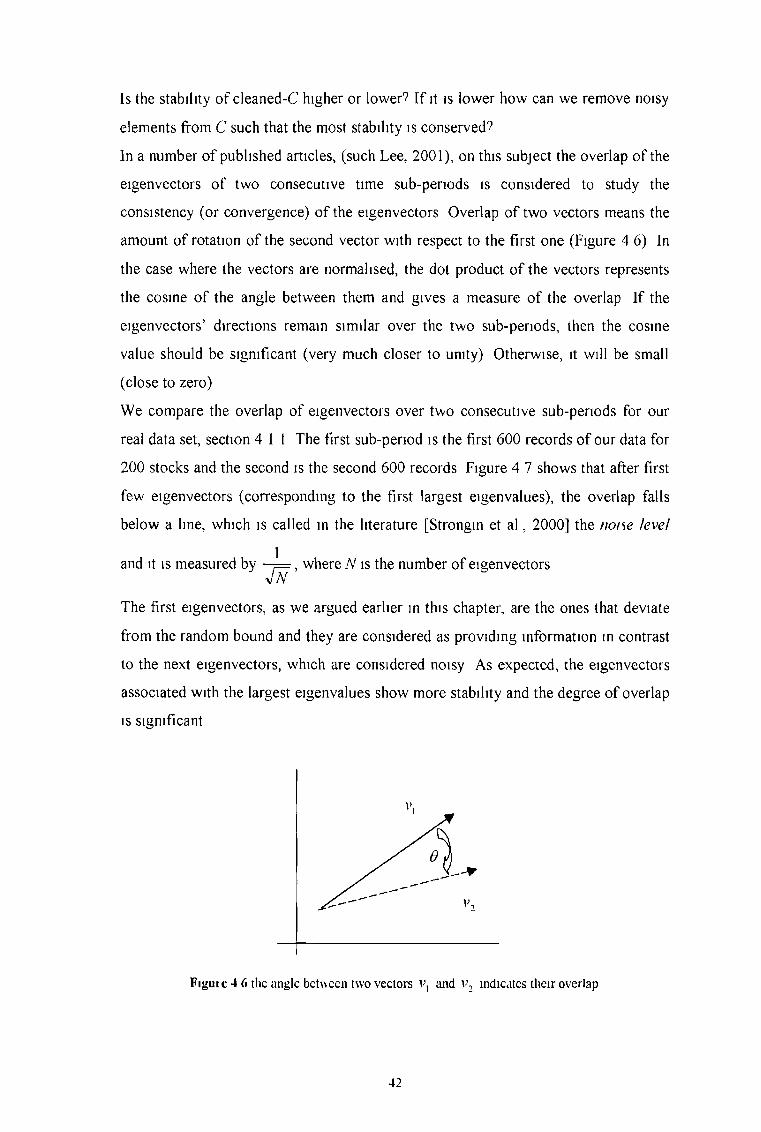
In a number of published articles, (such Lee, 2001), on this subject the overlap of the
eigenvectors of two consecutive time sub-periods is considered to study the
consistency (or convergence) of the eigenvectors Overlap of two vectors means the
amount of rotation of the second vector with respect to the first one (Figure 4 6) In
the case where the vectors are normalised, the dot product of the vectors represents
the cosine of the angle between them and gives a measure of the overlap If the
eigenvectors’ directions remain similar over the two sub-periods, then the cosine
value should be significant (very much closer to unity) Otherwise, it will be small
(close to zero)
We compare the overlap of eigenvectors over two consecutive sub-periods for our
real data set, section 4 1 1 The first sub-period is the first 600 records of our data for
200 stocks and the second is the second 600 records Figure 4 7 shows that after first
few eigenvectors (corresponding to the first largest eigenvalues), the overlap falls
below a line, which is called in the literature [Strongin et a l , 2000] the noise level
and it is measured by ■—= , where N is the number of eigenvectors
The first eigenvectors, as we argued earlier in this chapter, are the ones that deviate
from the random bound and they are considered as providing information in contrast
to the next eigenvectors, which are considered noisy As expected, the eigenvectors
associated with the largest eigenvalues show more stability and the degree of overlap
is significant
Figuic 4 6 the angle between two vectors and v2 indicates their overlap
42

Figure 4.7 Eigenvector overlap between the two sub-periods. The horizontal line is the noise level
However, to measure more formally the stability of a matrix and its eigenvectors, we
employ another approach in the literature on principal components suggested by
Krzanowski (1984). Krzanowski (1984) examines the effect on vk (k111 eigenvector)
of small changes in the value of Xk (kth eigenvalue) and he argues that this is
important because it gives information on the stability of the principal components.
The principal components can only be securely interpreted if they are stable with
respect to small changes in the values of the Xk ’s. Specifically, he investigates the
perturbation of an eigenvector derived for a small reduce/ increase, £ , in the
corresponding eigenvalues. He determines the component, v(i), which diverges as
much as possible from the ith eigenvector, v-, but whose eigenvalue is at most €
greater/ less than that of v., such that the angle 6 between v(i) and v, can be
calculated by equation (4.7).
43

C O S # ~ ^ (4 7)
n + ---------- )~1/2 i f s iS increased to X; 2 1 A,-i ~ A,
(1 + ---- ----- ) 1/2 if s is decreased from Xx
where X] > X2 > > Xn This equation demonstrates that the effect on vf of an e
change in Xt is an inverse function of X} ~ Al+] Thus it is not the absolute size of the
eigenvalue which determines whether that component is stable or not but rather its
separation in terms of eigenvalue from the next component Relatively isolated
(early) components with large eigenvalues should therefore be fairly stable, but later
components all of which have similar non-zero variances will not be stable So the
largest non-zero eigenvalue and corresponding eigenvector can be used to find the
smallest perturbation in vr which leads to a change s in Xx
4 2 1 Stability of the correlation matrix
In this section we study the stability of C for our real data using the Krzanowski’s
model [Krzanowski, 1984] in equation 4 7 The angle between eigenvector i of
original C and v(i) is calculated, where v(i) is the perturbation of /th eigenvector
derived for a small change in Xx (Figure 4 8) Also l is determined by the empirical
changes in the average of Xx from the first sub period to the second sub period It
approximates to 0 2% in our experiments So, effectively a perturbation method is
implied
44

Cosine 9
Figure 4 8 Cosine 9 for eigenvectors of original correlation matrix where 9 represents the perturbation of vt derived for the change of 0 2 % in A}
As expected, Figure 4 8 shows that the first (largest) eigenvectors are the most stable
ones (<cos 9 large) Also the last (smallest) eigenvectors show higher stability than the
middle ones, which is because the smallest eigenvalues approach zero and therefore
in Equation 4 7, cos 9 represents greater values
Examining figure 4 3(a) again one can see that the top end of the predicted and
realised curves are further apart whereas the bottom and the middle area are closer
(about 19% of the top distance) Since the area of the efficient frontier associated
with the highest risk, is corresponding to the largest eigenvalues, and the largest ones
are the most stable ones, then we can conclude that as stability gets progressively
lower the curves gets progressively closer This contradicts the conclusion of
Bouchaud et al (2000) They attribute the closeness of the mentioned curves to the
higher stability whereas we conclude that it is due to reduction in stability We now
discuss this in greater detail
45

4.2.2 Stability of the cleaned correlation matrix
According to Equation 4.7 we examine the stability of cleaned_C where the method
of Bouchaud et al (2000) is used for cleaning (Figure 4.9).
Cosine 6
Figure 4.9 cosine 6 for eigenvectors of original C (solid blue curve) and cleaned_C (dashed red curve) where 6 represents the perturbation of V, derived for the change of 0.2 % in .
It can be seen from the Figure 4.9 that the stability of the eigenvectors of cleaned_C
has declined noticeably to a low point after the 11th eigenvector (the edge of the
noisy/ non-noisy determined of RMT prediction).
That happens because the noisy band of eigenvalues is replaced by their average,
which means no separations between the eigenvalues at all.
Also Figure 4.9 (in contrast to Figure 4.3b) again illustrates the negative relationship
between stability of eigenvectors (and therefore C) and the distance between two
predicted and realised curves. As the stability decreases, the two curves get closer
and conversely when stability increases the distance between curves gets larger.
46

4 3 A n e w a p p ro a ch to m a tr ix f i l t e r in g
We propose a new method of filtering C to preserve the stability of the matrix as
much as possible The principle is to replace the noisy eigenvalues with components
that have most separation from each other, while maintaining a fixed sum (according
to Equation 4 3, the sum of eigenvalues should be constant) In Figure 4 10 the noisy
part of the graph is changed to an oblique line The slope is determined so that on
one hand the most separation between components is attained and on the other hand
none of the eigenvalues is replaced by negative values (as all the eigenvalues of the
correlation matrix are positive)
To have an idea of how the method works, Figure 4 11 shows the eigenvalues of filtered_C
(or cleaned_C)
Eigenvalue
2
1 8
1 6
1 A
1 2
1
0 8
0 6
0 4
02
020 40 60 80 100 120 140 160 180 200
Figure 4 10 Replacement of eigenvalues The non-noisy largest values are untouched, but other parts have been replaced such that each two ones arc kept in the most distance
47

Eigenvalue
Figure 4 11 Eigenvalues of filtered_C Eigenvalue after 11th oscillate since each two ones are kept inthe most distance as possible
To observe the stability of this new filtered_C we compute its cosO (in Equation
4 7) This is shown in Figure 4 12 As can be seen the stability of noisy eigenvectors
of the original matrix is higher than those of the filtered matrix up to approximately
150th eigenvector and it is lower after 150th Thus, this method keeps stability much
higher in comparison with the flattening of the eigenvalues, (the method of
Bouchaud et al (2000)) Concerning the previous results from section 4 2 1, we
expect that the predicted and realised risk-return curves are closer on graph in the
interval between 11th to 150th and farther apart after 150th in comparison to those of
original C
48

Cosine 6
Figure 4.12 Cosine 6 for the original matrix C (solid line) and filtered-C by the method based onKrzanowski results (dashed line)
Again the largest eigenvalues correspond to the riskiest portfolios exposed in the top
area of the efficient frontier in Figure 4.13. Equally the smallest eigenvalues
correspond to the least risky portfolios, exposed in the lower area. As can be seen,
the upper end, d^lt, of the curves in Figure 4.13 converge whereas the middle parts,
d{H*, are less close than those for original_C. This is another indication of the
validity of our assertion that stability has an inverse relation to the distance between
the predicted and realised risks. As the stability gets higher the closeness between
curves decreases and vice versa. If d™g stands for the distance between the upper
end of the curves for original_C, and d°^R for those of middle parts, then we have
found that:
Table 4.1 % Closeness of curves
¿ r = 6 3 % c
¿¿ f '= 68% d f*
49

We conclude from these findings is that the method of cleaning C suggested by
Bouchaud et al (2000) has a detrimental impact on the stability of C. Furthermore,
the closeness of the predicted and realised curves does not necessarily represent the
power of prediction of risk in future. Indeed, when the correlation matrix is less
stable, the predicted and realised curves are closer than the case with more stability.
(a) Risk
Figure 4.13 (a) Portfolio return versus risk for the family of optimal portfolios constructed from the original matrix C (red and blue curves) and filtered_C (triangle-green and circle-magenta curves).
50

0.025 0.03 0.035 0.04 0.045(c ) Risk
(Continued from last page.) (b) A closer look at the top of the graph of (a); d/jlt is smaller than
d y ,g (c) The closer look at the bottom area of the graph (a); d ^ lg is smaller than d ̂ lt.
51

4 4 C o n c lu s io n
In this chapter we have examined the principally-used technique of noise removal for
the correlation matrix, C This technique, which proposes flattening the noisy part of
the eigenvalues, largely decreases the level of stability of C We have applied
Krzanowski’s stability model to study the stability of the financial correlation matrix
after removing the noise According to this model, we have discovered that the
advocated technique for noise removal destroys the stability of C
Based on the Krzanowski’s model we proposed a novel technique to filter C such
that the stability of the matrix is preserved This model keeps the noisy eigenvalues
at maximum separation from each other while the trace of C is kept the same
To see the effect of noise removal, Bouchaud et al (2000) have suggested comparing
the realised and the predicted optimal portfolios They have found a shorter distance
between the realised risk and the predicted risk for the cleaned_C than that of the
original C They have attributed this as a higher stability of the cleaned_C
In our study we have shown on a set of itra-day data from S&P500 that this is not the
case and in fact there is a negative relationship between the stability of C and the
closeness of the predicted and realised risks This assertion is also demonstrated
through experiments of filtering C based on the Krzanowski’s model Therefore the
common technique of noise removal not only does not promote the stability and
hence power of prediction, but actually leads to a noticeable deterioration and should
be avoided
52

Chapter 5 E p o c h s
This chapter is about co-movement among stocks as influenced by market price
changes We propose a new approach to study market reaction to high volatility and
use the Spectral Theorem [Strang, 1988] to measure the day-to-day co-movement of
stocks A new concept of epochs is introduced where these represent patterns defined
in terms of daily change m the largest eigenvalue and daily change in market sector
prices The evidence suggests a strong linear relationship between price and the
largest eigenvalue in the epochs but the error terms m the linear models show
correlated behaviour Therefore, a modified model is introduced Further, some break
points are observed in the modified model, for which we discuss possible reasons
53

5 1 V o la t i l i t y
After the crash of October 1987, few people would argue that stock market volatility
changes randomly over time Researchers (beginning with Black (1976)) have found
evidence that stock prices are negatively correlated with volatility A price drop
increases the risk of a company going bankrupt, and its stock therefore becomes
more volatile It is also said, [Nelson, 1991], that volatility tends to rise in response
to bad news and to fall in response to good news The economic reason for this is
unclear Although it has been long understood [Christie, 1982] that financial leverage
plays a role, it has not been possible to explain the extent of the asymmetric response
of volatility to large sudden positive and negative returns
What is known is that large negative stock returns are more common than large
positive ones, so stock returns are negatively skewed (For example, according to an
investigation by [Cutler et a l , 1989], 8 out of 10 largest movements in the S&P500
have involved declines since World War 2, and only two have increased )
However, we have found work [Black, 1976][Chnstie, 1982][Campbell et a l ,
1992][Bekaert et a l , 2000] on volatility and crashes to be reticent on the effect of
price changes on “market movements” What we mean by “market movement” is
combined upward or downward behaviour of stocks This is the quantity measured
by the largest eigenvalue of the covariance matrix1 made up of the stocks prices/
price changes [Alexander, 2001]
Regarding chapter 3 and 4, we know that the largest eigenvalue of the covariance
matrix is the most “reliable” eigenvalue, 1 e the most deviated one from the noise
band Therefore, although the covariance matrix contains much noise, the largest
eigenvalue appears to contain true information about correlated movements of stocks
and, unlike other eigenvalues, all the analyses depending on that are likely to be
adequate In this study we propose a novel approach to risk recognition (or risk
response) The suggested method is based on measuring the day-to-day changes of
the riskiest position on stock combinations, which is determined by the largest
eigenvalue of the covariance matrix
1 It should be mentioned that the covariance and correlation matrices are most of the time used interchangeably They have the same properties except that the correlation matrix removes the variances by normalisation
54

5 1 1 R is k
Investors should not and indeed do not hold a single asset (or even asset class)
Holding a multiple-asset portfolio, on the other hand, makes returns on assets
‘uncertain’, since two assets yielding different ‘certain’ returns cannot both be
available (as everyone will want to invest in the higher yielding asset and no one will
purchase the lower yielding one) If everyone knew with certainty the returns on all
assets, then a general framework for a rational portfolio selection could be
introduced In the case of common stocks it is impossible to predict the value of
portfolio at any future date The best an investor can do is guess the most likely
estimates In this case, it is said that the investor bears risk In order not to incur risk,
an investor might hold a portfolio of Treasury Bills, and of course, face no
uncertainty, because the value of the portfolio at the maturity of the securities will be
identical with the predicted value In the literature review earlier, we explained that
variance (or standard deviation) of return is the most common feature to measure the
risk From Markowitz diversification [Markowitz, 1991], the variance (and hence
overall risk) of a combination of two assets can be even less than the variance of
either of the assets, themselves This is because the risk of a combination of assets is
calculated from equation 2 1 For the case when the portfolio of assets is equally
weighted, the equation 2 1 can reduce to
<JN
+ <j . (5 1)
(where bar notation denotes a time average and N is the number of assets ) Hence,
when the number of assets gets large enough, the variance of a selection of assets
depends only on the average of the covariances between stocks To calculate the
covariance between assets price/ price change, similar to the previous chapters we
have
= G .(0 G ,(0 . (5 2)
55

(where G; represents assets price or price change (dependent on what is used in
practice) and the bar denotes a time average over the period studied) In matrix
notation the covariance matrix can be calculated as following,
C ' = j G G T, (5 3)
(where G is an N x T matrix with elements G, (t) , j=l3 ,N, t=l, ,T )
It should be mentioned that the matrix of the assets time series, G, is not normalised
with respect to the variance as in Equation 3 1 The normalisation process includes
removing the volatility information on co-movements of stocks, which is not
particularly useful for our experiments here since we aim to study the volatility
behaviour itself Therefore, the covariance matrix that we construct is not a
normalised covariance matrix
5 2 M ethodology
From the spectral theorem we know that any N x N symmetric matrix can be
decomposed into
i=iN (5 4)
= ' L à>p .
(where p t = vtv^ , the outer product of the eigenvectors) Since the covariance matrix
is symmetric, therefore spectral decomposition can be used, 1 e
(5 5)1=1
Hence, the N * N covariance matrix is decomposed into a product of its eigenvalues
and eigenvectors
56

Our suggested method to measure the day-to-day variation of co-movements of
stocks is to take the difference between the two covariance matrices corresponding to
two consecutive days/ observations and examine the effect on the maximum
eigenvalue It means that if C 'm represents the covariance matrix corresponding to m
recent days ( 1 e an average based on a window of m days) and C*m+\ represents the
covariance matrix corresponding to days, then the difference between C #«+i
and C*m will be the covariance matrix on day m-\ 1 With respect to the spectral
theorem we can write
- C \ = J A ; +V r W (5 6)»=] 1 = 1
= i - c v r 1 - ¿ w +l + i » r ' - I k p : (s t>l-l 1=1 !=1 (=1
= £ ( ¿ r 1 - a;- ) / r +l + £ ̂ cp,m+l - Pr ) (5 s)1 = 1 ¡=i
Equation 5 8 clearly shows how the daily variation of prices can be reflected in the
daily variation of the eigenvalues of the covariance matrix As we have mentioned
earlier m this chapter, our analysis focuses on the most reliable eigenvalue, which
contains information about the co-operation of the stocks Also, for more
convenience, the study of - A™, where i gets values from 1 to N, can be replaced
by the study of —̂ ( s h o w n in appendix A)K
To our belief use of the daily changes of the largest eigenvalue as a barometer of the
'risk perception’ by the market is a novel approach We define these changes of the
maximum eigenvalues as the change in cohesion As the largest eigenvalue reflects
the high level of coherent trading activity in the market, we consider the degree ofjT-rl
uniformity in response to the coherence Therefore, in our study is recognised"̂ max
as the change in cohesion with time and is denoted lsCohT
57

5 3 E xperim ental results
5 3 1 Epochs Definition
The data set we use for this part, is daily market sector prices from the Dow Jones
EURO STOXX2 over a time period started from the first of January 1996 to the first
of October 2002 This data set is divided into different market sectors allowing us to
examine change m cohesion for each
First, we take an initial time window of one year (i e 260 days) and step-by-step
move on to construct the covariance matrices on each day using Equation 5 3 Next,
calculating the change in cohesion (as mentioned by the ratio of consecutive
maximum eigenvalues) over consecutive time periods, we plot it versus the price for
each market sector index Figure 5 1 shows the daily change in cohesion against
price for Technology, Telecom, and Industry indices An interesting result is the
linear relationships between the price index and the change in cohesions, which may
be clearly observed Also additional patterns are seen in plots, which seem to show
how the market is organising itself We call these growth patterns “epochs” Epochs
are the focus of our discussion here, and we will characterise them and seek to
explain their occurrence
2 http //www stoxx com
58

Price
Pr
ice
1400
1200
1000
800
600
400
200
00.998 1 1.002 1.004 1.006 1.008 1.01 1.012 1.014 1.016
Change in Cohesion
(a)
1100
1000
900
800
700
600
500
400
300
200
1000.998 1 1.002 1.004 1.006 1.008 1.01 1.012 1.014 1.016
Change in Cohesion
(b)Figure 5.1 epochs skeleton for (a) Technology, (b) Telecom, and (c) Industry
ca

4 0 0
3 5 0
3 0 0
o. g 2 5 0
cl
200
1 5 0
1000 . 9 9 8 1 1 . 0 0 2 1 . 0 0 4 1 . 0 0 6 1 . 0 0 8 1 . 0 1 1 . 0 1 2 1 . 0 1 4 1 . 0 1 6
Change in Cohesion
( c )
(continued from the last page).
5.3.2 Epochs: Discussion
The linear relationship between price changes and the cohesion degree changes of
particular points, where the coherence appears to return to a lower value at the end of
each epoch. In addition, it seems that epochs are characterised by progressively
higher slopes until this expansion or inflation can no longer be maintained in the
prices. This also supports the indecisive parts of the end of the epochs, which tend to
happen after a period of maximum prices and for which no higher degree of cohesion
can be observed.
For a better understanding of this phenomenon, it is instructive to pinpoint the
turning point/ end of each epoch. For this purpose, we measure the statistics of the
progressive regression fits. If linear fits start from a couple of points at the beginning
of data and move toward the next point every time, there should appear a sharp drop
in the value of R-Squared3 at a particular point. We consider this sudden fall as the
turning point of each epoch. In fact the progressive fits continue to maintain a stable
3 A measure of how good a fit is.
450
60

or constant value until the point where the relationship between price and cohesion
changes and the model fits start to diminish. As a measure of how good a model fit
is, we use the R-Squared statistic. Therefore, by looking at the progressive R-
Squared values we determine where the model fits tend to fall. Before getting to the
turning point, the values of R-Squared tend to improve and in some stages they show
stabilising behaviour (i.e. getting to a consistent value of R-Squared). As they get to
a turning point, a sudden drop in the R-Squared value is observed. Figure 5.2 shows
the change of R-Squared for one of the epochs observed in Figure 5.1(a). Before the
40th point (Figure 5.2), an improvement in the model fits is observed but at 40th point
a sudden drop occurred. This point is associated with the date of 14/09/1998, which
we believe should be one of the key turning points. Some of these identified points
are presented in Table 5.1. In order to determine what happened on these days we
searched the archive of newspapers or weekly news such as ‘Guardian’, ‘Irish
Times’, and ‘Business Week’. The results of that are shown in Table 5.1. For
example the date of 14/09/1998 is corresponding to the ‘global crisis’ when markets
all around the world were in decline due to the Asian Crisis.
Days
Figure 5.2 Progressive R-Squared values corresponding to the Technology- Cohesion graph. A sudden drop on the point of 40th day is observed.
61

1400.
1200n
Cohesion Change
Figure 5.3 The time dependence of epochs for Technology plot
It should be mentioned, however, that some of the epochs are very volatile and
identifying an exact turning point is sometimes difficult. In addition, the identified
points in a few cases are not consistent with what one sees. This appears to be the
case mostly in the epoch with the largest slope. What one sees is different from what
theory describes (Table 5.1). But if we plot a 3-dimension graph of epochs, where a
time dimension is added to the two other dimensions, it could be easier to distinguish
the turning points of epochs. Figure 5.3 shows the 3-dimensional plot of figure
5.1(a), when the time axis is the third dimension.
However, the model fits should be specified and its parameters estimated, while
assumptions and conditions underlying the model should be explored. As each epoch
is identified earlier data should be dropped to identify the next one.
62

Table 5 1 The identified turning points of epochs corresponding to key events in the market
Date Event
06/02/1996 Apple Computer in decline
17/03/1997 Fall of Dow Jones after the Warren Buffet’s speech, UK pre-election
period
31/07/1997 European markets fell sharply, worrying about the Greenspan report to
Congress
29/08/1997 Fears of higher German interest rates
20/04/1998 Microsoft fear of splitting
20/07/1998 European markets fall Japanese and Russian economic crisis
14/09/1998 Global crisis due to Asian crisis
25/05/1999 China-US relationship crisis
23/07/1999 Market slump after Greenspan address
14/10/1999 Inflation, interest rate rise fear and a warning from Greenspan
24/04/2000 Backlash behind the anxiety over Globalisation
01/05/2000 Fall of Dot-com
12/12/2000 US Supreme Court Judgment Ratifies President Bush
18/12/2000 Tech slump
28/03/2001 Cut in Federal Reserve rate
11/09/2001 September 11th
02/07/2002 Scandal in Worldcom unfolding
12/07/2002 European markets tumbled after the SAP-Deutschland warning
5 3 3 Epochs Models
Cohesion graphs in Figure 5 1 appear to be characterised by periods of linear
regression fits between price and change in cohesion The linear regression model is
of the form
Yt =at X t +bt +et (5 9)
(where Yt is the daily price, X t is the daily change in cohesion, s t is a random error
term with zero mean and at and bt are regression coefficients, both functions of
63

time) In this model, the random errors should be independently distributed 1 e
cov{e( , s t }=0 for all i, j, i * j [Neter et a l , 1990] To test for independence of
error in the regression model, it is usually suggested [Neter et a l , 1990] to prepare a
time plot of residuals The purpose of plotting residuals versus time is to see if there
is any auto-correlation between the error terms over time If a trend can be seen in
the residuals, it is concluded that the errors are non-independent, otherwise they are
presumed to be independent Therefore, we need to calculate and plot the residuals of
our model over time Figure 5 4 shows two samples of these plots calculated from
06/02/1996 to 17/03/1997 and the other from 29/08/1997 to 20/04/1998 It should be
mentioned that these four dates are obtained from Table 5 1
From Figure 5 4 it is evident that there is a correlation between the error terms
Negative residuals are associated mainly with the early trails, and positive residuals
with the later trails4 It clearly can be observed that there is a trend in Figure 5 4 (a)
and (b) This means, therefore, that s t are not independent Although we have got
good fits (R_Squared values between 0 45- 0 66) for most market sectors, the
dependency of error terms is against the model’s assumptions and, therefore, should
be eliminated In this case, a transformation that is often helpful to remedy such
dependence is to work with first differences of the model Hence, we take the first
differences of the Equation 5 9
Y ^ y X ’t + p + S i t X y (5 10)
(where /? is found to be typically small and positive and y , 8 are large and
negative, positive respectively)
The Durbin-Watson5 (DW) test is then applied to test whether the error terms for the
transformed model are uncorrelated We re-examine the transformed model and find
that the DW statistic is satisfied with the values very much close to 2 Therefore,
there are no more patterns in the residuals left (white noise) However, the regression
4 When the error term arc independent it is expected that the residuals fluctuate in a more random pattern around the base line zero5 It is a test for serially correlated (or autocorrelated) residuals If the residuals are uncorrelated, the expectcd DW statistic is 2
64

model shows poorer fit with the R-Squared values smaller after modifying the
regression model.
5.3.4 Sampling rate analysis
We tried to examine different sampling rates other than daily rates to see the effect of
differencing on the lower sampling rates. Two days, 5 days, 10 days and monthly
sampling rates are tested. Table 5.2 represents the reduction of the R-Squared for the
Technology market sector index. As can be seen, DW statistics were obtained for a
variety of granularities.
50
40
30
20w« 10 3
-gC/)Q) 0 CC
-10
-20
-30
-4006/02/1996 25/06/1996 12/11/1996 17/03/1997Date
(a)Figure 5.4 Residual- time plots illustrating nonindependence of error terms, (a) The residuals associated with the model fitted over the period from 06/02/1996 to 17/03/1997 and (b) from
29/08/1997 to 20/04/1998.
65

50
40
30
20wCO D-q 1 0 w © cc
0
-10
-20
-3029/08/1997 21/11/1997 16/02/1998 20/04/1998
Date
(b)
(continued from the last page)
Table 5.2 Model fit statistic for technology at different sampling rates
Sampling Rate R-Squared DW Statistic
Monthly 0.46 1.97
Every 10 Days 0.40 2.05
Every 5 Days 0.40 2.20
Every 2 Days 0.20 2.05
What can be seen in Table 5.2 is that the goodness of fit is reduced for the higher
resolution data. This might suggest that there exists a high volatility in data, which
induces the poor fit for higher sampling rates. In other words, although at daily rates,
modifying the model results satisfactorily in white noise, the prediction power of the
modified model is poorer.
The model failure for fine granularity is discussed in the following section.
5.4 Possib le reasons for m odel failure
Possible reasons for regression model breakdown can be:
66

1 Day of the week, which means that market behavior on particular days of the
week, is reflecting the different level of activities affected by closing, starting or
mid-week time
2 Outliers, which means that large price changes, are only reflected in the high
resolution data
The first case can be rejected because the eigenvalue changes show high variability
on all days of the week, and there is distinctive pattern for variability over particular
days The second one is refuted too, since the model fits are satisfactory for lower
resolution though not for higher ones Also the epoch skeleton can be observed for
all the sampling rates including the monthly case (Figure 5 5)
Furthermore, outlying points seem to have little effect on the R-Squared and DW
statistic, as their number is very small compared to the overall number of
observations
Change in Cohesion
Figure 5 5 Epoch skeleton for monthly sampling rate is retained
Finally, there exist some periods (of a few-days-length) in the market data, which
reflect the failure of the general model fits Clearly, these periods, where the short
term volatility increases, are associated with changes in cohesion As we explained in
67

the previous sections ^ ax could be considered as a measure of volatility and
therefore, the change in cohesion ACohT is interpreted as the proportional change in
volatility This high volatility naturally represents ‘short-term7 lack of co-operative
behaviour Since coherence describes the change in common perception of risk, lack
of common perception provides fluctuations over the short-term and this reduces the
goodness of fit In the epoch plots, the coherence (or co-operative behaviour in
market trading) is clearly lower at the end of epochs, which is due to the lack of
common perception of risk However, it is suggested that the breakdown in
coherence can be used as a measure of critical market uncertainty
5 5 C onclusion
In this chapter we introduced the concept of cohesion, which is co-operative
behaviour in market trading and also demonstrated the existence of epochs or growth
patterns in the Dow Jones Euro STOXX market sector Epochs represent the linear
relationship between the sector price change and the daily change in cohesion They
are defined in all market sectors but can be observed more strongly in Technology,
Telecom and Industry (less so in “defensive” sectors such as Food or Automobile)
The end of each epoch, where the coherence or cohesion has returned to a lower
value, represents a relatively critical situation in the market However, the existence
of high volatility, which is naturally dominant over short-term periods, diminishes
the power of predictability of sustained changes
68

Chapter 6C o n c lu s io n s a n d F u tu re w o r k
The overall goal of this thesis was to study the risk and co-movements of financial
stocks We have studied the role of the correlation matrix in order to determine the
risk on a set of assets The major theories in finance are based on a true measure of
correlations among assets We have shown that the so-called historical correlation
matrix, C, contains a large amount noise and we applied the theory of random
matrices to determine the noise in C For a set of actual data from S&P500 we
realised that approximately 95% of eigenvalues of C do not contain true information
This is supported to some extent by other work [Plerou et a l , 1999][Laloux et a l ,
1999], which considers that at most 6% of C carries useful information The noise
involved in C is due to the finite number of records and the non-stationary
correlations between stock prices We also performed an eigenvector analysis m
69

complement to the correlation matrix analysis, where we expect that the eigenvector
corresponding to the maximum eigenvalue has a different construction from those
representing true information
In order to see the result of RMT on different volumes of noise involved in financial
data, we presented simulations creating a sinusoidal time series By adding different
volumes of random noise controlled by the amount of standard deviation, different
noise volumes in time series were studied and RMT applied to each The evidence
suggests that the number of deviated eigenvalues from the random bound does not in
general depend on the volume of the added noise All volumes of noise examined
gave approximately the same number of deviated eigenvalues These were associated
with the non-noisy part of C and the value of RMT here would appear to be in
distinguishing the non-noisy or information-rich values
After applying RMT and identifying the amount of noise in C, some techniques are
needed to separate and remove the information from the noise We used the principal
technique of noise removal [Laloux et a l , 2000], which proposed flattening the noisy
part of the eigenvalues However, in examination of the stability of the matrix after
noise was removed, we concluded that the standard method may actually destroy
stability On the basis of results for stability obtained from the Krzanowski’s stability
model, we therefore proposed a technique to filter C such that the stability of the
matrix is preserved This model keeps the noisy eigenvalues at maximum separation
from each other while the trace of C is kept the same
To test the effects of noise removal, Bouchaud et al (2000) have suggested
comparing the realised and the predicted optimal portfolios They have found a
shorter distance between the realised risk and the predicted risk for the cleaned_C
than that of the original C They have attributed this to higher stability of the
cleanedC
In our study we have demonstrated that this is not the case and, in fact, there is a
negative relationship between the stability of C and the closeness of the predicted
and realised risks This assertion is also showen by experiments in filtering C based
on Krzanowski’s model We conclude therefore that the common technique of noise
removal not only does not promote the stability and therefore the power of
prediction, but actually leads to some deterioration
70

• A p ra c tic a l a p p lic a t io n fo r th e re s u lt o f R M T
With respect to principal component analysis, we know that the minimum eigenvalue
of the correlation matrix is associated with the least risky position on a stocks
combination and the maximum eigenvalue is associated with the most risky position
The result from RMT tells us that the combination of assets corresponding to the
most risky position is the most reliable one Therefore, unlike for minimum
eigenvalues, analyses dependent on the maximum eigenvalue are likely to be
adequate
By studying the daily changes of the riskiest position on stocks combinations, we
have aimed to study the market risk behaviour New concepts of ‘cohesion\ and
cepochs' have been introduced We have demonstrated the existence of epochs in
EURO-STOXX market sector data, for which linear relationships between change in
cohesion and market sector prices are observed The end of each epoch, sees a fall in
coherence representing a relatively critical situation in the market The evidence
supports a relationship between volatility and the change in the cohesion, but
volatility is naturally dependent on short-time periods and therefore the existence of
high volatility, diminishes the predictability of the model fits
As a final note, it is suggested that coherence provides a measure that can be directly
linked to critical market uncertainty
• F u tu re w o rk
Some analysts would claim that noise is a reflection of the various trading strategies
of the investors in the market [Long et a l , 1990] In order to estimate the causes of
noise, we have considered the use of fractional calculus, (which deals with
applications of integral/ derivatives of arbitrary order) The recent application of
fractional calculus model in finance has provided the modelling of non-Gaussian
probability distributions, as are found in financial data where large fluctuations are to
be expected In the case of the correlation matrix, application of the fractional
calculus model will draw on more detailed analysis of the statistical feature of nsk-
71

return on combination of assets in relation to time-dependent behaviour of the
eigenvalues, which reflect stock movements
72

G lossary
P the ratio of covariance between stock’s return and market’s return to the
variance (or volatility) of the market
Broker an individual or firm, which facilitates a deal between a buyer and seller
Change in cohesion the change of the maximum eigenvalue
Cleaned correlation matrix the correlation matrix re-constructed after removing
noise also expressed as cleaned_C
Co-operative behaviour the common understanding of selling/ buying stocks in a
market
Derivatives Derivative (or derivative security) is a financial instrument whose value
depends on the values of another asset
Dividend taxable payments declared by a company’ s board of managers given to its
shareholders out of the earning of the company at the present Usually quarterly and
given as cash
Efficient frontier the line on a nsk-return graph comprised of all optimal portfolios
Epochs progressive patterns defined in terms of daily change in the largest
eigenvalue and daily change in market sector prices
Financial assets financial assets are instruments to claim amount of cash at some
future time The price of a financial asset equals the present value of all cash
dividends that the asset provides its owners
Indicator a statistical construct that measures price changes and/ or returns in stock
market
Liquidity the ability of an asset to be converted into cash quickly
Listed stock Stocks that are traded on an exchange are said to be listed stocks
Market value the value of a company’s outstanding shares, as measured by shares
times the current price Also known as market capitalisation
Optimal portfolio a portfolio that provides the greatest expected return for a given
level of risk, or equivalently, the lowest risk for a given expected return, also called
efficient portfolio
Price change the difference between asset’s values on two consecutive days
73

Rate of return the annual rate of return on an asset expressed as a percentage of the
total amount invested, also called return
Return return for a particular time period is equal to the sum of the price change
divided by the price at the beginning of the time period
74

R eferen ces
Alexander, C (2001), Market models A guide to financial data analysis, John
Wiley & Sons
Bekaert, G and Wu, G (2000), Asymmetric volatility and risk in equity markets,
The review of financial studies, 13(1), 1-42
Bibby, J (1980), Some effects of rounding optimal estimates, Sankhya B , 42,
165-178
Black, F (1976), Studies of stock market volatility changes, Proceedings of the
American statistical association business and economic, 177-181
Blume, M E (1970), Portfolio theory a step toward its practical application,
Journal of Business, 152-173
Bouchaud, J P and Potters, M (2000), Theory of financial risk, Cambridge
University Press
Business week online (2003a),
http //www businessweek com/magazine/content/03_10/b3823013_mz001 htm
Business week online (2003b),
http //www businessweek com/magazine/content/03_10/b3823001_mz001 htm
Business week online (2003c),
http //www businessweek com/magazine/content/03_10/b3823015_mz001 htm
Campbell, J Y and Hentschel, L (1992), No news is good news An asymmetric
model of changing volatility in stock returns, Journal offinancial Economics, 31,
281-318
75

Chan, L K C , Karceski, J , and Lakomshok, J (1999), On portfolio optimization
forecasting covariances and choosing the risk model, Review of Financial
Studies, 12(5), 937-974
Chance, D M (1995), An introduction to derivatives, Dryden press
Christie, A A (1982), The stochastic behaviour of common stock variances
value, leverage and interest rate effects, Journal of financial economic, 10, 407-
432
Crane, M , Keogh, G , Ruskin, H , and Sharifi, S (2002), Leverage and cross
asset volatility correlation- Empirical or optimistic, Nikkei conference
proceeding
Cutler, D , Poterba, J M , and summers, L H (1989), What moves stocks prices,
Journal of portfolio management, 15(3), 4-12
Dyson, F J (1962), A browman-motion model for the eigenvalues of a random
matrix, Journal of mathematical physics, 3(6), 1191-1198
Dyson, F J , and Mehta, M L (1963), Statistical theory of the energy levels of
complex systems, Journal of mathematical physics, 4, 701-712
Dyson, F J (1971), Distribution of eigenvalues for a class of real symmetric
matrices Revista Mexicana de fisica , 20, 231-237
Edelman, A (1988), Eigenvalues and condition numbers of random matrices,
SIAM Journal on Matrix Analysis and Applications, 9, 543
Elton, E , and Grouber, M (1973), Estimating the dependence structure of share
pnces-Implications for portfolio selection, Journal of finance, No 5, 1203-1232
Elton, E , Gruber, M and Unch, T (1978), Are betas best?, Journal of finance,
23(5), 1375-1384
76

Elton, E , and Gruber, M (1981), Modern portfolio theory and investment
analysis, John Wiley & Sons Inc
Fabozzi, F J , Modigliani, F , and Fern, M G (1998), Foundations of financial
markets and institutions, prentice-Hall Inc
Facts on file news services (2002), http //www facts com/
FTSE web site (2003),
http //www ftse com/indices_marketdata/uk_series/index_home jsp#ftseI00
Fuller, R J , and Farrell, J L (1987), Modern investments and security analysis,
McGraw-Hill
Graham, B , Dodd, D and Cottle, S (1962), Security analysis, McGraw-Hill
Green, B F (1977), Parameter sensitivity in multivariate methods, I Multiv
Behav Res , 12, 263-287
Guardian Century (2003),
http //www guardiancenturv co uk/1980-1989/Story/0.6051.110247,00 html
Hull, J (2000), Options, futures, and other derivatives, Prentice Hall
Investors glossary on the web (2003), http //www investorwords com
Jolliffe, I T (1986), Principal component analysis, Springer-Verlag
Jolhffe, I T , and Stephenson, D B (2003), Forecast Verification A Practitioner’s
Guide in Atmospheric Science, lohn Wiley & Sons
Keogh, G , Sharifi, S , Ruskin, H , and Crane, M (2003), Epochs in market
sector index data- empirical or optimistic, to appear in Lecture Notes in
Computer Science, Springer-Verlag
11

Kim, J , and Mueller, CW (1979), Factor Analysis Statistical Methods and
Practical Issues, Sage Publications
King, B (1966), Market and industry factors in stock price behaviour, Journal of
business, 39, 139-140
Krzanowski, W J (1984), Sensitivity of principal components, Journal of royal
statistics society B, 46(3), 558-563
Laloux, L , Cizeau, P , Bouchaud, J P , and Potters, M (1999), Noise dressing of
financial correlation matrices, Physical Review Letters, 83(7)
Laloux, L , Cizeau, P , Potters, M , and Bouchaud, J P (2000), Random matrix
theory and financial correlations, International journal of theoretical and applied
finance, 3(3), 391-397
Lee, Y H (2001), Noise detection from financial correlation matrices, Academic
report, Massachusetts Institute of Technology
Lintner, J (1965), Security prices, risk and maximal gains from diversification,
Journal of finance, 20(12), 587-615
Long, D , Bradford, J , Shleifer, A , Summers, L H , and Waldmann, R J (1990),
Noise trade risk m financial markets, Journal of Political Economy, 98, 703-738
Majorana, E (1942), II valore delle leggi statistiche nella fisica e nelle scienze
sociali, Scientia, 36, 58-66
Mantegna, R N , and Stanley, H E (2000), An introduction to econophysics,
Cambridge University Press
Markowitz, H M (1952), Portfolio selection, Journal of finance, 77-91
78

Markowitz, H M (1991), portfolio selection, John Wiley & Sons
Mehta, M L , and Dyson, F J (1963), Statistical theory of the energy levels of
complex systems, Journal of mathematical physics, 4, 713-719
Mehta, M L (1991), Random matrices, Academic Press
Mossin, J (1966), Equilibrium in a capital asset market, Econometrwa, 34(4)
Mounfield, C , and Ormerod, P (2001), Market correlation and market volatility
in US Blue chip stocks
NASDAQ website (2003),
http //www nasdaq com/about/perf3 html
Nelson, D B (1991), Conditional Heteroskedasticity in asset returns a new
approach, Econometrica, 59(2), 347-370
Neter, J , Wasserman, W , and Kutner, M H (1990), Applied linear statistical
models, IRWIN
Plerou, V , Gopiknshnan, P , Rosenow, B , Amaral, L A N , and Stanley, H E
(1999), Universal and nonuniversal properties of cross correlations in financial
time series, Physical review letters, 83(7), 14711474
Plerou, V , Gopiknshnan, P , Rosenow, B , Amaral, L A N , and Stanley, H E
(2000a), Econophysics financial time series from a statistical point of view,
Physica A, 279, 443-456
Plerou, V , Gopiknshnan, P , Rosenow, B , Amaral, L A N , and Stanley, H E
(2000b), A random matrix theory approach to financial cross-correlations,
Physica A, 287
79

Plerou, V , Gopikrishnan, P , Rosenow, B , Amaral, L A N , and Stanley, H E
(2001a), Collective behaviour of stock price movements- a random matrix theory
approach, Physica A, 299, 175- 180
Plerou, V , Gopikrishnan, P , Rosenow, B , Amaral, L A N , Guhr, T , and
Stanley, H E (2001b), A random matrix approach to cross-correlation in
financial data
Roll, R (1988), The international crash of October 1987 ? Financial Analysts
Journal, Sept/Oct, 19-35
Ross, S (1976), Return, risk and arbitrage, I Friend and J Bicksler, 189-217
Sengupta, A M , and Mitra, P P (1999), Distributions of singular values for some
random matrices, Physical review E, 60(3)
Shanfi, S , Shamaie, A , and Crane, M (2003), Noise in the correlation matrix a
simulation approach, CASI conference
Sharpe, W F (1964), Capital asset prices A theory of market equilibrium under
conditions of risk, Journal of finance, 19(3), 425-442
Sharpe, W (1981), Investments, Prince-Hall, Englewood Cliffs
Sopns Surfers (2002),
http //mt sopns net/mpc/finance/blackmondav html
Strang, G (1988), Linear algebra and its applications, Harcourt Brace
Jovanovich Publishers
Strongin, S , Petsch, M , and Sharenow, G (2000), Beating Benchmarks, The
journal o f portfolio management, Summer, 11-27
Teweles, R J , and Bradley, E S (1998), The stock market, John Wiley & Sons
80

Theodoridis, S , and Koutroumbas, K (1999), Pattern Recognition, Academic
Press
Wigner, E P (1951a), On a class of analytic functions from the quantum theory
of collisions, Annals of Mathematics, 53
Wigner, E P (1951b), On the statistical distribution of the widths and spacings of
nuclear resonance levels, Proc Cambridge Philos Soc, 47
Wigner, E P (1956), Conference on Neutron physics by Time-of-Flight,
Gatlinburg, Tennessee
81

Appendix A
Suppose
L”+l= \ + £ (*)
It means that if X™ =1 , then /l™+ l= l + £, and £ is a negligible part With
multiplying X™ in both hands we have A|"+l = X™ + sA” , and therefore
A r l ~ ^ Since £ vanishes, any finite multiplication of that vanishes, thus
X™̂ - X™ = s m Finally from equation * we can conclude that
—— « 1 + (A|”+1 - A” ) , which implies the study of -J -^- is the same as the study ofXm Xm

Appendix B
%%%%%% This function calls for other functions %%% to construct the portfolio prediction and portfolio realisation %%% and plot the graphs %%%
load SPnonzero %getting the data set from S&P500 intraday data=dataSP’,
%selectmg the first 200 time series over the first sub-period of 600 days dl=data(l 200, 1 600),% the same 200 time series over the next sub-period of 600 days d2=data(l 200, 601 1200), clear dataSP dataremove3 % removing those zero entries clear dl d2covl=covar(ddl), %constructing the covariance matrix on the first sub-period cov2==covar(dd2), %constructing the covariance matrix on the second subperiodret2=findreturn(dd2), %calculating daily returns on the second sub-periodclear ddl dd2[VI, Dl]=eig(covl),[V2, D2]=eig(cov2),[VI, Dl]=sort_correl(Vl, Dl), %sortmg the eigenvalues [V2, D2]=sort_correl(V2, D2),
figureplot(diag(Dl)), %plotting the eigenvalues %cleamng C using Bouchaud technique [C_bl, V_bl, D_b 1 ]=get_clean 1 (V1, D l, 3),[C_b2, V_b2, D_b2]=get_cleanl (V2, D2, 3),
%constructing portfolio prediction using original C [PortRiskl, PortReturnl, PortWtsl]=portopt(ret2, covl, 5),
%constructing portfolio realisation using original C [PortRisk2, PortReturn2]=portstats(ret2, cov2, PortWtsl),
%constructing portfolio prediction using cleaned-C [PortRisk_bl, PortReturn^bl, PortWts_bl]=portopt(ret2, C_bl, 5),
%constructing portfolio realisation using cleaned-C [PortRisk_b2, PortReturn_b2]=portstats(ret2, C_b2, PortWts bl),
C_kl=clean_matnxlO(Vl, D l, 11), %filtermg C using Krzanowski technique C_k2=clean_matnxlO(V2, D2, 11),
83

%constructing portfolio prediction using filtered-C [PortRiskkl, PortReturn k 1, PortWts_kl]=portopt(ret2, C_kl, 5),
%constructing portfolio realisation using filtered-C [PortRisk_k2, PortReturn_k2]=portstats(ret2, C_k2, PortWtsJd), figure hold onplot(PortRiskl, PortReturnl, 'b-'), plot(PortRisk2, PortReturn2, 'r—’), hold off
figure hold onplot(PortRisk_bl, PortReturn_b 1, 'mA '), plot(PortRisk_b2, PortReturn_b2, 'g* ’), hold off
figure hold onplot(PortRiskl, PortReturnl, 'b-'), plot(PortRisk2, PortReturn2, 'r~')5 plot(PortRisk_kl, PortReturn kl, 'mA-'), plot(PortRisk_k2, PortReturn_k2, 'go-'), hold off
84

function covr=covar(data)% This function makes the covariance matrix for chapter4
size_data=size(data),obsr=size__data(2)-l, %the number of observations n=:size_data(l), % the number of time series (or stocks) forj=l obsr
for i=l ndata(i,j)=(data(i,j+l))-(data(i,j)), %calculating the price changes
end enddata=data(, 1 obsr), covr=cov(data'),
function ret=findreturn(data)%To calculate daily return on data data_size=size(data, 1), obs_size=size(data, 2),ret=D,ret_sum=0, for i=l data size
ret_sum=0, for j= l obs_size-l
ret_sum=ret_sum+((data(i, j+l)-data(i, j))/data(i, j)), endret(i)=ret_sum,
end
function [C_cl, Vc, Dc, sorted_cov]=get_cleanl(V, D, n)% This function calculates the cleaned-C % V is the matrix of eigenvectors % D is the matrix of eigenvalues % n is the number of nonnoisy eigenvalues
[Vs, Ds]=sort_correI(V, D), %To sort the eigenvalues sortedco v=Vs*D s* V s', clear V DC_cl=clean_matnx(Vs, Ds, n), %C_cl is the cleaned-C clear Vs Ds%Vc and Dc are eigenvectors and eigenvalues of the cleaned-C [Vc, Dc]=eig(C_cl),
85

function C_cl=clean_matrix(V, D, n)% This function gets the matrices of eigenvalues (D) and eigenvectors (V) % and returns the cleaned-C % n is the number of non-noisy eigenvalues % C cl is the cleaned-C
D_size=size(D, 1),
% D jnean is the mean of the noisy eigenvalues D_mean=mean(diag(D(n+l D_size, n+1 D size))),
% D_cl is the cleaned eigenvalue matrix D_cl=zeros(D_size),
% Non-noisy part for j= l n
for i=l n D_cl(i, j)=D(i, j),
end end
% Noisy part is replaced by the identity matrix * mean of the noisy eigenvalues forj=n+l D_size
for i=l D size if (j==i) & (i>n)
D_cl(i, j)=D_mean, end
end end figure hold onplot(diag(D_cl)) title('Cleaned "eigenvalues'") hold off % Cleaning C C_cl=V*D__cl*V',
86

function C_cl=clean_matrixlO(V, D, n)% using Krzanowski technique with respect to the constraint that eigenvalues %shouldn't become zero% This function gets the matrices of eigenvalues (D) and eigenvectors (V)% and returns the cleaned-C % n is the number of non-noisy eigenvalues % C cl is the cleaned-C
[V, D]=sort_correl(V, D),D_size=size(D, 1), small_n=D_size-n,
D_sum=sum(diag(D(n+l D_size, n+1 D size))), big_noisy_ev=l e-8,
% D_cl is to be the cleaned eigenvalue matrix D_cl=zeros(D_size),increase_step=(2/(small_n*(small_n-l)))*(D_sum-small_n*big_noisy_ev)
% Non-noisy part for i=l n
Dlcl(i, 0=D(i, i),end
% Biggest noisy eigenvalue D_cl(D_size, D_size)=big_noisy_ev,
% Noisy partfor j=D_size-l -1 n+1
D_cl(j j )=D_cl(]'+1, J+ 1 )+increase_step, end
figure,plot(real(diag(D_cl)))sum(diag(D))sum(diag(D_cl))
C_cl=V*D_cl*V',[Vc, Dc]=eig(C_cl), hold onplot(real(diag(Dc))),
87

function eign =epoch(filename, start_date, ending_date)%%%%%% This function calculate day-to-day C and day-to-day eigenvalues%%% and eigenvectors%%% for the purpose of plotting "epochs"%%%% filename is the file of data set, which is a text file with 3 headerlines % eign is the day-to-day eigenvalues of C % start_date/ ending_date determines the time-period to study
[Date, Bas, Consuml, Energy ,Indust, Consum2, Tech, Util, Autom, Bank , Chemic , Telecom, Constr, Health , Financ, Food ,Insur, Media , Retail ]=textread(fi lename,' % s% f% P/o P/o P/o P/o f% f% P/o P/o f% f% f% P/o f% f% f% f %f,'headerlines',3,'delimiter',V),
market=[Bas, Consuml, Energy ,Indust, Consum2, Tech, Util, Autom, Bank , Chemic , Telecom, Constr, Health , Financ, Food ,Insur, Media ,Retail],
size_m=size(market), size_row=size_m( 1), n=sizejn(2)
%%% To construct covariance matrices on the progressive windows
start_date=strcat(start_date),ending_date=strcat(ending_date),
%% Attempt to find the given dates (firt_point and ending_date) on the data set
w in_end=l,while sum(start_date=char(aa(win_end, 1)))— 10
wm_end=win_end+1, end
1 ast_poi nt=win_end,while sum(ending__date=char(aa(Iast_point,l)))~=10
last_point=last_pomt+l, end
%%
% To go further on the time-windows
increased_step=l,while win_end+increased_step<last_point+1
sub=market(l win_end+increased_step-l, ), covr=cov(sub),
% % % If a normalised correlation matrix is needed% % % for count col=l n
88

% % % for countjrow ^l n% % % corr(count_row,%%%count_col)=covr(count_row,count_col)/sqrt(covr(count_row, %%%count_row)*covr(count_col, count_col)),% % % end% % % end
[ev, d]=eig(covr), eign(mcreased_step,n)=d(n,n), increased_step=increased_step+l,
end
89

function plot_epoch(eigen_file,sec_name)% This function plot epochs% eigen_file is the file o f saved day-to-day eigenvalues % sec_name is the name o f the sector to study
for i=l size(eigen_file, 1)-1ratio(i)=eigen_file(i-H)/eigen_file(i),
end
[Bas, Consuml, Energy ,lndust, Consum2, Tech, Util, Autom, Bank , Chemic , Telecom, Constr, Health , Financ, Food ,Insur, Media ,Retail] =textread('UpTol0_2002 txt',yo*s%f%f%P/oP/oP/of/of%P/oP/of%f%f%f%f%f%f%f%f,,headerhnes',3,'delimit er',7),
ratio=ratio', switch secjiam e case 1
sec=Bas(263 1991, ), case 2
sec=Consum 1(263 1991,), case 3
sec=Energy(263 1991, ), case 4
sec=Indust(263 1991, ), case 5
sec=Consum2(263 1991,), case 6
sec=Tech(263 1991, ), case 7
sec=Util(263 1991,), case 8
sec=Autom(263 1991,), case 9
sec=Bank(263 1991,), case 10
sec=Chemic(263 1991, ), case 11
sec=Telecom(263 1991,), case 12
sec=Constr(263 1991, ), case 13
sec=Health(263 1991, ), case 14
sec=Finance(263 1991,), case 15
sec=Food(263 1991,), case 16
sec=Insur(263 1991,), case 17
90

sec=Media(263 1991,), case 18
sec=Retail(263 1991, ), end figureplot (ratio, sec, 'r '),
function [b,stats]= findfit(x, y)% This function is to find a linear fit to a set of data
x_matnx=[ones(size(x)),x]5[b,bint,r,rint,stats] = regress (y,x_matnx),
91

function stats = pinpoint(E,sector, c l, c2)%To pinpoint the turning point of epochs % sector is the name of sector e g Tech % E is the file of maximum eigenvalue%% cl may start from 1 and c2 usually takes the value from 100 or 200
for i=l size(E, 1)-1 ratio(i)=E(i+l)/E(i),
endratio=ratio',
[Bas, Consuml, Energy ,Indust, Consum2, Tech, Util, Autom, Bank , Chemic , Telecom, Constr, Health , Fmanc, Food ,lnsur, Media ,Retail] =textread('UpTol0_2002 txt','% * s%f%P/of%f%P/of%f)/of%f)/of%P/of%f)/oP/of%f%ft)/of, 'headerlmes', 3,'delimiterV;),switch sector case 1
sec=Bas(263 1991, ), case 2
sec=Consum 1(263 1991, ), case 3
sec=Energy(263 1991,), case 4
sec=lndust(263 1991,), case 5
sec=Consum2(263 1991,), case 6
sec=Tech(263 1991,), case 7
sec=Util(263 1991, ), case 8
sec=Autom(263 1991, ), case 9
sec=Bank(263 1991,), case 10
sec=Chemic(263 1991, ), case 11
sec=Telecom(263 1991, ), case 12
sec=Constr(263 1991,), case 13
sec=Health(263 1991, ), case 14
sec=Finance(263 1991, ), case 15
sec=Food(263 1991,), case 16
sec=Insur(263 1991, ), case 17
92

sec=Media(263 1991,), case 18
sec=Retail(263 1991,), end
J=l,
%% contr_point2 should be greater than contr_pointl and c2 should be less than%%1728, the number of recordscontrjpomtl = c l,for contr_point2 = cl+1 c2
sector=sec(contr jDoint 1 contr_point2), ratio 1 =ratio(contr__pomt 1 contr_point2),[b( ,j),stats(j, )]=findfit(ratiol, sector),
%% b ( l , ) is the tangent slope of the fitted line and b (2 ,) is the y- %%intercept%% statsfj, 1) gives R_2 at each stage(j=l, )
n + 1 ,endfigureplot(stats(, l),'c*'), %statsl shows the R_2 of the fitting line
93

function m_point=densityrmt(covr, 1)% To plot the density of eigenvalues in RMT and empirical
sizcov=size(covr),n=sizcov(l)q=l/n,[v,el]=eig(covr), disp 'eig finished' for i=l n
e(i)=el(i, 1), endmaxee=max(e),minee=min(e),sigma=l,
% To calculate the theoretical max and min eigenvalues emax=sigma* (1+1 / q+2 * sqrt( 1 /q)) emin=sigma*(l+l/q-2*sqrt(l/q)),
%To plot the density o f the theoretical ones for i=l n
pd(i)=q*sqrt((emax-e(i))*(e(i)-emin))/(2*pi*e(i)* sigma), end Figurefor k=l size(e, 2)
if (e(k)<=emax) plot(e(k), pd(k),
'bdVLineWidth',l,'MarkerEdgeColorVbVMarkerFaceColorVbVMarkerSize’,3),end
end%
% To count the number of deviated eigenvalues from noise bound e_deviate=0, for i=l size(e, 2)
if e(i)>emax e_deviate=e_deviate+l,
end ende_dev\ate%
% To plot the empirical density o f eigenvaluesw=Q 05, k=0,
sum(l 8000)=0,
while (k+l)*w<=max(e)+w
94

1-1+1,sum(i)=sum(i-l), forj= l n
if (e(j)>k*w) & (e(j)<=(k+l)*w) sum(i)=sum(i)+l,
end endk=k+l,
endnum_mtval=i, sum=sum/n, m_point(l, l)=w/2, m_point(l, 2)=sum (l)a
forj=2 num_intval m_point(j, l)=m_potnt(]-l, l)+w, mj3oint(j, 2)=(sum(j)-sum(j-l))/w,
end
hold on,plot(m_point(, 1), m _point(, 2), 'r-', 'Linewidth',1, 'MarkerEdgeColor', 'r', 'MarkerF aceColor', 'r', 'MarkerS ize', 1 ), hold off,%
95

function a=generate_sinus(n, T)% This function generates n time series of sinusoidal waves % with T observation
for i=l n r=randn(l), omega=randn(l), fortheta=l T
th=theta*pi/180, a(i, theta)=r*sin(th+omega),
end end
function a=add_noise(a, zanb)% This function adds noise to a time series a
for i=l size(a, 1)%randn('state',sum(100*clock)),
fo rj= l size(a, 2) p=zarib*randn(l), r=randn(l),% r= l,a(i, j)=a(i, j)+p*r,
end end
96

function covr=correlation(data)% This function makes the correlation matrix
siz=size(data), t=siz(2)-l, n=siz(l), for j=l t
for i=l ndata(ij)=(data(i,j+l))-(data(i,j)), %/data(ij)),
end end
data=data(, 1 1),STD=diag((l/t)*(data*data')),covr=cov(data'),for i=l n
dmean=mean(data(i, )), varn=var(data(i, )),
% if varn==0 % i % end
data(i, )=(data(i, )-dmean)/sqrt(varn), enddisp ('normalized'),
covr=cov(data'),
97

E p och s in M arket S ector In d ex D a ta - E m p irica l or O p tim istic?
G Keogh, S Sharifi, H Ruskm, M Crane
School of Computer Applications, Dublin City University,
Dublin, Ireland
Abstract We introduce here the concept of “epochs” in market movements (1 e periods of co-movements of stocks) These periods m EURO- STOXX market sector data are characterised by linear relationships between price and eigenvalue change The evidence suggests strong time dependence in the linear model coefficients but residuals are strongly dependent on granularity (1 e sampling rate) with fit breaking down at rates smaller than five days Possible reasons for this breakdown are presented together with additional arguments on the relative merits of correlation and variance-covariance matrix eigen analyses m measuring co-movements of stocks
1 IN T R O D U C T IO N
The leverage effect (i e the fact th a t at-the-money volatilities tend to increase for asset price drops) m financial markets has been much studied over recent years This increase has been shown to apply for different forecasting horizons, dependent on whether studies focus on the volatility m auto-correlations of actual stock prices or on those of index data The literature is reticent, however, about the effect of price changes on the combined upward or downward movements of shares and it is this aspect which we address Specifically, we have developed, for different market sector d ata from Dow Jones EURO STOXX, a novel approach to the way in which the market recognises and responds to risk This, implicitly, reflects the volatility, where risk reaction clearly changes as prices rise or fall or crashes occur The method is based on examining change in the riskiest position, as determined by the maximum eigenvalue from an eigenanalysis of the vanance-covanance m atrix from day-to-day, and relating this to effects on prices for the various sectors The change in the largest eigenvalue acts, in some sense, as a barometer of market risk
Results to date indicate th a t there are periods m the sector data, for which change in the largest eigenvalue varies linearly with price As each period appears to end, the relationship changes and a smaller change m the eigenvalue is required to bring about the same change m price In the limit and during a crash, the slope is still positive (and quite large) This is evidence, we believe, th a t crash patterns are well-defined, due to common perception of risk change, while upward trends
98

are less predictable Evidence tends to support an implicit relationship between the instantaneous volatility and the daily changes in the eigenvalues, not least because alternative analysis of the correlation matrix, (for the d ata normalised with respect to the variance), results m a disappearance of these periods The above effects vary from sector to sector, being seen to be most pronounced m the technology and telecoms sectors and less so m more defensive sectors
In summary, evidence of periods in eigenvalue-price correlations is presented together with additional arguments on the relative merits of correlation and variance-covariance matrix analyses in measuring co-movements of stocks
2 T H E B A S IC S
In order to make money (or more euphemistically “maximise their utility” ) on stock markets, investors buy and sell assets As the overall risk associated with a portfolio of stocks can be shown [Elton et al (2002)] to decrease with the number of assets, more is better when it comes to assets However, by having more assets, the investor will potentially take on more risk in order to generate higher expected returns A balance needs to be struck, therefore, between the risk a new asset will add to the portfolio and the expected return This problem of balance requires a knowledge of the volatility of and correlation between the assets, quantities th a t only become available (if then ') with time
In order to measure the correlation between assets, we use the variance- covariance m atrix C based on a dataset from EURO-STOXX market sector indices The covariance m atrix is updated daily and the individual covariances thus calculated a t time T and over a time horizon M are given by (see for example [Litterman & Winkelmann(1998)])
cZ{M) = ^ o V r - S t . r - . r , , ! - , (1)1 - i
where r lyr is the daily return on the îth asset at date T and w t is the weight applied at date T
For our purposes, we use asset (1 e index) price instead of return, r îtj and take unit weights for previous days’ d ata (1 e w t ~s = 1 for all s,T) in the calculation of covariances
As regards volatility measurement, it has been known for some time (see e g [Bouchaud & P o tters(2000)]) th a t the eigenstates of the correlation m atrix of assets are useful in the estimation of risk in a portfolio made up of those assets In this paper, we suggest using the covariance m atrix C because, as we will show, this seems to contain more long term information on co-movements of stocks as the covariances retain volatility information which is lost m the normalisation process Furthermore, the need to use correlation does not apply for indices For volatility, we suggest the use of day-to-day (or period-to-period) change in the largest eigenvalue of the covariance m atrix as a measure of the change in the riskiest position as perceived by the m ajority of market participants This, we believe to be novel, up to now, while it has been recognised th a t the
99

largest eigenvalue (A^oz) and corresponding eigenvector (¿max) represented “the m arket” (with the eigenvector representing in some way the riskiest portfolio), the change m A^aa; over time has not (to our knowledge) been used before as a barometer of the perception of risk in the market
Specifically, we define the change in cohesion, AC T+\ as being
\ T + 1
AC t +i = = (2)^max
3 R E S U L T S A N D D IS C U S S IO N
3 1 E pochs D efin ition and Possible C auses
We have taken as our data, daily market sector index prices from EURO-STOXX covering 18 different market sectors1 and, starting with a time hori7on of 200 days, have calculated the covariance matrices for successive days as per Equation 1 By calculating the ratio of the change m largest eigenvalue Amax over successive time periods, and plotting this against the price of the particular market sector index, we obtain a view of how the market is tending to organise itself Referring to Figure 1, which shows the daily change in Ama;c for the telecom and technology indices, we see evidence for the epochs mentioned above Central to the idea of the epochs is the notion th a t “there are many ways for a market to go up but just one to go down” Various authors ([Zumbach et al (1999)] and others) have identified key events which can have an (occasionally disproportionate) impact on financial markets Similarly we have identified events which have acted as market breakpoints and can be clearly identified as marking the end of epochs Some of these are given in Table 1
Table 1 Key Events as Breakers m Market Cohesion
Date Event
07/97 - 11/97 Asian Market Crisis14/09/98 Bad News from South America23/07/99 Plunge after Market Highs & Greenspan Address12/12/00 US Supreme Court Judgement Ratifies President Bush28/03/01 Cut in Federal Reserve Rate18/09/01 Post September 11th Reaction
It should be emphasised, however, th a t not all these events appear to be seen by the market as bad per se Often, it seems to be just a pause for breath or a lack of any particular cohesion Successive epochs seem to be characterised by progressively higher slopes in price change for an increased degree of cohesion, each epoch being brought to an end by a particular event Finally, it would
1 c f www stoxx com
1 0 0
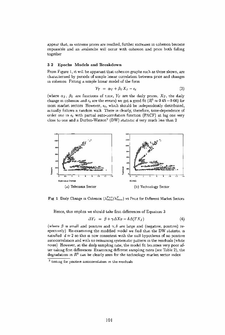
appear that, as extreme prices are reached, further increases in cohesion become impossible and an avalanche will occur with cohesion and price both falling together
3 2 E pochs M odels and B reakdow n
From Figure 1 , it will be apparant th a t cohesion graphs such as those shown, are characterised by periods of simple linear correlation between price and changes in cohesion Fitting a simple linear model of the form
Y t = OLT + f a X i + ¿ t ( 3 )
(where a j , fa are functions of time, Yt are the daily prices, X t , the daily change in cohesion and et are the errors) we get a good fit (R 2 « 0 45 — 0 6 6 ) for most m arket sectors However, et, which should be independently distributed, actually follows a random walk There is clearly, therefore, time-dependence of order one in et with partial auto-correlation function (PACF) at lag one very close to one and a Durbin-W atson2 (DW) statistic d very much less than 2
Eigenvalue Chang« ECttG
(a) Telecoms Sector (b) Technology Sector
Fig 1 Daily Change in Cohesion vs Price for Different Market Sectors
Hence, this implies we should take first differences of Equation 3
A Y f = £ + 7 A X T + 6 A ( T X r ) (4)
(where ¡3 is small and positive and 7 ,5 are large and (negative, positive) respectively) Re-examining the modified model we find th a t the DW statistic is satisfied d & 2 so this is now consistent with the null hypothesis of no positive autocorrelation and with no remaining systematic pattern in the residuals (white noise) However, a t the daily sampling rate, the model fit becomes very poor after taking first differences Examining different sampling rates (see Table 2), the degradation in R 2 can be clearly seen for the technology market sector index
2 testing for positive autocorrelation m the residuals
1 0 1

T able 2 Model Fit Statistics for Technology at Different Sampling Rates
Sampling Rate R2 Statistic DW Statistic
Monthly 0 46 1 97Every 10 Days 0 40 2 05Every 5 Days 0 40 2 20Every 2 Days 0 20 2 05
This d ata suggests th a t the variability (or volatility) increases markedly as the resolution increases and conversely th a t there is a settling period after which short term effects do not have an impact on subsequent data
3 3 Possible Reasons for Model Breakdown
As we have seen above, the simple linear regression models break down for fine granularity of sampling There are several possible reasons for this
- Day of the week It seems possible th a t market behaviour on certain days of the week, is subject to increased/reduced activity, reflecting start-up, closure and similarly We rejected this explanation, however, as eigenvalue changes and hence changes in cohesion were highly variable for all same-day data without exception
- Statistical leverage or outliers This presumes th a t extreme values occurring a t certain time points or reflecting abnormally large localised price fluctuations are peculiar to a high sampling rate This does not seem to be the case, since even very coarse-grained sampling, (i e monthly), retains the epoch skeleton Furthermore, while epoch turning points are clearly significant, the fit is satisfactory for lower sampling rates, but not for high ones Similarly, outlying points appear to have little influence on the R 2 or Durbin- Watson statistics for all rates and, in any case, are relatively few in number It does seem likely, however, th a t there exists a settling period m the market, a few days m length, during which high variability diminishes the fit
- Other systematic features Even at the daily rate, (fine-grained sampling), first-order filtering satisfactorily results in white noise Unfortunately, the relatively poor level of fit achieved for these higher sampling rates indicate th a t the model is significantly less reliable in terms of predictability value
W hat does seem clear is th a t the increased variability over a few days, reflects high volatility associated with changes m cohesive or co-operative behaviour, with frequent changes of the sign of the largest eigenvalue, (the linear trend is in any case strictly non-monotomc) It is, therefore, instructive to consider the nature of the volatility measure in more detail
Clearly, implied/price volatilities will change no matter what so th a t the historical basis should be relatively bias free Equally, A^oz is an effective measure of volatility, so th a t the change AC r+ i m the coherence is equivalent to looking at proportional change in volatility Typically, these high-frequency fluctuations
102

are self-correcting, representing d short-term and not particularly far-reaching lack of cohesive m arket behaviour, 1 e AC t +\ w 1 In other words, if coherence represents the change in commonly-perceived risk, deviation from the common perception is sufficient to ensure fluctuating variability over the short-term and corresponding reduction in fit, as observed for our data
While this position is usually resolved over a slightly longer period, it is the lack of a sustained common perception of risk, (1 e lack of coherence), which leads to a drop in price The quantity ACj +i is clearly large and negative at the turning point of an epoch, corresponding to large change m the maximum eigenvalue, as well as a change of sign, since no change of sign for A^aa. between consecutive time points implies th a t C is incremented Unfortunately, since high variability is naturally associated with short-term effects, as mentioned previously, it is non-tnvial to determine whether a sustained change can be determined in advance A number of points are worth noting, however Firstly, use of the covariance measure exposes the detail of these changes The epochs, while present to some extent in the correlation m atrix information, are far less distinct and thus less useful for our purposes, while dimensionality considerations do not arise for indices Secondly, we note th a t outliers are few, so th a t tolerances can more readily be established on the size of high-frequency fluctuations (It seems clear th a t the price change distributions involved do not scale simply, since volatility is dependent on the time interval as usual) It is suggested th a t coherence provides an intermediate measure which can be directly linked to critical market uncertainty
4 C onclusions
We dem onstrate the existence of epochs in EURO-STOXX market sector data, where the change m the largest eigenvalue of the covariance m atrix of daily prices, varies linearly with time The evidence supports an implicit relationship between instantaneous volatility and the change in the maximum eigenvalue, but volatility patterns are, typically, dependent on the time intervals observed At the end of an epoch, the relationship changes, with smaller eigenvalue changes leading to the same price change Epochs are present in all market sectors, but are most strongly defined in the less-defensive sectors, such as technology, telecoms The epoch end is followed by a return to low coherence in market trading, due to disparate perception of risk Co-operative behaviour (or strong coherence) in market trading suggests th a t up-turn patterns are more varied and hence less easy to predict, whereas down-turn patterns are well-defined, due to a common perception of risk change As a final note, it should be mentioned th a t we attem pted to replicate the results for exchange rate data but as data were limited, partial support only was obtained for results reported here
103

The authors would like to acknowledge Dublin City University and the Institute of Numerical Computation and Analysis (INCA) for financial support for travel and Dr Michael M ura for his invaluable contributions and insights
References
[Elton et al (2002)] Elton, E J , Gruber, M J , Brown, S , Goetzmann, W Modern Portfolio Theory and Investment Analysis John Wiley and Sons (2002)
[Litterman & Wmkelmann(1998)] Litterman, R , Winkelmann, K Estimating Covariance Matrices, m Goldman Sachs Risk Management Series, Goldman, Sachs &; Co (1998)
[Bouchaud h Potters(2000)] Bouchaud, I -P , Potters, M Theory of Financial Risks - From Statistical Phybics to Risk Management, Cambridge University Press (2000)
[Zumbach et al (1999)] Zumbach, G O , Dacorogna, M M , Olsen, J L , and Olsen, RB Introducing a Scale of Market Shocks, O &, A Research Group Preprint GOZ 1998-10-01, (1999)
5 A c k n o w led g em en ts
104

Noise in the correlation matrix: A simulation approach
Saba Sharifi Atid Shamaie Martin CraneSchool of Computer Applications
Dublin City University
The lesults ot apphing Random Matrix Theory (RMT) m finance suggest that the historical correlation matrix, , carnes a large amount ot noise The purpose of RM1 is to compart the statistical properties oi with those ol a random matrix By applying RM f we study how responds to the ditfeient volumes of noise in data
Wc generate a set of 4^0 random sinusoidal time series and add some random noise normally distributed with zero mean and a particular standard deviation The volume ot noise is controlled b> its standard deviation
Maximum 11 eigenvalue devnted1 from nndom bind
i . 3 i______ i______ i.______i____I________ ,____ I0 5 10_ 15 20 25 30 35Eigenvalues
500 1000Observations
The distributions of the eigenvalues m historical and random cases are plotted A large part of the histoncal graph is similar to the random one This part that is carrying noise corresponds to the noisy band of There are some eigenvalues that deviate trom the random graph These eigenvalues and the corresponding part ot have information and are known as the non-noisy band To estimate the exact effect of the added noise v\e increase the volume of noise gradually Starting from 0 02 11 diiierent values of standard deviation are examined and the number of deviated eigenvalues is estimated
1500
2 3Noise standard deviation
At the beginning by increasing the standard deviation an increase u\ the number ot deviated eigenvalues is observed But for the standard deviation varying from 0 08 to 4 no dramatic change is observed Therefore it indicates that fiom a particular point onward there is no relationship between the volume of noise and the number of non noisy eigenvalues or in the othei words, amount ot noise has no eftect on the number of noisy eigenvaluesConsequently we conclude that the volume of noise m the data has almost no effect on the genuine information part of the eigenvalues oi the correlation matrix This represents that except for very small volumes of noise involved in data RMT result is the same tor different amounts of noise In the case of stock markets we conclude that RMT result does not depend on the different volumes ol noise involved in stocks prices Whatever noisy the stocks pi ices are RMT estimates the same percentage oi the deviated eigenvalues ot trom the noisy bound
Contact ssabi@computing dcu ic 2jrd Conference on Applied Statistics in Ireland May 2003
105D C U