Navy Personnel Research and Development Center San Diego, California 92152-7250 TN-95-5 July 1995

Potential Utility Increases From Adding New Tests to the Armed Services Vocational

Aptitude Battery (ASVAB)

Frank L Schmidt Wendy L Dunn

The University of Iowa

John E. Hunter Michigan State University

19950810 001 sA

DTIl QUALITY INSPECTED 3

Approved for public release; distribution is unlimited.

NPRDC-TN-95-5 July 1995

Potential Utility Increases From Adding New Tests to the Armed Services Vocational Aptitude Battery (ASVAB)

Frank L. Schmidt Wendy L. Dunn

The University of Iowa

John E. Hunter Michigan State University

Reviewed by John H. Wolfe

Approved and released by Kathleen E. Moreno

Director, Personnel and Organizational Assessment

Approved for public release; distribution is unlimited.

The views, opinions, and/or findings contained in this report are those of the authors and should not be construed as an official Department of the Navy position, policy, or decision, unless so designated by other documentation.

Navy Personnel Research and Development Center San Diego, CA 92152-7250

REPORT DOCUMENTATION PAGE Form Approved OMB No. 0704-0188

Public reporting burden for this collection of information is estimated to average 1 hour per response, including the time for reviewing instructions, searching existing data sources, gathering and maintaining the data needed, and completing and reviewing the collection of information. Send comments regarding this burden estimate or any other aspect of this collection of information, including suggestions for reducing this burden, to Washington Headquarters Services, Directorate for Information Operations and Reports, 1215 Jefferson Davis Highway, Suite 1204, Arlington, VA 22202-4302, and to the Office of Management and Budget, Paperwork Reduction Project (0704-0188), Washington, DC 20503.

1. AGENCY USE ONLY (Leave blank) 2. REPORT DATE

July 1995 3. REPORT TYPE AND DATES COVERED

Final—September 1988-August 1989

4. TITLE AND SUBTITLE Potential Utility Increases From Adding New Tests to the Armed Services Vocational Aptitude Battery (ASVAB)

5. FUNDING NUMBERS Program Element: 0602233N

Work Unit: 0602233N.RM33M20.04 Contract Number DAAL03-86-D-001

6. AUTHOR(S) F. L. Schmidt, J. E. Hunter, W. L. Dunn

7. PERFORMING ORGANIZATION NAME

Battelle Memorial Institute 200 Park Drive, Suite 211 P.O. Box 12297, Research Traingle Park, NC 27709-2297

8. PERFORMING ORGANIZATION REPORT NUMBER TCN 86-698

9. SPONSORING/MONITORING AGENCY NAME(S) AND ADDRESS(ES) Navy Personnel Research and Development Center 53335 Ryne Road San Diego, CA 92152-7250

10. SPONSORING/MONITORING

NPRDC-TN-95-5

Functional Area: Product Line: Effort:

Personnel Systems Computerized Testing New Measures of Ability

12a. DISTRIBUTION/AVAILABILITY STATEMENT Approved for public release; distribution is unlimited.

12b. DISTRIBUTION CODE A

13. ABSTRACT (Maximum 200 words) This research examined whether the validity and classification utility of the Armed Services Vocational Aptitude Battery

(ASVAB) could be increased by adding additional predictors. The relevant literature indicated that ASVAB validity could be augmented by adding measures of (1) perceptual ability (to increase the validity of the ASVAB measurement of general mental ability) and (2) psychomotor ability. Adding perceptual ability increased the classification utility of the ASVAB by about 3%; the dollar value of this percentage increase increases over years of use of the augmented ASVAB, eventually building up to approximately $83 million per year. Adding both perceptual and psychomotor ability to ASVAB increased classification utility by approximately 5%. The eventual asymptotic value of this increase is $138 million per year. Augmenting the ASVAB produced unequal performance increases for more versus less complex jobs; this fact may be of importance to Navy policy formulation.

14. SUBJECT TERMS

Selection and classification, ASVAB, utility analysis, discretionary PCS moves, classifications, forecasting

15. NUMBER OF PAGES

46

16. PRICE CODE

17. SECURITY CLASSIFICA- TION OF REPORT

UNCLASSIFIED

18. SECURITY CLASSIFICA- TION OF THIS PAGE UNCLASSIFIED

19. SECURITY CLASSIFICA- TION OF ABSTRACT

UNCLASSIFIED

20. LIMITATION OF ABSTRACT

UNLIMITED

NSN 7540-01-280-5500 Standard Form 298 (Rev. 2-89) Prescribed by ANSI Std. Z39-18 298-102

Foreword

The purpose of this research was to establish the maximum potential gains in the utility of Navy personnel selection and classification that could result from adding additional ability tests to the current Armed Services Vocational Aptitude Battery (ASVAB). The work was funded by Program Element 0602233N, Work Unit 0602233N.RM33M20.04, sponsored by the Office of Chief of Naval Research (Code 01).

The authors would like to acknowledge the assistance of Drs. David L. Alderton and John J. Pass in obtaining the information on Navy enlisted jobs used in this research. The Center's technical monitor for this research was Dr. John J. Pass. This research was supported through the Scientific Services Program at Battelle Memorial Institute, Research Triangle Park, NC 27709 under contract DAAL03-86-D-001, Delivery Order 0053, TCN 86-698.

This report was received from the contractor in 1987. It is being published at this time because of its relation to later work. It was the precursor to more sophisticated cost-benefit analyses of adding new tests to the ASVAB, and it led directly to two projects to validate experimental computerized tests: the Navy Study of New Predictors, and the Enhanced Computer Administered Test (ECAT) project.

KATHLEEN E. MORENO Director, Personnel Department and Organizational Assessment

ÄGftsordflss For

MIC TAT> D

i JuDtifleal ion

* -II

Contents

Page Introduction l

Purpose 1

Estimation of Incremental Validities and Standardized Regression Equations 1

The Selection Utility Model Versus the Classification Utility Model 7 The Cohort Versus Equilibrium Models for Estimating Classification Utility 9 The Role of Promotion in Utility Estimation 10

Calculating the Figures Needed to Apply the Equilibrium Model 10 Rates and Ratings 12

Complexity Level 13

Navy Jobs with Cross-Matched Directory of Occupational Titles (DOT) Codes 13 Navy Jobs With no Cross-matched Directory of Occupational Titles (DOT) Codes 14 Determination of the Rejection Rate 15 Scaling of Relative Mean Output Levels 16

Scaling of the Standard Deviation of Individual Differences in Output 17 Determination of Final Regression Equations 17 Computing Classification Utility 18 Classification Methods 19

Current ASVAB 19 Augmented ASVAB—Cognitive Ability Alone 20 Cognitive and Psychomotor Ability 20

Results and Discussion 21

References 25

Appendix A—Description of Perceptual and Psychomotor Abilities A-O

Appendix B—Optimal Personnel Classification BO

Distribution List

vu

List of Tables

Page

1. Mean Validities for Three Ability Factors as a Function of Job Complexity for Performance on the Job (From Hunter, 1980a) 3

2. Beta Weights for GVN and KFM, Multiple Correlations, and Increments to the Validity of GVN Produced by KFM (From Hunter, 1980a) 3

3. Databases for Which complete Path Analyses Were Performed by Hunter (1983) 4

4. Increments to ASVAB Validity for Job Performance Based on Literature Review 6

5. Standard Score Regression Equations for ASVAB by Complexity Level 7

6. List of Ratings and Nonrated Occupations Used in Data Analysis 11

7. Distribution of Navy Enlisted Personnel by Job Complexity Levels (FY85) 15

8. Mean Enlisted Rates and Mean Compensation for Navy Enlisted Personnel by Job Complexity Level 16

9. Navy Enlisted Intake Figures for FY85 16

10. Final Regression Equations Used for Percentage Increase in Output Analysis 18

11. Final Regression Equations Used for Dollar Value Analyses 18

12. Optimal Classification of U.S. Navy Applicants Varying on Cognitive and Psychomotor Ability 21

13. Scaled Mean Job Performance Resultsa 21

14. Results in Percentages 22

15. Estimated Dollar Value of Absolute Output 23

16. Incremental Gains in Utility in Dollars 24

vm

Introduction

Purpose

The purpose of this research was to estimate the gains in the utility of Navy personnel selection and classification that could result from adding additional ability tests to the current Armed Services Vocational Aptitude Battery (ASVAB). This research focused on ability measures only (it did not include such potential predictors as biodata, measures of interests, personality, etc.).

Estimation of Incremental Validities and Standardized Regression Equations

One item of information critical to any estimates of utility gains is knowledge of the increments to validity that would be produced by the addition of ability tests. The final estimates of potential utility gains will depend directly on the estimated increases in validity expected to result from augmenting the ASVAB with new ability measures. Hence, the credibility of the final utility estimates (and of this research as a whole) depends on the credibility and accuracy of the estimates of incremental validity that are possible. This fact was a primary consideration determining the way in which the literature review providing the basis for the estimates of incremental validity was conducted. This document describes that process.

The research literature on human abilities consists mostly of small sample studies, including small sample validation studies. In the not too distant past, many researchers believed that such studies could individually yield useful and reliable information on many questions, including the questions of concern here: (1) what measures will produce increments to the validity of an existing battery and (2) how large will these increments be? For example, a study based on 300 to 400 cases reporting an incremental contribution to validity of .10 from the addition of a mechanical ability test to an existing test battery would often in the past have been interpreted as strong evidence for a real validity increment. And this was often true even when sample sizes were much smaller than 300 to 400 (e.g., 75 to 200). In recent years, however, the development and application of meta- analysis and validity generalization methods (Schmidt & Hunter, 1977,1981; Hunter, Schmidt, & Jackson, 1982; Callender & Osburn, 1980; Raju & Burke, 1983) has resulted in a better understanding of the instability and limited information of single studies. It is now clear that single studies cannot be interpreted in isolation, but must be combined with other studies in a meta- analysis to control for the effects of sampling error and other artifacts that distort obtained results (Hunter et al., 1982).

The cumulative findings of such "studies of studies" yield results and conclusions that are stable and replicable, despite the fact that the individual studies included in such quantitative reviews do not. This principle assumes even greater importance when the task is to estimate not validities per se, but increments to validities. Such increments are much smaller, have more sampling error (both absolutely and relative to their magnitudes), and are therefore more unstable from study to study. In light of these considerations, it would be inadvisable to focus the present literature review on individual studies. It is critical to the accuracy, and therefore the value, of this research that the estimates of incremental validity be as accurate as possible. It is particularly important to avoid the overestimates of incremental validities that would be likely to result from focusing on individual "successful" studies. This process of capitalizing on chance would lead to overstatements of utility gains from adding new tests to the existing ASVAB. This means, then,

that the literature review should focus on existing meta-analyses of large databases, because only such analyses can address questions of incremental validity at the level of precision required in this research.

Many meta-analyses have been conducted that (1) are based on large databases and (2) examine validities of a variety of abilities for performance on the job and in training. Schmidt and Hunter (1981) and Schmidt, Hunter, Pearlman, and Hirsh (1985) provide listings of such studies. For example, the meta-analysis by Pearlman, Schmidt, and Hunter (1980) was based on 3,368 validity coefficients and 10 different abilities. However, for our present purposes, most such available meta-analyses have two shortcomings. First, they are limited to one occupational area or job. For example, Pearlman et al. (1980) is limited to clerical work; Hirsh, Northrop, and Schmidt (1986) is limited to law enforcement occupations. Second, the validity coefficients for any given ability are based on a variety of different measures of that ability, instead of being from a single multi-aptitude test battery. Therefore, these studies do not as readily allow estimation of increments to validity from different abilities and ability composites. The data in these studies do allow estimates of incremental validity to be computed if one can obtain accurate estimates of test type (ability) intercorrelations. Such estimates can sometimes be obtained from test manuals and other sources, and such estimates are often used in estimating multivariate (that is, ability composite) validities for test batteries that are employed based on validity generalization findings. However, estimates of validity increments obtained in this manner are not likely to be as precise as those derived from meta-analyses of large databases in which all data are based on a single multi-aptitude test battery. In the latter case, all validities are for the specific measures in the test battery, and all intercorrelations among battery tests are known with high precision.

The first meta-analysis that meets the above criteria was conducted by Hunter (1980a) on the cumulative database of the General Aptitude Test Battery (GATB) (U.S. Department of Labor, 1970). This database consisted of 425 validity studies against criteria of performance on the job, and 90 studies based on criteria of training performance. Total sample size was approximately 23,100. In an earlier study (Hunter, 1980b), found that this widely used civilian battery tapped three general ability factors: (1) general cognitive ability (symbolized GVN), (2) perceptual ability (symbolized SPQ), and (3) psychomotor ability (symbolized KFM). (Descriptions of SPQ and KFM are given in Appendix A.) The database permitted accurate corrections for range restrictions and criterion unreliability. Using the "Data" and "Things" code from the Dictionary of Occupational Titles (U.S. Department of Labor, 1977), he classified each job into one of five "complexity" levels, where complexity was defined as the level of cognitive information processing demands imposed by the job. A critical finding was that the validities of GVN and KFM were complementary. As the complexity level of jobs increased, the validity of GVN increased. Conversely, as the complexity level of jobs decreased, the validity of KFM increased. As a result, the validity of a properly weighted composite of GVN and KFM was reasonably constant across complexity levels.

This project is primarily concerned with validities and incremental validities for performance on the job; it is these increments that have the major impact on utility gains. Table 1 summarizes the validity findings for the three ability factors by complexity level. The validity gradations described above for GVN and KFM can be plainly seen. It should be noted that complexity values for levels 1 and 2 are essentially identical; the ordering of complexity levels 1 and 2 is therefore arbitrary and can be reversed, which makes the validity gradations monotonically perfect for GVN and KFM. Hunter (1980a) found that, except for complexity level 1, SPQ made no incremental contribution to overall validity. Table 2 shows the beta weights and multiple correlations for GVN

and KFM by complexity level. This table also shows the increments to the validity of GVN produced by KFM at each complexity level. These are shown as numerical increments and in percentage terms. These findings indicate that KFM increments the validity of GVN at least slightly at all job complexity levels except one. The increment is extremely large at the lowest complexity level; however, as will be seen later, there are no Navy enlisted jobs at this level of complexity. These jobs are mostly feeding and off-bearing jobs; that is, feeding materials into machines and carrying off machine output on the other end.

Table 1

Mean Validities for Three Ability Factors as a Function of Job Complexity for Performance on the Job

■ (From Hunter, 1980a)

Mean True Validities Complexity Levels 1. Setup 2. Synthesize/coordinate 3. Analyze/compile/compute 4. Compare/copy 5. Feeding/off-bearing Note. GVN=general cognitive ability, SPQ=perceptual ability, KFM=psychomotor ability, 1 = highest level of complexity.

Table 2

Beta Weights for GVN and KFM, Multiple Correlations, and Increments to the Validity of GVN Produced by KFM

(From Hunter, 1980a)

GVN SPQ KFM .56 .52 .30 .58 .35 .21 .51 .40 .32 .40 .35 .43 .23 .24 .48

Beta Weights R Ar Complexity Level GVN KFM Percent Increase

1 .52 .12 .57 .01 1.8 2 .58 .01 .58 .00 0.0 3 .45 .16 .53 .02 3.9 4 .28 .33 .50 .10 25.0 5 .07 .46 .49 .26 113.0

NOTE. GVN = general cognitive ability, KFM = psychomotor ability, R = multiple correlation, Ar = increase in R.

In addition to the analysis of GATB data, a series of large sample meta-analyses of military data sets are also capable of yielding the level of precision in estimating incremental validities that is needed in the present research. Hunter (1983) reanalyzed the extensive military data sets described in Table 3. The major finding in all these analyses is the central role of GVN, a finding with important implications for this research. Using confirmatory factor analysis and path analysis, Hunter found that in all these data sets battery validity was entirely explained by GVN. Specifically, the validity of individual subtests in each battery is entirely accounted for by the aptitudes (that is, higher order factors that determine subtest scores). In turn, the validity of the aptitudes is entirely explained by GVN. These data showed that, within the cognitive domain, "there is, at most, very limited room for the presence of differential patterns of validity" (p. C-39).

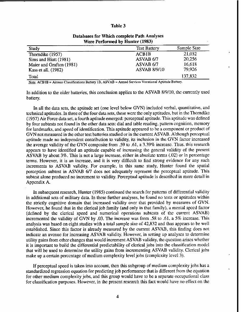
Table 3

Databases for Which complete Path Analyses Were Performed by Hunter (1983)

ACB1B 21,032 ASVAB 6/7 20,256 ASVAB 6/7 16,618 ASVAB 8/9/10 79,926

137,832

Study Test Battery Sample Size Thorndike (1957) Sims and Hiatt (1981) Maier and Grafton (1981) Kass et all. (1982)

Total Note. ACB1B = Airman Classifications Battery IB, ASVAB = Armed Services Vocational Aptitude Battery.

In addition to the older batteries, this conclusion applies to the ASVAB 8/9/10, the currently used battery.

In all the data sets, the aptitude set (one level below GVN) included verbal, quantitative, and technical aptitudes. In three of the four data sets, these were the only aptitudes, but in the Thorndike (1957) Air Force data set, a fourth aptitude emerged: perceptual aptitude. This aptitude was defined by four subtests not found in the other data sets: dial and table reading, pattern cognition, memory for landmarks, and speed of identification. This aptitude appeared to be a component or product of GVN not measured in the other test batteries studied or in the current ASVAB. Although perceptual aptitude made no independent contribution to validity, its inclusion in the GVN factor increased the average validity of the GVN composite from .59 to .61, a 3.39% increase. Thus, this research appears to have identified an aptitude capable of increasing the general validity of the present ASVAB by about 3%. This is not a large increase, either in absolute terms (.02) or in percentage terms. However, it is an increase, and it is very difficult to find strong evidence for any such increments to ASVAB validity. For example, in this same study, Hunter found the spatial perception subtest in ASVAB 6/7 does not adequately represent the perceptual aptitude. This subtest alone produced no increment to validity. Perceptual aptitude is described in more detail in Appendix A.

In subsequent research, Hunter (1985) continued the search for patterns of differential validity in additional sets of military data. In these further analyses, he found no tests or aptitudes within the strictly cognitive domain that increased validity over that provided by measures of GVN. However, he found that in the clerical job family (and only in that family), a mental speed factor (defined by the clerical speed and numerical operations subtests of the current ASVAB) incremented the validity of GVN by .03. The increase was from .58 to .61, a 5% increase. This analysis was based on eight studies with a total sample size of 42,832 and thus appears to be well established. Since this factor is already measured by the current ASVAB, this finding does not indicate an avenue for increasing ASVAB validity. However, in setting up analyses to determine utility gains from other changes that would increment ASVAB validity, the question arises whether it is important to build the differential predictability of clerical jobs into the classification model that will be used to determine the utility gains from incrementing ASVAB validity. Clerical jobs make up a certain percentage of medium complexity level jobs (complexity level 3).

If perceptual speed is taken into account, then this subgroup of medium complexity jobs has a standardized regression equation for predicting job performance that is different from the equation for other medium complexity jobs, and this group would have to be a separate occupational class for classification purposes. However, in the present research this fact would have no effect on the

final results. In this research, our focus is on the increment in utility over the utility of the current ASVAB that results from adding new tests to the ASVAB. Including perceptual speed as a separate predictor for clerical jobs would increase by a small amount the estimated utility of both the current ASVAB and the augmented versions of the ASVAB, but would leave the difference between these unaffected. Thus the incremental utility of augmenting the ASVAB would not change. In view of this, we did not develop a separate equation for clerical jobs. This procedure has one effect, however, that should be noted. In order to determine the utility gain from augmenting ASVAB, we must first estimate the gain over random assignment of applicants to jobs that could be produced by the current ASVAB if it were used optimally. Because of our procedure here, this latter estimate will be slightly lower than it otherwise would have been. However, the ASVAB is not currently used optimally now (see below), and our figure does not underestimate the current operational value of the ASVAB. In any event, estimation of the utility of the current ASVAB over random selection is not a primary purpose of this research.

A final large sample finding by Hunter (1984) is relevant to the present research. The findings reviewed up to this point indicate that, with the exception of clerical jobs, all of the validity of the ASVAB is due to its measurement of GVN. GVN is one of the two major predictive abilities measured by the GATB; the other, KFM, is outside the cognitive domain. How valid is the ASVAB measurement of GVN in comparison to the GATB measurement of the same ability? Hunter (1984) found that the ASVAB measure is more complete; it measures more of the aptitudes that are products of GVN. In particular, the ASVAB contains good measures of technical aptitudes, while the GATB does not. As a consequence, he found that although the GVN measured by the two batteries was the same factor, the validity of the ASVAB measure for predicting job performance was 9% larger. This finding will be useful in the present research since, as we will see later, it will be necessary to adjust GATB-based validities to obtain the comparable values for the ASVAB.

Our review focused only on large sample meta-analytic studies because only such studies are capable of providing the level of precision in estimating incremental validities that is needed in this research to ensure accuracy and credibility for the final utility gain figures. The research reviewed does not include every measurable ability, or even every measurable cognitive ability. Therefore, potential incremental validities from some abilities cannot be assessed. This fact is due to the nature of the research literature. In our judgment, the current literature is not capable of providing precise estimates of incremental validities for those abilities not included in the large scale studies reviewed above.

The findings reviewed above indicate that the cognitive domain validity in multi-test batteries stems from the battery's measurement of GVN. Therefore, it appears that all incremental validities should be estimated as increases in validity over and above that attainable from the measure of GVN contained in, and extractable from, the current ASVAB; that is, Forms 8/9/10 and equivalent forms such as ASVAB 14. There are two ways such increments could occur:

1. A new measure added to the ASVAB may contribute to improved measurement of GVN, thus increasing the validity of the measure of GVN obtainable from the battery. Our review indicates that an appropriate measure of perceptual aptitude should have this effect.

2. A new measure may assess an ability other than GVN which may increment the validity of an appropriately weighted sum. Our review indicates that KFM, if it could feasibly be added to the ASVAB, might function this way.

Table 4 presents the increments to ASVAB validity proposed for examination in this research. Column 1 indicates job complexity level as defined in Hunter (1980a). Column 2 presents our initial qualitative estimate of the frequency of Navy jobs in each complexity category; quantitative figures will later be inserted here. Column 3 lists the validities of the GATB measure of GVN for performance on the job at each complexity level, and the following column gives the comparable figures for the ASVAB 8/9/10 based on Hunter's (1984) finding that these figures are 9% higher. Column 5 presents the increment to the validity of GVN expected from adding appropriate measures of perceptual aptitude to the ASVAB. Based on Hunter's (1983) analysis of the Thorndike (1957) data, this increment is 3.39%. (All figures have been rounded to two decimal places.) Column 6 presents the validity of the ASVAB measure of GVN expected after this increment. In Column 7 the increments to validity expected from adding an appropriate measure of KFM to the ASVAB are listed. These values have been calculated using the validities in Column 6, the validities for KFM from Table 1, and the correlation between psychomotor and GVN from Hunter (1980a) (i.e., .35). The values in parenthesis are those originally reported by Hunter (1980a) for the GATB data; because the validity of the general ability measure in the augmented ASVAB is greater (compare Columns 6 and 3), these increments are no longer correct.

Table 4

Increments to ASVAB Validity for Job Performance Based on Literature Review

(1) (2) (3) (4) (5) (6) (7) (8) (9)

Complexity Enlisted Validity of Validity of Ar from New r of Ar from Final Total

Level MOS GATB ASVAB-Ga Perceptualb ASVAB-G Psychomotor0 *mult AR

1 Some .56 .61 .02 .63 .01 (.01) .64 .03

2 Few .58 .63 .02 .65 .00 (.00) .65 .02

3 Many .51 .56 .02 .58 .01 (.02) .59 .03

4 Many .40 .44 .02 .46 .08 (.10) .54 .10

5 Fewd .23 .25 .01 .26 .23 (.26) .49 .24

Note. ASVAB = Armed Services Vocational Aptitude Battery, MOS = military occupational specialty, GATB = General Aptitude Test Battery, ASVAB-G = general ability factor of the ASVAB. "Nine percent larger than GATB-G validities (see Hunter, 1984). bBased on Hunter's (1983) analysis of Thorndike (1957) data. 'Values in parentheses are from Hunter (1980a) for the GATB. Values outside parentheses were calculated for the ASVAB. dIt was later found that no Navy enlisted jobs fall into this complexity level.

Column 8 in Table 4 shows the final multiple correlation (overall validity) at each complexity level. These values were computed as described above. Finally, the last column shows the total increment to overall validity produced by adding both perceptual aptitude and KFM. With the exception of complexity levels 4 and 5, the absolute magnitude of these increments is modest. In percentage terms, the increments are 5, 3, 7, 27, and 112% for complexity levels 1 through 5, respectively. As noted earlier, there are no Navy jobs at complexity level 5. From the perspective of selection alone, increases in utility in the 3 to 7% range probably have substantial practical value. In addition, the differential predictability made possible by KFM may make possible further utility gains. Thus, even though our most accurate estimates of increments to validity are not large, the practical implications may still be substantial.

Table 5 shows the standardized regression equations derived from the figures in Table 4 (in concert with the correlation of .35 report by Hunter, 1980a, between psychomotor and GVN). In addition to the 5 complexity levels, equations are provided for complexity levels 1 and 2 combined.

These two levels, as noted earlier, do not actually differ in complexity, and were combined in the later utility analyses. The combined equations presented here take into account the relative numbers of Navy enlisted personnel at complexity levels 1 and 2; as described later, there are far more enlisted personnel at level 2 than at level 1. Equation sets 3,4, and 6, modified to reflect job family information on SD^ (the standard deviation of performance in dollars) and the mean value of job performance or output at different complexity levels, were used in the classification program to compute the estimates of utility gains from augmenting the ASVAB. Comparing Tables 2 and 5, it can be seen that increasing the validity of the measure of GVN has the effect of lowering the beta weights on KFM somewhat from the values obtained by Hunter in the GATB data. This is consistent with the decrease in the size of the validity increments as seen in Column 7 of Table 4.

Table 5

Standard Score Regression Equations for ASVAB by Complexity Level

Equation Set

Complexity Level Pre-Augmented

Augmented by Perceptual

Augmented by Perceptual and Psychomotor Multiple R

1 1 Zy = .61ZG Zy =.63Zo Zy= .60ZG +.09Zpm .64

2 2 Zy = .63ZG Zy =.65ZG Zy= .66ZG + .00Z/Jm .65

3 3 Zv = .56ZQ Z, =.58ZG Zv = .53ZG + XhZpm .59

4 4 Zy = .44ZG Zy =.46ZG Zy = .35ZG + .31Z/7OT .54

5 5 Zy = .25ZG Zy =.26ZG Zy= .12ZG +MZpm .49

6 l&2a Zy = .63ZG Zy = .65ZQ Zy= .66ZG +.005Z/7m .65

Note. ASVAB = Armed Services Vocational Aptitude Battery.

"In the classification analysis to follow, complexity levels 1 and 2 were combined to create the high complexity category. The standardized regression equations for this combined category are presented here. Because there are many more Navy enlisted personnel at complexity level 2 than 1, this group dominates the combined equations.

In summary, Tables 4 and 5 present the validity increments and associated standardized regression equations that in our judgment provide the most accurate and realistic basis for estimating utility gains from adding new tests to the current ASVAB.

The Selection Utility Model Versus the Classification Utility Model

The selection utility model has been discussed in detail by Brogden (1949), Cronbach and Gleser (1965), Schmidt, Hunter, McKenzie, and Muldrow (1979), and Hunter and Schmidt (1982b). This model is much simpler than is the case in classification. The selection model assumes available applicants will be evaluated for only a single job, whereas the classification model assumes each applicant will be assigned to one of several jobs. The task of the classification model is to assign individuals to jobs in such a way as to maximize overall productivity, while ensuring that each job receives the required number of workers. Classification always involves two or more real jobs. In addition, there may be a "reject" category; that is, the organization can reject at least some of the applicants rather than assigning them to one of the jobs.

Classification typically uses a separate equation for predicting success for each job or job family (Brogden, 1955,1964). The weight for a given test may differ from job to job, and may be zero for some jobs. The case in which one predictor is used for multiple jobs is called "placement."

In placement, if there is no reject category, the value of the slope of the regression line {rxyi SDy.) must differ from job to job in order for the gain in utility to be greater than zero (Cronbach & Gleser, 1965, chap. 5). The greater these differences, the greater the gain in utility. Even if the validity r™. is the same for all jobs, the utility of placement can still be substantial, if jobs differ significantly on SD... If there is a reject category, utility gains may stem primarily from rejection of poor prospects. In this case, the major determinant of utility gains is usually the size of r^ independent of differences between jobs in r^SD^..

The mathematical and measurement problems in classification are considerably more complex than in selection. However, Brogden (1946b, 1954) developed an iterative procedure that provides an optimal solution. For purposes of this research, we have developed a different solution, which is described later in the report text and in detail in Appendix B. In addition to estimates of SD,, for each job, the classification model also requires estimates of the average dollar value of the performance in each job. In selection, we need deal only with increments over this value and thus need not estimate absolute mean productivity (output) values for jobs. In terms of the economist, we need deal only with marginal utility in selection; in classification, we must deal with both marginal and absolute utility. This is one reason why the calculations for classification utility are more complex than for selection utility (Hunter & Schmidt, 1982b).

For any given job family or grouping we can write:

v= H + r^SDyZj + e

where

Zx is ability expressed in standard score units (mean 0, standard deviation 1),

v is individual performance on the job expressed in dollars,

|i is the mean performance in dollars of individuals selected to the job family without use of the test,

SDy is the performance standard deviation in dollars of persons selected to the job family without use of the test,

r„ is the population correlation between ability and performance (for the applicant population), and

e is the residual error of prediction. :

If a group of persons is_selected to a job family on the basis of ability,_and if the mean ability of that group is given by Zx, then the mean performance, ^_is given by y = (i + r^SDyZ^ This equation differs from selection equations for mean utility (U per selectee) in that it includes the term m. This equation gives the mean absolute level of productivity rather than the increment in productivity (i.e., marginal utility) resulting from use of the selection device. The term r^SDyZj is that increment (ignoring testing costs). This equation omits the term for testing costs, and will not, in general, consider testing costs in our analysis. This omission is justified by the fact that costs are negligible relative to utility gains. This is especially true in light of the need to prorate testing costs over the average tenure of the selectee. (Our utility estimates will be on a per year basis.) Mean performance on the job will be increased by use of the test to the extent that the numbers r^ SD^, and Zx are high (i.e., to the extent that job performance is highly related to ability, to the extent that there are great individual differences in performance, and to the extent that those selected have high mean ability).

For random selection, mean ability of those selected is the same as the mean for the applicant population as a whole, which is zero if ability is expressed in standard scores. Thus, for random selection, mean productivity for a given group is simply given by the constant [i for that group, which is the mean output for that job grouping. As described later, we estimate mean output as 1.75 times mean salary. The mean output for Navy enlisted personnel as a whole is the weighted average of these means, where each group is weighted by the number of persons in that group.

If job assignments are all made on the same ability (e.g., GVN), gains due to selection for one job family are partially offset by losses due to application of the same selection process to other jobs. Thus, if high-ability workers are assigned to one job, increasing productivity on that job, the remaining lower-ability workers must be assigned to other jobs, resulting in decreased productivity on those jobs. However, this cancellation effect will not be complete unless r^-SDy. is equal for all jobs. For this model, there is a maximum of counterbalancing between the gains produced by selecting the brightest for high complexity jobs, and the losses produced by selecting the dullest for low complexity jobs. However, because individual differences in output in dollars in high paying jobs (i.e., absolute values of SDy) are greater than such differences in lower paying jobs, the gains at the top will be larger than the losses at the bottom. Thus, there is a net gain from differential placement.

If different abilities are required in different jobs, then to the extent that those abilities are less than perfectly correlated, multivariate classification (i.e., classification on combined ability test scores) will be less prone to losses due to selection; that is, gains from selecting high-ability people for one job will be less offset by selection of low-ability people to other jobs than in the case of univariate selection (Brogden, 1959). Thus, there should be greater gains in overall utility for multivariate classification than for univariate classification.

The Cohort Versus Equilibrium Models for Estimating Classification Utility

There are two basic models that can be used in estimating the utility of both selection and classification. The best known and most commonly used is the cohort model. This model estimates utility based on the number of new employees hired per year—the annual cohort. To use this model, one must know or estimate the number assigned each year to each job family and the average time from assignment to termination for each job family. In the present research, it would also be necessary to know the complexity level of each job. This method yields the utility for each cohort over their tenure with the organization. That is, it yields the utility of 1 year's use of the test or battery. This utility results from use of the test or battery during that year, but is realized only over the period of time that the new employees remain with the organization.

The equilibrium model was used in Hunter and Schmidt (1982a) and is further discussed in Hunter, Schmidt, and Coggin (1987). This method estimates the utility an organization will realize per year once all incumbents in the job (selection) or set of jobs (classification) have been selected and/or assigned by means of the new procedure. This state is referred to as the equilibrium state. After an organization has attained equilibrium, the cohort and equilibrium models yield identical estimates of utility, as illustrated in Hunter et al. (1987). The Navy is an example of an organization in equilibrium: all or virtually all enlisted personnel have been selected and assigned using the ASVAB or an equivalent predecessor. Assuming for illustration that the longest tenure enlisted personnel have been in the Navy 20 years, the cohort model computes 1987 testing utility as the gain from using tests 20 years ago to select these personnel, plus the gain from using tests 19 years ago to select that cohort and so forth, all the way up to the gain from using the ASVAB in 1986 (to select the 1986 cohort). The sum of all these utility gains is the equilibrium gain in 1987.

The information needed to apply the cohort model could not be obtained from the Navy. Annual intake figures were available only by Navy rating. Each of the 102 Navy ratings covers a range of job complexity levels, and no information was available that would allow a breakdown of complexity levels within ratings for the annual intake cohorts. Also, estimates of mean time to termination for new recruits must be calculated from reenlistment rates, since no direct figures were available. However, reenlistment rates were not available by (and could not be computed for) complexity levels.

An advantage of the equilibrium model is that it does not require information on number hired per year or mean tenure with the organization. Instead, it requires the number and percentage of current incumbent personnel at each level of job complexity. (Because it is based on this "snapshot" of the organization, the equilibrium model is sometimes called the snapshot model.) For each complexity level, the model computes the value of mean performance when all incumbents have been selected and assigned using the procedure and the value when they were not so selected and assigned. The difference times the number at that complexity level is the utility gain at that complexity level. Total utility is the sum of these gains across all complexity levels. As described in the next section, we were able to obtain the necessary information from the Navy to apply the equilibrium model.

The Role of Promotion in Utility Estimation

It has long been clear that the cohort model produces large underestimates of utility in all cases in which substantial numbers of new hires are later promoted or advanced. The model assumes by default that people hired remain at the same level until they leave the organization. The further gains in utility resulting from promotion to jobs with larger SDy values (greater individual performance differences) are not captured. Unless special provision were made to modify it, the cohort model would assume that all Navy recruits remain at E-l, E-2, or E-3, until they leave the Navy. This is a gross distortion of normal progression for enlisted personnel.

The equilibrium model has a built-in allowance for promotion because it is based on the overall distribution of job complexity in the organization—not merely the job complexity distribution of new hires. In effect, it implicitly assumes that some individuals remain in low complexity jobs throughout and that some are in high complexity jobs from the time of hire—both of which are untrue or mostly untrue. However, these two assumptions counterbalance each other, providing a more accurate picture than the cohort model, especially in the case of an organization like the Navy in which there is substantial progression for most new recruits.

Calculating the Figures Needed to Apply the Equilibrium Model

To apply the equilibrium model, it is necessary to determine the number and percentage of Navy enlisted personnel at each complexity level. In this application, we also needed the mean salary at each complexity level (see below); this was easily calculated using the mean E-level at each complexity level, since current compensation levels for each of the nine E-levels were known. For each Navy rating (including unrated "ratings"), information was available showing the number of people in each rate or paygrade (E-l through E-9). Information was also available that allowed determination of the complexity level of each rate within each rating (e.g., E-6 of rating Aviation Boatswain's Mate E [ABE]). Table 6 shows the ratings and nonrated occupations used in the analysis. The procedures used to calculate the data needed to apply the equilibrium model are described in the next eight sections

10

Table 6

List of Ratings and Nonrated Occupations Used in Data Analysis

AB Aviation Boatswain's Mate ABE Aviation Boatswain's Mate—Equipment ABF Aviation Boatswain's Mate—Fuels ABH Aviation Boatswain's Mate—Handling AC Air Traffic Controller AD Aviation Machinist's Mate AE Aviation Electrician's Mate AF Aircraft Maintenanceman AG Aerographer's Mate AK Aviation Storekeeper AM Aviation Structural Mechanic AME Aviation Structural Mechanic—Safety

Equipment AMH Aviation Structural Mechanic—Hydraulics AMS Aviation Structural Mechanic—Structures AO Aviation Ordnanceman AQ Aviation Fire Control technician AS Aviation Support Equipment Technician ASE Aviation Support Equipment Technician—

Electrical ASM Aviation Support Equipment Technician—

Mechanical AT Aviation Electronics Technician AV Avionics Technician AW Aviation Antisubmarine Warfare Operator AX Aviation Antisubmarine Warfare Technician AZ Aviation Maintenance Administrationman BM Boatswain's Mate BT Boiler Technician BU Builder CE Construction Electrician CM Construction Mechanic CTA Cryptologic Technician—Administrative CTI Cryptologic Technician—Interpretative CTM Cryptologic Technician—Maintenance CTO Cryptologic Technician—Communication CTR Cryptologic Technician—Collections CTT Cryptologic Technician—Technical CU Construction Builder DK Disbursing Clerk DM Illustrator Draftsman DP Data Processing Technician DS Data Systems Technician DT Dental Assistant EA Engineering Aide

Ratings FTG GM GMG GMM GMT GSE GSM HM HT IC IM IS

JO LI LN MA ML MM

-Guns Fire Control Technician- Gunner's Mate Gunner's Mate—Guns Gunner's Mate—Missile Gunner's Mate—Technician Gas Turbine Technician—Electrical Gas Turbine Technician—Mechanical Hospital Corpsman Hull Maintenance Technician Interior Communications Electrician Instrumentman Intelligence Specialist

Journalist Lithographer Legalman Master-at-Arms Molder Machinist's Mate

MN Mineman

MR Machinery Repairman MS Mess Management Specialist MT Missile Technician MU Musician NC Navy Counselor OM Opticalman OS Operations Specialist OT Ocean Systems Technician OTA Ocean Systems Technician—Analyst OTM Ocean Systems Technician—Maintenance PC Postal Clerk PI Precision Instrumentman PM Patternmaker PR Aircrew Survival Equipmentman QM Quartermaster RM Radioman RP Religious Program Specialist SH Ship's Serviceman SK Storekeeper SM Signalman ST Sonar Technician STG Sonar Technician—Surface STS Sonar Technician—Submarine

11

Table 6 (continued)

Ratings EM Electrician's Mate SW Steelworker EN Engineman TD Tradevman EO Equipment Operator TM Torpedoman EQ Equipmentman UT Utilitiesman ET Electronics Technician WT Weapons's Technician EW Electronic Warfare Technician YN Yeoman FC Fire Controlman FT Fire Control Technician FTB Fire Control Technician—Ballistic Missile

Nonrated AA Airman Apprentice FA Fireman Apprentice AN Airman FN Fireman AR Airman Recruit FR Fireman Recruit CA Constructionman Apprentice HA Hospitalman Apprentice CN Constructionman HN Hospitalman CR Constructionman Recruit HR Hospitalman Recruit DA Dentalman Apprentice SA Seaman Apprentice DN Dentalman SN Seaman DR Dentalman Recruit SR Seaman Recruit

Rates and Ratings

The 20 September 1986, Annual Report: Navy Military Personnel Statistics provided the basic data. For each of the 102 ratings listed in the Annual Report, data are provided that list the number of Navy enlisted personnel on active duty as of 30 September 1986 within each of the rates (E-levels) in that rating. These data are published by rate title, which corresponds directly to E-level (paygrade) as follows:

E-4—Petty Officer Third Class (3) E-5—Petty Officer Second Class (2) E-6—Petty Officer First Class (1) E-7—Chief Petty Officer (C) E-8—Senior Chief Petty Officer (SC) E-9—Master Chief Petty Officer (MC)

In addition to personnel assignments within ratings, the Annual Report lists the number of personnel in each of the three nonrated paygrades (E-l through E-3) for each of the six apprenticeship occupational groups (seaman, hospitalman, dentalman, fireman, constructionman, and airman). These statistics on the nonrated personnel are further divided into those personnel who have been assigned a particular rating (called "strikers") and those who remain in the unassigned group.

12

In summary, data were available that allowed us to determine how many people were presently working in each paygrade for each Navy occupation.

Complexity Level

In Hunter's (1980a) work, complexity level was determined from the "data-people-things" dimension of the Directory of Occupational Titles (DOT) code assigned to each job in the U.S. Employment Service database. Many of the jobs in the Navy closely correspond to civilian jobs, and the DOT codes, which represent these comparable civilian jobs, are published in a document entitled Navy Enlisted Occupational Code Index. Other jobs are unique to the Navy (i.e., they have no civilian equivalent; therefore, they have no cross-matched DOT codes).

Navy Jobs with Cross-Matched Directory of Occupational Titles (DOT) Codes

The Navy Enlisted Occupational Code Index (pp. 91-119) lists the 102 naval ratings and cross- matches these ratings to DOT-coded civilian jobs that are comparable. Because job complexity changes as one progresses through the rates within each rating (from E-l to E-9), the ratings are broken into subdivisions corresponding to categories of different job tasks. For example, for the rating ABE, there are three general job categories: (1) one corresponding to E-levels 1 and 2, (2) one to E-levels 3 to 6, and (3) one to E-level 7. In addition, when a person advances past E-level 7 of rating ABE, he or she enters a different rating, AB, which includes E-levels 8 and 9. Some of these categories are cross-matched to civilian jobs and some have no civilian job equivalents.

For those categories with DOT cross-matches, the complexity level was determined according to Hunter's scheme. The fourth, fifth, and sixth digits of the nine-digit DOT code correspond to that job's requirements on the dimensions of Data, People, and Things, respectively. Hunter found that job complexity can be coded according to the following scheme:

1. If the Things code = 0, the complexity level is 1. 2. If the Things code = 6, the complexity level is 5. 3. If the Things code ^ 0 or 6, the complexity level is:

a. 2 if the Data code is 0 or 1. b. 3 if the Data code is 2, 3, or 4. c. 4 if the Data code is 5 or 6.

Complexity levels were calculated for all civilian jobs that were cited in the Index. In some cases, only one civilian job was listed as corresponding to a naval rating category. For example, on page 91, ABE 3 to 6 is cross-matched to the civilian job titled Aircraft Launch and Recovery Technician, which has the DOT code of 912-682-010. According to Hunter's coding scheme, this job is assigned a complexity level of 4.

In other cases, more than one civilian job was cross-matched to a naval rating category. In these cases, complexity levels were assigned to each of the civilian jobs, and the average of these complexity levels was the complexity level assigned to the naval ratings category. When the average was not a whole number, the average was rounded to the nearest whole number and that number was assigned as the complexity level for naval rating category. For example, if three civilian jobs were at complexity level 3 and one at level 4, the average of 3.25 was rounded to 3; if two jobs were at level 3 and two at level 4, the average of 3.5 was rounded to 4.

13

The complexity level assigned to each rating category was applied to all E-levels contained in that category. For example, the naval rating category of ABE 3 to 6 was of complexity level 4. This means that within the rating ABE, E-levels of 3,4, 5, and 6 were assigned a job complexity level of 4.

Navy Jobs With no Cross-matched Directory of Occupational Titles (DOT) Codes

Not all naval rating categories were cross-matched to civilian jobs with their accompanying DOT codes. Consequently, these rating categories were assigned complexity levels according to an evaluation of tasks they included. The tasks that were evaluated were found in the Manual of Navy Enlisted Personnel Classifications and Occupational Standards: Section I. Complexity levels were determined by choosing the best fit between the tasks and responsibilities required by each rating category and the following general descriptions of the jobs by each complexity level:

Complexity Level 1: These jobs represent the most complex technical jobs. They are jobs that require specialized and advanced training, and exclude jobs that are essentially managerial in nature. They are infrequent in this data set, but include jobs such as Boiler Technician E-8 and E-9 (civilian equivalent = engineer) and Lithographer E-7 through E-9 (with several civilian equivalents).

Complexity Level 2: These jobs are primarily managerial in nature. They include substantial components of management of other personnel, coordination of information from many different sources, decision-making, and evaluation. Many of the ratings include categories of these jobs at the highest E-levels. Examples include Air Traffic Controller E-7 through E-9 and Aviation Machinist's Mate, E-6 through E-8.

Complexity Level 3: These jobs are skilled jobs that require specialized training, and which typically are technical in nature. Many naval rating categories fit into complexity level 3, particularly at the E-levels of 3 through 6 or 7.

Complexity Level 4: These are the semi-skilled jobs that require some specific skills. They differ from level 3 jobs in that the skills required are less complex and can usually be learned in on-the-job training. They are less technical in nature. All jobs at E-l and E-2 were assigned this complexity level.

Complexity Level 5: These jobs are unskilled jobs that require very little or no training. Feeding and off-bearing jobs would be at this complexity level. However, the Navy has few, if any, jobs at this complexity level, and the data set used in this study did not include any rating categories that were coded at complexity level 5.

Complexity levels were determined by examining the tasks included in all of the E-levels subsumed by a rating category. For example, the complexity level for AB E-8 and E-9 was determined by inspecting the task requirements for both E-levels 8 and 9, and the single complexity level which was determined to best correspond with those tasks was assigned to both E-levels. This procedure is analogous to that used in assigning complexity levels to rating categories when civilian job equivalents were cross-matched.

In summary, complexity levels were determined for each rate within each rating listed in the Annual Report. In addition, complexity levels were assigned to all nonrated personnel categories for E-levels 1, 2, and 3.

14

Part I of Table 7 shows the number and percentages of Navy enlisted personnel at each of the five job complexity levels. There are no personnel at the lowest complexity level (level 5), and less than 1% at the highest complexity level (level 1). Part II of Table 7 shows the number and percentage at the three complexity levels used in all subsequent analyses. This complexity scheme differs only in that complexity levels 1 and 2 have been combined to form the high complexity category. The information provided by the Navy for this analysis yielded a total figure of 452,597 enlisted personnel. According to 8,609 Navy Jumps Submission, there are 507,820 enlisted personnel (FY86). Thus, 10.8% of Navy enlisted personnel appear to be "missing." The reasons for this discrepancy could not be immediately explained by Navy Personnel Research and Development Center (NAVPERSRANDCEN) personnel. The larger figure may include all individuals who were on duty for any part of FY86, while the smaller figure may include only those on duty during one time period during the year. Also, the smaller figure may exclude those on sick leave, those assigned to special projects, and those assigned to other government agencies. In any event, the figures used in subsequent analyses are those shown in Table 7. If they are about 11% low, the effect will be to reduce the obtained dollar utility estimates.

Table 7

Distribution of Navy Enlisted Personnel by Job Complexity Levels (FY85)

Complexity Level Number Percent I. Original Complexity Levels

1 (Highest) 3,465 .76 2 60,724 13.42 3 314,593 69.51 4 73,815 16.31 5 (Lowest) 0 .00

Totals 452,597 100.00 II. Modified Complexity Levels Used in the Analysis High(l&2) 64,189 14.19 Medium (3) 314,593 69.51 Low (4) 73,815 . 16.31

Totals 452,597 100.00

Table 8 shows the mean E-levels and mean salary levels for the original (Part I) and modified (Part II) job complexity categories. The uses made in this research of the mean salary figures are described in later sections of this report.

Determination of the Rejection Rate

As noted in a previous section, determination of classification utility requires that the percentage of applicants rejected because of low aptitude test scores be known. Table 9 shows data from FY85 relevant to this determination. Of the 140,083 applicants, 14,776 were rejected on the basis of their Armed Forces Qualification Test (AFQT) scores, yielding a rejection rate of 10.55%. Since, for purposes of this study, a round percentage was required, we conservatively rounded this figure down to 10%, rather than up to 11%. This will cause a slight underestimation of overall ASYAB utility (combined selection and classification utility), but will have no effect on the incremental utilities to be estimated.

15

Table 8

Mean Enlisted Rates and Mean Compensation for Navy Enlisted Personnel by Job Complexity Level

Complexity Level Mean E-Level Mean Salary

I. Original Complexity Levels 1 2 3 4

6.33 7.57 4.52 1.91

$32,772 33,090 23,018 9,570

II. Modified Complexity Levels Used in the Analysis

High (1 & 2) Medium (3) Low (4)

7.50 4.52 1.91

$33,073 23,018 9,570

Categoryd

Table 9

Navy Enlisted Intake Figures for FY85

1. Applicants 2. Recruits 3. Rejected—Low aptitudeb

4. Rejected—Medical 5. Rejected—Other

Number

140,083 87,660 14,776 6,443 1,075

al - (2 + 3 + 4 +) = 30,125. these applicants were not (permanently) rejected. This number includes individuals who decided not to enter military service, decided to enter a different service, or were temporarily rejected for a transient medical condition. It also includes a small number of people who took a different version of the AS VAB. bPercent rejected for low aptitude = 14,776 / 140,083 = 10.55%.

Scaling of Relative Mean Output Levels

As noted in a previous section, determination of classification utility requires an index of average value of output at each complexity level. The original plan in this research called for NAVPERSRANDCEN personnel to have Navy experts scale mean output value on a ratio scale using psychophysical methods (Guilford, 1954). When we learned this task could not be completed for this research, we developed an alternate method of scaling. The salary levels of different Navy enlisted rates (E-l through E-9) can be taken as proportional to the value that the Navy places on mean output or performance in the various rates. Once average salary at each complexity level is known, average overall salary can be used to scale the relative value of mean output at the different complexity levels. In our analysis, the mean was scaled to 100 for the total group, including rejects, whose scaled scores were all set to zero. The salary levels shown in Part II of Table 8 were used in this scaling. Further detail is provided in Appendix B.

This scaling yields the relative or proportional value of mean output at the three job complexity levels and is used in calculating percentage increases in output due to classification. To determine the dollar value of these increases, we must have estimates of the dollar value of mean output. In the economy as a whole, wages and salaries average 57% of the dollar value of output (Hunter & Schmidt, 1982a). This means that, on the average, the dollar value of mean output is 1.75 times

16

wages and salaries. This figure was used in this research. That is, for each complexity level, the dollar value of average output was estimated as 1.75 times the mean salary at that complexity level.

Scaling of the Standard Deviation of Individual Differences in Output

If mean output is known, and if the standard deviation as a percent of mean output (SD^) is known, then the standard deviation of output is simply the product of these two figures. For example, if mean output in dollars is $50,000 per year and if SDp is .25, then SD^ (the standard deviation of output in dollars) is (.25) ($50,000) = $12,500. SD^ values can be calculated only in data sets in which the output of individuals has been measured on a ratio scale (e.g., counts of number of products made). Such data sets are difficult to obtain and are therefore relatively infrequent. This means it is very important to locate and use all available cumulative data to obtain generalizable estimates of SDp that can be used with jobs for which it is not possible to compute SDp. The first such review and analysis was published by Schmidt and Hunter (1983) (see also Burke & Frederick, 1984). The data they were able to locate were mostly from semi-skilled (and some skilled) blue-collar jobs and from routine clerical jobs. For these jobs, they found that SD^ averaged 20% of mean output for non-piecework pay systems (15% for piecework systems).

This figure was for incumbents; it was not corrected to the applicant SD^ value, which would be the appropriate value and which would be larger. Since that study was completed, more data have become available. Since some of the new data are from medium and high complexity jobs, it is possible to compute SD„ values for each of the three complexity levels used in this study. This has been done by Hunter and Schmidt (1987), and the resulting figures have been adjusted for range restriction, so they apply to applicant populations rather than to incumbents. The average SDp values for high, medium, and low complexity were found to be .61, .36, and .25. These figures were used in the present study. In computing the standard deviation for the utility analysis in percentage increase terms, the standard deviation at each complexity level was its SD^, value times its scale score. In the dollar value analysis, SDy at each complexity level was its SD^ value times 1.75 (mean salary); that is, SDp times the value of mean output. The SD^ values for the three complexity levels were:

High: $35,305 Medium: 14,501 Low: 4,187

Determination of Final Regression Equations

Table 5 presented the regression equations in standard score form. But since the three complexity levels differ in both mean output value and standard deviation of output, standard score regression equations cannot be used in the classification program to conduct the utility analysis. Instead, the equations must be modified to reflect these differences among complexity levels. Table 10 shows these final regression equations for utility analysis of percent increase in output. Table 11 shows the corresponding equations for the dollar utility analysis. In these equations, ability remains in z-score form, but output is scaled either using our ratio scale (Table 10) or in dollars (Table 11). The dollar based equations in Table 11 were actually not explicitly used in the program, because the dollar value results were easily calculated from the percentage increase results. Nevertheless, they are the equations that were implicitly used (see Appendix B).

17

Table 10

Final Regression Equations Used for Percentage Increase in Output Analysis

Complexity Level Pre-Augmented

Augmented by Perceptual

Augmented by Perceptual and Psychomotor

High $ = 63.41ZG+165 y = 65.222^+165 $=66.35ZG-2.01^,m+165 Medium y = 23.18ZG+115 $ = 24,012^+115 $=21.87ZG+5.47Z/,m+ 115 Low Rejects

y = 5.28ZG +48 V = 0

y = 5.52ZG +48

$ = 0 y = 4.23ZG + 3.682^m + 48 $=0

Table 11

Final Regression Equations Used for Dollar Value Analyses

Complexity Level Pre-Augmented

Augmented by Perceptual

Augmented by Perceptual and Psychomotor

High

Medium

Low

Rejects

A y A y A y A y

22,242ZG+33,090 y

8,120ZG +23,018 y

1,842ZG + 9,570 y

0 y

22,948ZB + 33,090 y= 23,195ZG - 7042^,OT + 57,878

8,410ZG +23,018 y= 7,734ZG + l,933Zpm + 40,281

1,926ZG +9,570 y= 1,477ZG + l,284Z/)m + 16,747

0 y= 0

Computing Classification Utility

The basic analysis plan in this research calls for comparing the classification utility of the current ASVAB with the classification utility of (1) ASVAB augmented by SPQ and (2) ASVAB augmented by both SPQ and KFM. This means that the first step must be estimation of the utility of the current ASVAB. Obviously, the utility of the current ASVAB depends on how it is used. For numerous practical reasons, none of the services currently uses ASVAB in a manner that maximizes its potential classification utility (Foley, 1985; Kroeker & Rafacz, 1983; Maier & Fuchs, 1973). With the advent of the all volunteer services, it has become necessary to assign recruits to jobs individually or in small groups, instead of assigning large intake batch groups simultaneously.

This results in individual job assignments that would not be made if large groups were assigned simultaneously, and leads to reduced classification utility. Other variables currently built into the assignment decisions that are unrelated to utility are transportation costs to class "A" technical schools and minority fill rates. In addition, the utility of the current system is reduced somewhat because assignment is based on job family composites instead of the best possible measure of GVN (Hunter, 1983, 1985), and because the job families are not based on the complexity levels of jobs. Classification and Assignment Within PRIDE (CLASP)systems used in the Navy are described by Foley (1985) as follows:

18

Project Compass, a computer-assisted classification system for Navy enlisted men, is a batch- processing procedure based on the Ford-Fulkerson transportation algorithm. Its development and operation have been documented in Swanson and Dow (1965) and Hatch (1968). In brief, it fills school quotas by an overall best combination of men—the system maximizes the sum of selection test scores for the individual schools. This criterion, maximal test scores, is the same as used earlier with the hand assignment method. Later refinements included a component that maximized transportation costs (from site of Basic Training to Assigned "A" school), and a minority-fill quota to ensure representation across ratings. Compass was designed to optimally assign personnel when the assignees were aggregated, as at recruit training centers. With introduction of the all-volunteer force, it became necessary to accommodate individual preferences in order to be competitive with the enlistment practices of the other services. This new environment dictated development of an optimal sequential assignment system, such as embodied in CLASP, (p. 11)

The current system (the CLASP system) is now so complex (cf. Kroeker & Rafacz, 1983) that it would be difficult or impossible to determine what percentage of maximum potential utility of the current ASYAB is being attained. Thus, it is not feasible to work within the context of the current system in estimating the potential gains from adding tests to the ASVAB. Therefore, we decided to estimate the utility the ASVAB would have over random assignment if the ASVAB were used optimally in classification. This analysis yields the maximum potential utility of the ASVAB. The incremental utilities of SPQ and perceptual plus KFM were evaluated in the same way: as the maximum improvement they could make over the potential utility of the ASVAB.

Ignoring the differential predictability of clerical jobs (discussed earlier) using the perceptual speed measures in the current ASVAB, the classification utility of the current ASVAB is maximized by assigning recruits to jobs based on (1) GVN (as estimated by ASVAB subtests, AR, MK, WK, GS, El, and MC) (Hunter, 1983) and (2) job complexity levels. A computer program was written that estimates this utility. This program also estimates the utility yielded by the augmented regression equations shown in Tables 10 and 11. The differences are the incremental utilities from augmenting the ASVAB.

Classification Methods

The classification problem is solved for each of three cases: (1) optimum classification using only cognitive ability as measured by the current ASVAB, (2) optimum classification for the ASVAB augmented by SPQ, and (3) optimum classification based on the augmented measure of GVN used in combination with general KFM. The first two cases are single predictor cases that are easily solved using the methods of Hunter and Schmidt (1982). The third case is a two predictor case for continuous distributions. This case requires an extension of Brogden's (1955) methods.

Current ASVAB

The current ASVAB has no measure of KFM. Thus, optimal classification would be based on GVN alone. As shown in Appendix B, the optimal classification is obtained by placing the top 13% of applicants in high complexity jobs, placing the next 62% in medium complexity jobs, placing the next 15% in low complexity jobs, and rejecting the bottom 10%.

19

Augmented ASVAB—Cognitive Ability Alone

As shown in Appendix B, the augmented cognitive measure would be used in the same way as the unaugmented measure. Optimal classification is obtained by placing the top 13% of applicants in high complexity jobs, placing the next 62% in medium complexity jobs, placing the next 15% in low complexity jobs, and rejecting the bottom 10%.

Cognitive and Psychomotor Ability

Optimal classification using two predictors requires the solution of the classification problem for two continuously distributed predictors. The technical details of this process are given in Appendix B.

The method used here is to construct a set of 100 prototype individuals representing the joint distribution of applicants on the two predictors: GVN and KFM. Each prototype individual represents 1% of the distribution. For each decile of cognitive ability, there are 10 prototype individuals who differ on KFM. Because KFM is correlated .35 with cognitive ability (Hunter, 1980b), the 10 individuals within each decile of cognitive ability were not constructed using invariant levels of KFM. Rather, the levels of KFM were chosen differently within each level of cognitive ability so that the frequency represented by each prototype individual would be 1%. To do this, the 10 prototype individuals within each cognitive ability group were constructed so that they represent the deciles of KFM as a residual from the regression of KFM onto cognitive ability. That is, the 10 prototype individuals for one level of cognitive ability do not represent the same amounts of KFM as the 10 prototype individuals for another level of cognitive ability. Instead, the 10 individuals within each decile on cognitive ability vary about their own mean level of KFM rather than about the mean for the whole applicant population.

The optimal classification of applicants is shown in Table 12. The Navy applicant quota for high complexity jobs is 13% (Table 13). Table 12 shows that all 10 of the prototype individuals in the highest decile of cognitive ability are assigned to high complexity jobs. Among the 10 individuals in the second decile of cognitive ability, the seven with highest KFM are assigned to medium complexity jobs, while those with lowest KFM are assigned to high complexity jobs. Since medium complexity work depends on KFM while high complexity work does not, there would be greater loss of productivity if the high KFM individuals within this decile were assigned to high complexity work.

The Navy applicant quota for medium complexity work is 62% (Table 13). Of the 10 prototype individuals in cognitive decile 2, seven were assigned to medium complexity work. All the 50 individuals in cognitive deciles 3-7 were assigned to medium complexity work. In decile 8, the five individuals with high KFM were assigned to medium complexity work, while those with lower levels of KFM were either assigned to low complexity work or were rejected from service. This may appear to be paradoxical in light of the fact that the correlation between KFM and performance ratings is higher for low complexity work than for medium complexity work. The explanation lies in the consideration of raw score regression weights for the two levels of work. Because individual differences in productivity are much greater for medium complexity work than for low complexity work, the raw score regression weight of KFM is greater for medium complexity work than for low complexity work (see Table 10). That is, the net impact of KFM differences is greater for medium complexity work than for low complexity work.

20

Table 12

Optimal Classification of U.S. Navy Applicants Varying on Cognitive and Psychomotor Ability

High Relative Psychomotor Ability Decile Low

Cognitive Ability Decile 1 2 3 4 5 6 7 8 9 10

Highest decile 1 a a a a a a a a a a 2 b b b b b b b a a a 3 b b b b b b b b b b 4 b b b b b b b b b b 5 b b b b b b b b b b 6 b b b b b b b b b b 7 b b b b b b b b b b 8 b b b b b c c c c d 9 c c c c c c c c d d

Lowest decile 10 c c c d d d d d d d Not?. Classification groups are: a = high complexity jobs, b = medium complexity jobs, c = = low complexity jobs, d = rejected.

Table 13

Scaled Mean Job Performance Results3

Random Current Augmented by Complexity Levels Percent Assignment ASVAB-G Perceptual

Augmented by Perceptual & Psychomotor

High 13 165 268.34 271.60 270.56 Medium 62 115 118.94 119.08 119.74 Low 15 48 42.96 42.76 42.96 Rejects 10 00 00 00 00 Total-all 100 100 115.071 115.553 115.854 Total-accepted 90 111.11 127.857 128.392 128.727 aSDy7 values for High, Medium, and Low complexity levels are .61, .36, and .25, respectively. Mean output at the three complexity levels is assumed to be proportional to mean salary at those levels. Overall, mean salary ($20,006) is used to scale mean output for the total group (including rejects to 100). This scaling reflects the Navy's scaling of mean job value in terms of salary.

The Navy quota for low complexity work is 15% (Table 13) and the rejection rate is 10%. All those assigned low complexity work or rejected are in the bottom 3 deciles on cognitive ability. Within each decile, those higher on KFM are assigned to low complexity work while those lower are rejected. The proportion of those rejected is 10% in decile 8, 20% in decile 9, and 70% in decile 10.

Results and Discussion

Table 13 shows the results in terms of the scaled job values. The first column of numbers shows the percentage of applicants that will wind up in the four categories: high, medium, and low complexity jobs and the reject category. Since 10% are rejected, all the other percentages are less than those for incumbents given in Table 7. The "average value of job performance" of rejects is

21

scaled to zero, and the resulting mean scale value for all acceptees is 111.111. Under random assignment, the scaled value of mean performances is 165 and 115 in high and medium complexity jobs, respectively. Thus, the ratio of mean values is 165/115 = 1.43; that is, mean job performance in high complexity jobs is 43% more valuable than in medium complexity jobs. The same comparisons can be made for other complexity levels.

As expected, the largest increase in utility occurs in going from random assignment to optimal use of the current ASVAB. The further increases from augmenting the current ASVAB are much smaller, again as expected. Optimal use of the current ASVAB produces the largest gain at the high complexity level and a smaller gain at the medium complexity level. At the low complexity level, the gain is negative; this also is expected and is due to the trade-offs discussed earlier. Higher ability people are assigned to high complexity jobs, greatly increasing output and performance in those jobs; but this leaves fewer high ability people in the low complexity jobs, resulting in a (much smaller) reduction in output and performance there.

Table 14 shows these results in percentage terms. The first column shows the percent increase in output over random selection produced by optimal use of the current ASVAB. At the highest complexity level, this gain is almost 63%. At the lowest complexity level there is a loss of 10.5% and at the medium complexity level, a modest gain of 3.43%. The overall increase is 15.07%, a very substantial increase when evaluated in dollar terms, as we will see later. The second and third columns in Table 13 are computed on a different base: they are percent increases in the ASVAB gains shown in Column 1. That is, they reflect gains in the initial ASVAB gain, resulting solely from augmenting the ASVAB. As such, they are the figures of primary interest in this research. Adding SPQ to the current ASVAB produces an overall increase of 3.19% in ASVAB classification utility. Adding both perceptual and psychomotor yields an overall increase in utility of 5.20%. These gains in utility are not spread evenly over complexity levels. When the ASVAB is augmented by SPQ only, the effect is to produce a more valid measure of general ability. This intensifies the trade-off (which already exists with the current ASVAB) between increases in performance at higher complexity levels and decreases at the lowest complexity level. Thus, compared to the current ASVAB, there are utility increases at the high (3.16%) and medium (3.55%) complexity levels, but a further output decrease (- 3.97%) at the lowest complexity level. Because the majority of incumbents are in the high and medium complexity jobs (83.69%), the overall increase is positive (3.19%).

Table 14

Results in Percentages

Percent Increase in ASVAB-G Gain From:

Complexity Levels

"High Medium Low All

Percent Gain Over Random for ASVAB-G

Percent Gain Augmenting With

Perceptual

Augmenting With Perceptual and Psychomotor

62.63 3.43

-10.50 15.07

3.16 3.55

-3.97 3.19

2.15 20.30 0 5.20

Note. ASVAB-G = General ability factor of the ASVAB.

22

When the ASVAB is further augmented by KFM, this adds a new ability and therefore acts to reduce the intensity of the trade-off. There is no decrease in performance at the low complexity level; it remains the same as with the current ASVAB. There is a large increase (20.30%) in utility at the medium complexity level. The increase in utility at the high complexity level (2.15%) is less than results from augmenting ASVAB by SPQ alone (3.16%). This is because some of the people who are high in both GVN and KFM are now assigned to medium complexity jobs. When cognitive ability alone is used in classification, these people are assigned to the high complexity jobs.

In summary, the best estimate of the overall attainable increase in classification utility from augmenting the current ASVAB is 5.20%. It is not clear from this figure alone whether this increase is large or small in absolute terms. To judge this, we must turn to the results of the dollar utility analyses.

Table 15 shows the estimated dollar value of yearly output on performance at each complexity level for the four different job assignment strategies. These figures represent an intermediate step in this research and are not the primary focus. However, it is interesting to note that this model, based on generalizations from the civilian economy, estimates the yearly value of Navy enlisted personnel output at between $17.6 billion (random assignment) and $20.4 billion (fully augmented ASVAB).

Table 15

Estimated Dollar Value of Absolute Output

Complexity Levels Number

Random Assignment

Current ASVAB-G

Augmented by Perceptual

Augmented by Perceptual & Psychomotor

High 64,189 3,708,026,824 6,030,375,261 6,103,636,882 6,080,265,076

Medium 314,593 12,666,166,960 13,100,120,850 13,115,540,540 13,188,233,320

Low 73,815 1,240,464,028 1,110,215,305 1,105,046,705 1,110,215,305

Total 452,597 17,614,657,812 20,240,711,420 20,324,224,130 20,378,713,705

Note. ASVAB-G = General ability factor of the ASVAB.

What is of more interest are differences between the various cells in Table 15 (i.e., the gains in the value of output produced by different assignment methods). These dollar values are shown in Table 16. Again, the greatest gain is produced by moving from random assignment to use of the current ASVAB. Optimal use of the current ASVAB would yield performance gains over random assignment worth $2.63 billion per year. Operational gains are lower than this by some indeterminate amount because (1) the current ASVAB is not used optimally, for the reasons discussed earlier, and (2) the alternative to the ASVAB would probably not be random assignment, but rather assignment based on education or high school rank. The current operational yearly dollar value of the ASVAB may be only one half the figure in Table 15; that is, it may be only about $1.3 billion.

23

Table 16

Incremental Gains in Utility in Dollars

Complexity Levels Random Versus

Current ASVAB-G Current ASVAB-G Versus Augmented by Perceptual

Current ASVAB-G Versus Augmented by Perceptual

& Psychomotor

High

Medium

Low

Total

2,322,348,437

433,953,890

-130,248,723

2,626,053,604

73,261,621

15,419,690

-5,168,600

83,512,711

49,889,815

88,112,470

0

138,002,285 Note. ASVAB-G = General ability factor of the ASVAB.

The second and third columns in Table 15 are of primary interest in this research. They show the yearly dollar value of the utility increases from augmenting the ASVAB. The overall increase from adding SPQ is $83.5 million dollars. Adding both perceptual and psychomotor abilities results in an increase of $138.0 million. Thus, even though the percentage increases in utility are small (Table 14, last row), these percentages correspond to substantial sums. Whether these figures are large enough in the total Navy context to justify augmenting the current ASVAB is a question that this research does not address. However, in considering this question, it may be relevant that augmentation of the ASVAB produces gains that are not evenly distributed across complexity levels. The gains from augmenting the ASVAB by SPQ alone are heavily concentrated at the highest complexity levels—87.7% of the gain occurs at this level. There is a slight decrease in performance at the lowest complexity level. The gains from adding both perceptual and KFM are distributed as follows:

High Complexity: 36.2% Medium Complexity: 63.8% Low Complexity: 0.0%

Thus, an important question will be: Is it more important to increase performance and output at some complexity levels than at others?

24

References

**Brogden, H. E. (1946a). On the interpretation of the correlation coefficient as a measure of predictive efficiency. Journal of Educational Psychology, 37, 65-76.

Brogden, H. E. (1946b). An approach to the problem of differential prediction. Psychometrika, 11, 139-154.

Brogden, H. E. (1949). When testing pays off. Personnel Psychology, 2,171-183.

Brogden, H. E. (1954). A simple proof of a personnel classification theorem. Psychometrika, 19, 205-208.

Brogden, H. E. (1955). Least squares estimates and optimal classification. Psychometrika, 20, 249-252.

Brogden, H. E. (1959). Efficiency of classification as a function of number of jobs, percent rejected, and the validity and intercorrelations of job performance estimates. Educational and Psychological Measurement, 19,181-190.

Brogden, H. E. (1964). Simplified regression patterns for classification. Psychometrika, 29,393-396.

*Brokaw, L. D., & Burgess, G. G. (1957, June). Development of airman classification battery AC-2A (AFPTRC-TR-57-1). Lackland Air Force Base, TX: Air Force Personnel and Training Research Center. (ASTIA Document No. 131422)

Burke, M. J., & Frederick, J. T. (1984). Two modified procedures for estimating standard deviations in utility analysis. Journal of Applied Psychology 69,482-489.

Callender, J. C, & Osburn, H. G. (1980). Development and test of a new model for validity generalization. Journal of Applied Psychology, 65, 543-558.

Cronbach, L. J., & Gleser, G. C. (1965). Psychological tests and personnel decisions. Urbana, IL: University of Illinois Press.

**Dwyer, P. S. (1954). Solution of the personnel classification problem with the method of optimal regions. Psychometrika, 18, 11-26.

Foley, P. (1985). ASVAB validation and the establishment of selection and classification standards (Unpublished paper). San Diego, CA: Navy Personnel Research and Development Center.

Guilford, J. P. (1954). Psychometric methods. New York, NY: McGraw-Hill.

Hatch, R. S. (1968, May). Development of a computer-assisted recruit assignment systems (COMPASS II) (PTB 68-1). Rockville, MD: Decision Systems Associates, Inc.

Hirsh, H. R., Northrop, L. C, & Schmidt, F. L. (1986). Validity generalization results for law enforcement occupations. Personnel Psychology, 39, 399-420.

Hunter, J. E. (1980a). Validity generalization for 12,000 jobs: An application of synthetic validity and validity generalization to the General Aptitude Test Battery (GATB). Washington, DC: U.S. Employment Services, U.S. Department of Labor.

*Found in Appendix A. **Found in Appendix B.

25

Hunter, J. E. (1980b). The dimensionality of the General Aptitude Test Battery (GATB) and the dominance of general factors over specific factors in the prediction of job performance. Washington, DC: U.S. Employment Service, U.S. Department of Labor.

Hunter, J. E. (1983). The prediction of job performance in the military using ability composites: The dominance of general cognitive ability over specific aptitudes. Report for Research Applications, Inc., in partial fulfillment of DOD Contract No. F41689-83-C-0025.

Hunter, J. E. (1984). The validity of the Armed Forces Vocational Aptitude Battery (ASVAB) high school composites. Report for Research Applications, Inc., in partial fulfillment of DOD Contract No. F41689-83-C-0025.

Hunter, J. E. (1985). Differential validity across jobs in the military. Report for Research Applications, Inc., in partial fulfillment of DOD Contract No. F41689-83-C-0025.

Hunter, J. E., & Schmidt, F. L. (1982a). Quantifying the effects of psychological interventions on employee job performance and work force productivity. American Psychologist, 38, 474-478.

Hunter, J. E., & Schmidt, F. L. (1982b). Fitting people to jobs: Implications of personnel selection for national productivity. In E. A. Fleishman and M. D. Dunnette (Eds.), Human performance and productivity. Volume I: Human capability assessment (pp.233-284). Hillsdale, NJ: Earlbaum.

Hunter, J. E., Schmidt, F. L., & Jackson, G. (1982). Meta-analysis: Cumulating research findings across studies. Beverly Hills, CA: Sage Publications.

Hunter, J. E., & Schmidt, F. L. (1987). Job complexity and individual differences in job performance (Unpublished paper). East Lansing, MI: Michigan State University, Department of Psychology.

Hunter, J. E., Schmidt, F. L., & Coggin, T. D. (1987). Problems and pitfalls in using capital budgeting and financial accounting techniques in assessing the utility of personnel programs (Manuscript submitted for publication).

Kroeker, L. P., & Rafacz, B. (1983). Classification and assignment within PRIDE (CLASP): A recruit assignment model (NPRDC-TR-84-9). San Diego, CA: Navy Personnel Research and Development Center.

**Lord, F. M. (1952). Notes on a problem of multiple classification. Psychometrika, 17, 297-304.

Maier, M. H., & Fuchs, E. F. (1973). Effectiveness of selection and classification testing (Research Report 1179). Alexandria, VA: U.S. Army Research Institute for the Behavioral and Social Sciences. (AD-A768 168)

*Maier, M. H., & Crafton, F. C. (1981, May). Aptitude composites for ASVAB 8/9/10 (Res. Rep. 1308). Alexandria, VA: U.S. Army Research Institute for the Behavioral and Social Sciences.

*Found in Appendix A. **Found in Appendix B.

26

Pearlman, K., Schmidt, F. L., & Hunter, J. E. (1980). Validity generalization results for tests used to predict job proficiency and training success in clerical occupations. Journal of Applied Psychology, 65, 373-406.

Raju, N. S., & Burke, M. J. (1983). Two new procedures for studying validity generalization. Journal of Applied Psychology, 68,382-395.

Schmidt, F. L., & Hunter, J. E. (1977). Development of a general solution to the problem of validity generalization. Journal of Applied Psychology, 62,529-540.

Schmidt, F. L., Hunter, J. E., McKenzie, R., & Muldrow, T. (1979). The impact of valid selection procedures on work force productivity. Journal of Applied Psychology, 64, 609-626.

Schmidt, F. L., & Hunter, J. E. (1978). Moderator research and the law of small numbers. Personnel Psychology, 31,215-231.

Schmidt, F. L., & Hunter, J. E. (1983). Individual differences in productivity: An empirical test of estimates derived from studies of selection procedure utility. Journal of Applied Psychology, 68, 407-414.

Schmidt, F. L., & Hunter, J. E. (1981). Employment testing: Old theories and new research findings. American Psychologist, 36, 1128-1137.

Schmidt, F. L., Hunter, J. E., Pearlman, K., & Hirch, H. R. (1985). Forty questions about validity generalization and meta-analysis. Personnel Psychology, 38, 697-798.

*Sims, W. H., & Hiatt, C. M. (1981). Validation of the Armed Services Vocational Aptitude Battery (ASVAB) Forms 6 and 7 with applications to ASVAB Forms 8, 9, and 10. Alexandria, VA: Center for Naval Analysis Group CNS 1160, Marine Corps Operations Analysis Group CNS 1160.

Swanson, L., & Down, A. N. (1965, October). Project COMPASS: A computer-assisted classification system for Navy enlisted men (NPRA SRR 66-6). San Diego, CA: U.S. Navy Personnel Research Activity.

Thorndike, R. L. (1957). The optimum test composites to predict a set of criteria (AFPTRC-TN-57- 103). Lackland Air Force Base, TX: Air Force Personnel and Training Research Center.

U.S. Department of Labor. (1970). Manual for the U.S. Employment Service General Aptitude Test Battery. Washington, DC: Manpower Administration.

U.S. Department of Labor. (1977). Dictionary of occupational titles (4th ed.). Washington, DC. U.S. Government Printing Office.

**Votaw, D. R, Jr. (1952). Methods of solving some personnel classification problems. Psychometrika, 17, 255-266.

*Weeks, J. L., Mullins, C. J., & Vitola, B. M. (1975, December). Airman classification batteries from 1948 to 1975: A review and analysis (AFHRL-TR-75-78). Lackland Air Force Base, TX: Personnel Research Division.

♦Found in Appendix A. **Found in Appendix B.

27

Appendix A

Description of Perceptual and Psychomotor Abilities

A-0

Description of Perceptual and Psychomotor Abilities

I. Psychomotor Ability (KFM) in The General Aptitude Test Battery (GATB)

Psychomotor ability is measured by three GATB tests, all highly speeded:

1. Motor Coordination (K). This test is called Mark Making. The examinee must make three pencil marks in each small square as fast as possible.

2. Finger Dexterity (F). This is an apparatus test with two components: (a) assembly— putting washers on rivets and then putting the rivets into holes, and (b) disassembly— reversing the process in (a).

3. Manual Dexterity (M). This is an apparatus test with two components: (a) putting pegs in a pegboard; and (b) removing the pegs, turning them over, and replacing them in the holes.

Hunter (1984) noted that the subtest "Attention to Detail" of ASVAB 5 showed a pattern of correlations with other tests (from ASVAB 5 and GATB) that was parallel to the pattern for the GATB Mark Making (K) test, indicating that the two tests were measuring the same construct. This finding suggests the possibility of developing a paper and pencil measure of psychomotor ability for the ASVAB, since there are now at least two known pencil-and-paper tests measuring this ability.

II. The Perceptual Aptitude Factor in Thorndike's (1957) AC-IB Data and Its Relation to Spatial Aptitude as Measured by the ASVAB.

A description of all the subtests in the Airman Classification Battery IB (AC-IB) is given in Weeks, Mullins, and Vitola (1975). The four tests that make up the Perceptual Aptitude factor, in the order of the quality of their measurement of that factor, are:

1. Dial and Table Reading—a speed test consisting of two parts. Dial Reading requires verification of a group of dial readings similar to those in an aircraft. Table Reading requires the determination of certain information by reading various mathematical tables. Both parts are scored together since they measure similar functions.

This test was the best of the four measures of Perceptual Aptitude. Nevertheless, it was not a pure measure, since it had a secondary loading on Quantitative Aptitude (Q).

2. Pattern Comprehension—pictorial presentations of folded and unfolded boxes, cylinders and pyramids. Edges are numbered on unfolded figures; they are lettered on folded ones. The task is to match numbers on two dimensional figures with the letters on the three dimensional figures with which they correspond. This test was likewise not a pure measure of Perceptual Aptitude; it had a secondary loading on Technical Aptitude (T).

3. Memory for Landmarks—attempts to measure rote memory. It consists of pictorial items representing various natural landmarks (rivers, lakes and bays). The task is to recall the names of the landmarks upon representation after exposure to associated names and landmarks. This test had no secondary loading.

A-l

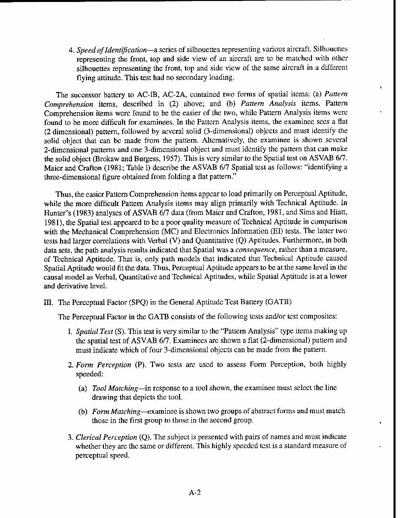
4. Speed of Identification—a series of silhouettes representing various aircraft. Silhouettes representing the front, top and side view of an aircraft are to be matched with other silhouettes representing the front, top and side view of the same aircraft in a different flying attitude. This test had no secondary loading.

The successor battery to AC-IB, AC-2A, contained two forms of spatial items: (a) Pattern Comprehension items, described in (2) above; and (b) Pattern Analysis items. Pattern Comprehension items were found to be the easier of the two, while Pattern Analysis items were found to be more difficult for examinees. In the Pattern Analysis items, the examinee sees a flat (2 dimensional) pattern, followed by several solid (3-dimensional) objects and must identify the solid object that can be made from the pattern. Alternatively, the examinee is shown several 2-dimensional patterns and one 3-dimensional object and must identify the pattern that can make the solid object (Brokaw and Burgess, 1957). This is very similar to the Spatial test on ASVAB 6/7. Maier and Crafton (1981; Table 1) describe the ASVAB 6/7 Spatial test as follows: "identifying a three-dimensional figure obtained from folding a flat pattern."

Thus, the easier Pattern Comprehension items appear to load primarily on Perceptual Aptitude, while the more difficult Pattern Analysis items may align primarily with Technical Aptitude. In Hunter's (1983) analyses of ASVAB 6/7 data (from Maier and Crafton, 1981, and Sims and Hiatt, 1981), the Spatial test appeared to be a poor quality measure of Technical Aptitude in comparison with the Mechanical Comprehension (MC) and Electronics Information (El) tests. The latter two tests had larger correlations with Verbal (V) and Quantitative (Q) Aptitudes. Furthermore, in both data sets, the path analysis results indicated that Spatial was a consequence, rather than a measure, of Technical Aptitude. That is, only path models that indicated that Technical Aptitude caused Spatial Aptitude would fit the data. Thus, Perceptual Aptitude appears to be at the same level in the causal model as Verbal, Quantitative and Technical Aptitudes, while Spatial Aptitude is at a lower and derivative level.

in. The Perceptual Factor (SPQ) in the General Aptitude Test Battery (GATB)

The Perceptual Factor in the GATB consists of the following tests and/or test composites:

1. Spatial Test (S). This test is very similar to the "Pattern Analysis" type items making up the spatial test of ASVAB 6/7. Examinees are shown a flat (2-dimensional) pattern and must indicate which of four 3-dimensional objects can be made from the pattern.

2. Form Perception (P). Two tests are used to assess Form Perception, both highly speeded:

(a) Tool Matching—in response to a tool shown, the examinee must select the line drawing that depicts the tool.

(b) Form Matching—examinee is shown two groups of abstract forms and must match those in the first group to those in the second group.

3. Clerical Perception (Q). The subject is presented with pairs of names and must indicate whether they are the same or different. This highly speeded test is a standard measure of perceptual speed.

A-2

Thus, the Perceptual Factor (SPQ) in the GATB is different from Perceptual Aptitude as found in Thorndike's (1957) AC-IB data. SPQ appears to be defined in part by a purely spatial aptitude component, and also contains a standard measure of perceptual speed based on names rather than forms. These differences may explain why the Perceptual Factor in the GATB did not appear to be a component of general mental ability, while Perceptual Aptitude did appear to be such a component in the AC-IB data.

A-3

Appendix B

Optimal Personnel Classification

B-0

Optimal Personnel Classification

The personnel classification problem is to assign people to jobs so as to maximize overall performance. The classic statement of this problem was made by Brogden (1946b). He assumed that for each job there is a known multiple regression equation for performance on that job as a function of a specific set of predictors. For example, using past validation studies, the Navy might know for each job the regression of job performance onto ASVAB aptitudes. These regression equation could be used to predict how well each recruit would do in each job. If productivity on each job were measured in the same units, recruits could be assigned to jobs where they would be most productive.

The problem is complicated by the fact that there is a quota for each job. That is, for each job there is some needed number of workers. Thus, even though all recruits might be more productive in job A, some of them must be assigned to job B. Recruits cannot simply be assigned to the job where they would be most productive. Rather, sometimes a recruit must be assigned to a job for which the loss in productivity is least

The mathematics of the classification problem is difficult and a number of papers have addressed that problem, including Brogden (1946b, 1954,1955,1964), Lord (1952), Votaw (1952) and Dwyer (1954). The key result was stated by Brogden (1954). It is possible to find a set of "adjustment coefficients" so that optimal classification is obtained when each recruit is assigned to the job with the highest adjusted productivity. To see this, consider the case of hiring. There are two "jobs": the job to be filled and the "job" of "reject." Since everyone has productivity zero if rejected, everyone would be assigned to "hire" if they were assigned to the job of highest productivity. However, if there are only 50 openings and 200 applicants, then 150 applicants must be rejected. Thus, some must be rejected even though their potential productivity would have been higher had they been hired. The optimal assignment is to reject those whose productivity would have been least. This can be done by "adjusting" performance scores in the reject condition so that selection of those with highest adjusted performance scores will place the correct applicants in the reject group. Suppose we add an adjustment coefficient to the productivity values for the reject "job." If the adjustment coefficient is large enough, there will be some workers whose performance on the job to be filled will be low enough to be lower than the adjusted value for the reject job. These will be the workers for whom there is least loss if they are assigned to the reject category. Thus, if the adjustment coefficient for the reject category is set right, then the necessary number of recruits will be assigned to that category in an optimal manner.

Brogden (1954) showed that the method of adjustment coefficients can be extended to solve the classification problem for any number of job categories. There are two parts to the solution of a classification problem. First, the problem must be stated or restated in a form so that a finite number of workers are to be placed in a finite number of jobs. Second, a method of deriving the adjustment coefficients must be developed. The procedures and computations used in this analysis are presented later in this appendix.

Validity

Validity coefficients for general cognitive ability and psychomotor ability are shown in Table 4 of the text for each of the five job complexity levels identified by Hunter (1980a). As noted in the text, this study is based on three rather than five complexity levels (e.g., see text, Table 7): High,

B-l

Medium and Low complexity. The validities at each of these three complexity levels are shown in Table B-l for (1) the current ASVAB cognitive ability, (2) ASVAB cognitive ability augmented by Perceptual Ability, and (3) Psychomotor Ability.

Table B-l

Estimated Validity of Various Ability Measures for Jobs of varying Complexity

Current ASVAB Augmented GATB Job category Cognitive ASVAB Cognitive Psychomotor

High complexity 63 .65 .21

Medium complexity -56 -58 -32

Low complexity _M .46 .43

Productivity Measurement

Most validation studies measure performance only in rank order form. For personnel selection, this poses no problem since people are usually hired into one job and the hiring decision requires only knowledge as to who is predicted to be better and who is predicted to be worse. However, for classification, performance must be compared across jobs. Thus, performance must be measured in common units. One such unit is cost. If inefficient classification causes a 10% reduction in performance in a given job, the lost production will be paid for at a rate which depends on the wage and overhead for that job. Assume, for example, that one job has a wage of $6 per hour and overhead of $4 per hour (a cost of $10 per hour total) and that a second job has a wage of $12 per hour and an overhead of $8 per hour (cost total of $20 per hour). A 10% reduction in productivity would then be twice as expensive in the second job as in the first job.

Overhead data is difficult to obtain. The average overhead level for a typical firm in the American economy is about 43% of dollar value of output (Hunter and Schmidt, 1982). If the relative overhead is about the same for all jobs, then optimal classification based on wages is optimal classification for cost as well. We make this assumption in the present analysis.

To connect validation data to cost, we need to know the cost units for each job. The mean cost for a job is given by the wage level for that job (multiplied by 1.75 to include overhead). The standard deviation of cost for jobs is not usually available from administrative records. However, there is an existing database on individual differences in productivity (Schmidt and Hunter, 1983; Hunter and Schmidt, 1987). This database contains study results showing the relationship between the mean and standard deviation of performance. The standard deviation tends to be a fixed percentage of mean performance, but that percentage varies for jobs of different complexity levels. For randomly hired applicants, the standard deviation of productivity ("ratio scale" measurement of performance) is about 25% of mean performance for low complexity jobs, about 36% for medium complexity jobs, and about 61% for high complexity jobs (though the database for high complexity jobs is thin). These percentage standard deviations translate directly into cost standard deviations once mean wage is known. The translation process is shown in Table B-2.

B-2

Table B-2

Productivi JobC

Output Standard

Deviation (%)

61

ty and Cost for Varying Levels of Complexity in the U.S. Navy

Job Category Mean Mean Wage Percentage Scale

Standard Deviation Percentage Scale

Job Characteristic

High complexity 33,073 165 101

Medium complexity 36 23,018 115 41

Low complexity 25 9,570 48 12

Reject o 0 0 0

Total 20,006 100

Distribution of People

High complexity 13

Medium complexity 62

Low complexity 15

Reject 10

Total 100

The first column of Table B-2 shows the output standard deviation for each job category as a percent of mean productivity. The second column shows mean wage for each job category. Since overhead is assumed to be proportional to wage, mean cost is proportional to mean wage. The third column rescales mean productivity so that average productivity would be 100 if applicants were randomly assigned. Note that the mean productivity includes the zero productivity of those in the reject group. The rescaled means are obtained by expressing mean wage as a percentage of the average wage of 20,006. The fourth column of Table B-2 shows the standard deviation of productivity measured on the percentage cost scale of the third column.

Quotas and the Assignment Problem

The second part of Table B-2 shows the quotas for assignment in the contemporary U.S. Navy. (These are also shown in Table 13 of the report text.) The rejection rate based on cognitive ability is 10%. The other percentages were obtained by computing the job complexity of each job in the Navy and finding the percentage of Navy personnel in each of the complexity categories, as described in the text of this report.

The classification problem for the U.S. Navy can then be stated as follows: Using known values for the relationships between ability, wage, job complexity and productivity, what is the optimum assignment of applicants to job categories using the quotas of Table B-2?

B-3

Cognitive Ability Alone

If classification is based on a single predictor, and productivity has a linear regression on that predictor, then classification takes the form of a rank order. Those applicants with the highest predictor scores are assigned to the job category with the highest raw score regression slope until that quota is filled. Those in the band below are assigned to the job with the second highest raw score slope until that quota is filled. And so on. The constant term of the regression equation does not affect assignment. In particular, differences in mean productivity do not affect optimal assignment; it is standard deviations (and validities) which determine assignments.

The average productivity of those in each band can be computed using normal curve integration. For each job category, the average predictor score for those assigned to that category is inserted into the regression equation for that category. The average productivity for all applicants is then obtained by averaging them within category averages, weighting each category mean by its quota.

Current ASVAB. The raw score regression equations for performance (P) for the best estimate of cognitive ability, using the current AS VAB, are given here with ability expressed in standard score (z-score) form:

High complexity: P = 63.4G + 165 Medium complexity: P= 23.2G+115 Low complexity: P = 5.3G + 48 Reject P = 0

The rank order of the raw regression weights is high to medium to low complexity, followed by reject. The optimal assignment is thus to assign the 13% with highest cognitive ability to high complexity work, the next 62% to medium complexity work, the next 15% to low complexity work and the bottom 10% to reject.

The mean predictor score in each category is:

High complexity: + 1.63 Medium complexity: + .17 Low complexity: - .95 Reject: - 1.76

The mean productivity is:

High complexity: 268.34 Medium complexity: 118.94 Low complexity: 42.96 Reject: 0

The average productivity across all applicants is 115.07 (vs. 100.00 for randomly assigned applicants).

B-4

Augmented ASVAB. A more valid measure of general cognitive ability can be obtained by augmenting the present ASVAB by a suitable measure of perceptual aptitude. The estimated regression equations for the augmented measure would be:

High complexity: P= 65.2G + 165 Medium complexity: P = 24.0G +115 Low complexity: P = 5.5G + 48 Reject: P = 0

The rank order of the raw regression weights is high to medium to low complexity, followed by reject. The optimal assignment is thus to assign the 13% with highest cognitive ability to high complexity work, the next 62% to medium complexity work, the next 15% to low complexity work and the bottom 10 to reject.

The mean predictor score in each category is:

High complexity: + 1.63 Medium complexity: + .17 Low complexity: - .95 Reject: - 1.76

The mean productivity is:

High complexity: 271.60 Medium complexity: 119.08 Low complexity: 42.76 Reject: 0

The average productivity across all applicants is 115.55 (vs. 100.00 for randomly assigned applicants).

Cognitive and Psychomotor Abilities In order to use Brogden's theorem to solve the classification problem for two continuously

distributed predictors, it was necessary to generate a discrete approximation. This was done by constructing 100 prototype individuals, each of whom represented 1% of the joint distribution. A computer program was then written to generate optimal classification for the prototype individuals.

Orthogonal Regression. The problem is complicated by the fact that the two predictors are correlated. The correlation between cognitive and psychomotor ability is .35. However, this complication can be avoided by transforming to mathematically equivalent predictors that are uncorrelated. Since cognitive and psychomotor ability have a bivariate normal distribution among applicants, the transformed variables will be independent.

One such transformation is to rescore psychomotor ability to generate a variable that is independent of cognitive ability. That is, the regression equations were generated for psychomotor ability with cognitive ability partialled out. If we let PA be psychomotor ability and G be general cognitive ability, the rescored psychomotor ability (PA') is given by

PA' = (PA - .35 G) / .9367 = 1.067 PA - .3736 G.

B-5

The regression equations for the orthogonalized predictors are:

High complexity: P= 66.4G + 1.0 PA + 165 Medium complexity: P= 24.0G + 5.0 PA + 115 Low complexity: P = 5.5G + 3.5 PA + 48 Reject: P = 0

Note that although the correlation between productivity and psychomotor ability is highest for low complexity jobs, the raw score regression weight is highest for medium complexity jobs.

Prototype Individuals. Since cognitive ability is uncorrelated with the rescored psychomotor ability variable, the two new predictors are independent. Thus, prototype individuals can be constructed by considering each predictor separately. The distribution of each variable was considered by deciles. Thus, there are 10 x 10 = 100 combinations of deciles across the two predictors considered jointly. The 100 prototype individuals can be considered organized in a square 10 x 10 matrix whose rows are deciles of cognitive ability and whose columns are deciles of rescored psychomotor ability (See Table 12 in text). The ability levels for each prototype individual are the mean ability levels for the 1% of the distribution which the prototype individual represents. These can be computed using normal curve integrals. For each job category, the mean productivity for the 1% class represented by each prototype individual is given by substituting the ability means for that prototype individual into the orthogonalized regression equation for that job category.

The optimal assignment problem is thus reduced to a discrete assignment problem for the 100 prototype individuals. This can be put into Brogden's form by generating a 100 x 4 productivity matrix with a row for each prototype individual and a column for each job category (counting "reject" as a job category). This was done using a computer program called JOBMAKER.

Optimal Assignment Brogden' s theorem shows that optimal assignment is obtained when optimal adjustment coefficients are obtained for each job category. There are many ways to obtain optimal adjustment coefficients. Brogden's methods were geared to hand calculations using a small number of applicants. Therefore, a new computer program called CLASSIFY was used to obtain optimal coefficients. The method used was iterative.

Brogden's theorem shows that a solution to the classification problem has been generated when one has found an adjustment coefficient for each job category such that assignment of applicants to jobs matches the given job quotas. Consider a trial set of adjustment coefficients. The adjustment coefficient for each job is added to each applicant's performance score for that job to create an adjusted performance score on that job for that applicant. Each applicant is then assigned to the job with the highest adjusted performance score. If the number of applicants assigned to each category matches the quota for that category, the assignment is optimal and the trial adjustment coefficients are one solution to the optimal assignment problem. The key to a computer program is to find an algorithm which starts with one set of trial coefficients and then generates a new set which is closer to optimum. The process can then be repeated until a set of optimal coefficients is found.

Optimal coefficients are only defined to an additive constant. That is, given one set of optimal coefficients, you can obtain an equivalent set by adding a constant to all coefficients. Thus, the coefficients can have any mean value, including zero. If one set of approximate coefficients is to be replaced by another set of coefficients with the same mean value, then the mean change in

B-6

coefficients is zero. One way to generate new estimated adjustment coefficients is to distribute change in the coefficients so that the mean change distributed is zero.

How, then, can we distribute change to the coefficients so that the new coefficients are closer to optimal than the old coefficients? We start by denning a measure of closeness to optimum. Consider a set of trial coefficients. Using those coefficients we assign applicants to jobs. We then count the number assigned to each job. The number assigned to job i can be denoted c(i). The quota for job i can be denoted q(i). The discrepancy between count and quota provides a measure of closeness to optimum for that job. Denote the signed discrepancy by d(i) (e.g., let d(i) = c(i) - q{i)). If d(i) is 0, then the count matches the quota for job i. If d(i) is positive, then we have assigned too many to job i; if d(i) is negative, then we have assigned too few to job i.

For the job as a whole, optimum assignment has been achieved only when all discrepancies are zero. A measure of overall fit would be obtained by adding the extent of discrepancy across jobs. However, we cannot add the signed discrepancies because the sum of signed discrepancies is always zero. Thus, we define the total discrepancy as the sum of the absolute discrepancies across jobs. That is, define D by

D = X\d(»\. i

Consider a set of trial coefficients. What is the relationship between the adjustment coefficient for job i and the discrepancy for job i? If we increase the adjustment coefficient, then we increase the scores for that job and we increase the number who will be assigned to that job using the new adjusted productivity scores. Since a positive discrepancy means that there are too many assigned, a positive discrepancy is a signal that we want to reduce the adjustment coefficient for that job. Since a negative discrepancy means that there are too few assigned, a negative discrepancy is a signal that we want to increase the adjustment coefficient for that job. Thus, to improve a set of adjustment coefficients, we change each coefficient by an amount opposite in sign to the sign of the discrepancy.

Suppose we have a certain total amount of change to distribute among the coefficients. How should that change be distributed? First, it seems reasonable to distribute the most change to that job with the largest absolute discrepancy. Second, the sign of the change should be opposite to the sign of the discrepancy. Let the adjustment coefficient for job i be denoted a{i). Let the total amount of absolute change to be distributed be denoted C. Both objectives can be accomplished by setting the change in coefficient a(i) to:

a(i) = w(i) C

where

w(i) = -d(i)/D.

The question on any given trial is how much change to distribute. This question can be rephrased across trials. First, how much change should we start with? Second, by how much should the amount of change be decreased on each trial? Our answer to the first question was intuitive. We set the initial amount of total change to 30 because 30 is the average standard deviation of productivity in this problem. The second question is more analytical in form. As the trial fit gets closer, the amount of change should decrease. In our program, we simply decreased the amount of

B-7

change in proportion to the decrease in total discrepancy. For example, if a given trial caused D to decrease by 50%, then C would also decrease by 50%.

There can be two problems with change: too much or too little. If there is too much change, the process can overshoot. Overshoot can usually be detected by observing the pattern of the signs of the discrepancies. Overshoot usually causes all or most discrepancies to reverse sign. This kind of overshoot can usually be cured by cutting the amount of change in one half.

Can there be too little change? In some iteration processes, it is possible for the change to decrease to zero before the process reaches a solution. This is not possible in our program. Consider an amount of change so small that all applicants are assigned to the same jobs. The discrepancies will be unchanged, the total discrepancy will be unchanged, and hence the amount of change will not decrease. Thus, over a period of n such trials, the total amount of change will be n times the amount on a single trial. Thus, there will always eventually be enough change to cause an applicant to shift categories.

On the other hand, such change can be very slow. If the program is run on an interpreter and the results are printed to the screen on each trial, the operator can detect such slow change directly. The operator can then interrupt the program, double (or triple or more) the current amount of change, and resume computing. This was not needed for the present research.

The speed of an iterative procedure depends on the initial trial values. The closer the initial values, the quicker the process converges. The present program sets the initial trial adjustment coefficients at zero. This is very inefficient, especially for the reject category. The coefficient for the reject category had a long way to rise until 10% of the prototype individuals had adjusted scores higher than those in the productive job categories. If the predictors are measured as standard scores, a better set of initial coefficients would be chosen to eliminate the effect of the regression constant terms. For example, if the regression constant term for job i is b(i), then a reasonable initial value for the adjustment coefficient would probably be -b(i).

B-8

Distribution List

Distribution: Office of the Assistant Secretary of Defense (P&R) (2) Office of the Assistant Secretary of Defense (FM&P) Defense Technical Information Center (DTIC) (4)

Copy to: Pentagon Library Deputy Chief of Naval Operations (M&P) (Nl) Assistant Deputy Chief of Naval Operations (NIB) Office of the Director, Test and Evaluation and Technology Requirements (N091) Director, Chief of Naval Research (Code 01) Director, Technology Directorate (Code 04) Director, Personnel/Training and Human Factors Division (Code 461) Chief of Naval Education and Training (L01) (2) Assistant for Planning and Technical Development (PERS-01JJ) Public Affairs Office (PERS-05) Director, Recruiting and Retention Programs Division (PERS-23) Director, Research and Development Department of Defense Coordinator (PERS-234) (3) Head, Fiscal Management Branch (PERS-463) Commanding Officer, Naval Aerospace Medical Research Laboratory, Pensacola, FL Commandant of the Marine Corps Commander, U.S. ARI, Behavioral and Social Sciences, Alexandria, VA (PERI-POT-I) Director, U.S. ARI, Behavioral and Social Sciences, Alexandria VA (PERI-ZT) AISTA (PERI II), ARI Armstrong Laboratory, Operations and Support Directorate (AL/DO), Brooks, AFB, TX AL/HR-DOKL Technical Library, Brooks, AFB, TX Superintendent, Naval Postgraduate School Director of Research, U.S. Naval Academy Program Manager, Manpower Research and Advisory Service, Smithsonian Institution Institute for Defense Analyses, Science and Technology Division Center for Naval Analyses, Acquisition Unit Center for Naval Analyses Systems Research Center, Virginia Tech., Blacksburg, VA