runtime service composition via logic-based program synthesis
TRANSCRIPT

Runtime Service Composition via Logic-Based Program Synthesis
Sven Lämmermann
A dissertation submitted to the Royal Institute of Technology in partial fulfillment of the requirements for the degree of Doctor of Philosophy
June 2002
TRITA-IT AVH 02:03 ISSN 1403-5286 ISRN KTH/IT/AVH 02/03–SE
Department of Microelectronics and Information Technology Royal Institute of Technology Stockholm, Sweden

Author’s e-mail address: [email protected]
Department of Microelectronics and Information Technology Royal Institute of Technology Electrum 229, 16440 Kista (Stockholm), Sweden
© Sven Lämmermann, 2002

Abstract Dynamic composition of services from components at runtime can help to provide flexible service infrastructures, but requires advanced composition techniques. To address this problem, we have developed a composition method that is tailored to services. The method integrates an efficient deductive program synthesis technique with a specification language. The work is realized in the context of an object-oriented software platform. The platform introduces a declarative extension to an object-oriented programming language in order to combine advantages of object-oriented programming with positive sides of declarative programming. We introduce the notion of declarative service programming. The declarative part uses the extended structural synthesis of programs, which we have developed. The extended structural synthesis of programs is an extension of the structural synthesis of programs (SSP). In contrast to the original SSP, our extensions allow program composition for dynamic environments. In pure SSP, the context in which components are used has to be specified in advance, i.e. statically. Service configurations are represented as classes and interfaces. We introduce metainterfaces as logical specifications of classes. They can be used in two ways: as specifications of computational usage of classes or as specifications of new classes composed from classes already supplied with metainterfaces. A metainterface is a specification that 1) introduces a collection of interface variables of a class, 2) introduces axioms showing the possibilities of computing provided by methods of the class, in particular, which interface variables are computable from other variables under which conditions, and 3) introduces metavariables that connect implicitly different metainterfaces and reflect on the conceptual level mutual needs of components. Our aim in designing the specification language has been to make it as convenient as possible for a software developer. This language allows a simple and exact translation into the language of logic used by the synthesis process, but we have tried to avoid excessive use of logical notations. We have implemented a prototype for automated compositional synthesis. It has been used in several experiments to show the feasibility of fully automated service composition. We describe some service composition examples. We present performance measurements of service compositions involving large number of component specifications. Our prototype implementation has shown good synthesis performance for services occurring in practice.


Acknowledgements This thesis is the result of my research at KTH during the period January 1998 − December 2001. The support I have received from KTH and PCC project financially in the form of a PhD student scholarship is herewith thankfully acknowledged. I am grateful to my supervisor Prof. Enn Tyugu for the time he invested in advising me as well as for his encouragement. I also benefited much from discussions with Tarmo Uustalu. He was particularly helpful in explaining the structural synthesis of programs to me and was a wonderful source of the kind of information logicians don't write about because they assume everyone already knows it. I would like to thank Prof. Grigori Mints, who helped me to take my first steps in logic during a course given at the former Department of Teleinformatics in 1998. Thanks to Vladimir Vlassov, who has given advice and encouragement. Thanks to Prof. Seif Haridi who always has had an open ear for any problem. It is also a pleasure to record my appreciation of the help I have received from Hans Holmberg, Rita Johnsson, Rita Fjällendahl, Agneta Herling, Hans-Jörgen Rasmusson and the late Barbro Persson. I am, of course, also grateful to Bernd Fischer from NASA Ames Research for reviewing this dissertation and for his kind promise to serve as the opponent at the defence event. His comments significantly improved the technical content. To Ian Marsh from SICS, I owe thanks for proofreading this thesis and suggesting improvements to the language. Finally, I would like to thank my family, especially my dear wife Beatrice and my sons Patrice Noel and Pascal Christophe for their endurance and encouragement.
Sven Lämmermann Stockholm June 2002


To Beatrice


C o n t e n t s
List of Tables xv
List of Figures xvi
1 Introduction 1 1.1 Background.................................................................................................. 2 1.2 Motivation ................................................................................................... 3
1.2.1 Service Composition...................................................................... 3 1.2.2 Composition Languages ................................................................ 4 1.2.3 Program Synthesis ......................................................................... 4
1.3 Problem Statement....................................................................................... 5 1.3.1 Service Composition from Components ........................................ 5 1.3.2 Specification Language ................................................................. 6 1.3.3 Implementation.............................................................................. 7
1.4 Proposed Solution........................................................................................ 7 1.4.1 Automated Service Composition ................................................... 8 1.4.2 Specification Language for Services and Components.................. 8
1.5 Contributions ............................................................................................... 9
ix

CONTENTS x
1.6 Outline ....................................................................................................... 11
2 Services and Runtime Service Composition 13 2.1 Introduction................................................................................................ 13 2.2 Traditional Services ................................................................................... 14 2.3 Runtime Service Composition: Why?........................................................ 15
2.3.1 Interoperability ............................................................................ 16 2.3.2 Platform Independence ................................................................ 17 2.3.3 Active Networks .......................................................................... 17
2.4 Runtime Service Composition: How?........................................................ 18 2.4.1 Service Components .................................................................... 19 2.4.2 Service Component Specification................................................ 20 2.4.3 Service Composition.................................................................... 21
2.5 Sample Application.................................................................................... 21 2.6 Requirements for Runtime Service Composition ...................................... 23
3 A Calculus for Runtime Service Composition 27 3.1 Preliminaries .............................................................................................. 28
3.1.1 Intuitionistic Logic....................................................................... 28 3.1.2 Natural Deduction........................................................................ 29 3.1.3 Intuitionistic Natural Deduction .................................................. 30
3.1.3.1 Inference Rules .............................................................. 31 3.1.3.2 Localizing Hypotheses................................................... 36 3.1.3.3 Structural Properties of Hypothesis ............................... 37 3.1.3.4 Proof Terms ................................................................... 38
3.1.4 Derivation Example and Program Extraction from Proofs .......... 40 3.2 Structural Synthesis of Programs............................................................... 41
3.2.1 Logical Language LL ................................................................... 42 3.2.2 Inference Rules ............................................................................ 44 3.2.3 Completeness of LL ..................................................................... 45 3.2.4 Program Extraction...................................................................... 46

CONTENTS xi
3.2.5 Structural Synthesis Rules ........................................................... 47 3.2.6 Program Extraction for Structural Synthesis Rules ..................... 49 3.2.7 Example of a Proof with Program Extraction.............................. 49 3.2.8 Dependent and Independent Subtasks ......................................... 50 3.2.9 Proof Search Algorithm............................................................... 51 3.2.10 Branch Control Structures in SSP................................................ 54
3.3 Extended Structural Synthesis of Programs............................................... 55 3.3.1 Logical Language LL of ESSP..................................................... 57 3.3.2 Inference Rules ............................................................................ 58 3.3.3 Program Extraction...................................................................... 59 3.3.4 Structural Synthesis Rules (ESSP) .............................................. 60 3.3.5 Program Extraction for Structural Synthesis Rules (ESSP)......... 62 3.3.6 Proof Search Algorithm Extension for Disjunction..................... 63 3.3.7 Proof Search Algorithm Extension for Quantifier Elimination ... 65 3.3.8 Example of Synthesis with Program Extraction .......................... 66
4 Specification Language 69 4.1 Core of the Language................................................................................. 70
4.1.1 Interface Variables....................................................................... 70 4.1.2 Constants ..................................................................................... 71 4.1.3 Bindings....................................................................................... 71 4.1.4 Axioms ........................................................................................ 72 4.1.5 Implemented Axioms................................................................... 74 4.1.6 Unimplemented Axioms .............................................................. 75 4.1.7 Subtasks ....................................................................................... 75 4.1.8 Dependent Subtasks..................................................................... 76 4.1.9 Independent Subtasks .................................................................. 76 4.1.10 Goals............................................................................................ 77
4.2 Language Extensions ................................................................................. 77 4.2.1 Metavariables............................................................................... 78

CONTENTS xii
4.2.2 Control Variables......................................................................... 81 4.3 Logical Semantics...................................................................................... 82
4.3.1 Unfolding..................................................................................... 82 4.3.2 Structural Properties .................................................................... 83 4.3.3 Instance Value ............................................................................. 84 4.3.4 Logical Semantics of Metainterfaces........................................... 84
5 Synthesis 89 5.1 General Scheme of Synthesis..................................................................... 89 5.2 Synthesizing a Service Component ........................................................... 90 5.3 Synthesizing a Service ............................................................................... 95
6 Application to Java 101 6.1 Introduction.............................................................................................. 101 6.2 Adding Specifications to Classes............................................................. 102
6.2.1 Connection between Class and Metainterface ........................... 103 6.2.2 Interface Variables..................................................................... 103 6.2.3 Constants ................................................................................... 105 6.2.4 Metavariables............................................................................. 106 6.2.5 Bindings..................................................................................... 107 6.2.6 Subtasks ..................................................................................... 108 6.2.7 Axioms ...................................................................................... 113 6.2.8 Using Control Variables ............................................................ 115 6.2.9 Exceptions ................................................................................. 117 6.2.10 Falsity ........................................................................................ 121 6.2.11 Inheritance ................................................................................. 123 6.2.12 Overriding.................................................................................. 124 6.2.13 Overloading ............................................................................... 125
6.3 Program Extraction.................................................................................. 125 6.4 Synthesis of Java Programs ..................................................................... 126 6.5 Performance of Synthesis ........................................................................ 128

CONTENTS xiii
6.5.1 Environment .............................................................................. 128 6.5.2 Test Set ...................................................................................... 128
6.5.2.1 Synthesis Problems...................................................... 128 6.5.2.2 Synthesized Programs.................................................. 131 6.5.2.3 Hand-coded Programs ................................................. 132
6.5.3 Expected Results........................................................................ 133 6.5.4 Measurements ............................................................................ 133 6.5.5 Analyses..................................................................................... 134
7 Application to Runtime Service Composition 137 7.1 A Print Service......................................................................................... 138 7.2 Stock Quote Cache................................................................................... 142 7.3 Summary.................................................................................................. 146
8 Concurrent Implementation of Synthesized Services 147 8.1 Multithreaded Execution of a Synthesized Program................................ 148 8.2 Implementation in Java............................................................................ 150 8.3 Coarse-Grained Parallelization ................................................................ 153
8.3.1 Composing Threads ................................................................... 154 8.3.2 Imposing Parallelism on Subtasks ............................................. 154
8.4 Summary.................................................................................................. 155
9 Related Work 157 9.1 Program Synthesis ................................................................................... 157
9.1.1 Transformational Approach....................................................... 158 9.1.2 Inductive Approach ................................................................... 159
9.2 Deductive Program Synthesis .................................................................. 160 9.2.1 Deductive Program Synthesis Methods ..................................... 160 9.2.2 The Amphion System ................................................................ 163 9.2.3 The NUT System ....................................................................... 163 9.2.4 Amphion vs. NUT ..................................................................... 163

CONTENTS xiv
9.2.5 KIDS.......................................................................................... 164 9.2.6 Planware .................................................................................... 164
9.3 Software Composition Languages ........................................................... 164 9.3.1 Coordination Languages ............................................................ 166 9.3.2 PICCOLA .................................................................................. 168
9.4 Service Composition................................................................................ 170 9.4.1 A Reuse and Composition Protocol........................................... 171 9.4.2 Hadas ......................................................................................... 171 9.4.3 Adaptive and Dynamic Service Composition in eFlow............. 171 9.4.4 The Aurora Architecture............................................................ 171
10 Conclusion and Future Work 175 10.1 Concluding Remarks................................................................................ 175 10.2 Future Work............................................................................................. 177
10.2.1 Integrating Component Selection and Adaptation ..................... 177 10.2.2 Distributed Runtime Service Composition ................................ 177
Bibliography 179

CONTENTS xv
List of Tables
Table 1 Inference rules of intuitionistic propositional natural deduction................ 35 Table 2 Localized version of inference rules .......................................................... 37 Table 3 Inference rules using proof terms .............................................................. 40 Table 4 Conventional inference rules (SSP) ........................................................... 44 Table 5 Conventional inference rules using proof terms (SSP) .............................. 46 Table 6 SSR using proof terms (SSP)..................................................................... 49 Table 7 SSR for planning with independent subtasks............................................. 51 Table 8 Conventional inference rules (ESSP)......................................................... 58 Table 9 Conventional inference rules using proof terms (ESSP)............................ 60 Table 10 SSR using proof terms (ESSP) .................................................................. 63 Table 11 Inheritance in metainterfaces ................................................................... 124

CONTENTS xvi
List of Figures
Figure 1 Web cache of active network node ......................................................... 22 Figure 2 Web and stock quote cache of active network node ............................... 23 Figure 3 Search tree to example double integration .............................................. 52 Figure 4 HODS to example double integral .......................................................... 53 Figure 5 Components before and after synthesis to example print service ........... 56 Figure 6 Search tree with innermost goals to example double integration............ 64 Figure 7 General scheme of service synthesis....................................................... 90 Figure 8 Pseudo-proof to example exchange rate.................................................. 95 Figure 9 Pseudo-proof to example bank................................................................ 98 Figure 10 Extracted program (pseudo-code) ........................................................... 99 Figure 11 Java program code to illustrate double integration ............................... 112 Figure 12 Java code for java.rmi.Naming.lookup.................................... 118 Figure 13 Specifying a new Java program ............................................................ 127 Figure 14 Steps of synthesis process ..................................................................... 127 Figure 15 Performance measurements .................................................................. 134 Figure 16 Java program to illustrate the print service ........................................... 140 Figure 17 Java program that uses the synthesized print service ............................ 141 Figure 18 Java program to illustrate the stock quote cache................................... 145 Figure 19 Steps of conventional structural synthesis of programs ........................ 148 Figure 20 Steps of structural program synthesis using guarded threads................ 150 Figure 21 Higher-order dataflow schema.............................................................. 153 Figure 22 Composing threads................................................................................ 154 Figure 23 Parallelism in control node ................................................................... 155

Chap t e r 1
Introduction
This thesis discusses service composition at runtime, i.e. for the cases when the actual service program does not exist before service request. A program to provide a particular service is composed in the user interaction loop on the basis of a service request that specifies this service. But this thesis work concentrates on fully automated efficient program synthesis, which is a precondition to put runtime service composition into praxis. This is particularly the case if logic-based program synthesis is used, because pure logic-based program synthesis is in general difficult to apply in practice. It can be time-inefficient because it may require expensive theorem proving tasks due to the expressiveness of logical languages.
We report an approach to fully automated service composition. It involves an efficient program synthesis method, which we have extended with more complex specification possibilities needed for composing service programs at runtime, and a specification language for service components. We present an application to service program composition.
In this introductory chapter, we explain what provoked our interest in the subject, describe our contribution and present the organization of the thesis.
1
Chapter 1 Introduction 2
1.1 Background
The last few years have seen continued growth in the size and complexity of service systems at the same time that reliance on their operation has increased. As service platforms evolve from separate back-office and personal systems providing limited service support, to pervasive networked service environments providing electronic services where communication of different systems is involved, service technologies become increasingly complex and critical. Shutting down a running system is economically not justifiable.
The requirements for maintaining complex service systems to provide reliable services necessitate careful design and development of all of the components involved in electronic service systems. An ideal infrastructure for services would provide modular structures and dynamic composition so that services can be easily added, modified, and removed with low (preferable zero) impact on the existing service components and the rest of the system. Service engineering is a discipline that addresses these issues. It involves the definition and development of software infrastructures for services (Trigila et al. 1995).
Dynamic composition of service applications from components at runtime is becoming attractive, and requires advanced composition techniques. Several systems have been proposed and successfully shown to provide flexibility. Those systems involve languages for software composition and coordination. Scripts written in those languages link components explicitly but establish communication channels among them dynamically. Composition scripts can provide flexibility because they are easily exchangeable.
Scripts are, however, static structures specifying certain compositions explicitly. Hence, automated adaptation to changing user requirements cannot be provided. With automated adaptation we mean automated recomposition of service programs according to users' needs in a particular situation. A typical example from the mobile computing domain is the printer problem. Assume we want to print a document whose format does not match the format required by the printer or we use software that does not support the print protocol of the printer server. In such a situation, an experienced user tries to identify executable components (tools) that in composition help to overcome the printer problem, i.e. composition of a service program that is tailored to this particular situation. Those compositions are typical for UNIX environments; using a scripting language configures the composite service.
In this thesis we show how a specification language and constructive logic can be used to provide services that can adapt if requirements change. We focus on a composition method for service applications, which are put together from pre-programmed service components. We define a service component (we write component if it cannot cause any confusion) as a pre-programmed function or method, which is a black box that provides some service and may require other services at the same time. We say a service component is configurable if it requires

1.2 Motivation 3
services. Every service component has a logical description that specifies the compositional properties and the behavior of the component. A program to provide a particular service is composed in the user interaction loop on the basis of a service request that specifies this service.
1.2 Motivation
We are interested in the questions of how to fully automate service program composition at runtime and how this can serve to provide flexible and adaptive services and at the same time increase software maintainability and reuse. When choosing the subject for this thesis, three research directions inspired us. First of all, we were inspired by research on dynamic composition of services, i.e. software infrastructures that support on-demand composition of services, which involves identifying components at run-time and dynamically establishing communication channels among them, so that they can interact. Second, we were inspired by research on deductive program synthesis using the intuitionistic propositional calculus, and third, by research on software composition languages.
1.2.1 Service Composition The concept of software component composition is fundamental to software engineering. Software components are black-box entities. They implement abstractions and can be used to effectively construct complex software systems. Software component composition is also important to dynamic service composition. The main focus of research of service composition has been providing frameworks, architectures, and methodologies to help service designers to create useful, reusable, and maintainable services. We are convinced that service composition from components is the only realistic approach to meet future requirements on services.
Traditional service composition assumes applications mostly executed in a predictable, static, and repetitive way. On the contrary, composite services are intended to execute in dynamically changing environments. They have to cope with frequent service recomposition to address new requirements. One of such dynamically changing environments is the Internet where new services become available on a daily basis. Another example is intra-nets of companies that use a variety of different tools providing services for particular purposes. Integrating those tools to solve larger problems turns out to be a very hard task and can hardly be carried out automatically.
Currently, we see a trend away from traditional service composition, where services composed from components are compiled into static monoliths, to dynamic service composition, where a requested service is realized by dynamically establishing communication channels between components according to some service flow specification.

Chapter 1 Introduction 4
1.2.2 Composition Languages Object-oriented programming languages, for instance, are well suited to implement software components, but construction of component-based applications appears to be difficult. This is because object-oriented software design has a tendency to complicate a component-based architecture (Nierstrasz and Meijler 1994). To tackle this problem researchers propose to clearly separate component implementation and composition, where composition rules are specified by a specific software architecture.
A software architecture describes the assignment of functionality to components, and the interaction among components. Languages for software composition should support the description of software architectures at a sufficiently high level of abstraction, i.e. making the architecture of an individual application explicit (Magee, Dulay, and Kramer 1995).
In the literature (see for instance Achermann et al. 2000) a composition language is described as a combination of the following aspects: a) architectural description, allowing to specify and reason about component architectures, b) scripting, allowing to specify applications as configurations of components according to a given architectural style1, c) glue, enabling component adaptation, and d) coordination, needed to specify communication coordination mechanisms and execution policies for concurrent and distributed components.
All of these four aspects have been studied for many years and implemented in different languages, each emphasizing one of these aspects. For instance, Linda (Carriero and Gelernter 1989) is a language used for coordination and Perl (Wall, Christiansen, and Schwartz 1996) is a typical scripting language used for application configuration.
A composition language can be used to specify compositions explicitly, or it can be used for writing a declarative specification of a composition so that a software application will be generated automatically. The advantage of specifying compositions explicitly is that it gives us the best control, and enables us to specify more sophisticated compositions, but a disadvantage is that it yields a static structure whose implementation cannot change without user-system interaction. Using declarative specification of a composition gives us flexibility and adaptation in terms of a composite software application whose implementation can change as conditions imposed by the environment and user change.
1.2.3 Program Synthesis Program synthesis is a method of software engineering used to generate programs automatically. Usually three different approaches to program synthesis are 1 An architectural style or component architecture defines the plugs, the connectors, and the
corresponding composition rules for components.

1.3 Problem Statement 5
distinguished. These are transformational, inductive, and deductive program synthesis (Rich and Waters 1986). (We briefly discuss them in section 9.1.) We believe that a fully automated deductive program synthesis method serves best for runtime service composition. Deductive techniques have the valuable property that a program's specification that represents a relationship between a given input and the desired output, expressed in logic, can be phrased as a theorem that states the existence of an output that meets the specified conditions. The theorem must be proved automatically and constructively. The generated proof becomes the basis for a correct program that can be extracted from the proof, because the proof shows that the extracted program does meet its specification.
1.3 Problem Statement
Providing flexible and adaptive services requires combining existing components into one service dynamically, and configuring components to specific requirements. Proposed approaches to dynamic service composition are most often either rule-based or coordination language based systems that require user-system interaction for service reconfiguration whenever conditions imposed by the environment or user change. Maintaining flexibility and adaptation of services provided by these techniques requires service monitoring and frequent service reconfiguration by manual coding. The problem of providing an efficient method for fully automated service composition, which should provide flexibility and adaptation, manifests itself directly in the cases of service component specification and composition.
1.3.1 Service Composition from Components To scale up service composition to large component libraries and to provide flexibility, component selection and composition must be efficient, and component specification must be kept easily comprehensible. It is a strong requirement that an appropriate automated service composition method must yield correct service programs with respect to their respective specifications. Unpredictable component application, as in case of rule-based systems if no inference is applied, is not acceptable.
We can reduce the problem of service composition at service request to the following. Interfaces are entry points to services that are non-changeable at runtime. A service request must match a certain service interface. Interfaces of components (which can also be services themselves) do in general not tell us anything about their composability. Hence, automated service composition cannot be supported without reasoning about component interfaces automatically.
We believe that advanced logic-based program synthesis techniques can help to provide automated reasoning about component interfaces. Logic-based program synthesis uses a logical proof that guarantees correct deployment of components in

Chapter 1 Introduction 6
the context of their use, but only if the context is sufficiently represented in the logic (in the specification).
It is also our goal to select a set of potential components from a pre-described component library during service composition, using the semantics of the components and the service specification that is given by a service request. Component selection often requires component adaptation (Penix and Alexander 1997), or that multiple components will be combined into a component that solves the problem (Penix 1998).
The composition method must not significantly affect service response latency, which can be achieved only by using a time efficient synthesis algorithm as the one used in structural synthesis of programs (Mints and Tyugu 1982).
1.3.2 Specification Language In order to provide automated service composition we need a specification language that enables us (i) to specify components, (ii) to specify the context of component usage, and (iii) to write goals that specify desired service programs. We distinguish between two languages, a specification (user) language and a logical language. Specifications written in the user language are translated into the logical language. The user language is a macro language on top of the logical language. It is designed to write specifications in the problem domain. Logical details are hidden from the user, although they are reachable, if needed. We believe that a user specification language on top of a logical language enhances accessibility in the sense that knowledge can be represented in a convenient way, because the user language is designed for the problem domain. We also think that a user language helps to increase on confidence that a written specification means what the user wants to express, because the user is forced to write specifications in a certain way. More importantly, a user language can be defined on a restricted subset of the underlying logical language. The restricted subset can have better properties, e.g., complexity.
A service component is a physical encapsulation of some functionality of service according to a published specification. A component specification is given by a description of the syntactic interface and a logical formula that relates input and output (Broy 1997). Specification languages should be suitable for evaluating component reusability, but may require expensive theorem proving tasks because of their expressiveness, which in turn limits their usefulness as a component selection mechanism.
Since component selection represents a crucial factor for a composition mechanism and it is strongly related to the complexity of the underlying specification language, we need to find a feasible balance between expressiveness and efficiency of the specification language that is suitable for service composition at runtime.
We also need to be able to specify properties and behavior of components in a reasonable easy way, but the specification language must still allow to reason about components automatically according to our needs. A suitable component specification

1.4 Proposed Solution 7
language must be expressive enough for describing, first, the structure of hierarchical configurations appearing in services, and second, dataflow between components. It must have a precise semantics.
1.3.3 Implementation As this work has been performed in the context of a larger project (Personal Computing and Communication (PCC)), we had the practical goal to implement our technique to justify our approach. We have decided to implement our domain-independent program synthesis technique in an object-oriented programming language, namely Java. We extend Java classes with a declarative part. The declarative part is supported by the program synthesis technique. We have chosen Java because it is a widely used object-oriented language that is suitable for implementing services in a network. Components of services are represented as classes. Moreover, Java supports well class introspection through reflection tools, which facilitates program code generation and enabled us to keep the specification (user) language small.
The implementation of our service composition system is directly suggested by the general scheme of synthesis, which we discuss in Chapter 5. The scheme of synthesis involves three levels, which are: 1) level of specification (user) language, 2) level of logical language, and 3) level of programming language. Each level is implemented as separate module. The first level translates source specifications (written in the user language) into the logical language (i.e., into the specific axioms of a formal theory). The formal theory is used to prove the existence theorem for a given service specification. This is implemented as a theorem prover on the second level. Output of the theorem prover is an abstract syntax tree (Batory, Lofaso, and Smaragdakis 1998) representing an algorithm if the given service specification has a realization. On the third level, we generate executable program source code for the target programming language from the abstract syntax tree. The move from level one to level two is an essential feature of the proposed service composition method. It allows us to flatten hierarchical service component specifications without loss of information, which in turn allows efficient proof search.
1.4 Proposed Solution
To address these problems, a component composition method that is tailored to services has been developed. The method integrates an efficient deductive program synthesis technique with a specification language to provide efficient service composition. The work is realized in the context of an object-oriented software platform. Developing a prototype of this platform constitutes an essential part of the presented thesis work. The prototype introduces a declarative extension to an object-oriented programming language in order to combine advantages of object-oriented
Chapter 1 Introduction 8
programming with positive sides of declarative programming, which introduces the notion of declarative service programming. The declarative part uses the extended structural synthesis of programs. The usage of an object-oriented programming language turns out to be most suitable because of composition mechanisms such as inheritance and aggregation, which are needed for service configuration.
Unlike the traditional imperative way of service programming, declarative service programming does not require explicit instructions of how a particular service has to be realized, and there is nothing in specifications that corresponds to program control structures. This is similar to logic programming languages such as Prolog (Spivey 1996). The absence of explicit instructions is one of the attractions of a declarative style of service programming that gives us a high degree of flexibility. It is comparatively easier to substitute, add, remove, or update a service specification than to modify program code that in turn might require changes of other parts of the program.
1.4.1 Automated Service Composition In our case, a service request is a query that specifies the requested service. Based on this service specification and the specifications of the components in the component library, an inference system tries to prove that there exists a program that satisfies the service specification. If there exists such a program then this program must be a realization of the requested service. The proof of existence of requested service is constructive and gives the basis for service program extraction from this proof. That gives us flexibility and adaptation in terms of a service whose realization can change as conditions imposed by the environment and user change.
We use an efficient program synthesis method that is an extension of the structural synthesis of programs (SSP) (Mints and Tyugu 1982). The synthesis method is based on the semantics provided by formal component specification. Our method embodies theoretical developments stemming from the SSP and NUT (Tyugu 1994). In contrast to the original SSP, our extensions allow program composition for dynamic environments. In pure SSP and systems such as NUT, the context in which components are used has to be specified in advance.
1.4.2 Specification Language for Services and Components Using components is one of the most prevalent forms of software reuse. It involves finding all appropriate components and then designing the interface code that matches the components to the context of their use. Finding appropriate components is often a very difficult and time-consuming task for programmers. Composing components appropriate to an application turns out to be another problem requiring expertise of users. In domains with mature subroutine (or class) libraries, software development can be improved by automating the use of those libraries (Biggerstaff and Perlis 1989).
1.5 Contributions 9
Information about particular service is information about 1) computability, 2) required resources, and 3) requirements for using components. This information can be represented as a specification related to a location. It should be encoded in logic to be used for automated composition of services.
We have chosen an object oriented programming language (namely Java) that we extend with a declarative part. Service configurations and components are represented as classes and interfaces. We introduce metainterfaces as logical specifications of classes. They can be used in two ways: as specifications of computational usage of classes or as specifications of new classes composed from classes already supplied with meta-interfaces. A metainterface is a specification that: 1) introduces a collection of interface variables of a class, 2) introduces axioms showing the possibilities of computing provided by methods of the class, in particular, which interface variables are computable from other variables under which conditions, and 3) introduces metavariables that connect implicitly different metainterfaces and reflect on the conceptual level mutual needs of components.
Our aim in designing the specification language has been to make it as convenient as possible for a software developer. This language allows a simple and exact translation into the logical language used by the synthesis process, but we have tried to avoid excessive use of logical notations. The following design decisions have been made. We have separated interface variables from instance and class variables. This gives flexibility to specifications and enables us to specify existing classes developed initially without considerations about their appropriateness for synthesis. Moreover, by separation of interface variables from attributes of metaclasses the creation of new side effects is avoided. Inheritance is supported in specifications. This may cause inconsistencies if an implementation of some relation is overridden. Fortunately, this situation can be detected automatically by introspection of classes.
1.5 Contributions
We propose to use a formal program synthesis method and formal specification language for services and components that in combination yield an efficient method for service composition at runtime. The program synthesis method uses a constructive logic that is expressive enough for describing, first, the structure of hierarchical configurations appearing in services and, second, dataflow between components. The proposed approach to fully automated service composition is based on the fact that most services can be modeled as a set of components that are connected through dataflow dependencies.
This work makes the following contributions in the application of formal methods to support open services:
1. Development and application of a formal method for fully automated program synthesis to enable efficient program composition without user-

Chapter 1 Introduction 10
system interaction (Chapter 3). The proposed program synthesis method is an extension of the structural synthesis of programs (SSP) by Mints and Tyugu. We present several extensions of the logical language that are needed for more complex specification possibilities. We also present extensions of the proof search algorithm.
2. Development of a specification language for services and preprogrammed components to enable automated reasoning about components (Chapter 4 and Chapter 5). The specification language allows supplying components with specifications in a reasonably easy way, so that the semantics of a specification can be understood immediately. The semantics of the language is presented by mapping its statements to the language of our logic. We introduce the notion of metaclasses and metainterfaces, which operate on compositional level. We also introduce the notion of metavariables. We show how metavariables can be used to implicitly specify dataflow dependencies among autonomous components to overcome composition limitations. An object-oriented programming language has been extended with our specification language. Specifying properties of classes by supplying methods of classes with specifications fits very well into the object-oriented programming paradigm and provides component specification and composition mechanisms at the same time.
3. Feasibility demonstration of fully automated composition of services (Chapter 6 and Chapter 7). In Chapter 2 we present a study of services, and in particular their properties in terms of decomposability. Conclusions of this chapter are reused in Chapter 7 for a feasibility demonstration. We have implemented a prototype for automated compositional synthesis. It has been used in several experiments to show the feasibility of fully automated service composition. We present several service composition examples. Feasibility is also demonstrated by performance measurements of compositions involving large number of component specifications.
4. Development of a method for introducing concurrency into structurally synthesized service programs (Chapter 8). Open and distributed service environments involve concurrent execution of service programs. The specifications for structural synthesis of programs contain information needed for introducing concurrency into a composed program. We studied how this can be used in a multithreaded computing environment. We propose strategies of coarse-grained multithreaded execution of composed programs: composing threads and imposing parallelism on subtasks. We introduce the notion of environment of tuples, which is similar to tuple spaces in Linda.
1.6 Outline 11
1.6 Outline
This thesis is organized as follows. Chapter 2 is dedicated to a study of services and automated composition; in particular we discuss informally properties of services in terms of composability. We define components and composition in terms of services, and introduce the notion of runtime service composition. We also present requirements for runtime service composition. In Chapter 3 we first introduce briefly some of the main formalisms of natural deduction, intuitionistic natural deduction, proofs, and proof terms. This section of Chapter 3 has to be considered as a preparatory section to understand the fundamentals of the proposed composition method and gives a theoretical basis. After these preliminaries we give an introduction to the structural synthesis of programs (SSP). Then, the extensions to the SSP will be presented. An explanation of the extended proof search algorithm follows. In Chapter 4 we develop a specification language for service components. Formal semantics of the language is presented. Our general scheme of synthesis is presented in Chapter 5. Chapter 6 describes the application to Java and extending classes with a declarative part. We also discuss performance measurements of compositions involving large numbers of component specifications. A feasibility demonstration of fully automated composition of services is presented in Chapter 7. We show two service composition examples. Open and distributed service environments involve concurrent execution of service programs. We describe a method for introducing concurrency into structurally synthesized service programs in Chapter 8. We present strategies of coarse-grained multithreaded execution of composed programs and introduce the notion of execution environments of guarded threads. Chapter 9 surveys published work that bears a relation to our work. The survey is divided into four sections. We start with related work on program synthesis and deductive program synthesis. Thereafter we discuss software composition languages, where we focus on coordination languages and scripting languages. We discuss a framework for developing network-centric applications by dynamic composition of services. In Chapter 10 we present conclusions and propose further work.

Chap t e r 2
Services and Runtime Service Composition
In this section we discuss services and automated composition of (distributed) services; in particular we consider properties of services in terms of decomposability. We define components and composition with respect to services and distributed computing, and we introduce the notion of runtime service composition. The questions of why runtime service composition is needed and how it can be provided will be answered. We also present requirements for runtime service composition methods.
2.1 Introduction
We believe that on-the-fly composition of services from components is becoming attractive, but requires advanced composition methods. Composability, configurability, and extensibility of services provided by interconnected computer systems and their implementations have recently been the targets of active research efforts (Nikolaou, Marazakis, and Papadakis 1998, Beringer, Wiederhold, and Melloul 1999, Casati et al. 2000, Ben Shaul, Gidron, and Holder 1998, Mennie and Pagurek 2001, Mennie and Pagurek 2000, Fuentes and Troya 1997). For various reasons, many research contributions are contributing to this topic. On the one hand,
13

Chapter 2 Services and Runtime Service Composition 14
results of traditional research communities such as software engineering, and even more importantly automated software engineering, and distributed systems are needed for providing dynamic services composed at service request time. For instance, a service system is software that requires being maintainable and flexible, which is obviously a software engineering problem. On the other hand we currently face a trend away from traditional service systems, which follow the client-server computation model and are not likely to change frequently, to dynamic services that change as systems evolve and requirements change. This trend coincides with research in the area broadly referred to as peer-to-peer computing, or peer-to-peer networking, or simply P2P.
Peer-to-peer is the latest moniker for a research area that tries to solve a number of problems in modern distributed computing. The aim of research in peer-to-peer computing is to greatly increase the utilization of three valuable and fundamental Internet assets: information, bandwidth, and computing resources. All of these are vastly underutilized at this time, partly due to the traditional client-server computing model (Gong 2001). A typical example is popular web sites. While available network bandwidth has tremendously increased, we still feel congestion while accessing popular web sites, because everyone accesses popular sites.
In particular, research in peer-to-peer computing addresses besides others, problems of interoperability of service systems and platform independence. Together with problems addressed by active networks research (Tennenhouse et al. 1997), it gave us motivation for conducting research in the area of runtime service composition.
2.2 Traditional Services
Every service possesses its own properties in terms of communication, security, quality of service, etc. (Hiltunen 1996). Defining a canonical model for all services turns out to be a hard task. However, services can roughly be classified as follows:
Request/response-oriented services involve a single send–receive message at client side and a single receive-send at server side.
Session-oriented services involve exchange of several messages between client and server. They may be stateful and stateless. Session oriented services have longer duration (Christophides et al. 2001).
Event-oriented services are services where the client is passive and waits for a message from the server that a certain situation occurred. Typically, a client subscribes for an event.
All classes represent distributed services involving one or more service points. We define a service point as a node in a computer network that runs software that implements some service. This software corresponds to servers in the traditional client-server computing model and corresponds to objects in distributed systems.

2.3 Runtime Service Composition: Why? 15
Every service (or distributed object) is associated with an interface and location. The interface of a service describes how to access this service. The location specifies at which service point this service can be accessed. Service location information is used for service request routing. In Internet protocol (IP) networks service request routing reduces to IP routing.
A service location is either statically known or dynamically evaluated. Most traditional services require a user to supply the location of a service point, i.e. a service user must be location- and context-aware. This is significantly different in dynamic service environments. There, a user asks for a service by specifying the required service rather than accessing a particular service interface at a supplied service point whose location information must be supplied by the user.
2.3 Runtime Service Composition: Why?
We define runtime service composition as a method to synthesize service programs from components within the user interaction loop (“on the fly”) on the basis of a service request that specifies the requested service. The actual service program does not exist before the service request is issued. The specification of a service is a query to a composition subsystem rather than the access of a particular service interface. Service composition involves component selection, establishing communication channels between components, and generation of interface code that fits selected components in the context of their use. We sometimes refer to runtime service composition as just-in-time service composition.
We believe that the ability to tailor services (not only network services) to application requirements automatically and at runtime will ultimately enhance flexibility and adaptability as well as maintainability of service systems, because it enables us more agile development of services with minimal interruption to running systems. It also enables us to extend protocols in a relatively easy way, even such that backward compatibility is preserved. On the other hand, dynamic adaptation of composite services is needed in order to accommodate changes that cannot be accommodated on lower systems levels, for instance communication and operating system level. Such changes are especially significant in mobile computing systems (Tosic, Patel, and Pagurek 2001). Several research projects in the area of operating systems are based on the premise that traditional operating system structuring limits performance, flexibility, and functionality of applications. For example, (Cao, Felten, and Li 1994) demonstrate that application-level control of file caching reduces application runtimes by 45%. Similarly, application-specific virtual memory policies increase application performance (Harty and Cheriton 1992, Krueger et al. 1993), while exception handling is an order of magnitude faster if the signal handling is deferred to applications (Thekkath and Levy 1994). Therefore, configurability and extensibility of both the abstractions provided by the operating systems and their implementations have recently been the targets of active research efforts. The Synthesis system (Pu,

Chapter 2 Services and Runtime Service Composition 16
Massalin, and Ioannidis 1988) was one of the first projects to explore configurability and extensibility in the context of operating systems. Perhaps the key contribution of Synthesis is its use of optimization techniques from the area of dynamic code generation in its kernel design. Such techniques can produce efficient executable code since they can take advantage of the extra information in the runtime execution context. For example, frequently executed kernel calls can be regenerated at runtime using compiler code optimization ideas such as constant folding and macro expansion. Synthesis, therefore, is an example of adjusting or configuring the implementation to improve performance without modifications to the high-level operating system abstractions provided for the applications.
Although building systems from components has attractions, this approach also has problems. Can we be sure that a certain configuration is correct? Can it perform as well as a monolithic system? These two questions are discussed in (Liu et al. 1999) for the ENSEMBLE communication architecture (Hayden 1998). This work describes how correct protocol stacks can be configured from ENSEMBLE’s micro-protocol components, and how the performance of the resulting system can be improved significantly using the formal tool NUPRL (Constable et al. 1986). The goal of this work is also to demonstrate that the NUPRL Logical Programming Environment (Constable et al. 1986) is capable of supporting the formal design and implementation of large-scale, high-performance network systems. The NUPRL LPE has been used in the verification of protocols for the ENSEMBLE group communication toolkit (Kreitz, Hayden, and Hickey 1998, Hickey, Lynch, and van Renesse 1999), in verifiably correct optimizations of ENSEMBLE protocol stacks (Kreitz 1999, Liu et al. 1999), and in the formal design and implementation of new adaptive network protocols (Liu et al. 2001, Bickford et al. 2001a, 2001b). Its has been shown that with help of the NUPRL formal system, configurations of components may be checked against specifications, and how optimized code can be synthesized from these configurations. The performance results show that one can substantially reduce end-to-end latency in the already optimized ENSEMBLE system. Although the domain is rather limited — all components are protocol layers, and all configurations are stacks of these — the researchers believe that this approach could generalize and scale to more general configuration and component types.
A very important aspect of runtime service composition is that new composite services need not be envisioned at design time, which is known as unanticipated dynamic composition (Kniesel 1999). This feature provides considerable flexibility for modifying and extending the operation of software systems during runtime.
2.3.1 Interoperability Most service systems are built for delivering a single type of service, e.g., file sharing services, instant message services, and electronic banking service systems. All of them are designed to serve a particular purpose and have therefore varied characteristics in their architecture and properties. They lack a common underlying

2.3 Runtime Service Composition: Why? 17
service infrastructure. Each service software vendor tends to create its own proprietary service system, including service architecture and communication protocol, which makes those service systems incompatible. Efforts in creating software and systems primitives commonly used by all service systems are duplicated and each vendor creates its own service user community. As a result, a service client participating in multiple communities created by different service implementations must support multiple implementations, each for a distinct service system or community, and serve as the aggregation point. As a consequence, users are locked into one community. Service providers have to offer their service in ways that are specific to how each community operates (Gong 2001).
2.3.2 Platform Independence In order to make services and their employing communities easily accessible, platform independence becomes a crucial issue. Services of most systems are offered through a set of APIs that are delivered on a particular operating system. Those services use a specific networking protocol. Service client developers are forced to choose which set of APIs to program to, and consequently which set of service customers to target (Gong 2001). If the same service has to be provided to different communities, the same service must be developed for all platforms used by the communities.
From the software (and service) engineering point of view supporting multiple implementations of the same service software is inefficient and makes complex service systems hard to maintain, especially if requirements rapidly change and new services must be introducible without effecting older systems (i.e. keeping a service system backward compatible).
Runtime service composition can help to tackle this problem in the following way. Services should be decomposed into their components. Components developed for a particular platform running on a specific operating system exhibit their interface by describing computability of objects and the respective domains of these objects, which is needed to preserve type compatibility across different platforms. The composition process detects the necessity of usage of a component. Components are not moved to any site. They are executed at their respective provider site (which can be a client or server). In this way we can create distributed implementations of service software that do not depend on any platform or operating system.
2.3.3 Active Networks Active networks permit applications to inject programs into the nodes of local area networks and, more importantly, wide area networks. This supports faster service innovation by making it easier to deploy new network services. Traditionally, new network services are deployed at end-systems. For example, a cache of an HTTP server is deployed as overlay of the server. Recent results of research in active

Chapter 2 Services and Runtime Service Composition 18
networks show that implementing new services at nodes interior to the network or at the network layer often offers better functionality, performance, and better exploitation of resources (Wetherall, Legedza, and Guttag 1998).
These results are visible in many applications. For instance, multimedia applications benefit from real-time and multicast services where bandwidth reservation is needed to ensure that data is delivered in time. When overlays are used, bandwidth and latency costs increase, which is not desirable. Another example is HTTP servers that benefit from caching and load balancing. Intercepting repeated HTTP request packets at routers and then distributing requests across multiple servers minimizes latency and bandwidth usage compared to a proxy agent.
Introducing and changing network protocols requires standardization and backward-compatible deployment. This makes the process of changing network protocols lengthy and difficult. Runtime service composition can support active networks to address the problem of slow network service evolution by introducing fully automated service synthesis into the network service infrastructure itself, thus allowing not only many new services to be introduced much more rapidly, but also supporting a very dynamic evolution of services. Because of the ability to tailor network services automatically to requirements (which may frequently change) imposed by the user or the environment, we are in position to make services to be much more flexible and adaptable.
2.4 Runtime Service Composition: How?
In this subsection we present our approach to runtime service composition. We describe the main ideas and mention the concepts and techniques used. Although the presentation is rather brief and informal, it should highlight major features of the method proposed in this thesis. Our research in runtime service composition is focused on two questions:
In what way can services be composed efficiently and fully automatically without increasing service latency?
How can we give a composed service a concurrent implementation, i.e. how can we parallelize a composed service efficiently and fully automatically?
There are another questions that must be answered before runtime service composition can be deployed, e.g., the practical question of how to route service requests in very large communication networks. Runtime service composition does not address a particular service point; rather it tries to find out which service points can be used to compose a particular service. In small networks such as local area networks this is not a problem because service information related to service points can simply be maintained in a local database. However, this is impossible for large networks such as the Internet. Recent results of research in peer-to-peer computing

2.4 Runtime Service Composition: How? 19
propose some possible solutions; see for instance (Gong 2001). This question is still subject of research and goes far beyond the scope of this thesis.
The general idea behind our approach to runtime service composition is that a service request specifies a service, i.e. its input/output relation, rather than accesses a particular service interface. A service specification can be modeled as a hypothetical judgment whose evidence should be established by a proof system. Formal evidence of a hypothetical judgment is presented by a constructive derivation, which is a proof of existence of the specified service. Proof search is logical service composition and the result of proof is a service program if evidence of the hypothetical judgment can be provided. A service request is a service composition problem.
Taking this as a starting point we explain now what runtime service composition involves, what it requires, and how our approach to service composition works in general.
2.4.1 Service Components We define a service component (we write component if this cannot cause any confusion) as a pre-programmed software that is a black box that provides some functionality of a service and may require another service at the same time. A service component that requires services is configurable. For instance, a component that provides a printing service may get different file converters as input depending on file type and printer type respectively. Service components are composable, reusable, and replaceable self-contained units. They encapsulate some functionality, business logic, or any kind of computation and communication. Service components can be reused in different service compositions. A service component is relatively independent from other service components in a particular composition; there are only dataflow dependencies among components. A component can be detached from a composed service and replaced with another appropriate component, possibly from a different source.
In (Tosic, Mennie, and Pagurek 2001) it has been pointed out that there is a distinction between a service component and a composed service. A service has some business-oriented or goal-oriented meaning for an end-user, while a service component has value primarily in service compositions and not when used in isolation. This distinction is context-dependent. The same unit of functionality can be a service component in one context and a service in another.
Other approaches to runtime service composition make also a distinction between a service component as a unit and implementation-level concepts such as software components. In (Tosic, Patel, and Pagurek 2001) a service component is viewed as a higher-level concept that can be implemented using software components. We do not make such a distinction since our approach to runtime service composition uses only pre-programmed components where the internal structure (i.e. implementation of a service component) is uninteresting for us. We are interested only in functionality

Chapter 2 Services and Runtime Service Composition 20
provided by a component and conditions about when a particular component can be used and what conditions hold after component application. Flexibility is added to components by parameterization, if needed. In this sense, components are black boxes but they are configurable. For example a network communication component may require a security component, where the security component is not statically known at specification time. A proper security component must be found automatically at service composition time.
2.4.2 Service Component Specification Our approach to provide runtime service composition uses a specification of a requested service, where the service specification is included into a service request. The specification of a service is a query to a composition subsystem that attempts to synthesize a service program that satisfies the given service specification.
The composition subsystem operates on logical specifications (for the sake of brevity we say specification further on). It is required that a component to be used in service compositions has to be supplied with such a specification. We define the specification of a component as a description that states the conditions under which this component can be used and what conditions hold after its application. Specifications of components should be encoded in logic using an appropriate specification language. We propose a specification language that can be mapped into the logical language of a constructive logic. The logic is expressive enough for describing, first, the structure of hierarchical configurations appearing in services and, second, data flow between the service components.
Communication and computation requires interpretation of names (Vivas Frontana 2001). We use names in specifications to express input and output conditions. Operationally, names represent data items that take on values of a particular domain. Logically, names occurring in specifications of components are propositions that represent conceptual roles that values of their corresponding data items play in computation. For instance, if we write hostname as proposition then values of the concept hostname may be of type string but identify a host in a network in computation. If we would write string as proposition then any string would be an appropriate value and the information that a hostname is required would be lost.
In order to compose service components of different sources component providers have to agree on naming conventions (i.e. conceptual roles) that are applied to specifications of service components. In order to be understood precisely one must agree on a common ontology. This requirement is not new to the service community. Typical examples are all string-based protocols such as HTTP and SMTP, and network management systems. Network management systems, for instance, use management information bases (MIBs) where every MIB entry has a unique object identifier.

2.5 Sample Application 21
2.4.3 Service Composition A service is a more or less complex software system that can be described in two distinct ways, as a running system or as a composition of software components. A running system can be viewed as a collection of interacting objects. The same system can be described as composition of software components at system specification level (Nierstrasz and Meijler 1994). Accordingly, we argue that every service, which possesses an intrinsic service flow from one runtime entity to another, is runtime composable. This requires the decomposition of the service under consideration into components that correspond to runtime entities of the running service. Service flow among runtime entities can be represented as higher-order dataflow.
Dataflow schemas have the valuable property that they can be used as data structure for a time-efficient planning algorithm. The algorithm works in simplest cases in forward-direction, and is suitable for parallel implementation. Planning can be regarded as proof search in intuitionistic propositional logic. A thorough study on this topic can be found in (Tyugu and Uustalu 1994).
We use this algorithm to compose services. A service composed in this way does not have constraints on execution order other than imposed by data dependencies and by logical constraints explicitly expressed in the specifications of components. Moreover, its specification contains explicit and easily usable information about all data dependencies that must be taken into account when synchronizing concurrent execution of its parts (Lämmermann, Tyugu, and Vlassov 2001). We use this information for parallelization of composed services.
Our proposed runtime service composition method works as follows. When the requested service is specified, we run the planning algorithm. From its output, which is a proof of existence of the requested service if a realization for that service exists, we select and configure the components required for realizing the requested service. If composition involves local components we generate the interface code that fits components in the context of their use or, in other words, the program code that glues components to a service program. If components are distributed over several service points then we exercise coordination rather than gluing.
2.5 Sample Application
Here, we outline a new network service aimed at improving an existing application. It is our intention to show the diversity of services facilitated by runtime service composition in concert with active networks.
Obtaining stock quotes via the Internet is popular. Having fast access to up to date quotes during periods of heavy server load is crucial. Web caches do not help in this context. First, stock quotes are dynamic data that is usually not cached by web caches. Second, the granularity of objects stored in web caches is inappropriate for this

Chapter 2 Services and Runtime Service Composition 22
application: clients request a web page that contains a short customized list of quotes but considering hundreds of stocks, the number of possible web pages is huge and, hence, the probability of cache hits is very low.
Active networks allow tailoring caching strategies to suit the application needs. Assume we want to implement a customized protocol for accessing stock quotes, which also allows implementing a reasonable caching strategy at an interior node in an active network. Assume some node of our active network implements a web cache, which does not cache dynamic data. We can model this web cache by two components. The main component, which is configured with a cache component, processes the HTTP request and does the cache lookup. On cache hit it sends the response. On cache miss the HTTP request will be forwarded to the corresponding server. The basic idea is that web pages are cached at network nodes as they travel from the server to a client. Figure 1 depicts this scenario, where components are boxes and arrows indicate dataflow between them.
Web Cache
Forward/Response HTTP Request
Figure 1 Web cache of active network node
In order to enable an active network node to cache stock quotes we need to upload four more components to this node: one that acts as protocol filter, one that can handle the stock quote protocol, a stock quote cache, and a stock quote formatting component. The protocol filter receives any HTTP and stock quote request. It returns which request it has received. The stock quote protocol handler is configured with the stock quote cache and formatting component. On stock quote request and cache hit the formatting component assembles stock quotes into a viewable format. In Figure 2 we show all components boxes and their respective dataflow dependencies as arrows leading from one box to another.
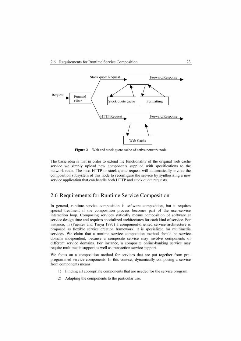
2.6 Requirements for Runtime Service Composition 23
Forward/Response
Request Protocol Filter FormattingStock quote cache
Forward/Response Stock quote Request
Web Cache
HTTP Request
Figure 2 Web and stock quote cache of active network node
The basic idea is that in order to extend the functionality of the original web cache service we simply upload new components supplied with specifications to the network node. The next HTTP or stock quote request will automatically invoke the composition subsystem of this node to reconfigure the service by synthesizing a new service application that can handle both HTTP and stock quote requests.
2.6 Requirements for Runtime Service Composition
In general, runtime service composition is software composition, but it requires special treatment if the composition process becomes part of the user-service interaction loop. Composing services statically means composition of software at service design time and requires specialized architectures for each kind of service. For instance, in (Fuentes and Troya 1997) a component-oriented service architecture is proposed as flexible service creation framework. It is specialized for multimedia services. We claim that a runtime service composition method should be service domain independent, because a composite service may involve components of different service domains. For instance, a composite online-banking service may require multimedia support as well as transaction service support.
We focus on a composition method for services that are put together from pre-programmed service components. In this context, dynamically composing a service from components means:
1) Finding all appropriate components that are needed for the service program.
2) Adapting the components to the particular use.

Chapter 2 Services and Runtime Service Composition 24
3) Synthesizing the interface code that matches the components to the context of their use.
A service is composed on the basis of a service request that specifies the service. For instance, the service to withdraw funds from a bank has the following request:
“Given bank, account and amount that has to be withdrawn, build a service program that receives a bank identifier, an account number, and amount as input and returns funds.”
Composing a service on request puts hard requirements on the composition method:
1) The composition method must be efficient, because the composition is performed in a dynamic service environment (in the user interaction loop).
2) The composition method must work autonomously, because the user has no abilities to provide help in the synthesis process.
3) The composition method must guarantee correct deployment of components.
4) Even more importantly, the composition method must also provide a specification language that enables one to specify services and components in a reasonably easy way.
We define a runtime composite service as a service where the actual service program is composed on service request. Hence, the first requirement, the efficiency of the composition method, results from the additional step (i.e. the actual service composition) that must be taken in a dynamic service environment. The service response time in traditional service environments depends on resource latencies (network, database, etc.), server load, and service execution time. In our case the service response time includes additionally the service composition time. Therefore the composition method must be time-efficient in order to provide a service composition with low costs.
In dynamic service composition environments it is not acceptable to involve end users in service composition. Hence, there is no user-service interaction during the service composition process. That gives us the second requirement of the composition method: the composition method must proceed autonomously.
The third requirement, the guarantee of correct deployment of components, is obvious. This requirement can be satisfied by the logical correctness of the composition method and by correctness of specifications of components. In this thesis we propose a logic and a specification language that enable us to reason about and to deploy service components automatically. The proposed composition method uses a logical proof as witness for the correct usage of service components.
A key requirement to our composition method is to provide a specification logic that enables us to reason automatically about service components. The specification logic allows us to find automatically all appropriate service components that are needed for a service to be composed and to synthesize the interface code that matches the service

2.6 Requirements for Runtime Service Composition 25
components (calls methods of classes). An essential feature of our proposed logic is the possibility to express dependencies of service components from different sources. This enables us to specify service component capabilities and the context where a service component can be used during application composition.


Chap t e r 3
A Calculus for Runtime Service Composition
In this chapter, we present the core of our approach to runtime service composition. We study the calculus of the Structural Synthesis of Programs (SSP), which we have extended according to the needs of service composition. We call this extension the Extended Structural Synthesis of Programs (ESSP). The SSP, as put forth by Tyugu and Mints (Mints and Tyugu 1982), is a deductive approach to the synthesis of programs from specifications. The logical language employed in SSP uses the logical conjunction and implication connectives only, i.e., it is an implicative fragment of intuitionistic propositional calculus. In contrast, the logic employed in ESSP is a fragment of intuitionistic first-order calculus. ESSP embodies theoretical developments stemming from SSP.
The ESSP makes three extensions to the SSP. First, it introduces disjunction into the logical language, second, it adds falsity to the logical language, and third, it introduces quantifiers in a restricted way in order to keep proof search manageable, i.e., efficient. These extensions are justified by the following three observations:
Alternative outcome of modules. In services we often meet a situation where a module (function, method, procedure) may produce one of several alternative outputs every time it is applied. In particular, this is the case with exception handling – we expect that a normal output will be produced, but
27

Chapter 3 A Calculus for Runtime Service Composition 28
must be ready to handle exceptions when they appear. This requires introduction of disjunctions on the right-hand side of implications.
Program termination after exception handling. Modules may throw exceptions. At specification time we often do not know in advance how computation should continue after exception handling. This requires falsity on the right-hand side of implications.
Implicit selection and linking of software components. Our intention is to use the synthesizer to put together large service programs from components. By a component we mean not just a function, but also a software configuration providing some useful functionality. We expect to have libraries of components supporting various problem domains, like packages in Java. So, the problem of automatic selection of components appears. This requires a language where we can state that a component with particular properties exists or, vice versa, may be required. Hence, we need existential and universal quantifiers. However, we can restrict the usage of quantifiers so that we will not need the full expressive power of first-order logic.
We present the structural synthesis of programs in section 3.2. Then we describe the extended structural synthesis of programs in section 3.3. However, we start with a short introduction to natural deduction and intuitionistic logic, the logic employed by our calculus for runtime service composition.
3.1 Preliminaries
3.1.1 Intuitionistic Logic Intuitionistic logic can succinctly be described as classical logic without the Aristotelian law of excluded middle (A∨¬A), but with the law of contradiction (¬A⊃(A⊃B)). Its logical operations ∧, ∨, ⊃ (intuitionistic implication), ∀, ∃ are constructively independent, i.e., formulae equivalent in the classical situation can become different in the intuitionistic case. For example, classically (A∨B) is equivalent to ¬(¬A ∧ ¬B), and ∃xA(x) is equivalent to ¬∀x¬A(x). Intuitionistically, a sentence of the form (A∨B) asserts that either a proof of A or a proof of B has been constructed while ¬(¬A ∧ ¬B) asserts that an algorithm has been constructed which would effectively convert any pair of constructions proving ¬A and ¬B respectively, into a proof of a known contradiction. Hence, the two sentences are different. Gödel interpreted the results in (Gödel 1933) as showing that intuitionistic logic is richer than classical logic, because intuitionistic logic distinguishes formulae that are classically equivalent. A formal system for classical first-order predicate logic can be obtained by replacing the law of contradiction with the double negation law ¬¬A⊃A or, equivalently, by the law of excluded middle (A∨¬A). A system of classical natural

3.1 Preliminaries 29
deduction can be constructed by adding one additional rule of inference, which are the proof by contradiction rule ( ), the double negation elimination rule (u
C⊥ C¬¬ ), or the rule of excluded middle ( XM ).
uC
uA
A
¬
⊥⊥
CA
A¬¬
¬¬ XMA A∨ ¬
The computational interpretation of the logical connectives in intuitionistic logic makes intuitionistic logic a suitable logic for our needs. The SSP, for instance, uses a fragment of intuitionistic propositional logic that renders a feasible balance between the expressiveness of the logical language and the efficiency of synthesis (Uustalu 1995c). In SSP, programs are constructed from pre-programmed modules (first-order and second-order functions) taking into account only structural properties of programs being synthesized. This fact relates the idea of program construction of SSP directly to intuitionistic propositional logic in the following sense: input and output domains of existing modules can be represented by propositional variables. The implication connective is interpreted as computational step. That is as the execution of a module. The conjunction connective specifies composition of objects into a structure.
Intuitionistic logic is a constructive logic. Constructive logics have the valuable property that any proof of existence of an object contains complete information for constructing (i.e., computing) the object. In particular, formulae of intuitionistic logic (which is the most commonly used constructive logic) have this information in the realizations (i.e., proof terms, see section 3.1.3.4) associated with them. We assume that the realization of every axiom is given. The realization of a formula derived by means of an inference rule of an intuitionistic calculus is constructed from the realizations of premises of the rule. In this way, every derivable formula of intuitionistic logic receives a realization.
3.1.2 Natural Deduction The core of our proposed method to service composition is a calculus that allows us to compose service programs efficiently. It is a fragment of the calculus of intuitionistic natural deduction. In this section we briefly introduce the calculus of natural deduction due to Gentzen (Gentzen 1969). We summarize properties and relate intuitionistic natural deduction to programs.
The fundamental notion is that of a judgment based on evidence. For example, we might make the judgment "The sun is shining" based on visual evidence. There are certain forms of judgments, which have been investigated. We will use only hypothetical judgments.

Chapter 3 A Calculus for Runtime Service Composition 30
A hypothetical judgment has the form "J2 under hypothesis J1" and is interpreted as follows: provided with evidence for J1 we can make the judgment J2. Formal evidence for a hypothetical judgment is a hypothetical derivation. Here, the hypothesis J1 can be freely used in the derivation of J2. Hypotheses need not to be used, and could be used more than once.
The formal evidence for a judgment in form of a derivation is usually written in a two-dimensional notation:
JD
if D is a derivation of J. A hypothetical judgment is written as
2
1
J
uJ
where u is a label which identifies the hypothesis J1. Labels are used to guarantee that hypotheses, which are introduced during the reasoning process, are not used outside their scope. Operationally, if we relate this to programs, it means that we restrict the use of local objects of a branch of a program to that branch only, i.e., objects occurring within a branch of a program cannot be used within any other branch of the same program.
There are two important properties of Gentzen's system of natural deduction, which are often mentioned in literature. One is that we can define all logical connectives without reference to any other connective. This simplifies the consideration of fragments and extension of logics. That is important for us since we use a logic that is a fragment of intuitionistic propositional logic. The other important property of natural deduction systems is that its proofs are isomorphic to the terms in the λ-calculus via the so-called Curry-Howard isomorphism (Howard 1980). This isomorphism establishes many connections to functional programming and is in literature often called the propositions-as-types or proofs-as-programs paradigm.
3.1.3 Intuitionistic Natural Deduction We use a fragment of intuitionistic logic. Therefore, we briefly describe natural deduction for this logic. Valid deductions are described through inference rules, which at the same time explain the meaning of the logical connectives in terms of their proof rules.
The language of propositions is built up in the usual way from proposition symbols A, B, etc. and the logical connectives.
Propositions A ::= A1 ∧ A2 | A1 ⊃ A2 | A1 ∨ A2 | ¬A | 2 | 3 | ∀x.A | ∃x.A

3.1 Preliminaries 31
A propositional constant A is simply a predicate symbol without arguments; it is written A instead of A(). The meaning of a propositional symbol is left unspecified here and only made concrete for specific theories. For instance, the proposition X may have the meaning “variable x has a correct value”.
We use parentheses to disambiguate and assume that ∧ and ∨ bind stronger than ⊃. The main judgment of intuitionistic natural deduction is "A is true", written as 0 A. It is derived from the hypotheses 0 A1,…, 0 An, which makes it a hypothetical judgment.
In natural deduction logical connectives are characterized by their introduction and elimination rules. An introduction rule specifies how to infer that a compound sentence (e.g., conjunction) is true from the truth of its constituent parts, while an elimination rule specifies what other truths can be deduced from the truth of compound sentences. The local soundness and local completeness properties guarantee that if introduction and elimination rules match, then they are meaningful. The logical constant 2 (Truth), however, has only an introduction rule while 3 (falsehood) has only an elimination rule. The local soundness property guarantees that if we introduce a connective and immediately eliminate it again, we should be able to remove the introduction and elimination and obtain a shorter derivation without using the connective. If we can conclude more than we should be able to, then the elimination rule is too strong. The local completeness property assures that an elimination of a connective retains sufficient information so that we can reconstruct the eliminated connective immediately by an introduction rule. Local soundness and completeness of inference rules can be proved by means of local reduction and expansion.
Independently from any derivation, certain structural properties of derivations are assumed. These are: hypothesis, i.e., if we have a hypothesis 0 A than we can conclude 0 A; weakening, i.e., hypotheses need not be used; duplication, i.e., hypotheses can be used more than once; exchange, i.e., the order in which hypotheses are introduced is irrelevant.
An important principle of natural deduction is that each logical connective is defined in terms of inference rules without referring to other connectives, which is called orthogonality of connectives.
3.1.3.1 Inference Rules We briefly comment only on three pairs of inference rules, for conjunction, implication, and negation. A more detailed discussion on inference rules of natural deduction systems (which we present in Table 1) can be found in (Prawitz 1965). In the following, the symbol ⇒ denotes a transformation between two derivations, where ⇒R denotes a reduction and ⇒E denotes an expansion. Reduction is used to prove local soundness and expansion is used to prove local completeness. The reduction and expansion transformations relate derivations with the same conclusion.

Chapter 3 A Calculus for Runtime Service Composition 32
A conjunction A ∧ B is true if A and B are true. Hence, the introduction rule is as follows:
IA BA B
∧∧
0 00
If we know A ∧ B we should be able to reestablish the truth of A and B and thus have two elimination rules.
LEA BA∧ ∧0
0 REA B
B∧ ∧0
0
To check whether our rules for conjunction are locally sound, we consider the following two reductions between derivations. The derivations to be reduced end in an introduction followed by an elimination.
1 2
L
IE
R
D DA B
A BA
⇒∧∧ ∧0 0
00
1DA0
1 2
R
IE
R
D DA B
A BB
⇒∧∧ ∧0 0
00
2DB0
To show that the rules a locally complete, we reintroduce a conjunction from its components in the form of a local expansion.
DA B∧0
E⇒ L RE EI
D DA B A B
A BA B
∧ ∧∧ ∧∧
∧
0 00 0
0
Similarly, to derive an implication 0 A ⊃ B we assume 0 A and then derive 0 B, which is written as hypothetical judgment:
Iu
uA
BA B
⊃⊃
0
00
It is very important that we ensure that the hypothesis 0 A is available only in the derivation above the premise, which is indicated by the labeled inference. The label is the hypothesis u, which must not already be used as the name for a hypothesis in the derivation of the premise. The identifier ⊃ Iu means that the hypothesis 0 A labeled with u is discharged at the inference labeled with ⊃ Iu. Hence, a derivation of 0 A ⊃ B describes a construction by which a derivation of 0 A is transformed into a derivation of 0 B. The elimination rules describes how we can obtain a derivation of 0 B if we have derivations of 0 A ⊃ B and 0 A.

3.1 Preliminaries 33
EA B AB
⊃ ⊃0 00
The local reduction rule performs a substitution through which the derivation of 0 A is substituted wherever the assumption 0 A is used in the hypothetical derivation of 0 B.
12
IE
u
uAD
DBA B
BA
⊃⊃
⊃
0
00
00
R⇒
2
1
D uAD
B
0
0
An implication can again be rebuilt by local expansion.
DA B⊃0
E⇒ EIu
Du
A B AB
A B
⊃ ⊃⊃
⊃
0 00
0
In order to derive ¬A we assume A and try to derive a contradiction. This requires falsehood, i.e., we consider ¬A as an abbreviation of A ⊃ ⊥. The negation introduction rules employs a judgment that is parametric in a propositional parameter p: if we can derive any p from the hypothesis A we conclude ¬A. The negation elimination rule can be viewed as a combination of implication elimination and falsehood elimination (see Table 1) if we consider ¬A as an abbreviation for A ⊃ ⊥. Hence, if we can derive falsehood, we can derive everything. The local reduction is the following:
12,I
E
p u
uAD
DpA
CA
¬¬
¬
0
00
00
R⇒
2
1/
D uAC p D
C
0
0
The substitution is valid, since D1 is parametric in p. The local expansion is similar to the case for implication.
1/C p D
DA¬0
E⇒ ,
EI p u
Du
A ApA
¬
¬
¬¬
0 00
0

Chapter 3 A Calculus for Runtime Service Composition 34
In the elimination and introduction rules for universal and existential quantification we use a for any parameter about which we can make no assumptions and we use t for any term. We say that .x A∀
. is provable if [a/x]A is provable for a new parameter a.
Conversely, if we know x A∀ , we know that [t/x]A for any term t. We conclude that .x A∃ is true when there is a term t such that [t/x]A is true. When we have an
assumption .x A∃ we do not know for which term t it is the case that [t/x]A holds. We can only assume that [a/x]A holds for some fresh parameter a about which we know nothing else.

3.1 Preliminaries 35
Table 1 Inference rules of intuitionistic propositional natural deduction
Introduction Rules Elimination Rules
IA BA B
∧∧
0 00
LEA BA∧ ∧0
0 REA BB∧ ∧0
0
LIAA B
∨∨
00 RIB
A B∨
∨0
0
, Eu w
u wA B
A B C CC
∨ ∨
0 0
0 0 00
Iu
uA
BA B
⊃⊃
0
00
EA B AB
⊃ ⊃0 00
,I p u
uA
pA
¬¬
0
00
EA AC
¬ ¬0 00
I20 2
no 2 elimination
no 3 introduction EC
00
3 3
[ / ] I.
aa x Ax A
∀∀
00
2 . E[ / ]
x At x A∀
∀0
0
[ / ] I.
t x Ax A
∃∃
00
,
[ / ]
. Ea u
ua x A
x A CC
∃ ∃
0
0 00
3
2 a must be new, it must not occur in any undischarged assumption in the proof of [a/x]A or in .x A∀ itself. 3 a must be new, it must not occur in .x A∃ , C or any assumption used in the derivation of the second
premise.

Chapter 3 A Calculus for Runtime Service Composition 36
3.1.3.2 Localizing Hypotheses The correct usage of hypothesis is a global property of a derivation. In order to make available hypotheses explicitly visible at each derivation step we annotate each judgment in a derivation by the available hypotheses, i.e., we localize hypotheses. Hypotheses are notated in a context.
:: | , :Contexts u AΓ = ⋅ Γ
Here, “⋅” represents the empty context, and Γ, u:A adds hypothesis 0 A labeled with u to Γ. Each label occurs at most once in a context. The main judgment is now written Γ 0 A, where ⋅, u1:A1, …, un:An 0 A stands for
1 n1 n
u uA A
A
0 0
0.
The empty context can be omitted and contexts can be concatenated as follows: Γ, ⋅ = Γ Γ,(Γ’, u:A) = (Γ, Γ’), u:A.
In addition we add the following hypothesis rule, which was implicit before.
1 2, : ,u
u A AΓ Γ 0
The localized versions of inference rules are shown in Table 2.

3.1 Preliminaries 37
Table 2 Localized version of inference rules
Introduction Rules Elimination Rules
IA BA B
Γ ΓΓ
∧∧
0 00
LEA BA
ΓΓ
∧ ∧00 REA B
BΓ
Γ∧ ∧0
0
LIA
A BΓ
Γ∨
∨0
0 RIBA B
ΓΓ
∨∨
00
, , : , : Eu wA B u A C w B CC
Γ Γ ΓΓ
∨ ∨0 0 00
, : Iuu A BA B
ΓΓ
⊃⊃0
0 EA B A
BΓ Γ
Γ⊃ ⊃0 0
0
,, : I p uu A pA
ΓΓ
¬¬
00
EA AC
Γ ΓΓ
¬ ¬0 00
IΓ
20 2
no 2 elimination
no 3 introduction EC
ΓΓ
00
3 3
[ / ] I.
aa x Ax A
Γ∀
Γ ∀00
. E[ / ]
x At x A
Γ ∀∀
Γ0
0
[ / ] I.
t x Ax A
Γ∃
Γ ∃00
,. , :[ / ] Ea ux A u a x A CC
Γ ∃ Γ∃
Γ0 0
0
3.1.3.3 Structural Properties of Hypothesis The following properties hold for intuitionistic natural deduction.
Exchange: 1 1 2 2 3 1 2 2 1 3, : , , : , , : , , : ,If u A u B C then u B u A CΓ Γ Γ Γ Γ Γ0 0
Weakening: 1 2 1 2, , : ,If C then u A CΓ Γ Γ Γ0 0
Contraction: 1 1 2 2 3 1 2 3, : , , : , , : , ,If u A u A C then u A CΓ Γ Γ Γ Γ Γ0 0
Substitution: 1 2 1 1 2, : , ,If u A C and A then CΓ Γ Γ Γ Γ0 0 0
The proof of these properties is by structural induction over derivations. The proof can be found in (Prawitz 1965).

Chapter 3 A Calculus for Runtime Service Composition 38
3.1.3.4 Proof Terms Proof terms are used to localize the derivations themselves. Howard (Howard 1980) has noted that there is a correspondence between intuitionistic derivations and λ-terms. Formulas act as types classifying λ-terms. The analogy between propositions and types is also discussed in (Coquand 1986). This correspondence is an isomorphism for the propositional case: formulae are isomorphic to types and derivations are isomorphic to simply-typed λ-terms. In the literature this isomorphism is often called the propositions-as-types or proofs-as-programs paradigm.
In general, to express that the judgment “M is a proof term for the proposition A under hypotheses Γ” holds, we write Γ 0 M : A. Formal evidence for this judgment is given in form of the derivation of M : A from Γ. We can view proof terms as the justification of formulae: we are no longer satisfied with demonstrating the truth of a formula but demonstrate at the same time the reason (in the form of a proof term) for which the formula is true (Coquand 1986). The proof term M of the proposition A is also called its witness.
For brevity, we introduce only proof terms for conjunction, implication, and negation. We do not discuss local reduction and expansion of proof terms. A detailed description on proof terms can be found in (Prawitz 1965). We summarize the inference rules for localizing derivations using proof terms in Table 3.
The proof term for a conjunction introduction is the pair of proofs of the premises. If M represents a proof of A and N represents a proof of B, then the pair ⟨M, N⟩ represents the proof of A∧B by conjunction introduction.
: : I, :
M A N BM N A B
Γ ΓΓ
∧∧
0 00
Similarly for the conjunction elimination rules, if M represents a proof of A∧B, then fst M extracts the proof term of A from M, and snd M represents the proof term of B.
L: E
fst :M A B
M AΓΓ
∧ ∧00 R
: Esnd :M A B
M BΓΓ
∧ ∧00
The proof of an implication A⊃B represents a function that maps proofs of A to proofs of B. The introduction rule creates such function by λ-abstraction.
, : : I( : . ) :
uu A M Bu A M A Bλ
Γ ⊃⊃
00
The elimination rule represents the application of the function corresponding to M to an argument N of type A.
: : E:
M A B N AM N B
Γ ΓΓ
⊃ ⊃0 00

3.1 Preliminaries 39
In the conclusion of the implication introduction rule the variable u is bound. This signals that the hypothesis is discharged and not available outside of the deduction of the premise.
Negation is similar to implication. Since the premise of the rule is parametric in p the corresponding proof constructor must bind a propositional variable p, indicated by µp.
,, : : I: . :
p upu A M pu A M Aµ
Γ ¬¬
0
0
Similarly, the elimination construct must record the formula C to maintain the property that every valid term proves exactly one proposition. This is indicated as a subscript C to the infix operator “⋅”.
: : E:C
M A N AM N C
Γ ΓΓ ⋅¬ ¬0 0
0
The following table shows all inference rules using proof terms.

Chapter 3 A Calculus for Runtime Service Composition 40
Table 3 Inference rules using proof terms
Introduction Rules Elimination Rules
: : I, :
M A N BM N A B
Γ ΓΓ
∧∧
0 00
L: E
fst :M A B
M AΓΓ
∧ ∧00
R: E
snd :M A B
M BΓΓ
∧ ∧00
L: I
inl :BM AM A B
Γ
Γ∨
∨0
0
R: I
inr :AN BN A B
Γ
Γ∨
∨0
0
, 1 2
1 2
: , : : , : : E(case of inl | inr ) :
u wB A
M A B u A N C w B N CM u N w N C
Γ Γ Γ
Γ ⇒ ⇒
∨ ∨0 0 0
0
, : : I( : . ) :
uu A M Bu A M A Bλ
Γ ⊃⊃
00
: : E:
M A B N AM N B
Γ ΓΓ⊃ ⊃0 00
,, : : I: . :
p upu A M pu A M Aµ
Γ ¬¬
0
0 : : E
:C
M A N AM N C
Γ ΓΓ ⋅¬ ¬0 0
0
I:Γ
20 2
no 2 elimination
no 3 introduction : E
abort :CM
M CΓ
Γ
0
0
3 3
[ / ] :[ / ] I. : .
aa x M a x Ax M x Aλ
Γ∀
Γ ∀0
0 : . E
:[ / ]M x A
Mt t x AΓ ∀
∀Γ
00
:[ / ] I, : .
M t x At M x A
Γ∃
Γ ∃0
0 ,: . , :[ / ] [ / ] : E
let , in :a uM x A u a x A a x N C
x u M N CΓ ∃ Γ
∃Γ =
0 00
3.1.4 Derivation Example and Program Extraction from Proofs As an example consider the formula F
( ) (( ) ) (( ) )X Y Z Y Z J X J I I∧ ⊃ ∧ ⊃ ⊃ ∧ ⊃ ⊃ ⊃ ,
which should be derivable. Let H, G, and F be abbreviations for sub-formulae as follows:
( )( )
H X JG Y Z JF X Y Z
I≡ ⊃ ⊃≡ ⊃ ⊃≡ ∧ ⊃
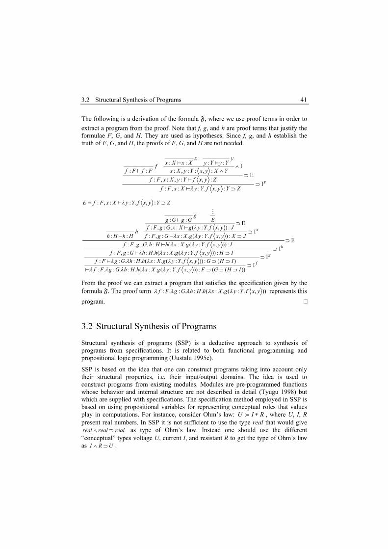
3.2 Structural Synthesis of Programs 41
The following is a derivation of the formula F, where we use proof terms in order to extract a program from the proof. Note that f, g, and h are proof terms that justify the formulae F, G, and H. They are used as hypotheses. Since f, g, and h establish the truth of F, G, and H, the proofs of F, G, and H are not needed.
: : : : I: : : , : : , :
E: , : , : , :
I: , : : . , :
y
x yx X x X y Y y Yf
f F f F x X y Y x y X Yf F x X y Y f x y Z
f F x X y Y f x y Y Zλ
∧∧
⊃⊃
⊃
0 00
0
0
: , : : . , :
: : E: , : , : ( : . , ) :
I: : : , : : . ( : . , ) :
: , : , : ( : . ( : . , )) :: , : : . ( : . ( : . , )) :
: : . : . ( : . ( : .
x
E f F x X y Y f x y Y Z
gg G g G E
f F g G x X g y Y f x y Jh
h H h H f F g G x X g y Y f x y X Jf F g G h H h x X g y Y f x y I
f F g G h H h x X g y Y f x y H If F g G h H h x X g y Y
λ
λλ λ
λ λλ λ λ
λ λ λ λ
≡ ⊃
⊃⊃
⊃
⊃
0
00
0 00
00
EI
I, )) : ( )
I: . : . : . ( : . ( : . , )) : ( ( ))
h
g
ff x y G H If F g G h H h x X g y Y f x y F G H Iλ λ λ λ λ
⊃⊃
⊃⊃ ⊃
⊃⊃ ⊃ ⊃0
From the proof we can extract a program that satisfies the specification given by the formula F. The proof term : . : . : . ( : . ( : . , ))f F g G h H h x X g y Y f x yλ λ λ λ λ represents this program.
3.2 Structural Synthesis of Programs
Structural synthesis of programs (SSP) is a deductive approach to synthesis of programs from specifications. It is related to both functional programming and propositional logic programming (Uustalu 1995c).
SSP is based on the idea that one can construct programs taking into account only their structural properties, i.e. their input/output domains. The idea is used to construct programs from existing modules. Modules are pre-programmed functions whose behavior and internal structure are not described in detail (Tyugu 1998) but which are supplied with specifications. The specification method employed in SSP is based on using propositional variables for representing conceptual roles that values play in computations. For instance, consider Ohm’s law: U RI ∗=: , where U, I, R present real numbers. In SSP it is not sufficient to use the type real that would give
as type of Ohm’s law. Instead one should use the different “conceptual” types voltage U, current I, and resistant R to get the type of Ohm’s law as .
real real real∧ ⊃
I R U∧ ⊃

Chapter 3 A Calculus for Runtime Service Composition 42
The language of SSP consists of intuitionistic propositional formulae. A synthesis problem is represented as a sequent Г 0 G, where Г is a list of formulae. The formulae of Г are called the premises of the synthesis problem and specify the pre-programmed modules, while the formula G is called the goal of the synthesis problem and specifies the program to be synthesized. Any propositional variable here expresses the fact that a value of its corresponding object variable can be computed. In other words, this computation becomes the realization of the propositional variable.
In order to specify pre-programmed functions of synthesized programs more precisely than the SSP language permits, one should use a richer language for annotating axioms. These annotations can be used both for verification of synthesized programs and for guidance of the proof-search in order to avoid incorrect solutions. Tammet has proven correctness of some set manipulation programs using first-order annotations of axioms of SSP (Tammet 1999).
The two facts (i) using propositional variables as identifiers for conceptual roles in the specification method and (ii) using intuitionistic propositional logic for solving synthesis problems are fundamental for the synthesis method employed in SSP. The synthesis method is based on the proofs-as-programs property of intuitionistic logic. This equates the problem of program synthesis to the problem of proof search (Mints and Tyugu 1982).
Structural synthesis of programs has been known for a number of years. It has been used in two commercial systems, XpertPriz and Priz (Tyugu 1991b). SSP is also the basis for programming in the NUT system (Uustalu et al. 1994). Applications of the SSP are presented in (Tyugu, Matskin, and Penjam 1999). All programming environments that support SSP work in the implicative fragment of intuitionistic propositional logic. Intuitionistic propositional logic renders a feasible balance between the expressiveness of the specification language and the efficiency of synthesis (Uustalu 1995c).
3.2.1 Logical Language LL In SSP a specification of a pre-programmed module is used as an axiom stating under which conditions the module can be applied and which values it computes. The relation between the individual input and output values is not described in the axiom. Therefore, the general form of a program module specification (Manna and Waldinger 1993)
.( ( ) . ( , ))x P x y R x y∀ ⊃ ∃
with precondition P and postcondition R is replaced in SSP by
.( ( ) . ( ))x P x y R y∀ ⊃ ∃ .

3.2 Structural Synthesis of Programs 43
The meaning of this specification is that a correct value (satisfying R) can be computed from a correct input (satisfying P). The relation between input and output values is not given, because SSP relies on the pre-programmed module that is supposed to compute a correct value. The equivalent of the latter formula is
. ( ) . ( )x P x y R y∃ ⊃ ∃ .
The closed formulae ∃ and )(. xPx )(. yRy∃ can be considered as propositions where the internal structure of those propositions is inessential. Thus, axioms can be presented in a propositional language (Tyugu 1998) as follows:
. ( ) . ( )x P x y R y∃ ⊃ ∃
⊃P RP R
In SSP it is assumed that some programming language outside the logic provides realizations of the axioms (i.e., pre-programmed modules).
The logical language of SSP, which is called LL, allows three kinds of formulae. This restriction on the form of formulae does not lead to any loss in the expressiveness of the logical language, as we will see later in section 3.2.3. The allowed formulae are 1) propositional variables, 2) unconditional computability statements, and 3) conditional computability statements. The general form of a formula is:
( )1 1 1
iij i k
nn mU V X
i j kY⊃ ∧ ⊃
= = =∧ ∧ ∧
where n, m≥0, ni≥1 and the Uij’s, Vi’s, Xk’s, and Y are propositional variables. Any part on the left-hand side of the main implication may be empty. An empty conjunction is identified with 2, and formulae of the form Y⊃2 are identified with Y, which represents the first kind of formulae, a propositional variable. For n = 0 we get an unconditional computability statement (i.e., simple implication), and for n > 0 we get a conditional computability statement (i.e., nested implication). We use X as
abbreviation for 1
k
mX
k =∧ and (U V )⊃ as abbreviation for . ( )
1 1
iij iU V⊃
nn
i j= =∧ ∧
The computational meaning of LL-formulae can succinctly be described as follows:
Propositional variables of LL correspond to object variables. For example, if we have an object variable y occurring in some specification then there is a propositional variable Y in the logical language that expresses computability of a value of the object variable y.

Chapter 3 A Calculus for Runtime Service Composition 44
An unconditional computability statement X Y⊃ expresses computability of the value of the object variable y corresponding to Y from values of x1, …, xm corresponding to X.
A conditional computability statement ( )U V X Y⊃ ∧ ⊃ expresses the computability of the value of the object variable y from the value of x depending on the computations of the values of the object variables vi’s from the uij’s.
The realization of an axiom of the form ( )U V X Y⊃ ∧ ⊃ can be an arbitrarily complex module that calls synthesized realizations of subgoals ( )U V⊃ , which we call subtasks. Subtasks can be called in any suitable order and as many times as needed. This provides generality to the structural synthesis of programs: any kind of usage of subtasks can be pre-programmed.
3.2.2 Inference Rules As already mentioned above, the SSP uses intuitionistic logic, which guarantees constructiveness of proofs. The logical language LL allows formulae only containing the implication and conjunction connectives. Therefore, it is sufficient to use introduction and elimination rules for implication and conjunction. As usual in logic, inference rules are used for constructing a proof (i.e., a derivation tree) of a formula. Leaves in a derivation tree represent axioms and other nodes represent inference steps, where one of the inference rules is applied and a new formula is derived (Uustalu 1995a).
The localized version of natural deduction rules for handling implications and conjunction are the same as presented in chapter 3.1.3.2.
Table 4 Conventional inference rules (SSP)
Introduction Rules Elimination Rules
IA BA B
Γ ΓΓ
∧∧
0 00
LEA BA
ΓΓ
∧ ∧00
REA BB
ΓΓ
∧ ∧00
, : Iuu A BA B
ΓΓ
⊃⊃0
0 EA B A
BΓ Γ
Γ⊃ ⊃0 0
0
Note that introduction and elimination rules with two premises (∧I, ⊃E) given in Table 4 make use of the structural properties of hypothesis discussed in section 3.1.3.3.

3.2 Structural Synthesis of Programs 45
3.2.3 Completeness of LL The restriction on the form of formulae does not lead to a loss of logical expressiveness of the language. Any given propositional formula F among the premises of a sequent can be efficiently transformed into a deductively equivalent set SF of formulae of the form of LL. This transformation uses the equivalence replacement theorem ( ) ( [F ])X F G G X⇔ ⇒ ⇔ , where G is the result of substitution of X for F in G
[ ]F X
(Mints and Tyugu 1982), ⇔ denotes logical equivalence and ⇒ denotes logical implication. We can substitute new variables for sub-formulae, and reduce the depth of a formula as well as eliminate disjunction, equivalence and negation connectives in it, transforming the formula into the form of LL.
A sub-formula A ⊛ B (where ⊛ is one of the logical connectives: ∧, ∨, ⊃) of F is replaced by introducing a new propositional variable X. The transformation rules are as follows:
A ⊛ B Add to SF
A ∧ B X ⊃ A, X ⊃ B, A ∧ B ⊃ X
A ∨ B X ⊃ A ∨ B, A ⊃ X, B ⊃ X
A ⊃ B X ∧ A ⊃ B, (A ⊃ B) ⊃ X
In order to eliminate occurrences of disjunction and negation in SF, two additional transformation rules are needed.
Elimination of disjunction. The transformation rule for elimination of disjunction is as follows: a formula X A B⊃ ∨
( ) occurring in SF is replaced with the set of formulae
( )X A p∧ ⊃ B p p∧ ⊃ ⊃ for all propositional variables p of the theory. This is justified by the second order equivalence ( ) (( ) ( )a b p a p b p p∨ ⇔ ∀ ⊃ ∧ ⊃ ⊃ )
Elimination of negation. Formulae of the form ¬A are (equivalently) expressed as A ⊃⊥ , where ⊥ is the falsity constant. The new variable L and the formula L K Z⇔ ∧ where Z is a new variable and K is the conjunction of all propositional variables of the theory can replace the falsity constant. This is justified by the second order equivalence xx⊥⇔ ∀ .
Example. Consider the following formula (( ) )F P Q V V≡ ⊃ ⊃ ⊃ , which is not a formula of the logical language of SSP. The formula F is transformed into its deductively equivalent set of formulae SF as follows. Let X represent the sub-formula
of F, then, the set of formulae SF is {P Q⊃ X P Q∧ ⊃ ( )P Q, X⊃ ⊃ }. The whole set of formulae is { ( )X V V⊃ ⊃ } ∪ SF.

Chapter 3 A Calculus for Runtime Service Composition 46
3.2.4 Program Extraction Each formula of the logical language LL has a computational meaning. We use Kleene realizability of intuitionistic formulae, and associate a proof term (i.e., program or pre-programmed module) with each derivable formula (Matskin and Tyugu 1999).
The logical language LL extended with terms is as follows.
1) A propositional variable corresponds to an object variable: a , where A is a propositional variable and a is the corresponding object.
A:
2) An unconditional computability statement has a computational interpretation as a function f for computing b from ai’s, i.e. ai’s are inputs and b is the output of f.
1 n1
... . :n
ii
a a f A Bλ=
⊃∧
3) A conditional computability statement denotes the computability of y depending on xj’s and on the computation of all vi’s from uij’s.
1 11 1 1
... ... . : ( )inn m
n m ij i ji j j
g g x x f U V X Yλ= = =
⊃ ∧ ⊃∧ ∧ ∧
where gi, i = 1, …, n, are functional variables denoting realizations ei of subtasks that should be synthesized:
11
... . : ( )i
i
n
i in i ij ij
u u e U Vλ=
⊃∧
In order to extract programs from constructive proofs we need to extend the inference rules according to the language LL extended with terms. The inference rules supplied with proof terms for conjunction introduction and elimination as well as implication introduction and elimination are the same as presented in section 3.1.3.4.
Table 5 Conventional inference rules using proof terms (SSP)
Introduction Rules Elimination Rules
: : I, :
M A N BM N A B
Γ ΓΓ
∧∧
0 00
L: E
fst :M A B
M AΓΓ
∧ ∧00
R: E
snd :M A B
M BΓΓ
∧ ∧00
, : : I( : . ) :
uu A M Bu A M A Bλ
Γ ⊃⊃
00
: : E:
M A B N AM N B
Γ ΓΓ⊃ ⊃0 00

3.2 Structural Synthesis of Programs 47
Program extraction occurs at each inference step. Realizations of the axioms are given. The realization of an assumption X is an object variable x. Realization of a derived formula is built step by step from realizations of premises of applied inference rules according to Table 5.
Due to the use of the conventional inference rules of the intuitionistic propositional calculus, extracted programs will contain unnecessary steps of composition and decomposition of data structures that correspond to realizations of conjunctions appearing in a derivation. This fact makes the conventional inference rules unsuitable for program synthesis, because they may lead to inefficient programs. The SSP therefore uses so-called structural synthesis rules (SSR) to overcome this shortcoming. We briefly describe these rules in the next section.
3.2.5 Structural Synthesis Rules The main strategy of the SSP is based on the idea to use computability information present in the axioms to direct the search. Instead of using the conventional rules of the intuitionistic propositional calculus, admissible rules are used. Every application of an admissible elimination rule corresponds exactly to an application of a pre-programmed module represented by an axiom, i.e., corresponds to a computational step performed by calling a program that is the realization of the axiom (Matskin and Tyugu 1999, Matskin and Tyugu 2001).
The inference rules of the SSP can be represented using a sequent notation. Consider the sequent XΓ0 , where Г is a list of formulae and X is a formula. We will also use another representation of specifications where a sequent 0 is an axiom. These axioms are called specific or problem-oriented axioms, because they express the specific knowledge about particular problems. Axioms have the following form:
F
, A AΓ 0 and 0 , where F is an axiom of the theory. F
Admissible inference rules employed by the SSP are presented below. These rules are also known as structural synthesis rules (SSR).
Implication Introduction
, : Iuu A BA B
ΓΓ
⊃⊃0
0
where :u A is a conjunction of formulae. The introduction rule remains the same.
Implication Elimination
EA B A
B
Γ
Γ
⊃⊃
0 0
0
where AΓ0 is a collection of sequents, one for each A in A , A B⊃0 is an axiom of the theory and A is a conjunction of propositional letters. This is an admissible rule
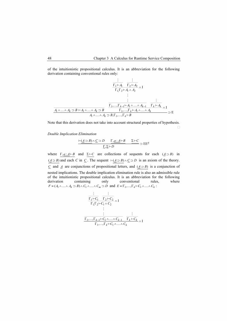
Chapter 3 A Calculus for Runtime Service Composition 48
of the intuitionistic propositional calculus. It is an abbreviation for the following derivation containing conventional rules only:
1 1 2 2
1, 2 1 2
1 1 1 1
1 1 1 1
1 1
I
, , I, , E
, , ,
k k k k
k k k k
k k
A AA A
A A AA A B A A B A A
A A B B
− −
Γ Γ∧
Γ Γ ∧
Γ Γ ∧ ∧ Γ∧
∧ ∧ ⊃ ∧ ∧ ⊃ Γ Γ ∧ ∧⊃
∧ ∧ ⊃ Γ Γ
0 00
0 00 0
0
… …… … … …
… …
Note that this derivation does not take into account structural properties of hypothesis.
Double Implication Elimination
( ) , :EE
,aA B C D a A B C
D
⊃ ∧ ⊃ Γ Σ⊃
Γ Σ
0 0
0
0
where , :a A BΓ 0 and CΣ0 are collections of sequents for each ( )A B⊃ in ( )A B⊃ and each C in C . The sequent ( )A B C D⊃ ∧ ⊃0 is an axiom of the theory. C and A are conjunctions of propositional letters, and ( )A B⊃ is a conjunction of nested implications. The double implication elimination rule is also an admissible rule of the intuitionistic propositional calculus. It is an abbreviation for the following derivation containing only conventional rules, where
and 1 1( )k mF A A B C C D≡ ∧ ∧ ⊃ ∧ ∧ ∧ ⊃… … 1 1E C, , k kC≡ Γ Γ ∧∧0… … :
1 1 2 2
1, 2 1 2
1 1 1 1
1 1
I
, , I, ,
k k k
k k
C CC C
C C CC C
− −
Γ Γ∧
Γ Γ ∧
Γ Γ ∧ ∧ Γ k ∧Γ Γ ∧ ∧
0 00
0 00
… …… …

3.2 Structural Synthesis of Programs 49
k
1
1 1
1 1 1 1
1 1 2
1
1
1
, : , , : I, : , , :
, : IE
, E, , , ,
ak k
k k k
ak
k
m
k
a A a A Ba A a A A B
a A A A BF F A A B
F C C D EF D
− −
Γ⊃
Γ ⊃
Γ ∧ ∧ ⊃⊃
Γ ∧ ∧ ⊃⊃
Γ ∧ ∧ ⊃⊃
Γ Γ Γ
00
00 0
00
……
………
…
Here we did also not take into account structural properties of hypothesis. Soundness and completeness proofs of the structural synthesis rules can be found in (Mints and Tyugu 1982) and (Matskin and Tyugu 2001).
3.2.6 Program Extraction for Structural Synthesis Rules Similar to the conventional rules of intuitionistic propositional logic we can introduce proof terms (i.e., realizations) into the structural synthesis rules. The structural synthesis rules with proof terms are as follows.
Table 6 SSR using proof terms (SSP)
Introduction Rules Elimination Rules
, : : I( : . ) :
uu A M Bu A M A Bλ
Γ ⊃⊃
00
: :
E:
M A B N A
M N B
Γ
Γ
⊃⊃
0 0
0
: ( ) , : : :
EE, ( : . , ) :
uF A B C D u A M B N C
F u A M N Dλ
⊃ ∧ ⊃ Γ Σ⊃
Γ Σ
0 0
0
0
As expected, proof term derivations (i.e., lambda term constructions) are carried along with the deductions. A sequent :M AΓ0 expresses the judgment “M is a proof term for A under hypothesis Γ”. In other words, M is a lambda term or program to compute an A from the inputs listed in Γ.
3.2.7 Example of a Proof with Program Extraction Let the propositional variables X, Y, Z, J, I represent objects of type real, denoted by respective small letters. The variable z depends on x and y, j depends on the functional dependency of z on y, and the variable i depends on the functional dependency of j on x. These dependencies can result, for example, from the following integration problem
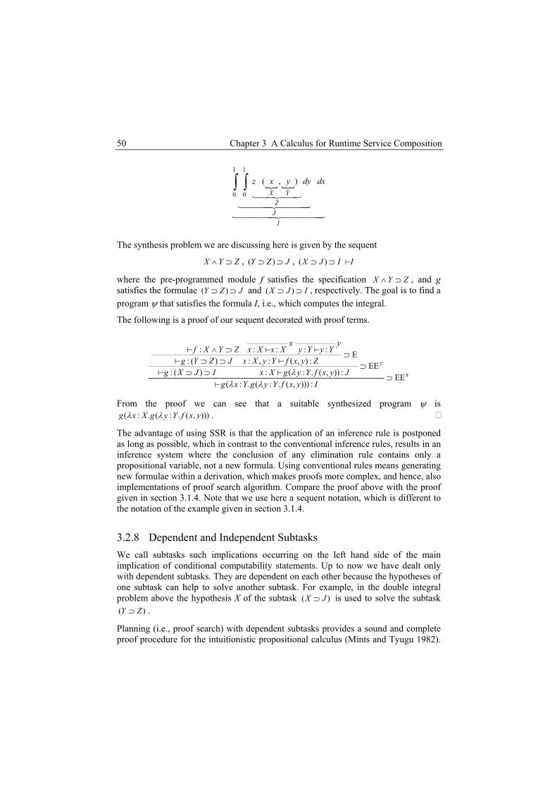
Chapter 3 A Calculus for Runtime Service Composition 50
1 1
0 0
( , )X Y
ZJ
I
z x y dy d∫ ∫ x
The synthesis problem we are discussing here is given by the sequent
X Y Z∧ ⊃ , ( )Y Z J⊃ ⊃ , ( )X J I⊃ ⊃ I0
where the pre-programmed module f satisfies the specification X Y Z∧ ⊃ , and g satisfies the formulae ( and ()Y Z J⊃ ⊃ )X J I⊃ ⊃ , respectively. The goal is to find a program ψ that satisfies the formula I, i.e., which computes the integral.
The following is a proof of our sequent decorated with proof terms.
: : : : : E: ( ) : , : ( , ) : EE
: ( ) : ( : . ( , )) : EE( : . ( : . ( , ))) :
y
x
x yf X Y Z x X x X y Y y Y
g Y Z J x X y Y f x y Zg X J I x X g y Y f x y J
g x Y g y Y f x y Iλ
λ λ
∧ ⊃ ⊃⊃ ⊃ ⊃
⊃ ⊃ ⊃
0 0 00 0
0 00
From the proof we can see that a suitable synthesized program ψ is ( : . ( : . ( , )))g x X g y Y f x yλ λ .
The advantage of using SSR is that the application of an inference rule is postponed as long as possible, which in contrast to the conventional inference rules, results in an inference system where the conclusion of any elimination rule contains only a propositional variable, not a new formula. Using conventional rules means generating new formulae within a derivation, which makes proofs more complex, and hence, also implementations of proof search algorithm. Compare the proof above with the proof given in section 3.1.4. Note that we use here a sequent notation, which is different to the notation of the example given in section 3.1.4.
3.2.8 Dependent and Independent Subtasks We call subtasks such implications occurring on the left hand side of the main implication of conditional computability statements. Up to now we have dealt only with dependent subtasks. They are dependent on each other because the hypotheses of one subtask can help to solve another subtask. For example, in the double integral problem above the hypothesis X of the subtask ( )X J⊃ is used to solve the subtask
. ( )Y Z⊃
Planning (i.e., proof search) with dependent subtasks provides a sound and complete proof procedure for the intuitionistic propositional calculus (Mints and Tyugu 1982).

3.2 Structural Synthesis of Programs 51
For problems involving a few dependent subtasks proof search can be done in feasible time. The general decision problem for the intuitionistic propositional calculus is P-SPACE complete, which has been proven by (Ladner 1977). For the worst case this of course means bad proof search behavior. Tyugu and Harf reported in (Tyugu and Harf 1980) another proof search strategy, which they called the mode of independent subtasks. Here, different subtasks cannot help each other. This strategy gives good planning performance but it is not applicable to problems as the double integral presented above. Mints has proven in (Mints 1991) that planning with independent subtasks leads to a sound and correct decision algorithm for a fragment of the modal logic S4 (Mints 1992) where only computability statements are considered, and A⊃B is understood as strict implication (A⊃B).
Inference rules for planning with independent subtasks are as follows:
Table 7 SSR for planning with independent subtasks
Introduction Rules Elimination Rules
, : : I( : . ) :
uu A M Bu A M A Bλ
Γ ⊃⊃
00
: :
E:
M A B N A
M N B
Γ
Γ
⊃⊃
0 0
0
: ( ) : : :
EEind( : . , ) :
uF A B C D u A M B N C
F u A M N Dλ
⊃ ∧ ⊃ Σ⊃
Σ
0 0 0
0
The rules and remain unchanged. The only difference from the rule Iu⊃ E⊃EEa⊃ of the SSR (cf. Table 6) is in the second premise of the rule EEinda⊃ : it does
not any longer share any formula with the antecedent of the conclusion. It was through these formula that other subtasks could help.
3.2.9 Proof Search Algorithm The proof search algorithm used in the SSP was described in (Tyugu and Harf 1980). Kanovich carried out a thorough study of a similar algorithm (Kanovich 1991). The proof search strategy of the SSP is assumption-driven forward as well as goal-driven backward search. Assumption-driven forward search is used to select computability statements. Goal-driven backward search is used to select subtasks. If the forward search cannot be continued, a subtask of a conditional computability statement, whose unconditional input variables are computed, is selected, i.e., a subproblem to be solved is generated for a negative occurrence of a sub-formula A⊃B. If the proof of the subtask succeeds, the next subtask of the same computability statement is selected. Otherwise, if the proof of the subtask fails, selecting a subtask of another conditional computability statement continues the proof. Subtasks are selected until either the goal is reached or no further subtask selection is possible.

Chapter 3 A Calculus for Runtime Service Composition 52
Example. Figure 3 shows a search tree of the double integration example from above. Each edge represents a step of the goal-driven backward search (i.e., subtask selection). Nodes represent assumption-driven search (i.e., computability statement selection). The dotted edge indicates backtracking.
Success
Find I
Select Y⊃Z from (Y⊃Z) ⊃J
Given Y, Find Z
Select X⊃J from (X⊃J) ⊃I
Given Y,X, Find J:Select X∧Y⊃Z
Select X⊃J from (X⊃J) ⊃I
Given X, Find J
Select Y⊃Z from (Y⊃Z) ⊃J
Given X,Y, Find Z:Select X∧Y⊃Z
Fail
Figure 3 Search tree to example double integration
An appropriate data structure, on which the proof search algorithm of SSP can be conducted, is a network that represents a set of computability statements Γ describing problem conditions. Uustalu and Tyugu describe in (Tyugu and Uustalu 1994) essentially the same data structure as higher-order functional constraint networks (HFCN) and show the relation to logic. In (Tyugu 1991a) Tyugu explains this data structure as higher-order dataflow schema (HODS). The nodes of HODSs are either functional nodes or control nodes. Control nodes receive subtasks as input. Control nodes exercise control over the execution order of their respective subtasks, but perform computations as well.
The data structure is built as follows. Every propositional variable becomes a node and every computability statement becomes either a functional or control node in the network. Each computability statement is connected with the nodes of propositional variables that occur in this formula. Hence, computability statements are connected with each other in the network through their common propositional variables. The direction of each edge is determined by the following rule that arrows must lead from negative occurrences of propositional variables to positive occurrences of propositional variables. A propositional variable occurs negative when it is on the left side of an odd number of implications in a formula. Otherwise the propositional variable occurs positive.
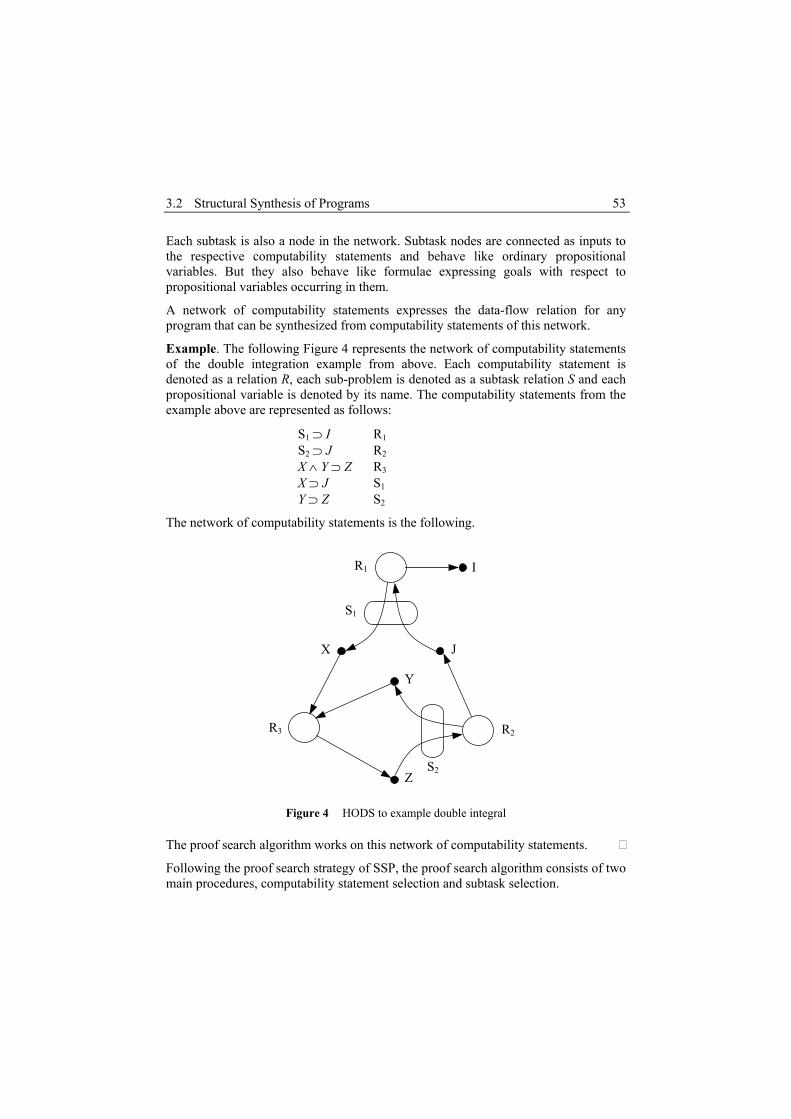
3.2 Structural Synthesis of Programs 53
Each subtask is also a node in the network. Subtask nodes are connected as inputs to the respective computability statements and behave like ordinary propositional variables. But they also behave like formulae expressing goals with respect to propositional variables occurring in them.
A network of computability statements expresses the data-flow relation for any program that can be synthesized from computability statements of this network.
Example. The following Figure 4 represents the network of computability statements of the double integration example from above. Each computability statement is denoted as a relation R, each sub-problem is denoted as a subtask relation S and each propositional variable is denoted by its name. The computability statements from the example above are represented as follows:
S1 ⊃ I R1 S2 ⊃ J R2 X ∧ Y ⊃ Z R3 X ⊃ J S1
Y ⊃ Z S2
The network of computability statements is the following.
S2
S1
R1
Z
Y
X
I
J
R3 R2
Figure 4 HODS to example double integral
The proof search algorithm works on this network of computability statements.
Following the proof search strategy of SSP, the proof search algorithm consists of two main procedures, computability statement selection and subtask selection.

Chapter 3 A Calculus for Runtime Service Composition 54
Computability statement selection. When the proof search algorithm works in the forward direction only unconditional computability statements are considered. If a computability statement has been applied then its output variables (i.e., propositional variables of its conclusion) are marked as computable and the computability statement is discharged. Variables that are marked as computable are used to check if other computability statements, where these variables serve as input variables, become applicable. A computability statement is applicable if all its input variables are computable. Applicability can easily be checked using input-variable-counters, which are initialized with the number of input variables and counted down as the input variables become computable. The search becomes a simple flow analysis on the network of computability statements, where all necessary computability statements are discharged one after another until the goal is reached or no further step is possible. This search can be done in linear time.
Subtask selection. Subtask selection is only applied if the computability statement selection cannot be continued (i.e., the goal has not been reached but no further step is possible). In this case, a subtask of a conditional computability statement, whose unconditional input variables are computable, is selected. For each selected subtask, a subproblem is generated. If the proof of a subproblem succeeds then the next subtask of the current computability statement is selected and a new subproblem is generated and so on. If the proof of a subproblem fails, a subtask of another conditional computability statement is selected and the process is repeated. Subtasks of conditional computability statements are selected and subproblems are generated until the goal is reached or no further subtask selection is possible.
3.2.10 Branch Control Structures in SSP In SSP it is possible to express disjunction. However, disjunction in SSP has to be encoded in modules with subtasks, which can lead to a huge amount of additional modules. Practically, a programmer has to use his intuition to guess in advance how a disjunction could be used in the programs to be synthesized in order to provide a reasonable set of modules providing the branch control structure. In principle, expressing disjunction in SSP means applying the transformation rule (cf. 3.2.3, elimination of disjunction) for rewriting disjunctions. The result of such a transformation is a specification of a module with subtasks, where the branch is chosen inside the module.
Example. Consider the following formulae:
: , : , :f A B C g B D h C D⊃ ∨ ⊃ ⊃ .
If we apply the transformation rule for rewriting disjunctions we obtain a new specification instead of :f A B C⊃ ∨ , where the body of the function f´ calls the function f and chooses one of the subtasks (i.e., branches) depending on what f computes.

3.3 Extended Structural Synthesis of Programs 55
' : ( ) ( )f A B D C D D∧ ⊃ ∧ ⊃ ⊃
Depending on A, either the subtask B ⊃ D or the subtask C ⊃ D will be used to compute D. The module f´ constructed for the new specification
( ) ( )A B D C D D∧ ⊃ ∧ ⊃ ⊃ realizes the disjunction B ∨ C inside, i.e., the programmer must supply the branch control structure. Note, however, the implementation of each branch will be synthesized.
The following section describes an extension of the SSP technique, which is called the extended structural synthesis of programs (ESSP). The ESSP defines a framework for adding the disjunction connective to the logical specification language of SSP. Consequently, rewriting of disjunction in advance is not needed any longer. In contrast to the SSP, a branch control structure needs not to be pre-programmed. Nevertheless, as we will show, the transformation rule for rewriting a disjunction is used just in time in the extended proof search algorithm of ESSP.
3.3 Extended Structural Synthesis of Programs
At the beginning of Chapter 3 we mentioned that the extended structural synthesis of programs includes three extensions to the SSP, introduction of disjunction into the logical language, introduction of quantifiers in a restricted way in order to keep proof search efficient, and adding falsity to the logical language. While the need for disjunction is intuitively clear, namely because pre-programmed modules may throw exceptions, the reason for using quantifiers and falsity may be not so.
Let us justify the use of quantifiers and falsity. In pure SSP synthesis is carried out in a single structure where all objects are explicitly specified. We can think of such a structure as a class in an object-oriented language, see (Tyugu 1994) for instance. It is our intention to use the structural synthesis method to compose services from components, where components become known only at synthesis time, not at specification time. This requires a language where we can state that a component with particular properties exists or, vice versa, is required, which makes the use of quantifiers unavoidable. The use of falsity is simply motivated by the fact that we would like to be able to specify that we want to abort the execution of a program or branch after exception handling or when an exception occurs.
Example. Suppose that a server controls access to a printer and that a client wishes to use it. We can consider the server and the client as separate components. In the original state only the server component itself has access to the printer. After composition with the client component, the printer access is transferred to a new component that realizes a print service for this particular client. Figure 5 shows this scenario.

Chapter 3 A Calculus for Runtime Service Composition 56
Before synthesis After synthesis
Figure 5 Components before and after synthesis to example print service
Server
: . ( ): . ( )
: . ( ). ( )
: . ( ):
f FN a F at b F b FTcn d PT d FT
w C w CErp r PR r IRnoc CE
⊃ ∃∀ ⊃
∀ ∧ ⊃∃ ∨
∀ ⊃⊃⊥
Client : . ( ): , . ( ) ( ): . ( )
:
pt x PT xcv y c F y C c Op O z PR z PEerror PE
⊃ ∃∀ ∧ ⊃
⊃ ∃ ∨⊃⊥
:ps FN IR⊃
Printer
: . ( ): , . ( ) ( ): . ( )
:
pt x PT xcv y c F y C c Op O z PR z PEerror PE
⊃ ∃∀ ∧ ⊃
⊃ ∃ ∨⊃⊥
: . ( ): . ( )
: . ( ). ( )
: . ( ):
f FN a F at b F b FTcn d PT d FT
w C w CErp r PR r IRnoc CE
⊃ ∃∀ ⊃
∀ ∧ ⊃∃ ∨
∀ ⊃⊃⊥
Client Server
Printer
In the extended structural synthesis of programs computability statements can express properties of the server and client component as follows: the server can provide information about the printer type : . (pt x PT x)⊃ ∃
: , . ( ) ( )y c F y C c
; provided with some file object F(y) and converter object C(c) the server can convert the file object into a printable format O, which is expressed by cv O∀ ∧ ⊃ ; the server can print an object
where an exception PE might occur or a print report object PR(z) is returned; in case of exception PE we abort the print job with ; the client can compute a file object F(a) from a filename FN by
: . ( )p O z PR z PE⊃ ∃ ∨:error PE ⊃⊥
: . ( )f FN a F a⊃ ∃ ; having a file object we can compute the corresponding file type FT by
; from the file type and having a printer type object PT(d) by executing the module cn the client can obtain a suitable converter object C(w) or a converter is not available for that file-printer type combination, which is expressed by exception CE; in case of exception CE we abort the print job with noc ;and finally, from any print report object PR(r) the client can compute by its internal print report IR.
: . ( )t b F b FT∀ ⊃: . . (d PT w∃
⊃⊥: . (r PR r∀
( )d FT w C∀ ∧ ⊃
) IR⊃
) CE∨
CE:rp
The common properties that are expressed by predicates and quantifiers occurring in computability statements of the client and server component allow us to compose both components into a print service satisfying the computability statement , which would not be possible otherwise. Compiling modules of components into a program at runtime gives flexibility in terms of extensibility. For instance, we could think of adding at runtime a server extension providing monitoring and security features to be executed while accessing the printer, which is not possible when compiling the server component into a service in the traditional way.
:ps FN IR⊃

3.3 Extended Structural Synthesis of Programs 57
In the extended structural synthesis of programs the disjunction connective is added to the logical language LL. This extension enables us to synthesize branch control structures. Hence, pre-programmed modules implementing branch control structures are not needed. Also, the flexibility to reuse modules increases, because building blocks implementing a branch of a module can now be represented as individual, independent modules.
Tyugu and Harf also proposed an approach to synthesis of branch control structures in (Tyugu and Harf 1980). They used a simplified disjunction elimination rule for the construction of a proof. This rule allows synthesizing partial programs that throw an exception when the problem cannot be solved for certain initial data. In order to be able to synthesize programs that are complete with respect to their branches, an additional inference rule is needed. Moreover, a program derivation rule for extracting branches is also needed.
3.3.1 Logical Language LL of ESSP The logical language of the extended structural synthesis of programs extends the logical language of the SSP in the following way: 1) the disjunction connective may occur on the right-hand side of the main implication of a formula, 2) monadic predicates may be used but predicate variables must not occur free; variables are bound by universal quantifier if they occur on the left-hand side of an implication and existential quantifier if they occur on the right-hand side of an implication, and 3) the falsity constant may occur but exclusive on the right-hand side of the main implication of a formula.
The general form of an admissible formula in ESSP can be defined as follows:
. ( . . ) .1 1 1 1 1
i iij i j ij
i
n ln m kx u U v V X y Y
i j j i j
ZW
∀ ∀ ⊃ ∃ ∧ ⊃ ∃ = = = = =
∧ ∧ ∧ ∨ ∧
where n, m ≥ 0, ni ≥ 1, k, li ≥ 1, the Uij’s, Vi’s, Xj’s, and Yij’s are propositional variables or monadic predicates whose individual variables of predicates do not occur free, W may be the falsity constant ⊥, x, u are lists of the individual variables of the predicates Xj and Uij (if they are predicates), and v, y are individual variables of the predicates Vi and Yij (if they are predicates). We use [⋅] to denote that a respective quantifier must be given only if some Uij, Vi, Xj, or Yij is a predicate. An empty premise of an implication is identified with ⊤. New propositional variables W and Zi

Chapter 3 A Calculus for Runtime Service Composition 58
and axioms W and 1
i
k
i⊃
=∨ Z ij.
1
ii
lZ y Y
j⊃ ∃
=∧ can substitute the sub-formula on the
right-hand side of the main implication.
3.3.2 Inference Rules As the SSP, the ESSP uses intuitionistic logic, which guarantees constructiveness of the found proofs. The logical language LL allows writing formulae containing implication, conjunction, disjunction, and falsity as well as quantifiers but only in a restricted way. It is thus sufficient to use introduction and elimination rules for implication and conjunction, the elimination rule for disjunction, elimination and introduction rules for universal and existential quantifiers, and the elimination rule for falsity. As for the SSP, inference rules are used for deriving a proof of a formula. Leaves in the derivation tree represent axioms while inner nodes are inference steps, where one of the inference rules is applied and a new formula is derived.
The localized version of natural deduction rules for the ESSP is shown in Table 8 below. The rules for handling implications and conjunction are the same as presented in chapter 3.1.3.2. Note that introduction and elimination rules with multiple premises given in Table 8 make use of structural properties of hypothesis. Compare with section 3.1.3.2.
Table 8 Conventional inference rules (ESSP)
Introduction Rules Elimination Rules
IA BA B
Γ ΓΓ
∧∧
0 00
LEA BA
ΓΓ
∧ ∧00 REA B
BΓ
Γ∧ ∧0
0
no ∨ introduction , , : , : Eu wA B u A C w B CC
Γ Γ ΓΓ
∨ ∨0 0 00
, : Iuu A BA B
ΓΓ
⊃⊃0
0 EA B A
BΓ Γ
Γ⊃ ⊃0 0
0
no 3 introduction EC
ΓΓ
00
3 3
[ / ] I.
aa x Ax A
Γ∀
Γ ∀00
. E[ / ]
x At x A
Γ ∀∀
Γ0
0
[ / ] I.
t x Ax A
Γ∃
Γ ∃00
,. , :[ / ] Ea ux A u a x A CC
Γ ∃ Γ∃
Γ0 0
0

3.3 Extended Structural Synthesis of Programs 59
3.3.3 Program Extraction Each formula of the logical language LL has a computational meaning. However, computational meanings of formulae of the logical language of SSP are kept in ESSP. Again, we use Kleene realizability of intuitionistic formulae, and associate a term (i.e., program or pre-programmed module) with each derivable formula or axiom.
As before, we use [⋅] to denote a respective quantifier that must be given only if a predicate occurs. The logical language LL of ESSP is extended with terms to LL1 as follows.
1) A propositional variable corresponds to an object variable , where A is a propositional variable and a is the corresponding object.
Aa :
2) A predicate P(x) corresponds to an object.
3) An unconditional computability statement has a computational interpretation as a function f for computing some bj from ai’s, i.e., ai’s are inputs and bj’s are possible outcomes of f. Hence, f indicates which bj has been computed:
11 1
... . : . i j
n m
ni j
a a f a A Bλ= =
∀ ⊃ ∧ ∨
Note that the Bj’s may have the form 1
.jl
jii
b B=
∃ ∧ where l ≥ 1.
4) A conditional computability statement denotes the computability of some yj’s depending on xj’s and on the computation of all vi’s from uij’s. Hence,
1 11 1 1
... ... . : . ( . . )inn m
n m ij i ji j j j 1
k
jg g x x f x u U v V X Yλ= = = =
∀ ∀ ⊃ ∃ ∧ ⊃ ∧ ∧ ∧ ∨
or
1 11 1 1
... ... . : . ( . . )inn m
n m ij i ji j j
g g x x f x u U v V Xλ= = =
∀ ∀ ⊃ ∃ ∧ ∧ ∧ ∧ ⊃ ⊥
where Yj’s may have the form 1
.jl
jii
y Y=
∃ ∧ (l ≥ 1) and gi, i = 1, …, n, are functional
variables denoting realizations ei of subtasks that should be synthesized:
11
... . : . .i
i
n
i in i ijj
u u e u U v Vλ=
∀ ⊃ ∃ i ∧ .
In order to extract programs from constructive proofs we need to extend the inference rules according to the language LL1. The inference rules for conjunction introduction
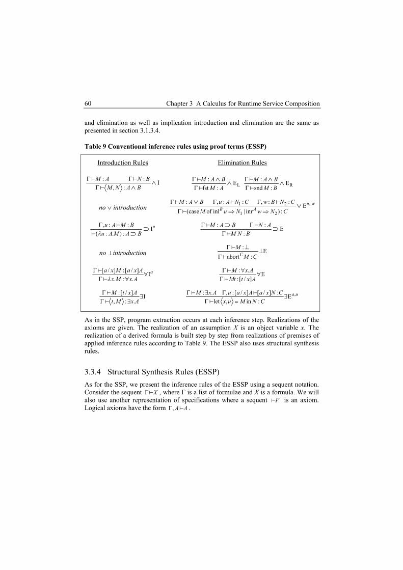
Chapter 3 A Calculus for Runtime Service Composition 60
and elimination as well as implication introduction and elimination are the same as presented in section 3.1.3.4.
Table 9 Conventional inference rules using proof terms (ESSP)
Introduction Rules Elimination Rules
: : I, :
M A N BM N A B
Γ ΓΓ
∧∧
0 00
L: E
fst :M A B
M AΓΓ
∧ ∧00
R: E
snd :M A B
M BΓΓ
∧ ∧00
no ∨ introduction , 1 2
1 2
: , : : , : : E(case of inl | inr ) :
u wB A
M A B u A N C w B N CM u N w N C
Γ Γ Γ
Γ ⇒ ⇒
∨ ∨0 0 0
0
, : : I( : . ) :
uu A M Bu A M A Bλ
Γ ⊃⊃
00
: : E:
M A B N AM N B
Γ ΓΓ⊃ ⊃0 00
no 3 introduction : E
abort :CM
M CΓ
Γ
0
0
3 3
[ / ] :[ / ] I. : .
aa x M a x Ax M x Aλ
Γ∀
Γ ∀0
0 : . E
:[ / ]M x A
Mt t x AΓ ∀
∀Γ
00
:[ / ] I, : .
M t x At M x A
Γ∃
Γ ∃0
0 ,: . , :[ / ] [ / ] : E
let , in :a uM x A u a x A a x N C
x u M N CΓ ∃ Γ
∃Γ =
0 00
As in the SSP, program extraction occurs at each inference step. Realizations of the axioms are given. The realization of an assumption X is an object variable x. The realization of a derived formula is built step by step from realizations of premises of applied inference rules according to Table 9. The ESSP also uses structural synthesis rules.
3.3.4 Structural Synthesis Rules (ESSP) As for the SSP, we present the inference rules of the ESSP using a sequent notation. Consider the sequent XΓ , where Г is a list of formulae and X is a formula. We will also use another representation of specifications where a sequent is an axiom. Logical axioms have the form
0F0
, A AΓ 0 .

3.3 Extended Structural Synthesis of Programs 61
We have already discussed admissible inference rules (SSR) employed by the SSP in section 3.2.5. The SSR used in pure SSP are:
Implication Introduction
, : Iuu A BA B
ΓΓ
⊃⊃0
0
Implication Elimination
EA B A
B
Γ
Γ
⊃⊃
0 0
0
Double Implication Elimination
( ) , :EE
,aA B C D a A B C
D
⊃ ∧ ⊃ Γ Σ⊃
Γ Σ
0 0
0
0
In addition to these three admissible inference rules, the ESSP introduces an admissible inference rule for disjunction elimination. We will also use inference rules for universal and existential elimination, and falsity elimination but we do not use universal and existential introduction. However, the inference rules for falsity, universal, and existential elimination remain unchanged.
Disjunction elimination
We will represent the inference rule for disjunction in the simplified language where a disjunction can appear only in the unconditional computability statement. For
convenience, the simplified sub-formula A∨B is used instead of 1
ni
iA
=∨ . However, the
generalization to the case of infinitely many disjuncts is straightforward. The structural synthesis rule for disjunction elimination is then formulated as follows
, , : , :E
, ,u wW A B W u A C w B C
C
⊃ Γ Σ ∆
Γ Σ ∆
∨∨
0 0 0 0
0
where W A B⊃ ∨0 is an axiom (i.e., computability statement), and WΓ0 is a collection of sequents, one for each W in W . Our structural synthesis rule for disjunction elimination is an admissible rule of the intuitionistic calculus. It is an abbreviation for the following derivation containing conventional rules only.

Chapter 3 A Calculus for Runtime Service Composition 62
1 1 2 2
1, 2 1 2
1 1 1 1
1 1 1 1
1 1
,
1 1
I
, , I, , E
, , , (*)
(*) , : , : E, , , , ,
k k k k
k k k k
k k
u w
k k
W WW W
W W WW W A B W W A B W W
W W A B A B
u A C w B CW W A B C
− −
Γ Γ∧
Γ Γ ∧
Γ Γ ∧ ∧ Γ∧
∧ ∧ ⊃ ∨ ∧ ∧ ⊃ ∨ Γ Γ ∧ ∧⊃
∧ ∧ ⊃ ∨ Γ Γ ∨
Σ ∆ ∨∧ ∧ ⊃ ∨ Γ Γ Σ ∆
0 00
0 00 0
0
0 00
… …… … … …
… …
… …
For convenience, we have divided this derivation into to parts. The * of the first part indicates that this part of the derivation continues at * of the second part. The derivation above does not take into account structural properties of hypothesis.
3.3.5 Program Extraction for Structural Synthesis Rules (ESSP) As for the SSP, we can introduce proof terms (realizations) into the structural synthesis rules of the ESSP. The structural synthesis rules with proof terms are shown in Table 10.

3.3 Extended Structural Synthesis of Programs 63
Table 10 SSR using proof terms (ESSP)
Introduction Rules Elimination Rules
, : : I( : . ) :
uu A M Bu A M A Bλ
Γ ⊃⊃
00
: :
E:
M A B N A
M N B
Γ
Γ
⊃⊃
0 0
0
: ( ) , : : :
EE, ( : . , ) :
uF A B C D u A M B N C
F u A M N Dλ
⊃ ∧ ⊃ Γ Σ⊃
Γ Σ
0 0
0
0
no ∨ introduction 1 2 ,
1 2
: : , : : , : :E
, , (case of inl | inr ) :u w
B A
M W A B N W u A N C w B N C
M N u N w N C
⊃ Γ Σ ∆
Γ Σ ∆ ⇒ ⇒
∨∨
0 0 0 0
0
no 3 introduction : E
abort :CM
M CΓ
Γ
0
0
3 3
no ∀ introduction : . E:[ / ]
M x AMt t x A
Γ ∀∀
Γ0
0
no ∃ introduction ,: . , :[ / ] [ / ] : E
let , in :a uM x A u a x A a x N C
x u M N CΓ ∃ Γ
∃Γ =
0 00
As for the SSP, proof term derivations (i.e., lambda term constructions) are carried along with deductions. A sequent :M AΓ0 again expresses the judgment “M is a proof term for A under hypothesis Γ”.
3.3.6 Proof Search Algorithm Extension for Disjunction The basic proof search algorithm of SSP is kept in ESSP. In order to deal with disjunctions in logical specifications, the extended proof search algorithm rewrites logical specifications containing the disjunction connective dynamically. A logical axiom with a disjunction is rewritten into the form of SSP’s specification language if and only if during proof search the axiom has to be applied. The proof will then be continued with the new set of formulae. For each rewritten axiom, a realization deploying the module in the rewritten form has to be synthesized. This is different from SSP where the specification containing the disjunction connective has to be

Chapter 3 A Calculus for Runtime Service Composition 64
rewritten in advance and modules for the rewritten specifications have to be supplied by a user.
Let us introduce the notion of the innermost goal. A theory in our logic consists of a finite set of propositional variables and of computability statements describing problem conditions. If the set of computability statements consists of unconditional computability statements only, the innermost goal is the goal stated in a given synthesis problem Γ , i.e., the innermost goal is G. If Γ also contains conditional computability statements, a search-tree with backtracking may result. A subtask
G0
( )A B⊃ in the search tree induces the specification of the current subproblem , A BΓ 0 where Γ includes all hypotheses and already derived formulae, and B is the innermost goal. In other words, the innermost goal is the goal of the current subtask to be solved.
Example. Consider again the double integral example described in section 3.2.7. The search tree annotated with innermost goals (i.e., the consequents of the sequents at respective nodes) is the following:
Success
Γ ⊢ I
Select Y⊃Z from (Y⊃Z) ⊃J
Γ,Y ⊢ Z
Select X⊃J from (X⊃J) ⊃I
Γ,X ⊢ J
Select X⊃J from (X⊃J) ⊃I
Γ,X ⊢ J
Select Y⊃Z from (Y⊃Z) ⊃J
FailΓ,Y ⊢ Z
Figure 6 Search tree with innermost goals to example double integration
Let us denote by f the realization of a specification of the form
1:
n
ii
f L A=
⊃ ∨
where each Ai is a propositional variable and i ranges over 1, …, n (n≥2), and L is any admissible left-hand side of the main implication of ESSP-formulae.

3.3 Extended Structural Synthesis of Programs 65
Let us assume that the propositional variable G is the innermost goal of the problem to be solved, and then the computability statement of f has to be rewritten into the form
1' : ( ) ( )nf L A G A G G∧ ⊃ ∧ ∧ ⊃ ⊃…
where G is a propositional variable of the theory and identifies the innermost goal of the current problem to be solved. The realization of the new specification is f´. The construction of f´ is straightforward:
11 1case of inl | | inrnA A
n nf N a s a⇒ ⇒… s
where N is a list of realizations, one for each subformula in L, and 1, , ns s… denote the subtask-realizations of the conditionals 1( ), ,( n )A G A G⊃ ⊃… .
Dynamic rewriting of a formula with a disjunction in its conclusion enables us to efficiently derive a proof of a goal formula from axioms containing disjunction in their respective conclusion, because the proof search algorithm of the SSP requires only minor changes.
3.3.7 Proof Search Algorithm Extension for Quantifier Elimination The structural synthesis rules of the ESSP use only the eliminations rules for quantifiers; moreover, predicates of our logical language may have only a single individual variable. These two facts enable us to design an efficient proof search algorithm including quantifier elimination. In principle, unification reduces to substitution of a single predicate variable. Hence, universal quantifier elimination requires only substitution of constant for a variable. The proof search extension for existential quantifier elimination is similar to the one for disjunction.
To keep the complexity of proof search as low as possible we use the strategy of postponing quantifier elimination as long as we can. That is, proof search first applies unconditional computability statements; if the goal has not been proven it continues with conditional computability statements, and only if the goal has still not yet been reached, it continues we with quantifier elimination.
Let us denote the realization of an existentially quantified predicate by r. The formula has the form
: . ( )r x P x∃
where P is a monadic predicate with the individual variable x.
Let us assume that the propositional variable G is the innermost goal of the current problem to be solved. According to the existential quantifier elimination rule and following our strategy for disjunction elimination, we can eliminate this quantifier if we can prove the new goal , where a is a new parameter and a does not occur free in G, or in a hypothesis of the sub-derivation of G, other than P(a).
( )P a GΓ ⊃0

Chapter 3 A Calculus for Runtime Service Composition 66
In order to derive G from there must be some axiom of the from: ( )P aΓ ∪
: . ( )f y P y L A∀ ∧ ⊃ ,
where L is any (possibly empty) admissible sub-formula of the left-hand side of the main implication of a formula of our logical language, y must not occur free in L and A, and A is an admissible right-hand side of the main implication of a formula. Before we apply universal quantifier elimination, L must have been derived, and some P(a) must be given. The universal quantifier elimination gives:
: ( )f P t L A∧ ⊃
Substituting a for t allows us eliminate the existential quantifier, provided we can proof G from A
3.3.8 Example of Synthesis with Program Extraction Let us show the proof and the program extraction for the printer example, which we have introduced at the beginning of the subsection 3.3. We gave already some intuitive meaning of the computability statements of the server and client. The fact that the server and client are two components is inessential here; we will discuss logical aspects only. This example illustrates logical features added to the structural synthesis of programs.
Consider the interpretation of propositional variables O, PE, FN, FT, CE, and IR, and the interpretation of predicates PT, F, C, and PR.
O is a propositional variable which represents an object variable that depends on objects represented by the predicates F(y) and C(c).
PE is a propositional variables that represent an object variable that depends on the object variable represented by the propositional variable O.
FN is a propositional variable that represents an object variable that does not depend on any other object variable.
FT is a propositional variable which represents an object variable that depends on the object represented by the predicate F(b).
CE is a propositional variable which represents an object variable that depends on the object represented by the predicate PT(d) and the object variable represented by the propositional variable FT.
IR is a propositional variable which represents an object variable that depends on the object represented by the predicate PR(r).
PT is a predicate which represents an object that depends on nothing.
F is a predicate which represents an object that depends on and the object variable represented by the propositional variable FN.

3.3 Extended Structural Synthesis of Programs 67
C is a predicate which represents an object that depends on that depends on the object represented by the predicate PT(d) and the object variable represented by the propositional variable FT.
PR is a predicate that represents an object that depends on the object variable represented by the propositional variable O.
Now consider the axioms:
: . ( ); : , . ( ) ( ) ; : . ( ): ; : . ( ); : . ( ) ; : ;
: . ( ) . ( ) ; : . ( )
pt x PT x cv y c F y C c O p O z PR z PEerror PE f FN a F a t b F b FT noc CEcn d PT d FT w C w CE rp r PR r IR
⊃ ∃ ∀ ∧ ⊃ ⊃ ∃ ∨⊃⊥ ⊃ ∃ ∀ ⊃ ⊃⊥
∀ ∧ ⊃ ∃ ∨ ∀ ⊃
0 0 00 0 0 00 0
;
Each axiom represents a computability statement where the identifier to the left of the colon of an axiom denotes the respective pre-programmed module satisfying the formula to the right of the colon. These axioms are sufficient for deriving the goal
, i.e., to find a program ps that satisfies the formula FN IR⊃0 FN IR⊃ . The proof is presented below. We avoid showing proof terms of disjunctions. Instead, we present proof terms for the rewritten computability statements.
: . ( ) . ( ) E: ( ) . ( )
I ' : ( ) ( . ( ) ) ( )
cn d PT d FT w C w CEcn PT s FT w C w CE rw
cn PT s FT w C w IR CE IR IR
∀ ∧ ⊃ ∃ ∨∀
∧ ⊃ ∃ ∨≡ ∧ ∧ ∃ ⊃ ∧ ⊃ ⊃
00
0
: . ( ) E: ( ) : ( ) : ( ) E
II : ( ) ( ) :
t b F b FTqq F q q F q t F x FT
q F q t q FT
∀ ⊃∀
⊃⊃
≡
00 0
0
:: : E: ( ) : E
: ( ) : IIII : . ( ) :
IRk
IR
knoc CEce CE ce CE
ce CE noc ce
ce CE abort noc ce IR
k CE abort noc ce CE IRλ
⊃⊥⊃
⊥⊥
⊃≡ ⊃
000
0
0
: , . ( ) ( ) E: ( ) : ( ): ( ) ( ) : ( ), : ( ) : ( ) E
** : ( ), : ( ) ( , ) :
cv y c F y C c O hq F q q F qcv F i C j O q F q h C v h C v
q F q h C v cv q h O
∀ ∧ ⊃∀
∧ ⊃⊃
≡
000 0
0
,
: . ( ) E: ( ) : ( ) : ( ) E
: . ( ) : . ( ) : ( ) ( ) : E: . ( ) let in ( ) : I
*** : . ( ).let in ( ) : . ( )
m n
u
rp r PR r IRnn PR m n PR m rp PR e IRu
g z PR z g z PR z n PR m rp n IRg z PR z n g rp n IR
g z PR z n g rp n z PR z IRλϒ
∀ ⊃∀
⊃⊃
∃ ∃ ∃∃ =
⊃≡ ∃ = ∃ ⊃
00 0
0 00
0
:: : E: ( ) : E
: ( ) : I**** : . ( ) :
IRz
IR
zerror PEpe PE pe PE
pe PE error pepe PE abort error pe IR
z PE abort error pe PE IRλΦ
⊃⊥⊃
⊥⊥
⊃≡ ⊃
000
0
0

Chapter 3 A Calculus for Runtime Service Composition 68
: . ( )* ' : ( . ( ) ) ( )
p O z PR z PE rwp O z PR z IR PE IR IR
⊃ ∃ ∨≡ ∧ ∃ ⊃ ∧ ⊃ ⊃
00
,
,
E I I* * * * * * * * * * EE
: ( ), : . ( ) : . ( ) : ( ), : ( ) '( ( , ), , ) : E: ( ) '( ( , ), , ) :
IV : ( ) : . ( ). '( ( , ), , ) : . ( )
u zu z
v h
rwl
q F q l w C w l w C w q F q h C v p cv q h IRq F q let h l in p cv q h IR
q F q l w C w let h l in p cv q h wC wλΨ
⊃ ⊃ ⊃⊃
∃ ∃ ϒ Φ∃
= ϒ Φ≡ ∃ = ϒ Φ ∃ ⊃
0 00
0Il
IR⊃
,
,
E I I: . ( ) I II : ( ) : ( ) III IVE E
: . ( ) : ( ), : ( ) '( , ( ), , : . ( )) : EV : ( ) '( , ( ), , : . ( )) :
k l
k lIR
r rIR
rw rpt x PT x r PT r r PT r
pt x PT x q F q r PT r cn r t q k CE abort noc ce IR
q F q let r pt in cn r t q k CE abort noc ce IR
λ
λ
⊃ ⊃ ⊃⊃ ∃
⊃ ⊃∃ Ψ
∃≡ = Ψ
0 00 0
0
E
,
,
: . ( ) : : E E: ( ) : . ( ) V E
: ( ) '( , ( ), , : . ( )) : I: . ( ) '( , ( ), , : . ( )) :
r r
q qIR
uIR
uf FN a F a fn FN fn FN
fn FN f fn a F a
fn FN let q f fn in let r pt in cn r t q k CE abort noc ce IR
fn FN let q f fn in let r pt in cn r t q k CE abort noc ce FN IR
λ
λ λ
⊃ ∃⊃ ∃
∃∃
= = Ψ⊃
= = Ψ ⊃
0 00
0
0
From the proof we can see that a suitable program ps that satisfies the formula is FN IR⊃ : . ( ) '( , ( ), , : . ( ))IRfn FN let q f fn in let r pt in cn r t q k CE abort noc ceλ λ= = Ψ .
Note that our certainty about ps having to equal the value of the printing result relies on the fact that we used types (i.e., formulae) as identifiers of conceptual roles of values. Had we used the types as identifiers for ranges of values (like real or integer), our synthesis problem would have lost the information of the intended usage of the computability statements and ps could have been almost any program.

Chap t e r 4
Specification Language
In this section we describe a language for specifying components and services. This specification language has a straightforward translation into our logic. Our aim in designing the specification language has been to make it as convenient as possible for a software developer. This language should allow a simple and exact translation into a language of logic used in the synthesis process, but we have tried to avoid excessive use of logical notations. We present the semantics of the language by describing its translation into logic.
A specification may describe a component, a service, or a location, where location refers to a service point. We will subsequently use the word component as synonym for services and locations as well.
We introduce metainterfaces as logical specifications of components. Metainterfaces can be used in two ways: (i) as specifications of computational usage of components or (ii) as specifications of new components composed of components already supplied with metainterfaces.
A metainterface is a specification that:
Introduces a collection of interface variables of a component,
Introduces axioms showing the possible computations provided by realizations of the components, in particular, which interface variables are computable from other variables under which conditions. In an object-
69

Chapter 4 Specification Language 70
oriented language we can think of components as classes and realizations as methods and constructors for instance,
Introduces metavariables that implicitly connect different metainterfaces and reflect mutual needs of components on the conceptual level.
For describing the syntax, we rely on a meta-notation similar to the Backus-Naur Form that is commonly employed for language definitions. Keywords and symbolic constants appear inside quotes. Optional expressions are enclosed in square brackets.
4.1 Core of the Language
In this subsection we describe the syntactic constructs of specifications. We shall use example instances of specifications where it helps to illustrate our specification language.
The core of our specification language allows declaring interface variables, constants, bindings, and axioms.
:: '{' '}'
::
:: ( | | | ) [', ' ]
Metainterface MetaInterfaceName Specification
MetaInterfaceName Identifier
Specification InterfaceVariable Constant Binding Axiom Specification
=
=
=
The MetaInterfaceName is the name of the metainterface being declared.
Example. Assume we want to specify a component Exchange. Its metainterface declaration starts as follows:
Exchange { ... }
4.1.1 Interface Variables Specification of an interface variable is a declaration of the form:
:: ' :: 'InterfaceVariable Identifier Specifier= ,
where the is a name of the new interface variable being declared, and the is one of the following:
IdentifierSpecifier
Any of the primitive types of the underlying programming language (e.g., int, float ),

4.1 Core of the Language 71
A name of a metainterface,
A component name. :: ' int' | | ' float' | |Specifier MetaInterfaceName ComponentName= …
Operationally it denotes that, if the variable is used in composition, it will require a realization as a variable in the final program. Logically, such a declaration introduces a propositional variable with a name given by the . Identifier
Example. The interface variables currency, localCurrency, and exchangeRate are introduced into the metainterface Exchange:
Exchange { currency :: String, localCurrency :: String, exchangeRate :: float }
4.1.2 Constants Specification of a constant is a declaration of the form
:: '{' '}'Constant InterfaceVariable val= ,
where refers to a constant of the target programming language. val
Operationally this declaration states that, if the constant is used in the composition of a program, it will require a realization as an object, which is a constant in the final program and whose value is determined by . Logically, this declaration identifies an implication with an empty left-hand side.
val
4.1.3 Bindings A binding is an equality of the form
:: [. ]
:: ' '
Name Identifier Name
Binding Name Name
=
= =
denoting that realizations of the two interface variables must have equal values.
Name may be an identifier or a compound name, e.g., a.b.c denoting the interface variable c of the interface variable b of the interface variable a.
Example. A metainterface can be used for specifying how an application should be composed from components that are supplied with metainterfaces. In this case, a new component can be built completely from a specification of its metainterface. For this purpose, specifying equality relations (i.e., bindings) between some interface

Chapter 4 Specification Language 72
variables of the new component may be needed. Here we present a metainterface for calculating exchange rates that uses the metainterfaces Exchange defined above as component.
ExchangeRate { currency :: String, exchangeRate :: float, exch :: Exchange, exch = (Exchange), exch.currency = currency, exch.exchangeRate = exchangeRate }
We have not yet talked about the specification expression of the right-hand side of the binding exch=(Exchange). We will introduce this language construct in section 4.2.1.
4.1.4 Axioms Our aim is to support compositional software development by synthesizing it from specifications that do not include other declarations than interface variable and constant specifications, and bindings. Experience shows that one has to be able to add some “glue” to interface variables and constants by adding new relations that bind them. This can be done by manually programming realizations for the new specification and specifying them by means of axioms. The axioms are used also for specifying existing components. In this case, the aim is to specify all possible computations that a component provides.
Axioms are a logical formulae specifying in some way the possibilities of computing provided by realizations of component. The concrete syntax of axioms depends on the logic used for program synthesis. In our language an axiom is a declaration of computability, or equivalently, the applicability of its realization. It has the form of an implication with a list of preconditions separated by commas interpreted as conjunction symbols on its left-hand side and postcondition on its right-hand side, followed by the name of its realization taken into curly brackets, e.g., currency, localCurrency -> exchangeRate {getExchangeRate} (1)
An axiom states that its realization (here getExchangeRate) can be applied, if all preconditions are derivable. A precondition is an interface variable, constant, control variable (which we will explain later), or a logical formula taken in square brackets. In this way we keep the language logically extensible — new forms of formulae can be used in square brackets. For the time being, a formula in square brackets can be an implication with lists of identifiers of interface variables and constants on its left-hand side and the identifier of a single interface variable on its right-hand side. The semantics of preconditions is the following:
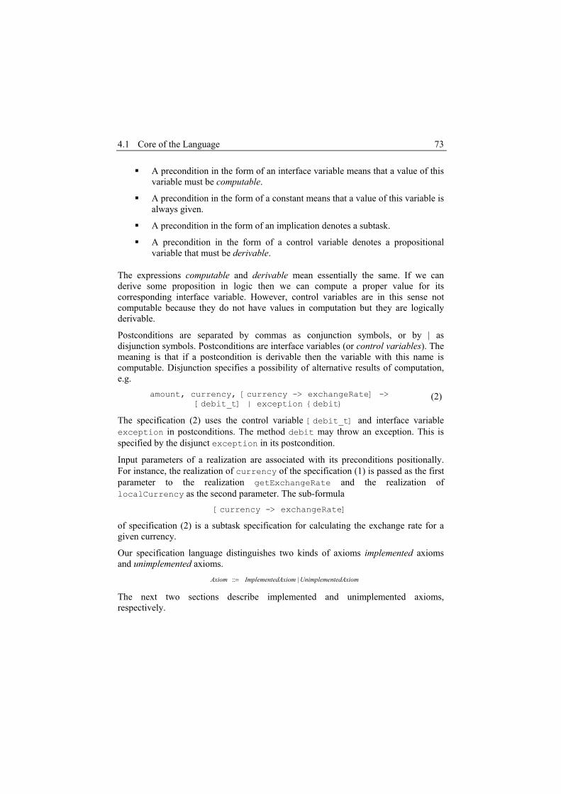
4.1 Core of the Language 73
A precondition in the form of an interface variable means that a value of this variable must be computable.
A precondition in the form of a constant means that a value of this variable is always given.
A precondition in the form of an implication denotes a subtask.
A precondition in the form of a control variable denotes a propositional variable that must be derivable.
The expressions computable and derivable mean essentially the same. If we can derive some proposition in logic then we can compute a proper value for its corresponding interface variable. However, control variables are in this sense not computable because they do not have values in computation but they are logically derivable.
Postconditions are separated by commas as conjunction symbols, or by | as disjunction symbols. Postconditions are interface variables (or control variables). The meaning is that if a postcondition is derivable then the variable with this name is computable. Disjunction specifies a possibility of alternative results of computation, e.g.
amount, currency, [currency -> exchangeRate] -> [debit_t] | exception {debit}
(2)
The specification (2) uses the control variable [debit_t] and interface variable exception in postconditions. The method debit may throw an exception. This is specified by the disjunct exception in its postcondition.
Input parameters of a realization are associated with its preconditions positionally. For instance, the realization of currency of the specification (1) is passed as the first parameter to the realization getExchangeRate and the realization of localCurrency as the second parameter. The sub-formula
[currency -> exchangeRate]
of specification (2) is a subtask specification for calculating the exchange rate for a given currency.
Our specification language distinguishes two kinds of axioms implemented axioms and unimplemented axioms.
:: |Axiom ImplementedAxiom UnimplementedAxiom=
The next two sections describe implemented and unimplemented axioms, respectively.

Chapter 4 Specification Language 74
4.1.5 Implemented Axioms A specification of an implemented axiom is a declaration of the form
:: [ [', ' ]] ' ' ( [' | ' ]) | '{' '}'
| ' ' ( [' | ' ]) | ' ' '{' '}'
::
ImplementedAxiom IdentifierList SubtaskList Identifier Alternatives falsity Realization
SubtaskList Identifier Alternatives falsity Realization
IdentifierList Id
= − >
− >
= [', ' ]
:: [' | ' ]
:: [', ' ]
entifier IdentifierList
Alternatives Identifier Alternatives
SubtaskList Subtask SubtaskList
=
=
The declaration of an ImplementedAxiom asserts that its specification is realized by Realization (which denotes a pre-programmed module), where IdentifierList is a possibly empty list of names of declared interface variables, and SubtaskList is a possibly empty list of subtask specifications. Objects identified by these two lists act as input parameters of the realization of the axiom and Identifier, Alternatives, or falsity act as output parameter, where falsity is a constant. In case the list Alternatives is not empty, the realization of the axiom may have an alternative outcome, where the realization of the axiom shows explicitly which output parameter has been computed.
Example. For instance, assuming some component with two realizations getExchangeRate and getLocalCurrency for calculating the exchange rate of a given currency and the local currency, we can introduce interface variables currency for a source currency, localCurrency, and exchangeRate, for the local currency and exchange rate, respectively, and declare an axiom that specifies how we can calculate the exchange rate. We extend the metainterface Exchange of section 4.1.1 with two specifications of computability as follows:
currency, localCurrency -> exchangeRate {getExchangeRate} -> localCurrency {getLocalCurrency}
The metainterface Exchange extended with specification of computability then looks as follows:
Exchange { currency :: String, localCurrency :: String, exchangeRate :: float, currency, localCurrency -> exchangeRate {getExchangeRate}, -> localCurrency {getLocalCurrency} }

4.1 Core of the Language 75
4.1.6 Unimplemented Axioms A specification of an unimplemented axiom is a declaration of the form
:: [ ] ' ' '{ }'UnimplementedAxiom IdentifierList Identifier spec= − > ,
where IdentifierList is a possibly empty list of names of interface variables and constants and Identifier is the name of an interface variable. The keyword spec specifies that this specification is an unimplemented axiom.
In contrast to implemented axioms, specifications of unimplemented axioms cannot have specifications of subtasks and alternative outcomes. Subtasks are branches and alternative outcomes result in branching, i.e., subtasks. We can namely synthesize the subtasks but we have no information about how to deploy the synthesized subtasks in a realization of an unimplemented axiom.
A specification of an unimplemented axiom does not state any realizability. It states only that, for any composed program, interface variables and constants occurring in IdentifierList act as input parameters and Identifier is the output parameter of the unimplemented axiom. Whenever this axioms is used in the composition of a program, the realization of this axiom has to be synthesized.
Example. Reconsider the metainterface ExchangeRate of section 4.1.3. We can add the unimplemented axiom
currency -> exchangeRate {spec}
to this metainterface; this gives a program for computing the exchangeRate of a given currency and the local currency as follows:
ExchangeRate { currency :: String, exchangeRate :: float, exch :: Exchange, exch = (Exchange), exch.currency = currency, exch.exchangeRate = exchangeRate, currency -> exchangeRate {spec} }
A realization for computing the exchangeRate of a given currency and the local currency is synthesized if it is needed.
4.1.7 Subtasks Axioms may contain specifications of functional parameters, which we call subtasks. A subtask behaves like an ordinary input parameter, but it behaves also like a goal. In this sense a subtask is an unimplemented axiom whose realization must be composed

Chapter 4 Specification Language 76
according to the specification; however, it can be invoked only by the realization of the axiom where the subtask occurs.
We distinguish two kinds of subtasks: dependent and independent subtasks. For subtasks we add the following expression to our language definition:
:: |Subtask DependentSubtask IndependentSubtask=
The next two subsections explain dependent and independent subtasks, respectively.
4.1.8 Dependent Subtasks Dependent subtasks may occur in axioms as preconditions. A precondition in the form of an implication is a dependent subtask which denotes a subgoal to compute values for the interface variable on its right-hand side from given values of the interface variables on its left-hand side and values of interface variables computed before (therefore it is dependent). The realization of a subtask is a synthesized program.
A dependent subtask has the form:
:: '[' [ ] ' ' '] 'DependentSubtask IdentifierList Identifier= − > ,
where Identifier is the name of a declared interface variable and denotes the output of the subtask, and IdentifierList is a possibly empty list of names of interface variables and denotes the input of the subtask.
For any composed program, the realization of an axiom cannot be invoked if some subtask of the axiom does not have a realization. The realization of a subtask is a program that acts as input for the realization of the axiom.
4.1.9 Independent Subtasks Independent subtasks may also occur in axioms as preconditions. A precondition in the form of an implication preceded by a MetaInterfaceName is an independent subtask which denotes a subgoal to compute values for the interface variable on its right-hand side from given values of the interface variables on its left-hand side using only the given metainterface (denoted by MetaInterfaceName) as a specification (therefore it is independent). The realization of an independent subtask is also a synthesized program.
An independent subtask has the form
:: '[' ' | ' [ ] ' ' '] 'IndependentSubtask MetaInterfaceName IdentifierList Identifier= − − > ,
where Identifier is the name of an interface variable of the metainterface identified by MetaInterfaceName, it is the output of the subtask, and IdentifierList is a possibly empty list of names of interface variables of the same metainterface and denotes the input of the subtask.

4.2 Language Extensions 77
Similar to the case of dependent subtasks, the realization of an axiom cannot be invoked if some independent subtask of the axiom does not have a realization. The realization of a subtask is a program that acts as input for the realization of the axiom.
4.1.10 Goals A goal specifies a program to be composed. To specify goals we use a sequent notation. The form of goal is the following:
:: ' | ' [ ] ' ' [ '. ']
:: [', ' ]
:: [ '. '] [', ' ]
Goal MetaInterfaceList Assumptions MetaInterfaceName Identifier
MetaInterfaceList MetaInterfaceName MetaInterfaceList
Assumptions MetaInterfaceName Identifier Assumptions
= − − >
=
=
The antecedent MetaInterfaceList of the sequent is a list of names of metainterfaces of components and the consequent of the sequent is a formula that specifies the program to be composed. Assumptions is a list of input parameters and MetaInterfaceName.Identifier is the output parameter of the program to be composed. Prefixes MetaInterfaceName occurring in assumptions are names of metainterfaces, which must occur in the list of names of metainterfaces. Suffixes Identifier are identifiers of interface variables of their respective metainterfaces. The list MetaInterfaceList of names of metainterfaces may be not complete, i.e. may not necessarily contain all metainterfaces that are needed for composing the program specified by [ ] . Otherwise, if we demanded this list to be complete, it would be required to know in advance all needed metainterfaces that are involved in composition of the requested program.
' ' [ '. ']Assumtions MetaInterfaceName Identifier− >
Example. Reconsider the metainterface ExchangeRate of section 4.1.3. It can be used for several purposes. The actual usage will be determined by a goal. For instance, the goal: ExchangeRate|-ExchangeRate.currency->ExchangeRate.exchangeRate
gives a program for computing the exchangeRate of a given currency and the local currency.
4.2 Language Extensions
Here we consider two extensions to the core language. The first one concerns first-order features and required extending the logic of axioms by metavariables; the second extension is the introduction of control variables. Control variables can be translated into the logic of the core language.

Chapter 4 Specification Language 78
4.2.1 Metavariables Specifiers of interface variables and constants may be names of metainterfaces. In this way we can build aggregation hierarchies and link metainterfaces explicitly. We call those hierarchies also static configurations. We explicitly link interface variables and constants of metainterfaces occurring (names of metainterfaces are used as specifier of interface variables or constants) in static configuration through bindings. So, using interface variables and constants we predefine the usage of a certain metainterface within a static configuration and specify explicitly how a particular interface variable can get a realization.
Example. Let us reconsider the metainterface ExchangeRate, which we have already used in section 4.1.3.
ExchangeRate { currency :: String, exchangeRate :: float, exch :: Exchange, exch = (Exchange), exch.currency = currency, exch.exchangeRate = exchangeRate }
The specifier of the interface variable exch denotes the metainterface Exchange. The two bindings:
exch.currency = currency and exch.exchangeRate = exchangeRate
predefine the role of Exchange within the static configuration built by ExchangeRate. They denote that realizations of currency and exch.currency must have equal values and realizations of exchangeRate and exch.exchangeRate must have equal values.
Using only interface variables and constants forces us to predefine any usage of a metainterface, which leads to static configurations that prevent automated selection of suitable metainterfaces at composition time, which in turn limits flexibility. On the contrary, the binding exch=(Exchange) specifies that any instance of Exchange, which is specified by the metavariable (Exchange), is an appropriate value for exch, but how to compute that instance is not specified and must be found by synthesis.
Metavariables may appear in bindings and axioms. The specification of a metavariable has the form:
:: '(' ') 'Metavariable ComponentName= .
Operationally, a metavariable specifies that a composed program may involve an object o in computations, which is an instance of the named component. ComponentName does not refer to any declared interface variable; it is a name of an

4.2 Language Extensions 79
existing component, or possibly of a metainterface. Logically, a metavariable is a unary predicate with the intended meaning: “o is instance of the component identified by ComponentName”.
A metavariable (Q) as a precondition is satisfied if an object o satisfying the predicate “o is instance of component Q” is found. A metavariable as a postcondition denotes that an object o satisfying the predicate “o is instance of component Q” will be computed.
Accordingly, we extend the binding, dependent and independent subtask, and axiom expressions of our language definition as follows:
:: |
:: [', ' ]
:: [' | ' ]
:: ' '
:: '[' [ ] ' '
Parameter Identifier Metavariable
ParameterList Parameter ParameterList
Alternatives Parameter Alternatives
Binding Parameter Parameter
DependentSubtask ParameterList Parameter
=
=
=
= =
= − > '] '
:: '[' ' | ' [ ] ' ' '] '
:: [ [', ' ]] ' ' ( [' | ' ]) | '{' '}'
| '
IndependentSubtask MetaInterfaceName ParameterList Parameter
ImplementedAxiom ParameterList SubtaskList Parameter Alternatives falsity Realization
SubtaskList
= − − >
= − >
− ' ( [' | ' ]) | '{' '}'
:: [ ] ' ' '{ }'
Parameter Alternatives falsity Realization
UnimplementedAxiom ParameterList Parameter spec
>
= − >
Example. We can use metavariables instead of interface variable to specify that exception handling must b e provided by some other metainterface, e.g.
no -> (Account) | (Exception) {getAccount} (3) amount, currency, [currency -> exchangeRate]->
[debit_t] | (Exception) {debit} (4)
The second disjunct of both specifications is the metavariable (Exception). The formula that specifies the realization debit is the same as we used before in section 4.1.4, but the interface variable exception has been replaced with the metavariable (Exception). Both specifications state that exception handling must be provided by some other metainterface, which is detected automatically during synthesis if a suitable metainterface for exception handling exists. The difference between the specification we used in section 4.1.4 and (4) is that we in (3) and (4) do not predefine explicitly how exception handling should be carried out. Any component that can handle exceptions (i.e., a component that provides a realization that takes as input instances of component Exception) can takeover exception handling. For example, one can use the following metainterface of the component ExceptionHandler for handling exceptions:

Chapter 4 Specification Language 80
ExceptionHandler { ->(ExceptionHandler) {ExceptionHandler}, (Exception) -> falsity {handleException},}
This metainterface provides a realization that takes as input any object that is an Exception. The falsity constant in the postcondition of the specification of realization handleException specifies that after execution of handleException any other program instruction is valid.
Example. If we wish to specify that the local currency (see example of section 4.1.5) can be found from an object LocalCurrency, we can use a metavariable (LocalCurrency) and replace the specification:
-> localCurrency {getLocalCurrency}
by (LocalCurrency) = localCurrency {id}
This extension enables us to detect automatically a local currency that may depend on the location where the service will be used, if it is specified in some accessible metainterface.
Within a metainterface definition we can use the same identifier for the metainterface name, for a metavariable, as specifier of an interface variable, and for a realization. Let us extend the metainterface Exchange with the axiom:
-> (Exchange) {Exchange}
The metainterface Exchange extended with this specification of computability is the following:
Exchange { currency :: String, localCurrency :: String, exchangeRate :: float, -> (Exchange) {Exchange}, currency, localCurrency -> exchangeRate {getExchangeRate}, -> localCurrency {getLocalCurrency} }
The name Exchange now occurs as interface name, as metavariable name, and as realization. The realization {Exchange} is used here as a constructor for an instance of the component (Exchange).
The following rules (which are exclusive) apply for giving meaning to metavariables, interface variables, constants, and realizations:
4.2 Language Extensions 81
If the metainterface name is the same as the specifier of an interface variable or constant, then the specifier denotes the type of the interface variable or constant, respectively.
If the metainterface name is the same as the name of a metavariable, then an instance of the corresponding component of the metainterface is meant.
If the metainterface name is the same as the realization of a module, then the corresponding component’s constructor is meant.
4.2.2 Control Variables An axiom is used to determine when its realization can be applied and what it computes. We may want to control the usage of a realization in order to force its application only if additional conditions are met. We can use additional pre- and post conditions that do not have any values associated during computations. They are used only to guide the synthesis process to find the intended position of a realization’s application in a certain context. We call those pre- and postconditions control variables. Control variables may appear in bindings, subtasks, and axioms. Therefore we provide a new element for the syntactic domains Binding, DependentSubtask and IndependentSubtask, and Axiom.
The specification of a control variable has the form
:: '[' '] 'ControlVariable Identifier= ,
where Identifier refers to the name of the control variable being declared. A control variable does not refer to any interface variable.
Operationally, a precondition in the form of a control variable in square brackets does not have any computational meaning, but must be derivable when the axiom is used in a proof. Logically, a control variable is a propositional variable.
We require control variables occurring in the input parameter list of a realization to lead this list, and control variables of the output parameter list to finish this list. Accordingly, we extend our language definition as follows:

Chapter 4 Specification Language 82
:: [', ' ]
:: [ ', ']
:: [', ' ]
::
ControlVariableList ControlVariable ControlVariableList
InputParameterList ControlVariableList ParameterList
OutputParameter Parameter ControlVariableList
Alternatives OutputParameter
=
=
=
= [' | ' ]
:: '[' [ ] ' ' | '] '
:: '[' ' | ' [ ] ' ' | '] '
Alternatives
DependentSubtask InputParameterList Parameter ControlVariable
IndependentSubtask MetaInterfaceName InputParameterList Parameter ControlVariable
ImplementedA
= − >
= − − >
:: [ [', ' ]] ' '
( [' | ' ]) | '{' '}'
| ' ' ( [' | ' ]) | '{' '}'
:
xiom InputParameterList SubtaskList
OutputParameter Alternatives falsity Realization
SubtaskList OutputParameter Alternatives falsity Realization
UnimplementedAxiom
= − >
− >
: [ ] ' ' | '{ }'InputParameterList OutputParameter ControlVariableList spec= − >
4.3 Logical Semantics
Initially we implemented the same semantics of specifications that was used in the PRIZ and NUT systems (Mints 1991, Mints and Tyugu 1982). We were thus able to use the structural synthesis of programs as described already in (Tyugu 1994). This guaranteed good scalability and good performance of the synthesis. However, the logic of SSP was too restricted for expressing some important properties of service programs, first of all throwing exceptions. Moreover, context-awareness (which is an important feature of the synthesis of services) required another extension, the introduction of predicates that describe the appropriateness of some computable objects for binding independently developed components. Here we will describe the translation of the constructs of the specification language into our logical language.
4.3.1 Unfolding Unfolding is used for representing the semantics of interface variables and constants whose specifier is given by a metainterface. Reconsider the metainterface ExchangeRate described above.
ExchangeRate { currency :: String, exchangeRate :: float, exch :: Exchange, exch = (Exchange), exch.currency = currency, exch.exchangeRate = exchangeRate }
Its logical semantics is expressed by a collection of formulae. If a new interface variable exchR::ExchangeRate is specified (as it is in the metainterface Account shown below), then the formulae of ExchangeRate are explicitly inserted into the

4.3 Logical Semantics 83
logical specification and the prefix exchR is added to all names (except names of metavariables) in these formulae. This leads to expansion of the specification, but avoids excessive usage of universal quantifiers. It flattens all specifications of all metainterfaces.
Example. Consider the metainterface Account: Account { amount :: int, currency :: String, exchangeRate :: float, exch :: Exchange, exch = (Exchange), exch.localCurrency = currency, exchR :: ExchangeRate, exchR = (ExchangeRate), exchR.currency = currency, exchR.exchangeRate = exchangeRate, amount,currency, [currency->exchangeRate]->[debit_t]|(Exception) {debit} }
The metainterface Account we have presented here provides a transaction debit to debit an account. Its metainterface declares five interface variables: amount, currency, exchangeRate, exch, and exchR. The interface variables exch is used only to compute the local currency. We use the control variable [debit_t] to specify the final state of a complete transaction that involves the realization debit and exception handling. Let us use Account to illustrate the change in specifications if we unfold this metainterface. The first prefix to be added to all names of interface variables, constants and control variables (excluding metavariables) is the name of the metainterface, which is Account. For instance, all occurrences of the identifier of the interface variable amount become Account.amount. The axiom specifying the realization debit is replaced by:
Account.amount,Account.currency, [Account.currency->Account.exchangeRate]->
[Account.debit_t] | (Exception)
Metavariables are left unchanged, e.g., (Exception) remains as it is. The unfolding is done hierarchically, if required.
4.3.2 Structural Properties Structural properties of objects are represented computationally in our logic. We avoid the usage of description logic (Devanbu and Jones 1994) for representing structures, although it has been designed for this purpose. In this way we keep the

Chapter 4 Specification Language 84
control over proof search and preserve its high performance. The semantics of a structure ( )1, , kX x x= … , in particular, of a metainterface X having interface variables
1, , kx x… is expressed computationally by the axioms 1, , kX x x⊃ … and 1, , kx x X⊃… where identifiers denote the computability of variables with the same names. (This conforms to our usage of variables names in axioms, which we have described above.) These formulae express that the structural value is computable when all its components are given, and, vice versa, all its components are computable when the structured value itself is known. We have to take into account the structures when equalities are present. In the case of equality of two structures, e.g.,
( ):: , ::x y x= X y X , we have to be able to infer the computability of any of the components of any of them as soon as a respective component of the other is given. An easy way to guarantee this property in our logic is to unfold the equality explicitly for all components, i.e. to write automatically . .x z y z= for all components z of x and y.
4.3.3 Instance Value Instance value is a special concept needed for distinguishing an instance of a component from a structure composed from realizations of all its interface variables. In the translation from specification into the logical language we write x to denote that a value computed for the interface variable x is an instance of the component of x, but not the structure constructed from its interface variables. This distinction is essential in object-oriented computing.
4.3.4 Logical Semantics of Metainterfaces We now give logical semantics of expressions of our specification language. This logical semantics is given by translating specifications into the logical language LL1 of ESSP in a straightforward way.
A metainterface is a specification of a component. It consists of specification expressions sexp of our specification language described above. We use MI to range over names of metainterfaces. The auxiliary function sp is needed to generate a set of specification expressions of the metainterface denoted by a given metainterface name. Furthermore we use:
τ To denote the set of valid types of the target programming language, C To range over names of components, S To range over specifiers of interface variables and constants, o To range over object-prefixes, a,b To range over well-formed syntactic constructs of the specification language,
where their particular syntax depends on the context in which they occur, e.g. they may be simply a name, a compound name, a subtask specification, an admissible left- or right-hand side of the main implication of an axiom, etc.,

4.3 Logical Semantics 85
v To range over identifiers of interface variables and constants, r To range over realizations of interface variables and constants, val To range over constants of the target programming language, m To range over names of modules, which are realizations of axioms, id To denote the identity function, this function is overloaded, it suits to the
needed type.
Object-prefix is a concept that allows us to flatten specifications without loss of information. An object-prefix is a compound name, e.g. x.y. Such a compound name is constructed as follows. If we need to unfold a metainterface, which is denoted by the specifier MI of an interface variable or constant , then we append the identifier v to the current object-prefix x.y and use the new compound name x.y.v as object-prefix to unfold the metainterface denoted by MI. While translating specification expressions into the logical language we prefix the current object-prefix of every interface variable and constant, and control variable occurring in specification expressions. This technique gives every interface variable, constant and control variable a unique identifier within a flattened specification.
::v MI :: { }v MI val
Unfolding as described above is applied to metainterfaces. We use the function unfold that applies the semantic function p ⋅L to each specification expression sexp of the metainterface of a given metainterface name. unfold is a function of a metainterface name producing a set of logical formulae. The semantic function invokes unfolding in case the specifier of an interface variable or constant denotes a metainterface. The function unfold is overloaded. The first variant receives one parameter, which is the name MI of the metainterface to unfold. It is used to unfold initially every available metainterface. The second variant, which is called only by
, receives two parameters, the name MI of the metainterface to unfold and an object-prefix o. A dot • denotes an empty object-prefix. The function unfold is defined as follows:
p ⋅L
p ⋅L
( ) ( ) ( ) ( ){ }( ) ( ) ( ){ }
::
, |
p p
p
unfold MI mi MI mi MI
unfold MI o sexp o sexp sp MI
= ∪ =
= ∈
i iL L
L
We invoke unfold for every metainterface and (MI ) ( ),MI ounfold is invoked by the
semantic function to map each specification expression sexp of a given metainterface MI to our logical language. Initially we invoke
pL ⋅
( )unfold for every metainterface MI. This introduces for every metainterface MI an additional fresh interface variable mi whose specifier is MI. It also introduces an additional binding
that is needed to specify how to compute a proper value for mi, i.e. if there is either some constructor or some other module that can supply an instance of the corresponding component of the metainterface MI.
MI
(mi MI= )

Chapter 4 Specification Language 86
Example. As a running example we present here unfolding of the metainterface ExceptionHandler. For convenience we show this metainterface again.
ExceptionHandler { ->(ExceptionHandler) {ExceptionHandler}, (Exception) -> falsity {handleException},}
After unfolding ( ( )unfold ExceptionHandler ) we obtain the following specification in our logical language: r : ExceptionHandler id : ∀x.ExceptionHandler(x) ⊃ ExceptionHandler id : ExceptionHandler ⊃ ∃w.ExceptionHandler(w) ExceptionHandler : 2 ⊃ ∃y.ExceptionHandler(y) (r, handleException) : ExceptionHandler ∧ ∀z.Exception(z) ⊃ ⊥
The first line introduces an object variable (see section 3.2.1). The second and third lines are results of the introduced binding. The forth and fifth line are the results of translation of the constructor ExceptionHandler and module handleException respectively.
Interface variables of a metainterface are translated into object variables (see section 3.2.4) in the following two ways, depending on its specifier. Let o be the current object-prefix. First, if the specifier of the interface variable denotes a type of the underlying programming language, then an interface variable is mapped to an object variable , where r denotes the realization (object) of o.v, S denotes its type, and the symbol ‘:’ denotes realization. Second, the specifier of the interface variable denotes a name
::v S: .Sr o v
'MI
'
of another metainterface. Then, the interface variable is mapped to an object variable of the form r , where r denotes the
realization of o.v and :: 'v MI ' : .MI o v
MI denotes its type, and additionally we unfold the metainterface denoted by 'MI through unfold( 'MI , ) and translate specification expressions of the metainterface denoted by
.o v'MI using the new prefix . .o v
Constants are treated as functions. They are translated into object variables and implications with empty premises. A constant of some metainterface and object-prefix o is translated into an unconditional computability statement
:: { }v S val: .val o v⊃2
Bindings are translated into two unconditional computability statements. A binding of some metainterface is rewritten into two specifications a ba b= { }id− > and
on which we apply the translation { }idb a− > p ⋅L .
Axioms written in a specification are translated into logic in a straightforward way. They are implications with preconditions on the left and postconditions on the right side. A realization may have an alternative outcome (throwing an exception for

4.3 Logical Semantics 87
instance), which is specified by an implication with disjunction on its right side. A realization m (module) of an axiom is invoked on realizations (objects) of its variables. In order to avoid unnecessary introduction of quantifiers we make use of our unfolding strategy. In particular, we use the current object-prefix o to identify the object on which the realization m of the axiom must be invoked. An axiom
of a metainterface is translated into the conditional or unconditional
computability statement , where o is the current
object-prefix, and is the realization of that object variable which is identified by the object-prefix o. It is the realization on which the module m must be applied. The extra precondition o in the formula is needed to force the derivation of o prior derivation of b, i.e. application of m. If m identifies a constructor or m it is the keyword spec then we simply have m a
{ }a b m− >
( ) ( )( , ) :o l rSr m o a o b o∧ ⊃L L
( )lo a o∧ ⊃L L
:
oSr
( )r b
b
o
⊃ , because constructors are not invoked on instances of the respective component and spec is not a defined realization of any component.
Metavariables are translated into the logic with quantifiers: as a universal quantifier among the preconditions and an existential quantifier among the postconditions. Examples are as follows: Let m be a module of some component, then
gives
( ), { }C a b m− >
( , ) : . ( )oSr m w C w a b∀ ∧ ⊃ and ,( ) { }a b C m− > gives ( , ,
where a and b need still to be translated. )o
Sr m : . ( )a b w C w⊃ ∧ ∃
Control variables are simply propositional variables, e.g., a control variable [a] occurring in some specification expression of a metainterface is translated into o.a, where o is the current object-prefix.
Definition (Semantic of specifications)
Let SExp be the set of valid specification expressions, O be the set of compound names (object-prefixes), and let LL1 represent the set of all valid formula of our logical language. A compound name with a leading dot of the form is simply identified with n. Logical semantics of expressions of specifications are determined by the function
.ni
( ): 1p SExp LL⋅ → →L O ,
which is a mapping from expressions of specifications to our logical language LL1 that we have described in section 3.3.3. The logical semantic function is given by:

Chapter 4 Specification Language 88
( )
( ) ( ) ( )( ) ( )
( )( )( ) ( )
: .:: : . ( , . ):: { } :: { }
. ( ). ( )
.[ ]
p SS
p p p
p
p
p
p p
p
r o v if Sv S o r o v unfold S o v otherwisev S val o v S o v val o
w C w if p lC o w C w if p rfalsity o
b o o b where b is a namea o a o
a
τ∈= ∪= ∪ − >
∀ == ∃ == ⊥
=
=
L
L L L
L
L
L
L L
L ( ) ( ) ( )( ) ( )( ) ( )( ) ( )( ) ( ) ( )
{ } ( ) ( ){ } ( )
{ } { }
|
p p
p p
p p
p r
p l r
p p
p
b o a b id o b a id oa b o a b o
MI a b o a b MI
a o a oa b o a o b o
a b spec o a b o
a b val o va
= = − > ∪ − >
− > = − > − − > = − >
− > = ⊃
− > = ⊃
− > = − >
− > =
2
L L
L L
L L
L L
L L L
L L
L ( ){ } ( ) ( )
{ } ( )( )
( ) ( )( ) ( ) ( )( ) ( ) ( )
:
:
:
, :
,|
p
p p
pp
o pS
p p p
p p p
l a b o
a b id o id a b o
m a b o if m is constructor ora b m o
r m o a b o otherwise
a b o a o b oa b o a o b o
− >
− > = − >
− >− > = ∧ − >
= ∧
= ∨
spec
L
L L
LL
L
L L L
L L L
The logical interpretation of metavariables depends on the context in that they occur. The extra parameter p of specifies this context. p ⋅L

Chap t e r 5
Synthesis
In this chapter we describe our method for developing a service program to realize a given service specification. We continue the example that we have introduced in Chapter 4.
5.1 General Scheme of Synthesis
Let Q be a list of metainterfaces and M1, M2 metainterfaces, where x, y represent an interface variable, metavariable, or control variable of M1, M2 respectively. For simplicity we use M1.x instead of M1.x, which is a list or conjunction of names of interface variables. A service request is specified in our specification language as follows:
1. 2.Q M x M y⊃0
This service specification is interpreted as compute M2.y from M1.x when Q. It is then translated into a set of axioms T in our logical language LL1 in which the theorem ( )1. 2.T f M x M y∃ ⊃0 is constructively provable for each realizable service. If we have such a proof a service program, which satisfies the specification can be extracted from it. We illustrate the general scheme of synthesis in Figure 7.
89

Chapter 5 Synthesis 90
Specification language compute M2.y from M1.x when Q
( )1. 2.T f M x M y∃ ⊃0
Service program extraction
Fully automated deduction
Programming language Service program
proof
Logical language (LL1)
Translation
Figure 7 General scheme of service synthesis
As we can see in Figure 7, there are two specification levels. The first level comprises the source specifications Q that contains M1, M2, and all other known metainterfaces. These specifications are written in our specification language (see Chapter 4). On transition to the second level the source specification Q is translated into an extended specification in the form of a formal theory T, which is encoded in our logical language LL1. The formal theory T is used to prove the existence theorem for the given service. We emphasize that the translation from the source specification Q into the formal theory T (as describes in section 4.3) is an essential and important feature of our service synthesis approach. It involves unfolding of hierarchies of metainterfaces as well as generation of new axioms. The formal theory T is a flat representation of the source specification Q and allows efficient synthesis because we can avoid excessive use of quantifiers.
5.2 Synthesizing a Service Component
We are using the concept of meta-components in order to distinguish a component supplied with a metainterface from a conventional component. In our implementation we keep a specification of a component as a part of the component in the form of a string. This allows us to implement a meta-component as a regular component.

5.2 Synthesizing a Service Component 91
Our specification language has a straightforward translation into a restricted first-order constructive logic (see section 4.3). Axioms have a realization given by a pre-programmed module of the component to whose specification the construction belongs. In particular, an implication like ->localCurrency may have an implementation in the form of a module, e.g.,
String getLocalCurrency().
Then we denote this association in the specification by showing a name of the respective module in curly brackets, e.g.,
-> localCurrency {getLocalCurrency}.
Synthesizing a service component C proceeds as follows. One writes a specification (metainterface) of the new component, using existing meta-components and components, and also writes a top-level goal in the form of an implication P->R where P is precondition and R is postcondition of the module of the new service component to be synthesized. So, the goal is to find a realization for the implication P->R in the form of a new module of the new component C. This is achieved by our general schema of deductive program synthesis: derive P->R using logical formulae of specifications as specific axioms, and extract the realization of the goal from its derivation. The realization of the goal is executed in a new module of the component C. New subgoals may appear during this derivation, hence, more modules of the component C may be synthesized completely automatically. Moreover, attributes of the new component may be introduced. In particular, any proposition with the meaning “the interface variable x has a correct value” may get a realization as an attribute of the new component.
Example. As an example we present here the synthesis of a component ExchangeRate from the metainterface ExchangeRate, which we have already discussed in section 4.1.6 but repeat it here:
ExchangeRate { currency :: String, exchangeRate :: float, exch :: Exchange, exch = (Exchange), exch.currency = currency, exch.exchangeRate = exchangeRate, currency -> exchangeRate {spec} }
This metainterface uses the meta-component Exchange. It declares an interface variable exch. We also have a declaration of an unimplemented axiom, which is specified by the keyword spec in the realization of the axiom. The last two bindings of this metainterface configure statically the intended usage of the meta-component Exchange within the metainterface ExchangeRate. In order to reuse the meta-

Chapter 5 Synthesis 92
component Exchange the user must know the metainterface Exchange, and in particular its intended usage.
The first step before synthesis of a new component is unfolding of all available metainterfaces. After unfolding ExchangeRate we obtain the following specification, where we avoid showing axioms introduced by structures. We also do not write the types of realizations of object variables. // Extra axioms r : ExchangeRate id : ∀x.ExchangeRate(x) ⊃ ExchangeRate id : ExchangeRate ⊃ ∃y.ExchangeRate(y)
// Interface variables o : ExchangeRate.currency p : ExchangeRate.exchangeRate q : ExchangeRate.exch
// Binding: exch = (Exchange) id : ∀z.Exchange(z) ⊃ ExchangeRate.exch id : ExchangeRate.exch ⊃ ∃w.Exchange(w)
// Binding: exch.currency = currency id : ExchangeRate.exch.currency ⊃ ExchangeRate.currency id : ExchangeRate.currency ⊃ ExchangeRate.exch.currency
// Binding: exch.exchangeRate = exchangeRate id : ExchangeRate.exch.exchangeRate ⊃ ExchangeRate.exchangeRate id : ExchangeRate.exchangeRate ⊃ ExchangeRate.exch.exchangeRate
// Unimplemented axiom: currency -> exchangeRate {spec} spec : ExchangeRate.currency ⊃ ExchangeRate.exchangeRate // Unfolded Exchange of: exch : Exchange
// Interface variables oo : ExchangeRate.exch.currency t : ExchangeRate.exch.localCurrency pp : ExchangeRate.exch.exchangeRate
// Axioms (q,getExchangeRate) : ExchangeRate.exch ∧ ExchangeRate.exch.currency ∧ ExchangeRate.exch.localCurrency ⊃ ExchangeRate.exch.exchangeRate
(q,getLocalCurrency) : ExchangeRate.exch ⊃ ExchangeRate.exch.localCurrency
Exchange : 2 ⊃ ∃u.Exchange(u)

5.2 Synthesizing a Service Component 93
Unfolding a metainterface starts with introducing an additional interface variable and binding (see section 4.3.4, Unfolding). For this particular example we translate first the additional interface variable ExchangeRate::ExchangeRate and thereafter we translate the additional binding ExchangeRate=(ExchangeRate). Translation of the interface variable ExchangeRate results in the object variable r:ExchangeRate where ExchangeRate is a propositional variable and r is an arbitrary but new name for the corresponding object. Since the specifier of the interface variable ExchangeRate denotes a metainterface, namely ExchangeRate, we unfold now this metainterface with the object prefix ExchangeRate, which is the identifier of the interface variable. Unfolding the metainterface ExchangeRate translates all specification expressions occurring in ExchangeRate into our logical language. Take for instance the interface variable exch. This interface variable is translated into the object variable q:ExchangeRate.exch where ExchangeRate.exch is a propositional variable and q is an arbitrary but new name for the corresponding object. The object-prefix ExchangeRate has been added to the identifier exch.
The metainterface Exchange is unfolded two times. First, because all known metainterfaces are unfolded separately before any synthesis takes place. Second, because the specifier of the interface variable exch of the metainterface ExchangeRate denotes the metainterface Exchange. The result of this translation is not shown above. For this particular example we would need only the latter translation. However, both translations of Exchange give beside other computability statements the following, which has been derived from ->(Exchange){Exchange}:
Exchange : 2 ⊃ ∃u.Exchange(u) (*)
The binding exch=(Exchange) implicitly specifies how to compute a value for the interface variable exch. In other words, since there is no axiom in the metainterface ExchangeRate that specifies explicitly how to compute a value for exch; any instance of the component Exchange is a suitable value. The translation of this binding gives two computability statements:
id : ∀z.Exchange(z) ⊃ ExchangeRate.exch id : ExchangeRate.exch ⊃ ∃w.Exchange(w)
The first of these two computability statements and (*) enables us to find a realization for the object variable q:ExchangeRate.exch.
Realizations of the meta-component Exchange must be invoked on an instance of the meta-component Exchange. But which instance? The instance is determined by the object-variable q:ExchangeRate.exch. Realizations of Exchange will be invoked on the object q, if we can find a realization for q, i.e., how to compute an instance of the meta-component Exchange. For the realizations getExchangeRate and getLocalCurrency of the meta-component Exchange for instance, the translation records this information in (q,getExchangeRate) and (q,getLocalCurrency), respectively.

Chapter 5 Synthesis 94
The second step is to write the top-level goal: ExchangeRate |- currency -> exchangeRate
This goal specifies that a program that computes the exchange rate for a given currency should be synthesized. The interface variable names currency and exchangeRate of this synthesis problem (i.e. sequent) do not have prefixes telling to which metainterface they belong. This is not needed here because the antecedent of the sequent contains only one metainterface, so no ambiguity may occur.
During synthesis the specification of the unimplemented axiom currency -> exchangeRate{spec}
is used, which causes the system to issue a new goal. The new goal is: |- currency -> exchangeRate
The consequent of this goal is the same as in our initial goal, but both goals are indeed different. The realization of |-currency->exchangeRate, if possible to derive, will yield an implementation spec_1 for the unimplemented axiom, whereas the realization of our initial goal yields a realization of a new module (program) with some arbitrary name m.
This second goal is derivable and hence our initial goal is derivable as well. Synthesis will detect that the metainterface ExchangeRate has no corresponding component. Therefore a new component ExchangeRate will be generated. The metainterface of this new component is the following:
ExchangeRate { currency :: String, exchangeRate :: float, currency -> exchangeRate {m} -> (ExchangeRate) {ExchangeRate} }
Observe that the declaration of the unimplemented axiom, bindings, and the interface variable exch have disappeared in the new metainterface and the realization of the initial goal became an implemented axiom. The realization spec_1 of the unimplemented axiom is now part of the implementation of our initial goal, i.e. the new module m simply invokes the realization spec_1, which is hidden now. The synthesis process of the module m is presented in Figure 8 as a “pseudo-proof”, where we show the stepwise application of unfolded specifications in parallel with the program schema of the service program being synthesized. By “pseudo-proof” we mean that it does not present the complete and exact proof tree generated by our logic, but rather a scheme of the actual proof; that is the witness of existence of a solution for the given problem (goal).

5.3 Synthesizing a Service 95
The realization of m and spec_1 is the following (pseudo-code): m (o) { p := spec_1 (o); return p; }
spec_1 (o) { q := Exchange(); t := q.getLocalCurrency(); p := q.getExchangeRate(o, t); return p; }
This pseudo-code is slightly optimised; we have removed unnecessary assignments that realize bindings. These realizations illustrate how interface variables, metavariables, and realizations of axioms are used by program extraction. Interface variables become local variables if they are not hypotheses and metavariables are replaced by module invocations.
Assume: o:ExchangeRate.currency
// proof new goal due to unimplemented axiom Assume: o:ExchangeRate.currency Exchange: 2 ⊃ ∃u.Exchange(u) Assume: Exchange(a) q: ExchangeRate.exch id: ∀z.Exchange(z) ⊃ ExchangeRate.exch oo: ExchangeRate.exch.currency id: ExchangeRate.currency ⊃ ExchangeRate.exch.currency t: ExchangeRate.exch.localCurrency (q,getLocalCurrency): ExchangeRate.exch ⊃ ExchangeRate.exch.localCurrency pp: ExchangeRate.exch.exchangeRate (q,getExchangeRate): ExchangeRate.exch ∧ ExchangeRate.exch.currency ∧ ExchangeRate.exch.localCurrency ⊃ ExchangeRate.exch.exchangeRate p: ExchangeRate.exchangeRate id: ExchangeRate.exch.exchangeRate ⊃ ExchangeRate.exchangeRate done! spec: ExchangeRate.currency ⊃ ExchangeRate.exchangeRate done!
Figure 8 Pseudo-proof to example exchange rate
5.3 Synthesizing a Service
Here we present synthesis of a service through an example. The example is synthesis of a transaction service, more precisely, debiting a bank account. The metainterfaces of meta-components needed for specifying this service are Bank, Naming, Account, Exchange, ExchangeRate, and ExceptionHandler. We have already specified these meta-components (see Chapter 4) except Bank and Naming. We assume here that all required (meta-)components are implemented in some programming language.

Chapter 5 Synthesis 96
The metainterfaces Bank and Naming are as follows: Bank { no :: long, url :: String, nm :: Naming, nm = (Naming), nm.url = url, (RemoteRef) = (Bank), no -> (Account) | (Exception) {getAccount} } Naming { url :: String, -> (Naming) {Naming}, url -> (RemoteRef) | (Exception) {lookup} }
The metainterface Bank we present here provides one module, which is getAccount to receive a reference to an account object that is identified by the account number no. The module lookup of the metainterface Naming is used to obtain a an object reference to a bank object that is associated with a given url (Uniform Resource Locator). This object reference is then used to obtain another object reference (by invoking the module getAccount on it) to an account object that is connected to a given account number no. Having access to an account object we can debit the corresponding account by invoking the module debit on the account object if we can solve the sub-problem to calculate the exchangeRate of the local currency and the currency of the location of the bank (see 4.3.1). Some modules of our metainterfaces may throw an exception, which is specified by using disjunction in the postconditions of the specifications of the respective modules. Due to disjunction, we have to solve additional sub-problems that take over the computation in case of exception.
It is our goal to derive a service program to debit an account at a bank. The input for this program is the url of a bank, the account number no, and the amount the respective account should be debited with. To synthesize this program we state the following goal:
Bank, Account |- Bank.url, Bank.no, Account.amount -> [Account.debit_t]
The list of metainterfaces (Bank, Account) of the antecedent of this goal does not contain all metainterfaces that are needed to synthesize our program. The synthesis also involves the metainterfaces Exchange, ExchangeRate, Naming, and ExceptionHandler. The deployment of the meta-component Account and ExceptionHandler is implicitly specified by the metavariables (Account) and

5.3 Synthesizing a Service 97
(Exception), while the deployment of the meta-component Exchange and ExchangeRate is explicitly specified in metainterfaces.
After unfolding of metainterfaces we obtain a flat representation of all specifications. The flat representation would fill at least four pages for this example. Therefore, we will show only specifications that we really need for composing our small service program. We will present the synthesis process again as pseudo-proof. The pseudo-proof is shown in Figure 9. In this pseudo-proof we use the label S for the sub-formula Account.currency⊃Account.exchangeRate, which has been derived from the subtask specification [currency->exchangeRate] (see section 4.1.7) of the specification of the realization debit of the meta-component Account. The proof of this subtask specification is presented separately but in the same figure.

Chapter 5 Synthesis 98
Assume: url:Bank.url, no:Bank.no, amount:Account.amount
Naming: 2 ⊃ ∃u.Naming(u) Assume: Naming(q) n:Bank.nm id:∀z.Naming(z) ⊃ Bank.nm id:Bank.url ⊃ Bank.nm.url (n,lookup): Bank.nm ∧ Bank.nm.url ⊃ ∃v.RemoteRef(v) ∨ ∃d.Exception(d)
Case: ∃d.Exception(d) see (*)
Case: ∃v.RemoteRef(v)
Assume: RemoteRef(f) id:∀x.RemoteRef(x) ⊃ ∃y.Bank(y) Assume: Bank(r) b:Bank id:∀a.Bank(a) ⊃ Bank (b,getAccount):Bank ∧ Bank.no ⊃ ∃c.Account(c) ∨ ∃e.Exception(e)
Case: ∃e.Exception(e) see (*)
Case: ∃c.Account(c)
Assume: Account(g) h:Account id:∀i.Account(i) ⊃ Account l:Account.exch Exchange: 2 ⊃ ∃m.Exchange(m) Assume: Exchange(o) id:∀p.Exchange(p) ⊃ Account.exch (l,getLocalCurrency):Account.exch ⊃ Account.exch.localCurrency s:Account.currency id:Account.exch.localCurrency ⊃ Account.currency (h,debit): Account ∧ Account.amount ∧ Account.currency ∧ S ⊃ Account.debit_t ∨ ∃k.Exception(k)
Case: ∃k.Exception(k) see (*)
Case: Account.debit_t done!
S: (Account.currency ⊃ Account.exchangeRate)
Assume: Account.currency ExchangeRate: 2 ⊃ ∃w.ExchangeRate(w) Assume: ExchangeRate(j) t: Account.exchR id: ∀x.ExchangeRate(x) ⊃ Account.exchR id: Account.currency ⊃ Account.exchR.currency (t,m): Account.exchR ∧ Account.exchR.currency ⊃ Account.exchR.exchangeRate id: Account.exchR.exchangeRate ⊃ Account.exchangeRate done!
(*)
Assume: Exception(e) exp:ExceptionHandler ExceptionHandler: 2 ⊃ ∃x.ExceptionHandler(x) Assume: ExceptionHandler(o) id: ∀y.ExceptionHandler(y) ⊃ ExceptionHandler (exp,handleException): ExceptionHandler ∧ ∀z.Exception(z) ⊃ ⊥ abort : Account.debit_t done!
Figure 9 Pseudo-proof to example bank

5.3 Synthesizing a Service 99
From this proof we can easily extract the desired service program, which is shown in Figure 10. The proof gives the program structure. Again, we present the extracted program in pseudo-code.
prog(url,no,amount) {
n := Naming(); tmp_1 := n.lookup(url);
switch(tmp_1) { case Exception: exp := ExceptionHandler(); exp.handleException(tmp_1); break;
case RemoteRef: b := tmp_1; tmp_2 := b.getAccount(no);
switch(tmp_2) { case Exception: exp := ExceptionHandler(); exp.handleException(tmp_2); break;
case Account: h := tmp_2; l := Exchange(); s := l.getLocalCurrency(); tmp_3 := h.debit(amount,s,subtask_1);
switch(tmp_3) { case Exception: exp := ExceptionHandler(); exp.handleException(tmp_3); break;
default: break; } break; } break; } }
subtask_1(s) {
t := ExchangeRate(); return(t.m(s)); }
Figure 10 Extracted program (pseudo-code)

Chapter 5 Synthesis 100
The example illustrates also how the usage of disjunction (i.e., modules throwing exceptions) introduces case statements. Our proof strategy of proving disjunction converts the specification of a module with disjunction into a module with subtasks (see section 3.3.6). The realizations of these modules are then inserted into the program, which are the blocks of case statements.

Chap t e r 6
Application to Java
6.1 Introduction
Early Java environments suffered from difficulties in the reuse of classes (first of all, related to GUI). As a remedy, JavaBeans were introduced. This was followed by the introduction of Enterprise Java Beans (EJB) as components of domain-oriented applications. In both cases, classes were supplied with additional information, and mechanisms (e.g. beanboxes) were developed for using this information. We introduce a similar extension of Java classes that will be supported by our domain-independent program synthesis technique. As this work has been performed in the context of the larger project Personal Computing and Communication (PCC) (PCC Workshop 2001), we have the practical goal to apply our technique to just-in-time synthesis of services from pre-programmed components. The synthesis method must be 1) efficient, because service program composition is performed in a dynamic environment at runtime, 2) autonomous, because the user has no abilities to provide help in the synthesis process, 3) it must guarantee the correct deployment of components, and 4) the service composition system must support a specification language that enables users to write specifications for synthesis in a reasonably easy way.
101

Chapter 6 Application to Java 102
We have chosen Java as the language we extend because it is a widely used object-oriented language suitable for implementing services in a network. Components of services are represented as classes and interfaces. Pre-programmed modules are methods and constructors of classes. Special attention is paid to handling exceptions in Java in a logically sound way. Also, handling constructors requires special attention.
The remainder of this chapter is organized as follows. We describe first how to supply classes with specifications using our specification language. Thereafter, extracting Java programs from proofs will be explained. Then we describe Java program synthesis and conclude this chapter with experimental results with respect to synthesis performance.
6.2 Adding Specifications to Classes
Java is an object-oriented programming language. The application of our specification language to Java combines object-oriented programming with logic programming: after extending Java classes with a declarative part, fully automated composition of Java programs from structural specifications is possible (Lämmermann 2000). This combination has also been tried out in the NUT system (Tyugu 1994). Uustalu reported in (Uustalu 1995b) the logical semantics of the declarative part of the NUT language. Our approach to Java programs composition from specifications embodies theoretical developments stemming from SSP and NUT. Extensions to the SSP, disjunction, first-order features, and falsity as described in Chapter 3, were needed to overcome difficulties in handling of exceptions and composition of components provided by different sources.
The declarative part of a class adds a logical specification and serves to specify computational properties of this class. Properties of classes and interfaces are encoded in our specification language. The specification of a class or interface is used to utilize methods and constructors in a program to be composed taking into account only the structural properties.
In pure Java, a definition of a class contains the declaration of its name and super-class, implemented interfaces, components, method signatures (in the case of abstract classes), static methods, instance methods and their implementations. Besides naming conventions and usage of macros for program code generation there is no support to automate Java program composition, because, Java classes do not contain sufficient information needed for program composition. This is different if we add a logical specification to a Java class that makes the computational properties of the class visible to the outside. In other words, the logical specification of a Java class states under which conditions modules (i.e., methods and constructors) of this class can be applied and which values they compute.

6.2 Adding Specifications to Classes 103
In contrast to the pure Java language, the logical specification of a Java class permits unimplemented methods (which should not be confused with the method signatures of abstract classes and interfaces) to be used in addition to the regular implemented method (i.e., class and instance methods). It also allows the implementations of implemented methods to involve calls of unimplemented procedures named subtasks. In either case, an implementation is composed whenever it is needed.
We are using the concept of metaclasses in order to distinguish a class supplied with a metainterface from a conventional class. In principle it is unimportant whether the metaclass is considered as one single text or its metainterface part is kept separately, like different parts of a Java bean. In our implementation we keep the specification of a class as a static attribute of the class in the form of a string. This allows us to implement a metaclass as a regular Java class.
6.2.1 Connection between Class and Metainterface The name of the metainterface of a class must be the same as the class name. The connection between a metainterface and its corresponding class definition is defined in terms of the pre-programmed modules of the class. Modules are methods, constructors, and static attributes of Java classes. Realizations of axioms and constants of a metainterface can refer only to modules of Java classes.
By convention the metainterface of a Java class has to be given by a public constant string (i.e., static attribute) Metainterface of the class, which is a convention. This string contains the metainterface. Consider the following metaclass C:
class C { public static String Metainterface = “C { ” + “ x :: int, ” + “ -> x {getX} ” + “} ”; int getX() { ... } }
The metainterface of class C declares an interface variable x (x::int) and structurally specifies the method getX of class C by -> x {getX}. This metainterface asserts that the execution of the method getX on any instance of class C will yield a proper value for x, i.e., a proper value of the concept represented by the name of the interface variable x, which is x.
6.2.2 Interface Variables Interface variables declared in the metainterface of a class are variables that do not have a realization in the corresponding class, i.e., no corresponding attribute exists in

Chapter 6 Application to Java 104
the Java class definition. This implies, first, methods and constructors of Java classes cannot refer to interface variables because interface variables are not proper attributes, and second, interface variables cannot refer to attributes of classes because it is not specifiable. Exceptions are constants.
From these facts we obtain the following important property: Composed Java programs are side effect free with respect to interface variables. The internal structure of modules (i.e., the definition of methods and constructors) is uninteresting for us. We deal only with input and output parameters of modules (i.e., their structural properties) that must be specified in their corresponding specifications using interface variables and constants. Hence, an uncontrolled change of some existing attribute of a class cannot occur. That is because composed programs cannot access already existing attributes of classes, because it is not specifiable using our specification language. Composed programs can only access existing constants of classes (and change their state if they are objects). Modules of classes cannot access interface variables declared in the metainterface of a class, because those are not proper attributes of the class. Hence, there is no interaction between a class definition and derived programs besides the fact that pre-programmed modules of classes are used as computational machinery.
Not producing additional side effects is very important. If we cannot ensure this property, i.e., a composed program may change proper attributes of a class, composed programs would be partially correct with respect to their specifications. Hence, they would have an unpredictable behaviour in the sense that composed programs might undertake unwanted changes of the state of an object that can cause the program to deviate from its expected behaviour.
Declaration of interface variables is syntactically straightforward. We have a variable name followed by colon followed by a primitive data type of the Java programming language or class name. Arrays of primitive types and classes are also possible. If the data type is a Java class, the unfolding strategy will look inside this class by introspection in order to determine whether this class has a metainterface, and if so, unfold this metainterface.
Example. As an example we present here the metainterface of some metaclass class C, which contains two interface variable declarations, tF and fN. The metaclass C is the following:
class C { public static String Metainterface = “C { ” + “ tF :: File, ” + “ fN :: String ” + “} ”; ... }

6.2 Adding Specifications to Classes 105
Operationally, these interface variable declarations state that a composed Java program, which is a class, may have two instance attributes tF and fN whose data types are File and String, respectively. The data types File and String are only needed for program extraction. A composed program declares a corresponding attribute only if the respective interface variable is involved in the composition of the program. If these two interface variables are needed in the program to be composed, program extraction inserts the following Java program code fragment (whereby P denotes the prefix of the compound name of tF and fN due to unfolding):
... File P_tF = null; String P_fN = null; ...
By saying “needed in the program to be composed” we mean that a realization of an interface variable can be synthesized (i.e., there exists a way to compute a proper value for this interface variable) and the value of this realization will be used to compute the synthesized program’s result.
At this point we would like to stress once again the fact that the specification method employed by us is based on using names of propositional variables (identifiers of types) for representing conceptual roles that values play in the execution of the programs being specified (i.e., of the provided programs and the program to be synthesized); this is in contrast to the usual usage of types as identifiers of legal ranges of values (Uustalu 1995c). For instance, in the example above we use the interface variable name fN whose data type is String. The name fN is a type that represents the conceptual role of name of a file. If we would use the type String instead, the information that this string represents a file name would be lost.
6.2.3 Constants Declarations of constants are simply interface variable declarations followed by an identifier of a Java-constant that is enclosed in curly brackets. In contrast to interface variables, constants have always a realization, i.e., a constant’s realization does not need to be synthesized. The realization of a declared constant in the metainterface of a metaclass refers to a constant in Java.

Chapter 6 Application to Java 106
Example. Consider the following metaclass C: class C { public static String Metainterface = “C { ” + “ in :: java.io.InputStream {System.in}, ” + “} ”; ... }
This specification states that a composed Java program may declare a constant in whose data type is java.io.InputStream. A composed program declares the constant in only if this specification is involved in its composition. The inserted code fragment for this particular example is the following (whereby P is the prefix of the compound name of in due to unfolding):
... java.io.InputStream P_in = System.in; ...
Operationally, a declaration of a constant is a function without parameters. In logic we treat a constant as an implication whose antecedent is simply 2.
6.2.4 Metavariables Our specification language allows us to specify implicit linking through metavariables, i.e., the selection and linking of appropriate modules for a particular situation is open and is determined at synthesis time. This is in contrast to using interface variables for explicitly specifying links between modules. Metavariables are not explicitly associated with attributes of composed Java classes as it is the case for interface variables and constants.
Logically, a metavariable is a monadic predicate whose individual variable is quantified depending on the occurrence of the metavariable, as we have explained in section 4.3.4. Informally, if a metavariable (C) occurs on the left-hand side of an implication it is read as any object of the class C, and if it occurs on the right-hand side of an implication it is read as there exists an object of the class C. More precisely (C)∧A∧…∧B⊃D means ∀s(C(s)∧A∧…∧B⊃D) and A∧…∧B⊃(C) means ∃s(A∧…∧B⊃C(s)), where C(s) is a statement “s is an object of the class C”. For the implementation in Java names of metavariables may refer to names of classes or metaclasses only.
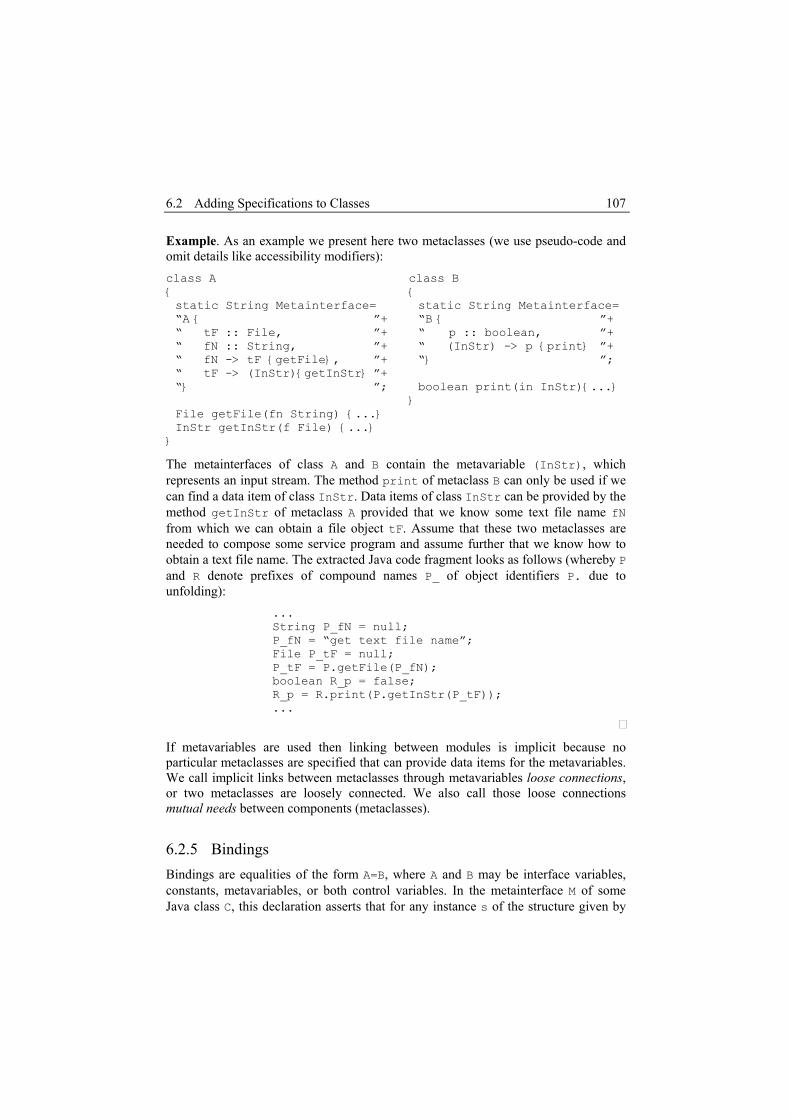
6.2 Adding Specifications to Classes 107
Example. As an example we present here two metaclasses (we use pseudo-code and omit details like accessibility modifiers): class A { static String Metainterface= “A { ”+ “ tF :: File, ”+ “ fN :: String, ”+ “ fN -> tF {getFile}, ”+ “ tF -> (InStr){getInStr} ”+ “} ”; File getFile(fn String) {...} InStr getInStr(f File) {...} }
class B { static String Metainterface= “B { ”+ “ p :: boolean, ”+ “ (InStr) -> p {print} ”+ “} ”; boolean print(in InStr){...} }
The metainterfaces of class A and B contain the metavariable (InStr), which represents an input stream. The method print of metaclass B can only be used if we can find a data item of class InStr. Data items of class InStr can be provided by the method getInStr of metaclass A provided that we know some text file name fN from which we can obtain a file object tF. Assume that these two metaclasses are needed to compose some service program and assume further that we know how to obtain a text file name. The extracted Java code fragment looks as follows (whereby P and R denote prefixes of compound names P_ of object identifiers P. due to unfolding):
... String P_fN = null; P_fN = “get text file name”; File P_tF = null; P_tF = P.getFile(P_fN); boolean R_p = false; R_p = R.print(P.getInStr(P_tF)); ...
If metavariables are used then linking between modules is implicit because no particular metaclasses are specified that can provide data items for the metavariables. We call implicit links between metaclasses through metavariables loose connections, or two metaclasses are loosely connected. We also call those loose connections mutual needs between components (metaclasses).
6.2.5 Bindings Bindings are equalities of the form A=B, where A and B may be interface variables, constants, metavariables, or both control variables. In the metainterface M of some Java class C, this declaration asserts that for any instance s of the structure given by

Chapter 6 Application to Java 108
the metainterface M, realizability of A on s is the same as realizability of B on s. Operationally, it states that, for any instance s of M, A and B of s are identical objects.
Example. As an example we present here two metaclasses (we use pseudo-code): class A { static String Metainterface= “A { ”+ “ c :: boolean, ”+ “ b :: B, ”+ “ c = b.p ”+ “ -> b {getB} ”+ “} ”; B getB() {...} }
class B { static String Metainterface= “B { ”+ “ p :: boolean, ”+ “} ”; ... }
The metainterface of class A declares two interface variables, where the data type of the interface variable b is the metaclass B whose metainterface declares the interface variable p. If the data type of an interface variable or constant is an class then we use class introspection in order to find out whether that class has a metainterface. The binding c=b.p forces c and p of b to be the same objects. Note that in this binding b refers to the structure obtained from the metainterface of class B, and not to an object identifier of an instance of class B. This is in contrast to the specification ->b of method getB where b refers to an object identifier of objects of class B. That is the reason why we write in extracted programs R_b_p instead of R.b.p, because p is not a proper attribute of class B (where R is some prefix due to unfolding).
6.2.6 Subtasks Subtasks specify functional parameters of modules. Their implementations are sub-programs with their own input and output parameters. A subtask’s realization must be synthesized when the module whose input parameter the subtask specifies is needed in the program to be composed. Since Java is an object-oriented language it suggests implementing subtasks using polymorphism, i.e., some synthesized class that extends the interface Subtask realizes a subtask. The point is that a subtask has to be associated with some class since Java is an object-oriented language, but it is not clear to which class it belongs. A subtask is passed to a method or constructor as object of Subtask rather than an object of class Method. Using Method would force a user to use reflection tools in order to execute a subtask, which is not very elegant, complicates source code, and requires sophisticated source code generation for dependent subtasks.

6.2 Adding Specifications to Classes 109
The subtask interface we use is as follows: public interface Subtask { public void subtask(Object[] in, Object[] out) throws AbortException; }
Input parameters of a subtask are passed to the subtask as array of objects (parameters are positionally mapped to array indices as they occur in the subtask specification), the output parameter is a one-element object array. The disadvantage of this approach is that we have to convert integral types to objects, which slows down synthesized programs if many subtasks with integral types are used. The method subtask of this interface may throw an abort exception, which we will explain later in connection with falsity.
We distinguish between dependent and independent subtasks (see 3.2.8 and 4.1.7). The difference between dependent and independent subtasks results in different program code. The Java programming language offers good support to implement this difference. We use inner classes for dependent subtasks and ordinary classes for independent subtasks. Inner classes are simply class definitions nested within another class or even methods. Methods and constructors of an inner class may access attributes of its encapsulating class. This corresponds to the double implication elimination inference rule for dependent subtasks (see 3.2.5). The realization of an independent subtask is encapsulated in an ordinary class whose methods and constructors cannot access attributes of the class that uses this class in some way in its definition. This corresponds to the double implication elimination rule for independent subtasks (see 3.2.8).
Example. As an example we present here a metaclass DI (double integral), Integral, and Fac (which is a metaclass that calculates some factor), where the method integral of class Integral receives a dependent subtask as an input, and the method getD of class Fac receives an independent subtask. Method integral is used twice in the metainterface DI. This example is one implementation of the double integral problem in Java, which we have already used in section 3.2.7. The additional metaclass Fac with method getD serves mainly to illustrate the difference between dependent and independent subtask implementation in Java. We explain the specifications of methods and describe the source code generation. The metainterfaces are not complete, they show only necessary specifications; the pseudo-code is shown in Figure 11.

Chapter 6 Application to Java 110
class Integral { static String Metainterface= “Integral { ”+ “ arg :: float, val : float, ”+ “ integ :: float, ”+ “ [arg -> val] -> integ {integral} ”+ ... “} ”; float integral(Subtask subtask) {...} ... }
class Fac { static String Metainterface= “Fac { ”+ “ o :: int, ”+ “ p :: int, ”+ ... “} ”; ... }
class DI { static String Metainterface= “DI { ”+ “ arg1 :: float, arg2 :: float, ”+ “ val :: float, integ :: float, ”+ “ i1 :: Integral, i2 :: Integral, ”+ “ i1.arg = arg1, i2.arg = arg2, ”+ “ i1.val = val, i2.val = i1.integ, ”+ “ integ = i2.integ, d :: int, ”+ “ d, arg1, arg2 -> val {func}, ”+ “ [Fac |- o -> p] -> d {getD} ”+ ... “} ”; float func(int i, float a1, float a2) {...} int getD(Subtask subtask) {...} ... }
We assume here that both subtasks are solvable, i.e. we can derive a realization of them by our synthesis system. The program we would like to derive is specified by the goal:
DI |- integ
We omit here to show unfolded metainterfaces and concentrate on the generated source code with a focus on subtasks. The generated source code for our goal is shown in Figure 11. Unnecessary assignments have not been removed from the program code. The class Subtask_1 is the encapsulating class of the main program, which is itself a subtask. The classes Subtask_2 and Subtask_3 are inner classes. They are defined within the class Subtask_1. The method subtask of class Subtask_3 (i.e., realization of this subtask) uses the attribute DI_i2_arg of the outer class Subtask_2 to calculate a value for DI_val. This illustrates why they are called dependent subtasks and how they can help each other. In contrast, the class Subtask_4 implements an independent subtask because Subtask_4 is not defined within any other class. As one can see from its implementation, Subtask_4 is a fresh

6.2 Adding Specifications to Classes 111
environment that uses initially only class Fac to calculate some factor. Subtask_4 cannot reuse any attributes of the other subtask classes simply because they are not known within Subtask_4. That is why Subtask_4 is called an independent subtask, i.e., it does not depend on parameters of other subtasks. Note that this subtask implementation (which is not shown here) may involve other dependent as well as independent subtasks.

Chapter 6 Application to Java 112
class Subtask_1 implements Subtask { public void subtask(Object[] in, Object[] out) throws AbortException { class Subtask_2 implements Subtask { float DI_i2_arg = 0; public void subtask(Object[] in, Object[] out) throws AbortEception { DI_i2_arg = ((Float)in[0]).floatValue(); class Subtask_3 implements Subtask { float DI_i1_arg = 0; int DI_d = 0; public void subtask(Object[] in, Object[] out) throws AbortException { DI_i1_arg = ((Float)in[0]).floatValue(); float DI_arg1 = DI_i1_arg; float DI_arg2 = DI_i2_arg; DI DI = new DI(); Subtask_4 _Subtask_4 = new Subtask_4(); DI_d = DI.getD(_Subtask_4); float DI_val = DI.func(DI_d, DI_arg1, DI_arg2); float DI_i1_val = DI_val; out[0] = new Float(DI_i1_val); } } Subtask_3 _Subtask_3 = new Subtask_3(); Integral DI_i1 = new Integral(); float DI_i1_integ = DI_i1.integral(_Subtask_3); float DI_i2_val = DI_i1_integ; out[0] = new Float(DI_i2_val); } } Subtask_2 _Subtask_2 = new Subtask_2(); Integral DI_i2 = new Integral(); float DI_i2_integ = DI_i2.integral(_Subtask_2); float DI_integ = DI_i2_integ; out[0] = new Float(DI_integ); } } class Subtask_4 implements Subtask { int Fac_o = 0; int Fac_p = 0; public void subtask(Object[] in, Object[] out) throws AbortException { Fac_o = ((Integer)in[0]).intValue(); Fac Fac = new Fac(); /* Implemenation of this independent subtask goes here, i.e. the calculation of Fac_p */ Fac_p = ...; out[0] = new Integer(Fac_p); } }
Figure 11 Java program code to illustrate double integration

6.2 Adding Specifications to Classes 113
6.2.7 Axioms We distinguish between implemented and unimplemented axioms. In Java we use constructors, instance methods, and class methods (sometime also referred to as static methods) to give realizations to implemented axioms. Unimplemented axioms can become methods only. They are similar to subtasks in the sense that they state goals to be derived, but they are implemented as regular instance methods.
Specifying instance methods is straightforward. In contrast, specified constructors and class methods need special treatment when we unfold their specifications. Simply, when we specify interface variables whose specifiers are classes, we need to be careful with their realizability. To distinguish between constructors, instance methods, and class methods while unfolding we use class introspection provided by the Java reflection tools.
Instance methods of Java classes require an instance of their corresponding class on which they have to be invoked. This does not require extra specification. Our unfolding procedure ensures that an object identifier exists for every specified instance method on which the method can be applied (see 4.3.4). To be complete we give here an example even though we have presented already some specifications of instance methods.
class A { static String Metainterface= “A { ”+ “ tF :: File, ”+ “ fN :: String, ”+ “ fN -> tF {getFile}, ”+ “} ”; File getFile(fn String) {...} }
Declaratively, the specification of the instance method getFile asserts that the structural specifcation fN->tF is realizable on instances of class A. Operationally, it states that, for any instance o of class A, fN acts as input parameter of method getFile and tF is the output parameter.
In contrast to instance methods, class methods do not require an instance of their corresponding class on which they have to be invoked; they are invoked on the class itself rather than an instance of the class. Therefore, we need to modify slightly our mapping from specifications to the logical language. The modification is the following:
{ } ( )( )
( ) ( ):
, :
pp
o pS
m a b o if m is constructor or or class methoda b m o
r m o a b o otherwise
− >− > = ∧ − >
specLL
L

Chapter 6 Application to Java 114
As an example for class methods we present here a modified version of our bank example from section 5.3. Instead of having an extra metaclass Naming we simply change the method lookup of class Naming to be a class method, which is then directly deployed in the metainterface of the metaclass Bank.
class Bank { static String Metainterface= “Bank { ”+ “ no :: long, ”+ “ url :: String, ”+ “ url -> (Bank) | (Exception) {Naming.lookup}, ”+ “ no -> (Account) | (Exception) {getAccount} ”+ “} ”; Account getAccount(long number) throws Exception {...} }
Class methods are specified by a preceding class name (Naming) in the realization (lookup) of the specification if they are used outside their defining class. The specification of the class method Naming.lookup asserts that the structural specification url->(Bank)|(Exception) is realizable on the class Naming. Operationally, it states that url acts as input parameter of method lookup and the metavariable (Bank) is the output parameter, or this method throws an exception, which we will discuss later.
Constructors require special treatment in the sense that their “return value” is always a reference to an instance of the corresponding class. Therefore, the specification of a constructor is an implication whose right-hand side must be either a metavariable whose name is the same as the class name or it must be a declared interface variable whose specifier is the respective class name. Logically, a constructor simply realizes an exitence axiom. Consider the following two metaclasses. class A { static String Metainterface= “A { ”+ “ b :: B, x :: int, ”+ “ b = (B), ”+ “ x -> b {B} ”+ “} ”; ... }
class B { static String Metainterface= “B { ”+ “ -> (B) {B} ”+ “} ”; public B() {...} public B(int i) {...} ... }
The metainterface of the metaclass A declares an interface variable b whose specifier refers to the metaclass B. The metaclass B defines two constructors where one of them is specified in the metainterface of metaclass B. There are now two ways of obtaining a proper value for the interface variable b, which is a reference to an instance of

6.2 Adding Specifications to Classes 115
metaclass B. First, by using the binding b=(B) together with the constructor specification ->(B){B}, and second, by using the specification x->b{B} which involves the unspecified constructor B(int i) of metaclass B. The first way implies that any instance of class B can serve as a proper value for b regardless how the metavariable (B) is derived. The second way explicitly specifies that the constructor B(int i) must be used. In this case the user must know that the metainterface B specifies the constructor B(int i).
Using the keyword spec in the realization part of a specification specifies unimplemented axioms. Consider the following example:
class ExchangeRate { static String Metainterface= “ExchangeRate { “ currency :: String, ”+ “ exchangeRate :: float, ”+ “ exch :: Exchange, ”+ “ exch = (Exchange), ”+ “ exch.currency = currency, ”+ “ exch.exchangeRate = exchangeRate, ”+ “ currency -> exchangeRate {spec} ”+ “} ”; }
If the unimplemented axiom for calculating the exchangeRate for a given currency is needed to synthesize some Java program, then a new goal (which is given by the specification of this axiom) is issued. The realization of this goal gives the implementation of the unimplemented axiom. This implementation is put into a new instance method with some arbitrary name. This new method is then used in a regular way.
In terms of services unimplemented methods are suitable for specifying new service configurations from existing components when additional methods and constructors are not needed.
6.2.8 Using Control Variables A control variable is simply a name enclosed by square brackets. Control variables do not refer to any constant or interface variable. Moreover, they do not become attributes of classes of composed Java programs. We use control variables to add extra logical conditions to axioms in order to force the order of application of modules. For Java, this is particularly useful for specifying void methods, i.e., methods with void input and output. Without control variables we could not use those methods, because then the specification of a module would be limited to its parameters, which void methods do not have.

Chapter 6 Application to Java 116
Example. We use here a modified version of the example from section 6.2.4. Only the metainterface of class B has been changed slightly. The metaclasses are the following (we use pseudo-code and omit details like accessibility modifiers): class A { static String Metainterface= “A { ”+ “ tF :: File, ”+ “ fN :: String, ”+ “ fN -> tF {getFile}, ”+ “ tF -> (InStr){getInStr} ”+ “} ”; File getFile(fn String) {...} InStr getInStr(f File) {...} }
class B { static String Metainterface= “B { ”+ “ (InStr) -> [p]{print} ”+ “} ”; void print(in InStr) {...} }
In the metainterface of class B we removed the interface variable p and modified the specification of method print by replacing the interface variable p with the control variable [p]. The method print thus becomes a void method, which is the usual realization in Java for such methods.
Example. Assume we want to force the order of invocation of two modules that could be executed in any order according to their parameters, e.g., because they do not have common parameters. Consider the metaclass C. class C { public static String Metainterface = “C { ” + “ inf :: java.net.InetAddress, addr :: java.net.InetAddress, ” + “ port :: int, ” + “ connected :: boolean, ” + “ inf -> [initialized] {init}, ” + “ [initialized], addr, port -> connected {connect} ” + “} ”; void init(java.net.InetAddress inf) {...} boolead connect(java.net.InetAddress addr ,int port) {...} }
If the control variable [initialized] would not be a precondition of the method connect, we may derive a program which first connects to the destination host and afterwards initializes the outgoing interface on which the connection should be made.
This pattern of specification is often needed for initializing some object when the specific way of initialization matters or when we want to specify what is needed to

6.2 Adding Specifications to Classes 117
execute before and what is possible to execute after execution of some module. For instance, there are some classes in Java that can be instantiated in several ways, but the possible invocations of their methods and especially their order of invocation depends on how the instance of the class has originally been created.
6.2.9 Exceptions Constructors and methods may throw exceptions. To specify this we use disjunction on the right hand-side of the main implication of a specification of a constructor or method, where the first alternative must specify the actual output that can be a control variable, interface variable, or metavariable, and the other alternatives must all be metavariables or declared interface variables that specify classes that extend the class java.lang.Exception. Any alternative may be followed by a list of control variables.
Example. We extend the metaclass Bank from above as follows: public interface Bank extends java.rmi.Remote { static String Metainterface= “Bank { ”+ “ no :: long, ”+ “ url :: String, ”+ “ nbe :: java.rmi.NotBoundException, ”+ “ mue :: java.net.MalformedURLException, ”+ “ url -> (Bank) | nbe | mue | (java.rmi.RemoteException) {java.rmi.Naming.lookup}, ”+ “ no -> (Account) | (Exception) {getAccount}, ”+ “ nbe -> falsity {handleNotBound}, ”+ “ mue -> falsity {handleMFURL} ”+ “} ”; Account getAccount(long number) throws Exception; void handleNotBound(NotBoundException e); void handleMFURL(MalformedURLException e); }
The metaclass Bank has been changed to be a java RMI remote interface. The specification of the deployed class method java.rmi.Naming.lookup has been extended with a more detailed specification regarding possible exceptions for NotBoundException and MalformedURLException we use two special exception handlers handleNotBound and handeMFURL, respectively. After handling one of these two exceptions this metainterface specifies that we must abort the transaction, which is specified by falsity. In case of RemoteException another exception handler must be used but it is not specified explicitly which one is to be used.
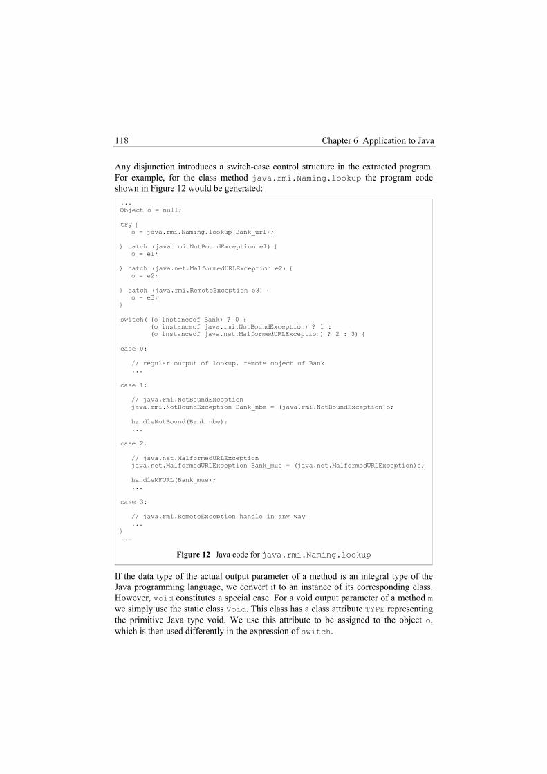
Chapter 6 Application to Java 118
Any disjunction introduces a switch-case control structure in the extracted program. For example, for the class method java.rmi.Naming.lookup the program code shown in Figure 12 would be generated: ... Object o = null; try { o = java.rmi.Naming.lookup(Bank_url); } catch (java.rmi.NotBoundException e1) { o = e1; } catch (java.net.MalformedURLException e2) { o = e2; } catch (java.rmi.RemoteException e3) { o = e3; } switch( (o instanceof Bank) ? 0 : (o instanceof java.rmi.NotBoundException) ? 1 : (o instanceof java.net.MalformedURLException) ? 2 : 3) { case 0: // regular output of lookup, remote object of Bank ... case 1: // java.rmi.NotBoundException java.rmi.NotBoundException Bank_nbe = (java.rmi.NotBoundException)o; handleNotBound(Bank_nbe); ... case 2: // java.net.MalformedURLException java.net.MalformedURLException Bank_mue = (java.net.MalformedURLException)o; handleMFURL(Bank_mue); ... case 3: // java.rmi.RemoteException handle in any way ... } ...
Figure 12 Java code for java.rmi.Naming.lookup
If the data type of the actual output parameter of a method is an integral type of the Java programming language, we convert it to an instance of its corresponding class. However, void constitutes a special case. For a void output parameter of a method m we simply use the static class Void. This class has a class attribute TYPE representing the primitive Java type void. We use this attribute to be assigned to the object o, which is then used differently in the expression of switch.

6.2 Adding Specifications to Classes 119
... try { m(...); o = Void.TYPE; } catch (...) { ... } switch (((Class)o == Void.TYPE) ? 0 : ...) { case 0: ... } ...
The Void class is an uninstantiable placeholder class to hold a reference to the class object representing the primitive Java type void; therefore one has to use the detour via the Class object. All other primitive Java types are convertible into their corresponding class. For instance, if the output parameter of a method m is an integer, then we generate this code:
... try { o = new Interger(m(...)); } catch (...) { ... } switch ((o instanceof Integer) ? 0 : ...) { case 0: ... } ...
Special care must be taken if we specify exceptions. The problem is that any exception class must extend the class Exception to define a throwable object. This could be a source of “wrong” code generation if class introspection is not used for determining the inheritance hierarchy of exception classes. For instance, let us assume a method m throws three different exceptions, but we are only interested in handling one of them in a special way. All other exceptions can be handled in any way. Consider the following metaclass C:

Chapter 6 Application to Java 120
class C { static String Metainterface= “C { ”+ “ ire : InterruptedException, ”+ “ -> [succeeded] | (Exception) | ire {m}, ”+ “ ire -> (Exception) {handleIRE} ”+ “} ”; void m() throws InterruptedException, ClassNotFoundException, SecurityException {...} Exception handleIRE (InterruptedException e) }
The following “wrong” program code might be generated if we are not taking into account inheritance hierarchy of exception classes:
... Object o = null; try { m(); o = Void.TYPE; } catch (InterruptedException ire) { o = ire; } catch (ClassNotFoundException e1) { o = e1; } catch (SecurityException e2) { o = e2; } switch ( ((Class)o == Void.TYPE) ? 0 : (o instanceof Exception) ? 1 : 2) { case 0: ... case 1: ... case 2: ... } ...
The flaw is that whatever exception method m throws the second branch of the switch (case 1) would always be taken because every object of any exception class is also an instance of class Exception.
Source code generation should use class introspection to determine the inheritance hierarchy of exception classes in order to generate the appropriate branch structure for switch statements. The strategy for source code generation is to put first the tests for exception classes that are lowest in the inheritance hierarchy.

6.2 Adding Specifications to Classes 121
6.2.10 Falsity If we use the constant falsity in the specification of any method and this specification is involved in program composition, then our synthesis system will generate an algorithm which will abort the current branch of computation after this method has been executed. This corresponds to the falsity elimination rule of our inference system (see section 3.3.4). In Java we abort computation by throwing an abort exception. One has to be carefully with use of falsity in specifications. We recommend using falsity only in specifications of exception handlers; otherwise one might derive meaningless programs.
There are two problems. One is that we have to signal the abort to the outer program code that entered the branch of computation where the abort occurred. The other problem is related to unimplemented axioms. If an abort occurs in the realization of an unimplemented axiom then it is not yet clear how to deal with this abort.
Let us investigate the first case. A branch is a subtask. The environment that entered a branch is a pre-programmed method or constructor. Since the method subtask of the subtask interface may throw an AbortException the calling environment must catch this exception. The class AbortException belongs to the synthesis system. The calling environment then has the possibility to deal with this abort exception in the regular way of handling exceptions in Java, i.e., a method or constructor that entered the subtask method must catch a possible abort exception before continuing computation or the abort exception is propagated upwards the chain of method calls as usual.
Example. For instance the definition of method integral of the metaclass Integral from above must contain the following code:
class Integral { static String Metainterface= “Integral { ”+ “ arg :: float, val :: float, integ :: float, ”+ “ [arg -> val] -> integ {integral} ”+ “} ”; float integral(Subtask subtask) { ... try { subtask.subtask(..., ...); } catch (AbortException ae) { ... } ... } ... }

Chapter 6 Application to Java 122
The cases one and two of our java.rmi.Naming.lookup example from above must be extended with throw clauses to throw an abort exception at the end of these two branches. case 1: // java.rmi.NotBoundException java.rmi.NotBoundException Bank_nbe = (java.rmi.NotBoundException)o; handleNotBound(Bank_nbe); throw new AbortException(Bank_nbe); case 2: // java.net.MalformedURLException java.net.MalformedURLException Bank_mue = (java.net.MalformedURLException)o; handleMFURL(Bank_mue); throw new AbortException(Bank_mue);
Now we will investigate the second problem related to unimplemented axioms, which is exposed by the fact that we are not aware of occurrences of exceptions at specification time. If a method or constructor throws an exception then it must be specified using a disjunction. Subtasks may throw abort exceptions if falsity is specified as result of some method that is executed by the subtask. Every realization of unimplemented axioms is executed within a subtask, which is ensured by the fact that the main program of a synthesized Java program is a subtask. An implementation of an unimplemented axiom derived by our synthesis system is a method that we supply with a throw clause in its signature. Then, whenever an abort exception inside the synthesized method occurs, this abort exception will be propagated as usual in Java. The program code (environment) that entered the corresponding subtask then catches this abort exception.
Example. Assume we have given the following specification of an unimplemented axiom: [init]->level{spec}. Let level be a declared interface variable whose specifier is int. Whenever this specification is involved in the synthesis of a program then it is defined in some subtask class as follows:
... class Subtask_n implements Subtask { void spec_m (int i) throws AbortException{ ... throw new AbortException(...); } public void subtask(Object[] in, Object[] out) throws AbortException { spec_m(...); } } ...

6.2 Adding Specifications to Classes 123
If an abort exception occurs during the given call of spec_m then this abort exception will be forwarded to the environment that called the subtask Subtask_n because the call of spec_m in method subtask of class Subtask_n does not occur within a try-catch statement.
6.2.11 Inheritance Inheritance for metainterfaces is the same as inheritance for Java classes. A Java class or interface that extends or implements a metaclass is a metaclass (Java interfaces that are supplied with a metainterface are considered to be metaclasses as well). A metaclass that extends or implements some metaclass inherits all specifications of all super-metainterfaces in the class hierarchy.
Inheritance of metainterfaces allows us to extend and modify specifications of classes. For instance, one can think of a metaclass that does not implement any new method but overrides some specifications of its superclass. When a metaclass inherits the metainterface of its superclass, naming conflicts of control variables, constants, and interface variables may occur. In such a case the respective interface variable, control variable, or constant of the metainterface of the superclass is shadowed which requires renaming of constants and variables of the extending class. It is obviously not possible to consider constants and (control and interface) variables of the metainterface of the extending class and the metainterface of the superclass to be the same for two reasons. First, the respective specifier of a constant or interface variable may be different, and second, the conceptual usage may be different in the superclass. Renaming is needed since we use unfolding that flattens all configuration hierarchies of metainterfaces. At the same time, renaming is safe since it does not change conceptual usage of constants, interface variables, and control variables, and the specification language does not allow specifications of metainterfaces to refer to constants and variables of metainterfaces of superclasses.
Due to the fact that a Java class may extend a class and implement interfaces at the same time and we support inheritance of metainterfaces, we have to deal with multiple inheritances. If any collision between specified methods occur while unfolding, then we change the realization of the respective method specification in the following way: The realization of an instance method m after unfolding is a tuple (r,m) where r specifies the object on which method m must be invoked. If a method collision occurs we cast the object r to the respective class. Let r be of class C, m be defined in class A such that it collides with some other method m and C extend A, then the realization of the respective specification is changed to ((A)r,m), which results in expressions of the form ((A)o).m(…) in the extracted programs.
Class methods are no problem because they are invoked on the class rather than an instance of the class; hence, invoking them on their defining class can easily prevent collisions. For example, let m be defined in class A such that it collides with some

Chapter 6 Application to Java 124
other method m and C extends A, then the realization C.m of the respective specification is changed to A.m.
6.2.12 Overriding Overriding in metainterfaces is allowed but it needs special treatment. In general nine cases are possible, where the specification language does not allow three of them. These three cases are given when the metainterface of a metaclass specifies methods of some other metaclass that extends this metaclass, which is not possible. The following are the other six possible cases:
1) The metainterface of a metaclass specifies a method of the superclass, which is not overridden and not specified in the metainterface of the superclass.
2) The method is overridden but not the specification.
3) Only the method is overridden.
4) The metainterface of a metaclass specifies a method, which is not overridden, but specified in the metainterface of the superclass as well, i.e. only the specification of this method is overridden in the metainterface.
5) The metainterface of a metaclass specifies a method that is overridden and specified in the metainterface of the superclass as well.
6) The method is overridden and specified in the metainterface of the superclass.
We can summarize these cases in the following table:
Table 11 Inheritance in metainterfaces Class Superclass Metainterface Method Metainterface Method
1 × × 2 × × × 3 × × 4 × × × 5 × × × × 6 × × ×
The column heading Class denotes the metaclass that extends or implements Superclass (superclass or implemented interface). A cross in a cell of any column Metainterface means a specification of the method exists in the metainterface of the corresponding class, and a cross in a cell of any column Method means the method is implemented in the respective class, which is either the superclass or the class that extends this superclass.
Case one does not exhibit any difficulties because a metainterface of class may specify a method of the superclass. The second case specifies the overridden method,

6.3 Program Extraction 125
no ambiguities occur because Java guarantees that the overridden method is used in computation whenever we use this class in synthesized programs. No specification overriding is involved in the third case. In case four only the specification is overridden. In this case the specification of the superclass is simply discarded. Case five is a combination of case 2 and case four. Both, specification and method are overridden, where as for case four the specification of the superclass is discarded and Java guarantees that the overridden method is used in computation whenever we use this class in synthesized programs. The critical case is six, which we have therefore grayed. The problem here is that after unfolding we obtain a specification of a method of the extending class that does probably not match the intended conceptual usage, which is denoted by the specification, of the method of the superclass. Fortunately, this situation can be detected automatically by introspection of classes while unfolding. In this case we change the realizer of the specifcation as we have explained in the previous subsection.
Overriding in metainterfaces requires strict top down unfolding of superclasses and implemented interfaces. In other words, the superclasses and interfaces (which are metaclasses) occurring on top of the inheritance hierarchy must be unfolded first and then their extending metaclasses gradually added.
6.2.13 Overloading Overloading of specifications of methods and constructors is possible without any restrictions.
6.3 Program Extraction
Every synthesized Java program (class) implements the subtask interface. This facilitates deployment of synthesized programs and enables us at the same time to invoke the synthesis process within other Java programs, which is similar to the method compute of the NUT language (Uustalu 1995b). Essentially, the method compute can be seen as a generic unimplemented method that invokes synthesis for a given goal (i.e., the specification of the program to be synthesized) and then executes this program if it exists.
Java program extraction is straightforward. We do without examples when describing program extraction because we have already given examples for every possible case. From the synthesizer we obtain an algorithm (which is extracted from the proof of existence of the desired program). According to the structural synthesis rules of our logic (see 3.3.4), an instruction of such an algorithm may be either a module (constructor or method) application or a case-statement. A module application may be passed a sub-program (subtask). In this case we generate a new class that implements the subtask interface and implements the needed sub-program. This subtask class is an inner class if a dependent subtask is needed and it is a top-level class if an

Chapter 6 Application to Java 126
independent subtask is required. Inner classes implementing dependent subtasks are inserted into the Java program code directly before method or constructor application.
We declare an attribute for each interface variable in the current subtask class definition if this interface variable is an input parameter of the current subtask. Inputs of subtasks (realizations of hypothesis) are assigned to their respective attribute. These assignments are the first statements of the subtask implementation, i.e. in the method subtask. Other interface variables that specify input/outputs of methods and constructors become local variables. Attributes and local variables realizing an interface variable are single assignment variables. (Sometimes also called logical variables, or simply dataflow variables.) Method and constructor invocations are inserted into the program according to the algorithm.
Due to bindings (equalities) occurring in specifications unnecessary assignments may be introduced in the program code if we follow strictly program extraction as described above. Therefore, if computability of an interface variables is derived due to equality with another interface variable then we use the latter one instead, which is justified by the fact that the other interface variable must have been used before by program extraction. This simply guarantees that interface variables bound by equality identify the same object.
6.4 Synthesis of Java Programs
Java classes and interfaces are the unifying implementation concept for logic and components. Everything is represented in the form of a metaclass (where Java classes and Java interfaces that are supplied with a metainterface are considered to be a metaclass): a component is a metaclass, the implementation of a synthesized Java program is a metaclass, and a logical specification of a component is represented by a static attribute Metainterface in its class. We can think about this logical part as a separate declarative view of a component. This part is not used in computations but only for composing implementations of Java programs. On the other hand, the logic of synthesis is completely determined by the logical specification given in the Metainterface and the synthesis process does not use the actual Java class4. Synthesis is processed on the logical part of a class, i.e., on the metainterface of a class, and its methods and constructors are used in the program implementation. To specify a new Java program, one has to compose manually a new metaclass (C2) from available metaclasses (C1, C3) and classes.
4 Before synthesis takes place we use the actual class but only for unfolding of specifications
where we use class introspection. Unfolding is not synthesis.

6.4 Synthesis of Java Programs 127
C3
C2
Linked explicitly by spec
Linked by synnthesis
C1
Figure 13 Specifying a new Java program
When specifying a new Java program links (solid line) between components can be given explicitly, but they can also be detected automatically using first-order features of our specification logic, i.e., using metavariables (broken line) of our specification language, Figure 13. The Java program becomes a new class, which implements the Java interface Subtask. The (synthesized) method subtask of this new class implements the desired program.
Synthesis of Java programs works essentially as described in Chapter 5. All metainterfaces are unfolded before synthesis. Additionally, unfolding now also includes inheritance, i.e., unfolding now works in two directions, first the upward direction, unfolding of superclasses and implemented interfaces using the Java-specific class introspection tools, and second, unfolding of the aggregation hierarchy built by the metainterfaces. Figure 14 depicts the steps of the actual synthesis process.
:: : : :: ( ) : : ( ) :
: , : ( ( ), ( )) :. ( ( ), ( )) :
f A B g U Va A a A u U u Ua A f a B u U g u V
a A u U h f a g u Xau h f a g u A U Xλ
⊃ ⊃
∧ ⊃
0 00 000 0
00
Proof (2):
::h B V X∧ ⊃
Java program (4): class Subtask_1 implements Subtask { ... }
Algorithm extraction (3):1) apply f on a A 2) apply g on a U 3) apply h on the result
of f and g
Theory (1): : f:A⊃B g:U⊃V h:B∧V⊃X
Figure 14 Steps of synthesis process
From a formal theory (1) (which we derive from unfolding of metainterfaces of classes and translation of specification expressions into our logical language) and a given synthesis problem (in form of a program specification) we try to prove (2) the existence of the specified program. If such a program exists we extract from the proof

Chapter 6 Application to Java 128
an algorithm (3), which is represented in the form of an abstract syntax tree (Batory, Lofaso, and Smaragdakis 1998). The algorithm can then be translated (4) into Java program code.
6.5 Performance of Synthesis
This subsection presents one experiment with a prototype implementation of the Java program synthesizer, which works on the declarative specification language described in Chapter 4. The purpose of this experiment was to validate the proposed approach to runtime service composition by presenting performance measurements under a test set that correspond to practical service composition problems. This experiment analysed three different performance aspects. First, we investigated the runtime performance of the synthesis system itself, second, we measured the time needed for program extraction, and third we compared the execution time of a synthesized program and its “hand-coded” counterpart.
6.5.1 Environment To carry out our experiments we used a Sun Microsystems Enterprise Server 4000 with 1.5 GB main memory, 166MHz CPU speed, and operating system SunOS 5.6. We used the Java developer kit JDK 1.2.1. The decision to use the Sun enterprise server was motivated by its large main memory, which we need to avoid the distortion of measured time due to memory swapping of the operating system. The Java virtual machine occupied at most 16MB memory. During experimentation we did not have an exclusive use to the Sun enterprise server. A number of other applications were running on it at the same time.
6.5.2 Test Set The specification for every synthesis problem in this experiment is represented as a single Java class. This is not a substantial restriction, since the specifications are unfolded before synthesis; hence, in terms of synthesis time there should be no difference between using a single class and using multiple classes. All Java classes of our synthesis test set were automatically generated. In our experiment we wanted to compare the execution time of a synthesized Java program with the execution time of its hand-coded counterpart. For this purpose we generated also Java programs in hand-coded style.
6.5.2.1 Synthesis Problems The metaclasses we have used for synthesis contain two kinds of methods, methods with one input parameter of data type int, and methods with two input parameters,
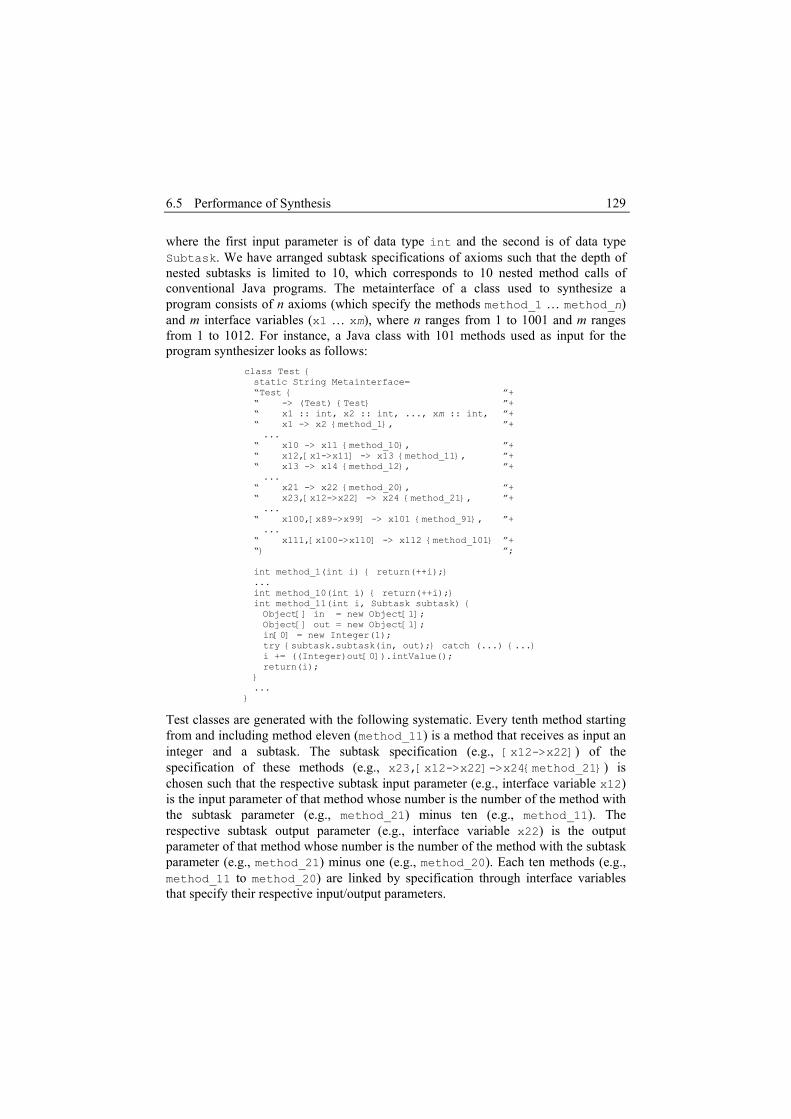
6.5 Performance of Synthesis 129
where the first input parameter is of data type int and the second is of data type Subtask. We have arranged subtask specifications of axioms such that the depth of nested subtasks is limited to 10, which corresponds to 10 nested method calls of conventional Java programs. The metainterface of a class used to synthesize a program consists of n axioms (which specify the methods method_1 … method_n) and m interface variables (x1 … xm), where n ranges from 1 to 1001 and m ranges from 1 to 1012. For instance, a Java class with 101 methods used as input for the program synthesizer looks as follows:
class Test { static String Metainterface= “Test { ”+ “ -> (Test) {Test} ”+ “ x1 :: int, x2 :: int, ..., xm :: int, ”+ “ x1 -> x2 {method_1}, ”+ ... “ x10 -> x11 {method_10}, ”+ “ x12,[x1->x11] -> x13 {method_11}, ”+ “ x13 -> x14 {method_12}, ”+ ... “ x21 -> x22 {method_20}, ”+ “ x23,[x12->x22] -> x24 {method_21}, ”+ ... “ x100,[x89->x99] -> x101 {method_91}, ”+ ... “ x111,[x100->x110] -> x112 {method_101} ”+ “} ”; int method_1(int i) { return(++i);} ... int method_10(int i) { return(++i);} int method_11(int i, Subtask subtask) { Object[] in = new Object[1]; Object[] out = new Object[1]; in[0] = new Integer(1); try {subtask.subtask(in, out);} catch (...) {...} i += ((Integer)out[0]).intValue(); return(i); } ... }
Test classes are generated with the following systematic. Every tenth method starting from and including method eleven (method_11) is a method that receives as input an integer and a subtask. The subtask specification (e.g., [x12->x22]) of the specification of these methods (e.g., x23,[x12->x22]->x24{method_21}) is chosen such that the respective subtask input parameter (e.g., interface variable x12) is the input parameter of that method whose number is the number of the method with the subtask parameter (e.g., method_21) minus ten (e.g., method_11). The respective subtask output parameter (e.g., interface variable x22) is the output parameter of that method whose number is the number of the method with the subtask parameter (e.g., method_21) minus one (e.g., method_20). Each ten methods (e.g., method_11 to method_20) are linked by specification through interface variables that specify their respective input/output parameters.

Chapter 6 Application to Java 130
The input and output parameters (which are specified by interface variables, e.g., x111 and x112) of primitive data type of the last method of each test class (e.g., method_101) are used to specify the program to be synthesized. For instance, if we use the class Test presented above as input for synthesis then we write the goal
Test |- x111 -> x112
The test set we have chosen is typical for services; because every runtime composable service must possess an intrinsic service flow from one runtime entity (component) to another, which is an assumption of this work, see section 1.2.1 and 2.4.3. Our test classes have such an intrinsic service flow. On the one hand we could not find any practical example of a service that requires complicated subtask dependencies (even though such examples exist in theory); hence, our test set contains no sophisticated subtask dependencies that may cause very complex proof search. On the other hand the really hard problems occur on the boundary between an underconstrained problem region and an overconstrained problem region of a certain problem domain (which is for us polynomial-space complete). The density of solutions of the underconstrained region is high, thus making it easy to find solutions. The overconstrained region is very unlikely to contain a solution. If there is a problem solution, then any reasonable algorithm is likely to find it. The probability of solution on the boundary between these two regions is low but non-negligible (Cheeseman, Kanefsky, and Taylor 1991). We argue that for our problem domain the boundary between the underconstrained and over constrained region contains problems that are not tractable for services. For instance, a not tractable specification for services would contain many axioms like [a->b]->c{m} that are hardly linked by interface variables. Such a specification does not possess an intrinsic service flow, and is therefore not tractable for services.

6.5 Performance of Synthesis 131
6.5.2.2 Synthesized Programs Here we show the Java program that has been synthesized from the class Test, which we have presented above. The method subtask of the class Subtask_1 implements this program.
class Subtask_1 implements Subtask { int Test_x111 = 0; public void subtask(Object[] in, Object[] out) throws AbortException { Test_x111 = ((Integer)in[0]).intValue(); class Subtask_2 implements Subtask { int Test_x100 = 0; public void subtask(Object[] in, Object[] out) throws AbortEception { Test_x100 = ((Integer)in[0]).intValue(); class Subtask_3 implements Subtask { ... class Subtask_11 implements Subtask { int Test_x1 = 0; public void subtask(Object[] in, Object[] out) throws AbortEception { Test_x1 = ((Integer)in[0]).intValue(); Test _Test = new Test(); int Test_x2 = _Test.method_1(Test_x1); int Test_x3 = _Test.method_2(Test_x2); ... int Test_x10 = ... int Test_x11 = _Test.method_10(Test_x10); out[0] = new Integer(Test_x11); } } ... } Test _Test = new Test(); Subtask_3 _Subtask_3 = new Subtask_3(); int Test_x101 = _Test.method_91(Test_x100, _Subtask_3); int Test_x102 = _Test.method_92(Test_x101); ... int Test_x109 = ... int Test_x110 = _Test.method_100(Test_x109); out[0] = new Integer(Test_x110); } } Test _Test = new Test(); Subtask_2 _Subtask_2 = new Subtask_2(); int Test_x112 = _Test.method_101(Test_x111, _Subtask_2); out[0] = new Integer(Test_x112); } }

Chapter 6 Application to Java 132
6.5.2.3 Hand-coded Programs With “hand-coded” programs we mean automatically generated Java programs that have essentially the same structure as their synthesized counterparts, but they use direct method calls instead of receiving subtask objects as inputs and then invoking the method subtask on these subtask objects. We also say that method calls are hardwired into the method definitions. A subtask of a synthesized program corresponds to a regular method in a hand-coded program. Hand-coded programs do also not convert elements of primitive data type into their corresponding objects. So, in this sense hand-coded programs are not really hand-coded, but they follow the style of coding programs by hand, and therefore, they reflect to some extend realistic programming practices.
For instance, a hand-coded Java program with 101 methods is represented as a primary Java class5 and looks as follows:
class Test { int method_1(int i) { return(++i);} ... int method_10(int i) { return(++i);} int subtask_1_10 (int i) { return(method_10(method_9(...(method_1(i))...))); } int method_11(int i) { i += subtask_1_10(1); return(i); } ... int subtask_91_100 (int i) { return(method_100(method_99(...(method_91(i))...))); }
int method_101(int i) { i += subtask_91_100(1); return(i); } public static void main(String[] args) { try { (new Test()).method_101(Integer.parseInt(args[0])); } catch (Exception e) { System.err.println(e); } } }
This primary Java class defines additionally “subtask”-methods (e.g., subtask_91_100) that correspond to and emulate subtasks of synthesized programs.
5 A primary Java class is a regular Java class that contains a main method. This main method
is executed by the Java Virtual Machine (JVM) and can be used to start up a Java program.

6.5 Performance of Synthesis 133
Subtask calls are regular method calls. Compare the structure of this primary class with the structure of the synthesized Java program of the previous subsection. Subtask-methods of this primary class are inner classes (subtask classes) in synthesized programs. The body of subtask-methods and the corresponding method subtask of Subtask classes of the synthesized program example from above are basically the same.
6.5.3 Expected Results Synthesis time Since the complexity of intuitionistic logic is polynomial-space complete (P-SPACE) (Statman 1979, Buss and Mints 1999) we should expect that the time needed for synthesis grows exponentially depending on the depth of dependent subtasks. But for this particular test set we should observe a linear growth of synthesis time depending on the size of specification.
Program extraction time Program extraction involves algorithm extraction from the proof of existence of the desired program and generating Java program code from that algorithm. From unfolding of specifications we obtain prior synthesis sufficient information (e.g., typing) that is needed for program code generation. Additional class introspection is therefore not needed for program extraction. We can expect that algorithm extraction and program code generation is faster than proof search.
Program execution time The depth of nested subtasks determines the depth of nested subtask classes in synthesized programs and determines the depth of method calls in hand-coded programs. Synthesized Java programs with low depth of nested subtasks should show a slightly increased execution time compared to their respective hand-coded counterparts. This has two reasons. First, we must convert parameters of subtasks that are of primitive data type into corresponding objects and all output and input parameters of subtasks are passed to the subtask method through an object array. Converting elements of primitive data types into their corresponding objects costs time and memory. Second, methods and constructors of hand-coded Java programs do usually not receive methods as input to be executed within their respective definition. Calls of methods are hard-wired in the definition. These additional overheads, which are due to the usage of subtasks instead of direct method calls, should cause a longer execution time of synthesized programs.
6.5.4 Measurements The following chart (Figure 15) shows the times needed for synthesis and program extraction as well as the execution times of synthesized Java programs and their respective hand-coded programs.

Chapter 6 Application to Java 134
Synthesis / Extraction / Execution
0
100
200
300
400
500
600
10 100 190 280 370 460 550 640 730 820 910 1000
Number of methods
Tim
e in
ms
Synthesis
Program extraction
Hand-coded program execution
Synthesized program execution
Synthesis + Extraction + Execution
Figure 15 Performance measurements
All experiments have been repeated three times and the average measurement value has been taken. Time needed for starting up the Java virtual machine is assumed to be a constant and neither taken into account nor shown in the chart.
Our prototype implementation generates Java program source code. The Java programs are generated from an abstract syntax tree representing the synthesized algorithm. We refer to this transformation step as “program extraction”. We did not take into account time needed for compiling generated Java programs. In a real implementation, however, we would generate byte-code directly from a synthesized algorithm such that the detour via Java program source code is not needed. Therefore, we can assume that the time measured for program extraction in our experiments represents approximately the program extraction time in a real implementation.
6.5.5 Analyses The two lowermost data series (labeled Synthesized program execution and Hand-coded program execution) show the difference in execution time between a synthesized Java program and the respective hand-coded program. For both cases, execution time grows linearly with increasing number of methods. The average difference of execution time is about 10ms. This difference can be explained by the computational overhead needed for converting values of primitive data types into instances of their corresponding classes, and for using classes for subtask implementations. This computational overhead cannot be avoided by code optimization for instance, because

6.5 Performance of Synthesis 135
we cannot assume to have access to source code of components (metaclasses and classes).
The two data series labeled Synthesis and Program extraction represent performance of the two stages of the synthesis process. The first stage is synthesis, which refers to the search for the existence proof of the requested program that is at the same time recording the algorithm. The second stage is program extraction, which refers to the translation of the algorithm into an executable program. Synthesis time and program extraction time increase linearly with growing number of axioms (which is for this particular case the same as the number of methods). For this particular test set and test environment we have measured a parallel and linear growth of synthesis time and program extraction time. This parallel growth can be explained by the kind of test set we have chosen, because every step of search for the existence proof corresponds to a step of source code generation and every test class contains as many method specifications (axioms) as needed to synthesize the desired program. However, we have also carried out other experiments with different test sets (which are not tractable for services) where synthesis time grows polynomially and program extraction grows linearly until a certain threshold (from which we do not know exactly on what is depends) is reached, and then program extraction grows even exponentially. The linear growth of synthesis can be explained by the test set as well. This test set does not cause backtracking in the proof search, because axioms with subtask specifications (which might introduce backtracking) also contain an interface variable in their respective precondition. These interface variables are extra constraints and act like guards. It is our proof search strategy to use a formula (axiom) with nested implication (subtask specification) only if all other propositions (interface variables and control variables) occurring in the premise of the main implication of this formula (axiom) are derivable (realizable, computable). This explains why these interface variables act like guards and why proof search (synthesis) is linear in the size of the specifications of this particular test set.
The uppermost data series (labeled Synthesis+Extraction+Execution) of the chart above (Figure 15) is the sum of the times needed for synthesis, program extraction, and program execution for a given problem, or in terms of services, for a service request that also specifies the required service. The sum of these three quantities represents the general response time or service latency a user experiences if our approach to program synthesis is used for runtime service composition. For this particular test set, the time needed for the complete synthesis process plus program execution time depends linearly on the number of axioms of a given specification if the number of subtasks is constant.


Chap t e r 7
Application to Runtime Service Composition
In this chapter we present the application of our program synthesis approach to runtime service composition using Java as programming language by describing two more examples, a print service and stock quote cache. We already introduced the print service example in section 3.3 and conceptually described the stock quote cache in section 2.5.
When describing these examples we do not show the algorithmic parts of the constructors and methods of the metaclasses but rather concentrate on specifications and composition. We also assume that any component in the system propagates its metainterface to the runtime service composition service in some way, which we do not describe. In distributed systems, metainterfaces are frequently added to the environment and removed from the environment, which results in changing service environments. Keeping information about available resources and service interfaces (in our case metainterfaces) in a distributed system consistent is a current but different research topic in peer-to-peer computing.
In general modules of components (methods and constructors of Java classes) should be executed at the side of the service point, i.e., at this network node where the respective service component resides. This gives platform independence, at least to a large extent. A distribution layer that provides platform and programming language independent data representation, for example CORBA, must be used to pass data
137

Chapter 7 Application to Runtime Service Composition 138
objects between distributed components. If components are not distributed objects for which we can invoke remote modules, additional instructions related to data distribution will be needed in extracted programs. In this case, the instructions of a composed service program are distributed as well, which requires dataflow synchronization. This results in highly distributed composed service programs, which we cannot extract in the conventional way. But the algorithm obtained from the synthesis process gives us a plan that we can use to coordinate execution of distributed modules. We will investigate this in Chapter 8.
7.1 A Print Service
Our print service example involves two remote components, a print server component that has access to a printer, and a client that asks for print service. Both components implement a remote interface. These remote interfaces are metaclasses. The actual implementation of these two interfaces is uninteresting for us. The specifications used in this example were also used in section 3.3. However, we have slightly modified them here to reflect their Java-implementations better. Essentially, we extended the specifications with disjunctions due to remote exceptions.
The printer server’s remote interface is supplied with a metainterface as follows:
import java.rmi.Remote; import java.rmi.RemoteException; public interface PrintServer extends Remote { static String Metainterface= “PrintServer { ”+ “ o :: Printable, ”+ “ -> (PrinterType) | (RemoteException) { getPT }, ”+ “ (RemoteFile),(Converter) -> o | (RemoteException) { convert }, ”+ “ o -> (PrintReport) | (RemoteException) { print } ”+ “} ”; public PrinterType getPT() throws RemoteException; public Printable convert (RemoteFile rf, Converter c) throws RemoteException; public PrintReport print (Printable o) throws RemoteException; }
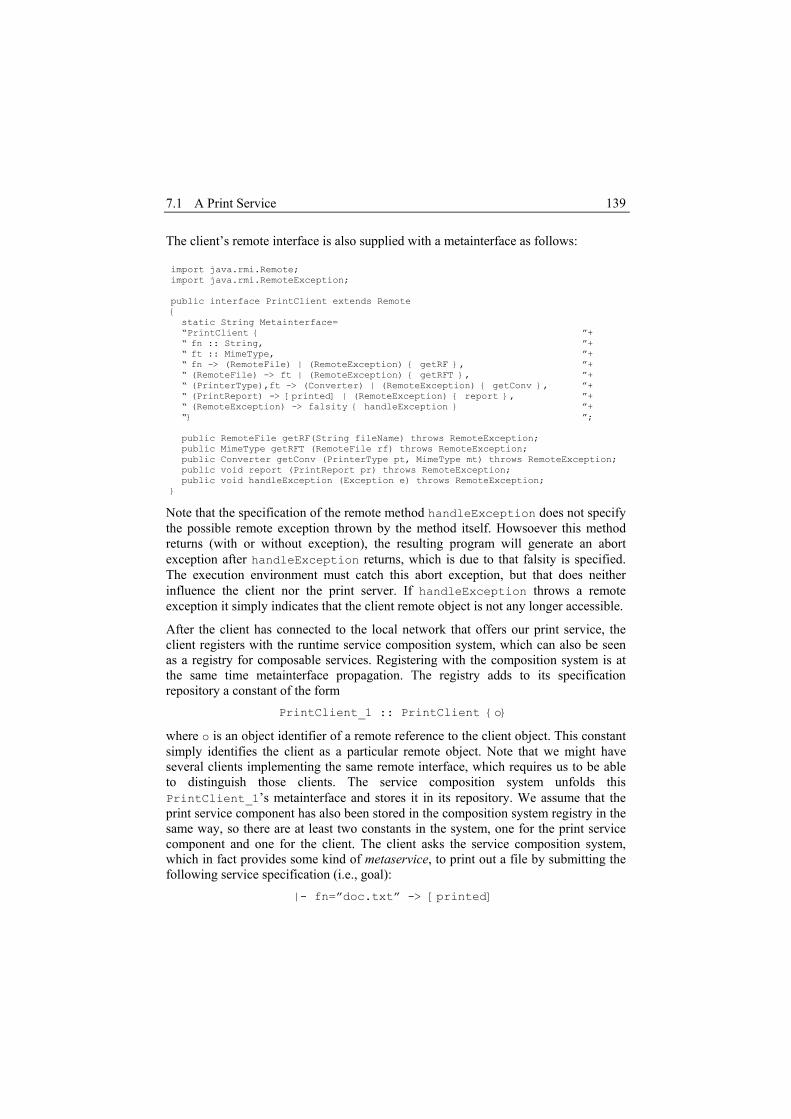
7.1 A Print Service 139
The client’s remote interface is also supplied with a metainterface as follows:
import java.rmi.Remote; import java.rmi.RemoteException; public interface PrintClient extends Remote { static String Metainterface= “PrintClient { ”+ “ fn :: String, ”+ “ ft :: MimeType, ”+ “ fn -> (RemoteFile) | (RemoteException) { getRF }, ”+ “ (RemoteFile) -> ft | (RemoteException) { getRFT }, ”+ “ (PrinterType),ft -> (Converter) | (RemoteException) { getConv }, ”+ “ (PrintReport) -> [printed] | (RemoteException) { report }, ”+ “ (RemoteException) -> falsity { handleException } ”+ “} ”; public RemoteFile getRF(String fileName) throws RemoteException; public MimeType getRFT (RemoteFile rf) throws RemoteException; public Converter getConv (PrinterType pt, MimeType mt) throws RemoteException; public void report (PrintReport pr) throws RemoteException; public void handleException (Exception e) throws RemoteException; }
Note that the specification of the remote method handleException does not specify the possible remote exception thrown by the method itself. Howsoever this method returns (with or without exception), the resulting program will generate an abort exception after handleException returns, which is due to that falsity is specified. The execution environment must catch this abort exception, but that does neither influence the client nor the print server. If handleException throws a remote exception it simply indicates that the client remote object is not any longer accessible.
After the client has connected to the local network that offers our print service, the client registers with the runtime service composition system, which can also be seen as a registry for composable services. Registering with the composition system is at the same time metainterface propagation. The registry adds to its specification repository a constant of the form
PrintClient_1 :: PrintClient {o}
where o is an object identifier of a remote reference to the client object. This constant simply identifies the client as a particular remote object. Note that we might have several clients implementing the same remote interface, which requires us to be able to distinguish those clients. The service composition system unfolds this PrintClient_1’s metainterface and stores it in its repository. We assume that the print service component has also been stored in the composition system registry in the same way, so there are at least two constants in the system, one for the print service component and one for the client. The client asks the service composition system, which in fact provides some kind of metaservice, to print out a file by submitting the following service specification (i.e., goal):
|- fn=”doc.txt” -> [printed]

Chapter 7 Application to Runtime Service Composition 140
The binding fn=”doc.txt” replaces the formal input parameter fn of the service program with the concrete parameter ”doc.txt”.
The realization of this service specification results in a distributed Java program involving two remote objects. The program code shown below is optimized in terms of unnecessary switch-case statements.
class Subtask_1 implements Subtask { PrintClient PrintClient_1 = null; PrintServer PrintServer_1 = null; String PrintClient_1_fn = null; public void subtask(Object[] in, Object[] out) throws AbortException { PrintClient_1_fn = (String)in[0]; Object o = null; try { MimeType PrintClient_1_ft = PrintClient_1.getRFT(PrintClient_1.getRF(PrintClient_1_fn)); Printable PrintServer_1_o = PrintServer_1.convert ( PrintClient_1.getRF(PrintClient_1_fn), PrintClient_1.getConv ( PrintServer_1.getPT(), PrintClient_1_ft ) ); PrintClient_1.report(PrintServer_1.print(PrintServer_1_o)); o = Void.TYPE; } catch (java.rmi.RemoteException e) { o = e; } switch (((Class)o == Void.TYPE) ? 0 : 1) { case 0: return; case 1: PrintClient_1.handleException((java.rmi.RemoteException)o); throw new AbortException(o); } } }
Figure 16 Java program to illustrate the print service
To execute the synthesized print service, the execution environment could use the Java reflection tools. The actual program code could look like the following:

7.1 A Print Service 141
... String srvProgClassName = (1) synthesize(inputParams, outputParam); if (srvProgClassName == null) { // Tell client that service not possible ... return; } try { // Create an instance of the synthesized service Class c = Class.forName(srvProgClassName); (2) Object o = c.newInstance(); // Initialize remote objects for (int i=0; i<numOfRemoteObjects; i++) { (3) Field f = c.getDeclaredField(remoteObjects[i]); f.set(o, remoteObjectRefs[i]); } // Collect service program parameters Object[] subtaskParams = new Object[numOfParams]; for (int i=0; i<numOfParams; i++) { (4) Field f = c.getDeclaredField(inputParams[i]); if (f.getType() == Class.forName("java.lang.String")) { subtaskParams[i] = params[i]; } else if (...) { : } } // Execute the synthesized service program Class[] parameterTypes = new Class[2]; parameterTypes[0] = (new Object[0]).getClass(); parameterTypes[1] = parameterTypes[0]; Method m = c.getDeclaredMethod(“subtask”, parameterTypes); Object[] args = new Object[2]; args[0] = subtaskParams; args[1] = new Object[1]; m.invoke(o, args); (5) } catch (Exception e) { // Tell client that service not possible ... return; } ...
Figure 17 Java program that uses the synthesized print service
Five steps are needed to synthesize distributed services if we use Java RMI. The first step is to synthesize the requested service program (1). The synthesizer returns the name of the class that realizes this service. Second, we create a fresh instance of the generated Java class (2); third, we initialize the remote objects (3), i.e., the constants PrintClient_1 and PrintServer_1 that are involved in the distributed service program; fourth, all service parameters need to be collected (4); and fifth, we execute the service (4).

Chapter 7 Application to Runtime Service Composition 142
The node at which this service program has been composed executes it while the remote methods of the print server component and client component are executed at their respective network nodes. Clients and print servers may differ in their metainterfaces; hence, different service programs can be generated for the same service, depending on the client’s and server’s metainterface. This yields high flexibility in the sense that a client is not bound to a particular server implementation and a server can adapt to any client’s needs, provided the metainterfaces of the server and client allow it. This implies that any component involved can be changed in any way, as long as the modified metainterface preserves computational information with respect to the substituted component. This allows us to remove, modify, and add components in a running system. For this example we could think that a real implementation would also involve components for security, authentication, billing, and perhaps monitoring. Since all those service components are loosely connected through their respective metainterfaces we can easily replace them. This shows the advantage of using declarative programming for services instead of the traditional, imperative approach.
7.2 Stock Quote Cache
The stock quote cache, which we have conceptually already described in section 2.5, is a typical application of runtime service composition to provide fully automatically reconfigurable active network nodes.
Obtaining stock quotes via the Internet is popular. Fast access to up-to-date quotes even during periods of heavy server load is crucial. However, web caches do not help in this context because, first, stock quotes are dynamic data that is usually not cached, and second, the granularity of objects stored in web caches is inappropriate for this application. Typically, clients request a web page that contains a short customized list of quotes but considering hundreds of stocks, the number of possible web pages is huge. Hence, the probability of cache hits is very low.
Active networks allow tailoring caching strategies to suit the application needs. Assume we want to implement a customized protocol for accessing stock quotes, which also allows implementing a reasonable caching strategy at an interior node in an active network. Assume some node of our active network implements a web cache, which does not cache dynamic data. We can model this web cache by a main component and a cache component. The main component, which is configured with the cache component, processes the HTTP request and does the cache lookup. On a cache hit, it sends the response. On a cache miss, the HTTP request will be forwarded to the corresponding server. The basic idea is that web pages and stock quotes are cached at network nodes as they travel from the server to a client.
We use four metaclasses to illustrate this example in Java. We assume that for every stock quote or HTTP request an instance of the composed service program is created

7.2 Stock Quote Cache 143
by the active network node and executed within a thread, as usual for request handlers.
Initially the active network node uses only two metaclasses, which are HTTPRequest and Cache. These two classes provide a cache for any web content identified by a url. The metaclasses are as follows:
class HTTPRequest extends Request { static String Metainterface= “HTTPRequest { ”+ “ url :: String, content :: byte[], ”+ “ httpCache :: Cache {Node.cache}, ”+ “ httpCache.key = url, httpCache.data = content, ”+ “ [url -> content] -> (FwdResp) { handleHTTPRequest } ”+ “} ”; public FwdResp handleHTTPRequest (Subtask cache) {...} }
Class Cache { static String Metainterface= “Cache { ”+ “ key :: Object, data :: byte[], ”+ “ key -> data { lookup } ”+ “} ”; public synchronized byte[] lookup (Object key) {...} }
The actual cache is provided by the network node (Node.cache), which is specified by the constant httpCache. For any instance of the class HTTPRequest, the method handleHTTPRequest either forwards this request (if the corresponding content could not be found in the cache) or sends a response (if the requested object was in the cache). In order to handle requests that use different protocols we need an additional protocol filter. We also need a specialized handler for stock quote requests. The additional metaclasses are as follows:
class StockQuoteRequest extends Request { static String Metainterface= “StockQuoteRequest { ”+ “ share :: String, quote :: byte[], ”+ “ stkQtCache :: Cache {Node.cache}, ”+ “ stkQtCache.key = share, stkQtCache.data = quote, ”+ “ [share -> quote], [QtFmt |- stkq -> html] -> ”+ “ (FwdResp) { handleStkQtRequest } ”+ “} ”; public FwdResp handleStkQtRequest (Subtask cache, Subtask toHTML) {...} }

Chapter 7 Application to Runtime Service Composition 144
class ProtocolFilter { static String Metainterface= “ProtocolFilter { ”+ “ (Socket) -> (HTTPRequest) | (StockQuoteRequest) { filter } ”+ “} ”; public static Request filter (Socket client) {...} }
The metaclass StockQuoteRequest deploys the same cache (provided by the system) as the HTTP-request handler class. The method handleStkQtRequest uses the independent subtask QtFmt|-stkq->html to format stock quote data obtained from the cache into a proper format for display by clients. We do not specify the class QtFmt.
The class ProtocolFilter provides a class method filter that receives as input a reference to an instance of class Socket and returns a reference to an instance of class HTTPRequest or StockQuoteRequest, depending on the request read from the socket. Note that the method filter returns an object of class Request, where the specification of method filter declares that either an HTTPRequest object or StockQuoteRequest object is returned, and the classes HTTPRequest and StockQuoteRequest both extend Request. We use this polymorphism to distinguish between requests using different protocols. This is another way of using disjunction in specifications, but this works only as long as specified outputs have distinct data types.
After uploading the additional metaclasses to the respective network node we force this network node to reconfigure itself, i.e., to compose a new cache service to provide cache functionality for both HTTP and stock quote requests, by stating the goal:
ProtocolFilter |- (Socket) -> (FwdResp)
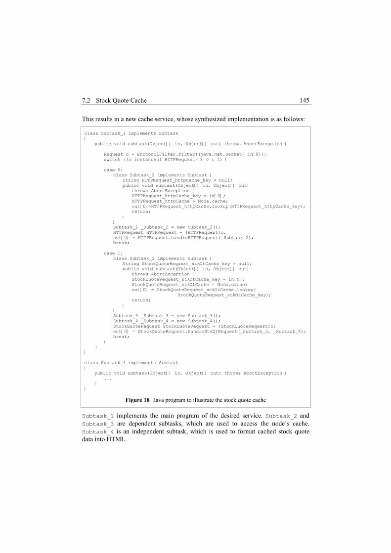
7.2 Stock Quote Cache 145
This results in a new cache service, whose synthesized implementation is as follows:
class Subtask_1 implements Subtask { public void subtask(Object[] in, Object[] out) throws AbortException { Request o = ProtocolFilter.filter((java.net.Socket) in[0]); switch ((o instanceof HTTPRequest) ? 0 : 1) { case 0: class Subtask_2 implements Subtask { String HTTPRequest_httpCache_key = null; public void subtask(Object[] in, Object[] out) throws AbortException { HTTPRequest_httpCache_key = in[0]; HTTPRequest_httpCache = Node.cache; out[0]=HTTPRequest_httpCache.lookup(HTTPRequest_httpCache_key); return; } } Subtask_2 _Subtask_2 = new Subtask_2(); HTTPRequest HTTPRequest = (HTTPRequest)o; out[0] = HTTPRequest.handleHTTPRequest(_Subtask_2); break; case 1: class Subtask_3 implements Subtask { String StockQuoteRequest_stkOtCache_key = null; public void subtask(Object[] in, Object[] out) throws AbortException { StockQuoteRequest_stkOtCache_key = in[0]; StockQuoteRequest_stkOtCache = Node.cache; out[0] = StockQuoteRequest_stkOtCache.lookup( StockQuoteRequest_stkOtCache_key); return; } } Subtask_3 _Subtask_3 = new Subtask_3(); Subtask_4 _Subtask_4 = new Subtask_4(); StockQuoteRequest StockQuoteRequest = (StockQuoteRequest)o; out[0] = StockQuoteRequest.handleStkQtRequest(_Subtask_3, _Subtask_4); break; } } } class Subtask_4 implements Subtask { public void subtask(Object[] in, Object[] out) throws AbortException { ... } }
Figure 18 Java program to illustrate the stock quote cache
Subtask_1 implements the main program of the desired service. Subtask_2 and Subtask_3 are dependent subtasks, which are used to access the node’s cache. Subtask_4 is an independent subtask, which is used to format cached stock quote data into HTML.

Chapter 7 Application to Runtime Service Composition 146
7.3 Summary
In this chapter we have described two examples of the application of our program synthesis method to service composition. The print service example is typical for ad-hoc services in mobile networks where service composition takes place for any given service request. The stock quote cache service is an example for providing flexibility in active networks. Our composition method provides fully automatic network node reconfiguration; however, the reconfiguration frequency is typical low.
Our proposed service composition method is domain-independent and therefore finds its applications in many service domains, not necessarily only network services. The limitation of our approach to fully automatic service composition lays in its restriction to services that possess an uninterrupted chain of dataflow.

Chap t e r 8
Concurrent Implementation of Synthesized Services
A structurally synthesized program does not have any constraints on its execution order other than those imposed by the data dependencies and logical constraints explicitly expressed in the pre- and postconditions of the computability statements. Viewed the other way around, a program’s specification contains explicit and easily usable information about all data dependencies that must be taken into account when synchronizing the concurrent execution of its parts. This can be used for parallelization of structurally synthesized programs. Still, the existing implementations of the structural synthesis of programs (SSP) produce code only for sequential execution in a single thread, although the first paper on concurrent execution of programs obtained by structural synthesis appeared long ago (Plaks 1977). Also the parallel computing models developed and investigated in (Malyshkin 1983) were quite close to the specifications for SSP, and could have been used for introducing concurrency into structurally synthesized programs. The ideas from (Malyshkin 1983) were to some extent used in the packages developed for parallel processing on the NUTS platform (Vlassov, Addibpour, and Tyugu 1998).
At present we have a new implementation of the extended structural synthesis of Java programs that supports both multithreading and an easy way to organize concurrent computations in a network of workstations. Consequently, technically good possibilities exist, both for using fine-grained and coarse-grained concurrency in the
147

Chapter 8 Concurrent Implementation of Synthesized Services 148
implementation of structurally synthesized algorithms. The question answered in this chapter is how to parallelize computations automatically, which is needed for programs synthesized dynamically at run-time. First, we discuss synthesis of concurrent programs using dataflow synchronization in general; second, we consider a multithreaded implementation of structurally synthesized algorithms in Java. Finally, we discuss strategies for coarse-grained parallelization on the basis of the information available in the specifications for ESSP under the assumption that no help for parallelization can be expected at run-time from the user.
8.1 Multithreaded Execution of a Synthesized Program
Our synthesis method uses a constructive logic that allows us to specify dataflow among pre-programmed modules. Let us consider the following example where the input for synthesis is given as a set of computability statements (in LL, see 3.3.1) that includes among others the following three formulae: f:A⊃B, g:U⊃V, and h:B∧V⊃X, where A⊃B, U⊃V, and B∧V⊃X are specifications of pre-programmed modules f, g, and h, respectively. The propositional variables A, B, U, V, and X are types that express the conceptual roles that their respective values play in computations. The dataflow between f, g, and h is then described by their respective specifications, i.e., the output of f (which is specified by B) and the output of g (specified by V) are used as inputs for h.
Conventional implementations of the SSP extract an algorithm from a proof, which is then translated into byte code (Tyugu, Matskin, and Penjam 1999) or source code of a particular target programming language (Lämmermann 2000). In either case, the resulting program is executed sequentially in a single thread. The following figure sketches the synthesis process of a sequential program for computing an object specified by X from objects specified by A and U.
:: : : :: ( ) : : ( ) :
: , : ( ( ), ( )) :. ( ( ), ( )) :
f A B g U Va A a A u U u Ua A f a B u U g u V
a A u U h f a g u Xau h f a g u A U Xλ
⊃ ⊃
∧ ⊃
0 00 000 0
00
Proof:
::h B V X∧ ⊃
Sequential program: func (a, u) begin return(h(f(a), g(u));end
Algorithm extraction: 4) apply f on a A 5) apply g on a U 6) apply h on the
result of f and g
Theory: : f:A⊃B g:U⊃V h:B∧V⊃X
Figure 19 Steps of conventional structural synthesis of programs

8.1 Multithreaded Execution of a Synthesized Program 149
A concurrent implementation of a structurally synthesized algorithm is constructed of a set of dynamically created guarded threads and shared input/output objects that are used for communication between guarded threads. A guarded thread represents a function selected from the proof of the existence of the result. Shared input/output objects are available to the guarded threads through an environment. The shared objects serve as "communication channels" for passing the result of one function (thread) to other functions (other threads). As in the dataflow computation model, a guarded thread can perform its computations if the input objects required in the computation exist, i.e., if the thread can get an input object and operate on it when needed. If a required input object is not available yet (i.e., if it has not been bound yet), the thread is suspended while waiting for the input object to be bound. This computation model is similar to distributed Oz (Van Roy et al. 1997). When the thread completes, it binds its computation result to its output object. It may happen that the output object still contains the result bound by a previous instance of the thread, i.e., the output object was not yet consumed by another thread. In dataflow, such situation is called a data collision (or a collision of tokens that represent the data). The simplest way to avoid data collisions is to suspend the thread that tries to bind its computation result to its respective output object until the output object can be reused for binding the computation result. This approach requires maintaining a queue of threads suspended on the shared object that cannot be reused. We use a more efficient mechanism to avoid data collisions, which is known as dynamic dataflow. Every instance of one and the same guarded thread is associated with a different instance of the environment. Every environment creates its own input/output objects. A guarded thread knows only those objects that are needed for input and output. A shared object can be considered as a "write-once" (or "bound-once") object.
A guarded thread proceeds as follows: 1) it waits until all objects needed as inputs become available, 2) then it executes, and 3) it binds its computation result to its respective output object. Let us assume that we have a programming platform with some means to realize dataflow synchronization, i.e., waiting for input values. A simple synchronization approach is to use dynamic dataflow synchronization for guarded threads that represent separately every function extracted from the proof. In this way we construct a concurrent implementation of a structurally synthesized program, where each computational step (i.e., execution of one function) is encapsulated in a separate thread; this is illustrated in the following figure.

Chapter 8 Concurrent Implementation of Synthesized Services 150
: :: : : ::: ( ) : : ( ) :
: , : ( ( ), ( )) :. ( ( ), ( )) :
f A B g U Va A a A u U u Uh B V Xa A f a B u U g u V
a A u U h f a g u Xau h f a g u A U Xλ
⊃ ⊃∧ ⊃
∧ ⊃
0 00 000 0
00
Execution Environment
Thread 3 get b from B, get v from V exec(h(b,v)) bind result h(b.v) to X
Thread 2 get u from U exec(g(u)) bind result g(u) to V
X V
U A
B
Thread 1 get a from A exec(f(a)) bind result f(a) to B
Function selection:select f, select g, select h
Proof:
Theory: f:A⊃B g:U⊃V h:B∧V⊃X
Figure 20 Steps of structural program synthesis using guarded threads
Due to dataflow synchronization (wait until an object is bound) thread 1 and 2 will run in parallel and thread 3 must wait until both threads 1 and 2 have finished their computation, i.e., have bound their outputs to the respective objects.
8.2 Implementation in Java
In this section we discuss the concurrent implementation of structurally synthesized programs in Java. Although Java is not designed for massively concurrent programming, we are still able to implement concurrent applications in Java. It supports threads and provides synchronization primitives that can be used to implement dataflow synchronization. We are well aware that there are other programming languages that do better in terms of concurrent programming, for example the Mozart system (Haridi and Van Roy 1999), which implements the programming language Oz. Oz possesses a built-in dataflow synchronization mechanism (Van Roy et al. 1997). However, we will do with Java, since in this section we rather focus on how to give structurally synthesized programs a concurrent implementation than discussing programming language features; here, the programming language playes a secondary role.
There are several ways to implement concurrent programs of structurally synthesized algorithms. For simplicity, and to keep our examples more comprehensible, we will use easily understandable pseudo-code. In the above example, we assume that the pre-programmed modules f, g, and h are methods of some class. Their internal structure is uninteresting for us. Let us now explain how we implement dataflow synchronization in Java. Recall that data dependencies among methods are expressed by propositional variables of the respective specifications of the methods under consideration. For example, the method h depends on the method f and g specified by their common propositional variables B and V, where B and V occur in the premise of the specification of h and B

8.2 Implementation in Java 151
(respectively V) occurs in the conclusion of the specification of method f (respectively g). In Java, the propositional variables of specifications become instance attributes; they are used as method parameters in extracted programs either as input (if they occur on the left-hand side of the method specification) or as output (if they occur on the right-hand side of the method specification). To implement dataflow synchronization we simply encapsulate an input/output object in a wrapper object, which is an instance of the ObjectWrapper class. The ObjectWrapper class defines two methods, get and bind. Guarded threads use the method get to obtain an input object, and they use the method bind to bind their respective function result to the respective wrapper object. If a guarded thread invokes the method get on a wrapper object then this thread is blocked in the method call of get if the wrapper object has not yet been bound to an object, i.e., the method bind has not yet been invoked on this wrapper object. As soon as the method bind is invoked on this wrapper object, all guarded threads that are blocked in get on this object will execute again. A guarded thread is implemented simply as a class that encapsulates the execution of a method. It invokes the method get on all wrapper objects that wrap the input objects of the encapsulated method, and invokes bind on that wrapper object that wraps the output object of the encapsulated method. The following code example illustrates an implementation of the guarded thread class that encapsulates the method f.
class GuardedThread_f extends Thread { private Subtask_1 env; GuardedThread_f (Subtask_1 env, int id) { super("Guarded Thread ID: [" + id + "]"); this.env = env; this.start();6 } void run() { // get the value of A Object o = this.env.A.get();
// execute the method f and bind the result to B this.env.B.bind(this.env.f(o)); } }
6 There are two ways to create a new thread of execution in Java. One is to declare a class to be
a subclass of Thread. This subclass should override the run method of class Thread. An instance of the subclass can then be allocated and started. Executing the start method of
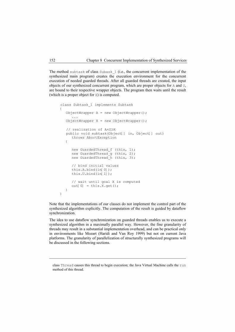
Chapter 8 Concurrent Implementation of Synthesized Services 152
The method subtask of class Subask_1 (i.e., the concurrent implementation of the synthesized main program) creates the execution environment for the concurrent execution of needed guarded threads. After all guarded threads are created, the input objects of our synthesized concurrent program, which are proper objects for A and U, are bound to their respective wrapper objects. The program then waits until the result (which is a proper object for X) is computed.
class Subtask_1 implements Subtask { ObjectWrapper A = new ObjectWrapper(); ... ObjectWrapper X = new ObjectWrapper(); // realization of A∧U⊃X public void subtask(Object[] in, Object[] out) throws AbortException { new GuardedThread_f (this, 1); new GuardedThread_g (this, 2); new GuardedThread_h (this, 3); // bind initial values this.A.bind(in[0]); this.U.bind(in[1]);
// wait until goal X is computed out[0] = this.X.get(); } }
Note that the implementations of our classes do not implement the control part of the synthesized algorithm explicitly. The computation of the result is guided by dataflow synchronization.
The idea to use dataflow synchronization on guarded threads enables us to execute a synthesized algorithm in a maximally parallel way. However, the fine granularity of threads may result in a substantial implementation overhead, and can be practical only in environments like Mozart (Haridi and Van Roy 1999) but not on current Java platforms. The granularity of parallelization of structurally synthesized programs will be discussed in the following sections.
class Thread causes this thread to begin execution; the Java Virtual Machine calls the run method of this thread.

8.3 Coarse-Grained Parallelization 153
The ESSP uses a logic that is much more expressive than the one we used here in our example, specifying subtasks for instance. Imposing parallelism on subtasks is another source for giving structurally synthesized algorithms concurrent implementations. It is possible to implement subtasks as threads as well. The fact that a subtask (which implements a synthesized branch) can be a thread gives us the possibility to execute concurrently several instances of the same subtask. Imposing parallelism on subtasks will be discussed in section 8.3.2.
8.3 Coarse-Grained Parallelization
An obvious way to decrease the execution overhead for each method is to put several methods into the same thread, i.e., to increase the granularity of threads. Some experience with coarse-grained parallelization of synthesized programs exists already. In (Tyugu, Matskin, and Penjam 1999), programs for large simulation problems have been synthesized and run on a network of workstations where parallelism of subtasks has to be pre-programmed in the modules that use subtasks. Here, we will discuss the following two cases with the aim of using the coarse-grained parallelization completely automatically: 1) composing threads, and 2) imposing parallelism on subtasks.
We will use a representation of a structurally synthesized program in the form of a higher-order dataflow scheme (HODS) (Tyugu 1991a). The nodes of a HODS are either functional nodes or control nodes. Figure 21 shows such a scheme with four functional nodes b, c, d and e, and a control node a with one subtask Q. As usual for the SSP, we denote data dependencies as going in the direction of dataflow, showing explicitly also the data items as nodes of the scheme. We use lower-case letters for representing data items. The control nodes not only exercise control over the execution order of synthesized branches, but perform computations as well.
s
v
u
b
dc
Q z
w
t
e
x a y
Figure 21 Higher-order dataflow schema

Chapter 8 Concurrent Implementation of Synthesized Services 154
The scheme shows an algorithm for computing y from x by performing computations under the control of the node a. This node uses a subtask Q for computing z from u and v, possibly repeatedly. When computing the subtask, two branches, b and c;d can be performed concurrently. Parallelization is also possible for the subtasks: depending on the data dependencies in the node a, it may be possible to arrange the computations for each set of values of u and v (repeating computations for the subtask Q) concurrently. How much should be done concurrently, and what should be done at one site, depends on the properties of computations for each functional node. Any attempt to find an optimal solution leads to NP-complete problems. Given the large size of schemes we are handling in SSP (up to thousands of nodes), looking for optimal solutions is implausible. Therefore we consider the following heuristic techniques.
8.3.1 Composing Threads We build threads in order to execute them concurrently by looking for maximal sequences of steps that can be performed sequentially in one thread. A functional node in HODS may have several inputs, like the node a in Figure 22. Therefore it may be included in different threads (Plaks 1977). We have decided to compose threads in such a way that a thread can run without synchronization with other threads after its execution has started (i.e., the synchronization is needed only for starting a thread). Therefore, a node with input from more than one thread (like the node a in Figure 22) will be always the first in a thread.
......
... ...Thread 3
Thread 2
Thread 1
a
Figure 22 Composing threads
8.3.2 Imposing Parallelism on Subtasks Control nodes can easily be implemented in Java in a multithreaded way. Knowing the usage of a control node it may be possible to decide in advance whether its subtasks should be executed concurrently. It is also possible to include into a specification several control nodes, which differ only by their implementation, and to use extra variables in the specification to show which implementation (sequential or concurrent) is needed in a particular case.

8.4 Summary 155
A rich set of control nodes for concurrent execution was developed for the distributed computing platform NUTS that has been described in (Vlassov, Addibpour, and Tyugu 1998). Here we give an example of a control node for parallel processing of collections that implement the Java Enumeration interface (see Figure 23 below). A collection a is processed element by element, each time processing an element x of the collection and computing a new element y of the resulting array c. The subtask P specifies what has to be done with an element x from the collection a in order to get an element of the array c. It is assumed that the subtask P is computationally expensive, and the computations for elements of the collection are performed in parallel.
x y
P
ca
Parallel execution of P
Figure 23 Parallelism in control node
8.4 Summary
In this chapter we have shown how to use the information already existing in a specification for the concurrent implementation of a synthesized program. We have discussed several approaches: multithreaded execution of functions, parallel execution of composed threads, and distributed implementation of a coarse grained concurrent program.
The proposed method offers three advantages. First, it achieves concurrency without requesting additional information from a user. Second, it requires only a comparatively small implementation effort. Third, a composed program does not implement the control part of the synthesized algorithm explicitly but the computation of the program's result is guided by dataflow synchronization. However, the computational overhead implementing fine-grained parallelism may be high if pre-programmed functions are small. In this case, composing guarded threads should be considered.


Chap t e r 9
Related Work
This chapter surveys briefly published work that bears a relation to our work. The survey is divided into three subsections. We start with related work on program synthesis in general before we focus on deductive program synthesis. Thereafter we discuss software composition languages, where we focus on coordination languages and scripting languages. Coordination languages are used to configure applications from distributed, computational components with focus on communication, whereas scripting languages are used to configure applications from components with focus on application composition. Finally, we discuss frameworks for developing network-centric applications by dynamic composition of services.
9.1 Program Synthesis
Program synthesis is a method of software engineering used to generate programs automatically. There are three different approaches to program synthesis. These are transformational, inductive, and deductive program synthesis. In transformational program synthesis, programs are constructed by means of rewriting formal specifications until the logical specifications can be executed as a program. Inductive program synthesis derives programs from input/output examples. Logically, this method makes use of inductive inference, where a general rule is hypothesized from given input/output examples. This hypothesized general rule then gives the program.
157

Chapter 9 Related Work 158
In deductive program synthesis, automated deduction techniques are exploit to construct programs automatically. Deductive techniques use a program's specification that represents a relationship between a given input and the desired output, expressed as a logical sentence. Such a specification can be phrased as a theorem that states the existence of an output that meets the specified conditions. This theorem is proved automatically. The generated proof becomes the basis for a program that can be extracted from the proof.
The following two subsections only survey briefly transformational and inductive program synthesis. We discuss deductive program synthesis more deeply in section 9.2.
9.1.1 Transformational Approach A wide variety of programming systems make use of program transformations. In (Darlington 1986) transformations are used to automatically improve the efficiency of a program. The system operates by applying a number of transformations to merge information from different parts of the input program and then to redistribute it into a more efficient program, which is the output of the system. Another use of transformations is to define higher-level programming constructs in terms of lower-level constructs, or on the level of formal specifications, as mentioned above, rewriting formal specifications until the logical specifications can be directly translated into a programming language. However, it is important to verify that the transformations are correctness preserving. In other words, the transformation process must not alter the intended behavior of a program. Broy and Pepper discuss in (Broy and Pepper 1986) the semantic foundations necessary to support this kind of verification.
To get an impression of transformational program synthesis we give a small example, the natural number approximation of dual logarithm. The specification of the problem is as follows:
: | : 0. : . 2 2 yf Nat Nat n Nat n y Nat n n→ ∀ ∧ > ∃ ÷ < ≤
From this specification we know: f(n) ≤ log2(n) and n>0. According to the laws of logarithm we know also log2(1) = 0. We have to consider two cases:
2
2 2
1, (1) log (1) 01, ( ) log ( ) log ( 2) 1 ( 2) 1
n then fn then f n n n f n
= ≤ => ≤ = ÷ + = ÷ +
The rewritten specification can be directly translated into the recursive program:
:( ) 1 0 ( 2) 1
f Nat Natf n if n then else f n fi
→≡ = ÷ +
A major problem in transformational program synthesis is choosing which transformation rule to apply next if several rules are applicable; this often requires

9.1 Program Synthesis 159
user interaction. It is also possible to search all possible transformational paths, creating a variety of output programs, as for example implemented in the PECOS system (Barstow 1986).
9.1.2 Inductive Approach In the literature, inductive program synthesis is often referred as programming by example. Programming by example systems seek to synthesize programs based on examples of their behavior. In a number of simple situations programming by example has been successfully demonstrated but its methods do not scale up effectively to programs of realistic complexity and size.
Fundamental theoretical results on which most programming by example systems are based are presented in (Summers 1986). To illustrate the basic idea of programming by examples, we consider the problem of generating the function head[x]. The program’s task is to extract the first element of a nonempty list x. We will use the programming language LISP (Allen 1980). We assume that the reader is familiar with LISP basics even though the used LISP code fragments are self-explanatory. A set of input/output examples that might be given as program specification is:
{( ) ( ),( ) ( ),( ) (
A AA B A
)}A B C A
→→
→
Each example represents a transformation that is then encoded in a function. The functions are compositions of the primitive functions car and cons, which can be derived algorithmically (Summers 1986). From the examples above we can derive three functions:
1
2
3
[ ] [ [ ]; ];[ ] [ [ ]; ];[ ] [ [ ]; ];
f x cons car x nilf x cons car x nilf x cons car x nil
==
=
From f1, f2, and f3 we hypothesize the general rule:
1
1
[ ] [ [ ]; ];[ ] ; 1i i
f x cons car x nilf x f i+
== ≥
.
From the hypothesized rule we extract the final LISP program:
[ ] [ [ ]; ]head x cons car x nil← .
Generalizing program specifications from examples of behavior is the key problem in programming by examples. Creating a program that supports only given input/output examples is trivial. But it is the goal to create a program that can operate on a whole class of data in a way that is analogous to the examples. Often the assumption is made that examples are given in such a way that the simplest program satisfying the

Chapter 9 Related Work 160
examples is correct (Muggleton ed. 1997). Therefore, the inductive approach offers no correctness guarantee for a program that should operate on a whole class of data.
9.2 Deductive Program Synthesis
Deductive program synthesis is based on the observation that proofs are equivalent to programs because each step of a proof can be interpreted as a step of a computation. This transforms program synthesis into a theorem-proving task. The key ideas of this approach, namely the correspondence between theorems and specifications and between constructive proofs and programs are presented in (Manna and Waldinger 1992).
The difference between a constructive and nonconstructive proof is that a constructive proof shows the existence of an object by supplying a method for computing the object's value, where a nonconstructive proof shows only the existence of an object but leaves its value unknown.
Deductive program synthesis has been studied for many years and has been used in practice for developing industrial software. It is based on the observation that constructive proofs are equivalent to programs (Howard 1980), because each step of a constructive proof can be interpreted as a step of computation. This observation is also known in the literature as the “Curry-Howard isomorphism”, the “proofs as programs paradigm”, or the “formulae as types interpretation”. There are many approaches to deductive program synthesis (Rich and Waters 1986). Though those deductive systems are different, most systems use constructive or constructively restricted theorem provers to derive a program from its specification.
This subsection identifies important work on this subject. We discuss the fundamental method of deductive program synthesis and describe briefly some deductive program synthesis systems: KIDS, Planware, Amphion, and NUT. We compare the NUT and Amphion systems, which are the closest to our approach.
9.2.1 Deductive Program Synthesis Methods Manna and Waldinger discussed the fundamentals of deductive program synthesis in (Manna and Waldinger 1992) and developed a first-order synthesis methodology that employs the sequent as basic structure (Manna and Waldinger 1986). A sequent consists of two lists, assertions A1, A2, …, Am, and goals G1, G2, …, Gn. Each assertion or goal may be associated with an entry called the output expression, which records the program segment that has been constructed at each stage of the derivation. A sequent is denoted by a two-dimensional structure called a deductive tableau to present a proof state. Each row in the tableau contains three columns: assertions, goals, and outputs. A row of the tableau has the form

9.2 Deductive Program Synthesis 161
assertions goals outputs Ai(a, x) ti(a, x)
or
Gj(a, x) tj(a, x)
The meaning of such a sequent is that if all instances of each of the assertions are true, then some instances of at least one of the goals is true. Hence, the proof process is complete if the tableau contains a final row
true t or, by duality
false t
where t is an expression that implements the desired program.
Synthesis starts with a specification of the desired program. A specification has the form f(a) ⇐ find z such that R(a, z) where P(a)
The initial sequent is thus constructed as follows:
assertions goals outputs f(a)
P(a) R(a, z)
z
The main proof rule is non-clausal resolution, which is different from the original resolution principle by Robinson (Robinson 1965). The original resolution principle requires that sentences must be put in conjunctive normal form, which sometimes results in unmanageable size of the set of clauses. As a result, proofs loose their intuitive content. Non-clausal resolution is similar to a case analysis in program development and is responsible for the introduction of conditional terms in the program. Manna and Waldinger use four versions of non-clausal resolution. The following example, which is taken from (Manna and Waldinger 1986), uses the GG-resolution rule.

Chapter 9 Related Work 162
Suppose we have derived the two goals
assertions goals outputs max(l)
max(tail(l)) ≥ head(l) and tail(l) ≠ []
max(tail(l))
not(max(tail(l)) ≥ head(l)) and tail(l) ≠ []
head(l)
The two goals rows contain two unifiable quantifier-free subsentences, which are: P≡max(tail(l))≥head(l) and P'≡max(tail(l))≥head(l). Then by eliminating the subsentence max(tail(l)) ≥ head(l) via GG-resolution, we can derive the new goal
(true and tail(l) ≠ []) and (not false) and tail(l) ≠ []
if max(tail(l)) ≥ head(l) then max(tail(l)) else head(l)
The new goal or resolvent is a conjunction of both original goals under the image of the unifier θ after replacing all occurrences of P by true and P' by false. The output term is a conditional with Pθ as condition and the two initial terms max(tail(l)) and head(l) as branches.
The calculus also provides auxiliary rules for splitting, transformation, and handling of equivalences. Splitting rules are used to decompose an assertion or goal into its logical components. Transformation rules allow deriving an assertion or goal from another. The calculus includes also a rule for well-founded induction to introduce recursion.
Manna and Waldinger's deductive tableaux approach to program synthesis has been used to derive a wide range of programs. The SNARK system (Stickel et al. 1994), for instance, automates proof search in parts of the framework of (Manna and Waldinger 1986). Deductive tableaux have also been re-interpreted in higher-order logics (Ayari and Basin 2001). There are other approaches to automated program synthesis that try to integrate different techniques into deductive synthesis. For instance, in (Fischer and Whittle 1999) Fischer and Whittle report a study on integration of deductive retrieval into deductive tableaux in order to maximize the advantages of both approaches. Deductive synthesis uses a theorem prover to derive a program from its specification, where deductive retrieval (Penix and Alexander 1999, Schumann and Fischer 1997) is a technique applied by theorem provers, to find existing components for specifications during proof search by querying the retrieval subsystem. Both techniques are complementary. The goal of the integration is to identify proof states where retrieval can be applied, which avoids overloading the retrieval subsystem with an excessive number of redundant queries.
9.2 Deductive Program Synthesis 163
9.2.2 The Amphion System The Amphion system (Lowry et al. 1994) synthesizes programs by composition of existing subroutines. It provides automation of the software development process and improves the productivity and quality of software engineering. In the framework of the Amphion system, methods of automated theorem proving developed by Waldinger are applied to the composition of subroutines into software. In that sense it is similar to the work of Tyugu and others (Tyugu 1988), in which software is also generated from pre-programmed modules (i.e., subroutine libraries), to meet specifications expressed in intuitionistic propositional logic.
Amphion’s first application domain is software for planning and interpreting space-science observations. The software is based on the SPICELIB, a library of procedures for solar-system geometry. In Apmphion, software requirements are specified in a graphical notation. An interactive interface, which is domain-independent but employs the vocabulary of the domain, presents the user with a menu of alternatives and elicits the specification gradually. The graphical specification is automatically translated into a first-order-logic theorem. A program is developed from the logical form of the specification using the automated deduction system SNARK (Stickel et al. 1994). SNARK is especially suitable for program synthesis and other applications in artificial intelligence and software engineering.
9.2.3 The NUT System NUT (Tyugu 1994) is the most recent system in the so-called Priz family of systems (Tyugu 1991b) in which the Structural Synthesis of Programs (SSP) is the central technique. SSP uses intuitionistic propositional logic (Mints 1991). In the NUT system, specifications of classes are used for automatic construction of programs using of the Structural Synthesis of Programs (SSP) method. Aspects of SSP are discussed (Uustalu 1995a). The NUT system demonstrates the feasibility of using a declarative language as a tool for automated implementation of requirements written in a semi-formal manner (Addibpour and Tyugu 1996) and has also been used for program synthesis in a distributed environment described in (Vlassov, Addibpour, and Tyugu 1998). The NUT system has been successfully used for very large and precise hydraulic simulation problems where it has shown very good scalability and synthesis performance (Grossschmidt, Vanaveski, and Harf 2000).
9.2.4 Amphion vs. NUT Both the Amphion system and the NUT system restrict their attention to the construction of programs composed from pre-programmed modules, rather than the primitive instructions of a programming language. In both systems a deductive approach is used to construct programs from proofs. The NUT specification language is an object-oriented language extended with features for program synthesis (Tyugu 1998). In the NUT system pre-programmed modules are methods of classes supplied
Chapter 9 Related Work 164
with specifications (Tyugu 1994). The Amphion system makes use of subroutine libraries as a collection of pre-programmed modules. In the Amphion system, programs are constructed by means of generating source code. In the NUT system, generating an algorithm and encoding it in the byte-code of the NUT virtual machine construct programs.
Amphion and NUT make use of composing programs from pre-programmed modules. However, the nature of these pre-programmed modules is different in both systems. Amphion uses subroutine libraries and NUT makes use of methods of classes. On a high level of abstraction one can say both systems compose programs from components.
9.2.5 KIDS A knowledge-based software development system called KIDS (Kestrel interactive development system) (Smith 1990, 1991) has been developed at the Kestrel Institute. KIDS is a semi-automatic program development system from which the programmer can obtain correct and efficient executable program code through the use of automated tools. The system provides tools for performing deductive inference, algorithm design, partial evaluation, data type refinement, and other transformations. A formal specification is developed into a program by interactively applying a sequence of high-level transformations.
9.2.6 Planware Kestrel’s Planware (Blaine et al. 1998) is an interactive system for generating automatically high-performance schedulers from specifications of scheduling problems. The specification of the scheduling problem is assembled from the planning and scheduling knowledge of experts in this area. Interactions with the system are designed to be entirely in the scheduling domain, i.e. the user does not need to be able to read or write formal specifications. Planware is an extension of the Specware system (Srinivas and Jullig 1995), a system for developing formal specifications and refinements based on concepts from higher-order logic and category theory.
9.3 Software Composition Languages
Components implement abstractions related to a particular problem domain. They are black-boxes entities that both provide and require computation (Achermann et al. 2000). A component can be a function, a class, an application, or even a server. The construction of software applications from components is what we call software composition. Software systems composed from components provide increased

9.3 Software Composition Languages 165
flexibility, because a system built from components can easy be recompiled to address new requirements (Nierstrasz and Dami 1995).
A running system can be described as a collection of interacting objects; this gives the computational view. The specification of the same system can be seen as a composition of software components, which gives the compositional view. The way in which a system is composed must be open to changes, i.e., the system must be recomposable if the requirements change. In (Nierstrasz and Meijler 1994) Nierstrasz and Meijler argue that object-oriented techniques support this view of open systems but fail to distinguish the computational and compositional views of applications, and over-emphasize the object view, thus failing to provide general component specification and composition mechanisms. However, it has been pointed out in (Nierstrasz and Meijler 1995) that software composition can be reduced to one of the following composition models: 1) macro expansion, 2) higher-order functional composition, or 3) binding of communication channels.
A composition language is a combination of an architecture description language, a scripting language, a coordination language, and a glue language. Architecture description languages are used to specify and reason about component architectures and architectural styles (Shaw and Garlan 1996). Scripting languages, such as Perl (Wall, Christiansen, and Schwartz 1996) and Python (Salus 1998), allow specifying applications as configurations of components according to a given architectural style. Coordination languages configure applications from (usually distributed) computational agents, and glue languages allow specifying component adaptation, which is needed because we are often constrained to use legacy components that are not plug-compatible with the components we want to work with. Incompatible components can cause compositional mismatches (Sametinger 1997), which then require component adaptation. Component adaptation is not provided by our approach, because we use a logical specification language. However, there are two possibilities to provide to some extent component adaptation: 1) component adaptation by changing the structural specification of a component if possible, and 2) component adaptation by implementing a component wrapper and using the structural specification of the wrapper component instead of the specification of the wrapped component.
A composition language can be used to specify compositions explicitly, or it can be used for writing a declarative specification of a composition (of a service in our case) so that the latter will be generated automatically. This is our approach where services applications are built based on automatically generated proofs. Similarly, scripting is also implemented as program extraction from proofs.
Supporting dynamic composition of applications from components requires that a component must provide ports or connectors that can be used to connect this component with others (Succi et al. 2000). If a composition involves only connecting ports of components then we talk about coordination. Coordination languages are of particular interest for us because information needed to compose coordinators

Chapter 9 Related Work 166
(software applications that connect components) can be extract from proofs, as explained in Chapter 8.
9.3.1 Coordination Languages Coordination languages are used to manage dependencies between concurrent or distributed components. Managing (dataflow) dependencies in concurrent, even distributed environments, means coordination rather than writing scripts that compose components to software applications. Many coordination languages have been proposed, for instance Linda (Carriero and Gelernter 1989) and Darwin (Magee, Dulay, and Kramer 1992). In this section we discuss the relation of coordination languages to our approach to service composition. In particular, we highlight common properties of coordination in Manifold (Arbab 1996) and the dataflow-based coordination of our composition method.
Important characteristics of computation models on which coordination languages are based, include compositionality, which it inherits from the dataflow model (i.e. dataflow dependencies among components), and separation of computation concerns from communication concerns. The computation model of our method of service composition belongs essentially to the same class.
Traditional concurrent applications, such as client-server solutions, require programmers to deal directly with lower-level communication primitives that comprise the realization of the cooperation model of a concurrent application. Communication primitives are scattered throughout the program code and are mixed with computation primitives, which results in inflexibility and makes those applications hard to reuse (Arbab 1996). Communication involves a sender and a receiver. A sender sends a message to a receiver, where the receiver is either statically known or dynamically evaluated. A receiver typically waits to receive a message (blocking). This communication model encompasses theoretical models such as CCS (Milner 1985).
Consider the following example of a concurrent application. Two processes must cooperate with each other by producing values and passing them to the respective cooperator. The program code of the two processes might look like as follows (we reuse exactly the same example as presented in Arbab 1996):
process p: compute m1 send m1 to q compute m2 send m2 to q do other things receive m do other computation using m
process q: receive m1 let z be the sender of m1 receive m2 compute m using m1 and m2 send m to z

9.3 Software Composition Languages 167
Communication primitives are mixed with computation primitives. If we consider the communication primitives of both processes only, i.e. send and receive, we can recognize an asymmetry between send and receive. The problem with this asymmetry is that both processes make assumptions about their environment, i.e. availability and accessibility of the other process. These assumptions are hard-wired into the program code. Hence, the dependencies of both processes on their environment make them inflexible and hardly reusable if we want them to cooperate with two other processes in a similar fashion.
Coordination languages serve to overcome this problem by allowing writing scripts or programs, called coordinator or manager, with the only purpose to establish communication channels or links between processes such that a process does not send a message to a particular receiver or receive a message from a particular sender. Messages are written to and read from ports. A manager encoded in a coordination language links the ports of processes and thus coordinates communication; in particular, the manager determines sender and receiver, not the processes themselves.
Reconsider our example from above. We now show how it can be implemented using a coordination language. We simply add a third process, the manager that only creates communication channels between the two processes. Send and receive operations of the two original processes have been replaced with write- and read-primitives that operate on ports. process p: compute m1 write m1 to output port o1 compute m2 write m2 to output port o2 do other things read m from input port i1 do other comp. using m
process q: read m1 from input port i1 read m2 from input port i2 compute m using m1 and m2 write m to output port o1
process manager: ... create channel p.o1->q.i1 create channel p.o2->q.i2 create channel q.o1->p.i1 ...
The benefit of using coordination languages lies in the enhanced flexibility and reusability of processes: processes do not need to know where their input comes from, nor do they need to care where their output goes to. They make no assumptions about their environment and contain no communication coordination primitives. Any particular cooperation model is moved into a separate manager process and thus made explicit (Arbab 1996).
Still, this kind of coordination requires knowledge of the internal structure of processes to be coordinated, i.e., we need to know what is computed when and where, and what is needed where and when. For instance, coordination in Manifold requires information available to a coordinator process about the behavior of the processes it coordinates. This comprises a specification of input and output sequences and the

Chapter 9 Related Work 168
relative timing of the events processes may emit and expect. This in turn requires different managers for computationally equivalent processes, i.e. processes that input and output the same values but in different sequences. Our approach to service composition allows another solution. Instead of using specifications of the I/O behavior of processes, we decompose processes into separate components, supply them with structural specifications and synthesize the coordinator process according to dataflow dependencies among components. The limitation of our approach is that we cannot encode in our logic events emitted and expected by components.
There are two interesting properties that are common to coordination in Manifold and the topic of this thesis work. First, coordination in Manifold is based on dynamic dataflow networks; we use dataflow networks as data structures for proof search (see section 3.2.9) and extract information from proofs for building concurrent applications. Second, Manifold allows the decomposition of coordination problems into sub-coordination problems and makes use of so-called manners that are parameterized subprograms. Manners embody coordination of sub-problems. Parameters to a manner can be manifold definitions, processes, events, ports, and other manners. This decomposition is similar to the role of the dependent and independent subtasks of our approach to service composition.
Coordination languages are suitable tools as long as we are concerned only with coordinating communication between (distributed) components. Software composition also requires application configuration and component adaptation by glue code to overcome the problem of components that are not plug-compatible. In the next subsection we briefly discuss a software composition language called PICCOLA, which provides coordination mechanisms, scripting to specify application configuration of components, and supports writing glue code to adapt components.
9.3.2 PICCOLA PICCOLA (Achermann et al. 2000) is a software composition language that enhances flexibility and adaptability needed for component-based applications to handle changing requirements. It supports components, scripts, coordination, and glue code. It follows the requirements for a composition language described in (Nierstrasz and Meijler 1994). Components are understood in the conventional way as black-box entities that both provide and require services. The fact that components may also require service makes them individually configurable, i.e., they can behave differently depending on the supplied service. Scripts are used to specify how components should be plugged together. A script orchestrates an application composition of components by configuring components possibly defined outside the language. Glue code helps to overcome compositional mismatches (Sametinger 1997) by adapting components to the new environment they are used in. By its nature, coordination in PICCOLA is concerned with managing dependencies between concurrent agents, because PICCOLA is based on a process algebra, which is a variant of the π-calculus (Milner, Parrow, and Walker 1992).

9.3 Software Composition Languages 169
The original motivation for developing PICCOLA from a process calculus foundation was to ensure that the interaction of high-level compositional abstractions has a precise semantics in terms of a simple computational model (Achermann et al. 2000). PICCOLA is based on an extension of the asynchronous π-calculus, the πL-calculus. For detailed discussion of the π-calculus and the πL–calculus see (Milner 1990, Lumpe 1999). The formal language of PICCOLA is described in (Lumpe, Acherman, and Nierstrasz 2000). In the πL–calculus the polyadic communication of names or tuples of names is replaced by monadic communication of forms, which is a special notion of extensible records. The approach of the πL–calculus, in which agents communicate by passing forms rather than tuples, addresses the problem that reusability and extensibility of software components is limited due to position-dependent parameters (Achermann et al. 2000).
To highlight the advantages of using monadic communication of forms rather than polyadic communication of names, let us consider an example. We assume that the reader is familiar with basic concepts of the π-calculus. We use the same example as presented in (Achermann et al. 2000). Consider the following expression in the polyadic π-calculus:
! ( , , ).( ')( , , ' | '( , ). , )w a b r v r f a b r r x y r x y⟨ ⟩ ⟨ ⟩
This expression models a process that listens at channel w for a triplet (a,b,r), where a and b are service parameters and r is a channel to which the reply will be sent. If the process receives a message at channel w it creates a private channel r’ and forwards the message to f, which substitutes the reply channel. Another process, started in parallel, picks up the response, and forwards it to the original client along channel r. The important point is that this code hard-wires the protocol. It will not work if the service at channel f extends its interface to accept more (or less) parameters or to return a result with a different arity.
In the πL–calculus, we can encode this example as follows:
! ( ).( ')( ( ' ) | '( ). ( ))replyw X v r f X reply r r Y X Y⟨ = ⟩
The crucial difference is that the service process receives a single form X along w, only assuming that the message received contains a reply channel.
Forms can be complex and even active. Active forms have function or procedure specifications or function calls in place of the simple bindings. This concept allows defining form expressions that can act as objects (Lumpe, Acherman, and Nierstrasz 2000). Hence, it is possible to implement objects in PICCOLA.
Active forms are similar to first-order features of our automated composition method in the sense that they allow to use polymorphic parameters, which we found very important for runtime composition of autonomous components. Still, PICCOLA requires specifying software composition by means of scripts and therefore hard-

Chapter 9 Related Work 170
wires the program to be composed in advance. There is little support for just-in-time composition, i.e., connecting components at runtime according to a specification. However, composition languages such as PICCOLA are needed to specify adaptation and wrapping of components possibly defined outside the language. Apart from the fact that composition in PICCOLA and our approach aim at different usages, they are in our view two complementary and computationally similar techniques. They are complementary in the sense of providing automated composition of abstractions specified in PICCOLA. They are computationally similar because we can describe dataflow networks in both the π–calculus and the calculus of the structural synthesis of programs. The π–calculus encodes dynamic networks (Jagadeesan 1995) which is in contrast to static networks in the structural synthesis of programs. The key idea underlying the π–calculus is the notion of naming: names are used to refer to channels (i.e., the links between processes) and can be dynamically created or hidden, which yields dynamically evolving communication structures among processes. Dataflow networks (Tyugu 1991a) described by structural specifications of the structural synthesis of programs also link processes (i.e., functions) through names of communication channels (i.e., common parameters) but names cannot change dynamically.
The computational similarity and the complementarity of PICCOLA and our approach to software composition make both techniques interesting for just-in-time service composition and consequently a potential source for future work.
9.4 Service Composition
Dynamic composition of services from components is becoming attractive but requires advanced composition models. Interesting work on this subject has been done during the last decade. In particular, during the last years several systems have been proposed to compose services at runtime from components. On one hand this reflects the increasing commercial use of computer networks. On the other hand it shows that due to emerging technologies such as CORBA, Java, and Mozart (Van Roy et al. 1997, Haridi et al. 1998, Haridi and Van Roy 1999) dynamic service composition from components is becoming feasible. Research directions in software composition, such as composition frameworks, architectures, models, languages, methods, and tools have been discussed in (Nierstrasz and Meijler 1995). It has been pointed out that the proposed techniques focus on particular application domains rather than on being a general tool, language, method, or framework for composition. However, it is interesting to observe that many recently proposed approaches to service composition follow the paradigm "Applications = Components + Scripts" (Achermann et al. 2000).
In this subsection we present work related to service composition. Our brief survey, which is subjective and incomplete, is divided into four subsections. We discuss

9.4 Service Composition 171
briefly two very practical approaches to service composition, a commercial system, and present a more detailed discussion on a rule-based system.
9.4.1 A Reuse and Composition Protocol In (Beringer, Wiederhold, and Melloul 1999), a reuse and composition protocol for services is described. It is targeted not on composition and reuse of components or reuse by integrating applications but on composition and reuse of services. In contrast to reusing components, the programs providing services are not moved to the user's site. By using a protocol for reusing remote and autonomous services, a client program is generated, which is based on this protocol.
9.4.2 Hadas Another interesting composition model for dynamic composition of distributed services is described in (Ben Shaul, Gidron, and Holder 1998). It is realized in Hadas (Ben Shaul et al. 1997), a network-centric framework for dynamic composition and deployment of distributed services. It is interesting to see that it focuses also on automatic "just-in-time" deployment, where deployment is carried out as a part of the application composition procedure.
9.4.3 Adaptive and Dynamic Service Composition in eFlow A commercial, dynamic service composition system, called eFlow (developed at Hewlett-Packard Laboratories), is described in (Casati et al. 2000). It supports the specification, enactment, and management of composite e-services modeled as processes. In eFlow, a composite service is described as a process schema that composes other basic or composite services. A composite service is modeled by a graph that defines the order of execution among nodes in the process. Such a graph may include service, decision, and event nodes.
9.4.4 The Aurora Architecture The Aurora architecture (Nikolaou, Marazakis, and Papadakis 1998) is a framework for developing network services by dynamic composition. This architecture complements the CORBA and WWW/Java frameworks with support for coordination and collaboration, and addresses the requirements of dynamic open environments (Marazakis, Papadakis, and Nikolaou 1997) with multiple autonomous service providers. The Aurora architecture provides a run-time environment for a specification language, which is called HERMES.
Th basic concepts of the Aurora architecture are resources, tasks, and events. Resources are software components offering services. As usual, services are accessed via well-defined interfaces. Tasks are activities that use resources. They are defined
Chapter 9 Related Work 172
by the set of required inputs and generated outputs, and a specification of the required resources. Tasks may be compound if they involve multiple resources. Compound tasks are decomposed into a set of interdependent, cooperating tasks. A specification of a compound task determines the communication channels to be established between components. Events are a combination of service request messages, state transition signals, as well as system-generated or application-specific notifications (Marazakis, Papadakis, and Nikolaou 1997). Definitions of resources, tasks, and events are instances of metadata constructs offered by the HERMES language.
The Aurora application model supports a service flow paradigm, where composite services are realized in the context of work sessions as multi-step flows of service requests between components. Control and dataflow is driven by events. Service flow rules, written in the HERMES specification language, are used to define communication channels between software components and actions triggered by events.
HERMES (Marazakis, Papadakis, and Nikolaou 1998) is a specification language that can be used to express scripts for complex activities involving coordination and collaboration. Semantics of service flow rules of the HERMES specification language are defined in terms of causality of application of those rules, i.e. the cause and effect of application of service flow rules, where the cause of application lies in the events considered in the evaluation of the condition of a rule. The general form of a service flow rule is the following:
( ) { }WHEN c Sequence of Actions− − ,
where c is the condition to be evaluated in order to decide whether to execute Sequence-of-Actions. A condition may involve one or more events, combined by boolean operators AND, OR, and NOT. HERMES allows also to define metadata, which are resources, events, and tasks, and associating attribute-value pairs with them.
To give an impression of service flow rules we show a small example, a rule needed for booking tickets used within a travel agent system. We do not show the specifications of the tasks TravelAgent and BookTicketTask. A more detailed discussion of the same example is presented in (Marazakis, Papadakis, and Nikolaou 1998). The service flow rule of this problem is as follows:
WHEN (TravelAgent.START) { TravelAgent.START_PHASE("BookTicket"); BookTicketTask.START [ TravelAgent.Output BECOMES BookTicketTask.Input; BookTicketTask.Output BECOMES TravelAgent.Input ]; }
This rule specifies that two actions have to be executed when START event is generated by the TravelAgent task, in other words when the TravelAgent becomes active. First, the START_PHASE("BookTicket") event is signaled, which exports the internal transition of the TravelAgent to a new phase of operation.

9.4 Service Composition 173
Second, the BookTicket task should signal the START event, and two channel-setting operations have to be performed, i.e. link the output/input ports of the TravelAgent and the BookTicket task. These settings allow the TravelAgent task to provide the BookTicket task with appropriate input and receive its output.
The Aurora architecture allows flexible composition of services on demand by connecting pre-programmed service components or even complete services at runtime. The Aurora architecture allows building rule-based service systems because the way components are connected is specified by service flow rules expressed in the HERMES specification language. Rule-based systems (Gonzalez and Dankel 1993) have been studied for many years and used in applications such as expert systems and software composition. Experience has shown that rule-based systems have always suffered from bad scalability, because it is difficult to modularize them. A small rule-based system works excellently, and can even be checked for consistency. But when the number of rules grows (as it often happens), it becomes incomprehensible and causes an unpredictable application of rules if no inference is applied and rule application is event driven (as it is for Aurora). We claim that such a system cannot guarantee correct deployment of components, which is a requirement for on-demand service composition.


Chap t e r 10
Conclusion and Future Work
10.1 Concluding Remarks
In this thesis we have presented a formal method that can be used for automated service composition. The method uses a constructive logic. We have extended an existing program synthesis method (SSP) with more complex specification mechanisms that are needed for composing service programs at runtime. Our approach can provide fully automated service composition on service request, where a user specifies a required service rather than accessing a service interface. The proposed service composition method has been implemented in a prototype and successfully been used to compose a number of services. In experiments, we have shown that the composition method is efficient and scales well when the number of computability statements grows.
In general, service composition, as understood in this thesis, reduces to software composition, but there are some specific requirements on a composition method for composition to take place in the user interaction loop. In Chapter 2 we have described these requirements. The composition method must be 1) efficient, because composition is performed in a dynamic service environment, 2) autonomous, because the user has no abilities to provide help in the composition process, and 3) it must guarantee correct deployment of components. The composition method must also
175

Chapter 10 Conclusion and Future Work 176
support a specification language that enables users to specify services in a reasonably easy way. We are well aware of tradeoffs between the expressiveness and efficiency of automatic usage of logic, and have chosen in some sense a minimal logic that is still expressive enough. This gives the efficiency of search needed in the composition process.
The logic of our proposed composition method is presented in Chapter 3. It is an extension of the structural synthesis calculus. The first steps towards a service composition method were restricted to the usage of the original structural synthesis calculus only, because it is well established in both theory and practice. While experimenting, it turned out that in many situations the specification mechanisms provided by the logical language of the structural synthesis calculus were too limited. For instance, exceptions thrown by components had to be encoded in components with subtasks, which was rather inconvenient.
We extended the structural synthesis of programs as follows: 1) we added the disjunction connective, 2) we introduced limited first-order features, and 3) we added the falsity constant and a corresponding falsity elimination rule. The major advantages of using disjunction in structural specifications of components are that we are able to handle exceptions in a logical sound way (i.e., exceptions can be specified as proper outputs of preprogrammed components, which enables us to synthesize service programs that can handle exceptions as regular branches) and to synthesize branching control structures directly. The advantage of using first-order logic (which we use in a very restricted way) is that we can compose programs from components of different sources. The introduction of falsity was needed to provide a way to specify program termination after exception handling.
In Chapter 4 we have presented a specification language for service components. The semantics of the language has been described by translation into the language of our logic. We have presented the general scheme of synthesis in Chapter 5 by describing the synthesis of a service component and synthesizing a service.
We have integrated our specification language into an object-oriented programming language that was not designed for the usage of automated program synthesis; this is described in Chapter 6. The integration went smoothly because specifying properties of classes by supplying methods of classes with specifications fits very well into the object-oriented programming and provides component specification and composition mechanisms at the same time. In Chapter 6 we have also presented performance measurements of our prototype. Measurements of synthesis time and time needed for program extraction show that our proposed service composition method scales well. In Chapter 7 we have presented the application of our approach to service composition by describing two examples.
Open and distributed service environments often involve concurrent execution of service programs. In Chapter 8 we have shown how to use the information already existing in a specification for the concurrent implementation of the synthesized program. We have discussed several approaches: multithreaded execution of

10.2 Future Work 177
functions, parallel execution of composed threads, and distributed implementation of a coarse grained concurrent program. The proposed method offers three advantages. First, it achieves concurrency without requesting additional information from a user. Second, it requires only a comparatively small implementation effort. Third, a composed program does not implement the control part of the synthesized algorithm explicitly but the computation of the program’s result is guided by dataflow synchronization.
10.2 Future Work
We see two directions for continuing this work. One direction is to integrate deductive retrieval into our deductive synthesis method in order to maximize the advantages of both approaches. Another possible direction is to repeat this work in a different setting where service composition itself is distributed.
10.2.1 Integrating Component Selection and Adaptation Component selection often requires component adaptation (Penix and Alexander 1997), or the combination of multiple components into a new component that solves the problem (Penix 1998). The goal of the work of Fischer and Whittle (Fischer and Whittle 1999) to integrate deductive retrieval into deductive tableaux was to identify proof states where retrieval can be applied. This avoids overloading the retrieval subsystem with an excessive number of redundant queries. We believe that integrating component selection and adaptation mechanisms into our system provides better quality of service composition in the sense that more services are possibly composable. We can think of a service composition system that queries a component retrieval subsystem whenever service composition cannot be continued. In fact, this would only require supplying components with extra specifications to be used for component selection and adaptation.
10.2.2 Distributed Runtime Service Composition At present, service composition assumes centralized knowledge about all components one can use to compose services in the system, which is a limitation. We can think about another setting where specifications of components and components are distributed over nodes in a network. We can extend our service composition method to work in a distributed way, however, a challenging problem is to scale the proposed composition method up to work on a large number of network nodes. Another problem here is how to identify network nodes that can contribute to a particular service composition. This problem is related to current research in peer-to-peer computing.


Bibliography
Achermann, F., Lumpe, M., Schneider, J.-G., Nierstrasz, O. 2000. Piccola – a Small Composition Language. Formal Methods for Distributed Processing, an Object Oriented Approach, Howard Bowman and John Derrick. (Eds.), Cambridge University Press.
Addibpour, M., Tyugu, E. 1996. Structural Synthesis of Programs from Refined User Requirements. (J-R Abrial et al., eds.), Formal methods for industrial applications. LNCS 1165, Springer Verlag, pp. 13-34.
Allen, J. 1980. Anatomy of LISP. McGraw-Hill computer science series.
Arbab, F. 1996. The IWIM Model for Coordination of Concurrent Activities. In Proceedings of Coordination 1996, Paolo Ciancarini and Chris Hankin, editors, Coordination Languages and Models, LNCS 1061, Springer, pp. 34-56.
Ayari, A., Basin, D. 2001. A higher-order interpretation of deductive tableau. In Journal of Symbolic Computation, 31 (5), pp. 487-520.
Barstow, D. R. 1986. An Experiment in Knowledge-based Automatic Programming. Ch. Rich, R. C. Waters, editors, Readings in Artificial Intelligence and Software Engineering, Morgan Kaufmann Publ., pp. 133-156.
Batory, D., Lofaso, B., and Smaragdakis, Y. 1998. JTS: Tools for Implementing Domain-Specific Languages. In Proceedings of the 5th International Conference on Software Reuse (ICSR 98), pp. 143-153, IEEE Computer Society Press.
Ben-Shaul, I., Cohen, A., Holder, O., Lavva, B. 1997. HADAS: A Network-Centric Framework for Interoperability Programming, International Journal on Cooperative Information Systems, World Scientific Publishing Company, Vol. 6, Nos.3&4, pp. 293-314.
Ben-Shaul, I., Gidron, Y., Holder, O. 1998. A Negotiation Model for Dynamic Composition of Distributed Applications. Proceedings of the Ninth International Workshop on Database and Expert Systems Applications (DEXA '98), Vienna, Austria, pp. 820-825.
Beringer, D., Wiederhold, G., Melloul, L. 1999. A Reuse and Composition Protocol for Services. Proc. Symp. On Software Reusability (SSR'99), ACM SIGSOFT, Los Angeles CA.
Bickford, M., Kreitz, C., van Renesse, R., and Constable, R. 2001a. An experiment in formal design using metaproperties. In Lala, J., Maughan, D., McCollum, C., and Witten, B., eds., DARPA Information Survivability Conference and Exposition II (DISCEX 2001), volume II, pp. 100-107, IEEE Computer Society Press.
179

Bibliography 180
Bickford, M., Kreitz, C., van Renesse, R., and Liu, X. 2001b. Proving hybrid protocols correct. In Boulton, R., and Jackson, P., eds., 14th International Conference on Theorem Proving in Higher Order Logics, LNCS 2152, pp. 105-120, Springer Verlag.
Biggerstaff, T. J., Perlis, A. J., Eds. 1989. Software Reusability, Volume 1: Concepts and Models. Addisson Wesley, ACM Press Series.
Blaine, L., Gilham, Li-Mei, Liu, J., Smith, D. R., and Westfold, S. 1998. Planware — Domain-Specific Synthesis of High-Performance Schedulers. Proceedings of the Thirteenth Automated Software Engineering Conference, Los Alamitos, CA, Kestrel Institute Technical Report KES.U.98.6, IEEE Computer Society Press, pp. 270-280.
Broy, M. 1997. Compositional Refinement of Interactive Systems Modelled by Relations. International Symposium Compositionality, COMPOS'97, Bad Malente, Germany, Lecture Notes in Computer Science, Vol. 1536, Springer.
Broy, M., Pepper, P. 1986. Program Development as a Formal Activity. Ch. Rich, R. C. Waters, editors, Readings in Artificial Intelligence and Software Engineering, Morgan Kaufmann Publ., pp. 123-131.
Buss, S. R., Mints, G. 1999. The Complexity of the Disjunction and Existential Properties in Intuitionistic Logic. Annals of Pure and Applied Logic 99(1-3): 93-104.
Cao, P., Felten, E., Li, K. 1994. Implementation and performance of application-controlled file caching. In Proceedings of the 1st USENIX Symposium on Operating Systems Design and Implementation (OSDI), pp. 165–178.
Carriero, N., Gelernter, D. 1989. How to Write Parallelel Programs: A Guide to the Perplexed. ACM Computing Surveyes, 21(3):323-357.
Carriero, N., Gelernter, D. 1989. Linda in Context. Communications of the ACM, Vol. 32, No. 4, pp. 444-458.
Casati, F., Ilnicki, S., Jin, L. J., Krishnamoorthy, V., Shan, M.-C. 2000. Adaptive and Dynamic Service Composition in eFlow. HP Labs Technical Reports, HPL-2000-39, 20000406.
Cheeseman, P., Kanefsky, B., Taylor, W. M. 1991. Where the Really Hard Problems Are. In Proceedings of the Twelfth International Joint Conference on Artificial Intelligence, IJCAI-91, Sidney, Australia, pp. 331-337.
Christophides, V., Hull, R., Karvounarakis, G., Kumar, A., Tong, G., Xiong, M. 2001. Beyond Discrete E-Services: Composing Session-Oriented Services in Telecommunications. Proceedings of the Second International Workshop, Rome, Italy, Lecture Notes in Computer Science 2193 Springer 2001, pp. 58 ff.

Bibliography 181
Constable, R. L., Allen, S. F., Bromley, H. M., Cleaveland, W. R., Cremer, J. F., Harper, R.W., Howe, D. J., Knoblock, T. B., Mendler, N. P., Panangaden, P., Sasaki, J. T., and Smith, S. F. 1986. Implementing Mathematics with the NuPRL proof development system. Prentice Hall.
Constable, R. L. 1998. Types in logic, mathematics, and programming. In Buss, S. R., ed., Handbook of Proof Theory. Elsevier Science Publishers B.V. chapter X, pp. 684-786.
Coquand, T. 1986. On the analogy between propositions and types. Translation by Walt Hill, HP Labs, of: Sur l'analogie entre les propositions et les types, in: Combinators and Functional Programming Languages, edited by Guy Cousineau, Pierre-Louis Curien and B. Robinet, Springer-Verlag Lecture Notes in Computer Science 242.
Darlington, J. 1986. An Experimental Prorgam Transformation and Synthesis System. Ch. Rich, R. C. Waters, editors, Readings in Artificial Intelligence and Software Engineering, Morgan Kaufmann Publications, pp. 99-121.
Fischer, B., Whittle, J. 1999. An Integration of Deductive Retrieval into Deductive Synthesis. Proceedings of the Fourteenth IEEE International Conference on Automated Software Engineering, Cocoa Beach, Florida.
Fuentes, L., Troya, J. M. 1997. Component Oriented Service Architecture as a Flexible Service Creation Framework. In Proceedings of Communication Networks and Distributed Systems Modeling. CNDS’97, Phoenix, USA, pp. 68-73.
Gentzen, G. 1969. Untersuchungen über das logische Schließen. In M. E. Szabo, editor, The Collected Papers of Gerhard Gentzen. North-Holland.
Gödel, K. 1933. Zur intuitionistischen Arithmetik und Zahlentheorie. Ergebnisse eines mathematischen Kolloquiums 4: 34-38.
Gong, L. 2001. JXTA: A Network Programming Environment. IEEE Internet Computing, (5)3:88--95.
Gonzalez, A., Dankel D. 1993. The Engineering of Knowledge Based Systems. Prentice Hall.
Grossschmidt, G., Vanaveski, J., Harf, M. 2000. Simulation of hydraulic chains using multi-pole models in the NUT programming environment. Proceedingss of the 14th European Simulation Multiconference ESM'2000, Simulation and Modelling: Enablers for a better quality of life, Ghent, Belgium, pp. 709-713.
Haridi, S., Van Roy, P. 1999. Mozart: A Programming System for Agent Applications. Research Report, Dept. of Teleinformatics, KTH, Stockholm.
Haridi, S., Van Roy, P., Brand, P., Schulte, C. 1998. Programming Languages for Distributed Applications. New Generation Computing 16(3): 223-261.

Bibliography 182
Harty, K., Cheriton, D. 1992. Application-controlled physical memory using external page-cache management. In Proceedings of the 5th International Conference on Architecture Support for Programming Languages and Operating Systems, pp. 187–199.
Hayden, M. 1998. The Ensemble System. PhD thesis, Cornell University.
Hickey, J., Lynch, N., and van Renesse, R. 1999. Specifications and proofs for Ensemble layers. In Cleaveland, R.,ed., 5th International Conference on Tools and Algorithms for the Construction and Analysis of Systems, LNCS 1579, pp. 119-133, Springer Verlag.
Hiltunen, M. A. 1996. Configurable Fault-Tolerant Distributed Services. Ph.D thesis, Department of Computer Science, University of Arizona Tucson, Arizona 85721, TR96-12.
Howard, W. 1980. The Formulae-as-types Notion of Construction. In To H. B. Curry: Essays on Combinatory Logic, Lambda Calculus and Formalism, Academic Press, London, pp. 479-490.
Jagadeesan, L. J., Jagadeesan, R. 1995. Causality and true concurrency: A data-flow analysis of the pi-calculus. In Proceedings AMAST'95, LNCS 936, pp. 277-291.
Kanovich, M. I. 1991. Efficient program synthesis: Semantics, logic, complexity. In T. Ito and A. R. Meyer, editors, Theoretical Aspects of Computer Software, volume 526 of Lecture Notes in Computer Science, Springer, pp. 615-632.
Kanter, T. G. 2001. Adaptive Personal Mobile Communication: Service Architecture and Protcols. Ph.D thesis, Laboratory of Communication Networks, Department of Micoelectronics and Information Technology, Royal Institute of Technology, TRITA-IT AVH 01:01, ISSN 1403-5286, Stockholm.
Kniesel, G. 1999. Type-Safe Delegation for Run-Time Component Adaptation. In Proceedings of ECOOP ’99 (LNCS 1628), Springer-Verlag, Lisbon, Portugal, pp. 351-366.
Kreitz, C. 1999. Automated fast-track reconfiguration of group communication systems. In Cleaveland, R., ed., 5th International Conference on Tools and Algorithms for the Construction and Analysis of Systems, LNCS 1579, pp. 104–118, Springer Verlag.
Kreitz, C., Hayden, M., and Hickey, J. 1998. A proof environment for the development of group communication systems. In Kirchner, C., and Kirchner, H., eds., 15th Conference on Automated Deduction, LNAI 1421, pp. 317-331, Springer Verlag.
Krueger, K., Loftessness, D., Vahdat, A., Anderson, T. 1993. Tools for development of application-specific virtual memory management. In Proceedings of the Conference on Object-Oriented Programming, Systems, Languages, and Applications, pp. 48–64.

Bibliography 183
Ladner, R. 1977. The computational complexity of provability in systems of modal propositional logic. SIAM Journal of Computing, 6, No. 3, pp. 467-480.
Lämmermann, S. 2000. Automated Composition of Java Software. TRITA-IT AVH 00:03, ISSN 1403-5286, Dept. of Teleinformatics, KTH, Stockholm.
Lämmermann, S., Tyugu, E., Vlassov, V. 2001. Concurrent Implementation of Structurally Synthesized Programs. In Proceedings of the 6th International Conference on Parallel Computing Technologies, PaCT-2001.
Liu, X., Kreitz, C., van Renesse, R., Hickey, J., Hayden, M., Birman, K., and Constable, R. 1999. Building reliable, high-performance communication systems from components. In 17th ACM Symposium on Operating Systems Principles (SOSP’99), volume 34 of Operating Systems Review, pp. 80–92.
Liu, X., van Renesse, R., Bickford, M., Kreitz, C., and Constable, R. 2001. Protocol switching: Exploiting metaproperties. In Rodrigues, L., and Raynal, M., eds., International Workshop on Applied Reliable Group Communication (WARGC 2001), pp. 37–42, IEEE Computer Society Press.
Lowry, M., Philpot, A., Pressburger, T., Underwood, I., 1994. Amphion: Automatic Programming for Scientific Subroutine Libraries. In Proceedings of the 8th International Symposium on Methodologies for Intelligent Systems, Charlotte, North Carolina, Oct. 16-19, pp. 326-335, Springer-Verlag Lecture Notes in Computer Science, Vol. 869.
Lumpe, M. 1999. A π-calculus Based Approach to Software Composition. PhD thesis, University of Bern, Institute of Computer Science and Applied Mathematics.
Lumpe, M., Acherman, F., Nierstrasz, O. 2000. A Formal Language for Composition. Foundations of Component Based Systems, Gary Leavens and Murali Sitaraman (Eds.), Cambridge University Press, pp. 69-90.
Magee, J., Dulay, N., Kramer, J. 1992. Structuring Parallel and Distributed Programs. In Proceedings of the International Workshop on Configurable Distributed Systems.
Magee, J., Dulay, N., Kramer, J. 1995. Specifying Distributed Software Architectures. In Procedings of the European Software Engineering Conference, Springer Verlag, Lecture Notes in Computer Science.
Manna, Z., Waldinger, R. 1986. A deductive approach to program synthesis. Ch. Rich, R. C. Waters, editors, Readings in Artificial Intelligence and Software Engineering, Morgan Kaufmann Publ., pp. 3-34.
Manna, Z., Waldinger, R. 1992. Fundamentals of Deductive Program Synthesis. TSE 18(8): 674-704.
Manna, Z., Waldinger, R. 1993. The Deductive Foundations of Computer Programming. Addison-Wesley.
Bibliography 184
Malyshkin, V. 1983. Principles of synthesis of parallel programs on computational models with arrays. Automated program synthesis. Aad. Sci. of Estonian SSR, Tallinn, pp. 89-109.
Marazakis, M., Papadakis, D., Nikolaou, C. 1997. The Aurora Architecture for Developing Network-Centric Applications by Dynamic Composition of Services. Technical Report TR 213, FORTH/ICS.
Marazakis, M., Papadakis, D., Nikolaou, C. 1998. The HERMES Language for Work Session Specification. Proceedings of the 9th International Workshop on Database and Expert Systems Applications. Vienna, Austria.
Matskin, M., Komorowski, J. 1997. Partial Structural Synthesis of Programs. Fundamenta Informaticae, IOS Press, pp. 125-144.
Matskin, M., Komorowski, J., Krogstie, J. 1997. Partial deduction in the framework of structural synthesis of programs. In Logic of Program Synthesis and Transformation (Gallagher, J., ed.). LNCS 1207. Springer Verlag, Berlin, pp. 239-254.
Matskin, M., Tyugu, E. 1999. Structural Synthesis of Programs and Its Extension. Research Report TRITA-IT/R 99:03, ISSN 1103-543X, Dept. of Teleinformatics, KTH, Stockholm.
Matskin, M., Tyugu, E. 2001. Strategies of Strucutral Synthesis of Programs and Its Extensions. Computing and Informatics, Vol. 20, 1-25.
Mennie, D., Pagurek, B. 2000. An Architecture to Support Dynamic Composition of Service Components. 5th International Workshop on Component-Oriented Programming, WCOP 2000, Cannes, France.
Mennie, D., Pagurek, B. 2001. A Runtime Composite Service Creation and Deployment Infrastructure and Its Applications in Internet Security, E-Commerce, and Software Provisioning. Proceedings of the 25th Annual International Computer Software and Applications Conference, Chicago, Illinois, IEEE Computer Society Press, pp. 371-376.
Milner, R. 1985. Communication and Concurrency. Prentice Hall International Series in Computer Sciences, New Jersey, Prentice Hall.
Milner, R. 1990. Functions as Processes. In Proceedings ICLAP'90, LNCS 443, pp. 167-180. Springer.
Milner, R., Parrow, J., Walker, D. 1992. A calculus of mobile processes, part I/II. Journal of Information and Computation, 100:1-77.
Mints, G. 1991. Propositional logic programming. In Towards an Automated Logic of Human Thought (Hayes, J. E. et al., eds.). Machine Intelligence, 12. Clarendon Press, Oxford, pp. 17-37.
Mints, G. 1992. A short introduction to modal logic. CSLI Publications.

Bibliography 185
Mints, G., Tyugu, E. 1982. Justification of the Structural Synthesis of Programs. Science of Computer Programming, 2(3): 215-240.
Muggleton, S., editor 1997. Inductive Logic Programming. Academic Press.
Nierstrasz, O., Dami, L. 1995. Component-Oriented Software Technology. Object-Oriented Software Composition, ed. O. Nierstrasz and D. Tsichritzis, Prentice Hall, pp. 3-28.
Nierstrasz, O., Meijler, T. D. 1994. Requirements for a Composition Language. ECOOP 1994 Workshop on Models and Languages for Coordination of Parallelism and Distribution, Springer Verlag, LNCS 924, pp. 147-161.
Nierstrasz, O., Meijler, T. D. 1995. Research directions in software composition. ACM Computing Surveys, 27(2): 262-264.
Nikolaou, C., Marazakis, M., Papadakis, D. 1998. Synthesis of Services in Open Commerce Environments. EUROMED-NET 98 Special Track Electonic Commerce on the Internet, Nicosia, Cyprus.
Penix, J. 1998. Automated Component Retrieval and Adaption Using Formal Specifications. Ph.D thesis, University of Cincinnati.
Penix, J., Alexander, P. 1997. Toward Automated Component Adaption, in: Proceedings of the 9th International Conference on Software Engineering & Knowledge Engineering (SEKE-97), Madrid, Spain.
Penix, J., Alexander, P. 1999. Efficient specification-based component retrieval. Automated Software Engineering, 6(2):139-170.
Plaks, T. 1977. Synthesis of parallel programs on computational models. Programming and Computer Software. v. 3, pp. 282-290.
Prawitz, D. 1965. Natural Deduction. Almqvist & Wiksell, Stockholm.
Proceedings of the PCC Workshop 2001. Nynäshamn, Sweden, April 3-5.
Devanbu, P. T., Jones, M. A. 1994. The use of description logics in KBSE systems. In Proceedings of the 16th International Conference on Software Engineering, Sorrento, Italy.
Pu, C., Massalin, H., Ioannidis, J. 1988. The Synthesis kernel. Computing Systems, 1(1):11–32.
Rich, Ch., Waters, R. C. 1986. Readings in Artificial Intelligence and Software Engineering, Morgan Kaufmann Publications.
Robinson, J. A. 1965. A machine-oriented logic based on the resolution principle. J. ACM 12, 1, pp. 23-41.
Salus, P. H. (Editor) 1998. Handbook of Programming Languages: Little Languages and Tools. vol. 3, Macmillan Technical Publishing.

Bibliography 186
Sametinger, J. 1997. Software Engineering with Reusable Components. Springer.
Schumann, J. M. P., Fischer, B. 1997. NORA/HAMMR: Making deduction-based software component retrieval practical. In M. Lowry anf Y. Ledru (eds.), Proceedings of the 12th Conference on Automated Software Engineering, Lake Tahoe, IEEE Computer Society Press.
Shaw, M., Garlan, D. 1996. Software Architecture: Perspectives on an Emerging Discipline. Prentice Hall.
Smith, D. R. 1990. KIDS - a semi-automatic program development system. IEEE Transactions on Software Engineering Special Issue on Formal Methods in Software Engineering, 16(9): 1024-1043.
Smith, D. R. 1991. KIDS: A Knowledge-Based Software Development System. Automating Software Design, Eds. M. Lowry and R. McCartney, MIT Press, pp. 483-514.
Spivey, M. 1996. An Introduction to Logic Programming through Prolog. Prentice Hall international series in computer science.
Srinivas, Y. V., Jullig, R. 1995. Specware(TM): Formal Support for Composing Software. In Proceedings of the Conference on Mathematics of Program Construction, Kloster Irsee, Germany, Kestrel Institute Technical Report KES.U.94.5.
Statman, R. 1979. Intuitionistic propositional logic is polynomial-space complete. Theoretical Computer Science, volume 9, North-Holland Publishing, pp. 67-72.
Stickel, M., Waldinger, R., Lowry, M., Pressburger, T., Underwood, I. 1994. Deductive Composition of Astronomical Software from Subroutine Libraries. In 12th Conference on Automated Deduction, Nancy, France, In Automated Deduction, A. Bundy, ed., Springer-Verlag, Lecture Notes in Computer Science, Vol. 814.
Succi, G., Wong, R., Liu, E., Smith, M. 2000. Supporting Dynamic Composition of Components. Research Exhibition Demonstration, Proceedings of ICSE 2000, pp. 787, Limerick, Ireland.
Summers, P. 1986. A Methodology for LISP Program Construction from Examples. Ch. Rich, R. C. Waters, editors, Readings in Artificial Intelligence and Software Engineering, Morgan Kaufmann Publ., pp. 309-316.
Sun Microsystems, Inc. 2001. Project JXTA: An Open, Innovative Collaboration. Executive Brief, Sun Microsystems.
Tammet, T. 1999. First Order Correctness Proofs for Propositional Logic Programming. TR CS14/90. Institute of Cybernetics, Tallinn.
Tennenhouse, D. L., Smith, J. M., Sincoskie, W. D., Wetherall, D. J., Minden, G. J. 1997. A Survey of Active Network Research. IEEE Communications Magazine, vol. 35, no. 1, pp. 80-86.

Bibliography 187
Thekkath, C., Levy, H. 1994. Hardware and software support for efficient exception handling. In Proceedings of the 6th International Conference on Architecture Support for Programming Languages and Operating Systems, pp. 110–121.
Tosic, V., Mennie, D., Pagurek, B. 2001. On Dynamic Service Composition and Its Applicability to E-Business Software Systems. In Proceedings of the Workshop on Object-Oriented Business Solutions at ECOOP 2001, Budapest, Hungary, pp. 95-108.
Tosic, V., Patel, K., Pagurek, B. 2001. E-Business Service Components with Multiple Classes of Service and Dynamic Adaptability Mechanisms. CITO Knowledge Network Conference 2001, Ottawa.
Trigila, S., et al. 1995. Service architectures and service creation for integrated broadband communications. Computer Communications, vol. 18, no. 11, pp. 838-848.
Tyugu, E., Harf, M. 1980. Algorithms of the structural synthesis of programs. Programming and Computer Software, 6: 165-175.
Tyugu, E. 1988. Knowledge-Based Programming. Addison-Wesley.
Tyugu, E. 1991a. Higher-Order Dataflow Schemas. Theoretical Computer Science, v.90, pp. 185-198.
Tyugu, E. 1991b. Three new-generation software environments. Comm. ACM, 34, 6, pp. 46-59.
Tyugu, E. 1994. Using classes as specifications for automatic construction of programs in the NUT system. Journal of Automated Software Engineering, v.1, pp. 315-334.
Tyugu, E. 1998. On the border between functional programming and program synthesis. Proc. Estonian Acad. Sci. Engng., pp. 119-129.
Tyugu, E., Matskin, M., Penjam, J. 1999. Applications of structural synthesis of programs. In J. Wing, J. Woodcock, J. Davies, editors, FM`99 - Formal Methods. World Congress on Formal Methods in the Development of Computing Systems, Toulouse, France, Vol. I, LNCS No. 1708, Springer, pp. 551 – 569.
Tyugu, E., Uustalu, T. 1994. Higher-Order Functional Constraint Networks. In B. Mayoh et al., editors, Constraint Programming, volume 131 of NATA ASI Series F, Springer-Verlag, Berlin, pp. 116-139.
Uustalu, T. 1995a. Aspects of Structural Synthesis of Programs. TRITA-IT 95:09. Dept. of Teleinformatics, KTH, Stocokholm.
Uustalu, T. 1995b. Logical Semantics of the Declarative Part of the NUT Language. In Aspects of Structural Synthesis of Programs, TRITA-IT R 95:09, Dept. of Teleinformatics, KTH, Stockholm.
Uustalu, T. 1995c. Structural Synthesis of Programs as Programming in Logic. Research Report TRITA-IT R 95:08, Dept. of Teleinformatics, KTH, Stockholm.

Bibliography 188
Uustalu, T., Korpa, U., Kotkas, V., Matskin, M., Tyugu, E. 1994. The NUT Language Report. The Royal Institute of Technology (KTH), TRITA-IT R 94:14.
Van Roy, P., Haridi, S., Brand, P., Smolka, G., Mehl, M., Scheidhauer, R. 1997. Mobile Objects in Distributed Oz. ACM Transactions on Programming Languages and Systems (TOPLAS), 19(5): 804-851.
Vivas Frontana, J. L. 2001. Dynamic Binding of Names in Calculi for Mobile Processes. Ph.D thesis, Department of Micoelectronics and Information Technology, Royal Institute of Technology, TRITA-IT AVH 01:02, ISSN 1403-5286, Stockholm.
Vlassov, V., Addibpour, M., Tyugu, E. 1998. NUTS: A Distributed Object-Oriented Platform with high level Communication Functions. Computers and Artificial Intelligence, Vol. 17, 1998, No. 4, pp. 305-335.
Wall, L., Christiansen, T., and Schwartz, R. L. 1996. Programming Perl. O'Reilly & Associates, Inc., California.
Wetherall, D., Legedza, U., and Guttag, J. 1998. Introducing New Internet Services: Why and How. IEEE Network Magazine, special issue on Active and Programmable Networks.