rudiments of polymer physics

Rudiments of Polymer Physics

Justin BoisCalifornia Institute of Technology

Student of Niles Pierce and Zhen-Gang Wang

24 July, 2002

Rudiments of Polymer Physics 1

1 Introduction

A polymer is a chain of several polyatomic units called monomers bondedtogether. Given the diversity of possible monomeric units and ways in whichthey can be bound together, there is a myriad of naturally occurring polymerswith enormous diversity in their properties. For example, proteins, glass,rubber, DNA, plastics, and chewing gum all consist of polymers. Given theirubiquity and importance in so many systems, attempts to model polymershave aggressively proceeded from many different fronts of attack. This briefsummary serves to introduce the reader to some of the basic models usedto describe polymers in solution. This document is very much a work inprogress, and for the time being contains only the simplest descriptions ofsingle-molecule models for non-branched polymers.

The reader is assumed to have a reasonable math background (includingsome knowledge of probability and statistics and partial differential equa-tions) and have some knowledge of elementary statistical mechanics.

The development follows primarily from [1, 2, 3, 4], and many results areshown without direct references at this early stage in the development of thedocument.

2 Discrete models

A polymer in solution may look like a long string of spaghetti in a bowl, likea stiff rod, or somewhere in between. Whatever its stiffness or configuration,it is constantly bombarded by random collisions with the solvent molecules,thereby continuously changing its configuration. For the time being, we willnot investigate the dynamics of polymer diffusion, but rather look at static,time-averaged properties of polymers by employing a number of differentmodels. Note that those presented are just the simplest, most instructivemodels, and there are many other representations for polymeric chains.

2.1 The freely jointed chain

One of the simplest models for a polymer is the freely jointed chain, or FJC.In the FJC model, a polymer is approximated as a series of N straight


r1

r2 r3

rN

iRNR NR iR

bR

R

R1

R0R0

2R

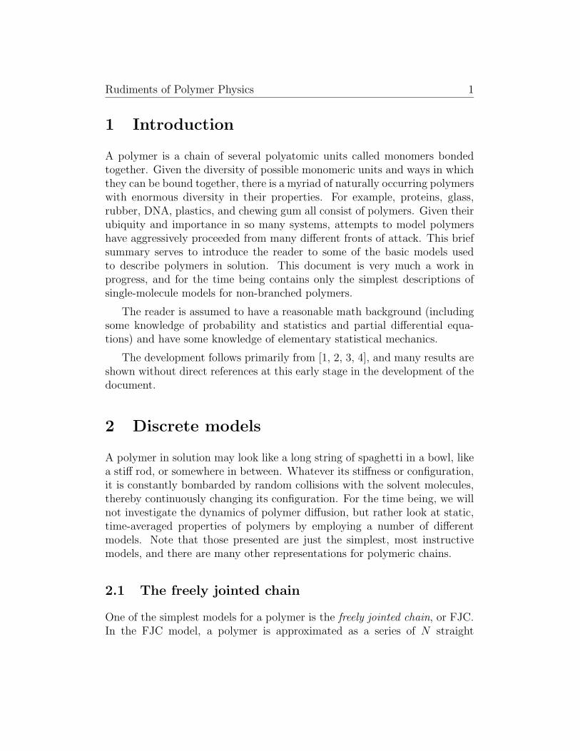
Figure 2.1: A drawing of a polymer and its representation as a FJC. Note that ri =

Ri −Ri−1 and that R = RN −R0 =N∑i=1

ri. The Ri’s are not important for the present

discussion, but become important as we move from discrete to continuous models in section3.

segments of a given length, b, as depicted in figure 2.1. The orientation ofeach segment of the FJC is independent of all others. The segment length, b,is called the Kuhn statistical length and describes the stiffness of the chain.If the Kuhn length is large, the chain tends to be stiff. Smaller Kuhn lengthsare characteristic of more flexible chains. ∗ In such a way, the parameter bdescribes the nature of short-range self-interactions of the polymer. In otherwords, if the orientation of a given small piece of the polymer is stronglycorrelated to the small piece immediately before it, b will be large, but ifthe orientation of the small piece of the polymer is unrelated to that of thepiece immediately before it, b will be small. So the Kuhn statistical lengthdescribes the minimum length between two points on a polymer that areessentially uncorrelated.

Since the orientation of each successive statistical segment vector (hence-forth referred to as simply “segment” for brevity), ri, is completely indepen-dent of all others, our model is without long-range self-interactions. This

∗It should be noted that, strictly speaking, this is not precisely a measure of the chainstiffness, since a Gaussian chain has no stiffness. The Kuhn statistical length is formallyonly a measure of chain stiffness for the Kratky-Porod wormlike chain. [5]


means that the chain can bend back and lay over itself. While this is physi-cally unrealistic, the FJC model is still extremely useful and often producesreasonable results in describing experimentally observed phenomena (e.g. in[6]).

Naturally, we would like the models we develop to provide all relevantthermodynamic information. Therefore, we would ultimately like to be ableto compute partition functions for polymer conformations. Rather than com-pute partition functions based on probability distributions for all possibleconformations, it is more convenient to use a probability distribution forthe end-to-end vector of the chain, R † , or the radius of gyration, Rg (theaverage distance of the polymer from its center of mass). These quantitiesmay be measured experimentally by light scattering experiments or by novelmore recently developed single molecule experiments (e.g. [6]). This is anal-ogous to using few-particle reduced distribution functions in other areas ofstatistical mechanics. [2] Therefore, we fill focus much of the discussion oncharacterizing the end-to-end vector, R, which is easier to handle than Rg.

Let Φ(R, N) be the probability distribution function for R given thatwe have a chain of N segments. Since the orientation of each segment isindependent of all others, Φ(R, N) will approach a Gaussian distribution forlarge N by the central limit theorem. Therefore, we need only to considerthe first and second moments to completely describe the distribution.

The first moment is easily calculated as

〈R〉 =

⟨N∑i=1

ri

⟩=

N∑i=1

〈ri〉 = 0 (2.1)

since 〈ri〉 = 0 ∀ i because the orientation of each vector is randomly dis-tributed. The second moment is also easily calculated:

R2 ≡ R ·R =

(N∑i=1

ri

)2

=N∑i=1

r2i + 2

N∑i=1

N−i∑j=1

ri · ri+j. (2.2)

⇒⟨R2⟩

=N∑i=1

⟨r2i

⟩+ 2

N∑i=1

N−i∑j=1

〈ri · ri+j〉 = N⟨r2i

⟩= Nb2 (2.3)

†Here, R is defined to be the end-to-end vector. In section 3, when we begin lookingat continuous models, R is a continuous representation of the vectors Ri in figure 2.1.


because 〈rn · rm〉 = 0 ∀ m 6= n since they are uncorrelated. Given the secondmoment, we arrive at the formal definition for the Kuhn statistical length:

b ≡ limL→∞

〈R2〉L

(2.4)

where L is the total path length of the chain, equal to Nb in this case. Takingthe limit in equation (2.4) is then trivial for the FJC. The second moment isoften used as a characteristic length of the chain. We have determined, then,that for a FJC,

R ≡√〈R2〉 = b

√N. (2.5)

Given both moments, Φ(R, N) is a Gaussian distribution with zero meanand a variance of

σ2 =⟨R2⟩− 〈R〉2 = Nb2. (2.6)

Thus,

Φ(R, N) =

(3

2πNb2

) 32

exp

(− 3R2

2Nb2

). (2.7)

Using Φ(R, N), we can obtain interesting insights on thermodynamicproperties. Following the development of [3], we assume that all conforma-tions with a given end-to-end distance are of equal energy. Then, we canobtain the entropy of the chain by equation (2.7) using the standard methodand absorbing all constants into the reference entropy.

S (R, N) ∝ k ln (Φ(R, N))

⇒ S = S0 −3kR2

2Nb2(2.8)

The free energy is then

F = E − TS = F0 +3kTR2

2Nb2(2.9)

We see that the free energy is related quadratically to the end-to-end vector,as if the chain is an “entropic spring”.

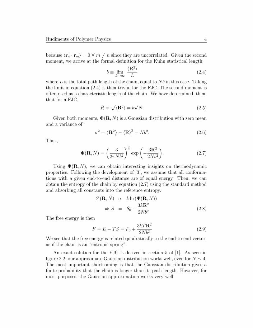
An exact solution for the FJC is derived in section 5 of [1]. As seen infigure 2.2, our approximate Gaussian distribution works well, even for N ∼ 4.The most important shortcoming is that the Gaussian distribution gives afinite probability that the chain is longer than its path length. However, formost purposes, the Gaussian approximation works very well.


0 1 2 3 4 5 6 7 8 9 100

0.2

0.4

0.6

(R2)1/2

4πR

2 Φ(R

)

Plot of 4πR2Φ(R) for b = 1

ApproximateExact

N = 25

N = 10

N = 7

N = 4

Figure 2.2: A plot of the exact and approximate solutions for a FJC. The approximationof large N appears to be reasonable even when N is below 10.


r3

r1

r2

rN

R

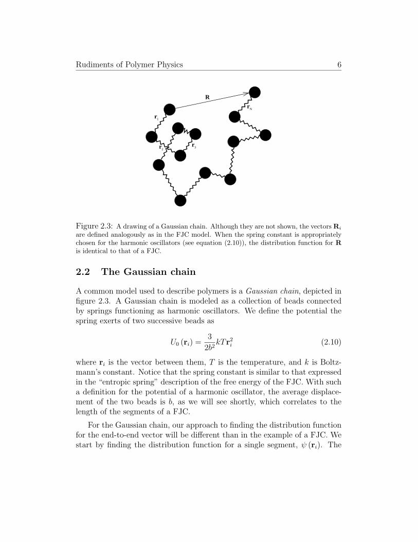
Figure 2.3: A drawing of a Gaussian chain. Although they are not shown, the vectors Ri

are defined analogously as in the FJC model. When the spring constant is appropriatelychosen for the harmonic oscillators (see equation (2.10)), the distribution function for Ris identical to that of a FJC.

2.2 The Gaussian chain

A common model used to describe polymers is a Gaussian chain, depicted infigure 2.3. A Gaussian chain is modeled as a collection of beads connectedby springs functioning as harmonic oscillators. We define the potential thespring exerts of two successive beads as

U0 (ri) =3

2b2kTr2

i (2.10)

where ri is the vector between them, T is the temperature, and k is Boltz-mann’s constant. Notice that the spring constant is similar to that expressedin the “entropic spring” description of the free energy of the FJC. With sucha definition for the potential of a harmonic oscillator, the average displace-ment of the two beads is b, as we will see shortly, which correlates to thelength of the segments of a FJC.

For the Gaussian chain, our approach to finding the distribution functionfor the end-to-end vector will be different than in the example of a FJC. Westart by finding the distribution function for a single segment, ψ (ri). The


probability will be Boltzmann weighted, so we have

ψ (ri) ∝ exp

(−U0

kT

)= exp

(−3r2

i

2b2

). (2.11)

Now we just have to normalize it, defining c as the normalization constantand ri ≡ |ri| and utilizing a Gaussian integral.∫

dri ψ (ri) = c

2π∫0

dφ

π∫0

dθ sin θ

∞∫0

dri r2i exp

(−3r2

i

2b2

)

= 4πc

∞∫0

dri r2i exp

(−3r2

i

2b2

)= c

(2πb2

3

) 32

= 1

⇒ c =

(3

2πb2

) 32

⇒ ψ (ri) =

(3

2πb2

) 32

exp

(−3r2

i

2b2

). (2.12)

This is a Gaussian distribution with 〈r2i 〉 = b2, thus verifying our claim of an

average bond length of b.

Since each segment is unrelated to the others, we can now write theconformational distribution function, Ψ ({ri} , L), which describes all possiblespacial orientations of the ri’s for a chain of total path length L.

Ψ ({ri} , L) =N∏i=1

ψ (ri) =

(3

2πb2

) 3N2

exp

(− 3

2b2

N∑i=1

r2i

). (2.13)

Now that we have the conformational distribution function, we can getthe end-to-end distribution function by

Φ (R, N) =

∫dr1

∫dr2 · · ·

∫drN δ

(R−

N∑i=1

ri

)Ψ ({ri} , L) , (2.14)

where the delta function serves to enforce that the end-to-end vector is givenby the sum of the segments. The calculation of the integral is lengthy and isomitted here, but the result is

Φ(R, N) =

(3

2πNb2

) 32

exp

(− 3R2

2Nb2

). (2.15)


The chain is thusly called a Gaussian chain because the bond lengths andthe end-to-end vector are Gaussian distributed. It should be noted that thismodel is by no means an adequate description of the local properties of thechain, but gives the same end-to-end vector distribution function as the FJC.For many applications, especially when the continuous analogs of the modelsare used, the Gaussian chain is the easiest to deal with mathematically andis therefore often used in place of the FJC (as we will do in section 3.1).

We note now that since each segment of the Gaussian chain is independentof the others, a chain of length N may be constructed by stringing twochains of length N1 and N2 together with N1 + N2 = N . Noting this, wecan trivially find the distribution function of the vector connecting any twoarbitrary segments m and n in a Gaussian chain.

Φ (Rn −Rm, n−m) =

(3

2πb2 |n−m|

) 32

exp

(−3 (Rn −Rm)2

2b2 |n−m|

). (2.16)

And similarly, ⟨(Rn −Rm)2⟩ = |n−m| b2. (2.17)

Now we will calculate the mean square radius of gyration, R2g, which is

the mean square distance between all the segments in the chain. Physically,this is the average distance of the chain from the center of mass,RG. Thus,


we can compute R2g following the development in [4].

RG =1

N

N∑m=1

Rm (2.18)

⇒ R2g =

1

N

N∑i=1

⟨(Ri −RG)2⟩

=1

N

N∑i=1

⟨(Ri −

1

N

N∑m=1

Rm

)2⟩

=1

N

N∑i=1

⟨R2i −

2Ri

N·

N∑m=1

Rm +1

N2

N∑m=1

N∑j=1

Rm ·Rj

⟩

=

⟨1

N

N∑i=1

R2i −

1

N2

N∑i=1

N∑m=1

Ri ·Rm

⟩

=1

2N2

N∑i=1

N∑m=1

⟨(Ri −Rm)2⟩ . (2.19)

Using equation (2.17), we can complete the calculation.

R2g =

1

2N2

N∑m=1

N∑n=1

|n−m| b2 ≈ b2

2N2

N∫0

dn

N∫0

dm |n−m|

=b2

N2

N∫0

dn

n∫0

dm (n−m) =N

6b2=〈R2〉

6. (2.20)

Approximating the sum as an integral gives a closed-form solution and isreasonable for large N . Figure 2.4 shows a comparison of the exact (given bythe sum) and the approximate closed-form mean square radius of gyration.

2.3 The freely rotating chain

Another reasonable model to describe chains absent of long-range self-interactionsis the freely rotating chain. A drawing of a freely rotating chain is shown infigure 2.5. The angle θ is fixed for each segment, but each segment can freely


100

101

102

100

101

102

N

Rg/b

2

Comparison of Discrete and Continuous Radii of Gyration

ContinuousDiscrete

Figure 2.4: A comparison of the approximate and exact mean square radii of gyrationfor a Gaussian chain. The approximation is reasonable even for N ∼ 10 and below.


R

r1

r2 r3

rN

ri−3

ri−2

ri−1

ri

θθ

θθ

Figure 2.5: At left, a 2-D representation of a freely rotating chain. As before, althoughthey are not shown, the vectors Ri are defined analogously as in the FJC model in figure2.1 and the lengths of each ri is again b. Note that full rotation is permissible about eachbond in the φ direction, as shown at right. Note also that each successive segment is notindependent of those previous to it. In such a way, the chain can exhibit stiffness for smallN .

rotate in the φ direction. The distribution function for the end-to-end vector,R, is difficult to obtain for the discrete case (we will examine a continuouslimit of this chain, called a Kratky-Porod wormlike chain, in a subsequentsection), so we will only compute R2 = 〈R2〉 here. This alone is enlighteningbecause it provides interesting insights into the limiting cases of this modeland the nature of the inherent stiffness.

Since equation (2.2) is general, it also holds for the freely rotating chain.A recursion relation is needed to calculate 〈ri · ri+j〉. The relationship isderived by successively projecting each segment vector, ri, onto the unitvector along the direction of the subsequent one, ri+1. Thus,

ri =(ri · ri+1) ri+1

|ri+1|2=

(ri · ri+1) (ri+1 · ri+2) · · · (ri+j−2 · ri+j−1)

(b2)j−1 ri+j−1.(2.21)

So, we have ri in terms of dot products of successive segments. We know fromelementary vector geometry that the dot product of the successive segmentsis

〈ri · ri−1〉 = b2 cos θ. (2.22)


The vector ri is then given by

ri =(b2)

j−1(cos θ)j−1

(b2)j−1 ri+j−1 = (cos θ)j−1 ri+j−1. (2.23)

Now we can calculate the relevant quantity:

〈ri · ri+j〉 = (cos θ)j−1 〈ri+j−1 · ri+j〉 = b2 (cos θ)j . (2.24)

Given that 〈r2i 〉 = b2, we have

⟨R2⟩

=N∑i=1

⟨r2i

⟩+ 2

N∑i=1

N−i∑j=1

〈ri · ri+j〉

= b2

(N + 2

N∑i=1

[N−i∑j=1

(cos θ)j])

. (2.25)

The sum in square brackets is itself a geometric series in cos θ with

N−i∑j=1

(cos θ)j =cos θ

(1− (cos θ)N−i

)1− cos θ

. (2.26)

Now we have

N∑i=1

N−i∑i=1

(cos θ)j =N∑i=1

cos θ(

1− (cos θ)N−i)

1− cos θ

=cos θ

1− cos θ

N∑i=1

1− (cos θ)N−i

=cos θ

1− cos θ

(N −

N∑i=1

(cos θ)N−i)

=cos θ

1− cos θ

(N − (cos θ)N

N∑i=1

(sec θ)i). (2.27)

The summation is a geometric series in sec θ. Using this fact and some


algebraic manipulations, we obtain

N∑i=1

N−i∑i=1

(cos θ)j =cos θ

1− cos θ

N − (cos θ)Nsec θ

(1− (sec θ)N

)1− sec θ

=

N cos θ

1− cos θ

(1− 1− (cos θ)N

N (1− cos θ)

). (2.28)

Substitution of equation (2.28) into (2.25) yields the final result of

⟨R2⟩

= Nb2

(1 +

2 cos θ

1− cos θ

(1− 1− (cos θ)N

N (1− cos θ)

))

= Nb2

(1 + cos θ

1− cos θ− 2 cos θ

N

1− (cos θ)N

(1− cos θ)2

). (2.29)

Clearly, if N is large, the second term vanishes and we get

R ≡√〈R2〉 = b

√N

(1 + cos θ

1− cos θ

), (2.30)

which shows that, as in the case of the FJC and Gaussian chains, the end-to-end distance scales as

√N . However if the second term is non-zero, the

chain is said to have “stiffness.”

To characterize how stiff the chain is, we wish to find some relationshipdescribing the “memory” of the chain. Suppose the first segment of the chainpoints in the direction u0. We now ask, how does the end-to-end vector ofthe chain, R, correlate with the original orientation, u0? If R is on averagealong the same direction as the original orientation, the chain is very stiff. Ifnot, it is more flexible. Thus, it is natural to calculate

〈R · u0〉 =

⟨R · r1

|r1|

⟩=

1

b

⟨r1 ·

N∑i=1

ri

⟩=

1

b

N∑i=1

〈r1 · ri〉 =1

b

N∑i=1

b2 (cos θ)i−1

= b

N∑i=1

(cos θ)i−1 = b1− (cos θ)N

1− cos θ. (2.31)

We used the results from equations (2.24) and (2.26) to arrive at this result.


100

101

102

103

104

0

5

10

15

20

25

30

35

40

45

50

ξp

<R

2 >1/

2

<R2>1/2 for b = 1 for various values of N

N = 50

N = 10

N = 30

N = 4

Figure 2.6: A plot of R ≡√〈R2〉 vs. ξp for a freely rotating chain. Note that R goes

to zero as ξp goes to zero. The appearance to the contrary in the plot is an artifact of thelogarithmic scaling.

In the limit of a long chain (large L = Nb),

limL→∞

〈R · u0〉 ≡1

2λ≡ ξp =

b

1− cos θ, (2.32)

where ξp is called the persistence length of the chain. This describes thestiffness in the chain in that it describes how long the orientation of thechain persists through its length. Clearly, the smaller θ is, the stiffer thechain will be. A θ of zero corresponds to a completely rigid rod. Figure 2.6shows how R ≡

√〈R2〉 varies with ξp for a freely rotating chain.

3 Continuous models

The models proposed thus far present a polymer chain as a set of discretesegments that have some relationship to each other. Based on the nature of


these relationships, we can construct a continuous model of the polymer thatdescribes the same characteristics as the discrete model.

3.1 The continuous Gaussian chain

In the discrete FJC, the segment length and the Kuhn statistical lengths wereone and the same. When we take a continuous limit, though, we naturallywant the limit as the segment length goes to zero. Therefore, we need to drawa distinction between the segment length and the Kuhn statistical length,which, as stated before, is a representation of the stiffness of the chain. ∗

Therefore, we define the segment length to be ∆s, where s denotes pathlength, and retain the same notation for the Kuhn statistical length, stillcalling it b. Thus, b2 becomes b∆s in our current development.

Next, we note that the total path length of a chain is L = N∆s. This, ofcourse, must be preserved as we take the continuous limit.

The necessary limits to take to get the continuous description are nowobvious. We take ∆s → 0, N → ∞, and N∆s → L. We define thislimit as the functional integral limit (limFI), since it defines a functionalintegral as a limit of the discrete chain. Since we will be integrating over theconformational distribution function, given by equation (2.13), we seek

limFI

d {ri} Ψ ({ri} , L) = limFI

d {Ri} Ψ ({Ri} , L)

= limFI

(N∏i=0

dRi

)Ψ ({Ri} , L) (3.1)

since the Ri’s are themselves simple functions of the ri’s.

For this analysis, we will follow the treatment of [2]. At first, we only

∗See footnote on page 2. The same comments apply to the persistence length. [5]


consider the exponential.

limFI

exp

(− 3

2b∆s

N∑i=1

r2i

)= lim

FIexp

(− 3

2b

N∑i=1

(Ri −Ri−1

∆s

)2

∆s

)

= limFI

exp

(− 3

2b

N∑i=1

(∂R

∂s

)2

∆s

)

= exp

− 3

2b

L∫0

ds

(∂R

∂s

)2. (3.2)

Here, R = R (s) is the continuous representation of the discrete case vectorsRi as a function of s and not the end-to-end vector of the chain. The lowerbound on the integral was obtained by defining the arbitrary reference pointfor R to be the starting point of the chain.

Now we will take limFI of the differential.

limFI

N∏i=0

dRi = DR. (3.3)

This denotes that the functional integral is defined as a limit of the iteratedintegrals for the discrete chain.

Finally, we’ll take the limit for the normalization constant.

limFI

(3

2πb∆s

) 3N2

= (∞)∞ . (3.4)

This appears to be a problem. However, the normalization is necessary toensure that the probability that the chain will be in some conformation isunity. Since it is just a normalization constant, it does not create any prob-lems when using the conformational distribution function. An easy way todeal with it is to define the normalization constant as N with the definitionδR ≡ N DR such that∫

R(0)=0

DR Ψ (R, L) =

∫R(0)=0

DRN exp

− 3

2b

L∫0

ds

(∂R

∂s

)2

≡∫

R(0)=0

δR exp

− 3

2b

L∫0

ds

(∂R

∂s

)2 = 1.(3.5)


Thus, we have arrived at a continuous conformational distribution func-tion for a Gaussian chain. We found

limFI

d ({ri}) Ψ ({r} , L) = DR Ψ (R, L) = δR exp

− 3

2b

L∫0

ds

(∂R

∂s

)2(3.6)

where R is a function of path length, s.

It should be noted that Ψ (R, L) may also be represented in terms of theunit tangent vector, u. We recall from differential geometry that

u =∂R

∂s. (3.7)

Taking Ψ as a function of u and finding Du from the dui’s in a mannersimilar to equation (3.3), we get

Du Ψ (u, L) = δu exp

− 3

2b

L∫0

dsu2

. (3.8)

3.2 The continuous freely rotating chain (Kratky-Porodwormlike chain)

To build a continuous analog to the freely rotating chain, we need to definea limit analogous to limFI for the Gaussian chain. Naturally, we want toretain similar limits as in limFI , so we put b→ 0, N →∞, and Nb→ L. Westill need to deal with θ. In the limit of b→ 0, the angle θ will go to zero, sowe impose θ → 0. Finally, we impose our definition of the persistence lengthgiven by equation (2.32). We will denote this limit limworm, since it is thelimit to get a Kratky-Porod wormlike chain.

Because we did not derive an expression for the conformational distribu-tion function for the freely rotating chain, we will only compute the contin-uous analogs for the end-to-end vector 〈R2〉 and for 〈R · u0〉.

In the calculation of 〈R2〉,Recall equation (2.29), repeated here for con-venience in reference:⟨

R2⟩

= Nb2

(1 + cos θ

1− cos θ− 2 cos θ

N

1− (cos θ)N

(1− cos θ)2

).


We first note that

(cos θ)N = exp (N ln (cos θ))

= exp

(N

(cos θ − 1− (cos θ − 1)2

2+ · · ·

))

= exp

(Nb

((cos θ − 1)

b− (cos θ − 1)2

2b+ · · ·

))(3.9)

since the Taylor expansion for the natural logarithm function is given by

lnx =∞∑k=1

(−1)k+1 (x− 1)k

k. (3.10)

To take limworm of this expression, we first apply equation (2.32), then putθ → 0, and finally put Nb→ L to get

limworm

(cos θ)N = exp (−2λL). (3.11)

With equation (3.11) in hand, we can evaluate the limit.

limworm

⟨R2⟩

= limworm

Nbb

1− cos θ(1 + cos θ)−

(b

1− cos θ

)2

cos θ(

1− (cos θ)N)

=L

λ− 1− exp (−2λL)

2λ2. (3.12)

Recalling equation (2.31) and (3.11), we can easily calculate the contin-uous analog for 〈R · u0〉 as

limworm

〈R · u0〉 = limworm

b

1− cos θ

(1− (cos θ)N

)=

1− exp (−2λL)

2λ. (3.13)

Using equations (3.12) and (3.13) and the definitions in of equations (2.4)and (2.32), we can calculate

b = limL→∞

〈R2〉L

=1

λ(3.14)

and

ξp = limL→∞

〈R · u0〉 =1

2λ. (3.15)


Therefore,

b = 2ξp, (3.16)

which is in general true. [5]

We can now look at important limiting cases. When the chain is muchlonger than its persistence length (λL � 1), the efects of the stiffness onthe end-to-end vector become negligible. Conversely, when the chain is shortcompared to its persistence length (λL � 1), the chain is very stiff. Wetake the appropriate limits recalling equations (3.12) and (3.13), employingl’Hopital’s rule when necessary.

limλL→∞

⟨R2⟩

= limλL→∞

L

λ− L2

2 (λL)2 (1− exp (−2λL)) =L

λ(3.17)

limλL→∞

〈R · u0〉 =1

2λ(3.18)

limλL→0

⟨R2⟩

= limλL→0

2λL− 1 + exp (−2λL)

2λ2

= limλL→0

2L2 (λL)− L2 + L2 exp (−2λL)

2 (λL)2

= limλL→0

2L2 − 2L2 exp (−2λL)

4λL

= limλL→0

4L2 exp (−2λL)

4= L2 (3.19)

limλL→0

〈R · u0〉 = limλL→0

L1− exp (−2λL)

2λL

= limλL→0

L2 exp (−2λL)

2= L (3.20)

Equations (3.17) and (3.18) give the random coil, (random flight) limitand equations (3.19) and (3.20) give the stiff rod limit.

We will return to the Kratky-Porod wormlike chain (WLC) in section3.4.2.


3.3 The Green function

In section 3.1 we found the conformational distribution function for a Gaus-sian chain, as given by equation (3.6). This signifies the probability distri-bution function for the polymer over all conformational space. Although wedid not explicitly find them, these distributions exist for other models. Thisdistribution provides more information than we need or want to (or can)deal with. Therefore, it is wise to find a reduced distribution function todescribe the system, since this is often all we need to extract thermodynamicinformation from experiments.[2] A good choice (and one we’ve been dealingwith in most of our developments) is to use the end-to-end vector distribu-tion function. We will define a conditional probability that fixes the end toend vector such that the chain begins at R′ and ends at R with total pathlength L. We call this the Green function (the rationale behind this namewill become clear later) and denote it as G (R,R′|L).

Given its definition, the Green function can be obtained by taking theappropriate integral over the conformational distribution function.

G (R,R′|L) =

R(L)=R∫R(0)=R′

δR Ψ (R, L) . (3.21)

Given the Green function, the conformational partition function for agiven end to end vector (R−R′) for a chain of total length L is given by

Z (R,R′|L) =

∫dR dR′G (R,R′|L) . (3.22)

In a manner similar to that on page 8, we can piece together two (andthree and four and . . .) chains. This is represented in the property of theGreen function given by

G (R,R′|L) =

∫dR′′G (R,R′′|L− l) G (R′′,R′|l) for l < L. (3.23)

An alternate (and equivalent) definition of the Green function is to defineits start at the origin, i.e. R′ = 0. Thus, its end-to-end vector is R−R′ = R.Then the Green function is denoted simply by G (R|L).


Often times other information pertaining to the conformation of the chainis important. The Green functions in equations (3.21) and (3.23) are validfor flexible chains. For chains with stiffness, the orientation, or unit tangentvector, u, of the chain is also important. In such a case, we can still defineG from the conformational distribution function. The trick is to incorporatethe end-to-end vector, R (assuming R′ = 0) into the integral. Given that uis the unit tangent vector for the chain,

R =

L∫0

dsu. (3.24)

Recalling equation (3.8), we can define the Green function for a chainwith length L, starting at the origin, ending at R, with initial orientationu0, and final orientation u as

G (R,u|u0, L) =

u(L)=u∫u(0)=u0

δu δ

R−L∫

0

dsu

Ψ (u, L) . (3.25)

3.3.1 The Green function for a Gaussian chain in an external field

Equation (3.6) gives the conformational distribution function for the Gaus-sian chain. If we were to place the chain in an external field (defined perunit length of the chain), Ue (R), the contribution of the field to the confor-mational distribution function is Boltzmann weighted. Thus, we get

Ψ (R, L) ∝ exp

− 3

2b

L∫0

ds

(∂R

∂s

)2

− 1

kT

L∫0

dsUe (R)

. (3.26)


For the case of the Gaussian chain represented by equation (3.26), we get

G (R,R′|L) =

R(L)=R∫R(0)=R′

δR Ψ (R, L)

=

R(L)=R∫R(0)=R′

δR exp

− 3

2b

L∫0

ds

(∂R

∂s

)2

− 1

kT

L∫0

dsUe (R)

(3.27)

= limFI

∫dR0 δ (R0 −R′)

∫ ( N∏i=1

dRi

)N δ (RN −R)

× exp

(− 3

2b∆s

N∑i=1

(Ri −Ri−1)2 − ∆s

kT

N∑i=1

Ue

(Ri −Ri−1

2

))(3.28)

Note that the Green function is defined as a functional integral, a limit of aniterated integral. [2]

3.3.2 The Green function for a WLC in an external field

We did not directly arrive at a Ψ (R) for the Kratky-Porod wormlike chain.We will use the result proven in [1, 5] and assert that the WLC may betreated as a differential space curve. We know from elasticity theory thatthe bending energy for a stiff rod of length L is given by

U =ε

2

L∫0

ds

(∂u

∂s

)2

, (3.29)

where ε is the bending modulus. For a WLC, this bending modulus is givenby

ε =kT

2λ. (3.30)

The conformational distribution function is just a Boltzmann weighting ofthis bending energy.

Ψ (u, L) ∝ exp

− 1

4λ

L∫0

ds

(∂u

∂s

)2. (3.31)


Adding in the Boltzmann weighted energy from the external field, we get

Ψ (u, L) ∝ exp

− 1

4λ

L∫0

ds

(∂u

∂s

)2

− 1

kT

L∫0

dsUe (R)

. (3.32)

Thus, the Green function is given by taking the appropriate integral overthe conformational distribution function per equation (3.25). We must takethe functional integral limit as in equation (3.27), but we will not show thatexplicitly.

G (R,u|u0, L) =

u(L)=u∫u(0)=u0

δR δ

R−L∫

0

dsu

× exp

− 1

4λ

L∫0

ds

(∂u

∂s

)2

− 1

kT

L∫0

dsUe (R)

. (3.33)

3.4 The Green function as a solution to a partial dif-ferential equation

As we saw in the discussions at the beginning of section 3.3, obtaining theGreen function for a polymer configuration reveals all of the thermodynamicinformation for the chain. However, the forms of the Green functions givenby equations (3.27) and (3.33) are entirely cumbersome and difficult to usein any practical sense. Therefore, it would be very beneficial to find analternate, more tractable representation of the Green function.

It turns out that by employing the techniques of Feynman and Hibbs [7],we can derive partial differential equations that describe the Green function.We will derive the PDE for the continuous Gaussian chain following thedevelopment of [2] and state the result for the WLC as derived by [5].

3.4.1 The Gaussian chain governing PDE

Assume we have a chain with Green function G (R,R′|L). Now we increasethe chain length from L to L+ ε where ε is small. Using equation (3.27), we


can write

G (R,R′|L) =R(L+ε)=R∫R(0)=R′

δR exp

− 3

2b

L+ε∫0

ds

(∂R

∂s

)2

− 1

kT

L+ε∫0

dsUe (R)

(3.34)

Using equation (3.23), we can write

G (R,R′|L+ ε) =

∫dR′′G (R,R′′|ε) G (R′′,R′|L) . (3.35)

Here, we have specified that R′′ ends at the point on the chain correspondingto path length L. In doing this, there is a tiny piece of the chain betweenL and L + ε, i.e. between R′′ and R. The Green’s function between thesetwo points will approach a delta function as ε → 0. We can employ thedefinition of the delta function which describes it as a limit of the Gaussiandistribution. Thus, for small ε,

G (R,R′′|ε) ≈(

3

2πbε

) 32

exp

(−3 (R−R′′)2

2bε− ε

kTUe

(R + R′′

2

)).(3.36)

The term with Ue is negligible in the limit of small ε, so this is still a validrepresentation of the delta function.

Substituting equation (3.36) into (3.35) gives

G (R,R′|L+ ε) =

(3

2πbε

) 32∫dR′′ exp

(−3 (R−R′′)2

2bε− ε

kTUe

(R + R′′

2

))×G (R′′,R′|L). (3.37)

We make the substitution of R′′ = R + η with dR′′ = dη. This gives

G (R,R′|L+ ε) =(3

2πbε

) 32∫dη exp

(−3η2

2bε− ε

kTUe

(R +

η

2

))G (R + η,R′|L) . (3.38)

It is now convenient to Taylor expand the respective terms in equation(3.38). We notice that

limε→0+

(3

2πbε

) 32

exp

(−3η2

2bε

)= δ (η) . (3.39)


The term has an essential singularity as ε→ 0+ because it is a delta functionin that limit. Furthermore, for small ε, the delta function ensures that onlyterms with very small η contribute significantly to the integral. Thereforewe should Taylor expand the rest of the terms about η = 0.

1

kTεUe

(R +

η

2

)=

1

kT

(εUe (R) +

ε

2η · ∂Ue

∂R

)+O (εη) . (3.40)

We substitute this expansion into the exponential and then expand the ex-ponential to get

exp

(−εUekT

(R +

η

2

))= 1− 1

kTεUe (R) +O (εη) (3.41)

Now we Taylor expand the two Green functions

G (R,R′|L+ ε) = G (R,R′|L) + ε∂

∂LG (R,R′|L) +O

(ε2)

(3.42)

and

G (R + η,R′|L) = G (R,R′|L) + η · ∂∂R

G (R,R′|L)

+1

2ηη :

∂2

∂R2G (R,R′|L) +O

(η3, η4

). (3.43)

Here, : denotes the dyadic product. Since after expansion all Green functionsare of the same form, we will define G ≡ G (R,R′|L) for brevity. We cannow put it all together to get

G + ε∂G

∂L+O

(ε2)

=

(3

2πbε

) 32∫dη exp

(−3η2

2bε

)(1− 1

kTεUe (R) +O (εη)

)×(

G + η · ∂∂R

G +1

2ηη :

∂2

∂R2G +O

(η3, η4

))(3.44)

Before we multiply the sums together, we should note that G is not a functionof η. We note further that all the integrals with respect to η are Gaussianintegrals of the form(

3

2πbε

) 32∫dη ηn exp

(−3η2

2bε

), n integer, (3.45)


which is a standard Gaussian integral. These integrals are zero for all oddpowers of n. The integrals for n = 0, 2, 4 are(

3

2πbε

) 32∫dη exp

(−3η2

2bε

)= 1 (3.46)(

3

2πbε

) 32∫dη η2 exp

(−3η2

2bε

)=

bε

3(3.47)(

3

2πbε

) 32∫dη η4 exp

(−3η2

2bε

)= ε2. (3.48)

Taking all odd powered Gaussian integrals to be zero, substituting equa-tions (3.46), (3.47), and (3.48) into equation (3.44), and simplifying yields

ε

(∂

∂L− b

6

∂2

∂R2+UekT

)G +O

(ε2)

= 0. (3.49)

Diving by ε and taking ε→ 0 yields(∂

∂L− b

6

∂2

∂R2+UekT

)G = 0. (3.50)

We must now define the boundary conditions. Harking back to equation(3.36), we put ourselves at the start of the chain. For a very short chain,G (R,R′|ε) approaches a delta function as ε→ 0+. Thus, our first boundarycondition is

G (R,R′|0) = δ (R−R′) . (3.51)

Next, we note that L < 0 is nonsense and G has a discontinuity across zero.Thus, we have arrived at our final partial differential equation to describe aGaussian chain in an external field.(

∂

∂L− b

6

∂2

∂R2+UekT

)G (R,R′|L) = δ (R−R′) δ (L) (3.52)

The equation is a diffusion-like equation with L being the “time” and b6

being the diffusivity. The external field makes the solution difficult, which iswhy excluded volume is so difficult to deal with.


3.4.2 The wormlike chain governing PDE

The governing PDE for the wormlike chain is derived using a similar tech-nique. The result, taken from [5], is stated here without proof. This solutionsets R′ ≡ 0.(

∂

∂L− λ ∂2

∂u2+ u · ∂

∂R+UekT

)G (R,u|u0, L) =

δ (u− u0) δ (R) δ (L) (3.53)

In this equation, we see that the “orientation” is diffusing with a diffu-sivity proportional to the inverse of the persistence length. Thus, the morestiff the chain is, the more slowly the orientation will diffuse along the chainand the longer a given orientation will persist. Aside from the “time” term(represented by the differential with respect to L), there is also a convectionterm for the position of the chain.

4 Conclusions

We have seen three discrete and two continuous models used to describepolymers. Even though they are simple in concept, they become complicatedquickly while manipulating them. The K-P WLC in an external field isoften only solvable numerically. Furthermore, it the stiffness parameter hasany nontrivial functionality, the PDE of equation (3.53) has nonconstantcoefficients. While using these and other models, one should choose thesimplest model possible to achieve the results he desires.

These models are the cornerstone of many studies in polymer physicsand will be the starting point as we delve into studies in excluded volume,self-interactions, concentrated polymer solutions, and polymer dynamics.

References

[1] Hiromi Yamakawa. Modern Theory of Polymer Solutions. Harper Row,electronic edition, 1971. Available at http://www.molsci.polym.kyoto-u.ac.jp/archives/redbook.pdf.


[2] Karl F. Freed. Functional integrals and polymer statistics. Advances inChemical Physics, 22:1–128, 1972.

[3] Pierre-Gilles de Gennes. Scaling Concepts in Polymer Physics. CornellUniversity Press, 1979.

[4] Masao Doi and Sam F. Edwards. The Theory of Polymer Dynamics.Oxford University Press, 1986.

[5] Hiromi Yamakawa. Helical Wormlike Chains in Polymer Solutions.Springer-Verlag, 1997.

[6] Steven B. Smith, Yujia Cui, and Carlos Bustamante. OverstretchingB–DNA: The elastic response of individual double–stranded and single–stranded DNA molecules. Science, 271:795–799, 9 February 1996.

[7] Richard P. Feyman and Albert R. Hibbs. Quantum Mechanics and Inte-grals. McGraw-Hill, 1965.

rudiments of polymer physics

Documents