Thermodynamics and its applications – an overview

by

R.T. Jones

E-mail: rtjones@global.co.za

Abstract: The laws of thermodynamics provide an elegant mathematical expression of some empirically-discovered facts of nature. The principle of energy conservation allows the energy requirements for processes to be calculated. The principle of increasing entropy (and the resulting free-energy minimization) allows predictions to be made of the extent to which those processes may proceed.

Originally presented at: SAIMM Pyrometallurgy School

Mintek, Randburg, 20-21 May 1997

1

1 INTRODUCTION Pyrometallurgy, by its very nature, involves high temperatures and the application of energy to materials. For this reason, the study of thermodynamics is one of the most important fundamentals of the subject. 1.1 What is thermodynamics? Thermodynamics is a collection of useful mathematical relations between quantities, every one of which is independently measurable. Although thermodynamics tells us nothing whatsoever of the microscopic explanation of macroscopic changes, it is useful because it can be used to quantify many unknowns. Thermodynamics is useful precisely because some quantities are easier to measure than others. The laws of thermodynamics provide an elegant mathematical expression of some empirically-discovered facts of nature. The principle of energy conservation allows the energy requirements for processes to be calculated. The principle of increasing entropy (and the resulting free-energy minimization) allows predictions to be made of the extent to which those processes may proceed. Thermodynamics deals with some very abstract quantities, and makes deductions using mathematical relations. In this, it is a little like mathematics itself, which, according to Bertrand Russell, is a domain where you never know a) what you’re talking about, nor b) whether what you’re saying is true. However, thermodynamics is trusted as a reliable source of information about the real world, precisely because it has delivered the goods in the past. Its ultimate justification is that it works. Confusion in thermodynamics can easily result if terms are not properly defined. There is no room for the loose use of words in this subject. 1.2 Energy or Heat Many books on thermodynamics contain vague and strange statements, such as ‘heat flows’, or ‘heat is a form of energy’, or ‘heat is energy in transit’, or it is ‘energy at a boundary’, or it is ‘the process’, or ‘the mechanism by which energy is transferred’. Work is ‘being done’ or is ‘being transformed into heat’. Heat and work, these ‘two illegitimate troublemakers’, in the words of Barrow1, do not provide a proper base on which to build thermodynamics. Heat and work seem to float between the system we deal with and its surroundings. They are not properties of the system we are dealing with, or of any other system. The quantities q and w (to be defined later) should not be mixed with actual properties like energy and heat capacity. In contrast to heat and work, energy is a well-defined property. It has its origin in the ideas of the potential and kinetic energy of simple mechanical systems. Experiments such as Joule’s ‘mechanical equivalent of heat’ let us extend the concept, and definition, to include thermal energy. Then, using the idea of the conservation of energy, changes in the energy of a chemical system of any complexity can be dealt with.

2

A niche can, however, be found for the action terms ‘heating’ and ‘doing work’. They can be used to indicate that the process by which the energy of the system changes is accompanied by a change in the thermal or the mechanical surroundings. According to Barrow1, our attachment to ‘heat’ stems from the caloric theory of the 18th and 19th centuries. That theory held that heat was a manifestation of a material called ‘caloric’. This material flowed in and out of objects when the temperature changed. Studies such as those of Mayer, Thompson, and Joule showed that caloric could be created or destroyed and, therefore, that heat was not one of the substances of the material world. The ‘caloric period’ had come to an end. By continuing to use ‘heat’, we remain tied to the myths of the past. It is time to give up this awkward remnant and to continue building thermodynamics on the sound foundation of ‘energy’ alone.

2 STATE FUNCTIONS (THE BUILDING BLOCKS) State functions are quantities whose values depend only on their current state, not on how they got to that state. Height above mean sea level is an example of this. It is not necessary to know anything about the path followed to a particular point, as long as one can measure the altitude at the destination. Obviously, the distance covered or the work expended on the journey depend very much on the route chosen and the mode of transport. For the calculation of state functions, it is possible to use an imaginary route to get to the destination, without changing the final answer. While processes are physical, and occur generally as a series of non-equilibrium stages, paths (used for purposes of convenient calculation) are mathematical abstractions. Fortunately, enthalpy (H), entropy (S), and Gibbs free energy (G) are all state functions. All good introductions to thermodynamics show the functional dependence of enthalpy, entropy, and Gibbs free energy (of a particular substance) on variables such as temperature and pressure. These thermodynamic functions may be expressed in terms of other variables, such as volume, for example, using straightforward mathematical transformations. However, the state variables that are of primary interest to pyrometallurgists are temperature and pressure.

H = H (T, P) [1]

S = S (T, P) [2]

G = G (T, P) [3] It is accepted for now that the functions H, S, and G are clearly defined, and that known values for these functions exist or can be measured. An equation of state (such as PV = nRT for an ideal gas) is used to calculate the interrelation between the measurable properties P, V, and T. Most processes of interest to pyrometallurgists can be idealized as operating at constant temperature (isothermal) or constant pressure (isobaric). The requirement of constant volume (isochore, or isometric) is less commonplace.

3

As will be shown in the next section, the energy required for any steady-state flow process is essentially the difference in enthalpy between the products and reactants, plus the amount of energy lost to the surroundings. The change in enthalpy over the process is easily calculated if the enthalpies of all the chemical species are calculated relative to the same reference state, namely that of the elements in their standard states at 25°C and 1 atm. By choosing the elemental reference state, the difference in enthalpy can be calculated without having to take into account any of the chemical reactions which may have taken place. (If there are no reactions, it is alright to use compounds as the basis, but the basis specified above is easy to remember and is always applicable. This is, therefore, strongly recommended.) Because the thermodynamic functions of interest, namely enthalpy, entropy, and Gibbs free energy, are all state functions, their values can be calculated independently of any reaction path. In general, the partial molal enthalpy of any chemical species is a function of temperature, pressure, and composition. The effect of composition on the enthalpies of individual components is small in most cases, and, in any case, there is very little data available on the variation in enthalpy with composition. The effects of composition on enthalpy are therefore usually ignored, which is equivalent to the treatment of the process streams (at least for this purpose) as ideal solutions (i.e. the enthalpy of mixing is taken to be zero). Except for gases under high pressure, the dependence of enthalpy on pressure is small. (If deemed important, the effect could be allowed for by the use of equations of state, or reduced property correlations.) In the field of high-temperature chemistry, the enthalpy is often assumed to depend solely on temperature. The total enthalpy of a stream is taken to be equal to the sum of the enthalpies of all the chemical species in the stream. For each chemical species*:

∫∫ +++∆=T

TP

T

TPof dTCLdTCHH

12

1

29811298 [4]

∫∫ +++=T

T

PT

TPo dTT

CT

LdT

TC

SS1

21

298

11298 [5]

where:

H = enthalpy of chemical species relative to elements in their standard states at 25°C and 1 atm (J / mol)

ofH 298∆ = standard enthalpy of formation of the species at 298K (J/mol)

T1 = phase transition temperature (K) CP(T) = a + bT + cT-2 + dT2 (J/mol/K) (subscripts 1 and 2 refer to different phases) T = temperature (K) LT1 = latent energy of phase transformation (J/mol) S = absolute entropy of chemical species relative to elements in their

standard states at 25°C and 1 atm (J/mol/K) oS 298 = standard entropy of the species at 298K (J/mol/K)

* Note: The singular of species remains species, not specie which means ‘coins’.

4

Also: G = H - T S [6]

where

G = Gibbs free energy of chemical species relative to elements in their standard states at 25°C and 1 atm (J/mol)

Note that equations [4] and [5] may easily be extended to cover the situation where more than one phase transition occurs. For computational convenience, the enthalpy and entropy can be evaluated by performing a single integration in each case. In order to do this, the first terms of equations [4] for enthalpy and [5] for entropy can be combined as integration constants. In this way, the same equations can be used, with different sets of constants being applicable to each temperature range. The upper temperature of each range is often the temperature of a phase transformation at a pressure of one atmosphere, but this need not necessarily be the case. For example, the data on gases come to an end at a temperature that is determined by the range of the experimental measurements. Also, in cases where it is difficult to adequately represent the CP term with a four-term expression (for example), the temperature range for a particular phase can be arbitrarily divided, in order to obtain a more accurate fit to the data. The following equations now apply:

∫+∆=T

Pof dTCHH

298298 "" [7]

∫+=T

Po dTT

CSS

298298 "" [8]

CP(T) = a + bT + cT-2 + dT2 [9]

Equations [7], [8], and [9] apply to a particular phase (or temperature range), and the constants a, b, c, and d are specific to that range. Note that “ o

fH 298∆ ” and “ oS 298 ” may be considered to be the standard enthalpy of formation and standard entropy of the phase in its metastable state at 298K. To calculate the enthalpy and entropy of a particular compound at a given temperature, it is necessary to obtain the correct values of the constants that pertain to that particular temperature range. By default, the program selects the thermodynamic constants of the most stable phase of each species at the specified temperature. To explain further, o

fH 298∆ refers to the standard isothermal enthalpy change for the formation reaction from the most stable phases of the elements at 25°C and 1 standard atmosphere pressure. oS 298 is the absolute (or Third Law) entropy of the phase at 25°C and 1 atmosphere. In cases where there is more than one data set for a given phase, “ o

fH 298∆ ”

and “ oS 298 ” refer to the properties that would be reported at 25°C and 1 atmosphere if the CP function behaved near this standard condition the way it does in the specified temperature range. As we are dealing merely with convenient integration constants, it should not be surprising that the ‘absolute entropy’ for some unstable phases at 25°C may be negative. The

5

fictitious entropy constants are useful only for purposes of facilitating the computation of the actual entropy at higher temperatures where the phase in question is stable. As thermodynamic data are not too readily available for minerals as such, it is often necessary to treat these as mixtures of chemical species. This is fairly straightforward for most minerals.

3 PRINCIPLE OF ENERGY CONSERVATION (FIRST LAW) The conservation equations for matter in general can sometimes be rather complicated. Fortunately, these can usually be simplified. The First Law of thermodynamics is not a general energy balance, but represents the balance of internal energy for a material with very particular constitutive properties, in particular, the absence of irreversible energy transfer. In essence, the First Law of thermodynamics states that the energy of an isolated system (one that does not exchange matter or energy with its surroundings) remains constant. For non-nuclear processes, the principle of energy conservation states that the sum of the changes of the extensive properties kinetic energy (Ek), potential energy (Ep), and internal energy (U) is equal to the sum of the modes of energy transfer q (defined as the thermal transfer of energy) and w (defined as the mechanical transfer of energy).

∆Ek + ∆Ep + ∆U = q + w [10] This equation is applicable to all constant-matter systems in general, and to steady flow processes in particular. By assuming mechanical equilibrium for the entering and exiting regions of a hypothetical volume, it is possible to produce a general equation relating the change in enthalpy to the sum of the thermal transfer of energy and the so-called shaft work, ws, and the change in the product of the pressure, P, and volume, V, as shown in equation [11]. One of the fundamental relations of thermodynamics is used in equation [12] to relate the change in enthalpy, H, to the change in internal energy, U.

w = ws + ∆PV [11]

∆H = ∆U + ∆PV [12] Therefore

∆Ek + ∆Ep + ∆H = q + ws [13] However, for most chemical systems of interest, the changes in kinetic and potential energy are very small compared to the changes in ∆H. This allows us to simplify equation [13] as follows.

∆H = q + ws [14] This equation allows us to calculate the amount of energy transferred to or from any process, simply by calculating the difference in enthalpy before and after. As enthalpy, H, is a state

6

function, its value does not in any way depend on the process itself or on the imaginary path followed during the process. Enthalpy is a function of temperature and pressure only. However, the dependence on pressure is small in most cases, and is usually ignored at reasonable pressures. A process is said to be endothermic when ∆H > 0, and exothermic when ∆H < 0. 3.1 Thermo software Chemical thermodynamics is a clear, simple, and elegant subject, if one does not get bogged down by the details. Fortunately, readily available computer software is able to provide the tools for performing thermodynamic calculations. Such software, containing suitable data, is able to calculate the standard enthalpy, entropy, and Gibbs free energy of different chemical species at any specified temperature. Unit conversions, such as from J/mol to kWh/kg, are also able to be performed automatically. The software is able to check the consistency of stoichiometry of reactions, such as Cr2O3 + 3C = 2Cr + 3CO, and to calculate the standard thermodynamic functions for the reaction, with specified reactant and product temperatures. The thermodynamic functions can be tabulated and depicted graphically. 3.2 Energy balances using the Thermo program Note well that it is correct to talk about an energy balance, but incorrect to talk of a heat balance (as ‘heat’ does not exist anyway) or an enthalpy balance (as enthalpy is conserved only in very special cases). The First Law of thermodynamics deals with the conservation of energy, and energy alone! Note also, in the examples that follow, the effects of pressure on enthalpy, and the physical effects of mixing are neglected (justifiably, as they are small relative to the other quantities). 3.3 Example 1 – Melting of iron Consider a small furnace containing 100 kg of iron at room temperature (nominally 25°C) that needs to be melted and heated to a temperature of 1600°C. (It can be assumed that the losses of energy through the walls and roof of the furnace can be ignored for our purposes.) If the furnace is set to supply 160 kW, the time taken for this process can easily be calculated. Iron undergoes a number of solid-state phase changes on being heated, and then melts around 1536°C. However, this poses no complication for the calculation of the energy balance, as the enthalpy of the iron is a state function (and is therefore independent of the path followed). Figure 1 shows the standard enthalpy of formation of Fe as a function of temperature. (Remember that the enthalpy is a function of pressure also, but the dependence is small.) In most compilations of enthalpy tables, pressure is not mentioned, as the small effect can be safely ignored at reasonable pressures.

7

Figure 1: The standard enthalpy of formation of Fe, as a function of temperature

Relative to the standard state of iron at 25°C and 1 atm having an enthalpy of zero, the enthalpies are readily obtained. As can be seen in Figure 2, the standard enthalpy of formation of Fe is 0.00 kJ/mol at 25°C, and 75.90 kJ/mol at 1600°C. The difference of 75.90 J/mol or 0.377 kWh/kg is easily obtained by subtraction. In our case, we would use this information to say that 100 kg of iron requires 100 x 0.377 kWh. At a power rating of 160 kW, this would take (37.7 / 160) hours or 14 minutes.

Figure 2: The heating of Fe from 25° to 1600°C

8

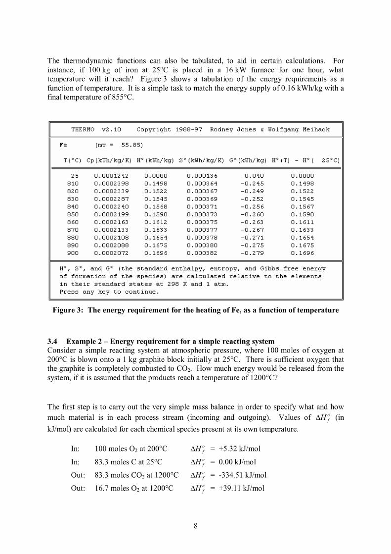
The thermodynamic functions can also be tabulated, to aid in certain calculations. For instance, if 100 kg of iron at 25°C is placed in a 16 kW furnace for one hour, what temperature will it reach? Figure 3 shows a tabulation of the energy requirements as a function of temperature. It is a simple task to match the energy supply of 0.16 kWh/kg with a final temperature of 855°C.

Figure 3: The energy requirement for the heating of Fe, as a function of temperature

3.4 Example 2 – Energy requirement for a simple reacting system Consider a simple reacting system at atmospheric pressure, where 100 moles of oxygen at 200°C is blown onto a 1 kg graphite block initially at 25°C. There is sufficient oxygen that the graphite is completely combusted to CO2. How much energy would be released from the system, if it is assumed that the products reach a temperature of 1200°C?

The first step is to carry out the very simple mass balance in order to specify what and how much material is in each process stream (incoming and outgoing). Values of o

fH∆ (in kJ/mol) are calculated for each chemical species present at its own temperature.

In: 100 moles O2 at 200°C ofH∆ = +5.32 kJ/mol

In: 83.3 moles C at 25°C ofH∆ = 0.00 kJ/mol

Out: 83.3 moles CO2 at 1200°C ofH∆ = -334.51 kJ/mol

Out: 16.7 moles O2 at 1200°C ofH∆ = +39.11 kJ/mol

9

It is now a simple matter to calculate the total enthalpy entering and leaving the system. The energy requirement for this process is therefore [(83.3 x –334.51) + (16.7 x 39.11) – (100 x 5.317) - (83.3 x 0.00)] = -27 744 kJ. Note that we have not needed to use the value of o

rH∆ at 1200°C (-396.2 kJ/mol) in our calculations, as the energy balance is concerned only with the initial and final states of the system, and not with any reactions that might have taken place along the way. Figure 4 illustrates how this calculation may be performed directly, using the Thermo computer program.

Figure 4: Energy balance calculation for a simple reacting system

3.5 Complex balances A simple procedure suffices for the calculation of energy balances in even the most complex systems. By a sensible choice of a reference state, energy balance calculations can be carried out without reference to the process or reaction paths.

a. Calculate a mass balance for the system in terms of molar quantities of each species entering an leaving the system.

b. Use the Thermo (or other) program to calculate the value of ofH∆ (in J/mol) for each

chemical species present at the entering and leaving temperature. The recommended reference state is one where the elements in their standard state at 25°C and 1 atm have a standard enthalpy of formation of zero.

c. Calculate the total enthalpy of each process stream entering and leaving the system. This is done by multiplying the number of moles of each species in the stream by the value

10

obtained for ofH∆ for the species at the temperature of the stream. (If deemed important,

the effects of pressure and mixing can be included at this point.) d. The energy requirement of the process is equal to the difference in enthalpy between the

products and reactants, plus the amount of energy lost to the surroundings. 3.6 Example 3 – Roasting of zinc sulphide The roasting of zinc sulphide is an example of an autogenous process, i.e. one which is able to supply enough energy to sustain the reaction without requiring an additional energy source. In the course of practical operation of the process, it is necessary to know how much of a surplus or deficit of energy there is, under a specified set of conditions, so that the appropriate control actions may be taken. Suppose the roasting of zinc sulphide can be simplified as follows. ZnS at 25°C is fed to a fluidized-bed reactor, together with pre-heated air at 200°C. We will assume for now that all the ZnS is converted to ZnO, and that all the sulphur is converted to SO2, as per the reaction:

ZnS + 3/2 O2 = ZnO + SO2 It is desired to have the products leaving the reactor at 900°C. Air is fed in excess, say 1.5 times the amount of oxygen required by the reaction. Obviously, this introduces N2 into the system in the proportion normally present in air (i.e. 8.46 moles of N2 to 2.25 moles of O2). The nitrogen does not take part in the reaction, but affects the energy requirement of the process, as it enters the process at 200°C and leaves at 900°C.

Figure 5: Roasting of zinc sulphide

The result of the calculation, shown in Figure 5, shows that the system needs to be cooled by 0.448 kWh/kg of ZnS. In practice, the reactor loses energy to the surroundings by

11

convection, radiation, and conduction from the walls of the reactor. Additional cooling may be achieved by using a water spray on the walls (or even adding water with the charge to the reactor). Alternatively, more air could be added, or the degree of preheating could be reduced. 3.7 Example 4 – Adiabatic flame temperature Adiabatic conditions are those in which there is no thermal transfer of energy between a system and its surroundings. In the combustion of fuels, the adiabatic flame temperature sets an upper limit on the temperature that may be achieved in a system. The adiabatic flame temperature is the temperature attained in a reacting system that experiences no loss of energy. The adiabatic flame temperature may be calculated by finding the temperature at which the total enthalpy of the products (at the product temperature) is the same as that of the reactants (at their initial temperatures). In the case of propane being fully combusted by air (initially at ambient temperature), the reaction may be written as shown in Figure 6. The adiabatic flame temperature is found (by trial-and-error variation of the temperature until the enthalpy difference is approximately zero) to be 2121°C in this case.

Figure 6: Calculation of adiabatic flame temperature (where ∆H ≈ 0)

4 PRINCIPLE OF INCREASING ENTROPY (SECOND LAW) C.P. Snow2 once suggested the second law of thermodynamics as a test of scientific literacy for the humanist, and said it was ‘about the scientific equivalent of: Have you read a work of Shakespeare’s?’. Yet, most people in the scientific world also have many misconceptions about the concept of entropy.

12

It is tempting, but rather a waste of time, to inquire into the ‘meanings’ of thermodynamic functions such as enthalpy or entropy. Thermodynamics reveals nothing of any microscopic or molecular meaning for its functions. It is widely assumed that entropy measures the degree of disorder, randomness, or ‘mixed-upness’ of a system. In fact, the entropy change which occurs when an isolated body moves spontaneously toward equilibrium is, according to thermodynamics, always positive. By the methods of statistical mechanics, the entropy increase in such an isolated body can be simply related to the increase in the number of independent eigenstates to which the isolated body has access. This number can be simply related to the purely geometrical or spatial mixed-upness in only three very special cases, namely mixtures of perfect gases, mixtures of isotopes, or crystals at temperatures near absolute zero, none of which is commonly studied in the ordinary chemical laboratory, let alone in high-temperature furnaces. In all other cases, the entropy change is capable of no simple quasi-geometrical interpretation, even for changes in isolated bodies. But the situation is even worse than this, for chemists commonly behave not only as if entropy increases in isolated bodies were a measure of disorder, but also as if this were true of entropy changes at constant temperature and pressure, under which conditions, very different from isolation, most chemical reactions are actually carried out. Even if the entropy change were a measure of disorder in an isolated body, the corresponding measure in an isothermal and isobaric experiment would be the Gibbs free-energy function and not the entropy. Misunderstandings regarding entropy have led to some widely-held misconceptions, such as the so-called ‘heat-death’ of the universe. McGlashan3 rather eloquently refutes this idea by pointing out some of the misconceptions on which it is built. The argument runs something like this. Any process which actually takes place in the universe increases the entropy of the universe. Increase of entropy implies an increase in disorder. Therefore, the ultimate fate of the universe is chaos. If thermodynamics could be shown (but how?) to be applicable to the universe, and if the universe were known to be a bounded and isolated body, then we might deduce that the universe would eventually reach a state of complete equilibrium. But there is no scientific reason to suppose that the universe is a bounded isolated body. Even if it were, there is no reason to suppose that the experimental science of thermodynamics can be applied to bodies as large as the universe. The principle of increasing entropy (and the resulting free-energy minimization) allows predictions to be made as to the extent to which those processes may proceed. The concept of entropy is of limited direct use for open systems, and the concept of free energy (G = H – TS) was introduced by Willard Gibbs as a criterion indicating the unidirectionality of spontaneous change. Systems will adjust themselves so as to achieve a minimum free energy. The main application of the Second Law in pyrometallurgy is the use of Gibbs free energy to predict whether a reaction may occur under certain conditions and to what extent it will occur. Reactions proceed spontaneously in such a way as to minimize the overall free energy of the system.

13

5 SIMPLE REACTION EQUILIBRIUM CALCULATIONS A system at equilibrium exhibits a set of fixed properties that do not vary according to time or place. This seemingly restful state is actually dynamic, and is maintained by a balance between opposing reactions. The equilibrium state of a closed system is that for which the total Gibbs free energy is at a minimum, with respect to all possible changes, at the given temperature and pressure.

orG∆ is a number that characterizes a particular reaction, and depends only on the

temperature at which the system is held. orG∆ is defined as the sum of the stoichiometric

coefficients times the free energies of formation of a reaction’s products minus that of the reactants, where all free energies of formation are calculated at the temperature of the system. By definition:

K = exp ( orG∆ / RT) [15]

Harris4 has pointed out that, for any given chemical reaction, there is only one equilibrium constant, K, that is directly related to o

rG∆ (the free energy of reaction). The term ‘equilibrium constant’ is actually something of a misnomer, in that it is not a constant at all, but is a function (only) of temperature. A useful consequence of the principle of unidirectionality of change is that K can be related to the ratio of activities of products raised to their stoichiometric power, to those of the reactants. By activity is meant the ratio of fugacity to the standard state fugacity (almost always taken to be 1 atm. or 101.325 kPa). For the reaction A + 2B = 3C, we can write:

2

3

BA

C

aaa

K⋅

= [16]

5.1 Example 5 – Gas phase reaction 1. Find the equilibrium composition of a gas initially comprising 0.4 mol CO and 1 mol

H2O, at T = 1200°C and P = 2 atm. 2. Calculate the energy requirement of the process, if the reactants were initially at 25°C. 5.1.1 Calculation of equilibrium composition The ‘water gas shift’ reaction needs to be considered here.

CO(g) + H2O(g) = H2(g) + CO2(g)

14

Figure 7: Calculations for the water gas shift reaction

From the calculation shown in Figure 7, it can be seen that o

rG∆ = 12.15 kJ/mol, and that K = 0.371. The equilibrium expression for the reaction can be written as in equation [16].

OHCO

COH

aaaaK

2

22

⋅⋅

= [16]

For an ideal gas (an excellent approximation at 2 atm), equation [16] can be simplified. Note that all stoichiometric coefficients in the reaction are unity. Therefore, in equations [16] and [17], all activities and partial pressures are raised to the power of one.

PxPxPxPx

ppppK

OHCO

COH

OHCO

COH

2

22

2

22

⋅⋅

=⋅⋅

= [17]

where:

pi = partial pressure of gas i = mole fraction of gas i times the total pressure (in atm) xi = mole fraction of gaseous species i P = total pressure (in atm)

Note that the standard state fugacity is 1 atm; therefore the value of the pressure should be given in atmospheres and should be treated as a dimensionless quantity.

15

Now we need an expression for the equilibrium mole fractions of all the species. First we define the extent ε as the number of moles of CO that react. Clearly, at equilibrium, we have:

nCO = 0.4 - ε nH2O = 1 - ε nH2 = ε nCO2 = ε nTotal = 1.4

From the above, it is clear that the equilibrium mole fractions are:

xCO = (0.4 - ε) / 1.4 xH2O = (1 - ε) / 1.4 xH2 = ε / 1.4 xCO2 = ε / 1.4

The equilibrium mole fractions are now substituted into equation [17], which can be simplified to give:

)1)(4.0(371.0

2

εεε

−−= [18]

Equation [18] can be re-arranged into quadratic form.

0.629 ε2 + 0.5194 ε – 0.1484 = 0 [19] The solution to this equation is ε = 0.225. (The other root to the equation is –1.050, which is not physically possible.) This value for the extent of the reaction at equilibrium can now be used to calculate the number of moles of each of the species present at equilibrium. The equilibrium composition is therefore:

0.175 moles of CO 0.775 moles of H2O 0.225 moles of H2 0.225 moles of CO2

5.1.2 Calculation of the energy requirement Once the amounts and temperatures of the reactants and products are known, it is very simple to calculate the energy requirements of a process. Figure 8 shows the calculation. Note that the temperature of the reactants is set at 25°C, and that of the products at 1200°C.

16

Figure 8: Calculations for the water gas shift reaction

The energy requirement of the process is therefore 98.8 kJ or 0.0274 kWh. 5.1.3 Alternative method The calculation of the equilibrium composition could also be done another way, using the principle that the free energy of the system is at a minimum at equilibrium. First we calculate the Gibbs free energy of formation of each of the species at 1200°C. These values are as follows.

ofG∆ (CO) = -437 611 J/mol ofG∆ (H2O) = -563 553 J/mol ofG∆ (H2) = -227 024 J/mol ofG∆ (CO2) = -761 994 J/mol

The free energy of the system can be expressed by:

G = nCO µCO + nH2O µH2O + nH2 µH2 + nCO2 µCO2 [20] where

µi = ofiG∆ + RT ln ai [21]

17

Using R = 8.3143 J mol-1 K-1 and T = 1473.15 K, equation [20] can be expanded to give:

G = (0.4 - ε) [-437 611 + RT ln {2 (0.4 - ε) / 1.4}] + (1 - ε) [-563 553 + RT ln {2 (1 - ε) / 1.4}] + ε [-227 024 + RT ln {2 ε / 1.4}] + ε [-761 994 + RT ln {2 ε / 1.4}] [22]

Figure 9 shows the Gibbs free energy of the system (calculated using equation [22]) as a function of the extent of reaction (which can vary between 0 and 0.4). This figure confirms that the free energy of the system is indeed a minimum at a reaction extent of 0.225.

-745

-744

-743

-742

-741

-740

-739

-738

-737

0.00 0.05 0.10 0.15 0.20 0.25 0.30 0.35 0.40

Extent of reaction

Gib

bs fr

ee e

nerg

y, k

J/m

ol H

2O

Figure 9: The Gibbs free energy of the system as a function of reaction extent

5.2 Example 4 – Gas-solid reaction The only new feature introduced by the presence of a pure condensed phase is the fact that it has an activity of unity. This follows from the fact that it is in its standard state, and therefore its fugacity is equal to its standard state fugacity. Consider the reaction C + CO2 = 2 CO, and calculate the equilibrium composition at 800°C and 0.85 atm, if the initial constituents of the system are 2 moles of C and 1 mole of CO2. The Thermo program readily tells us that, at 800°C, o

rG∆ = -17.470 kJ/mol and K = 7.085. The equilibrium expression can be written as follows.

2

2

COC

CO

aaa

K⋅

= [23]

Equation [23] can be simplified further.

18

2

2

1)(

CO

CO

xPx

K⋅

= [24]

Let ε be equal to the number of moles of C consumed. Then we can write:

nC = 2 - ε nCO2 = 1 - ε nCO = 2 ε nTotal in gas phase = 1 + ε

Note that we are not interested in the total number of moles overall, but in the total number of moles in the gas phase. The only mole fractions required are those of the CO and CO2 in the gas. From the above figures, it is clear that the equilibrium mole fractions are:

xCO = (1 - ε) / (1 + ε) xCO2 = 2ε / (1 + ε)

These relationships can be substituted into equation [24] to give the final equation required for the solution of the equilibrium extent of reaction.

)1)(1(4 22

εεε

−+=

PK [25]

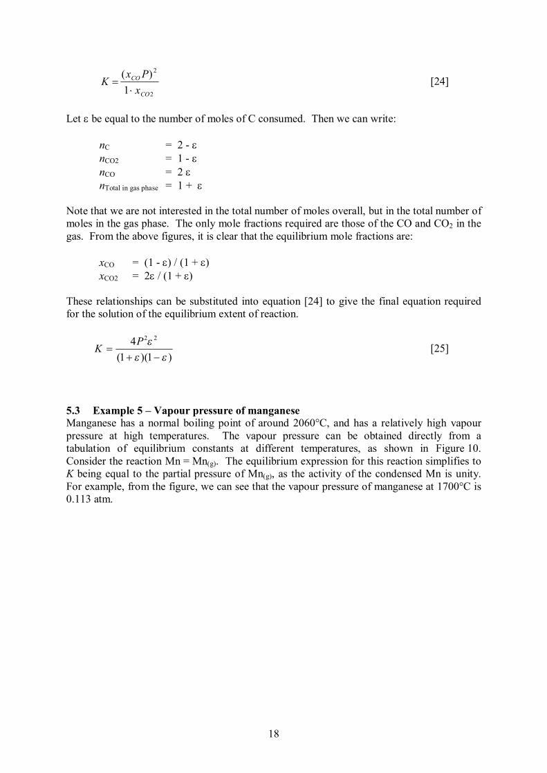
5.3 Example 5 – Vapour pressure of manganese Manganese has a normal boiling point of around 2060°C, and has a relatively high vapour pressure at high temperatures. The vapour pressure can be obtained directly from a tabulation of equilibrium constants at different temperatures, as shown in Figure 10. Consider the reaction Mn = Mn(g). The equilibrium expression for this reaction simplifies to K being equal to the partial pressure of Mn(g), as the activity of the condensed Mn is unity. For example, from the figure, we can see that the vapour pressure of manganese at 1700°C is 0.113 atm.

19

Figure 10: Tabulation of vapour pressure of manganese (shown as K)

5.4 A word of caution It has been noted that the equilibrium constant is a function of temperature only, but the equilibrium composition of a given system depends on the starting composition (in terms of the total number of moles of each element present) and the pressure as well. For this reason, great care should be taken before extrapolating results from one ‘equilibrium curve’ to another situation.

6 FREE-ENERGY MINIMIZATION Pyrometallurgical processes take place at high temperatures. For this reason, the attainment of equilibrium in many processes is not prevented by kinetic limitations. However, a general method for the prediction of the composition of an isothermal multiphase system at equilibrium is required. Problems relating to the chemical equilibrium of a system involving several chemical species are notoriously intractable, requiring the solution of many simultaneous non-linear equations. However, such problems can be reduced to the minimization of the Gibbs free energy of the system, which is the fundamental description of chemical equilibrium. In general, there is an infinite number of ways in which non-negative mole numbers can be assigned to the possible product species such that the chemical reactions involving the specified reactants will be balanced. At a specified temperature and pressure, the most stable products (the desired solution to the problem) are those associated with the lowest free energy. The equilibrium state of a closed system is that for which the total Gibbs free energy is a minimum with respect to all possible changes at the given temperature and pressure.

20

This criterion of equilibrium provides a general method for the determination of equilibrium states. One writes an expression for the total Gibbs free energy of the system as a function of the number of moles of the components in the several phases, and then finds the set of values for the number of moles which minimizes this function, subject to the constraints of mass conservation. This procedure can be applied to problems of phase or chemical-reaction equilibria or to a combination of both. The technique has the advantage of requiring little chemical intuition or experience to set up and carry out the necessary calculations. The foremost proponent of this approach is undoubtedly Eriksson5-7. He has developed a technique for solving the equilibria in systems containing one gas phase, several pure condensed phases, and several condensed mixtures. 6.1 Fundamental relationships In the following derivation, it is assumed that the gas phase is ideal and that the condensed phases are immiscible. Elimination of this second assumption, which may be necessary in some systems having large liquid fractions, requires a more advanced mathematical treatment. The Gibbs free energy (G) of a multiphase multicomponent system can be expressed as

∑∑=i

pi

pi

pnG µ [26]

where:

G = Gibbs free energy of the system (kJ) pin = number of moles of species i in phase p (mol)

piµ = chemical potential of species i in phase p (kJ/mol)

The chemical potential is defined as

pi

oi

pi aRT ln+= µµ [27]

where:

oiµ = reference (standard state) chemical potential of species i (kJ/mol)

R = ideal gas constant = 8.3143 J mol-1 K-1 T = absolute temperature (K)

pia = activity of species i in phase p

It is convenient to (arbitrarily) set o

iµ = 0 for all elements in their standard states. Then for all species

ofi

oi G∆=µ [28]

where

ofiG∆ = Gibbs free energy of formation of species i at the process temperature

(kJ/mol)

21

Therefore

pi

ofi

pi aRTG ln+∆=µ [29]

The gas phase is assumed to behave ideally. Therefore, for the gaseous species, the activities ( g

ia ) are equal to the partial pressures. That is to say, the activity of a particular species is equal to its mole fraction times the total pressure.

PNna ggi

gi ⋅= )/( [30]

where:

gin = number of moles of species i in the gas phase

Ng = total number of moles in the gas phase P = total pressure of the system (atm)

For the species in condensed mixtures (which are non-ideal in the general case), the activities are expressed as

)/( ppi

pi

pi Nna ⋅= γ [31]

where:

piγ = activity coefficient of species i in condensed mixed phase p pin = number of moles of species i in condensed mixed phase p

Np = total number of moles in the condensed phase 6.2 Function to be minimized This minimization problem has the free energy of the system as the objective function, and the number of moles of each of the chemical species in each phase as the variables. The total Gibbs free energy (G) of the system can be expressed in dimensionless form by dividing G by RT. This function is shown in equation [32]. The phases are numbered consecutively, from p = 1 for the gas phase, via p = 2 to (q + 1) for the condensed mixtures, up to p = (q + s + 1) for the condensed pure phases. The total number of moles in phase p is denoted by Np, and the total number of species present in phase p is denoted by mp.

∑∑∑=

+

==

++

∆+

++

∆=

pm

ip

pip

i

pi

ofp

i

q

p

iiof

m

ii N

nRTG

nNn

PRTG

nRTG

1

1

21

11

1

1 lnln)(

lnln)(1

γ

∑∑=

++

+=

∆+

pm

i

pi

ofp

i

sq

qp RTG

n1

1

2

)(

[32]

22

where: G = total Gibbs free energy of the system (kJ) R = ideal gas constant = 8.3143 J mol-1 K-1 T = absolute temperature (K)

pin = number of moles of species i in phase p (mol)

pi

ofG )(∆ = Gibbs free energy of formation of species i at the process temperature

(kJ/mol) P = total pressure (atm)

piγ = activity coefficient of species i in phase p

Determination of the equilibrium composition requires finding a non-negative set of mole numbers p

in that will minimize the total free energy of the system. 6.3 Constraining equations Although molecular species are not conserved in a closed reacting system, the amounts of each element present remain constant. Therefore, the constraints that apply are those of mass conservation for each element present in the system, as well as those of non-negativity of the number of moles of each species present. Each element is conserved in the process, so that

∑∑=

++

=

=pm

ij

piij

sq

pbna

1

1

1

(j = 1, 2, …, l) [33]

where:

aij = number of atoms of element j in species i bj = total number of moles of element j in the feed l = total number of elements present in the system

6.4 Optimization method The optimization method (explained in detail elsewhere8) involves a search for a minimum value of the dimensionless quantity (G/RT), subject to the mass balance relations as subsidiary conditions. The standard solution to this type of problem involves the use of undetermined Lagrange multipliers. These are artificial variables which are used in constrained optimization problems to avoid the need for explicit simultaneous solution of a given function and its constraining function.

7 SOLUTIONS A solution is a homogeneous mixture of two or more substances, and is a single phase. Gas mixtures, molten slags, metals, alloys, mattes, speisses, and salts are metallurgically important solutions. A component of a solution can take part in reactions in the same way as a pure substance can; however, its activity (that active portion able to react) is related to the concentration in the solution, and to the effect of the other constituents of the solution upon it.

23

The activity of a component is equal to its mole fraction multiplied by an activity coefficient. An ideal solution is one having all activity coefficients equal to one; i.e. activities are equal to mole fractions. In equilibrium calculations, it is assumed that the activity of each species in the specified system can be calculated from the chemical composition of each phase. The activity of a component in a solution is defined as the ratio of its fugacity to its standard-state fugacity. The activity function can, at least in theory, be calculated from the equation of state of the solution. However, because of the low accuracy of liquid-phase equations of state in general, other techniques are required for the calculation of activities in slag and metal solutions. Unfortunately, accurate activity data for the components in complex slags and metals remains limited, but is steadily improving. The ideal-solution model, in which the activity of each component equals its mole fraction, is the simplest model of activities in solution. This model takes into account only the effect of dilution on activities, and ignores the chemical and physical effects of mixing. Although very few metal solutions, and even fewer oxide systems, display ‘ideal’ behaviour, this is chosen as the reference for solution behaviour. It is usually expedient to assume that the gas phase behaves ideally, as this is a reasonably accurate assumption under the conditions most frequently encountered (namely low pressure and high temperature). Slags are relatively concentrated solutions of oxides, and usually contain oxides such as SiO2, CaO, MgO, and Al2O3, together with the oxides of the metals involved in the process. They are complex solutions in which each component influences the activity of the others, and hence their behaviour is not easily described. Some authors have derived solution models for slags based on the ideal or regular constitutional models, using various species as components. Others have adopted a structural approach, modelling the slag properties in terms of some hypothetical structure. It is now generally accepted that slags are essentially ionic systems, although they have on occasion been viewed as having a molecular structure, with the molecules envisaged as combining to form more complex (and unreactive) molecular structures, for example, 2CaO.SiO2, which exist in dissociated equilibrium with the corresponding components. 7.1 Ideal Mixing of Complex Components A major improvement on the ideal-mixing model is the use of the Ideal Mixing of Complex Components9 (IMCC) approach, as proposed by Hastie and Bonnell10-12. This generally allows good estimates for the equilibrium products to be generated, by including many possible intermediate compounds in the list of species assumed to be present at equilibrium; in this way it models some of the chemical interactions between the species. This model attributes deviations from ideal-solution behaviour to the formation of complex component liquids and solid phases. The activities are taken to be equal to the equilibrium mole fractions of the uncomplexed components. Although this solution model may be fictitious, it provides a useful starting point, in the absence of a better model for complex systems. One of the prime benefits of this predictive model is that it is equally capable of handling systems containing few or many components.

24

The IMCC approach has been used previously9 to model simple industrial slags. Figure 11 shows the activity – mole-fraction relationship for MgO in the CaO-MgO-SiO2 ternary system at a constant level of 30 mole % CaO. From the figure, a comparison can be made between the calculated activities, the experimentally determined activities, and the ideal activities. There was excellent agreement between the calculated and experimentally determined activities of CaO and MgO, and reasonably good agreement between the activity curves for SiO2. It is also important to note the large discrepancies that would result if the assumption of an ideal solution was made.

Figure 11: Activity – mole-fraction curve for MgO in the system CaO-MgO-SiO2 (at

30% CaO) at 1600°C The IMCC model is a good starting point for modelling unknown systems, but if there is sufficient data available, it may be better to use one of the more sophisticated solution models described below. There are two most prominent solution models being actively developed for multi-component slag systems, and one for alloy systems.

25

7.2 Cell model for slags The cell model13-14, as proposed by H. Gaye of IRSID, France, and others, describes steelmaking slags as having both anionic and cationic sub-lattices. The cell model uses data derived from binary systems to describe higher-order systems. This has led to some limitations, particularly in systems with a high content of alumina. 7.3 Modified quasichemical model for slags The modified quasichemical model15 developed by A.D. Pelton and M. Blander is the subject of vigorous ongoing work at the École Polytechnique in Montreal, Canada. Solution data for an ever-increasing variety of multi-component systems is being evaluated, and the models extended. These models are available as part of the F*A*C*T database16-17. The modified quasichemical (MQ) model was developed for the analysis of the thermodynamic properties of structurally ordered liquid solutions, particularly molten silicates. Ternary and quaternary properties are estimated from the subsidiary binary systems. The MQ model is not intended as a detailed theory of silicate structure, but rather as a mathematical formalism which has the advantage of generality and which appears to have the charateristics required for relatively reliable interpolations and extrapolations of data into unmeasured regions, and for extensions which can be used for multi-component systems. 7.4 Modified interaction parameter model for alloys The modified interaction parameter model18, developed by A.D. Pelton and C.W. Bale is currently the best available for a wide range of alloys, including those based on Fe, Cu, Al, Ni, and Pb. These models are also available as part of the F*A*C*T database. Because the unified interaction parameter formalism is thermodynamically self-consistent at both infinite dilution and finite concentrations, and it unifies various other formalisms for which older data is available, it has become the most widely used formalism for estimating activities of components in liquid alloys. However, some care should be taken in the application of data derived from experiments on dilute alloys (e.g. steel) to concentrated alloys (e.g. ferrochromium).

8 CONCLUSIONS The laws of thermodynamics provide an elegant mathematical expression of some empirically-discovered facts of nature. The principle of energy conservation allows calculations to be made of the energy requirements for processes. The principle of increasing entropy (and the resulting free-energy minimization) allows predictions to be made as to the extent to which those processes may proceed. Readily-available software allows thermodynamic calculations to be performed quickly and consistently. Using a reference state of the elements in their standard state at 25°C and 1 atm. having a standard enthalpy of formation of zero, energy balance calculations can be carried out without reference to the process or reaction paths. Equilibrium calculations can be performed most effectively using the technique of free-energy minimization. The equilibrium state of a closed system is that for which the total Gibbs free energy is a minimum with respect to all possible changes at the given temperature and pressure. This criterion allows the calculation of the equilibrium state of multiple

26

simultaneous chemical reactions, simply requiring the specification of the amounts of material initially present, the temperature and pressure of the system, and a list of possible species in each phase. A good solution model should be capable of giving not only a good description of the available experimental data, but also reasonable extrapolations in temperature and to higher-order systems. A number of good solution models for slags and alloys are available, but this is still an area of active development.

9 REFERENCES 1. G.M. Barrow, “Thermodynamics should be built on energy – not on heat and work”,

J.Chem.Educ., February 1988, Vol.65, No.2, pp.122-125. 2. C.P. Snow, “The two cultures and a second look”, Cambridge University Press, 1964,

p.15. 3. M.L. McGlashan, The use and misuse of the laws of thermodynamics”,

J.Chem.Educ., May 1966, Vol.43, No.5, pp.226-232. 4. W.F. Harris, “The plethora of equilibrium constants”, ChemSA, November 1978,

pp.170-172. 5. G. Eriksson, “Thermodynamic studies of high temperature equilibria. III. SOLGAS, a

computer program for calculating the composition and heat condition of an equilibrium mixture”, Acta Chem. Scand., Vol.25, 1971, pp.2651-2658.

6. G. Eriksson & E. Rosen, “Thermodynamic studies of high temperature equilibria. VIII. General equations for the calculation of equilibria in multiphase systems”, Chem. Scr., Vol.4, 1973, pp.193-194.

7. G. Eriksson, “Thermodynamic studies of high temperature equilibria. XII. SOLGASMIX, a computer program for calculation of equilibrium compositions in multiphase systems”, Chem.Scr., Vol.8, 1975, pp.100-103.

8. R.T. Jones, “Computer simulation of process routes for producing crude stainless steel”, MSc(Eng) Dissertation, University of the Witwatersrand, Johannesburg, 3 October 1989.

9. R.T. Jones & B.D. Botes, “Description of non-ideal slag and metal systems by the intermediate-compound method”, Proceedings of Colloquium on Ferrous Pyrometallurgy, SAIMM, Vanderbijlpark, 18 April 1989.

10. J.W. Hastie & D.W. Bonnell, “A predictive phase equilibrium model for multicomponent oxide mixtures: Part II. Oxides of Na-K-Ca-Mg-Al-Si”, High Temp. Sci., Vol.19, 1985, pp.275-306.

11. J.W. Hastie, W.S. Horton, E.R. Plante, & D.W. Bonnell, “Thermodynamic models of alkali-metal vapor transport in silicate systems”, High Temp. High Press., Vol.14, 1982, pp.669-679.

12. J.W. Hastie & D.W. Bonnell, “Thermodynamic activity predictions for molten slags and salts”, Abstract, Third International Conference on Molten Slags and Glasses, University of Strathclyde, Glasgow, 27-29 June 1988, The Institute of Metals.

13. H. Gaye, “A model for the representation of the thermodynamic properties of multi-component slags”, University of Strathclyde, Metallurgy Department, Centenary Conference, June 1984, pp.1-14.

14. H. Gaye & J. Welfringer, Proc. 2nd International Symposium on Metall. Slags and Fluxes, Ed. by H.A. Fine and D.R. Gaskell, Lake Tahoe, Nevada, AIME Publication, 1984, p.357.

27

15. A.D. Pelton & M. Blander, Proc. 2nd International Symposium on Metall. Slags and Fluxes, Ed. by H.A. Fine and D.R. Gaskell, Lake Tahoe, Nevada, AIME Publication, 1984, p.281-294.

16. Thermfact, 447 Berwick Avenue, Mont-Royal, Quebec, Canada, H3R 1Z8. 17. W.T. Thompson, C.W. Bale, A.D. Pelton, “Interactive computer tabulation of

thermodynamic properties with the F*A*C*T system”, Journal of Metals, December 1980, pp.18-22.

18. A.D. Pelton & C.W. Bale, Met. Trans., 21A(7), 1990, pp.1997-2002.

28

About the author:

Rodney Jones has worked in the Pyrometallurgy Division at Mintek since 1985. He holds a BSc(Eng) degree in chemical engineering from Wits University, a BA degree in logic and philosophy from the University of South Africa, and a MSc(Eng) degree in metallurgy from Wits University. He is a registered Professional Engineer, a fellow of SAIMM and SAIChE, and a full member of the CSSA. He was a Visiting Professor at the Center for Pyrometallurgy, University of Missouri-Rolla, during July and August 1996,

and a Visiting Research Associate at Murdoch University, Western Australia, between March and May 2002. His main research interests are in the field of computer simulation and design of high-temperature processes, and the development of thermodynamic software. He is also the author of Pyrosim software, for the steady-state simulation of pyrometallurgical processes, in use at 78 sites in 20 countries around the world.