RTFDDA-SCIPUFF

Coupled Applications

Jeff Copeland

and

Rong-Shyang Sheu

Dispersion Models andModeling

• Nature of the problem

• Types of Models

• SCIPUFF

Turbulence and Diffusion - the study of motions

that lead to mixing in a fluid

(not what I’ll talk about)

Transport and Dispersion - the application of

T&D science to study materials that get mixed

in a fluid

(what I’ll try to focus on)

What is meant by T&D

Nature of the Problem

• Purpose

– Regulatory, Emergency response

• Release Mechanics

– Point, line, area

– Instantaneous, continuous

• Type of material

– Gas, aerosol, particulate

• Atmospheric Conditions

– Stability, flow regime

– Knowledge

What are we simulating

Snapshot

Time average

Complexity

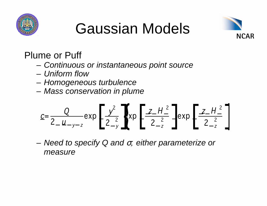
Gaussian Models

Plume or Puff– Continuous or instantaneous point source– Uniform flow– Homogeneous turbulence– Mass conservation in plume

_c=Q

2_ _u _y_z

exp[_ y2

2_y2]{exp[__z_H _2

2_z2 ]_exp[_ _z_H _2

2_z2 ]}

– Need to specify Q and , either parameterize or

measure

Gaussian Models

Advantages– Analytic– Fast– Regulatory

Disadvantages– Simplified

physics– Limited

applicability ofdesignassumptions

Parameterized

Lagrangian Models

• Stochastic model of Lagrangian velocities (Monte-Carlo,Markov-chain)

• Material treated as a cloud of particles that move with themean wind plus a random component based on theturbulence strength

dX

dt=U =U_U

'

U t__ t

'=aU t

'__t_1_a

2_1/2

_t

a=exp___ t

TL_

–t generally given by

x,

y, or

z

–t is a dimensionless random variable with mean of 0 and variance of 1

– TL is the integrated Lagrangian time scale

Lagrangian Models

Advantages– Modifications for

inhomogeneous turbulence

and wind field

– Complicated

sources/releases

– Treatment of buildings

reasonably simple

Disadvantages– Number of particles

(runtime, concentration)

Additional conservationequations added tomesoscale or LESmodels

Advantages– Detailed physics

– Chemistry

Disadvantages– Resolution vs compute

time

Eulerian Models

Hybrid Models

Langrangian-Eulerian

Langrangian-Puff: SCIPUFF

T&D in RAL

• NSAP projects– ATEC, DARPA, DHS, GCAT,…

• Wind Models– RTFDDA

– VDRAS/VLAS

– QUIC-Urb mass conserving flow distortion

– CFD-Urban RANS

• Plume Models– HPAC SCIPUFF Lagrangian-Puff

– CALPUFF Lagrangian-Puff

– QUIC-Plume Lagrangian Particle

– AERMOD Gaussian Plume

What is SCIPUFF

• A Lagrangian-Puff transport and diffusion

model for atmospheric dispersion

applications

– Computes concentration mean and variance

– Wide range of CBRN release plume

applications

– Industrial air pollution studies

– Forest fire plume studies

SCIPUFF Modes

• Stand-alone SCIPUFF that runs on all platforms– Not building aware

– Good for operational range use

– Can be the back-end engine for GUI and web-basedcoupled applications (e.g., Jvis, GCAT, GMOD)

• A component in PC-Windows based HPAC– GUI-based model setup

– Detailed source models

– Display

• Planned integration into JEM

GCAT SCIPUFF interface

HPAC GUI

Requirements for stand-alone

SCIPUFF

• Configuration files that describe

– general information regarding calculation

domain, simulation duration, time step, output

frequency, source material properties

– Description of meteorological data and

surface characteristics

– Source terms, location, release type, amount

(or strength), duration

Meteorology Input

• One or more surface and/or upper-airobservations– U, V (minimum required input)

– Stability related variables (T, PGT, MOL)

– Turbulence related variables (PBL height, sensibleheat flux)

• Gridded model output from 4DWx systems– Height level, terrain, fixed lat/lon intervals

– U, V, W, temperature

– Terrain, PBL height, sensible heat flux

– Uncertainty in U, V fields

– Grid nesting capable

SCIPUFF Output

• Surface dosage file

• Surface deposition file

• Puff file, from which concentrations can be

extracted

• Statistical quantities (mean and variance)

Coupled SCIPUFF

Example 1

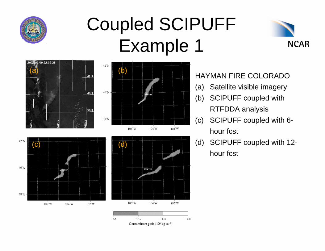
HAYMAN FIRE COLORADO

(a) Satellite visible imagery

(b) SCIPUFF coupled with

RTFDDA analysis

(c) SCIPUFF coupled with 6-

hour fcst

(d) SCIPUFF coupled with 12-

hour fcst

(a) (b)

(c) (d)

Coupled SCIPUFF

Example 2(a)

(b)

DP26

Range scale

(a) SCIPUFF driven by observations

(b) SCIPUFF coupled with RTFDDA