&rpsxwhu dlghgghvljq &$' &rpsxwhu … · issn 1453 – 7303 “hidraulica” (no....
TRANSCRIPT

Computer-aided design (CAD)Computer-aided engineering (CAE)
Computer-aided manufacturing (CAM)
No. 2

ISSN 1453 – 7303 “HIDRAULICA” (No. 2/2019) Magazine of Hydraulics, Pneumatics, Tribology, Ecology, Sensorics, Mechatronics
3
CONTENTS
EDITORIAL: Research for snails Ph.D. Petrin DRUMEA
• Heavy Duty Machine Tools - Specific Pneumatic Drives Prof. PhD Eng. Anca BUCUREȘTEANU, Prof. PhD Eng. Dan PRODAN, Assoc. Prof. PhD Eng. Adrian MOTOMANCEA
6 - 15
• Modeling the Equipment Shape of the Technological Flow of the Waste Water Treatment Station
Prof. PhD.eng. Mariana PANAITESCU, Prof. PhD.eng. Fănel-Viorel PANAITESCU, PhD. Ileana-Irina PANAITESCU
16 - 22
• Researches Regarding the Execution of a Flat Jet Generator Used for Water Aeration
PhD Student Nicoleta Dorina ALBU, Prof. Dr. Eng. Nicolae BĂRAN, PhD Student Mihaela PETROȘEL, Sl. Dr. Eng. Daniel BESNEA, Sl. Dr. Eng. Mihaela CONSTANTIN
23 - 28
• Study of Mass Water Oscillations and Water Hammer Occurrence in Hydraulic Installations
Assoc. Professor PhD Sanda BUDEA
29 - 35
• Fluid Flow within a Hydrostatic Lobe Pump Assistant professor Fănel Dorel ȘCHEAUA
36 - 42
• Sensitivity Analysis of Sharp-Crested Weirs as a Function of Shape Opening, for Small Discharges
Assoc. Prof. Cristina Sorana IONESCU, Assoc. Prof. Daniela Elena GOGOAŞE NISTORAN, Assoc. Prof. Ioana OPRIŞ, Assist. Ștefan-Mugur SIMIONESCU
43 - 51
• From Human-Environment Interaction to Environmental Informatics (IV): Filling the Environmental Science Gaps with Big Open-Access Data
Assoc. Prof. eng. Mirela COMAN, PhD stud. Bogdan CIORUȚA
52 - 61
• Equipment for Obtaining Thermal Energy by Using Biomass Ph.D. Eng. Gabriela MATACHE, Ph.D. Student Ioan PAVEL, Ph.D. Eng Gheorghe ȘOVĂIALĂ, Dipl. Eng. Alina Iolanda POPESCU, Ph.D. Student Eng. Mihai-Alexandru HRISTEA.
62 - 71

ISSN 1453 – 7303 “HIDRAULICA” (No. 2/2019) Magazine of Hydraulics, Pneumatics, Tribology, Ecology, Sensorics, Mechatronics
4
BOARD
MANAGING EDITOR
- PhD. Eng. Petrin DRUMEA - Hydraulics and Pneumatics Research Institute in Bucharest, Romania
EDITOR-IN-CHIEF
- PhD.Eng. Gabriela MATACHE - Hydraulics and Pneumatics Research Institute in Bucharest, Romania
EXECUTIVE EDITOR, GRAPHIC DESIGN & DTP
- Ana-Maria POPESCU - Hydraulics and Pneumatics Research Institute in Bucharest, Romania
EDITORIAL BOARD
PhD.Eng. Gabriela MATACHE - Hydraulics and Pneumatics Research Institute in Bucharest, Romania
Assoc. Prof. Adolfo SENATORE, PhD. – University of Salerno, Italy
PhD.Eng. Catalin DUMITRESCU - Hydraulics and Pneumatics Research Institute in Bucharest, Romania
Assoc. Prof. Andrei DRUMEA, PhD. – University Politehnica of Bucharest, Romania
PhD.Eng. Radu Iulian RADOI - Hydraulics and Pneumatics Research Institute in Bucharest, Romania
Assoc. Prof. Constantin RANEA, PhD. – University Politehnica of Bucharest; National Authority for Scientific Research and Innovation (ANCSI), Romania
Prof. Aurelian FATU, PhD. – Institute Pprime – University of Poitiers, France
PhD.Eng. Małgorzata MALEC – KOMAG Institute of Mining Technology in Gliwice, Poland
Prof. Mihai AVRAM, PhD. – University Politehnica of Bucharest, Romania Lect. Ioan-Lucian MARCU, PhD. – Technical University of Cluj-Napoca, Romania
COMMITTEE OF REVIEWERS
PhD.Eng. Corneliu CRISTESCU – Hydraulics and Pneumatics Research Institute in Bucharest, Romania
Assoc. Prof. Pavel MACH, PhD. – Czech Technical University in Prague, Czech Republic
Prof. Ilare BORDEASU, PhD. – Politehnica University of Timisoara, Romania
Prof. Valeriu DULGHERU, PhD. – Technical University of Moldova, Chisinau, Republic of Moldova
Assist. Prof. Krzysztof KĘDZIA, PhD. – Wroclaw University of Technology, Poland
Prof. Dan OPRUTA, PhD. – Technical University of Cluj-Napoca, Romania
PhD.Eng. Teodor Costinel POPESCU - Hydraulics and Pneumatics Research Institute in Bucharest, Romania
PhD.Eng. Marian BLEJAN - Hydraulics and Pneumatics Research Institute in Bucharest, Romania
Assoc. Prof. Ph.D. Basavaraj HUBBALLI - Visvesvaraya Technological University, India
Ph.D. Amir ROSTAMI – Georgia Institute of Technology, USA
Prof. Adrian CIOCANEA, PhD. – University Politehnica of Bucharest, Romania
Prof. Carmen-Anca SAFTA, PhD. - University Politehnica of Bucharest, Romania
Assoc. Prof. Mirela Ana COMAN, PhD. – Technical University of Cluj-Napoca, North University Center of Baia Mare, Romania
Prof. Ion PIRNA, PhD. – The National Institute of Research and Development for Machines and Installations Designed to Agriculture and Food Industry - INMA Bucharest, Romania
Assoc. Prof. Constantin CHIRITA, PhD. – “Gheorghe Asachi” Technical University of Iasi, Romania
Published by: Hydraulics and Pneumatics Research Institute, Bucharest-Romania Address: 14 Cuţitul de Argint, district 4, Bucharest, 040558, Romania Phone: +40 21 336 39 91; Fax: +40 21 337 30 40; e-Mail: [email protected]; Web: www.ihp.ro with support from: National Professional Association of Hydraulics and Pneumatics in Romania - FLUIDAS e-Mail: [email protected]; Web: www.fluidas.ro
HIDRAULICA Magazine is indexed by international databases
ISSN 1453 – 7303; ISSN – L 1453 – 7303

ISSN 1453 – 7303 “HIDRAULICA” (No. 2/2019) Magazine of Hydraulics, Pneumatics, Tribology, Ecology, Sensorics, Mechatronics
5
EDITORIAL
Research for snails
Most of the time, the political and economic decision-
makers of the country explain to us quite vigorously that in our
country one of the priority directions of development is scientific
research. This implies either that they do not know what
"priority" means or do not know what "research" means, or they
do not know what's going on in reality. In all cases the
necessary conclusion is that these people must be taken the
right to decide in an area they do not know or, even worse, hate.
Ph.D.Eng. Petrin DRUMEA
MANAGING EDITOR
It is not normal to decide for a country, in a special activity field, people who have not
conducted research activities or not even have used the research results.
In recent years, project competitions under programmes with pompous names have
been launched, with very long deadlines, low values and with many and unnecessary
requirements. To work on a project with a budget amounting to one hundred - two hundred
thousand euros, in a consortium of several research or production partners, for 2 or 3
years is practically a method of slowing down the research activity.
This snail rhythm is not accidental, as it reduces state investment in research
programmes. The method of launching up to 200 projects at 2 or 3 years is a way of trying
to keep a domain that we call priority (only because that's how we heard that things are in
the world) in a lethargic state.
However, it does not seem right that we have introduced the professional training of
any kind and the mobility actions in the core areas of research; the latter ensure the
journeys of some persons who will tell us, possibly at specialized meetings, that intensive
and high-level research is being conducted worldwide. Of course, these subdomains are
necessary, too, but as supporting research, and not as basic elements.
How can small and medium-sized enterprises, emerged in a large number in
Romania, be supported if the programmes are implemented on a long-term and with low
budgets?
A serious, important but unfortunately bad fact is that, in time, the main results of
applied research, industrial research even, have been established to be the scientific
articles, whose international publication has become a business in itself.
The slow moving of research, with predictably modest results, leads to a number of
researchers in a continuous decrease, and the influence of research on national level, in
economic and financial terms, is becoming less and less.
It is possible that I do not understand things anymore, since I am overcome by the
rhythm and modernity of the research policies. Lots of success to everyone!

ISSN 1453 – 7303 “HIDRAULICA” (No. 2/2019) Magazine of Hydraulics, Pneumatics, Tribology, Ecology, Sensorics, Mechatronics
6
Heavy Duty Machine Tools - Specific Pneumatic Drives
Prof. PhD Eng. Anca BUCUREȘTEANU1, Prof. PhD Eng. Dan PRODAN1, Assoc. Prof. PhD Eng. Adrian MOTOMANCEA1
1 University POLITEHNICA of Bucharest, [email protected], [email protected], [email protected]
Abstract: This paper introduces some applications of the pneumatic drives for heavy duty machine tools. Only the machine pneumatic drives proper are presented, not their associated devices too. These applications are used for heavy duty machine tools like centre and vertical lathes, gantry type milling machines, boring and milling machines and horizontal boring and milling machines. The pneumatic systems presented hereby are an independent part of the machine since the manufacturing stage of this one or they have been attached to the machine during its remanufacturing. They are formed of typified elements mostly, supplied by specialized manufacturers.
Keywords: Machine tools, pneumatic drives, auxiliary pneumatic chains with pneumatic actuation
1. Introduction
Almost every factory or workshop is equipped with central compressor stations and compressed air distribution networks. Therefore, it is necessary to design and build modern pneumatic systems of high productivity. The most important advantages of the pneumatic drives that favored their use in machine tools building also are listed below: • Achievement of clamping constant forces whose value can be easily controlled during
operation; • Accurate establishment of the developed forces value and the constant maintaining of these
ones in order to make possible the machining of semi-finished products with thin and easily deformable walls without the danger of destroying them during the clamping;
• It is easier to maintain and operate the pneumatic drives than the hydraulic systems which are replaced – wherever possible – by the pneumatic drives;
• compatibility with the hydraulic systems within the hydro-pneumatic units, such as in the case of pressure intensifiers;
• possibility to ensure the cooling of the semi-finished products and tools during the cutting operations;
• the motors and devices included in the pneumatic drives are generally normalized components, leading to design labor savings and reduced cost price.
The heavy duty machine tools, by their intended use and construction, are generally equipped with main and feed kinematic chains electromechanically driven [1]. These kinematic chains develop large powers, highly accurate adjustable rotational speeds and translation speeds. In most cases, these requirements can not be met by the pneumatic systems. Consequently they can be found in the systems serving the non-generating kinematic chains [1] usually named auxiliary kinematic chains.
2. Pneumatically driven safety systems for operator and machine
In the case of the heavy duty vertical lathes [1, 2, 3] with table diameter larger than 1400mm, depending on their destination, these ones can be provided with safety covers that separate the work area from the machine outside. It is possible to have two or three covers. Their number is determined depending on the size of the machine and on the way the machine is fed with semi-finished materials. Generally, these covers have pneumatic actuation. They can be actuated independently or not, by manual control or by the machine program. Other specific requirements of these covers are listed below:

ISSN 1453 – 7303 “HIDRAULICA” (No. 2/2019) Magazine of Hydraulics, Pneumatics, Tribology, Ecology, Sensorics, Mechatronics
7
- their steady locking in upper position; - prevention measures against accidental drop if the pressure supply fails; - if it is the case, synchronous travel with the cross-rail. Figure 1 presents the pneumatic diagram of the system that runs the two covers of a vertical lathe SC17 type.
Fig. 1. Pneumatic diagram for the actuation of the covers of the vertical lathe SC17 type
The unit is connected to the pneumatic source 1 by actuating the manual selector 3. The electric control is started by means of the electric valve 4 (E0 powered). The compressed air is filtered and enriched with oil drops by the preparation group 6. The operating pressure (maximum 5 bar) is regulated by means of the pressure regulator 7. The value of the operating pressure is read on the manometer 8 while the pressure switch 9 confirms the presence of pressure in the unit. The check valves 10 and the electric valves 11 are assembled on the plate 5. These valves supply the two cylinders (CL- left side, CR –right side) 13 through the agency of the pneumatic pilot valve 12. The positions of the two cylinders are confirmed by the position limit stops L1-L4, 14. The noise during operation is reduced by means of the dampers 2 [4, 5, 6]. By actuating the electromagnets E1-E4 it is possible to move the cylinders CL and CR upwards and downwards, simultaneously or not. The commanded positions are confirmed by the limit stops L1-L4. If the electric valves E1-E4 did not receive any commands, the valves 12 with pneumatic actuation will lock the cylinders so that the accidental fall of the covers will be prevented. The check valves 10 ensure the independent operation of the two cylinders by impeding the re-entry of the eliminated air into the circuit. The cylinders are provided with braking systems at stroke end in both directions of the stroke. Figure 2 shows a part of the pneumatic unit [5].
Fig. 2. Part of the pneumatic unit

ISSN 1453 – 7303 “HIDRAULICA” (No. 2/2019) Magazine of Hydraulics, Pneumatics, Tribology, Ecology, Sensorics, Mechatronics
8
In the manufactured unit, the pressurization system of the scales on X and Z axes of the machine is also supplied from the pressure intake port 1; this system is not represented in the diagram shown in Figure 1. The notations are the same as in Figure 1. In Figure 3 is shown the pneumatic diagram for the actuation of the covers of the lathe SC33 CNC type. There are three covers for the bed, actuated by the cylinders CL, CC and CR 13 but also a 90o rotary cover at the disk type tool magazine. This cover is driven by the pneumatic oscillating motor 17 [5, 6].
Fig. 3. Pneumatic diagram for the actuation of the covers of a vertical lathe SC33CNC type
The elements numbered from 1 to 14 in Figure 3 have the same significance as the ones in Figure 1, with the remarks below: - valves 12 have another diagram, - there are 13 check valves 10, - there are three lifting cylinders: one on the left CL, one in the centre CC and one on the right CR. Some additional elements are shown in Figure 3: 15 – check valves to avoid the depressurization, 16-electric valve for exhausting the air from the cylinders CL and CR if the left side and right side covers are pushed downwards by the cross-rail; in this case, the cover driven by the central cylinder CC is fully lifted, 17 – throttle valve for the adjustment of the speed of descent together with the cross-rail, 18- oscillating pneumatic motor with braking at stroke ends. The operation of the unit is similar to the one of the SC17 lathe. The essential difference is given by the fact that if the cross-rail of the lathe goes downwards for positioning or as work axis, the covers actuated by the left side cylinder CL or by the right side cylinder CR are pushed downwards by the cross-rail while the central cover keeps its position. When the cross-rail went downwards until the upper level of the side covers, the electromagnet E9 of the electric valve 16 will be actuated. The cross-rail presses the cylinders CL and CR eliminating the air from the chambers A of these cylinders through the throttle 17. The chambers B of the cylinders suck the atmospheric air through the valves 15. The electric valve 16 is not actuated for the movements upward and downward of the covers. The tool magazine with 12 stations is located on the right side of the cross rail and is protected by a tiltable door driven by the rotary pneumatic motor (CPO) 18. This motor is actuated by the electromagnets E7 and E8. The positions of closed / open cover are confirmed by the limit stops L7 and L8. The supply point on the plate 5 can also feed other pneumatic consumers of the machine, such as the tool blowing system, the clamping systems etc. In this case, the unit must meet the following conditions: - the pressure source must cope with the maximum consumption; - consumers must operate at a single pressure adjusted by means of regulator 7;

ISSN 1453 – 7303 “HIDRAULICA” (No. 2/2019) Magazine of Hydraulics, Pneumatics, Tribology, Ecology, Sensorics, Mechatronics
9
- the size of the construction (the DN) must be properly dimensioned.
3. Hydro-pneumatic pressure intensifiers used in machine tools
The pressure intensifiers are compact constructions which enable the transformation and intensification of a pneumatically developed pressure into a hydraulic pressure. This pressure can be sent to a consumer under the form of oil flow. Figure 4 presents the operation diagram of a hydro-pneumatic pressure intensifier manufactured by specialized companies [5, 7].
Fig. 4. Hydro-pneumatic intensifier
The system is supplied with compressed air at the maximum pressure p1 = 2÷10 bar on path 1. If the electric valve 2 is not actuated (E is not supplied), the air presses the surface S5 of the piston 4 which is moved to the right in body 3. The piston 5 too is moved to the right in the same time with both piston 6 and spring 7 that moves to the right as well. The left side chamber of piston 6 separates the oil in body 3 from the path A of body 3.This chamber was initially filled with oil by removing the plug 9.The supply pressure on path C of the body 3, through the check valve 11, actuates the pilot 8 by passing it to the position 2. The rod of piston 4 moved on the total travel C1+C2. All this time, the chamber B of body 3 is maintained at the atmospheric pressure p0. If the electromagnet E is powered, the electric valve 2 switches from position 0 to position 1. In this case, the chamber B of the body 3 will be supplied. The piston 4 will move to the left along the stroke C1, where it opposes a resisting force. This one entails the increase of the pressure in chamber B up to the maximum value p1. This pressure changes the status of the pilot 8 which will be switched to status 1. In this case, the pressure p1 will act on path A and the piston 7 on the surface S1, moving to the left. The surface S2 of this one presses the oil and achieves the pressure p2. This one drives the surface S3 of the piston on the whole remaining stroke C2. Meanwhile, the pressure p2 developed in the chamber with oil can be viewed on the pressure gauge 10. If the electric valve 2 is no more actuated, the entire travel to the right will be performed. The piston is returned to the initial position by the spring 7. The command air is evacuated from the right side chamber of the valve 8 in a supervised manner, by means of the throttle valve 10. If the frictions and the possible losses are neglected, the maximum pressure developed in the pneumatic chamber has the value:
𝑝2 = 𝑝1𝑆1
𝑆2 (1)
The maximum forces developed at the rod of cylinder 4 along the two strokes C1 and C2 are shown below:

ISSN 1453 – 7303 “HIDRAULICA” (No. 2/2019) Magazine of Hydraulics, Pneumatics, Tribology, Ecology, Sensorics, Mechatronics
10
𝐹1 = 𝑝1𝑆4 (2)
𝐹2 = 𝑝2𝑆3 = 𝑝1𝑆1
𝑆2𝑆3 (3)
The system presented hereby includes the pressure intensifier and the power cylinder joined in a single construction. But there are also some hydro-pneumatic pressure intensifiers that can serve several cylinders [7]. Figure 5 shows how the four cylinders are supplied. In their case, the stroke C1 and the return along the total stroke C1+C2 are achieved pneumatically. The power stroke C2 is made hydraulically at an intensified pressure.
Fig. 5. Hydro-pneumatic intensifier that serves four cylinders
The hydro-pneumatic intensifier supplies the cylinders 2 through the valves 3 during the phases of approach (C1) and retreat (C1+C2). During the phases that require high forces, stroke (C2), the cylinders are hydraulically supplied by means of the valves 4. The silent operation is ensured by the noise suppressor 5. The hydro-pneumatic pressure intensifiers can provide a pneumatic pressure p1 = 2÷6 bar and hydraulic pressures up to p2 = 400 bar. In the field of heavy duty machine tools, these intensifiers are used as systems for unloading the guideways [1, 8]. The sliding guideways enable the unloading of big loads, the accurate stop and locking on a commanded position. As for the heavy duty machine tools, the rolling guideways are preferred for the achievement of long travels. The rolling guideways are characterized by higher speeds and lower resisting forces. By using combined guideways and unloading systems, we can obtain systems that make possible positioning movements at high velocity on almost the entire travel; afterwards, the travel is made at lower velocity, on the sliding guideways only, followed by accurate stop and possible locking of axis [1, 2]. Figure 6 shows the operating principle of the unloading systems [8].
Fig. 6. Hydraulic system for guideways unloading

ISSN 1453 – 7303 “HIDRAULICA” (No. 2/2019) Magazine of Hydraulics, Pneumatics, Tribology, Ecology, Sensorics, Mechatronics
11
The saddle 2 travels on the guideways of the bed 1, with the frictional coefficient μ1. The tougher plates 3 too are located on the bed. The intermediate elements 6 (with rollers) are introduced between these plates. The rolling frictional coefficient μ2 occurs between the rollers and the plates 3. If the supply pressure p is missing, the system will operate without unloading. If there is a pressure p in the n pistons 4, with the active surfaces S, these ones press the elements 6 on the plates 3. The effect of the pressure action is the taking over of a part of the load G by the rolling guideways. The guideways are secured (closed) by the closing plates 5. On the lower part of these plates there are insertions of anti-friction material 7. In both cases, the force F required at the level of the final element of the feed device 8 will have the expressions as follows: - without unloading
𝐹 = 𝜇1𝐺 (4)
- with unloading
𝐹 = 𝜇1𝑁1 + 𝜇2𝑁2 (5)
The following notations were used in the relation (5): N1 - normal force at the sliding guideways level, N2 - normal force at the rolling guideways level. These forces have the expressions:
𝑁1 = 𝐺 − 𝑁2 (6)
𝑁2 = 𝑛𝑝𝑆 (7)
The value of pressure p is so adjusted as to ensure a sufficient unloading at the associated kinematic chain but to not reach the total unloading, characterized by the critical value:
𝑝𝐶 =𝐺
𝑛𝑆 (8)
Figure 7 presents the dependence of the force (F) developed by the unloading pressure (p).
Fig. 7. Dependence of the force required by the unloading pressure in the kinematic chain
The unloading with a pressure higher than the value pC entails the loss of the sliding guidance, the instability and even the overstress of the closing elements 3 and 5. Once settled the value of the operating pressure p, this one must be ensured and maintained in the n pistons as long as necessary. Usually, the pressure is necessary for the fast travels made for positioning. These travels are performed during much smaller times than the ones required by the machining operations. It is the case of the unloading of the X axes guideways in the gantry type milling machines and the heavy duty boring and milling machines [1]. The hydraulic unloading can be performed in three manners: a- with hydraulic units specially built; b- with hydraulic pressure intensifiers [8]; c- with hydro-pneumatic intensifiers. Generally, the hydraulic units intended for the unloading provide pressures of 250 bar. Higher values of the pressure involve the use of more expensive components. Figure 8 shows the hydraulic diagram and some of the hydraulic elements used to unload the guideways of a horizontal boring and milling machine.

ISSN 1453 – 7303 “HIDRAULICA” (No. 2/2019) Magazine of Hydraulics, Pneumatics, Tribology, Ecology, Sensorics, Mechatronics
12
a. b.
Fig. 8. Hydraulic system for the unloading of X axis guideways The pump 4 actuated by the electric motor 3 sucks the oil from the tank 1 through the suction filter 2. The maximum operating pressure is adjusted by means of the pressure relief valve 5. Afterwards the oil is filtered by means of the filter with clogging indicator 6. The adjusted pressure is read on the pressure gauge 7. The plate 14 is supplied on the path P. The electric valve 12 and the check valve hydraulically operated 13 are located on the plate 14. The actuation of the electromagnet E2 leads to the charge of the circuit for guideways unloading. The pressure adjusted at the pressure relief valve 5 is ensured for all the n unloading cylinders 15. At this moment the pump can be stopped. The accumulator helps to maintain the pressure between the values adjusted at the pressure switches 8.1 and 8.2. The pressure switch 8.1 commands the eventual re-start of the pump, while the pressure switch 8.2 will command the stop of the pump. All this time, the pressure can be viewed on the pressure gauge 11. Regardless of whether the pump is running or not, the system will be discharged by actuating the electromagnet E1. The hydraulic unit includes quite many elements and the power consumed by these ones is about 3KW. If a higher pressure is needed, hydraulic pressure intensifiers [4, 6, 7] shall be used. In this case, the hydraulic diagram includes one or several intensifiers besides the elements used above. The use of the hydro-pneumatic intensifiers simplifies very much the construction. The pump, the electric motor and many components are eliminated. In this case, if a maximum number of 6 cylinders is needed, it is possible to use a unit similar to the one shown in Figure 4. The ordinary hydraulic diagrams use elements that run at pressures of 320 bar at the most. In case of higher pressures, the coupling elements (pipes, hoses, fittings) are special, much more expensive than the usual ones. Another advantage of the hydro-pneumatic pressure intensifiers is the fact that the oil tank, the filtering unit etc. are no more needed.
4. Balancing pneumatic systems
The balancing systems are used for the feed kinematic chains that operate vertically, in order to reduce the necessary power and to avoid the oversizing of the basic components (electric motor, reducer, screw and ball nut mechanism). These systems operate in parallel with the feed kinematic chain but take over a part of the weight of the live elements G [1, 9]. Depending on how they perform this function, the balancing kinematic chains can be mechanical (with counterweight), hydraulic or pneumatic ones. The mechanical ones have a simpler structure but they involve the increase of the machine mass, require specific safety systems and they diminish the performances of the kinematic chain, especially in transitory regime. The hydraulic systems are efficient, do not increase the mass of the machine, ensure a proper dynamic behavior of the feed dynamic chain but they also involve the

ISSN 1453 – 7303 “HIDRAULICA” (No. 2/2019) Magazine of Hydraulics, Pneumatics, Tribology, Ecology, Sensorics, Mechatronics
13
presence of a complex hydraulic unit with generally expensive hydraulic elements. Another disadvantage is the need of large oil tanks (required by the high installed power) and, in some cases, cooling systems for the oil. The pneumatic balancing can be used for smaller travels than the ones of the hydraulic systems; it also can be used when it is possible to balance the movable weight by means of one or two cylinders of acceptable size, for operating pressures of 5-6 bar. Figure 9 shows the balancing diagram for the cover of a milling machining centre.
Fig. 9. Balancing unit for the cover of a milling machining centre
In order to move the cover 9 on the guidewats 14 of Y axis, the feed/positioning kinematic chain is formed of the following elements: electric motor 13, reducer 12 and ball screw 10. On the ball screw is placed an electromagnetic brake 11 that prevents the case from falling down if an electrical failure occurs. Cover 9 is permanently supported by the pneumatic cylinder 8 supplied with air under pressure on the surface S. The necessary air is taken over from the source 1 and, after the actuation of the manual valve 3, is passed through the filter 4. The pressure required for balancing is adjusted by means of the pressure regulator 5. The adjusted pressure is read by means of the pressure gauge 6. The pressure switch must confirm the presence of the pressure p and the brake 11 must be unlocked in order to enable the operation of the feed kinematic chain. To avoid the depressurization of the chamber A of the cylinder, a noise suppressor 2, identical with the one on the return of the valve 3, was assembled. When going upwards, in stationary regime, the following relation can be considered:
𝐺 + 𝐹𝐹 + 𝐹𝐴 = 𝐹𝑌 + 𝐹𝐸 (9)
The relation (9) used the following notations: G - weight of the cover, FF - sum of the friction forces in the system, FA - cutting force (for feed travel only), FY - force developed by the ball screw, p - pressure adjusted at the pressure regulator 5, FE - force developed by the balancing system. In this case FE = p·S. If we consider that the balancing of the weight G is totally made, we can notice that the force developed by the feed kinematic chain will compensate the friction forces and possibly the cutting ones in the direction Y. In dynamic regime, during the phase of rapid going upwards for positioning, the following relation can be taken into consideration:
𝑀𝑑𝑣
𝑑𝑡+ 𝑏𝑣 + 𝐺 + 𝐹𝐹 = 𝐹𝐸 +
2𝜋𝑇
𝑖𝑝𝐵𝑆 (10)
In the relation (10) it has been also noted: M - mass of the mobile assembly(cover), v - instantaneous velocity along Y axis, t - time, b - linearization coefficient of force losses proportional to velocity (damping constant), T - torque at the drive motor, i - transfer ratio of the reducer 12

ISSN 1453 – 7303 “HIDRAULICA” (No. 2/2019) Magazine of Hydraulics, Pneumatics, Tribology, Ecology, Sensorics, Mechatronics
14
(subunit or =1), pBS - pitch of the leading screw 10. The relations (9) and (10) show to which extent the presence of the balancing system diminishes the value of the torque T at the drive motor level. The role played by the balancing is highlighted by the comparison of the variants of actuation with and without balancing on the occasion of the remanufacturing of a milling machining centre with vertical shaft. The drive motor of the feed kinematic chain on Y axis has the nominal torque TNEM = 20 Nm and the nominal rotational speed nNEM = 3000 RPM. The leading screw has the pitch pBS = 10 mm and the reducer has the transfer ratio i = 1.The values shown in the graph of Figure 10 are obtained for the torques required at the motor without balancing TNCB and the motor with balancing TCB for the mass of cover M = 750 kg, maximum imposed velocity vMax = 15 m/min and the acceleration time tAC = 0.1 s.
Fig. 10. Torque necessary for the Y axis drive motor with and without balancing
The calculations indicate in both cases an acceleration of a = 2.5 m/s2 necessary for reaching the maximum imposed velocity. In both cases, the developed torque has acceptable values under the maximum value. One can notice that the feed kinematic chain is less stressed in the presence of balancing. The balancing system performs the unloading of the kinematic chain permanently, even if the electric actuation is stopped. During operation, the real charge, measured as percentage of electric current, has values in the range of 42÷78% without balancing and in the range of 27÷62% with pneumatic balancing, values close to the ones calculated and shown in Figure 10. Figure 11 shows two details of the balancing pneumatic system [5, 7, 10].
Fig. 11. Details of the balancing pneumatic system
The notations are the same as the ones used in Figure 9. Pneumatic cylinder 8 has the diameter of the piston D = 100 mm and the diameter of the rod d = 16 mm. Its active stroke is c = 500 mm.

ISSN 1453 – 7303 “HIDRAULICA” (No. 2/2019) Magazine of Hydraulics, Pneumatics, Tribology, Ecology, Sensorics, Mechatronics
15
5. Conclusions
As a general rule, the machine tools are equipped with a large range of drives of all types: electromechanical, hydraulic and pneumatic ones. At the present moment, most of the generating kinematic chains (main chains and feed ones) are electromechanically actuated. The hydraulic and pneumatic drives, with rare exceptions, can be used in the construction of the auxiliary kinematic chains or of some systems associated to the machine tool. The pneumatic drives, compared to the hydraulic ones, have a series of advantages: simpler sources of energy (compressed air network); low operating pressure (usually 5÷10 bar) related to the pressure in the hydraulic systems (60÷200 bar); they can achieve higher translational and rotational speeds than the ones obtained hydraulically; easier to maintain; cleaner. Some of the disadvantages of the pneumatic drives are listed below: their rigidity is inferior to the rigidity of the hydraulic drives because of air compressibility; at similar overall size, they develop forces(torque) inferior to the ones developed hydraulically; in the absence of a local source of compressed air, it is necessary to purchase compressors. Given these conditions, the pneumatic drives are used in many types of machine tools where they perform some functions as follows: tools cooling, classic one or by means of VORTEX systems; pressurization of pressure transducers in order to protect them; actuation of some clamping systems, feeding with tools and semi-finished material in the case of small and average size machines. The elements listed below are specific to the pneumatic drives for heavy duty machine tools: actuation of the safety systems; use of hydro-pneumatic pressure intensifiers; actuation of the balancing systems for the masses moved by the feed kinematic chains vertically. The pneumatic drive of the safety systems is used in most of the modern CNC heavy duty machine tools: lathes, machining centers, boring and milling machines etc. The pneumatically actuated covers can operate horizontally or vertically; they are provided with safety systems against the loss of the commanded position; their velocity is high but does not affect the auxiliary times. The hydro-pneumatic pressure intensifiers can be the optimal solution for the unloading of the guideways for horizontal feed kinematic chains used in the heavy duty machine tools like gantry type machines and floor type HBM-s. They are simpler and easier to actuate than the hydraulic ones that require a high pressure source, usually over 200 bar. The pneumatic balancing of the feed kinematic chains that operate vertically is a simple solution to be preferred instead of the hydraulic balancing. Compared to the hydraulic balancing, the pneumatic one deals with shorter strokes (under 1000 mm) and is generally applied to much smaller masses because of the pressure of max 10 bar and the air compressibility at this pressure.
References [1] Prodan, Dan. Heavy machine tools. Mechanical and Hydraulic Systems/Maşini-unelte grele. Sisteme
mecanice si hidraulice. Bucharest, Printech Publishing House, 2010. [2] Perovic, Bozina. Machine tools handbook/Handbuch Werkzeug-Maschinen. Munchen, Carl Hanser
Verlag, 2006. [3] Joshi, P. H. Machine tools handbook. New Delhi, McGraw-Hill Publishing House, 2007. [4] Moreno, S. and E. Peulot. Pneumatics in Automation Production Systems/La pneumatique dans les
systèmes automatisés de production. Paris, Éditions Casteilla, 2001. [5] *** Catalogues and leaflets CKD, FESTO, TOX, BOSCH REXROTH. [6] Bucuresteanu, Anca and Daniela Isar. Pneumatic Elements and Systems. Industrial
Applications/Elemente si sisteme pneumatice. Aplicatii industriale. Bucharest, Certex Publishing House, 2007.
[7] www.omega.com/auto/pdf/CompressedAirTips.pdf, www.tox-pressotechnik.com. [8] Prodan, Dan and Anca Bucuresteanu. "Using the Pressure Intensifiers in Hydraulic Units of Heavy Duty
Machine Tools". HIDRAULICA Magazine of Hydraulics, Pneumatics, Tribology, Ecology, Sensorics, Mechatronics, no. 1 (March 2018): 16-23.
[9] Prodan, Dan, Anca Bucuresteanu, Adrian Motomancea and Emilia Balan. "Balancing Hydraulic Units. General Considerations". International Journal of Engineering and Innovative Technology (IJEIT) Vol. 3, no. 5 (November 2013): 234-237.
[10] Johnson, James L. Introduction to Fluid Power. U.S.A., Publisher: Delmar Cengage Learning, 2001.

ISSN 1453 – 7303 “HIDRAULICA” (No. 2/2019) Magazine of Hydraulics, Pneumatics, Tribology, Ecology, Sensorics, Mechatronics
16
Modeling the Equipment Shape of the Technological Flow of the Waste Water Treatment Station
Prof. PhD.eng. Mariana PANAITESCU1, Prof. PhD.eng. Fănel-Viorel PANAITESCU1, PhD. Ileana-Irina PANAITESCU2
1 Constanta Maritime University, [email protected] 2 University of Maine, USA, [email protected]
Abstract: In order to choose the optimal shape of a device, in our case, of a centrifugal pump from the technological flow of a sewage treatment plant, we must find the optimal geometry of it that leads us to an energy efficiency, implicitly the operational cost. For this, we considered two pumps, one normal centrifuge and another with retractable rotor. After normal operating, it can be concluded that retractable rotor pumps have an 80% efficiency compared to normal 77%. Therefore, efficient running costs are lower for retractable rotor pumps, making them even more productive.
Keywords: Pump, optimal shape, flow, sewage treatment plant, energy, efficiency, cost.
1. Introduction
There are 122 energy consumers in the Constanţa-Nord wastewater treatment plant, most of them from the mechanical stage. The intake pumps have an installed power of 20,626% of the total installed power and an energy consumption of 14,317%. The difference in consumption is due to the fact that during operation, many equipment have interruptions for various maintenance reasons, or some have a discontinuous flow. In the process of waste water treatment in the station, the highest installed power is on equipment, 61.399% and the consumed energy is 64.826% [1],[2]. The biggest consumers are: turbochargers, centrifugal intake pumps and centrifuges. Analysing these consumptions, we propose as a variant: optimization of the geometry of the rotor of the centrifugal intake pumps by modeling the flow in the program ANSYS FLUENT v.13.0. We propose to analyse the flow optimization through a centrifugal pump other than the one existing on the technological flow in a city wastewater treatment plant, given the high energy consumption on the inlet centrifugal pump group. In this context, there is an acute need for an efficient energy consumption analysis of equipment and processes (Table 1) in order to optimize it [3], [4]. Table 1: Equipment distribution on processes
Stage/Power/Energy Equipment consumption quota Pinstalled/ Pinstalled total Einstalled/ Einstalled total
Mechanical stage P=768.83 [kW]
E=4132112 [kWh]
25.372 20.815
Biological stage P=1924.68 [kW]
E=13704521.4 [kWh]
63.516 69.035
The sludge treatment stage P=325.86 [kW]
E=2012168 [kWh]
10.754 10.136
TOTAL P=301937 [kW]
E=19848771.8 [kWh]
99.642 9.986

ISSN 1453 – 7303 “HIDRAULICA” (No. 2/2019) Magazine of Hydraulics, Pneumatics, Tribology, Ecology, Sensorics, Mechatronics
17
2. Method and research
We offer two types of pumps for analysis: Grundfos with normal rotor for wastewater [4] and FLYGT rotor [4] wastewater pump with automatic rotor lifting when encountering large aspiration obstacles. This FLYGT rotor design is the ideal solution for pumps in terms of lasting efficiency. At the same time, this means low energy consumption and therefore low operating costs [5]. Grundfos pumps are heavier and bulkier than FLYGT pumps if we want to have the same flow. FLYGT multi-blade rotary pumps are designed for optimum hydraulic efficiency. 2.1 Method The method used is the finite volume method. 2.2 Model used for pump rotor modeling The model is the turbulent k-ω RANS (Reynolds-Medie-Navier-Stokes) model. 2.3. Analysed fluid Analysed fluid is urban network wastewater. 2.4. Initial hypothesis We choose the same constructive form for both pumps and make mesh geometries. We make the discrepancies of the domains: for the Grundfos pump - the number of finite elements of meshing 142952 tetrahedra with 28551 nodes (Fig.1), for the FLYGT pump, the number of finite elements: 113854 tetrahedra with 24328 nodes (Fig.2).
Fig. 1. Grundfos pump range discrepancy
Fig. 2. FLYGT pump range discrepancy
3. Research results
At the Constanta-Nord wastewater treatment plant, there is the intake pump station, where 5 centrifugal FLYGT pumps, T type CP3400 (4 in operation, 1 in stand-by), with a capacity of 0.5 ... 0.6 [m3 / s] each. We chose the pump capacity of 0.5 [m3 / s] for flow modeling. We determine the velocity distribution (Figures 3, 4, 5, 6) and total pressures (Figures 7, 8, 9, 10).

ISSN 1453 – 7303 “HIDRAULICA” (No. 2/2019) Magazine of Hydraulics, Pneumatics, Tribology, Ecology, Sensorics, Mechatronics
18
Fig. 3. Velocities distribution (horizontal component) for the Grundfos pump
Fig. 4. Velocities distribution (vertical component) for the Grundfos pump
Fig. 5. Velocities distribution (horizontal component) for the FLYGT pump

ISSN 1453 – 7303 “HIDRAULICA” (No. 2/2019) Magazine of Hydraulics, Pneumatics, Tribology, Ecology, Sensorics, Mechatronics
19
Fig. 6. Velocities distribution (vertical component) for the FLYGT pump
Fig. 7. Total pressure distribution (horizontal component) for the Grundfos pump
Fig. 8. Total pressure distribution (vertical component) for the Grundfos pump

ISSN 1453 – 7303 “HIDRAULICA” (No. 2/2019) Magazine of Hydraulics, Pneumatics, Tribology, Ecology, Sensorics, Mechatronics
20
Fig. 9. Total pressure distribution (horizontal component) for the FLYGT pump
Fig. 10. Total pressure distribution (vertical component) for the FLYGT pump
Analyzing the current and speed potential functions, we choose the optimum form for the two rotors (Fig. 11, Fig. 12), in order to make energy consumption more efficient, so the operational cost [1], [4], [5], [6]. The optimal shape of the rotor is that of the FLYGT pump geometry.
Fig. 11. The geometry of Grundfos rotor
For FLYGT pumps, both the housing and the rotor configuration allow self-cleaning of the pump. This reduces the pump stop times. Also, maintenance teams are no longer required to unlock / clean up.
Based on the ANSYS programming environment, pump load losses are determined, resulting in loss of yield. Finally, the yield of each variant is determined.

ISSN 1453 – 7303 “HIDRAULICA” (No. 2/2019) Magazine of Hydraulics, Pneumatics, Tribology, Ecology, Sensorics, Mechatronics
21
Fig. 12. The geometry of FLYGT rotor
The FLYGT pump greatly reduces energy costs. If we compare our existing Grundfos system with the FLYGT pump system and make a comparison for the two alternatives we have used [1], we get (Table 2):
Table 2: Compare Grundfos-FLYGT efficiency
Type of equipment Alternative 1 Alternative 2
Pump FLYGT Grundfos Efficiency 80 % 77%
Price 273 000 246 000
The yield difference obtained is relatively small, of 3 [%]. There are five pumps of this type, out of which 4 work normally and the fifth is stand-by. The power of the electric motor is 125 [kW]. The average daily running time of these pumps, as provided by SCADA equipment of the SEAU Constanta-North, is as shown in Table 3 and the daily energy consumption is 2775 [kWh / day] [1]:
Table 3: The correlation between average time and energy consumption
Element of analysis Average running time [hours]
Daily energy consumption [kWh]
Intake Pump 1 3.5 437.5
Intake Pump 2 7 875
Intake Pump 3 8 1000
Intake Pump 4 3.5 437.5
Intake Pump 5 0.2 25
In conclusion, the pump cleaning procedure is costly and justifies the use of the pump in the variant FLYGT [3].
4. Conclusions
The optimal shape of the rotor is that of the FLYGT pump geometry. The FLYGT pump greatly reduces energy costs. In terms of costs, the highest cost in total costs is the running costs. Almost 2/3 of the total costs are operating costs, which implies the importance of minimizing them. Effective running costs are FLYGT pumps. With regard to operating costs, because the station is equipped with a reserve pump, the blocking of one of the 4 pumps at work will not affect the normal development of the technological process from a qualitative point of view. Once one of the pumps is blocked, it is necessary to intervene the operating team, which implies increasing operating costs. The highest cost of all costs is running costs.

ISSN 1453 – 7303 “HIDRAULICA” (No. 2/2019) Magazine of Hydraulics, Pneumatics, Tribology, Ecology, Sensorics, Mechatronics
22
References [1] Panaitescu, Ileana-Irina. Operational management of the wastewater treatment plants. Doctorate Thesis,
Bucharest, 2014. [2] Ghiocel, Andreea, Valeriu Panaitescu, and Mariana Panaitescu. "Current state of sludge production,
management, treatment and disposal in Romania." Journal of Marine technology and Environment, no. 2 (2016): 23-27.
[3] Panaitescu, Mariana, and Fanel-Viorel Panaitescu. ”Operational Management with Application on Streamline Sewage Treatment Stations”. “HIDRAULICA” Magazine of Hydraulics, Pneumatics, Tribology, Ecology, Sensorics, Mechatronics, no.4 (December 2017): 73-83.
[4] Panaitescu, Mariana, Fanel-Viorel Panaitescu, and Iulia-Alina Anton. ”Considerations about optimization the flow into a blending tank”. Paper presented at the Advanced Topics in Optoelectronics, Microelectronics, and Nanotechnologies VIII, ATOM-N 2016, Constanta, Romania, August 25-28, 2016.
[5] *** „Epurarea apei uzate” 2012. Accessed May 16, 2019. http://www.edwards.ro/content/epurarea-apei-uzate.
[6] *** “Eco-Aqua.Epurare”, 2014. Accessed May 16, 2019. http://www.greenagenda.org/eco-aqua/epurare.htm.

ISSN 1453 – 7303 “HIDRAULICA” (No. 2/2019) Magazine of Hydraulics, Pneumatics, Tribology, Ecology, Sensorics, Mechatronics
23
Researches Regarding the Execution of a Flat Jet Generator Used for Water Aeration
PhD Student Nicoleta Dorina ALBU1, Prof. Dr. Eng. Nicolae BĂRAN1, PhD Student Mihaela PETROȘEL1, Sl. Dr. Eng. Daniel BESNEA1,
Sl. Dr. Eng. Mihaela CONSTANTIN1
1 Politehnica University of Bucharest, [email protected]
Abstract: The paper presents two constructive versions for water aeration: - Version I: a fine bubble generator; - Version II: a flat jet generator. The two versions have as common elements the air flow rate and the air inlet section in the water volume. The experimental researches that will be carried out will determine which version is more favourable both in terms of increasing the dissolved oxygen concentration in the water and the energy consumption for compressing the air.
Keywords: Water aeration, fine bubble generator, flat air jets.
1. Introduction
By aerating water is meant the transfer of oxygen from atmospheric air into water, which is actually a phenomenon of transferring a gas into a liquid. The most common method of removing impurities of organic nature under the action of a biomass of aerobic bacteria is the introduction of gaseous oxygen into the wastewater. The oxygen originates most frequently from atmospheric air, in this case the process being called water aeration [1] [2]. Aeration can be accomplished by several methods, namely: by using mechanical aerators (turbine type) or pneumatic aerators (by injecting air at the basis of the volume of water), the latter being most often used. Also, the oxygen required for the aeration process. At present, aeration is accomplished through three procedures: mechanical aerators, pneumatic aerators and mixed aerators. Pneumatic aerators are the most commonly used. After the introduction of the activated sludge oxygenation processes, different types of air diffusion were created, tested and developed to increase the dissolved oxygen concentration in the wastewater. These devices are either in the form of simple orifice, which generate large bubbles of air or in the form of fine bubble generators. Due to the fact that the shape and material used to achieve the generators differ, air diffusion devices are classified according to the diameter of the produced bubbles. So there are fine bubble generators, medium bubble generators and coarse bubble generators. Fine bubble aeration is more efficient than that achieved with coarse bubbles because the interfacial specific area between the two systems (air-water) is higher. In order to intensify the oxygen mass transfer phenomenon from the air, it is necessary to achieve a maximum interphase contact surface, therefore a minimum diameter of the bubble. The gaseous mixture which may be introduced into water to increase the oxygen concentration may be: 1. Atmospheric air (21% O2 + 79% N2); 2. Atmospheric air + oxygen taken from a cylinder in certain proportions; 3. Low-nitrogen air supplied by oxygen concentrators. In case 1 it can be said that there is an aeration process that aims to oxygenate the waters. In cases 2 and 3, as the oxygen content of the gaseous mixture changes, the notion of water oxygenation is introduced, i.e. a distinction should be made as follows: • Water aeration by the introduction of atmospheric air into the water (1); • Water oxygenation by the introduction of oxygen-enriched air (2) + (3).

ISSN 1453 – 7303 “HIDRAULICA” (No. 2/2019) Magazine of Hydraulics, Pneumatics, Tribology, Ecology, Sensorics, Mechatronics
24
Aeration and oxygenation of water is a two-phase mass transfer process, the gaseous phase passes into the liquid phase (water). The applications of this process are used in the following areas: - Wastewater treatment; - For biological wastewater treatment; - When collecting and separating emulsified fats from wastewater; - In water treatment processes taken from a source to make it drinkable.
2. The formulation of the studied problem
For the water aeration, a certain atmospheric air flow rate (21% O2 + 79% N2) 3600 /V dm h= is considered to be injected into a water tank in two versions: Version I: The air is introduced into the water by means of a fine bubble generator (FBG), Version II: The air is introduced into the water through a flat jet generator (FJG). The common element is the air flow rate, air pressure and the air outlet section in the water. 2.1 Presentation of the fine bubble generator It is proposed a new generation of FBG to which the air dispersion orifices in the water are processed by micro-drilling. There were 152 orifices with Ø 0.1 mm in the plate. [1] [2] Figure 1 show the orifices plate.
A
2
80
360304
Ø0,1
A
A-A53
a) b)
s
Fig. 1. FBG orifice plate
a) plan view; b) cross section
To process the orifices in the plate, a 3 mm deep and 304 mm long alveolar channel was created; the outlet through which the air exits has a thickness of 2 mm. Subsequently, using a CNC (Numerical Computerized Control) which has a special machine for microprocessing type KERN Micro, there were made 152 orifices with Ø 0.1 mm in the channel. This machine has an accuracy of ± 0.5 μm, which has ensured the creation of a FBG which is an original constructive solution. Figure 2 shows the constructive solution of the FBG.

ISSN 1453 – 7303 “HIDRAULICA” (No. 2/2019) Magazine of Hydraulics, Pneumatics, Tribology, Ecology, Sensorics, Mechatronics
25
12 3
Compressed air
Compressed air
Fig. 2. Fine air bubble generator
1 - compressed air tank; 2 - orifice plate; 3 - connection for measuring the pressure of the compressed air
The FBG instaled in the aeration system is shown in Figure 5. 2.2 Computation elements for the flat jet When introducing a stream of air into the water, the following considerations must be considered [3] [4] [5]: - The kinetic energy of the gas stream is consumed by entraining the water particles generating the so-called "reverse flow"; - The outlet of the jet may have a circular or rectangular shape (square, rectangle); - After leaving the initial section the jet tends to preserve the shape of the initial section [3] [6]. So: - If the outlet is circular (round) a symmetrical axial jet will be obtained; - If the outlet section is a rectangle (a slot), a plan jet is obtained. The air outlet section in the water will have a rectangular shape that will generate a jet air plane. The shape of the section is determined as follows [3]: a FBG which has 152 orifices Ø 0.1 mm diameter is chosen. The area of airflow section in water will be:
( )2
23 6 2 152 0.1 10 1.1932 10
4 4
dA n m
− −= = = (1)
This area turns into a rectangle with the following dimensions: L - length; l - width. Therefore, choosing the width l = 0.01 ∙10-6 m, it results:
A L l= (2) 6 61.1932 10 0.01 10
119.32
L
L mm
− − =
= (3)
So the dimensions of the rectangular slot will be: 119.32 0.01 L l mm = (4)
The length of the slot will be constant, and its width will be adjusted with a digital indication micro meter [7]. The digital micro meter measures in the range 0-25 mm with a precision of 0.001mm. 2.3 The constructive solution of the flat jet generator The air flat jet generator (FJG) is shown in Figures 3, 4. Generating the rectangular slot emitting a jet of air plane is determined by the micro meter (4) by moving the movable plate (3) to the fixed plate (1).

ISSN 1453 – 7303 “HIDRAULICA” (No. 2/2019) Magazine of Hydraulics, Pneumatics, Tribology, Ecology, Sensorics, Mechatronics
26
Fig. 3. Rectangular slot adjustment device (119.32 x 0.01)
1 - fixed plate; 2 - linear guide with paten; 3 - movable plate; 4 – micro meter with digital display; 5 - rectangular slot; 6 - base plate; 7 - compressed air inlet connection
For a more accurate execution of the plates 1, 3, 6 from Figure 3, a modern processing technology, namely laser technology, was used [8].
Fig. 4. Section through slot
1 - paralelipipedic vessel; 2 - base plate; 3 - linear guide; 4 - movable plate; 5 - fixed plate

ISSN 1453 – 7303 “HIDRAULICA” (No. 2/2019) Magazine of Hydraulics, Pneumatics, Tribology, Ecology, Sensorics, Mechatronics
27
After setting the width (l) of the rectangular slot, the movable plate (4) is fixed to the base plate; the electronic micro meter is then removed and FJG is inserted in the water. By building a plurality of parallel rectangular slots in the movable plate, a "curtain" of flat, parallel jets can be made. The distance between these jets is calculated to avoid the coalescence of the air bubbles [9] [10].
3. The experimental installation
The same experimental installation will be used for researches on the operation of FBG and FJG (Figure 5), with the distinction that position 13 will be changed from FBG to FJG.
1
mbar toC
mg/loC
220V
kWhV=24 dm3
530 500 470 400 600
2 3 4 5 6 7 8 9 11 12 10
1600
150
141315
a
bc
16
17
Fig. 5. Outline of the experimental installation for researches on water oxygenation
1 - air reservoir electro compressor; 2 - pressure reducer; 3 - manometer; 4 - compressed air tank V = 24 dm3; 5 - T-bend; 6 - rotameter; 7 - electric panel; 8 - instrument panel; 9 - pipe for conveying compressed air to the generator; 10 - water tank; 11 - probe actuation mechanism; 12 - oxygen probe; 13 - FBG + FJG.; 14 - support for the installation; 15 - control electronics: a - power supply, b - switch, c - control element; 16, 17 -
compressed air supply pipes
In version I when the FBG works, the height of the water layer will be 500 mmH2O, and the air flow rate introduced into the water will be 0.6 m3 / h; these data are also kept constant in the case of FJG. In a future paper, the methodology of the experimental researches and the obtained results will be presented.
4. Conclusions
a. This paper is of interest to a number of research engineers, doctoral students, etc. who study in the field of water aeration. b. The novelty consists in the fact that two versions are analyzed: Version I: FBG in a water tank; Version II: FJG in the same operating mode as the FBG. During the experimental researches, the change in dissolved oxygen concentration in the water and the time elapsed until the value of the saturation concentration is reached will be pursued. The researches will continue to determine the power consumption of the air compressor that supplies compressed air for the two FBG and FJG versions.

ISSN 1453 – 7303 “HIDRAULICA” (No. 2/2019) Magazine of Hydraulics, Pneumatics, Tribology, Ecology, Sensorics, Mechatronics
28
References [1] Tănase, E. B. “Influența compoziției gazului insuflat în apă asupra conținutului de oxigen dizolvat.“
Doctoral thesis. Politehnica University of Bucharest. Faculty of Mechanical Engineering and Mechatronics, 2017.
[2] Constantin, M., N. Băran, and B. Tănase. “A New Solution for Water Oxygenation.“ International Journal of Innovative Research in Advanced Engineering (IJIRAE) 2, no. 7 (2015): 49-52.
[3] Dobrovicescu, Al., N. Băran, and Al. Chisacof. The basics of technical thermodynamics. Elements of technical thermodynamics/Bazele termodinamicii tehnice. Elemente de termodinamică tehnică. Bucharest, Politehnica Press, 2009.
[4] White, F. M. Fluid Mechanics. New York, McGraw Hill Inc., 2011. [5] Isbășoiu. E.C. Gh. Fluid Mechanics Handbook/Tratat de mecanica fluidelor. Bucharest, AGIR Publishing
House, 2011. [6] Cengel, Y.A., and J.M. Cimbala. Fluid Mechanics in SI Units. Third edition. New York, McGraw Hill
Education, 2014. [7] www.emag.ro/micromanometrudigital. [8] [email protected]. [9] Mlisan-Cusma, Rasha. “Influenţa arhitecturii generatoarelor de bule fine asupra concentraţiei de oxigen
dizolvat în apă.“ Doctoral thesis. Politehnica University of Bucharest. Faculty of Mechanical Engineering and Mechatronics, 2017.
[10] Oprina, G., I. Pincovschi, and Gh. Băran. Hydro-Gas-Dynamics of aeration systems equipped with bubble generators/Hidro-Gazo-Dinamica sistemelor de aerare echipate cu generatoare de bule. Bucharest, Politehnica Press, 2009.

ISSN 1453 – 7303 “HIDRAULICA” (No. 2/2019) Magazine of Hydraulics, Pneumatics, Tribology, Ecology, Sensorics, Mechatronics
29
Study of Mass Water Oscillations and Water Hammer Occurrence in Hydraulic Installations
Assoc. Professor PhD Sanda BUDEA1
1 University Politehnica of Bucharest, Hydraulics and Hydraulic Machines Department, [email protected]
Abstract: In present paper the author presents both a theoretical approach of water mass oscillations and of water hammer phenomenon, also experimental analyses on a laboratory stand. There are calculated and measured the hydraulic losses and pictured versus fluid velocity and Reynolds number. Instant images from the oscilloscope are presented and the period of movement oscillations of the masses of water is calculated. The analyses show that the mathematical modeling of oscillations is close to experimental simulation.
Keywords: Water hammer, fluid oscillations, hydraulic losses
1. Introduction
The water hammer is a non-permanent, undulating phenomenon of water, which is manifested by the increase followed by the pressure drop in pressure hydraulic installations, forced ducts of hydropower plants or pumping stations. The phenomenon occurs at the sudden closure or opening of the valves at the downstream end of the pipes. The water hammer creates an overpressure, alternately positive and negative, which adds to the permanent pressure in fluid movement and is independent of this pressure. The overpressure created by water hammer must be considered especially in the forced pipelines of the hydropower plants. Phenomenon occurs at the rapid closing of the hydrants, at the passing over a hose of a heavy vehicle, the hose lines forming bends in pipes, with valve closing and in other situations. This phenomenon will be analysed in pipelines, in this paper. The theoretical study of the phenomenon is presented in detail in the works [1], [3], [4], [6] and experimental in [5],[6],[7].
2. Theoretical approach of water mass oscillations
A tank installation and piezometric tube for analysing the oscillations of the water body is illustrated in Fig. 1.The following assumptions are made: the volume of water in the reservoir is much higher than in the pipe and the piezometric tube, so the energy of the water in the tank is neglected; the considered losses are linear ones in the pipe and the local one at the entrance to the pipe diameter D = 2R. Y0 called piezometric height and reflects the kinetic energy loss.
Fig. 1. Scheme of tank and the piezometric tube

ISSN 1453 – 7303 “HIDRAULICA” (No. 2/2019) Magazine of Hydraulics, Pneumatics, Tribology, Ecology, Sensorics, Mechatronics
30
Under normal conditions, Y0 can be determined directly on the piezometric tube for different flow rate values in the pipe. Any operation of the valve leads to a change in the operating conditions, disrupts the flow in the pipe first and then into the tank. A level difference is created between the water level in the reservoir and that in the piezometric tube, some oscillations are produced which are amortized by the water level in the tank and the fluid velocity in the pipe. Two situations at the limit are considered: 1) Closing of the valve leading to zero flow 2) Opening of the valve which causes the flow to rise from zero to the maximum value. An oscillation between the maximum and minimum level in the tank compared to the normal / static water level with the maximum Ymax value and the oscillation period during t time, are shown in Fig. 2. When closing the valve, the value ΔYmax can be determined with the relationship:
Ymax = v0√S
s
L
g (1)
and the period of oscillation is
= 2𝜋√S
s𝑝
L
g (2)
S – tank section, sp – pipe section, L – pipe length, g – gravitational acceleration, v0–water velocity in the duct under normal conditions (before or after valve handling) 2.1. The study of oscillations in the event of the occurrence of the water hammer
Fig. 2. Variation of the height Y to the fluid oscillations in the tank
Fig. 3. Pressure oscillations [1]
The phenomenon of water hammer strike that occurs when the valves are suddenly closed is accompanied by a variation in pressure, first a compression of the water column, then a return to the normal condition, a drop-in pressure and finally a return to the initial pressure. These

ISSN 1453 – 7303 “HIDRAULICA” (No. 2/2019) Magazine of Hydraulics, Pneumatics, Tribology, Ecology, Sensorics, Mechatronics
31
oscillations and variations of pressure can be seen in Fig. 3, with a sequence of states - normal, compressed, normal, dilated, and again normal. Comparative analysis of valve shut-off times - in a sudden manoeuvre, see Fig. 4a) and in slow manoeuvring in Fig. 4b). After the liquid hits the tap, it first suffers a contraction, then a distraction that is transmitted upstream to the pipe until it reaches the tank. The shot of the water hammer is even more violent as the pipe is longer and closure faster. Instead, the phenomenon is reduced in short ducts and slow maneuvering of valves and taps, at the inlet on the duct of a capacity to accumulate liquid and the outlet of the liquid through a pipe passage.
a) b)
Fig. 4. The phenomenon of the water hammer at the sudden and slow closure of the valve, Li-closure time, a water velocity [1]
To the sudden closure, the closure time is 𝑇𝑖 < 𝑡𝑓 =2𝐿
𝑎
With tf – phase time. A part of the length xp pipe to the tap is under the action of a larger Δp overpressure to the valve, so this part of the pipe is more stressed compared to the tank side, where the direct waves interfere with the reflected ones and the overpressure is smaller (fig. 4a).
To the slow closure𝑇𝑖 > 𝑡𝑓 =2𝐿
𝑎, the entire length of the pipe is interfering with the direct waves with
the reflected ones, and the maximum overpressure Δp is no longer reached in any section, not even the valve. The overpressure decreases linearly over the length of the pipe, as in Fig. 4b).
Mathematical solving of water mass oscillations involves the writing of propagation equations
2𝑣
𝑥2=
1
𝑎22𝑣
𝑡2 (3)
And the continuity equation where the velocity is v (x, t) and the pressure are y = y (x, t) = (p (x, t)) / γ and checks the same type of partial derivative as the vibrating chord equation. By introducing boundary conditions and interfering equations, solutions can be found. The water hammer propagation velocity can be calculated with Allievi's relationship [1],[3].

ISSN 1453 – 7303 “HIDRAULICA” (No. 2/2019) Magazine of Hydraulics, Pneumatics, Tribology, Ecology, Sensorics, Mechatronics
32
𝑎 =9900
√48.3+𝑘𝐷
(4)
K-is a constant value depending of the material (0.5 for steel, 5 for concrete, 10 for wood),
- is the thickness of the pipe wall.
The maximum overpressures that occur in the water hammer phenomenon can be calculated theoretically in this way:
𝑝 = (𝑦 − 𝑦0) = 𝑎𝑉0 (5)
The more popular practical methods to calculate the water hammer are the numerical methods of Allievi or Morozov, or the Lowy and Schnyder-Bergeron graphical methods [1],[3].
3. Experimental setup
If a valve R is fitted at the end of a pipe D (m) and length L (m) with which the flow rate is regulated, the water flow rate in the pipeline is considered v (m / s), it is noted that at a sudden closure of the valve, the liquid rises in a piezometric tube 8, placed as in Fig. 5, above the level of the liquid in the reservoir 1, i.e. above the horizontal line. In this case, the line pressure is much higher than H, which is the pressure at the end of the pipe, when the tap is closed and the liquid is in the static state. Details of the stand can be seen in Figure 6 a), b) and c).
Fig. 5. Experimental stand a) image of the laboratory stand b) scheme [2]
a) b) c) Fig. 6. Experimental stand details a) reservoir, b) piezometric tube, valves, pressure transducers, c)
drive pump [2]

ISSN 1453 – 7303 “HIDRAULICA” (No. 2/2019) Magazine of Hydraulics, Pneumatics, Tribology, Ecology, Sensorics, Mechatronics
33
The laboratory installation from the Hydraulic Laboratory of the UPB, according to Fig. 5b), consists in:
1. Tank from plexiglas 2. Overflow funnel 3. Flushing pipe 4. Support for tank 5. Support for stainless steel pipes, length L= 3 m diameter D = 25.4mm 6. a Pipe to test the water hammer phenomenon.
b Pipe to test the oscillations of the slow valve closure 7. Supply tank, where a centrifugal pump sucks water (A-suction R-pump discharge,
driven by an electric motor ME 8. Piezometric tube to visualise the oscillations 9. Valves / taps a- with sudden closing for ram, b- with slow closing, stepped p1, p2 are 2 pressure transducers that output the information to a control unit with 2
channels of signal voltage conversion in electrical voltage. This unit / source is powered and converts the pressure into volts ± 15V, transmitting the signal to an oscilloscope. The sensitivity / precision of the oscilloscope image can be adjusted, depending on the maximum value, for each channel we have an image on the device in the form of a sine wave that is amortized over time. The calibration of the transducers is: for p1 10Bar / 100 mV, for p2 = 5 bar/100 mV. By means of the valves 9 the flow can be varied abruptly (9a) or slow (9b), so it is possible to test and compare the phenomenon of the water hammer with the slow oscillations of the water masses. 3.1 Calculation formulas for experimental data processing For tests the flow rate is measured, and then the fluid flow velocity is calculated. It read the water levels in tank 1 and the piezometric tube and calculates the deviation y0.
𝑣 =4𝑄
𝑑2 (m/s) (6)
Reynolds's number highlights that it is a turbulent flow, with high values being at the sudden closure of the valve: 𝑅𝑒 =
𝑣𝐷
, - water kinetic viscosity = 1.006e-6m2/s.
It calculates the linear hydraulic load losses with the coefficient from Blasius relation:
=0.3164
𝑅𝑒0.25, (7)
Then the total hydraulic load losses are equal to the sum of the linear load for the 3 meters of the pipe and the local linear load at the inlet of the pipe as follows:
𝑦𝑐 = 𝐿
𝐷
𝑣2
2𝑔+𝑣
2
2𝑔 (8)
I consider local loss =0.5. Pressure values can be viewed on the oscilloscope; the corresponding scale also takes into account the water level in tank 1: if the water level is below 40%, the maximum pressure at p1 is 2 bar; if the water level in the tank is above 60%, the maximum pressure at the p1 transducer is 8-10 bar. It is also possible to calculate the period of movement oscillations of the masses of water in the pipelines with the relationship (2) or
=2L
v (9)

ISSN 1453 – 7303 “HIDRAULICA” (No. 2/2019) Magazine of Hydraulics, Pneumatics, Tribology, Ecology, Sensorics, Mechatronics
34
3.2 Processing of experimental results Table 1 centralizes measured and calculated physical quantities as follows: Table 1: Data processing
Tank level
tube piezom level y0 Q v Reynolds obs yccomputed
(m) mm mm m ml/s m/s
1 1050 1025 0.025 80 0.158 3988 0.0398 37,97 vana lentă 0.00662
2 1050 1015 0.035 100 0.197 4985 0.0377 30,45 vana lentă 0.00983
3 1060 1010 0.05 215 0.425 10719 0.0311 14,12 vana lentă 0.03833
4 1040 960 0.08 334 0.659 16651 0.0279 9,1 vana rapidă 0.08401
5 1040 955 0.085 340 0.671 16950 0.0277 8,94 vana rapidă 0.08672
6 1050 960 0.09 350 0.691 17449 0.0275 8,68 vana rapidă 0.09132
7 1060 975 0.085 370 0.731 18446 0.0271 8,2 vana rapidă 0.10083
The graphical representations of the measured hydraulic deviations / losses, calculated according to Reynolds numbers, respectively, according to the velocity of the propagation of the water in the pipe, as in Fig 7 and 8. Some snapshots of the oscilloscope can be taken, as in Fig. 9, to see the results of the conversion of the pressure (bar) from the transducers to the electric voltage signals (V). The closure time of the valve is shown in Fig.9. We notice that the oscilloscope also has a damping of the pressure wave after about 540 ns. The oscilloscope images illustrate the damping of water mass oscillations, longer lasting at the p2 transducer furthest from the valve.
Fig. 7. Hydraulic losses versus water velocity Fig. 8. Hydraulic losses versus Reynolds number
0
0.02
0.04
0.06
0.08
0.1
0.12
0.000 0.200 0.400 0.600 0.800
v(m/s)
y0, yc (m)
0
0.02
0.04
0.06
0.08
0.1
0.12
0 5000 10000 15000 20000
Re
y0, yc (m)

ISSN 1453 – 7303 “HIDRAULICA” (No. 2/2019) Magazine of Hydraulics, Pneumatics, Tribology, Ecology, Sensorics, Mechatronics
35
Fig. 9. Instant image taken from the oscilloscope Fig. 10. Damping time (ns)
4. Conclusions
From this study it can be seen that the measured hydraulic losses are quite close to the calculated losses, especially in the case of the last four sets of values recorded at the sudden closure of the valve, that is, at the water hammer. This demonstrates that mathematical modeling of oscillations is close to experimental simulation. The oscilloscope images illustrate the damping of water mass oscillations, longer lasting at the p2 transducer furthest from the valve. Further development of the study can be done on the analysis of the instability of the water mass movement at the water hammer and on the transposition of the results on similarity criteria at large scale installations.
References [1] Florea, J., and V. Panaitescu. Fluid Mechanics/Mecanica fluidelor. Bucharest, Didactic and Pedagogical
Publishing House, 1979. [2] ***. User’s manual H130. Didacta Italia, 2013. [3] Wan, Wuyi, and Boran Zhang. “Investigation of Water Hammer Protection in Water Supply Pipeline
Systems Using an Intelligent Self-Controlled Surge Tank.” Energies 11 (2018), 1450. [4] Bengali, Yahya, and Rick Bolger. Plast-O-Matic Valves, Inc. “The effects of water hammer and
pulsations”, 2008, https://plastomatic.com/water-hammer.html. [5] Kumar, A., P.S. Prasad, and M.R. Rao. “Experimental studies of water hammer in propellant feed system
of reaction control system.” Propulsion and power research 7, no. 1 (2018): 52-59. [6] Brown, G. O. "The History of the Darcy-Weisbach Equation for Pipe Flow Resistance." In Rogers, J. R.,
and A.J. Fredrich (eds.). Environmental and Water Resources History. American Society of Civil Engineers. (2003): 34–43. ISBN 978-0-7844-0650-2.
[7] Wang, R., Z. Wang, X. Wang, H. Yang, and J. Sun. “Water Hammer Assessment Techniques for Water Distribution Systems.” Procedia Engineering 70 (2014): 1717-1725.

ISSN 1453 – 7303 “HIDRAULICA” (No. 2/2019) Magazine of Hydraulics, Pneumatics, Tribology, Ecology, Sensorics, Mechatronics
36
Fluid Flow within a Hydrostatic Lobe Pump
Assistant professor Fănel Dorel ȘCHEAUA1
1 "Dunărea de Jos" University of Galați, [email protected]
Abstract: It is obvious that the current technological development has solved the various problems related to the working tasks accomplishment in the various industry fields using hydrostatic drive mainly due to the advantages presented in comparison with other operating systems. The hydrostatic drive system is currently used in most industrial branches for transmitting energy between the source and the working body with remarkable results. The operation of the hydrostatic actuation system involves a working circuit, with the active components represented by fluid circulation pumps, the fluid distributors, the flow rate and pressure regulating device in the circuit, but also the working motors for certain equipment to be driven. The primary component of the hydrostatic circuit is represented by the pump with constructive and functional characteristics that define the drive system type used for a particular application in the industry. A model of hydrostatic lobe pump volumetric unit is presented in this paper. The constructive and functional principle is presented and for an exemplification of the operating principle a fluid flow analysis is performed on the virtual model of the unit using the ANSYS CFX program. The numerical liquid flow analysis is mainly used in order to highlight the primary flow parameter values involved in the volumetric unit operation within a hydrostatic working circuit.
Keywords: Fluid flow, volumetric unit, lobe pump, three-dimensional modelling, CFD
1. Introduction
The sustained development in the field of science and technology in the last decades has been achieved thanks to the demands imposed by the human society to continuously create and improve the increasingly performing machines and equipment that have been used in the various branches of industry. The drive systems introduced in the equipment of the machinery used in industry are representing their energy component due to the fact that through them the transmission of the necessary energy for the fulfillment of the working principle of the machine is ensured. There is today a variety of machinery and equipment used in industry branches which through the specific drive component performs the energy transfer from the source to a working body according to the information transmitted by the operator so that the technological characteristic originally imposed for the working equipment is ensured. All the drive systems currently in use have been upgraded over time in order to reduce the losses and increase in operating efficiency aproaching to the ideal drive concept. It is presented the hydrostatic actuation model which represents an indirect actuation type which has the possibility to take the mechanical energy in the form of force (displacement or torque), angular displacement and transmits it to the working body in the same form but with successive conversions within the actuation system as fluid volume and working pressure. The hydrostatic drive system incorporates all the functions and components necessary for the energy transmission between the energy source and the workpiece of the driven machine. The primary component of the circuit is represented by a pump that is connected to the thermal or electric motor of the machine and the secondary component is represented by the operator's drive motor. The engine has all the functions and components involved in the information transmission represented by control, adjustment and automation systems. The model of a lobe pump from a constructive and functional point of view is analyzed in this paper. 2. Volumetric unit principal characteristics
The hydrostatic actuating system has as a particular feature the circulation of the working fluid inside a circuit in order to drive different technological equipment. The energy amount converted
ISSN 1453 – 7303 “HIDRAULICA” (No. 2/2019) Magazine of Hydraulics, Pneumatics, Tribology, Ecology, Sensorics, Mechatronics
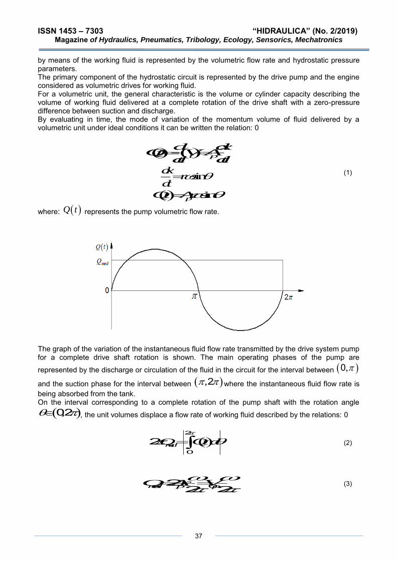
37
by means of the working fluid is represented by the volumetric flow rate and hydrostatic pressure parameters. The primary component of the hydrostatic circuit is represented by the drive pump and the engine considered as volumetric drives for working fluid. For a volumetric unit, the general characteristic is the volume or cylinder capacity describing the volume of working fluid delivered at a complete rotation of the drive shaft with a zero-pressure difference between suction and discharge. By evaluating in time, the mode of variation of the momentum volume of fluid delivered by a volumetric unit under ideal conditions it can be written the relation: 0
() ()t p
d dxQt VA
dt dt= =
sindx
rdt
=
() sinpQt Ar=
(1)
where: ( )Q t represents the pump volumetric flow rate.
The graph of the variation of the instantaneous fluid flow rate transmitted by the drive system pump for a complete drive shaft rotation is shown. The main operating phases of the pump are represented by the discharge or circulation of the fluid in the circuit for the interval between ( ),0and the suction phase for the interval between ( ), 2 where the instantaneous fluid flow rate is being absorbed from the tank. On the interval corresponding to a complete rotation of the pump shaft with the rotation angle ( ), 02 , the unit volumes displace a flow rate of working fluid described by the relations: 0
()medQ Qtd
=2
0
2 (2)
med p pQ Ar V
= =022 2
(3)

ISSN 1453 – 7303 “HIDRAULICA” (No. 2/2019) Magazine of Hydraulics, Pneumatics, Tribology, Ecology, Sensorics, Mechatronics
38
The relationship highlights the dependence between the theoretical average of fluid flow rates discharged by the drive pump with volume and the angular velocity at the pump shaft. The relation does not take into account the volume losses of the pump. From an energetic point of view, at a complete rotation of the pump shaft (P) the value of the
average energy ( )mE at the volumetric unit axis can be described by the relations: 0
dE pdV=
pdV Adx=
sindx r d=
sinpdEpAr d=
(4)
By integrating to a complete rotation of the pump shaft the medium energy relation to the pump shaft is obtained: 0
sinmed pE dEpAr d
= = 2
0 0
( )med p pE prAVp= =02
(5)
The ratio of average energy to the pump shaft reveals under theoretical conditions the proportional dependence between the value of the average energy and the pressure in the system, and the proportional factor is even the cylinder capacity of the pump. Extending elemental energy according to the required mean torque at the pump shaft, for a complete revolution of the pump shaft results: 0
meddE M d=
med medE M=2 (6)
The relation for the medium moment in theoretical value can be written at a complete rotation of the pump shaft as follows: 0
med pM Vp
= 012
(7)
The proportional dependence between the value of the mean moment at a complete rotation of the pump shaft and the pressure in the drive system, depending on the pump stroke and the value of the axis of rotation of the axle, can be observed. For an angular velocity in constant value ( )ct= the theoretical value of the mean power to the pump shaft is obtained: 00
med pM Vp = 012 (8)

ISSN 1453 – 7303 “HIDRAULICA” (No. 2/2019) Magazine of Hydraulics, Pneumatics, Tribology, Ecology, Sensorics, Mechatronics
39
med med medN M Qp= = (9)
The value of the required theoretical average power to the pump shaft is directly proportional to the value of the fluid pressure inside the actuation system and the proportionality factor is the value of the average flow rate of the pump in the working circuit.
3. Rotary lobe pump volumetric unit
Rotary lobe pumps belong to the group of rotating positive displacement pumps. Pump constructive solution is accomplished by arranging two lobe rotors inside a casing. The constructive particularity is ensured by the fact that the lobes have permanent contact with the housing or with the complementary rotor lobe. The working chambers that are necessary for the operation of the pump are delimitedin this manner. In order to synchronize the relative position of the two rotors and to precisely delineate the working chambers required for the two suction and discharge phases, toothed wheels are used. 0
Fig. 1. Lobe pump operation principle
The lobe pump present a compact design ad high performance in fluid circulation. These pump types are used to continuous convey and dose diferent fluids in relation with to special velocity values. Following rotor rotation, the fluid is captured from the suction area and sent to the discharge port through the space between the lobes and the housing. Circulation is provided along the walls of the casing and through the gear made between the two lobes a permanent seal is provided between the two low pressure pump zones and the high pressure zone corresponding to the pressure port area. The lobe pump has a compact design and high performance in fluid circulation. These pump types are used to continuously transport and deliver different fluids in relation to special rate values. The pump rotors motion causes a negative pressure at the suction orifice where the fluid is absorbed and circulated along the casing walls to the pressure orifice. The rotary lobe pumps are equally suitable for low and high-viscous fluid mediums. Due to their relative large spaces for fluid passage and low rotational velocity they are relatively tolerant to blockage due to solid particles within the circulated fluid. The lobe pump performance capacity is in higher value relative to many other positive displacement pumps of the same constructive type. At higher working pressure values over 80 bar these pump types present lower operating efficiency.

ISSN 1453 – 7303 “HIDRAULICA” (No. 2/2019) Magazine of Hydraulics, Pneumatics, Tribology, Ecology, Sensorics, Mechatronics
40
These pump types are generally used in auxiliary lubrication systems, but also for the transport and dosing of liquids. 4. Fluid flow aspects within lobe pump virtual model
In order to highlight certain operating aspects of the lobe pump volumetric unit, it is necessary to perform a fluid flow analysis on the virtual model of the lobe pump assembly. A three-dimensional assembly model was developed and introduced into the analysis made with the Ansys CFX program. The imported model is shown in the figure 2.
Fig. 2. Lobe pump functional model assembly
a) imported model b) mesh network of triangular elements
Fig. 3. Three-dimensional assembly model taken into consideration for flow analysis
The operating principle for this volumetric unit is based on the rotational motion of the two rotors which engage the fluid in motion along the casing wall. The pressure at the inlet it is at low values while for the outlet orifice is ensured the requisite pressure values. The flow rate values of liquid circulation are according with the volumetric capacity at a single rotation of pump shaft. The declared initial values for the liquid flow analysis within the lobe pump are as total pressure (stable) for the inlet port at 1 at and the axial motion of the lobes positioned inside the pump casing declared as immersed solid, material steel. The flow analysis main domains of the considered model are represented by the fluid region and the two lobes which are in continuous engagement keeping the permanent contact in the center of the fluid region thereby preventing the liquid leaking back towards the inlet region.

ISSN 1453 – 7303 “HIDRAULICA” (No. 2/2019) Magazine of Hydraulics, Pneumatics, Tribology, Ecology, Sensorics, Mechatronics
41
The mesh network was made with triangular shape elements, with 77293 nodes and 246811 elements. The working fluid is represented by mineral oil at 25 degrees Celsius with the shear stress transport turbulence option for the fluid region. The analysed fluid model has an inlet port for the working fluid and one outlet. According with the initial has been declared conditions of lobe rotational motion with a velocity of 11 rev/s. The liquid is taken from the inlet port and circulated along the outer walls to the outlet orifice. The results are presented in terms of pressure and fluid velocity values registered at the level of analysed fluid region (figure 4).
a) Fluid velocity values
b) Pressure values Fig. 4. The flow analysis obtained result values
Due to the lobes rotation it is observed on the results obtained the overall operation of the volumetric unit which is of sequential type of liquid transport according to the relative position of the driven rotors. A low pressure (depression) value is recorded for the fluid area corresponding to the fluid inlet or intake within the analyzed housing or fluid region, which is explicable for the external fluid pickup area through the intake port. As the fluid is shifted radially along the housing walls, higher pressure values are recorded up to the maximum values corresponding to the volume output region of the volumetric unit for each zone of the lobe that drives the liquid to the outlet. Velocity values are characteristic of the route followed by the liquid on the analyzed region and are obtained as a result of the specific rotation motion of the drive rotors. The diagrams for the pressure and velocity values recorded for the liquid flow analysis time steps on the analyzed model are shown in Table 1.
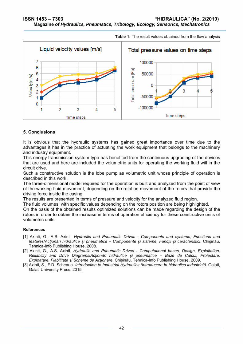
ISSN 1453 – 7303 “HIDRAULICA” (No. 2/2019) Magazine of Hydraulics, Pneumatics, Tribology, Ecology, Sensorics, Mechatronics
42
Table 1: The result values obtained from the flow analysis
5. Conclusions
It is obvious that the hydraulic systems has gained great importance over time due to the advantages it has in the practice of actuating the work equipment that belongs to the machinery and industry equipment. This energy transmission system type has benefited from the continuous upgrading of the devices that are used and here are included the volumetric units for operating the working fluid within the circuit drive. Such a constructive solution is the lobe pump as volumetric unit whose principle of operation is described in this work. The three-dimensional model required for the operation is built and analyzed from the point of view of the working fluid movement, depending on the rotation movement of the rotors that provide the driving force inside the casing. The results are presented in terms of pressure and velocity for the analyzed fluid region. The fluid volumes with specific values depending on the rotors position are being highlighted. On the basis of the obtained results optimized solutions can be made regarding the design of the rotors in order to obtain the increase in terms of operation efficiency for these constructive units of volumetric units.
References
[1] Axinti, G., A.S. Axinti. Hydraulic and Pneumatic Drives - Components and systems, Functions and features/Acţionări hidraulice şi pneumatice – Componente și sisteme, Funcții și caracteristici. Chişinău, Tehnica-Info Publishing House, 2008.
[2] Axinti, G., A.S. Axinti. Hydraulic and Pneumatic Drives - Computational bases, Design, Exploitation, Reliability and Drive Diagrams/Acţionări hidraulice şi pneumatice – Baze de Calcul, Proiectare, Exploatare, Fiabilitate și Scheme de Acționare. Chişinău, Tehnica-Info Publishing House, 2009.
[3] Axinti, S., F.D. Scheaua. Introduction to Industrial Hydraulics /Introducere în hidraulica industrială. Galati, Galati University Press, 2015.

ISSN 1453 – 7303 “HIDRAULICA” (No. 2/2019) Magazine of Hydraulics, Pneumatics, Tribology, Ecology, Sensorics, Mechatronics
43
Sensitivity Analysis of Sharp-Crested Weirs as a Function of Shape Opening, for Small Discharges
Assoc. Prof. Cristina Sorana IONESCU1, Assoc. Prof. Daniela Elena GOGOAŞE NISTORAN1, Assoc. Prof. Ioana OPRIŞ2, Assist. Ștefan-Mugur SIMIONESCU1
1 University Politehnica of Bucharest, Faculty of Power Engineering, Department of Hydraulics, Hydraulic Machines and Environmental Engineering, [email protected], [email protected] 2 University Politehnica of Bucharest, Faculty of Power Engineering, Department of Power Generation and Use
Abstract: The paper investigates the degree of measurement accuracy of several sharp – crested weirs of different shapes, based on the experimental results obtained in the laboratory. A sensitivity analysis is performed to assess the influence the weir shape has on the coefficients of discharge and to identify which one provides the best accuracy for measuring small discharges.
Keywords: Sharp-crested weir, coefficient of discharge, weir sensitivity, rectangular, triangular, trapezoidal, proportional weir.
1. Introduction
A weir consists of a vertical wall that blocks the flow, usually placed at the outlet of a tank, flume, channel or basin, being used for discharge measurement. Its basic operation principle is very simple: the liquid depth gradually increases till reaching the barrier height and then flows over its crest. The liquid level over the crest is a measure of the flow rate [1]. Weirs can be classified in accordance with several criteria (shape of the opening, shape of the crest, effect of sides on the nappe) [2], but one of the most common division is that of grouping them in sharp – crested and broad – crested weirs. The fundamental distinction between sharp and broad-crested weirs relates to the location of the critical depth that in facts controls the discharge [3]. Due to their accuracy [4], [5] sharp crested weirs have many practical applications, being widely used devices for low flow measurements in hydraulic laboratories as well as in situ for smaller rivers and canals [6]. Their main drawback in the field is that they frequently become clogged with debris or floating objects and must be periodically cleaned. Aydin et al. [5] showed that the most critical parameter defining the discharge accuracy measurement is the weir’s sensitivity, which is exclusively controlled by the head reading. The weir’s sensitivity is defined as the change of head per unit change of discharge, i.e., the 𝑑ℎ
𝑑𝑄 ratio or,
for a range discharge range Δ𝑄 as Δℎ
Δ𝑄. The higher this ratio, the weir is more sensitive, and the
accuracy of the flow estimate is higher. The notion of sensitivity is coupled with that of accuracy. The accuracy of the flow measurements provided by a weir depends not only on the accuracy of the calibration curve or of its corresponding formula, but also on the accuracy of the vernier height gauge scale and its readings. The reading error of this instrument, like any measurement operation, is subject to a certain absolute error, hence the occurrence of a flow measurement error. Usually, the quantity of concern is the relative discharge d𝑄
𝑄 error resulting from a 𝑑ℎ nappe height measurement error. As well,
other possible sources of errors are possible, such as those resulting from an inaccurate design or an inappropriate calibration of the weir. The resulting error d𝑄
𝑄 is a measure of the degree of
uncertainty associated with flow measurement [4], [7]. Stability of a weir implies having a constant discharge coefficient over the whole range of flow rates. The present paper investigates the sensitivity of 4 sharp – crested weir shapes (rectangular, triangular, trapezoidal and proportional), to assess which one provides the best accuracy for measuring small discharges.

ISSN 1453 – 7303 “HIDRAULICA” (No. 2/2019) Magazine of Hydraulics, Pneumatics, Tribology, Ecology, Sensorics, Mechatronics
44
2. Theoretical background
The head-discharge formula for a simple opening weir has the general form of a power law 𝑄 = 𝐾ℎ𝑛 = 𝐶𝑑𝑄𝑡 (1)
where Q is the actual flowrate, K is a dimensional coefficient, 𝐶𝑑- a non-dimensional discharge coefficient, 𝑄𝑡 the theoretical discharge and n - the exponent of the weir head. The exponent has different values pending on the weir’s shape (Fig.1). To take into consideration the influence of the liquid viscosity and surface tension a correction term ℎ𝑘 is added to provide an effective head, ℎ𝑒 = ℎ + ℎ𝑘 [4]. As well, to avoid drawdown errors, head must be measured at an upstream distance equal with 35 times its value [8].
Fig. 1. Sharp-crested weir opening shapes used in the study: a) rectangular; b) V-notch; c) trapezoidal; d) proportional (Sutro)
The non-dimensional coefficient of discharge, 𝐶𝑑 is a complex parameter, being triggered by a set of physical phenomena such as friction, surface tension, pressure distribution due to streamline curvature, nappe lateral contraction and vertical drawdown, velocity profile in the approach section and dependent on the weir geometry. For small heads, surface tension induces the clinging of the nappe to the weir and therefore a minimum head is required, to allow an accurate measurement. Depending on the weir geometry, equation (1) takes different forms.
p
h
B
b)
p
h
b
B
a)
p
h
b
2
B
c)
B
a
b
Datum
2/3
a
p
d)
h Hd
y
x(y
)

ISSN 1453 – 7303 “HIDRAULICA” (No. 2/2019) Magazine of Hydraulics, Pneumatics, Tribology, Ecology, Sensorics, Mechatronics
45
2.1 Rectangular weir Rectangular weirs (Fig.1.a) may be suppressed or contracted and are usually used in open channels, wastewater and sewage systems, being thus suited for relatively larger flowrates. To provide an accurate measurement it is recommended the head to be greater than 3 cm [8]. The relationship giving the flowrate of a rectangular weir with both side contractions is
𝑄𝑟 = 𝐶𝑑𝑟2
3√2𝑔(𝑏 − 0.2ℎ)ℎ3/2 (2)
where: 𝐶𝑑𝑟 is the non-dimensional discharge coefficient of the rectangular weir, b - the notch width and h - the head above the weir horizontal crest [9], [10] and g - the acceleration due to gravity. A variety of rectangular weir is the slit weir, having a narrow width, so that the 𝑏
𝐵 ratio of the weir
width over the channel width should not be greater than 0.17. Such weirs were used for measuring discharges smaller than 5 l/s in the laboratory [5]. 2.2 Triangular weir The triangular weir or V-notch sharp-crested weir (Fig.1.b) is a very useful tool for measuring small discharges in engineering fields such as hydraulics, environmental, chemical and irrigation [11]. Flow and head are related by the formula
𝑄𝑡𝑟 = 𝐶𝑑𝑡𝑟8
15√2𝑔𝑡𝑔 (
𝜃
2) ℎ5/2 (3)
where 𝐶𝑑𝑡𝑟 is the non-dimensional discharge coefficient of the V-notch weir and h the head over the weir vertex. A V-notch weir can measure relatively low flow rates and [4] reports its good precision and stability, i.e., errors smaller than 2%, provided both design conditions and recomended flow range for the weir are met, and water level measurements errors are kept under 1%. 2.3 Trapezoidal (Cipolletti) weir A trapezoidal weir integrates a rectangular weir with a triangular one (Fig.1.c) and therefore the discharge flowing over it is given by the addition of the relations (2) and (3):
𝑄𝑡𝑟𝑎𝑝. = 𝐶𝑑𝑡𝑟𝑎𝑝 (2
3√2𝑔𝑏ℎ
3
2 + 8
15√2𝑔𝑡𝑔
𝜃
2ℎ5/2) (4)
where 𝐶𝑑𝑡𝑟𝑎𝑝 is the non-dimensional discharge coefficient of the trapezoidal weir, θ/2 – angle between the weir side and vertical, h the head over the weir crest and b – the crest width. The trapezoidal weir is used for larger flowrates and for a given crest length, the discharge it provides is greater than the discharge provided by a rectangular weir having its width equal to the crest length. Cipoletti showed the weir with the angle between the side and the vertical of 14.28 has a minimum lateral contraction of the nappe, and therefore the shape became standardised [4]. Even though this type of weir is used for large flow rates, for the present study an unusual Cipoletti weir was designed with a very small bottom width to allow measurement of very low discharges. 2.4 Proportional weir (Sutro) The proportional sharp-crested weir is a type of weir providing a flow rate in direct proportion to the head, being used in a variety of engineering fields such as: sanitation, agriculture, environmental, chemical engineering, hydraulic [12-15]. Literature in the field presents several shapes of proportional weirs [14], [4], one of them being the Sutro weir (Fig. 1.d). The flowrate of the Sutro weir is given by the formula
𝑄𝑆 = 𝐾𝑆 (ℎ +2
3𝑎) = 𝐾𝑆𝐻𝑑 (5)
where h is the head over a rectangular base of height a above the weir crest, 𝐾𝑆 - a proportionality constant, 𝐾𝑆 = 𝐶𝑑𝑆𝑏√2𝑔𝑎, 𝐻𝑑 - the head over a datum, chosen at a/3 above the crest and 𝐶𝑑𝑆 the nondimensional coefficient of discharge. The shape of the weir curvilinear profile determined by Sutro has the form provided by the equation:

ISSN 1453 – 7303 “HIDRAULICA” (No. 2/2019) Magazine of Hydraulics, Pneumatics, Tribology, Ecology, Sensorics, Mechatronics
46
𝑥
𝑎= 1 −
2
𝜋𝑎𝑟𝑐𝑡𝑔√
𝑦
𝑎 (6)
A considerable advantage of the proportional weir when used at the downstream end of the grit chambers is that it maintains an almost constant velocity in these, which is very important in the process of gritt sedimentation for the varying sewage flows incoming at the wastewater treatment plants.
3. Experimental setup
The experimental setup consists in a hydraulic bench, equipped with a rectangular plexiglas flume (Fig.2.), four weirs of different shapes (rectangular, V-notch, trapezoidal and proportional-Sutro) were designed for a specified discharge range, built and used for measurements. Table 1 summarises the main geometrical and hydraulic features of the experimental setup. The rectangular and V-notch weir are made up of 3mm thick stainless steel plates with baveled downstream edge whereas the other two weirs were laser cut from 2 mm plexiglass plates using a numerically controlled machine. Water is recirculated through the hydraulic bench by means of a centrifugal pump and pipes. The discharge is measured by means of a calibrated diaphragm. The invert of the flume was maintained horizontal along the its length with the help of a bubble levelling indicator. The weir head was measured using a vernier height gauge level indicator having an accuracy of 0.2 mm, placed in a control section at a distance of 3-5 times the maximum head.
Fig. 2. Sketch of experimental setup
4. Method
To obtain reliable data, care was taken to allow flow to reach steady state conditions before each set of measurements, i.e. enough time for the flow to stabilise. Measurements were performed for increasing and decreasing flow rates between the maximum value delivered by the pump and minimum value for avoiding clinging nappe.
water supply tank
centrifugal pump
calibrated diaphragm
“U” differential manometer
Flume with weir

ISSN 1453 – 7303 “HIDRAULICA” (No. 2/2019) Magazine of Hydraulics, Pneumatics, Tribology, Ecology, Sensorics, Mechatronics
47
Table 1: Main geometric and hydraulic features of the experimental setup
Geometric and hydraulic feature
Rectangular V-notch Trapezoidal Proportional - Sutro
b (m) 0.03 - 0.01 0.04 b min. (m) - - - 0.0072
a (m) 0.005 - - - p (m) 0.065 0.065 0.065 0.065 () - 30 30 -
Qmin (l/s) 0.03 Qmax (l/s) 0.25
B (m) 0.135 Lflume (m) 0.8
H max. flume (m) 0.25
5. Results
In Fig. 3. are shown the head-discharge relationships for the studied weir shapes. One may observe that the Sutro weir dependence is close to a linear function, as expected for a proportional weir.
Fig. 3. Head-discharge relationships for the studied weir shapes
From Fig. 4. one may see that discharge coefficients show an increase with increasing flowrates for the case of trapezoidal weir, whereas for V-notch and rectangular weirs they decrease as flowrate increases. Discharge coefficients of the proportional weir practically remain constant. Higher and smaller than usual discharge coefficients are obtained for the cases of triangular and rectangular weirs respectively, possibly due to the fact that the prescribed minimum head requirement of 5 cm for the former and 2 cm for the latter [4] are not complied with for such small discharges measured in the laboratory.
0
10
20
30
40
50
60
0 0.00005 0.0001 0.00015 0.0002 0.00025
h(m
m)
Q(m3/s)
rectangular
triangular
trapezoidal
proportional

ISSN 1453 – 7303 “HIDRAULICA” (No. 2/2019) Magazine of Hydraulics, Pneumatics, Tribology, Ecology, Sensorics, Mechatronics
48
Fig. 4. Discharge coefficients for the studied weir shapes
Fig. 5. Approximated head-discharge relationships for the studied weir shapes
The experimental head-discharge curves were fitted (with very good correlation coefficients) with power functions (Fig. 5.) to identify the mean two parameters in equation (1): coefficient K and exponent n. For all studied weirs the resulted exponents are close to the corresponding theoretical values such as: 1.4311 (instead of 1.5), 2.3702 (instead of 2.5), 1.1445 (instead of 1) and 1.9793 (in the 1.5 and 2.5 range).
0.4
0.5
0.6
0.7
0.8
0 0.00005 0.0001 0.00015 0.0002 0.00025 0.0003
Cd
Q(m3/s)
Triangularrectangulartrapezoidalproportional
Q = 0.2956h2.3702
R² = 0.9998
Q = 0.0392h1.4311
R² = 0.9997
Q = 0.1633h1.9793
R² = 0.9997
Q= 0.0134h1.1445
R² = 0.9995
0.00001
0.0001
0.001
0.01 0.1
Q(m
3 /s)
h(m)
TriangularRectangularTrapezoidalProportional

ISSN 1453 – 7303 “HIDRAULICA” (No. 2/2019) Magazine of Hydraulics, Pneumatics, Tribology, Ecology, Sensorics, Mechatronics
49
Fig. 6. Sensitivity of the studied weirs as a function of head
Fig. 7. Sensitivity of the studied weirs as a function of discharge
Fig. 6 and Fig.7 present the sensitivity of the studied weirs as a function of head and discharge, respectively. For heads smaller than 4.5 cm the best sensitivity belongs to the V notch, but the proportional weir becomes the most sensitive for heads greater than this value. As well, the triangular weir has the highest sensitivity for discharges smaller than about 0.152 l/s, whereas for greater values of flowrates the proportional weir takes the lead. For heads lower than 2.5 cm and flowrates smaller than 0.11 l/s, the second-best sensitivity belongs to the trapezoidal weir. Results also show a surprisingly better sensitivity of the rectangular weir, as compared with the proportional weir, for heads smaller than 1 cm and discharge values under 0.068 l/s. This could be attributed to the fact that accurate measurements for the rectangular weir can be made only for heads greater than 2 cm [4], However, when computing the relative discharge d𝑄
𝑄 error resulting
40
400
4000
0 0.01 0.02 0.03 0.04 0.05 0.06
dh
/dQ
h (m)
rectangulartriangulartrapezoidalproportional
5.E+01
5.E+02
1.E-05 1.E-04
dh
/dQ
Q (m3/s)
rectangular
triangular
trapezoidal
proportional

ISSN 1453 – 7303 “HIDRAULICA” (No. 2/2019) Magazine of Hydraulics, Pneumatics, Tribology, Ecology, Sensorics, Mechatronics
50
from a 𝑑ℎ = 0.2 mm nappe height measurement error, one can see that the highest degree of uncertainty associated with flow measurement lies with the V notch, whereas the proportional weir has the best accuracy for all head ranges (relative discharge errors under 2%).
Fig. 8. Relative error of the measured discharge for 0.5 mm error of measured head
as a function of head
6. Conclusions
The superiority of the Sutro weir over the non-linear weirs such as the rectangular, triangular and trapezoidal weirs is obvious in terms of multiplication of the head reding errors into the discharge ones. The former induces practically an equal error in discharge, whereas the V notch, rectangular and trapezoidal weirs induce errors of 1.42, 2.37 and 1.97 times into the discharge values respectively. For flowrates smaller than 0.152 l/s the best sensitivity among the studied weirs belongs to the V-notch. Above this value, in the studied discharge range, the proportional weir has the best sensitivity. Therefore, these two opening-shapes of sharp-crested weirs proved to be the best for applications of measuring very low discharges.
References
[1] Bengtson, H.H. ”Sharp-Crested Weirs for Open Channel Flow Measurement”, Course #506, 2011, Accessed May 4, 2019. https://docplayer.net/21027275-Sharp-crested-weirs-for-open-channel-flow-measurement-course-506-presented-by.html.
[2] Bansak, R.K. A textbook of Fluid Mechanics and Hydraulic Machines. Revised 9th Edition. New Delhi: LAXMI Publications, 2010.
[3] Sutherland, E., and T. Taylor. “Weirs”, CIVE 401 – Hydraulic Engineering, 2014, Accessed May 4, 2019. https://www.engr.colostate.edu/~pierre/ce_old/classes/CIVE%20401/Team%20reports/13%20-%20Sharp%20and%20Broad-crested%20Weirs%20-%20Sutherland%20Taylor.pdf.
[4] Bos, M.G. (ed.) Discharge measurement structures. Revised 3rd Edition. International Institute for Land Reclamation and Improvement/ILRI, Wageningen, The Netherlands, 1989.
[5] Aydin, I., M.A. Ger, and O. Hincal. “Measurement of Small Discharges in Open Channels by Slit Weir.” Journal of Hydraulic Engineering 128, no. 2 (February 2002): 234-237.
[6] Claydon, J.F. “Sharp- crested weir 2”, Accessed April 10, 2019. http://www.jfccivilengineer.com/ sharp_crested_weir_2.htm.
0.00%
1.00%
2.00%
3.00%
4.00%
5.00%
6.00%
7.00%
8.00%
9.00%
10.00%
0 0.01 0.02 0.03 0.04 0.05 0.06
dQ
/Q
h (m)
Rectangular
Triangular
Trapezoidal
Proportional
Lower limit of h
Upper limit of h

ISSN 1453 – 7303 “HIDRAULICA” (No. 2/2019) Magazine of Hydraulics, Pneumatics, Tribology, Ecology, Sensorics, Mechatronics
51
[7] Beaudry, J.-P., and J.-C. Rolland. Mécanique des fluides appliquée. 2e édition revue et corrigée. Québec, 2005.
[8] American Society for Testing and Materials, ASTM D-5242-92 (2013). “Standard Test Method for Open Channel Flow Measurement of Water with Thin-Plate Weirs.” ASTM International, West Conshohocken, PA, 2013.
[9] Kindsvater, C.E., and R.W.C. Carter. “Discharge characteristics of rectangular thin plate weirs.” Journal of Hydraulic Division. ASCE 83, no. 6 (1957): 1-36.
[10] King, H.W., C.O. Wisler, and J.G. Woodburn. Hydraulics. 5th Editon. London, John Wiley and Sons, 1995.
[11] Ali, M.S., A. Qadri, and T. Mansoor. “Flow characteristics of a triangular sharp crested weir.” Paper presented at the HYDRO 2015 International Conference, Roorkee, India, December 17-19, 2015.
[12] Stout, O.V.P. “The proportional flow weir devised in 1896.” Engineering News 72, no. 9 (1914): 148-149. [13] Pratt, E.A. “Another proportional-flow weir: Sutro weir.” Engineering News 72, no. 9 (1914): 462-463. [14] Keshava Murthy, K. “The theory of proportional weirs.” J. Indian Inst. Sci. 75 (July-Aug. 1995): 355-372. [15] Keshava Murthy, K., and N. Seshagiri. “A generalized mathematical theory and experimental verification
of proportional notches.” J. of the Franklin Institute 285, no. 5 (May 1968): 347-363.

ISSN 1453 – 7303 “HIDRAULICA” (No. 2/2019) Magazine of Hydraulics, Pneumatics, Tribology, Ecology, Sensorics, Mechatronics
52
From Human-Environment Interaction to Environmental Informatics (IV): Filling the Environmental Science gaps with Big Open-Access Data
Assoc. Prof. eng. Mirela COMAN1, PhD stud. Bogdan CIORUȚA2
1 Technical University of Cluj-Napoca - North University Centre of Baia Mare, Faculty of Engineering, str. Victor Babeș 62A, 430083, Baia Mare; [email protected]
2 Technical University of Cluj-Napoca - North University Centre of Baia Mare, Office of Information and Communication, str. Victor Babeș 62A, 430083, Baia Mare; [email protected]
Abstract: Nowadays, environmental data lifecycle management becomes more and more important in the context of local and regional communities sustainable development strategies. Enormous volume of environmental data is generated by an increasing number of devices across the world; correct and efficient surveillance of environment throughout data lifecycle management is essential for optimisation of the utility of those data pieces and minimisation of error potential. Starting from the idea of sustainable development in accordance to the latest sustainability diagram framework, using the tools provided by the Environmental Informatics Systems, we propose to show that, on the Human-Environment Interaction - Environment Informatics circuit, whatever the environment offers as primary data and what we offer back to the environment needs to represent the real state in the field, with which the environment copes. On the validity and viability of the respective situation depends, after all, our common future, based on harmony between society-economy-environment.
Keywords: Human-Environment Interaction, environmental big data, data acquisition, Knowledge Society.
1. Introduction
Nowadays, the era that we live can be described as the “Information Age”, sometimes even as the “Knowledge Age”. No matter what area of science and technology we look at, it is obvious that we are dealing with an ‘information overflow’ without precedent in the history of mankind [1, 2]. In this context, Environmental Sciences are no exception and recent advances in this field, also considering environmental monitoring and protection activities, would have been unthinkable, unmanageable and unattainable without the support offered by modern information technology [1], in the sense of Environment Information Systems (EISs) and Environment Informatics (EI) [4, 5], as part of the Sustainable Informatics (SI).
Fig. 1. Knowledge Society as a mixture between knowledge and sustainability index [2]
In its turn, Sustainable Informatics (SI) via sustainability index is integrated in Knowledge Society (as in Fig. 1) [3], where it play an important role, for environmental data-dependent actors, in decision-making [4, 5], problem solving, analyzing trends [6-8], understanding their customers, and doing research, being closely linked with environmental requirements in decades [9, 10].

ISSN 1453 – 7303 “HIDRAULICA” (No. 2/2019) Magazine of Hydraulics, Pneumatics, Tribology, Ecology, Sensorics, Mechatronics
53
2. From Environment Surveillance and Monitoring to Environmental Big Data evolution
More often than ever, we are talking about the “information explosion” or “information abundance”, suggesting in fact through these expressions the existence of a huge data and/or information volume and, at the same time, the difficulty in accessing, selecting and evaluating the information resources [11]. In this sense, it is appreciated that the feeling of being overwhelmed by data and/or information is due to the inability to extract from a huge volume of data - big data (see a concept representation in Fig. 2) or information resources the really relevant elements.
Fig. 2. A mind-map example for the Big Data concept
The great problem of information remains the vast amount of data resources that are unaware of limitations under any form of society's activity. In order to have an image of the informational dimension of society as a whole, we must not overlook the fact that “flooded with techniques, some scientists complain that instead of experimenting, they lose more time trying to see whether was not done before someone else” [11]. In such context, it is extremely difficult to identify information items, especially those that are really important. 2.1 Environment surveillance and monitoring Likewise, environment observations, as primitive forms of information about a change, tendency or development in industrial, economical, national or global environments, are key pieces of data, which together contribute to building and improving the understanding of interactive processes in the Earth's environment or reality and developing a more coherent image (as suggested in Fig. 3) of its sensitivities towards natural and human-induced changes.
Fig. 3. The reality-observation-knowledge triangle as a primitive representation for environment surveillance

ISSN 1453 – 7303 “HIDRAULICA” (No. 2/2019) Magazine of Hydraulics, Pneumatics, Tribology, Ecology, Sensorics, Mechatronics
54
Modern environment surveillance and monitoring systems in collaboration with policies, strategies and governmental actions - transposed to national, regional and local levels, provide evidence regarding causes, tendencies and consequences of ecosystem changes on different scales. As reflected by Fig. 4, there are four steps in connection with modern environment surveillance and monitoring, as follows: data acquisition and aggregation (step 1), data processing, machine learning and pattern recognition (step 2), geospatial analytics and insights (step 3), and, last but not least, online decision support and data science (step 4).
Fig. 4. Different aspects of the environment surveillance and monitoring
Environmental observations, since “the environment” gained its place in the public international agenda, have already been used to reduce the impact of natural hazards, which can have a really significant cost per year, and have the potential to also improve other areas like business analytics, agricultural production and urban planning, the sustainable development of the community [12-14]. In order to support the green economy, with highly accurate environmental data, by creating flexible long-term environmental surveillance systems, is more than just natural and necessary to consider the SI exploring approaches to measurement, analysis, up- and down-scaling and modeling of whole ecosystems. This aspect will guarantee that we, as a community with responsibility towards the environment, can easily detect, and interpret change and help decision-makers assess policy and resource management options by quantifying environmental and socio-economic impacts, via systematic and unsystematic environmental observations (see Table 1).
Table 1. Types of systematic and unsystematic environmental observations (adapted after [15-18])
Systematic environmental observations
vs. Unsystematic environmental observations
Scientific or unscientific methods of environmental observation
direct vs. indirect measurement taken in relation to behavior measured global vs. specific variety of behavior observed by researcher
noticed vs. unnoticed participant awareness obtrusive vs. non-obtrusive influence on participants or environment
participant vs. non-participant involvement with participants reactive vs. non-reactive participant reaction
structured observation vs. unstructured
observation with or without observation checklists
qualitative vs. quantitative - naturalistic vs. laboratory -
human vs. non-human human (classic) observations will be replace with non-human (innovative) observations of environment quality

ISSN 1453 – 7303 “HIDRAULICA” (No. 2/2019) Magazine of Hydraulics, Pneumatics, Tribology, Ecology, Sensorics, Mechatronics
55
According to the Table 1, an environmental observation can be sometimes casual in nature or sometimes it may act scientifically; an observation with a casual approach involves observing the right thing at the right place and also at the right time by a matter of chance or by luck, whereas a scientific observation involves the use of the tools of the measurement. A very important point to be kept in mind here is that all the environmental observations are not scientific in nature. Natural observation involves observing the behavior in a normal setting, no efforts are made to bring any type of change in the behavior of the observed; improvement in the collection of information and improvement in the environment of making an observation can be done with the help of non-natural observations (laboratory, by excellence). With the help of the direct method of observation, the observer is physically present; indirect method of observation involves studies of the different data recordings or information formats about the state of the environment, as in Fig. 5.
Fig. 5. Different publication formats for environmental data or information
At a closer look to common formats for environmental data and/or information, we could mention that the Knowledge Society manifest significant interest in:
• books - usually a substantial amount of information, published at one time and requiring great effort on the part of the author and a publisher;
• magazines or journals - published frequently, containing lots of articles related to some general or specific professional research interest;
• newspapers - each is a daily publication of events of social, political and lifestyle interest; • web sites - digital items, each consisting of multiple pages produced by someone with
technical skills or the ability to pay someone with technical skills; • articles - distinct, short, written pieces that might contain photos and are generally timely; • conference papers - written form of papers delivered at a professional or research-related
conference. Authors are generally practicing professionals or scholars in the field; • blogs - frequently updated websites that do not necessarily require extensive technical
skills and can be published by virtually anyone for no cost to themselves other than the time they devote to content creation. Usually marked by postings that indicate the date when each was written, and documentaries - works, such as a film or television program, presenting political, social, or historical subject matter in a factual and informative manner and often consisting of actual news films or interviews accompanied by narration;
• online videos - short videos produced by anybody, with a lot of money or a little money, about anything for the world to see, and podcasts - digital audio files, produced by anyone and about anything, that are available for downloading, often by subscription.
Structured environmental observation works according to a plan, involves specific information of the units that are to be observed and also about the data that is to be recorded - the operations that are to be observed and the various features that are to be noted or recorded are decided well in advance; in the case of the unstructured environmental observation, its basics are diametrically

ISSN 1453 – 7303 “HIDRAULICA” (No. 2/2019) Magazine of Hydraulics, Pneumatics, Tribology, Ecology, Sensorics, Mechatronics
56
against the structured environmental observation - the observer has the freedom to note down what he/she feels is correct and relevant to the point of study and also this approach of observation is very suitable in the case of exploratory research. Controlled environmental observations are the observations made under the influence of some of the external forces and such observations rarely lead to improvement in the precision of the research results. Non-controlled environmental observations are made in the natural environment, and reverse to the controlled observation these observations involve no influence or guidance of any type of external force. Observations made while using the scientific method can be quantitative or qualitative; observations are quantitative if they return numerical data, and qualitative research is when observations are recorded without capturing numeric data values - this type of observation is more subjective and relies on the researcher's interpretations. 2.2 Defining the Environmental Big Data Big Data was the buzz phrase of the recent years, but in truth, the concept has been around far longer than that; we know what data is - it is the raw information collected from any study, but particularly in sciences, so we expose some dictionary definitions, as follows [19, 20]:
• environmental data means any measurements or information that describe environmental processes, location or conditions, ecological or health effects and consequences, or the performance of environmental technology;
• environmental data include information collected directly from measurements, produced from models and compiled from other sources such as databases or literature;
• environmental data means any parameters or pieces of information collected or produced from measurements, analyses, or models of environmental processes, conditions, and effects of pollutants on human health and the environment, including results from laboratory analyses or from experimental systems representing such processes and conditions.
Environmental Big Data takes environmental data concept one step further - it is an environmental data set of such complexity that it would be impossible to select, preprocess, examine, manipulate, present and evaluate, as in Fig. 6, using traditional and dedicated methods. The intended results are often so complex that it's difficult to process even using tried and tested methods. It's important to note that the term does not necessarily denote the size of the data set (although a large volume of data is unavoidable), merely its complexity.
Fig. 6. An example of environmental data transformation process
Environmental Big Data is a term that describes the large volume of data - both structured and unstructured - that inundates a domain of interest or area of activity on a day-to-day basis, but it’s not the amount of data that’s important, it’s what community do with the data that matters. Environmental Big Data can be analyzed for insights that lead to better decisions and strategic eco-friendly moves in the context of a social-ecological system (SES), from 3 Vs models up to 15 Vs models, having the main 10 characteristics exposed in Fig. 7.

ISSN 1453 – 7303 “HIDRAULICA” (No. 2/2019) Magazine of Hydraulics, Pneumatics, Tribology, Ecology, Sensorics, Mechatronics
57
In actual context, the environmental data lifecycle is the sequence of stages that a particular unit of data goes through from its initial generation (or acquisition) to its eventual archival and/or deletion at the end of its useful life, or information dissemination [17].
Fig. 7. The 10 main characteristics of Environmental Big Open-Access Data Vs models
Although specifics vary, data management experts often identify five or more stages in the data life cycle. Once we know what data we are looking for, we should follow the next steps [17]:
• data acquisition refers to data collection from different sources; • data pre-processing refers to data transformation from streams of bytes into the proper
formats that will have a meaning to Big Data tools and technologies; • data clean up is a critical step, though in many occasions it is forgotten or carried out
leniently, the gross data acquired in the first phase may include bias, may have Data Deserts and/or may be subjected to Data Mirage effects, but during data clean up, we create a new data set that represents a better image of we are interested in analyzing;
• data analysis is the following step. Once we have the data in the appropriate format and structure and cleaned up, we start asking questions such as: Do we see any trend? Is there any kind of consolidated information this data shows? Can we infer some patterns?
• data visualization, sometimes carried out in parallel with data visualization, there are a great number and variety of data visualization tools.
• data interpretation. Together with the Data Clean up step in the Big Data processing cycle, this is also a critical step. There are many instances in which Data Interpretation has not been carried out adequately, leading to the wrong conclusions.
• data intervention. Once the conclusions have been achieved, this will lead to the next step which may involve using the data to take decisions, train Machine Learning algorithms, or rethinking the data gathering for the future.
In the scientific literature there are a few Vs models for Environmental Big Open-Access Data that integrate the following aspects:
• 3 Vs of Environmental Big Open-Access Data (volume - data galore, is self-explanatory; variety - complexity, types and formats; and velocity - actual speed of data);
• 4 Vs of Environmental Big Open-Access Data (3 Vs + veracity - uncertain or imprecise data; or 3 Vs + value - characterizing the potential of data to transform plans in actions);
• 5 Vs of Environmental Big Open-Access Data (4 Vs + visualization or 4 Vs + value); • 6 Vs of Environmental Big Open-Access Data (5 Vs + variability - this refers to dynamic,
evolving data, time series, seasonal, and any other type of non-static behavior in data sources; or 5 Vs + validity - clean data);
• 7 Vs of Environmental Big Open-Access Data (volume, variety, velocity, veracity, value, visualization, variability);
• 8 Vs of Environmental Big Open-Access Data (volume, variety, velocity, veracity, value, visualization, viscosity, virality);
• 9 Vs of Environmental Big Open-Access Data (8 Vs + venue - where the data comes from, multiple platforms; or 8 Vs + vocabulary - semantics and other context-based metadata that describe the data‘s structure, syntax, content and provenance);
• 10 Vs of Environmental Big Open-Access Data (9 Vs + vagueness - confusion over the meaning of big data);
• 11 Vs of Environmental Big Open-Access Data (10 Vs + volatility);

ISSN 1453 – 7303 “HIDRAULICA” (No. 2/2019) Magazine of Hydraulics, Pneumatics, Tribology, Ecology, Sensorics, Mechatronics
58
• 12 ... 14 Vs of Environmental Big Open-Access Data (different combinations of Vs); • 15 Vs of Environmental Big Open-Access Data (volume, variety, velocity, veracity, value,
variability, viability, visualization, virality, viscosity, volatility, validity, vocabulary, venue and vagueness).
Environmental Big Open-Access Data model/concept-diagram is determined using a few metrics, closely related to the number of parameters, starting with the simplest approach - 3 Vs (as presented in Fig. 8) and ending with the most recent - with no less than 15 parameters.
a) b) c)
Fig. 8. Examples of the 3 Vs Environmental Big Open-Access Data models a) detailed hexagonal model; b) detailed target distributed model; c) detailed segmented cycle model.
In the same context, to be relevant, Environmental Big Open-Access Data must be able to cope with the speed at which data is generated in order to store it and retain the most up-to-date and relevant information. This is useful in most areas related to environment protection, but vital in early warning systems ahead of natural disasters or to detect inappropriate activities which interferes with the environmental protection. The fourth dimension of Environmental Big Open-Access Data is veracity - handling data in doubt (see a few 4 Vs models in Fig. 9).
a) b) c)
d) e)
Fig. 9. Examples of the 4 Vs Environmental Big Open-Access Data models a) basic segmented cycle model; b) basic segmented square model; c) detailed segmented square model;
d) V-shaped detailed block model; e) O-shaped detailed quadrant model.

ISSN 1453 – 7303 “HIDRAULICA” (No. 2/2019) Magazine of Hydraulics, Pneumatics, Tribology, Ecology, Sensorics, Mechatronics
59
Arguably the most important, but surprisingly a new addition, from 4 to 5 Vs models, in environmental sciences, is the need for verifiable environmental data - veracity, uncertainly of environmental data (see Fig. 10).
a) b)
Fig. 10. Examples of the Environmental Big Open-Access Data models with 5 parameters a) basic segmented cycle model; b) detailed cycle matrix model
In order to determine a data set's accuracy and integrity, not just of the data, but also the sources that generate it, we need to underline the connection between Big Data and Open-Data models, as in Fig. 11; if there is no trust in the environmental data source, the data itself is virtually useless.
a) b)
c)
Fig. 11. Examples of the Environmental Big Open-Access Data models with 6 parameters a) detailed block list model; b) detailed hexagonal-block model;
c) the integration between Big Data and Open-Data models

ISSN 1453 – 7303 “HIDRAULICA” (No. 2/2019) Magazine of Hydraulics, Pneumatics, Tribology, Ecology, Sensorics, Mechatronics
60
The complexity of Environmental Big Open-Access Data models with more than 6 parameters is defined, in the development-context of EISs and EI, as any data that cannot be captured, managed and/or processed using traditional data management components and techniques. To express this kind of complexity we refer to it in Fig. 12.
a)
b) c)
Fig. 12. The ecomplexity of the Environmental Big Open-Access Data models a) detailed block list model; b) detailed multi-triangle-block model; c) the graph/network model
3. Conclusions
Environmental data lifecycle management is becoming increasingly important, especially in the context of the attempts of sustainable development of communities, and since the explosion of environmental big data and the ongoing development of the Internet of Things (IoT). Enormous volumes of environmental data or environmental big open-access data are being generated by an ever-increasing number of devices all over the world. Proper oversight of this data throughout its lifecycle is essential to optimize the decision-making, problem solving, analyzing trends and so on, to generate a better future for the next generations.

ISSN 1453 – 7303 “HIDRAULICA” (No. 2/2019) Magazine of Hydraulics, Pneumatics, Tribology, Ecology, Sensorics, Mechatronics
61
References [1] Cioruţa, B., M. Coman, and A. Cioruţa. (2012) “GeoGebra software – a new possibility for studying the
environmental problematics?” Journal of Environmental Research and Protection (Ecoterra®), no. 30: 40-47, www.ecoterra-online.ro/files/1339069750.pdf.
[2] ***. https://blog.epa.gov/2016/10/21/filling-the-gaps-in-environmental-science-with-big-data. [3] Afgan, N.H., and M. Carvalho. ”The Knowledge Society: A Sustainability Paradigm.” Cadmus Journal® 1,
no. 1 (2010): 28-41, www.cadmusjournal.org/.../The Knowledge Society A Sustainability Paradigm.pdf. [4] Cioruţa, B., and M. Coman. “The evolution, definition and role of Environmental Information Systems in
the development of environmental protection strategies”/”Evoluţia, definiţia şi rolul SIM în dezvoltarea strategiilor pentru protecţia mediului.” Journal of Environmental Research and Protection (Ecoterra®, no. 27 (2011): 11-14, www.ecoterra-online.ro/files/1321371401.pdf.
[5] Cioruţa, B., and M. Coman. “A forey in modern scientific research of the environment. From EISs to EI”/”Incursiune în cercetarea ştiinţifică modernă a mediului înconjurător. De la Sistemele Informatice de Mediu la Informatica Mediului.” Journal of Environmental Research and Protection (Ecoterra®), no. 29 (2011): 17-20, www.ecoterra-online.ro/files/1330955124.pdf.
[6] Avouris, N.M., and B. Page. Environmental Informatics: Methodology and Applications of Environmental Information Processing. Dordrecht, Boston, Kluwer Academic, 1995.
[7] Günter, O. Environmental Information Systems. Berlin, Springer, 1998. [8] Hilty, L.M., B. Page, F.J. Radermacher, and W.F. Riekert. Environmental Informatics as a new Discipline
of Applied Computer Science. In Avouris, N., and B. Page, (Eds.). Environmental Informatics – Methodology and Applications of Environmental Information Processing. Dordrecht, 1995.
[9] Page, B., and L.M. Hilty. Trends in Environmental Information Processing. In Brunnstein, K., and E. Raubold (Eds.). Applications and Impacts. IFIP Transactions A-52. Amsterdam, 1995.
[10] Page, B. Environmental Informatics - Towards a new Discipline in Applied Computer Science for Environmental Protection and Research. In: Denzer, R., G. Schimak, and D. Russel (Eds). Environmental Software Systems. Proceedings of the International Symposium on Environmental Software Systems, May 1996, Pennsylvania State University, Malvern, London.
[11] Cioruţa, B., A. Cioruţa, and M. Coman. “Pleading for an environmental informatic culture forming need (Pledoarie pentru necesitatea formării unei culturi informaţionale environmentale.” Journal of Environmental Research and Protection (Ecoterra®), no. 30 (2012): 31-39, www.ecoterra-online.ro/files/1339069625.pdf.
[12] Cioruța, B., and M. Coman. “Environmental Informatics - solutions and emerging challenges in environmental protection.”, Studia Universitatis Babeș-Bolyai AMBIENTUM 57, no. 2: 17-30. Paper presented at International Conference „Environmental Legislation, Safety Engineering and Disaster Management”(ELSEDIMA®), Oct. 25-27 2012, Cluj-Napoca http://studia.ubbcluj.ro/download/pdf/903.pdf.
[13] Cioruţa, B., M. Coman, and V. Mateșan. “Environmental Information Systems: solutions and emerging challenges for modern strategic development of Romanian local communities.” Paper presented at International Conference "Scientific Research and Education in the Air Force" (AFASES®), May 23-25, 2013, Braşov, www.afahc.ro/.../Cioruta_Coman_Matesan.pdf.
[14] Cioruța, B., M. Coman, A.A. Cioruța, and A Lauran. “From Human-Environment Interaction to Environmental Informatics (I): Theoretical and Practical Implications of Knowledge-based Computing.” Magazine of Hydraulics, Pneumatics, Tribology, Ecology, Sensorics, Mechatronics (Hidraulica®) no. 1 (March 2018): 71-82, hidraulica.fluidas.ro/2018/nr1/71-82.pdf.
[15] ***. https://digitalfullpotential.com/big-data-processing-cycle-pitfalls. [16] ***. www.mbaofficial.com/mba-courses/research-methodology/what-are-the-types-of-observation. [17] ***. http://analytics.rsystems.com/data-engineering. [18] ***. https://peda.net/kenya/ass/subjects2/computer-studies/form-3/data-processing/dpc2. [19] ***. www.chesapeakebay.net/discover/glossary#E. [20] ***. www.popstoolkit.com/_glossary.aspx?l=E.

ISSN 1453 – 7303 “HIDRAULICA” (No. 2/2019) Magazine of Hydraulics, Pneumatics, Tribology, Ecology, Sensorics, Mechatronics
62
Equipment for Obtaining Thermal Energy by Using Biomass
Ph.D. Eng. Gabriela MATACHE1, Ph.D. Student Ioan PAVEL1, Ph.D. Eng Gheorghe ȘOVĂIALĂ1, Dipl. Eng. Alina Iolanda POPESCU1,
Ph.D. Student Eng. Mihai-Alexandru HRISTEA1
1 Hydraulics and Pneumatics Research Institute INOE 2000-IHP, [email protected]
Abstract: This paper presents the results obtained from testing a TLUD-type equipment, used to obtain biogas and biochar from biomass, developed and manufactured based on a patent elaborated under a research and development project by the staff of the Institute IHP. The paper presents solutions to increase the energy efficiency of burning boilers with gasification by recovering heat from the exhaust gases (which otherwise would be lost to the atmosphere) and reinserting it into the air circuit for gasification or combustion. The energy thus reintroduced into the combustion process can increase efficiency of gasification boilers by several percent, which means it saves large amounts of biomass and slows down global warming.
Keywords: Biomass, Combustion Processes, Gasifier, Thermal Energy, TLUD
1. Introduction
An imperative of our times is the development and use of green and economic technologies in clean energy production, in a sufficient high amount. The clean attribute refers specifically to the minimal impact that the energy production technology should have with the environment. The use of renewable energies is a characteristic of contemporary society, which is facing the decrease of classical resources, the rise in fuel prices and the pollution generated by their burning. However, the use of renewable resources to provide energy needs is still far from its full potential; this is also because of the lack of efficient conversion tools able to exploit various resources in mono-source or combined energy systems [1]. Increased efficiency in combustion processes is a goal proposed in all strategies of research and innovation, energy or environment. In the process of gasification, the inputs are biomass and air, while the outputs are fuel gas, biochar and ash, with a negative balance of carbon emissions due to carbon sequestration by biochar. The TLUD gasification principle (Figure 1) occurs when the biomass layer is introduced into a reactor and rests on a grid through which the air flow for gasification circulates from bottom to top. Gasification boilers operate under nominal conditions to maintain the temperature on the chimney at approx. 200° C to avoid condensation phenomenon (the formation of tar deposits).
2. General principles of biomass gasification
Priming gasification process is done by igniting the top layer of the biomass in the reactor. The combustion front descends continuously by consuming the biomass in the reactor. Due to the heat radiated from the oxidation front the biomass is heated, dried, and then it enters a fast pyrolysis process that releases volatiles and there remains unconverted carbon. By the time the combustion front reaches the grill all the volatiles in the biomass were gasified and some of the fixed carbon was reduced; about 10 - 20% of the initial mass remained on the grill, in the form of sterile “green charcoal”, called biochar. The proportion of biochar, in which most of the ash from biomass is incorporated, depends both on the carbon stored in the biomass and on the temperature maintained in the carbon reduction reaction; a high temperature ensures the reduction of more carbon. If the supply with gasification air continues, we switch to an updraft gasification process in which a layer of incandescent charcoal is kept on the grill; of this, there results mainly CO and little CO2, which passing through the hot charcoal layer enters the reduction reaction C+CO2 2CO. This second phase is called charcoal gasification.

ISSN 1453 – 7303 “HIDRAULICA” (No. 2/2019) Magazine of Hydraulics, Pneumatics, Tribology, Ecology, Sensorics, Mechatronics
63
Compared to direct combustion or gasification processes of wood and pellets, the TLUD gasification process is characterized by very low values of the superficial gas velocity through the oxidation front, resulting in a very low content of atmospheric particulate matter (PM), PM < 5 mg/MJ, well below the required standard in the EU since 2015 for biomass combustion processes, which is 25 mg/MJ. The gasification process is done with a reduced intensity with a specific hourly consumption of biomass of 80 – 150 kg/m2h, which leads to reduced specific powers of 250 – 350 kW/m2 of the reactor. The slow process maintains the superficial speed of the generator gas produced at very low values, vsup ≤ 0.06 m/s, which ensures reduced traction of free ash, and also at concentrations of PM2.5 of maximum 5 mg/MJbm when leaving the burner; this value is at least five times lower than current standards required for solid fuel heat generators. [3, 4, 5, 6, 7] The stages of the gasification process take place simultaneously in different areas of the reactor. These stages are: drying, pyrolysis, oxidation and reduction. Drying is necessary because the moisture content of the biomass is variable, ranging from 5 to 55%. At temperatures above 100° C, the water is removed and turned into steam. During the drying process, the biomass does not suffer any decomposition. Pyrolysis takes place in the temperature range of 150 - 700° C, and it consists of thermal decomposition of biomass in the absence of oxygen. Oxidation takes place by the aid of the air introduced into the oxidation zone. The air contains, together with oxygen, water vapor, inert gases, nitrogen and argon that do not react with the biomass components. Oxidation takes place at 700-2000° C. Reduction occurs in the reduction zone of the reactor. Here several chemical reactions take place at a temperature of 800 - 1000° C and in the absence of oxygen. The generator gas is a mixture of combustible and non-combustible gases. The combustible gases are: carbon monoxide (15 - 30%), hydrogen (10 - 20%), methane (2 - 4%). The non-combustible gases are: nitrogen (45 - 60%), water vapors (6 - 8%), carbon dioxide (5 - 15%) [8]. The fuel gas can be used for:
- burning in a specialized burner, resulting in high enthalpy combustion gases which contain very low concentrations of mechanical particles (MP) and CO, hot gases which are used in:
- the process of heating water, steam or air, - external combustion engines to produce electric power
After filtering off the tar and MP contents, the fuel gas can be used in internal combustion engines to produce electric power. Figure 1 is a block diagram of the procedure of energy recovery of biomass by thermo-chemical gasification.
Fig. 1. The block diagram of energy recovery of biomass by gasification MP mechanical particles; e.c.e. external combustion engine; i.c.e. internal combustion engine
3. Biomass gasification procedures
Two types of gasification procedures are currently being used: up-draft (counter-current) and down-draft (co-current).

ISSN 1453 – 7303 “HIDRAULICA” (No. 2/2019) Magazine of Hydraulics, Pneumatics, Tribology, Ecology, Sensorics, Mechatronics
64
The up-draft procedure After this process works the simplest type of fixed bed gasifier. Biomass is fed from the top of the gasifier, and it slowly moves down as its conversion and ash removing take place. The insertion of the gasification agent (the air) is done through the bottom of the gasifier beneath a bar grill, or with a rotary grill, version which has the advantage of adjusting the evacuated ash flow rate, so the possibility to adjust also the speed at which the biomass moves down inside the gasifier. The gases produced pass through the gasifier from the bottom upwards, crossing through the layer of biomass, and they leave the gasifier in the top, sideways, at a level slightly lower than the one at which biomass is fed. In this way, biomass and gas flow is counter current, and the sequence of the reaction zones is as shown in Figure 2 (a) [2].
Fig. 2. Conventional gasification processes: up-draft (a) and down-draft (b) [8]
The most important advantage is simplicity, and also intense burning of charcoal and internal heat transfer from gas to biomass, which causes the gas temperature at the outlet to be relatively low and to achieve high efficiency of gasification. In this way, even a gas with a high moisture content (>50 %) could be used [8]. The most important disadvantage is the tar content in the gas, as well as the presence of moisture and pyrolysis gases, because they no longer cross the oxidation zone and are no longer burned, no longer cross the reduction zone and are no longer cracked. This is a minor drawback if we consider direct combustion of gas in regular furnaces. But if it is intended to use the gas for engines, then it is a must to clean the dust and tar off from the gas, otherwise they can cause serious problems. The down-draft procedure In this type of procedure, the biomass is inserted through the top, and the gasification agent (the air) can be inserted either through the top or laterally at a certain distance, somewhat lower. The gas produced exits the gasifier through its bottom, sideways, that is why it is said to be gasification in co-current, because especially in the reduction zone (the main gasification zone) the pyrolyzed biomass and gas have the same sense of movement, as one can see in Figure 2 (b). Gases and vapors from the pyrolysis zone pass through the oxidation zone (high temperature zone) where they are more or less burned and / or cracked. Due to this reason, the crude final gas coming out of the gasifier has low tar content. In addition, moisture evaporates from biomass, also forced to go through the reduction zone, becomes gasification agent and reacts with carbon
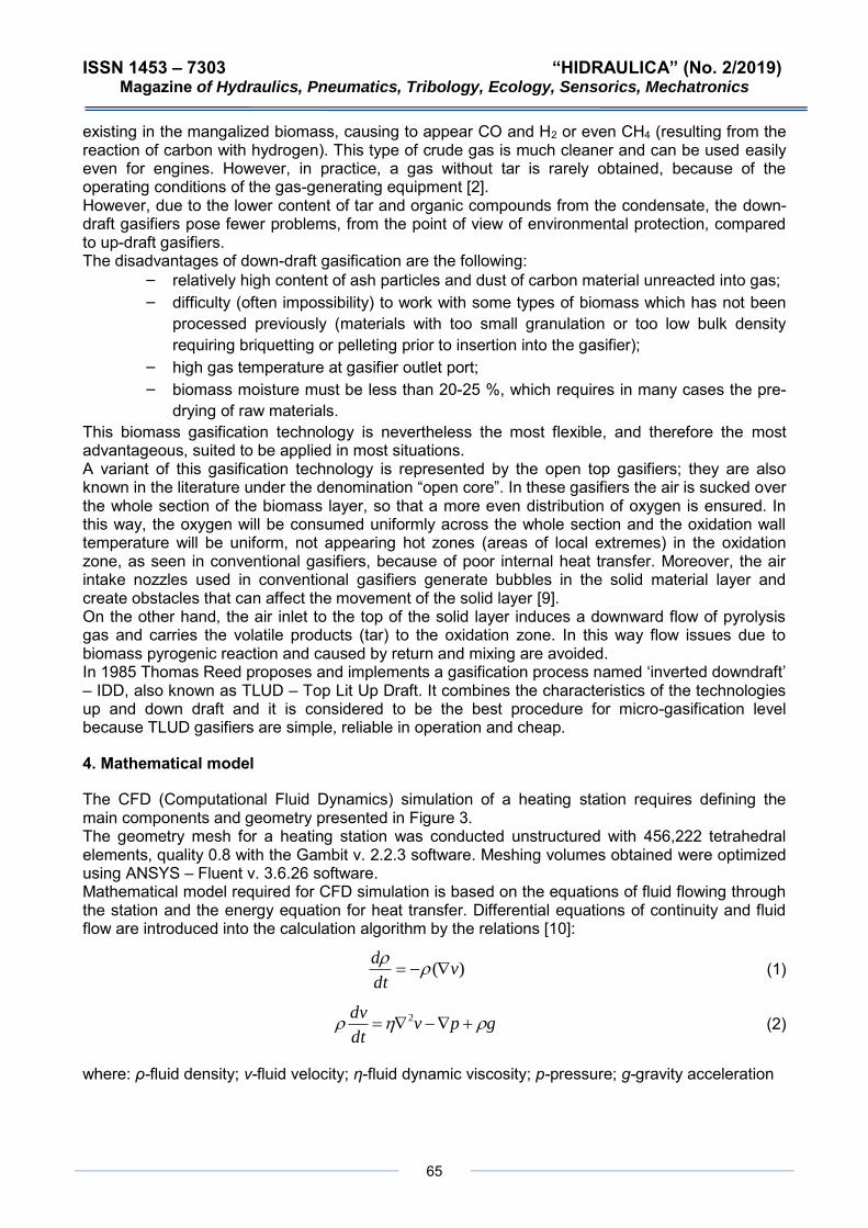
ISSN 1453 – 7303 “HIDRAULICA” (No. 2/2019) Magazine of Hydraulics, Pneumatics, Tribology, Ecology, Sensorics, Mechatronics
65
existing in the mangalized biomass, causing to appear CO and H2 or even CH4 (resulting from the reaction of carbon with hydrogen). This type of crude gas is much cleaner and can be used easily even for engines. However, in practice, a gas without tar is rarely obtained, because of the operating conditions of the gas-generating equipment [2]. However, due to the lower content of tar and organic compounds from the condensate, the down-draft gasifiers pose fewer problems, from the point of view of environmental protection, compared to up-draft gasifiers. The disadvantages of down-draft gasification are the following:
– relatively high content of ash particles and dust of carbon material unreacted into gas; – difficulty (often impossibility) to work with some types of biomass which has not been
processed previously (materials with too small granulation or too low bulk density requiring briquetting or pelleting prior to insertion into the gasifier);
– high gas temperature at gasifier outlet port; – biomass moisture must be less than 20-25 %, which requires in many cases the pre-
drying of raw materials. This biomass gasification technology is nevertheless the most flexible, and therefore the most advantageous, suited to be applied in most situations. A variant of this gasification technology is represented by the open top gasifiers; they are also known in the literature under the denomination “open core”. In these gasifiers the air is sucked over the whole section of the biomass layer, so that a more even distribution of oxygen is ensured. In this way, the oxygen will be consumed uniformly across the whole section and the oxidation wall temperature will be uniform, not appearing hot zones (areas of local extremes) in the oxidation zone, as seen in conventional gasifiers, because of poor internal heat transfer. Moreover, the air intake nozzles used in conventional gasifiers generate bubbles in the solid material layer and create obstacles that can affect the movement of the solid layer [9]. On the other hand, the air inlet to the top of the solid layer induces a downward flow of pyrolysis gas and carries the volatile products (tar) to the oxidation zone. In this way flow issues due to biomass pyrogenic reaction and caused by return and mixing are avoided. In 1985 Thomas Reed proposes and implements a gasification process named ‘inverted downdraft’ – IDD, also known as TLUD – Top Lit Up Draft. It combines the characteristics of the technologies up and down draft and it is considered to be the best procedure for micro-gasification level because TLUD gasifiers are simple, reliable in operation and cheap.
4. Mathematical model
The CFD (Computational Fluid Dynamics) simulation of a heating station requires defining the main components and geometry presented in Figure 3. The geometry mesh for a heating station was conducted unstructured with 456,222 tetrahedral elements, quality 0.8 with the Gambit v. 2.2.3 software. Meshing volumes obtained were optimized using ANSYS – Fluent v. 3.6.26 software. Mathematical model required for CFD simulation is based on the equations of fluid flowing through the station and the energy equation for heat transfer. Differential equations of continuity and fluid flow are introduced into the calculation algorithm by the relations [10]:
)( vdt
d−=
(1)
gpvdt
dv +−= 2 (2)
where: ρ-fluid density; v-fluid velocity; η-fluid dynamic viscosity; p-pressure; g-gravity acceleration

ISSN 1453 – 7303 “HIDRAULICA” (No. 2/2019) Magazine of Hydraulics, Pneumatics, Tribology, Ecology, Sensorics, Mechatronics
66
Fig. 3. Heating station geometry
1 – biomass burner;2 – furnace; 3 – heat exchanger; 4 – combustion air inlet port; 5 – outside air inlet port; 6 – hot air exhaust; 7 –
combustion gases exhaust.
Fig. 4. Unstructured mesh of heating station geometry for CFD simulation
Differential energy equation for calculating heat transfer is introduced into the calculation algorithm by the relation:
++
= TK
t
Q
dt
dU 2 (3)
where: U-internal energy; Q-heat flow; K-heat transfer global coefficient; T-temperature; θ-dissipation term. If the fluid is considered incompressible and unsteady, three equations above shall be simplified accordingly. From the flow conditions according to the formula of Reynolds there has been determined turbulent flow in the heat exchanger. The standard k-ε model is the simplest turbulence model with two transport equations, which are added to the three previous equations, allowing independent assessment of the turbulent velocity and the turbulence length scale. Values of turbulent kinetic energy k and dissipation velocity ε are obtained from the system of transport equations:
Mbk
ik
t
i
YGGx
k
xDt
Dk−−++
+
=
Pr (4)
( )k
CCGGk
CxPrxDt
D 2
2b3k1
i
t
i
−+
+
+
=
(5)
where: Gk-term for generation of turbulent kinetic energy; Gb-floatability term; YM -compressibility term; Prk and Prε -turbulent Prandtl numbers for k, and respectively for ε. Particularizing, the heat flow transmitted between the combustion gases and the air that has entered the heating station in the counter flow fluid-to-fluid heat exchanger, has the following equation:
mTSKQ = (6)
and capacity of the heating station shall be calculated using the next equation:
mpv TcqP = (7)

ISSN 1453 – 7303 “HIDRAULICA” (No. 2/2019) Magazine of Hydraulics, Pneumatics, Tribology, Ecology, Sensorics, Mechatronics
67
where: K-global heat transfer coefficient, S- heat transfer area, qv-volumetric flow rate, ρ- density; cp -specific heat; ∆Tm- temperature difference inside the station.
5. Experimental modeling and testing
The paper presents a modern way of preparing and using the vegetal biomass for the ecological production of the cheap thermal energy required in the heating installations technology specific to the rural economy based on agricultural activities. In a research project, an experimental model (Figure 5) was used which uses this procedure, which was tested in the laboratories of the institute. Thermal energy can be obtained by micro-gasification using the TLUD (Top-Lit UpDraft) process of vegetal biomass, which is characterized by high conversion efficiencies and very low CO and PM2.5 pollutant emissions. Applying the TLUD process it is possible to efficiently gasify biomass with relatively large variations of the chemical composition, humidity (under 20% water) and granulation properties (1-5 cm), aspect which provides a wide base of usable plant biomass sources [4]. The long-term acceptability of gasification technology and the CHAB concept as well as its introduction on the market depend on the technical performance, economic and environmental of gasification and biofuel plants, efficiency and safety of power plants that is using the gas fuel produced [6] In order to achieve these goals, the system must have high operational safety and be reliable, environmentally friendly, economically viable and be exploited by a user with a minimum of professional training trained carefully through a monitored schooling system. It is in the user and manufacturer's interest that the hot air generator is properly tested so as to achieve the desired performance. Therefore, a methodology has been developed for testing the hot air generator with the TLUD energy module, as well as calculation algorithms for the primary processing of experimental data. Testing is carried out in four test steps: 1. Initial running test for system components (IRT) 2. Start test (ST) (sensory training, measurement and control instruments, data acquisition components (ST) 3. Operational test of the biomass gasification process (LOT) 4. The biochar discharge and off test (BOT) The tests will be carried out in strict surveillance with the labor protection rules specific to hot combustion gases. Following the mathematical modeling of the equipment, the project was improved resulting the Prototype, Figure 5. The location of the heat exchanger and chimney fans is shown in fig. 6 and fig. 7. The micro-gasification process is supplied with air from a variable speed ventilator. Biomass is introduced into the reactor and is based on a grid through which, from bottom to top, passes the air for gasification. Initialization process is done from the free upper layer biomass. Thermal energy is obtained by burning hot gasogen, resulted during pyrolysis. It is mixed with preheated combustion air introduced into the combustion zone through holes located at the top of the reactor. Mixture with high turbulence burns with flame at the upper mouth of the generator with high temperature 900-1000°C. To adjust the heating power necessary, the air flow Dag for gasification and Dard for combustion are varied through two clacks, coupled mechanically or by varying ventilator speed. TLUD process is with fixed bed of biomass and therefore the generator operates in batch mode to recharging. In order to put the prototype of the TLUD hot air generator into operation, the reactor was filled with 15 kg of pellets and the ignition with 4 pieces of fireplaces igniters was used. The draft fan and the hot air fan ware started. After a start-up period, the gasification process stabilized and a stable, slightly turbulent flame of orange color was obtained. There was observed a high increase in air temperature at the outlet of the heat exchanger. After about 1 hour and 30 minutes, a total blue flame appeared at the burner, indicating the occurrence of gasification of the biochar. At that moment the blower stopped, the gasification and combustion

ISSN 1453 – 7303 “HIDRAULICA” (No. 2/2019) Magazine of Hydraulics, Pneumatics, Tribology, Ecology, Sensorics, Mechatronics
68
air were closed. At the complete extinction of the blue flame, the reactor was extracted from the generator and the biochar was discharged.
Fig. 5. TLUD thermal generator prototype equipped with heat-
resistant for temperature monitoring at points of interest
Fig. 6. Heat exchanger fan with a flow rate of 2000 m3 / h
Fig. 7. Smoke chimney fan with a flow rate of 605 m3 / h
In order to increase the technical performances of the TLUD hot air generator, compared to the Experimental Model, a number of modifications have been made to the prototype achievement: - supplying the heat exchanger with a fan with a flow rate of 2000 m3 / h, to reduce the temperature of the air conditioning (the air introduced into the greenhouse); - mounting on a chimney of a special construction fan with a flow rate of 605 m3 / h; -mounting of thermo-resistors (temperature probes) in the main monitoring points of the process of biomass gasification and gasification of gas from gas producing, fig. 8: probe 1-in ambient environment; probe 2 on the heat exchanger fan air supply duct; probe 3 on the flue gas exhaust manifold (coil), a fan that assures the unfolding of the biomass pyrolysis process by suctioning the bottom reactor air and passing it through the biomass; probe 4 on the hot air transport pipe to the greenhouse.
Probe 2
Probe 3
Probe 4
Fig. 8. Mounting points for thermo-resistors - the generator with the electric panel, fig. 9, which has been introduced: a programmable controller, which together with an external console allows real-time monitoring of recorded

ISSN 1453 – 7303 “HIDRAULICA” (No. 2/2019) Magazine of Hydraulics, Pneumatics, Tribology, Ecology, Sensorics, Mechatronics
69
temperature of thermo-resistors; a frequency converter that allows wide-ranging adjustment of fan speed installed on the chimney; -developing the software to enable the process of gasification and the monitoring of the working parameters.
Fig. 9. Electric panel of the heat generator; programming the monitoring system for working parameters and data acquisition
Densified solid biofuels used in experiments were pellets obtained from softwood species with a thermal efficiency of 5 kWh / kg, maximum length 45 mm, diameter 6 mm, humidity ≤ 10%, resulting ash content ≤ 0,7%. The pellets are introduced into the cylindrical reactor, fig. 10, which at the bottom is provided with a grill; after ignition of the pellets, by starting the fans, the primary air for gasification is determined to pass through the grill, passing through the ascending pellet mass. The pyrolysis process is triggered at a short time from the start of the fans, being sensed by the fact that at the top of the reactor, through the holes practiced in the circular sheath of the cover, intense burning of the gas from gas producing takes place, Fig. 11.
Fig. 10. The TLUD heat generator reactor Fig. 11. Referring to the moment of initiation of the
pyrolysis process The pyrolysis process results in gas from gas producing, tar and biochar. Tars pass through the incandescent charcoal layer, are cracked and totally reduced due to the heat radiated by the

ISSN 1453 – 7303 “HIDRAULICA” (No. 2/2019) Magazine of Hydraulics, Pneumatics, Tribology, Ecology, Sensorics, Mechatronics
70
pyrolysis front and the upper flame. The resulting gas is mixed with the secondary combustion air, preheated by the reactor wall, introduced into the combustion zone through the oriffices disposed at the top of the reactor. The mixture with high turbulence burns with flame at temperatures of about 900°C. The adjustment of the thermal power is made by the variation of the primary and secondary air flows. The experiments took place in two stages: - Stage I, which involved temperature monitoring at points of interest over a work cycle over time 1242-1349; the control elements during the working cycle were the gasification and combustion air intake valves; the reactor was fed with 7.9 kilograms of pellets; - Stage II, which involved temperature monitoring at points of interest over a work cycle over time 1404-1452; the adjustment elements during the working cycle were the gasification and combustion air intake valves, respectively the fan speed mounted on the chimney; the reactor was fed with 7 kg of pellets; Measured temperature values of heat-resistant are recorded at intervals of 30 s. The difference between the ambient temperature and the heat exchanger temperature is due to the fact that a mixture of ambient air and some of the air in the reactor enclosure takes place in the main fan pipe (heat exchanger fan). The Δt difference reflects the degree of heat recovery in the combustion gases, contributing to the increase in the efficiency of the heat generator. The graphical representation of the temperature values recorded during the two cycles of operation of the thermal generator is shown in the diagram of Fig. 12. The main objective of the experimentation of the equipment under actual operating conditions was that by the control elements (gasification and combustion clacks, frequency converter for regulating the speed of the gasification gas and the exhaust of the combustion gases), the temperature values should be maintained in Designed limits: Climate air temperature value to be maintained around 150°C, combustion gas temperature around 200°C, Δt value - the difference between the heat exchanger temperature and the ambient temperature to be as high as possible to increase the efficiency heat generator. In the case of the first operating cycle, only the burner clack at 13.14.49 was inserted in the direction of closing it, resulting in a limitation of the air temperature of the air at 177.5°C and of the combustion air temperature at 254°C. It is found that only by adjusting the aperture of the clacks the values of said temperatures can not be maintained at the projected values. In the second operation cycle, the gasification air flow rate was adjusted by changing the fan speed by means of the frequency converter. It is noted that the temperature of the air conditioning temperature was kept below 155.6°C, and the value of the combustion gases below 192°C.
Fig. 12. Graphic representation of recorded temperature values
during the two operating cycles of the heat generator

ISSN 1453 – 7303 “HIDRAULICA” (No. 2/2019) Magazine of Hydraulics, Pneumatics, Tribology, Ecology, Sensorics, Mechatronics
71
6. Conclusions
The prototype of the TLUD thermal generator, after removing the technical-functional deficiencies and the nonconformities found in the Experimental Model Test, meets the project objectives, works on the TLUD principle in different power regimes, achieves the projected values of the temperature at the points of interest and can be introduced into the fabrication delivered to the market. Adjustment elements (gasification and combustion clacks, frequency converter for regulating the gasification fan flow rate and flue gas exhaust) allow the temperature to be adjusted and maintained within the projected limits; To increase the efficiency of the heat generator, Δt - the difference between the temperature of the heat exchanger and the ambient temperature is higher; The value of the air temperature introduced into the greenhouse tubing can be brought to the desired value by mixing air conditioning with fresh air from the outside of the greenhouse through a clack pipe.
Acknowledgments This paper has been developed in INOE 2000-IHP, as part of a project co-financed by the European Union through the European Regional Development Fund, under Competitiveness Operational Programme 2014-2020, Priority Axis 1: Research, technological development and innovation (RD&I) to support economic competitiveness and business development, Action 1.2.3 – Partnerships for knowledge transfer, project title: Eco-innovative technologies for recovery of biomass wastes, project acronym: ECOVALDES, SMIS code: 105693-594, Financial agreement no. 129/23.09.2016.
References [1] Dumitrescu, Liliana, Cristescu Corneliu, Barbu Valentin, and Marinela Mateescu. “Combined system for
the production of thermal energy using solar and biomass energy”. Paper presented at ISB-INMA TEH' 2018 International Symposium, Bucharest, Romania, November 1 - 3, 2018.
[2] Gumz, W. Gas Producers and Blast Furnaces. John Wiley and Sons Inc., New York, 1950. [3] Belonio, A. Dual- reactor rice husk gasifier for 6-ton capacity recirculating-type paddy dryer. Central
Philippine University, Iloilo City, Philippines. [4] Mukunda, H., et al. ”Gasifier stoves – science, technology and field outreach.” Current Science 98, no. 5,
(March 2010). [5] Murad, E., A. Culamet, and G. Zamfiroiu. ”Biochar- Economically and ecologically efficient technology for
carbon fixing.” Paper presented at Hervex 2011 Symposium, Călimăneşti, Romania, November 9-11, 2011.
[6] Porteiro, J., D. Patino, et.al. “Experimental analysis of the ignition front propagation of several biomass fuels in fixed-bed combustor.” Fuel 89 (2010): 26-35.
[7] Varunkunar, S. “Packed bed gasification-combustion in biomass domestic stove and combustion systems.” Ph.D. thesis. Department of Aerospace Engineering Indian Institute of Science, Bangalore, India, 2012.
[8] Nazeer, W. A., L.M. Pickett, and D.R. Tree. ”In-situ Species, Temperature and Velocity Measurements in a Pulverized Coal Flame.” Combustion Sciences and Technology 143, no. 2 (1999): 63-77.
[9] Sinak, Y. ”Models and Projections of Energy use in the Soviet Union.” Chapter in Steiner, T. (ed.) International Energy Economics. Chapman and Hall, London, 1998: 1-53.
[10] Rowe, V. M. ”Some Secondary Flow Problems in Fluid Dynamics.” Ph. D. thesis. Cambridge University, Cambridge, UK, 1966.
