Royal Institute of Technology

Outokumpu Stainless AB

Examination of inclusion size distributions in duplex

stainless steel using electrolytic extraction

Master of Science Thesis

By

Siamak Shoja Chaeikar

Division of Applied Process Metallurgy

Department of Materials Science and Engineering

Royal Institute of Technology, SE-100 44 Stockholm, Sweden

May 2013

i

Abstract

Nowadays due to large demand for clean and defect-free steels, several techniques based on

different characteristics of particles are applied to investigate the steel cleanness. Outokumpu

Stainless AB in Avesta has performed extensive work in this field by applying several methods,

which all of them have specific advantages and limitations. However, it is necessary to find an

accurate technique to investigate real properties of inclusions in duplex stainless steels. For

routine analytical methods, calibration and parameters adjustment can be followed by help of

these investigation results.

The aim of present work is to apply automated INCA-Feature method for controlling cleanness

of LDX 6112 duplex stainless steels after electrolytic extractions (EE) as a reference method.

Three methods of investigations, INCA-Feature on polished samples as two-dimensional and on

film-filter as three-dimensional and EE as three-dimensional analyses, were compared. The

results of comparison between running INCA-Feature on polished samples and film filters show

an acceptable agreement which proves the possibility of performing EE on this steel grade and

using INCA-Feature for investigating this as a fast method. These methods are compared

statistically and quantitative results are reported in details.

ii

Acknowledgments

Hereby I would like to express my appreciation to Prof. Pär Jönsson who provided me great

opportunity to work at division of Applied Process Metallurgy. I also would like to offer my

special thanks to my supervisors Andrey Karasev and Jan Y. Jonsson for their support and their

incredible guidance during my work on this master thesis both in KTH and in Outokumpu

stainless AB. They also gave me many valuable instructions and suggestions for this thesis and I

learned a lot from them.

Last but not least, I am grateful to my family who has been always with me with endless love

and support.

iii

Contents 1. Introduction ........................................................................................................................................... 1

2. Theory ................................................................................................................................................... 2

2.1. Technological process and problems ............................................................................................ 2

2.2. Effect of inclusions on properties of final product ........................................................................ 4

2.3. Methods for investigating inclusions ............................................................................................ 7

3. Experimental ....................................................................................................................................... 10

3.1. Preparation of samples ................................................................................................................ 10

3.2. Electrolytic Extraction ................................................................................................................ 11

3.3. Preparation of samples for 2D investigation ............................................................................... 13

3.4. Investigation of inclusions .......................................................................................................... 14

3.4.1. SEM Investigations ............................................................................................................. 14

3.4.2. SEM-INCA Feature ............................................................................................................ 16

4. Results and Discussion ....................................................................................................................... 18

4.1. Effect of filter transportation on inclusions characteristics ......................................................... 18

4.2. Inclusion characteristics after EE ................................................................................................ 19

4.2.1. Homogeneity of particle distributions ................................................................................. 19

4.2.2. Morphology ......................................................................................................................... 20

4.2.3. Composition ........................................................................................................................ 23

4.2.4. Size and Number ................................................................................................................. 24

4.3. Inclusion characteristics after SEM investigations ..................................................................... 26

4.3.1. Comparison of EE+SEM and IF methods ............................................................................... 26

4.3.2. Comparison of EE+SEM and CS+IF methods ....................................................................... 30

4.4. Final comparison of different methods ...................................................................................... 32

5. Conclusions ......................................................................................................................................... 34

References ................................................................................................................................................... 36

APPENDIXES ................................................................................................................................................ 37

1

1. Introduction

Because of growing demand of clean and defect-free steels, offline and online determination of

inclusions have become more essential in modern industry. Criteria of steel cleanness are set by

measuring amount of impurities and inclusions in final product. As a result, applying an

appropriate and fast method to investigate inclusions plays a significant role in today’s

technology.

There is a wide variety of techniques to investigate steel cleanness, based on different

characteristics of particles. Outokumpu Stainless AB in Avesta has performed extensive work in

this field by applying several methods, for examples Optical emission spectroscopy with pulse

distribution analysis technique, PDA-OES, wet chemistry and Scanning electron microscopy

together with INCA-Feature. While each of these techniques has its own advantages and

limitation, finding a suitable method to characterize real properties of inclusions in duplex

stainless steels is a main interest. Results of such method can help to calibrate or adjust

parameters of routine methods in this plant.

The aim of present job was to optimize the INCA-Feature method for controlling cleanness of

duplex stainless steels. Electrolytic extractions (EE) as a reference method were performed on

samples at KTH and then film filters were transported to Avesta for scanning with SEM-Feature.

Automated SEM measurements were run on the film-filters and polished plate samples, while

same film-filters were investigated by SEM manually. Results of investigations with different

methods including two-dimensional and three-dimensional analysis were compared; the results

can further improve the methods of investigating non-metallic inclusions. The effect of

transportation on the film-filters was also examined.

The duplex stainless steel grade selected for this project was LDX 2101which is named as

6112in Avesta internal production and also in this report. Sampling was done based on different

pattern of inclusions types to compare several aspects and optimize SEM in the best way. Since

EE is a three dimensional method for investigating inclusions, the results of this work can also be

applied for improving other methods like PDA. So, in future works PDA results can be

interpreted regarding inclusion size distribution in duplex stainless steels with help of electrolytic

extraction (EE).

2

2. Theory

In this chapter, process of steelmaking at Outokumpu AB. in Avesta in introduced to give a

perspective about possible inclusions formed during this process. In second section a literature

review on effects of inclusions on properties of final product in presented which will help to

understand the importance of investigation steel cleanness. In last section the methods applied

for these investigations will be discussed.

2.1. Technological process and problems

In modern industry, steel producers attempt to improve steel making process to gain the best

quality and cleanliness of final product; while cleanness means lowest possible level of

impurities in steel. The steel making sequence is planned based on the steel grade, composition

and final required properties, meanwhile some steps are in common for all grades in different

steelmaking methods. The present method to produce stainless steels at Outokumpu is a scrap-

based steelmaking process. There are four main steps in this method: a) electric arc furnace

(EAF), b) argon oxygen decarburization (AOD), c) ladle furnace (LF) and d) casting. A

schematic of this process is shown shortly in figure 1 [1], which will be discussed in more details

in this chapter.

Fig. 1- Schematic of Steelmaking process at Outokumpu Stainless Avesta

3

First furnace should be filled with the scraps, and then the arc starts from a spot on the cathode,

expands to a cone and ends at the anode. The temperature in the middle of arc can reach

temperature between 25000-30000 °C while radiation heat from the arc is used to melt scrap and

melt has temperature from 1500 to 1600 °C. Melting will be finished when all scraps from each

scrap variety are melted, steel analysis is correct and the amount of energy is consumed. The

process time is around 60 minutes and temperature is controlled to be almost 1650 ° C.

Thereafter furnace is tilted and melt is tapped into the ladle.

In second step, AOD convertor, decarburization, reduction and chemical analysis adjustment is

performed on the steel melt. The converter step consists of two steps: Decarburization in which

carbon content of the steel reduces by means of injecting oxygen and inert gas, Re-Reduction of

chromium, manganese and iron which are oxidized in the slag and should be taken back to the

melt. For this step a reducing agent, mostly Si or Al from converter’s top is added which reacts

with metal oxides in the slag. Carbon content changes from 0.5-2.0%. to 0.02-0.1% after AOD

step.

In ladle furnace chemical analysis of steel is adjusted. In ladle an arc is formed by three graphite

electrodes close to melt while in order to protect ladle against arcs, a slag layer is required. The

alloys are added in pieces form or as wire filled with alloys in powder form based on sampling

results and composition calculations. The melt is stirred during whole process to obtain a

homogeneous mixture.

Last step is continuous casting machine, in which molten metal is drained from the tundish

through a copper mold. The mold is water-cooled to solidify the hot metal directly in contact

with it. In this step in order to have the most appropriate solidification quality and final

microstructure, temperature control is so important. In order to reduce heat losses, ladle is lined.

The steel surface is protected by a slag layer and an insulating ladle lid. The inclusions remained

from last steps should be removed in the tundish. Meanwhile, the steel melt is protected against

oxygen to prevent formation of new inclusions. It is also important that the tundish is properly

lined and conduit, so that no oxygen leaks into it and new inclusions are not formed [2].

4

2.2. Effect of inclusions on properties of final product

Two specific types of nonmetallic inclusions are formed in steels during process which are

named indigenous inclusions or exogenous inclusions according to their origin. Indigenous

inclusions are formed as a result of deoxidization or precipitation during cooling and

solidification. Deoxidization products, for example alumina and silica inclusions are mostly

formed due to reaction between the dissolved oxygen and the deoxidant agent, such as aluminum

and silicon. Alumina inclusions can have dendritic, cluster-type or coral-like morphologies

(Figure 2) based on the oxygen content in environment to react with Al present in steel melt [3].

Fig. 2- different morphologies of alumina inclusions formed due to deoxidization: (A) dendritic and clustered

alumina (B) alumina cluster and (C) coral-like alumina

Silica inclusions have spherical shape, while they can also agglomerate and form clusters, as

shown in Figure 3. These inclusions nucleate a bit after adding deoxidizer and then grow fast.

Inclusion growth can be controlled by diffusion of the deoxidization elements and oxygen

content [3].

Fig. 3- spherical morphology of silica inclusions

Exogenous inclusions can appear while chemical or mechanical interaction happens between

liquid steel and its surroundings. Some cases include getting trapped of a slag particle in steel

A) B) C)

5

melt and exogenous inclusions start to nucleate and grow on this impurity, lining erosion (Figure

4), and chemical reactions. These inclusions are dispersed in steel and since they flow easily, are

most concentrate in rapid solidified regions, which is near the ingot surface. They mostly have

multi-compound/phases compositions, large size, Irregular shape, small number and low volume

fraction, dispersed distribution in the steel and so deleterious effect on steel quality. Their source

can be identified by investigating their shape, size and composition [4].

Fig. 4- Exogenous inclusions due to A) trapped slag particle in steel melt and B) lining erosion

As was mentioned in beginning of this chapter, properties of final product is significantly

affected by mechanical behavior of inclusions during steel processing. They generally have a

deleterious effect on machinability, surface quality, and mechanical properties [4].

This effect during deformation is schematically illustrated in figure 5 [5]. It can be seen that the

“Stringer” formation defect, anisotropy in mechanical properties and decreasing toughness and

ductility can be caused by such particles during metal forming. The worst situation happens

when inclusions are located through thickness direction [3].

A) B)

6

Fig. 5- Schematic illustration of effect of inclusions on steel properties during metal forming

It is also shown that inclusions can have detrimental effects on the ductility of steel at hot-

working temperatures [6]. While different types of inclusions can have different effects on these

properties, Sulfides do not arise problems in hot working in majority of steels. But oxide-type

inclusions have a much greater influence on ductility at hot-working temperatures. In the case

that tensile stresses are applied in hat-working process, e.g. rotary piercing and open-die forging,

a cleaner steel will be required [7].

Inclusions also have been considered as one of the main reasons for fatigue failure in steels, so, if

fatigue strength under dynamic loading is required, cleanness of steels is seriously controlled [8].

Non-metallic inclusions reduce the fatigue strength and endurance [9] while hard and brittle

oxide inclusions are the most harmful [10]. Oxysulfide inclusions are less deleterious than

single-phase alumina and/or calcium oxides due to since presence of a more deformable sulfide

phase, mostly as MnS [11].

Hard particles like inclusions can also cause ductile fracture in steels while nucleation, growth,

and coalescence of voids can happen in the location of these particles, pearlite nodules and

carbides. In this case, inclusions are harder than the matrix which leads to the stress

(a) A “HARD” INCLUSION UNDER

ROLLING CONDITIONS

(b) A “HARD” CRYSTALLINE INCLUSION

BROKEN DURING ROLLING

(c) A “HARD” INCLUSION CLUSTER

“STRUNG OUT” DURING ROLLING

(d) AN INCLUSION COMPOSED OF

“HARD” CRYSTALS DISPERSED IN A

“SOFT” MATRIX

(e) A “SOFT” INCLUSION UNDER

ROLLING CONDITIONS

BEFORE ROLLING

AFTER ROLLING

CAVITY

7

concentration during matrix deformation and finally forming of voids. The harmful effects will

be more serious if the inclusions consist of hard and brittle oxides. The size of inclusions has also

a great importance, while for particle size below a minimum limit voids will not form. Smaller

volume fraction of inclusions and control of the inclusion shape will improve the mechanical

properties, for example Charpy energy and fracture toughness [8].

Since inclusions affect the fatigue strength and fracture behavior of steels, they also can

decrease service life of steel components [12].

2.3. Methods for investigating inclusions

Considering the harmful effects of inclusions on steel quality which was discussed in last

section, a strict control of cleanness is necessary in terms of the number, composition,

morphology, and distribution of oxide particles [13].

In characterization of inclusions in steels, several parameters can be investigated, e.g.

quantitative parameters, shape, distribution, chemical composition and specific properties.

Methods for the investigating inclusions can be listed as follows:

- Optical and electron microscopy investigations

- Non-destructive testing

- Ultrasonic tests

- Magnetism-related techniques

- X- ray transmission

- Inclusion concentration methods

- Chemical analysis

- Fracture methods

- Oxygen determination

- Spark emission

- Statistical prediction [8].

The methods applied in this work are Electrolytic Extraction (EE) and Scanning Electron

Microscopy (SEM) with INCA-Feature technique. Their principle and output data will be

discussed in detail in this chapter.

8

Inclusions are subdivided into macro- (>20 μm), micro- (1–20 μm) and sub-micro inclusions (<1

μm) and in general it is not possible to analyze all sizes of inclusions at the same time. Figure 6

illustrates employed techniques together with the SEM-Feature method applied for cleanliness

investigations, possible size range of each method is also shown.

Fig. 6- Size range of inclusions investigating techniques and usual size distribution of inclusions

This figure indicates two important advantages of the automated SEM-Feature unit, which is that

both range of size detection limit and the numbers of detectable inclusions are large. This method

produces a large quantity of raw data which will be then processed by offline software.

Sample preparation of this method is the same as metallographic preparation technique. The

instrument of inclusion analysis is a conventional scanning electron microscope (SEM) with

secondary electron (SE), back-scattered electron (BSE) and a drifted energy-dispersive silicon X-

ray detector (EDX) for determining chemical composition of inclusions.

By using the software samples can be analyzed completely automatically by identifying a user-

defined area to be scanned for detecting non-metallic inclusions. The area of high atomic number

is appeared brightly in BSE-mode contrast while low atomic number is displayed darkly, e.g.

non-metallic inclusions.

Dark features are defined based on a threshold criterion in pixel intensity. When particles are

detected by scanning each field of area, EDX spectrum will measure the elemental composition

of the particle.

9

On the basis of the determined elemental composition criterion, features will be identified or

rejected and then excluded online.

An offline evaluation program can also be used afterwards to classify the detected particles into

inclusion classes. A content of iron is always introduced in chemical composition of particles,

because X-rays are not only emitted by the inclusion but also matrix. The smaller the detected

particle the larger is the iron content in the spectrum. This error can be modified by removing

iron content and normalizing.

For classification the renormalized data will be applied and other particles will be excluded. The

software also calculates the diameter of a circle with equal area and the length/width ratio which

gives the size and shape of each particle, respectively [14]. This is a two dimensional method

which is used as an applicable technique in steel making plants, including Outokumpu Stainless

in Avesta.

The principle of EE technique is different solubility of elements and phases in an electrolyte. A

cubic piece of samples is dissolved in an electrolytic solution composed while an electric current

is applied. Current and electrolyte should be selected in such a way that matrix and other

particles, e.g. carbides, are dissolved but inclusions are remained. After dissolution for a specific

time, depending on applied current, the solution is filtered and undissolved particles are collected

on a film filter. These films are then investigated by SEM to measure inclusions characteristics.

This is a three dimensional method which needs ling time but results are so accurate and close to

original properties of particles.

10

3. Experimental

3.1. Preparation of samples

The sampling procedure was made in Outokumpu Stainless AB Company (Sweden). Four

duplex stainless steel samples were taken from the grade LDX 2101, internally named as 6112.

Chemical analysis of this grade is illustrated in Table 1.

Table 1- Chemical composition of duplex stainless steel grade LDX 2101(6112)

Steel C Si Mn P S Cr Ni Mo Al B

6112 0.025 0.70 5.00 0.035 0.002 21.50 1.55 0.30 0.025 0.002

Previous inclusions analysis data obtained by the company on the plate samples show that these

samples have four different inclusions pattern on their SiO2-(MgO,CaO)-Al2O3 ternary diagrams

(See Appendix 1). The samples were chosen based on these differences in order to cover all

kinds of inclusions.

The plate samples were taken from final coiled products and they were cut from the beginning or

end of the coils. Table 2 shows list of the samples including their detailed parameters and the

experiments have been done on each sample.

Table 2- List of samples including summery of performed investigations

Heat No.

Al (wt%)

Location of Sample

Plate thickness

(mm)

Charge No.

Sampling Zone in

coil Investigations

405519 0,011 Center

5 413634 End *

Section *

405523 0,02 Center

5 413550 End *

Section *

401931 0,024 Section 10 412999 Begin *

LDX 60505

0,003 Center

5 413841 Unknown *

Section *

*EE (electrolytic extraction), INCA (2D), INCA (3D), SEM-Manual (3D)

Longitudinal cross section (henceforth zone A) and center of each plate (henceforth zone B)

were prepared for investigations by SEM and electrolytic extraction (henceforth EE). In order to

have good comparison between different methods of investigation, it is needed that

characteristics and distribution of inclusions do not change in analyzing area. To fulfill this, both

11

section and center samples were mechanically cut to be safe from overheating and areas for

analyzing were selected near to each other as schematically illustrated in figure 7.

Fig. 7- Schematic illustration of analyzed areas in (A) cross section (zone A) and (B) in center samples (zone B)

As it can be seen, selected areas for SEM investigations on plate (2D) and EE investigations

(3D) in section and center samples were selected near to each other.

3.2. Electrolytic Extraction

In order to obtain the size distribution and avoiding that large inclusions are not extracted, it is

important to dissolve an adequately thick steel layer. After extraction of steel samples and

filtration of solution, different kinds of inclusions characteristics (such as size distribution,

composition, morphology) in steel can be determined by 3-D analysis of inclusions. This

analysis was carried out by scanning electron microscopy (SEM) after electrolytic extraction of

metal specimens. Based on the obtained data it is possible to get reliable particle size distribution

(PSD), composition and morphology of non-metallic particles.

For performing EE, samples from steel plates were cut into smaller specimens. HCCS samples

are about 11-14 × 11-14 × 2-5 mm (l × w × t) and VCS samples have almost same dimensions

but with the thickness of 5-10 mm.

The principle of EE method is dissolution of metal matrix in electrolyte by applying electric

current. The schematic illustration of equipment for EE (a) and filtration (b) are shown in Figure

8.

A) B)

Zone A

Zone B Vertical Cross

Section (VCS)

Horizontal Center Cross

Section (HCCS)

12

Fig. 8- Schematic illustration of (A) electrolytic extraction of metal sample and (B) filtration of solution

The EE process extracts the non-metallic particles from metal specimens. After extraction, the

electrolyte containing inclusions is filtered. By applying different extraction setting, it is possible

to reach the desirable depth of dissolved layer of the metal sample and desirable amount of

inclusions on the film filter.

Before EE and after removing all the possible oxidation products from surfaces by grinding

mechanically, all specimens were treated in ultrasonic bath and then cleaned by acetone and

petroleum benzene. The weight of steel specimens was measured before and after extraction in

order to determine the weight and volume of dissolved metal. The desirable surface for EE was

marked and all other surfaces were covered by a polymeric insulator to prevent dissolution of

other surfaces. The potentiostatic electrolytic extraction of metal samples, were carried out at

following parameters: electric charge ̶ 500 and 1000 Coulombs, voltage ̶ 5V, electric current ̶

20~50 mA, electrolyte 10%AA which is composed of methanol, 10v/v% acetylacetone and

1w/v% tetramethylammonium chloride. Detail of EE parameters applied on the samples is

shown in Table 3.

A) B)

13

Table 3- Electrolytic extraction parameters applied on metal samples

Sample NO.

Zone Electric charge

(Coulombs)

Dissolving area (mm2)*

Total dissolved metal (g)

Depth of dissolution

(mm)

405519 B 1000 183.2 0.2415 0.1707

A 500 61.5 0.0789 0.1661

405523 B 1000 168.7 0.2313 0.1775

A 500 64.4 0.092 0.1850

401931 B 1000 160.9 0.2166 0.1743

A 500 120.3 0.1035 0.1115

LDX 60505

B 500 177.4 0.1206 0.0881

A 500 72 0.1212 0.2181

*Samples were extracted from one surface

After electrolytic extraction, the obtained solution containing inclusions is filtered using a

polycarbonate membrane filter (PC) with an open-pore size of 1 µm. The solution goes through

the filter with the help of an aspirator. After filtration, inclusions are collected on the film filter

and can be investigated in SEM.

3.3. Preparation of samples for 2D investigation

When preparing plate samples for two-dimensional (2D) investigations by scanning electron

microscope, water-base suspensions and coolants should be generally avoided since water may

damage or dissolve some inclusions. In order to prevent inclusion dissolutions in water and to

keep the original and true chemical composition of the inclusions, all the samples were prepared

water-free. Samples prepared by this method were investigated by scanning electron microscope

and INCA feature. INCA feature system will automatically be able to separate scratches and dust

from real features but by providing a surface free from artifacts, analysis time will be

significantly reduced.

In the first step of preparation, samples were fixed in a steel fixture on an even and flat area.

Then they were roughly grinded for about 30 seconds. In this step water was used as coolant

during grinding. Then in the MD-Allegro machine they were finely grinded up to 9μm with

ethanol and diamonds solution for 288 seconds. A maintenance-free composite disc with

diameter of 300 mm was used, which magnetically fixed on the machine.

In the second step, plate samples were polished up to 3μm with a MD-plus machine for 360

seconds for two times. A synthetic nap dry disc with diameter of 300 mm and suspension of

14

water free diamonds with ethanol were used. Then samples were washed with ethanol and dried

with hot air.

In the last step, samples were polished with MD-Chem machine for 210 seconds. In this step a

porous and dry Neoprene disc with the diameter of 300 mm. Final polishing step was performed

with suspension of 0.2 µm water-free silica abrasive particles with ethanol. This is critical for

soft and annealed steels to avoid preparation artifacts. Finally samples were washed with ethanol

and dried with hot air.

3.4. Investigation of inclusions

3.4.1. SEM Investigations

The scanning electron microscope (SEM) makes image of the sample surface by scanning it with

high-energy beam of electrons in a raster scan pattern. The electrons interact with the sample

atoms, producing signals that contain information about the sample surface topography,

composition and other properties such as electrical conductivity. The types of signals produced

by SEM include secondary electrons, back-scattered electrons (BSE), characteristic X-rays, light

(Cathodoluminescence), specimen current and transmitted electrons. With secondary electrons,

sharp surfaces and edges tend to be brighter than flat surfaces and the topography of the sample

can be observed. Back-scattered electrons are used to localize objects for energy-dispersed

spectra (EDS) analysis. Back-scattered electrons help to differentiate between phases, showing

them in a range of grey levels. The grey level image is then used by the system to detect objects

and to analyze their geometry and chemistry. The back-scattered electron depth may affect the

size of an object such that it appears slightly bigger in the image [15].

After electrolytic extraction and filtration, the inclusions are analyzed on surface of the film-filter

by SEM (Zeiss Ultra55, FEG). A piece of film-filter was cut and pasted on a conductive carbon

tape and it pasted on an aluminum holder. For observation and EDS analysis, the BSE mode with

15 kV and the working distance of 8mm is chosen. In all samples 10 pictures are taken randomly

from top to the bottom of the film filter and the magnification of 1000X is used. Figure 9 shows

schematic illustration of the film-filter and the observed zones.

15

Fig. 9- Schematic illustration of investigated zones on the film filter

SEM images are taken in different zones from top to the bottom of the film filter in order to have

representative results and also not to count an inclusion twice. By the use of EDS, oxide

inclusions are distinguished from other particles for further analysis.

When oxide inclusions are distinguished on SEM images, equivalent diameter of the particles is

determined manually as shown in Figure 10.

Fig. 10- Length and width measurement for determining equivalent diameter of particles

For determining equivalent diameter of regular and irregular particles, equation (1) is used.

dv = √W × L (1)

For spherical inclusions the equivalent diameter is also measured. A list with every inclusion and

their diameter is obtained. For determination of particle size distribution, the total number of

inclusions per cubic millimeter, Nv, was calculated by using equation (2).

Nv = nAf

Aobs

ρme

∆W (2)

W L

Random micrographs taken

on the surface of film filter

16

n: number of particles within the size range

Af: total filter area with inclusions (1486 mm2)

Aobs: Observed area on SEM pictures

ρme: Metal density (ρme= 0.00772 g/mm2)

ΔW: Weight of dissolved metal during electrolytic extraction (g)

3.4.2. SEM-INCA Feature

Manual detection and characteristics measurement of the inclusions are very slow and time

consuming. INCA Feature (IF) is a dedicated solution for automated detection and analysis of

the inclusions. It can automatically determine the particles and gives very detailed analysis of the

particles. INCA Feature uses image processing software together with EDS analysis to

distinguish the particles based on their geometrical and chemical composition characteristics.

After defining a pattern like a rectangle, circle, line, point, etc., software divides the area into a

series of smaller fields. Then for each field it takes a micrograph and detects the objects and does

the particle analysis (see figure 11). Finally, a list is made that points out each particle on the

micrograph and also gives other characteristics related to that specific particle. Figure 11a)

illustrates position of electron gun, EDS detector, stag and defined pattern for analysis. Figure

11b) show the rectangle area which is defined on a mechanically polished sample and divided

into smaller grids and dots illustrate distribution of oxide inclusions on that area. Figure 11c)

shows two areas that are defined on two different points of the film-filter and distribution of all

particles which are detected on them.

Fig. 11- schematically illustrates a) position of investigating area respective to the electron gun and EDS detector b)

distribution of inclusions on a polished sample and c) distribution of all particles on two points of the film-filter

A) B) C)

17

In this study IF was used for analyzing the inclusions on both mechanically polished plate

samples and gold plated film-filters. For two-dimensional analysis of inclusions on mechanically

polished plate samples a rectangle with the area of 10-12mm2 was defined on each sample (see

figure 11b). Following feature functions for detection setup are used for running IF on polished

late samples:

Magnification: 1000X

Image size: 2048×2048 px

Minimum inclusion size: (px/ecd): 20 / 0.63 µm

“Median” filter before Auto Threshold

Since surface of the gold plated film-filter is not totally flat and it is not possible for the software

to focus on its surface automatically, then for running IF on the film-filter ten points were

defined and manually focused from top to the bottom of the film-filter. Total analyzing area is

about 0.7 mm2 and following feature functions for detection setup were also used for performing

IF on gold plated film-filters:

Magnification: 1000X

Image size: 2048×2048 px

Minimum inclusion size: (px/ecd): 20 / 0.63 µm

Three “Median” filters before auto threshold and “Hole Fill” and “Close” filters after

thresholding

18

4. Results and Discussion

4.1. Effect of filter transportation on inclusions characteristics

After electrolytic extraction in laboratory at KTH in Stockholm, film filters should be transported

to Avesta in order to do electron microscope investigations. During this transportation particles

can move on the surface of the film filter making a non-homogenous distribution and as a result

a real particle size distribution cannot be calculated. To prevent or minimize movement of the

particles on the surface of film filters, they were coated by a thin gold layer. This coating layer

also makes the surface more conductive and gives better brightness and contrast during SEM

investigations. While transporting, samples were fixed in the container and tried not to be shaken

or tilted. In order to investigate this transportation effect on the particles, before transportation

ten photographs were taken from top to the middle of the one of the film filters at the

magnification of 1000X and then same photographs from the same area also were taken after

transportation in Avesta with another SEM instrument.

Two of these photographs that were taken on the same fields of the film filter before and after of

transportation, are shown in figure 12.

Fig. 12- Particles on film filter, before (A&C) and after (B&D) transportation on fields number 6 (A&B) and 7

(C&D)

A) B)

C) D)

19

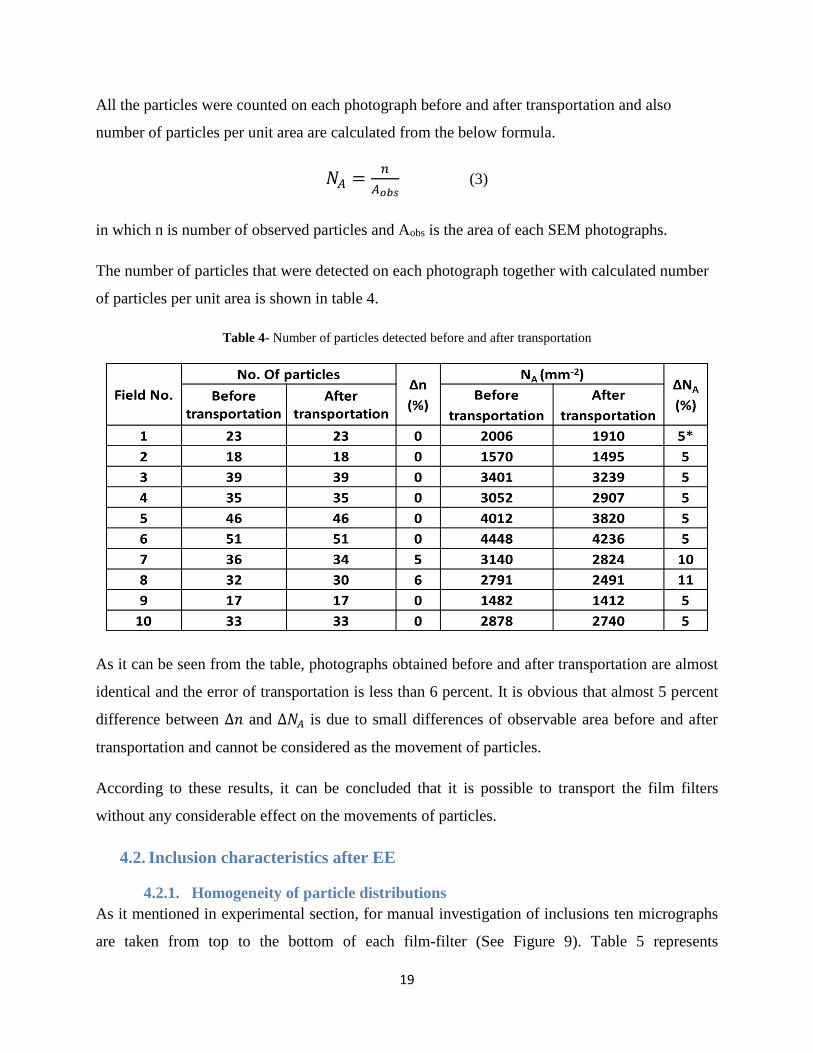
All the particles were counted on each photograph before and after transportation and also

number of particles per unit area are calculated from the below formula.

𝑁𝐴 =𝑛

𝐴𝑜𝑏𝑠 (3)

in which n is number of observed particles and Aobs is the area of each SEM photographs.

The number of particles that were detected on each photograph together with calculated number

of particles per unit area is shown in table 4.

Table 4- Number of particles detected before and after transportation

As it can be seen from the table, photographs obtained before and after transportation are almost

identical and the error of transportation is less than 6 percent. It is obvious that almost 5 percent

difference between ∆𝑛 and ∆𝑁𝐴 is due to small differences of observable area before and after

transportation and cannot be considered as the movement of particles.

According to these results, it can be concluded that it is possible to transport the film filters

without any considerable effect on the movements of particles.

4.2. Inclusion characteristics after EE

4.2.1. Homogeneity of particle distributions

As it mentioned in experimental section, for manual investigation of inclusions ten micrographs

are taken from top to the bottom of each film-filter (See Figure 9). Table 5 represents

20

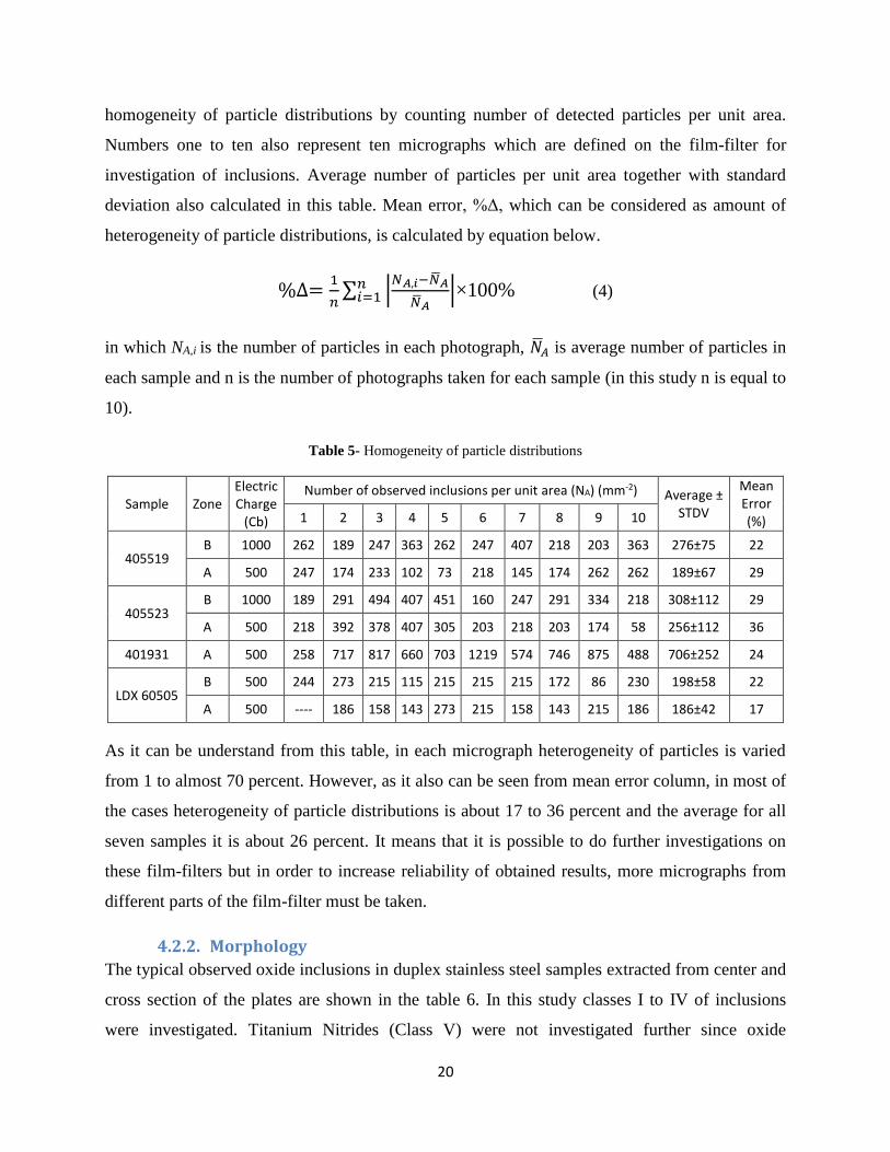
homogeneity of particle distributions by counting number of detected particles per unit area.

Numbers one to ten also represent ten micrographs which are defined on the film-filter for

investigation of inclusions. Average number of particles per unit area together with standard

deviation also calculated in this table. Mean error, %Δ, which can be considered as amount of

heterogeneity of particle distributions, is calculated by equation below.

%∆=1

𝑛∑ |

𝑁𝐴,𝑖−�̅�𝐴

�̅�𝐴|𝑛

𝑖=1 ×100% (4)

in which NA,i is the number of particles in each photograph, �̅�𝐴 is average number of particles in

each sample and n is the number of photographs taken for each sample (in this study n is equal to

10).

Table 5- Homogeneity of particle distributions

Sample Zone Electric Charge

(Cb)

Number of observed inclusions per unit area (NA) (mm-2) Average ± STDV

Mean Error (%) 1 2 3 4 5 6 7 8 9 10

405519 B 1000 262 189 247 363 262 247 407 218 203 363 276±75 22

A 500 247 174 233 102 73 218 145 174 262 262 189±67 29

405523 B 1000 189 291 494 407 451 160 247 291 334 218 308±112 29

A 500 218 392 378 407 305 203 218 203 174 58 256±112 36

401931 A 500 258 717 817 660 703 1219 574 746 875 488 706±252 24

LDX 60505 B 500 244 273 215 115 215 215 215 172 86 230 198±58 22

A 500 ---- 186 158 143 273 215 158 143 215 186 186±42 17

As it can be understand from this table, in each micrograph heterogeneity of particles is varied

from 1 to almost 70 percent. However, as it also can be seen from mean error column, in most of

the cases heterogeneity of particle distributions is about 17 to 36 percent and the average for all

seven samples it is about 26 percent. It means that it is possible to do further investigations on

these film-filters but in order to increase reliability of obtained results, more micrographs from

different parts of the film-filter must be taken.

4.2.2. Morphology

The typical observed oxide inclusions in duplex stainless steel samples extracted from center and

cross section of the plates are shown in the table 6. In this study classes I to IV of inclusions

were investigated. Titanium Nitrides (Class V) were not investigated further since oxide

21

inclusions were more important for the company. It must be also mentioned that since La-Ce

particles (Class III) are heavy particles they have almost same brightness as metallic matrix on

SEM and could not be detected on mechanically polished plate samples very easily, but because

of their brightness they can be easily detected on the surface of the film-filters.

Table 6- Typical morphology, composition and frequency of observed inclusions after EE

Class Typical Image Size Chemical Frequency of

range (µm) composition inclusions (%)

I

1≤dv≤3.8 Al-Ca-(Mg)-O ~8-32

II

0 .8≤dv≤1.7 0.7≤dv≤3

Mg-Al-O Mg-O, Al-O

~1-7 ~8-21

III

3≤dv≤7 La-Ce-Al(Si)-O ~6-11

IV

2≤dv≤6 Mg-Ca-O+TiN

Al-Ca-Mg-O+TiN ~5-13

V

0.8≤dv≤3 Ti-N ~19-32

Inclusions observed on the film-filter were classified into three categories of spherical, regular

and irregular depending on the morphology. Since in manual investigation particles can be

observed and detected by human, so there would be no difficulty for dividing them into these

22

three groups. Yet, with this method, automated discrimination of particles based on the

morphology is not possible. To be able to distinguish approximate morphology of the particles

from IF results, following equations were defined based on experimental observations:

I. Spherical : Aspect Ratio(Length

Breadth) < 1.5 and Circularity factor (

Perimeter2

4π×Area) = 1.0~1.1

II. Regular : Aspect Ratio(Length

Breadth) > 1.5 and Circularity factor(

Perimeter2

4π×Area) = 1.1~1.3

III. Irregular : Aspect Ratio(Length

Breadth) > 1.5 and Circularity factor (

Perimeter2

4π×Area) > 1.3

By applying above definitions, morphology of particles in automated methods can be compared

with manual observation which can be considered as real morphology of particles. Frequency of

particles with same morphology category is shown in figure 13. In this figure, percentage of

inclusions in different samples calculated by manual investigations on the micrographs obtained

after electrolytic extraction.

Fig. 13- Frequency of spherical, regular and irregular inclusions for all samples

It can be recognized that frequency of spherical incisions is more than two other shapes. This

amount for spherical inclusions is about 50-95 percent while for regular and irregular shapes are

less than 40 and 30 percent respectively. This data also can represent the possibility of

performing electrolytic extraction on this special grade of duplex stainless steel.

0

10

20

30

40

50

60

70

80

90

100

Spherical Regular Irregular

Am

ou

nt

of

incl

usi

on

s /p

ct

23

4.2.3. Composition

General composition of particles in the steel grade 6112 together with their frequencies will be

discussed in this section. Table 7 briefly shows the frequency of different types of particles

observed in this steel grade for all samples. In must be mentioned that one of the difficulties and

limitations of applying electrolytic extraction on this grade of duplex stainless steel and INCA-

Feature on the film-filter is the amount of scrap particles compared to the amount of inclusions

which should be detected by EDS method. In these samples 63-75% of the particles were scrap

particles consisting of un-dissolved metal matrix, phases and carbides. In table 7, scrap particles

are excluded and frequency of other particles is normalized to hundred percent.

Table 7- Frequency of different types of particles observed in steel grade 6112

Sample Location Oxide

(%) Sulfide

(%) Oxysulfide

(%) Nitride

(%)

405523 B 57.4 0.3 1.5 40.7

405523 A 37.0 1.6 2.2 59.2

405519 B 27.5 0.3 1.1 71.1

405519 A 27.0 0.5 0.8 71.6

401931 A 78.3 0.3 1.5 19.9

LDX60505 B 23.3 0.0 1.1 75.6

LDX60505 A 25.6 0.4 3.8 70.3

Average 39.5 0.5 1.7 58.4

STDV 20.8 0.5 1.0 20.7

Average frequency of particles and the standard deviations are plotted in figure 14. It can be

noticed that average frequency of oxide inclusions after normalizing is about 39 percent while

frequency of nitrides is about 58 percent. In these samples less than 3 percent of the particles are

sulfides and Oxysulfides and that is due to one sulfur removal step in steel making process. Since

the only method for distinguishing these oxide inclusions among all other particles is EDS

analysis, it won’t be very fast to detect enough number of inclusions on the film-filter among

nitrides and scrap and unwanted particles. As it can be seen from the results, by optimizing

parameters of electrolytic extraction and SEM, frequency of scrap particles can be reduced and

this will lead to much faster automated analysis by EDS.

24

Fig. 14- Average frequency and standard deviation of different types of particles

The oxides in this graph represent the oxidic inclusions which are complexes of four main oxidic

elements including Si, Al, Ca and Mg. From metallurgical point of view some specific particles

can be formed in this steel as a combination of different phases. These particles consist of oxides

of: Si-Al, Si-Ca, Si-Mg, Al-Mg, Ca-Al, Ca-Mg, Si-Mg-Ca, Al-Mg-Ca, Si-Al-Mg, Al-Ca-Si, and

Al-Si-Mg-Ca.

Detailed data about frequency of these particles are available in this project, but they will not be

discussed in this report since it was not the main aim of the present work. They can be

investigated in future to go deeper through composition of particles in this steel.

4.2.4. Size and Number

Size distribution of particles is one of the main interests while investigating inclusions. Particle

size distribution can also be extracted from the data obtained from manual or automated analysis.

The number of particles per volume for size ranges with 1µm interval is summarized in table 8

for all samples. Average and standard deviation are also presented.

0

10

20

30

40

50

60

70

80

Oxide Sulfide Oxisulfide Nitride

Am

ou

nt

of

par

ticl

es/

pct

25

Table 8- number of particles per unit volume for different size ranges

Sample Location Nv(mm-3)

≤1(µm) 1-2(µm) 2-3(µm) 3-4(µm) 4-5(µm) >5(µm)

405523 B 4 610 8 290 2 380 288 72 0

405523 A 3 080 22 300 5 980 544 181 0

405519 B 2 210 6 420 2 970 898 345 69

405519 A 2 110 18 200 3 800 2 110 1 060 423

401931 A 20 700 45 200 10 300 1 590 636 159

LDX60505 B 4 780 7 230 3 820 1 640 955 409

LDX60505 A 1 960 8 750 4 220 2 410 302 151

Average 5 636 16 627 4 781 1 354 507 173

STDV 6 744 13 995 2 681 798 384 178

This table shows that in magnification 1000X too many particles are detected with size smaller

than 2µm, while great majority of them are located in the interval of 1-2µm. It must be noticed

that number of inclusions smaller than 1 micron might not be accurate since 1 micron filter is

used for filtration and indeed some of the inclusions smaller than 1 micron were not caught by

the filter. A typical particle size distribution graph of this steel grade (sample 405519) with a size

range step of 0.5µm is presented in figure 15.

Fig. 15- Particle Size distribution graph of sample 405519B

As it can be seen graph of particles size distribution and data obtained from the duplex stainless

steel samples show logical trends and amounts and thus they can also show the possibility of

performing electrolytic extraction on this grade of duplex stainless steel.

26

4.3. Inclusion characteristics after SEM investigations

4.3.1. Comparison of EE+SEM and IF methods

4.3.2.1. Size

Table 9 shows frequency of the inclusions with different Δdv determined in three-dimensional

methods by INCA feature and manual measurement. Δdv is determined by the equation 5.

∆𝑑𝑣(%) = |𝑑𝑣(𝐸𝐸+𝐼𝐹)−𝑑𝑣(𝐸𝐸+𝑆𝐸𝑀)

𝑑𝑣(𝐸𝐸+𝑆𝐸𝑀)|×100 (5)

Table 9- Frequency of inclusions after EE with different Δdv ratio determined manually and by INCA feature

Sample Zone Δdv (%)

0-10 10-30 30-50 50-70 70-90 >90

401931 A 39% 44% 11% 2% 2% 3%

405519 B 52% 34% 6% 2% 4% 1%

A 44% 38% 14% 2% 0% 1%

405523 B 38% 38% 18% 6% 1% 0%

A 27% 43% 20% 3% 4% 2%

LDX 60505 B 46% 41% 6% 3% 3% 1%

A 69% 16% 14% 0% 0% 1%

As it can be seen from the table, size of the inclusions obtained by INCA feature on film-filter

shows reasonably good correlation with the size that have been measured manually. In each

sample the measured size for more than 80% of the inclusions show less than 30 percent error.

So, the criterion of ±30% error was selected to investigate accuracy of these two methods.

This error comes from different problems that arise while running INCA-feature, which are

summarized as bellow:

a) Gray-level non-uniformity of the film-filter: If bright area of the film-filter coincides with

a particle, its size will be misestimated. This comes from the fact that principle of object

detection in INCA Feature is based on applying a gray-level threshold on an image.

Interfering gray-level of the film-filter’s background with an object can cause problems.

b) Accumulation of several particles: In some cases several particles (inclusions or other

types; nitrides, carbides, etc.) are located very closely on the film-filter. It would be

almost impossible to distinguish these particles separately by running an automated SEM

27

detection like IF. So, they will be detected as the same particle and this will increase the

size and number measurement error.

c) Gray-level gradient in the particle itself: This error is mainly introduced in big particles,

in which a gray-level gradient is observed. So, they might be recognized as some smaller

particles instead of one big particle.

d) Inappropriate image analysis: Size discrimination of the particles by INCA Feature is

based on calculating area of detected pixels on an object. In this study with the

magnification of 1000X and image resolution of 2048×2048, smallest particle that can be

detected is consists of only 6 pixels. This can increase the error of automatic size and

morphology measurement, especially for small objects.

In order to understand accuracy of automated size measurement by IF, series of quantitative

investigation were carried out on film-filters. First step in this investigation was to compare size

of inclusions measured by each method, for which the measured size of SEM was plotted against

the one taken out by INCA Feature. Figure 16 presents an example (sample 405523 zone A) of

dv measured manually relative to dv obtained by INCA Feature method and the lines of ±30%

error are also plotted in this graph. It can be seen that in each size range there are some

inclusions in which these two measurements show more than ±30% error.

Fig. 16- Manually measured dv relative to dv obtained by IF with lines of ±30% disagreement, sample 405523A

It can be seen that in size range 1-2μm there are some particles which are significantly over

estimated by INCA, this can come from errors (a) or (b) in above items.

0

1

2

3

4

5

6

7

0 1 2 3 4 5 6

dv(

INC

A)

(µm

)

dv(SEM) (µm)

Δdv=+30%

1/1

-30%

28

In the second step frequency of inclusions with the size error over than ±30% was calculated.

The following size ranges were chosen: less than 1μm (small inclusions), 1-2μm (medium) and

more than 2μm (big inclusions). Detailed results for each sample are summarized in figure 17, in

which vertical axis indicates amount of inclusions with the dv disagreement more than 30

percent between two methods in each size range. Size ranges are specified by different shapes.

Fig. 17- Frequency of particles with more than 30% disagreement in each size range

Finally, the average error of all samples with their standard deviation in each size range was

calculated. The sample 405519 in size range smaller than 1μm was excluded, since very few

particles were detected in this size range and it can increase the calculation error. These values

are presented in figure 18 together with standard deviations.

Fig. 18- Average frequency of inclusions with the error over than 30% for all samples in different size range

0%

5%

10%

15%

20%

25%

30%

35%

40%

405523B 405519B LDXB 401931A 405519A 405523A LDXA

Fre

qu

en

cy o

f in

clu

sio

ns/

pct

(Δ>3

0%

) ≤1

1-2

≥2

0%

5%

10%

15%

20%

25%

30%

35%

40%

≤1 1-2 ≥2

Ave

rage

fre

qu

en

cy-%

n (Δ

>30

%)

Size (µm)

29

This figure shows that as the size of particles increase, disagreement between manual and

automated measurement decreases. This means that size of the inclusion measured by INCA

Feature become more reliable when the inclusion size itself increases. So, the larger inclusions

present in the sample, the more accurate will be INCA Feature for inclusion size measurement.

This can be explained from items (c) or (d) in listed errors, and this fact that from statistical point

of view small inclusions are more susceptible for these kinds of problems and thus item (c)

doesn’t have as much strong effect as the other items.

4.3.2.2. Morphology

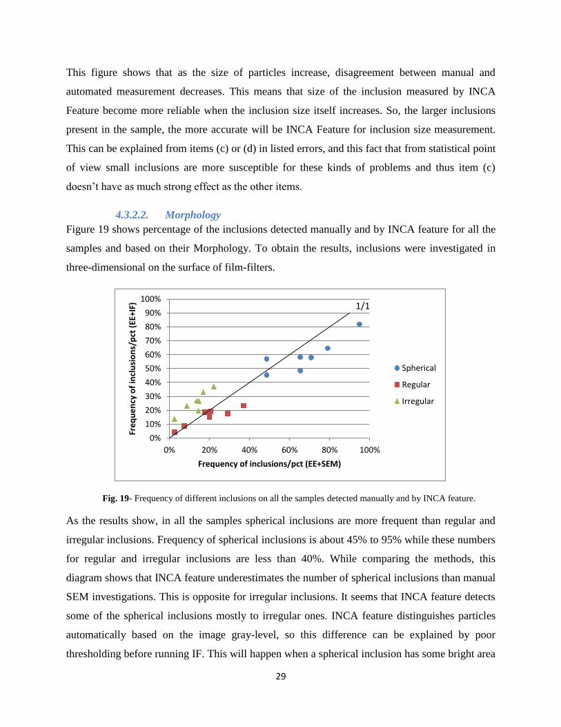
Figure 19 shows percentage of the inclusions detected manually and by INCA feature for all the

samples and based on their Morphology. To obtain the results, inclusions were investigated in

three-dimensional on the surface of film-filters.

Fig. 19- Frequency of different inclusions on all the samples detected manually and by INCA feature.

As the results show, in all the samples spherical inclusions are more frequent than regular and

irregular inclusions. Frequency of spherical inclusions is about 45% to 95% while these numbers

for regular and irregular inclusions are less than 40%. While comparing the methods, this

diagram shows that INCA feature underestimates the number of spherical inclusions than manual

SEM investigations. This is opposite for irregular inclusions. It seems that INCA feature detects

some of the spherical inclusions mostly to irregular ones. INCA feature distinguishes particles

automatically based on the image gray-level, so this difference can be explained by poor

thresholding before running IF. This will happen when a spherical inclusion has some bright area

0%

10%

20%

30%

40%

50%

60%

70%

80%

90%

100%

0% 20% 40% 60% 80% 100%

Fre

qu

en

cy o

f in

clu

sio

ns/

pct

(EE

+IF)

Frequency of inclusions/pct (EE+SEM)

Spherical

Regular

Irregular

1/1

30

around it and the whole bright area is detected as an irregular particle. This can happen when

film filter does not have completely flat surface (Item a) or when there are some bright

precipitations like un-dissolved metal pieces or nitrides around the inclusions (Item b).

As it also can be seen from the diagram, despite the errors that INCA feature has for

distinguishing morphology of the particles, regular inclusions show better detection correlation

than spherical and irregular inclusions.

4.3.2. Comparison of EE+SEM and CS+IF methods

In common metallographic laboratory practice (same as Outokumpu in Avesta), particles and

inclusions are characterized by light optical or scanning electron microscopy of polished planar

micro-sections. By applying digital image analysis (including INCA Feature) on series of

micrographs, the area and from it the volume fraction of these particles can be obtained easily.

However, the conversion of obtained two-dimensional data into true three-dimensional data of

the particles size and numbers plays an important role in quantitative metallography and it can

give us an understanding of the inclusions characteristics and finally improvement of steel

cleanness.

In this section, two-dimensional diameter of inclusions (dA) is converted to spatial diameter of

the inclusions using mean diameter method. Then, calculated size of inclusions is compared with

the size of inclusions which are manually measured through SEM micrographs. Since manual

size measurement of inclusions on the film-filter can be considered as true results, then accuracy

of 2D to 3D conversion can also be investigated for this specific grade of stainless steel.

As mentioned before, for converting 2D size of inclusions into 3D mean diameter method is

used. This method proposed by Fullman for spherical particles and then by DeHoff and Rhines

for other types of particles have been used frequently [16]. The mean spatial diameter of

spherical particles is calculated by the equation (6), which was first derived by Fullman [17]:

�̅�𝑣 = 𝜋

2×�̅�𝐴,𝑖=𝜋

2×

𝑛

∑ (1 𝑑𝐴,𝑖)⁄𝑛𝑖=1

(6)

Where �̅�𝐴(𝐻) is the harmonic mean diameter of particle sections and Aid is the diameter of ith

particle section in a polished cross section and n is the number of particles. Correction factor of

31

/ 2 was obtained from geometric conversion of two-dimensional section and three-dimensional

diameter of a sphere. vd obtained by DeHoff equation is plotted against true values measured

manually through SEM micrographs of the film-filters and presented in figure 20.

Fig. 20- Calculated vd from IF data on polished sections (2D) against true values measured manually through SEM

micrographs on film-filters (3D)

As it can be seen from this figure in all the samples calculated mean spatial diameter of

inclusions from polished sections shows bigger values compared to mean spatial diameters

which is measured manually. Also while comparing these two methods, most of the samples

(more than 72%) show less than 30 percent uncertainty and in total spatial diameter (dv)

calculated by IF/DeHoff shows almost 25 percent overestimation. It can be concluded that by

performing INCA Feature on polished plate samples and then converting the results into three-

dimension, size of the inclusions is overestimated in comparison to the true values but not more

than 30 percent.

If particles on film filter are investigated by running SEM-Feature instead of doing this manually

results will change as shown in figure 21, while the horizontal axis represents INCA-Feature on

film-filter and the vertical axis is the same as the figure 20.

0

0.5

1

1.5

2

2.5

3

3.5

0 0.5 1 1.5 2 2.5

Cal

cula

ted

me

an d

v(I

F/D

eH

off

) (µ

m)

Mean dv (SEM) (µm)

1/1

Δdv=+30

32

Fig. 21- vd obtained by SEM-Feature on plates (2-D) against true values measured by SEM-Feature on film filters

(3-D)

As it can be observed from this figure, results are distributed in the criteria of ±30 error.

However, they show both negative and positive correlation. It should be also mentioned that

results obtained by performing INCA Feature cannot be considered as true values. So, although a

better correlation is observed, more caution should be considered in converting values.

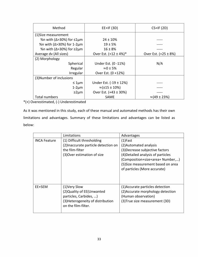
4.4. Final comparison of different methods In this study, automated SEM investigation was done on the film filters and results were

compared with manual SEM measurement which is considered as reference method. The

mechanically polished plate samples were also run by automated SEM and these 2D

measurement results were converted to three-dimensional and then compared with the results of

reference method. Summary of numerical data are listed as below:

0

0.5

1

1.5

2

2.5

3

3.5

0 0.5 1 1.5 2 2.5

Cal

cula

ted

me

an d

v (I

F/D

eH

off

)(µ

m)

Mean dv (INCA) (µm)

Δdv= +30%

1/1

33

Method EE+IF (3D) CS+IF (2D)

(1)Size measurement %n with (Δ>30%) for ≤1µm

%n with (Δ>30%) for 1-2µm %n with (Δ>30%) for ≥2µm

Average dv (All sizes)

24 ± 10% 19 ± 5% 16 ± 8%

Over Est. (+12 ± 4%)*

----- ----- -----

Over Est. (+25 ± 8%)

(2) Morphology Spherical

Regular Irregular

Under Est. (0 -11%)

≈0 ± 5% Over Est. (0 +12%)

N/A

(3)Number of inclusions ≤ 1µm 1-2µm ≥2µm

Total numbers

Under Est. (-19 ± 12%)

≈(±15 ± 10%) Over Est. (+43 ± 30%)

SAME

----- ----- -----

≈(49 ± 23%)

*(+) Overestimated, (-) Underestimated

As it was mentioned in this study, each of these manual and automated methods has their own

limitations and advantages. Summary of these limitations and advantages can be listed as

below:

Limitations Advantages

INCA Feature (1) Difficult thresholding (2)Inaccurate particle detection on the film-filter (3)Over estimation of size

(1)Fast (2)Automated analysis (3)Decrease subjective factors (4)Detailed analysis of particles (Composition+size+area+ Number,…) (5)Size measurement based on area of particles (More accurate)

EE+SEM (1)Very Slow (2)Quality of EE(Unwanted particles, Carbides, …) (3)Heterogeneity of distribution on the film-filter.

(1)Accurate particles detection (2)Accurate morphology detection (Human observation) (3)True size measurement (3D)

34

5. Conclusions 1) Investigations of particle distributions on the gold coated film-filters before and after

transportation show that only less than six percent of the particles misplaced or moved

during transportation. This means that it is possible to transfer gold coated film-filters

with particles after EE to another place for SEM observations. However, this is very

important that samples do not tilt during transportation and severe shaking should also be

avoided.

2) Investigations of particle compositions on film-filter after EE indicate that only 10-20%

of particles are non-metallic oxide inclusions and the rest (80-90%) are some particles

from un-dissolved matrix and inclusions like nitrides, carbides. The interference of these

particles is lower if EE tests are run with 500 coulombs than 1000 coulombs. In this case,

particles separately located on surface of the film-filters and subsequently, error in

automated SEM measurements is significantly smaller.

3) Comparison of EE+IF with reference method (EE+SEM) shows that:

i. Size comparison of the inclusions shows that more than 84 percent of the inclusions

have less than 30 percent disagreement. In total they were overestimated by EE+IF

measurement for about 12±4%. Results also show that by increasing size of the

inclusions disagreement decreases, in which at given magnification EE+IF is an

accurate method for determining size of the inclusions larger than 1µm.

Overestimation of the size can come from some sources, e.g. gray-level non-

uniformity of the film-filter, accumulation of several particles, gray-level gradient in

the particle itself and inappropriate image analysis.

ii. Investigation on morphology of particles show this method has good agreement for

detecting regular particles and that SEM+IF underestimates the number of spherical

inclusions compared to EE+SEM for about 11%. This is opposite for irregular

inclusions for about 12%, while EE+IF identifies some of the spherical inclusions

mostly as irregular. Since automated SEM distinguishes particles based on the image

gray-level, by optimizing SEM parameters like brightness and contrast also by

defining more accurate aspect ratio and circularity factor, disagreement can be

reduced.

35

iii. Number of inclusions per unit volume of steel sample is investigated and compared.

Number of inclusions with the size range of 1-2µm has about 15±10% disagreement.

Number of inclusions larger than 2µm show large overestimation for about 43±10%.

This can be because of few numbers of investigated inclusions in this size range.

Number of inclusions smaller than 1µm is underestimated for about 19±12% which is

due to overestimation of size determination by this method.

4) Investigation on average size (dv) determination of inclusions with CS+IF compared to

EE+SEM show quite high overestimation for about 25±8%. Also total number of

inclusions shows high disagreement compared to reference method. In future work this

disagreement can be reduced by improving SEM parameters and also by using more

accurate method than DeHoff for converting two-dimensional size distribution results to

three-dimensional.

36

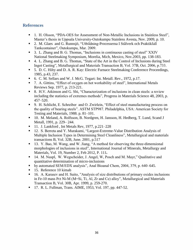
References

1. H. Olsson, “PDA-OES for Assessment of Non-Metallic Inclusions in Stainless Steel”,

Master’s thesis in Uppsala University-Outokumpu Stainless Avesta, Nov. 2009, p. 10.

2. M. Glaes and G. Runnsjö, “Utbildning-Processerna I Stålverk och Praktikfall

Tankcontainer”, Outokumpu, Mar. 2009.

3. L. Zhang and B. G. Thomas, “Inclusions in continuous casting of steel” XXIV

National Steelmaking Symposium, Morelia, Mich, Mexico, Nov.2003, pp. 138-183.

4. L. Zhang and B. G. Thomas, “State of the Art in the Control of Inclusions during Steel

Ingot Casting”, Metallurgical and Materials Transaction B, Vol. 37B, Oct. 2006, p.733.

5. D. C. Hilty and D. A. R. Kay: Electric Furnace Steelmaking Conference Proceedings,

1985, p.43, 237.

6. C. M. Sellars and W. J. McG. Tegart: Int. Metall. Rev., 1972, p.17.

7. A. Gittins, “Effect of oxygen on hot workability of steel”, International Metals

Reviews Sep. 1977, p. 213-221.

8. H.V. Atkinson and G. Shi, “Characterization of inclusions in clean steels: a review

including the statistics of extremes methods”, Progress in Materials Science 48, 2003, p.

457–520.

9. H. Schlicht, E. Schreiber and O. Zwirlein, “Effect of steel manufacturing process on

the quality of bearing steels”. ASTM STP987. Philadelphia, USA: American Society for

Testing and Materials, 1988. p. 81–101.

10. M. Meland, A. Rolfsson, B. Nordgren, H. Jansson, H. Hedberg, T. Lund, Scand J

Metall, 1991, p. 229– 244.

11. J. Lankford , Int Metals Rev, 1977, p.221–228

12. S. Berreta and Y. Murakami, “Largest-Extreme-Value Distribution Analysis of

Multiple Inclusion Types in Determining Steel Cleanliness”, Metallurgical and materials

transactions B, Vol. 32B, June. 2001, p.517

13. Y. Bao, M. Wang, and W. Jiang, “A method for observing the three-dimensional

morphologies of inclusions in steel”, International Journal of Minerals, Metallurgy and

Materials, Vol. 19, Number 2, Feb 2012, P. 111.

14. M. Nuspl, W. Wegscheider, J. Angel, W, Posch and M. Mayr,” Qualitative and

quantitative determination of micro-inclusions

by automated SEM/EDX analysis”, Anal Bioanal Chem, 2004, 379, p. 640–645.

15. Reference 10 kimab

16. A. Karasev and H. Suito, ”Analysis of size distributions of primary oxides inclusions

in Fe-10 mass Pct Ni-M (M=Si, Ti, Al, Zr and Ce) alloy”, Metallurgical and Materials

Transaction B, Vol. 30B, Apr. 1999, p. 259-270.

17. R. L. Fullman, Trans. AIME, 1953, Vol. 197, pp. 447-52.

37

APPENDIXES

Appendix 1.

Ternary diagrams of the samples (A) 405519 (B) 405523 (C) 401931 (D) LDX60505 show different regions where

their oxide inclusions located

A) B)

C) D)