Kirkpatrick, J. P., Wilcox, P. D., & Smith, R. A. (2019). Row-ColumnAddressed Arrays for Nondestructive Evaluation Applications. IEEETransactions on Ultrasonics, Ferroelectrics, and Frequency Control,66(6), 1119-1128. [8681092].https://doi.org/10.1109/TUFFC.2019.2909138

Publisher's PDF, also known as Version of recordLicense (if available):CC BYLink to published version (if available):10.1109/TUFFC.2019.2909138

Link to publication record in Explore Bristol ResearchPDF-document

This is the final published version of the article (version of record). It first appeared online via IEEE athttps://ieeexplore.ieee.org/document/8681092/ . Please refer to any applicable terms of use of the publisher.

University of Bristol - Explore Bristol ResearchGeneral rights

This document is made available in accordance with publisher policies. Please cite only thepublished version using the reference above. Full terms of use are available:http://www.bristol.ac.uk/red/research-policy/pure/user-guides/ebr-terms/

IEEE TRANSACTIONS ON ULTRASONICS, FERROELECTRICS, AND FREQUENCY CONTROL, VOL. 66, NO. 6, JUNE 2019 1119

Row–Column Addressed Arrays for NondestructiveEvaluation Applications

James P. Kirkpatrick , Paul D. Wilcox , and Robert A. Smith

Abstract— Row–column addressed (RCA) arrays are 2-Darrays formed by two orthogonal overlapping linear arraysmade up of elongated elements. This substantially reduces thenumber of elements in the 2-D array. Modeled data are usedto compare RCA arrays in pulse-echo mode to fully populated2-D arrays for nondestructive evaluation (NDE) applicationsand an improved beamforming algorithm based on the totalfocusing method is tested. Improved beamforming has led toa less than half-wavelength diameter conical bottom hole beingsuccessfully detected experimentally using an RCA array, with amaximum signal-to-noise ratio of 17.0 dB (3.s.f). The averagedifference between the −6-dB drop width and the nominaldrill bit diameter when sizing flat bottom holes experimentallyusing RCA arrays is also improved compared to plane B-scanalgorithms from (1.29 ± 0.07) mm to (0.23 ± 0.04) mm. Thesedevelopments demonstrate the advantages of using RCA arraysover conventional fully populated 2-D arrays and provide a basisfor their use, and development, in the field of NDE.

Index Terms— Array signal processing, focusing, imaging,inspection, nondestructive testing, ultrasonic imaging, ultrasonictransducer arrays, ultrasonic transducers.

I. INTRODUCTION

ROW–COLUMN addressed (RCA) arrays, also calledcrossed-electrode transducer arrays [1] or top orthogonal

to bottom electrode arrays [2], are different from fully pop-ulated 2-D arrays in that they are effectively formed by twoorthogonally orientated linear arrays with ne transmit elementsbeing orthogonal to ne receive elements (Fig. 1). RCA arrays,therefore, reduce the number of interconnections, comparedto a fully populated 2-D array, by a factor of 1

2 ne. Thesereductions enable the production of 2-D arrays that wouldcurrently be impossible to manufacture while also reducing theamount of data per frame. Provided the imaging performanceof RCA arrays can match that of fully populated 2-D arrays,their benefits are clear.

RCA arrays were originally invented for use in through-transmission nondestructive evaluation (NDE) in order todecrease the number of elements in 2-D arrays and increase thescanning speed [3]. In addition to continued use in through-transmission NDE [4], [5], these arrays have been used fordifferent applications including particle manipulation [6],

Manuscript received June 4, 2018; accepted March 28, 2019. Date ofpublication April 3, 2019; date of current version June 5, 2019. This workwas supported in part by the Engineering and Physical Sciences ResearchCouncil (EPSRC) through the U.K. Research Centre for Non-DestructiveEvaluation (RCNDE) under Grant EP/L015587/1 and in part by theDefence Science and Technology Laboratory (DSTL). (Corresponding author:James P. Kirkpatrick.)

The authors are with the Department of Mechanical Engineering, Univer-sity of Bristol, Bristol BS8 1TR, U.K. (e-mail: j.kirkpatrick@physics.org;p.wilcox@bristol.ac.uk; robert.smith@bristol.ac.uk).

Digital Object Identifier 10.1109/TUFFC.2019.2909138

photoacoustic imaging [2], and medical imaging [1]. In thesimplest case, image volumes can be formed by using theassumption that each A-scan originates from a fictionalelement located at the intersection between the physicaltransmit and receive elements [Fig. 1(b)] [7]. Recently,a number of developments have been made in the medicalultrasonics field because of increased interest in RCA arrays.Advances in the design of, and imaging using, RCA arrayshave been well summarized in [8], which is currently the mostdefinitive paper on RCA arrays in the medical field. Improvedbeamforming techniques for medical imaging are shown and anew apodization scheme was demonstrated to reduce the edgeeffects of elongated RCA array elements and significantlyincrease the imaging quality to a level comparable with fullypopulated 2-D arrays. Similarly, the field of NDE has madesignificant advances in the past 20 years with the growing useof arrays in the industry as well as the increased adoption ofthe total focusing method (TFM) [10]. Many of these advanceshave come about by the use of systematic approaches, whichcombine modeling and experiment. Array models are oftenused to predict the performance of particular arrays and testpotential improvements, as well as being used to assess imag-ing algorithms in both medical [11] and NDE fields [12], [13].

While advances have been made in both the medical andNDE fields, the use of RCA arrays for NDE has been pre-dominantly limited to through-transmission. However, in 2011,a commercial device which used an RCA array and operatedin pulse-echo mode was produced specifically for NDE. Whilethe device has been introduced into industry, there is a lack ofliterature covering the use of RCA arrays in pulse-echo modefor NDE applications. Wong et al. [7] attempted to use a med-ical RCA array to demonstrate the use of RCA arrays for NDE.This approach, however, was not representative of the state-of-the-art in NDE because of, for example, the size of the array,the use of a medical array, surface scanning, and referencesubtraction. Also, results were shown using images with lowdynamic range. Although the basic imaging algorithms andarrays for medical and NDE fields are similar, the requirementsare often different. These differences include: the importanceof signal-to-coherent and signal-to-random noise, the strengthand quantity of scatterers, and the use of multiple modes.Therefore, with the additional possibility of an NDE specificRCA array, there is a need to review pulse-echo RCA array usefor NDE using current state-of-the-art processes and imagingalgorithms on representative samples.

The organization of this paper is as follows. First,the methodology used to obtain modeled and experimentaldata is introduced. Then, the data processing algorithms

This work is licensed under a Creative Commons Attribution 3.0 License. For more information, see http://creativecommons.org/licenses/by/3.0/

1120 IEEE TRANSACTIONS ON ULTRASONICS, FERROELECTRICS, AND FREQUENCY CONTROL, VOL. 66, NO. 6, JUNE 2019

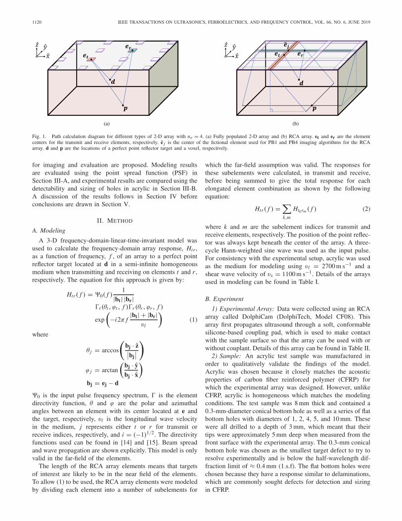
Fig. 1. Path calculation diagram for different types of 2-D array with ne = 4. (a) Fully populated 2-D array and (b) RCA array. et and er are the elementcenters for the transmit and receive elements, respectively. e j is the center of the fictional element used for PB1 and PB4 imaging algorithms for the RCAarray. d and p are the locations of a perfect point reflector target and a voxel, respectively.

for imaging and evaluation are proposed. Modeling resultsare evaluated using the point spread function (PSF) inSection III-A, and experimental results are compared using thedetectability and sizing of holes in acrylic in Section III-B.A discussion of the results follows in Section IV beforeconclusions are drawn in Section V.

II. METHOD

A. Modeling

A 3-D frequency-domain-linear-time-invariant model wasused to calculate the frequency-domain array response, Htr ,as a function of frequency, f , of an array to a perfect pointreflector target located at d in a semi-infinite homogeneousmedium when transmitting and receiving on elements t and r ,respectively. The equation for this approach is given by:

Htr( f ) = �0( f )1

|bt| |br|�t (θt , ϕt , f )�r (θr , ϕr , f )

exp

�−i2π f

|bt| + |br|vl

�(1)

where

θ j = arccos

�bj · z��bj

���

ϕ j = arctan

�bj · ybj · x

�

bj = ej − d

�0 is the input pulse frequency spectrum, � is the elementdirectivity function, θ and ϕ are the polar and azimuthalangles between an element with its center located at e andthe target, respectively, vl is the longitudinal wave velocityin the medium, j represents either t or r for transmit orreceive indices, respectively, and i = (−1)1/2. The directivityfunctions used can be found in [14] and [15]. Beam spreadand wave propagation are shown explicitly. This model is onlyvalid in the far-field of the elements.

The length of the RCA array elements means that targetsof interest are likely to be in the near field of the elements.To allow (1) to be used, the RCA array elements were modeledby dividing each element into a number of subelements for

which the far-field assumption was valid. The responses forthese subelements were calculated, in transmit and receive,before being summed to give the total response for eachelongated element combination as shown by the followingequation:

Htr( f ) =�k,m

Htkrm ( f ) (2)

where k and m are the subelement indices for transmit andreceive elements, respectively. The position of the point reflec-tor was always kept beneath the center of the array. A three-cycle Hann-weighted sine wave was used as the input pulse.For consistency with the experimental setup, acrylic was usedas the medium for modeling using vl = 2700 m s−1 and ashear wave velocity of vs = 1100 m s−1. Details of the arraysused in modeling can be found in Table I.

B. Experiment

1) Experimental Array: Data were collected using an RCAarray called DolphiCam (DolphiTech, Model CF08). Thisarray first propagates ultrasound through a soft, conformablesilicone-based coupling pad, which is used to make contactwith the sample surface so that the array can be used with orwithout couplant. Details of this array can be found in Table II.

2) Sample: An acrylic test sample was manufactured inorder to qualitatively validate the findings of the model.Acrylic was chosen because it closely matches the acousticproperties of carbon fiber reinforced polymer (CFRP) forwhich the experimental array was designed. However, unlikeCFRP, acrylic is homogeneous which matches the modelingconditions. The test sample was 8 mm thick and contained a0.3-mm-diameter conical bottom hole as well as a series of flatbottom holes with diameters of 1, 2, 4, 5, and 10 mm. Thesewere all drilled to a depth of 3 mm, which meant that theirtips were approximately 5 mm deep when measured from thefront surface with the experimental array. The 0.3-mm conicalbottom hole was chosen as the smallest target defect to try toresolve experimentally and is below the half-wavelength dif-fraction limit of ≈ 0.4 mm (1.s.f). The flat bottom holes werechosen because they have a response similar to delaminations,which are commonly sought defects for detection and sizingin CFRP.

KIRKPATRICK et al.: RCA ARRAYS FOR NDE APPLICATIONS 1121

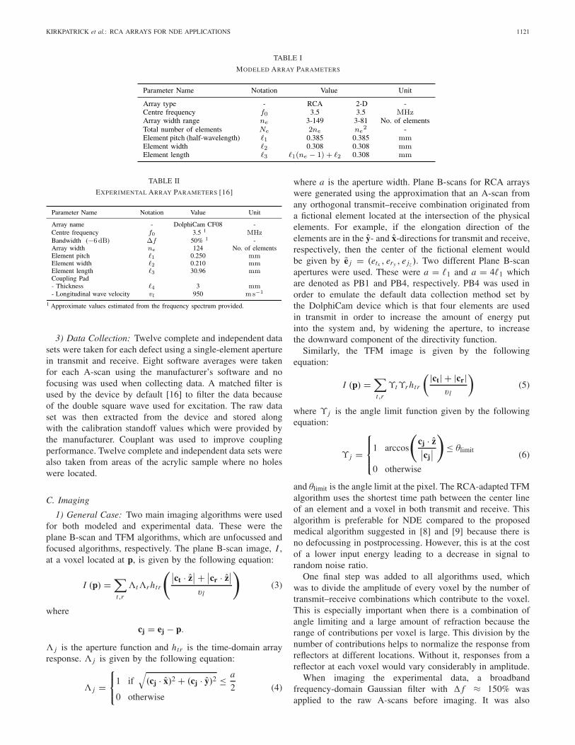
TABLE I

MODELED ARRAY PARAMETERS

TABLE II

EXPERIMENTAL ARRAY PARAMETERS [16]

3) Data Collection: Twelve complete and independent datasets were taken for each defect using a single-element aperturein transmit and receive. Eight software averages were takenfor each A-scan using the manufacturer’s software and nofocusing was used when collecting data. A matched filter isused by the device by default [16] to filter the data becauseof the double square wave used for excitation. The raw dataset was then extracted from the device and stored alongwith the calibration standoff values which were provided bythe manufacturer. Couplant was used to improve couplingperformance. Twelve complete and independent data sets werealso taken from areas of the acrylic sample where no holeswere located.

C. Imaging

1) General Case: Two main imaging algorithms were usedfor both modeled and experimental data. These were theplane B-scan and TFM algorithms, which are unfocussed andfocused algorithms, respectively. The plane B-scan image, I ,at a voxel located at p, is given by the following equation:

I (p) =�t,r

�t�r htr

���ct · z�� + ��cr · z

��vl

�(3)

where

cj = ej − p.

� j is the aperture function and htr is the time-domain arrayresponse. � j is given by the following equation:

� j =⎧⎨⎩

1 if�

(cj · x)2 + (cj · y)2 ≤ a

20 otherwise

(4)

where a is the aperture width. Plane B-scans for RCA arrayswere generated using the approximation that an A-scan fromany orthogonal transmit–receive combination originated froma fictional element located at the intersection of the physicalelements. For example, if the elongation direction of theelements are in the y- and x-directions for transmit and receive,respectively, then the center of the fictional element wouldbe given by e j = (etx , ery , e jz ). Two different Plane B-scanapertures were used. These were a = �1 and a = 4�1 whichare denoted as PB1 and PB4, respectively. PB4 was used inorder to emulate the default data collection method set bythe DolphiCam device which is that four elements are usedin transmit in order to increase the amount of energy putinto the system and, by widening the aperture, to increasethe downward component of the directivity function.

Similarly, the TFM image is given by the followingequation:

I (p) =�t,r

ϒtϒr htr

� |ct| + |cr|vl

�(5)

where ϒ j is the angle limit function given by the followingequation:

ϒ j =

⎧⎪⎨⎪⎩

1 arccos

�cj · z��cj

���

≤ θlimit

0 otherwise

(6)

and θlimit is the angle limit at the pixel. The RCA-adapted TFMalgorithm uses the shortest time path between the center lineof an element and a voxel in both transmit and receive. Thisalgorithm is preferable for NDE compared to the proposedmedical algorithm suggested in [8] and [9] because there isno defocussing in postprocessing. However, this is at the costof a lower input energy leading to a decrease in signal torandom noise ratio.

One final step was added to all algorithms used, whichwas to divide the amplitude of every voxel by the number oftransmit–receive combinations which contribute to the voxel.This is especially important when there is a combination ofangle limiting and a large amount of refraction because therange of contributions per voxel is large. This division by thenumber of contributions helps to normalize the response fromreflectors at different locations. Without it, responses from areflector at each voxel would vary considerably in amplitude.

When imaging the experimental data, a broadbandfrequency-domain Gaussian filter with f ≈ 150% wasapplied to the raw A-scans before imaging. It was also

1122 IEEE TRANSACTIONS ON ULTRASONICS, FERROELECTRICS, AND FREQUENCY CONTROL, VOL. 66, NO. 6, JUNE 2019

assumed, for simplicity, that the array was parallel to theinterface between the coupling pad and the sample in alldirections. In line with this assumption, a single value for thethickness of the coupling pad, averaged across the whole array,was calculated using the highest amplitude reflection withinthe first 50 time points for each A-scan. This coupling padthickness was used in all the path calculations. Modificationswere made to the RCA-adapted TFM algorithm because ofrefraction due to the interface between the coupling pad andthe sample. The interface was discretized and the shortesttime path was calculated by finding the shortest time pathfor each element to interface point to voxel combinationin 2-D. Apart from modifications relating to the coupling pad,data from the DolphiCam device were processed using theimaging algorithms described in (3) and (5). An angle limit ofθlimit = 30◦ was used during all experimental implementationsof the RCA-adapted TFM algorithm. The imaging algorithmswere also applied to the data sets taken on areas of the samplewhich did not contain holes. These images were used toquantify the root-mean-squared (RMS) noise.

2) Simplification and Computational Efficiency: On a reg-ular Cartesian imaging grid, symmetry reduces (5) for RCAarrays to two 2-D path calculations, one in transmit and onein receive, which improves the speed of the algorithm. Bothare calculated using (5) in 2-D as if there were two lineararrays perpendicular in orientation with one in transmit andone in receive. For example, if the elongation direction ofthe elements are in the y- and x-directions for transmit andreceive, respectively, the transmit path calculation would becalculated in the y plane (the plane for which y is the normal)and the receive path calculation in the x plane, as shownschematically in Fig. 1(b). Here, net = ner and n px = n py

symmetry simplifies the problem further and improves thespeed of the algorithm. In this case, only net × n px × n pz

paths need to be calculated. This is substantially less than thenumber of calculations required for full 3-D path calculationsfor every element for fully populated 2-D arrays using theTFM algorithm.

D. Evaluation

1) Point Spread Function Evaluation: The PSF was cal-culated for both types of array and all imaging algorithmsconsidered by applying the imaging algorithms to the modeleddata. The PSF was used to compare the imaging performanceof both fully populated 2-D arrays and RCA arrays andtheir respective imaging algorithms. A decibel scale, nor-malized to the maximum amplitude of the PSF, was used.The imaging performance was quantified using a measure-ment of the −6-dB drop volume of the PSF, V−6 dB, whichwas calculated by summing the number of voxels with anamplitude greater than −6 dB and multiplying it by thevolume of one voxel, Vp . The uncertainty in this value,αV−6 dB , was estimated using the maximum uncertainty inthe volume of a sphere placed in a regular 3-D Cartesiangrid, which was calculated using the relationship between thesurface area and volume of a sphere, yielding an uncertaintyof αV−6 dB = ((9/2)πVpV 2−6 dB)(1/3).

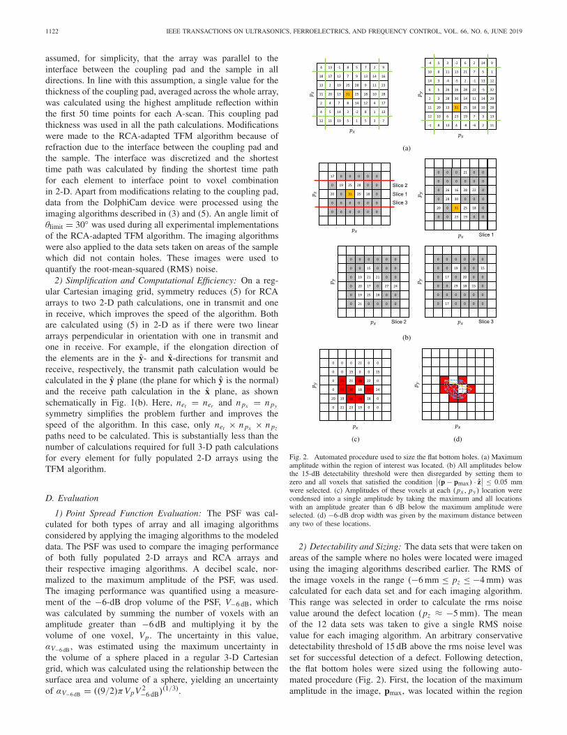
Fig. 2. Automated procedure used to size the flat bottom holes. (a) Maximumamplitude within the region of interest was located. (b) All amplitudes belowthe 15-dB detectability threshold were then disregarded by setting them tozero and all voxels that satisfied the condition

��(p − pmax) · z�� ≤ 0.05 mm

were selected. (c) Amplitudes of these voxels at each (px , py) location werecondensed into a single amplitude by taking the maximum and all locationswith an amplitude greater than 6 dB below the maximum amplitude wereselected. (d) −6-dB drop width was given by the maximum distance betweenany two of these locations.

2) Detectability and Sizing: The data sets that were taken onareas of the sample where no holes were located were imagedusing the imaging algorithms described earlier. The RMS ofthe image voxels in the range (−6 mm ≤ pz ≤ −4 mm) wascalculated for each data set and for each imaging algorithm.This range was selected in order to calculate the rms noisevalue around the defect location (pz ≈ −5 mm). The meanof the 12 data sets was taken to give a single RMS noisevalue for each imaging algorithm. An arbitrary conservativedetectability threshold of 15 dB above the rms noise level wasset for successful detection of a defect. Following detection,the flat bottom holes were sized using the following auto-mated procedure (Fig. 2). First, the location of the maximumamplitude in the image, pmax, was located within the region

KIRKPATRICK et al.: RCA ARRAYS FOR NDE APPLICATIONS 1123

Fig. 3. B-scan images at py = 0 mm of the PSF with a target at d = (0, 0, −5) mm for ne = 41 from modeled data. Fully populated 2-D and RCA arraysare shown from top to bottom, respectively. PB1, PB4, and TFM imaging algorithms are shown from left to right, respectively.

Fig. 4. C-scan images at pz = −5 mm of the PSF with a target at d = (0, 0,−5) mm for ne = 41 from modeled data. Fully populated 2-D and RCA arraysare shown from top to bottom, respectively. PB1, PB4, and TFM imaging algorithms are shown from left to right, respectively.

of interest [Fig. 2(a)]. The region of interest was selectedto be (−13 mm ≤ px ≤ 13 mm), (−13 mm ≤ py ≤13 mm), and (−6 mm ≤ pz ≤ −4 mm). All amplitudesbelow 15 dB were then disregarded by setting them to zerobecause the confidence that they originate from a defect islow. All voxels within the region of interest that satisfied thecondition |(p − pmax) · z| ≤ 0.05 mm were selected in orderto take account of any small deviation in surface height ororientation of the flat bottom hole [Fig. 2(b)]. The amplitudesof these voxels for different pz at each (px , py) location werecondensed into a single amplitude by taking the maximum[Fig. 2(c)]. Following this, all locations with an amplitudegreater than 6 dB below the maximum amplitude were stored[Fig. 2(c)]. Finally, the −6-dB drop width was given by

the maximum distance between any two of these locations[Fig. 2(d)]. This process was repeated for all 12 data sets ofeach defect. The mean was used to give a best estimate of the−6-dB drop width and the standard error was used to quantifythe uncertainty.

III. RESULTS

A. Modeling

Example PSF B- and C-scan images for a target at d =(0, 0,−5) mm for the ne = 41 case for both types of array andall imaging algorithms considered are shown in Figs. 3 and 4,respectively. The images are shown using a decibel scale whichis normalized to the maximum amplitude of the PSF and hasa 40-dB dynamic range. The PSF was calculated for a target

1124 IEEE TRANSACTIONS ON ULTRASONICS, FERROELECTRICS, AND FREQUENCY CONTROL, VOL. 66, NO. 6, JUNE 2019

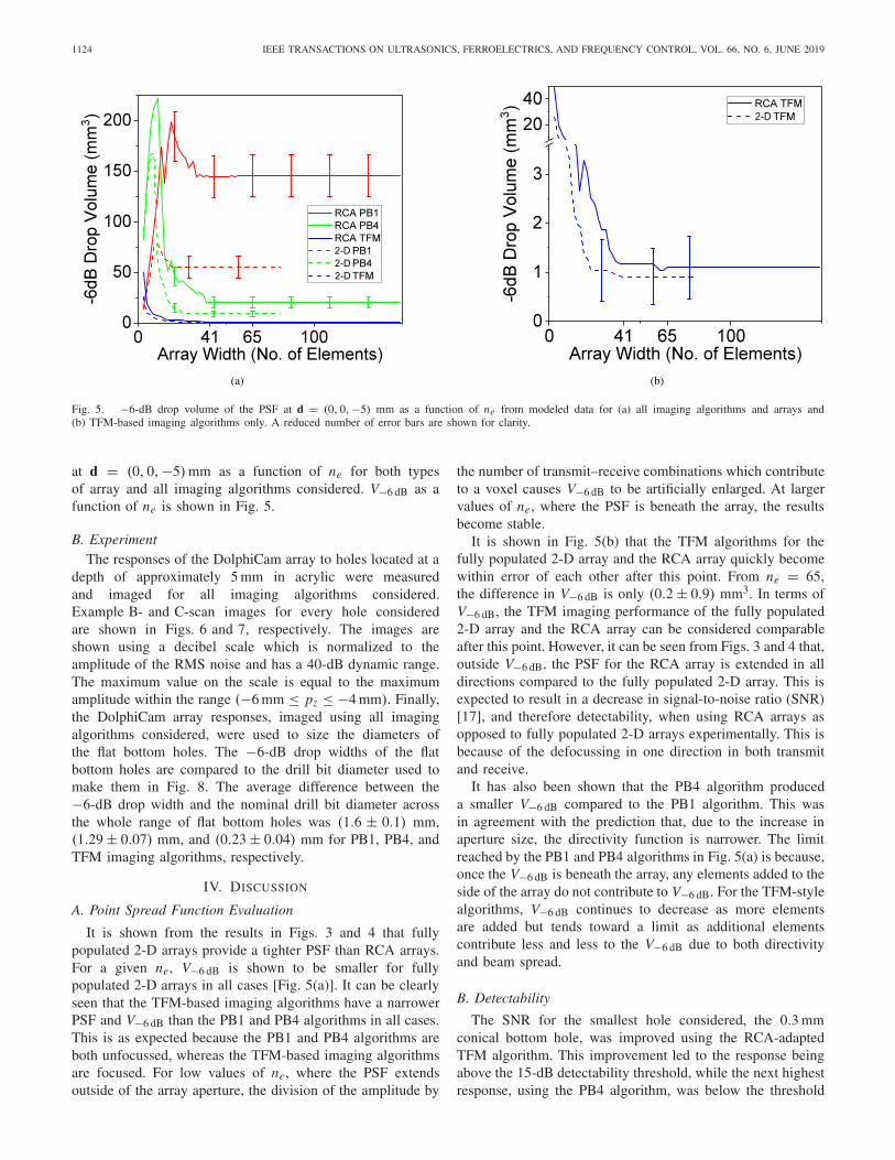
Fig. 5. −6-dB drop volume of the PSF at d = (0, 0,−5) mm as a function of ne from modeled data for (a) all imaging algorithms and arrays and(b) TFM-based imaging algorithms only. A reduced number of error bars are shown for clarity.

at d = (0, 0,−5) mm as a function of ne for both typesof array and all imaging algorithms considered. V−6 dB as afunction of ne is shown in Fig. 5.

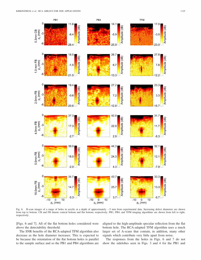
B. ExperimentThe responses of the DolphiCam array to holes located at a

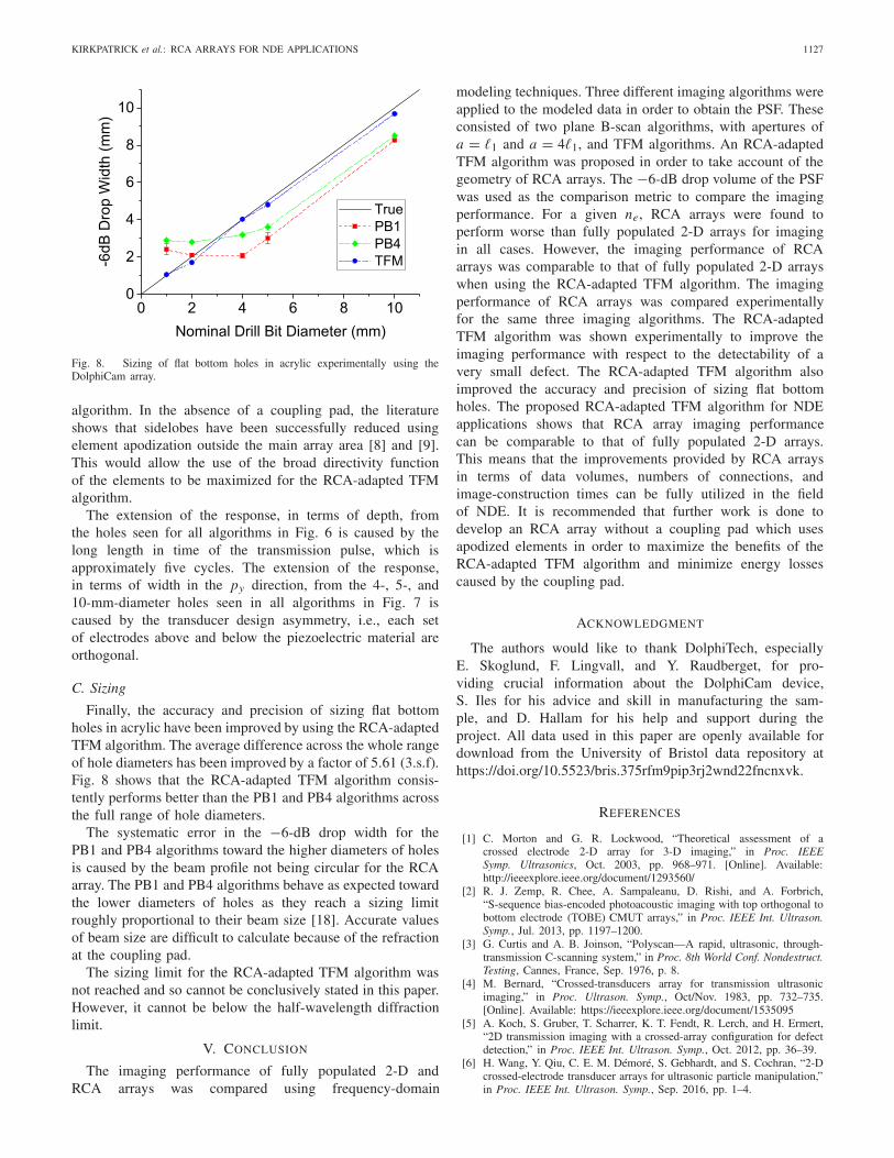
depth of approximately 5 mm in acrylic were measuredand imaged for all imaging algorithms considered.Example B- and C-scan images for every hole consideredare shown in Figs. 6 and 7, respectively. The images areshown using a decibel scale which is normalized to theamplitude of the RMS noise and has a 40-dB dynamic range.The maximum value on the scale is equal to the maximumamplitude within the range (−6 mm ≤ pz ≤ −4 mm). Finally,the DolphiCam array responses, imaged using all imagingalgorithms considered, were used to size the diameters ofthe flat bottom holes. The −6-dB drop widths of the flatbottom holes are compared to the drill bit diameter used tomake them in Fig. 8. The average difference between the−6-dB drop width and the nominal drill bit diameter acrossthe whole range of flat bottom holes was (1.6 ± 0.1) mm,(1.29 ± 0.07) mm, and (0.23 ± 0.04) mm for PB1, PB4, andTFM imaging algorithms, respectively.

IV. DISCUSSION

A. Point Spread Function Evaluation

It is shown from the results in Figs. 3 and 4 that fullypopulated 2-D arrays provide a tighter PSF than RCA arrays.For a given ne, V−6 dB is shown to be smaller for fullypopulated 2-D arrays in all cases [Fig. 5(a)]. It can be clearlyseen that the TFM-based imaging algorithms have a narrowerPSF and V−6 dB than the PB1 and PB4 algorithms in all cases.This is as expected because the PB1 and PB4 algorithms areboth unfocussed, whereas the TFM-based imaging algorithmsare focused. For low values of ne, where the PSF extendsoutside of the array aperture, the division of the amplitude by

the number of transmit–receive combinations which contributeto a voxel causes V−6 dB to be artificially enlarged. At largervalues of ne, where the PSF is beneath the array, the resultsbecome stable.

It is shown in Fig. 5(b) that the TFM algorithms for thefully populated 2-D array and the RCA array quickly becomewithin error of each other after this point. From ne = 65,the difference in V−6 dB is only (0.2 ± 0.9) mm3. In terms ofV−6 dB, the TFM imaging performance of the fully populated2-D array and the RCA array can be considered comparableafter this point. However, it can be seen from Figs. 3 and 4 that,outside V−6 dB, the PSF for the RCA array is extended in alldirections compared to the fully populated 2-D array. This isexpected to result in a decrease in signal-to-noise ratio (SNR)[17], and therefore detectability, when using RCA arrays asopposed to fully populated 2-D arrays experimentally. This isbecause of the defocussing in one direction in both transmitand receive.

It has also been shown that the PB4 algorithm produceda smaller V−6 dB compared to the PB1 algorithm. This wasin agreement with the prediction that, due to the increase inaperture size, the directivity function is narrower. The limitreached by the PB1 and PB4 algorithms in Fig. 5(a) is because,once the V−6 dB is beneath the array, any elements added to theside of the array do not contribute to V−6 dB. For the TFM-stylealgorithms, V−6 dB continues to decrease as more elementsare added but tends toward a limit as additional elementscontribute less and less to the V−6 dB due to both directivityand beam spread.

B. Detectability

The SNR for the smallest hole considered, the 0.3 mmconical bottom hole, was improved using the RCA-adaptedTFM algorithm. This improvement led to the response beingabove the 15-dB detectability threshold, while the next highestresponse, using the PB4 algorithm, was below the threshold

KIRKPATRICK et al.: RCA ARRAYS FOR NDE APPLICATIONS 1125

Fig. 6. B-scan images of a range of holes in acrylic at a depth of approximately −5 mm from experimental data. Increasing defect diameters are shownfrom top to bottom. CB and FB denote conical bottom and flat bottom, respectively. PB1, PB4, and TFM imaging algorithms are shown from left to right,respectively.

[Figs. 6 and 7]. All of the flat bottom holes considered wereabove the detectability threshold.

The SNR benefits of the RCA-adapted TFM algorithm alsodecrease as the hole diameter increases. This is expected tobe because the orientation of the flat bottom holes is parallelto the sample surface and so the PB1 and PB4 algorithms are

aligned to the high-amplitude specular reflection from the flatbottom hole. The RCA-adapted TFM algorithm uses a muchlarger set of A-scans that contain, in addition, many othersignals which contribute very little apart from noise.

The responses from the holes in Figs. 6 and 7 do notshow the sidelobes seen in Figs. 3 and 4 for the PB1 and

1126 IEEE TRANSACTIONS ON ULTRASONICS, FERROELECTRICS, AND FREQUENCY CONTROL, VOL. 66, NO. 6, JUNE 2019

Fig. 7. C-scan images of a range of holes in acrylic at a depth of approximately −5 mm from experimental data. Increasing defect diameters are shownfrom top to bottom. CB and FB denote conical bottom and flat bottom, respectively. PB1, PB4, and TFM imaging algorithms are shown from left to right,respectively.

PB4 algorithms. This is because of the refraction at theinterface between the coupling pad and the sample. At thisinterface, the critical angle θcrit. ≈ 20.6◦ (3.s.f) for longitudinalwaves. Therefore, the coupling pad not only stops the edgewaves propagating into the sample below the center of the

array but also increases the applicability of the intersectionapproximation used for the PB1 and PB4 algorithms by nar-rowing the directivity function in terms of the waves propagat-ing into the sample. The coupling pad also reduces the benefitsof a broad directivity function used by the RCA-adapted TFM

KIRKPATRICK et al.: RCA ARRAYS FOR NDE APPLICATIONS 1127

Fig. 8. Sizing of flat bottom holes in acrylic experimentally using theDolphiCam array.

algorithm. In the absence of a coupling pad, the literatureshows that sidelobes have been successfully reduced usingelement apodization outside the main array area [8] and [9].This would allow the use of the broad directivity functionof the elements to be maximized for the RCA-adapted TFMalgorithm.

The extension of the response, in terms of depth, fromthe holes seen for all algorithms in Fig. 6 is caused by thelong length in time of the transmission pulse, which isapproximately five cycles. The extension of the response,in terms of width in the py direction, from the 4-, 5-, and10-mm-diameter holes seen in all algorithms in Fig. 7 iscaused by the transducer design asymmetry, i.e., each setof electrodes above and below the piezoelectric material areorthogonal.

C. Sizing

Finally, the accuracy and precision of sizing flat bottomholes in acrylic have been improved by using the RCA-adaptedTFM algorithm. The average difference across the whole rangeof hole diameters has been improved by a factor of 5.61 (3.s.f).Fig. 8 shows that the RCA-adapted TFM algorithm consis-tently performs better than the PB1 and PB4 algorithms acrossthe full range of hole diameters.

The systematic error in the −6-dB drop width for thePB1 and PB4 algorithms toward the higher diameters of holesis caused by the beam profile not being circular for the RCAarray. The PB1 and PB4 algorithms behave as expected towardthe lower diameters of holes as they reach a sizing limitroughly proportional to their beam size [18]. Accurate valuesof beam size are difficult to calculate because of the refractionat the coupling pad.

The sizing limit for the RCA-adapted TFM algorithm wasnot reached and so cannot be conclusively stated in this paper.However, it cannot be below the half-wavelength diffractionlimit.

V. CONCLUSION

The imaging performance of fully populated 2-D andRCA arrays was compared using frequency-domain

modeling techniques. Three different imaging algorithms wereapplied to the modeled data in order to obtain the PSF. Theseconsisted of two plane B-scan algorithms, with apertures ofa = �1 and a = 4�1, and TFM algorithms. An RCA-adaptedTFM algorithm was proposed in order to take account of thegeometry of RCA arrays. The −6-dB drop volume of the PSFwas used as the comparison metric to compare the imagingperformance. For a given ne, RCA arrays were found toperform worse than fully populated 2-D arrays for imagingin all cases. However, the imaging performance of RCAarrays was comparable to that of fully populated 2-D arrayswhen using the RCA-adapted TFM algorithm. The imagingperformance of RCA arrays was compared experimentallyfor the same three imaging algorithms. The RCA-adaptedTFM algorithm was shown experimentally to improve theimaging performance with respect to the detectability of avery small defect. The RCA-adapted TFM algorithm alsoimproved the accuracy and precision of sizing flat bottomholes. The proposed RCA-adapted TFM algorithm for NDEapplications shows that RCA array imaging performancecan be comparable to that of fully populated 2-D arrays.This means that the improvements provided by RCA arraysin terms of data volumes, numbers of connections, andimage-construction times can be fully utilized in the fieldof NDE. It is recommended that further work is done todevelop an RCA array without a coupling pad which usesapodized elements in order to maximize the benefits of theRCA-adapted TFM algorithm and minimize energy lossescaused by the coupling pad.

ACKNOWLEDGMENT

The authors would like to thank DolphiTech, especiallyE. Skoglund, F. Lingvall, and Y. Raudberget, for pro-viding crucial information about the DolphiCam device,S. Iles for his advice and skill in manufacturing the sam-ple, and D. Hallam for his help and support during theproject. All data used in this paper are openly available fordownload from the University of Bristol data repository athttps://doi.org/10.5523/bris.375rfm9pip3rj2wnd22fncnxvk.

REFERENCES

[1] C. Morton and G. R. Lockwood, “Theoretical assessment of acrossed electrode 2-D array for 3-D imaging,” in Proc. IEEESymp. Ultrasonics, Oct. 2003, pp. 968–971. [Online]. Available:http://ieeexplore.ieee.org/document/1293560/

[2] R. J. Zemp, R. Chee, A. Sampaleanu, D. Rishi, and A. Forbrich,“S-sequence bias-encoded photoacoustic imaging with top orthogonal tobottom electrode (TOBE) CMUT arrays,” in Proc. IEEE Int. Ultrason.Symp., Jul. 2013, pp. 1197–1200.

[3] G. Curtis and A. B. Joinson, “Polyscan—A rapid, ultrasonic, through-transmission C-scanning system,” in Proc. 8th World Conf. Nondestruct.Testing, Cannes, France, Sep. 1976, p. 8.

[4] M. Bernard, “Crossed-transducers array for transmission ultrasonicimaging,” in Proc. Ultrason. Symp., Oct/Nov. 1983, pp. 732–735.[Online]. Available: https://ieeexplore.ieee.org/document/1535095

[5] A. Koch, S. Gruber, T. Scharrer, K. T. Fendt, R. Lerch, and H. Ermert,“2D transmission imaging with a crossed-array configuration for defectdetection,” in Proc. IEEE Int. Ultrason. Symp., Oct. 2012, pp. 36–39.

[6] H. Wang, Y. Qiu, C. E. M. Démoré, S. Gebhardt, and S. Cochran, “2-Dcrossed-electrode transducer arrays for ultrasonic particle manipulation,”in Proc. IEEE Int. Ultrason. Symp., Sep. 2016, pp. 1–4.

1128 IEEE TRANSACTIONS ON ULTRASONICS, FERROELECTRICS, AND FREQUENCY CONTROL, VOL. 66, NO. 6, JUNE 2019

[7] L. L. P. Wong, A. I. H. Chen, Z. Li, A. S. Logan, and J. T. W. Yeow,“A row–column addressed micromachined ultrasonic transducer arrayfor surface scanning applications,” Ultrasonics, vol. 54, no. 8,pp. 2072–2080, Dec. 2014. doi: 10.1016/j.ultras.2014.07.002.

[8] M. F. Rasmussen, T. L. Christiansen, E. V. Thomsen, and J. A. Jensen,“3-D imaging using row-column-addressed arrays with integratedapodization—Part I: Apodization design and line element beamforming,”IEEE Trans. Ultrason., Ferroelectr., Freq. Control, vol. 62, no. 5,pp. 947–958, May 2015.

[9] T. L. Christiansen, M. F. Rasmussen, J. P. Bagge, L. N. Moesner,J. A. Jensen, and E. V. Thomsen, “3-D imaging using row–column-addressed arrays with integrated apodization—Part II: Transducer fab-rication and experimental results,” IEEE Trans. Ultrason., Ferroelectr.,Freq. Control, vol. 62, no. 5, pp. 959–971, May 2015.

[10] C. Holmes, B. W. Drinkwater, and P. D. Wilcox, “Post-processing of thefull matrix of ultrasonic transmit-receive array data for non-destructiveevaluation,” NDT & E Int., vol. 38, no. 8, pp. 701–711, Dec. 2005.doi: 10.1016/j.ndteint.2005.04.002.

[11] C. E. M. Demore, A. W. Joyce, K. Wall, and G. R. Lockwood,“Real-time volume imaging using a crossed electrode array,” IEEETrans. Ultrason., Ferroelectr., Freq. Control, vol. 56, no. 6,pp. 1252–1261, Jun. 2009.

[12] B. W. Drinkwater and P. D. Wilcox, “Ultrasonic arrays for non-destructive evaluation: A review,” NDT & E Int., vol. 39, no. 7,pp. 525–541, Oct. 2006.

[13] J. Zhang, B. W. Drinkwater, P. D. Wilcox, and A. J. Hunter,“Defect detection using ultrasonic arrays: The multi-mode total focusingmethod,” NDT & E Int., vol. 43, no. 2, pp. 123–133, Mar. 2010.doi: 10.1016/j.ndteint.2009.10.001.

[14] S.-C. Wooh and Y. Shi, “Three-dimensional beam directivity ofphase-steered ultrasound,” J. Acoust. Soc. Amer., vol. 105, no. 6,pp. 3275–3282, Jun. 1999. doi: 10.1121/1.424655.

[15] G. F. Miller and H. Pursey, “The field and radiation impedance ofmechanical radiators on the free surface of a semi-infinite isotropicsolid,” Proc. Roy. Soc. London A, Math. Phys. Eng. Sci., vol. 223,no. 1155, pp. 521–541, May 1954.

[16] F. Lingvall and E. Skoglund, DolphiCam 1.3 Technical Paper. Dol-phiTech, 2015.

[17] P. D. Wilcox, “Array imaging of noisy materials,” AIP Conf., vol. 1335,no. 1 pp. 890–897, Jun. 2011.

[18] R. A. Smith, “Ultrasonic defect sizing in carbon-fibre composites: Aninitial study,” Insight, vol. 36, no. 8, pp. 595–605, 1994.

James P. Kirkpatrick was born in the U.K.He received the B.Sc. degree (Hons.) in physics fromthe University of Warwick, Coventry, U.K., in 2015.He is currently pursuing the Eng.D. degree with theUniversity of Bristol, Bristol, U.K., and also withthe Defence Science and Technology Laboratory,Salisbury, U.K.

His research interests include novel array trans-ducer designs, laser ultrasonics, and ultrasonic dif-fuse fields.

Paul D. Wilcox was born in Nottingham, U.K.,in 1971. He received the M.Eng. degree in engineer-ing science from the University of Oxford, Oxford,U.K., in 1994 and the Ph.D. degree from ImperialCollege London, London, U.K., in 1998.

He remained in the Non-Destructive Test-ing (NDT) Research Group, Imperial College Lon-don, as a Research Associate until 2002, working onthe development of guided wave array transducersfor large area inspection. Since 2002, he has beenwith the Department of Mechanical Engineering,

University of Bristol, Bristol, U.K., where his current title is Professor ofdynamics. He held an EPSRC Advanced Research Fellowship in quantitativestructural health monitoring from 2007 to 2012 and was Head of theMechanical Engineering Department, University of Bristol, from 2015 to2018. In 2015, he was a Co-Founder of Inductosense Ltd., Bristol, a spin-outcompany which is commercializing inductively coupled embedded ultrasonicsensors. His research interests include array transducers, embedded sensors,ultrasonic particle manipulation, long-range guided wave inspection, structuralhealth monitoring, elastodynamic scattering, and signal processing.

Robert A. Smith received the B.A. degreein physics from the University of Cambridge,Cambridge, U.K., in 1983, the M.Sc. degree appliedacoustics from the Kings College, London, U.K.,in 1986, and the Ph.D. degree from the Universityof Nottingham, Nottingham, U.K., in 2010, witha focus on the ultrasonic 3-D characterization offiber-reinforced composites.

He is currently a Professor of nondestructivetesting (NDT) and high value manufacturing withthe University of Bristol, Bristol, U.K. He spent

six years at the National Physical Laboratory and then moved to theNon-Destructive Evaluation (NDE) Group, Royal Aerospace Establishment(RAE), Farnborough, U.K., in 1989. After several years as the Fellow in NDEat RAE, the Defence Evaluation and Research Agency (DERA), Farnborough,U.K., and then QinetiQ Ltd., Farnborough, he became a QinetiQ Senior Fellowin 2011. He moved to the University of Bristol in 2013 to accept a personalchair and commence a five-year EPSRC Fellowship in manufacturing. In 2018,he became the Director of the U.K. Research Centre for Non-DestructiveEvaluation (RCNDE). He has authored more than 120 publications, for whichhe was awarded the John Grimwade Medal five times and the Roy SharpePrize for 1996 by the British Institute of NDT, of which he is an HonoraryFellow and was the President from 2015 to 2016. He is also a fellow of theInstitute of Physics, a Chartered Physicist, and a Chartered Engineer.