Roughness during border irrigation

Item Type text; Thesis-Reproduction (electronic)

Authors Roth, Robert Leroy, 1943-

Publisher The University of Arizona.

Rights Copyright © is held by the author. Digital access to this materialis made possible by the University Libraries, University of Arizona.Further transmission, reproduction or presentation (such aspublic display or performance) of protected items is prohibitedexcept with permission of the author.

Download date 06/07/2018 12:06:56

Link to Item http://hdl.handle.net/10150/566355

ROUGHNESS DURING BORDER IRRIGATION

byRobert Leroy Roth

A Thesis Submitted to the Faculty of the

DEPARTMENT OF AGRICULTURAL ENGINEERING

In Partial Fulfillment of the Requirements For the Degree of

MASTER OF SCIENCE

In the Graduate College

THE UNIVERSITY OF ARIZONA

1 9 7 1

STATEMENT BY AUTHOR

This thesis has been submitted in partial fulfillment of re­quirements for an advanced degree at The University of Arizona and is deposited in the University Library to be made available to borrowers under rules of the Library.

Brief quotations from this thesis are allowable without specialpermission, provided that accurate acknowledgment of source is made. Requests for permission for extended quotation from or reproduction of this manuscript in whole or in part may be granted by the head of the major department or the Dean of the Graduate College when in his judg­ment the proposed use of the material is in the interests of scholar­ship. In all other instances, however, permission must be obtained from the author.

SIGNED:

APPROVAL BY THESIS DIRECTOR

This thesis has been approved on the date shown below:

GMEIERAssociate Professor of Agricultural Engineering

ACKNOWLEDGMENTS

The author wishes to express sincere thanks to the Agricul­

tural Engineering Department, University of Arizona for the oppor­

tunity of conducting this research. Fiscal support for this project

was provided by the Arizona Agricultural Experiment Station as part

of the Western Regional Research Project W-65.

Special thanks are expressed for the guidance and advice given

by Dr. Delxnar Fangmeier, who served as advisor for this study.

Special thanks are also expressed to Mr. David W. Fonken, who spent

many long hours in helping with this project. Thanks are also due to

Agricultural Engineering Departmental personnel, who helped in build­

ing the equipment necessary for this study, the collection of field

data, and making innumerable roughness measurements of the soil sur­face castings.

ill

TABLE OF CONTENTS

LIST OF TABLES............................................. vi

LIST OF ILLUSTRATIONS..................................... ix

ABSTRACT ................................................... x

1. INTRODUCTION ............................................... 12. LITERATURE R E V I E W .................. 3

Roughness Coefficients .................................Roughness Coefficients from Empirical Equations . . Roughness Factors from Logarithmic Equations . . . . Roughness Parameter from Logarithmic Equation . . . 10

Infiltration . . . . . . . . . . . ..................... 15

3. EQUIPMENT AND PROCEDURE................................... 17Equipment.............................. 17

Delivery S y s t e m ................................... 17Runoff S y s t e m .................... 17Precision Field Border ............................. 18Floats and Recorders.............................. 19Soil Profile Probe ................................. 22

Procedure................ 26Border Preparation ................................. 26Irrigation Procedure ............................... 31Post-Irrigation Procedure .............. . . . . . 32

4. BORDER FLOW ANALYSIS....................................... 34

S l o p e ............ . 34Flow Depth............................................. 36Hydraulic Radius ....................................... 37Average Velocity................................ 37Roughness Coefficients ................................ 42

5. PRESENTATION OF D A T A ....................................... 44

Measured Flow Depths .................... . . . . . . . 46Computed Velocities ................................... 49Water Surface Slopes.................... 49

Page

iv

on on co

V

Page

Determination of Flow Regime........................... 53Roughness Coefficients and Parameters ............ • . 5^Advance and Recession ................................. 55

6 . DISCUSSION AND CONCLUSIONS................ 60

Discussion . . . . . . . ............................... 60Roughness................................ 60Effects of Parameters ............................. 7^

Conclusions ..................................... .. . . 77

APPENDIX A: DETERMINATION OF FLOW REGIME ................ 79

APPENDIX B: COMPUTED VALUES OF MANNING, SAYRE-ALBERTSCN, CHEZY, AND DARCY-WEISBACHROUGHNESSES AND MEASURED X VALUES . . . . . . 84

LIST OF SYMBOLS ............................................ 94

TABLE OF CONTENTS— Continued

LIST OF REFERENCES 97

LIST OF TABLES

1. Values of Device Calibration Constants Usedin Equation ..................................... .. 23

2. Summary of Data for Irrigations 8, 9* 10, and 1 1 ........ 45

3. Measured Flow Depths for Irrigation 8 ................... 47

4. Measured Flow Depths for Irrigation 9 ............ 4?

5. Measured Flow Depths for Irrigation 1 0 ................... 48

6. Measured Flow Depths for Irrigation 1 1 ................... 48

7. Computed Velocities for Irrigation 8 . . . . ............. 50

8. Computed Velocities for Irrigation 9 • • ................. 50

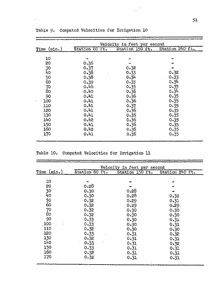
9. Computed Velocities for Irrigation 10 ................... 51

10. Computed Velocities for Irrigation 11 ................... 51

11. Water Surface Slopes for Irrigations 8, 9# 10, and 11 . . 52

12. Advance and Recession Times for Irrigation 8 ............ 57

13. Advance and Recession Times for Irrigation 9 ............ 57

14. Advance and Recession Times for Irrigation 1 0 .......... 58

15. Advance and Recession Times for Irrigation 1 1 .......... 58

16. Advance and Recession Equations for Irrigations 8,9, 10, and 1 1 .................. .................... 59

17. Summary of Data for Irrigations 1 through 7 ............ 69

18. Roughness Changes Due to a Flow Depth E r r o r ............. 78

19. Roughness Changes Due to Slope Errors ................... 78

20. Average Reynolds Number for Irrigation 8 ................. 80

21. Average Reynolds Number for Irrigation 9 ................. 80

Table Page

vi

Table Page

22. Average Reynolds Number for Irrigation 10 .............. 8l

23. Average Reynolds Number for Irrigation 1 1 .......... .. . 8l

24. Boundary Condition Values for Irrigation 8 . . . . . . . 82

25• Boundary Condition Values for Irrigation 9 8226. Boundary Condition Values for Irrigation 1 0 ........ .. . 83

27. Boundary Condition Values for Irrigation 11 ............ 83

28. Computed Values of Manning’s n for Irrigation 8 . . . . 85

2 9. Computed Values of Manning's n for Irrigation 9 • • • • 85

30. Computed Values of Manning's n for Irrigation 10 . . . 86

31. Computed Values of Manning's n for Irrigation 11 . . . 86

32. Computed Values of Sayre-Albertscn's Xfor Irrigation 8 .................. . . . . . . . . 87

33 • Computed Values of Sayre-Albertson's Xfor Irrigation 9 .................................... 87

34. Computed Values of Sayre-Albertson's Xfor Irrigation 1 0 ....................... 88

35• Computed Values of Sayre-Albertson's Xfor Irrigation 11 . ................................. 88

36. Computed Values of Chezy's C for Irrigation 8 .... 89

37• Computed Values of Chezy's C for Irrigation 9 .... 89

38. Computed Values of Chezy's C for Irrigation 10 . . . . 90

39* Computed Values of Chezy's C for Irrigation 11 . . . . 90

40. Computed Values of Darcy-Weisbach's ffor Irrigation 8 .................................... 91

41. Computed Values of Darcy-Weisbach's ffor Irrigation 9 .................................... 91

viiLIST OF TABLES— Continued

viii

Table Page

42. Computed Values of Darcy-Weisbach‘s ffor Irrigation 1 0 ...................................

43. Computed Values of Darcy-Weisbach * s ffor Irrigation 11 . . . ......................... .. . 92

44. Values of Sayre-Albertson's X from Soil Casts . . . . . 93

LIST OF TABLES— Continued

LIST OF ILLUSTRATIONS

Figure Page

1. Free Body Diagram of Uniform Open Channel F l o w .......... 7

2. Float-Actuated Potentiometer for MeasuringWater Surface Elevations........................... • 20

3. Circuit Diagram for Measuring Devices .................... 21

4. Calibration Curve for Water SurfaceElevation Float 3 .......................... 24

5. Soil Roughness Probe Ready to Read a Soil C a s t ....... 25

6. Land Preparation Prior to Each Irrigation ............... 27

7« Schematic for Determining Border Elevation Control . . . . 29

8. Longitudinal Cross Section of Border Irrigationduring Advance ....................................... 40

9. Soil Castings of Station 8 for Irrigation 1 0 .............. 56

10. Variation of Manning’s n and Sayre-Albertson's %during Irrigation 8 ................................. 6l

11. Variation of Manning’s n and Sayre-Albertson’s %during Irrigation 9 .................. 62

12. Variation of Manning’s n and Sayre-Albertson * s Xduring Irrigation 10 ................................. 63

13• Variation of Manning’s n and Sayre-Albertson’s %during Irrigation 1 1 ................................ 64

14. Measured Sayre-Albertson’s X from BEFORE Castings . . . 70

15. Measured Sayre-Albertson’s X from AFTER Castings . . . . 71

16. Average Sayre-Albertson*s X from BEFORE andAFTER Castings....................................... 73

ix

ABSTRACT

Four irrigations were made at a fixed slope on a 300-foot

precision field border to determine variation in resistance of flow

in time (during the irrigation) and space (along the border) on a

bare soil surface. Measurements were made to obtain the border in­

flow, outflow, and flow depth hydrographs. A volume balance analysis

of the flow during the irrigation was made at different time intervals

and reaches along the border. After the volume balance was completed,

average velocities at these time intervals and reaches were computed.

Steady, uniform flow equations were employed to compute

roughness coefficients during the time intervals and at different

reaches to determine the resistance of flow. Roughness was also

determined by physical measurements on plaster castings of the soil

surface at selected stations.

Results from the four irrigations show no pattern of roughness

variation in time or space. Measured and computed time of advance and

recession and computed infiltration equations are also presented.

x

CHAPTER 1

INTRODUCTION

Border irrigation is a procedure for adding water to the soil

to increase soil moisture. The water flows over a porous bed, thus,

the flow conditions are usually unsteady and nonuniform.

To study border irrigation, the recognition and understanding

of hydraulic variables are essential. The pertinent variables as

listed by Israelson and Hansen (7) are: l) size of the application

stream, 2 ) rates of advance and recession, 3 ) length of the border,

4 ) depth of flow, 5) infiltration, 6 ) slope, 7 ) soil or vegetative

resistance, 8 ) erosion hazard, 9) shape of the flow channel, 10)

desired soil moisture to be added, and 11) fluid characteristics.

The objective of this study was to determine how resistance

to flow varies in time (during the irrigation) and space (along the

border) on the bare soil surface of an irrigation border. Also this

study was conducted to provide data on border irrigation variables for

calibrating mathematical models which simulate border irrigation.

To compute the resistance to flow, steady, uniform flow equa­

tions were employed. The measurement or computation of slope, flow

depth, hydraulic radius, and average velocity were required to calcu­

late roughness coefficients or roughness parameters. Herein rough­

ness coefficient and roughness parameter will be used synonymously to

1

2describe a resistance to flow. Also a statistical soil roughness

measurement was used to compare with computed roughness parameters.

Even though the flew conditions during border irrigation are

unsteady and nonuniform, the steady, uniform flow equations were used

because they are used by designers, and no other simple equations

exist at this time. It will be shown in a later chapter that after the

water had advanced the length of the border, the slopes of the channel

bed, water surface, and total energy line are approximately identical,

indicating that the steady, uniform flow equations can be applied

during border irrigation.

The variables, slope, size of the application stream, and

length and width of the border were held constant for each irrigation

test. The size of the application stream was kept constant for each

irrigation test but did vary between tests. As a result of the mea­

surements made, it was also possible to determine infiltration and therates of advance and recession

CHAPTER 2

LITERATURE REVIEW

Extensive research has been done on roughness coefficients

and infiltration. However, only those articles which relate to this

study will be reviewed.

Roughness Coefficients

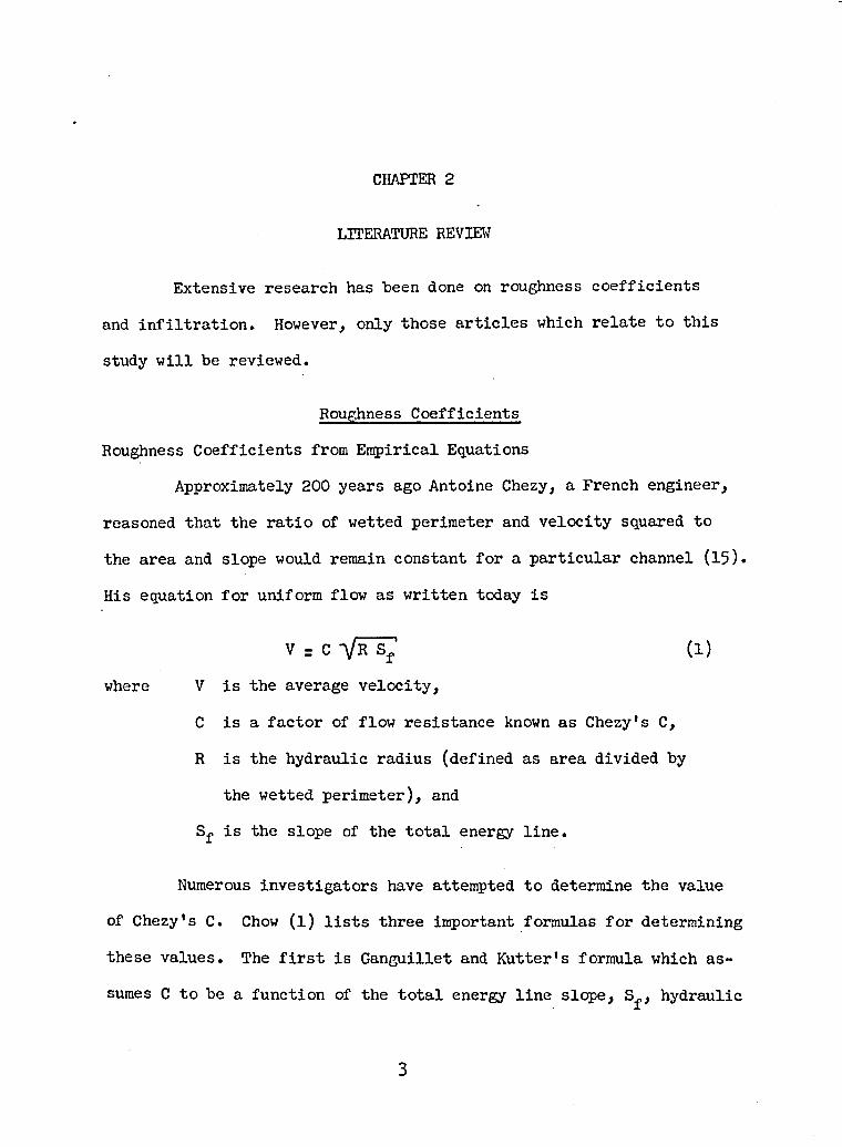
Roughness Coefficients from Empirical Equations

Approximately 200 years ago Antoine Chezy, a French engineer,

reasoned that the ratio of wetted perimeter and velocity squared to

the area and slope would remain constant for a particular channel (15)•

His equation for uniform flow as written today is

V = C V R sf (1)where V is the average velocity,

C is a factor of flow resistance known as Chezy's C,

R is the hydraulic radius (defined as area divided by

the wetted perimeter), and

Sf is the slope of the total energy line.

Numerous investigators have attempted to determine the value

of Chezy * s C. Chow (l) lists three important formulas for determining

these values. The first is Ganguillet and Kutter's formula which as­

sumes C to be a function of the total energy line slope, S^, hydraulic

3

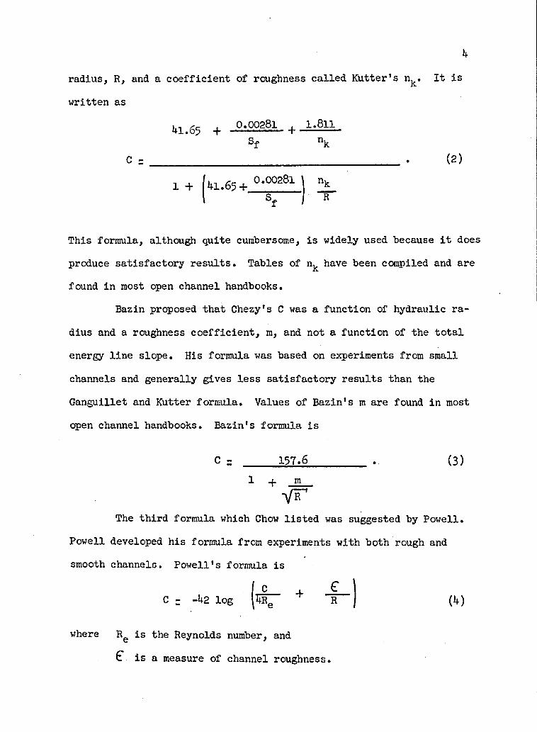
It is

4

radius, R, and a coefficient of roughness called Rutter's n^.

written as

41.65 + _0:00g8l. + J ^ l lSf nk

1 + 41.6S+ 0 -00281

(2)

This formula, although quite cumbersome, is widely used because it does

produce satisfactory results. Tables of nk have been compiled and are

found in most open channel handbooks.

Bazin proposed that Chezy's C was a function of hydraulic ra­

dius and a roughness coefficient, m, and not a function of the total

energy line slope. His formula was based on experiments from small

channels and generally gives less satisfactory results than the

Ganguillet and Rutter formula. Values of Bazin's m are found in most

open channel handbooks. Bazin's formula is

C = 157.6__________ . (3)1 m

y r

The third formula which Chow listed was suggested by Powell.

Powell developed his formula from experiments with both rough and

smooth channels. Powell's formula is

C - -42 log + cR (4)

where Re is the Reynolds number, and

€ is a measure of channel roughness

5In very turbulent flow (high Reynolds number) the first term of the

logarithmic expression becomes negligible and for smooth channels £ becomes very small and the last term becomes negligible. The practical

application of this formula is limited because more determinations of

the value € , channel roughness, are needed.

The Darcy-Weisbach equation, usually applied to pipe flow, can

be used for uniform open channel flow. Their equation is

8 g R S-f (5)

f

where f is the friction factor and

g is the acceleration due to gravity.

The ASCE Task Force on Friction Factors in Open Channels (17), recom­

mends the use of the Darcy-Weisbach friction factor, f, since it is

better correlated to a wider range of conditions than other roughness

coefficients.

Many engineers use the Manning equation for uniform flow be­

cause of its simplicity and the satisfactory results obtained.

Manning’s equation is

V = 1.486 R2/ 3 Sf1/ 2 (6 )n

where n is a roughness coefficient commonly called Manning’s n.

Manning's n is normally assumed to be a constant for a channel but

various investigations have shown it to be dependent on surface rough­

ness, channel alignment, irregularity, shape, and size, vegetative

cover, discharge, and depth of flow.

6

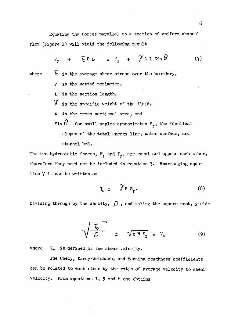
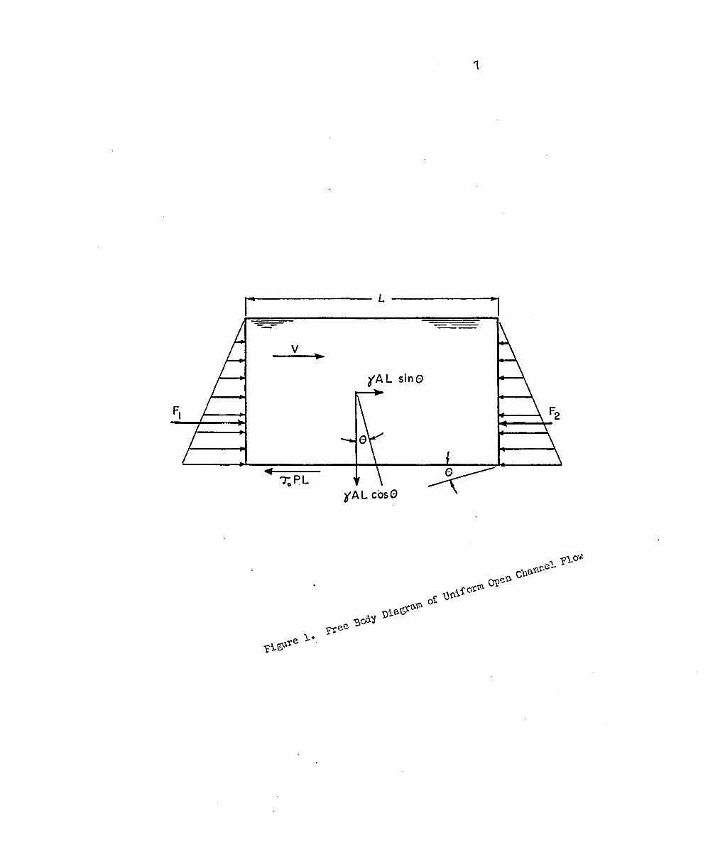
Equating the forces parallel to a section of uniform channel

flow (Figure l) will yield the following result

F2 + L = F1 -f / A L Sin 0 (?)

where %> is the average shear stress over the boundary,

P is the wetted perimeter,V

L is the section length,

'f is the specific weight of the fluid,

A is the cross sectional area, and

Sin Q for small angles approximates S^, the identical

slopes of the total energy line, water surface, and

channel bed.

The two hydrostatic forces, F^ and F^, are equal and oppose each other,

therefore they need not be included in equation 7* Rearranging equa­

tion 7 it can be written as

% z Sf. (8 )

Dividing through by the density, p , and taking the square root, yields

V s R sf' - v* (9)

where V* is defined as the shear velocity.

The Chezy, Darcy-Weisbach, and Manning roughness coefficients

can be related to each other by the ratio of average velocity to shear

velocity. From equations 1, 5 and 6 one obtains

1

L

/ A L sin0

ftee •PicAV

8

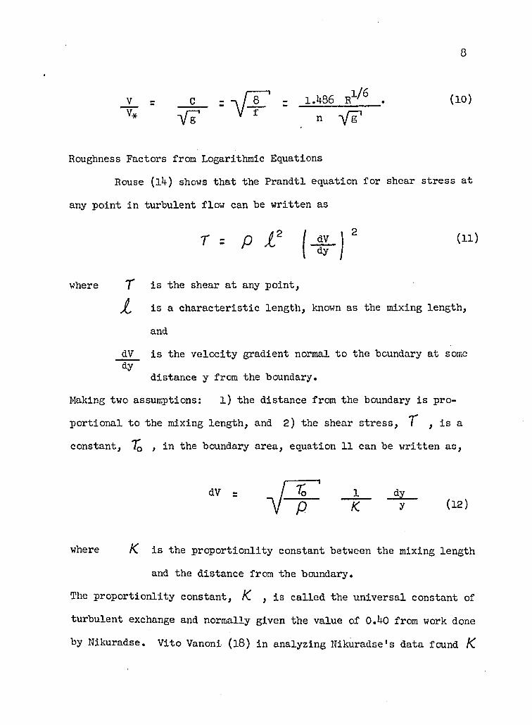
V 5 c - -. / 8 - 1.486 R1/6 . (10)

V* VT V f n V F 1

Roughness Factors from Logarithmic EquationsRouse (l4) shows that the Prandtl equation for shear stress at

any point in turbulent flow can be written as

r r p X 2 | _dV_| 2 (11)

where T is the shear at any point,is a characteristic length, known as the mixing length,

anddV is the velocity gradient normal to the boundary at some dy

distance y from the boundary.

Making two assumptions: l) the distance from the boundary is pro­

portional to the mixing length, and 2 ) the shear stress, T , is a

constant, in the boundary area, equation 11 can be written as,

dV % _1 dyK y (12)

where K is the proportionlity constant between the mixing length

and the distance from the boundary.

The proportionlity constant, K , is called the universal constant of

turbulent exchange and normally given the value of 0.40 from work done

by Nikuradse. Vito Vanoni (l8 ) in analyzing Nikuradse’s data found K

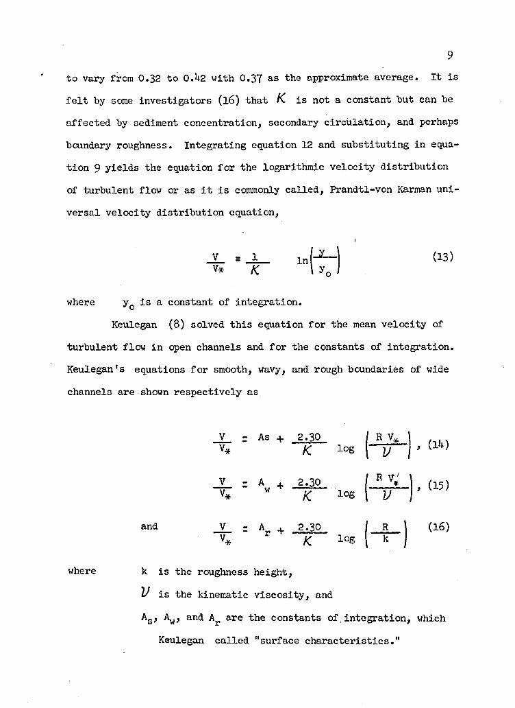
9to vary from 0.32 to 0.42 with 0.37 as the approximate average. It is

felt by some investigators (l6 ) that K is not a constant but can be

affected by sediment concentration, secondary circulation, and perhaps

boundary roughness. Integrating equation 12 and substituting in equa­

tion 9 yields the equation for the logarithmic velocity distribution

of turbulent flow or as it is commonly called, Prandtl-von Karman uni­

versal velocity distribution equation,

= J Lv* % In y (13)

where yQ is a constant of integration.

Keulegan (8) solved this equation for the mean velocity of

turbulent flow in open channels and for the constants of integration.

Keulegan*s equations for smooth, wavy, and rough boundaries of wide

channels are shown respectively as

where

V - As + 2.30 ( R M , (14)V* K log V 1V = A + 2.30 ' R v* ' , (15)V* w K log v ]V = A 2 .30 R (16)V*

iK log k

k is the roughness height,

V is the kinematic viscosity, andAg, Ay, and Ar are the constants of.integration, which

Keulegan called "surface characteristics."

Chow (l) states that these constants not only include the channel

shape function but also such uncertain factors as the effect of free

surface and the effect of nonuniform distribution of the tractive

force at the boundary.

Roughness Parameter from Logarithmic Equation

Sayre and Albertson (l6 ) reviewing Keulegan’s equation for

rough boundaries (equation 16) concluded that since k is a measure of

roughness height, must be a factor dependent on the shape and ar­

rangement of the roughness elements. They combined A with k into a

single roughness parameter, X , to form the equation

10

V_ = 2.30 f dV* K l0S l X

(17)

where X is a single roughness parameter that is dependent on

size, shape, and spacing of roughness elements, and

d is the depth of flow occurring when the slopes of the

energy gradient, water surface, and channel bed are

all equal.

Depth of flow, d, which has replaced hydraulic radius, R, is for wide

channels approximately equal to hydraulic radius.

Their analysis is based on two assumptions: l) the flow is

hydrodynamically rough (viscosity has a negligible effect), and 2 )

the channel is wide or bed roughness is much larger than the side wall

roughness so that side wall effects are appreciably reduced. Sayre

and Albertson found that equation 17 best fit their data when the uni­

versal constant for turbulent exchange, K. , was equal to 0 .38. Over

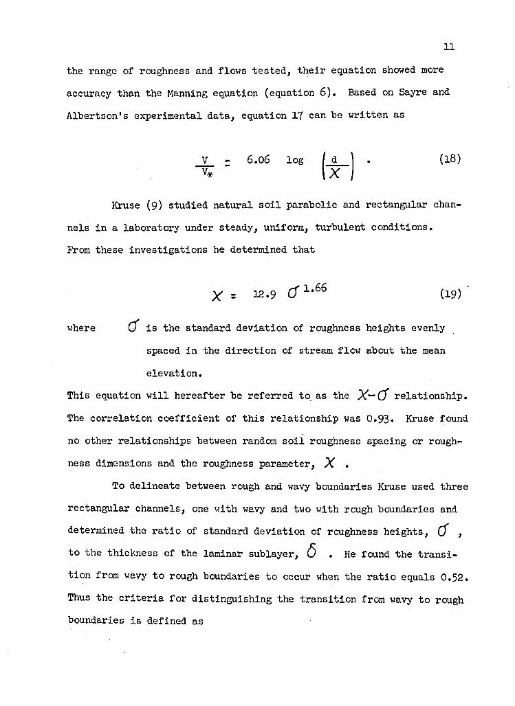
the range of roughness and flows tested, their equation showed more

accuracy than the Manning equation (equation 6 )♦ Based on Sayre and

Albertson’s experimental data, equation 17 can be written as

11

V - 6.06 log / dv* \ X

(18)

Kruse (9) studied natural soil parabolic and rectangular chan­

nels in a laboratory under steady, uniform, turbulent conditions.

From these investigations he determined that

x = 12.9 c f 1 ,66 (19)

where Cf is the standard deviation of roughness heights evenly

spaced in the direction of stream flow about the mean

elevation.

This equation will hereafter be referred to as the X~~(3 relationship.

The correlation coefficient of this relationship was 0.93• Kruse found

no other relationships between random soil roughness spacing or rough­

ness dimensions and the roughness parameter, X .

To delineate between rough and wavy boundaries Kruse used three

rectangular channels, one with wavy and two with rough boundaries and

determined the ratio of standard deviation of roughness heights, Cf ,

to the thickness of the laminar sublayer, (5 * He found the transi­

tion from wavy to rough boundaries to occur when the ratio equals 0 .52.

Thus the criteria for distinguishing the transition from wavy to rough boundaries is defined as

where

^ > 0.52

6 r n .6 V/r*

12

(21)

(20)

Results from his study indicated that the transition from laminar flow

to turbulent flow was at a Reynolds number of 500, where the Reynold's

number is determined by

Re : a v / y . (22)

To determine the constant of integration of Keulcgan's equation

for rough boundary (equation 16), Kruse arbitrarily replaced the term

log (R/k) by log (O' /r ), a measure of relative roughness, and plotted

C / V T versus log ( C T / r ) . He found that for all but one of his chan­

nels the plot would have a slope greater than 5*15* Kruse then chose

the value of 6.06 which agrees with Sayre and Albertson's equation.

Kruse, Huntley, and Robinson (10) showed that the maximum rela­

tive error in predicting flow depth in a rectangular channel was 2%.5

percent, which is equivalent to a 46 percent error when using Manning's

equation. They went on to show that for some rough channels, errors

in Manning's n of 70 percent could result at low flow depths.

Heermann (3) applied the relationship and criteria established

by Kruse to controlled field conditions. He tested the X ~ 0 ’ rela­

tionship for both rectangular and parabolic channels under steady flow

conditions and found that the X — O' relationship was best described

for his conditions when

13

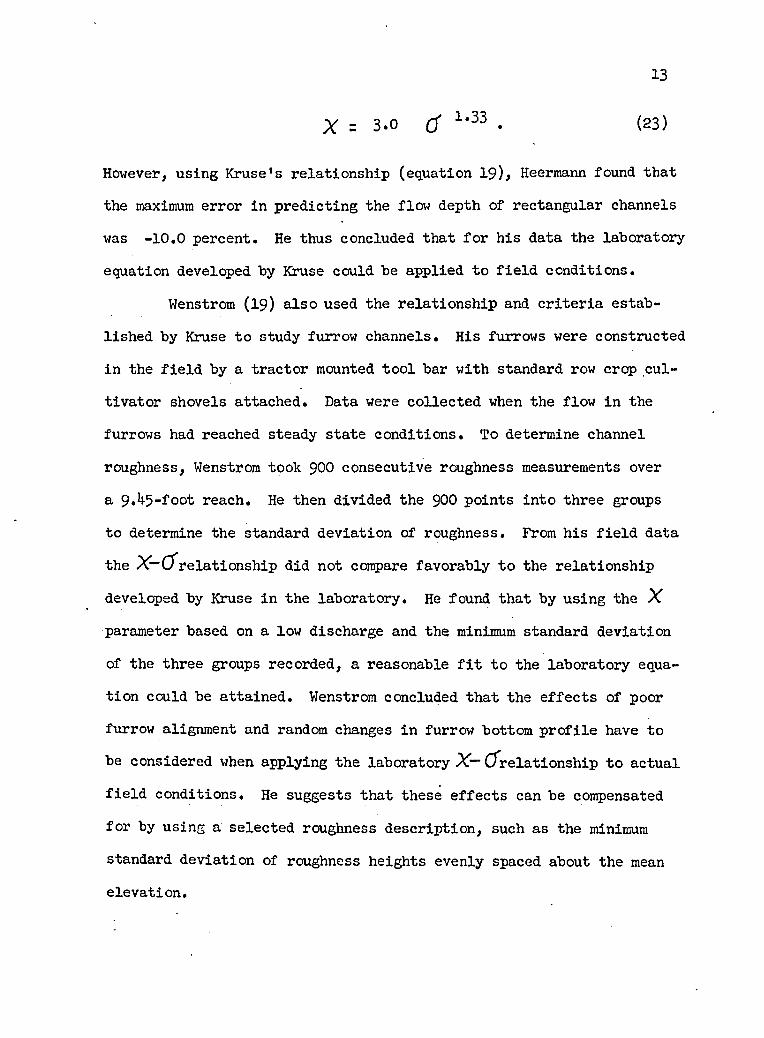
X = 3 .0 Cf 1,33 • (23)

However, using Kruse’s relationship (equation 19), Heermann found that

the maximum error in predicting the flow depth of rectangular channels

was -10.0 percent. He thus concluded that for his data the laboratory

equation developed by Kruse could be applied to field conditions.

Wenstrom (19) also used the relationship and criteria estab­

lished by Kruse to study furrow channels. His furrows were constructed

in the field by a tractor mounted tool bar with standard row crop cul­

tivator shovels attached. Data were collected when the flow in the

furrows had reached steady state conditions. To determine channel

roughness, Wenstrom took 900 consecutive roughness measurements over

a 9•^5-foot reach. He then divided the 900 points into three groups

to determine the standard deviation of roughness. From his field data

the X — O'relationship did not compare favorably to the relationship

developed by Kruse in the laboratory. He found that by using the X parameter based on a low discharge and the minimum standard deviation

of the three groups recorded, a reasonable fit to the laboratory equa­

tion could be attained. Wenstrom concluded that the effects of poor

furrow alignment and random changes in furrow bottom profile have to

be considered when applying the laboratory X— Cfrelationship to actual field conditions. He suggests that these effects can be compensated

for by using a selected roughness description, such as the minimum

standard deviation of roughness heights evenly spaced about the meanelevation.

14

Heermann, Wenstrom, and Evans (6 ) reported that the standard

deviation of 100 roughness height measurements instead of 300 roughness

height measurements used in their studies would give a better comparison

to the empirical X — (5 relationship developed by Kruse. In their work

100 roughness measurements evenly spaced span approximately one foot

which agrees with Kruse’s randomly selected one foot records. Heermann

et al. also sought other statistical methods of improving the X — Cf

relationship but none were found. They also reported that the relation­

ship tended to be independent of the three soil types. Port Collins

loam, Cass fine sandy loam, and Billings silt clay loam, used in their

study.

Heermann (4) felt that the prediction of channel roughness

could be improved if a spacing parameter was included with the height

parameter. He conducted a study using sinusoidal roughnesses of three

amplitudes each with three wave lengths cast inside six-inch steel

pipes. Air was used as the fluid. The conclusion reached from the

experimental data showed that a longitudinal length parameter need

not be included in the characterization of surface roughness. Using

data from other researchers, Heermann showed the same X — Cf rela­

tionship from random soil roughness could be obtained by using spheres

and hemispheres to roughen the boundary. Cube and baffle roughness

required an idealization of an enveloping spherical shape to obtain

the same X — CT relationship as developed by Kruse.

15Infiltration

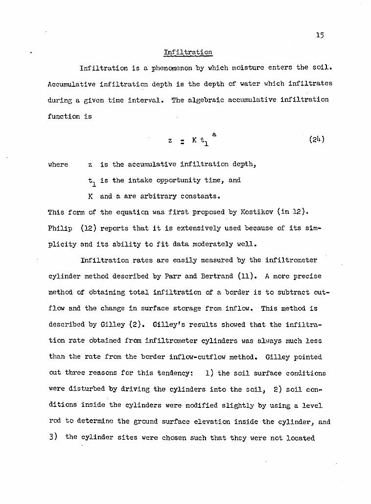
Infiltration is a phenomenon by which moisture enters the soil.

Accumulative infiltration depth is the depth of water which infiltrates

during a given time interval. The algebraic accumulative infiltration

function is

z - K tx a (24)

where z is the accumulative infiltration depth,

t^ is the intake opportunity time, and

K and a are arbitrary constants.

This form of the equation was first proposed by Kostikov (in 12).

Philip (12) reports that it is extensively used because of its sim­

plicity and its ability to fit data moderately well.

Infiltration rates are easily measured by the infiltrometer

cylinder method described by Parr and Bertrand (ll). A more precise

method of obtaining total infiltration of a border is to subtract out­

flow and the change in surface storage from inflow. This method is

described by Gilley (2). Gilley’s results showed that the infiltra­

tion rate obtained from infiltrometer cylinders was always much less

than the rate from the border inflow-outflow method. Gilley pointed

out three reasons for this tendency: l) the soil surface conditions

were disturbed by driving the cylinders into the soil, 2 ) soil con­

ditions inside the cylinders were modified slightly by using a level

rod to determine the ground surface elevation inside the cylinder, and

3) the cylinder sites were chosen such that they were not located

16over a crack in the soil. He felt the third reason could he consid­

ered the most important

CHAPTER 3

EQUIPMENT AND PROCEDURE

All experimental irrigations used in this study were conducted

at the Agricultural Engineering Irrigation Laboratory, University of

Arizona Agricultural Experiment Station, Campbell Avenue Farm, Tucson,

Arizona. A precision field border was used to study roughness during

border irrigation. The border was free of vegetation for several

years prior to the study.

Equipment

Delivery System

Water used for irrigation was obtained from a well and passed

through a large sump. The runoff from the border during irrigations

was pumped back to the sump and recirculated to the border. No mea­

surements were made of sediment concentrations in the runoff water.

A four-inch Sparling meter with both a rate meter and total­

izer was used to measure the water pumped to the border. At the bor­

der head a plastic lined stilling pond was used to receive the water.

A standard 2x4 timber was used for a sill to insure introduction of a

constant depth of water across the entire width of the border.

Runoff System

The tail water was collected in a pond similar to the head

stilling pond. The elevation of this tail sill was adjusted to

17

18compensate for soil subsidence during an irrigation and to maintain

an approximate uniform flow depth near the end of the border.

The border outflow was measured with a fiber glass critical

depth flume of the type developed at the U.S. Water Conservation Lab­

oratory in Phoenix, Arizona (13)# The flume has a sixty-degree

V-shaped critical section and is capable of measuring flow in the range

from 0.001 to 8.0 cubic feet per second. Depth of flow through the

flume was measured in a stilling well equipped with a float and Bel­

fort water stage recorder.

Precision Field Border

The precision field border used is bounded by two concrete

curbs 345 feet long spaced 19.33 feet apart (inside to inside). The

curbing has a nominal 8-inch by 20-inch cross section with approxi­

mately 5 inches extending above ground level. The top of the curbing

is at an approximate 0.07 percent slope. It was feasible to use only

300 feet of the border.

Scissor type automotive jacks mounted on top of the curbing

at 15-foot intervals support steel rails which provide a track for a

20-foot wide rolling carriage or trolley. The rails run the entire

length of the curbing and can be adjusted, using the jacks, to a

variety of slopes. The rails were set at 0.1 percent slope for this

study. Bench marks were established on the curbing at the base of

each jack to facilitate checking the rail slope.

The trolley provides a mounting for a pair of steel blades

used to plane the border to the desired slope and for a small garden

type rotary tiller used between irrigations. It also serves as a

working platform for making measurements before, during, and after

each irrigation.

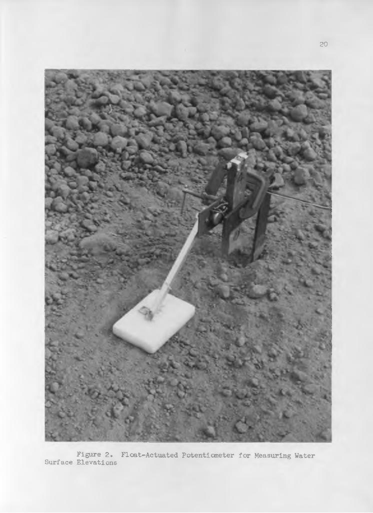
Floats and Recorders

Water surface elevations were measured with float-actuated

potentiometers wired to remote recorders. The potentiometers were

logarithmic taper, Ohmite Type AB, with a 0 to 50,000 ohm range. A

9 l/8-inch lightweight aluminum channel arm was connected rigidly to the potentiometer shaft and pin connected to a 1-inch thick styrofoam

float 6 inches long by 4 inches wide (Figure 2). Spirit levels were

mounted on the float devices so that they could always be installed at

the same orientation. Sun shades were used over the potentiometers to

reduce effects of high temperatures on potentiometer resistance.

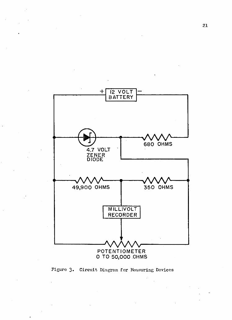
A circuit (Figure 3) was designed with an approximate zero to

0 .350-foot elevation measurement corresponding to a zero to 100 milli­

volt reading on the recorder. The circuit is powered by a 12-volt

automotive battery. A one-watt 4.7 volt zener diode (* 10$ accuracy)

reduced and regulated the voltage at approximately 4 volts.

A total of fourteen measuring devices were built and used in

the study. They were calibrated by curve fitting to the empirical equation.

elevation (ft.) = B^+Bg mv+B^ mv2 + B^ mv3 + B^ e™ + B^ e"mV (2 5)

where mv is the millivolt reading, and

Bl> Bg, Bg, B^, B^, and Bg are constants.

19

20

Figure 2. FIcat-Actuated Potentiometer for Measuring Water Surface Elevations

12 VOLT BATTERY

VW\A6 8 0 OHMS

4.7 VOLTZENERDIODE

VW\A-4 9 , 9 0 0 OHMS

vVXAA-3 5 0 OHMS

MILLIVOLTRECORDER

- ^ W W V -POTENTIOMETER

0 TO 5 0 , 0 0 0 OHMS

Figure 3» Circuit Diagram for Measuring Devices

22Three of the water surface elevation measuring units were

adaped to record changes in the soil surface elevation during irriga­

tion by exchanging their styrofoam floats for sheet metal pads. The

pads were constructed of l8-gauge steel sheets 7 inches long by 2 l/4

inches wide with the ends curved slightly upward. This pad satisfac­

torily followed changes in the border ground surface elevation during

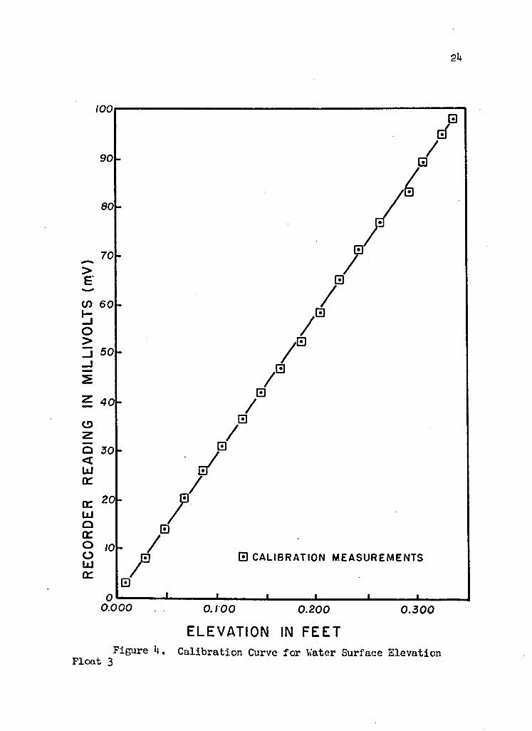
irrigation.Table 1 lists the calibration constants of equation 25 for the

eleven water surface elevation floats and the three soil surface ele­

vation pads. Also listed is the standard error in feet of the cali­

bration equations. The devices have an average maximum standard error

of i 0.003 feet. The calibration curve for water surface elevation

float 3 and the calibration measurements are shown in Figure 4.

Four strip chart recorders, Varian Model G-11A with A-2 input

chassis, were used to record the millivolt readings from the devices.

Four switching boxes permitted manual selection of a recording from

any one of four devices on one instrument at a given time.

Soil Profile Probe

A roughness measuring device (5), soil roughness probe, de­

veloped and built at Colorado State University, Fort Collins, Colo­

rado, was used to measure soil surface roughness heights for this

study. The probe was not used directly on the border, but rather on

castings made of the soil surface before and after each irrigation.

The probe was adapted to read the soil castings as shown in Figure 5.

The probe was fitted to a cart which rolls on a smooth horizontal

Table 1. Values of Device Calibration Constants Used in Equation 25

B-lCxIO"1) B2(xlO'"3 ) B3(xlO"5) Bi^xlO"7 ) B5(xlO”lf5) b6standard

error -(ft.)

Water Surface Elevation Float

1 3.2956 5.2954 -3.2334 1.5463 1.1663 0.00262 2.9065 3.6972 -0.4867 0.2774 - 0.7411 0.00263 2.1113 3.5345 - -0.0893 - «■ 0.0018k 2.1880 4.7959 -0.9333 - 3.7453 1.7368 0.00425 4.0495 5.4020 -2.8929 1.2702 0.0325 . 0.00256 2.6566 4.1130 -0.2641 - - 0.0544 0.00377 2.4822 3.7727 - 0.2504 - 3.4910 0.00268 2.5308 3.6885 - - - 0.0738 0.00369 3.6434 6.4719 -5.5989 3.0622 - 1.4765 0.004110 3.1802 5.7123 -3.5035 1.9347 ~ 2.6258 0.003811 2.0310 4.6154 -2.2022 1.1241 - 0.1144 0.0030

Soil Surface Elevation Pad

1 2.7410 5.1640 -2.4372 1.3253 0.0286 0.00322 2.2825 5.7558 -3.6051 1.8994 -0.2398 0.0561 0.00283 3.5871 6.2278 -3.9504 1.8535 0.1611 0.0033

REC

OR

DER

R

EA

DIN

G

IN

MIL

LIV

OLT

S (

mV

)

2k

0 CALIBRATION MEASUREMENTS

0.000 O.IOO 0.200 0.300

ELEVATION IN FEETFigure 1». Calibration Curve for Water Surface Elevation

Float 3

25

Figure 5* Soil Roughness Probe Ready to Read a Soil Cast

26surface. The soil casting was placed with the rough side up and 100

probe readings taken in this position. Six readings, three at each

end of the soil casting, were also taken to the horizontal surface to , determine average thickness of the casting, a dimension used in later

analysis.

Procedure

A rather long process is involved in making an irrigation test.

A minimum span of three days is required, and depending upon the amount

of soil preparation needed, much more time might be used. Additional

time is required to determine soil roughness and prepare data for

analysis.

Border Preparation

All irrigations were made on soil tilled with a garden type

rotary tiller mounted to the trolley. Trolley handbrakes to control

forward motion at a constant rate assured uniform tillage throughout

the border.

With tilling completed, horizontal blades were mounted on the

trolley to plane the surface by repeated passes over the border. Each

pass with the leveling blades reduced the roughness, so the number of

passes made was used as a control of initial surface roughness for a

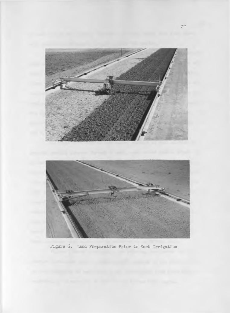
particular irrigation. Figure 6 shows the land preparation sequence use in this study.

The border head and tail sills were then installed 308 feet

apart. This allowed 4 feet at each end of the border to minimize

effect of flow over the head and tail sills on the measuring devices

2?

Figure 6. Land Preparation Prior to Each Irrigation

28at each end of the border. The head and tail ponds were then lined

with plastic to eliminate losses oitside the border.The water surface elevation floats and soil surface elevation

pads were set at selected stations along the center of the border and

wired into the recording circuit. The first water surface elevation

float was placed 4 feet from the head sill where bench marks were es­

tablished and the border begins. The remaining ten water surface ele­

vation floats were placed 30 feet apart, each at a bench mark location.

The stations were numbered 1 through 11 in a downstream direction. The

three soil surface elevation pads were set midway between stations 1

and 2, 5 and 6, and 9 and 10.

Castings were made of the border surface at each station by

pouring casting plaster through a small mesh screen into a 3-inch by

15-inch mold made of 1-inch angle iron. The small mesh screen satis­

factorily reduced soil disturbance when pouring. The mold was leveled

with a carpenter’s level prior to pouring. After pouring, the upper

side of the casting was planed smooth. All castings were made with the

longer dimension of the mold in the direction of stream flow. The lo­

cation of the casting was at a point that best described the immediate

area near the center of the border, and in line with the float and

bench marks. Photographs were taken of each casting in the border.

These castings will hereafter be referred to as BEFORE casts.

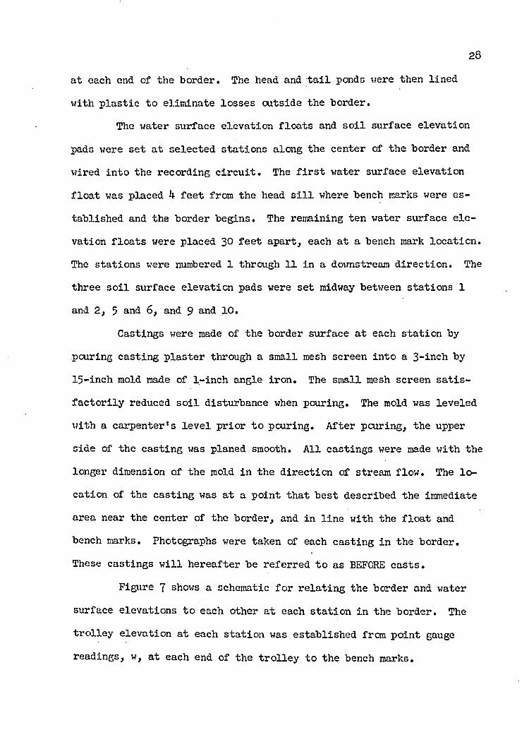
Figure 7 shows a schematic for relating the border and water

surface elevations to each other at each station in the border. The

trolley elevation at each station was established from point gauge

readings, w, at each end of the trolley to the bench marks.

TROLLEY

BENCHMARK

NOT TO SCALE

Figure 7. Schematic for Determining Border Elevation Control

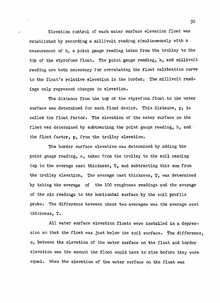
30Elevation control of each water surface elevation float was

established by recording a millivolt reading simultaneously with a

measurement of h, a point gauge reading taken from the trolley to the

top of the styrofoam float. The point gauge reading, h, and millivolt

reading are both necessary for correlating the float calibration curve

to the float’s relative elevation in the border. The millivolt read­

ings only represent changes in elevation.

The distance from the top of the styrofoam float to the water

surface was determined for each float device. This distance, p, is

called the float factor. The elevation of the water surface on the

float was determined by subtracting the point gauge reading, h, and •

the float factor, p, from the trolley elevation.

The border surface elevation was determined by adding the

point gauge reading, c, taken from the trolley to the soil casting

top to the average cast thickness, T, and subtracting this sum from

the trolley elevation. The average cast thickness, T, was determined

by taking the average of the 100 roughness readings and the average

of the six readings to the horizontal surface by the soil profile

probe. The difference between these two averages was the average cast thickness, T.

All water surface elevation floats were installed in a depres­

sion so that the float was just below the soil surface. The difference,

u, between the elevation of the water surface on the float and border

elevation was the amount the float would have to rise before they were

equal. When the elevation of the water surface on the float was

greater than the border elevation a flow depth existed. Permitting

the floats to pass below the soil surface facilitated measurement of

advance and recession times.The soil surface elevation pads rested on the undisturbed soil

surface. Differences in millivolt readings represented changes in the

border elevation at each station.Three infiltrometer cylinders were installed at equal inter­

vals along the border in preparation for ponded infiltration tests during the irrigation. Soil samples at three equal intervals along

the border were taken at six-inch depth intervals for two feet for

gravimeteric soil moisture measurements prior to the irrigations.

Irrigation Procedure

Water was introduced into the border head pond and all re­

corders were started at the moment water reached station 1. This

point in time was noted as zero for the irrigation.

The inflow Sparling meter readings were recorded at time zero

and every five minutes thereafter. The flow rate was kept constant by a valve.

Since three to four floats were measured by one recorder, only

the rising portion of the hydrograph was continuously recorded. The

remaining portions of the hydrograph were recorded intermittently,

usually once every minute. Occasional point gauge measurements from

the trolley to the water surface were made beside al1 water surface

elevation floats during the irrigation to verify the float readings.

31

32As the water reached each infiltroraeter cylinder, ponded in­

filtration measurements were made using a hook gauge. A field observ­

er also noted the time water reached each station (advance), water

temperature at both the border head and tail ponds several times during

the run, and the time water receded from each station (recession).

The observer considered recession to occur when approximately one-half

the surface surrounding the station was covered with water and the

remaining half was free of surface water.

Border inflow ended when water stopped flowing over the head

sill. Measurements were continued until border outflow approached

0.001 cubic feet per second and the flow had recessed from all

stations.

Post-Irrigation Procedure

Several hours after the irrigation was complete, plaster casts

of the soil surface at all stations were again made as described pre­

viously. This delay was required to allow the soil surface to solidify

so it could support the cast molding and plaster. Photographs were

again taken of all soil castings in the border. These castings will

hereafter be referred to as the AFTER casts.

Elevation control of the water surface elevation floats was

again established by the procedure outlined previously. These mea­

surements both before and after the irrigation enhanced evaluation of

measurement errors.

Soil samples were again taken at three locations along the

border at six-inch intervals for two feet to make gravimeteric soil

33moisture measurements after the irrigation. All soil surface castings

(eleven BEFORE and eleven AFTER castings) were washed and roughness

measurements were made on each by using the soil profile probe.

CHAPTER 4

BORDER FLOW ANALYSIS

To analyze and compute the roughness coefficients which exist

during border irrigation it was necessary to determine the following

parameters: l) slope, 2) flow depth, 3) hydraulic radius, and 4)

average velocity. To expedite the determination of these parameters

a FORTRAN IV program was written which converts basic field data into

consistent units and performs most of the calculations.

For analysis the border was divided into ten equal 30-foot

reaches demarcated by the eleven surface elevation measuring stations.

The irrigation was divided into time periods. The first ten periods,

usually less than 6 minutes each, were defined by the time required

for the water front to advance across each of the ten reaches plus 0.1

minute and the remaining periods were established at 1, 2, 4, or 10

minutes depending on the rate of change of the border outflow. The

shorter periods were used when the border outflow was changing rapidly.

The addition of 0.1 minute to each of the first ten periods will be ex­

plained later.

Slope

Three slopes: channel bed, water surface, and total energy line

are referred to when discussing open channel flow. Chow (l) states

that when the bed slope is less than 5 degrees and the flow is steady

34

35and uniform, all three slopes are approximately equal. The bed slope

used in this study was approximately 0.1 percent (less than 1 degree)

and the flow was unsteady and ncnuniform. It will be shown in the fol­

lowing chapter that after the water had advanced the length of the bor­

der the three slopes are approximately equal. Thus uniform flow

equations were used to determine roughness during border irrigation.

As discussed previously, the border elevation at each station

was determined from a point gauge reading to the soil casting top and

the average cast thickness (Figure 7)• Slope, S^, was computed from

a least squares regression line through the eleven border elevations

determined from the soil castings prior to the irrigation. The border

elevatioi) values were then corrected to fit the least squares regres­

sion line. The border elevations after the irrigation were also cor­

rected to a least squares regression line through the border elevations

determined from the AFTER castings.

The average difference between the border elevations at the

beginning and end of the irrigation was the total change in the bor­

der surface or subsidence. This subsidence was divided into two parts;

that which occurred during the irrigation and that occurring after the

irrigation between the time when all stations recessed and the soil

castings were poured. The division of these two values of subsidence

was computed by the average change as measured by the three pads for measuring soil surface elevations.

The three subsidence measurements from the soil surface eleva­

tion pads during the irrigation were then averaged and plotted on a

single graph. The magnitude of total subsidence from the graph was

corrected to equal the border subsidence during the irrigation as de­

termined from the soil castings. Only the average of these three sub­

sidence measurements was used to give the timewise distribution of

subsidence during the irrigation and to determine the amount of subsi­

dence that occurred during the irrigation and the amount that occurred

after the irrigation.The border elevations for each period at each station during

the irrigation were then computed by using the average adjusted sub­

sidence graph. Although the border elevations during the irrigation

were changing due to subsidence, the slope, S^, for computing rough­

ness coefficients was kept at the constant value as determined from

the least squares regression line through the initial border eleva­

tions. This assumption will be discussed in more detail in the fol­

lowing chapter.

Flow Depth

The flow depth, d, in the border is the normal distance be­

tween the channel bed and the water surface. For small slopes and

flow depths the normal and vertical depths are approximately equal.

Flow depth hydrographs at each station were determined by

subtracting the border elevations from the water surface elevations.

Water surface elevations were computed from the recorded float data

and then corrected by a constant amount. The correction for each

float was the average difference between the water surface elevations

as measured by the floats and the point gauge readings as measured

from the trolley to the water surface during the irrigation. The water

37surface elevations measured by the point gauge readings from the

trolley were assumed to be correct, because point gauge measurements

were the standard for calibrating the water surface elevation floats.

The flow depth during any period was assumed to be the average of flow

depths at the beginning and end of that period.

Hydraulic Radius

Hydraulic radius, R, was determined for each station and period

by dividing the flow area by the wetted perimeter. Wetted perimeter

was found by adding the border width and twice the flow depth. The

flow area was the average of the flow areas at the beginning and end

of each period.

Average Velocity

The average velocity, V, past each station during each period

was determined from the continuity equation,

AVERAGE VELOCITY = FLOW RATE / FLOW AREA. (26)

The flow rate past each station was determined for each period by using

the equation,

OUTFLOW z INFLOW - CHANGE IN CHANNEL STORAGE - INFILTRATION, (27)

and dividing the outflow by the duration of the period.

Equation 27 was solved for the outflows from all reaches and

periods by using measured or computed inflow, measured change in sur­

face storage, and an infiltration function. Inflow past the first

station and into the first reach was the measured border inflow, but

inflow into the remaining reaches was the computed outflow from the

upstream reach. Changes in surface storage in a reach were computed

38from the changes in flow depths as indicated "by the upstream and

downstream flow depth hydrographs. Infiltration into each reach dur­

ing each period was determined by the infiltration function, equation

2k, where the constants, K and a, were initially determined from the

analysis of the infiltrometer data and later revised by using a vol­

ume balance analysis of the flow of water along the border. The

analysis required two assumptions during the advancing phase that

applied only to the reach over which the water had just advanced.

The assumptions are:1. The leading edge of water was a vertical wall of water. The

height of the vertical wall of water was assumed to be the

depth of water at 0.1 minute after the water had been at the

station. This was the reason for adding 0.1 minute to each

of the first ten periods. During this time the water had ad­

vanced a small distance, about one foot, past the station.

In the volume balance, this volume of water was neglected

because it was estimated at approximately 3 percent of the

total volume over the entire reach.

2. The infiltration volume as computed by equation 2k was as­

sumed to occur over the entire reach for the total period.

Results from irrigations analyzed showed that 20 to 60 per­

cent of the total infiltration into a reach occurred during

the period a reach was first wetted. It was felt that most

of this initial infiltration occurred when the water first

covered the surface and filled the surface voids.

39Basically the volume balance approach was accomplished by de­

termining for a period the outflows for each reach starting with reach

1 and continuing until outflows for all the reaches had been computed.

At the end of each period, another volume balance was made of the en­

tire border using measured inflow, measured outflow, and measured

change in surface storage. Thus two values of border infiltration

were computed for each period; one value was the summation of infil­

tration for each reach as estimated from the infiltration function,

and the other value was the infiltration as computed by the volume

balance of the entire border.

The following example will illustrate how the volume balance

analysis was made. During the first period the water had advanced to

station 2. Referring to Figure 8, the inflow into reach 1 during

period 1, dQ^ is the measured border inflow. The change in sur­

face storage, dS , was computed from the flow depths at stations 1 1>1and 2 at the end of the period. The infiltration, dl , was esti-1,1mated by solving for the infiltration depth from equation 24. Since

there are no other reaches with flow, total infiltration into the bor­

der was found by subtracting the measured change in surface storage,

dS , from the measured inflow, dQ . Thus two values of infiltra-1,1tion were determined; one estimated by the infiltration function and

the second computed by the measured inflow minus measured change in surface storage.

The inflow into reach 1, dQ^ was the measured border in­

flow during the second period only. The computed outflow from reach 1,

was computed by subtracting the change in surface storage. dS1,2

n o t to s c a l e

I I I

REACH 2REACH l STATION 4

STATION 3STATION 2

STATION 1during Advanceof Border IrrigationCross Section

and infiltration, dl , from the measured inflow, dQ . The change1,2

in surface storage, dS , was computed by finding the change in1,2depths between the end of periods 1 and 2 at stations 1 and 2. The

infiltration, dl , was estimated by applying the infiltration func-1,2tion during the second period. The change in surface storage, dS

and infiltration, dl in reach 2 were also determined. An estimate2,2of total infiltration into the border during the second period was the

summation of dl, _ and dl . The value of total infiltration into1,2 2,2the border by volume balance was determined by subtracting the total

measured change in surface storage, dS plus dS , from the mea-1,2 2,2sured border inflow dQ

During the third period the outflow from reach 1, dQ , was2,3

equal to the measured inflow, dQ , minus the measured change in

surface storage, dS , and infiltration, dl . The outflow from1,3 1,3

reach 2, dQ , was equal to the computed inflow, dQ , minus the3,3 2,3'measured change in surface storage, dS , and infiltration, dl .2,3 2,3The values of dS and dl_ , are similarly determined. An estimate3,3 3,3of total infiltration into the border by the infiltration function

during the third period was the summation of dl . dl „, and dl .1,3 2,3 3,3The value of infiltration by volume balance was determined by sub­

tracting the total measured change in surface storage, dS plus1,3

dS plus dS , from the measured border inflow, dQ. .2,3 3,3 x,3

The volume balance was continued in this manner until the

eleventh period. At the beginning of the eleventh period border out­

flow started. To determine infiltration into the entire border, both

the measured change in surface storage for all ten reaches and the

42

“border outflow were subtracted from the measured border inflow. The

computations continued until flow had recessed from all stations and

border outflow stopped.After all periods were analyzed in this manner, an evaluation

of the infiltration function was made. The infiltration function con­

stants, K and a, were revised and the computations recycled. The pro­

cess was continued until an infiltration function was obtained which

agreed most closely with the volume balance for each period, and also

closely satisfied the total volume balance for all periods.

At this point the total border infiltration as determined by

the equation was compared to the total border infiltration as deter­

mined by volume balance. If the two values differed by more than two

cubic feet, an adjustment factor was determined from the ratio of these

two total border infiltrations. This adjustment factor was multiplied

times the constant K and the computations were again made. The total

border infiltration by equation and volume balance were then exactly

the same.

The flow rate past each station for each period was determined

by dividing the outflow from the upstream reach by the duration of the

period. Average velocity was then computed by employing equation 26.

Roughness Coefficients

Roughness coefficients were determined from uniform flow

equations for each period and station if the flow conditions met Kruse’s

criteria. His criteria require turbulent flow, the Reynolds number

greater than 500 (equation 22), and a rough boundary determined by the following equations

4:

9^5 ^ 0.52 (20)

where (5 — 11.6 2V/V* • (21)

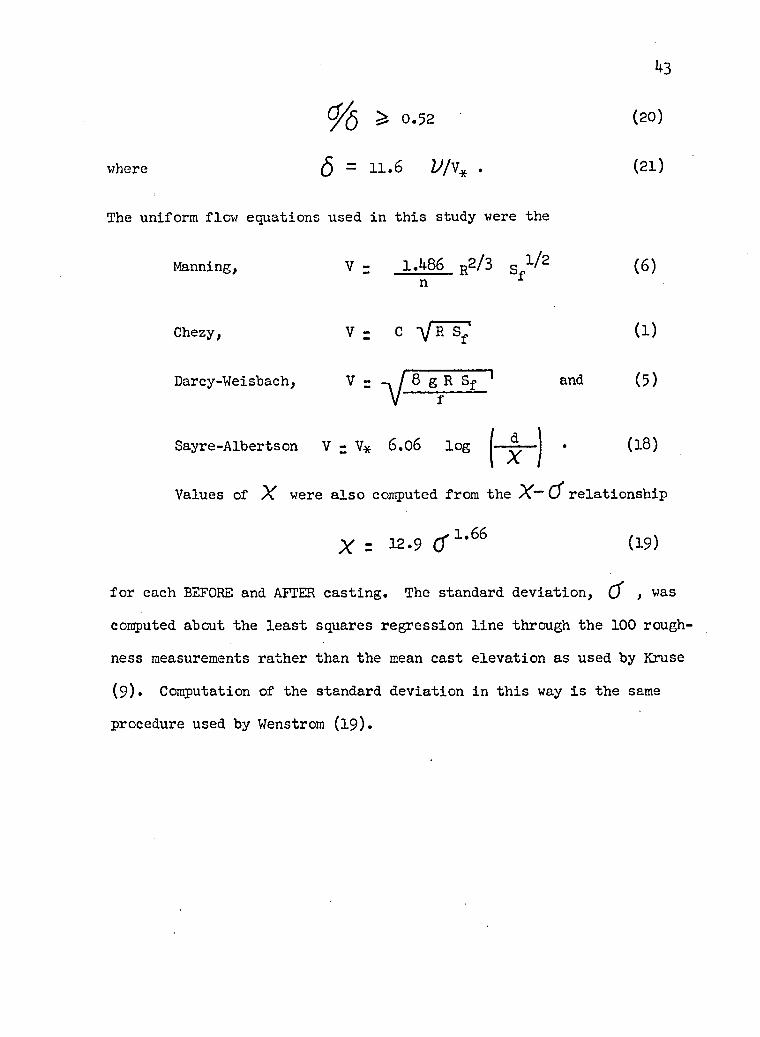
The uniform flow equations used in this study were the

Manning, V - 1.486 p2/31 Sf1/2 (6)n

Chezy, V = C V R Sf' (1)

Darcy-Weisbach, V 2 -yj 8 g R Sf 11 and (5)

Sayre-Albertson V 2 V* 6.06 log( x ) • (18)

Values of % were also computed from the (f relationship

x = 12.9 O'1,66 (19)

for each BEFORE and AFTER casting. The standard deviation, Cf , was

computed about the least squares regression line through the 100 rough­

ness measurements rather than the mean cast elevation as used by Kruse

(9). Computation of the standard deviation in this way is the same

procedure used by Wenstrom (19).

CHAPTER 5

PRESENTATION OF DATA

Eleven irrigations were conducted for this study, but the hy­

draulic data from only Irrigations 8, 9j 10, and 11, will be presented.

The water surface elevation hydrographs determined from the first seven

irrigations were inaccurate and thus cannot be analyzed by the volume

balance procedure described in the previous chapter. However, data

from the BEFORE and AFTER casts from all eleven irrigations will be

presented and analyzed.The results of Irrigations 8, 9> 10, and 11 are summarized in

Table 2. The border slope, Sf, is that which was determined from the

least squares regression line through the border elevations computed

from the BEFORE casts. The infiltration functions given are those

which agreed exactly with the volume balance analysis.

The presentation of data that were measured or computed for

each station and period will be in the following form: l) one or

more periods were averaged to give uniform time intervals of ten

minutes, and 2) stations 2, 3, and 4, stations 9, 6, and 7, and sta­

tions 8, 9, and 10, were averaged during these time intervals to give

three new stations at 60 feet, 150 feet, and 240 feet respectively.

Data will be shown for the border inflow interval only because once

inflow stops, the flow becomes very unsteady and nonuniform, and ac­

curate measurements become very difficult.

44

Table 2. Summary of Data for Irrigations 8, 9, 10, and 11

Irrigation Number

8 9 10 11

Date 13 July 70 10 Aug. 70 21 Aug. 70 31 Aug. 70Number of reaches 10 10 10 10Length of reach (ft.) 30 30 30 30Border slope, S^, (ft./ft.) 0.0010 0.0010 0.0011 0.0010Inflow rate (c.f.s.) 0.365 0.502 0.697 0.505Total inflow (c.f.) 3975 5409 7483 5428Total outflow (c.f.) 2231 3632 6654 4158Total infiltration (c.f.) 17W 1777 829 1270Average infiltration (in.) 3-6 3 .7 1.7 2.6Duration of inflow (min.) 181.4 179.7 179.0 179.3Total advance time (min.) 44.7 41.2 28 .7 39-5Average water temperature (°F) 75.8 78.9 81.3 82.3Total border subsidence (ft.) 0.015 0.036 0.024 0.073Infiltration Equation z - K t^a z is in feet and t^ is in minutes

K 0.0378 0.0468 0.0799 0.0539a 0.394 0.358 0.110 0.244

•F*vn

46

Measured Flow Depths

Tables 3* 4, 5; and 6 list the measured flow depths in feet for

Irrigations 8, 9, 10, and 11 respectively. The flow depths are given

at stations 60, 150, and 240 feet for 17 ten-minute time intervals,

starting ten minutes after introduction of inflow. Flow depths are

shown when both reaches in the section of the border defined by the

station are wetted.Measured flow depths for Irrigation 8, Table 3, show that once

the flow had been at any station for about 40 minutes the flow depth was constant, about 0.048 feet. Flow depths did not increase signifi­

cantly with time after the station was first wetted. For Irrigation 9;

Table 4, the depths show a slight increase in depth with increasing

time. There is also a definite trend of increasing depth with distance

down the border. Depth increases about 0.014 feet from station 60 feet

to station 240 feet. In Irrigation 10, Table 5; the depths remain

fairly constant with time but depth increased from station 60 feet to

station 150 feet. The depths at station 240 feet was consistently,

but only slightly greater than at station 150 feet. Irrigation 11,

Table 6, resembles Irrigation 8, in that the depths do not change

significantly with space. The depths at stations 60 feet and 150 feet

indicate some decrease with time while station 240 feet indicates an increase.

The flow depths for Irrigations 8, 9, 10, and 11 indicate many

possibilities of flow depth combinations with time and space. The

flow depth measurements listed are estimated to be accurate to - 0.005feet.

4?Table 3* Measured Flow Depths for Irrigation 8

Time (min.)Flow Depth in feet

Station 60 ft. Station 150 ft. Station 24o ft.

10 0.03520 0.038 - -30 0.040 0.033 -4o 0.043 0.037 0.02750 0.046 o.o4o 0.0306o 0.048 o.o44 0.03670 0.048 o.o46 0.04180 0.048 o.o46 0.04490 0.049 0.047 0.045

100 0.049 0.047 0.046110 0.049 0.047 o.o46120 0.049 0.047 0.047130 0.049 0.047 0.047140 0.049 0.047 o.o48150 0.049 0.047 0.048160 0.049 0.047 0.048170 0.050 0.047 0.048

Table 4. Measured Flow Depths for Irrigation 9

Time (min.)Flow Depth in feet

Station 60 ft. Station 150 ft. Station 240 ft.

10 0.059 - -20 0.076 - -30 0.077 0.080 -40 0.078 0.082 0.07250 0.078 0.083 0.08260 0.079 0.084 0.08770 0.079 0.084 0.09080 0.079 0.085 0.09190 O.079 0.085 0.092100 0.079 0.083 0.093no 0.080 0.087 0.093120 0.080 0.087 0.094130 0.080 0.088 0.094

l4o 0.079 0.087 0.094150 0.081 0.087 0.094160 0.082 0.090 0.093170 0.082 0.090 0.096

1+8

Table 5* Measured Flow Depths for Irrigation 10

Time (min.)Flow Depth in feet

Station 60 ft. Station 150 ft. Station 240 ft.

10 0.08020 0.095 0.099 -30 0.093 0.108 —40 0.092 0.107 0.10850 0.092 0.106 0.1086o 0.090 0.102 0.106to O.O89 0.099 0.10180 0.090 0.099 0.10390 0.089 0.099 0.103

100 0.088 0.100 0.103110 0.088 0.100 0.102120 0.086 0.098 0.101130 0.086 0.099 0.099140 O.O87 0.099 0.101150 0.087 0.100 0.102160 0.088 0.100 0.102170 O.O87 0.099 0.102

Table 6. Measured Flow Depths for Irrigation 11

Time (min.)Flow Depth in feet

Station 60 ft. Station 150 ft. Station 240 ft.10 - - -20 0.089 - -30 0.086 0.085 -40 0.081 0.084 0.06750 0.080 0.083 0.07460 0.080 0.083 0.07770 0.080 0.081 0.07880 0.080 0.082 0.07890 0.078 0.082 0.078

100 0.076 0.080 0.077110 0.079 0.082 0.075120 0.079 0.082 0.079130 0.079 0.083 0.079l 4o 0.079 0.082 0.079150 0.080 0.084 0.081160 0.078 0.081 0.081170 0.078 0.081 0.080

49

Computed Velocities

The computed velocities in feet per second for Irrigations 8,

9, 10, and 11 are shown in Tables 7, 8, 9, and 10 respectively. The

computed velocities were determined from the volume balance analysis

used in this study. The velocities given are for the same stations

and times as the flow depths.The velocities for Irrigation 8, Table 7 1 indicate a constant

value with time but a decreasing trend with space. Irrigation 9,

Table 8, shows the same trend as Irrigation 8 but the velocity decrease

with space is larger. Irrigation 10, Table 9, also shows similar

trends as Irrigation 8. However, Irrigation 11, Table 10, indicates

that velocities remain relatively constant with time and space.

Water Surface Slopes

Water surface slopes were determined by a least squares re­

gression line through the water surface elevations at each 30-foot

measuring station. Table 11 lists the water surface slopes in feet

per foot for 10 minute time intervals for Irrigations 8, 9) 10 and 11.

Also listed is the slope, S^, that was used in the roughness calcula­

tions. Only those stations which were wetted were used to determine

the water surface slope during the advance phase.

Once the water had advanced the entire length of the border,

the slopes were a constant value of 0.0010 ft./ft. The total advance

time for all irrigations is listed in Table 2. The slope value of

0.0010 ft./ft. agrees with the slope, S^, used in all irrigations, ex­

cept for Irrigation 10. The slope, S^, used in Irrigation 10 was

50

Table 7* Computed Velocities for Irrigation 8

________ Velocity in feet per s e c o n d ________Time (min.) Station 60 ft. Station 150 ft. Station 240 ft.

10 - - -20 0.43 - -30 0.42 0.38 -4o o.4o 0.38 0.3750 0.38 0.36 0.376o 0.38 0.36 0.3670 0.38 0.35 0.3480 0.38 0.35 0.3390 0.38 0.35 0.33

100 0.37 0.36 0.33110 0.37 0.36 0.33120 0.37 0.36 0.33130 0.38 0.37 0.34i4o 0.38 0.37 0.34150 0.36 0.35 0.32l6o 0.36 0.35 0.32170 0.39 0.39 0.36

Table 8. Computed Velocities for Irrigation 9

- Velocity in feet per secondTime (min.) Station 60 ft. Station 150 ft. Station 240 ft.

10 _

20 0.31 - -

30 0.31 0.26 -40 0.31 0.27 -

50 0.32 0.27 0.2360 0.32 0.27 0.2370 0.31 0.27 0.2380 0.31 0.27 0.2390 0.31 0.27 0.23100 0.31 0.28 0.24

110 0.31 0.28 0.24120 0.31 0.28 0.24130 0.32 0.28 0.24140 0.31 0.27 0.24150 0.31 0.27 0.24160 0.32 0.28 0.24170 0.31 0.27 0.25

51Table 9* Computed Velocities for Irrigation 10

Velocity in feet per secondTime (min.) Station oO ft. Station 150 ft. Station 240 ft.

1020 0 .36 - -30 0.37 0.32 -

40 0 .38 0.33 0.3250 0.38 0.34 0.336o 0.39 0.35 0.3470 0.40 0.35 0.358o o.4o O .36 0.3490 o.4i O .36 0.35

100 o.4i O .36 0.35110 0.4l 0.37 0.35120 0.41 0.36 0.35130 0.4l O .36 0.35lUo 0.42 0.36 0.35150 0.4l O .36 0.35160 0.42 O .36 0.35170 0.4l O .36 0.35

Table 10. Computed Velocities for Irrigation 11

Velocity in feet per secondTime (min.) Station 60 ft. Station 150 ft. Station 240 ft.

10 _

20 0 .28 - -30 0.30 0 .28 -40 0.30 0 .28 0.3250 0.32 0.29 0.3160 0.32 0.29 0.2970 0.32 0 .30 0.3080 0.32 0 .30 0.3090 0.33 0 .30 0.31

100 0.33 0 .30 0.31110 0.32 0 .30 0.30120 0.33 0.31 0.32130 0.32 0.31 0.31l4o 0.33 0.31 0.32150 0.33 0.31 0.31160 0.32 0.31 0.31170 0.32 0.31 0.31

52

Table 11. Water Surface Slopes for Irrigations 8, 9, 10, and 11

Time (min.)Irrigation number

8 9 10 11

10 0.0012 0.0012 0.0011 0.0009

20 0.0011 0.0010 0.0010 0.0008

30 0.0011 0.0010 0 .0010* 0.0009

40 0.0010 0.0010 0.0010 0 .0010*

50 0 .0010* 0 .0010* 0.0010 0.0010

6o 0.0010 0.0010 0.0010 0.0010

70 0.0010 0.0010 0.0010 0.0010

8o 0.0010 0.0010 0.0010 0.0011

90 0.0010 0.0010 0.0010 0.0010

100 0.0010 0.0010 0.0010 0.0010

110 0.0010 0.0010 0.0010 0.0011

120 0.0010 0.0010 0.0010 0.0010

130 0.0010 0.0010 0.0010 0.0010

i 4o 0.0010 0.0010 0.0010 0.0010

150 0.0010 0.0010 0.0010 0.0010

160 0.0010 0.0010 0.0010 0.0010

170 0.0010 0.0010 0.0010 0.0010Slope, Sj, used in roughness calculations

0.0010 0.0010 0.0011 0.0010

*The first time all eleven measuring stations are used to com­pute the water surface slope

530.0011 ft./ft. Thus the water surface slopes did equal the border

surface slope after the water had advanced the length of the border.

The range of velocities for Irrigations 8, 9> 10, and 11 from

Tables 7, 8, 9, and 10 is from 0.23 to 0.43 feet per second. The

energy in feet of water for this range of velocity is from 0.0008 to

0.0028. The elevation of the total energy line at any point can be

determined by adding the energy due to the velocity to water surface

elevation. Since the energy due to the velocity would change very

little from station to station the slope of the total energy line was

assumed equal to the water surface slope. For this study the slopes

of channel bed, water surface, and total energy line were assumed

identical.

Determination of Flow Regime

Prior to computing roughness coefficients from uniform flow

equations, the flow conditions were checked to verify that they were

turbulent and the channel boundary was rough. Tables 20, 21, 22, and

23 in Appendix A show the average Reynolds numbers for Irrigations 8,

9, 10, and 11. These values were computed by using equation 22. The

minimum value calculated for these irrigations was 1100 while the max­

imum value was 4100. These values exceed the minimum value of 500

recommended by Kruse for turbulent flow.. Thus, flow in all irrigations

presented in this study was turbulent.

Tables 24, 25, 26, and 27 in Appendix A show the &/$ values

for determining if the boundary is rough. These values were calcu­

lated by using equations 20 and 21. For values greater than 0.52 the

boundary is rough. For Irrigations 9* 10, and 11 the values for de­

termining the boundary condition ranged from 1.43 to 3«59» Thus the

boundaries were considered rough. However, the values for Irrigation

8 were less than or only slightly greater than the value of 0.52. Al­

though it is questionable whether the boundary condition for Irriga­

tion 8 is rough, roughness coefficients were computed as if the boundary

was rough.

54

Roughness Coefficients and Parameters

Computed values of Manning’s roughness coefficient, n, are

shown for Irrigations 8, 9, 10, and 11 in Tables 28, 29, 30, and 31 respectively in Appendix B. These values were calculated by using

equation 6. The values of Manning's n ranged from 0.012 to 0.04l.

Tables 32, 33, 34, and 35 in Appendix B list the values of

Sayre-Albertson's roughness parameter, X , which were computed by

using equation 18. The minimum computed value of X } 0.0004, was

for Irrigation 8 and the maximum value was 0.018? for Irrigation 9»

Values for X were also computed from measurements on the BEFORE and

AFTER casts using equation 19. These values are shown in Table 44 of

Appendix B for Irrigations 8, 9, 10, and 11.

Chezy and Darcy-Weisbach roughness coefficients were calculated

by using equations 1 and 5 respectively and are shown in Tables 36 to

43 in Appendix B. Variation in roughness with space and time will be

discussed in more detail in the next chapter.

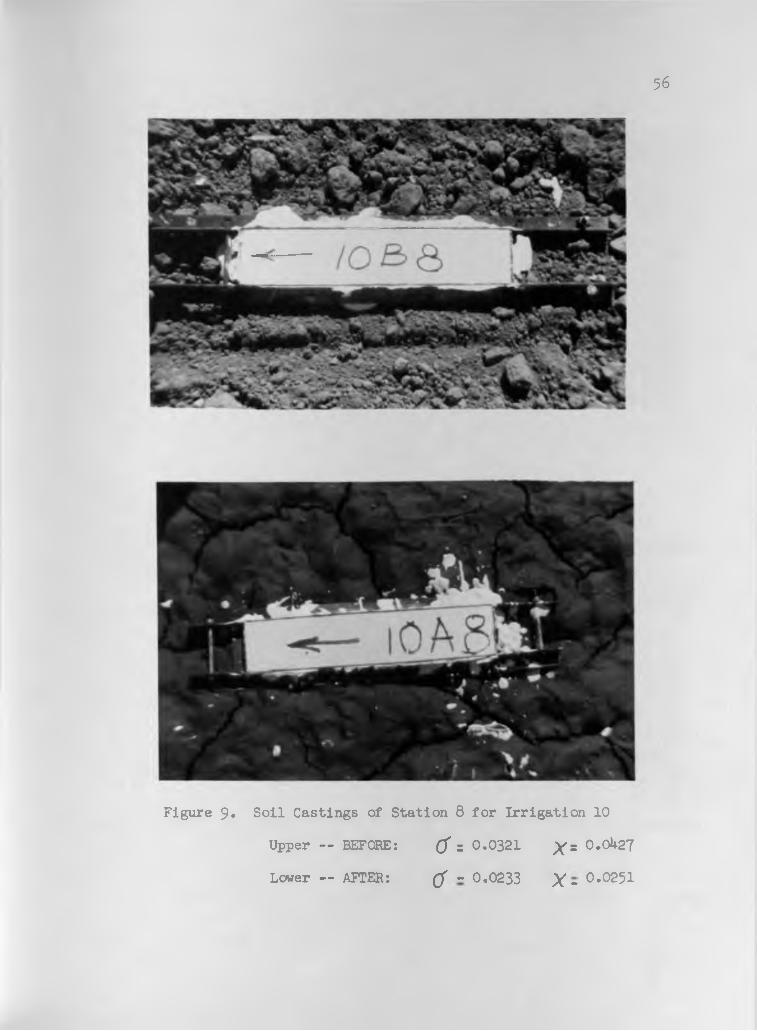
To familiarize the readers with Sayre-Albertson's X values and how these values appear in field conditions, photographs of the

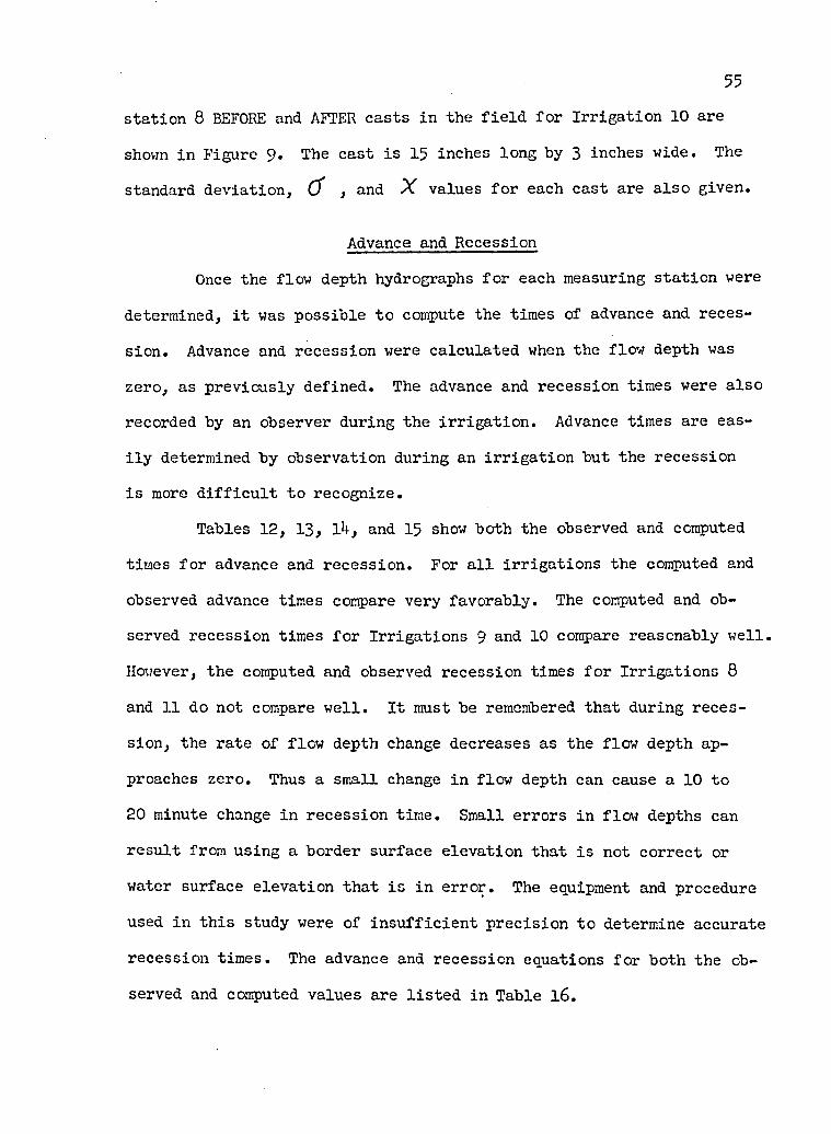
55station 8 BEFORE and AFTER casts in the field for Irrigation 10 are

shown in Figure 9 . The cast is 15 inches long by 3 inches wide. The

standard deviation. O' , and X values for each cast are also given.

Advance and Recession

Once the flow depth hydrographs for each measuring station were

determined, it was possible to compute the times of advance and reces­

sion. Advance and recession were calculated when the flow depth was

zero, as previously defined. The advance and recession times were also

recorded by an observer during the irrigation. Advance times are eas­

ily determined by observation during an irrigation but the recession

is more difficult to recognize.

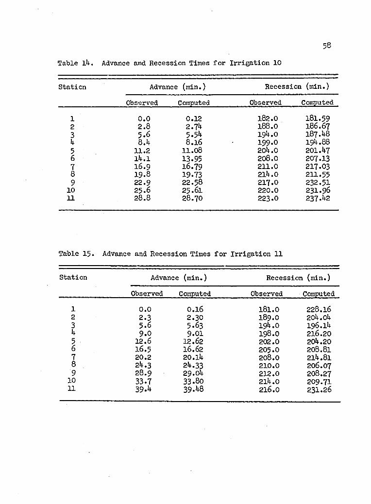
Tables 12, 13, 14, and 15 show both the observed and computed

times for advance and recession. For all irrigations the computed and

observed advance times compare very favorably. The computed and ob­

served recession times for Irrigations 9 and 10 compare reasonably well.

However, the computed and observed recession times for Irrigations 8

and 11 do not compare well. It must be remembered that during reces­

sion, the rate of flow depth change decreases as the flow depth ap­

proaches zero. Thus a small change in flow depth can cause a 10 to

20 minute change in recession time. Small errors in flow depths can

result from using a border surface elevation that is not correct or

water surface elevation that is in error. The equipment and procedure

used in this study were of insufficient precision to determine accurate

recession times. The advance and recession equations for both the ob­

served and computed values are listed in Table l6.

56

Figure 9, Soil Castings of Station 8 for Irrigation 10

Upper -- BEFORE: tf = 0.0321 % = 0.0^2?

Lower — AFTER: (f - 0.0233 X - 0.0251

57

Table 12. Advance and Recession Times for Irrigation 8

Station Advance (min.) Recession (min.)

Observed Computed Observed Computed

1 0 .0 0.16 183.0 210.692 2 .0 2 .16 188.0 204.023 4.2 4.50 191.0 194.714 7-3 7.64 193.0 198.805 10.8 11.16 195.0 204.296 14.4 • 14.64 197.0 200.937 18.7 19.26 198.0 207.348 23.7 24.18 198.5 211.599 30.2 30.23 199.0 202.52

10 36.2 36.45 199-5 209.0311 44.1 44.68 200.0 195.90

Table 13. Advance and Recession Times for Irrigation 9

Station Advance (min.) Recession (min.)

Observed Computed Observed Computed1 0 .0 0 .11 180.5 200.062 2 .2 2.35 I89.O 197.893 5.2 5.35 193.0 193.964 8.5 8.88 196.0 195.855 12.2 12.48 199.0 199.526 16.3 16.34 202.0 206.647 20.3 20.42 205.0 208.378 24.9 25.11 208.0 209.409 29.9 29.99 210.0 210.49

10 35.0 34.99 212.0 227.1711 4l.O 41.22 214.0 235.87

58

Table l4. Advance and Recession Times for Irrigation 10

Station Advance (min.) Recession (min.)

Observed Computed Observed Computed

1 0 .0 0.12 182.0 181.592 2 .8 2.7k 188.0 186.673 5.6 5.54 194.0 187.484 8.4 8 .16 199.0 194.885 11.2 11.08 204.0 201.476 14.1 13.95 208.0 207.137 16.9 16.79 211.0 217.038 19.8 19.73 214.0 211.559 22.9 22.58 217.0 232.51

10 25 .6 25.61 220.0 231.9611 28 .8 28.70 223.0 237.42

Table 15. Advance and Recession Times for Irrigation 11

Station Advance (min.) Recession (min.)

Observed Computed Observed Computed1 0 .0 0 .16 181.0 228.162 2.3 2 .30 I89.O 204.043 5.6 5.63 194.0 196.144 9.0 9.01 198.0 216.205 12.6 12.62 202.0 204.206 16.5 16.62 205.0 208.817 20.2 20.14 208.0 214.818 24.3 24.33 210.0 206.079 28 .9 29.04 212.0 208.27

10 33.7 33.80 214.0 209.7111 39.4 39.48 216.0 231.26

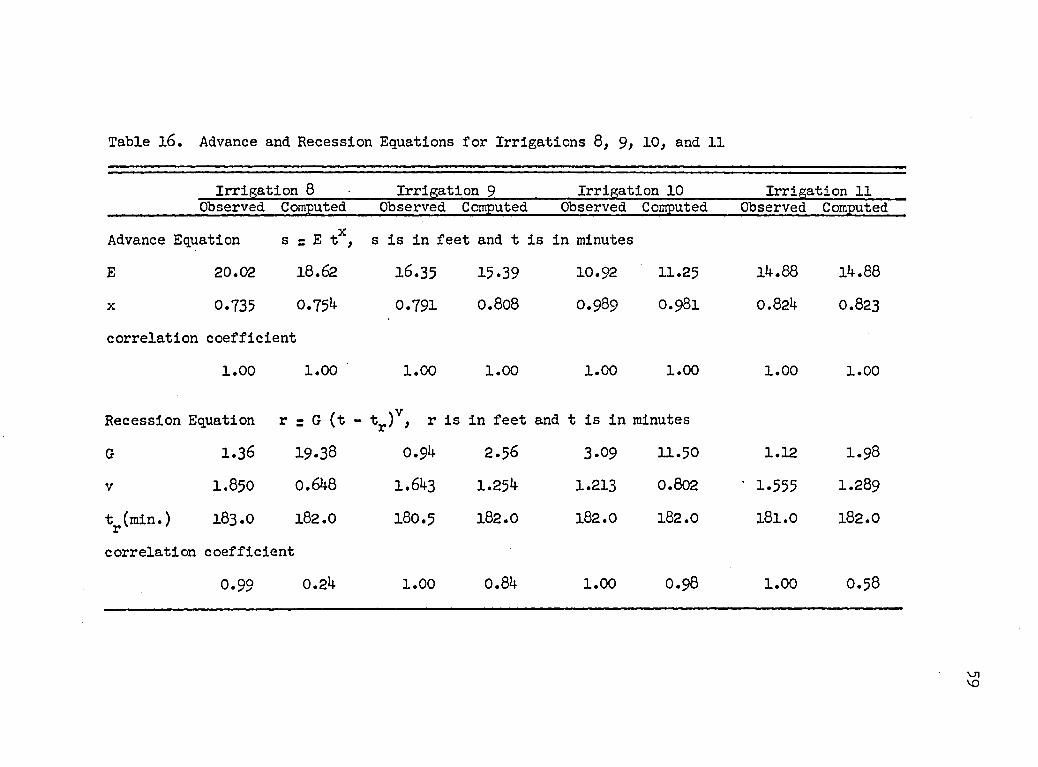
Table l6 . Advance and Recession Equations for Irrigations 8, 9> 10, and 11

Irrigation 8 Irrigation 9 Irrigation 10 Irrigation 11Observed Computed Observed Computed Observed Computed Observed Computed

Advance Equation s = E tX, s is in feet and t :Is in minutes

E 20.02 18.62 16.35 15.39 10.92 11.25 14.88 14.88

x 0.735 0.754 0.791 0.808 O .989 O.98I 0.824 0.823correlation coefficient

1 .00 1.00 1.00 1.00 1.00 1.00 1.00 1.00

Recession Equation r r G (t - tr )v, r is in feet and t is in minutes

G 1 .36 19.38 0.94 2 .56 3.09 11.50 1.12 I .98

v 1.850 0.648 1.643 1.254 1.213 0.802 • 1.555 1.289

tr (min.) 183.O 182.0 180.5 182.0 182.0 182.0 181.0 182.0

correlation coefficient

0.99 0.24 1.00 0.84 1.00 O .98 1.00 O .58

vnVO

CHAPTER 6

DISCUSSION AND CONCLUSIONS

A discussion of variation in roughness with space and time

during border irrigation follows. Effects of flow depth, velocity,

and slope on the computed roughness will be compared. Also the mea­

surement of soil roughness by the soil casts will be compared to the

computed roughness.Even though four different roughness coefficients, Manning,

Sayre-Albertson, Chezy, and Darcy-Weisbach, were computed for differ­

ent times and points along the border, only Manning and Sayre-Albert­

son roughness will be discussed in this chapter. The Manning roughness

coefficient, n, was chosen because of its popularity in design work.

The Sayre-Albertson roughness parameter, % , is discussed because the

computed values can be compared to the measured values. The Chezy,

Darcy-Weisbach, Manning, and Sayre-Albertson equations were related to

each other in equation 10 by using the ratio of the average velocity

to shear velocity

The variations of Manning's n and Sayre-Albertson's X during

Irrigations 8, 9, 10, and 11 are shown in Figures 10, 11, 12, and 13

DiscussionRoughness

60

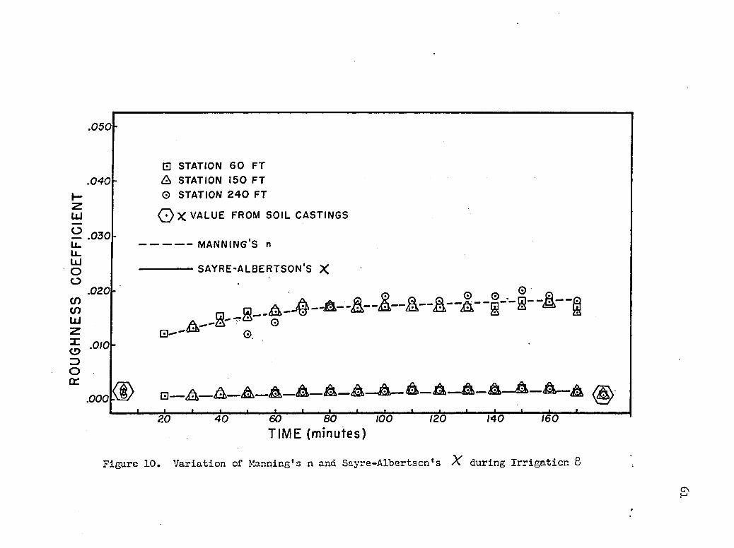
.050

.040-

zUJ— .030 Li_Ll.LUOO

.020 (D CO UJz5 •0 '°ZD O cr

□ STATION 60 FT A STATION 150 FT © STATION 240 FT

(3) X VALUE FROM SOIL CASTINGS

- — —— MANNING'S n

-----------SAYRE-ALBERTSON'S X

n w . A— —A— A A A*""'g ® ^ §

.000 -q_ ^ —A —A —A —A —A —A—A —A —A —A —A—A—A

60 80 100TIME (minutes)

120 140 160

Figure 10. Variation of Manning’s n and Sayre-Albertscn’s X during Irrigation 8

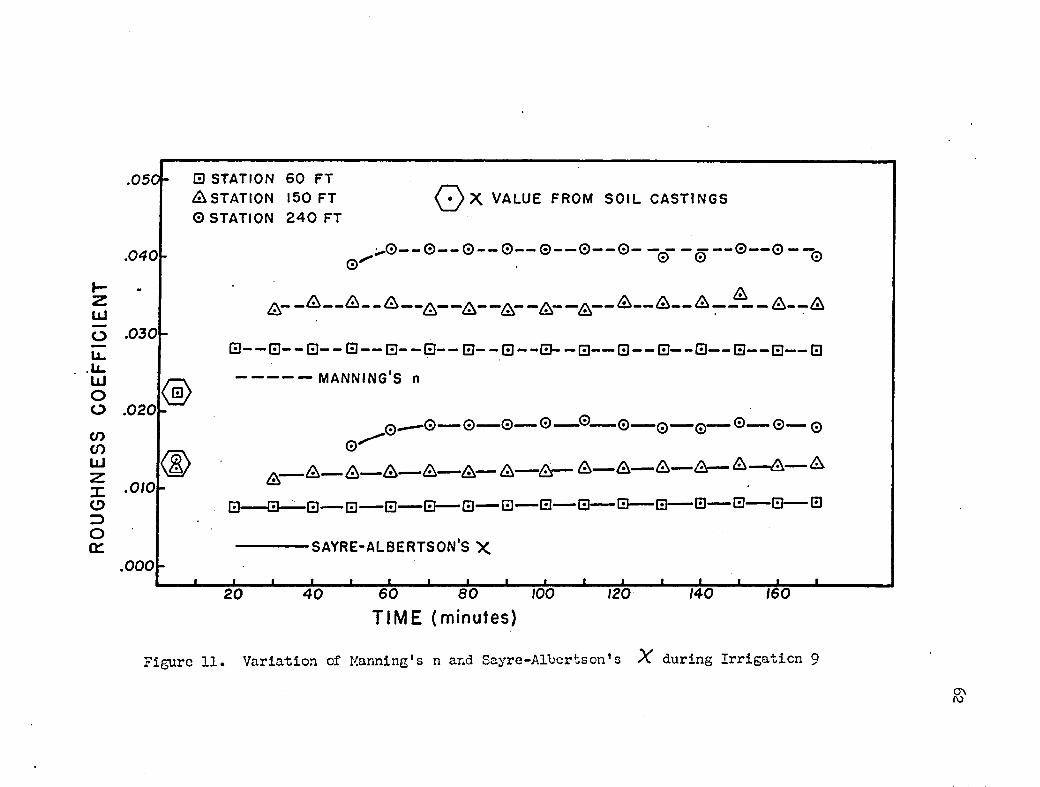
RO

UG

HN

ESS

CO

EFF

ICIE

NT

.0 5 0 -

.0 4 0 -

.0 3 0 -

0 STATION 60 FT A STATION 150 FT G STATION 240 FT

.020-

.0/0

.000 -

<D

i____ I

0 X VALUE FROM SOIL CASTINGS

> © -- O ---© ---© ---© ---© — — © --- - — — =---© -- © ---yo

-A

0-----0-----0-----0-----0-----0-----0- - 0-----0-----0------0-----0------0-----0-----0-----0--------------- MANNING'S n

»©—— © 0 """ © ■ i—® ■■ © ■ ■ Q 1 — Q ' ■ - © — — © ■ ■■ Q

A“ .A_ A— A— A— A— A— A— &— &— &— A— &—A— A.0----- □ ------0------0------0— 0------0— 0— —0— 0— -0— 0------0------0

•SAYRE-ALBERTSON'S X

' ' : ' 1____ |_ 1____ I____ 1 1____ I40 60 80 100

TIME (minutes)120 140 160

Figure 11. Variation of Manning's n and Sayre-Altertson's % during Irrigation 9

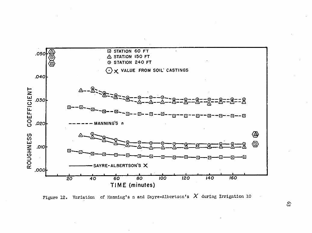
I-zLU

.050

.040

.0 3 0 -

U_U_LUg .020V)</)LUZ .0/0 IoZ)o^ .000

Q STATION 60 FT A STATION 150 FT © STATION 240 FT

( 2 ) X VALUE FROM SOIL' CASTINGS

A — —

0— 0-— 0— 0— 0- . .

- a — A - - A — g = Z @ — g z = & = = g

0 0 — 0 — 0 — — — — n - — m — m —

----------------MANNING'S n

B I3--B--0--0--g--g.---------SAYRE-ALBEHTSON’S X

l:z&=:g=ig=a:&=&=:i ®* 0 — — 0 —— 0 . n — 0 - 0 . . . — 0 i - 0

60 80 100TIME (minutes)

120 140

Figure 12. Variation of Manning’s n and Sayre-Albertsen’s X during Irrigation 10

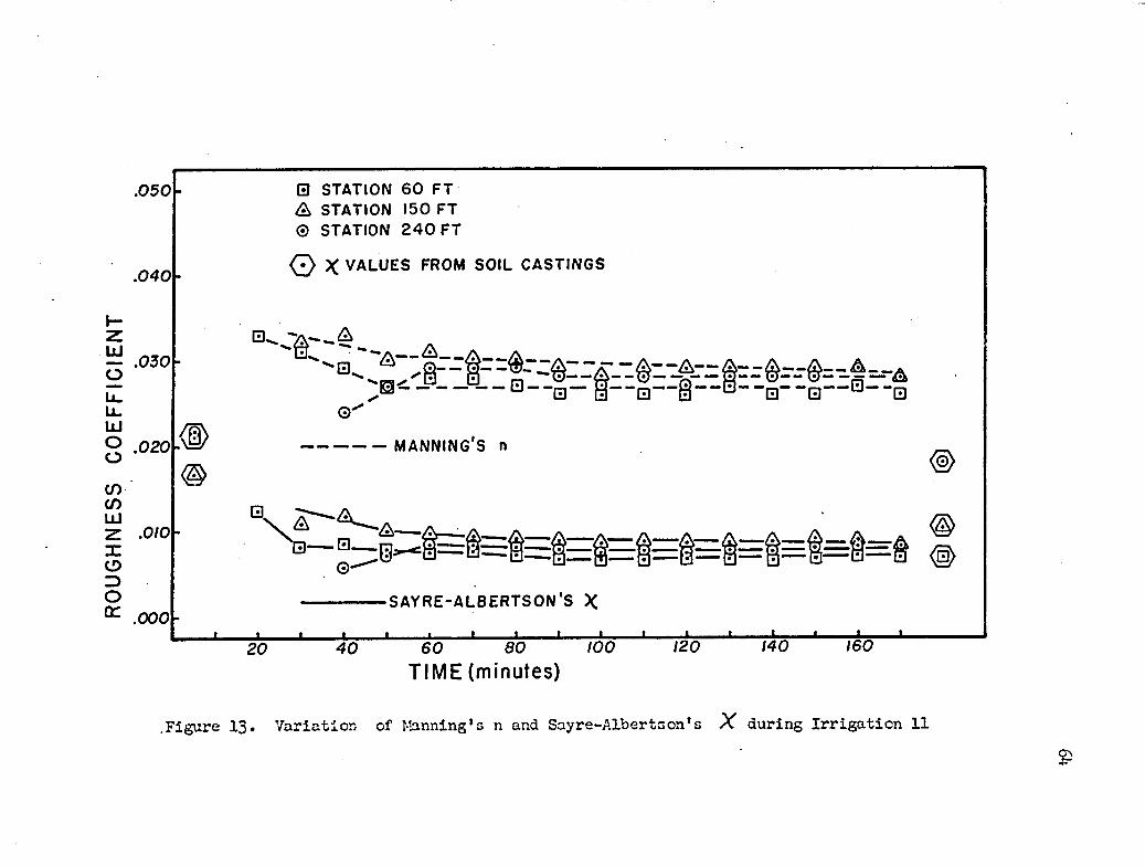
.0 5 0 -

.0 4 0 -

0 STATION 60 FT A STATION 150 FT © STATION 24 0 FT

0 X VALUES FROM SOIL CASTINGS

— .030 OU_U.LUg .020COCOUJzXCD=3Oa:

s.0/0 -

.000 -

' -Q— 0 -- 0 ---0 ---G - - Q - - g ---!ET B"

----------------MANNING'S n

Ns° §=i=:i=i:i=f=i=i=t=S=0 0•SAYRE-ALBERTSON'S X

60 80 100TIME (minutes)

120 140 160

.Figure 13. Variation of Manning’s n and Sayre-Albertson’s % during Irrigation 11

65respectively. The values plotted are the same as those listed in

Tables 28 through 35. Also shown in these figures are the measured X values from the BEFORE and AFTER castings at stations 60 ft., 150 ft.,

and 240 ft. (Table 44). These figures show how roughness varies in

time and space for each irrigation and how the measured X values com­

pare to the computed values.Manning’s n and Sayre-Albertson’s X during Irrigation 8

(Figure 10) did not vary with time or space. The measured X values from the soil castings also closely agree with the computed values and

show that the border was approximately the same roughness before, dur­

ing, and after the irrigation. The Manning n values showed a slight

increase in roughness with time and they do not fit the average line

as well as the computed X values. The average inflow rate during

Irrigation 8 was O .365 c.f.s. and the initial surface roughness was

very smooth, much smoother than normal field conditions. It should

also be remembered that this irrigation does not quite meet Kruse’s

criteria for being classified as a rough boundary because the boundary

condition values were generally less than 0 .52.

The variation of Manning’s n and Sayre-Albertson*s X during Irrigation 9 (Figure 11) differs considerably from Irrigation 8. This

figure shows a definite increase in border roughness with distance.

This is true for both the n and X values. The Sayre-Albertson X values approximately double in value going from station 60 ft. to

station 240 ft. There appears to be no significant change in computed

roughness with time. However, the difference between the measured X values from the BEFORE casts and the first computed X values indicate

that roughness decreased significantly when the soil surface was first

wetted. The computed Sayre-Albertson and Manning values both show the

same trends. The measured X values from the AFTER casts are not

available. Irrigation 9 differed from Irrigation 8 in that the initial

soil surface was rougher and the inflow rate was greater.

Irrigation 10 differs from either of the two previous irriga­

tions discussed because both the inflow rate and initial roughness were

much higher, but is more typical of actual field irrigation. Figure 12

shows the variation of Manning’s n and Sayre-Albertson's X during

Irrigation 10. Roughness appears to change both with time and space.

The changes in roughness with time occur early in the irrigation with

little change 40 minutes after each station was wetted. This is prob­

ably due to the disintegration of the large soil clods. The magnitude

of change between the initial measured X value and the first computed X values for each station is approximately 0.035• The magnitude of

change after the first computed X values is only about 0 .005. Thus

the total X change in time is approximately 0.040.The computed roughness does increase with space. However, the

magnitude difference between stations 150 ft. and 240 ft. is much less

than between stations 60 ft. and 150 ft. This same relationship is

shown by the AFTER casts. The measured X values from the AFTER casts at stations 150 ft. and 240 ft. are nearly the same while the value

from the AFTER cast at station 60 ft. is much less. The X values

from the AFTER casts are larger than the computed X values by approx­imately 0.005. These differences could be caused by using a value for

.66

flow depth, velocity, or slope that is in error. Changes in roughness

due to these factors will he discussed later.Variation in Manning's n and Sayre-Albertson's % during Ir­

rigation 11 are shown in Figure 13. Irrigation 11 is similar to

Irrigation 9, in that the inflow rate and initial soil roughness are

approximately the same. However, the variation of roughness with time

and space of Irrigation 11 is not similar to Irrigation 9« Roughness

during Irrigation 11 does not increase with space as in Irrigation 9*

Roughness for Irrigation 11 does increase between stations 60 ft. and

150 ft. but decreases between stations 150 ft. and 2U0 ft. The mea­

sured values of X from the AFTER castings show a consistent increas­ing trend in roughness from stations 60 ft. to 240 ft. The measured

X value for station 60 ft. agrees with the computed X values for station 60 ft. but measured X values for stations 150 ft. and 240 ft.

are greater than the computed values.

There appears to be no trend of roughness variation with time

for Irrigation 11. Stations 60 ft. and 150 ft. show a slight decrease

in roughness with time during the first 40 minutes they were wetted,

and then roughness remains constant with time. Station 240 ft. shows

an increase in roughness during the first 20 minutes after wetting and

then remains constant. The difference between the measured X values from the BEFORE and AFTER castings indicate that roughness should have

decreased with time. Both Manning's n and Sayre-Albertson's X show the same trend of roughness variation in time and space.

The computed X values for Irrigations 9 and 10 show a con­

sistent trend of increasing roughness with increasing distance along

67

.68

the border. Irrigation 8 shows no trend of increasing roughness with

distance and Irrigation 11 shows an increase and then a decrease in

computed X roughness with distance. These four irrigations do not

show any consistent % roughness change with distance.

Measured changes in X roughness due to distance can also be shown by the BEFORE and AFTER castings. Eleven irrigations were con­

ducted for this study, even though the hydraulic data from the first

seven irrigations were not used, the soil castings were valid for com­

paring measured X roughness changes. Table 17 is a summary of Irri­

gations 1 through 7» All irrigations except Irrigation 6, were

conducted on a tilled surface. Irrigation 6 was conducted the day

after Irrigation 5, thus the surface condition of Irrigation 6 was

established by Irrigation $. The duration of inflow for Irrigations

1 through 4 was between 30 and 60 minutes, and for Irrigations 5, 6,

and 7 it was between 100 and 125 minutes.

Measured Sayre-Albertson's X from the BEFORE casts (Figure 14) shows the X values for stations 60 ft., 150 ft., and 240 ft.

for all eleven irrigations. This bar graph shows that the initial

soil roughness is quite random. No one station is always rougher or

smoother than the other two stations.

If the roughness along the border is varying with space it

should be shown by the AFTER castings. Measured Sayre-Albertson*s X from the AFTER castings (Figure 15) shows the X values for stations 60 ft., 150 ft., and 240 ft. for all irrigations except Irrigation 9*

Irrigations 3; 6, 7# 8, 10, and 11 indicate that roughness increased

with distance down the border. Irrigations 1, 2, and 4 show that

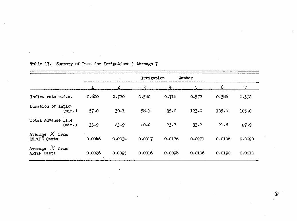
Table 17. Summary of Data for Irrigations 1 through 7

Irrigation Number

1 2 3 4 5 6 7Inflow rate c.f.s. 0.600 0.720 0.580 0.718 0.572 0.386 0.392Duration of inflow

(min.) 57.0 30.1 58.1 35 .0 123.0 105.0 105.0

Total Advance Time(min.) 33-9 23 .9 20.0 23 .7 33.2 21.8 27.9

Average X from BEFORE Casts 0.0046 0.0034 0.0017 0.0176 0.0271 0.0106 0.0020

Average X from AFTER Casts 0.0026 0.0025 0.0016 0.0098 0.0106 0.0190 0.0013

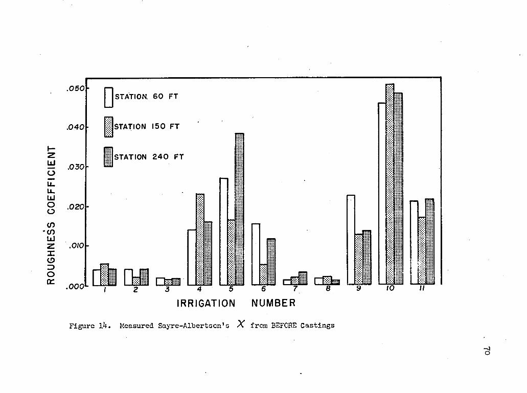
STATION. 60 FT

STATION 150 FT

STATION 2 4 0 FT

IRRIGATION NUMBER

. Measured Sayre-Albertscn’s % from BEFORE CastingsFigure 14

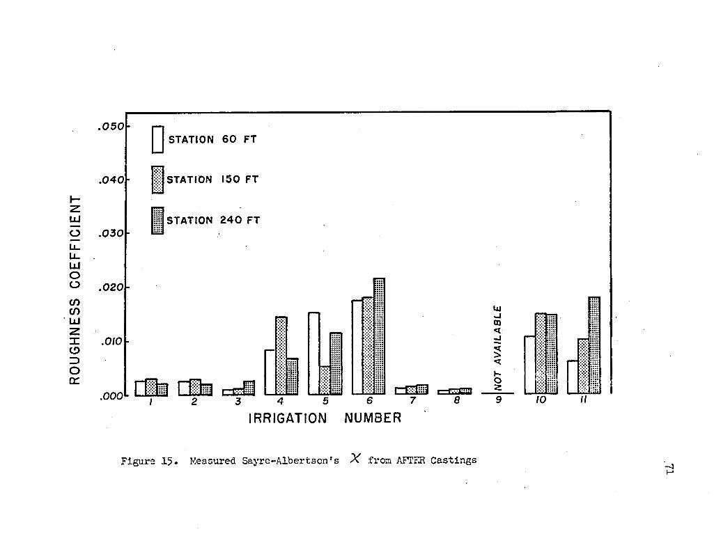
.050STATION 60 FT

STATION ISO FT

STATION 24 0 FT.030

IRRIGATION NUMBER

Figure 15. Measured Sayre-Albertson’s % from AFTER Castings

roughness increased from station 60 ft. to station 150 ft. but then

decreased going down the border. Again there is no consistent trend

of soil roughness with space.The pattern of variation of roughness along the border is not

consistent between the BEFORE and AFTER castings. For example the

BEFORE castings of Irrigation 11 (Figure l4) show that stations 60 ft.

and 240 ft. are approximately the same roughness, while station 150 ft.

is much less. However the AFTER castings (Figure 15) show that rough­

ness increases with distance along the border. Irrigations 2, 3* 4,

5, 6, and 8 also indicate that the pattern of variation of roughness

is not consistent.

The change of roughness due to time can be shewn by comparing

the average measured % values from the BEFORE and AFTER castings.

In Figure l6 the average Sayre-Albertson’s % from the BEFORE and

AFTER castings are shown for all eleven irrigations. All irrigations,

except Irrigation 6, show that the measured X roughness decreased

during the irrigation. Since all these irrigations were conducted on

freshly tilled soil, the decrease in roughness is probably due to the

disintegration of the soil clods. Irrigation 6 was conducted on the

freshly wetted soil of Irrigation 5»

Flow rate might be expected to cause a change in roughness.

Comparing Irrigations 2 and 4, the inflow rates for both were 0.72

c.f.s. but the initial soil roughness was different. Both irrigations

have equal inflow durations. However, the change in roughness between

the two was different. The roughness for Irrigation 2 did not change

significantly between the measured X values from the BEFORE and AFTER

72

.050BEFORE CASTINGS

AFTER CASTINGS

IRRIGATION NUMBER

Figure l6. Average Sayre-Albertscn's % from BEFORE and AFTER Castings

lh

casts but % values for Irrigation 4 reduced by one-half. Also the

measured % roughnesses from the AFTER castings for Irrigations 2 and

4 are not equal. This may suggest that there is not necessarily a

regime roughness associated with each flow rate, but that perhaps the

initial soil roughness influences the final soil roughness more than

the flow rate. Irrigations 6 and 7 can be similarly analyzed. How­

ever the conclusion from Irrigations 6 and 7 is that roughness decreased

for Irrigation 7 but roughness increased for Irrigation 6 . These two

irrigations also hint that there is not necessarily a regime roughness

resulting from a given flow rate.

Effects of ParametersAs was mentioned previously, errors in the measurement of the

parameters, flow depth, velocity, and slope, could cause errors in the

computed values of Manning's n and Sayre-Albertson's X . The Manning

and Sayre-Albertson equations (equations 6 and 18 respectively) both

include the parameters of velocity, slope, and hydraulic radius. The

Sayre-Albertson equation also includes flow depth. For wide, shallow

flow the hydraulic radius approximately equals the flow depth.

When the error causes the measured depth to be less than its

actual value, the computed roughness will also be less than its actual

value if slope and velocity remain constant. The opposite happens

when the error causes increases in flow depths. Errors in the computed

roughness values would also occur if the values for velocity were in

error. As was described in Chapter 4, velocities were determined by

equation 26, an equation of continuity. An accurate solution of this

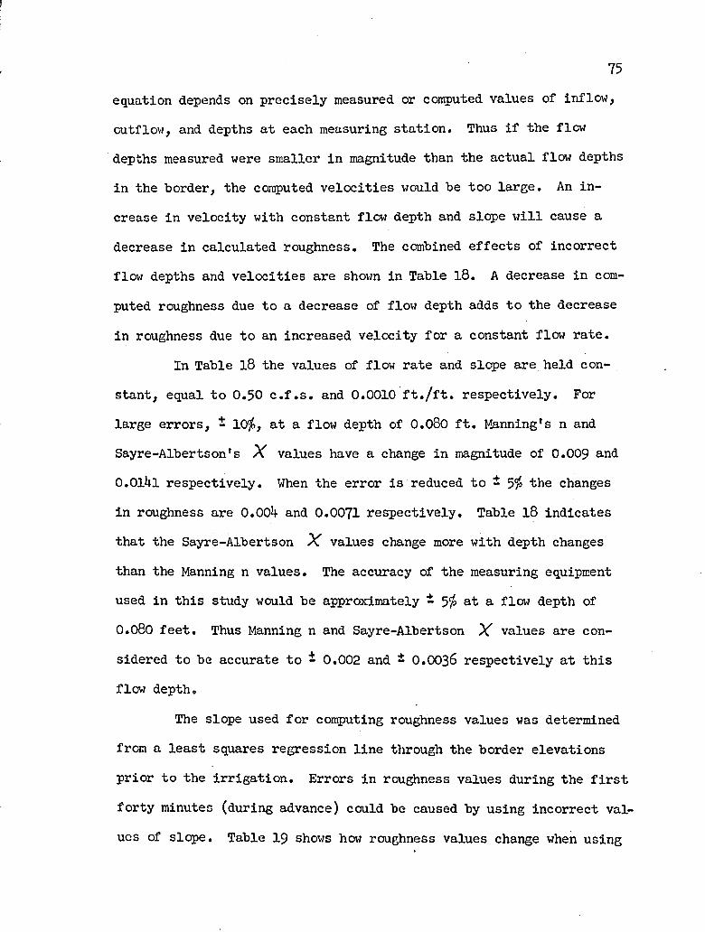
75

equation depends on precisely measured or computed values of inflow,

outflow, and depths at each measuring station. Thus if the flow

depths measured were smaller in magnitude than the actual flow depths

in the border, the computed velocities would be too large. An in­

crease in velocity with constant flow depth and slope will cause a

decrease in calculated roughness. The combined effects of incorrect

flow depths and velocities are shown in Table 18. A decrease in com­

puted roughness due to a decrease of flow depth adds to the decrease

in roughness due to an increased velocity for a constant flow rate.

In Table 18 the values of flow rate and slope are held con­

stant, equal to 0.50 c.f.s. and 0.0010 ft./ft. respectively. For

large errors, - 10$, at a flow depth of 0.080 ft. Manning's n and

Sayre-Albertson's X values have a change in magnitude of 0.009 and

O.OlUl respectively. When the error is reduced to - 5$ the changes

in roughness are 0.004 and 0.0071 respectively. Table 18 indicates

that the Sayre-Albertson X values change more with depth changes than the Manning n values. The accuracy of the measuring equipment

used in this study would be approximately - 5$ at a flow depth of

0.080 feet. Thus Manning n and Sayre-Albertson X values are con­

sidered to be accurate to - 0.002 and - O.OO36 respectively at this flow depth.

The slope used for computing roughness values was determined

from a least squares regression line through the border elevations

prior to the irrigation. Errors in roughness values during the first

forty minutes (during advance) could be caused by using incorrect val­

ues of slope. Table 19 shows how roughness values change when using

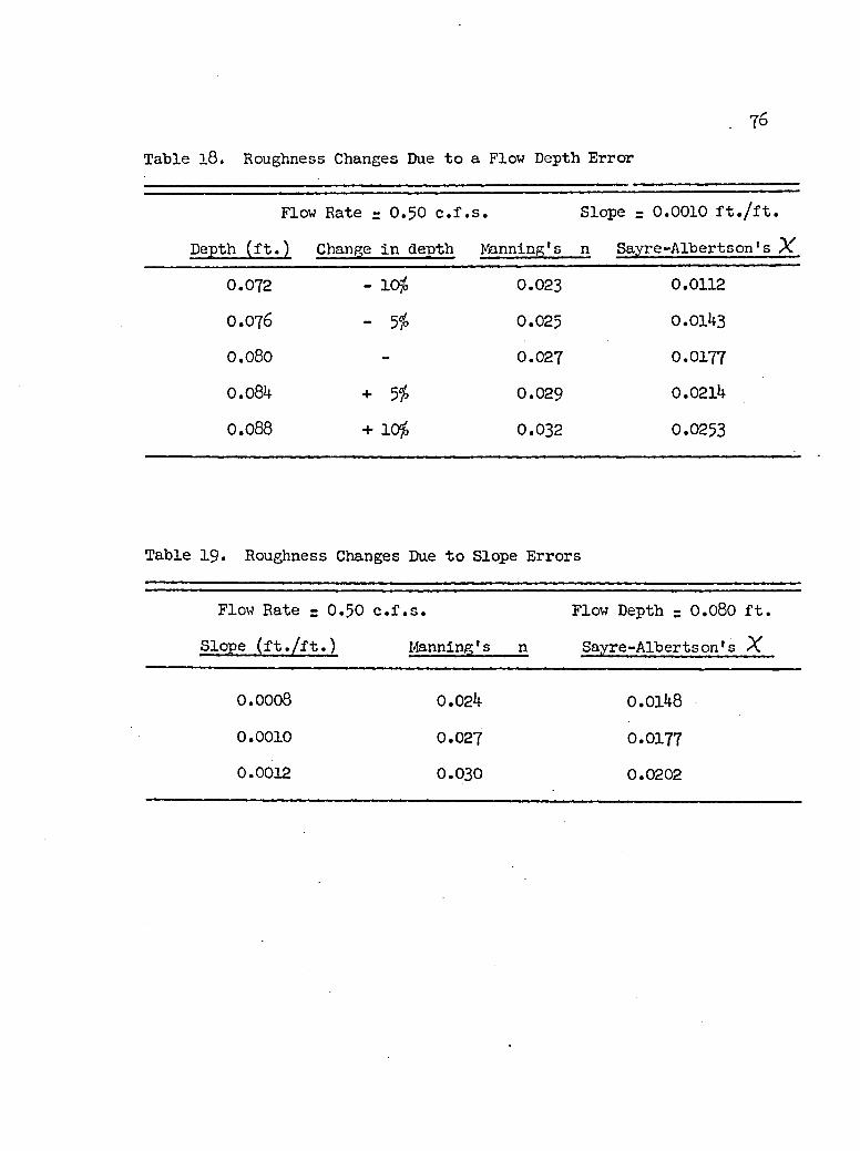
76

Table l8. Roughness Changes Due to a Flow Depth Error

Depth (ft.

Flow Rate = 0.50 c.f.

,) Change in depth

,s.

Manning's

Slope % 0.0010 ft./ft.

n Sayre-Albertson's %

0.072 - H # 0.023 0.0112

0.076 - % 0.025 0.0143

0.080 - 0.027 0.01770.084 + % 0.029 0.0214

0.088 + M # 0.032 0.0253

Table 19. Roughness Changes Due to Slope Errors

Flow Rate z 0.50 c.f.s. Flow Depth z 0.080 ft

Slope (ft./ft.) Manning's n Sayre-Albertson's X

0.0008 0.024 0.01480.0010 0.027 0.01770.0012 0.030 0.0202

77an improper slope. By using a constant slope of 0.0010 ft./ft.,

Manning’s n and Sayre-Albertson's X values can both vary * 0.003 if

the slope used was 0.0010 and it should have been 0.0008 or 0 .0012.

These are the maximum deviations shown in Table 11. Errors of improper

slope would also combine with errors in roughness caused by incorrect

flow depths and velocities.At first glance one might expect the Sayre-Albertson equation

to be less accurate than Manning’s equation because of the larger

changes in Sayre-Albertson’s X compared to Manning's n due to mea­

surement errors of the parameters, flow depth, velocity, and slope.

If the Manning and Sayre-Albertson equations (equations 6 and l8 re­

spectively) were used to determine either velocity, flow depth, or

slope, more care must be exercised in selecting a Manning n value than

a Sayre-Albertson X value to obtain the same accuracy. This indi­

cates that the Sayre-Albertson equation is more applicable to border

irrigation because the Sayre-Albertson X values need not be of the

same accuracy as Manning n values and the Sayre-Albertson X values are also related to statistical soil roughness measurements.

Conclusions

It is impossible to draw any general conclusions from the four

irrigations used as to whether the roughness during border irrigation

varies with time or space. Obviously more irrigations are needed.

Analysis of the data in this study does suggest some relationships:

1. Roughness decreases with time for all irrigations conducted

on tilled soil. This decrease occurs within the first few

minutes of wetting and is probably due to disintegrating

of the soil clods.2. There appears to be no particular roughness resulting from

a given flow rate, but perhaps the initial soil roughness

influences the final roughness for each flow rate.

3. Roughness does not necessarily increase with increasing

distance as was shown by Irrigations 9 and 10. Roughness

may increase and then decrease or it may remain constant

as shown by Irrigations 11 and 8 respectively.

4. The measured values of Sayre-Albertson's % from soil

castings give reasonable agreement with the computed values

of Sayre-Albertson's X .

As was mentioned previously, more irrigations are needed to

evaluate the changes of roughness during border irrigation. These

irrigations should be at various slopes, roughnesses, and inflow

rates. These tests should not only be conducted on tilled soil, but

also several irrigations should be made between tillings. The irriga­

tions could also be extended to borders with vegetation.

The irrigations also provide accurate data which can be used

to validate mathematical models simulating border irrigations. Be­

cause of the tremendous amount of labor and time involved in collect­

ing field data, it is much easier to simulate irrigations by using

78

such models

APPENDIX A

DETERMINATION OF FLOW REGIME

79

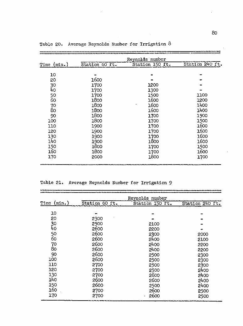
80Table 20. Average Reynolds Number for Irrigation 8

Time (min.)Reynolds number

Station 6o ft. Station 150 ft. Station 240 ft.

1020 1600 - -30 1700 1200 -40 1700 1300 -50 1700 1500 110060 1800 1600 120070 1800 1600 i4oo80 1800 1600 l4oo90 1800 1700 1500

100 1800 1700 1500no 1900 1700 1600120 1900 1700 1600130 1900 1700 1600i4o 1900 1800 1600150 1800 1700 1500160 1800 1700 1600170 2000 1800 1700

Table 21. Average Reynolds Number for Irrigation 9

Time (rain.)Reynolds number

Station 60 ft. Station 150 ft. Station 240 ft.10 - - -20 2300 - -30 2500 2100 -40 2600 2200 -50 2600 2300 200060 2600 2400 210070 2600 2400 220080 2600 2400 220090 2600 2500 2300

100 2600 2500 2300no 2700 2500 2300120 2700 2500 2400130 2700 2600 2400i4o 2600 2600 2400150 2600 2500 2400160 2700 2600 2500170 2700 • 2600 2500

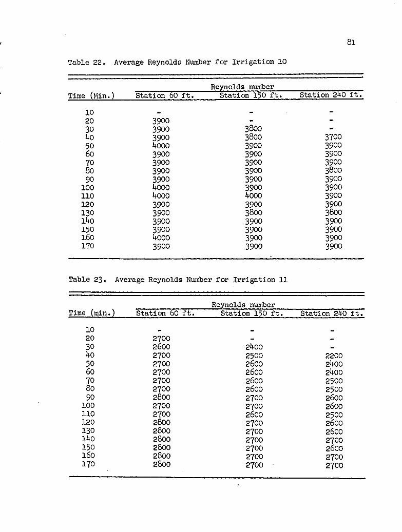
81

Table 22. Average Reynolds Number for Irrigation 10

Reynolds numberTime (Min.) Station 60 ft. Station 150 ft. Station 240 ft.

10 - - -20 3900 — -30 3900 3800 —ho 3900 3800 370050 4000 3900 390060 3900 3900 390070 3900 3900 390080 3900 3900 380090 3900 3900 3900

100 4000 3900 3900110 4ooo 4000 3900120 3900 3900 3900130 3900 3800 3800i4o 3900 3900 3900150 3900 3900 3900l 6o 4000 3900 3900170 3900 3900 3900

Table 23. Average Reynolds Number for Irrigation 11

Reynolds numberTime (min.) Station 60 ft. Station 150 ft. Station 240 ft.

10 _

20 2700 - -30 2600 2400 -40 2700 2500 220050 2700 2600 240060 2700 2600 240070 2700 2600 250080 2700 2600 250090 2800 2700 2600

100 2700 2700 2600110 2700 2600 2500120 2800 2700 2600130 2800 2700 2600l 4o 2800 2700 2700150 2800 2700 2600160 2800 2700 2700170 2800 2700 2700

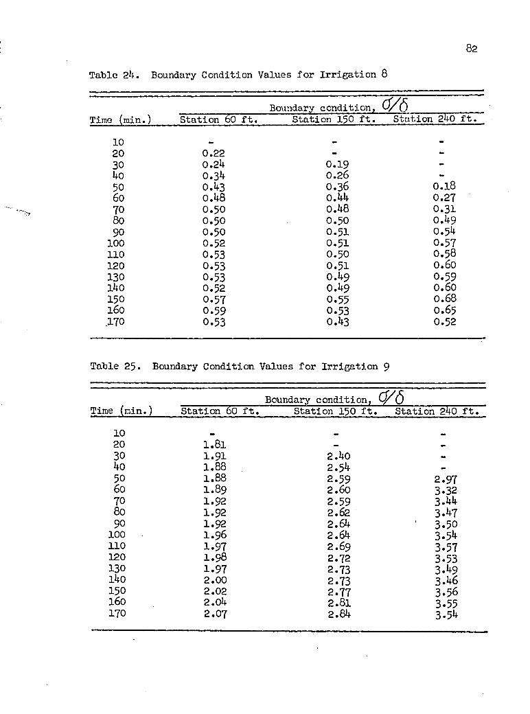
82Table 24. Boundary Condition Values for Irrigation 8

Time (min.)Boundary condition. 0/6

Station 6o ft. Station 150 ft. Station 240 ft.

1020 0.22 - -30 0.24 0.19 -40 0.34 0.26 -50 0.43 0.36 0.1860 0.48 0.44 0.27?o 0.50 0.48 0.3180 0.50 0.50 0.4990 0.50 0 .51 0.54

100 0.52 0 .51 0.57110 0.53 0.50 0.58120 0.53 0.51 0.60130 0.53 0 .49 0.59140 0.52 0.49 0.60150 0.57 0.55 0.68l 6o 0.59 0.53 0.65.170 0.53 0.43 0.52

Table 25• Boundary Condition Values for Irrigation 9

Time (min.)Boundary condition, (^(5

Station 60 ft. Station 150 ft. Station 240 ft.1020 1 .81 - -

30 1.91 2.40 -

40 1.88 2.54 -

50 1.88 2.59 2.9760 I .89 2 .60 3.3270 1.92 2.59 3.4480 1.92 2.62 3.4790 1.92 2.64 ' 3.50

100 1.96 2.64 3.54110 1.97 2 .69 3.57120 1 .98 2.72 3.53130 1.97 2.73 3.49i 4o 2 .00 2.73 3.46150 2.02 2.77 3.56160 2.04 2 .81 3.55170 2 .07 2.84 3.54

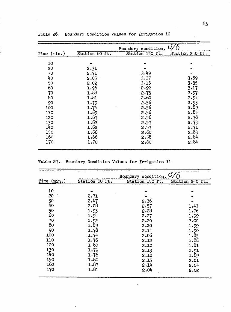
83

Table 26. Boundary Condition Values for Irrigation 10

Time (min.)Boundary condition, 6

Station 60 ft. Station 150 ft. Station 240 ft.

1020 2.31 - -30 2.71 3.49 -ko 2.05 ' 3.37 3-5950 2.02 3.15 3.356o 1.96 2.92 3.1770 1.88 2.73 2.9780 1.81 2 .60 2.9490 1.79 2.56 2.93

100 1.74 2 .56 2 .89110 1.69 2 .56 2.84120 1.67 2 .56 2 .78130 1.62 2.57 2.73140 1.62 2.57 2.71150 1.66 2 .60 2.83160 1.66 2 .58 2.84170 1.70 2 .60 2.84

Table 2?. Boundary Condition Values for Irrigation 11

Boundary condition,Time (min.) Station 60 ft. Station 150 ft. Station 240 ft.

10 _20 ' 2.71 - -30 2.47 2.36 -4o 2.08 2.57 1.4350 1.93 2.28 1.7660 1.94 2.27 1.9970 1.92 2.20 2.0080 1.89 2.20 1.9990 1.78 2.14 1.90

100 1.74 2 .06 1.85110 1.76 2.12 1.86120 1.80 2.10 l .8l130 1.79 2.13 1.91l4o 1 .76 2.10 1.89150 1.80 2.15 2.01160 1.87 2.14 2.04170 1 .8l 2.04 2.02

APPENDIX B

COMPUTED VALUES OF MANNING, SAYRE-ALBERTSON, CHEZY, AND DARCY-V/EISBACH ROUGHNESSES

AND MEASURED X VALUES

84

85Table 28. Computed Values of Manning's n for Irrigation 8

Manning's nTime (min.) Station 60 ft. Station 150 ft. Station 240 ft.

10 - - -20 0.012 - -30 0.013 0.013 -40 0.015 0.014 -50 0.016 0.015 0.01260 0.016 0.016 0.01470 0.017 0.017 0.0168o 0.017 0.017 0.01790 0.017 0.017 0.018

100 0.017 0.017 0.019110 0.017 0.017 0.018120 0.017 0.017 0.018130 0.017 0.017 0.019l4o 0.017 0.016 0.019150 0.018 ' 0.017 0.020160 0.018 0.018 0.019170 0.017 0.016 0.018

Table 29. Computed Values of Manning's n for Irrigation 9

Time (min.)Manning's n

Station 60 ft. Station 150 ft. Station 240 ft.1020 0.028 -30 0.028 0.033 -4o 0.028 0.034 -50 0.028 0.034 0.03960 0.028 0.034 0 .04l70 0.028 0.033 o.o4i80 0.028 0.033 o.o4i90 0.028 0.033 o.o4i

100 0.028 0.033 o.o4i110 0.028 0.033 o.o4i120 0.028 0.034 o.o4i130 0.028 0.034 o.o4o140 0.028 0.034 o.o4o150 0.028 0.035 0.041160 0.028 0.034 0.041170 0.028 0.034 o.o4o

86

Table 30. Computed Values of Manning's n for Irrigation 10

Time (min.)Manning's n

Station 60 ft. Station 150 ft. Station 240 ft.

10 ■

20 0.027 - -30 0.027 0.034 -1*0 0.026 0.034 0.03550 0.025 0.032 0.0336o 0.025 0.031 0.03270 0.024 0.030 0.0318o 0.024 0.029 0.03190 0.024 0.029 0.031

100 0.024 0.029 0.031110 0.023 0.029 0.030120 0.023 0.029 0.030130 0.023 0.029 0.030i 4o 0.023 0.028 0.030150 0.023 0.029 0.030160 0.023 0.029 0.030170 0.023 0.029 0.030

Table 31• Computed Values of Manning's n for Irrigation 11

________ Manning's n___________________________ ______Time (min.)_____Station 60 ft. Station 150 ft. Station 240 ft.

10 - - -20 0.033 - -30 0.031 0.032 -4o 0.029 0.033 0.02450 0.027 0.030 0.02760 0.028 0.031 0.02970 0.028 0.030 0.02980 0.027 0.030 0.02990 0.026 0.029 0.028100 0.026 0.028 0.027110 0.026 0.029 0.028120 0.026 0.029 0.027130 0.027 0.029 0.028

140 0.026 0.029 0.028150 0.026 0.029 0.028160 0.027 0.029 0.029170 0.026 0.028 0.028

87

Table 32. Computed Values of Sayre-Albertson's X for Irrigation 8

Time (min.)Sayre-Albertson's X

Station 60 ft. Station 150 ft. Station 240 ft.

1020 0.0005 - -30 0.0005 o.ooo4 -40 0.0009 0.0006 -50 • 0.0012 0.0010 o.ooo46o 0.0013 0.0012 0.000770 0.0014 0.0014 0.00128o 0.0014 0.0015 0.001490 0.0014 0.0015 0.0017

100 0.0015 0.0015 0.0018110 0.0015 0.0015 0.0018120 0.0015 0.0015 0.0019130 0.0015 0.0015 0.0019140 0.0015 0.0014 0.0019150 0.0018 0.0017 0.0023160 0.0018 0.0016 0.0022170 0.0014 0.0012 0.0015

Table 33• Computed Values of Sayre-Albertson's X for Irrigation 9

Time (min.)Sayre-Albertson's X

Station 60 ft. Station 150 ft. Station 240 ft.1020 0.0074 - -30 0.0077 0.0112 -4o 0.0075 0.0120 -50 0.0075 0.0121 0.015460 0.0075 0.0121 0.017570 0.0077 0.0120 0.018180 0.0077 0.0121 0.018290 0.0076 0.0122 0.0184

100 0.0079 0.0122 0.0185110 0.0079 0.0125 0.0187120 0.0080 0.0126 0.0182130 0.0078 0.0126 0.0179140 0.0080 0.0126 0.0177150 O.OO83 0.0130 0.0185160 0.0082 0.0130 0.0183170 O.OO83 0.0132 0.0180

88Table 34. Computed Values of Sayre-Albertson's X for Irrigation 10

Time (min.)Sayre-Albertson's X

Station 6o ft. Station 150 ft. Station 240 ft.

10 _

20 0.0083 - -

30 0.0076 0.0147 -40 0.0070 0.0140 0.015450 0.0068 0.0127 0.013760 O.OO65 0.0113 0.012670 0.0062 o.oio4 0.01168o 0.0058 0.0097 0.011690 0.0057 0.0094 o.on4

100 0.0055 0.0094 0.0112110 0.0052 0.0094 0.0109120 0.0052 0.0095 0.0106130 0.0050 0.0096 0.0104l4o 0.0050 0.0095 0.0103150 0.0052 0.0097 0.0109160 0.0051 0.0096 0.0109170 0.0054 0.0097 0.0110

Table 35• Computed Values of Sayre-Albertson* s X for Irrigation 11

Time (min.)Sayre-Albertson's X

Station 60 ft. Station 150 ft. Station 240 ft.1020 0.0123 - -

30 0.008l 0.0107 -40 0.0085 0.0117 0.005750 0.0076 0.0098 0.007160 0.0076 0.0097 O.OO8370 0.0076 0.0093 O.OO8380 0.0074 0.0092 O.OO8290 O.OO67 0.0088 O.OO76

100 0.0066 • 0.0084 0.0073110 0.0067 O.OO87 0.0075120 0.0068 O.OO85 0.0070130 0.0068 0.0088 O.OO76l4o 0.0066 0.0086 O.OO75150 0.0068 0.0088 0.00S1160 0.0073 0.0088 0.0083170 O.OO69 0.0082 0.0082

89

Table 36. Computed Values of Chezy's C for Irrigation 8

Chezy1s CTime (min.) Station 60 ft. Station 156 ft. Station 240 ft.

10 - - -20 72 - -30 68 69 ■ -40 62 64 -50 57 58 6960 56 55 6270 55 53 5480 55 53 5190 55 53 50

100 54 53 49110 54 53 49120 53 53 48130 54 54 49i4o 54 54 49150 52 52 47160 52 52 47170 55 57 52

Table 37• Computed Values of Chezy's C for Irrigation 9

Chezy1s CTime (min.) Station 60 ft. Station 150 ft. Station 240 ft.

10 _

20 35 - -

30 35 29 *»

4o 35 29 -

50 36 29 2560 35 29 2470 35 30 2480 35 • 29 2490 35 30 24

100 35 30 24110 34 29 24120 34 29 25130 35 29 25l 4o 34 29 25150 34 29 24160 34 29 25170 34 29 25

90

Table 38. Computed Values of Chezy's C for Irrigation 10

Chezy’s CTime (min.) Station GO ft. Station 150 ft. Station 2k0 ft.

10 - - -20 37 - -30 38 30 -4o 40 31 3050 39 32 3160 40 34 3270 41 34 3380 42 35 3390 42 35 33

100 42 35 33110 43 35 34120 43 35 34130 43 35 34140 43 35 34150 43 35 33160 43 35 34170 43 35 34

Table 39. Computed Values of Chezy1's C for Irrigation 11

Time (min.)Chezy1s C

Station 60 ft. Station 150 ft. Station 240 ft.10 — - -20 30 - -30 31 32 -4o 34 30 4l50 36 32 3660 36 33 3470 35 33 3480 36 33 3490 37 34 35100 37 34 36110 37 33 35120 37 34 36130 37 34 35l 4o 37 33 36

150 37 34 34160 36 34 34170 37 34 34

91

Table 40. Computed Values of Darcy-Weisbach * s f for Irrigation 8

Darcy-Weisbach’s fTime (min.) Station 60 ft. Station 150 ft . Station 240 ft.

1020 0.055 - -30 0.058 0.057 -4o 0.071 0.066 -50 0.083 0.079 0.0576o O.O87 0.088 0.070TO O.O89 0.093 0.0918o O.O89 0.095 0.10090 0.090 0.095 0.106

100 0.092 0.095 0.109110 0.093 0.093 0.109120 0.093 0.093 0.110130 0.092 0.091 0.109l4o 0.091 0.090 0.109150 0.102 0.101 0.122160 0.102 0.099 0.119170 0.088 0.081 0.096

Table 4l. Computed Values of Darcy-Weisbach1s f for Irrigation 9

Darcy-Weisbach*s fTime (min.) Station 6 0 ft. Station 150 ft. Station 240 ft.

10 _ _

20 0.215 - mm

30 0.216 0.307 -40 0.211 0.315 -50 0.209 0.311 0.41360 0.208 0.305 0.44470 0.211 0.301 0.44880 0.212 0.304 0.44790 0.210 0.304 0.444

100 0.214 ■ 0.301 0.443no 0.214 0.306 0.444120 0.215 0.307 0.428130 0.211 0.304 0.417l4o 0.217 0.305 0.412150 0.221 0.316 0.435160 0.217 0.310 0.423170 0.220 0.312 0.410

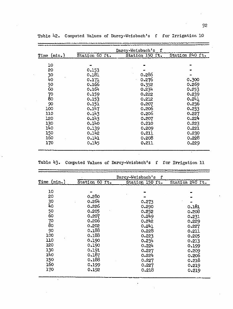
Table 42. Computed Values of Darcy-Weisbach’s f for Irrigation 10

Darcy-Weisbach*s fTime (min.) Station 60 ft. Station 150 ft. Station 240 ft.

10 _

20 0.153 - -30 0 .l8l 0.286 -40 0.171 0.276 0.30050 0.166 0.352 0.26960 0.164 0.234 0.25370 0.159 0.222 0.23980 0.153 0.212 0.24190 0.151 0.207 0.236

100 0.147 0.206 0.233110 0.143 0.206 0.227120 0.143 0.207 0.224130 o.i4o 0.210 0.223i4o 0.139 0.209 0.221150 0.142 0.211 0.230160 0.l4l 0.208 0.228170 0.145 0.211 0.229

Table 43. Computed Values of Darcy-Weisbach's f for Irrigation 11

Darcy-Weisbach1s fTime (min.) Station 60 ft. Station 150 ft * Station 240 ft.

1020 0.280 -30 0.264 0.273 -4o 0.226 0.290 0.18150 0.205 0.252 0.20860 0.207 0.249 0.23170 0.206 0.242 0.22980 0.202 0.241 0.22790 0.188 0.228 0.211

100 0.188 0.223 0.205110 0.190 0.234 0.213120 0.190 0.224 0.199130 0.191 0.227 0.209l4o 0.187 0.224 0.206150 0.188 0.227 0.218160 0.199 0.227 0.219170 0.192 0.218 0.219

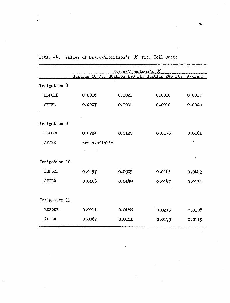
93

Table 44. Values of Sayre-Albertson's X from Soil Casts

Sayre-Albertson’s XStation 60 ft. Station 150 ft. Station 240 ft. Average

Irrigation 8

BEFORE 0.0016 0.0020 0.0010 0.0015AFTER 0.0007 0.0008 0.0010 0.0008

Irrigation 9

BEFORE 0.0224 0.0125 0.0136 0.0161

AFTER not available

Irrigation 10

BEFORE 0.0457 0.0505 0.0483 0.0482AFTER 0.0106 0.0149 0.0147 0.0134

Irrigation 11

BEFORE 0.0211 0.0168 0.0215 0.0198

AFTER 0.0067 0.0101 0.0179 0.0115

94

Symbol Dimensions

LIST OF SYMBOLS

Description

a - Constant .

A L2 Area of flow cross section

Ar - Constant

As - Constant

Aw - Constant

B1- Constant

B2 ~ Constant

B3- Constant

B4 - Constant

B5 - Constant

b6 - Constant

C L Distance from the trolley to casting top

C - Resistance coefficient from Chezy's equation

d L Depth of flow

dIi,j L3 Volume infiltrated in reach i during period j

49i,j L3 Volume of inflow into reach i during period j

as. i3 Volume of surface storage in reach i duringJ period j

e - Base of Naperian logarithm

E - Constant

f - Friction factor from Darcy-Weisbach equation

95

Symbol Dimensions Description

F1 F Hydrostatic force

F2 F Hydrostatic force

g l t”2 Gravitional constant (32.2)

G - Constant

h L Distance from the trolley to the float tap

k L Roughness height

K - Constant

l - Characteristic mixing length

L L Length of channel reach

m - Roughness coefficient from Bazin’s formula

mv - millivolt reading

n - Roughness coefficient from Manning's equation

nk - Roughness coefficient from Ganguillet and Kutter formula

P L Distance from the float top to the water levelP L Wetted perimeter

r L Distance from the border head to receding edgeR L Hydraulic radius

Re - Reynolds numbers L Distance from border head to advancing front

sf - Slope of the total energy linet T Time

T Time inflow stops

T Intake opportunity time

96

Symbol Dimensions Description

T L Average soil casting thickness

u L Difference between the water level and soil surface elevation

V - Constant

V l t”1 Average velocity

v* l t”1 Shear velocity

w L Distance from the trolley to the bench mark

X - Constant

y L Normal distance from the boundary to a point

y0 L Constant

z L Accumulated infiltration depth

7 Flf3 Specific weight of the fluid

6 L Thickness of the laminar sublayer

e - Channel roughness from Powell's formulaK - von Harman universal turbulence constant

V L^ - 1 Kinematic viscosity

P Fluid density

a L Standard deviation of a roughness profiler Shear stress

To Average shear stress over a boundary

X L Resistance parameter from Sayre and Albertson's equation

LIST OF REFERENCES

1. Chow, Ven Te. 1959. Open Channel Hydraulics. McGraw Hill.New York. 680p.

2. Gilley, James R. 1968. Intake function and "border irrigation.Unpublished Master's Thesis. Colorado State University, Fort Collins, Colorado. 130p.

3. Heermann, Dale F. 1964. Hydraulics of small open channels.Unpublished Master's Thesis. Colorado State University, Fort Collins, Colorado. ?6p.

4. Heermann, Dale F. 1968. Characterization of hydraulic roughness.Unpublished Doctoral Dissertation. Colorado State Univer­sity, Fort Collins, Colorado. 66p.

5. Heermann, Dale F. and James R. Gilley. Roughness profile probe.Colorado Agricultural Experiment Station Scientific Series Paper No. 1203. Colorado State University, Fort Collins, Colorado.

6. Heermann, Dale F., Richard J. Wenstrom, and N. A. Evans. 1969.Prediction of flow resistance in furrows from soil rough­ness. Transaction of American Society Agricultural En­gineers. Vol. 12(4). pp. 482-489.

7 . Israelsen, Orson Vi. and Vaughn E. Hansen. 1965. IrrigationPrinciples and Practices. John Wiley and Sons, Inc.,New York. 447p.

8. Keulegan, Garbis H. 1938. Laws of turbulent flow in open chan­nels. National Bureau of Standards, Journal of Research. Vol. 21. pp. 707-741.

9 . Kruse, E. Gordon. 1962. Effects of boundary roughness and chan­nel shape on resistance to flow of water in very small open channels. Unpublished Doctoral Dissertation. Colo­rado State University, Fort Collins, Colorado. 198p.

10. Kruse, E. Gordon, C. W. Huntley, and A. R. Robinson. 1965. Flow resistance in simulated irrigation borders and furrows. U.S. Department of Agriculture, Agricultural Research Service. Conservation Research Report No. 3 . 56p.

97

98

11. Parr, J. F. and A. R. Bertrand, i960. Water infiltration intosoils, pp. 311-358. In: Advances in Agronomy. Academic Press. New York. Vol. 12.

12. Philip, J. R. 1957. The theory of infiltration: 4. Sorptivityand Algebraic infiltration equations. Soil Science.Vol. 84(3). PP* 257-264.

13. Replogle, John A. 1970. Critical depth flumes for determiningflow in canals and natural channels. Presented at the Annual Meeting of American Society of Agricultural En­gineers. Paper No. 70-215• 36p»

14. Rouse, Hunter. 1961. Fluid Mechanics for Hydraulic Engineers.Dover Publications, Inc. New York. 422p.

15. Rouse, Hunter and Simon Ince. 1963. History of Hydraulics.Dover Publications, Inc. New York. 26%).

16. Sayre, William W. and Maurice L. Albertson. 1961. Roughnessspacing in rigid open channels. American Society of Civil Engineers. Vol. 87 (HY3). pp. 121-15Q.

17. Silberman, E., et al. 19&3. Friction factors in open channels.Progress report of the task force on friction factors in open channels of the Committee on Hydromechanics of the Hydraulics Division. American Society of Civil Engineers. Vol. 89 (HY2). pp. 97-143.

18. Vanoni, Vito A. 1953* Some effects of suspended sediment onflow characteristics. Proceedings of the Fifth Hydraulic Conference, State University of Iowa. Studies in Engi­neering. Bulletin 34. pp. 137-158.

19. Wenstrom, Richard J. 1966. Flow resistance in irrigation furrows.Unpublished Master’s Thesis. Colorado State University, Fort Collins, Colorado. 107p.

6 3 9 3