romanian statistical review … · 6 romanian statistical review nr. 2 / 2017 some authors argue...
TRANSCRIPT

PANEL DATA ANALYSIS APPLIED IN FINANCIAL PERFORMANCE ASSESSMENT 3Elisabeta JABA, Professor Emeritus, PhD, Alexandru Ioan Cuza University of Iasi, RomaniaIoan-Bogdan ROBU, Lecturer, PhD, Alexandru Ioan Cuza University of Iasi, RomaniaChristiana Brigitte BALAN, Associate Professor, PhD, Alexandru Ioan Cuza University of Iasi, Romania
THE LINK BETWEEN SOCIAL INEQUALITIES, HEALTH’ SYSTEM CHARACTERISTICS AND R&D EXPENDITURE- WORLDWIDE EVIDENCE 21Celia Dana BESCIU PhD. Candidate, Bucharest University of Economic StudiesArmenia ANDRONICEANU PhD. Bucharest University of Economic Studies
RE-TESTING FOR FINANCIAL INTEGRATION OF THE TURKISH STOCK MARKET AND THE US STOCK MARKET: AN EVIDENCE FROM CO-INTEGRATION AND ERROR CORRECTION MODELS 43Turgut TURSOYNear East University, Department of Banking and Finance, Nicosia, North CyprusFaisal FAISALNear East University, Department of Banking and Finance, Nicosia, North Cyprus
MAIN DEVELOPMENTS AND PERSPECTIVES OF THE EUROPEAN UNION 57Prof. Constantin ANGHELACHE PhD Bucharest University of Economic Studies / „Artifex” University of BucharestAssoc. prof. Mădălina-Gabriela ANGHEL PhD „Artifex” University of Bucharest Assoc. prof. Mirela PANAIT PhD Petroleum-Gas University of Ploiesti
BANDWIDTH SELECTION PROBLEM FOR NONPARAMETRIC REGRESSION MODEL WITH RIGHT-CENSORED DATA 81Dursun AYDINErsin YILMAZMugla Sitki Kocman University, Turkey
Romanian Statistical Review nr. 2 / 2017
CONTENTS 2/2017
ROMANIAN STATISTICAL REVIEW www.revistadestatistica.ro

Romanian Statistical Review nr. 2 / 20172

Romanian Statistical Review nr. 2 / 2017 3
Panel data analysis applied in fi nancial performance assessmentElisabeta JABA, Professor Emeritus, PhD, [email protected] Ioan Cuza University of Iasi, Romania
Ioan-Bogdan ROBU, Lecturer, PhD, [email protected] Ioan Cuza University of Iasi, Romania
Christiana Brigitte BALAN, Associate Professor, PhD, [email protected] Ioan Cuza University of Iasi, Romania
ABSTRACT This paper aims to present the use of panel data analysis in order to assess the state and dynamics of fi nancial performance of the companies listed on the Bucha-rest Stock Exchange under the infl uence of determinant factors. Financial performance may be assessed by means of return on equity – ROE. Its main determinant factors suggested by literature are return on assets - ROA and own or fi nancial leverage (FL). This paper provides a theoretical background and applied panel data analysis of two case studies that use fi xed and random-effects models (investigating the infl uence of ROE of previous period on ROE for the current period). The selection of one of the two types of models is based on the results obtained by applying the Hausman test. The study includes Romanian companies listed on Bucharest Stock Exchange (BSE) during 2006-2015 and uses balanced samples. The authors used SAS 9.2 for data processing. Keywords: panel data analysis, fi nancial performance, return on equity, re-turn on assets, fi nancial leverage JEL Classifi cation: C23, C58, G31, M41
INTRODUCTION
Repeated recording of the same population requires a cross-sectional analysis of the infl uence of factor variables on resultative variables. The development of econometric modeling techniques, advanced statistical methods and computer applications of data processing contributed to the appearance of panel data analysis.

Romanian Statistical Review nr. 2 / 20174
First applications of this type of data are mainly found in longitudinal studies of sociological problems (Lazarsfeld, 1948). The increase of interest for studying events at the macroeconomic level and high availability of data for specifi c samples have signifi cantly contributed to further use of panel data analysis in the research of macroeconomic indicators dynamics (Gujarati, 2004). In microeconomics, main lines of research investigated features and behavior of companies, labor force and consumers (Sevestre, 2002). The use of this type of data has been recently noted in accounting (Jager, 2008; Jaba et al., 2013; Jaba et al., 2016a). Seen as a business project that occurs over time and is subject to multiple risks (de La Bruslerie, 2006), the company and the analysis of its performance are extremely important to its shareholders. Shareholders ground their decisions to put the available funds into company’s assets on performance criteria (Penman, 2007). Assessment of company performance based on the degree of shareholders’ equity refl ects the return on equity (Fabozzi and Peterson, 2003). The return on shareholders’ equity, namely, the total own equity may be assesed using a performance indicator known in literature under the name of return on equity (ROE) (Bragg, 2002). Return on equity may vary from one company to another (during the same period) depending on a set of features specifi c to fi nancial leverage or effi ciency of capital goods (de La Bruslerie, 2006). Additionally, return on equity may vary from one period to another (for the same company) depending on the economic context in which the company operates (Jaba et al., 2016a). The occurrence of such differences between companies or fi nancial periods requires the use of panel data analysis to assess over time the effects of determinant factors on return on equity. In this chapter, we aim to provide a theoretical presentation of panel data analysis in the fi eld of fi nance and accounting and its practical use in the assessment of the infl uence of determinant factors on return on equity. The applicative part includes two case studies of Romanian companies listed on Bucharest Stock Exchange during 2006-2015. In the analysis of panel data, the selection the two types of models is based on the results obtained after applying the Hausman test. Data were processes using SAS 9.2. In the case studies, main results obtained by applying panel data analysis measuring the infl uence of determinant factors on return on equity aim to produce the descriptive statistics of the analyzed variables, values of the Hausman test and choose one of the two suggested models (fi xed effects or random effects, estimate parameters of regression models (in case of fi xed- effects models, the estimation of fi xed effects of time and between companies). The results suggest that economic performance of companies listed on Bucharest Stock Exchange expressed as return on equity varies both between

Romanian Statistical Review nr. 2 / 2017 5
companies and from one fi nancial period to another depending on return on assets and on own and fi nancial leverage.(FL).
1. THE PRINCIPLES OF PANEL DATA ANALYSIS
In specialized literature, panel data also appear under the name of pooled data or longitudinal data (Gujarati, 2004). A panel dataset is a set of cross-section data Ynt (n = 1,...,N and t = 1,...,T) obtained by means of statistical observation performed periodically in a defi ned time interval T of variables characteristic for a group of N individuals (Baltagi, 2005). Panel dataset involves a variability of observations for the same individuals over time leading to recording of N·T observations (Guiso et al., 2002). From the perspective of this representation, statistical observation shows a variation of individual features contributing to the increase of variability of observations and accuracy of estimation (Sevestre, 2002).
1.1. Features of panel data analysis Panel data is the outcome of a successive recording of the same individuals in a selected sample for a specifi c period of time. Even if in the observed sample the criterion for random selection may be very restrictive, eventual correlations may be made among indicators describing individuals over time. By the size of the sample, panel data may be: balanced (individuals are observed over equal periods of time) or unbalanced (individuals are observed over different periods of time). By the selection method of individuals, panel data set may be classifi ed into: continuous (individuals selected in the sample remain unchanged during recording observations) or rotative (a series of individuals are observed during a number of specifi ed periods, then these may be eliminated from the sample being replaced by other individuals for whom new observations will be recorded) In what regards the structure of analyzed data, panel data analysis will consider for N indiiduals, K variables for T different moments. For statistical observation, we may identify three perspectives for panel data analysis: individual n, time t and variable Y. Based on these notations, Ynt is the observed variable Y for individual n at moment t (Sevestre, 2002). If individuals remain constant, chronological series are obtained and if the period is constant, there will be a sequential series of individuals included in the sample. Depending on the purpose of analysis, panel data set may have more than two dimensions (temporal and individual) by including other factors that will be used to structure the analyzed sample (N individuals over T period for C groups).

Romanian Statistical Review nr. 2 / 20176
Some authors argue that in order to make recordings of the panel type, the time variation is not a key criterion if the variation of recorded observations may be explained by at least one dimension (N individuals observed by C criteria) (Guiso et al., 2002). As shown above, panel data set is characterized by double dimensional representation, temporal and transverse, conferring them a signifi cant advantage compared to other types of data (Sevestre, 2002). Temporal dimension enables us to observe individual’s evolution over time depending on studied variables. This dimension determines statistical recording of data of each observed statistical unit as time series. For this dimension, the breakdown of total variability in each recorded observation should mainly consider the number periods used in the study. For this case, total variance may be broken down as follows (Sevestre, 2002): Total variance = Intertemporal variance + Intratemporal variance, or
(1)
Transversal dimension (individual) allows to observe the variance of features from one individual to another irrespective of period of time t for which observations have been recorded and total variance may be decomposed, as follows (Sevestre, 2002): Total variance = Inter-individual variance + Intra-individual variance, or
(2)
By active combining of the two dimensions, total variance of recorded observations may be decomposed, as follows (Sevestre, 2002): Total variance = Inter-individual variance + Inter-temporal variance + Intra-individual-temporal variance, or
(3)
Main difference between the last breakdown and the fi rst two lies in simultaneous consideration of intra-temporal and intra-individual differences. The breakdown method of total variance as in the last model is the main advantage of studying individuals’ behavior from the perspective of the individual and the temporal dimensions (Jaba et al., 2013).

Romanian Statistical Review nr. 2 / 2017 7
1.2. Models of panel data analysis To analyze panel data, we start from a series of data recorded for N individuals observed for a T period of time. For these data, the following general model may be written used for the analysis of a resultative variable (Y) by determinant factors (Xk):
(4)
n = 1,...,N and t = 1,...,T, where ynt represents values of dependent variable, xknt, values K for dependant variable, b0nt, a constant and wnt, the error component (Sevestre, 2005). Coeffi cients b0nt and bknt, k = 1,...,K varies in time and between individuals. As the behavior of individuals may change in time that regards dependent variables of the studied sample, we may observe in the studied sample the absence of recorded data homogeneity. As the number of coeffi cients (NT(K + 1)) is higher to the total number of observations (NT), it is diffi cult to estimate the model using traditional methods. In this case, contrasts between coeffi cients should be used by defi ning two canonic models: fi xed effects models (individual or temporal) and composed error models (random effects)
Fixed effects models In case of fi xed effects models, it is assumed that the infl uence of considered factor variables (xknt) on the dependent variable (ynt) is identical for all individuals during the entire analyzed period (bknt = bk). In this case, the constant b0nt may be broken down as follows:
(5)
where, b0nt is the constant of the regression model, b0, a constant an indicates unobservable differences between individuals and dt temporal differences that may appear in individuals. Based on this breakdown, the regression model may be written as follows (Sevestre, 2002):
(6)
To estimate parameters of the fi xed effects model we may consider the individual and temporal specifi city by introducing specifi c effects also called fi xed effects in individuals and periods that represent coeffi cients to be
Romanian Statistical Review nr. 2 / 20178
estimated. In case of a model for a specifi c period, two companies that have the same observable features should have the same values for the resultative variables:
(7)
We may observe in this model that if there is a difference in companies stable in time, it may be emphasized by means of the coeffi cient an. By analogy, the coeffi cient dt measures the effect of temporal variation of company features.
Random effect models In this case, the random character of specifi c effects differentiates composed effect models from fi xed effects models. Generally, composed effect models may be written as (Sevestre, 2002):
(8) and,
(9)
where, the specifi c individual (un) and temporal (vt) effects are random, with zero mean and variance and . The model may be easily broken down , the error factor being made up of three elements: a component that does not present autocorrelation (wnt) neither individually nor temporally, a component as an individual specifi c effect (un) and a component as a temporal specifi c effect (vt), not correlated between them or with themselves (Jaba et al.,2016b) . Depending on these features, the conditional mean of values ynt are:
(10)
In case of random effect model, individual effects un express unobservable personal features and they are uncorrelated with dependent observable variables. To choose one of the two types of models (with fi xed or random effects), F test and Hausman tests are used (Jaba et al., 2016a).

Romanian Statistical Review nr. 2 / 2017 9
1.3. Advantages and limitations of panel data analysis use The use of panel data brings some advantages (Baltagi, 2005): control over individual heterogeneity as panel data are mainly oriented towards individuals observed over time; combining time series with cross-section observations enables panel data to provide additional information about them, limit collinearity of selected variables, to provide more degrees of freedom by independent values that may vary even more the effi ciency in analysis; panel data are more indicated in the study of adjustment and variation dynamics; panel data enable to identify and measure the effects that cannot be identifi ed by simple use of cross-section analysis or time series; using panel data complex models associated to reality may be built and tested more easily, unlike the use of cross-section data or time series, panel data enable the reduction or elimination of diffi culties related to data aggregation (biais). Also, using panel data analysis contributes to improved accuracy in estimating regression models parameters, better analysis of an event by including individual and time dimensions into the model, simplifi ed statistical inference process (compliance with classical hypotheses of regression analysis not being needed) (Hsiao, 2003). In case of panel data, their analysis may be limited by a series of factors related to data selection and collection, distortion measurement errors, sample selection, time series for short periods, cross-sectional dependence of factors (Baltagi, 2005). Building and collecting panel-type data attracts with it a set of problems typical for sampling: representativeness, non-responses, inexact responses or outliers, frequency of data collection, set reference period (Baltagi, 2005). Distortion measurement errors are another limitation of panel data use. It appears if there are erroneous recordings of responses needed to build a data base (Sevestre, 2002). In terms of problems generated by the selection of individuals included in the sample, there are some limitations caused by the censorship of some individuals leading to related data, appearance of non-responses, the omission of individuals associated data, decrease of the ability to record data for consecutive periods (Baltagi, 2005). In most cases, panel data regarding macroeconomics cover short periods of time recorded for each individual and do not allow to make long-term forecasts (Baltagi, 2005). Another problem occurs when panel data are used for long time series to analyze macroeconomic events. In this case, the use of panel data does not consider eventual cross-sectional dependencies that may appear among factors (Baltagi, 2005).

Romanian Statistical Review nr. 2 / 201710
2. ANALYSIS OF THE COMPANY PERFORMANCE BASED ON RETURN ON EQUITY (ROE)
Understanding the economic performance of a company and assessment of its ability to continue its operation are important for its main suppliers of capital, namely, for its current shareholders, potential investors and creditors (Robu et al., 2012). For this purpose, the fi rst and second categories of stakeholders are interested in obtaining benefi ts as dividends in exchange for equity made available to the company (Penman, 2007). Measurement of equity provided by the shareholders and their analysis of company performance is made by means of return on equity (ROE). ROE is calculated as a ratio between net income (after paying fees and taxes to the state) and own equity (EQ; and EQ = TA – L ; where TA = Total assets, and L = Total debt). The use of net income in the calculation of return on equity is justifi ed as it is used as a basis for paying dividends to shareholders proportional to the amount of equity made available to the company (Bragg, 2002). For the company, net income is obtained by adding the operating income and fi nancial income. The operational or main activity is used to obtain operating income as a difference between operating revenue and expenses. Operating income is based on company’s assets used to obtain future economic benefi ts. Therefore, the effi ciency of using company’s assets may be assessed by means of return on assets (ROA) calculated as a ratio between operating income and operating assets (Fabozzi and Peterson, 2003). Financial income is a difference between revenue and fi nancial expenses (not related to operational activity). Financial revenue is usually the interest receivable or favorable foreign exchange differences related to assets or debts of the company (de La Bruslerie, 2006). Financial expenses are usually interest payable for borrowed equity from creditors to fi nance operations and favorable foreign exchange differences related to monetary and non-monetary assets of the company (de La Bruslerie, 2006). The calculation of net income if the company uses external funding (for example, medium and long term bank loans for which annually an interest D will be paid, calculated as a percentage d% of the amount of loans) and the tax rate is p% (from gross income), may be made as follows (Penman, 2007): NI = IBT – Tx (11)where: IBT = OI + NOI (12) Tx = p% · IBT (13) OI = OR – OE (14)

Romanian Statistical Review nr. 2 / 2017 11
NOI = NOR – NOE (15)where, NI = Net income; IBT = Income before taxes; Tx = Taxes; OI = Operating income; OR = Operating revenues; OE = operating expenses; NOI = Non-operating income; NOR = Non-operating revenues; NOE = Non-operating expenses. Starting from the equation (11) and considering hypothetically that the company records in its fi nancial operation only expenses and no revenue (NOR = 0) and the tax rate is p is 0%, Net income is calculated as follows (Penman, 2007): NI = OI – NOE (16) where, NOE = Interest expenses = D = d% · Debts (17) Calculated this way, NI is used to calculate the return on equity: ROE = (NI / EQ) · 100 (18) i.e. ROE = (NI / EQ) · 100 = [(OI – D)/EQ] · 100 (19) By breaking down the equation (3.9), we get: ROE = (OI/EQ – D/EQ) · 100 (20) The (20) equation is multiplied by (TA/TA) and is written as: ROE = [(OI/EQ) · (TA/TA) – (D/EQ) · (TA/TA)] · 100 (21)or ROE = [(OI/TA) · (TA/EQ) – (D/EQ) · (TA/TA)] · 100 (22) Also, the (22) equation is multiplied by (L/L), and written as: ROE = [(OI/TA) · (TA/EQ) · (L/L) – (D/EQ) · (TA/TA) · (L/L)] · 100 (23)or: ROE = [(OI/TA) · (EQ + L)/EQ) – (D/L) · (L/EQ)] · 100 (24)but ROA = OI/TA (25)and, FL = L/EQ (26) Where, FL is an indicator of fi nancial structure and indicates company’s degree of external fi nancing (FL > 1) or own funds (FL < 1). Starting from the equations (25) and (26), the equation (24) may be rewritten as follows: ROE = [ROA · (1 + FL) – d · FL] · 100 (27)i.e. ROE = (ROA + ROA · FL – d · FL) · 100 (28)or ROE = [ROA + (ROA – d) · FL] · 100 (29)

Romanian Statistical Review nr. 2 / 201712
If p > 0%, ROE = [ROA + (ROA– d) · FL · (1-p)] · 100 (30) Based on equations (29) and (30), if d and p are not known, ROE is a function of ROA and FL, thus: ROE = f (ROA; FL), the return on equity depends both on operational return and the fi nancial leverage (FL) having a direct impact on the cost of borrowed equity (d).
3. CASE STUDIES ON THE USE OF PANEL DATA ANALYSIS
Financial performance of a company may be assessed using ROE. This indicator is used to assess the degree to which the equity made available by shareholders (total own equity) may be remunerated based on net income of the company as the main source for dividend payment (Penman, 2007). Return on equity may vary in time (depending on the business context in which the company operates) and also from one company to another (depending on operational and fi nancial policies used by the management) (Jaba et al., 2016a). For simultaneous analysis of ROE variations between companies and over time under the infl uence of determinant factors (ROA and FL), panel data analysis should be used. Using this type of analysis, we may assess the variation of return on equity (ROE) over time and the signifi cant differences that may exist among companies.
3.1. Results and discussions about the use of fi xed effects models In case of panel analysis of ROE variation under the infl uence of determinant factors, the study suggests the following fi xed effects model: ROE = β0 + αn + δt + β1ROA + β2FL + εnt (31) where, β0 is a constant, β1 and β2 are regression model parameters, αn are cross-sectional fi xed effects (inter-individual), δt are temporal fi xed effects and εnt is the error random variable. The target population aimed by the study includes all companies listed on BSE on the regulated market between 2006 and 2015, where 85 companies had been listed on BSE under the regulated market section by the end of 2015. A balanced sample of 58 companies was extracted from this population. Data were collected from Thomson Financial database by means of Datastream Advanced 4.0 using the source code assigned to each variable included in the model: [WC08301] for ROE; [WC01250]/ [WC02999] for ROA and [WC08231] for FL. Descriptive statistics for each analyzed variable of the selected sample are shown in Table 1.

Romanian Statistical Review nr. 2 / 2017 13
Descriptive statisticsTable 1
Variable Mean Median Std DeviationROE 0.032 0.040 0.099ROA 0.036 0.033 0.057FL 0.787 0.471 0.795
The results from Table 1 show in the means of companies listed on BSE we may see reduces values of ROE, 3.2% that indicates a low return on equity (for 100 units invested by shareholders, they will receive 3.2 units as dividends) Even though ROA is positive (3.6%), low value of ROE may be explained by the fact that the obtained operating income does not cover the cost of indebtedness. High degree of indebtedness of companies listed on BSE, (FL = 0.787) also brings a high cost of borrowed equity expressed by interest payable that have a direct impact on net income in the sense of its diminishing. For the analyzed sample, the source code in SAS 9.2 used to perform the panel data analysis in case of fi xed effects models is as follows:
PROC TSCSREG DATA = WORK.DATABASE; MODEL ROE= ROA FL /
FIXTWO ; ID Firm Year ;
RUN; QUIT;
Main results obtained in SAS 9.2 refer to a set of statistics related to the estimated model (Table 2), test the fi xed effects model using F test (Table 3), test the model using the Hausman test (Table 4.4) and estimate fi xed effects model (Table A.1 from Appendix).
Fit statistics for the model with fi xed effects (cross and time fi xed effects)Table 2
Fit StatisticsSSE 1.4560 DFE 510MSE 0.0029 Root MSE 0.0534
R-Square 0.7416 (SSE = Sum of squares due to errors; DFE = degrees of freedom for the
error: the numbers of the observations in the data set minus the numbers of the parameters; MSE = Mean sum of squares due to errors).

Romanian Statistical Review nr. 2 / 201714
Based on the value of R2, it may be noted that 74.16% of ROE variation is explained by the infl uence of ROA and FL in case of cross and time fi xed effects model.
Testing fi xed effects model using F testTable 3
F Test for No Fixed EffectsNum DF Den DF F Value Pr > F
66 510 3.78 <.0001
The value of F test calculated as a ratio between mean of squares due to the model (MST) and mean of squares due to the error is of 3.78. This model indicates that fi xed effects model explains in a signifi cant proportion the variation of ROE under the infl uence of factors.
Testing the fi xed effects model using the Hausman testTable 4
Hausman Test for Random EffectsDF m Value Pr > m2 7.06 0.0294
Table 4 completes Table 3 that shows the result after applying the Hausman test (H0: the model shows the random effects; H1: the model does not show the random effects). Hausman specifi cation test (H) is used for testing the consistency of the estimated parameters; in the case of fi xed effects, on the null hypothesis (H0), the parameters of the model are consistent but ineffi cient, and on the alternative hypothesis (H1) the parameters of the model are consistent and possibly effi cient (Jaba et al., 2016b) . Based on the obtained results, we may state that the estimated model does not show random but only cross and time fi xed effects. For the fi xed effects model, the estimations of the regression model are presented in Table A.1 in the appendix. The table shows that ROA and FL have a signifi cant infl uence on ROE: an increase of 100% of ROA (operational effi ciency) duet o an increase of ROE by 128.13% and an increase of degree of indebtedness by one unit (its doubling) causes a reduction of ROE by 3.64% due to interest payable for borrowed equity and that contribute to the reduction of net income. Also, Table A.1 shows a set of signifi cant cross-sectional and time differences. We may underline that in the analysis, the last company in the sample is set as a reference unit for the estimation of individual differences. Table A.1 shows that there is a set of signifi cant differences related to the level of ROE, between the companies number 58 (reference) and companies

Romanian Statistical Review nr. 2 / 2017 15
under the following numbers: 22, 24, 27, 32 and 41. These companies have higher values of ROE than the value estimated for company 58 (reference) with estimated values of cross differences. In what regards time fi xed effects, we may observe that for a company from the sample, the value of ROE estimated for the third year (2008) of the studied period is lower (by 2,131%) than the ROE estimated for the last year (2015), for which ROE is 1.90% (Intercept). Except year 2008, there are no signifi cant differences of ROE of the calculated value in the studied sample during 2006-2015. 3.2. Results and discussions on the use of random effects models. In case of panel analysis of ROE variation under the determinant factors, the study suggests the following random effects model:
ROE = β0 +β1ROA + β2FL + un + νt + wnt (32) where, β0 is a constant, β1 and β2 are regression models parameters, un, individual random effects (zero mean and variance ), vt, temporal random effects (zero mean and variance ), wnt is the error component without autocorrelation neither in the individual, nor in the temporal dimensions. The same target population is included in this case study. It contains all Romanian companies listed on BSE, on the regulated market, 85 companies during 2006-2015. In case of random effects model, randomly a reduced number of companies is chosen, the sample includes only 3 companies observed over a period of 10 years. It is important that the 3 companies are representative as they are included in the BET index of BSE. In this case, the source of data is Thomson Financial database, using Datastream Advanced 4.0, using the source code assigned to each variable included in the model: [WC08301] for ROE; [WC01250]/ [WC02999] for ROA and [WC08231] for FL. Descriptive statistics for the analyzed variables of the selected sample are shown in Table 5.
Descriptive statisticsTable 5
Variable Mean Median Std DeviationROE 0.119 0.120 0.044ROA 0.098 0.103 0.035FL 0.332 0.339 0.217
The results of Table 5 show that in the means of companies listed on BSE and that are included in the calculation of the BET index we may note positive ROE, of 11.9% indicating a high degree of return on equity (for

Romanian Statistical Review nr. 2 / 201716
100 units invested by shareholders, they will get 11.9 units as dividends). Compared to ROE, ROA is positive (9.8%) but lower: for 100 units of assets used in operation, the resulting benefi ts are of 9.8 units. The degree of indebtedness is reduced (FL = 0,332) for companies listed on BSE included in the calculation of ET causing a low cost of borrowed equity. For the studied sample, the source code in SAS 9.2 used in the panel data analysis, in case of random effects models, is as follows:
PROC TSCSREG DATA = WORK.DATABASE; MODEL ROE= ROA FL /
PARKS RHO RANTWO ; ID Firm Year ;
RUN; QUIT;
Main results obtained in SAS 9.2 include a set of statistics related to the estimated model (Table 6), a breakdown of the total variance (Table 7), model testing using the Hausman test (Table 8), estimation of the random effects model (Table 9) and the estimation of parameters related to individual random effects (Table 10).
Fit statistics for the model with random effectsTable 6
Fit StatisticsSSE 20.4569 DFE 27MSE 0.7577 Root MSE 0.8704
R-Square 0.8648 (SSE = Sum of squares due to errors; DFE = degrees of freedom for the
error: the numbers of the observations in the data set minus the numbers of the parameters; MSE = Mean sum of squares due to errors).
Based on the value of R2, we may note that 86.48% of ROE variance is explained by the infl uence of ROA and FL in case of random effects models.

Romanian Statistical Review nr. 2 / 2017 17
Table 7. Total variance breakdownVariance Component Estimates
Variance Component for Cross Sections 0.000106Variance Component for Time Series 0
Variance Component for Error 0.00029
Results shown in Table 7 indicates the presence of individual random effects (associated variance > 0), as well as the absence of temporal random effects (associated variance = 0).
Testing random effects model using the Hausman testTable 8
Hausman Test for Random EffectsDF m Value Pr > m2 2.27 0.3213
The results obtained by applying the Hausman test (H0: the model shows random effects; H1: the model does not show random effects) indicates that the estimated model shows random effects
Parameter estimates for the random effects modelTable 9
Parameter EstimatesVariable DF Estimate Standard Error t Value Pr > |t|
Intercept 1 -0.01914 0.0138 -1.38 0.1776ROA 1 1.118663 0.1136 9.84 <.0001FL 1 0.095449 0.0165 5.78 <.0001
Based on the results shown in Table 9, we may observe that ROA and FL have a signifi cant infl uence on ROE: an increase by 100% of ROA (operational effi ciency) produces an increase of ROE by 111.86% and an increase of the degree of indebtedness by one unit (it doubling) causes an increase of ROE by 9.54%. This may be mainly explained in case of high-performance companies that generate profi t from operations that may be used to cover the cost of borrowed equity, enough profi t remaining to be distributed to shareholders. Also, a high degree of indebtedness refl ecting borrowed funds that are invested to obtain future business benefi ts (profi table investments) signifi cantly contribute to the increase of return on equity.

Romanian Statistical Review nr. 2 / 201718
Table 10. Estimations of parameters related to individual random effectsFirst Order Autoregressive Parameter Estimates
Firm RhoFirm 1 (OMV PETROM S.A.) 0.285824
Firm 2 (S.N.G.N. ROMGAZ S.A.) 0.506226Firm 3 (SNTGN TRANSGAZ SA MEDIAS) 0.051735
Table 10 s shows the parameters of individual random effects for the 3 companies included in the sample. Based on this, we may state that for each company, ROE increases from one period to another with an estimated value Rho (ex: on the average, fi rst company ROE increases year by year by 28.58%, second company ROE by 50.62% and third company ROE by 5.17%).
CONCLUSIONS
Economic performance of a company assessed by means of return on equity may vary from one company to another (over the same fi scal year) depending on a set of features specifi c to the use of capital goods and fi nancial leverage and from one period to another (for the same company) based on the context in which the company operates. The analysis and estimation of such differences among companies and fi scal years may be made using panel data analysis to assess over time the effects of the determinant factors on return on equity. This chapter presented main theoretical and methodological aspects related to the panel data analysis and fi xed and random effects models, main concepts of economic performance, methods of their assessment using ROE and the infl uence of main determinant factors and the fi nal part included two case studies in SAS 9.2 of panel analysis of ROE under the infl uence of ROA and FL by applying the two types of suggested models. Main results obtained by applying the panel data analysis investigating the infl uence of determinant factors on return on equity include: descriptive statistics of studied variables, values of the Hausman test and choosing one of the models (fi xed or random effects), estimating the parameters of regression models ( and in case of fi xed and random effects models, their estimation). Based on the obtained results, we may note that fi nancial performance of listed companies varies among companies and in dynamics from one fi scal year to another depending on the return on assets (ROA) and own or foreign fi nancial leverage (FL). Methodologically, panel analysis of return on equity may be used to assess company performance both in terms of structure and in dynamics.

Romanian Statistical Review nr. 2 / 2017 19
REFERENCES 1. Baltagi, B., 2005, Econometric Analysis of Panel Data, 3rd ed., John Wiley & Sons,
West Sussex 2. Bragg, S.M., (2002), Business ratios and formulas: a comprehensive guide, John Wiley
& Sons, New Jersey 3. de Jager, P., (2008), ”Panel data techniques and accounting research”, Meditari
Accountancy Research, 16(2), pp. 53 – 68 4. de La Bruslerie, H., (2010), Analyse fi nancière, diagnostic et évaluation, Dunod, Paris 5. Fabozzi, F., Peterson, P., (2003), Financial management and analysis, 2nd ed., John
Wiley & Sons, New Jersey 6. Gujarati, D., (2004), Basic Econometrics, 4th ed., McGraw-Hill, New York 7. Hsiao, C., (2003), Analysis of panel data, 2nd ed., Cambridge University Press,
Cambridge 8. Jaba, E., Mironiuc, M., Roman, M., Robu, I.B., Robu, M.A., 2013, “The Statistical
Assessment of an Emerging Capital Market Using the Panel Data Analysis of the Financial Information”, Economic Computation and Economic Cybernetics Studies and Research, 47(2), pp. 21-36
9. Jaba, E., Robu, I.B., Istrate, C., Balan, C.B., Roman, M., 2016a, “Statistical Assessment of the Value Relevance of Financial Information Reported by Romanian Listed Companies”, Romanian Journal of Economic Forecasting, 19(2), pp. 27-42
10. Jaba, E., Chirianu, I.A., Balan, C.B., Robu, I.B., Roman, M., 2016b, “The analysis of the effect of women’s participation in the labor market on fertility in european union countries using welfare state models”, Economic Computation and Economic Cybernetics Studies and Research, 50(1), pp. 69-84
11. Lazarsfeld, H.B., 1948, ”The use of panels in social research”, Proceedings of the American Philisophical Society, 92, pp. 405-410
12. Penman, S.H., 2007, Financial Statement Analysis and Security Valuation, 3rd edition, McGraw Hill
13. Robu, I.B., Balan, C.B., Jaba, E., 2012, “The Estimation of the Going Concern Ability of Quoted Companies, Using Duration Models”, Procedia - Social and Behavioral Sciences, 62, pp. 876-880
14. Sevestre, P., 2002, Économetrie des données de panel, Dunod, Paris
AppendixParameters estimates for the fi xed effects model
Tabel A.1 Parameter Estimates
Variable DF Estimate Standard Error t Value Pr > |t| LabelCS1 1 0.037537 0.0239 1.57 0.1176 Cross Sectional Effect 1CS2 1 -0.008 0.0241 -0.33 0.7400 Cross Sectional Effect 2CS3 1 0.014383 0.0244 0.59 0.5560 Cross Sectional Effect 3CS4 1 0.027985 0.0241 1.16 0.2452 Cross Sectional Effect 4CS5 1 0.011817 0.0245 0.48 0.6302 Cross Sectional Effect 5CS6 1 0.001743 0.0239 0.07 0.9419 Cross Sectional Effect 6CS7 1 -0.00909 0.0260 -0.35 0.7265 Cross Sectional Effect 7CS8 1 0.019953 0.0240 0.83 0.4070 Cross Sectional Effect 8CS9 1 -0.0066 0.0239 -0.28 0.7825 Cross Sectional Effect 9CS10 1 -0.03287 0.0239 -1.37 0.1700 Cross Sectional Effect 10CS11 1 0.015327 0.0243 0.63 0.5283 Cross Sectional Effect 11CS12 1 -0.00789 0.0242 -0.33 0.7445 Cross Sectional Effect 12CS13 1 0.008234 0.0244 0.34 0.7356 Cross Sectional Effect 13CS14 1 0.025827 0.0255 1.01 0.3124 Cross Sectional Effect 14CS15 1 0.012734 0.0244 0.52 0.6021 Cross Sectional Effect 15

Romanian Statistical Review nr. 2 / 201720
Parameter EstimatesVariable DF Estimate Standard Error t Value Pr > |t| LabelCS16 1 0.027802 0.0244 1.14 0.2559 Cross Sectional Effect 16CS17 1 0.013646 0.0241 0.57 0.5712 Cross Sectional Effect 17CS18 1 -0.01355 0.0255 -0.53 0.5954 Cross Sectional Effect 18CS19 1 0.003471 0.0247 0.14 0.8884 Cross Sectional Effect 19CS20 1 0.005969 0.0240 0.25 0.8036 Cross Sectional Effect 20CS21 1 -0.00674 0.0247 -0.27 0.7847 Cross Sectional Effect 21CS22 1 0.053597 0.0252 2.12 0.0341 Cross Sectional Effect 22CS23 1 0.0089 0.0248 0.36 0.7200 Cross Sectional Effect 23CS24 1 0.049292 0.0245 2.01 0.0449 Cross Sectional Effect 24CS25 1 0.022734 0.0241 0.94 0.3453 Cross Sectional Effect 25CS26 1 -0.00396 0.0262 -0.15 0.8802 Cross Sectional Effect 26CS27 1 0.121601 0.0261 4.65 <.0001 Cross Sectional Effect 27CS28 1 -0.01162 0.0248 -0.47 0.6402 Cross Sectional Effect 28CS29 1 -0.01032 0.0245 -0.42 0.6742 Cross Sectional Effect 29CS30 1 -0.02769 0.0240 -1.15 0.2487 Cross Sectional Effect 30CS31 1 -0.00109 0.0243 -0.04 0.9642 Cross Sectional Effect 31CS32 1 0.154169 0.0250 6.17 <.0001 Cross Sectional Effect 32CS33 1 0.024016 0.0239 1.00 0.3158 Cross Sectional Effect 33CS34 1 0.049645 0.0260 1.91 0.0571 Cross Sectional Effect 34CS35 1 0.008588 0.0242 0.36 0.7223 Cross Sectional Effect 35CS36 1 0.032076 0.0242 1.32 0.1858 Cross Sectional Effect 36CS37 1 0.02045 0.0246 0.83 0.4059 Cross Sectional Effect 37CS38 1 0.017362 0.0242 0.72 0.4737 Cross Sectional Effect 38CS39 1 -0.0118 0.0258 -0.46 0.6474 Cross Sectional Effect 39CS40 1 -0.01746 0.0239 -0.73 0.4655 Cross Sectional Effect 40CS41 1 0.15365 0.0259 5.92 <.0001 Cross Sectional Effect 41CS42 1 -0.03606 0.0239 -1.51 0.1325 Cross Sectional Effect 42CS43 1 0.004022 0.0241 0.17 0.8677 Cross Sectional Effect 43CS44 1 0.020563 0.0241 0.85 0.3948 Cross Sectional Effect 44CS45 1 0.005232 0.0243 0.22 0.8298 Cross Sectional Effect 45CS46 1 0.01494 0.0239 0.62 0.5325 Cross Sectional Effect 46CS47 1 -0.00942 0.0240 -0.39 0.6951 Cross Sectional Effect 47CS48 1 0.012479 0.0241 0.52 0.6053 Cross Sectional Effect 48CS49 1 0.018871 0.0241 0.78 0.4340 Cross Sectional Effect 49CS50 1 0.009932 0.0247 0.40 0.6882 Cross Sectional Effect 50CS51 1 -0.02127 0.0250 -0.85 0.3956 Cross Sectional Effect 51CS52 1 -0.00861 0.0241 -0.36 0.7216 Cross Sectional Effect 52CS53 1 -0.00363 0.0243 -0.15 0.8811 Cross Sectional Effect 53CS54 1 0.006331 0.0242 0.26 0.7939 Cross Sectional Effect 54CS55 1 0.003847 0.0243 0.16 0.8744 Cross Sectional Effect 55CS56 1 -0.00714 0.0246 -0.29 0.7713 Cross Sectional Effect 56CS57 1 0.027594 0.0241 1.14 0.2532 Cross Sectional Effect 57TS1 1 0.016132 0.0100 1.61 0.1080 Time Series Effect 1TS2 1 -0.00658 0.00997 -0.66 0.5098 Time Series Effect 2TS3 1 -0.02131 0.00995 -2.14 0.0326 Time Series Effect 3TS4 1 -0.01521 0.00993 -1.53 0.1262 Time Series Effect 4TS5 1 -0.01592 0.00998 -1.60 0.1113 Time Series Effect 5TS6 1 -0.00835 0.00993 -0.84 0.4011 Time Series Effect 6TS7 1 0.002133 0.0101 0.21 0.8321 Time Series Effect 7TS8 1 0.001671 0.0101 0.17 0.8681 Time Series Effect 8TS9 1 -0.00017 0.0100 -0.02 0.9862 Time Series Effect 9Intercept 1 0.005223 0.0190 0.27 0.7836 InterceptROA 1 1.281315 0.0587 21.84 <.0001 FL 1 -0.03638 0.00494 -7.36 <.0001
(Signifi cant values for a level of 0.05)

Romanian Statistical Review nr. 2 / 2017 21
The link between social inequalities, health’ system characteristics and R&D expenditure- worldwide evidence Celia Dana BESCIU ([email protected])PhD. Candidate, Bucharest University of Economic Studies
Armenia ANDRONICEANU ([email protected])PhD. Bucharest University of Economic Studies
ABSTRACT: The aim of this paper is to analyze the link between social inequality, mea-sured by GINI index, health systems characteristics and R&D expenditure and to pro-vide worldwide evidence. An undeveloped health system can have a negative impact on health status, can determine both the decrease of work capacity and earnings and can generate the increase of social inequality level measured by GINI index. This paper analyses and measures the correlation between GINI Index and the number of infant deaths, health work force density, health infrastructure and re-search and development expenditures from GDP The analysis was conducted using data and information from World Bank and World Health Organization. The used sam-ple included all the observations that had available data. Depending on the number of observations that we have, we used panel data model or linear regression models. The results confi rms our assumptions that high levels of GINI Index can be reduced through the increase of health work force density and through a high level of allocation from GDP for research and development expenditure Moreover, GINI index is posi-tively related with the need of health infrastructure and the number of infants deaths. For future research, higher attention should be paid for the causality relations between immigration control, health resources and social inequalities, aspects that could deter-mine macroeconomic imbalances at the world level. Key-words: social equity, health system, GINI Index, infant deaths, health work force density, R&D expenditure JEL Classifi cation:A13, I14, I15, I18, D60

Romanian Statistical Review nr. 2 / 201722
1. INTRODUCTION
The global fi nances crisis impacted the economy at all levels, including the education and health sector. An important role in launching the economy was attributed to IMF (IMF, 2016) as it increased its fi nancial power and agreed with large borrowing agreements. Moreover, the IMF undertook reform policies towards low income countries and increased the resources for concessional lending up to four times. The International Monetary Fund provided policy advices and risk analysis in order to help member countries to deal with the economic crisis. After the crisis, the IMF implemented major initiatives that deal with strengthening and surveillance requirements adapted to a more interlinked world. For emerging countries, the IMF agreed with several government reforms that help them launching the economy, while the underdeveloped countries remained under its infl uence. This behavior is in accordance with IMF’s old policy (starting from 1999) that states that its aimed is to reduce the poverty level and to ensure growing facilities for underdeveloped and developing states (Androniceanu, Ohanyan, 2016). Several studies such as the ones conducted by Bruno, Ravallion and Squire (1998), or Adams (2002) found both that there is a negative relationship between poverty growth and the mean income growth and that there is no statistically signifi cant relationship between economic growth and income inequality. Moreover, Dagdeviren,Van der Hoeven and Weeks (2002) considers that economic growth is not the best way to reduce poverty and that it should be mixed with income redistribution in order to decrease the level of poverty. In the same time, redistribution policy effects depend on the characteristics of the developing country. From a multidimensional approach, the income is a measure though which human capabilities can be achieved, including things like probability of living a healthy and a long life (Sen, 1999). As a consequence, the most important commitments that states have to achieve are the increase of human capital (Jakubowska, 2016) and the release of long term economic growth though the development of both national healthcare system and the educational one (Androniceanu, Ohanyan, 2016). At global level, healthcare poverty and social inequality are one of the biggest concerns that people have. On one hand, the competitiveness between countries is based on improving the quality of human capital (Balcerzak, 2016) by increasing the accessibility to higher education and healthcare systems for all social categories (Androniceanu, 2015b). Thus,the competitiveness between countries looks at ensuring proper living conditions like lower unemployment, higher productivity, real knowledge of income indicators

Romanian Statistical Review nr. 2 / 2017 23
(Bayar, 2016). According to Hayes et. all (1994), there is a bi-directional relationship between labor productivity and poverty, as poverty reduces the ability of people to become more productive, while rising productivity growth is associated with decreasing poverty growth. At European level, the 2020 Strategy is based on fi ghting with poverty and social exclusion. At the end of 2020, the goal is to have with at least 20 million fewer people that are supposed to risk of poverty and social exclusion. According to Androniceanu (2015a), the goals are related with reducing extreme poverty and reducing child mortality. Moreover, at EU-28 level, the risk of poverty increases by 4% for people who have health problems compared with persons that do not have such problems (Jakubowska, 2016). As a consequence, eHealth Action Plan 2012-2020 was implemented and aims to prevent multi-morbidity and to ensure the sustainability of health systems in Europe (Kautsch, 2016). C o n s i d e r i n g these, the aim of this paper is to reveal the link between several factors such as infant deaths, health infrastructure, health work force density and research and development expenditure as a percentage of GDP with GINI index, the measure for social inequality. The research is based on four hypotheses of research H1. Higher value of GINI index is, higher the value of infant deaths is. H2 Higher the value GINI index is, higher the need for health
infrastructure is H3 Higher the health work force density is, lower the value of GINI
Index is H4. Higher the expenditures for R&D are, lower the value of GINI
Index is. The structure of the paper is divided in several sections: the fi rst one looks at the literature review, the second one deals with data collection and the used methodology, the third one presents the results and the discussion of them, while the last one presents the conclusions, reveals the problem of research and provides future research ideas.
2. LITERATURE REVIEW
One of the major problems that the global economy has is dealing with income inequality. The literature in the fi eld reveals that an important factor of income inequality comes with the increase of mortality at all levels, without depending on the level of income per capita (Lynch et al., 1998). According to Kennedy at al (1996), there is a positive relationship between the level of total

Romanian Statistical Review nr. 2 / 201724
mortality and the value of Robin Hood index or the value of GINI index (as a measure of poverty or income inequality). That means that when the index increases, the level of total mortality also increases. Similar conclusions were found by Leiyu Shi et al. (2003). Using a weighted multivariate regression, they reveal that income inequalities, measured by the GINI index and by Robin Hood index, are signifi cantly associated with all-causes of mortality. Moreover, Kawachi et al. (1997) provided evidence that income inequality is correlated with social trust and with group membership that were affected by total mortality rate, including infant mortality. A negative correlation between GINI index and infant mortality only exists in the case children are early registered to certain forms of education (Deaton, 2003) New evidence emphasizes that there is a link between income inequalities, life expectancy and specifi c causes of high mortality. According to Yannan, Frank, Mackenbach, 2015), higher the mortality is, higher the inequality in terms of income is. It can be emphasized that inequality appears especially in areas with high concentration of poverty, in specifi c environments where the quality of living is low and where the level of infant mortality is high (Szwarcwald et al 2002). Consequently, by improving the aspects of the health care system, the negative effects of social inequities on the health of the population can be offset (Macinko, et al., 2004). One feature of the healthcare system is related with health infrastructure. The development of public networks that provide health facilities is not enough to sustain and to ensure equity regarding the access of individuals to healthcare services (Valdivia, 2002). Hospital’s infrastructure can be strengthened by equitable distribution of resources and healthcare services (Starfi eld, Leiyu Shi, 2002). On the other hand, unequal expenditures for healthcare, including infrastructure and health work force, can generate gaps between rural and urban areas and can affect vulnerable groups (Zare et al., 2013). This is why rethinking the ways of fi nancing health systems can restore the social equity. As a fact, the costs involved for isolated areas that do not provide medical care should be reconsidered (Botman, Porter, 2008) together with the increase the population’s access to health insurance scheme (Acosta, 2014). Moreover, the inequality regarding the access to health care services, with or without income inequalities, negatively affects individual health and weakens the economic growth (Grimm, 2011, Kondo, 2012) as macroeconomic differences have impact on living standards (Rodriguez-Pose, Maslauskaite, 2011).
Romanian Statistical Review nr. 2 / 2017 25
On the other hand, the increase of national wealth is linked with high or improved health status. According to Suhrcke et al. (2005), Grossman made the fi rst distinction between health as a commodity that has utility for individuals and health as a capital good which contribute to the development of activities on the economic market. As a fact, the existence of good health status increases the work productivity, and thus, human capital performance (Muhamamad, 2010). Opposite to this, the deterioration of health because of the reduction of income leads to an increase in the rate of illnesses and to an increase in the rate of mortality that society has (Peykarjou et al., 2011).Considering the fact that healthcare system is a major sector that has long-term effects on personnel and on local economies (Kabajulizi, 2016), it is important to establish the relationship between health system and economy, at macroeconomic level. According to Bloom, Canning (2008), although not a direct effect on the economy was detected, the values associated with health refl ect economic stability. Moreover, poor health affects the dynamics of savings, while the increase of saving levels allows their use for the purpose of medical care when retirement comes (Chovancova et al., 2015) and for the purpose to reduce the risk of aging early (Popescu, Dumitrescu, 2016).The investment in health is an instrument of macroeconomic policy that reduces economic disparities and social inequalities (Aguayo Rico, et al, 2005).The reanalysis of research and development systems (Paunica et al, 2009) and the investments in research provide not only economic and social benefi ts but also determine the increases of quality of life and reduce the mortality. (MRC, 2011). For example, in countries where certain facilities exists for the investors, there is a high level of quality of life. (Belas et al., 2015)
3. DATA AND METHODOLOGY OF THE RESEARCH
The variables used in this analysis, were selected both from the online database of the World Bank and World Health Organization. They were included into regression models (linear or panel ones) and are presented in brief in Table 1.

Romanian Statistical Review nr. 2 / 201726
The Variables Used in the Conducted AnalysisTable 1
Variable Meaning Data source
1.Gini index (poverty and equity
Measures the extent to which income distribution (or in some cases, consumption expenditure) among individuals or households within an economy deviates from a perfectly equal distribution. It looks at poverty and income distribution
World Bank
2.Infant deaths Measures the magnitude of child mortality.
World Health Organization- Global Health Observatory
3.Health infrastructure Measures the number of medical units per 100.000 inhabitants; World Bank
4. Health work force density Measures Health workforce density per 1000 inhabitants.
World Health Organization
5. Research and development expediture (% of GDP) - R&D
Represents current capital expenditures (both public and private sources) for research and development used for increasing the level of new knowledge and the usage of new applications.
World Bank – UNESCO
We used the fi ve indicators in order to reveal the link between poverty, measured by GINI index and health characteristics like the number of infants deaths, the value of health infrastructure and the value of health work force. Moreover, we looked at the relationship between GINI index and the research and development expenditure as a percentage from GDP. The data was collected from 2010 and 2013 for all countries that have available information. The selection was made from more than 100 countries that reported data on World Health Organization and on World Bank, by applying VLOOKUP function on data contained in Excel. The variables included into the analysis are presented in Table 2.

Romanian Statistical Review nr. 2 / 2017 27
The Variables’ Defi nitionTable 2
Variable Explanation
GINI Index
The value of GINI Index is between 0- that means perfect equality and 100 that implies perfect inequality. It measures relative and not absolute welfare, worldwide. There are particular cases when GINI index of a developed country increases, while the number of population that lives in absolute poverty decreases. Even though World Bank have information regarding the income distribution for all the states that provided the data, it displays poverty level only for low and middle income countries that are eligible to receive loans from the World Bank. In general, income distribution is more unequal than the distribution of consumption. GINI Index provides a summary regarding acceptable degree of inequality worldwide
Total number of infant deaths
The number of infant deaths (expressed in thousands) before reaching the age of fi ve and the number of infant deaths (expressed in thousands) before reaching the age of one
Number infant deaths under-fi ve
The number of infant deaths (expressed in thousands) before reaching the age of fi ve
Number infant deaths under-one
The number of infant deaths (expressed in thousands) before reaching the age of one
Total Health infrastructure
The value of care units per 100000 inhabitants worldwide composed of: the number of hospitals per 100000 inhabitants, the number of health centers per 100000 inhabitants, the number of health posts per 100000 inhabitants, the number of rural hospitals 100000 inhabitants, the number of provincial hospitals per 100000 inhabitants, the number of specialized hospitals that provide care to 100000 inhabitants;
Total health work force density
The value of health work force density per 1000 people composed of: physicians density per 1000 population, nursing and midwifery personnel density per 1000 population, dentistry personnel density per 1000 population, pharmaceutical personnel density per 1000 population, laboratory health workers density per 1000 population, Laboratory health workers density per 1000 population, environmental and public health workers density per 1000 population, community and traditional health workers density per 1000 population, Other health workers density per 1000 population, Health management and support workers density per 1000 population
Total R&D Expenditures (% of GDP)
The research and development expenditure that a country has as a percentage from GDP

Romanian Statistical Review nr. 2 / 201728
In order to conduct the analysis and to reveal the impact of healthcare system characteristics on social inequality and the infl uence of R&D expenditure on social inequality, we provided descriptive statistics of the variables included into the analysis, revealing their maximum and their minimum level. We conducted Granger test in order to provide evidence on the direction of correlation, if inequality infl uences healthcare system characteristics and R&D expenditure or if healthcare system characteristics and R&D expenditure impacts the social inequality. The method of estimation was both panel data models and linear regression, depending on the available information. As a fact, if the data was found for more than one year (without gaps between the beginning period and the ending one), the panel model was used. The model was tested for fi xed effects and random effects. The selection between them was based on Hausman Test, while the selection between random and pooled model was realized considering the statistically signifi cance of the coeffi cients of variables included into the analysis. Otherwise, if gaps between the beginning period and the ending one were detected, the simple linear regression model was used. This is the main reason why the dimension of the samples varies from one analysis to another and why the panel model analysis is conducted on 2010-2013 and the regression model analysis is conducted on 2010 or 2013. The independent variable was chosen based on the Granger test. The analysis was conducted using Eviews 7.0. The aim of the paper was to reveal what the relationship between social inequality and healthcare system characteristics is and if R&D expenditures can affect the value of Social inequality. In order to conduct this analysis, we restate the hypothesis of research.
H1. Higher the value of GINI index is, higher the value of infant deaths is.
H2. Higher the value GINI index is, higher the need for health infrastructure is
H3. Higher the health work force density is, lower the value of GINI Index is
H4. Higher the expenditures for R&D are lower the value of GINI Index is.

Romanian Statistical Review nr. 2 / 2017 29
4. ANALYSIS OF THE RESULTS
The purpose of this research was to provide evidence on the correlation of social inequality with health system characteristics and with research and development expenditure. In order to conduct this analysis, we reveal the highest values and the lowest values of the variables included. It has to be mentioned that for each variable the highest or the lowest values were presented according the worst situation. For example, for infant deaths is worst to have a highest number, while for health work force density is worst to have lowest values. As the dataset is different base on the available information, we decided to present two summaries, the fi rst one being related with 2010 and the second one revealing with 2013. The sample included consists of all countries that reported data on the analyzed period of time. In Table 3 it can be seen the top ten states with the highest values for GINI Index, the values being reported at the end of 2010. Therefore, for Zambia the GINI index has the highest value (55.62), followed by Colombia (55.5) and Lesotho (54.18).It should be noted that the values for the GINI Index should be as small as possible to refl ect an acceptable level of social justice among individuals. If the GINI Index has a high value and close to 100, this means the wealth is low and the incomes are unequal distributed. Regarding the number of Infants Deaths, at the end of 2010, Nigeria has the highest value (513), followed by Pakistan (383) and Democratic Republic of the Congo (238). In terms of economic signifi cance, it can be said that higher the number of infant deaths is, lower is the equality between individuals and higher is the discrepancy considering their living conditions. The third variable: health infrastructure has alarming values when they are really small. The lowest values were detected for Democratic Republic of the Congo (0.46), Malaysia (0.48) and Haiti (0.55). We consider that lower health infrastructure could be correlated with higher values for infants deaths lower values of health work force density that leads to poverty and social inequalities between individuals. When we look at Health work force density we concluded that there are still countries where the density of medical force is less than 1 per 1000 inhabitants. The smallest values at the end of 2010 were recorded in Saint Lucia (0.167), Sierra Leone (0.398) and Afghanistan (0,561)

Romanian Statistical Review nr. 2 / 201730
Worst Values for the Analyzed Variables at the End of 2010Tabel 3
Top 10 highest values at the end of 2010 Top lowest values at the end of 2010
GINI index Infants deaths Health infrastructure Health work force density
Zambia (55.62) Nigeria (513) Democratic Republic of the Congo (0.46) Saint Lucia (0.167)
Colombia (55.5) Pakistan (383) Malaysia (0.48) Sierra Leone (0.398)
Lesotho (54.18) Democratic Republic of the Congo (238) Haiti (0.55) Afghanistan (0,561)
Honduras (53.39) India (235) Israel (0.59) Mozambique (0.575)
Panama (51.91) China (216) Jamaica (0.76) Nauru (0.714)
Paraguay (51.83) Ethiopia (150) Netherlands (0.77) Cape Verde (0.919)
Rwanda (51.34) Indonesia (127) Poland (0.94) Iraq (0.929)
Guinea-Bissau (50.66) Bangladesh (123) Saudi Arabia (1.09) Burkina Faso (0.974)
Ecuador (49.25) Angola (108) Luxembourg (1.19) Ghana (1.022)
Mexico (48.13) Afghanistan (82) Sierra Leone (1.26) Kenya (1.047) Source: authors ‘computation on available data
In order to conduct a comparison between the values registered in 2010 and the values registered in 2013, we decided to present the highest values, respectively the lowest values also for 2013, based on their worst values. The data is presented in Table 4. The idea is to detect if countries with worst conditions have improved their situation or not.

Romanian Statistical Review nr. 2 / 2017 31
Worst Values for the Analyzed Variables at the End of 2013Table 4
Top 10 highest values at the end of 2010 Top lowest values at the end of 2010GINI index Infants deaths Health infrastructure Health work force
densityHonduras (53.67) Pakistan (369) Haiti (0.77) Portugal (0.76)
Colombia (53.49) Democratic Republic of the Congo (234)
Democratic Republic of the Congo (0.9) Afghanistan (0.792)
Brazil (52.87) Ethiopia (136) Malaysia (0.94) Kenya (1.135)Panama (51.67) Indonesia (129) Israel (1.13) Vietnam (2.426)Chile (50.45) Bangladesh (106) Sierra Leone (1.21) Costa Rica (2.498)
Costa Rica (49.18) Afghanistan (72) Jamaica (1.51) Ireland (2.67)Paraguay (48.3) Uganda (63) Netherlands (1.52) Oman (3.334)Bolivia (48.06) Sudan (62) Egypt (1.87) Argentina (3.859)
Ecuador (47.29) Kenya, Cote d’IvoireEgypt (56) Poland (1.88) Georgia (4.411)
Dominican Republic (47.07) Mali (55) Saudi Arabia (2.08) Nicaragua (5.152)
Source: authors ‘computation on available data
From Table 4, we can observe that in 2010 the values of the indicators are worst then the values found in 2013. This could reveal that states are trying to improve the living conditions of their citizen, are trying to improve the level of health that the country has and moreover, are promoting fi scal and budgetary policies in order to re-launch the health sector. According to the data presented, it can be seen that we have in both statistics countries that have high value of GINI index (high level of inequality between individuals) like Ecuador, Colombia or Honduras. Similar results are found when the number of infant deaths exists. For example, Democratic Republic of the Congo, Pakistan, Ethiopia, Bangladesh have a high number of infant deaths both in 2010 and 2013. When the lowest values are analyzed, we observed that for the health infrastructure among the top ten there is Democratic Republic of the Congo, Haiti, Israel, Jamaica. Important discrepancies could be found when the information about health work force is disseminated as there seems to be other countries that registered lowest values in health work force density. One explanation is based on the fact that there are only 33 world countries that reported data on the value of health work force The statistics presented in Table 4 are related with all the available information that we had. However, the number of countries included into the

Romanian Statistical Review nr. 2 / 201732
analysis could be different as information for all the variables included was necessary. In order to see if the reveal what the relationship between social inequality and healthcare system characteristics is, we conducted several analyzed considering both the regression model and the panel data model (when available information exists). The idea was to conduct additional analysis with the purpose of making the results trustworthy.
Descriptive Statistics, Correlation Between GINI Index & Infant Deaths, 2010-2013
Table 5Common sample
GINI Index Infant deaths Mean 39.184 5.6667
Median 39.4 3 Maximum 57.4 42 Minimum 24.55 1 Std. Dev. 9.2782 6.8747 Skewness 0.1329 3.0850 Kurtosis 1.7792 15.2582
Jarque-Bera 6.8294 823.9677 Probability 0.03288 0
Observations 105 105Data source: authors ‘computation on available data
As we observe in Table 5, the minimum value for GINI index at world level for the years 2010-2013 it was 24.55 (in Ukraine, in 2011) and the maximum value is 57.4 (in Honduras, both in 2011 and 2012). In terms of standard deviation, if its value is lower than the analyzed values are grouped around the mean. In our case, we consider that the dataset values are more clustered around the mean value, respectively 39.184. As regarding Skewness and Kurtosis, indicators that concern normal distribution, we can conclude that the distribution is not normal as the difference between them is not 3. The relationship between GINI index and the number of infant deaths is presented in Table 6. Based on the Granger test, the GINI index does Granger Cause Infant Deaths.

Romanian Statistical Review nr. 2 / 2017 33
Model of Relationship Between GINI Index & Infant Deaths 2010-2013Table 6
Dependent variable log(infant_deaths)Variables Coeffi cientConstant 0.3676 (p=0.3799)GINI INDEX 0.0219 **
Quality of the model indicatorsR squared 4.21%F statistic and probability 4.5380**DW 0.0008Fixed effect cross sectional 525.16**Fixed effect period 0.6416 (p=0.59)Random effect cross sectional 1.4575 (0.2273)Random efect period 1.2718 (0.2594)Number of obs 105Cross sectional included 33Data source: authors ‘computation,Where ** shows the signifi cance threshold at 5%
The results from Table 6 reveal that there is a positive correlation between the value of GINI index and the number of infant deaths. The higher the value of GINI Index is, the higher the value of infant deaths is. This aspect is economically relevant, taking into account that higher the GINI Index is, higher the inequity between individuals is. Thus, the discrepancy between the rich people and the poor people increases having a negatively impact on the number of infant deaths (the living condition are harder for poor people). For example, if we consider the median of infants deaths 3 than an increase in GINI generates an increase in the number of infant deaths with 0.0219%. In this case, the null hypothesis is rejected because the probability of rejecting the null hypothesis (That the value of the coeffi cient is not statistically different from zero) is under 5%. Regarding the constant term, it is not statistically signifi cant as its coeffi cient probability is higher than 10% (0.3799). R-squared illustrates the fraction of the variation of dependent variable that is explained by the independent variable. Regarding F statistic, this is 4.5380 and its probability is below the tested signifi cance threshold (the model is valid) D.W shows that there are evidences of positive serial correlation of the residuals, but they cannot be corrected due to the lower number of years on which the analysis was conducted The results provide evidence that H1 is confi rmed. As the data that we have were different for each indicator and as the panel analysis was not possible for testing the hypotheses H2-H4, we tried

Romanian Statistical Review nr. 2 / 201734
to demonstrate their relevance by conducting linear regression on 2010 or 2013 based on where we have larger observations. In Table 7 the descriptive statistics of the variables that are in relationship with GINI are presented for year 2010.
Descriptive Statistics for 2010Table 7
Common sample
Correlation between GINI index and health
infrastructure
Correlation between GINI index and
health work force density
Correlation between GINI index and R&D
expenditure
Element GINIIndex
HeathInfrastructure
GINIIndex
Health work force
density
GINIIndex
R&D Expenditures
Mean 36.3542 26.395 36.1937 8.3348 34.667 1.1827
Median 33.55 12.94 33.76 7.382 33.21 0.7640
Maximum 55.62 230.81 55.62 27.58 55.5 3.9299
Minimum 24.94 0.59 26.43 1.094 24.82 0.0672
Std. Dev. 8.1564 41.2413 7.9281 6.2318 7.1574 0.9849
Skewness 0.7890 3.0220 1.1621 1.2349 1.0416 1.0423
Kurtosis 2.4221 13.2838 3.4943 4.3389 3.4976 3.2806
Jarque-Bera 6.5908 332.0079 8.2351 11.5117 10.3229 9.9547
Probability 0.0370 0 0.0162 0.0031 0.0057 0.0068
Observations 56 56 35 35 54 54Data Source: authors ‘computation
From Table 7 we can observe that the number of observation differs from one situation to another. For example, when the GINI index is considered, we can see that its minimum and maximum values differ from one scenario to another. For example, in the fi rst case, the maximum level is 55.62 and is associated to Zambia, while for the third scenario the maximum value is 55.5 and is associated for Colombia. Regarding the minimum values, less inequality, we have Slovenia with 24.94, Iceland with 26.43 and Ukraine with 24.82. When health infrastructure is analysed, we observed that the minimum and maximum values are found in Israel with 0.59 units per 100000 inhabitants and in Czech Republic. In terms of minimum and maximum values for health work force density, the maximum is 27 doctors per 1,000 inhabitants for Iceland and 1 doctor per 1,000 inhabitants is for Cambodia

Romanian Statistical Review nr. 2 / 2017 35
Regarding the minimum and maximum values for expenditures for research and development (% of GDP) at the world level, the maximum is 3.92% and the minimum is 0.06%. For all the scenarios, the distribution is not normal. Based on the data presented in Table 7, we conducted regression analysis using Eviews 7.0. The dependent and independent variables were established considering the Granger cause test. The results are presented in Table 8
MODEL OF THE RELATIONSHIP FOR 2010Table 8
Common sampleBetween GINI
index and health infrastructure
Between GINI index and health work
force density
Between GINI index and R&D expenditure
Dependent variable Health infrastructure GINI index GINI index
Coeffi cient Coeffi cient Coeffi cient
Constant -26.7284 (p=0.2808) 41.7520*** 37.3330***
Independent variable GINI index 1.4612**Health work force
density -0.6668***
R& D expenditure-2.2534**
Quality of the model indicators
R squared 8.35% 27.47% 9.61%F statistic and probability 4.9211** 12.5034*** 5.5324**
DW 1.83 2.001 1.66
Heteroscedasticity Noyes, corrected with covariance White
matrix
yes, corrected with covariance matrix White
Normality No Almost AlmostData Source: authors ‘computationWhere ***, ** shows the signifi cance threshold at 1% and 5%
The results presented in Table 8 reveal a positive correlation between GINI Index and Health infrastructure. Higher the GINI index is, higher the need for health infrastructure is. We interpret the results in the sense that the level of poverty at the world level it is infl uenced by the limited access of the population to the health care services because of underdeveloped infrastructure. Considering that, an increase of 1 for GINI Index determines an increase with 1.4612 of the need of total health infrastructure at world level. The coeffi cient is statistically signifi cant at a threshold of 5%. The model is statistically signifi cant and about 8.35% of health infrastructure is due to

Romanian Statistical Review nr. 2 / 201736
the value of GINI index and there is almost no correlation between residuals (the value of DW is 1.83) Based on these, a relationship between GINI index and health infrastructure exists. As the model is statistically signifi cant, we consider that the results confi rm the H3. Regarding the relationship between GINI index and health work force density, we identify a negative correlation between Health work force density and GINI index. Higher the density of health work force is, lower the GINI index is. Thus, when health work force density increases with 1 doctor per 1.000 inhabitants then the GINI index decreases with 0.66 units. The value of DW threshold shows us that between the residues of the regression there is no autocorrelation. Regarding heteroscedascky (the volatility of the residuals-their variance is not constant) it was corrected with covariance White matrix. The results confi rm the H4 that higher the health work force density is, lower the value of GINI Index is. The last relationship that was tested was based on the link between R& D expenditure and GINI index. The results reveal that there is a negative correlation between the expenditures for R&D ( as a % from GDP) and the GINI Index. When the expenditures for R&D increases with 1% from GDP, the GINI index decreases with 2.25 (the coeffi cient is statistically signifi cant at 5% - its value is not zero). The results present the fact that the higher the expenditures for R&D are the lower GINI Index is. More than 9% of the variation of the GINI index is explained by the R&D expenditure as a %from GDP. The probability associated to F statistic shows that the model is valid (at least one coeffi cient differs signifi cantly from zero). The errors of the model could be positively correlated, , while heteroscedasticity was corrected with covariance White matrix. The results confi rm H4 that higher the expenditures for R&D are, lower the value of GINI Index is. Subsequently we tried to link these indicators also for 2013, in order to see to what extent the values have changed, but the small number of observations generated irrelevant statistical models. Only the relationship between GINI index and health work force density was validated for 2013. The data – the descriptive statistics and the model of the relationship between the two variables are presented in Table 9.

Romanian Statistical Review nr. 2 / 2017 37
Descriptive Statistics and Model of the Relationship Between GINI Index & Health Work Force Density, 2013
Table 9
Common sample
Correlation between GINI index and health work force- descriptive
statistics
Model of the relationship between GINI index and health
work force
Element GINIIndex
Health work force
density
Dependent variableGINI index
Mean 37.1 9.2868
Median 34.4 8.408 Constant 40.9947***
Maximum 63.1 33.653 Health work force density -0.4193**
Minimum 25.6 0.792 Quality of the model indicators Std. Dev. 9.4532 6.8616 R squared 9.26%
Skewness 1.1964 1.6538 F Statistic and probability 2.45*
Kurtosis 3.6637 7.1074 DW 1.35 Jarque-Bera 6.6801 30.129 Heteroscedasticity No Probability 0.0354 0 Normality No
Observations 26 26
Data Source: authors ‘computationWhere ***, **, * shows the signifi cance threshold at 1% 5% and 10%
Regarding the values of minimum and maximum for GINI Index they are 63.1 to South Africa and 25.6 for Ukraine. The maximum number of doctors reported per 1000 inhabitants is 33.65 and corresponds to Belgium and the minimum value for the health work force density is 0.792, less than 1 doctor per 1000 inhabitants and is for Afghanistan. The number of observations included in the small (26 observation- available data) and the interpretation could not be generalized The result found in Table 9 provides evidence that there is a negative correlation between health work force density and GINI index. Higher the density of health work force is, lower the GINI index is. If the health work force density increases with 1 doctor per 1,000 inhabitants, then the GINI index decreases with 0.41. The model is statistically signifi cant, but the coeffi cient

Romanian Statistical Review nr. 2 / 201738
could be biased due to the small number of observations. The results confi rm the H4 that higher the expenditures for R&D are, lower the value of GINI Index is for 2013.
5.CONCLUSIONS AND DISCUSSIONS
The purpose of this research was to reveal the link between social inequality or poverty, measured by GINI index and medical system characteristics, together with the infl uence of R&D expenditure. In order to conduct this analysis, worldwide data from World Bank and World Health Organization was collected for 2010 -2013. The analysis consists both on panel models and linear regression models based on the available information that we have. As a fact, the research tried to investigate the relationship between GINI index and the number of infant deaths, health infrastructure, health work force density and R&D Expenditure. Consequently, for the fi rst relationship a panel model was used, while for testing the other hypotheses only simple linear regressions were possible. The results reveal that higher the value of GINI index is, higher the value of infant deaths is. Thus, an increase in GINI index with 1 generates an increase in the number of infant deaths with 0.0219%. According to Kawachi et al. (1997) income inequality is correlated with total mortality rate, including infant mortality. It seems that the relationship between income inequality, measured by GINI index and infants mortality is bidirectional. The sign of the correlation remains the same, no matter if GINI index or the number of infant deaths is the dependent variable. In order to state this, we affi rm that our results are similar in terms of sign with the results found by Yannan, Frank, Mackenbach (2015), but are different in terms of the direction of correlation. Regarding the relationship between GINI index and health infrastructure, it seems that higher the value of GINI index is, higher the need for health infrastructure is. The results are somehow opposite to the results found by Starfi eld, Leiyu Shi (2002) who considers that Hospital’s infrastructure can be strengthened by equitable distribution of healthcare services. The third relationship that was tested was between GINI index and world health work force. Our results reveal that higher the health work force density is, lower the value of GINI Index is. As a fact, when health work force density increases with 1 doctor per 1.000 inhabitants then the GINI index decreases with 0.66 units. The results are in accordance with Muhamamad (2010) assumptions that the existence of good health status increases the work productivity, and thus, human capital performance. As a fact, good health status is ensured by adequate number of health work force workers that helps in decreasing social inequalities.

Romanian Statistical Review nr. 2 / 2017 39
The last relationship that we took into account was the one between GINI index and R&D expenditure. The results point out that an increase with 1% in R&D expenditure as a % from GDP reduces GINI index with 2.25. The results are in accordance with Aguayo Rico, et al, (2005) as they demonstrated that investment in health is an instrument of macroeconomic policy that reduces economic disparities and social inequalities Overall, in terms of practical application, this research states the need for fi scal and budgetary policy to reduce social inequalities between individuals, to ensure proper and reliable work health force conditions, adequate infrastructure and to increase the percentage for R&D expenditure, the purpose being the increase of the quality of life and the decrease of social inequalities. The limitations of this research are related with the number of observations included in the analysis and the method used. The statistically relevance of models was conditioned by the number of states that reported the same type of indicators for a certain period of time. For a future analysis, it will be interesting to observe what effects produces the migration phenomena on the management of health system resources, to what extent the migration phenomena determine certain macroeconomic imbalances and if the migration increase the risk of poverty and social inequity as a consequence of the increase of number of inhabitants that have need for medical care and social assistance.
REFERENCES 1. Acosta, R.S., 2014, Effects of Health Insurance Concentration Market on Insurance
Coverage in Colombia, Journal of Competitiveness, 6(3), pp. 3-19. 2. Adams, Richard H., 2002, “Economic Growth, Inequality and Poverty: Findings from
a New Data Set”. World Bank Policy Research Working Paper no. 2972 3. Aguayo-Rico A., Guerra-Turrubiates, I.,A., Montes de Oca-Hernandez, R., 2005,
Empirical Evidence of the Impact of Health on Economic Growth, Issues in Political Economy, Vol 14, August, 1-10
4. Androniceanu, A., 2015, Good democratic governance based on a new model. Administratie si Management Public, (24), 44-55. a
5. Androniceanu, A., 2015b. Integrated strategic approach for improving the quality of the international master programs, Administratie si Management Public, (25), pp. 40-54. b
6. Androniceanu, A., & Ohanyan, G., 2016, Comparative approach on education and healthcare in Romania and Bulgaria as benefi ciaries of the IMF fi nancial assistance. Administratie si Management Public, (26), 25-48.
7. Balcerzak, A. P., 2016, Multiple-criteria Evaluation of Quality of Human Capital in the European Union Countries, Economics and Sociology, vol. 9, no 2, pp. 11-26.
8. Bayar, Y., 2016, Public Governance and Shadow Economy in Central and Eastern European Countries. Administrație şi Management Public, 27, 62-73.
9. Belas, J., Demjan, V., Habanik, J., Hudakova, M., Sipko, J., 2015, The Business Environment of Small and Medium-Sized Enterprises in Selected Regions of The Czech Republic and Slovakia. E&M Ekonomie A Management, Vol.18 (1), pp.95-110.

Romanian Statistical Review nr. 2 / 201740
10. Bloom, D., E., Canning, D., 2008, Population health and economic growth, Commission on growth and development, Working Paper, No. 24, 1-25
11. Botman D., Porter N., 2008, The Macroeconomic Impact of Healthcare Financiang Alternatives: Reform Options for Hong Kong SAR, IMF Working Paper, International Monetary Fund, WP/08/272, 3-20
12. Bruno, M., Ravallion, M., Squire, L., 1998, Equity and growth indeveloping countries, old and new perspective on the policy issues, in Tanz & k. Chu (Eds), Income sistribution and high quality growth, Cambridge, MA: MIT Press
13. Chovancova, B., Arendas, P., 2015, Long Term Passive Investment Strategies as a Part of Pension Systems, Economics and Sociology, 8(3), pp. 55-67
14. Dagdeviren, Hulya, Rolph Van der Hoeven and John Weeks, 2002, “Poverty Reduction with Growth and Redistribution”. Development and Change, vol. 33 (3), June, pp. 383- 412.
15. Deaton, A., 2003, Health, Inequality and Economic Development, Journal of Economic Literature, Vol. XLI, march 2003, 113-158
16. Grimm M., 2011, Does inequality in health impede economic growth?, Oxford Economic Papers, 63(3), 448-474
17. IMF, 2016, IMF’s Response to the Global Economic Crisis, available online at http://www.imf.org/en/About/Factsheets/Sheets/2016/07/27/15/19/Response-to-the-Global-Economic-Crisis
18. Jakubowska, A., 2016, Health and limitations in health as the determinant of human capital eff ectiveness: perspective of the EU Member States, Journal of International Studies, Vol. 9, No 1, pp. 240-251.
19. Kabajulizi, J., 2016, Macroeconomic implications of healthcare fi nancing reforms: a computable general equilibrium analysis of Uganda, PhD thesis, London School of hygiene & tropical medicine, 21-424.
20. Kautsch, M., Lichoľ, M., Matuszak, N., 2016, Development of Publicly Funded eHealth in Poland: Barriers and Opportunities, Economics and Sociology, Vol. 9, No 3, pp. 28-40.
21. Mihaila, R., 2016, Is the Decrease in the Gender Wage Gap the Principal Driver of the Sustained Rise in Female Labor Market Participation?. Journal of Research in Gender Studies 6(2),146–152.
22. Kawachi, I., Kennedy B., Lochner, K., Prothrow-Stith, D., 1997, h, Vol 87 (9) 1491-1498
23. Kennedy, B., P., Kawachi, I., Prothrow-Stith, D., 1996, Income distribution and mortality: cross sectional ecological study of the Robin Hood index in the United States, British Medical Journal, online version
24. Kondo, N., 2012, Socioeconomic Disparities and Health: Impact and Pathways, Journal of Epidemiology, 22(1), 2-6
25. Lynch, J., W., Kaplan, G., A., Pamuk, E., R., Cohen R., D.,Keck, K., E., Balfour J., L., Yen I., H., 1998, Income inequality and mortality in metropolitan areas of the United States. American Journal of Public Health July 1998: Vol. 88, ( 7), 1074-1080.
26. Macinko, A., J., Shi Leiyu., Starfi eld B., 2004, Wage inequality, the health system and infant mortality in wealthy industrialized countries, 1970-1996, Social Science&Medicine, 58(2), 279-292
27. MRC, 2011, Measuring the link between research and economic impact, Report of an MRC consultation and workshop, Medical Research Council. ONLINE VERSION
28. Muhamamad J., 2010, H., Contribution of Health to Economic Development: A Survey and Overview, Economics E-Journal, 4(2010-14), 1-52
29. Paunica, M., Gheorghiu R., Curaj, A., 2009, Foresight for restructuring r&d systems, Amfi teatrul Economic, 11(43), 201-210.

Romanian Statistical Review nr. 2 / 2017 41
30. Peykarjou, K,. Gollu B., R., Gashti, H., P., Sharivar, B., R., 2011, Studying the relationship between health and economic growth in OIC member states, Interdisciplinary Journal of Contemporany Research in Business, 3(8), 1041-1054
31. Popescu, C. R., & Dumitrescu, M., 2016, A New Confi guration: Management’s Paradigms – Acting in the Context of Social Economy. Manager Journal, (23), 124 – 137.
32. Rodriguez-Pose A., Maslauskaite, K., 2011, Can policy make us happier? Individual characteristics, socio-economic factors and life satisfaction in Central and Eastern Europe, Cambridge Journal of Regions, Economy and Society, 5(1), 77-96
33. Starfi eld, B., Leiyu Shi, 2002, Policy relevant determinants of health: an international perspective, Health Policy, 60 (3), 201-218
34. Suhrcke, M., McKee, M., Arce S., R., Tsolova S., Mortensen, J., 2005, The contribution of health to the economy in the European Union, Health and Consumer Production Directorate General, European Commission, book, 9-133
35. Szwarcwald, C., L., Andrade, C., L., T., Bastos F., I., 2002, Income inequality, residential poverty clustering and infant mortality: a study in Rio de Janeiro, Brazil, Journal of Social Science &Medicine, Elsevier, 55 (12), 2083–2092
36. Valdivia, M., 2002, Public health infrastructure and equity in the utilization of the outpatient health care services in Peru, Healh Policy and Planning, Oxford University Press, 17(Supp1), 12-19
37. Yannan, H., Frank J. L., Mackenbach J.P., 2015, Income inequality. Life expectancy and cause-specifi c mortality in 43 European countries, 1987-2008: a fi xed effects stud,European Journal of Epidemiology, 30(8), 615-625
38. Zare, H., Trujillo, A., J., Driessen J., Ghasemi, M., Gallego, G., 2013, Health inequalities and development plans in Iran; an analysis of the past three decades (1984-2010), International Journal for Equity in Health, 13/1/42, 1-12

Romanian Statistical Review nr. 2 / 201742

Romanian Statistical Review nr. 2 / 2017 43
Re-testing for fi nancial integration of the Turkish Stock Market and the US Stock Market: An Evidence from co-integration and error correction modelsTurgut TURSOYNear East University, Department of Banking and Finance, Nicosia, North Cyprus
Faisal FAISALNear East University, Department of Banking and Finance, Nicosia, North Cyprus
ABSTRACT This paper investigates fi nancial market integration among U.S. stock market and Turkish stock market using monthly data for the period of 1989 to 2015. The pur-pose of this article is to examine whether share prices of two countries showing a com-mon trend. Using cointegration analysis, the study provides empirical evidence of com-mon trends among for US and Turkey stock markets. The empirical results of the study highlighted that Turkish and US stock markets are strongly cointegrated and moving together in the long run. Furthermore, the results of Granger causality test confi rm the absence of weak causality. However, a uni-directional (strong Granger causality) was found from US stock market to Turkish stock market. The confi rmation of signifi cant error correction term also implies the evidence of a long-run relationship. The fi ndings of the study suggested that Turkish stock market which is the local market is strongly integrated with the US stock market. The reliability and stability of the estimations are confi rmed by diagnostic checks and CUSUM test. Keyword: Financial integration, Cointegration, Granger Causality, Stock price. JEL Classifi cation: C32, C58, F36, G1
1. INTRODUCTION
The stock market is an important sector for the economy. It is a key indicator for the economy for showing the investment activity in the country. Furthermore, it is the most watched indicator by the market participants for giving a decision for their investment activities and economist to having an idea

Romanian Statistical Review nr. 2 / 201744
about the economy. Additionally, after globalisation, local stock markets are integrated to the global market, and this integration increased the association of the local markets with each other. As a result, it upsurges the investment and international risk diversifi cation opportunities that are the benefi ts of globalisation, in the meantime, a discussion for the interconnectedness may increase the volatility of the local stock markets (Köse et al. (2003) investigate the volatility in the concept of fi nancial integration). Of course, it creates the motivation to investigate the interconnection between the Turkey and US stock market for this study to derive a result for understanding the causality between Turkey and US stock markets. The aim of the study is to analyse the causality between Turkish Stock Market and US Stock Market. Therefore, the paper attempts to investigate three points. Firstly, it will focus on whether US stock market and Turkish stock market are cointegrated or not. Secondly and most importantly, the paper will analyse the period which covers the US subprime crises period. To the extent of authors’ knowledge no study in the existing literature analyses the time span which is covering the turmoil period. That creates the motivation for the study to reinvestigate the causation between two markets. The Johansen and Juselius (1990), Cointegration method will be applied that has the power of estimating all possible cointegrating vectors and performs well in a large sample. The Granger causality is applied to investigate the direction of causality using the error correction model (ECM). The rest of the article is organised as follows. Section 2 highlights brief literature review. Section 3 elucidates the data and econometric methodology. Section 4 outlines the empirical results and discussion. Finally, section 5 concludes.
2. BRIEF LITERATURE REVIEW
The interconnectedness of the stock market has been the subject of empirical studies (for example, Kasa, 1992; Corhay et al., 1993; Pascual, 2003; Mylonidis and Kollias, 2010). Corhay et al. (1993) state that this interest for this subject increased by the fl ow of capital across national boundaries, possible gains from international diversifi cation and the existence of lead-lag interrelationship among stock exchanges. Also, there are studies which are related to fi nancial market integration has examined the existence of cointegration relationship between the national stock markets to investigate the long-run behaviours in those markets. The basic hypothesis in the past studies which is provided by Rangvid (2001) is that an already converge/integrated system of stock prices should be driven by one (or at least a reduced number of) underlying common stochastic trend(s). Particularly in the past studies, several share prices are used to investigate the relationship between the trends and the number of cointegration vectors in the multivariate

Romanian Statistical Review nr. 2 / 2017 45
system. For example, Corhay et al. (1993) found evidence of cointegration between the stock price series of several European countries. Moreover, this result reveals the existence of some common long-run stochastic trends. Pascual (2003) provide evidence of increasing fi nancial integration be found in European stock markets. Rangvid (2001) present paper was devoted to a recursive analysis of the degree of convergence between European stock prices. This paper tests revealed that it could not be rejected that the European stock markets were being increasingly integrated throughout the 1980s and 1990s. There are also studies in the literature that investigate the relationship between Turkey stock market and the other countries stock market. For example, Guloglu and Bayri (2005) paper analysed the integration between Turkey and the European Union and the US, before and after the 2001 crises period. This article result shows that there is a strong long-term relationship between Turkey and European Union and US stock markets. Bozoklu and Saydam (2010) investigate the integration between Brazilian, China, India, Russia and Turkey capital markets. This paper showed a result that the capital markets of these countries are integrated. Erbaykal et al. (2008) demonstrated the relationship between Istanbul (Turkey), Merval (Argentina) and Bovespa (Brazil) stock exchange markets. This paper analysis detected a long-run relationship between the stock markets. Ibicioglu and Kapusuzoglu (2011) examined the relationship between Turkey’s stock market and the stock market of the EU Mediterranean countries. This study result showed that there is the integration of the national stock markets. Ergun and Nor (2010) paper investigated the dynamic relationship and volatility spillover between the stock market and the US under the conditions for Turkey’s accession to the European Union for the period 1988-2008. They found that there was a strong dynamic relationship between Turkey and US, and signifi cant volatility spillovers exist from NASDAQ to the Istanbul Stock Exchange for the sample period.
3. METHODOLOGY
3.1. Data For the case of Turkey, the liberalisation started in 1980 and end in 1989. After liberalisation Turkey became an open economy. Therefore, the period of the study starts with the early of 1989 and end with the data of 2015. This period also covering the 2008 crises in the US. That is, this paper investigates the fi nancial market integration between Turkey and US during the period 1989-2015 on a monthly basis. The data are obtained from the

Romanian Statistical Review nr. 2 / 201746
Federal Reserve Bank of St. Louise (FRED). The data set is on a monthly basis, and it covers the May of 1989 until the March of 2015. The variables SPTR and SPUS are total share prices for all shares for Turkey and US (OECD description ID: SPASTT01, OECD “Main Economic Indicators-Complete database).
3.2. Unit Root Tests For using the Error Correction Model (ECM), it requires the estimated variables must be integrated of the same order. In order to analyse the order of integration, the Augmented Dickey-Fuller (Dickey and Fuller, 1979) and KPSS from Kwiatkowski et al., (1992) tests are used.
3.3. Johansen Cointegration Test Johansen and Juselius cointegration procedure employ two tests to determine the number of cointegration vectors by using equation 1.
tKtKtt eXXX ...11 (1)
Where Xt the represents the vector of endogenous variables in the model that is I (1). i.e., while μ is a (n x 1) vector of constant terms, and 1 are the (n x n) coeffi cient matrices and k denotes the lag length of the model, et is a (n x 1) vector of the error terms with zero mean and μ represents the vector of the constant terms. The reparameterization of equation 1 can be written as below. (2)
Where = -I+ 1 +……..+ i since i=1,2….,p-1) and =-1 + 1+…..+ p . Since represents the rank of matrix that determines the long-run relationship among the estimated variables in the model. represents the error correction factor. Both the variables in eq. 1 and eq. 2 are considered endogenous and, the cointegrating relationship can be estimated via Max-Eigen values and Trace statistics. Both the trace statistics and the Max-Eigen value tests the null hypothesis of r cointegrating relations against the alternatives of r+1 cointegrating relations for r=0, 1, 2, …n-1. The conclusion about the cointegration among the endogenous variables can be made only, if both the tests give the same results. The lag length can be identifi ed via unrestricted VAR in can be determined by using many lag criteria’s, but SBC, the adjusted likelihood ratio tests (LR), and AIC are normally used for the optimal lag selection. The LM test for serial correlation is performed at levels under the unrestricted VAR to

Romanian Statistical Review nr. 2 / 2017 47
check for serial correlation at the particular selected via SBC, AIC and LR test.
3.4. Granger Causality test The Granger’s theorem suggested that if the cointegration relationship exists among the variables, then there must be causality in at least one direction. The Granger causality test is conducted by using the fi rst difference variables under the VAR will be misrepresentative in the existence of a co-integrated relationship among the variables (Engle and Granger, 1987). Therefore, to avoid misleading problem an extra variable the Error Correction term will be added into the VAR system that helps to capture the long term relationship. To apply the error correction term to the VAR system and augmented form of the Granger Causality test by formulating a bivariate pth order of vector correction model.
(3)
(4) Where denotes the error correction term added to both the equations. a and represents the error term that must be white noise. Where LSPTR represents the stock prices for Turkey and SPUSA represents the stock prices for USA. Both the variables are taken in log form to decrease the effects of potential heteroscedasticity and minimize the variation in the time series data (Tursoy and Faisal, 2016). The long-run and short-run Granger causality can be differentiated with the help of error correction model. The short-run effects of the whole system can be captured by the individual coeffi cients of the lagged term. The statistical signifi cance of the shows the speed of adjustment of the system back to the equilibrium after a short run shock given and identifi es the long run causality. That verifi es the stability of the whole dynamics in the system. The coeffi cient of should be between 0 and 1 with a negative sign and statistically signifi cant at least at 1%. Both the short and long run causation can be checked together to confi rm if they are jointly signifi cant. The error correction vector in equation 2 and 3 is tested without changing the lag length as already estimated in the unrestricted VAR framework (see Narayan and Smyth, 2006).
3.5. Model Stability And Diagnostic Tests The evidence of cointegration using Equation 2 doesn’t necessarily imply about the stability of estimated coeffi cients (Bahmani-oskooee and

Romanian Statistical Review nr. 2 / 201748
Chomsisengphet, 2002). To resolve the stability issue associated with the estimated coeffi cients, several diagnostic tests and model stability tests for the ECM model is conducted to verify the assumptions of the classical linear regression model. In this regard, the normality test is used to analyse the normality of residuals, along with the heteroscedasticity test. Furthermore, the residual serial correlation test will be undertaken to ensure that the residuals must be white noise. Moreover, the stability of the model will be carried out by using CUSUM test as suggested by Brown et al. (1975).
4. EMPIRICAL RESULTS AND DISCUSSION
4.1. Unit Root Test for Stationarity The unit root tests were conducted for the estimated variables both at the level and fi rst difference by using the Schwarz information criterion to select the optimum as recommended by (Pesaran and Shin, 1997). Table 1 shows the summary of ADF unit root test in which the variable stock price for Turkey and US are non-stationary at level. However, they all become stationary by taking the fi rst difference. Kwiatkowski-Philips-Schmidt-Shin test confi rmed the same results. A summary of ADF and KPSS test is given in Table 1 and 2. So, therefore, it can be concluded that all the variables in the estimated model are non-stationary at the level, but they become stationary by taking the fi rst difference. None of the variables is I (2).
Augmented Dickey-Fuller Unit Root test results for Stationarity of variables
Table 1Country (Sample
Period) ADF ADF
Level of integration (1989M05-2015M03) Level First Difference
Models Intercept Intercept and Trend Intercept Intercept and
Trend
LSPTR -2.9869** (15) -3.0997 (15) -7.1939*** (12) -7.2442*** (13)
LSPUSA -2.4469 (06) -2.7427 (06) -12.8477***(5) -12.8301***(5)
Note: (i) The Augmented Dickey-Fuller test was used to identify the integration order. The test is conducted fi rst with intercept and then with intercept and trend. The fi gures in the parenthesis represent the lags. **, *** represents signifi cant at 1%, 5%, and 10%. Source: Authors’ own estimation

Romanian Statistical Review nr. 2 / 2017 49
Kwiatkowski-Philips-Schmidt-Shin Unit Root test results for Stationarity of variables
Table 2Country (Sample
Period) KPSS KPSS
Level of integration(1989M05-2015M03) Level First Difference
Models Intercept Intercept and Trend Intercept Intercept and
TrendLSPTR 0.4864** (01) 0.3205*** (01) 0.0079 (01) 0.0056 (01)
LSPUSA 1.3159*** (05) 0.47793***(06) 0.02112 (07) 0.0210 (09)Note: The KPSS results are shown in table2. The Spectral estimation method selected is Bartlett Kernel, and Newey-West method is used for Bandwidth. Whereas **, *** represents signifi cant at 5%, and 10% of the null hypothesis of stationary against the alternative hypothesis test of non-stationary in KPSS test. Critical values for the KPSS test are from Kwiatkowski et al., (1992).Source: Authors’ own estimation
Given that the series is integrated of the same order, we can utilise Johansen cointegration tests to determine whether the two series are cointegrated over a sample period. The lag selection is done by using the Lag criteria. The AIC, FPE, and LR test is used to select the optimal lag under the unrestricted VAR framework. The diagnostic tests have been carried out at lag 7 and found the absence of serial correlation, heteroscedasticity and all the root lies inside the circle that confi rms the stability of the unrestricted VAR model. The results of Johansen cointegration has been shown in Table 3. The results should show that both the trace statistics and Max-Eigen value rejected the null hypothesis of no cointegration at 5%. This implies that both the series are cointegrated and moving in the long run together.
Johansen and Juselius’s maximum likelihood cointegration results. (Case#3: Intercept and no trend)
Table 3Hypothesized No. of cointegrating vectors H0
a Trace statistics
Critical Values Max Eigen Critical Values
5% 1% 5% 1%None R=0 25.2136* 15.41 20.04 18.8625* 14.07 18.63At most one R≤1 6.3511** 3.84 6.65 6.3511** 3.76 6.65Note: * and ** show the signifi cance at 1% and 5% level respectively. The lag length was selected by using the Lag criteria. The Autocorrelation LM tests were performed and confi rmed the absence of serial correlation problem. Case 3 was chosen based on the stationarity behaviour of the data that allows for the linear deterministic trend in the data by choosing intercept with no trend in CE under the unrestricted VAR. Source: Authors’ own estimation

Romanian Statistical Review nr. 2 / 201750
Following the detection of cointegration between the two series, an error correction model was set up to determine the direction of causality. The results of Granger causality have been shown in Table 3. Several tests were applied to determine the direction by using Granger causality. (1) short-run or Weak Granger causality–that can be estimated by the sum of the lagged coeffi cient by using joint F test (Wald test); (2) long-run Granger causality–can be determined by the signifi cance of coeffi cient of the error-correction term with a negative sign by using t-test. The coeffi cient of the error correction term should be in between 0 and 1. (3) Joint Granger causality (Strong Granger Causality) that goes from short-run to re-build the long-run equilibrium–the joint signifi cance of the sum of lagged coeffi cients and the error correction term using joint F test (Wald test). The results of the Granger causality test has been shown in Table 4.
Results of Granger Causality TestsTable 4
Dependent Variable
F-Statistics (Probability) long-run Joint (Short- and long-run)ΔLSPTR ΔLSPUSA ECt-1 (t-statistics) ΔLSPTR.ECt-1 ΔLSPUSA.ECt-1
ΔLSPTR 1.1354 (0.1994) -0.33 [-3.9553]*** 3.1771(0.0018)***
ΔLSPUSA 0.3784(0.9146) -0.02 [-1.7129]* 0.5039(0.8530)Note: *,*** represents the signifi cance level at 1% and 10% respectively.F-Statistics probabilities and t-ratios are given in parenthesis and square brackets respectively. The optimal lag chosen is lag 3 based on the lag criteria estimated under the VAR model by LR test. The residuals are found to be white noise estimated via autocorrelation LM test. For serial correlation, the Godfrey LM tests have been applied and the estimation confi rmed the absence of serial correlation in the ECM.Source: Authors’ own estimation
The Granger causality test results showed there exists a bidirectional causality between both the Stock for USA and Turkey. If the error correction is negative and statistically signifi cant that suggests the speed of adjustment by which the system converges backs to an equilibrium position after a short-run shock. The coeffi cient of the error correction terms showed that Turkish stock market corrects its previous disequilibrium with 33 percent in a one month and the US in 2 percent. This implies the stability of the system in the long run. While there is an absence of short-run or Weak Granger causality, there is a Joint Causality (strong Granger causality) from Stock prices for the USA to Turkey. This result suggests that US stock market is causing a change in the Turkish stock market but not vice versa. That implies the Turkish Stock market which is the local market is strongly integrated with the Global market.

Romanian Statistical Review nr. 2 / 2017 51
4.2. Diagnostics tests with CUSUM and CUSUMQ test results The diagnostic checks for Equation 3 and Equation 4 error correction model has been reported in table 5. Our estimations pass all the diagnostic tests. The estimation has got no serial correlation problem. White test, Breusch-Pagan-Godfrey and Arch test confi rmed the residuals are homoscedastic. The correlogram of residual (Q-statistics) showing no problem of autocorrelation at any lag. DW value in both equations indicates no problem of autocorrelation. The diagnostic test further strengthens the reliability of our fi ndings and estimations.
Diagnostic testTable 5
Equation 3 Diagnostic tests Corr. P-Values Equation 4 Diagnostic tests Corr. P-Values
sc2
Breusch-Godfrey Serial Correlation LM test
1.3965(0.4975) sc2 Breusch-Godfrey Serial
Correlation LM test0.8460(0.6651)
w2
White test for heteroscedasticity
24.41996(0.0583) w2
White test for heteroscedasticity
12.7926(0.6183)
AR2
Arch test for heteroscedasticity
0.2550(0.6135) AR2
Arch test for heteroscedasticity
0.4850(0.4861)
R2 0.4024 R2 0.4037
Adjusted R2 0.3712 Adjusted R2 0.3773
F-Statistics (Prob Value) 12.8855*** F-Statistics (Prob Value) 13.2023DW Statistics 1.99 DW Statistics 1.97Source: Authors’ own estimation
The CUSUM and CUSUMQ have been used to analyse the stability of our estimated models. Both the graphs of the CUSUM and CUSUMQ have been given in fi gure 1 and fi gure 2. As both the plots of CUSUM and CUSUMQ statistics fall inside the critical bounds, that indicates that the estimated coeffi cients of the error correction model are stable over a period from 1989M05 to 2015M03.

Romanian Statistical Review nr. 2 / 201752
CUSUM and CUSUMSQ Plots for Equation 3Figure 1
Plot of Cumulative sum of Recursive Residuals
-60
-40
-20
0
20
40
60
92 94 96 98 00 02 04 06 08 10 12 14
CUSUM 5% Significance
Plot of Cumulative sum of squares of Recursive for residuals
-0.2
0.0
0.2
0.4
0.6
0.8
1.0
1.2
92 94 96 98 00 02 04 06 08 10 12 14
CUSUM of Squares 5% Significance
Note: The Straight line represents critical bounds at 5% signifi cance level. The estimated line is within the critical bounds indicating the stability of the CUSUM.

Romanian Statistical Review nr. 2 / 2017 53
CUSUM and CUSUMSQ Plots for Equation 4Figure 2
Plot of Cumulative sum of Recursive Residuals
-60
-40
-20
0
20
40
60
92 94 96 98 00 02 04 06 08 10 12 14
CUSUM 5% Significance
Plot of Cumulative sum of squares of Recursive for residuals
-0.2
0.0
0.2
0.4
0.6
0.8
1.0
1.2
92 94 96 98 00 02 04 06 08 10 12 14
CUSUM of Squares 5% Significance
Note: The Straight line represents critical bounds at 5% signifi cance level. The estimated line is within the critical bounds indicating the stabili ty of the CUSUM
5. CONCLUSİON
This paper focuses on the relationship between the US and Turkish stock prices via applying cointegration analysis for providing evidence of potential links between national stock markets. Using the Johansen cointegration, the study fi nds evidence of cointegration between the stock

Romanian Statistical Review nr. 2 / 201754
price series. The study also employed three forms of Granger causality 1) Weak form or Short run causality, 2) Long run Causality, 3) Strong form or Joint Short run and long run causality. Our fi ndings indicated that evidence of no causality in the short run (weak causality), but a uni-directional (strong Granger causality) was found from US stock market to Turkish stock market. The fi ndings of the study suggested that Turkish stock market which is the local market is strongly integrated with the US stock market which is in concordance with the previous studies conducted by Ergun and Nor (2010). The study suggested that Turkish stock market is affected globally by US stock market and is strongly integrated. The fi ndings based on our study suggests that the Turkish stock market is sharing a common trend with the US stock market, which can be concluded that the Turkish stock market is strongly connected with global fi nancial markets. The main purpose of the study was applying the appropriate method to measure the integration of the local stock market with global fi nancial markets via using a proxy. Proxy was here the US stock market, and the results are supporting the view that Turkish stock market is connected with the global. Consequently, if a market is linked with the world markets, it is meant that it can be affected by the events that happened in the other markets. For participants to the local market for investment, this matters also checking the facts that what is going on in the other markets. If countries domestic market integrated to the other markets, this is meant that nor the local factors is affecting investor’s investment and their decision about the revision of their portfolio, also the other either global or other events which are not local are affecting their perceptions and revisions.
Acknowledgement: We would like to thank the Editor and an anonymous reviewer for their comments that highly improved the quality of the paper.
REFRENCES 1. Bahmani-Oskooee, M., Chomsisengphet, S., 2002, “Stability of M2 demand functions
in industrial countries”, Applied Economics, 34, pp. 2075–2083. 2. Bozoklu, S., Saydam, I. M., 2010, “The Analysing Capital Market Integration with
Parametric and Nonparametric Cointegration Tests among BRIC Countries and Turkey”, Maliye Dergisi, Vol. 159, pp. 416-431.
3. Brown, R.L., Durbin, J., and Evans J.M., 1975, “Techniques for Testing the Constancy of Regression Relationships over Time. Journal of Royal Statistical Society, (2). 149-163.
4. Corhay, A., Tourani Rad, A. and Urbain, J–P, 1993, “Common stochastic trends in European stock markets”, Economic Letters, 42, pp. 385-390.
5. Dickey, D. and Fuller, W. A., 1981, “Likelihood ratio statistics for autoregressive time series with a unit root”, Econometrica, vol. 49, pp. 1057-72.
6. Engle, R.F., Granger, C.W.J., 1987, “Cointegration and error correction: representation, estimation, and testing”, Econometrica, 55, pp. 251–276.
Romanian Statistical Review nr. 2 / 2017 55
7. Erbaykal, E., Okuyan, H. A., Kadıoglu, O., 2008, “Cointegration and Priority Relationship between Stock Markets of Turkey, Brazil and Argentina”, European Journal of Economics, Finance and Administrative Sciences, Issue 10, pp. 151-158.
8. Ergun, U., Nor, H. S. M., 2010, “The Stock Market Relationship Between Turkey and The United States under Unionisation”, Asian Academy of Management Journal of Accounting and Finance, Vol. 6, No. 2, pp. 19-33.
9. Güloglu, B., Bayri, O., 2005, “Hisse senedi ve Yabancı para piyasalarının entegrasyonu: Türkiye, AB ve ABD örneği”, Journal Iktisat, Isletme ve Finans, Vol. 20, Issue 234, pp. 13-34.
10. Ibicioglu, M., Kapusuzoglu, A., 2011, “An empirical analysis of the integration of the stock exchange of the ISE with those of European Union Mediterranean Countries”, Anadolu University Journal of Social Sciences, Vol. 11, Issue 3, pp. 85-102.
11. Johansen, S., Juselius, K., 1990, “Maximum likelihood estimation and inference on cointegration - with application to the demand for money”, Oxford Bulletin of Economics and Statistics 52, pp. 169–210.
12. Kasa, K., 1992, “Common stochastic trends in international stock markets”, Journal of Monetary Economics, 29(1), pp. 95-124.
13. Köse, M. Ayhan, Prasad E. S., Terrones, M. E., 2003, “Financial Integration and Macroeconomic Volatility”, IMF Staff Papers, Vol. 50 pp. 119-142.
14. Kwiatkowski, D., Phillips, P. C. B., Schmidt, P. and Shin, Y., 1992, “Testing the Null of Stationarity Against the Alternative of a Unit Root: How Sure Are We That Economic Time Series Have a Unit Root?”, Journal of Econometrics, 5, pp. 159.78.
15. Mylonidis, N., Kollias, C., 2010, “Dynamic European stock market convergence: evidence from rolling cointegration analysis in the fi rst euro-decade”, Journal of Banking & Finance, 34, pp. 2056-2064.
16. Narayan, P.K., Smyth, R., 2005, “Electricity consumption, employment and real income in Australia evidence from multivariate Granger causality tests”, Energy Policy, 33, pp. 1109–1116.
17. Pascual, A. G., 2003, “Assessing European Stock Markets (Co)integration”, Economic Letters, 78, pp. 197-203.
18. Rangvid, J., 2001, “Increasing convergence among European stock markets? A recursive common stochastic trends analysis”, Economic Letters, 71, pp. 383-389.
19. Tursoy, T., & Faisal, F., 2016, Causality between stock price and GDP in Turkey: An ARDL Bounds Testing Approach. Romanian Statistical Review, 64(4), 3-19.

Romanian Statistical Review nr. 2 / 201756
Romanian Statistical Review nr. 2 / 2017 57
Main Developments and Perspectives of the European Union Prof. Constantin ANGHELACHE PhD ([email protected]) Bucharest University of Economic Studies / „Artifex” University of Bucharest
Assoc. prof. Mădălina-Gabriela ANGHEL PhD ([email protected])„Artifex” University of Bucharest
Assoc. prof. Mirela PANAIT PhD ([email protected])Petroleum-Gas University of Ploiesti
ABSTRACT
In this paper, the authors have analyzed the main economic-fi nancial evolu-tions of the European Union member countries. First, we have performed the study regarding the evolution of the Gross Domestic Product growth in the European Union, by total and by comparison with other countries that play an important role in the global evolution of the economy. There are emphasized comparative data regarding the eco-nomic growth of China, which is the highest in the world. The growth rate of China is net superior to the rates recorded by USA, Japan and European Union (28 members). There can be observed a signifi cant decrease of economic growth during the period 2008-2010, with a negative peak in 2009 (-2%-6% in the case of the United States, EU-28 and Japan). Even if China itself has felt the effects of the economic-fi nancial crisis, the growth rate has reduced from 14% in 2007 to 9% in 2008, the decrease continued in the subsequent period, reaching some 8.5% in 2014. Then, we have ana-lyzed the fi nancial evolution, the exchange rate of the main currencies, the evolution of the infl ation and the balance of foreign payments and international commercial ex-changes. Particular attention was granted to direct foreign investments in and out the EU member states. The study is focused on the comparison of the foreign investments’ evolution during 2009-2014 for the main 10 partners of the European Union. Through this study, the results achieved by the EU during the specifi ed periods were outlined, at each specifi c item within the internal, but also external relationships with other states in Europe or on wider global plan. The authors have put additional emphasis on the analysis of the period after 2007, since Romania has become member of the European Union. Keywords: balance of payments, fi nancing, infl ation, exchange rate, Gross Domestic Product JEL Classifi cation: O11, O47

Romanian Statistical Review nr. 2 / 201758
INTRODUCTION
The study realized by the authors pursues the results and position of the European Union within inter-community relations and the relations with other European states that are not members or, on a wider, global plan. There are presented the ten main priorities that have been established by the European Commission in 2014. It is emphasized the fact that at least three directions have special importance for all member states. In synthesis, these are the following: creation of jobs through economic growth and allocations for investments, development of the internal market of the European Union and the creation/development of the EU. Thus, an additional fund of 300 million lei was established, for investments in the private sector in the next three years. There are pursued, for these supplementary investments: infrastructure, education, research and innovation, development of energy and decrease of unemployment among youth. Regarding the internal market of the European Union it is intended that, until 2020, the industry is to contribute to the formation of the Gross Domestic Product with 20% in all member states. As for the development of the Euro monetary union, it is envisioned that member states are to comply with the requirements to access this monetary union. Then, it is presented the situation of the Gross Domestic Product growth during 2005-2015, using chain-based indexes and comparison with the evolution of the same indicator in China (without Hong Kong), United States of America and Japan. The analysis is deepened through the presentation of the economic development of European Union member states. On this background, it is presented the situation of the government debt in the member states, computed as percentage from the GDP in 2014 and 2015. Willing to outline the role of the Euro currency in the achievement of the union stability, the evolution of the exchange rate is presented, as comparison with other forte currencies, such as the Japanese yen, the US dollar and the Swiss franc. Then, it is studied the evolution of the average rate of consumption prices in the European Union member states during 2005-2015, of the external payments balance, the direct foreign investments in and out of the European Union, and also the intra- and extra community economic relations. The study is made on the basis of data provided by the Romanian NSI and Eurostat, by using statistical data series and signifi cant graphical representations.
LITERATURE REVIEW
Soderbery (2015) studies the correlation between import supply estimations and elasticity of demand. Anghel, Manole and Stoica (2016) present a model developed upon a quantitative approach that refl ects the impact of

Romanian Statistical Review nr. 2 / 2017 59
direct foreign investments on import. Păunică, Gheorghiu, Curaj and Holeab (2009) focus on restructuring research and development systems. Koulakiotis, Lyroudi and Papasyriopoulos (2012) study the infl ation and Gross Domestic Product in Europe. Anghelache, Manole and Anghel (2013) have presented the budgetary resources and execution as part of Romania’s monetary situation. Anghel (2015) develops on fi nancial and monetary analysis. Anghel (2015) has presented the structure of monetary mass in Romania since the achievement of EU membership quality. The collection of studies authored by Anghelache (2007-2016) describes the economic situation of Romania “up-to-date”. Branten and Purju (2013) present the fi nancial instrument with innovative component in the European funds schemes. Anghelache and Manole (2016) have used regression to study the correlation between the monetary situation and the balance of payments. Anghelache, Niță and Badiu (2016) consider the situation of remittances in the economic development of recipient’s country. Anghelache, Anghelache and Anghel (2016) study the evolution of the foreign trade of Romania. Spiegel (2009) develops on the opportunity to integrate in the monetary union. Bris, Koskinen and Nilsson (2008) study the corporate valuation. Anghelache, Manole and Anghel (2014) have studied the evolution of the GDP of Romania. Hernández-Cánovas and Martínez-Solano (2010) study the fi nancing of small and medium enteprises by banks, in Europe. Gomez-Puig (2008) focuses on the correlation between monetary integration and borrowing costs. Anghelache, Mitruț and Voineagu (2013) is a reference work in macroeconomic statistics. Behaghel, Blanchet and Roger (2014) study the particularities of retirement causes and participation on the labor market in France, for a certain age group. Donangelo (2014) considers the implications of labor force movement and mobility in the scope of asset pricing. Kennan (2017) develops on the impact of intra-EU open borders on the migration and labor market. Anghelache and Manole (2012) present a set of models for the study of Romania’s foreign trade. Daly, Hobijn, Sahin and Valletta (2012) study the evolution of the unemployment measured through the natural rate. Motofei (2017) evaluates the infl uences of economic growth factors in eastern EU countries. Koutmalasou (2011) presents some best practices to be applied in social area. Mian, Rao and Sufi (2013) develop on the household consumption and fi nancial resource management. Tosun (2014) realizes a copmarative study for regional funds absorption. Krause and Uhlig (2012) study the transitions on the labor force market in Germany. Santos Silva and Tenreyro (2010) discuss on the past and present of the monetary unions. Sauer and Sturm (2007) present the monetary policy of ECB through the application of Taylor rules. Schnabl (2012) develops on the transmissible effect for liquidity shocks in the banking system.

Romanian Statistical Review nr. 2 / 201760
RESEARCH METHODOLOGY AND DATA
In 2015, the European Commission set the main priorities facing the member countries. Ten priorities have been mentioned, which are of particular importance in the individual evolution of the EU Member States, but also as a whole, of the Union as a whole. Of the established priorities, three have a particular importance in adjusting the national economies of the member countries in trying to bring economic and social conditions in perspective and in supporting East European countries that have had some diffi culty in aligning with European standards and rhythms of evolution. In this respect, the following priorities are of particular importance and here we mention: job creation, investment growth, the re-establishment of the internal market in the European Union as well as the economic evolution based on consolidation and generalization of the European Monetary Union. It is worth emphasizing that jobs, investment-driven growth, will be a concern in the desire to regulate growth rates, better use of fi nancial resources and, in practice, to promote a fl exible policy that uses public funds in The prospect of securing around 300 billion euros for public and private sector investment in the coming years. This apparently very important amount should be absorbed by the markets of European countries over the next three years. Starting from the fact that investments are the main target, it is intended that these amounts are directed mainly towards infrastructure, education, energy and energy generation, effi ciency gains, ensuring the overcoming of the youth unemployment crisis and, last but not least, research And innovation. Of course, the domestic market of each country is seen as the main path for every national administration in the desire to cope with the globalization phenomenon. Strengthening the basis of industrial development of the EU’s economies should be based on the fact that in 2020 industry wants to participate by about 20% in the formation of gross domestic product. This is a task, an average objective of all EU Member States. Europe wants to remain and consolidate as a strong global marketplace in which to create jobs, to absorb as much as possible from unemployment. In this way, to strengthen and strengthen the Union’s capital market by developing the small business sector so that Europe becomes the most interesting place for community investment and why not to attract investment from other markets, In view, the Asian market, the Middle East market, based on oil production and, of course, wider and more balanced cooperation with the United States. Regarding the economic and monetary union of the European Union, the objectives to be considered must be based on decisions to help strengthen the euro in all countries so as to ensure that reform programs are reformed not only for fi nancial sustainability , But also to ensure a favorable impact

Romanian Statistical Review nr. 2 / 2017 61
for citizens of the European Union. At European Union level, improving tax and macroeconomic legislation is supposed to ensure a sustained fi scal policy, to encourage structural reforms in EU countries. In this respect, a number of issues need to be prioritized, and the measures to be undertaken will also lead to an accelerated growth of all Member States and, fi rst of all, the evolution of gross domestic product over the period 2005-2016. EU Member States use the National Accounts System as a methodology for highlighting and recording macroeconomic outcomes. On the basis of the data contained in the nine macroeconomic accounts, the Gross Domestic Product / Capita indicator can be calculated, which ensures fairly clear comparability and on which the standard of living of the Member States in the European Union can be established. The fi nancial and economic crisis triggered in 2008 and continued until 2010 has created a number of malfunctions both in the European Union and in each Member State. Thus, at the end of 2008 there was an average GDP growth rate of 4.4% in the European Union, followed by a period of 2-3 years in which the level of Gross Domestic Product decreased, returning to growth in 2010 when on the whole the European Union secured an increase of 2.1%. In 2011, the growth was quite low, 1.7%, reaching 0.5% in 2012, before making positive progress when gross domestic product growth was 0.2% in 2013, 1.5% in 2014, and 2.2% in 2015. Based on provisional data, Gross Domestic Product / capita was quite different from one country to another. However, between the start of the crisis and the recovery after the effects of the crisis, a contraction of the economies of the EU member states followed. The strongest levels are recorded in 2012 (-0.9%), then in 2013 (-0.3%), then in 2014, 2015 and 2016 growth, but in fairly controversial terms taking into account each Member State. The assessment of the standard of living, taking into account the Gross Domestic Product / Capita indicator measured in terms of purchasing power parity, also highlighted the particular evolution of the member countries. Thus, gross domestic product per capita in the European Union, measured in purchasing power parity in 2015, was 28.8 thousand euro / inhabitant, which exceeded the level of 2008 when it was 26.1 million euro / inhabitant. The individual position of the compared member countries and the situation in other countries showed that there are countries in the European Union such as Luxembourg where gross domestic product per capita was more than 2.7 times the average across the European Union registered in 2015. The weakest levels of GDP per capita were registered in Bulgaria, Romania and other member countries of the bloc of Eastern European countries that joined the European Union. Countries with a stable and highly industrialized economy such as Belgium, France or Germany have experienced some higher rates of evolution.

Romanian Statistical Review nr. 2 / 201762
GDP growth, during the period 2005–2015 (compared with the previous year)
Figure no. 1
Source: Eurostat - Key fi gures on Europe 2016, pag. 89, adjusted by authors
From Figure 1, we fi nd that between 2005 and the end of 2015, we are dealing with a rather interesting evolution of the European Union economy compared to China, the United States and Japan. We chose these three non-EU countries to compare their evolution with the European Union of the 28 or 19 states, that by far China is the country that has maintained the highest growth rate. Taking into account the economic, population and infl uence of the enlarged continent on the continent, it is clear that the EU member states need to make considerable efforts to align themselves with the China standard. We fi nd that the United States and the European Union in the form of 28 or 19 states together with Japan recorded trends in the growth of gross domestic product at approximately similar rates. Returning to the European Union, based on the graphical representation below, the countries with high growth rates were Luxembourg, Ireland, the Netherlands, Austria, Germany, Denmark, Sweden, Great Britain, Finland, France, Italy and even Spain. There are also smaller countries such as Malta, the Czech Republic or Slovenia that have had some rhythms slightly more advantageous than other countries. On the last places, in the bottom-up order we meet Bulgaria, Romania, Croatia, Latvia, Hungary. The data in fi gure no. 2 are represented as a percentage of the European Union average of the 28 states, based on the purchasing power per capita parity that was considered 100%, resulting in the highest levels obtained by some states compared to the fairly low level of to others.

Romanian Statistical Review nr. 2 / 2017 63
Gross domestic product / capita in current prices, 2015Figure no. 2
Sursa: Eurostat - Key fi gures on Europe 2016, pag. 90, EU-28 = 100; based on PPS per capita, adjusted by authors
Expanding the analysis, we fi nd that economic development in revenue-generating production, as well as the redistribution policy for consumption and investment, provides a better way of comparing the member countries of the European Union. Thus, it is important to improve household income, which in 2008 was 2% higher in euro area member countries than in the total of 28 countries. The difference between incomes and household savings of 2 percent is explained by the very high rate that some countries such as Germany, Slovenia and France have invested from these economies 8 percent in the European Union and 9.9 in all 28 countries . In 2014 and 2015, the revenue growth ratio was much lower by 5.5%, as a result of the economic crisis that affected most Member States.
Gross investment rate of households, 2014Figure no. 3
Sursa: Eurostat - Key fi gures on Europe 2016, pag. 91
Romanian Statistical Review nr. 2 / 201764
Analyzing the rate of investment in non-fi nancial corporations, we fi nd that it was 21.7% both on the European Union as a whole and in the euro area countries. The highest rate was 26, but in other countries like Bulgaria, the Czech Republic, Romania, Slovakia, Sweden, Spain and others, this investment rate, although apparently high, was reduced in terms of the level it recorded Gross domestic product per capita. Low rates of investment were also recorded in Greece (15.1%) and Cyprus (10.5%), which were affected more seriously than other member countries during the economic and fi nancial crisis. The profi t margin of non-fi nancial corporations was 39.3% in the EU member countries and was 0.5% higher for euro area countries. The lowest profi t margins were obtained in Croatia and France, and the highest was in Ireland (60.7%). We have taken into account the situation in the 26 member countries of the European Union, except the UK that has withdrawn. Table no. 1 shows the situation of the investment rate, the profi t margin, the comparison of the investment rate with the profi t rate to highlight the situation on average on the European Union, but also for each individual Member State. Regarding the situation of Romania, we fi nd that the investment rate in Romania was 27.2%, in 2014, recording a decrease of 1.9% compared to 2013. The profi t margin used for investments in Romania was 56.9% recording a decrease Of 0.2% over the previous year. From the data presented in this table, we fi nd that some countries with good development, such as the Netherlands, Italy, the UK, even Germany, have allocated lower investment funds as a share of gross domestic product. That is why other countries, such as Romania, must use a much higher margin of investment profi ts.

Romanian Statistical Review nr. 2 / 2017 65
Key ratios of sector accounts, non-fi nancial corporations, 2014Table no.1
Sursa: Eurostat - Key fi gures on Europe 2016, pag. 92
GOVERNMENT FINANCING
In the Member States of the European Union, statistics compose a very important indicator, namely the size of the defi cit in the annual budget. To this end, the Stability and Growth Pact has been agreed for the Member States, indicating that they must keep a defi cit of no more than 3% of gross domestic product and the total debt should not exceed 60% of gross domestic product. Those Member States that do not meet these limits will be in the category of countries with a defi cit excess that is not acceptable. Of the 27 Member States, we fi nd that in 2014 this defi cit was on average 3%, and in 2015 by 2.6%. There are Member States such as Luxembourg, Germany, Estonia which even recorded surpluses in 2015, while Sweden had a defi cit of

Romanian Statistical Review nr. 2 / 201766
0. There are countries like Lithuania, the Czech Republic, Romania, Cyprus, Austria, Latvia, Malta, the Netherlands, Hungary, Bulgaria, Denmark, Ireland, Belgium, Italy, Poland, Finland or Slovenia, which had a defi cit in 2015 of less than 3% of gross domestic product but were still at the risk limit..
Public balance, 2014 and 2015Figure no. 4
Sursa: Eurostat - Key fi gures on Europe 2016, pag. 93
From the point of view of the gross domestic product, it was found that in 2015 on average it fell from 86.8% to 85.2% in the EU member countries, while the euro area member countries decreased the Was 92% to 90.7%. A total of 17 Member States had a debt ratio of less than 70% in 2015. However, at the end of 2015, as in 2016, a number of states recorded very high external debt rates, compared to domestic product crude. Thus, Greece 176.9%, Italy 132.7%, Portugal 129.0%, Cyprus 108.9%, and Belgium 106.0%. There are other states that have exceeded 100 percent of external debt or, in other words, had a public debt equal to or even higher than gross domestic product. However, there are also some countries with a low public debt such as Estonia 9.7%, Luxembourg 21.4% and Bulgaria 26.7% surprisingly. The importance of the overall economic situation is measured by expenditure and revenue compared to gross domestic product. Thus, the total government revenue was 45% in 2015, lower than in 2014, and spending was 47.4% in 2015, 0.8% less than in 2014. In absolute terms, the total government spending experienced a Some stability being fl uctuated in the period 2009-2015, of course affected by the situation as a result of the effects of the fi nancial and economic crisis in 2008. In fi gure no. 5 is presented the debt situation in 2014 and 2015 of the member countries of the European Union.

Romanian Statistical Review nr. 2 / 2017 67
General government debt, 2014 - 2015 as % of GDPFigure no. 5
Sursa: Eurostat - Key fi gures on Europe 2016, pag. 94, adjusted by authors
At European Union level, as we have shown, this debt was around 85%. Graphic representation highlights countries such as Greece, Italy, Portugal, Cyprus, Belgium, Spain, France and even Ireland with special public debt. These are affected by the crisis that has been severely felt in Europe. There are also countries with a low debt although the gross domestic product of these countries is lower than in countries with exaggerated debt. Thus, Bulgaria, Romania and even Estonia have fairly reasonable rates in terms of public debt, but calculated at a rather low level of gross domestic product per capita. It is important to compare this defi cit to see the capacity of a country’s economy to recover its debts and to ensure a return to a fairly healthy economy. The issue of management, internal, external or total fl ow management is a very important issue and should be considered by each governing team. One can argue that the United States, an economically strong country like other countries with the same high potential, has rather high debt, but it is absorbed and recovered by budget planning, thus solving the diffi culties faced by those countries
EXCHANGE RATE AND INTEREST RATE
In the European Union, the economic area was created in which the strong countries strengthened their position and switched to the use of the euro - the euro. Despite the fact that in France, even recently, there have been criticisms of this use of the euro, there is stability and confi dence in the euro in all euro area European countries. That is why, in terms of the evolution of other currencies compared to the euro, there is a certain situation. From this point of view, we compared the exchange rates of the Japanese yen, the US dollar and the Swiss franc against the euro. In order to analyze the evolution of the euro exchange rate in the period 2005-2015, we considered the base year

Romanian Statistical Review nr. 2 / 201768
as 2005, at a level of 100%. It is noted that the Japanese yen and the US dollar had a higher rate of exchange in the period 2005-2007 than the euro, followed by a continuous fall from 2008 to 2012 as a result of the economic crisis, and then from 2012 the revival was resumed mainly for Japanese yen and even, in 2014, to exceed the exchange rate, the euro. However, the US dollar from 2007 to 2016 followed a fairly low rate, causing a steady decline in the dollar-euro exchange rate. Stability has shown the Swiss franc, which grew up to 2008, had a decline by 2010 due to the economic and fi nancial crisis, rose again and then followed an oscillatory course until 2014 when it fell and fell below the euro, and In 2015 it was even in a declining ratio and against the US dollar. A series of data can be given, but they do not justify too much, but it should be borne in mind that the exchange rate and interest rates for the currencies considered, the yen, the dollar, the franc and the euro, have an effect on the results of the European countries General trade relations, international trade or other situations in which export or tourism is encouraged. It is understood that when the exchange rate is superior, visitors are encouraged to go to these countries in which they benefi t from the exchange rate of that currency.
Exchange rates against the euro, during the period 2005–2015 (2005 = 100)
Figure no. 6
Sursa: Eurostat - Key fi gures on Europe 2016, pag. 95, adjusted by authors If we look at the situation of the tourism trade activity we will fi nd that on the exchange rate diagram against the euro presented in fi gure no. 6 there have been increases or decreases in the inverse ratio between the countries considered. It is interesting to note that in all EU Member States they have had some stability and evolved in a similar way to the exchange rate displayed by the European currency. In Figure no. 7 presents the situation for the years 2010 and 2015 of the exchange rate and its effects.

Romanian Statistical Review nr. 2 / 2017 69
EMU convergence criterion bond yields in 2010 and 2015 (%)Figure no. 7
Sursa: Eurostat - Key fi gures on Europe 2016, pag. 96, adjusted by authors
EFFECT OF INFLATION ON COMPARABLE PRICE LEVELS
Infl ation is defi ned as the increase in the prices of goods and services in an economy. Of course, we can also talk about the reversal of infl ation, that is, defl ation that usually measures consumer price indices that have a seemingly positive effect but in general terms may have a negative effect. In some countries, as was the case for Romania, when reduced value added tax followed a stagnation and even price reduction, it could not be defi ned as defl ation in general terms. That is why the consumer price index uses the Harmonized Index of Consumer Prices. It is considered to be the index that best measures the evolution of goods and services prices. After a time when we can talk about a relative price evolution and here I refer to the time interval 2008-2012 in which the economy of all countries was affected by the economic and fi nancial crisis, the price index was 1.5%, in 2013 by 0.5% and in 2014-2015 when recovering and eliminating the effects of the economic and fi nancial crisis, the harmonized index of consumer prices was constant, ie it remained 0. In fi gure no. 8 is a graph showing the evolution of the harmonized index of all goods or the infl ation rate in the period 2005-2015.

Romanian Statistical Review nr. 2 / 201770
HICP all-items, infl ation rate, 2005–15 (%)Figure no. 8
(1) The data refer to the offi cial EU aggregate, its country coverage changes in line with the addition of new EU Member States and integrates them using a chain-linked index formula; (2) The data refer to the offi cial euro area aggregate, its country coverage changes in line with the addition of new EA Member States and integrates them using a chainlinked index formula; (3) Defi nition differs; (4) National CPI: not strictly comparable with the HICP 2014 data.Sursa: Eurostat - Key fi gures on Europe 2016, pag. 97
From this study, we fi nd that countries have sustained and have had a different evolution over the entire period of infl ation. Romania is ranked fi rst with a 54.1% rate, while Ireland was the most conservative and best-performing country with a harmonized consumer price index of only 9.5%. Overall, the European Union, considering the 28 countries, was 20.7%, similar to the United States (21.2%) and much higher than the one in Japan for the period 2005-2014, for which we have comparable data , Grew by only 2.5%. The highest growth rate of this index (39.6%) was registered at the price of energy. Non-energy products, industrial products had an increase of 4.6% in 2004-2015. The growth rate of the Harmonized Index of Consumer Prices was 30.7% for food, 23.6% for services. If we take a deep look at the analysis, we see that prices of products such as alcohol and tobacco have grown by 51.7% and 50.7% respectively over the same time span. Over the same 10-year period in communications, the Harmonized Index of Consumer Prices increased by 13.5% and so on.

Romanian Statistical Review nr. 2 / 2017 71
BALANCE OF PAYMENTS IN THE EUROPEAN UNION
The balance of external payments records transactions between resident and non-resident entities over a period of time. The balance of this balance of payments expresses the degree of exposure of an economy to relations with foreigners. The current account of the European Union for all 28 states in 2015 recorded a surplus of 161.6 billion euros, representing 1.1% of the gross domestic product of all member countries. In 2015, the highest positive balance of external payments was registered. In this regard, we specify that in 2014, the current account surplus was 129, 6 billion euros. The latest developments started in 2008 when a defi cit was recorded and then, gradually, this defi cit diminished. The surplus has grown steadily since 2013, reaching the fi gures I have mentioned. In the chart (Figure 9), on the external current trades of the European Union over the period 2005-2015, taking into account the external balance of payments, Member States’ appropriations and debits are highlighted.
Current account transactions of EU-28 in billion EURFigure no. 9
Sursa: Eurostat - Key fi gures on Europe 2016, pag. 99, adjusted by authors
It is noted that between 2005 and 2008 there was an increase in both the balance of payments and the loans and debts in billions, of course the euro. In 2008-2009, we have a sharp decline in all three indicators, after which we start a recovery course by setting the fi gures we have mentioned for 2015. Of the external partners, by countries and regions of the European Union, the most The largest defi cit was China’s, which was EUR 145.7 billion in 2015, followed by Russia with EUR 33.2 billion. The highest surplus in external relations was registered by the Member States of the European Union with the US, the same year, 2015, of 101 billion, followed by Switzerland, a surplus

Romanian Statistical Review nr. 2 / 201772
of 70.6 billion. Surpluses have also been recorded by the EU Member States in relations with Brazil, Hong Kong, Canada and India. Traditionally, the capital account of the Member States of the European Union has had defi cits in the sense that in 2015 there was a defi cit of 45 billion euros, ie, close to 0.3% of gross domestic product, Made less and less capital allocations for the development of national economies. The biggest defi cit in the capital account was recorded by the Netherlands with EUR 35.2 billion. It should be considered that when discussing the evolution perspectives of the European Union Member States we must also take into account the external exposure, the attraction and the investment of capital, and in this respect we also understand why the European Union countries are so high difference. Figure 10 shows the current account of the external balance with the main partners of the European Union in one year, 2015, because this year there have been the biggest changes in the fund and the absolute fi gures.
Current account balance with some partners, in 2015 (billion EUR)Figure no. 10
Sursa: Eurostat - Key fi gures on Europe 2016, pag. 100, adjusted by authors
Thus, the total European Union was a surplus of the external balance. With the United States, Switzerland, Brazil, Hong Kong and Canada, there was a surplus in the external balance of payments, with a slight advance for the European countries. In relations with Japan, Russia, China without Hong Kong there were defi cits that I mentioned, but they are easier to highlight in the graph. In somewhat normal terms, looking at surpluses with defi cits, we come to the conclusion that the Member States of the European Union have, however, had a slight surplus in their relations with foreigners. Romania has very high defi cits in this chapter, and it is diffi cult to appreciate how these defi cits can be recovered. When discussing the defi cit of a country’s external balance of payments, we need to explain where this defi cit comes from. In

Romanian Statistical Review nr. 2 / 2017 73
terms that are easier to understand, we can defi ne the balance of external payments as the ratio between what a country sells abroad and what a foreign country buys, or in other words, the export and import, or even more precisely, Net exports, ie the algebraic difference between the volume of exports and imports. Some countries consistently and continuously record surpluses, being predominantly exporting countries and others registering defi cits, being predominantly importing countries. The situation of the second category is located in countries with a lower level of development, which for the economic harmonization need imports. At this point, we can see that the imports for development are necessary and useful for the economic development of the respective country. However, there are also imports of goods that are produced in that country, but which, under free market conditions, are imported from abroad and can reduce the interest of domestic economic development. We refer to consumer goods that are imported to the detriment of domestic production. It is clear that in these relations, the import predominates the quality of goods and services, their usefulness, and when we speak of quality we mean automatically and the price. Within the European Union, because within the framework of the international economic relations we can discuss intra-community and extra-community economic relations, based on the European Union directive on the free movement of goods and services, the market of the 28 (27 after Brexit) Probably after joining other countries, is a common market in which many countries, like Romania, can no longer use leverage to block imports of products that are also being made in our country. For example, the law stipulating 50% of local products in supermarkets can not work as long as we have a discontinuity in production throughout the year, or we have a market analysis of lower quality or unattractive competitiveness Price view. There is, however, the problem of economic relations with other countries in Europe or other continents, where exports can be encouraged through export subsidies, and imports can be moderated by the imposition of import duties that bring the prices of imported goods at a competitive price That of the domestic producers. These are, of course, aspects that are being considered, but which must be very clearly used within and outside the European Union. From this point of view, we can conclude that the fi rst member states of the European Union must fi nd levers of investment, entering into intra-European economic cooperation in order to adjust the structural level of the national economy.

Romanian Statistical Review nr. 2 / 201774
FOREIGN DIRECT INVESTMENTS AND THEIR ROLE IN THE EUROPEAN UNION
Foreign direct investment can be treated from two points of view. Foreign investments that remain within the EU or intra-Community and foreign extra-Community foreign direct investments. In terms of the European Union’s situation, which has steadily increased the number of participants in 2009-2013, there has been a decline in attracting foreign direct investment across the Union, so the most signifi cant decline was recorded in 2014 (we consider 2009-2014). This fall or this evolution can be called the most diffi cult period of disinvestment in relations with a number of foreign partners. First, there is the United States with a decline of 69.8 billion euros, and Switzerland with a reduction of 20 billion. Foreign direct investment in EU member states has experienced a signifi cant decline in Central America, however, remaining a positive fi gure of 20.7 billion euros. Member States sought to increase foreign direct investment, with Canada accounting for the most signifi cant increase of EUR 11.8 billion in 2013 to EUR 23.4 billion in 2014. Foreign direct investment by Member States of the European Union from non-member countries also declined in 2014. Again, we can appreciate that relations with the United States, which amounted to € 430.4 billion in 2013, fell by € 23 billion in 2014. Foreign direct investment in the Member States of the European Union by the states of South America and Asia , Experienced a decline. For example, relations with Brazil have fallen from 14.3 billion in 2013 to 1 billion in 2014. Or, if we take an example from Asia, foreign direct investment in Singapore has fallen from EUR 12.9 billion to - 5.5 billion euros, which is a fairly serious disinvestment. A closer and deeper analysis can be made on the basis of the data presented in Figure no. 11 in which foreign direct investments into and from the Member States of the European Union and non-member States of the European Union have been taken into account.

Romanian Statistical Review nr. 2 / 2017 75
FDI fl ows and stocks of EU-28, 2009–2014 (billion EUR)Figure no. 11
Sursa: Eurostat - Key fi gures on Europe 2016, pag. 100
The fi gures explained above indicate exactly what we have mentioned, the evolution on both sections of investment relations with the intra-and extra-Community countries being more evident. Between 2013 and 2014, foreign direct investment stocks are seen, making it easy to interpret how each of them evolved. In table no. 2 comprising the 10 non-EU countries that were partners in foreign direct investment in the European Union during 2012-2014, we fi nd that the United States is the fi rst to invest both in EU Member States and in foreign investment Direct payments from the EU Member States by 34.5% and 39.5%, respectively.
Top 10 countries as extra EU28 partners of FDI of EU-28, 2012–2014 (billion EUR)
Table no. 2
Sursa: Eurostat - Key fi gures on Europe 2016, pag. 101, adjusted by authors

Romanian Statistical Review nr. 2 / 201776
Switzerland is second, followed by Brazil, Canada. In the case of investments of the states mentioned in this table in the European Union and the European Union in these states, Russia has a different position. Makes foreign investment in the Member States of 3% and receives investment from these states, only 1.6%. China, Mexico, Australia, Hong Kong or Singapore are also in the same position. However, the level of foreign investment in the EU Member States in relative or absolute fi gures is higher and slightly reduced or insignifi cant in these countries by the European partners.
INTERNATIONAL TRADE IN GOODS IN AND OUT OF THE EUROPEAN UNION
The development of external relations that we have discussed in the chapter or item on balance of payments is resumed and deepened in this perspective. Thus, the development of the international trade relations of the Member States of the European Union in the period 2005-2015, presented in fi gure 12, highlights on the total trade balance, imports and exports, that from 2005 to 2010 the balance of the foreign trade of the member countries registered A defi cit. There was a slight increase of both imports and exports, but by 2012 the balance balance was still defi cient. Starting in 2013, the external balance of trade balance, the trade balance was rising, registering a surplus in 2013, another one slightly, slightly above the equilibrium level (0), and in 2015 provisionally in 2016 saw a signifi cant increase. As far as export and import partners are concerned, from and to the countries of the European Union, in 2015 we can mention: they exported 20.7% to the United States, 9.5% to China, 4.4% to Turkey, Russia 4.1%, Japan 3.2%, and Norway 2.7%, 46.9% of all exports went to partners outside of those mentioned.
Development of international trade, EU-28, 2005–15 (billion EUR)Figure no.12
Sursa: Eurostat - Key fi gures on Europe 2016, pag. 105

Romanian Statistical Review nr. 2 / 2017 77
In terms of imports, the main partner of the EU countries was China without Hong Kong 20.3%, United States 14.4%, Russia 7.9%, Switzerland 5.9%, Norway 4.3%, Turkey 3.6 %, Japan 3.5% and the rest 40.2% in other states. The same is true of exports of services to and from the countries of the European Union. Here is a brief summary of how EU member countries have evolved, analyzed from the perspective of the main activities and indicators, which are the effect of the strategy of the European Commission, the European Union as a whole.
CONCLUSION
From the study and analysis made by the authors, a series of conclusions, theoretical and practical, are outlined. First, there are emphasized the areas and indicators that form the base for the analysis of the European Union’s evolution. There are presented and interpreted the data on which the analysis is based, analysis focused on the intra- and extra community facets of the evolution. Second, a series of aspects were subjected to analysis, such as the evolution of the Gross Domestic Product, of the main economic sectors, the fi nancing and governmental debt (the current account defi cit), the exchange rate for Euro, the consumption prices by using the Harmonized Prices Index, the foreign payments balance, the direct foreign investments received by or made from the European Union and the international economic relationships. The study was made on the base of data provided by the National Institute of Statistics and Eurostat. The third conclusion is that, within the study, statistical techniques and methods have been used, statistical data series, graphical representations, statistical indexes and indicators, static and dynamic analysis etc. In our analysis, we have focused on a limited number of important activities, from the viewpoint of the evolution of the European Union, but the study can be expanded by using other reference indicators, such as: population and labor force, migration, labor force market, international economic relationships, the evolution of the Gross Domestic Product indicator measured per capita or the purchasing power parity, the structural economic evolution of the EU economy and of member states, or the situation of the surrounding environment. In the scope of the analysis, we have pursued to emphasize the evolution of Romania within the interval of ten years from adhesion, by comparison with the situation recorded in the case of the other member states. Also, there has been suggested the possibility to expand the analysis on the base of econometric models, which will allow the achievement of quantifi ed measures, to reveal the evolution and to allow the estimation of the evolutionary trend of the European Union economy, and also of the total community.

Romanian Statistical Review nr. 2 / 201778
REFERENCES 1. Anghel, M.G., Manole, A. and Stoica, R., 2016, Correlation between direct foreign
investments and import – cantitative model of analyse. Romanian Statistical Review, Supplement, no. 10, 106-109
2. Anghel, M.G., 2015, Analysis on the Indicators related to the structuring of the Monetary Mass in Romania after the adhesion to the European Union. Romanian Statistical Review, Supplement, 63(6), 26-33
3. Anghel, M.G., 2015, Analiză fi nanciar-monetară, Editura Economică, Bucureşti 4. Anghelache, C., 2007-2016, Colecţia de volume România. Starea economică, Editura
Economică, Bucureşti 5. Anghelache, C., Anghelache, G.V. and Anghel, M.G., 2016, Analysis of the Evolution
of Romanian Foreign Commercial Exchange. Romanian Statistical Review, Supplement, Issue 3, 82-90
6. Anghelache, C. and Manole, A., 2016, The use of regression model in analysing the correlation between the monetary situation and the balance of payments. Romanian Statistical Review, Supplement, no.7, 30-42
7. Anghelache, C., Niță, G. and Badiu, A., 2016, Migrants remittances – an important and stable source of external funds, in the economic development of a country, Romanian Statistical Review, Supplement, no. 12, 83-90
8. Anghelache, C., Manole, A., & Anghel, M., 2014, Analysis on the Gross Domestic Product Evolution. Romanian Statistical Review Supplement, 62(4), 7-15
9. Anghelache, C., Mitruț, C. and Voineagu V., 2013, Statistică macroeconomică. Sistemul Conturilor Naţionale, Editura Economică, Bucureşti
10. Anghelache, C., Manole, A. and Anghel, M.G., 2013, Situaţia monetară a României. Resursele şi execuţia bugetară. ART ECO - Review of Economic Studies and Research, 4(2), 12-25
11. Anghelache, C., Manole, A., 2012, Analysis Models of Romania’s Foreign Trade. Economic Computation and Economic Cybernetics Studies And Research, nr. 2, 23-36
12. Behaghel, L., Blanchet, D., and Roger, M., 2014, Retirement, early retirement and disability: explaining labor force participation after 55 in France, NBER Working Paper No. 20030
13. Branten, E. and Purju, A., 2013, Innovative Financial Instruments in EU Funding Schemes. Baltic Journal of European Studies, 3(1), 121-135
14. Bris, A., Koskinen, Y. and Nilsson, M., 2008, The Euro and Corporate Valuations, Review of Financial Studies, 22(8), 3171–3209
15. Daly, M.., Hobijn, B., Sahin, A., and Valletta, R., 2012, A search and matching approach to labor markets: Did the natural rate of unemployment rise?. Journal of Economic Perspectives, 26 (3), 3–26
16. Donangelo, A., 2014, Labor mobility: implications for asset pricing. Journal of Finance, 68(3), 1321 – 1346
17. Gomez-Puig, M., 2008, Monetary integration and the cost of borrowing. Journal of International Money and Finance, 27, 455-479
18. Hernández-Cánovas, G. and Martínez-Solano, P., 2010, Relationship lending and SME fi nancing in the continental European bank-based system. Small Business Economics, Volume 34, Issue 4, pp. 465-482
19. Kennan, J., 2017, Open borders in the european union and beyond: migration fl ows and labor market implications, National Bureau of Economic Research, Cambridge, Working Paper No 23048
20. Krause, M.U. and Uhlig, H., 2012, Transitions in the German labor market: Structure and crisis. Journal of Monetary Economics, 59 (1), 64–79
21. Koulakiotis, A., Lyroudi, K. and Papasyriopoulos, N., 2012, Infl ation, GDP and Causality for European Countries. International Advances în Economic Research, 18(1), 53-62
Romanian Statistical Review nr. 2 / 2017 79
22. Koutmalasou, E., 2011, Conceptualizing the social best practices at the international and european level. Journal of Community Positive Practices, no. 4, 126-144
23. Motofei, C., 2017, Vectors of economic growth in the eastern area of the EU. Theoretical and Applied Economics, 22(1 (610), Spring), 215-226
24. Mian, A., Rao, K. and Sufi , A., 2013, Household Balance Sheets, Consumption, and the Economic Slump. Quarterly Journal of Economics, 128 (4), 1687–1726
25. Păunică, M., Gheorghiu, R., Curaj, A., & Holeab, C., 2009, Foresight for restructuring R&D systems. The Amfi teatru Economic Journal, 11(25), 201-210
26. Santos Silva, J. and Tenreyro, S., 2010, Currency Unions in Prospect and Retrospect. Annual Review of Economics, 2, 51–74
27. Sauer, S. and Sturm, J.E., 2007, Using Taylor Rules to Understand European Central Bank Monetary Policy. German Economic Review, 8(3), 375–398
28. Schnabl, P., 2012, The International Transmission of Bank Liquidity Shocks: Evidence from an Emerging Market. Journal of Finance, 67(3), 897–932
29. Soderbery, A., 2015, Estimating import supply and demand elasticities: Analysis and implications, Journal of International Economics, 96(1), pp.1-17
30. Spiegel, M. M., (2009), Monetary and fi nancial integration in the emu: Push or pull?, Review of International Economics, 17(4), 751–776
31. Tosun, J., 2014, Absorption of Regional Funds: A Comparative Analysis. Journal of Common Market Studies, 52(2), 371–387
32. Tugcu, C.T. and Ozturk, S., 2015, Macroeconomic Effects of Infl ation Targeting: Evidence from the Middle and High-Income Countries. Theoretical and Applied Economics, 22(4 (605), Winter), 105-112

Romanian Statistical Review nr. 2 / 201780

Romanian Statistical Review nr. 2 / 2017 81
Bandwidth Selection Problem for Nonparametric Regression Model with Right-Censored DataDursun AYDIN ([email protected])Ersin YILMAZ ([email protected])Mugla Sitki Kocman University, Turkey
ABSTRACT In this paper, the proposed estimator for the unknown nonparametric regres-sion function is a Nadarya-Watson (Nadarya, 1964; Watson, 1964) type kernel estima-tor. In this estimation procedure, the censored observations are replaced by synthetic data points based on Kaplan-Meier estimator. As known performance of the kernel estimator depends on the selection of a bandwidth parameter. To get an optimum parameter we have considered six selection methods such as the improved version of Akaike information criterion (AICc), Bayesian information criterion (BIC), generalized cross validation (GCV), risk estimation with classical pilots (RECP), Mallow’s Cp cri-terion and restricted empirical likelihood (REML), respectively. In addition, we discuss the behavior of the estimators obtained by these selection methods under different confi gurations of the cens oring level and sample sizes. Simulation and real lifetime data results are presented to evaluate and compare the performance of the selection methods. Thus, a optimum criterion is provided for smoothing parameter selection. Key-Words: Kernel Smoothing, Kaplan-Meier Estimator, Nonparametric Re-gression, Censored data
1.INTRODUCTION
Censored data arises in a number of applied fi elds, such as medical, sociology, biology, risk theory, demography, and other appropriate areas. Observations in these fi elds are usually incomplete, especially in medical studies. For example, some patients may still be alive, disease-free or die at the termination of a medical study. Hence, rather than an observation of a patient’s lifetime we observe only the minimum of the lifetime and a censoring time.There are mainly two conventional statistical methods used in analysis of the functional relationship between covariates and censored response, known as lifetime or failure time. One of these methods is parametric, if the distribution of lifetime is known. The second is nonparametric, if distribution of lifetime

Romanian Statistical Review nr. 2 / 201782
is unknown. Although the parametric methods can be simple and effi cient if the model is correctly specifi ed, they are not widely used in general, since their restrictions and assumptions on the model. Instead, we focus on the nonparametric methods do not require the knowledge of the underlying distribution of the lifetime. Let’s consider the nonparametric regression model given by ( )i i iY g X (1) where iY ’s are response values and iX ’s are the values of the explanatory variable and i ’s are independent and identically distributed random errors with zero mean and constant variance 2 and g is an unknown function. In our study, we are interested in estimating the unknown function
(.)g when Y is observed incompletely and right censored by a random variable C, but iT ’s are observed completely. Therefore, instead of observing ( , )i iY X we observe , , , 1i i iX T i n with
1min , with ( )
n
i i i i i iiT Y C I Y C (2) where iT ’s are the observations of the updated response variable with unknown distribution K and I(.)i is the sign function that indicates the existence of the censorship. If there is a censorship on response variable then and otherwise . In order to provide the consistency and accuracy of the model (1), we need some assumptions for distribution of (X, Y, δ) such that i. Y and C are independent and unknown distributed as F and G, respectively. Also, F and G have no jumps in common ii. )Y|CY(P)X,Y|CY(P The fi rst assumption is the common censorship assumption when we estimate the right censored data. The jump assumption does not exclude discontinuities of F and G at distinct points. The second assumption means that given response variable, we cannot obtain any more information from the covariate whether there is a censorship or not. See Stute (1993) for additional details on the second assumption. In this paper we propose a Nadarya-Watson kernel type smoothing to fi t model (1) when response variable T is at risk of being censored. Effi cient implementation of this smoothing method requires a proper smoothing parameter. The mentioned parameter is determined by the selection methods, such as AICc, BIC, GCV, Cp, RECP, and REML, respectively. In this context, this paper basically presents and compares these estimates of the lifetime Tgiven the covariate X under censorship. Many authors have dealt with the estimation problem of the nonparametric regression model based on kernel smoothing. Examples of

Romanian Statistical Review nr. 2 / 2017 83
this work include Watson (1964), Wong (1983), Vieu (1991), Terrel and Scott (1992), Hardle (1990), Stute (1993), and Hardle et. al., (1997). Also, a number of authors consider the kernel smoothing for estimating the nonparametric function based on censored data. For example, Kaplan and Meier’s (1958) product limit method is the most commonly used technique for estimating the survival function. Koul et. al. (1981) proposed the synthetic data generation for estimation of right-censored data. Leurgans (1987) studied random censoring and synthetic data for linear models. Zheng (1984) made a dissertation about regression with censored data. Recently, empirical likelihood semi-parametric random censorship models are discussed by Wang and Li (2002). According to organization of this paper, fundamental ideas are examined in section 2. In Section 3, the kernel type estimators in nonparametric models are discussed. Estimating risk and effi ciency are examined in Section 4. Section 5 reviews six different bandwidth selection methods. Section 6 compares these methods via simulated data sets. In Section 7, a real data example is given. Finally, the concluding remarks are presented in section 8. Proofs and supplemental technical materials are relegated to the Appendix.
2. THE FUNDAMENTAL IDEAS
Let 1,..., nT T and 1,..., n be nonnegative independent and identically distributed random variables. In the model (2), iT ’s are the observed lifetimes, while i ’s store up the information whether an observation is censored or uncensored. Moreover, we denote the unknown probability distribution functions of the lifetimes, the censoring times, and the observed lifetimes as
( ) ( ),F z P Y z ( ) ( )G z P C z , and ( ) ( ), ( )K z P T z z R , respectively. Also, for these probabilities it can be defi ned as three supremum points
sup{ : ( ) 0},sup{ : ( ) 0},
F
G
z R F zz R G z
and sup{ : ( ) 0}K z R K z . Because of the independence of Y and C, the unknown distribution function of observed lifetimes can be written as ( ) ( ). ( ) ( )K z F z G z P T z In order to ensure that model is identifi able, we assume that sup{ : ( ) 0} min{ , }K F Gz R K z One of the main goals in this paper is also to estimate the unknown distribution functions F and G. If we use uncensored data, the nonparametric estimate of function F can be obtained by

Romanian Statistical Review nr. 2 / 201784
1
1
1ˆ ˆ( ) ( ,{ ,..., }) Ii
n
n n Y zi
F z F z Y Yn
(3)
where IiY z is an indicator function for the values of lifetime. It is
well known that the Glivenko-Cantelli theorem extends the law of large numbers and gives the uniform convergence. This theorem implies that ˆ ( )nF z is a strongly uniform consistent estimate F(z). In other words, uniform
convergence is given by (see Van der Vaart, 1998¸ Stute and Wang 1993) ˆ ˆsup ( ) ( ) 0n n
t RF F F z F z
(4)
Because of the censorship, ˆ ( )nF z cannot be directly calculated by equation (3). The most important reason for this case, the number of lifetime greater than z are not exactly known for all 0, Fz . In this case, it is needed to fi ned a nonparametric estimate of F. It is emphasized that the unknown estimate of F can be provided by Kaplan-Meier estimator (Kaplan and Meier, 1958).
( )
( )
1
ˆ ( )1
i
i z
n
ntT
n iF zn i
( ), 1,...,z R i n (5)
The estimates for distribution G are similar to those for F in (5), given by
( )
( )
1
1
ˆ ( )1
i
i z
n
ntT
n iG zn i
( ), 1,...,z R i n (6)
Where (1) ( )... nT T are the ordered values of observed lifetimes and (1) ( )... n are the corresponding censoring indicators connected with observed lifetimes iT . It is also note that ties among lifetimes and censoring times are defi ned by If ( ) ( ) ( ) ( ), 1 i j i jT T i j (7) As in explained above, in this ordering censored lifetime data points ( ( ) i 0) take place before uncensored data points ( ( ) i 1). Moreover, we have (1) ( )0 ... n KT T where, ( )nT is the largest value of the ordered sequence. In this case, as n , ( ) n KT (see Peterson, 1977).
3. ESTIMATION METHOD
Let ( , )X Y be random variables vector taking values in dR R . In nonparametric regression model (1) we want to fi nd an estimation of the function ( ) , ( )dg X E Y X X X R from the data

Romanian Statistical Review nr. 2 / 2017 85
1 1, ,..., ,n nX Y X Y
Suppose that we are interesting a class of estimators for g , B( ) :hg h , with denoting any index (known as bandwidth or
smoothing parameter) set. The mention index parameter h may be any scalar or vector. Also, let ( )hg X be a function based on bandwidth h . The 2L loss in estimating g is defi ned by
21
21
( )n
i hii
L h n g g X
(8)
where hig is i.th entries of the n -vector hg . Note that this squared Euclidean distance (8) between g and hg measures the closeness of hg to g. The expected value of the 2L loss is so-called 2R risk, given by
21
21
( )n
i hii
R h E n g g X
(9)
In here, the key idea is to fi nd a regression function g with ( )hg X close to ( )g X . Such a regression function minimizes the 2R risk over all measurable functions : dg R R . Another measure that is connected to (16) is the 2P risk, sometimes called as mean square error (MSE) of prediction. The 2P risk is 2
2 2P h R h (10) where 2 is a variance of random error terms (see Eubank, 1988). Since the estimators in B(H) are obtained by elements in index set H, an optimum estimator can be described with an index value h minimizes the
2R or 2P risk. But these risk measures cannot be computed directly because of they depend on unknown true regression function g and a smoothing parameter h . Let’s consider the equation (2). In the regression analysis, one wants to estimate T from the data
1 1 1 1 1 1, , ,..., , , X T X T The conditional expected value of the regression function at a point X can be obtained by averaging those iT ’s where iX is close to X . Such
an estimate can be obtained by kernel smoothing. Because of the censoring mechanism, for estimating (.)g ordinary kernel smoothing method can not be applied directly here. To overcome this problem we considered the new response observations in (2). Also, we transformed the right-censored variable “T” into synthetic variable ““ ” (see Koul et. al.,1981). In practice, because of the values T are censored observations, the censoring distribution G is usually unknown. In this case, Koul et al. (1981) proposed to replace G by its Kaplan-Meier estimator in (6).

Romanian Statistical Review nr. 2 / 201786
Using the equation (6) the synthetic response variable can be obtained as
ˆ
ˆ1 ( ) , 1,2,...,i i iiGT T G T i n (11)
From this synthetic data, the model (1) can be rewritten as
ˆ 1 ...T g = nGg X g X (12)
where ˆ T gG
. Conceptually, as n , 0 . This information will help us to defi ne estimates for the function in (12). Then, kernel smoothing can be used as a nonparametric approcah to get a proper estimate of the (.)g in (2). The kernel smoothing is one of the most widely used methods, which considers a weighted average of the data. Let ˆiG
T be a kernel smoother estimate of the i.th response observation. Then, a kernel smoother is defi ned as follows ˆ
1
ˆ
n
ij jiGhj
T w t (13)
where jt ’s are elements of the synthetic response variable ˆiGT and
ijw ’s are known as kernel weights given by Nadaraya-Watson (1964). The specifi c weights for the kernel smoothing is expressed as
1
( )( )
j
ij nj
j
x XK
h K uWx X K u
Kh
(14)
where h is called bandwidth, and 1ijw . The function ( )K u determines the shape of the regression curves, while the parameter h determines their width and also governs the amount of averaging. It comes out that the kernel estimator expressed in (13) is a weighted average of the response with right censored data. This approach is a called kernel smoothing because of a kernel function, K, to determine the weights. These kernel functions have the following properties: • 0K u for all u , • K u K u = K u and • 1K u du .
For example, Gaussian kernel function,
21 1( ) exp( ), [ , ]
22GK u u u
and other alternative kernel functions provide the properties of the kernel weight function, K u . Also, in order to ensure that kernel estimator is consistent, we assume that If u , and 2E T then ( ) ,K u du ( ) 0u K u and suppose that 0,h nh then it can be seen that

Romanian Statistical Review nr. 2 / 2017 87
1
1 ˆ( ) ( )n
Pij ij i i
iW t g X g X
n
(15)
where P denotes “convergence in probability” according to Slutsky’s theorem (1925). The kernel smoother (13) also can be rewritten as in matrix form ˆ ˆ
ˆ ˆ T W T gh hGh G (16)
where h ijw W = is a kernel smoother matrix based on the parameter h .
4. ESTIMATING THE RISK AND EFFICIENCY
In previous section the 2L loss, 2R and 2P risks are considered as a measure of performance of an estimator of g . Here we will focus on the estimating of these risks measures for kernel estimator using right censored data. According to B( ) :hg h , it can be said that for each h there is an n n smoother matrix Wh in (16). Accordingly, the equation (13) can be rewritten as
ˆ1ˆ ˆ ˆ( ),..., ( )g W Th h h n h Gg X g X (17)
Also, it is assumed that Wh is a positive semi-defi nite and symmetrical matrix. The main goal is to select an appropriate estimator of g from among the elements ˆ :hg h . In order to fi nd an optimum estimator there are some performance measures which are widely used and accepted. The 2P risk in (10), one of these measures can be obtained by average value of residuals sum of squares 1n RSS h . The mentioned residual sum of squares (RSS) is defi ned as 2
ˆ1
ˆ( )n
h i iGi
RSS h g T
(18)
In matrix form, equation (18) can be stated as
ˆ ˆ
2
ˆ ˆ
ˆ ˆh hG G
hG G
RSS h
g T g T
T I W T (19)
where ˆˆ h h Gg W T is defi ned as in (17). The expected value of squared
residuals given in (18) or (19) is also known as MSE of prediction, which in this case is 2 2
ˆ ˆˆ h hG GMSE h E E T g I - W T (20)
It follows directly from (20) that MSE h can be described as
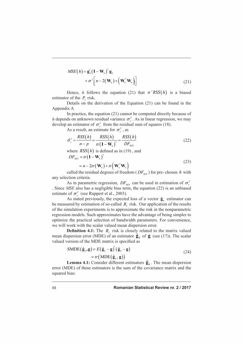
Romanian Statistical Review nr. 2 / 201788
2
2 2
h h h
h h h
MSE h
n
g I W g
W W W (21)
Hence, it follows the equation (21) that 1n RSS h is a biased estimator of the 2P risk. Details on the derivation of the Equation (21) can be found in the Appendix A In practice, the equation (21) cannot be computed directly because of it depends on unknown residual variance 2
. As in linear regression, we may develop an estimator of 2
from the residual sum of squares (18). As a result, an estimate for 2
, as
22ˆ
RESh
RSS h RSS h RSS hn p DFtr I W
(22)
where RSS h is defi ned as in (19) , and
2
2
RES h
h h h
DF tr
n tr tr
I W
W W W (23)
called the residual degrees of freedom ( RESDF ) for pre- chosen h with any selection criteria. As in parametric regression, RESDF can be used in estimation of 2
. Since MSE also has a negligible bias term, the equation (22) is an unbiased estimate of 2
(see Ruppert et al., 2003). As stated previously, the expected loss of a vector ˆ hg estimator can be measured by estimation of so-called 2R risk. Our application of the results of the simulation experiments is to approximate the risk in the nonparametric regression models. Such approximates have the advantage of being simpler to optimize the practical selection of bandwidth parameters. For convenience, we will work with the scalar valued mean dispersion error. Defi nition 4.1: The 2R risk is closely related to the matrix valued mean dispersion error (MDE) of an estimator ˆ hg of g (see (17)). The scalar valued version of the MDE matrix is specifi ed as
ˆ ˆ ˆSMDE
ˆMDE ,h h h
h
E
tr
g ,g g g g g
g g (24)
Lemma 4.1: Consider different estimators ˆ hg . The mean dispersion error (MDE) of these estimators is the sum of the covariance matrix and the squared bias:

Romanian Statistical Review nr. 2 / 2017 89
2
1
2
2 2
ˆ ˆSMDE ( ) ( )
ˆ
n
h i hii
h
h h h
E g X g X
E
tr
g
g g
I W g W W (25)
Proof: See Appendix B. As shown in the lemma 4.1 the SMDE matrix decomposes into a sum of the squared bias and variance of the estimator. Hence, we can compare the quality of two estimators by looking at the ratio of their SMDE in (25). This ratio gives the following defi nition concerning the superiority of any two estimators. Defi nition 4.2: The relative effi ciency of an estimator 1ˆ E hg compared to another estimator 2ˆ E hg is defi ned by the ratio,
1 1
2 2
ˆ ˆ, SMDEˆ ˆ, SMDE
E E
E E
R h hRE
R h h
g g g
g g g (26)
where .R denotes the scalar risk that is equivalent to the equation (24). 2ˆ E hg is said to be more effi cient than 1ˆ E hg if 1RE .
5. BANDWIDTH SELECTION CRITERIA
This section provides an overview of several criteria which have been used for smoothing parameter (or bandwidth) selection. The key idea is to select an appropriate value for the parameter h , bandwidth. As stated in previous section, the optimum h is defi ned as the smoothing parameter which minimizes the average of the mean square errors (AMSE), given by
22 2
ˆAMSE 1h hG
trn n
h I - W T W where hW is given in equation (16). The estimator of the error variance 2
is defi ned in the equation (22). The selection criteria are summarized as GCV Criterion: The criterion function is defi ned by Craven and Wahba (1979), and described as
2ˆ
21
1GCV( ) h G
h
-h
n n tr
I W T
I W
where hW , as is defi ned in (16), is smoother matrix based on h As in other criteria, to use GCV for parameter selection, we simply choose the parameter h giving smallest GCV over the set of parameter considered.

Romanian Statistical Review nr. 2 / 201790
AICc Criterion: Hurvich et. al., (1998) suggested an improved version of AIC which is called AICC, which is defi ned by
2ˆcAIC ( ) 1 log I
2 ( ) 1 ( ) 2
h G
h h
h n
tr n tr
W T
W W
BIC Criterion: The BIC is also called as Schwarz Information Criterion (SIC). The criterion is expressed as
2ˆBIC( ) 1
og( )h G
h
h n -
l n n tr
I W T
W
REML Criterion: The derivatives of both the REML and the GCV with respect to h can be determined quite naturally in a common form (see Reis et al., 2009). The REML score can be specifi ed as
2ˆREML( ) I ë hG
h - n tr W T W
CP Criterion: Mallows (1973) suggests the pC criterion in the regression case. If 2 is recognized, an unbiased estimate of the residual sum of squares is provided by pC criterion:
2 2 2ˆp
1( ) ( I) 2 ( )h hGC h tr
n W T W
Unless 2 is known, in practice an estimation for 2 can be given by (22). RECP Criterion: A direct computation leads to the bias-variance decomposition for ˆ( , ) hR g g :
2
2 2
1ˆ ˆ( ) = n
1 ( )
h h
h h h
R E
trn
g, g g - g
W I g W W
A clear–cut explanation shows that ˆ( , )= C ( )h pR hg g . Because the risk ˆ( , )hR g g is an unknown quantity, so-called risk is now estimated by computable quantity ˆ ˆ( , )
ph hR g g . The obtained expression for ˆ ˆ( , )ph hR g g is
p p
p p
2
22
1ˆ ˆ ˆ ˆ( ) = n
1 ˆ ˆ ( )
h h h h
h h h h h
R E
trn
g , g g - g
W I g W W
where p
2ˆh and p
ˆ hg are the appropriate pilot estimates for 2 and g, respectively. The pilot ph selected by classical methods. (see Lee, 2003-2004)

Romanian Statistical Review nr. 2 / 2017 91
6 SIMULATION EXPERIMENT
In this section we performed a Monte-Carlo simulation study to present and compare the kernel smoother estimators based on different bandwidth selection criteria given in section (4). To see the performance of the small, medium and large samples of each criterion we consider three censoring levels (CLs), 10%, 30%, and 50% and three samples sizes with n= 50, 100, and 200. The number of replication was 1000 for each of the samples. All calculations are carried out in MATLAB software. The empirical data is generated as;
( ) sin( 4.8 )sin(1.4 ) i i iT g X X X (27)
where 1
0.5
n
ii
iXn
and 2~ 0, 1i N .
6.1 Empirical Evaluations In our simulation study 54 different confi gurations are carried out. Furthermore, we used the MSE values to evaluate the quality of any curve estimate ( ˆˆ ( ) ( )h i h ig X g ):
n2
i ii =1
1 ˆ( ) ( )hMSE g X g Xn
(28) In the nonparametric regression setting, the outcomes from Monte Carlo simulation are illustrated in the following Tables and Figures. Table 1 compares the MSE values connected to the nonparametric regression models with right censored data under different censoring levels and sample sizes. The main idea is that a model with a better fi t denotes a minimum squared Euclidean distance between the data and fi tted values, and thus it has a minimum MSE value.

Romanian Statistical Review nr. 2 / 201792
MSE values from nonparametric regression models Table1
n = 50 CL=10% CL=30% CL=50%
AIC 0.067 0.129 0.201GCV 0.066 0.126 0.187RECP 0.063 0.111 0.170BIC 0.070 0.135 0.206
REML 0.067 0.131 0.204Cp 0.057 0.103 0.165
n = 100AIC 0.047 0.084 0.106GCV 0.047 0.084 0.105RECP 0.045 0.077 0.101BIC 0.054 0.095 0.117
REML 0.047 0.085 0.107Cp 0.037 0.065 0.090
n = 200AIC 0.035 0.059 0.069GCV 0.035 0.059 0.069RECP 0.037 0.059 0.075BIC 0.038 0.070 0.083
REML 0.036 0.059 0.069Cp 0.027 0.045 0.061
As expected, in Table 1, we obtained big MSE values for high censoring levels for all selection methods. Note also that although selection methods have good performances in general, BIC and REML methods gave bigger MSE values than AICc, GCV, RECP and Cp criteria. It means that their estimation performances are not good for bandwidth parameter under randomly right-censored data. The effect of the censoring, as expected, tends to increase the MSE values of the estimators, losing precision as the censoring level increases. In addition, and also as expected, the MSE values are improved as the sample size increases.

Romanian Statistical Review nr. 2 / 2017 93
Boxplots of the MSE values for estimated nonparametric modelsFigure 1
0
0.05
0.1
A1 G1 R1 B1 RM1 C1 A2 G2 R2 B2 RM2 C2 A3 G3 R3 B3 RM3 C3
0
0.1
0.2
A1 G1 R1 B1 RM1 C1 A2 G2 R2 B2 RM2 C2 A3 G3 R3 B3 RM3 C3
0
0.1
0.2
0.3
A1 G1 R1 B1 RM1 C1 A2 G2 R2 B2 RM2 C2 A3 G3 R3 B3 RM3 C3
Censorig Level=50%
Censorig Level=30%
Censorig Level=10%
Boxplots for MSE values based on each criterion are illustrated in Figure 1. In this Figure, A1, G1, B1, R1, RM1 and C1 denote the MSE values based on AICc, GCV, BIC, RECP, REML, and Cp selection criteria for sample sizes n=50, respectively. In a similar fashion, A2, G2, R2, B2, RM2 and C2 show the MSE values depend on the same criteria but for n=100. Finally, A3, G3, R3, B3, RM3 and C3 indicate the MSE values based on the mentioned criteria but for n=200. Also, the upper panel of Figure 1 has CL=10%, medium panel CL=30%, and bottom panel CL= 50%. As can be seen in Figure 1, as the sample size n gets large, the range of estimates are getting narrow. It can be said that the estimates from medium and large sized samples are more stable than those from small sized sample

Romanian Statistical Review nr. 2 / 201794
Real observations and the true function together with its smooth curves estimated by the selection criteria under different censoring levels
Figure 2
0 10 20 30 40 50-1
-0.5
0
0.5
1
1.5
2
X
0 10 20 30 40 50-1
-0.5
0
0.5
1
1.5
2
X
g(X
)
0 10 20 30 40 50-1
-0.5
0
0.5
1
1.5
2
X
g(X
)
0 10 20 30 40 50-1
-0.5
0
0.5
1
1.5
2
X
0 10 20 30 40 50-1
-0.5
0
0.5
1
1.5
2
X
g(X
)
0 10 20 30 40 50-1
-0.5
0
0.5
1
1.5
2
X
g(X
)
g(x)
g(%10)g(%30)
g(%50)
g(t)
g(10%)g(30%)
g(50%)
g(t)
g(10%)g(30%)
g(50%)
g(t)
g(10%)g(30%)
g(50%)
g(t)
g(10%)
g(30%)
g(50%)
g(t)
g(10%)g(30%)
g(50%)
GCV Method
REML Method RECP Method
BIC Method
Cp Method
AICc Method
As can be seen from Figures 2, the estimated functions move away from the real function when censoring levels increases, regardless of the sample sizes. Also, simulation experiment results show that the quality of estimated curves is reasonable for censoring levels, CL=10% and 30%, when compared to the CL=50%.
Real data points and the true function together with its smooth curves based on six selection criteria for n=50, and 10% and 50% censoring
levels, respectively.Figure 3
0 5 10 15 20 25 30 35 40 45 50-1
-0.5
0
0.5
1
1.5
X
g(X)
g(x)
g(AIC)
g(BIC)
g(GCV)
g(REML)
g(RECP)
g(Cp)
0 5 10 15 20 25 30 35 40 45 50-1
-0.5
0
0.5
1
X
g(X)
g(x)
g(AIC)
g(BIC)
g(GCV)
g(REML)
g(RECP)
g(Cp)
n=50, CL=50%
n=50, CL=10%

Romanian Statistical Review nr. 2 / 2017 95
As for Figure 3, we illustrate the true function together with their curves estimated by the selection criteria for samples sizes n = 50. In this Figure, the bottom panel represents the censoring level of 10%, while upper panel shows the same curves but for censoring level of 50%. As expected, the estimated smooth curves are closer to the real function when censoring levels decreases (see upper panel of the Figure 3). The estimated smooth curves in the Figure 4 exhibit a similar behaviour to Figure 3. That is, the curves obtained from the data with low censoring levels denote a better fi t from data with high censorship. Also, the effect of censoring levels makes much more impact on the estimated curves than sample sizes.
Similar to Figure 3, but for n=100 and 200.Figure 4
0 10 20 30 40 50 60 70 80 90 100-2
-1
0
1
2
X
g(X)
0 20 40 60 80 100 120 140 160 180 200-1
-0.5
0
0.5
1
X
g(X)
g(x)
g(AIC)
g(BIC)
g(GCV)
g(REML)
g(RECP)
g(Cp)
g(x)
g(AIC)
g(BIC)
g(GCV)
g(REML)
g(RECP)
g(Cp)
n=200, CL=50%
n=100, CL=10%
6.2 Comparing the effi ciency In this simulation study, to compare the effi ciency of the selection criteria based on different censoring levels and sample sizes we obtained the relative effi ciency matrix from the values of the SMDE ratios of the selection criteria. These values are computed using the equation (26) and they are given in Tables 2-3 for %10 and %50 censoring levels and all sample sizes. Outcomes correspond to %30 censoring levels are similar to the results displayed in Tables 2, they are not reported here. From Tables, we see that the relative effi ciency values of Cp method are smaller than 1 for all scenarios. Hence, it can be said that Cp is more effi cient than the other selection criteria for all sample sizes and censoring levels.

Romanian Statistical Review nr. 2 / 201796
Effi ciency values of selection criteria for 10% censoring level and all sample sizes
Table 2 AIC GCV RECP BIC REML Cp n = 50, CL=10%AIC 1.000 0.998 0.907 1.026 1.027 0.814GCV 1.001 1.000 0.909 1.028 1.029 0.815RECP 1.101 1.099 1.000 1.130 1.132 0.897BIC 0.974 0.972 0.884 1.000 1.001 0.793REML 0.973 0.971 0.883 0.998 1.000 0.792Cp 1.227 1.222 1.114 1.260 1.262 1.000 n=100, CL=10%AIC 1.000 1.000 0.930 1.118 1.026 0.772GCV 1.000 1.000 0.930 1.118 1.026 0.772RECP 1.075 1.075 1.000 1.202 1.103 0.830BIC 0.894 0.894 0.832 1.000 0.918 0.690REML 0.974 0.974 0.906 1.089 1.000 0.752Cp 1.295 1.295 1.204 1.447 1.329 1.000 n=200, CL=10%AIC 1.000 1.000 0.991 1.056 1.024 0.742GCV 1.000 1.000 0.991 1.056 1.024 0.742RECP 1.008 1.008 1.000 1.065 1.032 0.748BIC 0.946 0.946 0.938 1.000 0.969 0.702REML 0.976 0.976 0.968 1.031 1.000 0.724Cp 1.347 1.347 1.336 1.423 1.380 1.000
Findings of the simulation study may be summarized as follows: It is observed that the estimator using the Cp choice of bandwidth
parameter h dominates the other estimators for all scenarios. Inspection of the relative effi ciency values also reveal that for %50
censoring rate AIC criterion converges 1 highest at rates when sample size is large, n =200.
Notice that for all samples sizes and CL=%10, the AIC and GCV produce the same relative effi ciency values, whereas RECP gives the similar values to these criteria.
Simulated relative effi ciencies of BIC REML are not good and decreases dramatically with sample sizes, especially for %10 censoring levels.

Romanian Statistical Review nr. 2 / 2017 97
Effi ciency values of selection methods for %50 censoring level and all sample sizes
Table 3
AIC GCV RECP BIC REML Cp n = 50, CL=50%
AIC 1.000 0.953 0.848 1.024 1.017 0.822 GCV 1.048 1.000 0.889 1.074 1.066 0.862 RECP 1.179 1.124 1.000 1.207 1.199 0.969 BIC 0.976 0.931 0.828 1.000 0.993 0.803 REML 0.983 0.937 0.833 1.006 1.000 0.808 Cp 1.216 1.159 1.031 1.245 1.236 1.000
n=100, CL=50% AIC 1.000 0.998 0.932 1.105 1.014 0.830 GCV 1.001 1.000 0.934 1.107 1.016 0.832 RECP 1.071 1.070 1.000 1.184 1.087 0.890 BIC 0.905 0.903 0.844 1.000 0.918 0.751 REML 0.985 0.983 0.919 1.089 1.000 0.818 Cp 1.203 1.201 1.123 1.330 1.221 1.000
n=200, CL=50% AIC 1.000 1.000 1.055 1.184 1.006 0.853 GCV 0.999 1.000 1.055 1.184 1.006 0.853 RECP 0.947 0.947 1.000 1.122 0.953 0.808 BIC 0.844 0.844 0.890 1.000 0.849 0.720 REML 0.993 0.993 1.048 1.177 1.000 0.848 Cp 1.171 1.171 1.236 1.388 1.179 1.000
In the next section, we used a censored real data to see the process of the selection criteria.
7. REAL DATA EXAMPLE
To motivate the problem of the kernel type estimation procedure in nonparametric regression model with censored data, we used bowel cancer data obtained from cancer patients in Izmir city of Turkey. In here the logarithm of the survival times is considered as response (logT), while patient’s age is used as covariate (X). As seen from inspection of Figure 5, there is no strong evidence of a linear relationship between survival times and age. To see the relationship between survival time and age, the residuals are plotted against age in Figure 6. The nonlinearity is now more evident, especially because a scatterplot smooth has been added. This suggests that a nonparametric regression approach will be benefi cial..

Romanian Statistical Review nr. 2 / 201798
Scatterplot of age and lifetime dataFigure 5
10 20 30 40 50 60 70 80 90 100-1
0
1
2
3
4
5
Age
log(
Sur
viva
l Time)
The mentioned nonparametric regression model can be expressed as follows:
log ( ) , 1,..,218 i iisurvival times g age i
where survival times and age are defi ned as above, response and covariate, respectively. As previously mentioned, the key idea is to estimate the unknown function ( )g age . Various kernel estimates of these functions are obtained by using six selection criteria choice of bandwidth parameter, and showed in Figure 7.
Scatterplot residuals from regression of survival times on ageFigure 6

Romanian Statistical Review nr. 2 / 2017 99
As shown in Figure 7, there are six smooth functions that show the general trend of the data. These regression functions or smooth curves are also the plot of
1 218ˆ ˆ ˆ( ),..., ( ) gh h hg age g age
using (17), different nonparametric estimates of the effect of age variable on survival times . It is displayed six different smoothed curves for the kernel type estimators using the AICc, GCV, RECP, BIC, REML and Cp choice of bandwidth parameter h , respectively. The MSE values obtained from these kernel smoothing fi ts are 2.223, 2.225, 2.219, 2.233, 2.225 and 2.217, respectively. Thus, kernel fi ts of the nonparametric model obtained by AICc, GCV, RECP, BIC, and REML give similar performance, while Cp denotes a good performance in the estimation procedure.
Real observations and their smoothed curves obtained by six different kernel type estimators using six criteria choice of bandwidth parameter
Figure 7
10 20 30 40 50 60 70 80 90 100-1
0
1
2
3
4
5
Age
log(S
urviva
l Time)
Observationsg(AIC)g(GCV)g(RECP)g(BIC)g(REML)g(Cp)
8. CONCLUDING REMARKS
In this paper, we discussed the estimating the nonparametric regression function using kernel smoothing when the responses are subject to randomly right censoring data. Most important problem connected with the use of a kernel estimator is the selection of a good value of bandwidth parameter. In order to select this parameter, it is considered most widely used six different bandwidth selection criteria. Note also that we have focused on estimating the

Romanian Statistical Review nr. 2 / 2017100
bandwidth that minimizes the 2P risk or MSE. Thus we obtained six different kernel estimators by using bandwidth parameters that minimizes the selection criteria. This study is mainly conducted to evaluate the performances of the selection methods mentioned above. For these purposes, we used both simulated and real survival data examples. Consequently, as expected, we obtained big MSE values for high censoring levels for all selection methods. Also, as expected, the estimated smooth curves are closer to the real function when censoring levels decreases. As for selection criteria, it is observed that Cp has had the best empirical performance. However, BIC has produced the worst result. Finally, by considering the real data and simulation fi ndings given in the above, the following suggestions have to be taken into account: Cp criterion is recommended as being the best selection criteria for
all sample sizes and all censoring levels. For especially small sample sizes, the use RECP and GCV would be
more appropriate. For large samples, we propose the implementation of Cp or AICc
criteria.
Appendix A
We begin by considering the general defi nition of quadratic form, Theorem 1 and Lemmas 1-2 for proof of the equations (21) Defi nition A1: Let h ijw W = be a positive semi-defi nite and symmetrical n n matrix depend on the h and 1,...,
n be 1n a vector of random variables. Then
1 1q
n n
ij i j hi j
w
W (A1)
is a called a quadratic form in and hW is a called the matrix of a quadratic form. Theorem A1: If ijE Cov , and 0E , then
1 1
n n
h ij ij hi j
E w tr
W W
where (.)tr denotes trace of the matrix (.)

Romanian Statistical Review nr. 2 / 2017 101
Proof
1 1
1 1
1 1
( (
( ) ( )
( ) ( )
,
h
n n
ij i j i ji j
n n
ij i j i ji j
n n
ij i j hi j
E E E
E w E E
w E E E
w Cov tr
W
W
as claimed.
Theorem A2: Let be a 1n random vector with E and ijCov . Let Wh be a n n constant matrix. Then, the expected
value of the equation (A1)
h h hE tr W W W (A2) Proof It is well known that for i j ,
ij i j i jE and that for i j ,
2 2 2ij ii i i iE
According to (A1), the expected value of the quadratic form hW in expanded form as
1 1 1 1
E qn n n n
ij i j ij i ji j i j
E w E w
Since ij i j i jE , we obtain
i j ij i jE
Substituting,
1 1 1 1
1 1 1 1
E q
(A3)
n n n n
ij i j ij ij i ji j i j
n n n n
ij ij ij i ji j i j
w E w
w w
Note also that the terms ij are the elements of the variance-covarinace matrix . This matrix is a symmetric matrix whose ith element is the variance

Romanian Statistical Review nr. 2 / 2017102
of i and whose (ij)th off-diagonal element is the covariance between i and j .
It follows from (A1), and theorem 1 that the equation (A3) is equivalent to
h h hE tr W W W This completes the proof of the theorem 2. Again, let’s consider the equation (18)
ˆ ˆ
2
ˆ ˆ
ˆ ˆh hG G
hG G
RSS h
g T g T
= T I W T
Thus, from Theorems A1-A2 connected with quadratic form, the expected value of the RSS h is stated as
2
ˆ
2
ˆ
ˆ ˆ
2 22
2 2 2 2
2 2
ˆE
2
2
h G
G
G G
h h h h
h h h h h h
h h h h h h
RSS h MSE h E
E
E
tr
n
n
g T
I W T
T I W I W T
g I W g I W
g I W g W W W
g I W g W W W
as defi ned in the equation (21).
Appendix B
Proof of the Lemma 4.1
ˆSMDE hE g g , where ˆˆ h h Gg W T
Then the scalar valued version of the MDE matrix can be specifi ed as

Romanian Statistical Review nr. 2 / 2017 103
2
1
2
ˆ1
2
ˆ ˆ1
ˆ
2ˆ
2ˆ
ˆ ˆSMDE ( ) ( )
ˆ ( ) ( )
( )
n
h i hii
n
hi i h G ii
n
h i hG Gi ii
h G ii
h h G
h h hG
g X E g X
Cov g X g X E
Cov g X E
Cov
tr Cov
tr Cov
g
W T
W T W T
W T
I W g W T
I W g W T W
Assume that 2ˆ nG
Cov T I yields
2 2ˆSMDE h h h htr g I W g W W
REFERENCES: 1. Craven., P., and Wahba, G.,1979, Smoothing noisy data with spline functions., Num.
Math., 31,377-403. 2. Eubank, R. L., 1988, Spline Smoothing and Nonparametric Regression. Macal Dekker,
New York, 3. Hardle, W., Müller, M., 1997, Multivariate and Semiparametric Kernel Regression,
University of Humboldt Institute of statistics and Econometrics Berlin, Germany. 4. Hardle, W., 1990, Applied Nonparametric Regression, Cambridge University Press. 5. Hurvich, C., M., Simonoff, J. S., and Tasi, C. L, 1998, Smoothing parameter selection
in nonparametric regression using an improved Akaike information criterion., J.R. Statist. Soc. B., 60271-293
6. Koul, H., Susarla, V., Van Ryzin, J., 1981, Regression Analysis With Randomly Right-Censored Data, The Annals Of Statistics, 1276-1285.
7. Kaplan E. L., Meier, P., 1958, Nonparametric Estimation From İncomplete Observations, Journal Of The American Statistical Association, Vol. 53(282), 457-481.
8. Leurgans, S., 1987, Linear Models, Random Censoring and Synthetic Data, Biometrika Vol. 74, 301-309.
9. Mallows’, C., 1973, Some comments on Cp, Technometrics, 15,661-675. 10. Nadaraya, E. A., 1964, On estimating regression. Theory of Probability and its
Applications, pp.141–142. 11. Peterson, A. V. Jr., 1977, Expressing the Kaplan-Meier estimator as a function of
empirical subsurvival functions. J. Amer. Statist. Assoc. 72, 854-858. 12. Reis, P. T., & Ogden, R. T., 2009, Smoothing parameter selection for a class of
semiparametric linear models, J. R. Stat. Soc. B 71 (2009), pp. 505–523. 13. Ruppert D, Wand M, Carroll R, 2003, Semiparametric Regression. Cambridge
University Press, Cambridge, UK. 14. Schwarz, G., 1978, Estimating the dimension of a model, The Annals of Statistics, 6,
461-464. 15. Stute, W., Wang, J.-L., 1993, The Strong Law Under Random Censorship, Annals of
Statistics, 21,146-156.

Romanian Statistical Review nr. 2 / 2017104
16. Stute, W., 1993, Consistent Estimation Under Random Censorship When Covariables Are Present, Journal Of Multivariate Analysis,45,89-103.
17. Terrell, G.R., Scott, D.W., 1992, Variable kernel density estimation, Annals of Statistics, 20, 1236-1265.
18. Wang, Q.-H., Li, G., 2002, Empirical Likelihood Semiparametric Regression Analysis Under Random Censorship, Journal Of Multivariate Analysis, Vol. 83(2), 469-486.
19. Watson, G. S.,1964, Smooth regression analysis, Sankhya, Series A, vol.26, 359-72. 20. Wong, W. H., 1983, On the consistency of cross-validation in kernel nonparametric
regression, Annals of Statistics, Vol.11(4),1136-1141. 21. Van der Vaart, A. W., 1998, Asymptotic Statistics, Cambridge University press. 22. Vieu, P., 1991, Nonparametric regression: optimal local bandwidth choice, Journal of
he Royal Statistical Society Vol. 53(2), 453-464. 23. Zheng, Z. K., 1984, Regression Analysis wtih Censored Data, Ph.D Dissertation, Univ
of Colombia 24. Lee, Thomas C. M., 2004, Improved smoothing spline regression by combining
estimates of different smoothness, Statistics & Probability Letters, 67, 133-140. 25. Lee, Thomas C. M., 2003, Smoothing parameter selection for smoothing splines: a
simulation study, Computational Statistics & Data Analysis, 42, 139-148.