role of pectoral fin flexibility in robotic fish performance
TRANSCRIPT

J Nonlinear Sci (2017) 27:1155–1181DOI 10.1007/s00332-017-9373-6
Role of Pectoral Fin Flexibility in Robotic FishPerformance
Sanaz Bazaz Behbahani1 · Xiaobo Tan1
Received: 15 August 2016 / Accepted: 6 March 2017 / Published online: 11 March 2017© Springer Science+Business Media New York 2017
Abstract Pectoral fins play a vital role in the maneuvering and locomotion of fish,and they have become an important actuationmechanism for robotic fish. In this paper,we explore the effect of flexibility of robotic fish pectoral fins on the robot locomo-tion performance and mechanical efficiency. A dynamic model for the robotic fishis presented, where the flexible fin is modeled as multiple rigid elements connectedvia torsional springs and dampers. Blade element theory is used to capture the hydro-dynamic force on the fin. The model is validated with experimental results obtainedon a robotic fish prototype, equipped with 3D-printed fins of different flexibility. Themodel is then used to analyze the impacts of fin flexibility and power/recovery strokespeed ratio on the robot swimming speed and mechanical efficiency. It is found that, ingeneral, flexible fins demonstrate advantages over rigid fins in speed and efficiency atrelatively low fin-beat frequencies, while rigid fins outperform flexible fins at higherfrequencies. For a given fin flexibility, the optimal frequency for speed performancediffers from the optimal frequency for mechanical efficiency. In addition, for any givenfin, there is an optimal power/recovery stroke speed ratio, typically in the range of 2–3,that maximizes the speed performance. Overall, the presented model offers a promis-
Communicated by Maurizio Porfiri.
This work was supported by National Science Foundation (Grants IIP-1343413, IIS-1319602,CCF-1331852, ECCS-1446793).
B Xiaobo [email protected]
Sanaz Bazaz [email protected]
1 Smart Microsystems Laboratory, Department of Electrical and Computer Engineering, MichiganState University, East Lansing, MI 48824, USA
123

1156 J Nonlinear Sci (2017) 27:1155–1181
ing tool for fin flexibility and gait design, to achieve speed and efficiency objectivesfor robotic fish actuated with pectoral fins.
Keywords Robotic fish · Flexible pectoral fins · Dynamic model · Blade elementtheory · Mechanical efficiency
1 Introduction
Bio-inspired robotic fish aim to emulate swimming of live fish (Childress 1981; Blake1983) by deforming the body and/or moving different fins (Triantafyllou and Tri-antafyllou 1995;Mason and Burdick 2000a; Low 2006; y Alvarado andYoucef-Toumi2006; Ichiklzaki and Yamamoto 2007; Yu et al. 2012; Long et al. 2006). Improved effi-ciency,maneuverability, and stealth are some of the potential advantages of robotic fishover traditional propeller-driven underwater vehicles (Anderson et al. 1998; Sfakio-takis et al. 1999; Triantafyllou et al. 2000). Among their many applications, roboticfish can provide an underwater platform for aquatic environmental monitoring (Tan2011; Zhang et al. 2015), as well as serving as a tool for studying the behaviors of livefish through robot–animal interactions (Marras and Porfiri 2012). Numerous designsfor robotic fish have been reported in the literature (Du et al. 2015), with differentactuation mechanisms and levels of system complexity (Kopman and Porfiri 2013;Wang and Tan 2013; Behbahani et al. 2013; Kim et al. 2005; Wang et al. 2008; Aureliet al. 2010; Yu et al. 2004; Low andWilly 2006; Zhou et al. 2008; Ijspeert et al. 2007).
Modeling the robotic fish dynamics is often critical for the design, control, andunderstanding of robotic fish behavior, and it has received extensive attention in theliterature (Lighthill 1971;Morgansen et al. 2007; Aureli et al. 2010; Kanso et al. 2005;Wang and Tan 2013, 2015; Wang et al. 2015; Chen et al. 2010; Kelly and Murray2000; Kelly 1998). The most challenging step in dynamically modeling robotic fishis capturing the interactions between the body/fins and the fluid and calculating theresulting force andmoment exerted on the body. Computational fluid dynamics (CFD)modeling (Zhang et al. 2006; Liu et al. 1996; Mittal 2004; Dong et al. 2010) is capableof describing such interactions with high fidelity and offering physical insight, butits computational cost often makes it infeasible for designing and control purposes.Several alternatives are available. For example, quasi-steady lift and drag modelsfrom airfoil theory can be applied to the body and fin surfaces of underwater robots(Morgansen et al. 2007; Kodati et al. 2008; Harper et al. 1998; Mason and Burdick2000b; Mason 2003). One could also assume perfect fluids (irrotational potentialflow) and exploit the symmetry to obtain a finite-dimensional model for the fluid–structure interactions (Kanso et al. 2005; Melli et al. 2006). Effects of vorticity can beaccommodated by assuming, for example, vortices periodically shed from the tail fin(Kanso 2009; Kelly and Murray 2000).
In this work, we are focused on paired pectoral fin locomotion of a robotic fish.Although the caudal fin is the primary appendage used for propulsion in robotic fish(Lachat et al. 2006;Wang et al. 2008; Aureli et al. 2010;Wang and Tan 2013), pectoralfins play a vital role inmaneuvering and stability of livefishwhile providingor assistingpropulsion (Fontanella et al. 2013;Rosenberger 2001).Kinematics andhydrodynamics
123

J Nonlinear Sci (2017) 27:1155–1181 1157
of live fish pectoral fins have been studied be several researchers (Webb 1973, 1975;Blake 1979, 1980). A number of investigations have been conducted on rigid pectoralfinswith one ormore degrees of freedom, to study their effect on robotic fish swimming(Kato and Furushima 1996; Kato and Inaba 1998; Kato et al. 2000; Liu et al. 2005;Morgansen et al. 2007; Kodati et al. 2008; Sitorus et al. 2009). Recently, studies havebeen pursued on flexible pectoral fins (Kato et al. 2008; Lauder et al. 2006; Palmisanoet al. 2007; Tangorra et al. 2007; Barbera 2008; Phelan et al. 2010; Shoele and Zhu2010; Behbahani et al. 2013), and pectoral fins with flexible joints (Behbahani andTan 2014a, b, 2016a, b), to mimic live fish behavior more closely. While the flexibilityof pectoral fins for live fish and robotic fish is appreciated and has been explored withboth experimental (Lauder et al. 2006; Tangorra et al. 2007) and CFD (Dong et al.2010) methods, systematic analysis of the role of pectoral fin flexibility in robotic fishperformance has been limited.
The goal of this paper is to develop a systematic, computation-efficient frameworkfor analyzing how the flexibility of pectoral fins affects the swimming performanceand mechanical efficiency of the robot. While pectoral fin motions can generally beclassified into three modes based on the axis of rotation, rowing, feathering, andflapping, we focus on the rowing motion since it can be utilized for a number ofin-plane locomotion and maneuvering tasks, such as forward swimming, sidewayswimming, and turning. A dynamic model for the robotic fish is first proposed. Weuse Newton–Euler equations to model the rigid body dynamics of the robot. Theflexible fins are approximated as multiple rigid segments, connected via torsionalsprings and dampers. While the motion of the flexible fin in water could also bemodeled with the Euler–Bernoulli beam theory (Kopman et al. 2015; y Alvaradoand Youcef-Toumi 2006; Kopman and Porfiri 2013; Aureli et al. 2010; Wang et al.2015; Chen et al. 2010), the multi-segment approach has been proven effective andcomputationally efficient in capturing large deformation in flexible caudal fins (Wanget al. 2015). Blade element theory is adopted to evaluate the hydrodynamic forceson the fin elements. The proposed dynamic model is verified through experimentson a free-swimming robotic fish prototype equipped with pectoral fins. The fins are3D-printed with different stiffness levels, ranging from very flexible to rigid.
The dynamic model is used to analyze the impact of fin flexibility on swimmingspeed behavior at different fin-beat frequencies. It is found that, while the robot withrigid fins achieves a linearly increasing speed with the fin-beat frequency, there isan optimal frequency in the case of a flexible fin at which the speed is maximized.Furthermore, fins with moderate flexibility outperform the rigid fins on the speedperformance for a large range of operating frequencies. The impact of speed ratioζ between the power stroke and the recovery stroke on the swimming behavior isalso studied for different fins. Finally, the influences of fin flexibility and ζ on themechanical efficiency of the robot are examined. The study reveals interesting trade-offs between the different objectives (speed and efficiency) and supports the use ofthe proposed model as a promising tool for fin flexibility and gait design.
The remainder of this paper is organized as follows. Section 2 reviews the dynamicsof the robotic fish body. Section 3 presents the dynamic model for the flexible pectoralfins. The kinematics of the flexible pectoral fins adopted in this work is presented inSect. 4, while the method for mechanical efficiency calculation is discussed in Sect. 5.
123

1158 J Nonlinear Sci (2017) 27:1155–1181
In Sect. 6, we present the robotic fish prototype, the pectoral fin fabrication method,the experimental setup, and the methods for model parameter identification. Section7 is devoted to results. Finally, concluding remarks and future work directions arediscussed in Sect. 8.
2 Dynamics of the Robotic Fish Body
The robotic fish under study contains two subsystems, the flexible pectoral fins, forwhich the dynamics are covered in Sect. 3, and the rigid body. The robotic fish proto-type used in this study does have a caudal fin, but the consideration of hydrodynamicsassociated with an actuated caudal fin is outside the scope of this work. Instead, the(unactuated) caudal fin is considered part of the rigid body. To study the motion of therobot, we include the rigid body dynamics based on Kirchhoff’s equations of motionin an inviscid fluid (Fossen 1994; Aureli et al. 2010), with the added mass effectincorporated.
2.1 Rigid Body Dynamics
Figure 1 illustrates a robotic fish, restricted to the planar motion, where [X,Y, Z ]Tdenotes the global coordinates, and [x, y, z]T with unit vectors [i, j, k] indicates thebody-fixed coordinates, attached to the center of mass of the robotic fish body. Eachpectoral fin is modeled as multiple, connected, rigid elements, and mi and ni denotethe unit vectors parallel to and perpendicular to the i th element of the pectoral fin,respectively, where superscripts r and l indicate the right and the left fin, respectively.
Y
XZ
A0
xy
z
VC
FD
FL
ij
k
1l
MD
Cz
l2
2r
1r
ˆ lin
ˆ lim
ˆ rin
ˆ rim
li
ri
Fig. 1 Top view of the robotic fish actuated by flexible pectoral fins and restricted to planar motion
123

J Nonlinear Sci (2017) 27:1155–1181 1159
The robotic fish body and the flexible pectoral fins are considered to be neutrallybuoyant, with center of gravity and geometry coinciding. The simplified equations ofthe robotic fish body in the body-fixed coordinates are represented as (Barbera 2008;Wang et al. 2015; Behbahani and Tan 2016b)
(mb − XVCx)VCx = (mb − YVCy
)VCyωCz + Fx , (1)
(mb − YVCY)VCy = −(mb − XVCx
)VCxωCz + Fy, (2)
(Iz − NωCx)ωCz = Mz, (3)
where mb is the mass of the robotic fish body, Iz is the robot inertia about the z-axis,and XVCx
,YVCy, and NωCx
are the hydrodynamic derivatives that represent the effect
of the added mass/inertia on the rigid body (Fossen 1994). VCx , VCy , and ωCz are thesurge, sway, and yaw velocities, respectively. The variables Fx , Fy and Mz denotethe external hydrodynamic forces and moment exerted on the fish body, which aredescribed as
Fx = Fhx − FD cosβ + FL sin β, (4)
Fy = Fhy − FD sin β − FL cosβ, (5)
Mz = Mhz + MD, (6)
where Fhx , Fhy , and Mhz are the hydrodynamic forces and moment transmitted to thefish body by the pectoral fins, the details of which are provided in Sect. 3. As depictedin Fig. 1, FD, FL, and MD are the body drag, lift, and moment, respectively. Theseforces and moment are expressed as (Morgansen et al. 2007; Aureli et al. 2010; Wanget al. 2015)
FD = 1
2ρ|VC |2SACD, (7)
FL = 1
2ρ|VC |2SACLβ, (8)
MD = −CMω2Cz
sgn(ωCz ), (9)
where |VC | is the linear velocity magnitude of the robotic fish body, |VC | =√V 2Cx
+ V 2Cy
, ρ is the mass density of water, SA is the wetted area of the body,CD,CL
and CM are the dimensionless drag, lift, and damping moment coefficients, respec-tively, β is the angle of attack of the body, and sgn(.) is the signum function.
Finally, the kinematics of the robotic fish are described as (Wang et al. 2015)
X = VCx cosψ − VCy sinψ, (10)
Y = VCy cosψ + VCx sin ψ, (11)
ψ = ωCz , (12)
where ψ denotes the angle between the x-axis and the X -axis.
123

1160 J Nonlinear Sci (2017) 27:1155–1181
3 Dynamics of Flexible Rowing Pectoral Fins
This section focuses on calculating the hydrodynamic forces on the flexible pectoralfin and determining its dynamics using blade element theory (Blake 1983), by dividingthe fin span into multiple rigid elements. The rowing motion of the pectoral fin hasbeen classified as a “drag-based” swimming mechanism, where the drag element offluid dynamics generates the thrust (Lauder and Drucker 2004; Vogel 1994). Thepectoral fin is considered to be rectangular with span length of S and chord length ofC . We consider a coordinate system with unit vectors mi and ni for the pectoral fin;see Fig. 1. The relationship between these unit vectors and the robotic fish body-fixedcoordinates is given by
mi = cos γi i + sin γi j, (13)
ni = − sin γi i + cos γi j, (14)
where γi is the angle between mi and i ; see Fig. 1 for illustration. We use the leftpectoral fin to illustrate the calculations. However, it is straightforward to extend thecalculations to the right pectoral fin. Figure 2 provides a visualization of the parametersand variables of a flexible fin element.
We divide the flexible fin into N rigid elements with an equal length of l = SN ,
where each segment is connected to its neighbors via a pair of torsional spring anddamper. The constants of the spring and damper can be derived from the properties ofthe flexible material. The spring constant KS is evaluated as (Banerjee and Nagarajan1997)
KS = ECh3
12l, (15)
where h is the beam thickness and E is the Young’s modulus of the flexible materialused for the pectoral fin. The damper coefficient KD can be evaluated as KD = κKS,where κ is a proportional constant. Figure 3 illustrates the forces on the i th element of
Top viewView from the directionn
i
j
dih
Fi
iv
ˆin
ˆ im
i
ds
C
sˆin
ˆ im
1iA
SN
Fig. 2 Top view of i th element of the flexible fin and its parameters and variables
123

J Nonlinear Sci (2017) 27:1155–1181 1161
i
Torsion spring and damper
th elementi
(i+1)
j
,iA yF
( 1) ,iA xF
( 1) ,iA yF
,iA xF
,ih xF,ih yF
0A1A
1iA
iA
i
Fig. 3 Illustration of forces on the i th element of the flexible fin
the flexible fin. The angle γ1 is dictated by the pectoral fin actuator, and we need to findthe angles γ2 to γN , to know the trajectory of the flexible fin at each instant of time,which, subsequently, will allow one to evaluate the hydrodynamic force generated bythe fin. In the following calculations, we assume an anchored robotic fish body. Whileconsidering the body motion in computing the hydrodynamic force on the actuatedfin is instrumental in capturing the coupling between propulsion and robot motion(Kopman et al. 2015; Wang and Tan 2013), it significantly increases the modelingand subsequent computational complexity. In this work, the pectoral fin tip velocity istypically about ten times of the robotic fish body velocity; therefore, themodeling errorintroduced by ignoring the body motion is acceptable. This simplifying assumptionhas been adopted in the literature for robotic fish propelled with a caudal fin (Kopmanand Porfiri 2013; Wang et al. 2015; y Alvarado and Youcef-Toumi 2006), and in ourearlier work on rigid pectoral fins with flexible joints (Behbahani and Tan 2016a, b),where a similar robotic fish prototype was used.
The position of each point s on the i th element (see the definition of s in Fig. 2) attime t on the i th element can be described as
ri (s, t) =i−1∑k=1
l · mk + s · mi . (16)
The corresponding velocity at the point s is
vi (s, t) ={
i−1∑k=1
lγk cos(γi − γk) + sγi
}ni +
{i−1∑k=1
lγk sin(γi − γk)
}mi , (17)
123

1162 J Nonlinear Sci (2017) 27:1155–1181
where γk indicates the time derivative of γk . Respectively, the corresponding acceler-ation at the point s is evaluated as
ai (s, t) ={
i−1∑k=1
[lγk cos(γi − γk) + lγ 2
k sin(γi − γk)]
+ sγi
}ni
+{
i−1∑k=1
[lγk sin(γi − γk) − lγ 2
k cos(γi − γk)]
− sγ 2i
}mi ,
(18)
where γk indicates the second time derivative of γk .
3.1 Force Calculations for Element i
The hydrodynamic force on each element of the flexible fin is evaluated based on theblade element theory (Blake 1983) as follows
dFhi (s, t) = −1
2Cn
(αi (s, t)
)ρC |vi (s, t)|2ds evi , (19)
where evi is a unit vector in the direction of the velocity of the i th element. Cn is theforce coefficient, which depends on the angle of attack at each point, αi (s, t), and hasa form of
Cn(αi ) = λ sin αi , (20)
where the parameterλ is evaluated empirically through experiments. Note that Eq. (19)captures both normal and span-wise components of the hydrodynamic force. The angleof attack at each point, αi (s, t), is defined via
tan αi (s, t) = 〈vi (s, t), ni 〉〈vi (s, t), mi 〉 , (21)
where 〈·, ·〉 denotes the inner product.The total hydrodynamic force acting on the i th element is defined by integrating
Eq. (19) along the length of the element
Fhi (t) =∫ l
0dFhi (s, t). (22)
The interaction between two consecutive elements is captured via force balance oneach element:
Fhi + FAi−1 − FAi = miai , (23)
123
J Nonlinear Sci (2017) 27:1155–1181 1163
where FAi is the force applied by element i on element i + 1, FAi−1 is the forceapplied by element i − 1 on element i,mi is the effective mass of the i th element(which contains the mass and the added mass of element i , where the added mass iscalculated based on a rigid plate moving in the water), and ai denotes the accelerationof the midpoint of the i th element, which can be evaluated using Eq. (18) with s = l
2 .See Fig. 3 for illustration of the forces. Note that for the last element, FAN = 0;therefore, Eq. (23) can be solved iteratively for FAi , where 0 ≤ i ≤ N − 1.
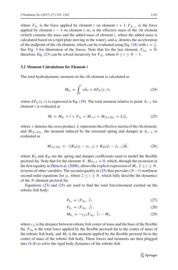
3.2 Moment Calculations for Element i
The total hydrodynamic moment on the i th element is calculated as
Mhi =∫ l
0smi × dFhi (s, t), (24)
where dFhi (s, t) is expressed in Eq. (19). The total moment relative to point Ai−1 forelement i is evaluated as
Mi = Mhi + l × FAi + Mi+1 + M(S+D)i = Ii γi , (25)
where× denotes the cross product, Ii represents the effective inertia of the i th element,and M(S+D)i , the moment induced by the torsional spring and damper at Ai−1, isevaluated as
M(S+D)i = −[KS(γi − γi−1) + KD(γi − γi−1)]k, (26)
where KS and KD are the spring and damper coefficients used to model the flexiblepectoral fin. Note that for the element N , MN+1 = 0, which, through the recursion inthe first equality in Zhou et al. (2008), allows the explicit expression ofMi , 2 ≤ i ≤ N ,in terms of other variables. The second equality in (25) thus provides (N−1) nonlinearsecond-order equations for γi , where 2 ≤ i ≤ N , which fully describe the dynamicsof the N -element pectoral fin.
Equations (23) and (25) are used to find the total force/moment exerted on therobotic fish body:
Fhx = 〈FA0 , i〉, (27)
Fhy = 〈FA0 , j〉, (28)
Mhz = −cp〈FA0 , i〉 − M1, (29)
where cp is the distance between robotic fish center of mass and the base of the flexiblefin, FA0 is the total force applied by the flexible pectoral fin to the center of mass ofthe robotic fish body, and M1 is the moment applied by the flexible pectoral fin to thecenter of mass of the robotic fish body. These forces and moments are then pluggedinto (4–6) to solve the rigid body dynamics of the robotic fish.
123

1164 J Nonlinear Sci (2017) 27:1155–1181
4 Kinematics of Flexible Rowing Pectoral Fins
The pectoral fins in this study sweep back and forth within the frontal plane. Therowing motion has distinct power and recovery strokes. During the power stroke, thepectoral finmoves backward to produce thrust through induced drag on the pectoral finsurface. On the other hand, during the recovery stroke, the fin moves toward the frontof the fish, with minimal loading, to get ready for next fin-beat cycle. The pectoralfin is actuated at different speeds during the power and recovery strokes (faster powerstroke) to produce a net thrust. In particular, we define the ratio
ζ = P
R= Power stroke speed
Recovery stroke speed. (30)
For each fin-beat cycle, the pectoral fin base rotates according to
γ1(t) =⎧⎨⎩
π2 − γA cos
[π
(ζ+1Tp
)t], 0 ≤ t ≤ Tp
ζ+1
π2 + γA cos
[π
(ζ+1ζTp
)(t − Tp
ζ+1
)],
Tpζ+1 < t ≤ Tp
(31)
where γA is the amplitude of fin the actuation and TP denotes the period of one cycle.Figure 4 illustrates the pectoral fin kinematics. The visualization of the pectoral
fin motion during one fin-beat cycle is shown in Fig. 4a. Note that for ζ = 1, the
RP
0t2( 1)
pTt1
pTt2
2( 1) pt T pt T
(a)
060
70
80
90
100
110
120
Ang
le (D
egre
e)
Time (s)
Tp/2( ) Tp/( ) [(2+ )/2( )]Tp Tp-20
0
20
40
60
80
0
Time (s)
Tp/2( ) Tp/( ) [(2+ )/2( )]Tp Tp
Ang
le v
eloc
ity (D
egre
e/s)Power stroke Recovery stroke Power stroke Recovery stroke
(b)
Fig. 4 Illustration of the pectoral fin motion during power and recovery strokes: a the snapshots at differenttime instances of one fin-beat cycle, where Tp represents the total time for each cycle; b orientation andangular velocity of the base of the pectoral fin with respect to the main axis of the robotic fish, whereζ = 5, γrmA = 50 deg, and Tp = 1 s are used
123

J Nonlinear Sci (2017) 27:1155–1181 1165
pectoral fin flaps symmetrically during the power stroke and the recovery stroke, andfor ζ > 1, the pectoral fin slows down and spends more time in the recovery phase.Figure 4b illustrates the orientation angle γ1 and the angular velocity γ1 of the base ofthe pectoral fin with respect to the x-axis of the robotic fish during one fin-beat cycle.For turning the robotic fish, we just actuate one of the pectoral fins and keep the otherfin still.
5 Mechanical Efficiency
Aside from the swimming performance (for example, swimming speed or turningradius), another critical factor about the robotic fish is its mechanical efficiency. Wewill analyze the efficiency of the robot under different pectoral fin properties usingthe model presented in Sects. 3 and 4. In particular, it is of interest to investigate theeffect of flexibility of the pectoral fins on the mechanical efficiency. During steady-state swimming, the mechanical efficiency of the robot is evaluated as (Blake 1983;Nakashima et al. 2003; Suzuki et al. 2007)
η = Wb
WT, (32)
whereWb is the useful work needed to move the robotic fish during each fin-beat cycleandWT is the total work done by the pectoral fins during the same period. In this study,we do not consider other energy losses, such as the amount of electrical power usedby other electronics, or frictional losses in motors and gears. The useful work Wb isdetermined by
Wb =∫ t0+Tp
t0FThrust(t)VCx (t)dt, (33)
where t0 denotes the beginning of the fin-beat cycle and FThrust = Fhx is the totalhydrodynamic force produced by the pectoral fin in the x direction, exerted on therobotic fish body. The total work done by the paired pectoral fins,WT, is obtained via
WT = 2∫ t0+Tp
t0max
{0,
N∑i=1
∫ l
0〈dFhi (s, t), vi (s, t)〉
}dt. (34)
At some instants of time, the mechanical power of the pectoral fins could be negative.However, the servos cannot reclaim this energy from the water. Therefore, we treat theinstantaneous power for these cases to be zero, which explains the max(0, ·) operationin (34).
123

1166 J Nonlinear Sci (2017) 27:1155–1181
6 Materials and Methods
6.1 Robotic Fish Prototype
A robotic fish prototype, similar to that in Behbahani and Tan (2016a), was used to testandvalidate the proposeddynamicmodel and to support the performance analysis. Thisrobotic fish included a rigid body, two pectoral fins, and a caudal fin. The rigid bodywas designed in SoildWorks software and printed in the VeroWhitePlus material froma PolyJet multi-material 3D printer (Objet350 Connex 3D System from Stratasys)and was coated with acrylic paint to minimize water absorption of the 3D-printedmaterial. The body had a length of 15 cm, height of 8 cm, and width of 4.6 cm. Threewaterproof servomotors (Traxxas 2065 Waterproof Sub-Micro Servo from Traxxas)was used to move the pectoral fins and caudal fin individually. The robot was battery-operated, using a Li-ion rechargeable battery (7.4 V, 1400mAh from Powerizer), and acustomized power converter PCBwas designed to regulate the voltage to 5 V (throughLM2673) and 3.3 V (through LP38690) for the servomotors and the microcontroller,respectively. The robot fin motion was controlled by a microcontroller (Arduino ProMini, 3.3 V). A picture of the 3D-printed body, along with all the other componentsfor the robot, is shown in Fig. 5.
6.2 Pectoral Fin Fabrication
The pectoral fins used in this study were designed to have a composite structure andwere 3D-printed. The fins could be easily detached from the fin mounts, to enabletesting of the robot with different fins. We followed the approach proposed in Clarket al. (2015) for creating the composite fins, the effective stiffness of which can beeasily adjusted by changing the thicknesses of different layers. The composite finswere made of two different materials, a rigid plastic material (VeroWhitePlus) and aflexible rubberlike material (TangoBlackPlus). The details of the design are illustratedin Fig. 6. The flexibility of the fins was controlled by adjusting the thickness ofthe VeroWhitePlus inner layer while keeping the total thickness of the fin constant(1.2 mm). Pectoral fins of size 45 mm × 37.5 mm, with three different stiffness
3D printed body
On/Off Switch
Charging port
WP Servos
Power board
Microcontroller & Programming port
Rechargeable battery
Flexible Fin
Motion detection markers
Fig. 5 3D-printed robotic fish body and other components of the robot
123

J Nonlinear Sci (2017) 27:1155–1181 1167
tinner
1.2 mm
VeroWhitePlus
TangoBlackPlus
Fig. 6 Solidworks design of a composite pectoral fin
Table 1 Specifications ofpectoral fins with differentflexibilities
Fin name tinner (mm) KS (Nm) KD (Nms)
F1 1.2 NA NA
F2 0.3 1.13 × 10⁻³ 2.59 × 10⁻⁴
F3 0 1.83 × 10⁻⁴ 4.37 × 10⁻⁵
Fig. 7 An actual 3D-printed pectoral fin. Right Original fin; left printed fin treated with Ultra-Ever Dryomniphobic material
values, were fabricated. The specifications of these fins are summarized in Table 1.The fins are named F1–F3 for later reference in this paper.
The 3D-printed pectoral fins were treated with a thin coat of Ultra-Ever Dry omni-phobic material (UltraTech International Inc.) to prevent changes of properties thatmay occur when they come in contact with water. Figure 7 shows an actual 3D-printedpectoral fin, before and after the Ultra-Ever Dry treatment. The application of Ultra-Ever Dry results in a white cast on the treated part.
6.3 Experimental Setup
Experimentswere conducted in a 6-ft-long, 2-ft-wide, and 2-ft-deep tank.AnOptitrackmotion capture system, containing four Flex 13 cameras, each mounted on heavy-duty
123

1168 J Nonlinear Sci (2017) 27:1155–1181
Camera #1
Camera #2, #3
Camera #4
Robotic Fish
(a)
Robotic Fish
Cameras
(b)
Fig. 8 Experimental setup: a actual, b output of the Motive software
universal stand via Manfrotto super clamp and 3D junior camera head, was used totrack the robotic fish swimming. A computer equipped with Motive 1.7.5 software,capable of supporting real-time and offline workflows, was used to extract the desireddata. The details of this setup are shown in Fig. 8. Two different locomotion modes,forward swimming and turning, were adopted for the robotic fish in the experiments.For each experiment, the robotic fish swam for approximately 30 s to reach its steady-statemotion, and then, the steady-state datawere captured and extracted. In the forwardswimming case, we recorded the time it took for the robot to swim a distance of 50 cm.The experiment for each setting was repeated ten times, to minimize the impact ofrandom factors on the experimental results.
6.4 Parameter Identification
All the parameters used in the simulations were either measured directly or identifiedexperimentally. Details of the identification procedure for parameters of the roboticfish body can be found in Behbahani and Tan (2016a, b). The mass of the robotic fishwas mb = 0.502 kg, and the inertia was evaluated to be Iz = 7.26 × 10⁻⁴ kg/m2.The added masses and added inertia were calculated based on a prolate spheroidapproximation for the robotic fish body (Aureli et al. 2010; Fossen 1994), which were−XVCx
= 0.1619 kg, −YVCy= 0.3057 kg, and −NωCx
= 5.52 × 10⁻⁵ kg/m2. The
wetted surface area of the robotic fish body was SA = 0.0325m2. The drag, lift,and moment coefficients were identified empirically, using the rigid pectoral fins andζ = 2. In particular, these parameterswere tuned tomatch the forward velocity, turningradius, and turning period obtained in simulation with the experimental measurement,when two different power stroke speeds are used, completing the power stroke in0.5 and 0.3 s, respectively. The resulting coefficients were CD = 0.42,CL = 4.86,and CM = 7.6 × 10⁻⁴ kg/m2. The parameter λ from Eq. (20), which represents thehydrodynamic force coefficient of the pectoral fin, was identified empirically to be 0.6,by matching the forward swimming velocity of the robotic fish utilizing rigid pectoralfins for the fin-beat frequencies of 1 and 1.667 Hz, and power/recovery stroke ratio
123

J Nonlinear Sci (2017) 27:1155–1181 1169
ζ = 2. This parameter was then used for all the other fin-beat frequencies, pectoralfin flexibilities, and ζ ratios.
The spring and damper coefficients of the flexible fins were tuned to match theforward swimming velocity and the turning period of the robotic fish collected fromexperiments for ζ = 2, and fin-beat frequencies of 1 and 1.667 Hz. Each fin is dis-cretized into three elements. The parameters for each fin are summarized in Table 1.These numbers were then used for all the other fin-beat frequencies and ζ ratiosthroughout the simulations. We note that the choice of the number of approximatingrigid segments is an important issue. Clearly, the more elements, the more accu-rate approximation to the flexible fin shape, at the cost of increased computationalcomplexity. It is also reasonable to use more rigid elements for more flexible fins.However, the equations for the fin dynamics (γi equations) are highly nonlinear; forexample, Eqs. (17) and (19) imply that the hydrodynamic force depends on terms likeγ 2k sin2(γi − γk)). The latter makes solving these equations in their current form very
challenging when the number of elements gets big. As a result, we have found thatthree segments provide an acceptable trade-off between the modeling accuracy andcomputational cost, and the good match between the experimental results and modelpredictions reported in Sect. 7 also suggests that the three-segment approximation isreasonable.
7 Results and Analysis
7.1 Dynamic Model Validation
First, we have included plots of simulation results to illustrate how the flexible pectoralfin moves. The time history of the angles of different elements of the flexible pectoralfin, and the respective angles of attack, is shown in Fig. 9. In this simulation, theflexible fin F2 was used. Note the clear phase lags between the consecutive elements’angles γi . The angles of attack for all elements are constant (90◦ or −90◦) for mostof the time, but they experience abrupt changes during the transition between powerand recovery strokes.
Next, we present results that validate our proposed dynamic model, where the caseof pectoral fin F2 with ζ = 2 is used. Additional results supporting the model canbe found in Sect. 7.2. Figure 10 shows the comparison between model predictionsand experimental measurements of the forward swimming velocity, reported in bothcm/s and body length per second (BL/s) versus the fin-beat frequency. The fin-beatfrequency is defined as 1
Tp, where Tp is the duration of each fin-beat cycle. In the
experiments, for ζ = 2, the speed limit of the servo motors translated to a maximumactuation frequency of 2 Hz, so we have extended the simulation results to fin-beatfrequency of 3 Hz in order to capture the performance trend of the robotic fish. FromFig. 10, the speed of the robotic fish drops after the fin-beat frequency reaches anoptimal value, beyond which it gets harder for the flexible pectoral fins to follow theprescribed servo motion, and thus, the fin oscillation amplitude drops, resulting in adropping thrust and speed as the frequency gets higher. Figures 11 and 12 show acomparison between simulation and experimental results on the turning period and
123

1170 J Nonlinear Sci (2017) 27:1155–1181
0 0.5 1 1.5 2 2.5 360
70
80
90
100
110
120A
ngle
(Deg
ree)
Time (s)
Element 1Element 2Element 3
(a)
-150
-100
-50
0
50
100
150
0 0.5 1 1.5 2 2.5 3
Time (s)
Ang
le o
f atta
ck (D
egre
e)
Element 1Element 2Element 3
(b)
Ang
le o
f atta
ck (D
egre
e)
Time (s)
0 0.1 0.2 0.3 0.4 0.589
97.5
106
1 1.5 2 2.5 3-91.5
-90.25
-89
Element 1Element 2Element 3
Element 1Element 2Element 3
Power Stroke
Recovery Stroke
(c)
Fig. 9 Time history of flexible pectoral fin: a evolution of the rigid element angles γ1–γ3, for onemovementcycle, b variation of the angles of attack for all elements, where ζ = 5, γA = 50 deg, and Tp = 3 s, czoom-in view of the angle of attack for one movement cycle
Forw
ard
velo
city
(BL/
s)
0.5 1 1.5 2 2.5 30.5
11.5
22.5
33.5
44.5
Fin-beat frequency (Hz)
Forw
ard
velo
city
(cm
/s)
0.033
0.0670.10.1330.167
0.20.230.2670.3
ExperimentSimulation
Fig. 10 Case of F2 with ζ = 2: comparison between dynamic model simulation and experimental mea-surement of the forward swimming velocity, for different fin-beat frequencies
the turning radius versus fin-beat frequency, respectively. In Fig. 11, the turning perioddrops with the fin-beat rate, as expected, up to a particular optimal frequency, beyondwhich it starts to increase. The optimal frequency in Fig. 11 coincides with that inFig. 10. This can be explained by that, in both cases, the hydrodynamic forces generatedby each pectoral fin are correlated with the fin oscillation amplitude, the behavior ofwhich follows the same frequency response given our anchored-body assumption. Thesimulation results in Fig. 12 suggest that the turning radius of the robotic fish is nearlyindependent of fin-beat frequencies. The experimental data support the simulation tosome extent. The mean of the turning radius remains almost the same (between 16 and
123

J Nonlinear Sci (2017) 27:1155–1181 1171
0.5 1 1.5 2 2.5 30
20
40
60
80
100
Fin-beat frequency (Hz)
Turn
ing
perio
d (s
) ExperimentSimulation
Fig. 11 Case of F2 with ζ = 2: comparison between dynamic model simulation and experimental mea-surement of the turning period, for different fin-beat frequencies
0.5 1 1.5 2 2.5 310
15
20
25
Fin-beat frequency (Hz)
Turn
ing
Radi
us (c
m)
Turn
ing
Radi
us (B
L)
0.6667
1.0000
1.3333
1.6667
ExperimentSimulation
Fig. 12 Case of F2 with ζ = 2: comparison between dynamic model simulation and experimental mea-surement of the turning radius, for different fin-beat frequencies
18 cm) for different fin-beat frequencies. Due to the disturbances from the interactionbetween the fluid and the tank wall, the robotic fish typically would not stay repeatedlyon the same orbit in each turning experiment, which inevitably introduced noticeableerror in the turning radius measurement.
Overall, it can be concluded from Figs. 10, 11, and 12 that the proposed dynamicmodel can well capture the motion of the robotic fish actuated by flexible pectoralfins. Additional results in Sect. 7.2 will further validate the model through good matchbetween experimental and simulation results.
7.2 Impact of Fin Stiffness
Here we compare the performance of pectoral fins with different flexibilities to gaininsight into the influence of fin flexibility. We utilized a fin-beat pattern as specifiedin (31), where ζ = 2. The simulation and experimental results, shown in Fig. 13,are reported in both cm/s and BL/s. Again, we have extended the simulation results tofin-beat frequency of 3 Hz in order to capture the performance trend of the robotic fish.From Fig. 13, it is interesting to note that with rigid fins (F1), the swimming velocity
123

1172 J Nonlinear Sci (2017) 27:1155–1181
0.5 1 1.5 2 2.5 30.5
11.5
22.5
33.5
44.5
5
Fin-beat frequency (Hz)
Forw
ard
velo
city
(cm
/s) Exp – F1 Sim – F1
Exp – F2 Sim – F2Exp – F3 Sim – F3
Forw
ard
velo
city
(BL/
s)
0.0330.0670.10.1330.1670.20.230.2670.30.333
Fig. 13 Experimental and simulation results on the forward swimming velocity versus fin-beat frequencyfor different flexibilities of the pectoral fin, where the power/recovery stroke ratio ζ = 2 for all cases
increases nearly linearly with the fin-beat frequency, while for the flexible fins (F2 andF3), there is a clear optimal frequency at which the velocity is maximum. Fins withmoderate flexibility (F2) outperform the rigid fins (F1) for the entire fin-beat frequencyrange achievable by the robotic fish prototype. This can be explained by that the flexiblefin F2 moves beyond the line defined by the servo shaft, while the rigid fin alwaysmoves in sync with the servo shaft line, resulting in a larger oscillation amplitudefor the flexible fin (until the frequency is high enough). The optimal frequency ofoperation for the flexible fin case is believed to be correlated to the resonant frequencyof the fin in water, which drops as the flexibility of the fin increases. When the fin istoo flexible (F3), its movement is greatly constrained by the resistance from water,which explains the corresponding poor swimming performance for the robotic fish.
7.3 Impact of the Power to Recovery Stroke Speed Ratio
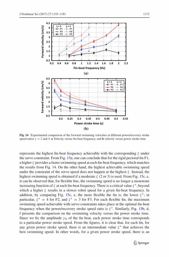
This subsection is devoted to studying the effect of the power to recovery stroke speedratio (ζ ) on the performance of the robotic fish. Figure 14 shows the experimentalresults on the forward swimming velocity, comparing the cases of ζ = 2 and 4. Herethe finflexibility spans F1–F3. Figure 14a shows the velocity versus fin-beat frequency.Overall, it seems to suggest that a higher ζ provides better performance for each finflexibility at each fin-beat frequency. Note that the rightmost point in each curvecorresponds to the maximum speed that the servo can handle. Figure 14b presents thecomparison on the swimming velocity versus the power stroke time (duration). Notethat while the performance of the robotic fish with the larger ratio, ζ = 4, outperformsthe case of ζ = 2 most of the time, for the most flexible fin F3, the case of ζ = 2outperforms that of ζ = 4 when the power stroke time is small (or equivalently, at highpower stroke speeds). Therefore, in the following we use model-based simulation tofurther study the impact of the power to recovery stroke speed ratio.
Figure 15 provides a comparison within a wider range of power/recovery strokespeed ratios ζ = 1.5, 2, 3, 4, and 5, for pectoral fins F1–F3, and for an extended fin-beatfrequency. In all simulations, the maximum servo speed is fixed, which corresponds toa fin-beat frequency of 3 Hz when ζ = 2. Therefore, the rightmost point on each curve
123
J Nonlinear Sci (2017) 27:1155–1181 1173
= 2 = 4F1F2 F3
F1 F2F3
0.2 0.4 0.6 0.8 1 1.2 1.4 1.6 1.8 2 2.20.5
11.5
22.5
33.5
44.5
Forw
ard
velo
city
(cm
/s)
Fin-beat frequency (Hz)
(a)
= 2 = 4F1F2 F3
F1 F2F3
0.2 0.25 0.3 0.35 0.4 0.45 0.5 0.55
Power stroke �me (s)
0.5
11.5
22.5
33.5
44.5
Forw
ard
velo
city
(cm
/s)
(b)
Fig. 14 Experimental comparison of the forward swimming velocities at different power/recovery strokespeed ratios ζ = 2 and 4. a Velocity versus fin-beat frequency, and b velocity versus power stroke time
represents the highest fin-beat frequency achievable with the corresponding ζ underthe servo constraint. From Fig. 15a, one can conclude that for the rigid pectoral fin F1,a higher ζ provides a faster swimming speed at each fin-beat frequency, whichmatchesthe results from Fig. 14. On the other hand, the highest achievable swimming speedunder the constraint of the servo speed does not happen at the highest ζ . Instead, thehighest swimming speed is obtained if a moderate ζ (2 or 3) is used. From Fig. 15c, e,it can be observed that, for flexible fins, the swimming speed is no longer a monotoneincreasing function of ζ at each fin-beat frequency. There is a critical value ζ ∗, beyondwhich a higher ζ results in a slower robot speed for a given fin-beat frequency. Inaddition, by comparing Fig. 15c, e, the more flexible the fin is, the lower ζ ∗; inparticular, ζ ∗ = 4 for F2, and ζ ∗ = 3 for F3. For each flexible fin, the maximumswimming speed achievable with servo constraints takes place at the optimal fin-beatfrequency when the power/recovery stroke speed ratio is ζ ∗. Similarly, Fig. 15b, d,f presents the comparison on the swimming velocity versus the power stroke time.Since we fix the amplitude γA of the fin beat, each power stroke time correspondsto a particular power stroke speed. From the figures, it is clear that, for each fin, forany given power stroke speed, there is an intermediate value ζ ∗ that achieves thebest swimming speed. In other words, for a given power stroke speed, there is an
123

1174 J Nonlinear Sci (2017) 27:1155–1181
0 0.5 1 1.5 2 2.5 3 3.5 40.5
1.5
2.5
3.5
4.5
5.5
= 2
= 4
= 1.5
= 3
= 5
Forw
ard
velo
city
(cm
/s)
Fin-beat frequency (Hz)(a)
0.1 0.15 0.2 0.25 0.3 0.35 0.4 0.45 0.50.5
1.5
2.5
3.5
4.5
5.5 = 2
= 4
= 1.5
= 3
= 5
Power stroke �me (s)
Forw
ard
velo
city
(cm
/s)
(b)
= 2
= 4
= 1.5
= 3
= 5
0.5
1.5
2.5
3.5
4.5
5.5
Forw
ard
velo
city
(cm
/s)
Fin-beat frequency (Hz)(c)
= 2
= 4
= 1.5
= 3
= 5
0.5
1.5
2.5
3.5
4.5
5.5
Power stroke �me (s)
Forw
ard
velo
city
(cm
/s)
(d)
0.5
1
1.5
2
Forw
ard
velo
city
(cm
/s)
Fin-beat frequency (Hz)
= 2
= 4
= 1.5
= 3
= 5
(e)
0.5
1
1.5
2 = 2
= 4
= 1.5
= 3
= 5
0 0.5 1 1.5 2 2.5 3 3.5 4 0.1 0.15 0.2 0.25 0.3 0.35 0.4 0.45 0.5
0 0.5 1 1.5 2 2.5 3 3.5 4 0.1 0.15 0.2 0.25 0.3 0.35 0.4 0.45 0.5
Power stroke �me (s)
Forw
ard
velo
city
(cm
/s)
(f)
Fig. 15 Simulation comparison of the forward swimming velocities at different power/recovery strokespeed ratios ζ = 1.5, 2, 3, 4, and 5. a Velocity versus fin-beat frequency for case of F1, b velocity versuspower stroke time for case of F1, c velocity versus fin-beat frequency for case of F2, d velocity versuspower stroke time for case of F2, e velocity versus fin-beat frequency for case of F3, f velocity versus powerstroke time for case of F3
optimal recovery stroke speed, not too high, not too low. This can be explained asfollows. Initially, when ζ is increased, the recovery stroke speed drops, resulting inweaker “braking” force on the robot and thus faster swimming speed; however, as ζ
is increased further, the robot spends too much time decelerating, leading to a loweraverage swimming speed.
7.4 Impact of Flexibility on Mechanical Efficiency
Finally, we focus on the mechanical efficiency of the robotic fish. Figure 16 shows theefficiency curve versus fin-beat frequency and spring constant values of the flexiblefins. Here the calculations are based on power/recovery stroke speed ratio ζ = 2. We
123

J Nonlinear Sci (2017) 27:1155–1181 1175
0.8 1 1.2 1.4 1.6 1.8 2
00.4
0.81.2
1.62
0.10.20.30.40.50.60.7
0.10.15
0.20.250.30.350.40.450.50.550.6
x 10 -3
Effici
ency
Fin-beat frequency (Hz)
Fig. 16 Calculated mechanical efficiency versus fin-beat frequency and spring constant of the flexible fins
considered eight different fins with different spring constants, where the damper-to-spring constant ratio, κ , was kept at 0.24. This value matches the ratios obtained fromthe tested pectoral fins F2 and F3 in this work (0.23 and 0.24, respectively, from theparameters in Table 1). The figure confirms that there is an optimal flexibility for eachfin-beat frequency that results the highest mechanical efficiency for the robotic fish.Additional insight can be drawn based on Fig. 17a, where the computed mechanicalefficiency of the robot is shown as a function of the fin-beat frequency, for all threefins F1–F3. It can be seen that the mechanical efficiency of the rigid fin (F1) slightlyincreases with the fin-beat frequencies. On the other hand, flexible fins tend to be moreefficient at lower frequencies. In fact, the efficiency with fin F2 is higher than that withF1 for frequencies lower than 2.7 Hz, and even fin F3 outperforms F1 on efficiencyuntil the frequency reaches about 1.2 Hz.
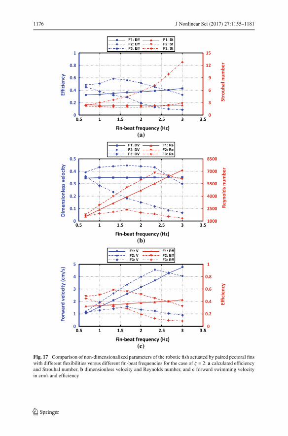
To bring additional insight into the robotic fish performance analysis, one can fur-ther study some non-dimensionalize parameters of the robotic fish. These parametersinclude the Reynolds number, Re = |VC |L
ν, and the Strouhal number St = 2 f S sin γA
|VC| ,where |VC| is the swimming speed of the robot, L is the robotic fish length, ν is thekinematic viscosity of water, S is the pectoral fin span length, γA is the fin flappingamplitude (Sitorus et al. 2009; Kodati et al. 2008), and f is the fin-beat frequency.Another non-dimensionalize parameter of interest is the dimensionless velocity, whichis defined as VDL = |VC|
SωA, where ωA = π
(ζ+1)Tp
. These dimensionless parameters arereported in Fig. 17 for pectoral fins with different flexibilities and ζ = 2, versus dif-ferent fin-beat frequencies. Figure 17a shows a distinct inverse correlation betweenthe efficiency and the Strouhal number. For each fin flexibility, when the Strouhalnumber is at its lowest, the efficiency is highest. Figure 17b shows that the roboticfish demonstrates the highest dimensionless velocity when the Reynolds number is atthe lower end, except for the rigid fin (F1), where the dimensionless velocity remainsalmost constant. Figure 17c shows that the optimal frequency for the forward swim-ming velocity of the robotic fish for each flexible fin does not coincide with the optimalfrequency for the efficiency. Specifically, the frequency for optimal efficiency is lowerthan that for optimal swimming speed. This can be explained as follows. The optimalfrequency for swimming speed is largely dependent on the natural frequency of the
123
1176 J Nonlinear Sci (2017) 27:1155–1181
0
0.2
0.4
0.6
0.8
1
0
3
6
9
12
15
0.5 1 1.5 2 2.5 3 3.5
Fin-beat frequency (Hz)
Stro
uhal
num
ber
Effici
ency
F1: EffF2: EffF3: Eff
F1: StF2: StF3: St
(a)
0.5 1 1.5 2 2.5 3 3.50
0.1
0.2
0.3
0.4
0.5
1000
2500
4000
5500
7000
8500
F1: DVF2: DVF3: DV
F1: ReF2: ReF3: Re
Dim
ensi
onle
ss v
eloc
ity
Reyn
olds
num
ber
Fin-beat frequency (Hz)(b)
0
1
2
3
4
5
0
0.2
0.4
0.6
0.8
1
0.5 1 1.5 2 2.5 3 3.5
Fin-beat frequency (Hz)
Effici
ency
Forw
ard
velo
city
(cm
/s)
F1: VF2: VF3: V
F1: EffF2: EffF3: Eff
(c)
Fig. 17 Comparison of non-dimensionalized parameters of the robotic fish actuated by paired pectoral finswith different flexibilities versus different fin-beat frequencies for the case of ζ = 2: a calculated efficiencyand Strouhal number, b dimensionless velocity and Reynolds number, and c forward swimming velocityin cm/s and efficiency
123

J Nonlinear Sci (2017) 27:1155–1181 1177
fin, at which the fin oscillation amplitude is maximized given a fixed amplitude forthe servo motion. As the actuation frequency is increased (but before reaching thenatural frequency), while the useful work Wb (see Eq. 33) increases due to increasedthrust and forward velocity, the total work Wt (see Eq. 34) increases even faster sincean increasing portion of the hydrodynamic force is oriented in the lateral direction(which does not contribute to Wb). The latter results in the peaking of the mechanicalefficiency prior to reaching the natural frequency. Therefore, the model presented inthis paper can be used as a tool to address an optimal, multi-objective design problem.Note that the Strouhal numbers shown here are higher than 1, which are far from theStrouhal numbers of biological fish, (typically in the range of 0.25–0.5; Triantafyllouand Triantafyllou 1995; Sitorus et al. 2009; Rohr and Fish 2004). The reason is thatthe robotic fish used in this study is driven solely by the pectoral fins, which results inrelatively low forward swimming speeds and thus large Strouhal numbers.
8 Conclusion and Future Work
The goal of thisworkwas to study the impact of the pectoral finflexibility on the roboticfish performance andmechanical efficiency.We introduced a novel dynamicmodel fora robotic fish actuated with paired pectoral fins, where the fin is modeled as multiplerigid elements joined through torsional springs and dampers and blade element theoryis used to calculate the hydrodynamic forces on the elements. The dynamic modelwas validated through experiments conducted on a robotic fish, where the swimmingand turning performance of the robot was measured for fins with different flexibilities(two flexible, one rigid). The model was then used extensively to evaluate the impactsof fin stiffness, fin-beat frequency, and power/recovery stroke speed ratio on robotswimming speed and mechanical efficiency. The analysis reveals the intricate trade-off between objectives (swimming speed versus efficiency) and supports the use ofthe presented model for multi-objective design of fin morphology and control.
There are several directions in which the current work will be continued. First,it is desirable to be able to efficiently solve the fin dynamics for a larger number ofapproximating segments. To this end, wewill investigate approaches to approximatingthe nonlinear dynamics to facilitate numerical solutions. One example is to replacethe sin and cos terms with their Taylor series approximations. Second, this work (see,for example, Fig. 17c) indicates that flexible fins tend to perform better than rigidfins in speed and efficiency at low fin-beat frequencies, while rigid fins do better athigh fin-beat frequencies. It is thus of interest to develop fins with tunable stiffness(Behbahani and Tan 2015) and investigate the control of stiffness in different robotoperating regimes. Third, in this paper we focused on the case of a rigid link betweenthe actuator and the fin base, which necessitates the use of power/recovery stroke speedratio ζ > 1 in order to produce net positive thrust. Our earlier work (Behbahani andTan 2016a, b) shows that, using flexible passive joints, one can achieve net thrust withsymmetric servo motion during power and recovery strokes, which simplifies controlimplementation and potentially offers gain in speed performance. Therefore, as partof our future work, we will investigate jointly designing and optimizing flexible jointsand flexible fins. Finally, in this work we have only considered pectoral fin propulsion.
123

1178 J Nonlinear Sci (2017) 27:1155–1181
While pectoral fin actuation alone is sometimes useful for locomotion or maneuvering(Hasan 2015), in general it is of interest to explore the interactions between the pectoralfins and the (actuated) caudal fin for optimizing the speed and efficiency of the roboticfish.
Acknowledgements The authors would like to gratefully acknowledge Dr. Shahram Pouya for the usefuldiscussion on scaling laws and Mr. John Thon for the technical support on the robotic fish prototype.
References
Alvarado, P.V.Y., Youcef-Toumi, K.: Design of machines with compliant bodies for biomimetic locomotionin liquid environments. J. Dyn. Syst. Meas. Control 128(1), 3–13 (2006)
Anderson, J.M., Streitlien, K., Barrett, D.S., Triantafyllou, M.S.: Oscillating foils of high propulsive effi-ciency. J. Fluid Mech. 360, 41–72 (1998)
Aureli, M., Kopman, V., Porfiri, M.: Free-locomotion of underwater vehicles actuated by ionic polymermetal composites. IEEE-ASME Trans. Mechatron. 15(4), 603–614 (2010)
Banerjee, A., Nagarajan, S.: Efficient simulation of large overall motion of beams undergoing large deflec-tion. Multibody Syst. Dyn. 1(1), 113–126 (1997)
Barbera, G.: Theoretical and experimental analysis of a control system for a vehicle biomimetic “boxfish”.Master’s thesis, University of Padua, Padua (2008)
Behbahani, S.B., Tan, X.: A flexible passive joint for robotic fish pectoral fins: design, dynamic modeling,and experimental results. In: IEEE/RSJ International Conference on Intelligent Robots and Systems(IROS), Chicago, IL, pp. 2832–2838 (2014a)
Behbahani, S.B., Tan, X.: Design and dynamic modeling of a flexible feathering joint for robotic fishpectoral fins. In: ASME Dynamic Systems and Control Conference (DSCC), San Antonio, TX, vol.1, p. V001T05A005 (2014b)
Behbahani, S.B., Tan, X.: Dynamicmodeling of robotic fish caudal fin with electrorheological fluid-enabledtunable stiffness. In: ASME Dynamic Systems and Control Conference (DSCC), Columbus, OH, vol.3, p. V003T49A006 (2015)
Behbahani, S.B., Tan, X.: Bio-inspired flexible joints with passive feathering for robotic fish pectoral fins.Bioinspir. Biomim. 11(3), 036009 (2016a)
Behbahani, S.B., Tan, X.: Design and modeling of flexible passive rowing joints for robotic fish pectoralfins. IEEE Trans. Robot. 32(5), 1119–1132 (2016b)
Behbahani, S.B., Wang, J., Tan, X.: A dynamic model for robotic fish with flexible pectoral fins. In:IEEE/ASME International Conference on Advanced Intelligent Mechatronics (AIM), Wollongong,pp. 1552–1557 (2013)
Blake,R.W.: Themechanics of labriform locomotion I. Labriform locomotion in the angelfish (Pterophyllumeimekei): an analysis of the power stroke. J. Exp. Biol. 82(1), 255–271 (1979)
Blake, R.W.: The mechanics of labriform locomotion: II. An analysis of the recovery stroke and the overallfin-beat cycle propulsive efficiency in the angelfish. J. Exp. Biol. 85(1), 337–342 (1980)
Blake, R.: Fish Locomotion. Cambridge University Press, Cambridge (1983)Chen, Z., Shatara, S., Tan, X.: Modeling of biomimetic robotic fish propelled by an ionic polymer-metal
composite caudal fin. IEEE-ASME Trans. Mechatron. 15(3), 448–459 (2010)Childress, S.: Mechanics of Swimming and Flying. Cambridge Studies in Mathematical Biology (Book 2),
1st edn. Cambridge University Press, Cambridge (1981)Clark, A.J., Tan, X., McKinley, P.K.: Evolutionary multiobjective design of a flexible caudal fin for robotic
fish. Bioinspir. Biomim. 10(6), 065006 (2015)Dong, H., Bozkurttas, M., Mittal, R., Madden, P., Lauder, G.V.: Computational modelling and analysis of
the hydrodynamics of a highly deformable fish pectoral fin. J. Fluid Mech. 645, 345–373 (2010)Du, R., Li, Z., Youcef-Toumi, K., y Alvarado, P.V. (eds.): Robot Fish: Bio-inspired Fishlike Underwater
Robots, 1st edn. Springer, Berlin (2015)Fontanella, J.E., Fish, F.E., Barchi, E.I., Campbell-Malone, R., Nichols, R.H., DiNenno, N.K., Beneski,
J.T.: Two- and three-dimensional geometries of batoids in relation to locomotor mode. J. Exp. Mar.Biol. Ecol. 446, 273–281 (2013)
Fossen, T .I.: Guidance and Control of Ocean Vehicles. Wiley, Hoboken (1994)
123

J Nonlinear Sci (2017) 27:1155–1181 1179
Harper, K.A., Berkemeier, M.D., Grace, S.: Modeling the dynamics of spring-driven oscillating-foil propul-sion. IEEE J. Ocean. Eng. 23(3), 285–296 (1998)
Hasan, H.: Design, development, and modeling of a wirelessly charged robotic fish. Master’s thesis, Michi-gan State University, East Lansing, MI (2015)
Ichiklzaki, T., Yamamoto, I.: Development of robotic fish with various swimming functions. In: Sympo-sium on Underwater Technology and Workshop on Scientific Use of Submarine Cables and RelatedTechnologies, Tokyo, pp. 378–383 (2007)
Ijspeert, A.J., Crespi, A., Ryczko, D., Cabelguen, J.-M.: From swimming to walking with a salamanderrobot driven by a spinal cord model. Science 315(5817), 1416–1420 (2007)
Kanso, E.: Swimming due to transverse shape deformations. J. Fluid Mech. 631, 127–148 (2009)Kanso, E., Marsden, E.J., Rowley, W.C., Melli-Huber, B.J.: Locomotion of articulated bodies in a perfect
fluid. J. Nonlinear Sci. 15(4), 255–289 (2005)Kato, N., Furushima, M.: Pectoral fin model for maneuver of underwater vehicles. In: Symposium on
Autonomous Underwater Vehicle Technology (AUV), Monterey, CA, pp. 49–56 (1996)Kato, N., Inaba, T.: Guidance and control of fish robot with apparatus of pectoral fin motion. In: IEEE
International Conference on Robotics and Automation (ICRA), Leuven, vol. 1, pp. 446–451 (1998)Kato, N., Wicaksono, B., Suzuki, Y.: Development of biology-inspired autonomous underwater vehicle
BASS III with high maneuverability. In: Proceedings of the 2000 International Symposium on Under-water Technology, Tokyo, pp. 84–89 (2000)
Kato, N., Ando, Y., Tomokazu, A., Suzuki, H., Suzumori, K., Kanda, T., Endo, S.: Bio-mechanisms ofswimming and flying. In: Kato, N., Kamimura, S. (eds.) Elastic Pectoral Fin Actuators for BiomimeticUnderwater Vehicles, pp. 271–282. Springer, Tokyo (2008)
Kelly, S.D.: The mechanics and control of robotic locomotion with applications to aquatic vehicles. Ph.D.dissertation, California Institute of Technology, Pasadena California (1998)
Kelly, S.D., Murray, R.M.: Modelling efficient pisciform swimming for control. Int. J. Robust NonlinearControl 10, 217–241 (2000)
Kim, B., Kim, D.-H., Jung, J., Park, J.-O.: A biomimetic undulatory tadpole robot using ionic polymermetalcomposite actuators. Smart Mater. Struct. 14(6), 1579 (2005)
Kodati, P., Hinkle, J., Winn, A., Deng, X.: Microautonomous robotic ostraciiform (MARCO): hydrody-namics, design and fabrication. IEEE Trans. Robot. 24(1), 105–117 (2008)
Kopman, V., Porfiri, M.: Design, modeling, and characterization of a miniature robotic fish for research andeducation in biomimetics and bioinspiration. IEEE/ASME Trans. Mechatron. 18(2), 471–483 (2013)
Kopman, V., Laut, J., Acquaviva, F., Rizzo, A., Porfiri, M.: Dynamic modeling of a robotic fish propelledby a compliant tail. IEEE J. Ocean. Eng 40(1), 209–221 (2015)
Lachat, D., Crespi, A., Ijspeert, A.: BoxyBot: a swimming and crawling fish robot controlled by a cen-tral pattern generator. In: Proceedings of the First IEEE/RAS-EMBS International Conference onBiomedical Robotics and Biomechatronics, BioRob., Pisa, pp. 643–648 (2006)
Lauder, G.V., Drucker, E.G.: Morphology and experimental hydrodynamics of fish fin control surfaces.IEEE J. Oceanic Eng. 29(3), 556–571 (2004)
Lauder, G.V., Madden, P.G.A., Mittal, R., Dong, H., Bozkurttas, M.: Locomotion with flexible propulsors:I. Experimental analysis of pectoral fin swimming in sunfish. Bioinspir. Biomim. 1(4), S25–34 (2006)
Lighthill, M.J.: Large-amplitude elongated-body theory of fish locomotion. Proc. R. Soc. Lond. B: Biol.Sci. 179(1055), 125–138 (1971)
Liu, H., Wassersug, R., Kawachi, K.: A computational fluid dynamics study of tadpole swimming. J. Exp.Biol. 199(6), 1245–1260 (1996)
Liu, J., Dukes, I., Hu, H.: Novel mechatronics design for a robotic fish. In: IEEE/RSJ International Confer-ence on Intelligent Robots and Systems (IROS), Alberta, pp. 807–812 (2005)
Long, J.H.J., Koob, T.J., Irving, K., Combie, K., Engel, V., Livingston, N., Lammert, A., Schumacher, J.:Biomimetic evolutionary analysis: testing the adaptive value of vertebrate tail stiffness in autonomousswimming robots. J. Exp. Biol. 209(23), 4732–4746 (2006)
Low, K.H.: Locomotion and depth control of robotic fish with modular undulating fins. Int. J. Autom.Comput. 3(4), 348–357 (2006)
Low, K.H., Willy, A.: Biomimetic motion planning of an undulating robotic fish fin. J. Vib. Control 12(12),1337–1359 (2006)
Marras, S., Porfiri,M.: Fish and robots swimming together: attraction towards the robot demands biomimeticlocomotion. J. R. Soc. Interface 9(73), 1856–1868 (2012)
123

1180 J Nonlinear Sci (2017) 27:1155–1181
Mason, R.: Fluid locomotion and trajectory planning for shape-changing robots. Ph.D. dissertation, Cali-fornia Institute of Technology, Pasadena California (2003)
Mason, R., Burdick, J.: Construction andmodelling of a carangiform robotic fish. In: Experimental RoboticsVI. Lecture Notes in Control and Information Sciences, vol. 250, pp. 235–242. Springer, London(2000a)
Mason, R., Burdick, J.W.: Experiments in carangiform robotic fish locomotion. In: IEEE InternationalConference on Robotics and Automation (ICRA), San Francisco, CA, vol. 1, pp. 428–435 (2000b)
Melli, J.B., Rowley, C.W., Rufat, D.S.: Motion planning for an articulated body in a perfect planar fluid.SIAM J. Appl. Dyn. Syst. 5(4), 650–669 (2006)
Mittal, R.: Computational modeling in biohydrodynamics: trends, challenges, and recent advances. IEEEJ. Ocean. Eng. 29(3), 595–604 (2004)
Morgansen, K.A., Triplett, B.I., Klein, D.J.: Geometric methods for modeling and control of free-swimmingfin-actuated underwater vehicles. IEEE Trans. Robot. 23(6), 1184–1199 (2007)
Nakashima, M., Ohgishi, N., Ono, K.: A study on the propulsive mechanism of a double jointed fish robotutilizing self-excitation control. JSME Int. J. Ser. C 46(3), 982–990 (2003)
Palmisano, J., Ramamurti, R., Lu, K.-J., Cohen, J., Sandberg, W., Ratna, B.: Design of a biomimeticcontrolled-curvature robotic pectoral fin. In: IEEE International Conference on Robotics and Automa-tion (ICRA), Rome, pp. 966–973 (2007)
Phelan,C., Tangorra, J., Lauder,G.,Hale,M.:Abioroboticmodel of the sunfish pectoral fin for investigationsof fin sensorimotor control. Bioinsp. Biomim. 5(3), 035003 (2010)
Rohr, J.J., Fish, F.E.: Strouhal numbers and optimization of swimming by odontocete cetaceans. J. Exp.Biol. 207(10), 1633–1642 (2004)
Rosenberger, L.J.: Pectoral fin locomotion in batoid fishes: undulation versus oscillation. J. Exp. Biol.204(2), 379–394 (2001)
Sfakiotakis, M., Lane, D., Davies, J.: Review of fish swimming modes for aquatic locomotion. IEEE J.Ocean. Eng. 24(2), 237–252 (1999)
Shoele, K., Zhu, Q.: Numerical simulation of a pectoral fin during labriform swimming. J. Exp. Biol.213(12), 2038–2047 (2010)
Sitorus, P.E., Nazaruddin, Y.Y., Leksono, E., Budiyono, A.: Design and implementation of paired pectoralfins locomotion of labriform fish applied to a fish robot. J. Bionic Eng. 6(1), 37–45 (2009)
Suzuki, H., Kato, N., Suzumori, K.: Load characteristics of mechanical pectoral fin. Exp. Fluids 44(5),759–771 (2007)
Tan, X.: Autonomous robotic fish as mobile sensor platforms: challenges and potential solutions. Mar.Technol. Soc. J. 45(4), 31–40 (2011)
Tangorra, J., Davidson, S., Hunter, I., Madden, P., Lauder, G., Haibo, D., Bozkurttas, M., Mittal, R.: Thedevelopment of a biologically inspired propulsor for unmanned underwater vehicles. IEEE J. Ocean.Eng. 32(3), 533–550 (2007)
Triantafyllou, M.S., Triantafyllou, G.S.: An efficient swimming machine. Sci. Am. 272(3), 64–71 (1995)Triantafyllou, M.S., Triantafyllou, G.S., Yue, D.K.P.: Hydrodynamics of fishlike swimming. Ann. Rev.
Fluid Mech. 32(1), 33–53 (2000)Vogel, S.: Life in Moving Fluids: The Physical Biology of Flow, 2nd edn. Princeton University Press,
Princeton (1994)Wang, J., Tan, X.: A dynamic model for tail-actuated robotic fish with drag coefficient adaptation. Mecha-
tronics 23(6), 659–668 (2013)Wang, J., Tan, X.: Averaging tail-actuated robotic fish dynamics through force and moment scaling. IEEE
Trans. Robot. 31(4), 906–917 (2015)Wang, Z., Hang, G., Li, J., Wang, Y., Xiao, K.: A micro-robot fish with embedded SMA wire actuated
flexible biomimetic fin. Sens. Actuators A: Phys. 144(2), 354–360 (2008)Wang, J., McKinley, P.K., Tan, X.: Dynamic modeling of robotic fish with a base-actuated flexible tail. J.
Dyn. Syst. Meas. Control 137(1), 011004 (2015)Webb, P.W.: Kinematics of pectoral fin propulsion in cymatogaster aggregata. J. Exp. Biol. 59(3), 697–710
(1973)Webb, P.W.: Bulletin, fisheries research board of Canada. In: Hydrodynamics and Energetics of Fish Propul-
sion, vol. 190, pp. 1–159. Department of the Environment, Fisheries and Marine Service, Ottawa(1975)
Yu, J., Tan, M., Wang, S., Chen, E.: Development of a biomimetic robotic fish and its control algorithm.IEEE Trans. Syst. Man Cybern. B, Cybern. 34(4), 1798–1810 (2004)
123

J Nonlinear Sci (2017) 27:1155–1181 1181
Yu, J., Ding, R., Yang, Q., Tan, M., Wang, W., Zhang, J.: On a bio-inspired amphibious robot capable ofmultimodal motion. IEEE/ASME Trans. Mechatron. 17(5), 847–856 (2012)
Zhang, Y.-H., He, J.-H., Yang, J., Zhang, S.-W., Low, K.H.: A computational fluid dynamics (CFD) analysisof an undulatory mechanical fin driven by shape memory alloy. Int. J. Autom. Comput. 3(4), 374–381(2006)
Zhang, F., Ennasr, O., Litchman, E., Tan, X.: Autonomous sampling of water columns using gliding roboticfish: algorithms and harmful algae-sampling experiments. IEEE Syst. J. 10(3), 1271–1281 (2016)
Zhou, C., Tan, M., Gu, N., Cao, Z., Wang, S., Wang, L.: The design and implementation of a biomimeticrobot fish. Int. J. Adv. Robot. Syst. 5(2), 185–192 (2008)
123