rocstar 3 solid propellant rocket simulation …rocstar 3 solid propellant rocket simulation...
TRANSCRIPT

Rocstar 3
Solid Propellant Rocket Simulation Software
User’s Guide
Center for Simulation of Advanced Rockets University of Illinois at Urbana-Champaign
2270 Digital Computer Laboratory Urbana, IL
Rocstar 3 Users Guide 9/17/08

Rocstar 3 Users Guide Page 1
Printed on Date: 9/17/08
Title: Rocstar 3 Users Guide
Author: Robert Fiedler
Subject: Describes the use of the Rocstar 3 Integrated Rocket Simulation Code.
Revision: Rev. 6
Revision History Revision 0: Initial Release for Gen2.0 Revision 1: Update for Gen2.5 (never fully completed) Revision 2: Update for Gen2.6 Revision 3. Major upgrade for Rocstar 3 Revision 4. Documentation Week Dec. 12, 2005 Revision 5. Documentation Week Dec. 15, 2006 Revision 6. Documentation Week Dec. 14, 2007 Revision 7. Documentation Week, Aug. 2008
Effective Date: 8/29/2008

Rocstar 3 Users Guide Page 2
1.0 Introduction
Rocstar 3 is a general-purpose integrated software package for fully coupled, time-dependent fluid/structure/combustion interaction problems. It consists of a suite of physics applications coupled together by means of a powerful integration framework2. All components of Rocstar 3 are designed to run efficiently on massively parallel computers, enabling the use of detailed, science-based physical models in complex 3-D geometries.
Rocstar 3 is the third generation integrated solid propellant rocket simulation package developed at CSAR1. Previous versions of this code were known internally as GEN0, GEN1, GEN2, GEN2.5, and GEN2.6. The term “GEN3” is an obsolete name for Rocstar 3.
This User’s Guide describes how to perform complex simulations with Rocstar 3 on various computer systems, but does not provide extensive documentation of the component codes. For further details on any component, please see the User’s Guide for that individual module. However, in this User’s Guide, we discuss many of the module-specific input parameters required to set up and run a complex simulation.
2.0 Purpose and Methods
2.1 Rocstar Architecture and Components
The diagram below shows the basic architecture of Rocstar 3. A brief description of the specific modules that perform the functions written in each box is given below.
Figure 1. The Rocstar 3 Architecture
Printed on Date: 9/17/08

Rocstar 3 Users Guide Page 3
2.1.1 Problem Set-up
On the left-hand side of Figure 1, the problem-definition tools and the physics solvers are represented by blue boxes (lighter blue for the solvers). The selection of CAD packages is up to the user, as long as the package can output the geometrical information needed by the mesh generator(s). We typically employ Pro/Engineer (http://www.ptc.com/) to produce a CAD description of the fluid and solid domains, and export that information in IGES format (http://www.nist.gov/iges/). However, IGES is known for its lack of portability, and other formats may prove superior, provided the mesh generation tools can understand them.
To some degree, the mesh generator may also be chosen by the user, although the physics application developers have written preprocessors that require mesh and boundary condition information in a very specific format. Our intention is to provide reader routines that support a number of commonly used mesh generators along with the preprocessors for the physics applications, which will allow the user to select any supported meshing tool. Currently, meshes and boundary conditions (BCs) for the fluids codes are prepared using Gridgen (http://www.pointwise.com/), while meshes and BCs for the structural mechanics codes are usually prepared using Patran (http://www.mscsoftware.com/) or Truegrid (http://www.truegrid.com/). However, it is possible to make some complete coupled input data sets using only Gridegen.
Once the meshes and boundary condition information are written in a supported format, the physics application preprocessors can be run either by hand or with the aid of the Rocprep input data set preparation tool. We illustrate the use of Rocprep in chapter 4 of this User’s Guide. The preprocessors create complete input data sets (partitioned for parallel execution) for each physics application.
2.1.2 Physics Applications
The 3 light blue boxes on the lower left in Figure 1 represent the various general-purpose physics solvers that are available for use with Rocstar. The existing fluid dynamics packages are called Rocflu3 and Rocflo4. The basic algorithms in these codes were pioneered by Jameson5. Rocflu operates on unstructured tetrahedral or mixed tetrahedral/hexahedral/pyramid/prism mesh cells to handle complex geometries. An advantage of mixed meshes is the ability to use hexahedral cells to provide high spatial resolution in boundary layers near physical surfaces. The fluid equations are formulated on moving meshes (Arbitrary Lagrangian Eulerian, or ALE scheme) to handle geometrical changes such as propellant burning and deformation. This finite volume code employs a new high order WENO-like approach, as well as the HLLC6 scheme to handle strong transients such as igniter flows. Time integration is accomplished via either the 3rd or 4th order explicit multistage Runge-Kutta time stepping algorithm. A new, non-dissipative version called Rocflu-ND is currently available in Rocstar, and boundary conditions for rocket problems are being implemented and tested. The spatial discretization scheme is second order and the time-stepping scheme is implicit. Low dissipation enables far more accurate solutions for turbulent flows. Note that Rocflu-ND does not yet support turbulence, moving grids, or particles; all of these capabilities are under development. Rocflo uses either the Central Scheme or an upwind scheme involving Roe flux splitting7 on multi-block structured meshes. In addition to explicit Runge-Kutta, Rocflo can use a Dual Time Stepping algorithm to take time steps longer
Printed on Date: 9/17/08

Rocstar 3 Users Guide Page 4
than the Courant (CFL) limit. Both fluid solvers can include turbulence (Rocturb8), Lagrangian superparticles (Rocpart9), smoke (Rocsmoke; equilibrium-Eulerian method10), chemical reactions (Rocspecies), and radiation (Rocrad; flux-limited diffusion approximation). Each of these five plug-in fluid physics modules has a separate User’s Guide.
The rate of propellant deflagration is computed by one of three combustion modules. The physical models are 1-D (normal to the surface) in formulation, but are applied independently at each cell face on the burning propellant surface, making them effectively 3-D. The simplest model, RocburnAPN, adopts the well-known steady burn rate model in which the regression speed is proportional to the local gas pressure raised to the power “n”. Two dynamic burn rate models may also be selected. Both solve a 1-D time-dependent heat conduction equation for the temperature profile in order to capture ignition transients. One of the dynamic models (RocburnZN11) is based on the Zeldovich-Novozhilov approach, while the other (RocburnPY) uses a simpler pyrolysis law. RocburnPY can also compute the heating of the propellant surface by hot igniter gases prior to burning, as well as ignition once the critical temperature is exceeded. A heat-flux look-up table computed by Rocfire, the detailed 3-D propellant combustion simulation code developed at CSAR, can be used by RocburnPY to determine the local instantaneous burn rate based on the propellant formulation12 in a full-system simulation.
Rocstar includes two finite-element structural mechanics solvers, Rocfrac and Rocsolid13. Both solvers feature an ALE formulation to account for the conversion of solid propellant into the gas phase. They handle large strains and rotations, can solve the 3-D heat conduction equation, and include a variety of element types and constitutive models. Rocsolid has an implicit time integration scheme that uses the multigrid method (for problems without burning) and/or BiCGSTAB to solve the required linear systems efficiently in parallel. Rocfrac has an explicit time integration scheme. Rocfrac can include cohesive volumetric finite elements between ordinary elements to follow crack propagation.
2.1.3 Integration Framework and CS Services
The Integration Interface (center of Figure 1) is a library (API) called Roccom2. Roccom facilitates the exchange of data and functions between different modules, including those written in different programming languages (C++, F90). By making a limited number of calls to Roccom routines, the physics applications gain access to a large number of useful components included in our integration framework (column of boxes on the right-hand side of Figure 1).
The orchestration module (red box in Fig. 1) controls the execution of the physics applications, including initialization, coupled time stepping, interface jump conditions, output dumps, and stopping criteria. The available time stepping schemes are described in section 2.2 below. Rocstar retains its legacy Fortran 90 Rocman2 orchestration module via a compilation option, but the default Rocman version is the more sophisticated, generalized, C++ implementation called Rocman3. See section 3.3 below for more details.
The green boxes on the right-hand side of Fig. 1 represent the Rocstar Computer Science service modules. The surface propagation module (Rocprop) computes the motion of the propellant surface as it regresses due to burning. Rocprop can be used in coupled simulations as well as fluids-only or solids-only calculations. It can be switched off for problems in which there is no
Printed on Date: 9/17/08

Rocstar 3 Users Guide Page 5
significant loss of mass from the solid domain (fluid/structure interaction without burning, or evolution times << burn times). Rocprop features two surface propagation algorithms: 1) the older marker particle method, and 2) the face-offsetting method23, a new, efficient, robust, and general surface propagation scheme developed at CSAR by X. Jiao. The face-offsetting method (FOM) is much better at tracking surface motion near edges and corners. FOM first propagates cell faces, where the normal vectors are well defined, and then determines the new locations of cell vertices. Surface features are detected and maintained by solving an eigenvalue problem whose solution indicates the type of feature (corner, edge, or smooth) and uniquely defines the local null (tangent) space on which nodes may be translated to maintain optimal mesh quality without altering the surface shape.
The mesh modification schemes in Rocstar operate at different levels of desperation. Mesh smoothing (without changing the number of mesh vertices) for unstructured meshes is accomplished in the Rocmop module through calls to the Mesquite package, a serial code developed at Sandia National Laboratory14. Each partition calls Mesquite concurrently, providing both real and ghost nodes (on the exterior). Mesquite smoothes only the interior nodes of these mesh partitions, so including the ghost nodes is essential to maintaining mesh quality. After Mesquite smoothes all partitions, the coordinates of real vertices shared by multiple partitions are averaged to ensure that the meshes still match at partition boundaries. It is possible (but not usually necessary) to call Mesquite multiple times to alleviate any impact on mesh quality due to averaging shared nodes. Because the evolution equations in our solvers are formulated on moving grids, no solution transfer is required after mesh smoothing, although the amount that the mesh can change locally per call is evidently limited by a Courant-like stability criterion. Support for non-tetrahedral element types is included in Rocmop using the latest Mesquite version, but we have not yet added support for structured meshes (i.e., Rocflo).
Global remeshing (and, in principle, local mesh repair) can be performed using tools from Simmetrix, a company spun off from Professor Mark Shephard’s group at Rensselaer Polytechnic Institute. The Rocrem module performs serial or parallel off-line remeshing and partitioning, parallel solution transfer from the old mesh to the new mesh, and generation of all input files required to restart a simulation involving Rocflu. There is currently no remeshing support for the other physics solvers. The remeshing process is automated via a batch job script creation tool described in section 6.2. Remeshing can be triggered by small fluid time steps and/or may be performed at scheduled intervals of physical problem time.
Local mesh repair is in a very early stage of development. The Simmetrix tools could be used to repair selected partitions of a mesh, which becomes very important when the entire mesh is too large to fit in memory. Our short-term plan is to pass the repaired mesh to Rocrem as though global remeshing had taken place. In the long term, we hope to save wall clock time by taking advantage of the fact that much of a repaired mesh remains unchanged. Ultimately, we would like to utilize the mesh quality improvement and mesh adaptivity capabilities under development in the ParFUM package (on which Rocrem is based) to perform local mesh repair, rather than relying on Simmetrix.
The solution transfer module called Rocface15 enables the physics applications to exchange interface quantities across non-matching meshes, which is essential to solving coupled fluid/structure interaction problems. The interpolation scheme is exactly conservative by
Printed on Date: 9/17/08

Rocstar 3 Users Guide Page 6
construction, because it operates on an overlay mesh, which is a common refinement of the two meshes on either side of the interface. Each subdivision of the overlay mesh lies entirely within a cell face in both surface meshes. Moreover, interpolation errors are minimized in the least squares sense, leading to a scheme that has been demonstrated to be many times more accurate than other recently published methods16.
Rocstar automatically collects performance data for functions registered with Roccom, including physics application solution update times, data transfer times, output dump write times, etc. More detailed profiling (at the subroutine, loop, or statement level) can be performed by inserting a small number of low-overhead calls to Rocprof into the source code. See the Rocprof User’s Guide for more information.
Asynchronous Parallel I/O can be performed using Rocpanda. Rocpanda designates a user-specified number of processes as I/O servers, which collect data in the form of MPI messages from the compute processes, combine the data, and write it to disk in a manageable number of files in the desired format in the background as the simulation continues17. We have not made much use of this capability recently.
All major input and output by Rocstar is performed using Rocin and Rocout. These modules allow the solvers to perform I/O without regard to the specific file format. The file format to be used in a given simulation may be selected at run time without any changes to the physics modules or their preprocessors. HDF4 format is the default, while CGNS (http://www.cgns.org/) can be selected via a compilation option. Data in either format can be visualized using CSAR’s Rocketeer suite, (http://www.csar.uiuc.edu/F_software/rocketeer/). We persuaded the CGNS committee to extend their standard to support ghost (rind) cells in unstructured meshes. Rocflu CGNS data sets therefore require a visualization tool linked with CGNS version 2.4 or later.
2.1.4 Charm/AMPI
All modules in Rocstar use MPI (Message Passing Interface) to pass messages between partitions. The modules are compatible with AMPI18 (http://charm.cs.uiuc.edu/research/ampi/), an implementation of MPI developed at the University of IL that treats processes as user-level threads. There are two key benefits of AMPI for Rocstar: 1) the AMPI processes are “virtual” so that they can run on any number of physical CPUs, and 2) the virtual processes can be migrated from one CPU to another for dynamic load balancing. In performing large rocket simulations, we have used the first of these two features extensively to utilize available computational resources (fewer processors available than the number of partitions). Thread migration is most effective when the domain is over-decomposed (many more partitions than physical processors). Load balancing via thread migration has been used to improve the parallel efficiency of Rocflo, where the initial structured mesh includes blocks of different sizes. For unstructured meshes, partitioning tools are used on new meshes to balance the load, and therefore further load balancing is not required but can still be beneficial. Dynamic load balancing would become very important if the meshes are ever refined or coarsened differently in each partition, due to either geometrical changes (e.g., propellant burning and deformation) or solution-based mesh adaptation.
Printed on Date: 9/17/08
Rocstar 3 Users Guide Page 7
2.2 Coupled Time Stepping Schemes
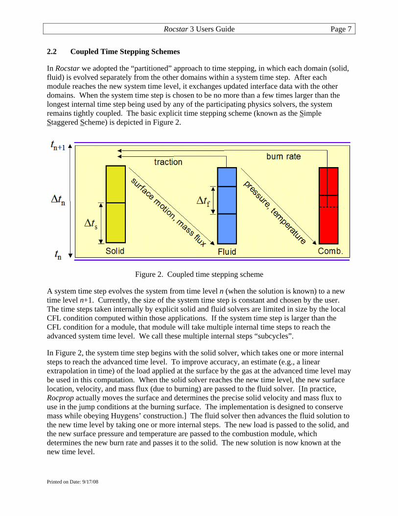
In Rocstar we adopted the “partitioned” approach to time stepping, in which each domain (solid, fluid) is evolved separately from the other domains within a system time step. After each module reaches the new system time level, it exchanges updated interface data with the other domains. When the system time step is chosen to be no more than a few times larger than the longest internal time step being used by any of the participating physics solvers, the system remains tightly coupled. The basic explicit time stepping scheme (known as the Simple Staggered Scheme) is depicted in Figure 2.
Figure 2. Coupled time stepping scheme
A system time step evolves the system from time level n (when the solution is known) to a new time level n+1. Currently, the size of the system time step is constant and chosen by the user. The time steps taken internally by explicit solid and fluid solvers are limited in size by the local CFL condition computed within those applications. If the system time step is larger than the CFL condition for a module, that module will take multiple internal time steps to reach the advanced system time level. We call these multiple internal steps “subcycles”.
In Figure 2, the system time step begins with the solid solver, which takes one or more internal steps to reach the advanced time level. To improve accuracy, an estimate (e.g., a linear extrapolation in time) of the load applied at the surface by the gas at the advanced time level may be used in this computation. When the solid solver reaches the new time level, the new surface location, velocity, and mass flux (due to burning) are passed to the fluid solver. [In practice, Rocprop actually moves the surface and determines the precise solid velocity and mass flux to use in the jump conditions at the burning surface. The implementation is designed to conserve mass while obeying Huygens’ construction.] The fluid solver then advances the fluid solution to the new time level by taking one or more internal steps. The new load is passed to the solid, and the new surface pressure and temperature are passed to the combustion module, which determines the new burn rate and passes it to the solid. The new solution is now known at the new time level.
Printed on Date: 9/17/08
Rocstar 3 Users Guide Page 8
The accuracy and stability of the above explicit time stepping scheme may be improved by repeating the computations required to advance from time level n to level n+1, using the interface values at level n+1 that were obtained in the previous iteration as a better estimate of the burn rate and load on the solid surface at the new time level. We call such iterative improvement “Predictor-Corrector” cycles or iterations. The “Predictor” cycle is the same as the explicit method, while the “Corrector” cycles attempt to reduce the relative and absolute changes in the interface quantities from one iteration to the next to values below prescribed tolerances. P-C iterations are most useful when the implicit solid solver is selected for the simulation.
Additional time stepping schemes have been implemented in Rocman3, including Farhat’s Improved Staggered Scheme (ISS), which should be somewhat more accurate and stable than the SSS scheme without incurring the cost of P-C iterations. It could be the scheme of choice for coupled problems involving Rocfrac, although we have not tested it extensively. A coupling algorithm that includes heat transfer between the fluid and solid domains is also available, but has not been thoroughly tested, either. See section 5 below for details.
3.0 Building Rocstar
This section describes how to build and run Rocstar 3 on various platforms.
3.1 Obtaining the Source Code
The first step is to obtain a user name and password for the CSAR CVS code repository [currently from Mark Brandyberry ([email protected])].
A convenient way to use CVS is to set the CVSROOT environment variable. All examples in this Users Guide are for the C shell (or similar shells). The system prompt is indicated by a “%” here, but may be different on your machine. You can set CVSROOT with the command line:
% setenv CVSROOT :pserver:<username>@galileo.cse.uiuc.edu:/cvsroot
In the line above, substitute <username> for your actual CVS user name. You can add this line to your “.login” configuration file to define it automatically every time you log on to your machine, especially if you do not access other CVS repositories very often.
The first time you access the CSAR CVS server, you must log in to CVS with your signon and password. When you access it again, CVS will find an entry in a file called “.cvspass” in your home directory and will not require a password. If you do not already have a .cvspass file, create an empty one in your home directory via the command:
% touch .cvspass
Now log on to CVS to add the entry to .cvspass:
% cvs login Enter CVS password:
Printed on Date: 9/17/08
Rocstar 3 Users Guide Page 9
Once this command succeeds, you will not be prompted for a password again.
Now you can check out the Rocstar source code and utilities using the command:
% cvs co genx/Codes
This creates a directory “genx/Codes”.
The Rocstar source code directory hierarchy is important to preserve in order for the makefiles to work correctly. The makefiles are compatible with the GNU version of make, called “gmake” on most systems (except for turing.cse.uiuc.edu, where it is called “make”). The GNU version is much more powerful than ordinary Unix “make”; compiling Rocstar without gmake is not possible.
The contents of the genx/Codes directory is shown below:
% ls CSAR_Vis RocfluQ1D RocstarControl.txt CVS RocfluidMP RocstarControl3.txt Makefile Rocfrac Roctail Makefile.basic Rocfrac3 bin Makefile.in Rocman configure README Rocman3 configure.in Rocburn Rocmop lib Roccom Rocpanda patches Rocface Rocprof rocstar.C Rocflo Rocprop utilities Rocflu Rocrem RocfluMP Rocsolid %
Each of the subdirectories (Rocburn, Rocman, etc.) has its own makefile for that specific code. These makefiles are used by the main Rocstar makefile “Makefile.basic” to compile all of the Rosctar modules, so you do not need to build each module by hand.
The Roccom subdirectory contains machine-specific makefiles that set the proper compile options, library locations, etc. for each supported platform:
% cd Roccom % ls -aCF ./ Makefile.Linux Rocin/ ../ Makefile.OSF1 Rocin2/ CVS/ Makefile.SunOS Rocmap/ External/ Makefile.basic Rocout/ Makefile Makefile.common Rocsurf/ Makefile.AIX Makefile.custom include/ Makefile.BlueGene Makefile.dep lib/ Makefile.Charm Makefile.in specs.bgl Makefile.Darwin Rocblas/ src/ Makefile.IRIX64 Rochdf/ %
The makefile “Makefile.common” defines many machine-specific settings for ALL Rocstar modules (not just Roccom) by invoking these machine-specific makefiles. It is possible to
Printed on Date: 9/17/08

Rocstar 3 Users Guide Page 10
change some of the default compilation settings (such as which compiler to use) by modifying “Makefile.custom”, but the user does not normally need to do so.
3.2 Building Charm
Before compiling Rocstar, you must first decide whether to use normal MPI or Charm/AMPI. If you want to run the coupled code on fewer CPUs than there are partitions, or if you need to perform remeshing, you must use Charm. Note that the fluid solvers can distribute multiple partitions per processor, so a fluid-only simulation does not have to be compiled with Charm to run on fewer CPUs than the number of partitions. However, once such a run starts, the number of CPUs used cannot be changed, because the output dumps have the partitions distributed in a certain way. If you do not want to use Charm, or if you are using a system that has a version of Charm installed for all users (such as turing), you may skip the rest of this section.
If you want to use Charm and your system does not already have it installed, you must check out and compile Charm before building Rocstar. To make the process of checking out and compiling Charm easier, use the genx/Codes/utilities/Makecharm script. From your home directory, type:
% <path>/genx/Codes/utilities/Makecharm
where you substitute <path> for the path to your genx directory. Makecharm will log into the Charm group’s CVS server to check out the Charm source code. Makecharm will prompt you for an empty password the first time you connect to their CVS server. Just hit the “Enter” key if that happens. Then Makecharm will get the latest Charm source and archive it in a tar file. Next, Makecharm prompts you for which feature of Charm to build:
up041:~ %~/genx/Codes/utilities/Makecharm cvs checkout: Updating charm U charm/CHANGES U charm/LICENSE . . . cvs checkout: Updating charm/tools/projector/test U charm/tools/projector/test/LogTest.java U charm/tools/projector/test/Makefile Saving clean source as Charm_031505.tgz Enter target (AMPI, ParFUM):
Once you enter AMPI or ParFUM (for remeshing using Rocrem), the Charm source will be compiled if your operating system is supported by Makecharm. If Charm compiles successfully, at the end you should see some lines like the following:
.
.
. AMPI built successfully. Next, try out a sample program like tests/charm++/simplearrayhello up041:~ %
Makecharm can use an existing charm directory, i.e., a fresh source code tree, and it will prompt you for what to do if it finds one in your current directory. Before running Makecharm, you can
Printed on Date: 9/17/08

Rocstar 3 Users Guide Page 11
optionally obtain the most recent source code version that is known to build and run test cases successfully on your type of system from http://charm.cs.uiuc.edu/autobuild/cur/. On the LLNL ASC platforms, where different systems share home directories, you will want to specify a charm directory name other than “charm” when Makecharm prompts you for the name, for example, enter “charm_<hostname>”, to distinguish this build from builds for other hosts. Note that you cannot subsequently change the locations of libraries and executables built with dynamic linking (including charm) because the paths get “hard-coded” into the binaries. Therefore, you cannot change those directory names later without breaking the installation.
3.3 Compiling Rocstar
To build Rocstar, you need to run gmake in the genx/Codes directory. By default, the executable is called “genx/Codes/bin/rocstar”. Again, the dynamically linked libraries cannot be moved after they are built. The user can choose which fluid, combustion, and solid solvers to use at run time (see section 4) – all of them are compiled.
The following commonly used options, which apply to all modules, can be included on the gmake command line:
• all, util, help, clean These are targets for the makefiles; the default is “all”, which builds the rocstar executable plus the prep tools. The “util” target builds only the prep tools. The “clean” target removes all object codes, libraries, and executables in preparation for another compilation.
• -j <n> Use n processes to build in parallel. It is best if n is less than or equal to the number of CPUs on the node you are using for compilation.
• CHARM=1 Compile with Charm/AMPI. Default is without charm.
• CHARM_PATH=<charm install directory> Give path to Charm installation directory. This is particularly useful on LLNL systems, where machines of different architecture share home directories and so you need separate builds. Default is $HOME/charm.
• PREFIX=<prefix_dir> Specify parent directory for the bin and lib subdirectories that will contain the Rocstar executable and dynamically linked libraries. Default is the genx/Codes directory. This option is useful in building more than one executable from the same source tree, e.g., to compare performance of AMPI vs. MPI.
• OBJECT_MODE=<32|64> Selects 32 or 64-bit addressing. On the IBM SP, the default is 32, but we highly recommend using 64. You can issue the command:
% setenv OBJECT_MODE 64
before compiling anything. We recommend that you put this line in your .cshrc file to use 64-bit mode at all times. On MacOS and turing Linux, the default mode is 64.
Printed on Date: 9/17/08

Rocstar 3 Users Guide Page 12
• REMESH=1 Enable Remeshing by building Rocrem and other stand-alone tools. Default is without remeshing. You must also compile with charm, after building the ParFUM target, not just AMPI. You can run a simulation with a build of Rocstar that did not specify CHARM=1 or REMESH=1, but you need to compile with these options to produce the remeshing tools.
• SIMMETRIX=1 Use Simmetrix software for remeshing operations. Note that Simmetrix is supported only on turing (MacOS), alc, zeus, and blackrose (AMD/Intel Linux, not turing Linux).
• SIMMETRIX_PATH= <path> Path to Simmetrix binary library files (top level), if not building on turing.
• AMR=1 Enable AutoMatic Remeshing. You need the SIMMETRIX and CHARM flags (build with ParFUM), but REMESH=1 is implied by AMR=1. Currently, there is no advantage in using this option, because the batch job script will handle remeshing. After remeshing, if compiled with AMR=1, Rocstar will attempt a "warm restart" (restart of Rocstar without exiting the simulation). This is not the most robust option, however; instead, use the pj_all_ar batch job script creation tool (see Section 6).
The following option selects the desired version of the orchestration module:
• ROCMAN=ROCMAN2 Use the older Fortran version of Rocman in place of the new Rocman3. Default is to use the new Rocman. As explained below, the format of the Rocstar and Rocman control files are different for different Rocman versions. There is no known advantage to using version 2 of Rocman.
The following option controls data formats that can be read/written by Rocin/Rocout:
• CGNS=1 Compile and link the CGNS file format library, in addition to HDF.
The following option selects the desired version of Rocmop for mesh smoothing; (default version is Rocmop 1):
• ROCMOP=ROCMOP2 With this version, you do not need to create 2 layers of ghost cells for Rocflu meshes; Rocmop 2 takes care of that for you. Unfortunately, this version suffers from memory leaks and other problems (worse than version 1) that we have been unable to resolve. Note that when you remesh, 2 layers of ghost cells will be created for you, and then there is no particular advantage to using version 2.
The following options for the gmake command line are for debugging and tuning purposes:
• DEBUG=1 With debugging. Default is without debug information.
Printed on Date: 9/17/08

Rocstar 3 Users Guide Page 13
• NOOPT=1 Turn off optimization, but do not include symbolic information (like DEBUG=1 would do). Default is to compile with optimization enabled. Some compilers have trouble including symbolic information.
• EFENCE=1 With Electric Fence. Default is without Electric Fence. This tool works on a limited number of architectures, including Linux.
• LIBSUF=a Static Linking. Rocstar by default is built using dynamically linked libraries stored in the <PREFIX>/lib directory. This will create two executables, rocstar_flo and rocstar_flu, because the fluids codes use common name spaces and cannot coexist. The statically linked executables should work even if moved to different directories. Note that some systems do not support dynamic linking very well, and so you are forced to build with static linking.
• ROCPROF=1 Enable Rocprof for detailed profiling. Default is without Rocprof. See section 7.2.1 below for details on how to use Rocprof.
The new, implicit, non-dissipative version of Rocflu, known as both RocfluMP and Rocflu-ND, can be selected on the gmake command line:
• ROCFLU=RocfluMP Enable RocfluMP. Default is to use the original Rocflu. Before compiling, you must apply a code patch. For further instructions, see genx/Codes/patches/RocfluMP2Rocstar.readme.
Rocflo and Rocflu physics options are also selected on the gmake command line:
• TURB=1 Enable turbulence. Default is no turbulence.
• STATS=1 Enable statistics collection (used with particles or turbulence) in separate text files. Default is no statitstics.
• PLAG=1 Enable Lagrangian superparticles. Default is no particles.
• PEUL=1 Enable smoke (Equilibrium Euleriean). Default is no smoke.
Typical compilation uses a command line such as (use “make” in place of gmake on turing):
up041:~/gen3/genx/Codes % gmake –j 2 CHARM=1 CHARMDIR=$HOME/charm_up TURB=1 STATS=1 \ PREFIX=$HOME/gen3_up/genx_charm_turb
This compiles the code using 2 CPUs, selects Charm/AMPI, enables turbulence modeling with statistics collection, and places the executables in ~/gen3_up/genx_charm_turb/bin. If the build is successful, the following executable programs will exist in the bin directory:
up041:~/gen3_up/genx_charm_turb/bin % ls addpconn hdf2vtk rfloprep rfracprep surfdiver autosurfer makeflo rfluinit rhpm surfextractor charmrun profane rflumap rocstar surfjumper hdf2plt rfctest rflupart rsolidprep up041:~/gen3/genxc/bin %
Printed on Date: 9/17/08
Rocstar 3 Users Guide Page 14
Along with rocstar, you get the file format translators hdf2plt and hdf2vtk. The hdf2plt translator can be used to convert hdf output files to plt format for visualization with Tecplot. Most of the remaining executables are prep tools.
The <PREFIX>/lib directory will contain 17 dynamically linked libraries (*.so):
up041:~/gen3_up/genx_charm_turb/lib % ls libRHDF4.so libRoccomf.a libRocfrac.so libRocmop.so libRocprop.so libRocblas.so libRocface.so libRocin.so libRocout.so libRocsolid.so libRocburn.so libRocflo.so libRocman.so libRocpanda.so libRocsurf.so libRoccom.so libRocflu.so libRocmap.so libRocprof.so libmetis.a up041:~/gen3/genxc/lib %
You should make sure that all 17 *.so libraries were actually produced during the compilation. On turing, you will see a set of *.dylib files, which are links to the corresponding *.so libraries. The presence of rocstar is not sufficient to indicate successful completion of the build. If any of these libraries is missing one or more routines, you will get an error message referring to that library (perhaps that the library is “not found”) at run time.
3.4 Separate Object Code Directories
It is possible to create a separate directory tree to store object codes produced when compiling Rocstar. This can be useful for those who want to build the code in different ways from the same source code tree without cleaning everything out in between compiles. To accomplish this goal, first create the object code directory and cd to it:
% mkdir <obj_dir> ; cd <obj_dir>
In the above line, substitute <obj_dir> with the desired object code directory name. Next, use the configure script:
% <path>/genx/Codes/configure --prefix=<exe_dir>
In the above line, substitute <path> with the path to your genx/Codes directory, and substitute <exe_dir> with the name of the directory in which to put the bin and lib subdirectories that will contain the rocstar executable and libraries (not the object codes). The configure script will create a new Codes directory tree under <obj_dir>, but it will contain only makefiles customized with the specified source code, bin, and lib paths.
3.5 Building Rocstar with Separate Object Code Directories
If you to use the “configure” script to set up separate object code directions as described in the previous section, you may also specify where to put the executables and libraries. To build Rocstar under a directory other than the source tree, create a build directory, say "foo" (or any other name), cd to "foo", and then invoke the configure script in this directory with its relative path or absolute path, like:
/path-to/configure --prefix=<PREFIX>
Printed on Date: 9/17/08

Rocstar 3 Users Guide Page 15
--prefix is used to specify an installation directory (default is the current directory). Configure generates Makefiles and the build directory tree structure under "foo". Now customize foo/Roccom/Makefile.custom if desired, and then run "gmake" under directory foo with normal command-line options. The precedence of the PREFIX definition is:
Highest: gmake command-line option PREFIX=<PREFIX>, which overwrites
Medium: Makefile.custom definition PREFIX=<PREFIX>, which overwrites
Lowest: configure option --prefix=<PREFIX>.
3.6 External Libraries
The Rocstar makefiles support many platforms; however, some library paths may need to be changed if you are trying to compile the code on an unsupported system or wish to use your own version of a library. For example, the HDF (version 4) libraries are often not installed in standard places, and even if they are, they may not have been compiled thread-safe (-fPIC compiler option) or they may refer to missing routines. The HDF library (libdf.a) and its dependent libraries (jpeg, zlib, and szip) are not supplied with the Rocstar distribution, but precompiled binaries and source codes can be obtained from http://hdf.ncsa.uiuc.edu. The Rocstar makefiles attempt to find the HDF libraries in several standard places (and a few non-standard ones) and set the HDF_PATH variable. If the HDF libraries are not found, genx/Codes/Roccom/Makefile.custom will need to be modified to correctly set the HDF_PATH variable. The HDF library libdf.a and its dependent libraries libjpeg.a, libz.a, and possibly libszip.a must be available, or Rocstar will not compile. There is an entry in the makefiles to look for them in $HOME/HDF. If necessary download and install the precompiled libraries in your home directory under a directory called ‘HDF/lib’. The include files go in HDF/include. There are separate tar files for HDF, jpeg, zlib, and szip. There is also a script genx/Codes/utilities/build_HDF to help you build all these libraries from the source codes on various platforms.
4.0 Preparing Rocstar Input Data Sets
Describing how to create CAD models and produce meshes with appropriate boundary condition information using Gridgen, Patran, or Truegrid is beyond the scope of this Users Guide. However, we have produced a number of CAD models and grids that can be used by a new Rocstar user to gain experience performing a variety of simulations with the code.
A number of module-specific preprocessor programs are compiled along with Rocstar. These preprocessors are used by the Rocstar data set preprocessor “Rocprep” to create Rocstar input data sets. Below we give a brief tutorial on how to use Rocprep; for more complete information, see the Rocprep Users Guide.
To use Rocprep, you must check it out from CVS (it does not come with the Rocstar source code):
Printed on Date: 9/17/08

Rocstar 3 Users Guide Page 16
% cvs co Rocstar/Rocprep/Codes
This will create Rocstar/Rocprep/Codes in your current directory, which will contain a set of perl scripts that comprise Rocprep.
Rocprep gets its data from one of the Rocstar Native Data Archives (NDAs) available on turing in /turing/projects/csar/NDAs. Export controlled datasets are stored in a separate directory. The NDAs include a number of rocket-simulation and test-case data files, each with one or more mesh and input parameter file sets. These file sets consist of files produced by the meshing tools mentioned in section 2.1.1, as well as text input parameter files for each physics application, described in some detail below. Different sets of grid files in the Archives under a given simulation name are referred to as “Grid1”, “Grid2”, etc. The different sets of text input data files are referred to as “Data1”, “Data2”, and so on. Note that the numbering of the Grid and Data file sets are independent of each other; you may be able to use Grid2 with Data1, for example. The directories in the NDAs contain README files describing the particular problem, geometry, mesh, boundary conditions, physics options, etc.
Assuming you have access to the NDAs, begin creating a Rocstar input data set from them by running Rocprep with no arguments to see the usage information:
% Rocstar/Rocprep/Codes/Rocprep.pm First switch must be mode switch -A|C|E|P|U, not: **************************************************************************** Usage: Rocprep.pm -A|C|E|P [OPTION]... Major modes of operation: -A, --all extract and preprocess -C, --check check an existing dataset at -d <path> -E, --extract copy NDA files to target at -t <path> -P, --preprocess run module preptools on data at -d <path> Physics module options: -o [m] [n] Rocflo preprocessing, optional NDA Data<m> & Grid<n> dirs -u [m] [n] Rocflu preprocessing, optional NDA Data<m> & Grid<n> dirs -f [m] [n] Rocfrac preprocessing, optional NDA Data<m> & Grid<n> dirs -s [m] [n] Rocsolid preprocessing, optional NDA Data<m> & Grid<n> dirs -b Rocburn preprocessing Module-specific flags: -r <m> specify <m> regions (rocflu only), default is -n value -splitaxis <n> force split along n=0,1, or 2 axis (rocflo only) -un <units> convert model units to meters (rocfrac only) General options: -i <o|u|f|s> surfdive interface meshes, default infers from physics options -d <path> path to source data, default is current working directory -h, --help print this help message and terminate -n <m> specify <m> processors/partitions -t <path> target path for new rocstar dataset -p <path> path to preptool binaries, default will use shell path -x, --ignore ignore RocprepControl.txt control file Example: Rocprep.pm -A -o 1 1 -f 2 4 -d archiveDir/ -t newDataset/ -n 8 **************************************************************************** %
Printed on Date: 9/17/08

Rocstar 3 Users Guide Page 17
The –splitaxis option (if used) is passed to the makeflo structured mesh partitioner to control how the fluid domain is partitioned.
The –un option is passed to the Rocfrac preprocessor and is interpreted as a conversion factor for the unit of length. For example, some solid models in the NDAs are in inches or millimeters and need to be scaled by a factor of 0.0254 m/in or 0.001 m/mm, respectively.
As an example of Rocprep’s usage, suppose you wanted to simulate the “lab scale rocket”. This problem is called “labscale” in the NDAs. Suppose further that you want to use Rocflo, RocburnAPN, and Rocfrac on the coarsest available meshes. According to the README files, the coarsest meshes are called Grid1 under both the labscale/Rocflo and labscale/Rocfrac NDA subdirectories. Note that the Rocburn directories are under the labscale/Rocstar subdirectory; these are very short text files which require no actual preprocessing. Rocprep simply copies all Rocburn input directories that it finds.
You can create the Rocstar dataset using:
% Rocprep.pm -A -o 1 1 -f 1 1 -d /csar/NDAs/labscale -t 016procs –p ~/genx/Codes/bin -n 16 *************************************************************************** Rocprep Tool Version 1.0 For Rocstar Version 3.0 File formats Center for Simulation of Advanced Rockets University of Illinois, Urbana, IL 61801 www.csar.uiuc.edu Code Authors: Mark Brandyberry ([email protected]) Court McLay ([email protected]) *************************************************************************** Wed Mar 16 15:48:55 2005: Rocprep Initialized ALL = 1 BINDIR = IGNOREFILE = 0 NUMPROCS = 16 ROCBURN = 1 ROCBURNAPN = 0 ROCBURNPY = 0 ROCBURNZN = 0 ROCFLO = 1 ROCFLODATA = Data1 ROCFLOGRID = Grid1 ROCFLOROCFRAC = 1 ROCFLOROCSOLID = 0 ROCFLU = 0 ROCFLUROCFRAC = 0 ROCFLUROCSOLID = 0 ROCFRAC = 1 ROCFRACDATA = Data1 ROCFRACGRID = Grid1 ROCPREPVERS = 1.0 ROCSOLID = 0 ROCSTARVERS = 3.0
Printed on Date: 9/17/08

Rocstar 3 Users Guide Page 18
SOURCEDIR = /csar/NDAs/labscale/ TARGETDIR = /home/rfiedler/lab_coarse/016procs/ Wed Mar 16 15:48:55 2005: Checking NDA files Ending phase: Check NDA Files for module RocfloProcessor. Ending phase: Check NDA Files for module RocfracProcessor. *************************************************************************** Wed Mar 16 15:48:55 2005: Extracting NDA files to rocstar dataset Ending phase: Extract NDA Files for module RocfloProcessor. Ending phase: Extract NDA Files for module RocfracProcessor. *************************************************************************** Wed Mar 16 15:48:56 2005: Running preprocessor codes to make rocstar dataset /home/rfiedler/gen3/genx/Codes/bin/makeflo labscale-PLOT3D.grd 16 labscale.top labscale.grda > /home/rfiedler/lab_coarse/016procs//makeflo.log 2>&1 Ending phase: Run Preprocessors for module RocfloProcessor. Ending phase: Run Preprocessors for module RocfracProcessor. Ending phase: Run Preprocessors for module RocfaceProcessor. *************************************************************************** Wed Mar 16 15:49:13 2005: Checking rocstar dataset files for consistency Ending phase: Check Rocstar Dataset Files for module RocfloProcessor. Ending phase: Check Rocstar Dataset Files for module RocfracProcessor. Ending phase: Check Rocstar Dataset Files for module RocfaceProcessor. *************************************************************************** *************************************************************************** Run terminated with error: NO ERRORS *************************************************************************** %
No errors were reported, so the files were successfully extracted, preprocessed, and partitioned. The overlay mesh for interface data transfer by Rocface was successfully created. Figure 3 sketches the Rocstar input data set directories (blue text) and files created by Rocprep. The green text color indicates files that Rocstar generates during a simulation.
Printed on Date: 9/17/08

Rocstar 3 Users Guide Page 19
RocmopRocmopControl.txt
Figure 3. Rocstar run directory hierarchy
We will describe many of the text input parameters in the section 5. It is important to note here that a handful of the fluid input parameters affect the initial solution and/or the number of ghost cell layers, and must therefore be chosen BEFORE preprocessing. To accomplish this, you would first extract the files from the NDA by using Rocprep with the “-E” option, edit the parameter files, and then run Rocprep again, this time with the “-P” option to perform the preprocessing. In this case, you should specify “-d ./016procs” for the source files, rather than an NDA directory, since you want to use the native data files that you have just modified.
5.0 Input Files
In this section, we describe the key input parameters for Rocstar, as well as those for several of the physics applications. For complete details on the physics application input files, see the corresponding User’s Guides. Refer to Figure 3 above for the locations of these files within a Rocstar run directory.
Each physics application has its own control file, as does Rocstar itself, plus Rocman , Rocmop, Rocout, and Rocpanda. The contents of each control file can be quite different from other control files.
Printed on Date: 9/17/08

Rocstar 3 Users Guide Page 20
5.1 RocstarControl.txt
This is the main control file for any Rocstar simulation. Two formats exist, corresponding to the old and new Rocman orchestration module versions. The contents of each are described below. Note that Rocman3 is the default, and Rocman 2 is no longer used much; however, some of the NDAs contain old format files. You can use the convertall utility in genx/Codes/Rocman3/util to convert old Rocstar and Rocman format control files to the new formats after preprocessing or extracting files with Rocprep. They create new files (with “.new” appended to the names), which must be renamed to replace the existing, old format ones. A more convenient way to convert these two files is via the script genx/Codes/utilities/converter3, which drives the conversion utilities, saves your original files, and renames the new versions. This script is run in a Rocstar run directory and takes the parent directory of Rocman3/util as an optional argument.
5.1.1 Rocman3 Format
Rocman3 is the default version. Rocstar must be compiled with the ROCMAN=Rocman2 option on the command line to use the old file formats. Below is a representative RocstarControl.txt:
CouplingScheme = "SolidFluidBurnSPC" FluidModule = "Rocflo" SolidModule = "Rocsolid" BurnModule = "RocburnAPN" OutputModule = "Rocout" InitialTime = 0 MaximumTime = 2.0 MaxNumPredCorrCycles = 1 MaxNumTimeSteps = 10000000 TolerTract = 0.001 TolerMass = 0.001 TolerVelo = 0.001 TolerDisp = 0.001 CurrentTimeStep = 5.0e-05 ZoomFactor = 1 OutputIntervalTime = 1.0e-03 MaxWallTime = 4704000 ProfileDir = "Rocman/Profiles"
Coupling schemes currently supported currently include:
FluidAlone (Fluid alone without combustion, i.e., no calls to Rocburn)
FluidBurnAlone (Fluid alone with combustion)
SolidAlone (Solid alone without combustion)
SolidFluidSPC (Solid, fluid, no comb., simple staggered scheme with P-C)
Printed on Date: 9/17/08

Rocstar 3 Users Guide Page 21
SolidFluidBurnSPC (Fluid, solid, comb., simple staggered scheme with P-C)
SolidFluidBurnEnergySPC (SolidFluidBurnSPC plus heat transfer)
FluidSolidISS (Fluid, solid, no comb., Improved Staggered Scheme)
The available physics modules were described briefly in section 2.1.2. The fluid solver is Rocflo or Rocflu. The solid solver is Rocfrac or Rocsolid. Even if you are running a fluid-only simulation, you must pick either Rocfrac or Rocsolid as the solid solver, even though it will not be used at all. The combustion mode is one of: RocburnAPN, RocburnPY, or RocburnZN. The output mode can be either Rocpanda or Rocout. Rocpanda was described in section 2.1.3. It also has its own control file in the Rocman subdirectory, which will be generated automatically by the pj_all script described in section 6. Choosing Rocout here causes each compute process to write its own set of output files. The I/O is still performed concurrently, but the simulation must wait for the write operations for a given dump to complete before resuming the computation. Note also that the use of Rocout results in the creation of 1 output file per process. For large simulations, hundreds of thousands of files are written, and the use of wildcard characters to refer to them often results in “word too long” errors from various Unix commands. Note that Rocpanda has not been used extensively with Rocstar 3, and is not compatible with Charm. InitialTime, MaximumTime
These entries give the beginning physical problem time (in seconds), and the maximum physical problem time (in seconds). In the example, the simulation will start at zero seconds, and will stop at 2.0 seconds. To restart a simulation that has not reached the desired final time, the initial time must be set > 0. In this case, Rocstar will read Restart.txt to find the last output time, and will restart from the corresponding output dump. Restart.txt also contains the system time step number corresponding to the physical problem times.
MaxNumPrecCorrCycles, MaxNumTimeSteps
The first of these 2 parameters gives the maximum number of Predictor-Corrector cycles allowed. A value of 1 means that no Corrector iterations are to be done; this corresponds to the explicit coupled time stepping scheme. We recommend allowing no more than 6 P-C cycles. The second parameter is the maximum number of system time steps allowed. We typically set it to a huge value, since the simulation will either reach the final time or encounter some numerical problem before it reaches the maximum number of steps. Specifying smaller step limits is mostly used for benchmarking purposes.
TolerTract, TolerMass, TolerVelo, TolerDisp
These tolerances are the convergence criteria for interface quantities during Predictor-Corrector cycles. They are compared to the L2 norms of the differences in the tractions, mass density, velocity magnitude, and displacement magnitude from one cycle to the next. Extensive experimentation with different values has not been done, but loose tolerances would affect the order of convergence as well as the accuracy of the coupling scheme.
Printed on Date: 9/17/08

Rocstar 3 Users Guide Page 22
CurrentTimeStep, ZoomFactor
The current timestep value sets the system timestep (in seconds) for the simulation. The zoom factor is a means of accelerating the slowest time scale in rocket problems (the propellant burn-back time)24. For a rocket motor under quasi-steady operating conditions, the evolution is governed by the change in surface area due to burning, and the regression rate can be accelerated to make the propellant burn back more quickly in the simulation than it actually does without changing the numerical solution (e.g., the pressure history) very much. Rocflu (only) has a “time zooming” formulation of the fluid equations that modifies the injected mass flux and adds source terms designed to recover the evolution that occurs for the nominal burn rate. Set the zoom factor to 0 for no propellant regression (although mass may still be injected at the burning surface); set it to 1 for normal burn-back (even if the solid domain is not part of the simulation; Rocprop moves the surface according to the burn rate from Rocburn), and set it to values > 1 to accelerate the burn-back time scale by that factor.
OutputIntervalTime
This parameter sets the physical problem time interval (in seconds) between output dumps. Shoot for a few hundred dumps per simulation for smooth animations.
MaxWallTime
The maximum wall clock time in seconds that the job is allowed run. Computations will stop at this wall clock time and the code will complete its final output before exiting. Allow extra time in the job submission script for final file writing.
ProfileDir
The name of the directory where the performance timing data files should be placed. This directory should already exist, and the path should be relative to the Rocstar run directory. If this parameter is not specified or the directory does not exist, the timing files will be written in the Rocstar run directory.
5.1.2 Old Rocman Format
This format is practically obsolete, and certainly less human-readable than the current format.
FullyCoupled Rocflo Rocfrac RocburnAPN Rocout 0.0, 0.1 1, 1000000 0.001, 0.001, 0.001, 0.001 1.0e-06, 1. 1.0e-04 3600.0 Rocman/Profiles/ READ(UNIT=UnitCoupling,FMT=*) mWin, fWin, sWin, bWin, ioWin READ(UNIT=UnitCoupling,FMT=*) InitialTime, MaximumTime READ(UNIT=UnitCoupling,FMT=*) MaxNumPrecCorrCycles, MaxNumTimeSteps READ(UNIT=UnitCoupling,FMT=*) TolerTract, TolerMass, TolerVelo, TolerDisp
Printed on Date: 9/17/08

Rocstar 3 Users Guide Page 23
READ(UNIT=UnitCoupling,FMT=*) CurrentTimeStep, ZoomFactor READ(UNIT=UnitCoupling,FMT=*) OutputIntervalTime READ(UNIT=UnitCoupling,FMT=*) MaxWallTime READ(UNIT=UnitCoupling,FMT='(A)') GENXTimingDataDir Rocman modes: BareBone, FluidAlone, SolidAlone, or FullyCoupled Fluids modes: Rocflo, RocfloDummy, Rocflu, or RocfluDummy Solids modes: Rocfrac, RocfracDummy, Rocsolid, or RocsolidDummy Burn modes: RocburnAPN, RocburnPY, or RocburnZN
The text after Rocman/Profiles/ are comments describing the parameters. It shows the FORTRAN read statements (with variable names) that read each line in the file.
The first line of the file specifies the coupling mode, physics solvers, and output module: <coupling mode> <fluid solver> <solid solver> <combustion module> <output mode> The coupling mode can be one of the following:
1. BareBone: Loads no computational modules and hence requires no input data. This is useful only for debugging the driver and checking the system environment.
2. FluidAlone: Loads only fluid and combustion modules (i.e., no solids).
3. SolidAlone: Loads only solid modules (i.e., no fluids or combustion).
4. FullyCoupled: Loads fluids, solids, and combustion modules.
5.2 RocmanControl.txt
The Rocman control file affects numerous aspects of integrated simulations. For the old and new versions of Rocman, the content of the control file is similar. Although the name remains the same, the formats are quite different. Both formats are described below. Here we describe the content.
The order of interpolation refers to the extrapolation (or interpolation for Corrector cycles) used to compute interface quantities at the advanced time level, as described in section 2.2.
Either the pressure (scalar, no sheer forces) or the full traction vector including sheer forces can (in principle) be passed from the fluid to the solid. It is computationally less expensive to pass the pressure, and doing so is an accurate approximation for flows having high Reynolds numbers (low viscosity). Passing tractions is not implemented in Rocstar3. The ambient pressure is an optional value (the default is 0) that will be subtracted from the fluid pressure in computing the load on the solid. It can be set to the initial uniform pressure or a boundary value for the fluid domain, but it does not impose values for the fluid variables. It can be useful in problems such as the super-seismic shock, where the very high initial gas pressure by itself (not the shock)
Printed on Date: 9/17/08

Rocstar 3 Users Guide Page 24
would otherwise drive a spurious wave into the solid. It is also useful for simulating such things as arteries, where again the initial fluid pressure would significantly deform the solid in a manner that detracts from the intended physical problem.
The solid density in this control file is be used solely for fluid-only problems. It affects the mass injection rate at the burning propellant surface. For fully-coupled problems, the solid solver provides the solid density.
We have not explored using different values for the data transfer parameters very much.
The face-offsetting surface propagation scheme can be enabled in this file by replacing the “F” with a “T” at the beginning of the appropriate line. We recommend using Face-Offsetting in all simulations.
Asynchronous input and output here refers to Rocpanda. We are just beginning to test this in Rocstar 3.
5.2.1 Rocman3 Format
The new format for RocmanControl.txt must be used with Rocman3 (the default version):
# Rocman verbosity Verbose = 0 # write output hdf files into separate <rank> directories Separate_out = 0 # order of interpolation InterpolationOrder = 1 # 1 for no sheer, 2 for with sheer TractionMode = 1 # ambient pressure subtracted from fluid pressure at interface P_ambient = 0
# Solid density for fluid-alone mode, pressure and burn-rate for solid-alone mode Rhoc = 1703.0 Pressure = 6.8e+6 BurnRate = 0.01
# Data transfer parameters: verbose level, order of quadrature rules, max iterations, # tolerance for iterative solver RFC_verb = 1 RFC_order = 2 RFC_iteration = 100 RFC_tolerance = 1.e-6
# Whether to enable face-offsetting Face-offsetting = T # Number of surface smoothing iterations PROP_rediter = 1
Printed on Date: 9/17/08

Rocstar 3 Users Guide Page 25
# Whether to use asynchronous input and output AsyncInput = F AsyncOutput = F
Avoid using the “d” format for double precision exponents, such as 6.8d6. The C++ language does not handle that like Fortran does.
Separate_out should be set to 1 only on machines like BlueGene/L, where the number of files in a single output dump is too large for the file system to handle. You would want to use a special set of scripts to create all of these directories conveniently.
5.2.2 Old Rocman Format
The old format must be used with the old Rocman. You would have to build Rocstar with ROCMAN=Rocman2 to use this. There is no good reason to use Rocman2 instead of Rocman3.
1 # Order of interpolation 1, 8.501e6 # Traction mode (1=pressure, 2=tractions), ambient pressure 1703.0 # Solid density for fluid-alone mode 1 2 100 1.e-6 # Data transfer parameters: verbose level, order of quadrature rules, max iterations , tolerance for iterative solver F # Whether to enable face-offsetting F F # Whether to use asynchronous input and output
5.3 RocmopControl.txt
The optional Rocmop/RocmopControl.txt file controls mesh smoothing via Rocmop:
1 #verbosity 0 #method 0 #lazy 165.0 #tolerance 0.0 #maxdisp 3 #N 0.0 #disp threshold
At verbosity level 1, Rocstar will report when Rocmop is called. At level 2, you will get messages about entering and leaving various Rocmop routines. Default is 0, which is eerily silent in that you cannot tell whether any smoothing is occurring.
Parameter “method” selects the smoothing algorithm. Use “0” for Mesquite, which is the default method.
The “lazy” option evaluates mesh quality every call, but does not smooth the mesh unless the quality is worse than that indicated by the tolerance parameter. Default is 0, which means to smooth on every call without bothering to compute mesh quality. Computing the mesh quality is relatively expensive compared to smoothing, so we always set lazy to 0.
Parameter “tolerance” is the value of the mesh quality measure beyond which smoothing is triggered if the lazy option is enabled. Default is 165 degrees for the maximum dihedral angle.
Printed on Date: 9/17/08

Rocstar 3 Users Guide Page 26
We are exploring other mesh quality measures, or perhaps normalizing them to have a range from 0 to 1, where 1 is good.
Parameter “maxdisp” is the maximum displacement due to smoothing allowed for any node per one smoothing call. If Mesquite wants to make large changes in the mesh, you may need to limit the amount of change per time step to avoid generating a bad solution in the calling physics application (i.e., Rocflu). You want to avoid moving nodes more than a fraction of one “local element linear dimension”. Note that if the domain is deforming rapidly and you limit the displacements too much, the elements along the domain surface will get very distorted. Limiting displacements is useful primarily when the mesh smoother is improving a “poor input mesh”. Default is 0, which means do not limit the motion of nodes.
If bad solutions are reported by Rocflu when the motion of nodes is not limited, and turning off mesh smoothing (by setting N to 0; see below) eliminates the bad solution (until mesh quality becomes poor), setting maxdisp to a non-zero value may solve the problem. Try setting maxdisp to at least 10 times the surface motion speed times the typical fluid timestep. For example, if the burn rate ~ 0.01 m/s, and the fluid time step ~ 10-6 s, set maxdisp = 10-7 m or larger. If time zooming is being used, increase maxdisp by at least a factor of Z.
Parameter “N” is the number of calls to wait before performing smoothing. Default is 1, which means to smooth every step. A value of 0 disables smoothing. A value of 2 means to smooth on every other call. One can save a lot of wall clock time by setting N between 2 and 5 if smoothing takes a significant fraction of the run time. For N higher than 5, the nodes may change position too much for the physics solvers to get a stable solution – you could overcome this by limiting the displacements, but this is not recommended. Nonzero values for maxdisp are not recommended for N > 1 (you should use smaller values of N), although doing so might speed up a computation considerably.
Parameter “disp threshold” is intended to trigger smoothing when the physics surface nodes have moved by more than the specified amount (compared to the previous smoothing). This has not proven to be a useful option in many situations.
5.4 RocinControl.txt and RocoutControl.txt
The control files for Rocin and Rocout are both optional. If present in the Rocman subdirectory, they have 2 important entries: format = <format> prefix = <path to input/output dump tree> where <format> is to be replaced by either hdf or CGNS. The default is hdf. It is possible to use hdf format for input and CGNS format for output in the same Rocstar run. Using a non-default prefix for input/output directories can be useful in at least the following two situations, although this is not commonly done: 1) You can use it to write output to local disks on a cluster, such as turing; or 2) you can store the input data in your (permanent) home directory while writing output to some scratch partition with lots of space.
Printed on Date: 9/17/08
Rocstar 3 Users Guide Page 27
5.4 RocpandaControl.txt
The RocpandaControl.txt contains information needed for the operation of the Rocpanda module. Its format is:
C 16 S 2 M 1 D . d B 230
C is the number of compute processes, S is the number of Panda servers (I/O processes), M indicates whether the servers should be distributed across the nodes in a round-robin fashion (M 1, which is the preferred method) or block-wise (M 0), D is normally the directory in which the code runs (leave this parameter as “.”; see the Rocpanda User’s Guide for details), and B is the size of the buffer to use (default is 230 MB); this is currently ignored, since Rocpanda can now determine how much memory is available.
Note: Make sure that you do not leave any extra returns (i.e., blank lines) after the B 230 parameter. Rocpanda will try to read another parameter, fail, and crash. Note also that the pj_all batch file generation script (section 6) will create this file for you automatically.
Again, note that Rocpanda has not been tested much with Rocstar 3.
5.5 Rocface files
The Rocface input files are in a subdirectory under Rocman called <fluid solver><solid solver>. These files are produced by the surfdiver utility program, which is run automatically for you by Rocprep. There is a set of overlay mesh (*sdv.hdf) files and a set of feature detection (*fea*.hdf) files for the fluid and the solid surfaces. Both sets of hdf (or CGNS) files can be visualized. The input surface meshes in the solver Rocin subdirectories can also be visualized, which can be useful for determining whether or not the geometries and BCs in the fluid and solid domains agree at the interface (e.g., when surfdiver fails to construct the overlay mesh).
5.6 Rocburn files
Rocburn requires one file as input; however, that file differs in both name and content depending upon whether you are using the APN, ZN, or PY models. The Rocburn input file is placed at the root of the Rocburn<version> directory (where <version> is APN, ZN, or PY), and is named Rocburn<version>Control.txt.
These control files contain a variety of physical data that Rocburn needs to perform its simulations. They specify one parameter per line with a descriptive comment following the parameter on the same line. See the Rocburn User’s Guides for further information on producing each type of file and the meaning of the parameters.
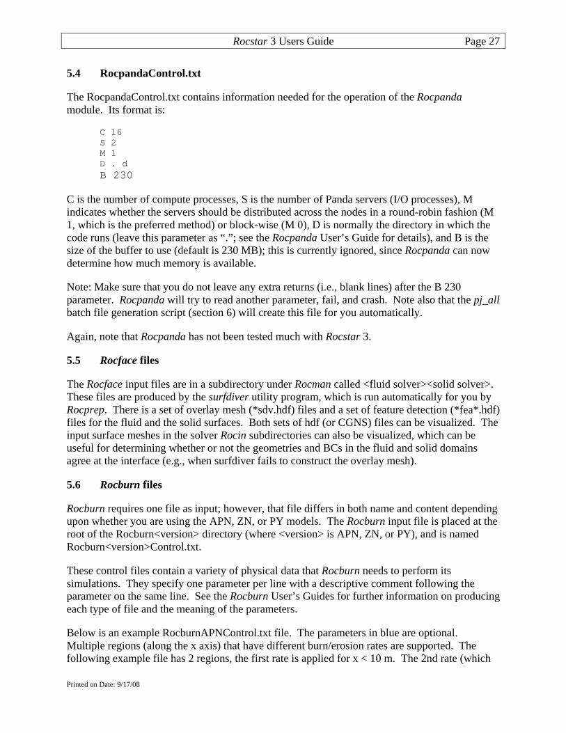
Below is an example RocburnAPNControl.txt file. The parameters in blue are optional. Multiple regions (along the x axis) that have different burn/erosion rates are supported. The following example file has 2 regions, the first rate is applied for x < 10 m. The 2nd rate (which
Printed on Date: 9/17/08
Rocstar 3 Users Guide Page 28
might correspond to an eroding nozzle) extends from 10 to 20 m. RocburnAPN stops reading when the first character in a line is not a number.
0.07696 a in rb=a*P^n, rb in cm/sec and P in atm, a_p (cm/sec) 0.461 n in rb=a*P^n, rb in cm/sec and P in atm, n_p 1 Maximum_number_of_spatial_nodes,_nxmax 2850.0 adiabatic flame temperature, Tf_adiabatic (K) 300.00 initial (deep in propellant) temperature, To_read (K) 1.0e+01 Maximum x value for this material 0.5 a in rb=a*P^n, rb in cm/sec and P in atm, a_p (cm/sec) 0.0 n in rb=a*P^n, rb in cm/sec and P in atm, n_p 1 Maximum_number_of_spatial_nodes,_nxmax 1930.0 adiabatic flame temperature, Tf_adiabatic (K) 300.00 initial temperature, To_read (K) 2.0e+01 Maximum x value for this material Rocburn_2D_Output/Rocburn_APN
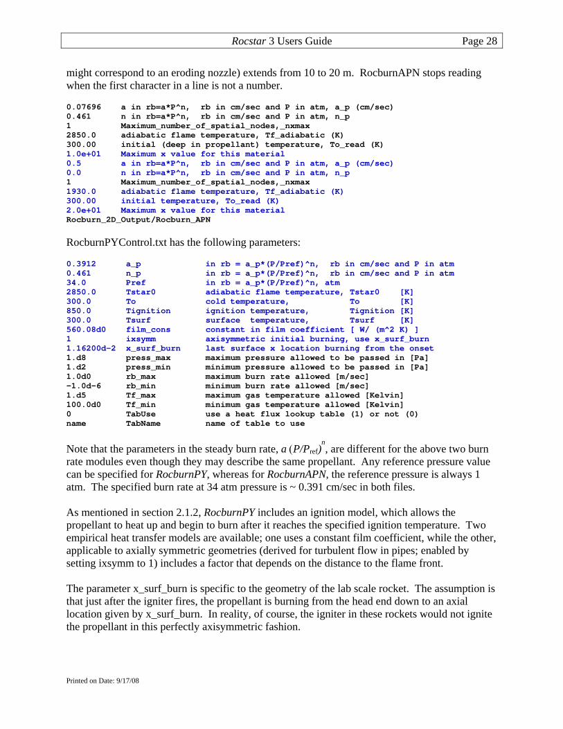
RocburnPYControl.txt has the following parameters:
0.3912 a_p in rb = a_p*(P/Pref)^n, rb in cm/sec and P in atm 0.461 n_p in rb = a_p*(P/Pref)^n, rb in cm/sec and P in atm 34.0 Pref in rb = a_p*(P/Pref)^n, atm 2850.0 Tstar0 adiabatic flame temperature, Tstar0 [K] 300.0 To cold temperature, To [K] 850.0 Tignition ignition temperature, Tignition [K] 300.0 Tsurf surface temperature, Tsurf [K] 560.08d0 film_cons constant in film coefficient [ W/ (m^2 K) ] 1 ixsymm axisymmetric initial burning, use x_surf_burn 1.16200d-2 x_surf_burn last surface x location burning from the onset 1.d8 press_max maximum pressure allowed to be passed in [Pa] 1.d2 press_min minimum pressure allowed to be passed in [Pa] 1.0d0 rb_max maximum burn rate allowed [m/sec] -1.0d-6 rb_min minimum burn rate allowed [m/sec] 1.d5 Tf_max maximum gas temperature allowed [Kelvin] 100.0d0 Tf_min minimum gas temperature allowed [Kelvin] 0 TabUse use a heat flux lookup table (1) or not (0) name TabName name of table to use
Note that the parameters in the steady burn rate, a (P/Pref)n, are different for the above two burn
rate modules even though they may describe the same propellant. Any reference pressure value can be specified for RocburnPY, whereas for RocburnAPN, the reference pressure is always 1 atm. The specified burn rate at 34 atm pressure is ~ 0.391 cm/sec in both files. As mentioned in section 2.1.2, RocburnPY includes an ignition model, which allows the propellant to heat up and begin to burn after it reaches the specified ignition temperature. Two empirical heat transfer models are available; one uses a constant film coefficient, while the other, applicable to axially symmetric geometries (derived for turbulent flow in pipes; enabled by setting ixsymm to 1) includes a factor that depends on the distance to the flame front. The parameter x_surf_burn is specific to the geometry of the lab scale rocket. The assumption is that just after the igniter fires, the propellant is burning from the head end down to an axial location given by x_surf_burn. In reality, of course, the igniter in these rockets would not ignite the propellant in this perfectly axisymmetric fashion.
Printed on Date: 9/17/08
Rocstar 3 Users Guide Page 29
The last two RocburnPY parameters allow you to use a heat-flux lookup table populated with results from detailed 3-D propellant burn simulations performed by Rocfire. 5.7 Rocflo Files
5.7.1 RocfloControl.txt
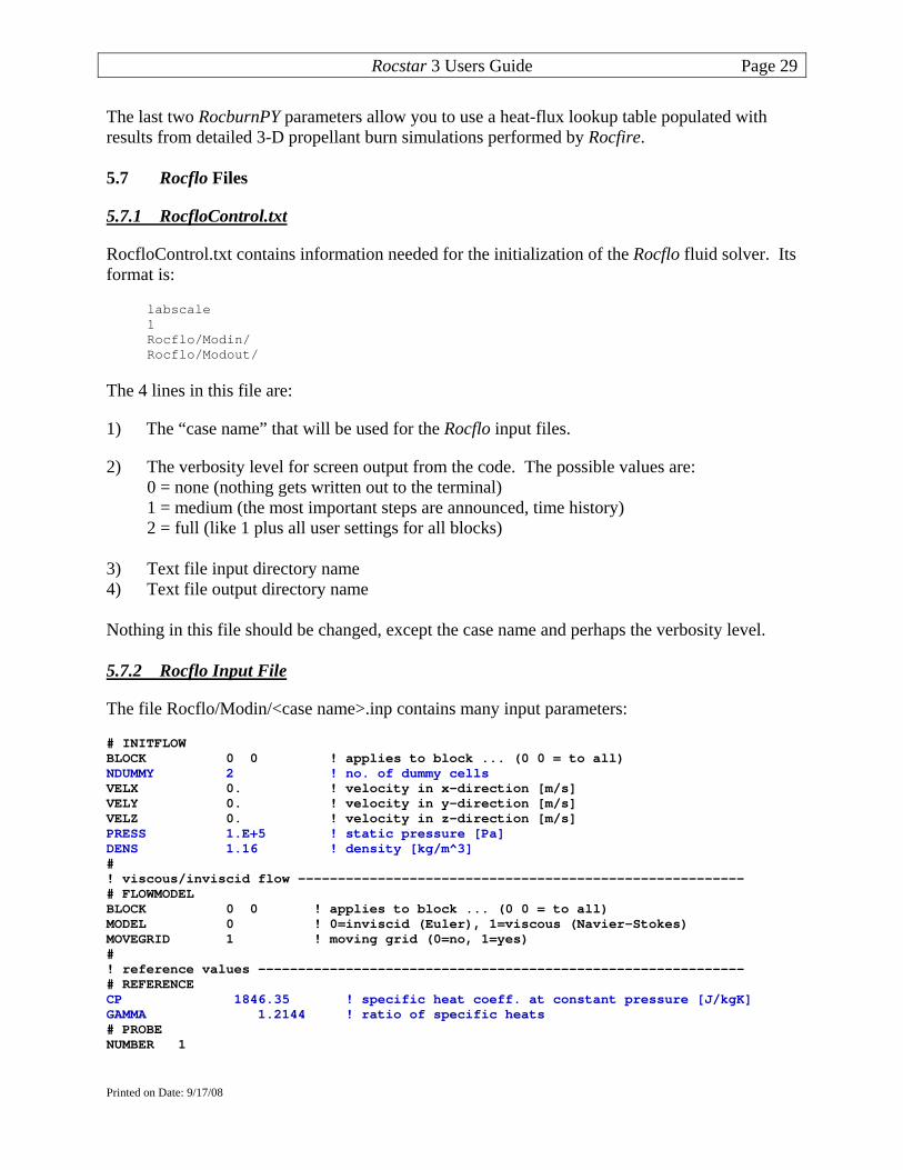
RocfloControl.txt contains information needed for the initialization of the Rocflo fluid solver. Its format is:
labscale 1 Rocflo/Modin/ Rocflo/Modout/
The 4 lines in this file are:
1) The “case name” that will be used for the Rocflo input files.
2) The verbosity level for screen output from the code. The possible values are: 0 = none (nothing gets written out to the terminal) 1 = medium (the most important steps are announced, time history) 2 = full (like 1 plus all user settings for all blocks)
3) Text file input directory name 4) Text file output directory name Nothing in this file should be changed, except the case name and perhaps the verbosity level. 5.7.2 Rocflo Input File
The file Rocflo/Modin/<case name>.inp contains many input parameters:
# INITFLOW BLOCK 0 0 ! applies to block ... (0 0 = to all) NDUMMY 2 ! no. of dummy cells VELX 0. ! velocity in x-direction [m/s] VELY 0. ! velocity in y-direction [m/s] VELZ 0. ! velocity in z-direction [m/s] PRESS 1.E+5 ! static pressure [Pa] DENS 1.16 ! density [kg/m^3] # ! viscous/inviscid flow -------------------------------------------------------- # FLOWMODEL BLOCK 0 0 ! applies to block ... (0 0 = to all) MODEL 0 ! 0=inviscid (Euler), 1=viscous (Navier-Stokes) MOVEGRID 1 ! moving grid (0=no, 1=yes) # ! reference values ------------------------------------------------------------- # REFERENCE CP 1846.35 ! specific heat coeff. at constant pressure [J/kgK] GAMMA 1.2144 ! ratio of specific heats # PROBE NUMBER 1
Printed on Date: 9/17/08

Rocstar 3 Users Guide Page 30
0 0. 0. 0. ! Use coordinates to specify probe location # ! multi-physics modules: ------------------------------------------------------- # TURBULENCE BLOCK 0 0 ! applies to block ... (0 0 = to all) MODEL 0 ! 0=laminar, 1=... # # CONPART BLOCK 0 0 ! applies to block ... (0 0 = to all) USED 0 ! 0=module not used # # DISPART BLOCK 0 0 ! applies to block ... (0 0 = to all) USED 0 ! 0=module not used # # TIMESTEP FLOWTYPE 1 ! 0=steady flow, 1=unsteady flow TIMESTEP 1.E-4 ! max. physical time step [s] WRITIME 2.E-2 ! time offset [s] to store solution PRNTIME 1.E-5 ! time offset [s] to print convergence SOLVERTYPE 0 ! 0=explicit, 1=implicit RKSCHEME 1 ! 1 - classical RK4, 2 - low-storage Wray RK3 # # NUMERICS BLOCK 0 0 ! applies to block ... (0 0 = to all) CFL 3.0 ! CFL number SMOOCF -0.7 ! coefficient of implicit residual smoothing (<0 - no smooth.) DISCR 0 ! type of space discretization (0=central, 1=Roe, 2=MAPS) K2 0.5 ! dissipation coefficient k2 (if discr=0) 1/K4 128. ! dissipation coefficient 1/k4 (if discr=0) ORDER 2 ! 1=first-order, 2=second-order, 4=fourth-order PSWTYPE 0 ! 0=standard pressure switch, 1=TVD type (if discr=0) PSWOMEGA 0.1 ! blending coefficient for PSWTYPE=1 (if discr=0) LIMFAC 5.0 ! limiter coefficient (if discr=1) ENTROPY 0.05 ! entropy correction coefficient (if discr=1)
Note that the parameters in blue affect the initial state and therefore must be chosen BEFORE preprocessing with Roprep.
Note that probe locations can be set using coordinates, if the first of the 4 numbers on the probe line is 0. Probes save values of variables at the nearest cell center every “WRITIME” seconds of physical problem time.
Note that if you want to use turbulence, Lagrangian particles (DISPART), and/or smoke (CONPART), rocstar must also be compiled with TURB=1, PART=1, and/or PEUL=1, as discussed in section 3.3.
Note that the most accurate turbulence models require 3 layers of ghost cells (NDUMMY=3), but not all meshes will allow this many layers.
5.7.2 Boundary Condition File
There are two issues to be aware of related to boundary conditions prescribed in the Rocflo file <case name>.bc:
Printed on Date: 9/17/08

Rocstar 3 Users Guide Page 31
1) If you are using RocburnPY and MFRATE is set to a non-zero value for any patch, that patch will be burning from the outset, injecting that much mass per second per square meter. 2) Time dependent boundary conditions, e.g., for mass injection are not compatible with propellant surfaces controlled by Rocburn. Time dependent conditions must only be prescribed on “non-interacting” surfaces, which is how the igniter is modeled in the RSRM.
5.8 Rocflu Files
5.8.1 RocfluControl.txt
The RocfluControl.txt contains information needed for the initialization of the Rocflu fluid solver. Its format is:
labscale Rocflu/Modin Rocflu/Modout Rocflu/Rocin 1 1
The 6 lines in this file are:
1) The “case name” that will be used for the Rocflu input files (can be a different name from that used by Rocflo or other codes).
2) The path to the text input file directory, relative to the Rocstar run directory.
3) The path where the Rocflu-specific text output files will be placed (not the HDF solution files, which will be placed in the Rocflu/Rocout directory automatically). This includes the probe files, etc.
4) The path to the HDF input file directory, relative to the Rocstar run directory.
5) The verbosity level for screen output from the code.
6) The “checking level” used for the run.
See the Rocflu users manual for the possible values and definitions of the verbosity and checking levels for Rocflu.
5.8.2 Rocflu Input File
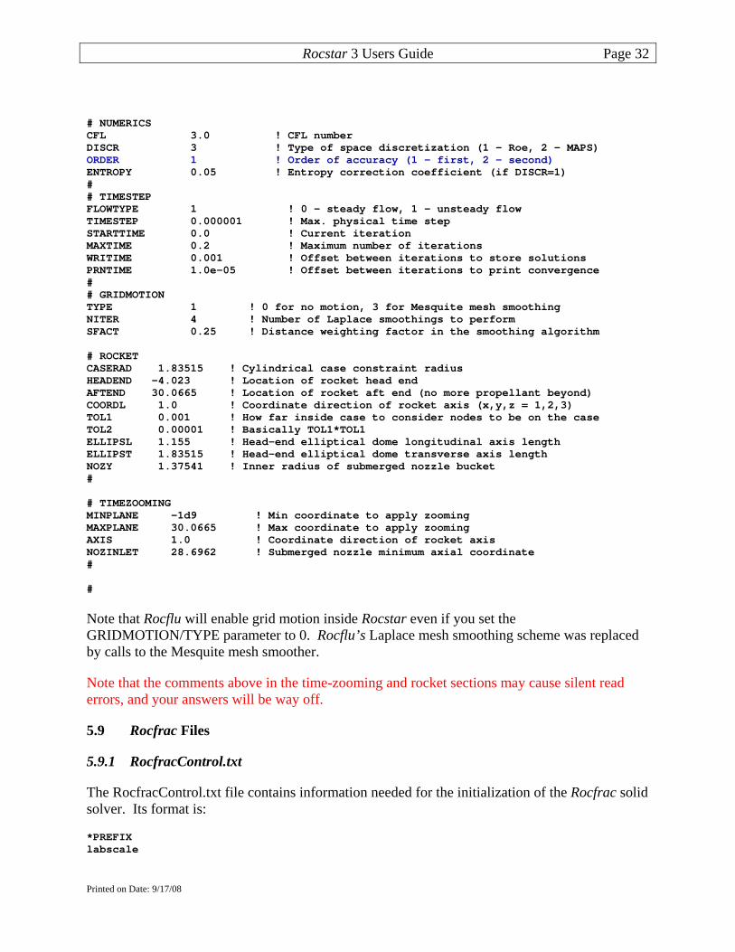
The Rocflu <case name>.inp file shares many of the same parameters with those in Rocflo’s <case name>.inp file. However, the NDUMMY parameter is replaced by an ORDER parameter which determines the stencil size and therefore must be set BEFORE preprocessing with Rocprep. Note that the solver is several times slower for second order accuracy compared to first order. In order to obtain best results from volume mesh smoothing with Rocmop, preprocess with ORDER=2. Reset ORDER to 1 for the simulation.
Printed on Date: 9/17/08
Rocstar 3 Users Guide Page 32
# NUMERICS CFL 3.0 ! CFL number DISCR 3 ! Type of space discretization (1 - Roe, 2 - MAPS) ORDER 1 ! Order of accuracy (1 - first, 2 - second) ENTROPY 0.05 ! Entropy correction coefficient (if DISCR=1) # # TIMESTEP FLOWTYPE 1 ! 0 - steady flow, 1 - unsteady flow TIMESTEP 0.000001 ! Max. physical time step STARTTIME 0.0 ! Current iteration MAXTIME 0.2 ! Maximum number of iterations WRITIME 0.001 ! Offset between iterations to store solutions PRNTIME 1.0e-05 ! Offset between iterations to print convergence # # GRIDMOTION TYPE 1 ! 0 for no motion, 3 for Mesquite mesh smoothing NITER 4 ! Number of Laplace smoothings to perform SFACT 0.25 ! Distance weighting factor in the smoothing algorithm # ROCKET CASERAD 1.83515 ! Cylindrical case constraint radius HEADEND -4.023 ! Location of rocket head end AFTEND 30.0665 ! Location of rocket aft end (no more propellant beyond) COORDL 1.0 ! Coordinate direction of rocket axis (x,y,z = 1,2,3) TOL1 0.001 ! How far inside case to consider nodes to be on the case TOL2 0.00001 ! Basically TOL1*TOL1 ELLIPSL 1.155 ! Head-end elliptical dome longitudinal axis length ELLIPST 1.83515 ! Head-end elliptical dome transverse axis length NOZY 1.37541 ! Inner radius of submerged nozzle bucket # # TIMEZOOMING MINPLANE -1d9 ! Min coordinate to apply zooming MAXPLANE 30.0665 ! Max coordinate to apply zooming AXIS 1.0 ! Coordinate direction of rocket axis NOZINLET 28.6962 ! Submerged nozzle minimum axial coordinate # #
Note that Rocflu will enable grid motion inside Rocstar even if you set the GRIDMOTION/TYPE parameter to 0. Rocflu’s Laplace mesh smoothing scheme was replaced by calls to the Mesquite mesh smoother.
Note that the comments above in the time-zooming and rocket sections may cause silent read errors, and your answers will be way off.
5.9 Rocfrac Files
5.9.1 RocfracControl.txt
The RocfracControl.txt file contains information needed for the initialization of the Rocfrac solid solver. Its format is:
*PREFIX labscale
Printed on Date: 9/17/08

Rocstar 3 Users Guide Page 33
** *DYNAMIC, SCALE FACTOR = 0.25 ** ** Select the 4-node tetrahedral ** *ELEMENT,TYPE=V3D4 ** ** HYPERELASTIC, ARRUDA-BOYCE or NEOHOOKINC ** Young's Modulus, Poisson's Ratio, Density, Expansion Coeffs ** *HYPERELASTIC, ARRUDA-BOYCE 1 6.585e6 0.499 1770.0 0.0 ** FOR ALE:Uncomment next two lines and change Scale Factor = 0.25 *ALE 0.15
Note that the element type you can use depends on the nature of the grid files in the Native Data Archive.
Note also that ALE (regression) can be turned off by commenting out (“**”) the line containing ALE and the line below that, which is an internal mesh motion parameter. Rocfrac requires its internal mesh motion to be enabled only when regression is allowed to occur; deformation is handled by mapping the deformed configuration onto the undeformed space, where the equations of motion are actually solved.
Be sure that the zoom factor in RocstarControl.txt is non-zero if you have ALE enabled here.
5.9 Rocsolid Files
5.9.1 RocsolidControl.txt
The RocsolidControl.txt file contains information needed for the initialization of the Rocsolid solid solver. Its format is:
Scalability test ! Title 1 1 3 4 256 ! NumElemGroup, NumMatSets, NumDof, NumMeshes, BlockSize 1 3 3 4 1.0E-3 100 ! Multigrid Variables (Gamma, NumPreRelax, NumPostRelax, NumMGMeshes, MGtol, MGMaxCycle) 1.0E-4 1000 ! PCGtol, PCGMaxCycle JACOBI ! Preconditioner NEWTON ! Nonlinear solver (Newton or Arc-length) 1 1.0E-4 10 ! NumLoadSteps, NewtonTol, NewtonMax LUMPED ! MassMatrix (Lumped or Consistent) MULTIGRID ! EquationSolver BICGSTAB ! MeshMotionEquationSolver porous_viscoelastic ! MaterialModel propellant ! Material Name 0.929E6 3.604E6 ! ShearMod, TotalShearMod 3447E6 ! TotalBulkMod 0.305 ! TimeConstant 0.02 ! InitialProsity 1770. ! Density b8_ld ! ElementType (b8_ld, b8_bbar, b8_ale, b8_me)
Printed on Date: 9/17/08

Rocstar 3 Users Guide Page 34
Since Rocsolid uses the multigrid method for problems without regression, a number of parameters (blue) in this file depend on the mesh in the Native Data Archive. Moreover, you must use certain element types with certain constitutive models. If regression is enabled in RocmanControl.txt via a non-zero zoom factor, be sure to use an ALE element (e.g., b8_ale) here.
5.9.1 Extracting Input Data From a Used Run Directory
You can use the genx/Codes/utilities/tar_input script to make a tar file containing only the Rocstar input data in a Rocstar run directory. This is very useful for moving input data sets to other machines or creating additional copies of the same input data set for doing parameter study runs concurrently. To use it, your run directory name should adopt the “<problem name>/<nnn>procs” naming convention used here. Do not use tar_input in a Rocstar run directory with a running job, because it temporarily changes the names of the Rocout and Modout subdirectories.
6.0 Running Batch Jobs
6.1 Using pj_all
The genx/Codes/utilities/pj_all script is a powerful utility for preparing and submitting batch jobs to run Rocstar on a number of supported systems. To use pj_all, cd to the directory that contains the Rocstar bin and lib subdirectories, and type (the full path to) pj_all. The script will prompt you for values of a number of key parameters pertaining to the simulations.
Below is an example session, which submits a batch job to run the lab scale rocket. We have already compiled Rocstar and used Rocprep to create the Rocstar run directory. The Rocstar executable is in our home directory under gen3/genx_charm/bin. Note that we have defined an environment variable:
% setenv G30D /turing/projects/rfiedler/gen3-data
and put the Rocstar run directory in $G30D/labscale/016procs to help pj_all find it. This is not absolutely necessary, but it saves typing some full path names. The script also checks the G300 and G301 environment variables (in that order), so you can have datasets on multiple file systems.
In the example below, we typed in only what is colored red:
turing-3:~/gen3_latest/genx_linux% pj_all Found rocstar, rocstar_flo, and/or rocstar_flu To use a different executable, enter PREFIX (full path to parent of Rocstar bin/ directory; default = /turing/home/rfiedler/gen3_latest/genx_linux): [Enter] Enter number of (virtual) compute CPUs (2): 16 Enter problem name (default = Scalability): labscale Enter GEN3 run directory name (default = /turing/projects/csar/rfiedler/gen3-data/labscale/016procs): [Enter] Enter output module (o = Rocout, p = Rocpanda, default = Rocout): [Enter] Enter total number of physical CPUs (16): [Enter] 15 minutes will be reserved for final output
Printed on Date: 9/17/08

Rocstar 3 Users Guide Page 35
Enter total wall clock time limit in minutes (20): [Enter] Enter program name (default = rocstar): [Enter] Which fluid solver? (Rocflo = o, Rocflu = u, default = Rocflo): [Enter] Enter the desired coupling mode. Choose from: SolidFluidSPC SolidFluidBurnSPC SolidFluidBurnEnergySPC FluidSolidISS FluidBurnAlone FluidAlone SolidAlone (default = SolidFluidBurnSPC): [Enter] Which solid solver? (Rocfrac = f, Rocsolid = s, default = Rocfrac): [Enter] Which combustion module? (RocburnAPN = a, RocburnPY = p, RocburnZN = z, default = RocburnAPN): [Enter] Enter system time step (1.0e-05): [Enter] Using Time_step = 1.0e-05 Enter zoom factor (default = 1.): [Enter] Using Zoom_factor = 1. Enter number of P-C iterations (default = 1): [Enter] Enter physical problem end time (1.0e-04): 1.0e-03 Enter output interval (1.0e-03): 1.0e-04 Enter job name (labscale): lab Enter restart mode (new run = 0, restart now = 1, dependent = job ID; default = 0): [Enter] Starting a new run from time t = 0 How many identical jobs to submit (1): [Enter] Do you wish to view the job script? (n): [Enter] Do you wish to submit the job(s)? (y/n/e[xempt]/[e]x[pedite]/i[nteractive]): [Enter] qsub pjob_16p 17070.ada.turing.uiuc.edu turing-2:~/gen3_test/genx_turb%
Note that pj_all gets most of its default values from what it finds in the parameter files in the Rocstar run directory, and therefore the default values you see can differ from those in the example above and from one invocation of the script to the next (if a simulation ran during the interim).
The batch job script that pj_all creates (called “pjob_16p” here) will edit RocstarControl.txt, and if necessary create a RocpandaControl.txt file. A timing data directory named 016procs_timing_turing will be created in the parent directory of the Rocstar run directory. The name depends on the number of CPUs and the machine name.
Early in the example, we set the number of virtual and physical CPUs to use. These numbers can be different only for a Rocstar executable built with CHARM=1. We also chose not to use Rocpanda, so we were not prompted for the number of I/O servers to use. (This number would be included in the total number of physical CPUs). We also provided a problem name, which enabled pj_all to find the Rocstar run directory.
We specified the job time limit as 20 minutes, with the understanding that the wall clock time limit given to Rocstar would be 5 minutes (20 minus the 15 minutes reserved for final output). We reserve a lot of time for final output because very large simulations need that much time. The amount of time reserved in minutes can be changed by setting the RESERVE environment variable (to 5, for example) before running pj_all.
We could run this problem in fluid alone mode, but choose not to do so. pj_all sees that Rocflo is the specified fluid solver but prompts you in case you also happen to have a valid Rocflu subdirectory and want to use it. It does not check first whether you have a Rocflu directory.
Printed on Date: 9/17/08

Rocstar 3 Users Guide Page 36
Since we specified that this was not a fluid-only computation, it prompted for which solid solver. We picked Rocfrac. Next the combustion module was selected. We happen to have both a RocburnAPN and a RocburnPY directory, so we really do have a choice here.
Next we specified the system time step and zoom factor (1.0 for regression at the nominal burn rate). The Rocfrac control file should have ALE and the grid motion control parameter defined; the script does not check this for you. Note that this system time step value is really too large for this problem; you will see in the screen dump (section 7.1) that the fluid and solid solvers each perform several subcycles per system time step, which will eventually lead to an instability, but not in this short run.
By specifying a limit of 1 P-C iteration, we are using the explicit coupling scheme without corrector iterations or interface quantity convergence checking. It is an appropriate scheme for the two explicit solvers we are using. With Rocsolid, we would typically enter a “6”. The tolerances for convergence of interface quantities from one iteration to the next can be set to non-default values via the PC_TOLS environment variables, e.g.,
% setenv PC_TOLS “0.0005 0.0005 0.0002 0.0002”
sets the traction and mass density tolerances to 0.0005, and the velocity and displacement tolerances to 0.0002. This is something we have not experimented with very much, since the default values (0.001 for all of them) seem to work well enough.
We changed the problem end time and output time interval so that it will take 100 system time steps and produce 10 output dumps.
We arbitrarily changed the job name to “lab” in this example, so we will look for a file called “lab.o<jobid>” when the job completes. The jobid is displayed when it submits the job (using qsub on turing).
We chose to start a new run by hitting “Enter” at the prompt. If we wanted to restart a run for which restart data exists in the output directories, we would enter a “1” here. When a new run is specified, pj_all renames the output directories by appending an underscore and what it thinks was the previous job’s ID (or a time stamp, if it finds no older screen dumps), and then creates new, empty output directories with the standard names. It also copies several of the text input files into a subdirectory of the Rocstar run directory called Control_<old_jobid>.
We could have submitted a series of dependent jobs, which would be useful if we had specified a reasonably long final physical problem time, such as 1 second, and knew the simulation would have to span multiple batch jobs (due to the batch queue time limits). On turing, up, alc, zeus, atlas, redstorm, and tungsten, you can submit multiple dependent jobs that will run one after the other (never at the same time). If the batch job time limit is 12 hours and your run requires 32 hours to reach 1 second, you would submit 3 “identical” jobs by entering 3 instead of 1 at the prompt. The second and third job will restart the code and continue where the previous job stopped. If there had been similarly-named jobs running or in the batch queue, pj_all would have detected them and the default would have been to submit one or more jobs whose execution depends on the existing jobs finishing.
Printed on Date: 9/17/08
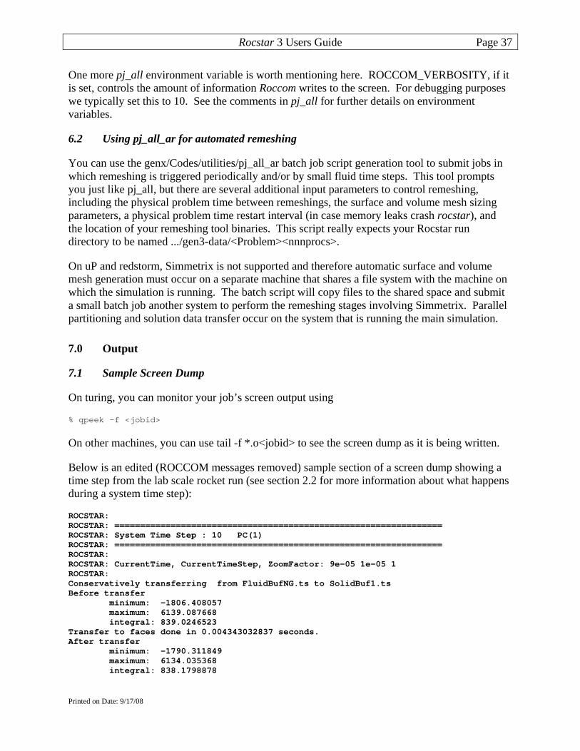
Rocstar 3 Users Guide Page 37
One more pj_all environment variable is worth mentioning here. ROCCOM_VERBOSITY, if it is set, controls the amount of information Roccom writes to the screen. For debugging purposes we typically set this to 10. See the comments in pj_all for further details on environment variables.
6.2 Using pj_all_ar for automated remeshing
You can use the genx/Codes/utilities/pj_all_ar batch job script generation tool to submit jobs in which remeshing is triggered periodically and/or by small fluid time steps. This tool prompts you just like pj_all, but there are several additional input parameters to control remeshing, including the physical problem time between remeshings, the surface and volume mesh sizing parameters, a physical problem time restart interval (in case memory leaks crash rocstar), and the location of your remeshing tool binaries. This script really expects your Rocstar run directory to be named .../gen3-data/<Problem><nnnprocs>.
On uP and redstorm, Simmetrix is not supported and therefore automatic surface and volume mesh generation must occur on a separate machine that shares a file system with the machine on which the simulation is running. The batch script will copy files to the shared space and submit a small batch job another system to perform the remeshing stages involving Simmetrix. Parallel partitioning and solution data transfer occur on the system that is running the main simulation.
7.0 Output
7.1 Sample Screen Dump
On turing, you can monitor your job’s screen output using
% qpeek –f <jobid>
On other machines, you can use tail -f *.o<jobid> to see the screen dump as it is being written.
Below is an edited (ROCCOM messages removed) sample section of a screen dump showing a time step from the lab scale rocket run (see section 2.2 for more information about what happens during a system time step):
ROCSTAR: ROCSTAR: ================================================================ ROCSTAR: System Time Step : 10 PC(1) ROCSTAR: ================================================================ ROCSTAR: ROCSTAR: CurrentTime, CurrentTimeStep, ZoomFactor: 9e-05 1e-05 1 ROCSTAR: Conservatively transferring from FluidBufNG.ts to SolidBuf1.ts Before transfer minimum: -1806.408057 maximum: 6139.087668 integral: 839.0246523 Transfer to faces done in 0.004343032837 seconds. After transfer minimum: -1790.311849 maximum: 6134.035368 integral: 838.1798878
Printed on Date: 9/17/08
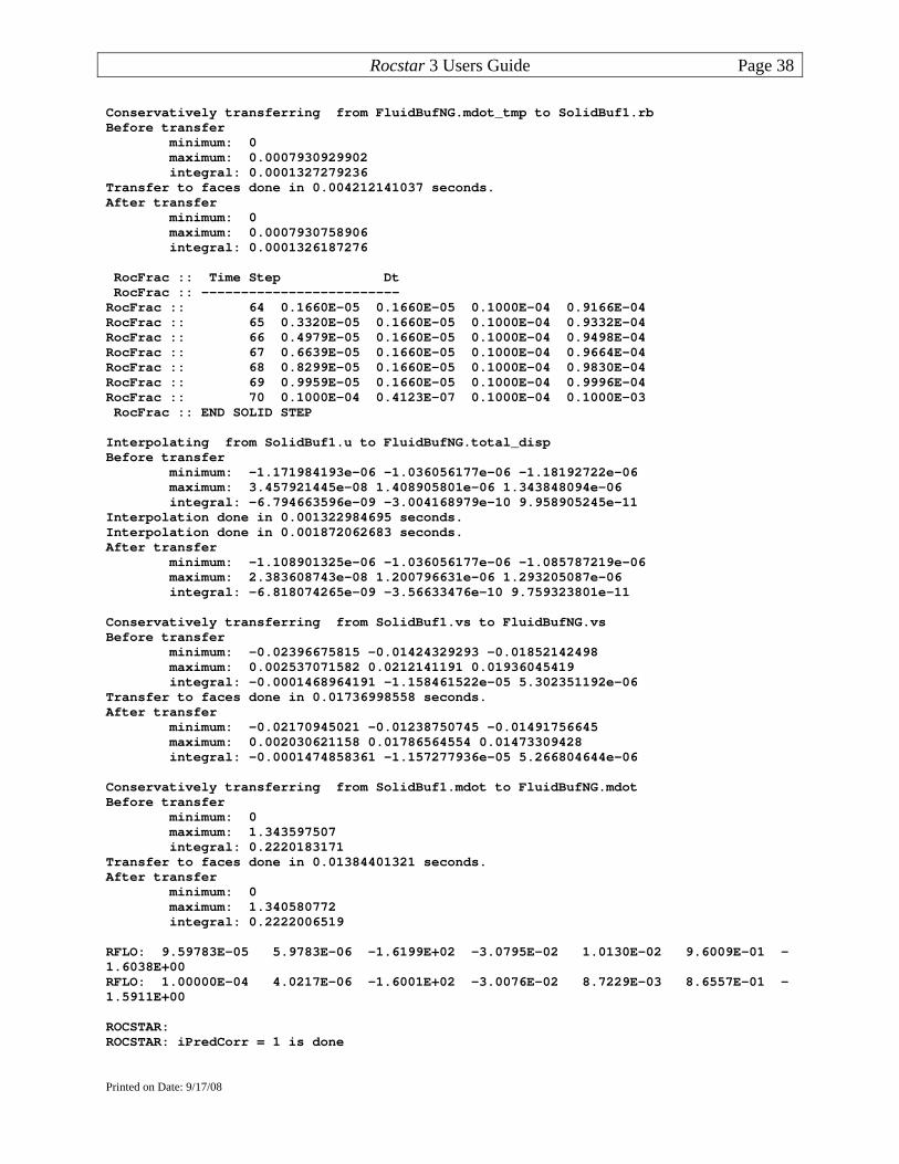
Rocstar 3 Users Guide Page 38
Conservatively transferring from FluidBufNG.mdot_tmp to SolidBuf1.rb Before transfer minimum: 0 maximum: 0.0007930929902 integral: 0.0001327279236 Transfer to faces done in 0.004212141037 seconds. After transfer minimum: 0 maximum: 0.0007930758906 integral: 0.0001326187276 RocFrac :: Time Step Dt RocFrac :: ------------------------- RocFrac :: 64 0.1660E-05 0.1660E-05 0.1000E-04 0.9166E-04 RocFrac :: 65 0.3320E-05 0.1660E-05 0.1000E-04 0.9332E-04 RocFrac :: 66 0.4979E-05 0.1660E-05 0.1000E-04 0.9498E-04 RocFrac :: 67 0.6639E-05 0.1660E-05 0.1000E-04 0.9664E-04 RocFrac :: 68 0.8299E-05 0.1660E-05 0.1000E-04 0.9830E-04 RocFrac :: 69 0.9959E-05 0.1660E-05 0.1000E-04 0.9996E-04 RocFrac :: 70 0.1000E-04 0.4123E-07 0.1000E-04 0.1000E-03 RocFrac :: END SOLID STEP Interpolating from SolidBuf1.u to FluidBufNG.total_disp Before transfer minimum: -1.171984193e-06 -1.036056177e-06 -1.18192722e-06 maximum: 3.457921445e-08 1.408905801e-06 1.343848094e-06 integral: -6.794663596e-09 -3.004168979e-10 9.958905245e-11 Interpolation done in 0.001322984695 seconds. Interpolation done in 0.001872062683 seconds. After transfer minimum: -1.108901325e-06 -1.036056177e-06 -1.085787219e-06 maximum: 2.383608743e-08 1.200796631e-06 1.293205087e-06 integral: -6.818074265e-09 -3.56633476e-10 9.759323801e-11 Conservatively transferring from SolidBuf1.vs to FluidBufNG.vs Before transfer minimum: -0.02396675815 -0.01424329293 -0.01852142498 maximum: 0.002537071582 0.0212141191 0.01936045419 integral: -0.0001468964191 -1.158461522e-05 5.302351192e-06 Transfer to faces done in 0.01736998558 seconds. After transfer minimum: -0.02170945021 -0.01238750745 -0.01491756645 maximum: 0.002030621158 0.01786564554 0.01473309428 integral: -0.0001474858361 -1.157277936e-05 5.266804644e-06 Conservatively transferring from SolidBuf1.mdot to FluidBufNG.mdot Before transfer minimum: 0 maximum: 1.343597507 integral: 0.2220183171 Transfer to faces done in 0.01384401321 seconds. After transfer minimum: 0 maximum: 1.340580772 integral: 0.2222006519 RFLO: 9.59783E-05 5.9783E-06 -1.6199E+02 -3.0795E-02 1.0130E-02 9.6009E-01 -1.6038E+00 RFLO: 1.00000E-04 4.0217E-06 -1.6001E+02 -3.0076E-02 8.7229E-03 8.6557E-01 -1.5911E+00 ROCSTAR: ROCSTAR: iPredCorr = 1 is done
Printed on Date: 9/17/08

Rocstar 3 Users Guide Page 39
ROCSTAR: Success: predictor-corrector converged at time 0.0001 Interpolating from SolidBuf1.nc to FluidBufNG.nc_tmp Before transfer minimum: 0.1523988448 -0.06096000224 -0.06098448113 maximum: 0.8503919693 0.06096000224 0.06098448113 integral: 0.085774316 6.985323444e-07 3.266980792e-07 Interpolation done in 0.001280069351 seconds. Interpolation done in 0.001846075058 seconds. After transfer minimum: 0.1523989079 -0.06096000224 -0.06087604562 maximum: 0.8503919693 0.06096000224 0.06087240779 integral: 0.08581958588 -6.335279164e-08 2.182600023e-07 ROCSTAR: Dumping restart files... done. ROCSTAR: ROCSTAR: ROCSTAR: ================================================================ ROCSTAR: System Time Step : 11 PC(1) ROCSTAR: ================================================================
The step begins by transferring the traction and burn rate computed at the end of the previous system time step from the fluid and combustion solvers to the solid solver. Next Rocfrac performs 7 internal time steps to reach the advanced time level. Then the new interface displacements, solid interface velocity, and mass injection rate are transferred to the fluids solver. Rocflo takes 2 internal time steps to reach the advanced time level, and the explicit coupled step is considered complete.
At the beginning of the screen dump, the batch job script writes out most of the text input files used by the run to show the parameter values for that particular simulation.
7.2 Performance Data
Rocstar automatically collects certain timing data; a sample is shown below (from RocstarProfile00.txt):
************** Solver times up to time step 9 since last output ********* Function #calls Time(tree) Time(self) ---------------------------------------------------------------------------- Rocflo.update_solution 1 0.805141 0.803968 Rocfrac.update_solution 1 0.368882 0.367827 RFC.least_squares_transfer 4 0.079227 0.079227 RFC.interpolate 1 0.0372121 0.0372121 PROP.propagate 1 0.00101995 0.00101995 BLAS.sub 54 0.000814676 0.000814676 SURF.compute_bounded_volumes 1 0.00067997 0.00067997 Fluid.obtain_bc 18 0.001086 0.000382185 MAP.reduce_maxabs_on_shared_node 1 0.000274181 0.000274181 BLAS.div_scalar 32 0.000254393 0.000254393 BLAS.limit1 25 0.000219822 0.000219822 BLAS.copy 16 0.000211 0.000211 BLAS.axpy_scalar 47 0.000200748 0.000200748 Solid.obtain_bc 7 0.00105524 0.000191212 BLAS.mul 11 0.000153065 0.000153065 SURF.compute_element_areas 1 6.60419e-05 6.60419e-05 BLAS.mul_scalar 2 6.19888e-05 6.19888e-05 BLAS.add 3 6.10352e-05 6.10352e-05 BLAS.neg 10 5.88894e-05 5.88894e-05
Printed on Date: 9/17/08

Rocstar 3 Users Guide Page 40
BLAS.copy_scalar 3 3.79086e-05 3.79086e-05 BLAS.axpy 9 3.71933e-05 3.71933e-05 BLAS.div 2 2.59876e-05 2.59876e-05 Fluid.obtain_gm 2 8.67844e-05 2.47955e-05 BLAS.sub_scalar 1 1.5974e-05 1.5974e-05 BLAS.maxof_scalar 1 1.40667e-05 1.40667e-05 Burn-Agent.obtain_bc 1 1.28746e-05 8.82149e-06 RocburnAPN.update_solution 1 2.38419e-05 7.86781e-06 RocburnAPN.update_internal 1 1.5974e-05 3.09944e-06 ---------------------------------------------------------------------------- Total(top level calls) 1.29306
The “self” column gives the timing exclusive of any children. Rocflo uses the most time, followed by Rocfrac, and then Rocface data transfer routines. The other functions do not use a significant amount of wall clock time.
7.2.1 Subroutine Level Profiling with Rocprof
Users of Rocstar may get subroutine and statement-level profiling using Rocprof. Rocprof is enabled at compile time with the addition of the ROCPROF=1 option to the (g)make command. At the completion of a successful Rocstar run, when MPI_Finalize is invoked, a summary of the root processor's (rank = 0) profile is generated and dumped to stdout. The profiles for the individual processors can be found in the Rocstar Run Directory. Profiles follow the naming convention: Rocstar.prof_<rank> A Rocstar configuration file is also created in the Rocstar Run Directory. This file maps internal integer IDs to the names supplied by the user in the instrumentation calls. The configuration file naming convention is: Rocstar.rpconfig. On platforms where hardware performance counters (HWC) are available, HWC data is also produced for single-processor runs. HWC data file formats vary from system to system, and we won't attempt to summarize it here. HWC data is generally written in human-readable text files with a section on each routine. These summaries are very useful for tuning single-processor performance, but much less so for parallel runs. Thus, we turn it off for non-serial runs. The profiles must be post-processed to produce summary information. The Rocprof post processor “profane” (in the Rocstar bin directory) can be invoked for one or all of the profiles produced during the run. Normally, for a parallel run, the user wishes to get a summary of the parallel performance and will want to process all of the profiles at the same time. One would do this with the following command: % ${ROCSTAR_HOME}/bin/profane -c Rocstar.rpconfig -o 2p_summary Rocstar.prof_* Profane generates a summary resembling the following: #Statistics for Rocflu (2 procs): #----------------------------------Inclusive Statistics------------------------------ # Min Inc Min Max Inc Max Mean Inc #Routine Name Duration Rank Duration Rank Duration Std Dev
Printed on Date: 9/17/08
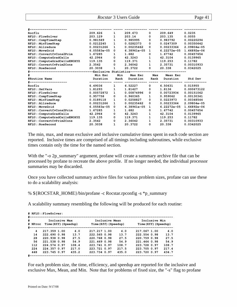
Rocstar 3 Users Guide Page 41
#-------------------- ------------ ----- ------------ ----- ------------ ------------ Rocflu 209.626 1 209.673 0 209.649 0.0235 RFLU::FlowSolver 203.129 1 203.14 0 203.135 0.0055 RFLU::CompTimeStep 0.981589 1 0.985995 0 0.983792 0.00220294 RFLU::MinTimeStep 0.0212245 1 0.0282373 0 0.0247309 0.00350642 RFLU::Allreduce 0.00231266 1 0.00235462 0 0.00233364 2.09804e-05 RFLU::MoveGrid 6.05583e-05 0 6.38961e-05 1 6.22272e-05 1.66892e-06 RFLU::ConvertCvCons2Prim 1.67285 1 1.682 0 1.67742 0.00457654 RFLU::ComputeGradCells 42.2964 0 42.3243 1 42.3104 0.0139965 RFLU::ComputeGradCellsENOXYZ 119.135 0 119.371 1 119.253 0.11782 RFLU::ConvertCvPrim2Cons 2.3542 0 2.36042 1 2.35731 0.00310933 RFLU::RoeSecond 20.3038 1 20.3722 0 20.338 0.0342025 #----------------------------------Exclusive Statistics------------------------------ # Min Exc Min Max Exc Max Mean Exc #Routine Name Duration Rank Duration Rank Duration Std Dev #-------------------- ------------ ----- ------------ ----- ------------ ------------ Rocflu 6.49036 1 6.52227 0 6.50631 0.015955 RFLU::SetVars 1.81293 1 1.81427 0 1.8136 0.000673122 RFLU::FlowSolver 0.00572872 1 0.00874996 0 0.00723934 0.00151062 RFLU::CompTimeStep 0.957758 0 0.960365 1 0.959062 0.00130341 RFLU::MinTimeStep 0.0189118 1 0.0258827 0 0.0223973 0.00348544 RFLU::Allreduce 0.00231266 1 0.00235462 0 0.00233364 2.09804e-05 RFLU::MoveGrid 6.05583e-05 0 6.38961e-05 1 6.22272e-05 1.66892e-06 RFLU::ConvertCvCons2Prim 1.67285 1 1.682 0 1.67742 0.00457654 RFLU::ComputeGradCells 42.2964 0 42.3243 1 42.3104 0.0139965 RFLU::ComputeGradCellsENOXYZ 119.135 0 119.371 1 119.253 0.11782 RFLU::ConvertCvPrim2Cons 2.3542 0 2.36042 1 2.35731 0.00310933 RFLU::RoeSecond 20.3038 1 20.3722 0 20.338 0.0342025
The min, max, and mean exclusive and inclusive cumulative times spent in each code section are reported. Inclusive times are comprised of all timings including subroutines, while exclusive times contain only the time for the named section. With the "-o 2p_summary" argument, profane will create a summary archive file that can be processed by profane to recreate the above profile. If no longer needed, the individual processor summaries may be discarded. Once you have collected summary archive files for various problem sizes, profane can use these to do a scalability analysis: % ${ROCSTAR_HOME}/bin/profane -c Rocstar.rpconfig -s *p_summary A scalability summary resembling the following will be produced for each routine: # RFLU::FlowSolver: #----------------------------------------------------------------------------- # Inclusive Max Inclusive Mean Inclusive Min # NProc Time(Eff)(Speedup) Time(Eff)(Speedup) Time(Eff)(Speedup) #----------------------------------------------------------------------------- 4 217.359 1.00 4.0 217.217 1.00 4.0 217.067 1.00 4.0 14 222.690 0.98 13.7 222.565 0.98 13.7 222.554 0.98 13.7 28 220.938 0.98 27.5 220.768 0.98 27.5 220.759 0.98 27.5 56 221.538 0.98 54.9 221.469 0.98 54.9 221.464 0.98 54.9 112 224.574 0.97 108.4 223.741 0.97 108.7 223.728 0.97 108.7 224 224.357 0.97 217.0 223.721 0.97 217.5 223.705 0.97 217.4 448 223.745 0.97 435.2 223.734 0.97 435.0 223.720 0.97 434.7 #----------------------------------------------------------------------------- For each problem size, the time, efficiency, and speedup are reported for the inclusive and exclusive Max, Mean, and Min. Note that for problems of fixed size, the "-s" flag to profane
Printed on Date: 9/17/08
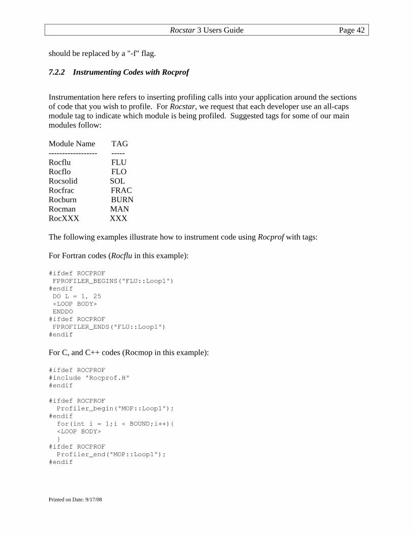
Rocstar 3 Users Guide Page 42
should be replaced by a "-f" flag. 7.2.2 Instrumenting Codes with Rocprof
Instrumentation here refers to inserting profiling calls into your application around the sections of code that you wish to profile. For Rocstar, we request that each developer use an all-caps module tag to indicate which module is being profiled. Suggested tags for some of our main modules follow: Module Name TAG ------------------ ----- Rocflu FLU Rocflo FLO Rocsolid SOL Rocfrac FRAC Rocburn BURN Rocman MAN RocXXX XXX The following examples illustrate how to instrument code using Rocprof with tags: For Fortran codes (Rocflu in this example): #ifdef ROCPROF FPROFILER_BEGINS("FLU::Loop1") #endif DO L = 1, 25 <LOOP BODY> ENDDO #ifdef ROCPROF FPROFILER_ENDS("FLU::Loop1") #endif For C, and C++ codes (Rocmop in this example): #ifdef ROCPROF #include "Rocprof.H" #endif #ifdef ROCPROF Profiler_begin("MOP::Loop1"); #endif for(int i = 1;i < BOUND;i++){ <LOOP BODY> } #ifdef ROCPROF Profiler_end("MOP::Loop1"); #endif
Printed on Date: 9/17/08

Rocstar 3 Users Guide Page 43
Code-construct names have a maximum length of 32 characters. Exceeding this limit does not break profiling, but it does make the profiling summary output uglier.
7.3 HDF Output Dumps and Probe Files
The .HDF output files will be located in the various Rocout directories. These files contain the numerical solution at a series of different physical problem time values. The fluids codes can also output text files called “probe files” that track the values of several variables at user-defined points within the grid. These files are placed in the Rocflo/Modout or Rocflu/Modout directories. The image below shows a plot of the head-end pressure vs. time for the explicit and implicit (“Dual Time Stepping”) schemes in Rocflo for the lab scale rocket:
The HDF files whose names include “00.000000” correspond to time t = 0, and are always written out for every simulation. The files whose names include strings such as “07.100000” correspond to later times. They can be interpreted as exponential notation, multiplied by 10-9. Thus, the files shown are for 0.1x107 x 10-9= 10-3 seconds. All Rocstar HDF output files use this convention so that an alphanumeric listing of the files is also in chronological order.
The fluid solver writes “fluid_nn.nnnnnn_*.hdf” files containing volumetric data (pressure, temperature, velocity, etc), and ifluid_b*.hdf files containing field variable solutions on the interacting surface grid (“b” stands for “burning”). Up to two more surface data file sets may
Printed on Date: 9/17/08

Rocstar 3 Users Guide Page 44
exist: ifluid_nb*.hdf files are at interacting but “non-burning” surfaces; while files named ifluid_ni*.hdf are at non-interacting non-burning surfaces. There may not be any non-interacting interfaces in a given problem. Finally, Rocout produces fluid_in_nn.nnnnnn.txt and ifluid_in_nn.nnnnnn.txt files, which tell Rocin the names of the variables that were written and how the blocks were distributed among the processors. These are used for restarting the run.
Rocstar HDF files may be visualized with the Rocketeer visualization package. See the on-line Rocketeer Users Guide (http://www.csar.uiuc.edu/F_software/rocketer), a tutorial.
Like the fluid HDF files, the solid*.hdf HDF files contain volumetric data, the isolid_b*.hdf files are solutions on the burning solid surface (interface with the fluids), the isolid_nb*.hdf files contain solutions on interacting but non-burning surfaces, and the isolid_ni*.hdf files contain solutions on non-interacting surfaces.
Rocketeer can visualize both the solid and fluid solutions at the same time. The figure below shows the 16-partition lab scale rocket results at 0.008 seconds. The yellow-red-black cylinder is the solid propellant (showing the displacement magnitude; scale on right hides the nozzle), and the fluid domain shows several temperature isosurfaces. The image is clipped at z = 0 to show the interior. The plume region is to the lower right.
The following image shows the partitions in different colors. This is achieved by making a surface plot of the “mesh” scalar variable.
Printed on Date: 9/17/08

Rocstar 3 Users Guide Page 45
Printed on Date: 9/17/08

Rocstar 3 Users Guide Page 46
The image above shows one mesh quality measure – the maximum dihedral angle between cell faces. It is close to 180 degrees in 4 columns of cells that run the length of the rocket. To improve the mesh quality, one should ideally produce a “circle-square” core block, as shown on the Truegrid web page (http://www.truegrid.com/pipe1.html). It is not as easy to produce this type of core block in Gridgen.
The image above shows a plot of the Courant time step in the fluid domain. It is smallest in cells along the walls of the nozzle because the cells are relatively small and the fluid velocity magnitude is relatively large here. Recall that the Courant limit is basically the local crossing time for the fastest signal, and is therefore proportional to the linear dimension of the cell (in the direction of the fastest signal). In the nozzle, the flow is supersonic, so the bulk speed of the fluid is the fastest signal speed.
There are sets of HDF files located in the Rocburn<version>/Rocout directories, but these files are used less frequently than the fluid and solid solution files. A few variables, such as the propellant surface temperature are available in those files (with the ignition model in RocburnPY) that are not in the other files. They may be visualized in Rocketeer like the other hdf files, but Rocketeer depends on being able to read the fluid results in the Rocflo/Rocout or Rocflu/Rocout directories to obtain the grid, since Rocburn does not write out the grid itself.
Printed on Date: 9/17/08

Rocstar 3 Users Guide Page 47
8.0 Examples and Test Problems
The following is a list of the test cases currently in the Native Data Archives by subject, grouped according to the type of model. Many of these problems have multiple grid and/or input parameter file sets. Problems marked with an * are available only to US citizens. Problems marked with ^ contain proprietary data, and will not be disseminated beyond CSAR without permission.
Real Rockets
• NASA Reusable Solid Rocket Motor (RSRM) *
The latest Rocflu unstructured mesh model has the submerged nozzle and correct inhibitor diameters in the joint slots. Our best mesh has some 4.5 million tetrahedra. Some mixed meshes also exist, but there are some regions of low resolution in the star grain which affect the accuracy considerably. A corresponding Rocfrac mesh also exists for solving coupled problems. The igniter is modeled as a time-dependent non-interacting fluid injection boundary. The igniter mass flux has a piecewise linear time history that is a reasonable match to the published data. We use RocburnPY to compute the ignition transient19.
Printed on Date: 9/17/08

Rocstar 3 Users Guide Page 48
• Titan IV booster (titan)
This model includes a plume region. It is used to study propellant slumping at the joint slot. The pressure history was published in an AIAA paper by Cheng, et al, 1994. Multiple Rocflu and Rocflo meshes exist for the fluid domain, and multiple Rocfrac and Rocsolid meshes exist for the solid domain. This problem is quite a challenge for our mesh motion schemes. For Rocflu, it requires remeshing.
Printed on Date: 9/17/08

Rocstar 3 Users Guide Page 49
• China Lake Motor 13 (labscale)
This is the classic lab scale rocket. Several mesh types and resolutions exist for both fluid solvers and both solid solvers.
• Ballistic Test and Evaluation Systems Motor (bates)
Printed on Date: 9/17/08

Rocstar 3 Users Guide Page 50
The BATES motors are used to study the effect of aluminum content on motor efficiency. These simulations include burning aluminum droplets and smoke20. Only the propellant formulation is restricted data, not the geometry. We have fake propellant parameters in a data set that can be used by anyone. Idealized problems21
• Cylindrical Rocket (cylinder) This problem can be run on a single processor. It has been used for convergence studies. An equilibrium solution is known if there is no regression.
Printed on Date: 9/17/08

Rocstar 3 Users Guide Page 51
Printed on Date: 9/17/08

Rocstar 3 Users Guide Page 52
• Superseismic Shock (Arienti)
The angle that the shock front in the fluid domain deviates from vertical is a function of the shock Mach number. This asymptotic solution is used for fluid/structure interaction verification. Multiple mesh resolutions exist for Rocflo and Rocfrac. Another problem along these lines is the “shock panel” problem, in which a shock wave travels down a square duct until it encounters a thin panel.
Printed on Date: 9/17/08

Rocstar 3 Users Guide Page 53
• RSRM section near joint slot (inhibitor)
This simulation is used to study the effect on the turbulent flow of the flexible inhibitor protruding into the fluid domain22. Only a relatively short cylindrical section of the booster is modeled. An inflow boundary condition does a reasonable job of mimicking the flow inside the full booster. It is derived from the velocity profile at the corresponding location in one of our earlier full RSRM simulations. Here the mesh is much finer so that we can include turbulence. The motion of the flapping inhibitor is very difficult to follow using our existing mesh smoothing scheme for structured meshes in Rocflo.
Printed on Date: 9/17/08

Rocstar 3 Users Guide Page 54
Special case/Test/Verification problems
• Mass conservation (spongebar)
There are several similar test cases involving pistons that are used for verification if the order of accuracy and for studying the stability of time stepping schemes.
Printed on Date: 9/17/08

Rocstar 3 Users Guide Page 55
• Star Grain Slice (StarSlice)
This problem is used for surface propagation and mesh improvement tests. Recently added to our test suite is Tstar, essentially the entire star grain region of the titan. This is used to test surface propagation. Additional problem sets are added frequently.
9.0 References 1Dick, W., Heath, T., Fiedler, R., and Brandyberry, M., “Advanced Simulation for Solid Propellant Rockets”, 41st
AIAA/ASME/SAE/ASEE Joint Propulsion Conference and Exhibit, AIAA-2005-3990, July 10-13, 2005. 2Jiao, X., Zheng, G., Lawlor, O. S., Alexander, P. J., Campbell, M. T., Heath, M. T., and Fiedler, R. A., “An Integration
Framework for Simulations of Solid Rocket Motors,” 41st AIAA/ASME/SAE/ASEE Joint Propulsion Conference and Exhibit, AIAA-2005-3991, July 10-13, 2005.
3Haselbacher, A., “A WENO Reconstruction Algorithm for Unstructured Grids Based on Explicit Stencil Construction”, 41st AIAA/ASME/SAE/ASEE Joint Propulsion Conference and Exhibit, AIAA 2005-0879, July 10-13, 2005.
4Blazek, J., “Flow Simulation in Solid Rocket Motors Using AdvancedCFD,” AIAA/ASME/SAE/ASEE Joint Propulsion Conference and Exhibit ,AIAA-2003-5111, 2003.
5Jameson, A., Schmidt, W., and Turkel, E., “Numerical Solutions of the Euler Equations by Finite Volume Methods Using Runge–Kutta Time-Stepping Schemes,” AIAA Paper 81-1259, 1981.
6Batten P., Clarke N., Lambert C., and Causon D.M., "On the Choice of Wavespeeds for the HLLC Riemann Solver", SIAM J. Sii. Stat. Comput., vol. 18, no. 6, 1996, pp. 1553-1570.
7Roe, P.L., “Approximate Riemann Solvers, Parameter Vectors, and Difference Schemes,” J. Computational Physics, vol. 43, 1981, pp. 357-372.
8Wasistho, B., and Moser, R. D., “Simulation Strategy of Turbulent Internal Flow in Solid Rocket Motor,” Journal of Propulsion and Power, vol. 21, no. 2, 2005, pp. 251-263.
9Najjar, F. M., Massa, L., Fiedler, R., Haselbacher, A., Wasistho, B., Balachandar, S., and Moser, R. D., “Effects of Droplet Loading and Sizes in Aluminized BATES Motors: A Multiphysics Computational Analysis,” 41st AIAA/ASME/SAE/ASEE Joint Propulsion Conference, AIAA 2005-3997, July 10—13, 2005.
10Ferry, J., and Balachandar, S., “Equilibrium Expansion for the Eulerian Velocity of Small Particles”, Powder Technology, vol. 125, 2002, pp. 131-139.
Printed on Date: 9/17/08

Rocstar 3 Users Guide Page 56
Printed on Date: 9/17/08
11Tang, K. C., and Brewster, M. Q., “Dynamic Combustion of AP Composite Propellants: Ignition Pressure Spike”, AIAA/ASME/SAE/ASEE Joint Propulsion Conference, AIAA 2001-4502, 2001.
12Massa, L., Jackson, T. L., and Buckmaster, J., “Using Heterogeneous Propellant Burning Simulations as Subgrid Components of Rocket Simulations”, AIAA Journal, vol. 42, no. 9, 2004, pp. 1889-1900.
13Namazifard, A., and Parsons, I. D., “A distributed memory parallel implementation of the multigrid method for solving three-dimensional implicit solid mechanics problems”, International Journal for Numerical Methods in Engineering, vol. 61, 2004, pp. 1173-1208.
14Brewer, M., Freitag, L., Knupp, P., Leurent, T., and Melander, D., "The Mesquite Mesh Quality Improvement Toolkit", Proceedings, 12th International Meshing Roundtable, Sandia National Laboratories, Sept. 2003, pp.239-250.
15Jiao, X., and Heath, M. T., “Common-Refinement Based Data Transfer Between Nonmatching Meshes in Multiphysics Simulations”, International Journal for Numerical Methods in Engineering, Vol. 61(14), 2004, pp. 2402-2427.
16Jaiman, R. K., Jiao, X. Geubelle, P. H., and Loth, E., “Assessment of Conservative LoadTransfer for Fluid-Solid Interface, with Nonmatching Meshes”, Int. J. Numer. Meth. Engng., Vol. 0, 2004, pp. 1-45.
17Lee, J., Winslett, M., Ma, X., and Yu, S., “Tuning High-Performance Scientific Codes: The Use of Performance Models to Control Resource Usage During Data Migration and I/O”, in Proceedings of the 15th ACM International Conference on Supercomputing, June 2001.
18Huang, C., Lawlor, O., and Kale, L, “Adaptive MPI”, in Proceedings of the 16th International Workshop on Languages and Compilers for Parallel Computing, College Station, TX, October 2003.
19Fiedler, R. A., Haselbacher, A., Breitenfeld, M. S., Alexander, P., Massa, L., and Ross, W. C., “3-D Simulations of Ignition Transients in the RSRM,” AIAA/ASME/SAE/ASEE Joint Propulsion Conference and Exhibit, AIAA-2005-3993, July 10-13, 2005.
20Najjar, F. M., Massa, L., Fiedler, R., Haselbacher, A., Wasistho, B., Balachandar, S., and Moser, R. D., “Effects of Droplet Loading and Sizes in Aluminized BATES Motors: A Multiphysics Computational Analysis,” 41st AIAA/ASME/SAE/ASEE Joint Propulsion Conference, AIAA 2005-3997, July 10-13, 2005
21Brandyberry, M., Fiedler, R., and McLay, C., “Verification and Validation of the Rocstar 3-D Multi-physics Solid Rocket Motor Simulation Program”, 41st AIAA/ASME/SAE/ASEE Joint Propulsion Conference, AIAA 2005-3992, July 10-13, 2005
22Wasistho, B., Fiedler, R., Namazifard, A., and Brandyberry, M., “3-D Coupled Simulations of Flexible Inhibitors in the RSRM,” 41st AIAA/ASME/SAE/ASEE Joint Propulsion Conference and Exhibit, AIAA-2005-3996, July 10-13, 2005
23Jiao, X., Face Offsetting: a Unified Framework for Explicit Moving Interfaces, Journal of Computational Physics, Vol. 220(2), pp. 612-625 (2006).
24Haselbacher, A., Najjar, F. M., Massa, L., and Moser, R., Enabling Three-Dimensional Unsteady SRM Burn-Out Computations by Slow-Time Acceleration, 42nd AIAA/ASME/SAE/ASEE Joint Propulsion Conference and Exhibit, AIAA-2006-4591 (Jul 2006).