rocket measurements of the equatorial airglow: multifot 92 database

~ ) Pergamon Journal of Atmospheric and Terrestrial Physics, Vol. 58, No. 16, pp. 1943-1961, 1996

Copyright © 1996 Elsevier Science Ltd Printed in Great Britain. All rights reserved

0021-9169(95)00158-1 0021-9169/96 SIS.00+0.00

Rocket measurements of the equatorial airglow: MULTIFOT 92 database

Hisao Takahashi, 1. B. R. Clemesha/D. M. Simonich, 1 Stella M. L. Melo, 1 N. R. Teixeira,' Agnaldo Eras /J . Stegman 2 and G. Witt 2

qnstituto Nacional de Pesquisas Espaciais, INPE C.P. 515, 12201/970, S~o Jos6 dos Campos, SP, Brasil;

2Meteorology Department, Stockholm University, S 10691, Stockholm, Sweden

(Received in final form 6 July 1995; accepted 7 July 1995)

Abstract--The MULTIFOT airglow photometer payload was launched from Alc~intara (2.5°S, 44.4°W) on a SONDA III rocket at 23:52 hrs local time on 31 May 1992. A total often photometers, six forward- looking and four side-looking, measured the height profiles of the airglow emissions 02 Herzberg band system, OI 557.7 nm, NaD 589.3 nm, OI 630.0 nm, OH(8,3) band R branch at 724.0 nm, 02 Atmospheric (0,0) band at 762.0 nm and the sky background at 578 nm and 710 nm. At the time of launch, a ground- based airglow photometer observed the intensity variations of these emissions, together with the rotational temperature of the OH(9,4) band, and a sodium lidar measured atomic sodium concentration from 80 to 110 km. Copyright © 1996 Elsevier Science Ltd

INTRODUCTION

A useful technique for studying the oxygen-hydrogen chemistry in the upper mesosphere and the lower thermosphere is tile study of oxygen-related airglow emissions, their vertical emission profiles, and their nocturnal and seasonal variations. Vertical profiles of the volume emission rates of the OI 557.7 nm airglow, the O2 Atmospheric (0,0) band at 761.9 nm, and the OH vibrational bands, for example, have been used to infer the atomic oxygen concentration between 80 and 110 km (McD,ade and Llewellyn, 1988; Gobbi et al., 1992).

Although there are still some uncertainties con- cerning the oxygen-related photochemistry, i.e. pro- duction, quenching and reaction rates, recent improvements in our understanding of the processes involved make it possible to infer the atomic oxygen concentration, for example, with reasonable accuracy (McDade et al., 1986a; Murtagh et al., 1990). However, our understanding is still incomplete, especially in the case of the reaction scheme and quenching proces,;es involved in the OH emissions (Rodrigo et al., 1989).

The latitudinal variation of the atomic oxygen pro-

* INPE, Cx Postal. 515, 12201-970 S~o Jos6 dos Campos, SP, Brazil. Fax: 55 123 25 6952. e-mail: INPEDAA@E- U.ANSP.BR.

file is not well known. It is expected that the atomic oxygen distribution should be strongly related to transport processes in the upper mesosphere. Dynami- cal processes such as eddy diffusion and internal grav- ity wave propagation are expected to be latitude dependent. Although many rocket experiments to investigate the airglow emissions have been carried out at middle and high latitudes (Greer et al., 1986), very little data is available from the equatorial and low latitude regions.

If sodium density can be measured simultaneously with the NaD airglow emission it is possible to determine the ozone concentration (Kirchhoff et al., 1981; Clemesha et al., 1993) and, with the aid of the OH emission intensity, it is then possible to estimate the hydrogen concentration (Takahashi et al., 1992). The operation of a sodium lidar near to the launch ramp during the MULTIFOT experiment made it possible to implement this technique. In view of the lack of ozone and hydrogen measurements at heights above 80 km, especially at night, the simultaneous measurement of airglow profiles by rocket and the Na profile by lidar forms a useful technique for measuring the vertical distributions of H and 03.

The purpose of the present paper is to present the vertical profiles of airglow emission obtained in the MULTIFOT experiment, together with the simultaneous ground-based airglow observations and the lidar measurements. The database constituted by

1943

1944 H. Takahashi et al.

these observations will be used in a number of sub- sequent photochemical studies.

THE MULTIFOT EXPERIMENT

The main purpose of the MULTIFOT experiment was to make a simultaneous measurement of the vertical profiles of a number of oxygen-related airglow emissions. In order to achieve this aim, the MUL- TIFOT payload contained six forward-looking and four side-looking photometers. In addition to the total of ten photometers, the payload included a pulsed plasma probe and an electron temperature probe. The payload configuration is shown in Fig. 1. The six forward-looking photometers were mounted in the first payload bay below the nose cone. In order to avoid heat conduction from the rocket body the complete six-photometer unit was thermally insulated from the rest of the payload structure. The four side- looking photometers were mounted in the second and third payload bays, and viewed the atmosphere through 2" diameter quartz windows inserted into the payload skin. In the case of the side-looking photometers thermal insulation was achieved by mounting the photometers, on bulkheads made from low-conductivity composite material.

The vehicle used for the MULTIFOT experiment was the SONDA III sounding rocket developed by the Brazilian Institute for Space and Aeronautics (IAE). This is a two stage vehicle with a 30 cm diam-

ELECTRON TEMPERATURE PULSED PLASMA PROBE PROBE I

eter second stage, having a capacity to carry a payload of approximately 100 kg to 600 km altitude. The present experiment used a shortened version of the SONDA III vehicle, which carried the 105 kg payload to an apogee of 282 km. The relevant flight parameters are listed in Table 1.

Payload photometers

The photometers used in the MULTIFOT payload are illustrated in Fig. 2. Both the forward-looking and side-looking photometers are conventional in design, with an interference filter to select the emission line, and a lens and diaphragm to determine the field of view (FOV). The forward-looking photometers also included a Fabry lens. In all photometers, the photo- multipliers (PMTs) are used in the photon counting mode, with Amptek 101 charge-sensitive preampli- fiers. Photometer signals were registered by 10-bit counters at a sample rate of 250 s -l , with each indi- vidual sample being telemetered to the tracking station.

The photometer characteristics are summarized in Table 2. Bi-alkali PMTs were used for photometers with wavelengths below 600 nm. At longer wavelengths $20 type PMTs were employed. The forward- looking photometers used a relatively wide FOV (8 ° full angle) to achieve maximum throughput with a limited wavelength resolution. Since the side-looking photometers see the airglow emissions integrated over a much longer quasi-horizontal path, it was possible to use a much smaller FOV. This smaller angular aperture is essential if good height resolution is to be achieved in the process of inverting the horizon brightness to derive the vertical emission profile.

ING (6)

(4)

Fig. 1. MULTIFOT payload configuration.

Table 1. Flight Data

Vehicle Site

Date Time

Elevation angle at launcher Apogee Horizontal range Nose cone opening height Spin rate Mean zenith angle Precession cone angle Precession period

SONDA III Alcfintara Launch Center (2.3 ° S, 44.4 ° W) 31 May 1992 23:52 Local Standard Time (02:52 UT on 1 June 1992) 82 ° 282 km 398 km 68 km 4s-t 26.2 ° 6.8 ° 14.7 s

Geophysical data for 31 May 1992 Ap 8 Y.Kp index 15 + F10.7 cm solar flux 101.8


FIELD LENS FILTER / DISC

SHU'I'I'E R/CALIBRATION

FABRY LENS PREAMP

CALIBRATION SOURCE

1945

(a) Fo r w ar d - l ook ing p h o t o m e t e r

FIELD LENS SHUTTER/CALIBRATION FILTER / D ISCo O PRE~P

SIGNAL I ~ \ o o o J

(b) S ide - look ing p h o t o m e t e r

Fig. 2. MULTIFOT photometers.

Table 2. MULTIFOT rocket photometer characteristics

Eraission 2o (nm) A2 (nm) PMT Sensitivity*

Forward-looking photometers (° 02 Herzberg I 275.0 14.3 EMI 9924Q 191.0 Ol 5577 557.7 1.7 EMI 9924 684.0 BG continuum at 578 nm 576.8 11.0 EMI 9924 220.2 NaD 589.0 1.7 EMI 9924 326.9 O1-1(8,3) 724.3 1.9 EMI 9798 143.9 O~A(0,0) 759.5 5.7 EMI 9798 43.6 Side-looking photometers (2) NaD 589.0 1.8 EMI 9924 84.1 OI 6300 629.9 1.6 EMI 9798 21.6 BG continuum at 713 nm 710.2 10.9 EMI 9798 - - O1:I(8,3) 724.3 1.8 EMI 9798 41.4

* Counts s- l Rayleigh-' (o 46 mm effective optical diameter; (2) 46 mm effective optical diameter;

with 2.4 ° FOV.

8 ° FOV 3.8 ° FOV, except for the OI 6300 photometer

The absolute sensitivities of the pho tomete r s were cal ibrated before l aunch using a MgO screen illumi- na ted by a l abora to ry sub-s tandard light source (Eppley ES 8315 cal ibra t ion lamp). A tiny t r i t ium

act ivated light source m o u n t e d on a ro ta t ing shut ter disc was used to provide a sensitivity check dur ing the flight. The ro ta t ing shut ter also made it possible to make an in-flight check of the photomul t ip l ie r da rk

1946

noise. Calibration of the 02 Herzberg photometer was carried out at Stockholm University using a calibrated deuterium lamp.

Multi-2 9round-based airglow photometer

The Multi-2 six channel multicolour tilting filter photometer constructed at INPE has the capacity to measure the zenith intensity of OI 557.7 nm, NaD 589 nm, OI 630.0 nm, OH(9,4) band Q(775.0 nm) and R (772.0 nm) branches and the O2 Atmospheric (0,1) band at 866.0 nm. In order to cover the large spectral region, from visible to near-infrared, a photo- multiplier with a GaAs cathode (Hamamatsu R943- 02) was used. A description of the photometer has been published elsewhere (Takahashi et al., 1989). The OH rotational temperatures are obtained from the intensity ratio between the R and Q branch intensities of the OH (9,4) band. Since the rotational temperature indicates the ambient atmospheric temperature in the emission layer, a simultaneous measurement of the temperature and the OH emission profile makes it possible to determine the height to which the temperature refers.

Na lidar

A major objective of the MULTIFOT experiment was the simultaneous determination of the vertical profiles of the NaD airglow emission and the Na density, an experiment which had never been carried out before. Measurements of the vertical profile of atmospheric sodium density were made using the transportable lidar system shown in Fig. 3, specifications of which are given in Table 3. The lidar includes a sodium vapour cell for calibration purposes, and is similar in principle (although not in its mechanical layout) to the S~o Jos6 lidar described by Simonich et al. (1979) and Clemesha (1984). The equipment was installed at the launch site, 5 km from the ramp, and was operated throughout the campaign.

H. Takahashi et al.

FLIGHT CONDITIONS

A SONDA III sounding rocket with the MUL- TIFOT payload was launched during a magnetically quiet period on 31 May 1992, at 23:52 h Local Stan- dard Time (1 June, at 02:52 UT). The start of the launch window was at 19:30 h, but the time of launch was delayed because of cloudy conditions over the launch area. The ground-based instruments operated from the beginning of the night. The frequent passage of cloud patches over the zenith made it difficult to determine the Na profile and airglow intensities reliably. Since the existence of adequate airglow inten-

Tx Rx

Fig. 3. PORTAL lidar configuration.

Table 3. PORTAL lidar specifications

Dye laser transmitter Receiver

Wavelength 589 nm Fresnel Lens 0.4 m 2 Bandwidth 6 pm Bandwidth 1 nm Pulse length 2 ps Ht. resolution 250 m Rep. Rate 1 pps Efficiency 1%

sities and sodium density was a prerequisite for the experiment it was only possible to launch after 23:00 h, when sky conditions improved, and it was possible to obtain the Na profile, airglow intensities and rotational temperature with reasonable precision.

The flight parameters are shown in Table 1. After second stage burnout, the rocket nose-cone opened at around 68 km altitude. At this point the payload spin axis was inclined at a mean angle of 26 ° to the vertical, and the spin rate was 4 s -~. The two-axis magnetometer indicated that no significant attitude change occurred after nose-cone ejection. The most important attitude information for the analysis of the forward-looking photometer signals is the zenith angle of their FOVs. Fortunately, it is possible to estimate the rocket axis zenith angle from the side- looking photometer output, as will be described later.

Rocket measurements of the equatorial airglow: MULTIFOT 92 database 1947

GROUND-BASED DATA

Na lidar

Sky conditions were unfavourable during most of the campaign, and most lidar data were obtained by firing through gaps in the cloud cover. For this reason the signal-to-noise ratio of the profiles obtained was poor when compared with typical results from modern lidars. On the other hand, on the night of the rocket experiment, adequate profiles were obtained both before and during 1:he launch. The average Na profile for a 50 minute period centred on the time of launch is shown in Fig. 4, and numerical data with error estimates are listed in Table 10. The very sharp cut- offs at around 82 km on the bottomside of the profile, and 98 km on the topside, are unusual. A more normal profile, also shown in Fig. 4, was observed on the day prior to the MULTIFOT launch. It was fortuitous that the profile measured at the time of the rocket experiment showed unusual and well defined features, allowing us to make a more useful comparison with the airglow profile,;.

Ground-based airglow photometer results

Ground-based airglow observation was started at 19:00 h. Owing to cloud patches frequently passing over the observing site, it was initially difficult to deter-

mine the airglow intensities reliably. After 23:00 h, sky conditions improved and continued good up to 01:00 h when observations were discontinued. The observed nocturnal variations of the airglow intensities and the rotational temperature are shown in Fig. 5. A lack of data between 22:00 h and 23:00 h in the OH(9,4) and NaD intensities is due to bad sky conditions. The oxygen green line and 02 Atmospheric (0,1) band intensities show a typical nocturnal variation, decreasing from evening to midnight, most probably controlled by a semi-diurnal tidal oscil- lation. Accurate measurements of the intensities and rotational temperature, listed in Table 4, were obtained around midnight during the launch.

ROCKET PHOTOMETER DATA

Determination of vehicle attitude

In order to derive emission profiles from the height variation of the integrated emission intensities, measured by the forward-looking photometers, it is necessary to know the zenith angle of the photometer FOV. Because of vehicle precession and the effects of aerodynamic drag, the zenith angle varies continu- ously. Consequently, it is necessary to determine its complete time history. This was achieved in the fol-

110

95

85

8 0

75

_ ~_ 920530

- ~ 920531

~v

' I ' I ' I ' I ' I '

0 . 0 0 . 5 1 . 0 1 . 5 2 . 0 2 . 5 3 . 0

c ¢nmaon (xl0 em Fig. 4. Na density profiles.

3.5


800

6O0

4O0

200

8O0

6OO

400

2OO

3OO

200

100

18

o o

OH(9,4) Oo ~ o (~0° ° ~ ° ( ~ ° °°

¢ o

NaD ¢ o

O A(0,t) 0

0

o o ° o

°dp ~d ~ Ooo o o

O1557.7 ~ .. ° ° ° o ~ C ~

T(OH)

0

o o ° o o oOO Oo 0 0 0 0

0 0

100

8O

4O

2O

0

I [ I I I I I

19 20 21 22 23 0 1 2 ur)

Fig. 5. Nocturnal variation of the airglow intensities and the OH rotational temperature observed at Alc~ntara on 31 May 1992.

lowing way. When the vehicle was well above the emission layers, payload spin, together with the 26 ° average zenith angle of the rocket axis, caused the FOVs of the side-looking photometers to view the emission region during only part of each rotation, for the remainder of the rotation they looked out into space. Knowing the height of the payload and the height of the emission layer, it is possible to determine the mean zenith angle for each rotation from the ratio between the time which the photometer spends looking down on the layer to that which it spends looking

out into space. This technique was implemented using data from the side-looking 724.0 nm photometer for several complete precession periods close to apogee. This process gave the mean zenith angle, the cone angle of precession and the period of precession. It was then assumed that these parameters did not change during the ballistic part of the flight. The magnetometer data is consistent with the data from the side-looking photometers. From magnetometer data alone, it is not possible to derive the vehicle attitude. Using the magnetometer and the photometer data


Table 4. Integrated airglow intensities and OH(9,4) band rotational temperature. The ground-based data were aver-

aged between 23:50 and 00:10 h

(;round- Rocket, Rocket, Emission* based upleg downleg

02 Hz I - - 133+2 147+2 OI 5577 124+3 123+4 135+_4 NaD 32+9 34+2 OH(9,4) 590+ 16 - - - - Toll (K) 189 _ 3 - - - - OH(8,3) - - - - 568_+ 37 O2A(0.0) - - - - 4500 4- 60 O2A(0,1) 282 + 6

*The units are Rayleigh except Toll (rotational temperature) in K.

together it is pos,dble to derive a complete determination of the time-history of the rocket axis vector (Clemesha and Takahashi, 1995).

To determine hew the zenith angle changed during the passage of the payload through the emission layers, where aerodynamic effects influence the vehicle attitude, the following procedure was adopted. When the payload was below the emission layer the side- looking photometers, at the highest point in their sweep, registered the integrated emission from the entire layer at an unknown zenith angle. As the vehicle passed through 1:he emission region this signal decreased to zero, and the signal seen at the lowest part of the sweep increased from zero, below the layer, to a maximum at the point when the entire layer had been penetrated, where it included the entire integrated emission from the layer. At any point, below, within or above tile layer, the sum of the signals at the lowest and highest points in the sweep should correspond to the integrated emission from the entire layer, viewed at a zenith angle that has to be determined. Provided the emission layer is spherically stratified it is easy to see that it is possible to determine the instantaneous zenith pointing angle by comparing this integrated intensity with that measured when the payload was above the layer, where its zenith angle had been determined by the procedure explained in the preceding paragraph.

Forward-looking p~otometers

The OI 557.7 nm, 02 Herzberg, BG 578 and NaD photometers functioned normally during both the upleg and downleg passage through the emitting region. Since local weather conditions at Alcantara are invariably hot, around 28°C at the time of launch, the noise level of the photometers using PMTs with $20 cathodes (type 9798 tubes) was relatively high.

1949

Temperature sensors in the payload showed that there was no increase in the photometer body temperatures during the flight. The 713 nm background photometer became very noisy shortly before the time of launch and saturated soon afterwards, making it impossible to use the data from this instrument to estimate the background for the OH (8,3) measurement.

During upleg, the 724.0 nm and 02 Atmospheric (0,0) band photometers suffered strong interference, starting before the nose-cone opened, and lasting throughout the passage of the payload through the emitting region. This noise disappeared completely about 50 s later, but it was impossible to reduce the upleg data from these two photometers. The wide band (10 nm) BG 578 nm photometer does not appear to have been affected by this interference, but does appear to have suffered a low level optical contamination. The level of this signal was around 5 Rayleighs nm- t, which is of the same order as the airglow continuum intensity. The 557.7 and 589.0 nm photometers appear to have suffered from the same contamination as the 578 nm instrument. Since the 557.7 and 589.0 photometers viewed the same atmospheric volume as the background instrument, it was possible to eliminate the contamination from these photometers by subtracting a suitable fraction of the 578 nm signal, before differentiating to obtain the emission profile. In doing this we have assumed that the spectrum of the contamination is fiat between 557.7 and 589.0 nm. Any error resulting from this assumption should be small, since the subtracted background is much smaller than the airglow signal. The fact that the upleg profiles differ little from those obtained during downleg, where no contamination was observed, helps to validate this procedure. Even in the absence of contamination, the signal-to-noise ratio of the 578 nm photometer was such as to make it impossible to obtain a useful emission profile for the continuum.

No strong light contamination, such as the vehicle glow seen in one of our earlier rocket experiments (Clemesha et al., 1987), was detected in the present experiment. This could be the result of both the con- siderably lower velocity of the shortened SONDA III used in the present experiment, and the different payload configuration.

The observed integrated intensities for each photometer, interpolated at 0.5 km intervals, are listed in Table 5 and Table 6 together with the photometer zenith angles. The data in these tables were converted to Rayleighs using the nominal photometer sensitivities. The astronomical background has been subtracted but the data have not been corrected for airglow continuum, neither have they been corrected


Table 5. Integrated intensities, in Rayleighs, of the 557.7, 275 and 589 nm emissions (forward-looking photometers)

Altitude 557.7 nm 557.7 nm 275 nm 275 nm 589 nm 589 nm (km) Upleg Downleg Upleg Downleg Upleg Downleg

81.0 138.5 198.8 32.7 52.6 72.0 90.6 81.5 139.9 192.9 31.6 52.2 75.1 90.1 82.0 142.5 186.3 32.0 44.6 76.6 87.4 82.5 141.3 180.4 30.8 39.9 73.1 83.3 83.0 142.7 176.4 30.4 41.0 73.6 78.7 83.5 141.9 171.8 31.5 36.9 72.1 74.8 84.0 141.1 169.6 30.3 36.9 69.3 72.4 84.5 143.5 166.3 30.7 34.9 68.2 68.0 85.0 145.5 161.3 30.4 34.9 66.0 66.9 85.5 145.3 159.5 27.9 33.6 61.9 62.0 86.0 147.2 157.4 31.1 31.8 63.3 54.9 86.5 149.1 154.8 31.2 32.3 62.9 55.7 87.0 149.3 156.7 28.9 29.5 59.4 46.4 87.5 156.0 153.7 34.0 28.1 63.7 42.8 88.0 156.2 149.2 33. I 27.2 62.7 41.1 88.5 160.7 148.2 34.7 27.6 63.5 39.5 89.0 164.8 148.4 33.2 23.4 62.8 36.0 89.5 164.4 148.1 34.0 25.2 61.6 34.1 90.0 164.6 147.0 34.7 27.1 61.1 31.9 90.5 164.8 145.5 34.8 25.0 59.4 31.4 91.0 163.7 147.2 35.1 28.2 57.5 29.2 91.5 159.7 147.4 35.8 28.6 54.6 28.7 92.0 157.8 146.7 30.7 25.9 51.6 26.5 92.5 154.6 146.4 33.2 28.8 45.8 27.5 93.0 149.4 144.0 32.0 25.7 44.4 22.0 93.5 148.4 143.5 30.0 26.1 39.4 21.8 94.0 144.3 142.5 28.0 25.7 37.4 20.2 94.5 142.0 138.9 26.5 26.7 35.8 18.6 95.0 135.8 139.2 26.7 26.1 31.0 18.0 95.5 132.5 137.9 26.0 24.5 29.5 16.0 96.0 129.6 131.3 25.3 25.0 28.3 12.4 96.5 125.9 128.9 23.0 23.9 24.9 9.0 97.0 121.1 120.5 22.8 20.2 23.5 7.1 97.5 114.4 114.9 23.3 21.3 20.2 5.6 98.0 108.7 107.9 20.5 18.5 16.8 3.6 98.5 104.0 95.9 18.8 16.6 16.9 2.8 99.0 94.6 85.5 17.4 15.6 15.4 0.8 99.5 85.4 74.8 17.6 12.9 14.4 1.2

100.0 75.6 64.4 17.0 13.4 15.8 1.0 100.5 65.6 56.4 14.1 10.9 17.9 1.5 101.0 56.4 49.2 12.3 11.5 12.8 0.3 101.5 46.1 41.9 8.7 8.1 11.2 2.2 102.0 38.7 34.8 6.5 8.6 9.9 2.4 102.5 32.5 30.1 5.8 7.3 7.8 1.9 103.0 26.1 24.5 4.7 8.3 7.9 3.5 103.5 20.8 19.5 4.0 6.0 7.8 0.9 104.0 16.3 16.3 4.2 3.5 8.4 0.8 104.5 13.4 11.3 3.6 2.4 5.8 1.6 105.0 12.3 9.3 4.1 2.8 4.7 0.5 105.5 10.3 5.8 5.3 1.7 4.6 0.4 106.0 9.8 4.8 4.1 3.1 5.5 1.9 106.5 8.7 2.6 2.3 1.9 6.0 0.1 107.0 7.7 1.8 3.3 1.2 4.4 0.0 107.5 7.2 2.5 1.4 1.0 4.4 0.2 108.0 5.1 2.4 1.6 0.5 3.2 0.6 108.5 4.7 2.4 0.5 0.2 3.4 0.0 109.0 4.0 2.7 1.3 1.3 2.9 2.0 109.5 2.9 1.2 0.8 0.6 0.8 0.3 110.0 2.8 1.3 0.6 1.7 2.5 0.7


Table 6. Integrated intensities, in Rayleighs, of the 578 nm, 759.5 nm and 724.3 nm emissions and photometer zenith angles (forward-looking photometers)

Altitude E;G 578 nm BG 578 nm 759.5 nm 724.3 nm Z. Angle Z. Angle (km) Upleg Downleg Downleg Downleg Upleg Downleg

80.0 70.5 31.5 7433 1086 21.0 51.5 80.5 72.2 33.9 6945 971 21.3 50.1 81.0 75.6 47.5 6687 920 21.9 48.9 81.5 79.4 51.2 6447 846 22.4 47.3 82.0 79.7 58.2 6279 835 23.1 45.1 82.5 75.1 49.5 6043 787 23.9 43.6 83.0 74.7 51.6 5942 753 24.5 42.0 83.5 62.1 53.6 5781 711 25.0 40.2 84.0 54.8 58.2 5690 676 25.3 38.7 84.5 56.5 48.6 5621 615 26.0 36.8 85.0 53.3 45.4 5524 573 27.0 35.2 85.5 45.5 36.5 5408 553 27.7 34.3 86.0 46.5 27.0 5326 511 29.0 33.1 86.5 40.0 25.7 5267 465 30.3 32.2 87.0 61.4 18.3 5077 427 31.5 31.1 87.5 67.7 10.5 4986 377 33.4 29.9 88.0 79.6 5.1 4906 353 35.1 29.0 88.5 88.2 2.8 4815 305 36.6 28.4 89.0 107.0 0.0 4676 260 37.6 27.8 89.5 110.0 0.0 4595 257 37.9 27.3 90.0 112.7 0.0 4453 246 38.1 26.9 90.5 118.5 3.5 4347 253 38.3 26.5 91.0 119.3 6.3 4189 186 38.0 26.0 91.5 123.0 11.6 4044 189 37.4 25.6 92.0 118.2 11.9 3922 168 36.8 25.3 92.5 107.8 9.3 3812 119 36.2 25.0 93.0 101.9 9.1 3654 109 35.5 24.7 93.5 103.8 5.1 3448 136 34.7 24.5 94.0 95.5 7.1 3420 78 34.1 24.3 94.5 87.7 7.0 3167 102 33.5 24.0 95.0 79.8 6.1 3018 62 32.7 23.8 95.5 77.9 6.4 2889 128 32.0 23.6 96.0 84.7 7.7 2753 79 31.3 23.4 96.5 81.5 10.9 2516 73 30.6 23.3 97.0 79.2 7.2 2278 28 29.8 23.3 97.5 80.2 10.6 2072 64 28.7 23.3 98.0 75.6 5.7 1849 44 27.8 23.3 98.5 78.1 2.7 1550 33 26.7 23.5 99.0 81.2 0.8 1398 0 25.8 24.0 99.5 83.0 0.3 1162 47 24.8 24.7

100.0 78.3 0.7 1016 19 23.7 25.7 100.5 78.3 0.8 865 54 22.9 26.5 101.0 68.6 5.6 716 21 22.0 27.2 101.5 63.0 7.8 600 44 21.1 27.9 102.0 50.5 11.0 563 42 20.5 28.6 102.5 47.8 8.5 401 13 20.0 29.2 103.0 39.7 15.4 341 33 19.7 29.9 103.5 39.1 8.7 260 8.1 19.5 30.6 104.0 38.7 6.3 191 45 19.4 31.3 104.5 33.9 3.9 160 1 19.4 32.0 105.0 34.7 2.6 106 11 19.5 32.1 105.5 32.5 0.4 122 20 19.7 32.5 106.0 29.6 0.0 60 33 20.0 32.0 106.5 31.6 0.0 54 0 20.3 31.5 107.0 30.3 0.0 50 20 20.8 30.9 107.5 22.4 0.0 40 7 21.3 30.3 108.0 21.5 3.0 51 0.0 21.9 29.6 108.5 17.1 6.3 24 7 22.6 28.9 109.0 14.6 2.6 30 14 23.3 28.1 109.5 9.9 3.8 15 29 24.1 27.3 110.0 6.6 0.9 40 13 24.9 26.5


for the van Rijn effect. It should be noted that the volume emission profiles presented later in this paper were obtained by doing the background subtraction and van Rijn correction on the original 4 ms data samples, without prior averaging. As explained below, smoothing of the profiles was carried out during the differentiation process used to obtain the emission profile.

Ol 557.7 nm, 02 Herzber9 and 02 atmospheric (0,0) bands. An incremental straight line fitting method (Murtagh et al., 1984) was used to derive the volume emission rate profiles. The technique was applied to 400 point data samples, corresponding to a fitting length of 3 km. The volume emission profiles of the OI 557.7 nm emission for both upleg and downleg are shown in Fig. 6. The upleg profile shows a peak at 100 km with a half-width of about 6 km. The peak of the downleg profile is slightly lower, at 99 km, with a half width of about 7 km. It should be noted that the downleg profile showed slightly higher intensity than that for the upleg below the peak, between 95 and 100 km. The volume emission rates and their estimated errors are listed in Table 7. The errors shown correspond to the standard error of the estimate in the linear regression analysis used to derive the emission profiles from the measured integrated intensities.

The 02 Herzberg photometer filter was centred at 275 nm with a bandwidth of 14.3 nm. The measured profiles are shown in Fig. 7. It should be noted that, as all the 02 excited states responsible for the ultraviolet nightglow emissions have strongly non-thermal vibrational population distributions, they produce a multitude of overlapping vibrational progressions dis- persed throughout the entire ultraviolet spectral region (Slanger and Huestis, 1981). For this reason, the profiles in Fig. 7 include contributions from both the 02 Herzberg I, 02 Herzberg II and 02 Chamberlain systems. In order to interpret the profiles of Fig. 7 in terms of the 02 Herzberg I total system emission, it is necessary to assume ratios for the relative intensities of the 02 Herzberg I, Herzberg II and Chamberlain bands, as well as a vibrational population distribution for the emitting states. An analysis of the results for the Herzberg I system will be presented in Melo et al. (1996).

The volume emission profile for the 02 Atmospheric (0,0) band, with a peak at 98 km and a half-width of about 11 km, is shown in Fig. 8 and Table 8.

NaD. In order to determine the intensity of the NaD (DI + D2) emission it is necessary to take into account spectral contamination from the OH(8,2) Q branch and the airglow continuum within the filter pass band.

120

115

110

~ , 105

95

i v

90

85 I ' I ' I ' I 0 50 100 150 200

Voltn~e ~ o n Rate ~ c m ' 3 . s "1)

Fig. 6. OI 5577 nm volume emission rate profiles.

Rocket measurements of the equatorial airglow: M U L T I F O T 92 database

Table 7. Volume emission rates of the OI 557.7 nm and 02 Herzberg band system in photons cm-3 s -

1953

Altitude 01555.7 Error 01557.7 Error 02 Hz Error 02 Hz Error (km) Upleg Downleg Upleg Downleg

85.0 . . . . 5.4 2.2 6.0 5.6 85.5 . . . . 3.5 2.5 9.3 6.0 86.0 3.9 4.0 - 17.4 4.0 0.7 2.8 12.8 5.7 86.5 19.0 3.9 - 16.6 4.0 - 1.1 3.0 16.4 5.1 87.0 26.1 3.8 -11 .1 4.0 - 2 . 1 3.1 19.2 4.8 87.5 26.6 3.8 - 5.7 4.0 - 1.8 3.2 20.5 4.5 88.0 21.0 3.7 - 4 . 3 4.0 - 1.3 3.3 18.8 5.7 88.5 15.5 3.7 - 3.2 4.0 - 1.3 3.4 13.6 7.6 89.0 9.7 3.6 - 2.4 4.0 - 1.1 3.3 6.1 7.4 89.5 5.7 3.6 - 1.5 4.0 0.1 3.3 - 2 . 0 6.7 90.0 5.7 3.7 - 0 . 1 4.0 1.6 3.3 - 11.3 6.4 90.5 6.5 3.7 1.5 4.0 2.2 3.1 - 14.8 6.3 91.0 5.8 3.7 - 1.7 4.0 3.0 2.8 - 9 . 8 6.8 91.5 6.5 3.6 - 3 . 5 3.9 5.8 2.8 - 3 . 0 7.4 92.0 10.0 3.7 2.7 4.0 9.0 2.8 3.0 6.8 92.5 13.7 3.9 9.5 4.0 10.9 2.8 7.2 5.9 93.0 17.3 3.9 14.6 4.0 12.8 2.8 6.4 5.7 93.5 20.8 3.9 19.5 4.0 14.9 2.7 4.4 5.6 94.0 26.2 3.9 21.9 4.1 17.0 2.5 3.7 3.7 94.5 33,2 3.9 24.8 4.2 15.5 2.3 3.7 1.9 95.0 41.3 3.8 35.0 4.3 13.0 2.2 8.3 2.8 95.5 49.4 3.7 52.9 4.3 12.5 2.3 15.6 4.1 96.0 52.2 3.6 74.1 4.2 12.7 2.4 16.0 4.7 96.5 54.1 3.5 95.2 4.1 13.2 2.2 18.2 5.3 97.0 60.2 3.5 116.3 4.0 14.0 2.0 23.1 5.8 97.5 72.7 3.4 137.4 3.9 15.1 2.0 28.1 6.2 98.0 90.9 3.4 156.6 3.8 16.3 2.1 33.0 5.0 98.5 109.6 3.4 173.2 3.8 17.2 2.1 37.5 3.3 99.0 128.6 3.4 184.5 3.6 18.9 2.1 33.9 3.4 99.5 147.5 3.3 184.2 3.5 22.4 2.2 24.3 3.7

100.0 160.9 3.3 175.1 3.3 26.4 2.4 22.8 3.8 100.5 161.5 3.2 162.2 3.2 30.3 2.4 20.8 3.8 101.0 152.9 3.1 147.2 2.9 34.2 2.3 17.3 3.8 101.5 141.5 3.1 132.4 2.6 35.2 2.4 15.1 3.9 102.0 128.8 2.9 118.2 2.5 30,7 2.5 15.9 3.8 102.5 116.0 2.8 104.0 2.4 23,9 2.5 17.3 3.6 103.0 103.1 2.7 90.0 2.4 17,0 2.4 18.1 3.4 103.5 89.7 2.7 76.2 2.3 10,4 2.0 18.3 3.2 104.0 71.0 2.6 63.1 2.2 4.3 1.6 16.7 3.0 104.5 50.7 2.6 50.8 2.1 2,1 1.8 13.9 3.0 105.0 35.5 2.5 39.4 2.0 3,0 2.0 9.7 3.9 105.5 25.4 2.3 29.7 2.0 4,1 1.9 6.0 4.7 106.0 20.3 2.2 21.7 1.9 5,7 1.9 7.7 4.9 106.5 17.2 2.1 16.6 1.9 8,5 1.8 10.6 5.0 107.0 15.3 2.1 13.4 1.9 10.9 1.8 8.5 5.1 107.5 13.8 2.0 10.9 2.0 10.0 1.8 4.9 5.0 108.0 13.9 2.0 8.9 2.0 8.2 1.9 - 0 . 7 4.8 108.5 13.9 1.9 6.9 2.0 8.5 1.8 - 5 . 0 4.5 109.0 8.5 1.9 4.5 2.0 8.5 1.6 - 1.6 4.3 109.5 3.2 1.9 2.1 1.9 5.3 1.6 4.5 4.0 110.0 2.4 1.9 2.1 1.9 1.8 1.7 6.1 4.3

T h e c o n t r i b u t i o n o f the OH(8 ,2 ) w a s ca l cu l a t ed u s i n g

t he o b s e r v e d OH(8 ,3 ) b a n d i n t ens i t y w i t h a n a p p r o -

p r i a te i n s t r u m e n t a l f a c t o r a n d the ra t io o f the r e l e v a n t

t r a n s i t i o n p robab i l i t i e s . T h e c o n t i n u u m c o n t r i b u t i o n

in t he 589 n m r eg ion was e s t i m a t e d by u s i n g a n a p p r o -

p r i a te f r a c t i on o f t he c o n t i n u u m in t ens i t y o b s e r v e d a t

578 n m . F o r the up leg , in the a b s e n c e o f d a t a f r o m the

f o r w a r d - l o o k i n g 724.0 n m p h o t o m e t e r , t he OH(8 ,3 )

b a n d profi le de r ived f r o m the s i de - l ook ing p h o t o -

m e t e r was u s e d to e s t i m a t e t he OH(8 ,2 ) c o n t a m i -


120

115

110

95

9O

85

t Upl

- e - - Downleg

8 0 ' I ' I ' I ' I ' I ' I '

-20 -10 0 10 20 30 40 50

Volume F_mi~'on Rate (l~io~ls.cr~3.s "1) Fig. 7. Observed 02 Herzberg band system volume emission rate profiles.

110

105

100

9O

85

0 IOO0 2OO0 3OOO 40O0

Vohm~ ~ o n Rate ~ . c z n "3 .S "l) Fig. 8.02 Atmospheric (0,0) band volume emission rate profile (downleg).

Rocket measurements of the equatorial airglow: M U L T I F O T 92 database 1955

Table 8. Volume emission rates of the NaD, OH(8,3) and 02 Atmospheric (0,0) bands, in photons cm-3s -~

Altitude NaD Error NaD Error OH(8-3) Error O2A(0-0) Error (km) Upleg Downleg Downleg Downleg

83.0 4.4 3.6 17.7 2.7 288 37 - - - - 83.5 12.2 3.6 14.9 2.7 347 41 - - - - 84.0 19.4 3.6 12.2 2.7 404 43 - - - - 84.5 26.0 3.6 11.2 2.8 462 39 - - - - 85.0 31.8 3.6 12.5 2.8 499 35 95 120 85.5 37.7 3.6 16.4 2.8 498 36 436 125 86.0 41.4 3.6 20.5 2.8 490 39 578 114 86.5 41.2 3.5 24.3 2.7 492 43 709 101 87.0 42.1 3.5 27.8 2.7 492 47 817 106 87.5 46.1 3.4 24.4 2.7 486 45 953 111 88.0 46.8 3.4 19.2 2.7 473 42 1173 114 88.5 41.5 3.4 19.0 2.5 447 46 1417 113 89.0 37.8 3.4 19.3 2.4 424 49 1644 94 89.5 36.1 3.3 20.2 2.4 416 48 1837 71 90.0 35.0 3.2 20.8 2.4 408 46 1953 68 90.5 34.7 3.3 20.5 2.4 405 40 2045 64 91.0 35.0 3.3 20.2 2.3 391 35 2139 60 91.5 37.6 3.2 20.1 2.3 350 38 2230 56 92.0 37.9 3.1 20.2 2.2 300 43 2314 63 92.5 33.9 3.1 21.2 2.2 255 38 2396 75 93.0 32.0 3.1 22.7 2.2 210 35 2485 78 93.5 33.6 3.0 22.1 2.2 178 36 2575 81 94.0 35.1 2.9 22.0 2.2 166 37 2619 87 94.5 36.5 2.8 25.8 2.1 178 37 2666 95 95.0 38.3 2.8 30.3 2.1 191 37 2844 108 95.5 41.1 2.8 33.5 2.0 183 36 3124 116 96.0 42.9 2.8 35.8 1.9 170 35 3474 106 96.5 43.7 2.7 35.7 1.9 180 34 3834 93 97.0 43.6 2.6 31.8 1.9 192 33 4074 82 97.5 45.8 2.5 24.4 1.9 150 33 4196 72 98.0 40.9 2.6 16.9 1.8 89 33 4207 80 98.5 22.8 2.8 10.9 1.8 83 37 4060 97 99.0 9.7 2.9 7.0 1.8 80 41 3775 98 99.5 1.5 2.8 5.8 1.8 49 41 3442 97

100.0 - 2 . 1 2.7 4.8 1.8 20 40 3060 109 100.5 0.9 2.7 3.0 1.8 28 39 2681 122 101.0 4.1 2.7 1.3 1.8 41 39 2349 99 101.5 9.5 2.8 2.4 1.8 35 38 2065 69 102.0 11.0 2.8 3.9 1.8 28 38 1847 64 102.5 5.3 2.7 2.2 1.8 25 36 1636 63 103.0 2.1 2.6 0.4 1.8 23 33 1374 67 103.5 2.5 2.6 1.2 1.8 30 32 1109 69 104.0 3.1 2.6 2.0 1.8 38 31 855 58 104.5 4.9 2.6 0.1 1.7 26 31 648 45 105.0 4.8 2.5 - - - - 11 31 543 40 105.5 1.3 2.5 - - - - 15 30 456 37 106.0 . . . . 20 29 329 41 106.5 . . . . 5 28 208 45 107.0 . . . . . . 9.6 27 124 37 107.5 - - - - - - 11 27 88 31 108.0 . . . . 29 28 75 33 108.5 . . . . 11 29 70 36 109.0 . . . . . . 71 41

n a t i o n . F o r t he d.ownleg, a su i t ab le f r a c t i on o f t he 724.0 n m p h o t o m e t e r s igna l w a s s u b t r a c t e d f r o m the

589.0 n m s igna l direct ly . T h e N a D v o l u m e e m i s s i o n

prof i les o b t a i n e d in th is w a y for u p l e g a n d d o w n l e g

are p l o t t e d in Fig. 9 a n d l is ted in T a b l e 8. T h e s e

prof i les s h o w a d o u b l e p e a k e d s t r u c t u r e , w i th one


110

105

lOO

9O

85

80

Upleg

- - -G - D o w n l e g

q" ® s

0 10 20 30 40 50

Volume Emission Rate (photons.em3.s "~) Fig. 9. NaD volume emission rate profiles.

60

peak at 87 km and the other at 96 km, with a total layer width of about 12 km. The double peaked structure was also seen in the lidar profile of free sodium.

OH(8,3). In the case of the OH(8,3) R branch, spectral contamination at 724 nm from the airglow continuum was estimated from the continuum observed in the 578 nm region. In order to estimate the ratio between the intensities in the 724 nm and 578 nm regions we used data from the ETON campaign, presented by McDade et al. (1986b), leading to the adop- tion of a value of 1.33 for 1(724)/1(578 ). This ratio could, however, be height dependent. According to McDade and his coworkers, the ratio varies from 1.0 to 2.0 between 90 and 100 km. Nevertheless, the error due to this uncertainty should be negligible in the present study. The contribution of the continuum to the 724.0 nm photometer was around 8% of the total output. The uncertainty originating from the continuum subtraction, therefore, should be less than 3%, which is less than the experimental error. The resulting OH(8,3) emission profile is shown in Fig. 10 and Table 8. The peak height is around 87 km with a half-width of approximately 10 km. The observed integrated intensity, 568 Rayleighs (R), is somewhat larger than expected, on the basis of the OH(9,4) band intensity of about 590 R, measured by the ground-based photometer at the launch site.

Side-looking photometers

The side-looking photometers were included in the MULTIFOT payload because previous photometric experiments, using the SONDA III vehicle, had suffered from strong contamination effects at heights below 87 km. In view of the fact that these con- taminating signals appear to have been produced in the shock wave in front of the payload (Clemesha et al., 1987, 1988) it was reasoned that side-looking instruments should be much less sensitive to this sort of contamination. It is not clear whether or not this reasoning was justified because, as mentioned above, the contamination seen in the forward-looking photometer signals in the MULTIFOT experiment was very low and different in nature to that seen in previous experiments using the SONDA III vehicle. On the other hand, none of the side-looking photometers showed contamination signals.

In order to determine the intensity of the NaD emission it is necessary to take into account the airglow continuum and the OH(8,2) band emissions within the pass band of the photometer. Unfor- tunately, the 713 nm side-looking photometer included to measure the background signal failed to operate and, for this reason, we were unable to derive profiles for the NaD emission from the side-looking photometer. In the case of the 724 nm photometer,


110 ~

1957

105

100

9O

85

0 100 200 300 4(30 500 600

Volmm F_mission Rate (photons.caTl'3.s "1) Fig. 10. OH(8,3) volume emission rate profile from the forward-looking photometer (downleg).

the OH(8,3) band emission is much stronger, and the background subtraction is much less critical.

At the time of launch, the OI 630.0 nm emission intensity was very weak, the ground-based photometer indic~,ting an intensity of less than 5 Rayleighs. As a result of this it was not possible to obtain a profile for the F-region emission. The horizon intensities observecl by the 630.0 nm photometer are listed in Table 9. On the assumption that the variation of the horizon intensity between 70 and 120 km cor- responds to the continuum emission, the data in this region were used to estimate its intensity, and used to correct the OH(8,3) band profile derived from the 724.2 nm side-looking photometer.

To determine the OH(8,3) band intensity from the 724.2 nm side-looking photometer signals we applied an onion-skin type inversion process to the observed horizon intensity profile (horizon intensity, in this con- text, refers to the intensity seen by the photometer when its viewing angle is horizontal). The 2 ° FOV of the photometer was taken into account by decon- volving the inverted profile with an appropriate instrument function. The rocket payload rotated about its axis at 4 r.p.s., and the spin axis was inclined at a mean angle of 26 ° to the vertical, so the photometer FOV traversed the emitting layer eight times per second.

The horizon intensities were obtained by assuming that instants of maximum intensity correspond to the same vertical viewing angle for both the ascending and descending sweeps of the FOV through the emitting region. Averaging the times of maximum signal gives the instants of maximum and minimum inclination of the photometer FOV, and averaging these latter times gives the instants of horizon crossing.

The payload telemetry system sampled each photometer at 4 ms intervals, so that there were approximately 63 samples for each photometer per rotation of the payload. A simple three-point parabolic fit was used to determine the instants of maximum intensity and the horizon intensities. In the region of 90 km, the vertical component of the vehicle velocity was close to 1800 m s- 1, so the eight horizon crossings per second for each photometer correspond to 4.4 horizon intensity determinations per km of height. The raw data were smoothed by ten-point running means, before interpolating at 1 km intervals, giving an effective height resolution of slightly more than 2 km. In order to maximize the signal-to-noise ratio, no attempt was made to analyse opposite horizons separately.

The observed OH(8,3) horizon intensities, as a function of height for both upleg and downleg passage

1958 H. Takahashi e t al.

Table 9. 724.3 nm and 630 nm horizon intensities, in Rayleighs, observed by the side-looking photometers

Altitude 724.3 nm 724.3 nm 630 nm (km) Upleg Downleg Upleg

70.0 1019 966 122.7 71.0 1036 1005 125.0 72.0 1040 1018 106.5 73.0 1072 1003 89.1 74.0 1069 1008 99.5 75.0 1100 1064 111.1 76.0 1152 1094 126.2 77.0 1218 1095 119.2 78.0 1254 1107 134.3 79.0 1332 1157 152.8 80.0 1396 1256 159.7 81.0 1451 1357 179.4 82.0 1590 1501 187.5 83.0 1800 1655 219.9 84.0 2017 1823 245.4 85.0 2122 1904 255.8 86.0 2084 1990 263.9 87.0 2030 2028 263.9 88.0 2011 2006 262.7 89.0 1981 1858 251.2 90.0 1896 1708 233.8 91.0 1789 1599 233.8 92.0 1652 1393 229.2 93.0 1538 1232 203.7 94.0 1394 1094 179.4 95.0 1143 964 155.1 96.0 988 896 160.9 97.0 860 803 144.7 98.0 711 691 125.0 99.0 593 585 126.2

100.0 550 426 108.8 101.0 453 320 105.3 102.0 321 332 81.0 103.0 267 384 76.4 104.0 226 370 64.8 105.0 174 328 45.1 106.0 147 255 48.6 107.0 121 176 13.9 108.0 100 112 9.3 109.0 69 51 1.2 110.0 75 20 11.6

through the emission layer, are shown in Table 9 and Fig. 11, and the inverted profiles are shown in Table 10 and Fig. 12. Note that Fig. 12 shows the total OH(8,3) band intensity, determined by dividing the observed intensities by 0.216, which is the fraction of the OH(8,3) band that falls within the filter bandpass. As can be seen from these figures, there are only minor differences between the profiles, lending confidence to the assumption that they are free from contamination effects. The continuum correction applied to the signal from the side-looking 724 nm photometer was obtained from the 630 nm photometer by assuming

that the F-region OI 630 nm emission signal seen by this instrument was constant over the height range of the OH(8,3) emission. The final error involved in making this assumption, and in converting from 630 nm to 724 nm, should not be more than a few percent, since the total contribution of the continuum was only about 8% and, as mentioned earlier, the intensity of the F-region 630.0 nm emission was extremely low. The total band intensities measured for the upleg and downleg respectively were 397 R and 370 R. These values are smaller than that observed by the forward- looking photometer, which was 568 Rayleighs. The difference occurs mainly below about 92 km. It should be remembered, of course, that the side-looking photometers integrate over a horizontal path of several hundred km, whereas the forward-looking photometer measures an almost vertical profile, so that a close agreement with the profile derived from the latter instrument should not be expected.

Despite the difference in the regions of atmosphere viewed by the two instruments, the large difference in the OH(8,3) emission profiles observed by the forward-looking and side-looking photometers, together with the consistency between the upleg and downleg profiles from the side-looking instrument, suggests that we should look for possible sources of error in the profile from the forward-looking photometer. Below a height of 100 km on the downleg, aerodynamic drag started to cause large perturbations in payload attitude. These perturbations do not affect the measurement by the side-looking photometer, because the signal used is always that which refers to the point when the instrument views the horizon horizontally. The instants in time when this occurs are easy to determine with good precision. The signal from the forward-looking photometer must be corrected for the van Rijn effect, and to do this it is necessary to know the zenith angle of the photometer FOV at all times. The technique used for determining the time history of the vehicle attitude during the flight has been described. It was not possible to obtain consistent results from this technique at heights below 82 km, when the vehicle started to tumble. If the zenith angle was underestimated between this height and 90 km, above which height the profiles from the two instruments start to agree fairly well, then the intensity determined from the forward-looking instrument would have been insufficiently corrected for the van Rijn effect, resulting in the emission intensity being overestimated. Against this possibility is the fact that the NaD emission measured below 90 km on the downleg, using the same van Rijn correction, was actually weaker than that for the same region on the upleg. It may also be relevant that an analysis of the


120 -~

1959

1 1 0

lOO

80

0

- oH(8,3) Upleg

----o - OH(S,3) Downleg

/

I I t I I

500 1000 1500 2000 2500

Horizon immsities (Rayleigh) Fig. 11. OH(8,3) horizon intensities as a function of height observed by the side-looking photometer. The

continuum emission estimated from the OI 6300 photometer is also shown.

115

110

lO6

10o

95

90

85

80

-4-- OH(8,3) Up~g

- - e - - oI-~8,3)~wnleg

. . . . o~s,3) ~

I

0 100 200 300 400 500 600

Voltmav Emission Rate ~ c m 3 . s q) Fig. 12. OH(8,3) volume emission rate profiles observed by the side-looking photometer. The downleg

profile obtained from the forward-looking photometer is also shown for reference.


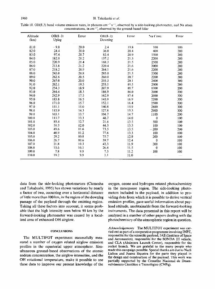
Table 10. OH(8,3) band volume emission rates, in photons c m -3 s - l , observed by a side-looking photometer, and Na atom concentrations, in c m -3 , observed by the ground-based lidar

Altitude OH(8-3) Error OH(8 3) Error Na Conc. Error (km) Upleg Downleg

81.0 -9 .8 20.0 2.4 19.8 100 100 82.0 24.4 20.0 36.0 20.4 400 200 83.0 97.4 20.7 83.4 20.9 1500 200 84.0 182.0 21.2 137.2 21.3 2200 200 85.0 220.9 21.4 168.3 21.5 2500 200 86.0 213.8 21.2 220.4 21.6 2000 200 87.0 218.2 20.9 264.1 21.6 2200 200 88.0 243.0 20.8 285.0 21.3 2300 200 89.0 262.6 20.5 260.0 20.7 2200 200 90.0 265.0 20.0 255.3 20.1 2400 300 91.0 262.1 19.5 253.1 19.5 2000 200 92.0 254.3 18.9 207.9 18.7 1300 200 93.0 264.4 18.3 186.9 18.0 2000 200 94.0 242.9 17.5 162.9 17.4 2000 300 95.0 183.8 16.5 145.9 16.9 2200 300 96.0 171.0 15.7 152.1 16.4 2500 300 97.0 151.1 15.0 140.8 15.9 2800 300 98.0 115.9 14.3 127.8 15.3 2900 300 99.0 103.1 13.7 104.7 14.7 1100 200

100.0 113.7 13.3 48.7 14.0 0 100 101.0 85.4 12.7 21.6 13.5 500 100 102.0 51.3 12.0 44.3 13.5 100 100 103.0 49.6 11.6 73.5 13.5 - 200 200 104.0 40.9 11.2 77.6 13.3 100 100 105.0 29.2 10.8 75.7 12.9 200 100 106.0 26.7 10.6 59.7 12.4 0 100 107.0 21.8 10.3 42.3 11.9 - 200 100 108.0 15.6 10.1 26.4 11.5 0 100 109.0 7.8 9.9 7.3 11.2 - 100 100 I10.0 19.2 9.9 1.1 11.0 - - - -

da ta f rom the side-looking photometers (Clemesha and Takahashi , 1995) has shown var ia t ions by nearly a factor of two, occurr ing over a hor izonta l distance of little more than 100 km, in the region of the downleg passage of the payload th rough the emit t ing region. Taking all these factors into account, it seems prob- able tha t the high intensi ty seen below 90 km by the forward- looking pho tomete r was caused by a local- ized area of enhanced O H airglow.

CONCLUSIONS

The M U L T I F O T exper iment successfully measured a n u m b e r of oxygen related airglow emission profiles in the equator ia l upper a tmosphere. Sim- ul taneous ground-based observat ions of the a tomic sodium concentra t ion , the airglow intensities, and the O H rota t ional temperature, make it possible to use these data to improve our present knowledge of the

oxygen, ozone and hydrogen related photochemis t ry in the mesopause region. The side-looking photometers included in the payload, in addi t ion to pro- viding da ta f rom which it is possible to derive vertical emission profiles, gave useful in fo rmat ion abou t payload att i tude, unob ta inab le f rom the forward- looking instruments . The da ta presented in this repor t will be analysed in a n u m b e r of o ther papers dealing with the photochemis t ry of the a tmospher ic region in question.

Acknowledgements--The MULTIFOT experiment was carried out as part of a cooperative programme involving INPE, responsible for the scientific payload, IAE (Institute of Space and Aeronautics), responsible for the SONDA III vehicle, and CLA (Alcfintara Launch Center), responsible for the rocket launch. We are grateful to the many people who made this campaign possible. Special thanks are due to Narli Lisboa and Juarez Siqueira for the parts they played in the design and construction of the payload. This work was partially supported by the Conselho Nacional de Desen- volvimento Cientifico e Tecnol6gico (CNPq).


Clemesha B. R.

Clemesha B. R., Takahashi H. and Sahai Y.

Clemesha B. R, Takahashi H. and Sahai Y.

Clemesha B. R. and Takahashi H.

Clemesha B. R., Simonich D. M., Takahashi H. and Melo S. M. L.

Gobbi D., Takahashi H., Clemesha B. R. and Batista P. P.

Greer R. G. H., Murtagh D. P., McDade I. C., Dickinson P. H. G., Thomas L., Jenkins D. B., Stegman J., Llewe],lyn E. J., Witt G., Mackinnon D. J. and Williams E. R.

Kirchhoff V. W. J. HI., Clemesha B. R. and Simonich D. M.

McDade I. C., Murtagh D. P., Greer R. G. H., Dickinson P. H. G., Witt G., Stegman J., Llewellyn E. J., Thomas L. and Jenkins D. B.

McDade I. C., LleweUyn E. J., Greer R. G. H. and Murtagh D. P.

McDade I. C. and L]ewellyn E. J.

Melo S. M. L., Takahashi H., Clemesha B. R. and Stegman J.

Murtagh D. P., Greer R. G. H., McDade I. C., Llewellyn E. J. and Bantle M.

Murtagh D. P., Witt G., Stegman J., McDade I. C., Llewellyn E. J., Harris F. and Greer R. G. H.

Rodrigo R., Lopes-Moreno J. J., Lopes-Gonzalez M. J. and Garcia-Alvarez E.

Simonich D. M., Clemesha B. R. and Kirchhoff V. W. J. H.

Slanger, T. G. and Huestis, D. L.

Takahashi H., Sahai Y., Clemesha B. R., Simonich D. M., Teixeira N. R., Lobo R. M. and Eras A.

Takahashi H., Clemesha B. R., Sahai Y., Batista P. P. and Simonich D. M.

REFERENCES

1984 Lidar studies of the alkali metals. Middle Atmosphere Handbook 13, 99.

1987 Vehicle glow observed during a rocket sounding experiment. Planet. Space Sci. 35, 1367.

1988 Contamination glow observed during two rocket sounding experiments. Progress in Atmospheric Physics, Kluwer Academic Publishers: 109.

1995 Rocket-borne measurements of horizontal structure in the OH(8,3) and NaD airglow emissions. Adv. Space Res. 17, 81.

1993 A simultaneous measurement of the vertical profiles of sodium nightglow and atomic sodium density in the upper atmosphere. Geophys. Res. Lett. 20, 1347.

1992 Equatorial atomic oxygen profiles derived from rocket observations of OI 557.7 nm airglow emission. Planet. Space Sci. 40, 775.

1986 Eton h A data base pertinent to the study of energy transfer in the oxygen nightglow. Planet. Space Sci. 34, 771.

1981 Seasonal variation of ozone in the mesosphere. J. yeophys. Res. 86, 1463.

1986a ETON 2: quenching parameters for the proposed pre- cursors of O2(blEg ÷) and O(1S) 557.7 nm in the terrestrial nightglow. Planet. Space Sci. 34, 789.

1986b Altitude profiles of the nightglow continuum at green and near infrared wavelengths. Planet. Space Sci. 34, 801.

1988 Mesospheric oxygen atom densities inferred from night-time OH Meinel band emission rates. Planet. Space Sci. 36, 897.

1996 The 02 Herzberg I bands in the equatorial nightglow. J. atmos, terr. Phys. (submitted).

1984 Representative volume emission profiles from rocket photometer data. Ann. Geophys. 2, 467.

1990 An assessment of proposed O(IS) and O2(b~Y,~ +) nightglow excitation parameters. Planet. Space Sci. 38, 43.

1989 Atomic oxygen concentrations from OH and 02 nightglow measurements. Planet. Space Sci. 37, 49.

1979 The mesospheric sodium layer at 23°S: nocturnal and seasonal variations. J. geophys. Res. 84, 1543.

1981 O2(c~,, + - -X3~g -) emission in the terrestrial nightglow. J. geophys. Res. 86, 3551.

1989 Equatorial mesospheric and F-region airglow emissions observed from latitude 4°S. Planet. Space Sci. 37, 649.

1992 Seasonal variations of mesospheric hydrogen and ozone concentrations derived from ground-based airglow and lidar observations. J. yeophys. Res. 97, 5987.

rocket measurements of the equatorial airglow: multifot 92 database

Documents