Electronic copy available at: http://ssrn.com/abstract=1341305Electronic copy available at: http://ssrn.com/abstract=1341305

Rock Center for Corporate GovernanceWoRkinG PaPeR SeRieS

Crown Quadrangle • 559 Nathan Abbott Way • Stanford, CA 94305rockcenter@law.stanford.edu • http://rockcenter.stanford.edu

Have Changes in Financial Reporting Attributes Impaired Informativeness? Evidence from the Ability of Financial Ratios to Predict Bankruptcy Rock Center Working Paper No. 13 Authors: William H. Beaver, Maria Correia and Maureen F. McNichols, Stanford Graduate School of Business School

Electronic copy available at: http://ssrn.com/abstract=1341305Electronic copy available at: http://ssrn.com/abstract=1341305

Have Changes in Financial Reporting Attributes Impaired Informativeness?

Evidence from the Ability of Financial Ratios to Predict Bankruptcy

William H. Beaver

fbeaver@stanford.edu

Maria Correia

mcorreia@stanford.edu

Maureen F. McNichols

fmcnich@leland.stanford.edu

Graduate School of Business

Stanford University

Stanford, CA 94305

First draft: August 2008

Current draft: December 9, 2008

Comments welcome

Electronic copy available at: http://ssrn.com/abstract=1341305Electronic copy available at: http://ssrn.com/abstract=1341305

Have Changes in Financial Reporting Attributes Impaired Informativeness?

Evidence from the Ability of Financial Ratios to Predict Bankruptcy

Abstract: This study explores the effect of cross- sectional and time-series differences in

financial reporting attributes on the predictive ability of financial ratios for bankruptcy.

We identify proxies for discretion over financial reporting, the importance of intangible

assets, and the effects of changing accounting standards over time. Our proxies include

earnings restatements, discretionary accruals, research and development intensity, book-

to-market ratios and incurrence of losses. We test the ability of financial ratios to predict

bankruptcy for a sample of bankrupt and non-bankrupt firms listed on NYSE/AMEX or

NASDAQ during the 1962-2002 period. Each of our proxies is associated with less

informative financial ratios as reflected in predictive ability for bankruptcy. We compare

the findings for the accounting model to those of a model based on market-related

variables, and find that the market-related variables do not compensate for the lessened

predictive ability of financial ratios. In our time-series analysis, descriptive statistics

confirm that each of our proxies exhibits a trend consistent with decreasing

informativeness over time. Our time-series tests reveal a decline in the predictive ability

of financial ratios for bankruptcy, and document that this decline is associated with our

financial reporting variables.

Keywords: bankruptcy, accounting information, financial ratios.

Data availability: For data availability, contact sources identified in the paper.

1

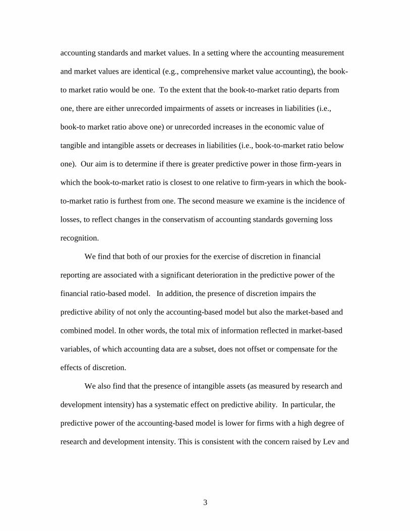
1. Introduction

A significant body of research has examined the ability of financial statement data

to predict bankruptcy. Beaver, McNichols and Rhie (2005), hereafter BMR, examine

whether there have been changes from 1962 to 2002 in the ability of financial ratios to

predict bankruptcy. In particular, BMR hypothesize that predictive ability has

deteriorated over time as a result of three forces: alleged increases in the frequency and

magnitude of discretion exercised in financial statements, increases in the magnitude of

intangible assets, and changes in the extent to which accounting standards capture

business fundamentals. The basic form of their analysis is to divide the forty-year time

period into two major sub periods, 1962-1993 and 1994-2002.

The key finding of BMR is that the predictive ability of financial ratios is

remarkably robust over time, showing only a slight deterioration. BMR also find that the

predictive ability of market-based variables shows a slight improvement over time, while

the combined model shows no deterioration in predictive power. This finding is

consistent with little, if any, net effect of the three forces discussed above on predictive

ability over time. An important qualifier is that BMR test for the net effect of these three

factors, as well as the possible effect of any other unidentified factors.

In this study, we expand the scope of BMR in two important ways. First, we

examine the effect of each of the three forces on the predictive ability of financial

statements for bankruptcy. Specifically, we conduct a cross-sectional analysis, which

allows us a more powerful test of differences in the predictive ability of bankruptcy

models. Moreover, it allows us to return to the original time series analysis informed by

what we have learned about the three forces from the cross-sectional analysis.

2

Specifically, we assess the predictive ability of financial ratios over time, and assess

whether it is associated with variation in our proxies for financial reporting attributes.

Second, we add NASDAQ firms to the sample, which more than doubles the

number of bankrupt firms in our study. Among other differences, the probability of

bankruptcy is approximately 1.4 times greater for NASDAQ firms relative to

NYSE/AMEX firms, which comprised the sample in the earlier study. An overriding

research design question in any study is the power of the test, particularly when there is a

failure to reject the null hypothesis of no difference or change. Our earlier time series

research design implicitly assumed that the time series variation in predictive ability was

of sufficient magnitude to be detected given other features of the research design. A

design alternative, the alternative taken in this paper, is to examine the effect of the three

forces on predictive ability in a cross-section. This can be a potentially more powerful

design to the extent that cross-sectional differences in the factors of interest are large

relative to differences over time.

To conduct our cross-sectional and time-series tests, we identify proxies for

discretion over financial reporting, the importance of intangible assets, and the effects of

changing accounting standards over time. To study the effects of discretion on predictive

power, we examine two measures—restatements of financial statements and measures of

discretionary accruals. To study the effect of unrecognized intangible assets, we examine

research and development intensity.

To study the effects of changes in accounting standards over time, we examine

two measures. The first is the book-to market ratio, which reflects the effects of

conservatism and intangible assets, as well as other measurement differences between

3

accounting standards and market values. In a setting where the accounting measurement

and market values are identical (e.g., comprehensive market value accounting), the book-

to market ratio would be one. To the extent that the book-to-market ratio departs from

one, there are either unrecorded impairments of assets or increases in liabilities (i.e.,

book-to market ratio above one) or unrecorded increases in the economic value of

tangible and intangible assets or decreases in liabilities (i.e., book-to-market ratio below

one). Our aim is to determine if there is greater predictive power in those firm-years in

which the book-to-market ratio is closest to one relative to firm-years in which the book-

to-market ratio is furthest from one. The second measure we examine is the incidence of

losses, to reflect changes in the conservatism of accounting standards governing loss

recognition.

We find that both of our proxies for the exercise of discretion in financial

reporting are associated with a significant deterioration in the predictive power of the

financial ratio-based model. In addition, the presence of discretion impairs the

predictive ability of not only the accounting-based model but also the market-based and

combined model. In other words, the total mix of information reflected in market-based

variables, of which accounting data are a subset, does not offset or compensate for the

effects of discretion.

We also find that the presence of intangible assets (as measured by research and

development intensity) has a systematic effect on predictive ability. In particular, the

predictive power of the accounting-based model is lower for firms with a high degree of

research and development intensity. This is consistent with the concern raised by Lev and

4

Zarowin (1999) that extant accounting for intangibles results in less informative financial

statements.

We find that predictive power of the bankruptcy model varies across book-to-

market classes in ways that suggest its effect is nonlinear. Specifically, those firm-years

with low to medium positive book-to-market ratios are most informative, consistent with

more informative financial statement results when the book value of equity is closer to

the market value of equity. Those firm-years with high book-to-market ratios are next

most informative, and the financial ratios of firms with negative book-to-market ratios

are least informative. In other words, when financial statements fail to recognize changes

in asset or liability values or intangible assets, the predictive ability of financial ratios is

impaired.

Furthermore, we find that the incidence of a loss significantly increases the

conditional probability of bankruptcy. However, we also find that the predictive power of

the bankruptcy model for loss firm-years is lower than for non-loss firm-years because of

a deterioration in the incremental explanatory power of the remaining variables.

Finally, we conduct time-series tests to assess whether the effects of financial

reporting attributes on predictive ability in the cross-section have implications for the

predictive ability of financial ratios for bankruptcy over time. We find that there is a

significant time trend in the frequency of restatements, larger magnitudes of discretionary

accruals, greater R&D intensity, book-to-market ratios that are further from one, and

losses. In addition, we find that these variables are individually significant in explaining

differences in predictive ability over time. Because these variables are highly correlated

with one other, however, it is difficult to isolate individual, incremental effects.

5

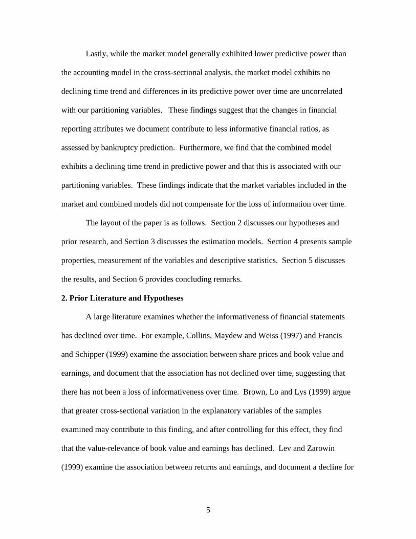
Lastly, while the market model generally exhibited lower predictive power than

the accounting model in the cross-sectional analysis, the market model exhibits no

declining time trend and differences in its predictive power over time are uncorrelated

with our partitioning variables. These findings suggest that the changes in financial

reporting attributes we document contribute to less informative financial ratios, as

assessed by bankruptcy prediction. Furthermore, we find that the combined model

exhibits a declining time trend in predictive power and that this is associated with our

partitioning variables. These findings indicate that the market variables included in the

market and combined models did not compensate for the loss of information over time.

The layout of the paper is as follows. Section 2 discusses our hypotheses and

prior research, and Section 3 discusses the estimation models. Section 4 presents sample

properties, measurement of the variables and descriptive statistics. Section 5 discusses

the results, and Section 6 provides concluding remarks.

2. Prior Literature and Hypotheses

A large literature examines whether the informativeness of financial statements

has declined over time. For example, Collins, Maydew and Weiss (1997) and Francis

and Schipper (1999) examine the association between share prices and book value and

earnings, and document that the association has not declined over time, suggesting that

there has not been a loss of informativeness over time. Brown, Lo and Lys (1999) argue

that greater cross-sectional variation in the explanatory variables of the samples

examined may contribute to this finding, and after controlling for this effect, they find

that the value-relevance of book value and earnings has declined. Lev and Zarowin

(1999) examine the association between returns and earnings, and document a decline for

6

both comprehensive and constant samples. Landsman and Maydew (2002) examine the

market reaction to earnings announcements over time, and find an increase in abnormal

price and volume reactions, consistent with an increase rather than a decline in

informativeness. Francis, Schipper and Vincent (2002) examine the factors associated

with greater price reactions to earnings information, and find that the reactions are greater

for firms that provide expanded disclosures, suggesting that more significant price

reactions over time are due to greater disclosure about the components of information.

Given the differing results in the literature, bankruptcy prediction offers a design

alternative that will allow some insight into the informativeness of financial statement

information for firms with differing financial reporting attributes and over time. A

helpful feature of our research approach is that we can compare the predictive ability of

financial ratios with the predictive ability of market-related information over time. This

allows us to control for the overall uncertainty in the prediction task for our sample, in

contrast to the literature associating market values and returns with accounting variables.

Our study aims to capture four salient attributes of the financial reporting model,

and to examine whether variation in these attributes in cross-section and over time affects

the predictive ability of financial ratios for bankruptcy. Specifically, we examine the

variation in discretion over financial reporting, the magnitude of unrecognized intangible

assets, other measurement differences between accounting standards and market values

as reflected in book-to-market ratios, and the incidence of losses.

7

2.1 Effects of Discretion

Academic research has examined the presence of discretion in financial reporting

extensively.1 Managers can exercise discretion in the financial statements

opportunistically or to improve the informativeness of financial statements. In the latter

scenario, suggested by the signaling literature, management exercises discretion over

their financial statements to signal its private information about the firm. There is some

evidence in favor of the signaling hypothesis in the banking industry with respect to loan

loss provisions (Beaver and Engel 1996 and Wahlen 1994). Moreover, to the extent that

both signaling and opportunistic behavior are present in the data, the effect could be to

either impair or enhance the informativeness of financial statements.

Our study contributes to the literature on accounting quality by examining the

effect of two measures of discretion in financial reporting on the predictive power of

financial statements for bankruptcy. Our measures of discretion are the presence or

absence of a subsequent restatement of financial statements for a firm-year and the

magnitude of an estimate of discretionary accruals using the Dechow et al. (1995) model.

The null hypothesis is that discretion does not impair predictive ability of financial ratios

for bankruptcy. The alternative (opportunistic) hypothesis is that increased discretion

will lower predictive power, so our first hypothesis is that the exercise of discretion in

financial reporting impairs the predictive ability of financial ratios.

The argument in favor of the alternative hypothesis is that discretion is used

predominantly in an opportunistic rather than an informative fashion. Prior literature

documents a number of scenarios in which management aims to obscure the underlying

financial condition of the firm opportunistically. The motivations for misreporting

1 McNichols (2000) and Dechow and Schrand (2004) provide reviews of this literature.

8

include a more favorable security price, lower costs of equity and debt, greater

compensation for management, deterring actions of creditors and reducing the probability

of management removal. Watts and Zimmerman (1990), McNichols (2000) and Beaver

(2002), among others, discuss these motivations in more detail.

Our first proxy for discretion in financial statements is the existence of a violation

of GAAP that results in a restatement of the financial statements. FASB statements, SEC

enforcement actions and plaintiffs in securities litigation all assert the view that violations

of GAAP reduce the quality and informativeness of financial statements. However, there

is little direct evidence that financial statements that do not comply with GAAP are less

informative. We expect that the violation of GAAP adversely affects the predictive

ability of financial statements for bankruptcy.

Our second proxy for discretion in financial statements is an estimate of

discretionary accruals. In many studies, the accounting quality measure is unsigned (e.g.,

Francis et al. 2004, 2005). In other words, ―extreme‖ discretionary accruals of either sign

are proxies for accounting numbers that are likely manipulated. A counter-argument to

this perspective is that it is only the extreme positive discretionary accruals (that is, the

income-increasing accruals) that lower accounting quality. We have designed our study

to explicitly examine that assumption by treating ―extreme‖ negative accruals separately

from ―extreme‖ positive accruals. Consistent with the prior literature, we find that

discretionary accruals in either extreme are associated with lower predictive power.

However, the deterioration is most evident in the positive discretionary accrual firm-

years.

9

2.2 Effects of Unrecorded Intangible Assets

Financial statements do not recognize many forms of intangible assets, such as

research and development expenditures, which are generally fully expensed in the year of

incurrence. A substantial literature examines the implications of unrecognized intangible

assets for the informativeness of financial statements, and finds that the financial

statements of firms with material intangible assets have lower value relevance. For

example, in a security price context, a number of studies document that research and

development expenditures are priced and treated as economic assets (e.g., Lev and

Sougiannis 1996). These findings suggest that the presence of unrecognized intangible

assets will reduce the predictive power of bankruptcy models based on accounting ratios.

Intangible assets constitute omitted assets whose exclusion from financial statements can

induce measurement error in the accounting variables, such as an understatement of

assets and net income (for a growing firm). This understatement can lead to an

understatement of profitability and an overstatement of leverage.2 From this perspective,

the alternative hypothesis is that those firms with the greatest research and development

intensity will be associated with a lower predictive power with respect to the bankruptcy

model.

The null hypothesis with respect to intangible assets is that their presence may not

lead to deterioration in predictive power because the value of intangible assets either

disappears or is nontransferable as bankruptcy approaches. For example, traditional

financial statement analysis (Graham and Dodd 1934) focuses on tangible assets, even to

the point of eliminating recognized intangibles (e.g., goodwill).

2 The effect of expensing intangibles or profitability depends on the growth of the firm. The effect of

unrecognized assets unambiguously increases the leverage ratio.

10

Consequently, while a bankruptcy prediction model based on accounting ratios is

subject to measurement error in the explanatory variables, a bankruptcy prediction model

based on market-based variables may not be impaired by the presence of unrecognized

intangible assets. A key factor is how the presence of unrecognized intangible assets

affects the total mix of information embedded in security prices.

2.3 Book-to-Market Ratios

We examine the predictive power of bankruptcy models across various categories

of the book-to market ratio. The book-to market ratio has been viewed in various ways by

prior research, including as a proxy for intangible assets. Here we also view the book-to-

market ratio as a partial manifestation of the comprehensiveness of accounting standards.

In particular, in a setting where the accounting measure of equity and the market value of

equity are identical (e.g., comprehensive market value accounting), the book-to market

ratio would be one. The book-to-market ratio can depart from one if economic

impairments to asset values are unrecorded, in which case the (i.e., book-to market ratio

above one) or there are unrecognized increases in economic value of tangibles and

unrecognized intangible assets (i.e., book-to-market ratio below one). Our purpose is to

determine if there is differential predictive power in those firm-years where the book-to-

market ratios differ most from one.

2.4 Recognition of Losses

Prior research documents a striking increase in the frequency of losses over time

(Collins et al. 1999; Bradshaw and Sloan 2002; Hayn 1995; Givoly and Hayn 2000). A

number of researchers suggest the increasing frequency of loss recognition over time

reflects increasing conservatism (Hayn, 1995; Basu, 1997; and Givoly and Hayn 2000).

11

A rationale for this is that accounting standards (such as changes in the impairment

standards introduced by SFAS 144, for example) require more timely recognition of

losses over time. Of course, the frequency of losses is the joint effect of accounting

standards and underlying economic conditions. For example, the economy and certain

sectors (e.g. high tech) may vary in riskiness over time. We do not attempt to disentangle

these joint forces. However, we examine whether the predictive power of bankruptcy

models varies cross-sectionally with the recognition of losses.

Our null hypothesis is that the financial statements of firms recognizing losses do

not differ in predictive ability for bankruptcy relative to those of firms not recognizing

losses. Our alternate hypothesis is that firms recognizing losses have differential

predictive ability, but we do not specify whether loss recognition results in enhanced or

impaired predictive ability. One could argue that more timely recognition of losses

improves the predictive ability of financial statements for bankruptcy. However, to the

extent loss recognition is discretionary (e.g., ―big baths‖) and reflects the ability to take

an ―earnings hit,‖ predictive power could be adversely affected by loss recognition. In

addition, prior research documents that investors assign different values to the earnings of

loss versus profit firms because losses are less persistent than profits. For both these

reasons, loss firms could have less informative financial ratios. Our test of this

hypothesis is therefore two-tailed.

3. Description of Estimation Model

As in BMR, we use hazard analysis, also known as survival or duration analysis,

as our statistical estimation method. The hazard rate is the probability of bankruptcy as

12

of time t, conditional upon having survived until time t. However, the ex post event is

either zero or one in any finite period of time

The familiar logistic model can be used to estimate the effect of time-varying

covariates on the hazard rate. In our context, the ―dependent variable‖ is either one if the

firm is bankrupt in year t or zero if it is not. In a pooled sample of non-bankrupt and

bankrupt firms, the non-bankrupt firms are coded zero every year they are in the sample,

while the bankrupt firms are coded zero in every sample year except the year in which

they fail.

As in BMR, we include bankrupt and non-bankrupt firm data for years prior to the

final year before bankruptcy, in contrast to the prior usage of logistic models in

bankruptcy studies. The inclusion of these additional observations can increase the

efficiency and reduce the bias of the estimated coefficients. Specifically, in contrast to a

static model with only a single firm-year observation for both failed and non-failed firms,

the multi-period logit approach considers the hazard of bankruptcy in multiple years

including the firm-years prior to bankruptcy in which the bankrupt firm does not go

bankrupt.

We examine whether the predictive ability of financial ratios for bankruptcy

varies across subsamples, formed on the level of various financial reporting attributes.

The general form of the hazard model used here is:

).()()(ln tXtth jj (1)

In this model, hj (t) represents the hazard, or instantaneous risk of bankruptcy, at time t

for company j, conditional on survival to t; (t) is the baseline hazard; B is a vector of

coefficients; and Xj (t) is a matrix of observations on financial ratios, market-based

13

variables, or both types of variables, which vary with time. The hazard ratio is defined as

the likelihood odds ratio in favor of bankruptcy and the baseline hazard rate is assumed to

be a constant. The model is estimated as a discrete time logit model using maximum

likelihood methods, and provides consistent estimates of the coefficients B.

We examine three basic estimation models: an accounting-based model, a market-

based model, and a combined model. The primary question we address is whether the

ability of each of these models to predict bankruptcy differs across our sample,

partitioned on our proxies for discretionary behavior, on the presence of intangible assets,

on book-to-market ratios and on the presence of losses.

The accounting-based estimation model used in BMR includes three accounting

based variables, which are return on assets, ROA, EBITDA, divided by total liabilities

ETL, and leverage LTA. Prior research has indicated that relation between the security

returns and earnings is nonlinear. In the spirit of Collins et al. (1999), we also estimate a

model which includes an indicator variable, NROAI, which is one if ROA is negative and

zero otherwise. The indicator variables permits different intercepts and different slopes

for loss versus non-loss firm-years.

Market-based variables include a proxy for size, LSIZE, the lagged cumulative

security residual return, LERET, and the lagged standard deviation of security returns,

LSIGMA. The combined estimation model includes both accounting-based and market-

based variables. The construction of these variables is discussed in the next section.

14

4. Sample Properties and Descriptive Statistics

4.1 Sample Properties

The sample includes NYSE, AMEX and NASDAQ-listed Compustat firms. By

including NASDAQ firms in the sample we hope to increase statistical power with

respect to BMR as a result of both an increase in sample size3 and a greater cross-

sectional variation in the explanatory variables. We combine the bankruptcy database

from BMR, which is based on multiple sources: CRSP, Compustat, Bankruptcy.com,

Capital Changes Reporter and a list provided by Shumway, with a list of bankrupt firms

generously supplied by Chava and Jarrow.4 As in prior research, financial and utility

firms are excluded from the sample.

As in BMR, all independent variables are lagged to ensure that the data were

observable prior to the declaration of bankruptcy. We assume that financial statements

are available by the end of the third month after the firm’s fiscal year-end. As a result,

financial statements for the most recent fiscal year are not assumed to be available for

firms declaring bankruptcy within three months of their fiscal year-end. In this case, and

to ensure that accounting information is observable before bankruptcy is declared, we use

accounting data for the preceding fiscal year.

Our sample includes bankrupt and non-bankrupt firms listed on NYSE/AMEX or

NASDAQ from 1962-2002 (the first years of the sample only include NYSE/AMEX

firms, as the NASDAQ subsample only starts in 1973).

Table 1 reports that the number of bankrupt firms used in the estimation models is

1,251, of which 487 are listed on NYSE-AMEX and 749 are listed on NASDAQ. The

3 69,845 observations were used in the regression analysis in BMR. By including NASDAQ firms, we

increase sample size to 135,455 observations. 4 A description of their sample is in Chava and Jarrow (2004).

15

inclusion of NASDAQ firms almost triples the number of bankrupt firms. In addition,

the conditional probability of failure for NASDAQ firms (749/69,924) is 1.4 times as

great as that of NYSE/AMEX firms (487/64,189).

For each of these observations, we require that the company’s PERMNO and the

bankruptcy date are available. The CRSP PERMNOs from this sample are then matched

to those in the Compustat Link History File, (crsp.cstlink) and the corresponding

Compustat identifiers (GVKEYs) are retrieved. In this process, we obtain a sample of

bankrupt firms with available PERMNO and GVKEY information. Moreover, as shown in

Table 1, we obtain ―non-bankrupt‖ firms with available PERMNO and GVKEY data

through the Compustat Link History File. All firms that did not file for bankruptcy in

the sample period are included in the sample as non-bankrupt firms. We require that, in

each year, firms are listed in NYSE, AMEX or NASDAQ, and that the CRSP variable

EXCHCD is either 1, 2 or 3. We exclude financial and utility firms, as the probability of

bankruptcy can rest on regulatory decisions as well as financial condition.

Our tests require data on the accounting and market variables used in the

regression analysis. As a result, the sample used in the estimation of the model

coefficients includes 1251 bankrupt firm-years and 135,455 total firm-year observations,

with 124,215 firm-year observations of non-bankrupt firms as well as 9,989 firm-year

observations of bankrupt firms in years other than the year before bankruptcy.

For part of the analysis, this sample is split in two subsamples: NYSE/ AMEX

and NASDAQ. As discussed above, the addition of the NASDAQ sample almost triples

the number of bankrupt firms in the sample. For those firms which transitioned between

these stock exchanges during the sample period, the transition year is excluded from both

16

subsamples. For this reason, in Table 1 the sum of the firm-year observations for the

firm-years is less than that of the combined sample.

4.2 Definition of Variables and Descriptive Statistics

As in BMR, a set of accounting and market-based explanatory variables are used.

The set of accounting variables used in the prior study includes ROA, ETL and LTA.

These variables intend to capture profitability, the ability of cash flow from operations

pre-interest and pre-tax to cover principal and interest payments and leverage. ROA is the

return on total assets, defined as earnings before interest adjusted for interest income tax5

(Compustat data172+data15*(1-tax rate))/lagged data6). ETL is net income before

interest, taxes, depreciation, depletion and amortization divided by total liabilities, both

short term and long term (Compustat data13/data181). LTA is the ratio between total

liabilities and total assets (Compustat data181/data6). In addition to these variables,

included in BMR, we include an indicator variable for negative ROA (NROAI).

Market variables include a proxy for size, LSIZE, the lagged cumulative security

residual return, LERET and the lagged standard deviation of security returns, LSIGMA.

LSIZE is the logarithm of the market capitalization as of the end of the third month after

the end of the fiscal year, divided by the market capitalization of the market index of

NYSE, AMEX and NASDAQ firms. LERET is the prior year’s security returns, where

security returns are calculated over a 12-month period ending with the third month after

the end of the fiscal year. LSIGMA is the standard deviation of the residual return from a

regression of the security’s monthly return on the return of the market portfolio (the

return for a 12-month period ending with the third month of the fiscal year is used in this

5 We assume there is no tax benefit associated with interest for loss firms. For firms that are profitable, the

tax benefit for a given year is calculated based on the maximum statutory tax rate for that year.

17

regression, to ensure that financial statement information is available). These three

market variables are computed based on CRSP data.

We compare the predictive power of the accounting, market and combined

models across sample partitions based on proxies for four financial reporting attributes:

discretionary behavior, the magnitude of unrecognized intangible assets, the

comprehensiveness of financial reporting and the incurrence of losses.

Two proxies for discretion are used: the occurrence of restated financial

statements in a given firm-year, and the magnitude of discretionary accruals. The

restatement variable, DREST, is equal to one for a given fiscal year if this is a

manipulation year and 0 otherwise. Restatement years are identified based on the five

databases described in the Appendix. These include two restatement databases (the GAO

and Huron databases), two databases containing Accounting and Auditing Enforcement

Releases (the database from Bonner et al. 1998), which was generously made available

by the authors, and a sample of AAERs hand collected from the SEC website) and one

database of class action security lawsuits provided by Woodruff Sawyer. By combining

these five databases, we are able to obtain the most comprehensive restatement database

we are aware of, in terms of number of years covered.

In order to estimate discretionary accruals, as in Dechow et al. (1995), among

others, we run a cross sectional regression of current accruals6 on change in sales,

adjusted by the change in receivables (with the independent and dependent variable

scaled by lagged total assets). Through this process we obtain a set of coefficients for

6 Given that our sample period begins in 1962, and therefore, cash flow statement information is not

available for most of the sample, we compute current accruals using a balance sheet approach. In particular,

current accruals are equal to the change in current assets minus change in current liabilities and in cash plus

the change in short term debt (i.e. Compustat ∆data4-∆data5-∆data1+∆data34).

18

each sample year, which we use to estimate non discretionary accruals. Discretionary

accruals, DACC, are then calculated as the difference between total current accruals and

non discretionary accruals.7

As a proxy for unrecognized intangible assets, we compute R&D (research and

development) expenses as a percentage of sales, RDSALES (Compustat data46/data12).

We then calculate the mean of this measure for each firm, over all sample years.8 Firms

are ranked in terms of R&D intensity based on this mean.

Firms are also partitioned based on the book-to-market ratio, BTM, which is

calculated as the ratio between the book value of equity (Compustat data 216) and market

capitalization at fiscal year end (Compustat data25*data199). BTM is measured in the

same period as ROA and the other accounting variables. In contrast to most studies, we

do not exclude firms with negative book value of equity. As a result, some of the firms in

the sample have a negative BTM ratio. We compare the predictive power of our models

across four main groups of observations: firm years with negative BTM, in the top decile

of positive BTM, in the bottom decile of positive BTM, and firms with ―medium‖ BTM

(i.e., which are not in the top or bottom deciles).

As discussed earlier, the incidence of losses has been viewed as a proxy for

conservatism in financial statements. However, the incurrence of losses is also affected

by underlying economic conditions. We measure the incurrence of losses as an indicator

variable for negative ROA, NROAI, and define loss years as years for which ROA is

negative.

7 Our results are robust to an alternative specification of the accrual model, which includes a proxy for the

change in cash flows, following Kasznik (1999). 8 This variable uses data for the entire time series available for the firm. We also repeated the analysis using

only firm-years up to and including the firm-year for which the prediction is being made. The results were

essentially the same.

19

When an accounting variable is missing for a given year, we use its lagged value.

We fill in missing values of DACC, RDSALES and BTM ratios in the same fashion.

Variables are winsorized at the 1 and 99% level.

Table 2 presents descriptive statistics for the combined sample and for the

NYSE/AMEX and NASDAQ samples. There are several striking differences between the

NYSE/AMEX and NASDAQ samples. The NASDAQ sample has a higher frequency of

losses, as evidenced by the mean of NROAI of 35.1 versus 11.5 percent for the

NYSE/Amex sample. The NASDAQ sample has lower return on assets, ROA, (-4.2

versus 6.3 percent for NYSE/AMEX). Similarly, EBITDA to total liabilities, ETL, has a

mean of -1 percent versus 32.8 percent for NYSE/AMEX. The NASDAQ sample exhibits

higher residual return volatility, LSIGMA, 16 versus 10 percent, smaller market

capitalization, LRSIZE, -11.81 versus -9.72, a higher frequency of restatements, DREST,

1.9 versus 1.0 percent, a higher standard deviation of discretionary accruals, DACC, .138

versus .091, higher research and development expenditures, RDSALES, 13.6 versus 1.8

percent, lower book-to-market ratio BTM, .81 versus .93 and lower leverage, LTA, 48.71

versus 52.88 percent.

Even though leverage is lower for the NASDAQ sample, the relative frequency of

bankruptcy is higher. Moreover, for virtually all of the other measures, including the

volatility of residual security returns, the risk would appear to be higher. This difference

is consistent with the NASDAQ sample having higher business risk, due to differences in

sector composition between NASDAQ and NYSE/AMEX, including the greater

frequency of high tech firms in the NASDAQ sample.

20

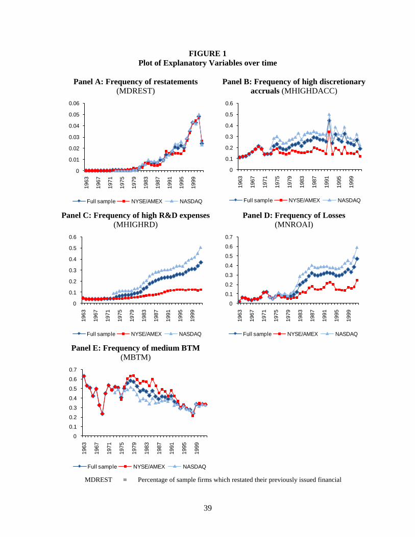
Figure 1 presents plots of the explanatory variables over time. Panel A shows the

frequency of restatements from 1962 to 2002 and shows a striking increase through the

1990’s and early 2000’s. Panel B shows the frequency of high discretionary accruals

over time, and exhibits an increasing pattern, particularly for NASDAQ firms and the

sample as a whole, over time. Panel C shows the frequency of firm-years with high R&D

expenses relative to sales, and shows a significant increase over time, and especially so

for the NASDAQ sample. Panel D shows the frequency of losses and shows an

increasing trend over time for both exchanges and the sample overall. NASDAQ firms

exhibit a significantly higher frequency of losses, beginning in the early 1980’s, climbing

to over 50% of firm-years by 2002. Panel E shows the frequency of firm-years with

book-to-market ratios in deciles 5-8, corresponding to ratios closer to 1. As panel E

shows, there is a generally declining tendency for firms to have book-to-market ratios

close to one, with firms from both exchanges exhibiting a general decline, and with

NASDAQ firms showing a lower frequency of book-to-market ratios close to one.

5. Discussion of Results

5.1 Bankruptcy Prediction Models

Panel A of Table 3 reports the estimation of the basic model developed by BMR.

The results are similar to those originally reported even though the sample has been

expanded considerably. The major findings remain the same. Consistent with prior

results, all three accounting ratios are significant and have the predicted sign.

As in the prior paper, the predicted scores are ranked and divided into deciles,

based on the combined distribution of bankrupt and non-bankrupt firm years. The

percentage of firm years in these deciles is then reported separately for year prior to

21

bankruptcy, prior years for bankrupt firms and firm-years for non-bankrupt firms. Decile

0 has the highest probability of bankruptcy.

We find that 83.45 % of bankrupt firms appear in the three lowest deciles, i.e., in

the deciles with the highest estimated probability of bankruptcy, compared to an expected

30% based on the null hypothesis of no predictive power. Consistent with prior results, in

the years before bankruptcy, the percentage of firms in the first three deciles is also

higher than expected. The percentage of earlier firm-years for firms that eventually

declare bankruptcy is also asymmetrically distributed in the highest risk deciles,

indicating that these firms had a higher probability of bankruptcy in these earlier years as

well. Cumulative density functions by year before failure (Figures 1 through 4 reported

in BMR) also indicate that the higher probability of bankruptcy was evident for as much

as five years prior to bankruptcy.

With respect to the accounting models, all three accounting variables are of the

predicted sign and are significant. Probability of default is decreasing in profitability,

increasing in leverage, and decreasing in EBITDA relative to total liabilities. The

percentage of bankrupt firm-years in the three highest bankruptcy risk deciles (i.e. deciles

0 through 2) is adopted as a convenient way of comparing predictive ability across

models and samples.

As discussed earlier, we also estimate a model that includes an indicator variable,

NROAI, for lack of profitability, and with separate slope coefficients for the loss firm-

years. Panel B of Table 3 indicates the coefficient on this indicator variable is

significantly positive, which implies the probability of bankruptcy is significantly higher

for loss firms. A coefficient of 2.296 implies that the probability of bankruptcy for a firm

22

with losses is approximately 10 times as great as when net income is positive, conditional

upon the other variables in the model.

The three accounting variables in the prediction model remain significant and of

the predicted sign for profitable firms. However, the incremental coefficients for the loss

firms are of the opposite sign and are significant, implying the combined coefficients for

the loss firms are driven toward zero. The coefficient on ROA is not significantly

different from zero for loss firms. This finding is analogous to that of Collins et al.

(1999), who find in a valuation context, the slope coefficient for loss firms is essentially

zero. However, this is somewhat more surprising in the context of bankruptcy prediction.

The percentage of bankrupt firm-years in the lowest three deciles is 80.02 percent, which

is comparable to that of the more parsimonious model.

Panel C presents the estimated coefficients for the market model. Coefficients

have the predicted signs, are significant, and are consistent with those reported in BMR.

In particular, the probability of bankruptcy is increasing in volatility of residual returns,

and decreasing in size and lagged residual return. Moreover, 82.3 percent of firms are in

the bottom 3 deciles in the year of bankruptcy, which is much greater than the 30 percent

expected under the null hypothesis of no predictive ability. The predictive ability is only

slightly higher than that of the accounting model at 80.02 percent. Virtually all of the

predictive ability of market-based variables is captured by the three accounting-based

variables.

Panel D of Table 3 reports the estimation results for a combined hazard model

that includes both accounting and market-based variables, where the accounting model is

the one originally estimated in BMR. Panel E of Table 3 reports the estimation results for

23

a combined hazard model that includes both accounting and market-based variables,

where the accounting model includes NROAI, the loss indicator variable, and NROAI is

interacted with the accounting variables. The coefficient on NROAI, 4.004, is significant

and implies that the presence of a loss implies a firm is more than 50 times as likely to

declare bankruptcy. Moreover, even in the presence of the market-based variables, the

accounting-based variables remain significant for the profitable firms. This is important

because the market-based variables reflect the total mix of information of which financial

statements are only a subset, and in principle, could subsume the predictive ability of the

accounting-based variables. Similar to the results for the accounting-based model, all of

the incremental slope coefficients are of the opposite sign, therefore driving the sum of

the respective coefficients toward zero. Despite this fact, untabulated findings indicate

that all variables are significant for loss firms, with the exception of LRSIZE.

The percentage of bankrupt firm-years in the bottom three deciles is 90.09

percent, which is higher than that for either the accounting or market-based model,

consistent with both the accounting and market variables having significant explanatory

power. Similar results are obtained for the combined model without separate slopes or

indicators but with a slightly lower predictive power of 88.57 percent (Table 3, Panel D).

Because of the significance of the NROAI indicator-based coefficients and overall

predictive results in the comprehensive model, the subsequent analyses are based on the

estimation equations including these variables.

In an efficient capital market, the market-based model would be expected to

dominate the accounting model, since the total mix of information includes financial

statements as a subset. However, the results indicate that approximately the same

24

predictive power is captured by the accounting variables. Moreover, accounting variables

provide some explanatory power not provided by market variables. The latter could

reflect misspecification of the market variables rather than evidence of market

inefficiency. Conversely, the market variables capture some information not captured by

the accounting variables. This could reflect information in the total mix of information

that does not derive from financial statements, as well as possible misspecification of the

accounting variables.

5.2 Discretionary Behavior Results

5.2.1 Earnings Restatements

In order to compare the predictive power of the models for restated and non-

restated years, we rank the hazard scores for all observations within each of the two

subsamples. These hazard scores are computed based on the pooled estimation of each of

the models (the negative ROA indicator variable is included in this estimation for the

accounting and combined models).

Table 4 contains the frequency of firms in each of the first three deciles, which

correspond to the highest probability of bankruptcy. As hypothesized, the predictive

power of the accounting model is lower for the firm-years where restatement is involved,

with only 50.45 percent of bankrupt firms in the lowest three deciles for the restatement

subsample, in contrast to 82.02 percent for non-restated years. Untabulated statistical

tests indicate this difference is significant with a probability value less than .01.9 This

finding is consistent with the contention that accounting numbers that are departures from

GAAP are of lower quality for bankruptcy prediction. Note that the identity of the

9 We assess the significance of the difference using a

2 test. In all further comparisons, we refer to a

subsample as having higher or lower predictive ability if the difference is significant with less than

probability value .01.

25

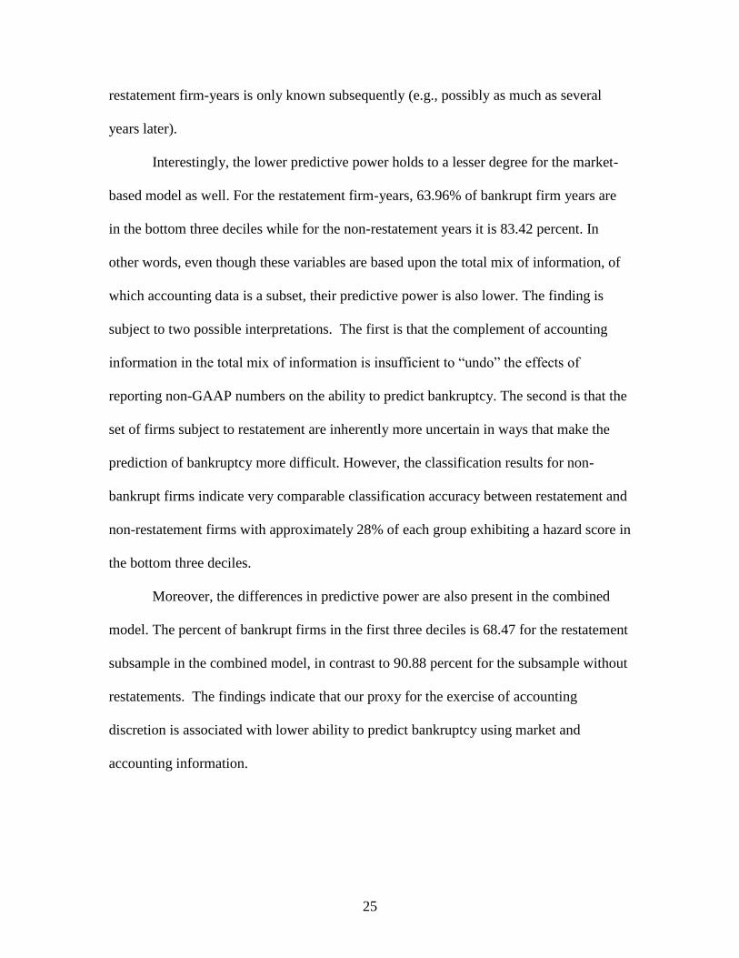
restatement firm-years is only known subsequently (e.g., possibly as much as several

years later).

Interestingly, the lower predictive power holds to a lesser degree for the market-

based model as well. For the restatement firm-years, 63.96% of bankrupt firm years are

in the bottom three deciles while for the non-restatement years it is 83.42 percent. In

other words, even though these variables are based upon the total mix of information, of

which accounting data is a subset, their predictive power is also lower. The finding is

subject to two possible interpretations. The first is that the complement of accounting

information in the total mix of information is insufficient to ―undo‖ the effects of

reporting non-GAAP numbers on the ability to predict bankruptcy. The second is that the

set of firms subject to restatement are inherently more uncertain in ways that make the

prediction of bankruptcy more difficult. However, the classification results for non-

bankrupt firms indicate very comparable classification accuracy between restatement and

non-restatement firms with approximately 28% of each group exhibiting a hazard score in

the bottom three deciles.

Moreover, the differences in predictive power are also present in the combined

model. The percent of bankrupt firms in the first three deciles is 68.47 for the restatement

subsample in the combined model, in contrast to 90.88 percent for the subsample without

restatements. The findings indicate that our proxy for the exercise of accounting

discretion is associated with lower ability to predict bankruptcy using market and

accounting information.

26

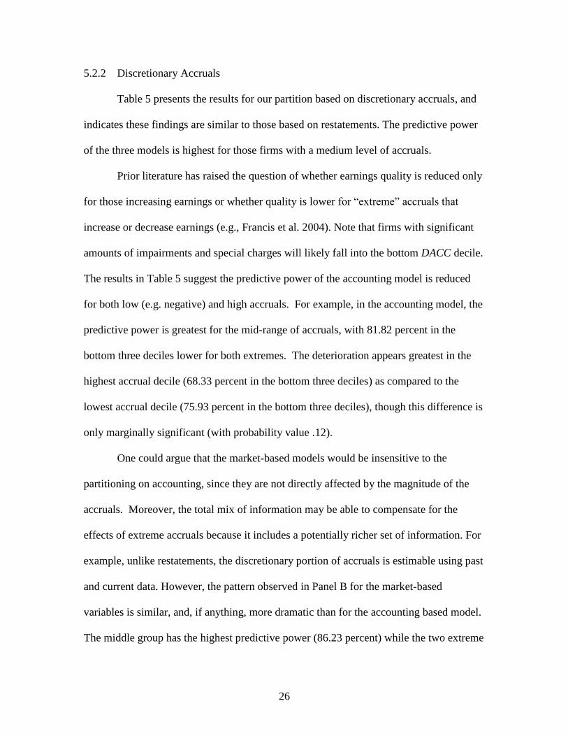
5.2.2 Discretionary Accruals

Table 5 presents the results for our partition based on discretionary accruals, and

indicates these findings are similar to those based on restatements. The predictive power

of the three models is highest for those firms with a medium level of accruals.

Prior literature has raised the question of whether earnings quality is reduced only

for those increasing earnings or whether quality is lower for ―extreme‖ accruals that

increase or decrease earnings (e.g., Francis et al. 2004). Note that firms with significant

amounts of impairments and special charges will likely fall into the bottom DACC decile.

The results in Table 5 suggest the predictive power of the accounting model is reduced

for both low (e.g. negative) and high accruals. For example, in the accounting model, the

predictive power is greatest for the mid-range of accruals, with 81.82 percent in the

bottom three deciles lower for both extremes. The deterioration appears greatest in the

highest accrual decile (68.33 percent in the bottom three deciles) as compared to the

lowest accrual decile (75.93 percent in the bottom three deciles), though this difference is

only marginally significant (with probability value .12).

One could argue that the market-based models would be insensitive to the

partitioning on accounting, since they are not directly affected by the magnitude of the

accruals. Moreover, the total mix of information may be able to compensate for the

effects of extreme accruals because it includes a potentially richer set of information. For

example, unlike restatements, the discretionary portion of accruals is estimable using past

and current data. However, the pattern observed in Panel B for the market-based

variables is similar, and, if anything, more dramatic than for the accounting based model.

The middle group has the highest predictive power (86.23 percent) while the two extreme

27

accrual deciles have the lowest (65.43 percent and 65.0 percent, respectively). Hence, the

information environment for the extreme accrual firm-years appears to be considerably

different than that of the mid-range accrual firm-years, and the differences are even more

striking for the market-based variables than for accounting-based variables. Of course, an

alternative interpretation is that extreme accruals proxy for some other underlying

economic difference, not explicitly captured by the market-based variables, that makes

bankruptcy prediction more difficult. Here, the effects for the low and high accrual

groups are symmetric.

The results in Panel C of Table 5 for the combined model show the same pattern,

less pronounced than for the market model but more pronounced than for the accounting

model, with a symmetric pattern for low and high accruals groups, as in the market

model. The most extreme positive accruals are of the lowest quality, consistent with

overstated earnings being less informative than unbiased or understated earnings.

However, consistent with ongoing research on ―earnings quality,‖ our findings indicate

extreme accruals of either sign are of lower quality with respect to bankruptcy prediction.

5.3 Unrecorded Intangible Assets

Our measure of intangible assets is based on the ratio of research and

development to sales, R&D/SALES. Firm-years are partitioned into three groups: firms

with zero R&D, firms in the top decile of R&D/SALES (High R&D), and all other firms

(Medium R&D). The basic hypothesis is that the presence of intangible assets lowers the

predictive power of the model because it represents an asset not captured by the

accounting variables. Moreover, under the total mix of information, there may be no

28

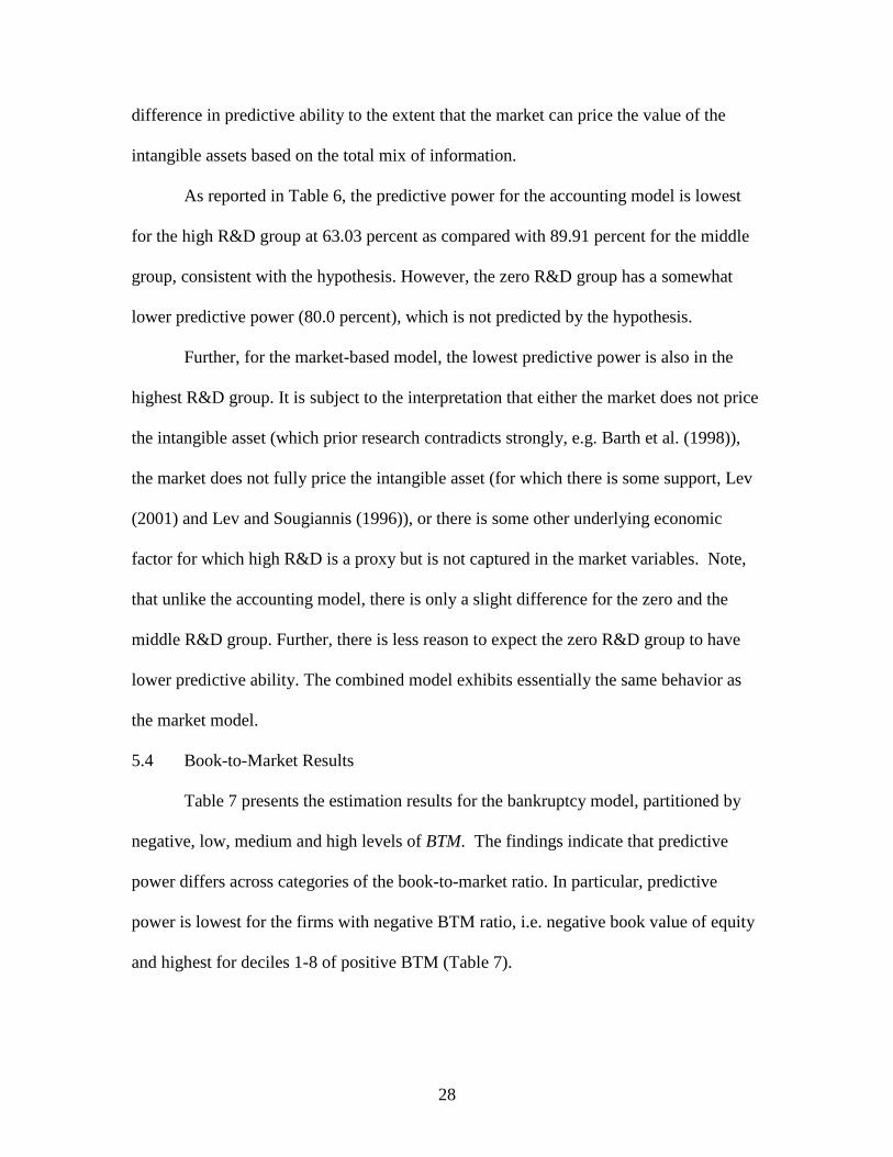
difference in predictive ability to the extent that the market can price the value of the

intangible assets based on the total mix of information.

As reported in Table 6, the predictive power for the accounting model is lowest

for the high R&D group at 63.03 percent as compared with 89.91 percent for the middle

group, consistent with the hypothesis. However, the zero R&D group has a somewhat

lower predictive power (80.0 percent), which is not predicted by the hypothesis.

Further, for the market-based model, the lowest predictive power is also in the

highest R&D group. It is subject to the interpretation that either the market does not price

the intangible asset (which prior research contradicts strongly, e.g. Barth et al. (1998)),

the market does not fully price the intangible asset (for which there is some support, Lev

(2001) and Lev and Sougiannis (1996)), or there is some other underlying economic

factor for which high R&D is a proxy but is not captured in the market variables. Note,

that unlike the accounting model, there is only a slight difference for the zero and the

middle R&D group. Further, there is less reason to expect the zero R&D group to have

lower predictive ability. The combined model exhibits essentially the same behavior as

the market model.

5.4 Book-to-Market Results

Table 7 presents the estimation results for the bankruptcy model, partitioned by

negative, low, medium and high levels of BTM. The findings indicate that predictive

power differs across categories of the book-to-market ratio. In particular, predictive

power is lowest for the firms with negative BTM ratio, i.e. negative book value of equity

and highest for deciles 1-8 of positive BTM (Table 7).

29

The behavior of the BTM ratio is complex. As the probability of bankruptcy

increases, both the book value of equity and the market value of common equity decline.

It is difficult to predict how the ratio of the two behaves in part because it is difficult to

predict which component will decline at a more rapid rate. Moreover, book value can be

negative and approaching zero, while market value cannot. In particular, the option value

of common equity can remain even as the probability of bankruptcy rises. As a result, as

losses cumulate and as book value heads towards zero, the book-to-market ratio can

approach zero (the market-to-book ratio approaches infinity).

To partially address these concerns, we partition the book-to-market ratios into

four groups: negative, low positive, medium positive, and high positive book-to-market

ratios. Table 7 shows that the same pattern of predictive power is exhibited by all three

models. The subsamples with lowest predictive power to highest are the negative BTM,

high positive BTM, low positive BTM, and medium positive BTM. The negative group

includes firm-years with negative book value and for whom the probability of bankruptcy

would be expected to be high. These are firms with negative book value but positive

market value, in part due to the option-like properties of common stock for limited

liability corporations as well as possible unrecognized intangible assets. The high

positive group includes firms for whom the market is recognizing asset impairments but

the accounting is not, or at least not to the same extent. The low positive group is a

diverse group of firm-years where either the option value of market price is causing the

market-to-book ratio to approach infinity for a low book value firm or the firms have

substantial unrecognized intangible assets. All three groups would be expected (and in

fact do) have higher than average probability of bankruptcy.

30

Overall, the results indicate that when book-to-market ratios have the greatest

departure from one, the predictive power of the bankruptcy models is weakest.

Alternatively stated, the predictive power is greater for those firm-years in which

accounting and market-based measures of value correspond more closely. Of course,

these differences in predictive ability may also reflect underlying economic factors that

are not captured by the predictive variables. This could explain why these predictive

differences are observed in the market-based models as well.

5.5 Predictive Power of Models for Loss Firms

We established that the probability of bankruptcy conditional upon a loss is

significantly higher in section 5.1. In this section, we examine whether, conditioning for

the presence of the loss, the predictive power of the models are the same for loss versus

non-loss firms. Table 8 reports the percentage of bankrupt firm-years in the bottom three

deciles for loss versus non-loss firm-years. The predictive power of the accounting

model for the loss firm years is substantially lower (70.75 percent) than for the non-loss

firm-years (77.62 percent).

This finding is consistent with the results discussed earlier which showed that,

conditional upon the presence or absence of a loss, the incremental explanatory power of

the remaining accounting and market variables is substantially lower for loss firms.

Hence, for these firms, additional variables do not provide much information for

distinguishing between the probability of failure among the set of loss firms. For non-loss

firm-years, while their conditional probability of bankruptcy is lower, the incremental

explanatory power of the additional variables is much greater in distinguishing

differences in the probability of bankruptcy.

31

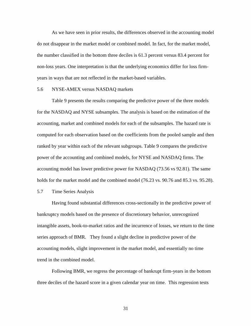
As we have seen in prior results, the differences observed in the accounting model

do not disappear in the market model or combined model. In fact, for the market model,

the number classified in the bottom three deciles is 61.3 percent versus 83.4 percent for

non-loss years. One interpretation is that the underlying economics differ for loss firm-

years in ways that are not reflected in the market-based variables.

5.6 NYSE-AMEX versus NASDAQ markets

Table 9 presents the results comparing the predictive power of the three models

for the NASDAQ and NYSE subsamples. The analysis is based on the estimation of the

accounting, market and combined models for each of the subsamples. The hazard rate is

computed for each observation based on the coefficients from the pooled sample and then

ranked by year within each of the relevant subgroups. Table 9 compares the predictive

power of the accounting and combined models, for NYSE and NASDAQ firms. The

accounting model has lower predictive power for NASDAQ (73.56 vs 92.81). The same

holds for the market model and the combined model (76.23 vs. 90.76 and 85.3 vs. 95.28).

5.7 Time Series Analysis

Having found substantial differences cross-sectionally in the predictive power of

bankruptcy models based on the presence of discretionary behavior, unrecognized

intangible assets, book-to-market ratios and the incurrence of losses, we return to the time

series approach of BMR. They found a slight decline in predictive power of the

accounting models, slight improvement in the market model, and essentially no time

trend in the combined model.

Following BMR, we regress the percentage of bankrupt firm-years in the bottom

three deciles of the hazard score in a given calendar year on time. This regression tests

32

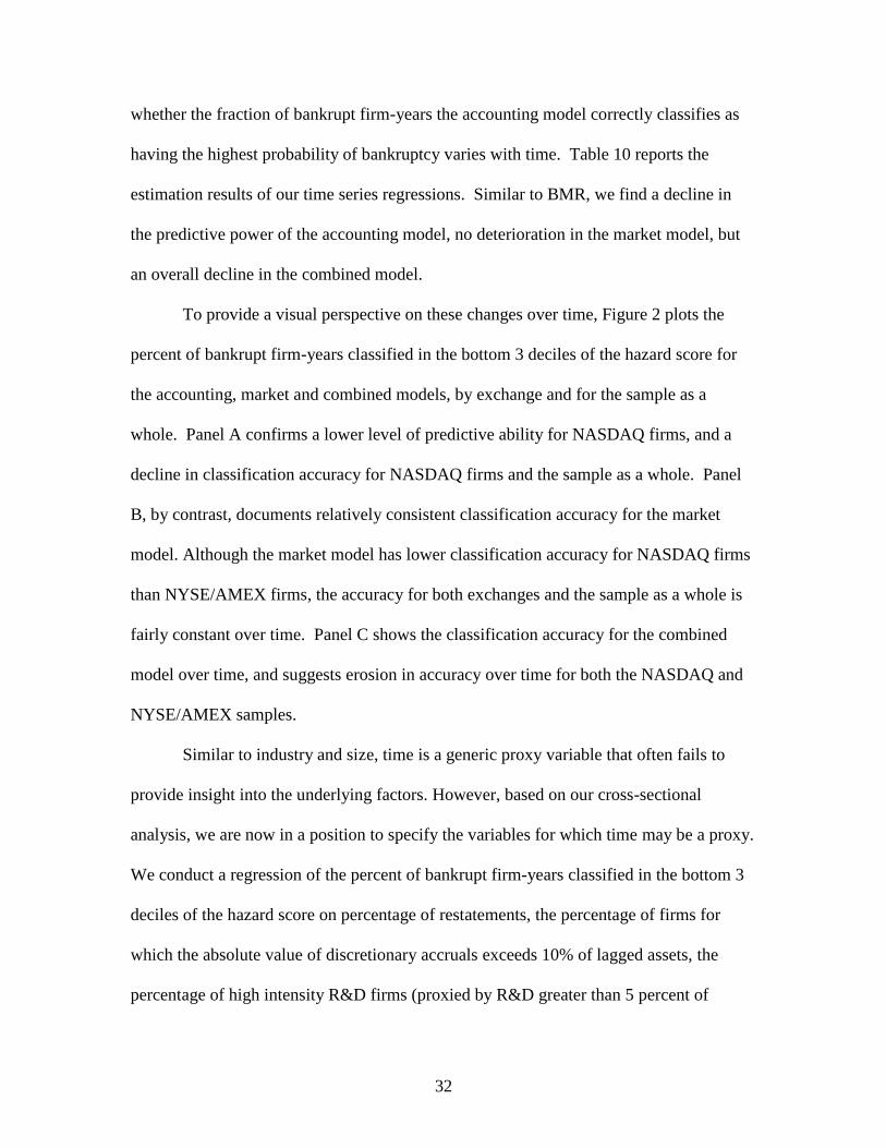
whether the fraction of bankrupt firm-years the accounting model correctly classifies as

having the highest probability of bankruptcy varies with time. Table 10 reports the

estimation results of our time series regressions. Similar to BMR, we find a decline in

the predictive power of the accounting model, no deterioration in the market model, but

an overall decline in the combined model.

To provide a visual perspective on these changes over time, Figure 2 plots the

percent of bankrupt firm-years classified in the bottom 3 deciles of the hazard score for

the accounting, market and combined models, by exchange and for the sample as a

whole. Panel A confirms a lower level of predictive ability for NASDAQ firms, and a

decline in classification accuracy for NASDAQ firms and the sample as a whole. Panel

B, by contrast, documents relatively consistent classification accuracy for the market

model. Although the market model has lower classification accuracy for NASDAQ firms

than NYSE/AMEX firms, the accuracy for both exchanges and the sample as a whole is

fairly constant over time. Panel C shows the classification accuracy for the combined

model over time, and suggests erosion in accuracy over time for both the NASDAQ and

NYSE/AMEX samples.

Similar to industry and size, time is a generic proxy variable that often fails to

provide insight into the underlying factors. However, based on our cross-sectional

analysis, we are now in a position to specify the variables for which time may be a proxy.

We conduct a regression of the percent of bankrupt firm-years classified in the bottom 3

deciles of the hazard score on percentage of restatements, the percentage of firms for

which the absolute value of discretionary accruals exceeds 10% of lagged assets, the

percentage of high intensity R&D firms (proxied by R&D greater than 5 percent of

33

sales), the frequency of book-to-market values close to 1, and the percentage of loss firms

in a given calendar year. As reported in Panel A of Table 10, all of the explanatory

variables are highly correlated making individual contributions difficult to assess.

However, Panel B shows the accounting model’s lower predictive power occurs in years

when there is a larger frequency of restatements, a relatively large amount of

discretionary accruals, relatively high research and development intensity, a higher

frequency of firms with book-to-market ratios further from one, and a higher frequency

of losses. This evidence is consistent with the cross-sectional analysis and helps to

identify at least some of the factors associated with the observed decline over time in

predictive power. Interestingly, as Panel C shows, the market model exhibits no such

decline over time. However, as Panel D shows, the differential predictive ability of the

combined model declines significantly over time. This finding suggests that the erosion

in predictive ability of financial ratios was not offset by information reflected in the

market-related variables.

5.8 Sensitivity analysis

In the above specifications, the baseline hazard is assumed to be constant across

time. Bankruptcy rates are likely correlated, however, with fluctuations in economic

activity. As a result, cross-sectional correlation of errors may be a concern in the above

regressions, resulting in upward biased standard errors. In order to circumvent this

problem, and following Hillegeist et al. (2004), we use the overall frequency of

bankruptcy in a given year to proxy for the baseline hazard (this rate is calculated as the

ratio between the number of bankruptcies and the total number of firms in the sample

over the previous 12 months and is expressed as a percentage). In unreported results, the

34

annual bankruptcy rate is significant in all specifications, suggesting that the baseline

hazard rate provides information that is incremental to the accounting and market

variables.

In addition, we combine the market-based models into a Black-Scholes-Merton

model of bankruptcy. We use the SAS code provided in the appendix of Hillegeist et al.

(2004) to estimate the BSM probability of bankruptcy, defined as the probability that the

market value of assets is less than the face value of liabilities. Also following this study,

the BSM probability of bankruptcy is then transformed into a score using the inverse

logistic function. In unreported results, this variable is significant in all specifications.10

In the basic specification, that merely includes the BSM score and the annual bankruptcy

rate, the BSM score has a coefficient close to that reported in Table 5 of Hillegeist et al.

(2004). The BSM model performs about as well as the market-based models. The

accounting variables are still significant when the market variables are replaced by the

BSM score, suggesting that the accounting information has incremental explanatory

power with respect to this variable.

In summary, neither alternative specification alters our basic conclusions

regarding discretionary accruals, restatements, research and development intensity, book-

to-market and losses.

6. Concluding Remarks

The goal of this paper is to explore the effect of cross-sectional and time-series

differences in discretion, unrecognized intangible assets, book-to market ratios, and

10

In the basic specification that merely includes the BSM score and the annual bankruptcy rate, both

variables have magnitudes that are comparable to Hillegeist, Keating, Cram and Lundstedt (2004). In

particular, the coefficient on the BSM score is 0.31 (vs. 0.27) and on the annual rate 0.43 (vs. 0.54)

35

incidence of losses on the predictive ability of financial ratios for bankruptcy. We find

that all of our proxies for the exercise of discretion in financial reporting are associated

with a significant deterioration in the predictive power of the accounting-based model.

In addition, the presence of discretion impairs the predictive ability of not only the

accounting-based model but also the market-based and combined model. In other words,

the total mix of information reflected in market-based variables, of which accounting data

are a subset, does not offset or compensate for the effects of discretion.

We also find that the presence of intangible assets, as measured by research and

development intensity, has a systematic effect on predictive ability. In particular, the

predictive power of the accounting-based model is lower for firms with a high degree of

research and development intensity.

We also examine the predictive power of the bankruptcy models across various

categories of the book-to market ratio. Predictive power varies across book-to-market

classes but not in a monotonic fashion. Firm-years with low to medium positive book-to-

market ratios are most informative, consistent with more informative financial statements

results when the book value of equity is closer to the market value of equity. Firm-years

with high book-to-market ratios are next most informative, while the financial statements

of firms with negative ratios of book-to-market are least informative. The findings are

consistent with the contention that when financial statements fail to recognize changes in

asset values, either in the form of intangible assets or abandonment options, the

predictive ability of financial ratios is impaired. These finding have potential implications

for the use of the book-to-market ratios in other contexts as well.

36

We find that the incidence of a loss significantly increases the conditional

probability of bankruptcy. However, we also find that the predictive power of the

bankruptcy model for loss firm-years tends to be lower than for non-loss firm-years

because of a deterioration in the incremental explanatory power of the remaining

variables.

Finally, we return to the time series analysis to attempt to improve our

understanding for the decline in the predictive power of the accounting model over time.

We find that there is a significant time trend in the frequency of restatements, of larger

magnitudes of discretionary accruals, of greater R&D intensity, of book-to-market ratios

that are further from one, and of losses. These variables are individually significant in

explaining differences in predictive ability over time. However, because of high

correlation with each other, it is difficult to isolate individual, incremental effects.

In the cross-sectional context, in most cases the market model also exhibited

lower predictive power for the same categories of firm-years as the accounting model.

However, unlike the accounting model, the market model exhibits no declining time trend

and differences in predictive power over time are uncorrelated with our partitioning

variables. These findings suggest that the changes in financial reporting attributes we

document contribute to less informative financial ratios, as assessed by bankruptcy

prediction. Furthermore, the findings that the combined model exhibits a declining time

trend in predictive power and that this is associated with our partitioning variables

indicate that the market variables included in our market and combined models did not

compensate for the loss of information over time.

37

References

Barth, M., M. Clement, G. Foster, and R. Kasznik 1998. Brand values and capital market

valuation. Review of Accounting Studies 3: 41-68.

Basu, S. 1997. The conservatism principle and the asymmetric timeliness of earnings.

Journal of Accounting and Economics 24 (1): 3-37.

Beaver, W. H. and E. Engel. 1996. Discretionary behavior with respect to allowances for

loan losses and the behavior of security prices. Journal of Accounting and Economics

(22): 177-206.

Beaver, W. H., 2002. Perspectives on recent capital market research. The Accounting

Review 77 (2): 453-474.

Beaver, W.H., M. McNichols, and J. Rhie. 2005. Have financial statements become less

informative? Evidence from the ability of financial ratios to predict bankruptcy. Review

of Accounting Studies 10 (1): 93-122.

Bonner, S., Z. Palmrose, and S. Young. 1998. Fraud type and auditor Litigation: An

analysis of SEC accounting and auditing enforcement releases. The Accounting Review

73 (4): 503-552.

Bradshaw, M., and R. Sloan. 2002. GAAP versus the street: An empirical assessment of

two alternative definitions of earnings. Journal of Accounting Research 40 (1): 41-66.

Chava, S., and R. Jarrow. 2004. Bankruptcy prediction with industry effects. Review of

Finance 8 (4): 537-569.

Collins, D., M. Pincus, and H. Xie. 1999. Equity valuation and negative earnings: The

role of book value of equity. The Accounting Review 74 (1): 29-61.

Dechow, P., R. Sloan, and A. Sweeney. 1995. Detecting earnings management. The

Accounting Review 70 (2): 193-225.

Dechow, P., and C. Schrand. 2004. Earnings Quality. CFA Digest 34 (4): 82-85.

Financial Accounting Standards Board (FASB). 2001. Accounting for the Impairment or

Disposal of Long-Lived Assets. FASB Statement No. 144. Stamford, Conn.: FASB.

Francis, J., R. LaFond, P. Olsson, and K. Schipper. 2004. Cost of equity and earnings

attributes. The Accounting Review 79 (4): 967-1010.

Francis, J., R. LaFond, P. Olsson, and K. Schipper. 2005. The market pricing of accruals

quality. Journal of Accounting and Economics 39 (2): 295-327.

38

Givoly, D., and C. Hayn. 2000. The changing time-series properties of earnings, cash

flows and accruals: Has financial reporting become more conservative? Journal of

Accounting and Economics 29 (3): 287-320.

Graham, B., and D. Dodd. 1934. Security Analysis. New York, NY: McGraw Hill.

Hayn, C. 1995. The information content of losses. Journal of Accounting and Economics

20 (2): 125-153.

Hillegeist, S., E. Keating, D. Cram, and K. Lundstedt. 2004. Assessing the probability of

bankruptcy. Review of Accounting Studies 9 (1): 1573-7136.

Kasznik, R. 1999. On the association between voluntary disclosure and earnings

management. Journal of Accounting Research 37 (1): 57-81.

Lev, B., and T. Sougiannis. 1996. The capitalization, amortization, and value-relevance

of R&D. Journal of Accounting and Economics 21 (1): 107-138.

Lev, B., and P. Zarowin. 1999. The boundaries of financial reporting and how to extend

them. Journal of Accounting Research 37 (2): 353–386.

Lev, B. 2001. Intangibles: Management, Measurement, and Reporting. Washington,

D.C.: Brookings Institution Press.

McNichols, M. 2000. Research design issues in earnings management studies. Journal of

Accounting and Public Policy 19: 313-345.

Wahlen, J. 1994. The nature of information in commercial bank loan loss disclosures.

The Accounting Review 69 (3): 455-478.

Watts, R., and J. Zimmerman. 1990. Positive accounting theory: A ten year perspective.

The Accounting Review 65 (1): 131–156.

39

FIGURE 1

Plot of Explanatory Variables over time

Panel A: Frequency of restatements (MDREST)

Panel B: Frequency of high discretionary

accruals (MHIGHDACC)

0

0.01

0.02

0.03

0.04

0.05

0.06

1963

1967

1971

1975

1979

1983

1987

1991

1995

1999

Full sample NYSE/AMEX NASDAQ

0

0.1

0.2

0.3

0.4

0.5

0.6

1963

1967

1971

1975

1979

1983

1987

1991

1995

1999

Full sample NYSE/AMEX NASDAQ

Panel C: Frequency of high R&D expenses

(MHIGHRD) Panel D: Frequency of Losses

(MNROAI)

0

0.1

0.2

0.3

0.4

0.5

0.6

1963

1967

1971

1975

1979

1983

1987

1991

1995

1999

Full sample NYSE/AMEX NASDAQ

0

0.1

0.2

0.3

0.4

0.5

0.6

0.71963

1967

1971

1975

1979

1983

1987

1991

1995

1999

Full sample NYSE/AMEX NASDAQ

Panel E: Frequency of medium BTM

(MBTM)

0

0.1

0.2

0.3

0.4

0.5

0.6

0.7

1963

1967

1971

1975

1979

1983

1987

1991

1995

1999

Full sample NYSE/AMEX NASDAQ

MDREST = Percentage of sample firms which restated their previously issued financial

40

statements for year t;

MROAI = Percentage of loss firms in year t;

MHIGHDACC = Percentage of firms in year t whose discretionary accruals represent more than 10%

of lagged assets;

MHIGHRD = Percentage of firms in year t whose R&D expenses represent more than 5% of sales;

MBTM = Percentage of firms with BTM ratio in deciles 5-8 of positive BTM.

41

FIGURE 2

Percentage of bankrupt firms in the top 3 deciles of predicted hazard rate over timea

Panel A: Accounting Model

0.5

0.55

0.6

0.65

0.7

0.75

0.8

0.85

0.9

0.95

1

1964

1970

1972

1974

1976

1978

1980

1982

1984

1986

1988

1990

1992

1994

1996

1998

2000

2002

Full sample NYSE/AMEX NASDAQ

Panel B: Market Model

0

0.2

0.4

0.6

0.8

1

1964

1970

1972

1974

1976

1978

1980

1982

1984

1986

1988

1990

1992

1994

1996

1998

2000

2002

Full sample NYSE/AMEX NASDAQ

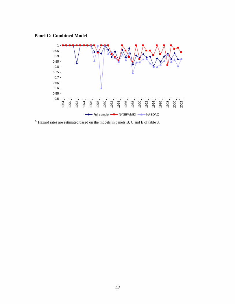
42

Panel C: Combined Model

0.5

0.55

0.6

0.65

0.7

0.75

0.8

0.85

0.9

0.95

1

1964

1970

1972

1974

1976

1978

1980

1982

1984

1986

1988

1990

1992

1994

1996

1998

2000

2002

Full sample NYSE/AMEX NASDAQ

a. Hazard rates are estimated based on the models in panels B, C and E of table 3.

43

TABLE 1

Sample Selection

Number of firms Number of firm years

bankrupt

non-

bankrupt Total bankrupt

non-

bankrupt Total

1,857

Firms not listed in NYSE, AMEX or NASDAQ (54)

1,803

Financial and utilities firms (179)

Number of firms 1,624

Firms with no asset information (12)

Firms with available asset information 1,612

Firms for which accounting model data is

unavailable (211)

1,401

Firms for which market model data is unavailable (14)

1,387

Firms for which accounting or market data is

unavailable in the bankruptcy year, but available for

at least one of the years prior to bankruptcy (136)

Pooled Sample

year of bankruptcy 1,251 1,251

earlier bankrupt years 1,387 9,989

total 1,387 12,978 14,365 11,240 124,215 135,455

Transition years 164 1,178 1,342

NYSE/AMEX

year of bankruptcy 487 487

earlier bankrupt years 560 5,775

total 560 4,297 4,857 6,262 57,927 64,189

NASDAQ

year of bankruptcy 749 749

earlier bankrupt years 972 4,065

total 972 9,706 10,678 4,814 65,110 69,924

Firm for which accounting variables are available

(after filling in)

Firms listed in NYSE, AMEX or NASDAQ with

available identifiers

Number of bankrupt firms used in the analysis

Firms with available PERMNO and GVKEY

Our final sample includes bankrupt and non-bankrupt firms listed on NYSE/AMEX or NASDAQ from

1962-2002 (the first years of the sample only include NYSE/AMEX firms, as the NASDAQ subsample

only starts in 1973). It is the result of the combination of a sample of bankrupt firms generously provided

by Chava and Jarrow and the sample of bankrupt firms in BMR. There were 2,014 observations referring to

1967 firms in the Chava Jarrow Sample. We were able to match 1,780 of these firms to Compustat and

CRSP. 504 of these matched firms were also included in the BMR sample (cf. BMR, table 1), while 1,276

firms were not. Also 77 firms in the BMR sample were not in the Chava Jarrow sample. As a result, we

obtained a sample of 1,857 firms with available PERMNO and GVKEY identifiers. This table describes the

process by which we built the final sample used in the regression analysis, departing from these 1,857

bankrupt firms. Firm year observations are split between the NYSE/AMEX and NASDAQ subsamples,

with transition years being left out of both samples. Note that the sum of the number of firms in the two

subsamples (presented in the first three columns) is higher than the number of firms in the pooled sample.

This occurs because firms which have transitioned from one stock exchange to the other will show up in

both subsamples.

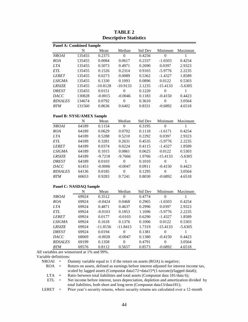
44

TABLE 2

Descriptive Statistics

Panel A: Combined Sample

N Mean Median Std Dev Minimum Maximum

NROAI 135455 0.2375 0 0.4256 0 1

ROA 135455 0.0084 0.0617 0.2337 -1.6503 0.4254

LTA 135455 0.5073 0.4971 0.2690 0.0397 2.9323

ETL 135455 0.1526 0.2314 0.9165 -5.9776 2.2235

LERET 135455 0.0273 0.0089 0.5362 -1.4327 1.8589

LSIGMA 135455 0.1330 0.1093 0.0896 0.0122 0.5303

LRSIZE 135455 -10.8128 -10.9133 2.1235 -15.4133 -5.6305

DREST 135455 0.0151 0 0.1220 0 1

DACC 130828 -0.0015 -0.0046 0.1183 -0.4150 0.4423

RDSALES 134674 0.0792 0 0.3610 0 3.0564

BTM 131560 0.8636 0.6402 0.8331 -0.6892 4.6518

Panel B: NYSE/AMEX Sample

N Mean Median Std Dev Minimum Maximum

NROAI 64189 0.1154 0 0.3195 0 1

ROA 64189 0.0629 0.0702 0.1118 -1.6171 0.4254

LTA 64189 0.5288 0.5210 0.2292 0.0397 2.9323

ETL 64189 0.3281 0.2631 0.4535 -5.9776 2.2235

LERET 64189 0.0374 0.0224 0.4115 -1.4327 1.8589

LSIGMA 64189 0.1015 0.0861 0.0625 0.0122 0.5303

LRSIZE 64189 -9.7218 -9.7666 1.9766 -15.4133 -5.6305

DREST 64189 0.0103 0 0.1010 0 1

DACC 61453 -0.0006 -0.0047 0.0911 -0.4150 0.4423

RDSALES 64136 0.0185 0 0.1295 0 3.0564

BTM 60653 0.9283 0.7241 0.8030 -0.6892 4.6518

Panel C: NASDAQ Sample

N Mean Median Std Dev Minimum Maximum

NROAI 69924 0.3512 0 0.4774 0 1

ROA 69924 -0.0424 0.0468 0.2965 -1.6503 0.4254

LTA 69924 0.4871 0.4637 0.2996 0.0397 2.9323

ETL 69924 -0.0103 0.1853 1.1696 -5.9776 2.2235

LERET 69924 0.0177 -0.0103 0.6290 -1.4327 1.8589

LSIGMA 69924 0.1618 0.1376 0.1006 0.0122 0.5303

LRSIZE 69924 -11.8156 -11.8415 1.7319 -15.4133 -5.6305

DREST 69924 0.0194 0 0.1381 0 1

DACC 68069 -0.0028 -0.0047 0.1380 -0.4150 0.4423

RDSALES 69199 0.1358 0 0.4791 0 3.0564

BTM 69576 0.8112 0.5657 0.8573 -0.6892 4.6518 All variables are winsorized at 1% and 99%.

Variable definitions:

NROAI = Dummy variable equal to 1 if the return on assets (ROA) is negative;

ROA = Return on assets, defined as earnings before interest adjusted for interest income tax,

scaled by lagged assets (Compustat data172+data15*(1-taxrate))/lagged data6);

LTA = Ratio between total liabilities and total assets (Compustat data 181/data 6);

ETL = Net income before interest, taxes depreciation, depletion and amortization divided by

total liabilities, both short and long term (Compustat data13/data181);

LERET = Prior year’s security returns, where security returns are calculated over a 12-month

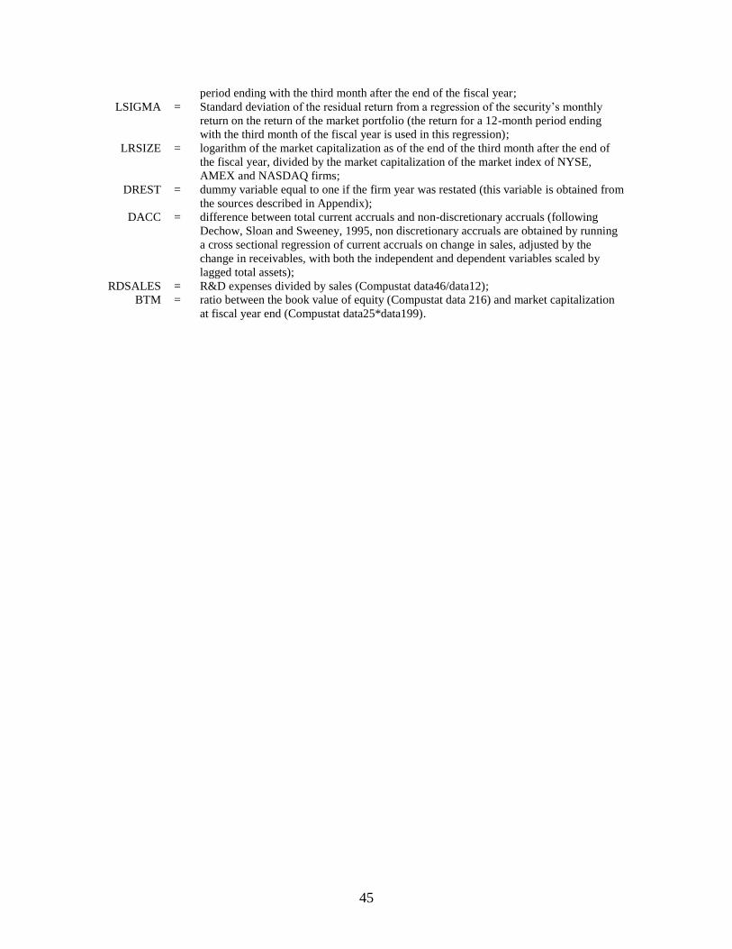
45

period ending with the third month after the end of the fiscal year;

LSIGMA = Standard deviation of the residual return from a regression of the security’s monthly

return on the return of the market portfolio (the return for a 12-month period ending

with the third month of the fiscal year is used in this regression);

LRSIZE = logarithm of the market capitalization as of the end of the third month after the end of

the fiscal year, divided by the market capitalization of the market index of NYSE,

AMEX and NASDAQ firms;

DREST = dummy variable equal to one if the firm year was restated (this variable is obtained from

the sources described in Appendix);

DACC = difference between total current accruals and non-discretionary accruals (following

Dechow, Sloan and Sweeney, 1995, non discretionary accruals are obtained by running

a cross sectional regression of current accruals on change in sales, adjusted by the

change in receivables, with both the independent and dependent variables scaled by

lagged total assets);

RDSALES = R&D expenses divided by sales (Compustat data46/data12);

BTM = ratio between the book value of equity (Compustat data 216) and market capitalization

at fiscal year end (Compustat data25*data199).

46

TABLE 3

Hazard Model Estimationa

Panel A: Original Accounting Model

Coefficients Chi-Square p value

Intercept -5.7282 14269.19 <.0001

ROA -0.6722 41.42 <.0001

LTA 1.6444 871.37 <.0001

ETL -0.1374 14.83 0.0001

year of bankruptcy Earlier bankrupt years Non bankrupt firms

N Cumulative (%) N Cumulative (%) N Cumulative (%)

0 641 51.24 1721 17.23 11164 8.99

1 263 72.26 1666 33.91 11618 18.34

2 140 83.45 1297 46.89 12113 28.09

3 58 88.09 1040 57.3 12450 38.12

4 55 92.49 941 66.72 12552 48.22

5 42 95.84 808 74.81 12700 58.44

6 22 97.6 779 82.61 12753 68.71

7 16 98.88 671 89.33 12857 79.06

8 7 99.44 606 95.39 12940 89.48

9 7 100 460 100 13068 100

Total 1251 9989 124215

Panel B:Accounting Loss Model

Coefficients Chi-Square p-value

Intercept -6.6067 3220.79 <.0001

NROAI 2.296 310.02 <.0001

ROA -5.747 30.52 <.0001

LTA 2.7824 426.98 <.0001

ETL -0.8941 102.43 <.0001

NROAI*ROA 5.9017 31.66 <.0001

NROAI*LTA -1.497 101.06 <.0001

NROAI*ETL 1.134 121.05 <.0001

Year of bankruptcy Earlier bankrupt years Non bankrupt firms

N Cumulative (%) N Cumulative (%) N Cumulative (%)

0 708 56.59 1766 17.68 11052 8.9

1 195 72.18 1355 31.24 11997 18.56

2 98 80.02 1145 42.71 12307 28.46

3 112 88.97 1283 55.55 12153 38.25

4 51 93.05 972 65.28 12525 48.33

5 29 95.36 924 74.53 12597 58.47

6 26 97.44 763 82.17 12765 68.75

7 13 98.48 692 89.1 12839 79.08

8 10 99.28 621 95.31 12922 89.49

9 9 100 468 100 13058 100

Total 1251 9989 124215

47

TABLE 3- continued

Panel C: Market Model

Coefficients Chi-Square p value

Intercept -8.0171 1462.91 <.0001

LERET -1.506 827.71 <.0001

LSIGMA 5.9363 445.44 <.0001

LRSIZE -0.1728 83.10 <.0001

year of bankruptcy Earlier bankrupt years Non bankrupt firms

N Cumulative (%) N Cumulative (%) N Cumulative (%)

0 628 50.2 1372 13.74 11526 9.28

1 242 69.54 1353 27.28 11952 18.9

2 160 82.33 1210 39.39 12180 28.71

3 92 89.69 1137 50.78 12319 38.62

4 50 93.69 995 60.74 12503 48.69

5 26 95.76 933 70.08 12591 58.83

6 24 97.68 845 78.54 12685 69.04

7 7 98.24 758 86.12 12779 79.33

8 12 99.2 703 93.16 12838 89.66

9 10 100 683 100 12842 100

Total 1251 9989 124215

Panel D: Original Combined Model

Coefficients Chi-Square p value

Intercept -8.5275 1598.14 <.0001

ROA 0.5354 18.83 <.0001

LTA 1.4483 560.46 <.0001

ETL 0.0625 2.14 0.1433

LERET -1.5057 741.90 <.0001

LSIGMA 5.9298 381.34 <.0001

LRSIZE -0.1431 55.47 <.0001

year of bankruptcy Earlier bankrupt years Non bankrupt firms

N Cumulative (%) N Cumulative (%) N Cumulative (%)

0 757 60.51 1661 16.63 11108 8.94

1 232 79.06 1410 30.74 11905 18.53

2 119 88.57 1292 43.68 12139 28.3

3 50 92.57 1146 55.15 12352 38.24

4 38 95.6 969 64.85 12541 48.34

5 15 96.8 850 73.36 12685 58.55

6 19 98.32 754 80.91 12781 68.84

7 4 98.64 685 87.77 12855 79.19

8 9 99.36 564 93.41 12980 89.64

9 8 100 658 100 12869 100

Total 1251 9989 124215

48

TABLE 3- continued

Panel E:Combined Loss Model

Coefficients Chi-Square p-value

Intercept -9.43 629.90 <.0001

NROAI 4.004 73.17 <.0001

ROA -2.6072 8.88 0.0029

LTA 2.3559 280.81 <.0001

ETL -0.5587 26.29 <.0001

LERET -1.8672 304.49 <.0001

LSIGMA 7.7992 153.98 <.0001

LRSIZE -0.1289 14.48 0.0001

NROAI*ROA 3.2388 13.33 0.0003

NROAI*LTA -1.1697 56.00 <.0001

NROAI*ETL 0.867 49.40 <.0001

NROAI*LERET 0.6829 30.49 <.0001

NROAI*LSIGMA -3.586 25.01 <.0001

NROAI*LRSIZE 0.1271 9.40 0.0022

Year of bankruptcy Earlier bankrupt years Non bankrupt firms

N Cumulative (%) N Cumulative (%) N Cumulative (%)

0 798 63.79 1740 17.42 10988 8.85

1 216 81.06 1469 32.13 11862 18.4

2 113 90.09 1232 44.46 12205 28.22

3 51 94.16 1139 55.86 12358 38.17

4 29 96.48 1038 66.25 12481 48.22

5 19 98 894 75.2 12637 58.39

6 7 98.56 731 82.52 12816 68.71

7 9 99.28 650 89.03 12885 79.08

8 4 99.6 601 95.04 12948 89.51

9 5 100 495 100 13035 100

Total 1251 9989 124215 a N=135,455.

This table presents the estimation results for different hazard models for the full sample of bankrupt and

non-bankrupt firm years and the distribution of firms across deciles of the predicted probability of

bankruptcy, ranked from the highest probability (decile 0) to lowest probability (decile 9). Panel A presents

this analysis for the original accounting-based hazard model in BMR. Panel B modifies this model to

include a dummy variable for negative ROA (NROAI) and its interactions with the remaining accounting

variables. Panels C and D contain the analysis for the market-based hazard model and the combined model

originally included in BMR. Panel E modifies the combined model to include NROAI and respective

interactions.

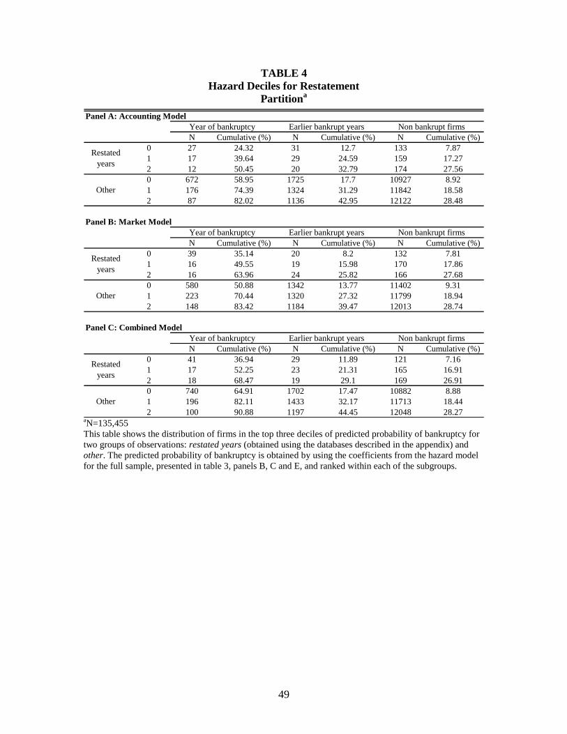
49

TABLE 4

Hazard Deciles for Restatement

Partitiona

Panel A: Accounting Model

Year of bankruptcy Earlier bankrupt years Non bankrupt firms

N Cumulative (%) N Cumulative (%) N Cumulative (%)

0 27 24.32 31 12.7 133 7.87

1 17 39.64 29 24.59 159 17.27

2 12 50.45 20 32.79 174 27.56

0 672 58.95 1725 17.7 10927 8.92

1 176 74.39 1324 31.29 11842 18.58

2 87 82.02 1136 42.95 12122 28.48

Panel B: Market Model

Year of bankruptcy Earlier bankrupt years Non bankrupt firms

N Cumulative (%) N Cumulative (%) N Cumulative (%)

0 39 35.14 20 8.2 132 7.81

1 16 49.55 19 15.98 170 17.86

2 16 63.96 24 25.82 166 27.68

0 580 50.88 1342 13.77 11402 9.31

1 223 70.44 1320 27.32 11799 18.94

2 148 83.42 1184 39.47 12013 28.74

Panel C: Combined Model

Year of bankruptcy Earlier bankrupt years Non bankrupt firms

N Cumulative (%) N Cumulative (%) N Cumulative (%)

0 41 36.94 29 11.89 121 7.16

1 17 52.25 23 21.31 165 16.91

2 18 68.47 19 29.1 169 26.91

0 740 64.91 1702 17.47 10882 8.88

1 196 82.11 1433 32.17 11713 18.44

2 100 90.88 1197 44.45 12048 28.27

Restated

years

Other

Restated

years

Other

Restated

years

Other

aN=135,455

This table shows the distribution of firms in the top three deciles of predicted probability of bankruptcy for

two groups of observations: restated years (obtained using the databases described in the appendix) and

other. The predicted probability of bankruptcy is obtained by using the coefficients from the hazard model

for the full sample, presented in table 3, panels B, C and E, and ranked within each of the subgroups.

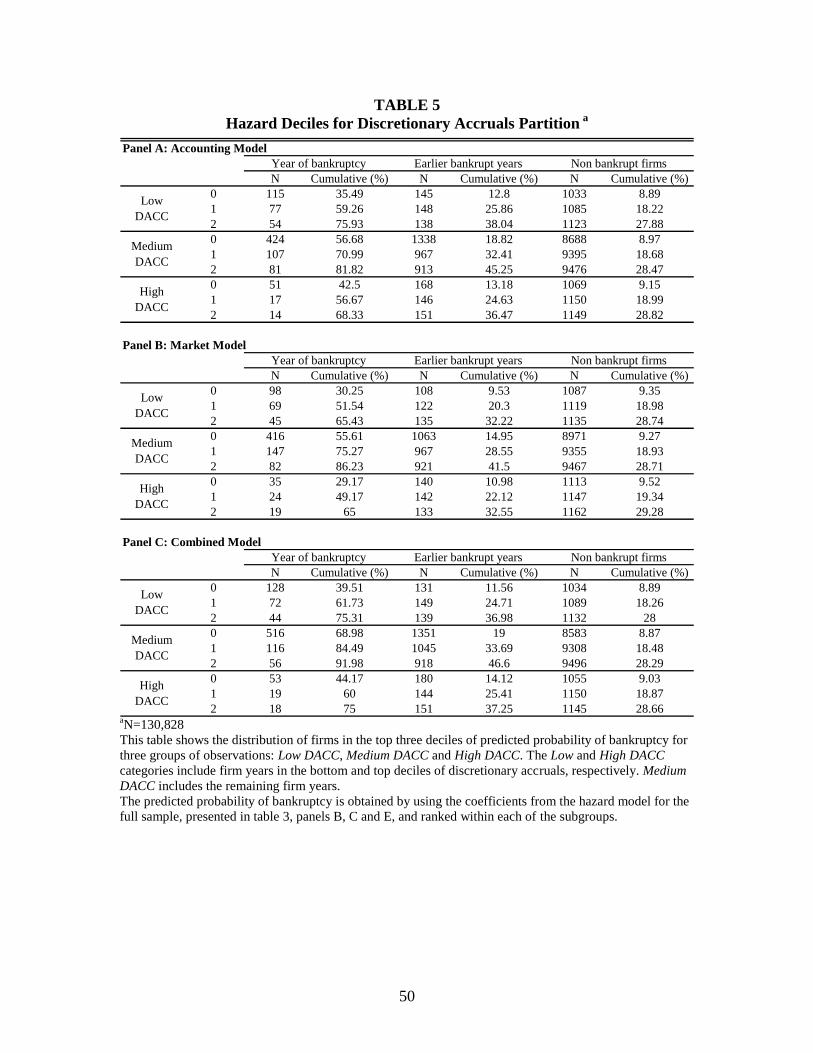
50

TABLE 5

Hazard Deciles for Discretionary Accruals Partition a

Panel A: Accounting Model

Year of bankruptcy Earlier bankrupt years Non bankrupt firms

N Cumulative (%) N Cumulative (%) N Cumulative (%)

0 115 35.49 145 12.8 1033 8.89

1 77 59.26 148 25.86 1085 18.22

2 54 75.93 138 38.04 1123 27.88

0 424 56.68 1338 18.82 8688 8.97

1 107 70.99 967 32.41 9395 18.68

2 81 81.82 913 45.25 9476 28.47

0 51 42.5 168 13.18 1069 9.15

1 17 56.67 146 24.63 1150 18.99

2 14 68.33 151 36.47 1149 28.82

Panel B: Market Model

Year of bankruptcy Earlier bankrupt years Non bankrupt firms

N Cumulative (%) N Cumulative (%) N Cumulative (%)

0 98 30.25 108 9.53 1087 9.35

1 69 51.54 122 20.3 1119 18.98

2 45 65.43 135 32.22 1135 28.74

0 416 55.61 1063 14.95 8971 9.27

1 147 75.27 967 28.55 9355 18.93

2 82 86.23 921 41.5 9467 28.71

0 35 29.17 140 10.98 1113 9.52

1 24 49.17 142 22.12 1147 19.34

2 19 65 133 32.55 1162 29.28

Panel C: Combined Model

Year of bankruptcy Earlier bankrupt years Non bankrupt firms

N Cumulative (%) N Cumulative (%) N Cumulative (%)

0 128 39.51 131 11.56 1034 8.89

1 72 61.73 149 24.71 1089 18.26

2 44 75.31 139 36.98 1132 28

0 516 68.98 1351 19 8583 8.87

1 116 84.49 1045 33.69 9308 18.48

2 56 91.98 918 46.6 9496 28.29

0 53 44.17 180 14.12 1055 9.03

1 19 60 144 25.41 1150 18.87

2 18 75 151 37.25 1145 28.66

High

DACC

Medium

DACC

High

DACC

Low

DACC

Medium

DACC

Low

DACC

Medium

DACC

High

DACC

Low

DACC

aN=130,828

This table shows the distribution of firms in the top three deciles of predicted probability of bankruptcy for

three groups of observations: Low DACC, Medium DACC and High DACC. The Low and High DACC

categories include firm years in the bottom and top deciles of discretionary accruals, respectively. Medium

DACC includes the remaining firm years.

The predicted probability of bankruptcy is obtained by using the coefficients from the hazard model for the

full sample, presented in table 3, panels B, C and E, and ranked within each of the subgroups.

51

TABLE 6

Hazard Deciles for R&D Partitiona

Panel A: Accounting Model

Year of bankruptcy Earlier bankrupt years Non bankrupt firms

N Cumulative (%) N Cumulative (%) N Cumulative (%)

0 425 52.8 893 16.48 4545 8.64

1 140 70.19 690 29.22 5058 18.25

2 79 80 672 41.62 5139 28.02

0 200 61.73 761 18.44 5295 9.08

1 66 82.1 595 32.86 5617 18.72

2 25 89.81 563 46.5 5696 28.49

0 41 34.45 53 11.94 1244 9.61

1 18 49.58 61 25.68 1272 19.43

2 16 63.03 60 39.19 1277 29.29

Panel B: Market Model

Year of bankruptcy Earlier bankrupt years Non bankrupt firms

N Cumulative (%) N Cumulative (%) N Cumulative (%)

0 388 48.2 687 12.68 4788 9.1

1 165 68.7 725 26.06 4998 18.6

2 113 82.73 686 38.72 5091 28.27

0 191 58.95 604 14.64 5461 9.37

1 49 74.07 558 28.16 5671 19.09

2 41 86.73 513 40.59 5730 28.92

0 43 36.13 49 11.04 1246 9.62

1 27 58.82 61 24.77 1263 19.38

2 17 73.11 50 36.04 1286 29.31

Panel C: Combined Model

Year of bankruptcy Earlier bankrupt years Non bankrupt firms

N Cumulative (%) N Cumulative (%) N Cumulative (%)

0 479 59.5 861 15.89 4523 8.6

1 164 79.88 764 29.99 4960 18.02

2 74 89.07 677 42.49 5139 27.79

0 232 71.6 752 18.22 5272 9.04

1 46 85.8 618 33.2 5614 18.67

2 22 92.59 553 46.6 5709 28.47

0 44 36.97 60 13.51 1234 9.53

1 27 59.66 61 27.25 1263 19.28

2 14 71.43 55 39.64 1284 29.2

Medium

R&D

High R&D

Average

R&D=0

Medium

R&D

High R&D

Average

R&D=0

High R&D

Medium

R&D

Average

R&D=0

aN=134,674

This table shows the distribution of firms in the top three deciles of predicted probability of bankruptcy for

three groups of observations: Average R&D=0, Medium R&D and High R&D. The Average R&D=0

category includes observations referring to firms whose average of R&D expenses as a percentage of sales

over all sample years is zero. The High R&D category includes firms whose average R&D is in the top

decile. All remaining observations are included in the Medium R&D category.

The predicted probability of bankruptcy is obtained by using the coefficients from the hazard model for the

full sample, presented in table 3, panels B, C and E, and ranked within each of the subgroups.

52

TABLE 7

Hazard Deciles for BTM Partitiona

Panel A: Accounting Model

Year of bankruptcy Earlier bankrupt years Non bankrupt firms

N Cumulative (%) N Cumulative (%) N Cumulative (%)

0 25 8.56 23 6.18 289 10.06

1 27 17.81 39 16.67 289 20.13

2 36 30.14 48 29.57 272 29.6

0 48 37.21 136 18.4 1080 9.05

1 26 57.36 100 31.94 1156 18.74

2 13 67.44 92 44.38 1181 28.63

0 313 55.99 1218 17.19 8692 9.17

1 58 66.37 860 29.33 9325 19.01

2 71 79.07 979 43.14 9199 28.72

0 72 31.72 196 14.44 990 8.83

1 33 46.26 188 28.3 1061 18.28

2 28 58.59 187 42.08 1072 27.84

Panel B: Market Model

Year of bankruptcy Earlier bankrupt years Non bankrupt firms

N Cumulative (%) N Cumulative (%) N Cumulative (%)

0 57 19.52 24 6.45 256 8.91

1 68 42.81 23 12.63 264 18.11

2 35 54.79 43 24.19 278 27.79

0 50 38.76 91 12.31 1123 9.41

1 29 61.24 89 24.36 1164 19.16

2 15 72.87 85 35.86 1186 29.1

0 281 50.27 1001 14.13 8941 9.43

1 114 70.66 926 27.19 9203 19.14

2 62 81.75 861 39.35 9326 28.98

0 67 29.52 160 11.79 1031 9.19

1 41 47.58 149 22.77 1092 18.92

2 30 60.79 145 33.46 1112 28.84

Panel C: Combined Model

Year of bankruptcy Earlier bankrupt years Non bankrupt firms

N Cumulative (%) N Cumulative (%) N Cumulative (%)

0 55 18.84 37 9.95 245 8.53

1 59 39.04 32 18.55 264 17.72

2 47 55.14 39 29.03 270 27.12

0 62 48.06 118 15.97 1084 9.08

1 21 64.34 99 29.36 1162 18.82

2 12 73.64 108 43.98 1166 28.59

0 365 65.3 1241 17.51 8617 9.09

1 74 78.53 980 31.34 9189 18.79

2 53 88.01 881 43.78 9315 28.62

0 86 37.89 187 13.78 985 8.78

1 48 59.03 191 27.86 1043 18.08

2 33 73.57 177 40.9 1077 27.68

Negative

BTM

Low

positive

BTM

Medium

positive

BTM

High

positive

BTM

Negative

BTM

Low

positive

BTM

Medium

positive

BTM

High

positive

BTM

Medium

positive

BTM

High

positive

BTM

Negative

BTM

Low

positive

BTM

a N=131,560

This table shows the distribution of firms in the top three deciles of predicted probability of bankruptcy for

four groups of observations: Negative BTM, Low Positive BTM, Medium Positive BTM and High Positive

BTM. The Negative BTM category includes firm years with negative BTM. The Low Positive and High

Positive BTM categories include firm years in the bottom and top deciles of BTM, respectively. The

Medium Positive BTM category includes all remaining observations.

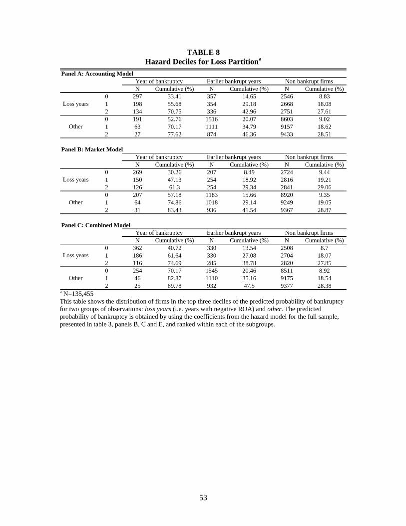
53

TABLE 8

Hazard Deciles for Loss Partitiona

Panel A: Accounting Model

Year of bankruptcy Earlier bankrupt years Non bankrupt firms

N Cumulative (%) N Cumulative (%) N Cumulative (%)

0 297 33.41 357 14.65 2546 8.83

1 198 55.68 354 29.18 2668 18.08

2 134 70.75 336 42.96 2751 27.61

0 191 52.76 1516 20.07 8603 9.02

1 63 70.17 1111 34.79 9157 18.62

2 27 77.62 874 46.36 9433 28.51

Panel B: Market Model

Year of bankruptcy Earlier bankrupt years Non bankrupt firms

N Cumulative (%) N Cumulative (%) N Cumulative (%)

0 269 30.26 207 8.49 2724 9.44

1 150 47.13 254 18.92 2816 19.21

2 126 61.3 254 29.34 2841 29.06

0 207 57.18 1183 15.66 8920 9.35

1 64 74.86 1018 29.14 9249 19.05

2 31 83.43 936 41.54 9367 28.87

Panel C: Combined Model

Year of bankruptcy Earlier bankrupt years Non bankrupt firms

N Cumulative (%) N Cumulative (%) N Cumulative (%)

0 362 40.72 330 13.54 2508 8.7

1 186 61.64 330 27.08 2704 18.07

2 116 74.69 285 38.78 2820 27.85

0 254 70.17 1545 20.46 8511 8.92

1 46 82.87 1110 35.16 9175 18.54

2 25 89.78 932 47.5 9377 28.38

Loss years

Other

Loss years

Other

Loss years

Other

a N=135,455

This table shows the distribution of firms in the top three deciles of the predicted probability of bankruptcy

for two groups of observations: loss years (i.e. years with negative ROA) and other. The predicted

probability of bankruptcy is obtained by using the coefficients from the hazard model for the full sample,

presented in table 3, panels B, C and E, and ranked within each of the subgroups.

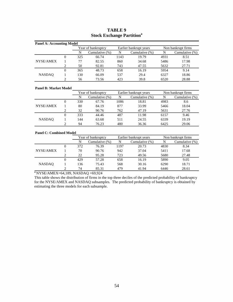
54

TABLE 9

Stock Exchange Partitiona

Panel A: Accounting Model

Year of bankruptcy Earlier bankrupt years Non bankrupt firms

N Cumulative (%) N Cumulative (%) N Cumulative (%)

0 325 66.74 1143 19.79 4931 8.51

1 77 82.55 860 34.68 5486 17.98

2 50 92.81 743 47.55 5632 27.71

0 365 48.73 658 16.19 5954 9.14

1 130 66.09 537 29.4 6327 18.86

2 56 73.56 423 39.8 6520 28.88

Panel B: Market Model

Year of bankruptcy Earlier bankrupt years Non bankrupt firms

N Cumulative (%) N Cumulative (%) N Cumulative (%)

0 330 67.76 1086 18.81 4983 8.6

1 80 84.19 877 33.99 5466 18.04

2 32 90.76 762 47.19 5631 27.76

0 333 44.46 487 11.98 6157 9.46

1 144 63.68 511 24.55 6339 19.19

2 94 76.23 480 36.36 6425 29.06

Panel C: Combined Model

Year of bankruptcy Earlier bankrupt years Non bankrupt firms

N Cumulative (%) N Cumulative (%) N Cumulative (%)

0 372 76.39 1197 20.73 4830 8.34

1 70 90.76 942 37.04 5411 17.68

2 22 95.28 723 49.56 5680 27.48

0 429 57.28 658 16.19 5890 9.05

1 136 75.43 568 30.16 6290 18.71

2 74 85.31 479 41.94 6446 28.61

NASDAQ

NYSE/AMEX

NASDAQ

NYSE/AMEX

NASDAQ

NYSE/AMEX

a NYSE/AMEX=64,189, NASDAQ =69,924

This table shows the distribution of firms in the top three deciles of the predicted probability of bankruptcy

for the NYSE/AMEX and NASDAQ subsamples. The predicted probability of bankruptcy is obtained by

estimating the three models for each subsample.

55

TABLE 10

Time Series Regressions

Panel A: Spearman and Pearson correlation matrix

T MDREST MHIGHDCACC MHIGHRD MBTM MNROAI

T 1.0000 0.8726 0.6552 0.9741 -0.8393 0.9182

<.0001 <.0001 <.0001 <.0001 <.0001

MDREST 0.9842 1.0000 0.4256 0.8907 -0.8162 0.8009

<.0001 0.0108 <.0001 <.0001 <.0001

MHIGHDCACC 0.68459 0.68045 1 0.61181 -0.60566 0.61419

<.0001 <.0001 <.0001 0.0001 <.0001

MHIGHRD 0.9992 0.9847 0.6880 1.0000 -0.8711 0.9646

<.0001 <.0001 <.0001 <.0001 <.0001

MBTM -0.8532 -0.8369 -0.6980 -0.8552 1.0000 -0.8320

<.0001 <.0001 <.0001 <.0001 <.0001

MNROAI 0.9140 0.8990 0.6356 0.9120 -0.8132 1.0000

<.0001 <.0001 <.0001 <.0001 <.0001

Panel B: Accounting Model

(1) (2) (3) (4) (5) (6)

Intercept 1.0913 0.9104 1.0257 1.0123 0.4578 1.0008

(48.76) (53.21) (11.28) (48.37) (7.34) (49.79)

MDREST -4.7567

(-6.1)

MHIGHDCACC -0.7252

(-1.95)

MHIGHRD -0.8869

(-10.69)

MBTM 0.8998

(6.18)

MNROAI -0.6610

(-8.63)

T -0.0102

(-13.01)

R2 0.7757 0.4762 0.0897 0.7308 0.6216 0.6227

N 28 31 29 28 29 30

Panel C: Market Model

(1) (2) (3) (4) (5) (6)

Intercept 0.8458 0.8423 0.8270 0.8411 0.8276 0.8400

(30.34) (58.85) (23.12) (38.03) (21.16) (33.39)

MDREST -1.3189

(-2.79)

MHIGHDCACC 0.0041

(0.03)

MHIGHRD -0.0724

(-0.76)

MBTM -0.0082

(-0.09)

MNROAI -0.0507

(-0.57)

T -0.0007

(-0.74)

R2 -0.0171 0.0447 -0.0357 -0.0133 -0.0368 -0.0225

N 30 29 30 30 29 30

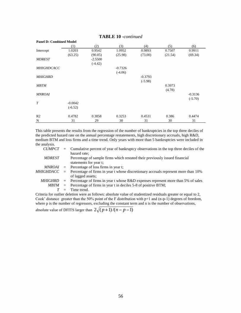
56

TABLE 10 -continued Panel D: Combined Model

(1) (2) (3) (4) (5) (6)

Intercept 1.0203 0.9542 1.0952 0.9893 0.7507 0.9911

(63.25) (90.05) (25.98) (73.00) (21.54) (69.34)

MDREST -2.5500

(-4.42)

MHIGHDCACC -0.7326

(-4.06)

MHIGHRD -0.3793

(-5.98)

MBTM 0.3973

(4.78)

MNROAI -0.3136

(-5.70)

T -0.0042

(-6.52)

R2 0.4782 0.3858 0.3253 0.4531 0.386 0.4474

N 31 29 30 31 30 31 This table presents the results from the regression of the number of bankruptcies in the top three deciles of

the predicted hazard rate on the annual percentage restatements, high discretionary accruals, high R&D,

medium BTM and loss firms and a time trend. Only years with more than 5 bankruptcies were included in

the analysis.

CUMPCT

MDREST

=

Cumulative percent of year of bankruptcy observations in the top three deciles of the

hazard rate;

Percentage of sample firms which restated their previously issued financial

statements for year t;

MNROAI = Percentage of loss firms in year t;

MHIGHDACC = Percentage of firms in year t whose discretionary accruals represent more than 10%

of lagged assets;

MHIGHRD

MBTM

=

=

Percentage of firms in year t whose R&D expenses represent more than 5% of sales

Percentage of firms in year t in deciles 5-8 of positive BTM;

T = Time trend.

Criteria for outlier deletion were as follows: absolute value of studentized residuals greater or equal to 2,

Cook’ distance greater than the 50% point of the F distribution with p+1 and (n-p-1) degrees of freedom,

where p is the number of regressors, excluding the constant term and n is the number of observations,

absolute value of DFITS larger than )1/()1(2 pnp

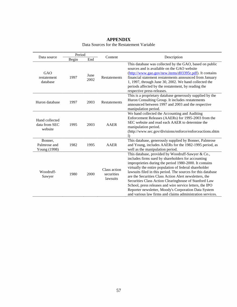
57

APPENDIX Data Sources for the Restatement Variable

Data source Period

Content Description Begin End

GAO

restatement

database

1997 June

2002 Restatements

This database was collected by the GAO, based on public

sources and is available on the GAO website

(http://www.gao.gov/new.items/d03395r.pdf). It contains

financial statement restatements announced from January

1, 1997, through June 30, 2002. We hand collected the

periods affected by the restatement, by reading the

respective press-releases.

Huron database 1997 2003 Restatements

This is a proprietary database generously supplied by the

Huron Consulting Group. It includes restatements

announced between 1997 and 2003 and the respective

manipulation period.

Hand collected

data from SEC

website

1995 2003 AAER

We hand collected the Accounting and Auditing

Enforcement Releases (AAERs) for 1995-2003 from the

SEC website and read each AAER to determine the

manipulation period.

(http://www.sec.gov/divisions/enforce/enforceactions.shtm

l)

Bonner,

Palmrose and

Young (1998)

1982 1995 AAER

This database, generously supplied by Bonner, Palmrose

and Young, includes AAERs for the 1982-1995 period, as

well as the manipulation period.

Woodruff-

Sawyer 1980 2000

Class action

securities

lawsuits

This database, provided by Woodruff-Sawyer & Co.,

includes firms sued by shareholders for accounting

improprieties during the period 1980-2000. It contains

virtually the entire population of federal shareholder

lawsuits filed in this period. The sources for this database

are the Securities Class Action Alert newsletters, the

Securities Class Action Clearinghouse of Stanford Law

School, press releases and wire service letters, the IPO

Reporter newsletter, Moody's Corporation Data System

and various law firms and claims administration services.