robust voice activity detection using long-term signal ...ict.usc.edu/pubs/robust voice activity...

Robust voice activity detection using long-term signal

variability1

Prasanta Kumar Ghosh⋆, Andreas Tsiartas and Shrikanth Narayanan

Signal Analysis and Interpretation Laboratory, Department of Electrical Engineering,

University of Southern California, Los Angeles, CA 90089

[email protected], [email protected], [email protected]

Ph: (213) 821-2433, Fax: (213) 740-4651

Abstract: We propose a novel long-term signal variability (LTSV) measure, which describes

the degree of non-stationarity of the signal. We analyze the LTSV measure both analytically and

empirically for speech and various stationary and non-stationary noises. Based on the analysis,

we find that the LTSV measure can be used to discriminate noise from noisy speech signal

and, hence, can be used as a potential feature for voice activity detection (VAD). We describe

an LTSV-based VAD scheme and evaluate its performance under eleven types of noises and

five types of signal-to-noise ratio (SNR) conditions. Comparison with standard VAD schemes

demonstrates that the accuracy of the LTSV-based VAD scheme averaged over all noises and

all SNRs is ∼6% (absolute) better than that obtained by the best among the considered VAD

schemes, namely AMR-VAD2. We also find that, at -10dB SNR, the accuracies of VAD obtained

by the proposed LTSV-based scheme and the best considered VAD scheme are 88.49% and

79.30% respectively. This improvement in the VAD accuracy indicates the robustness of the

LTSV feature for VAD at low SNR condition for most of the noises considered.

EDICS: SPE-ROBU

1Copyright (c) 2010 IEEE. Personal use of this material is permitted. However, permission to use this materialfor any other purposes must be obtained from the IEEE by sending a request to [email protected].

1

1 Introduction

Voice activity detection (VAD) refers to the problem of distinguishing speech from non-speech

regions (segments) in an audio stream. The non-speech regions could include silence, noise, or a

variety of other acoustic signals. VAD is challenging in low signal-to-noise ratio (SNR), especially

in non-stationary noise, because both low SNR and a non-stationary noisy environment tend to

cause significant detection errors. There is a wide range of applications for VAD, including mobile

communication services [1], real-time speech transmission on the Internet [2], noise reduction for

digital hearing aid devices [3], automatic speech recognition [4], and variable rate speech coding

[5].

Being a critical component in many applications, VAD has had a lot of attention in the

research community over the last few decades. Researchers have proposed a variety of features

exploiting the spectro-temporal properties of speech and noise to detect the speech segments

present in a noisy observed signal. Many existing algorithms for VAD use features that depend

on energy [6, 7, 8]. Some algorithms use a combination of zero-crossing rate (ZCR) and energy

[9]; others have used correlation coefficients [10], the wavelet transform coefficients [11], Walsh

basis function representation [12], and a distance measure of the cepstral features [13]. More

complex algorithms use more than one feature to detect speech [7, 14]. Among the various

other proposed features, negentropy has been shown to be robust for VAD [15, 16] at low SNR.

Negentropy is the entropy computed using the probability density function (pdf) obtained from

normalized short-time spectrum. All of the above-mentioned features are typically computed

from the signal along short-term analysis frames (usually 20 msec long), based on which VAD

decisions are taken at each frame. In contrast to the use of frame level features, Ramirez et

al [23] proposed the use of long-term spectral divergence between speech and noise for VAD,

although they assign the VAD decision directly to the frame in the middle of the chosen long

analysis window. Also, the long-term feature proposed in [23] requires average noise spectrum

2

magnitude information, which might not be accurately available in practice. In general, no

particular feature or specific set of features has been shown to perform uniformly well under

different noise conditions. For example, energy-based features do not work well in low SNR

[22] and similarly, under colored noise, negentropy fails to distinguish speech regions from noise

with good accuracy due to the colored spectrum of speech. Also, SNR estimation is a critical

component in many of the existing VAD schemes, which is particularly difficult in non-stationary

noise [24]. Thus, the VAD problem still remains challenging and requires the design of further

robust features and algorithms.

Recent works on VAD have been mostly statistical model based [17, 18, 19, 20]. In this

approach, VAD is posed as a hypothesis testing problem with statistical models of speech and

noise, although assumptions made about the statistics of noise [17, 18, 19, 20] do not always hold

in practice. In the short-term frame-level analysis framework, this hypothesis testing problem

can be stated as follows: given a frame of observed signal {x(n)}Nw−1n=0 (Nw is the frame duration

in number of samples), the goal is to determine whether the given frame belongs to only noise

(H0 : x(n) = N(n)) or noisy speech (H1 : x(n) = s(n) + N(n)). s(n) and N(n) denote

the samples of speech and noise respectively. To check the robustness of both feature-based

and model-based approaches, the corresponding VAD performances should be evaluated on a

wide range of noises (stationary, non-stationary, impulsive) and under different SNR conditions

(particularly at low SNR such as -10dB or -5dB).

Signal characteristics of speech and non-speech sounds have different variability profiles. This

can be advantageously used to discriminate them. For example, a person with average speaking

rate produces approximately 10-15 phonemes per second [21]. These phonemes have different

spectral characteristics. Due to this variability in signal characteristics over time, the speech

signal is non-stationary. On the other hand, ideally there is no change over time in the statistics

of the stationary noises (both white and colored). The signal characteristics of non-stationary

noises change with time; however, we need a metric to compare the variability of non-stationary

3

noise with that of speech. For computing such a metric, we need to analyze the signal over

longer duration in contrast to the usual short-term analysis.

In this work, we have proposed a novel long-term signal variability (LTSV) measure, by

which the degree of non-stationarity in various signals can be compared. We have demonstrated

the usefulness of the LTSV measure as a feature for VAD and have experimentally evaluated

its performance under a variety of noise types and SNR conditions (eleven noise types including

white, pink, tank, military vehicle, jet cockpit, HF channel, F16 cockpit, car interior, machine

gun, babble, and factory noise in five different SNR conditions: -10dB, -5dB, 0dB, 5dB and

10dB). For the proposed signal variability measure, the analysis window goes beyond the usual

short-term frame size. The short-term analysis assumes that the speech signal is slowly varying

and stationary over 20 msec. The rationale behind our choice of a long analysis window is

to obtain a realistic measure of non-stationarity or variability in signal characteristics, which

cannot be captured with a short window of 20 msec. We hypothesize that the proposed long-

term variability measure for speech will be distinctly greater compared to that obtained for

commonly encountered noises. We theoretically show that in additive stationary noise, even at

low SNR, it is possible to distinguish speech regions from stationary noisy regions using our

proposed method, which is not possible using short-time energy-based features [22]. Energy-

based features depend on the signal amplitude and hence change when the signal is scaled, but

our feature is based on the degree of non-stationarity of the signal, which does not get affected by

scaling the signal. For additive non-stationary noises, we show experimentally that it is possible

to distinguish speech from non-stationary noise with an accuracy as good as that for stationary

noise, unless the non-stationary noise and speech have a similar degree of variability, measured

by the proposed LTSV metric.

From the LTSV measure, we obtain an indication whether there is a speech signal in the

respective long analysis window. However, this decision is not assigned to a 10-20 msec frame in

the middle of the long window, unlike [23], for example. We repeat the analysis process across

4

the signal stream with a small shift (this shift determines how coarse we want to make VAD).

Thus, we obtain decisions over long windows for each shift. We assimilate all these decisions to

arrive at the final frame-level VAD decision. We find that, by utilizing signal information over

a longer window, we can make VAD more robust even at low SNR.

2 Long-term signal variability measure

The long-term signal variability (LTSV) measure at any time is computed using the last R

frames of the observed signal x(n) with respect to the current frame of interest. The LTSV,

Lx(m), at the mth (m ∈ Z) frame is computed as follows:

Lx(m)△=

1

K

K∑

k=1

(

ξxk (m) − ξx(m)

)2(1)

where, ξx(m) =1

K

K∑

k=1

ξxk (m)

and ξxk (m)

△= −

m∑

n=m−R+1

Sx(n, ωk)∑m

l=m−R+1 Sx(l, ωk)log

(

Sx(n, ωk)∑m

l=m−R+1 Sx(l, ωk)

)

. (2)

Sx(n, ωk) is the short time spectrum at ωk. It is computed as

Sx(n, ωk) = |X(n, ωk)|2 , where X(n, ωk) =

Nw+(n−1)Nsh∑

l=(n−1)Nsh+1

w(l − (n − 1)Nsh − 1)x(l)e−jωkl, (3)

w(i), 0 ≤ i < Nw is the short-time window, Nw is the frame length, and Nsh is the frame shift

duration in number of samples. X(n, ωk) is the short-time Fourier transform (STFT) coefficient

at frequency ωk, computed for the nth frame.

ξxk (m) is essentially an entropy measure on the normalized short-time spectrum computed

at frequency ωk over R consecutive frames, ending at the mth frame. The signal variability

measure Lx(m) is the sample variance of {ξxk (m)}K

k=1, i.e., the sample variance of entropies

computed at K frequency values. Lx(m) is, therefore, dependent on the choice of K frequency

5

values {ωk}Kk=1, R, and K itself.

Note that Lx(m) is invariant to amplitude scaling of the observed signal x(n). Lx(m) is

significantly greater than zero only when the entropies {ξxk(m)}K

k=1 computed at K frequencies

are significantly different from each other. Lx(m)=0 if {ξxk(m)}K

k=1 are identical for all k =

1, ...,K.

2.1 Stationary noise case

Let x(n) be a stationary noise (need not be white) N(n). Since N(n) is stationary, the ideal

noise spectrum does not change with time, i.e., SN (n, ωk) is ideally constant for all n. Let us

assume the actual spectrum of noise is known and SN (n, ωk) = σk, ∀n. Thus, using eqn. (2),

ξNk (m) = log R, ∀k2 and, hence, using eqn. (1) LN (m)=0.

Now consider x(n) to be speech in additive stationary noise, i.e., x(n) = S(n) + N(n). This

means that, ideally, Sx(n, ωk) = SS(n, ωk)+σk (assuming noise is uncorrelated to signal), where

SS(n, ωk) is the actual speech spectrum. Thus,

ξS+Nk (m) = −

m∑

n=m−R+1

SS(n, ωk) + σk∑m

l=m−R+1 SS(l, ωk) + Rσk

log

(



)

(4)

Note that log R = ξNk (m) ≥ ξS+N

k (m) ≥ ξSk (m) ≥ 0, where ξS

k (m) is the entropy measure

when x(n) is only speech S(n) (without any additive noise) and ξSk (m) can be obtained from

eqn. (4) by setting σk = 0 (see appendix A for proof). This means that if there is only speech at

frequency ωk over R consecutive frames, the entropy measure will have a smaller value compared

to that of speech plus noise; with more additive stationary noise, the entropy measure increases,

and it takes the maximum value when there is no speech component (only noise) at frequency ωk

over R frames. This means that the proportion of the energies of speech and noise (SNR) plays

an important role in determining how large or small the entropy measure ξS+Nk (m) is going to

be. Let us denote the SNR at frequency ωk at nth frame by SNRk(n)

(

△= SS(n,ωk)

σk

)

. It is easy

2Note that ξx

k (m) being an entropy measure can take a maximum value of log R, for a fixed choice of R.

6

to show that eqn. (4) can be rewritten as follows:

ξS+Nk (m) =

∑ml=m−R+1 SNRk(l)

∑ml=m−R+1 SNRk(l) + R

ξSk (m) +

R∑m

l=m−R+1 SNRk(l) + RξNk (m)

−m∑

n=m−R+1

SNRk(n)∑m

l=m−R+1 SNRk(l) + Rlog

1 + 1SNRk(n)

1 + R∑

m

l=m−R+1SNRk(l)

−m∑

n=m−R+1

1∑m

l=m−R+1 SNRk(l) + Rlog

SNRk(n) + 1∑

m

l=m−R+1SNRk(l)

R+ 1

(5)

The first two terms jointly are equal to the convex combination of ξSk (m) and ξN

k (m). The third

and fourth terms are additional terms. If SNRk(n) ≫ 1, 1SNRk(n) ≈ 0, 1

SNRk(n)+R≈ 0, then the

second, third and fourth terms turn very small and, hence, negligible; thus for high SNR at ωk,

ξS+Nk (m) ≈ ξS

k (m). Similarly, for low SNR (SNRk(n) ≪ 1), ξS+Nk (m) ≈ ξN

k (m).

As LS+N(m) is an estimate of variance of{

ξS+Nk (m)

}K

k=1and ξS+N

k (m) depends on SNRk,

the value of LS+N (m) also depends on the SNRs at {ωk}Kk=1. If SNRk(m) ≪ 1, ∀k, then

ξS+Nk (m) ≈ ξN

k (m) = log R, ∀k and hence LS+N (m) ≈ 0. On the other hand, let us consider

the case where the signal contains speech with high SNR. However, it is well known that speech

is a low pass signal; the intensity of the speech component at different frequencies varies widely,

even up to a range of 50 dB[25]. Thus, in additive stationary noise, SNRk also varies widely

across frequency depending on the overall SNR. Thus, we expect LS+N(m) to be significantly

greater than zero.

Although for the sake of analysis above, we assumed the actual spectrum of noise and speech

are known, in practice, we don’t know σk for any given stationary noise. Thus, we empirically

investigate the LTSV measure when the spectrum is estimated from real signal. In this work,

we estimate both SS(n, ωk) and σk by the periodogram method [26] of spectral estimation (eqn.

(3)). Fig. 1(a) shows the histogram of log10 (LN (m)) for stationary white noise and histogram

of log10 (LS+N(m)) for speech in additive stationary white noise at 0dB SNR. For demonstrating

the histogram properties, we consider the logarithm of the LTSV feature for better visualization

in the small value range of LTSV. In this example, the number of realizations of LN and LS+N

7

are 375872 and 401201, respectively. These samples were computed at every frame from noisy

speech obtained by adding white noise to the sentences of the TIMIT training corpus [27] at 0dB

SNR. Note that the LTSV computed at the mth frame (i.e. Lx(m)) is considered to be LS+N(m)

if there are speech frames between (m − R + 1)th and mth frame. The sampling frequency for

speech signal is Fs=16kHz. The Hanning window is used as the short-time window, w(i) (as

in eqn. (3)), and we chose the following parameter values Nw=320, Nsh=Nw

2 , R=30, K=448,

and {ωk}Kk=1 uniformly distributed between 500 and 4000 Hz. As the spectrum of the noise

and the signal plus noise are both estimated using the periodogram, LN (m) is not exactly zero

(LN (m) → 0 is equivalent to log10 (LN (m)) → −∞) although LS+N (m) > 0. The periodogram

estimate of spectrum is biased and has high variance [26]. In spite of this, on average, the values

of LN (m) are closer to zero compared to that of LS+N (m); this demonstrates that the entropy

measure ξxk (m) varies more over different ωk when there is speech compared to when there is

only noise in the observed signal. As the proportion of speech and noise in the observed signal

determines LS+N(m), we can interpret the above statement in the following way: LTSV captures

how SNRk varies across K frequencies over R frames without explicitly calculating SNRs at

{ωk}Kk=1. Fig. 1(a) also shows the histogram of log10 (LS(m)). The sample mean and sample

standard deviation (SD) of the realizations of LN , LS+N , and LS are tabulated in the figure.

It is clear that in additive noise the mean LTSV decreases (from 14.16×10−2 to 6.65×10−2).

The SD of LN (1.77×10−3) is less than that of LS+N (5.46×10−2). Thus, in the presence of

speech in R frames, LTSV can take a wider range of values compared to that in the absence of

speech. We see that there is overlap between the histograms of log10 (LN ) and log10 (LS+N).

We calculated the total misclassification error among these realizations of LN and LS+N , which

is the sum of the speech detection error (this happens when there is speech over R frames, but

gets misclassified as noise) and non-speech detection error. This was done using a threshold

obtained by the equal error rate (EER) of the region operating characteristics (ROC) curve [30].

The total misclassification error turned out to be 6.58%.

8

−10 −8 −6 −4 −2 00

0.05

0.1

log10

(LTSV)

Nor

mal

ized

Cou

nt

White Noise (0dB SNR)

Noise+SpeechNoiseSpeech

−10 −8 −6 −4 −2 00

0.05

0.1

0.15

log10

(LTSV)

Nor

mal

ized

Cou

nt


(b)

(a)

Total MisClassification Error=1.53%

S 7.00x10 −2 7.47x10 −2

N 0.11x10 −3 0.05x10 −3

N+S 1.99x10 −2 2.58x10 −2

LTSV Mean SD


S 14.16x10 −2 8.39x10 −2

N+S 6.65x10 −2 5.46x10 −2

N 8.60x10 −3 1.77x10 −3

LTSV Mean SD

Figure 1: Histogram of the logarithmic LTSV (log10 (LTSV )) measure of white noise and speechin additive white noise (0dB SNR) using (a) the periodogram estimate of spectrum (b) theBartlett-Welch estimate of spectrum. The tables in the figures show the sample mean and sampleSD of the realizations of LN , LS+N , and LS.

We found that a better estimate (unbiased with low variance) of the signal spectrum and the

noise spectrum leads to a better estimate of LN (m) and LS+N(m) (see appendix B for details).

Therefore, we use the Bartlett-Welch method of spectral estimation [26]; we estimate the signal

spectrum by averaging spectral estimates of M consecutive frames. Thus, eqn. (3) is modified

to

Sx(n, ωk) =1

M

n∑

p=n−M+1

∣

∣

∣

∣

∣

∣

Nw+(p−1)Nsh∑

l=(p−1)Nsh+1

w(l − (p − 1)Nsh − 1)x(l)e−jωkl

∣

∣

∣

∣

∣

∣

2

(6)

Fig. 1(b) shows the histograms of log10 (LN(m)), log10 (LS+N (m)), and log10 (LS(m)), where

the spectral estimates are obtained by the Bartlett-Welch method (M=20). We observe that

the mean of LN has moved closer to 0 compared to that obtained using the periodogram method

in Fig. 1(a). The SD of LN has also decreased; these suggest that the estimate of LN is better

9

using the Bartlett-Welch method compared to the periodogram. The mean and SD of both

LS+N and LS have also decreased. However, since we don’t know the true values of LTSV for

speech (and speech+noise), we can’t really comment on how good the estimates of LS and LS+N

are in Fig. 1(b) compared to those of Fig. 1(a). The total misclassification error turned out to

be 1.53%. The reduction in misclassification error from 6.58% (Fig. 1(a)) to 1.53% (Fig. 1(b);

76.75% relative reduction) suggests that the estimate of Lx using the Bartlett-Welch method

improves the speech hit rate and thus is useful for VAD.

−10 −8 −6 −4 −2 00

0.05

0.1

log10

(LTSV)

Nor

mal

ized

Cou

nt

Pink Noise (0dB SNR)


−10 −8 −6 −4 −2 00

0.05

0.1

0.15

log10

(LTSV)

Nor

mal

ized

Cou

nt


(a)

(b)Total MisClassification Error=1.14%

N+S 2.09x10 −2 2.57x10 −2

N 0.12x10 −3 0.06x10 −3

S 7.00x10 −2 7.49x10 −2

LTSV Mean SD


LTSV Mean SD

N+S 7.45x10 −2 5.73x10 −2

N 8.60x10 −3 1.60x10 −3

S 14.16x10 −2 8.39x10 −2

Figure 2: Histogram of the logarithmic LTSV (log10 (LTSV )) measure of pink noise and speechin additive pink noise (0dB SNR) using (a) the periodogram estimate of spectrum (b) the Bartlett-Welch estimate of spectrum. The tables in the figures show the sample mean and sample SD ofthe realizations of LN , LS+N , and LS.

Fig. 2 repeats Fig. 1 for stationary pink noise. We observe similar trends from Fig. 2(a) to

Fig. 2(b) as seen from Fig. 1(a) to Fig. 1(b). Since pink noise is colored, LS+N(m) for pink

noise is not the same as that of white noise. However, for both white and pink noises, the mean

of LN using the periodogram method is of the order of 10-2 and that using the Barlett-Welch

method is of the order of 10−4. Thus, on average, LN obtained by the Bartlett-Welch method is

10

closer to its theoretical value (0) compared to that obtained by the periodogram method. The

misclassification error for additive pink noise reduces from 4.86% for the periodogram method

to 1.14% (76.54% relative reduction) for the Bartlett-Welch method. This suggests that the

temporal averaging of the short-time spectrum is appropriate to make the estimate of LTSV

more robust for VAD in the case of stationary noise even when it is colored.

2.2 Nonstationary noise case

The spectrum of nonstationary noise varies with time. Thus, when x(n) is a nonstationary

noise, Lx(m) is no longer 0 even when the actual spectrum of the signal is known and used to

compute Lx(m). Lx(m) depends on the type of noise and its degree of non-stationarity and

hence becomes analytically intractable in general. Speech is a non-stationary signal. Thus,

speech in additive nonstationary noise makes the analysis even more challenging. However, the

following observations can be made about Lx(m) when noise is nonstationary:

• ξxk (m) depends on how rapidly Sx(n, ωk) changes with n, and Lx(m) depends on how

different ξxk (m), k = 1, ...,K are.

• If Sx(n, ωk) is slowly varying with n for all {ωk}Kk=1, ξx

k (m) is expected to be higher for all

{ωk}Kk=1 and hence, Lx(m) will be close to 0.

• Similarly, if Sx(n, ωk) varies rapidly over n for all {ωk}Kk=1, ξx

k (m) becomes small ∀k and

hence Lx(m) will also be close to 0.

• However, if Sx(n, ωk) varies with n slowly at some ωk and largely at some other ωk, Lx(m)

would tend to take a high value. When x(n) = S(n)+N(n), how Sx(n, ωk) varies with ωk

depends on the SNRk.

For nonstationary noises, we demonstrate the efficacy of the LTSV measure by simula-

tions. We obtained samples of non-stationary noises, namely tank, military vehicle, jet cockpit,

11

HFchannel, F16 cockpit, car interior, machine gun, babble, and factory noise from the NOISEX-

92 database [28]. We added these noise samples to the sentences of the TIMIT training corpus

[27] at 0dB SNR to compute realizations of LN , LS+N , and LS . For illustrations, Fig. 3 (a) and

(b) show the histograms of log10 (LN ), log10 (LS+N), and log10 (LS) using the Bartlett-Welch

spectral estimates for additive (0dB) car interior noise and jet cockpit noise, respectively. The

parameter values for Fig. 3 are chosen to be the same as those used for Fig. 1.

−10 −8 −6 −4 −2 00

0.05

0.1

log10

(LTSV)

Nor

mal

ized

Cou

nt

Car interior Noise (0dB SNR)


−10 −8 −6 −4 −2 00

0.05

0.1

log10

(LTSV)

Nor

mal

ized

Cou

nt

Jet cockpit Noise (0dB SNR)


(a)

(b)


LTSV Mean SD


LTSV Mean SD

N+S 6.85x10 −2 7.24x10 −2

N 0.17x10 −3 0.11x10 −3

S 7.00x10 −2 7.47x10 −2

N+S 1.77x10 −2 1.73x10 −2

N 0.18x10 −3 0.12x10 −3

S 7.00x10 −2 7.47x10 −2

Figure 3: Histogram of the logarithmic LTSV (log10 (LTSV )) measure using the Bartlett-Welchspectral estimates for (a) car interior noise and speech in additive car interior noise (0dB), and(b) jet cockpit noise and speech in additive jet cockpit noise (0dB). The tables in the figures showthe sample mean and sample SD of the realizations of LN , LS+N , and LS.

In Fig. 3(a) (car interior noise), it is seen that the histogram of log10 (LS+N) is not much

different from that of log10 (LS). This means that in additive car interior noise the LTSV measure

of noisy speech does not change significantly compared to that of speech only. Computation of

SNRk at {ωk}Kk=1 for additive car noise (at 0dB SNR) reveals that the average SNRk is 15dB

in the range of frequencies between 500 and 4000 Hz. The spectrum of car interior noise has

a relatively large low-pass component below 500 Hz. {SNRk}Kk=1 being high, LS and LS+N

12

are similar. From Fig. 3 (a) it can also be seen that the mean of LN is approximately 500

times smaller than the mean of LS+N and, also, the overlap between the histograms of LN

and LS+N is negligible, resulting in a very small misclassification error of 0.04%. Similar to

the case of stationary white and pink noises, the use of the Bartlett-Welch method for spectral

estimation provides a 63.63% relative reduction in misclassification error compared to that of the

periodogram method (0.11%) in additive car noise. Similarly, the misclassification error reduces

from 18.11% (the periodogram method) to 1.93% (89.34% relative reduction) (the Bartlett-Welch

method) for additive jet cockpit noise.

For a comprehensive analysis and understanding, the total misclassification errors for both

stationary and non-stationary noises are presented in Table 1 using both the periodogram and

the Bartlett-Welch methods. Noises are added to speech at 0dB SNR, and M is chosen to be

20 for the Bartlett-Welch method for this experiment.

Noise Total Misclassification ErrorType Periodogram Bartlett-Welch Relative reduction

White 6.58 1.53 76.44%

Pink 4.86 1.14 76.54%

Tank 0.88 0.68 22.72%

Military Vehicle 0.27 0.22 18.51%

Jet Cockpit 18.11 1.93 89.34%

HFchannel 3.67 1.9 48.22%

F16 2.93 0.9 69.28%

Factory 1.88 2.23 -18.61%

Car 0.11 0.04 63.63%

Machine Gun 40.64 34.6 14.86%

Babble 14.56 18.59 -27.67%

Table 1: Total misclassification errors (in percent) for using the periodogram and the Bartlett-Welch method (M=20) in estimating LTSV measure. R is chosen to be 30.

Except for the case of factory and babble noise in Table 1, we observe a consistent reduction

in misclassification error when LTSV is computed using the Bartlett-Welch method (M=20)

compared to that using the periodogram method. The percentages of relative reduction indicate

that the temporal smoothing with a fixed M in the Bartlett-Welch estimate does not consistently

reduce the total misclassification error for all noises compared to that obtained by periodogram

13

estimate.

−9 −8 −7 −6 −5 −4 −3 −2 −1 00

0.05

0.1

log10

(LTSV)

Nor

mal

ized

Cou

nt

Machinegun Noise (0dB SNR)


−7 −6 −5 −4 −3 −2 −1 00

0.05

0.1

log10

(LTSV)

Nor

mal

ized

Cou

nt

Speech Babble Noise (0dB SNR)


(a)

(b)


S 7.00x10 −2 7.47x10 −2

N 3.45x10 −2 9.21x10 −2

N+S 6.36x10 −2 6.74x10 −2

LTSV Mean SD


S 7.00x10 −2 7.47x10 −2

N 6.10x10 −3 6.00x10 −3

N+S 3.16x10 −2 3.47x10 −2

LTSV Mean SD

Figure 4: Histogram of the logarithmic LTSV (log10 (LTSV )) measure using the Bartlett-Welchspectral estimates for (a) machine gun noise and speech in additive machine gun noise (0dB),and (b) babble noise and speech in additive babble noise (0dB). The tables in the figures showthe sample mean and sample SD of the realizations of LN , LS+N , and LS.

In particular, the misclassification error is high for machine gun and speech babble noise using

both the periodogram and the Bartlett-Welch method. The LTSV measure cannot distinguish

these two noises from the corresponding noisy speech. For machine gun noise, the histogram of

log10 (LN ) shows a bimodal nature (Fig. 4(a)) when the Bartlett-Welch method is used. This is

due to the fact that machine-gun noise is composed of mainly two different signals - the sound

of the gun firing and the silence in between firing. When R consecutive frames belong to silence

they yield a very small value of LN but, when R frames include portions of the impulsive sound

of firing (nonstationary event), the value of LN becomes high. This creates a hump in the

histogram exactly where the main hump of the histogram of LS+N is (Fig. 4(a)). This causes

a considerable amount of misclassification error.

14

A similar observation can be made for the case of speech babble noise. As the noise is

speech-like, it is nonstationary and causes similar values of LN and LS+N , resulting in significant

overlap between the histograms of log10 (LN ) and log10 (LS+N) (Fig. 4(b)). Due to this, a large

misclassification error is obtained.

From the simulations of non-stationary noise cases, we found that the mean LTSV of the

non-stationary noise is higher than that of stationary noise. Except for machine gun noise,

the mean LTSV of all noises is lower than that of speech. Thus, the LTSV measure reflects

the degree of non-stationarity or variability in the signal, and the signal variability in speech

is more than that in all noises considered here, except machine gun noise. When the degree of

non-stationarity of noise is similar to that of noisy speech as measured by LTSV, noise and noisy

speech can not be distinguished effectively. This happens for machine gun and babble noise,

resulting in high misclassification errors (Table 1).

3 Selection of {ωk}Kk=1, R and M

3.1 Selection of {ωk}K

k=1

From the analysis of LTSV for different noises, we realize that the higher the SNR, the better the

separation between the histograms of LS+N and LN . Thus, for a better discrimination between

LS+N and LN , we need to select the frequency values {ωk}Kk=1, for which SNRk is high enough.

Computation of SNRk for various noises reveals that SNRk is high for frequency values below

4kHz. This is particularly because speech in general is a low pass signal. It is also known that

the 500Hz to 4kHz frequency range is crucial for speech intelligibility [29]. Hence we decided to

choose ωk in this range. The exact values of {ωk}Kk=1 are determined by the sampling frequency

Fs and the order NDFT of discrete Fourier transform (DFT), used to compute the spectral

estimate of the observed signal. Thus K = NDFT

(

4000−500Fs

)

. For example, NDFT = 2048 and

FS = 16000 yield K = 448; {ωk}448k=1 are uniformly distributed between 500Hz and 4kHz.

15

3.2 Selection of R and M

R and M are parameters used for computing Lx(m) (see eqn. (6) and (2)). Our goal is to

choose R and M such that the histograms of LN and LS+N are maximally discriminative since

the better the discrimination between LN and LS+N , the better the final VAD decision. We

computed the total misclassification error (sum of two types of detection errors) as a measure of

discrimination between the histograms of LN and LS+N for given values of R and M denoted

by:

M(R,M) = Speech Detection Error + Noise Detection Error

We used receiver operating characteristics (ROC) [30] to compute M(R,M). ROC curve is a

plot of speech detection error and non-speech detection error for varying threshold γ, above which

the LTSV measure indicates speech. We chose M(R,M) and the corresponding threshold for

which two types of detection errors are equal, which is known as equal error rate (EER). Eleven

different types of noises (as mentioned in Table 1) were added to TIMIT training sentences

to generate realizations of LS+N . LN were also computed for all these different noises. The

Hanning window is used as the short-time window, w(i) (as in eqn. (6)), and we chose the

following parameter values Nw=320 (corresponds to 20 msec), Nsh=Nw

2 , K=448 and {ωk}Kk=1

uniformly distributed between 500 and 4000 Hz (as determined in section 3.1). M(R,M) are

computed for R=5, 10, 20, 30, 40, 50 (corresponding to 50 msec to 500 msec) and M=1, 5, 10,

20, 30 (corresponding to 10 msec to 300 msec). This experiment was systematically performed

for 11 types of noises and 5 different SNR conditions, i.e., -10dB, -5dB, 0dB, 5dB, 10dB. The

misclassification errors for all combinations of R and M are shown in Fig. 5 using gray valued

representation. The darker the box, the lower the value of M(R,M). Rows in Fig. 5 correspond

to different noise types and columns correspond to different SNRs (as mentioned at the top of

the columns). Except for machine gun noise, it was found that for any choice of M , M(R,M)

monotonically decreases with increasing R. However, above R=30 the reduction in M(R,M)

16

−10dB −5dB 0dB 5dB 10dB

(a)

(b)

(c)

(d)

(e)

(f)

(g)

(h)

(i)

(j)

(k)

M15102030

R 5 10 20 30 40 50 R 5 10 20 30 40 50

M15102030

M15102030

R 5 10 20 30 40 50

M15102030

R 5 10 20 30 40 50

Figure 5: Gray valued representation of M(R,M) for R=5, 10, 20, 30, 40, 50 and M=1, 5,10, 20, 30. Darker box indicates lower value: (a) white, (b) pink, (c) tank, (d) military vehicle,(e) jet cockpit, (f) HFchannel, (g) F16 cockpit, (h) factory, (i) car, (j) machine gun, (l) babblenoise.

is not significant for most of the noises (which can be seen from insignificant changes in gray

values in Fig. 5). Also a larger R leads to a larger delay in VAD decision. Hence, we restrict

possible values of R up to 30 frames i.e., R=5, 10, 20, 30. We report the combination of R and

M corresponding to the minimum value of M(R,M) in Table 2.

We observe that, except for machine gun noise, the best choice of R is 30 (which means

that the LTSV is computed over 0.3 sec). For machine gun noise, the best choices of R and

M both are found to be 10 frames (0.1 sec) for all SNR conditions. Machinegun noise consists

of two types of sounds, namely, gun-shot and silence between gun-shots. For a high value

17

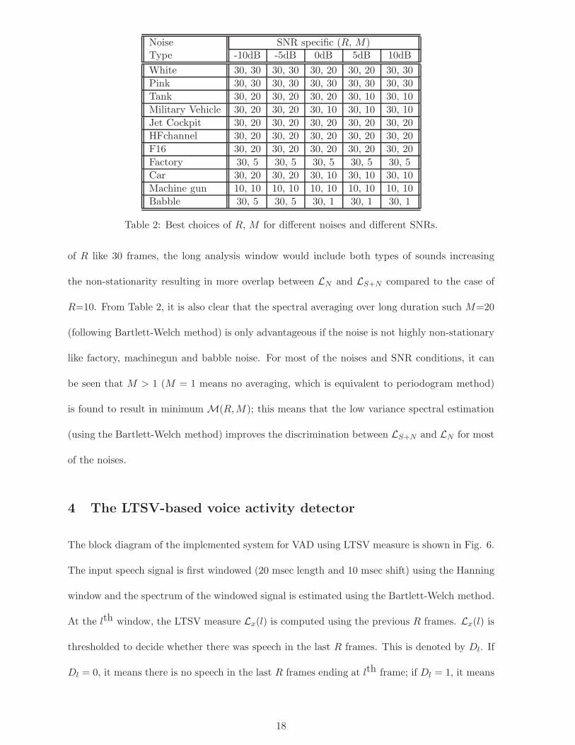
Noise SNR specific (R, M)Type -10dB -5dB 0dB 5dB 10dB

White 30, 30 30, 30 30, 20 30, 20 30, 30

Pink 30, 30 30, 30 30, 30 30, 30 30, 30

Tank 30, 20 30, 20 30, 20 30, 10 30, 10

Military Vehicle 30, 20 30, 20 30, 10 30, 10 30, 10

Jet Cockpit 30, 20 30, 20 30, 20 30, 20 30, 20

HFchannel 30, 20 30, 20 30, 20 30, 20 30, 20

F16 30, 20 30, 20 30, 20 30, 20 30, 20

Factory 30, 5 30, 5 30, 5 30, 5 30, 5

Car 30, 20 30, 20 30, 10 30, 10 30, 10

Machine gun 10, 10 10, 10 10, 10 10, 10 10, 10

Babble 30, 5 30, 5 30, 1 30, 1 30, 1

Table 2: Best choices of R, M for different noises and different SNRs.

of R like 30 frames, the long analysis window would include both types of sounds increasing

the non-stationarity resulting in more overlap between LN and LS+N compared to the case of

R=10. From Table 2, it is also clear that the spectral averaging over long duration such M=20

(following Bartlett-Welch method) is only advantageous if the noise is not highly non-stationary

like factory, machinegun and babble noise. For most of the noises and SNR conditions, it can

be seen that M > 1 (M = 1 means no averaging, which is equivalent to periodogram method)

is found to result in minimum M(R,M); this means that the low variance spectral estimation

(using the Bartlett-Welch method) improves the discrimination between LS+N and LN for most

of the noises.

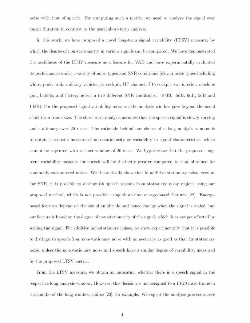
4 The LTSV-based voice activity detector

The block diagram of the implemented system for VAD using LTSV measure is shown in Fig. 6.

The input speech signal is first windowed (20 msec length and 10 msec shift) using the Hanning

window and the spectrum of the windowed signal is estimated using the Bartlett-Welch method.

At the lth window, the LTSV measure Lx(l) is computed using the previous R frames. Lx(l) is

thresholded to decide whether there was speech in the last R frames. This is denoted by Dl. If

Dl = 0, it means there is no speech in the last R frames ending at lth frame; if Dl = 1, it means

18

Compute

Lx(l)WelchMethod

Bartlett

VotingLx(l) > γ

Threshold

Update

VAD

γ

Long Term

Decisions

xl(n) Sx(l, ω)

n

x(n) windowing

Figure 6: Block diagram of the LTSV-based VAD system

Target10 msecfor VAD

R frames

R frames

R frames

R frames

l-2 l-1 l l+1 l+2

Dl

Dl+1

Dl+R

Dl+R+1

Figure 7: Long windows for voting on a 10 msec interval.

there is speech over the last R frames ending at lth frame. However, the final VAD decision is

made on every 10 msec interval by using a voting scheme3 as shown in Fig. 7. To take a VAD

decision on a target 10 msec interval indexed by l, (R+1) decisions Dl, Dl+1, ...,Dl+R+1 are first

collected on the long windows, which overlap with the target 10 msec interval. If c% of these

decisions are speech, the target 10 msec interval is marked as speech; otherwise it is marked as

noise. Experiments on the TIMIT training set shows that a high value of c leads to higher VAD

3As an alternative to the voting scheme, we also modeled the observed noisy speech as a sequence of segments(each of duration .3 sec with 50% overlap) which are either speech or silence or speech-silence boundary orsilence-speech boundary. The probability of transition from one type of segment to another is learned from thetraining data and used to decode best segment sequence given the LTSV measure for each segment. However, theperformance was not significantly improved compared to the voting scheme for all noises.

19

accuracy at 10dB SNR, while a low value of c leads to higher VAD accuracy at -10dB SNR. In

our experiment, we chose c=80, which provided the maximum VAD accuracy at 0dB SNR.

Noise and SNR specific best choices of R, M , and threshold γ were obtained in section 3.2.

However, to deploy the VAD scheme in practice, we need to update these parameters on the

fly according to the type of noise. For our current implementation, we have fixed R=30 and

M=20, since most of the noises turn out to have minimum misclassification errors for this choice

of R and M (Table 2). However, a fixed value of γ does not work well for all noises. Hence, we

designed an adaptive threshold selection scheme. γ is the threshold for LTSV measure between

two classes - noise and noisy speech. To update γ(m) at mth frame, we used two buffers BN(m)

and BS+N(m). BN (m) stored the LTSV measures of the last 100 long-windows, which were

decided as containing noise only; similarly, BS+N(m) stored the LTSV measures of the last 100

long-windows, which were decided as having speech. One hundred long-windows (with 10 msec

shift) in each buffer is equivalent to 1 sec. Since we are interested in measuring signal variability

over long duration, we assume that the degree of non-stationarity of the signal does not change

drastically over 1 sec. γ(m) is computed as the convex combination between the minimum of

the elements of BS+N(m) and maximum of the elements of BN (m) as follows:

γ(m) = αmin (BS+N (m)) + (1 − α)max (BN (m)) (7)

where α is the parameter of the convex combination4. We experimentally found that α = 0.3

results in maximum accuracy in VAD decisions over the TIMIT training set. To initialize γ,

when the LTSV-based VAD scheme starts operating, we proceed in the following way:

We assume that the initial 1 second of the observed signal x(n) is noise only. From this

1 second of x(n), we obtain 100 realizations of LN . Let µN and σ2N be the sample mean and

sample variance of these 100 realizations of LN . We initialize γ = µN + pσN , where p is selected

4As an alternative, we also performed experiments by convex combination of the average of BS+N(m) andBN (m), but the performance of VAD decisions was worse compared to that obtained by using eqn. (7).

20

0 2 4 6

10−5

LTSVγ

0 2 4 60

0.5

1

time (in sec)

VAD

0 2 4 6−1

0

1

0 2 4 6−1

0

1WHITE NOISE

0 2 4 6

10−5

LTSVγ

0 2 4 60

0.5

1

time (in sec)

VAD

0 2 4 6−1

0

1

0 2 4 6−1

0

1TANK NOISE

0 2 4 6

10−5

LTSVγ

0 2 4 60

0.5

1

time (in sec)

VAD

0 2 4 6−1

0

1

0 2 4 6−1

0

1HFCHANNEL NOISE

(a)

(b)

(c)

(d) (h)

(g)

(f)

(e) (i)

(j)

(k)

(l)

Figure 8: Illustrative example of VAD using LTSV with adaptive threshold on a randomly chosensentence from TIMIT test set: (a): Clean speech; (b): White Noise added at -10dB SNR; (c):Lx(m), γ(m) computed on (b); (d): VAD decisions on (b); (e)-(h): (a)-(d) repeated for TankNoise; (i)-(l): (a)-(d) repeated for HFchannel Noise.

0 2 4 6

10−2

LTSVγ

0 2 4 60

0.5

1

time (in sec)

VAD

0 2 4 6−1

0

1

0 2 4 6−1

0

1BABBLE NOISE

0 2 4 6

100

LTSVγ

0 2 4 60

0.5

1

time (in sec)

VAD

0 2 4 6−1

0

1

0 2 4 6−1

0

1MACHINE GUN NOISE

0 2 4 610

−5

LTSVγ

0 2 4 60

0.5

1

time (in sec)

VAD

0 2 4 6−1

0

1

0 2 4 6−1

0

1CAR INTERIOR NOISE

(a)

(b)

(c)

(d) (h)

(g)

(f)

(e) (i)

(j)

(k)

(l)

Figure 9: Illustrative example of VAD using LTSV with adaptive threshold on a randomly chosensentence from TIMIT test set: (a): Clean speech; (b): Car Interior Noise added at -10dB SNR;(c): Lx(m), γ(m) computed on (b); (d): VAD decisions on (b); (e)-(h): (a)-(d) repeated forMachine gun Noise; (i)-(l): (a)-(d) repeated for Babble Noise.

21

from a set of {1.5, 2, 2.5, 3, 3.5, 4, 4.5} to obtain the maximum accuracy of VAD decisions on

the TIMIT training set. The best choice of p was 3. Since on average the LTSV of noisy speech

is more than that of noise only (as seen in Fig. 1-4), γ should be more than the mean LTSV of

noise (µN ). The choice of p was done to select the threshold between mean values of the LTSV

of noise and noisy speech.

Fig. 8 and 9 illustrate Lx(m), γ(m) and the VAD decisions for a randomly chosen sentence

from TIMIT test set in additive (-10dB SNR) white, tank, HFchannel, car interior, machine gun,

and babble noise. It should be noted that before adding noise samples, silence of two seconds

has been added in the beginning and at the end of the utterance. This silence padded-speech is

shown in Fig. 8 and 9 (a), (e), (i) to visually compare with the VAD decisions obtained using

LTSV and the adaptive threshold scheme for six types of noises. Each column in both Fig. 8 and

9 corresponds to one type of noise, which is mentioned on top of each column. The second row

in both figures shows the speech signal in additive noise at -10dB SNR. The third row in both

figures shows Lx(m) and γ(m). Y-axes of these plots are shown in log scale to clearly show the

variation in very small values. It can be seen that the threshold γ varies with time as computed

by eqn. (7). The respective VAD decisions for six noises are shown in the last row of both

Fig. 8 and 9. Value 1 in these plots corresponds to speech and 0 corresponds to noise. Even

at -10dB SNR, VAD decisions for additive white, car, and babble noise appear approximately

correct from Fig. 8 (d), 9 (d), and (l) respectively. For machine gun noise, many noise frames

are detected as speech. For tank and HFchannel noise also, a few noise frames are detected as

speech. However, systematic performance evaluation is required for understanding the accuracy

of VAD in various noises.

5 Evaluation and results

Evaluation of a VAD algorithm can be performed both subjectively and objectively. Subjective

evaluation is done through a listening test, in which human subjects detect VAD errors [31];

22

on the other hand, objective evaluation is done using an objective criterion, which can be

computed numerically. However, subjective evaluation is often not sufficient to examine the

VAD performance because listening tests like ABC [31] fail to consider the effect of the false

alarm [18]. Hence, we use objective evaluation strategy to report the performance of the proposed

VAD algorithm.

We closely follow the testing strategy proposed by Freeman et al [1] and by Beritelli et al

[32], in which the labels obtained by the proposed VAD algorithm are compared against known

reference labels. This comparison is performed through five different parameters reflecting the

VAD performance:

1. CORRECT: Correct decisions made by the VAD.

2. FEC (front end clipping): Clipping due to speech being misclassified as noise in passing

from noise to speech activity.

3. MSC (mid speech clipping): Clipping due to speech misclassified as noise during an utter-

ance.

4. OVER (carry over): Noise interpreted as speech in passing from speech activity to noise

due to speech information carried over by the LTSV measure.

5. NDS (noise detected as speech): Noise interpreted as speech within a silence period.

FEC and MSC are indicators of true rejection, while NDS and OVER are indicators of false

acceptance. CORRECT parameter indicates the amount of correct decisions made. Thus all

four parameters FEC, MSC, NDS, OVER should be minimized and the CORRECT parameter

should be maximized to obtain the best overall system performance.

For VAD evaluation in this work, we used the TIMIT test corpus [27] consisting of 1680

individual speakers of eight different dialects, each speaking 10 phonetically balanced sentences.

Silence of an average duration of 2 sec was added before and after each utterance, and then

23

noise of each category was added at 5 different SNR levels (-10dB, -5dB, 0dB, 5dB, 10dB) to

all 1680 sentences. The test set for each noise and SNR thus consisted of 198.44 minutes of

noisy speech of which 62.13% was only noise. The noise samples of eleven categories were taken

from the NOISEX-92 database. The beginning and end locations of the speech portions of the

silence-padded TIMIT sentences were computed using the start time and the end time of the

sentence obtained from the TIMIT transcription. The final VAD decisions were computed for

every 10 msec interval. Thus, for reference, each 10 msec interval was tagged as speech or noise

using the beginning and end of speech. If a 10 msec interval overlapped with speech, it was

tagged as speech, and otherwise as noise.

The proposed adaptive-threshold LTSV (we denote this by LTSV-Adapt scheme) based VAD

scheme was run followed by the voting scheme to obtain VAD decisions at 10 msec frame level.

The noisy TIMIT test sentences were concatenated and presented in a contiguous manner to

the LTSV-Adapt VAD scheme so that the threshold could be adapted continuously. In order to

do a comparative analysis, the performance of the proposed LTSV-Adapt scheme was compared

against three modern standardized VAD schemes. These schemes are the ETSI AMR VADs

option 1 & 2 [33] and ITU G.729 AnnexB VAD [34]. The implementations were taken from

[35] and [36] respectively. The VAD decisions at every 10 msec obtained by the standard VAD

schemes and our proposed VAD scheme were compared to the references, and five different

parameters (CORRECT, FEC, MSC, NDS, OVER) were computed for eleven noises and five

SNRs. In addition to the performance of the LTSV-Adapt scheme, we report performance for the

case using noise and SNR specific R, M and γ (we denote this by LTSV-opt scheme), assuming

that we know the correct noise category and SNR. This was done to analyze how much the VAD

performance degrades when the noise information is not available or not estimated. However, for

comparing against standard VAD schemes, we used LTSV-Adapt scheme-based VAD decisions.

Fig. 10 shows five different scores (CORRECT, FEC, MSC, NDS, OVER), averaged over 5

SNRs for each noise, computed for AMR-VAD1, AMR-VAD2, G.729, LTSV-Adapt, and LTSV-

24

White Pink Tank Mil. Veh. JetCock. HF Ch. F16 Factory Car Machinegun Babble0

5

10

AMR−VAD1AMR−VAD2G.729LTSV−AdaptLTSV−Opt


50

100


0.5

1

1.5


10

20


20

40

60

CORRECT

FEC

MSC

NDS

OVER

Figure 10: CORRECT, FEC, MSC, NDS and OVER averaged over all SNRs for eleven noisesas obtained by five VAD schemes - AMR-VAD1, AMR-VAD2, G.729, LTSV-Adapt scheme andLTSV-opt scheme.

opt schemes. Fig. 11 shows the same result for -10dB SNR.

We observe a consistent reduction in average CORRECT score from LTSV-opt scheme to

LTSV-Adapt scheme for all noises (Fig. 10). The significant reduction happens for speech babble

(from 85.3% for LTSV-opt scheme to 80.3% for LTSV-Adapt scheme) and for machine gun noise

(from 78.0% for LTSV-opt scheme to 72.0% for LTSV-Adapt scheme). While machine gun noise

is impulsive in nature, speech babble is speech-like and, hence, the best choices of R and M for

these noises are different (see Table 2) compared to the R=30 and M=20 combination, which is

used in LTSV-Adapt scheme. This mismatch in R and M causes a significant difference in the

CORRECT score between the LTSV-opt scheme and the LTSV-Adapt scheme. A suitable noise

categorization scheme prior to LTSV-opt scheme can improve the VAD performance compared

to LTSV-Adapt scheme. From Fig. 10, it is clear that in terms of the CORRECT score,

AMR-VAD2 is the best among all three standard VAD schemes considered here. Hence, the

25

LTSV-Adapt scheme is compared with the AMR-VAD2 among three standard VAD schemes.

We see that on an average, the LTSV-Adapt scheme is better than the AMR-VAD2 in terms of

CORRECT score for white (6.89%), tank (0.86%), jet cockpit (5.02%), HFchannel (2.88%), F16

cockpit (3.86%), and machine gun (0.35%), and worse for pink (2.14%), military vehicle (2.01%),

factory (1.61%), car interior (1.73%), and babble (4.38%) noises. The percentage in the bracket

indicates the absolute CORRECT score by which one scheme is better than the other. LTSV-

Adapt scheme has a smaller MSC score compared to that of AMR-VAD2 for white (8.19%), pink

(8.52%), tank (2.57%), military vehicle (0.82%), jet cockpit (5.95%), HFchannel (5.92%), F16

cockpit (5.88%), Factory Noise (0.75%), and car interior (0.61%) and a larger MSC for machine

gun (4.52%) and babble noise (4.63%). The percentage in the bracket indicates the absolute

MSC score by which one scheme is better (has lower MSC) than the other. Thus, AMR-VAD2

has a larger MSC score compared to the LTSV-Adapt scheme for all noises except machine gun

and babble noise. This means, on an average, AMR-VAD2 loses more speech frames compared

to the LTSV-Adapt scheme. For babble noise, the CORRECT score of AMR-VAD2 is greater

than that of LTSV-Adapt scheme due to the fact that we use M=20, which is not the best

choice for speech babble as shown in Table 2. Speech babble being non-stationary noise, long

temporal smoothing does not help. The OVER score of the LTSV-Adapt scheme for additive

car interior noise is more than that of AMR-VAD2. This happens for pink, military vehicle,

factory, and babble noise, too. Higher values of OVER for these noises result in a lower value of

the CORRECT score of the LTSV-Adapt scheme compared to that of AMR-VAD2. High value

of OVER implies that noise frames at the speech-to-noise boundary are detected as speech.

Depending on the application, such errors can be tolerable compared to high MSC and high

NDS. High MSC is harmful for any application since high MSC implies that speech frames are

decided as noise frames.

It should be noted that in the LTSV-Adapt scheme, we are neither estimating the SNR of the

observed signal nor estimating the type of noise. This is an SNR independent scheme; however,

26


2

4

6

8

AMR−VAD1AMR−VAD2G.729LTSV−AdaptLTSV−Opt


50

100


1

2

3


10

20


20

40

60

CORRECT

FEC

MSC

NDS

OVER

Figure 11: CORRECT, FEC, MSC, NDS and OVER at -10dB SNR for eleven noises as obtainedby five VAD schemes - AMR-VAD1, AMR-VAD2, G.729, LTSV-Adapt scheme and LTSV-optscheme.

the LTSV-Adapt scheme performs consistently well in all SNRs. In particular, from Fig. 11, we

observe that at -10dB SNR, the LTSV-Adapt scheme has a higher CORRECT score than that

of AMR-VAD2 for white (19.88%), pink (4.43%), tank (6.95%), jet cockpit (11.6%), HFchannel

(11.36%), F16 cockpit noise (12.48%), and factory noise (0.07%) and lower for military vehicle

(1.72%), car interior (1.37%), machine gun (1.88%), and babble noise (2.76%). These are noises

where we have mismatch between the fixed R and M used for the LTSV-Adapt scheme with the

best R and M as indicated by Table 2. Also at -10dB SNR, MSC of the LTSV-Adapt scheme

is lower than that of AMR-VAD2 for white (20.7%), pink (22.01%), tank (7.73%), military

vehicle (1.16%), jet cockpit (12.02%), HFchannel (12.83%), F16 cockpit (13.23%), Factory Noise

(2.18%), car interior (0.58%), and babble noise (3.95%) and greater for machine gun (3.82%)

noise. Compared to AMR-VAD2, the LTSV-Adapt scheme has lower NDS, too. All these imply

that the LTSV-Adapt scheme has smaller speech frame loss compared to AMR-VAD2 at -10dB

27

SNR, and hence is robust in low SNR.

6 Conclusions

We presented a novel long-term signal variability (LTSV) based voice activity detection method.

Properties of this new long-term variability measure were discussed theoretically and experi-

mentally. Through extensive experiments, we show that the accuracy of the LTSV based VAD

averaged over all noises and all SNRs is 92.95% as compared to 87.18% obtained by the best

available commercial AMR-VAD2. Similarly, at -10dB SNR, the accuracies are 88.49% and

79.30% respectively, demonstrating the robustness of LTSV feature for VAD at low SNR. While

the energy-based features for VAD are affected by signal scaling, the proposed long-term vari-

ability is not. It has also been found that for non-stationary noises, which have similar LTSV

measure as that of speech, the proposed VAD scheme fails to distinguish speech from noise

with good accuracy. However, additional modules such as noise category recognition might help

improve the result by allowing for noise-specific solutions and improve the VAD performance. If

we have knowledge of the background noise in any application or if we can estimate the category

of noise and accordingly choose the R, M and γ for minimum misclassification error on the

training set, we expect to achieve the performance of LTSV-opt scheme, which is better than

that of LTSV-Adapt scheme. We also observed that the optimum choice of c varies with SNR.

Thus, adaptively changing c by estimating the SNR of the observed signal can improve the VAD

performances. Also, a choice of low value of c improves FEC score while increases OVER score

at high SNR. On the other hand, a high value of c reduces the OVER score while increases FEC

score at low SNR. Thus, the choice of c should be tuned considering the trade-off between FEC

and OVER scores. These are part of our future works.

To improve upon the LTSV measure, we have explored using mean entropy (ξx(m)) for

VAD. Theoretically, it is easy to prove that mean entropy for noise ≥ mean entropy of S+N.

But, in practice, their histograms overlap more than those of their variance. We observed that

28

the correlation between mean and variance of the LTSV feature is high (in the range of -0.6

to -0.9); hence, using mean LTSV as an additional feature, we did not obtain any significant

improvement in VAD performance. We also performed experiments with additional features like

subband energy, subband LTSV, derivatives of LTSV, and with choices of different frequency

bands. In some cases, additional features provided improvements for some noises. Thus, in

noise-specific applications, these additional features could be useful. Also, it can be seen that

we have not used the usual hangover scheme as done in frame based VAD schemes [18]. This

is because our approach inherently takes a long-term context through variability measure. So,

there is no additional need of the hangover scheme.

One advantage of using LTSV for VAD is that there is no need for explicit SNR estimation.

At the same time, it should be noted that, depending on the choice of the longer window length,

any VAD related application is expected to suffer a delay equal to the duration of the window.

Thus, a trade-off between the delay and the robustness of VAD, particularly in low SNR, should

be examined carefully before using LTSV-based VAD scheme in a specific application.

29

A Proof of log R = ξNk (m) ≥ ξS+N

k (m) ≥ ξSk (m) ≥ 0

From eqn. (4), we rewrite the following:

ξNk (m) = −

∑mn=m−R+1

σk

Rσklog

(

σk

Rσk

)

= log R [by setting SS(n, ωk) =0]

ξS+Nk (m) = −

∑mn=m−R+1

SS(n,ωk)+σk∑

m

l=m−R+1SS(l,ωk)+Rσk

log

(

SS(n,ωk)+σk∑

m


)

ξSk (m) = −

∑mn=m−R+1

SS(n,ωk)∑

m

l=m−R+1SS(l,ωk)

log

(

SS(n,ωk)∑

m

l=m−R+1SS(l,ωk)

)

[by setting σk =0]

We know that entropy is bounded by two values [37]

0 ≤ ξS+Nk (m) ≤ log R = ξN

k (m) and 0 ≤ ξSk (m) ≤ log R = ξN

k (m) (8)

We need to showξSk (m) ≤ ξS+N

k (m) (9)

Consider eqn. (2). Let us denote Sx(n,ωk)∑

m

l=m−R+1Sx(l,ωk)

= pn, n = m − R + 1, ...,m. Then

ξxk (m) = −

m∑

n=m−R+1

Sx(n, ωk)∑m

l=m−R+1 Sx(l, ωk)log

(

Sx(n, ωk)∑m


)

= −m∑

n=m−R+1

pn log pn

= H(pm−R+1, ..., pm)

= H

(

Sx(m − R + 1, ωk)∑m

l=m−R+1 Sx(l, ωk), ...,

Sx(m,ωk)∑m


)

(10)

H is a function with R-dimensional argument {pn}mn=m−R+1, where pn = Sx(n,ωk)

∑

m

l=m−R+1Sx(l,ωk)

.

We know that H is a concave function of {pn}mn=m−R+1 [37] and it takes maximum value at

pm−R+1 = ... = pm = 1R

. Let us denote this point in R-dimensional space by ηN

=[

1R

... 1R

]T,

where [.]T is vector transpose operation. Thus, ξNk (m) = H(η

N) = log R. Similarly, ξS

k (m) =

H(ηS) and ξS+N

k = H(ηS+N

), where ηS

=

[

SS(m−R+1,ωk)∑

m

l=m−R+1SS(l,ωk)

. . .SS(m,ωk)

∑

m

l=m−R+1SS(l,ωk)

]T

and

ηS+N

=

[

SS(m−R+1,ωk)+σk∑

m


. . .SS(m,ωk)+σk

∑

m


]T

. From eqn. (9), we need to show

H(ηS) ≤ H(η

S+N).

30

Proof:



= λ

(

SS(n, ωk)∑m

l=m−R+1 SS(l, ωk)

)

+ (1 − λ)

(

1

R

)

, ∀n

where λ =

∑

m

l=m−R+1SS(l,ωk)

∑

m


. Thus ηS+N

can be written as a convex combination of ηN

and ηS, i.e., η

S+N= λη

S+ (1 − λ)η

N. Now,

H(ηS+N

) = H(ληS

+ (1 − λ)ηN

)

≥ λH(ηS) + (1 − λ)H(η

N), (H is a concave function)

≥ λH(ηS) + (1 − λ)H(η

S), (From eqn. (8), H(η

S) ≤ H(η

N))

= H(ηS)

=⇒ ξS+Nk (m) ≥ ξS

k (m), (As ξSk (m) = H(η

S) and ξS+N

k = H(ηS+N

)) (11)

Thus eqn. (9) is proved. Hence, combining eqn. (8) and (9),

log R = ξNk (m) ≥ ξS+N

k (m) ≥ ξSk (m) ≥ 0 (proved)

B A better estimate of LN(m) and LS+N(m), [ N(n) is a stationary

noise]

When x(n) = N(n), Sx(n, ωk) = SN (n, ωk) = σk and hence LN (m) = 0. However, σk is

unknown. We need to estimate these from available noise samples. If we use the periodogram

(eqn. (3)), the estimate of SN (n, ωk) is biased and has a variance γ2N (say). On the other hand,

if we use the Bartlett-Welch method of spectral estimate (eqn. (6)), the estimate of SN (n, ωk)

is asymptotically unbiased and has a variance of 1M

γ2N [26].

The estimate of LN (m) is obtained from eqn. (1) and (2) by replacing SN (n, ωk) in eqn.

(2) with its estimate SN (n, ωk). From eqn. (1) and (2), we see that LN (m) is a continuous

31

function of ξNk (m) and ξN

k (m) is a continuous function of{

SN (n, ωk)}m

n=m−R+1. When the

Bartlett-Welch method is used, SN (n, ωk) converges in probability to σk as M −→ ∞ (assuming

Nw is sufficiently large to satisfy asymptotic unbiased condition) [26]. And hence, LN (m), being

a continuous function of{

SN (n, ωk)}m

n=m−R+1, also converges in probability to 0 as M −→ ∞

[38]. Thus, for large M we get a better estimate of LN (m) using the Bartlett-Welch method. If

the periodogram method is used instead, we don’t gain this asymptotic property.

A similar argument holds for the case when x(n) = S(n) + N(n). The Bartlett-Welch

method of spectral estimate Sx(n, ωk) always yields a better estimate of Lx(m) compared to

that obtained by the periodogram method.

References

[1] Freeman D. K., Southcott C. B., Boyd I., and Cosier G., “A voice activity detector for

pan-European digital cellular mobile telephone service”, Proc. IEEE ICASSP, Glasgow,

U.K., 1989, vol. 1, pp 369-372.

[2] Sangwan A. Chiranth M.C., Jamadagni H.S., Sah R., Prasad R.V., Gaurav V., “VAD

techniques for real-time speech transmission on the Internet”, IEEE Int. Conf. on High-

Speech Networks and Multimedia Comm., 2002, pp 365-368.

[3] Itoh K., Mizushima M., “Environmental noise reduction based on speech/non-speech iden-

tification for hearing aids”, Int. Conf. on Acoust. Speech Signal Proc., vol. 1, 1997, pp

419-422.

[4] Vlaj D., Kotnik B., Horvat B., and Kacic Z., “A Computationally Efficient Mel-Filter

Bank VAD Algorithm for Distributed Speech Recognition Systems”, EURASIP Journal on

Applied Signal Processing, 2005, issue 4, pp 487-497.

[5] Enqing D., Heming Z., and Yongli L., “Low bit and variable rate speech coding using local

cosine transform”, Proc. TENCON, Oct 2002,vol 1, pp 423-426.

32

[6] Krishnan P. S. H., Padmanabhan R., Murthy H. A., “Voice Activity Detection using Group

Delay Processing on Buffered Short-term Energy”, Proc. of 13th National Conference on

Communications, 2007.

[7] Soleimani, S.A., and Ahadi, S.M., “Voice Activity Detection based on Combination of Mul-

tiple Features using Linear/Kernel Discriminant Analyses”, 3rd International Conference

on Information and Communication Technologies: From Theory to Applications, 7-11 April

2008, pp 1-5.

[8] Evangelopoulos G. and Maragos P., “Speech event detection using multiband modulation

energy”, Proc. Interspeech, Lisbon, Portugal, 4-8 Sep 2005, pp 685-688.

[9] Kotnik B., Kacic Z., and Horvat B., “A multiconditional robust front-end feature extraction

with a noise reduction procedure based on improved spectral subtraction algorithm”, Proc.

7th EUROSPEECH, Aalborg, Denmark, September 2001, pp 197-200.

[10] Craciun A., and Gabrea M., “Correlation coefficient-based voice activity detector algo-

rithm”, Canadian Conference on Electrical and Computer Engineering, 2-5 May 2004, vol.

3, pp 1789-1792.

[11] Lee Y. C., and Ahn S. S., “Statistical model-based VAD algorithm with wavelet transform”,

IEICE Trans. Fundamentals, June 2006, vol. E89-A, no. 6, pp 1594-1600.

[12] Pwint M., and Sattar F., “A new speech/non-speech classification method using minimal

Walsh basis functions”, IEEE International Symposium on Circuits and Systems, 23-26

May 2005, vol. 3, pp 2863-2866.

[13] Haigh J., and Mason J. S., “A voice activity detector based on cepstral analysis”, Proc. 3rd

EUROSPEECH, Berlin Germany, September 1993, pp 1103-1106.

[14] McClellan S., and Gibson J. D., “Variable-rate CELP based on subband flatness”, IEEE

Trans. Speech Audio Proc., 1997, vol. 5, no. 2, pp 120-130.

33

[15] Prasad R., Saruwatari H., and Shikano K., “Noise estimation using negentropy based voice-

activity detector”, 47th Midwest Symposium on Circuits and Systems, 25-28 July 2004, vol.

2, pp II-149 - II-152.

[16] Renevey P., and Drygajlo A., “Entropy based voiced activity detection in very noisy con-

ditions”, Proc. EUROSPEECH, Aalborg, Denmark, Sep 2001, pp 1887-1890.

[17] Sohn J., Kim N. S., and Sung W., “A statistical model-based voice activity detection”,

IEEE Signal Proc. letters, Jan 1999, vol. 6, no. 1, pp 1-3.

[18] Davis A., Nordholm S., and Togneri R., “Statistical voice activity detection using low-

variance spectrum estimation and an adaptive threshold”, IEEE Trans. on Audio, Speech

and Language Proc., March 2006, vol. 14, no. 2, pp 412-424.

[19] Chang J. H., and Kim N. S., “Voice activity detection based on complex Laplacian model”,

IEE Electronics letters, April 2003, vol. 39, no. 7, pp 632-634.

[20] Cho Y. D., and Kondoz A., “Analysis and improvement of a statistical model-based voice

activity detector”, IEEE Signal Proc. Letters, Oct 2001, vol 8, no. 10, pp 276-278.

[21] Liberman A. M., “Speech: a special code”, MIT Press, 1996.

[22] PadmanabhanΛR., Krishnan P. S. H., and Murthy H. A., “A pattern recognition approach

to VAD using modified group delay”, Proc. of 14th National conference on Communications,

Feb 2008, IIT Bombay, pp 432-437.

[23] Ramirez J., Segura J. C., Benitez C., Torre A., and Rubio A., “Efficient voice activity

detection algorithms using long-term speech information”, Speech Communication, April

2004, vol. 42, issues 3-4, pp 271-287.

[24] Breithaupt, C., Gerkmann, T., and Martin, R., “A novel a priori SNR estimation approach

based on selective cepstro-temporal smoothing”, Proc. ICASSP, Apr 2008, pp 4897-4900.

34

[25] Greenberg S., Ainsworth W. A., Popper A. N., Fay R. R., “Speech Processing in the

Auditory System”, Illustrated edition, Springer, 2004, pp 23.

[26] Manolakis D. G., Manolakis D., Ingle V. K., Kogon S. M., “Statistical and Adaptive Signal

Processing: Spectral Estimation, Signal Modeling, Adaptive Filtering and Array Process-

ing”, Artech House Publishers, April 30, 2005.

[27] “DARPA-TIMIT”, Acoustic-Phonetic Continuous Speech Corpus, NIST Speech Disc 1-1.1,

1990.

[28] Varga A. and Steeneken H. J. M., “Assessment for automatic speech recognition: II.

NOISEX-92: A database and an experiment to study the effect of additive noise on speech

recognition systems”, Speech Communication, vol. 12, issue 3, July 1993, pp 247-251.

[29] Bies D. A., and Hansen C. H., “Engineering Noise Control: Theory and Practice”, Edition:

3, illustrated, Published by Taylor & Francis, 2003, Sec. 4.6 and pp 150.

[30] Green D.M. and Swets J.M., “Signal detection theory and psychophysics”, New York: John

Wiley and Sons Inc., 1966.

[31] Beritelli F., Casale S., and Ruggeri G., “A physcoacoustic auditory model to evaluate the

performance of a voice activity detector”, Proc. Int. Conf. Signal Proc., Beijing, China,

2000, vol. 2, pp 69-72.

[32] Beritelli F., Casale S., and Cavallaro A., “A robust voice activity detector for wireless

communications using soft computing”, IEEE J. Select. Areas Commun., Dec 1998, vol.

16, no. 9, pp 1818-1829.

[33] Digital Cellular Telecommunications System (Phase 2+); Voice Activity Detector (VAD)

for Adaptive Multi Rate (AMR) Speech Traffic Channel; General Description, 1999.

35

[34] ITU, Coding of Speech and 8 kbit/s Using Conjugate Structure Algebraic Code - Excited

Linear Prediction. Annex B: A Silence Compression Scheme for G.729 Optimized for Ter-

minals Conforming to Recommend. V.70, International Telecommunication Union, 1996.

[35] Digital Cellular Telecommunications System (Phase 2+); Adaptive Multi Rate (AMR)

Speech; ANSI-C code for AMR Speech Codec, 1998.

[36] ITU, Coding of Speech at 8 kbit/s using Conjugate Structure Algebraic Code - Excited

Linear Prediction. Annex I: Reference Fixed-Point Implementation for Integrating G.729

CS-ACELP Speech Coding Main Body With Annexes B, D and E, Int. Telecommun. Union,

2000.

[37] Cover T. M., Thomas J. A., “Elements of Information Theory”, Wiley-Interscience, August

12, 1991.

[38] Gubner J. A., “Probability and Random Processes for Electrical and Computer Engineers”,

1 edition, Cambridge University Press, June 5, 2006, pp 565.

Prasanta Kumar Ghosh (S ’04) was born in Howrah, West Bengal, India,

in 1980. He received the B.E. degree in Electronics and Telecommunication Engineering from

Jadavpur University, Kolkata, India, in 2003 and the M.Sc. (Engg.) degree in Electrical Com-

munication Engineering from Indian Institute of Science (IISc), Bangalore, India in 2006. He

has been a Research Intern at Microsoft Research India, Bangalore in the area of audio-visual

speaker verification from March to July in 2006. He is currently pursuing the Ph.D. degree in

the Department of Electrical Engineering (EE), University of Southern California (USC), Los

Angeles. His research interests include non-linear signal processing methods for speech and au-

dio, speech production and its relation to speech perception, and automatic speech recognition

36

inspired by the speech production and perception link.

He received the first prize in Mr. BRV Varadhan Post-Graduate student paper contest in IEEE

Bangalore chapter, in 2005. He received the best M.Sc. (Engg.) thesis award for the year

2006–07 in the Electrical Engineering division at IISc. He has also received the best teaching

assistantship (TA) awards for the years 2007–08 and 2008–09 in the EE, USC.

Andreas Tsiartas (S ’10) was born in Nicosia, Cyprus, in 1981. He received

the B.Sc. degree in Electronics and Computer Engineering from the Technical University of

Crete in 2006. He is currently a Ph.D. student in the Department of Electrical Engineering (EE),

University of Southern California (USC). His main research direction focuses on speech-to-speech

translation. Other research interests include acoustic and language modeling for automatic

speech recognition (ASR) and voice activity detection.

Honors and awards include best teaching assistant awards for the years 2009 and 2010 in the

EE, USC. In 2006, he has also been awarded the Viterbi School Dean’s Doctoral Fellowship from

USC.

Shrikanth (Shri) Narayanan is the Andrew J. Viterbi Professor of Engi-

neering at the University of Southern California (USC), and holds appointments as Professor

of Electrical Engineering, Computer Science, Linguistics and Psychology. Prior to USC he was

with AT&T Bell Labs and AT&T Research from 1995-2000. At USC he directs the Signal

Analysis and Interpretation Laboratory. His research focuses on human-centered information

processing and communication technologies.

37

Shri Narayanan is a Fellow of IEEE, the Acoustical Society of America, and the American Asso-

ciation for the Advancement of Science (AAAS) and a member of Tau-Beta-Pi, Phi Kappa Phi

and Eta-Kappa-Nu. Shri Narayanan is also an Editor for the Computer Speech and Language

Journal and an Associate Editor for the IEEE Transactions on Multimedia, and the Journal

of the Acoustical Society of America. He was also previously an Associate Editor of the IEEE

Transactions of Speech and Audio Processing (2000-04) and the IEEE Signal Processing Maga-

zine (2005-2008). He is a recipient of a number of honors including Best Paper awards from the

IEEE Signal Processing society in 2005 (with Alex Potamianos) and in 2009 (with Chul Min

Lee) and selection as an IEEE Signal Processing Society Distinguished Lecturer for 2010-11.

Papers with his students have won awards at ICSLP’02, ICASSP’05, MMSP06, MMSP’07 and

DCOSS09 and InterSpeech2009-Emotion Challenge. He has published over 350 papers and has

seven granted U.S. patents.

38

robust voice activity detection using long-term signal ...ict.usc.edu/pubs/robust voice activity...

Documents