Robust Portfolio Optimization with ExpectedShortfall

Daniel Isaksson

May 30, 2016

ii

Abstract

This thesis project studies robust portfolio optimization with Expected Short-fall applied to a reference portfolio consisting of Swedish linear assets withstocks and a bond index. Specifically, the classical robust optimization def-inition, focusing on uncertainties in parameters, is extended to also includeuncertainties in log-return distribution. My contribution to the robust opti-mization community is to study portfolio optimization with Expected Short-fall with log-returns modeled by either elliptical distributions or by a normalcopula with asymmetric marginal distributions. The robust optimizationproblem is solved with worst-case parameters from box and ellipsoidal un-certainty sets constructed from historical data and may be used when aninvestor has a more conservative view on the market than history suggests.

With elliptically distributed log-returns, the optimization problem isequivalent to Markowitz mean-variance optimization, connected through therisk aversion coefficient. The results show that the optimal holding vectoris almost independent of elliptical distribution used to model log-returns,while Expected Shortfall is strongly dependent on elliptical distribution withhigher Expected Shortfall as a result of fatter distribution tails.

To model the tails of the log-returns asymmetrically, generalized Paretodistributions are used together with a normal copula to capture multivari-ate dependence. In this case, the optimization problem is not equivalentto Markowitz mean-variance optimization and the advantages of using Ex-pected Shortfall as risk measure are utilized. With the asymmetric log-returnmodel there is a noticeable difference in optimal holding vector comparedto the elliptical distributed model. Furthermore the Expected Shortfall in-creases, which follows from better modeled distribution tails.

The general conclusions in this thesis project is that portfolio optimiza-tion with Expected Shortfall is an important problem being advantageousover Markowitz mean-variance optimization problem when log-returns aremodeled with asymmetric distributions. The major drawback of portfoliooptimization with Expected Shortfall is that it is a simulation based opti-mization problem introducing statistical uncertainty, and if the log-returnsare drawn from a copula the simulation process involves more steps whichpotentially can make the program slower than drawing from an ellipticaldistribution. Thus, portfolio optimization with Expected Shortfall is appro-priate to employ when trades are made on daily basis.

Keywords: Robust Portfolio Optimization, Risk Management, ExpectedShortfall, Elliptical Distributions, GARCH model, Normal Copula, HybridGeneralized Pareto-Empirical-Generalized Pareto Marginals, Markowitz Mean-Variance Optimization, Contribution Expected Shortfall

iii

Acknowledgements

I would like to thank my colleagues at SAS Institute for all supporting andencouraging conversations. In particular I would like to thank my supervisorJimmy Skoglund for introducing me to the topic of robust portfolio optimiza-tion, for always being a helping hand and a great source of inspiration. Iwould also like to thank my supervisor Professor Henrik Hult at the RoyalInstitute of Technology for valuable support throughout this thesis project.

Stockholm, May 30, 2016

Daniel Isaksson

iv

Contents

1 Introduction 11.1 Introduction to Portfolio Optimization . . . . . . . . . . . . . 2

1.1.1 Markowitz Mean-Variance Optimization Problem . . . 31.1.2 Reference Portfolio and Benchmark Solution . . . . . . 41.1.3 Stylized Assumptions in Markowitz Optimization Prob-

lem . . . . . . . . . . . . . . . . . . . . . . . . . . . . . 7

2 Portfolio Optimization with Expected Shortfall 92.1 Risk Measures . . . . . . . . . . . . . . . . . . . . . . . . . . . 9

2.1.1 Value-at-Risk . . . . . . . . . . . . . . . . . . . . . . . 112.1.2 Expected Shortfall . . . . . . . . . . . . . . . . . . . . 122.1.3 Contribution Expected Shortfall . . . . . . . . . . . . 122.1.4 Properties of the quantile function . . . . . . . . . . . 14

2.2 Portfolio Optimization Problem Formulation . . . . . . . . . . 142.2.1 Remark: Elliptically distributed log-returns . . . . . . 162.2.2 General Problem Assumptions . . . . . . . . . . . . . 17

2.3 Rockafellar and Uryasev simplification . . . . . . . . . . . . . 182.4 Application on Reference Portfolio . . . . . . . . . . . . . . . 21

3 Portfolio Optimization Under Uncertainty 253.1 Model Uncertainty . . . . . . . . . . . . . . . . . . . . . . . . 26

3.1.1 Introduction to Robust Optimization . . . . . . . . . . 273.1.2 Robust Optimization with Elliptical Distributions . . . 28

3.1.2.1 Solution with Normal Distributed Log-returns 323.1.2.2 Solution with Student’s t Distributed Log-

returns . . . . . . . . . . . . . . . . . . . . . 333.1.3 Robust Optimization with Asymmetric Distributions . 35

3.1.3.1 The univariate generalized Pareto distribution 353.1.3.2 Copula dependence . . . . . . . . . . . . . . 373.1.3.3 Sample Preparation with GARCH(1,1) Model 383.1.3.4 Solution with Normal Copula and Hybrid GPD-

Empirical-GPD Log-return Marginals . . . . 403.2 Statistical Uncertainty . . . . . . . . . . . . . . . . . . . . . . 42

v

3.2.1 Statistical Uncertainty in the Portfolio OptimizationProblem . . . . . . . . . . . . . . . . . . . . . . . . . . 43

4 Analysis and Conclusions 454.1 Analysis of Results . . . . . . . . . . . . . . . . . . . . . . . . 45

4.1.1 Elliptically distributed log-returns . . . . . . . . . . . 464.1.2 Asymmetric Distributed Log-returns . . . . . . . . . . 504.1.3 Analysis of Solutions with Euler Risk Decomposition . 53

4.2 Comments on Worst-Case Scenario Based Robust Optimization 574.3 More Comments and Further Investigation . . . . . . . . . . . 57

Appendix A Optimization Parameters 61

Appendix B Convergence as Function of Sample Size D 63

Appendix C Reference Solutions 65C.1 Normal Distributed Log-returns . . . . . . . . . . . . . . . . . 65C.2 Student’s t Distributed Log-returns . . . . . . . . . . . . . . . 66

Appendix D GARCH and GPD Parameters 69

vi

Chapter 1

Introduction

The goal of this thesis project is to introduce and solve an alternative ro-bust portfolio optimization problem to Markowitz classical mean-varianceoptimization problem. Classical robust optimization focus on parameter un-certainty for a given distribution and the contribution of this thesis project isto extend the robust optimization to include uncertainties in log-return dis-tribution as well. The alternative portfolio optimization problem is solvedwith both elliptical distributions and asymmetric log-return distributions,applied to a reference portfolio consisting of stocks and a bond index fromthe Swedish market.

The thesis project is organized as follows. In Chapter 1, I introduce gen-eral concepts of portfolio optimization and give a brief historical backgroundon the development of modern portfolio optimization. A reference portfo-lio is then constructed and the traditional portfolio optimization problem byMarkowitz [12] is solved to obtain a benchmark solution from historical data.The chapter concludes with arguments on why Markowitz mean-variance op-timization problem is not particularly good in financial mathematics due toits narrow area of practical application.

In Chapter 2 I introduce risk measures and based on a risk measure com-monly used in financial risk management called Expected Shortfall I formu-late a problem better fit for modern portfolio optimization. With theoremsprovided by Rockafellar and Uryasev [15], the portfolio optimization problemis approximated as a convex linear program that can be solved with stan-dard optimization algorithms. I then show that Markowitz mean-varianceoptimization problem is a special case of the portfolio optimization problemwith Expected Shortfall, connected with a risk aversion coefficient.

Chapter 3 deals with optimization under uncertainties and the conceptof robust optimization is presented, being central when solving optimizationproblems with uncertainty in parameters. My contribution to the literatureof robust portfolio optimization is that I first perform a case study underdifferent elliptical distributions and then study robust portfolio optimization

1

with an asymmetric hybrid generalized Pareto-Empirical-Generalized Paretodistribution. To analyze the statistical uncertainty in the results, the boot-strap procedure is applied to calculate standard errors for the holdings andthe Expected Shortfall.

In Chapter 4 I analyze the results obtained throughout the thesis projectand compare them to the benchmark Markowitz solution. I analyze the prop-erties of the optimization problem and conclude in which areas the optimiza-tion problem is particularly applicable, being advantageous over Markowitzmean-variance optimization problem. The thesis ends with remarks on areaswhere further investigation can be done.

1.1 Introduction to Portfolio Optimization

Suppose an investor has initial capital V0 at time t = 0 that should beinvested in a market consisting of risky assets. The aim of the investmentsis often to, at some future time T = 1, have gained at least as much moneyas the investor would have gained if the capital was invested in a risk-freeasset with certain interest rate R0 instead. Since the assets on the markethave unknown future values, the investor cannot be certain of the futureportfolio value V1 and hence the investor is exposed to risk. To limit thisrisk, the investor might pose limitations on how much the future portfoliovalue is allowed to vary. The more risk averse the investor is, the smallerthe expected value of the future portfolio typically is and hence there is atrade-off between expected future portfolio value and risk exposure.

Traditionally the log-returns

Rt = log

(StSt−1

), (1.1)

of an asset, St being the asset price at time t, are assumed to have theMarkov property from day to day and are often assumed to be weakly de-pendent and close to independent and identically distributed. Therefore, byletting V1 be a function of assets’ log-returns, V1 = f(R1) for some multivari-ate function f , one may construct approximately independent copies of V1

as {f(R−n+1), . . . , f(R0)}. Hence, investors try to predict future portfoliovalue by analyzing historical log-returns. An alternative approach which isequally good is to work directly with the log-returns and maximize the ex-pected future portfolio log-return since this is equivalent of maximizing theexpected future portfolio value. This approach is used in this thesis project.Furthermore, since the amount of initial capital V0 is only a scaling factor,it is common practice to set V0 = 1 so that the solution is expressed asproportions of the total capital invested rather than expressed as monetaryunits.

2

1.1.1 Markowitz Mean-Variance Optimization Problem

Modern portfolio optimization was first introduced by Markowitz [12] in1952 with what is often referred to as Markowitz mean-variance optimiza-tion problem. The idea is to maximize the expected return, subject to theconstraint that the variance of the portfolio must be smaller than some pre-determined tolerance level T . Assume an investor has the possibility to investin n assets and let R = (R1, . . . , Rn) be a random vector of log-returns attime t = 1 corresponding to each of the assets as defined by (1.1). Thecovariance matrix of returns for the n assets is further given by Σ whichis assumed to be symmetric and positive semi-definite and thus also invert-ible. Let w = (w1, . . . , wn) be a vector of holdings, or weights, of the initialcapital invested in each asset. If the future portfolio log-return is denotedby X = wTR, then Markowitz mean-variance optimization problem can bestated

maxw

E[X]

Subject to wTΣw ≤ Tn∑i=1

wi = V0.

Depending on the value of T the optimal solution will differ and plotting theexpected future portfolio log-return versus its standard deviation for differentvalues of T gives what is known as the efficient frontier.

Markowitz mean-variance optimization problem can be stated in variousways and an alternative formulation is the mean-variance trade-off formula-tion

maxw

wTµ− c

2V0wTΣw

Subject ton∑i=1

wi = V0

(1.2)

where µ is the mean log-return vector and the trade-off parameter c > 0is a dimensionless constant that should be interpreted as a risk aversioncoefficient. The trade-off problem is convex and has analytical solution

w =V0

cΣ−1

(µ− max{1TΣ−1µ− c, 0}

1TΣ−111

).

Additional constraints can easily be added to Markowitz mean-variance op-timization problem where lower and upper bounds on each weight wi areoften used. A particularly common constraint is to set the lower bounds ofeach weight to zero, implying that only long positions in the n assets are

3

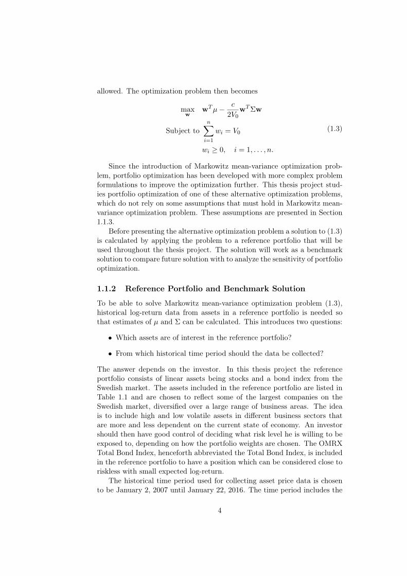
allowed. The optimization problem then becomes

maxw

wTµ− c

2V0wTΣw

Subject ton∑i=1

wi = V0

wi ≥ 0, i = 1, . . . , n.

(1.3)

Since the introduction of Markowitz mean-variance optimization prob-lem, portfolio optimization has been developed with more complex problemformulations to improve the optimization further. This thesis project stud-ies portfolio optimization of one of these alternative optimization problems,which do not rely on some assumptions that must hold in Markowitz mean-variance optimization problem. These assumptions are presented in Section1.1.3.

Before presenting the alternative optimization problem a solution to (1.3)is calculated by applying the problem to a reference portfolio that will beused throughout the thesis project. The solution will work as a benchmarksolution to compare future solution with to analyze the sensitivity of portfoliooptimization.

1.1.2 Reference Portfolio and Benchmark Solution

To be able to solve Markowitz mean-variance optimization problem (1.3),historical log-return data from assets in a reference portfolio is needed sothat estimates of µ and Σ can be calculated. This introduces two questions:

• Which assets are of interest in the reference portfolio?

• From which historical time period should the data be collected?

The answer depends on the investor. In this thesis project the referenceportfolio consists of linear assets being stocks and a bond index from theSwedish market. The assets included in the reference portfolio are listed inTable 1.1 and are chosen to reflect some of the largest companies on theSwedish market, diversified over a large range of business areas. The ideais to include high and low volatile assets in different business sectors thatare more and less dependent on the current state of economy. An investorshould then have good control of deciding what risk level he is willing to beexposed to, depending on how the portfolio weights are chosen. The OMRXTotal Bond Index, henceforth abbreviated the Total Bond Index, is includedin the reference portfolio to have a position which can be considered close toriskless with small expected log-return.

The historical time period used for collecting asset price data is chosento be January 2, 2007 until January 22, 2016. The time period includes the

4

global 2007 financial crisis, having its peak between approximately 2007 −2009 according to the time line in [8], where risky assets typically are morecorrelated, and some years afterwards where the market is starting to riseagain and the assets are less correlated.

Table 1.1: Swedish assets included in the reference portfolio and their corre-sponding business areas.

Asset name Business AreaAstraZeneca Health CareEricsson A TechnologyHennes & Mauritz B RetailICA Gruppen RetailNordea Bank BanksSAS Travel & LeisureSSAB A Basic ResourcesSwedish Match Personal & Household GoodsTeliaSonera TelecommunicationsVolvo Industrial Goods & ServicesTotal Bond Index Government bonds

The historical data is obtained from the Nasdaq OMX web page andconsists of daily prices for each of the assets in the reference portfolio1.Figure 1.1 depicts the historical price developments for the stocks to the leftand the Total Bond Index to the right.

2007 2008 2009 2010 2011 2012 2013 2014 2015 20160

100

200

300

400

500

600

700

AstraZ

Ericsson

H&M

ICA

Nordea

SAS

SSAB

Swedish Match

Telia

Volvo

2007 2008 2009 2010 2011 2012 2013 2014 2015 20164000

4500

5000

5500

6000

6500

OMRX Total Bond Index

Figure 1.1: Price developent for the stocks (left) and the bond index (right)in the reference portfolio during January 2, 2007-January 22, 2016.

From Figure 1.1 one can make several observations. For instance that17 data points for OMRX Total Bond Index was missing in the historical data set and

were linearly interpolated. The data is automatically adjusted for asset splits.

5

some companies managed the financial crisis better than others, for instanceNordea Bank, and that some assets have historically had a positive trend,such as Swedish Match, while other assets have had a negative trend, such asSAS. There are furthermore some assets that have changed very little in valueduring the time period of interest, for instance TeliaSonera, while other assetshave been more volatile, for instance ICA Gruppen. All these behaviors weredesired in the construction of the reference portfolio. Ultimately, the assetsincluded in a portfolio is up to the investor to decide and the referenceportfolio in this thesis project could have been selected differently. Thegeneral conclusions in the thesis project do however not directly depend onthe reference portfolio itself other than the fact that the weight vector andExpected Shortfall would change if other assets were used.

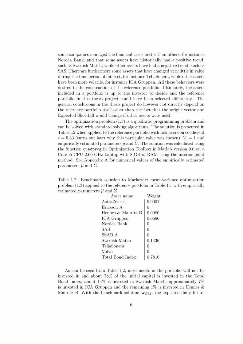
The optimization problem (1.3) is a quadratic programming problem andcan be solved with standard solving algorithms. The solution is presented inTable 1.2 when applied to the reference portfolio with risk aversion coefficientc = 5.33 (turns out later why this particular value was chosen), V0 = 1 andempirically estimated parameters µ and Σ. The solution was calculated usingthe function quadprog in Optimization Toolbox in Matlab version 9.0 on aCore i5 CPU 2.60 GHz Laptop with 8 GB of RAM using the interior pointmethod. See Appendix A for numerical values of the empirically estimatedparameters µ and Σ.

Table 1.2: Benchmark solution to Markowitz mean-variance optimizationproblem (1.3) applied to the reference portfolio in Table 1.1 with empiricallyestimated parameters µ and Σ.

Asset name WeightAstraZeneca 0.0001Ericsson A 0Hennes & Mauritz B 0.0080ICA Gruppen 0.0666Nordea Bank 0SAS 0SSAB A 0Swedish Match 0.1436TeliaSonera 0Volvo 0Total Bond Index 0.7816

As can be seen from Table 1.2, most assets in the portfolio will not beinvested in and about 78% of the initial capital is invested in the TotalBond Index, about 14% is invested in Swedish Match, approximately 7%is invested in ICA Gruppen and the remaining 1% is invested in Hennes &Mauritz B. With the benchmark solution wBM , the expected daily future

6

portfolio log-return is

E[wTBMR] = wT

BM µ = 2.0242 · 10−4 (1.4)

corresponding to a yearly2 expected portfolio log-return of 251 · wTBM µ ≈

5.08% and the daily portfolio variance is

σ2p = wT

BM ΣwTBM = 7.8354 · 10−6, (1.5)

meaning that the yearly portfolio variance is approximately 0.01%.

1.1.3 Stylized Assumptions in Markowitz Optimization Prob-lem

Markowitz mean-variance optimization problem (1.3) is theoretically impor-tant, but when applied to real financial portfolios it suffers from some stylizedassumptions that must hold for the problem formulation to be applicable.The first stylized assumption is that the log-returns have elliptical distribu-tion, which is not accurate enough when studying historical data, especiallyduring times of financial crisis where asset prices become more volatile andmore correlated. Furthermore, elliptical distributions are symmetric whichoften is not the case for historical log-returns where either the loss or thegain tail of the distribution is more prominent than the other tail. Therefore,parts of the empirical log-return distribution information is lost when mod-eling with elliptical distributions. The second stylized assumption is that theportfolio is linear, which is a major limitation. Often highly non-linear assetssuch as options or other financial derivatives are included in financial port-folios, that cannot be taken into consideration by Markowitz mean-varianceoptimization problem. With these drawbacks taken into account, alterna-tive portfolio optimization problems have recently become popular to study.This thesis project focus on the first drawback discussed but the problemcan easily be extended to include non-linear assets in the reference portfolioas well.

2There are about 251 trading days in a year on the Swedish market.

7

8

Chapter 2

Portfolio Optimization withExpected Shortfall

With the introduction to portfolio optimization in Chapter 1 I have so farconcluded that Markowitz mean-variance optimization problem (1.3) is notsufficient to employ in portfolio optimization unless the log-returns are el-liptically distributed, but due to its historical importance it may be usedas a benchmark problem. In this chapter, I introduce the concept of riskmeasures and construct an alternative optimization problem based on a riskmeasure better fit for modern portfolio optimization. The aim is to constructan appropriate portfolio optimization problem that does not rely on the styl-ized assumptions that must hold for Markowitz mean-variance optimizationproblem to be considered good.

2.1 Risk Measures

Financial risk can be measured in several different ways, but it is often de-sirable to measure risk in monetary units, meaning that the risk is expressedas buffer capital that needs to be added to a portfolio to protect it from un-desired outcomes. In Markowitz mean-variance optimization problem, therisk is measured as the variance of the future portfolio return. However,variance is not considered to be a very good risk measure in finance sinceit is defined as the expected squared deviation from the mean value andthus does not make difference between positive deviations, portfolio gain,and negative deviations, portfolio loss. Furthermore, standard deviation canonly be considered accurate enough to be translated into monetary risk if thefuture value of the portfolio value is approximately normal distributed. Thisis often a too strict assumption that simplifies the real portfolio log-returndistribution too much. Instead, it is often desirable to utilize a risk measurethat make difference between good and bad deviations from the expected fu-ture portfolio value. In this section I first present basic risk measure theory

9

and later specify two risk measures widely used in financial risk management.Generally, let ρ(X) be a function measuring the risk of a stochastic vari-

able X. Different risk measures have different properties and below is a listof such mathematical properties that are considered to be useful or desirable,together with brief explanations on how they can be interpreted.

1. Translation invariance. ρ(cR0 + X) = −c + ρ(X) for c ∈ R. Thismeans that adding the amount c with risk-free interest rate R0 to aportfolio reduces the risk equally much.

2. Monotonicity. If X2 < X1, then ρ(X1) ≤ ρ(X2). This means that ifwe know for certain that a portfolio X1 is greater than a portfolio X2

at a future time, then the first portfolio is considered to be less risky.

3. Convexity. ρ(λX1 +(1−λ)X2) ≤ λρ(X1)+(1−λ)ρ(X2), for any realλ ∈ [0, 1]. The risk measure rewards diversification, which means thatit takes into account that it often is wise to spread out the investmentin several risky positions, rather than investing everything in one.

4. Normalization. ρ(0) = 0. This means that it is acceptable to notinvest in risky assets at all, so that an empty portfolio is riskless.

5. Positive homogeneity. ρ(λX) = λρ(X) for λ ≥ 0. This means thatfor instance investing twice as much in one position is twice as risky.

6. Subadditivity. ρ(X1 + X2) ≤ ρ(X1) + ρ(X2). This property shouldalso be interpreted as that the risk measure rewards diversification. Acompany consisting of two business units is interpreted as less riskycompared to the two units considered as separate companies.

The reader is refered to the book [5, Ch. 6] by Hult, Lindskog, Hammarlidand Rehn for a more thorough presentation on general risk measure theoryand more comments on the above properties, as well as more on why varianceis considered a bad risk measure in finance.

A risk measure with the properties translation invariance and monotonic-ity is said to be a monetary measure of risk, and a risk measure considered toreplace variance in Markowitz mean-variance optimization problem shouldsatisfy at least these two properties. A risk measure that in addition totranslation invariance and monotonicity also satisfies convexity is said to bea convex risk measure. The convex risk measure family is thus a subset ofthe monetary risk measure family. Finally, a third risk measure family is thecoherent risk measure, where ρ(X) satisfies the properties translation invari-ance, monotonicity, positive homogeneity and subadditivity. It is easy to seethat a risk measure satisfying positive homogeneity also satisfies normaliza-tion by setting λ = 0. It can further be shown that positive homogeneityand convexity together implies subadditivity but not the reverse. Hence, a

10

coherent risk measure is also a convex risk measure but the opposite does notgenerally hold, so the coherent risk measure family is a subset of the convexrisk measure family and thus also a subset of the monetary risk measure fam-ily. When choosing an appropriate risk measure for a portfolio optimizationproblem replacing Markowitz mean-variance optimization problem one maytherefore consider both convex and coherent risk measures to be at least asgood as monetary risk measures. Below, two risk measures that are com-monly used in risk management are presented that are considered good infinancial mathematics.

2.1.1 Value-at-Risk

The first risk measure presented is the Value-at-Risk, abbreviated VaR.Value-at-Risk satisfies translation invariance, monotonicity and positive ho-mogeneity and is hence a monetary risk measure. The Value-at-Risk at levelp ∈ (0, 1) of a stochastic variable X is defined as

V aRp(X) = min{m ∈ R : P (mR0 +X < 0) ≤ p}.

If X is assumed to have right continuous and increasing cumulative distri-bution function F (x), which will be the case in this thesis project, it followsthat

V aRp(X) = min{m ∈ R : P (−X > mRo) ≤ p}= min{m ∈ R : P (L ≤ m) ≥ 1− p} = F−1

L (1− p)

where L = −X/R0 should be interpreted as the discounted loss. Hence, theValue-at-Risk of the stochastic variable X is the (1− p)-level quantile of theassociated discounted loss L.

A direct advantage with Value-at-Risk over traditional variance is that itcan be used when variance is not a relevant risk measure, for instance whenthe expected value of a distribution does not represent a fair picture of thedistributional appearance. Furthermore, since Value-at-Risk computes the(1−p)-level quantile of the discounted loss it accounts only for large losses butnot large gains and hence Value-at-Risk makes difference between negativeand positive deviations from the expected future portfolio value. However,since Value-at-Risk only look at a particular level (1−p) of the loss quantile,traders can take advantage of this to "hide" risky investments by makingthe losses more extreme so that the potential loss ends up further out in theloss distribution tail so that it is not discovered by Value-at-Risk. With thisstrategy, very risky portfolios could seem acceptable that otherwise wouldnot have been if the risk was visible for risk managers. This might result inthat companies are exposed to extremely large loss scenarios, although withrelatively small probability, but with the possible outcome that the companysuffers a huge loss and possibly bankruptcy.

11

2.1.2 Expected Shortfall

A better risk measure than Value-at-Risk in the sense that it takes intoaccount all losses located in the whole (1 − p)-level quantile tail of the lossdistribution is Expected Shortfall. For a stochastic variable X, the ExpectedShortfall, abbreviated ES, at level p ∈ (0, 1) is defined as

ESp(X) =1

p

∫ p

0V aRu(X)du =

1

1− q

∫ 1

qV aRu(L)du, (2.1)

where q = 1 − p. Expected Shortfall appears under several different namesin literature and with minor changes it is goes under the names Condi-tional Value-at-Risk (CVaR), Average Value-at-Risk (AVaR), Tail Value-at-Risk (TVaR), Expected Tail Loss (ETL) and Tail Conditional Expectation(TCE). Similarly to Value-at-Risk, if X has right continuous and increasingdistribution function F (x) then the Expected Shortfall has representation

ESp(X) =1

p

∫ p

0F−1L (1− u)du.

Since Expected Shortfall is defined through Value-at-Risk, it inherits theproperties of Value-at-Risk, being translation invariance, monotonicity andpositive homogeneity. It can further be shown that Expected Shortfall alsosatisfies subadditivity and is hence a coherent risk measure.

2.1.3 Contribution Expected Shortfall

In addition to the total portfolio risk, the investor might be interested inhow much each asset in the reference portfolio contributes to the total riskwhen allocating the capital. The contributions go under the names MarginalRisk, Contribution Risk and Euler Allocations/Decomposition and originatefrom Euler’s decomposition theorem. The theorem states that a function fof n variables x1, . . . , xn with continuous partial derivatives is homogenousof degree k if and only if the equation

n∑i=1

xi∂f

∂xi= kf

holds for all x1, . . . , xn ∈ D being an open domain. There exists severaldifferent approaches for decomposing the total portfolio risk but a naturaldecomposition given a homogenous risk measure would based on Euler’sdecomposition theorem be

ρ(X) =

n∑i=1

wi∂ρ(X)

∂wi. (2.2)

12

This is natural since exactly the total risk is decomposed, meaning thatthe sum of all contributions is exactly the total risk. Expected Shortfall is(positive) homogenous of degree 1 and a decomposition of the total portfolioExpected Shortfall is

ESp(X) =

n∑i=1

Ui∂ESp(X)

∂Ui

where U = (U1, . . . , Un)T is a vector of sensitivities defined by

Ui =n∑j=1

wj∂Fj(S(t))

∂Si(t),

wj being the asset weight and Fj(S(t)) is a financial instrument. The deriva-tive ∂ESp(X)/∂Ui should then be interpreted as the Euler Allocation forasset i.

Skoglund and Chen show in [18] that if the log-returns are assumed tohave multivariate normal distribution, the Euler Allocations can be calcu-lated analytically as

∂ESp(X)

∂U= λ(Φ−1(q))

∂σp∂U

. (2.3)

Here λ(x) is the hazard function for the normal distribution, defined as

λ(x) =φ(x)

1− Φ(x). (2.4)

and∂σp∂U

= (UTΣU)−1/2ΣU.

If the log-returns are modeled by their empirical distribution, the deriva-tive ∂ESp(X)/∂U does not exist since the portfolio distribution is discrete.In this case, we may use the results of Tasche [21] and approximate thederivative as

DESp(X)(wi) =

∑Dd=1 E[Li,.|Ld > Ls]∑D

d=1 1(Ld>Ls)

(2.5)

where {Li,d}n,Di=1,d=1 are the loss components, n being the number of assetsand D the amount of available loss scenarios, Li,. = (Li,1, . . . , Li,D)′, Ls isthe loss sample point corresponding to the p-level Value-at-Risk and

1(Ld>Ls) =

{1, Ld > Ls

0, otherwise.

In this thesis project the investment horizon is one day and the risk-freeinterest rate can be approximated to zero, which implies that Li = −Ri,

13

i.e. the log-returns with switched sign. With linear assets, the portfolio lossscenarios are then obtained by multiplying the weight vector with the lossvector, L = wTL = −wTR. Furthermore, by ordering the portfolio lossessuch that L1 > L2 > · · · > LD then the portfolio Value-at-Risk at level p,defined as the p-level loss quantile, is

V aRp(X) = Ls = L[Dp]+1 (2.6)

where [Dp] is the integer part of Dp.

2.1.4 Properties of the quantile function

Since the quantile function turns out to play a central role in both Value-at-Risk and Expected Shortfall, I here state two properties of the quantilefunction that will be used later.

Proposition 2.1 If g : R→ R is a nondecreasing function and left contin-uous, then for any random variable Z it holds that F−1

g(Z)(p) = g(F−1Z (p)) for

all p ∈ (0, 1).

Proposition 2.2 For any random variable X with continuous and strictlyincreasing density function FX , F−1

−X(p) = −F−1X (1− p) for all p ∈ (0, 1).

I refer the reader to Hult et al.[5, pp. 170-172] for complete proofs.

2.2 Portfolio Optimization Problem Formulation

In optimization, we are generally interested in finding the global extremepoint to a function under some constraining requirements. Convex optimiza-tion problems is a particularly nice family of optimization problems wherethere exists a unique optimal solution being the global extreme point. SinceExpected Shortfall is a coherent risk measure, it is also convex and hencean appealing risk measure to employ in financial optimization problems, op-posite to Value-at-Risk which does not satisfy the convexity property andmay therefore produce several local extreme points. With this in mind, itbecomes natural to use Expected Shortfall rather than Value-at-Risk as riskmeasure in a portfolio optimization problem. Additionally, since ExpectedShortfall does not demand elliptically distributed log-returns or linear port-folios, it does not rely on the stylized assumptions that must be assumed inMarkowitz mean-variance optimization problem. In this section I formulatethe portfolio optimization problem based on minimizing Expected Shortfallthat will be the subject of study in the remaining part of this thesis project.

Simply minimizing the Expected Shortfall in a portfolio optimizationproblem is trivial without constraining equations and in a market consistingof only risky assets the solution would be to not invest at all. Therefore,

14

a reasonable initial constraint would be that the entire initial capital V0

must be invested in the market. Additionally, it is common to constrain theasset allocations to long positions, i.e. wi ≥ 0, i = 1, . . . , n. The portfoliooptimization problem can then be stated mathematically as

minw

ESp(wTR)

Subject ton∑i=1

wi = V0

wi ≥ 0, i = 1, . . . , n,

where n is the number of assets available in the portfolio.Often, investors are not interested in only minimizing the risk, but they

want some reward for exposing their capital to risk. Therefore, investors addthe constraint that the future expected portfolio (log)-return should be largersome threshold (log-)return θ. The optimization problem then becomes

minw

ESp(wTR)

Subject to wTµ ≥ θn∑i=1

wi = V0

wi ≥ 0, i = 1, . . . , n.

(2.7)

The above problem formulation will be the foundation of this thesis project.Next I remark on a special case when (2.7) have the same solution as thebenchmark solution to Markowitz mean-variance optimization problem andthen I state a few general model assumptions that is used when later solving(2.7) numerically. In Section 2.3 I show that the portfolio optimizationproblem can be approximated and solved by ordinary linear programming.

In section 2.1.3 it was said that a natural decomposition of the totalportfolio risk is obtained by calculating the Euler Allocations since thenthe risk contributions sum up to exactly the total risk. But this propertycan be achieved for any risk decomposition method by simply normalizing.However, Tasche proves in [20] that Euler decomposition is the only riskdecomposition method that is consistent with (local) portfolio optimizationwhich motivates the benefits of using Euler decomposition in this thesisproject.

In portfolio optimization the Euler Allocations have a second field ofapplication in addition to measuring the risk contribution from a specificasset to the total portfolio risk. The famous Sharpe ratio, introduced bySharpe [17], relates the expected portfolio (log)-return to the risk as

S =wTµ

ρ(2.8)

15

and the larger Sharpe ratio the better is the investment. Similarly to thedecomposition of the portfolio risk a natural decomposition of the Sharperatio is to define

S∗i =wiµi

wi∂ρ∂wi

(2.9)

as the marginal Sharpe ratio of asset i, i = 1, . . . , n. An asset should thenbe considered a good investment if the marginal Sharpe ratio is large. Withthe marginal Sharpe ratio as argument for investing in an asset or not, it canbe seen that the only information an investor requires for (local) portfoliooptimization is the expected log-return and Euler Allocation. This observa-tion will be used later when attempting to analyze the optimal solutions tothe portfolio optimization problem with Expected Shortfall.

2.2.1 Remark: Elliptically distributed log-returns

The following remark points out a special case where portfolio optimizationproblem (2.7) can be simplified to a modified version of Markowitz mean-variance problem (1.3). This is important since the solution to (2.7) shouldin this case be the same as the benchmark solution in Table 1.2.

Consider a scenario where the vector of log-returns R is assumed to beelliptically distributed with mean µ and covariance matrix Σ. Then R canbe represented as

Rd= µ+WAZ

where A is a matrix such that AAT = Σ and Z ∈ N(0, Id), Id being thed-dimensional identity matrix, is independent of W ≥ 0. The portfolio log-return is then

wTR = wTµ+√wTΣwWZ1 (2.10)

where I have used a standard property for spherically distributed randomvariables and Z1 is univariate standard normal distributed. Minimizing theExpected Shortfall then yields

minw

ESp(wTR) = min

w−1

p

∫ p

0F−1wTR

(u)du

= minw−wTµ−

√wTΣw

1

p

∫ p

0F−1WZ1

(u)du

where I have used both Proposition 2.1 and Proposition 2.2. Now, sinceminimizing −f(w) corresponds to maximizing f(w), portfolio optimization

16

problem (2.7) with elliptically distributed log-returns can be written

maxw

wTµ− c

2V0

√wTΣw

Subject to wTµ ≥ θn∑i=1

wi = V0

wi ≥ 0, i = 1, . . . , n,

where

c = −2V0

p

∫ p

0F−1WZ1

(u)du. (2.11)

Note the similarity between the above special case and Markowitz mean-variance optimization problem (1.3). Optimization problem (2.7) can in thespecial case considered hence be rewritten as an optimization problem withsolution equivalent to that of the standard quadratic optimization problem.

2.2.2 General Problem Assumptions

This section presents some assumptions that need to be specified for theportfolio optimization problem (2.7) to be numerically solvable. The as-sumptions stated are used when solving the portfolio optimization problemunless otherwise explicitly stated.

Assumption 1 The investor’s initial capital V0 = 1. This was already assumed whencalculating the benchmark solution and is used to simplify the analysiswork of the solutions since the asset weights wi can be seen as propor-tions of the whole initial capital rather than monetary weights. Thesolution is then easily interpreted for arbitrary initial capital V0.

Assumption 2 The portfolio lives for one day. This means that the goal is to investoptimally for one day ahead, which is convenient since the historicaldata consists of daily log-returns calculated using (1.1).

Assumption 3 p = 0.01 (q = 0.99). Banks often use the p-value p = 0.005 but othercommon levels are p = 0.01 and p = 0.05. The smaller value p, themore unlikely it is to be exposed to a loss larger than the calculatedExpected Shortfall. p = 0.01 means that with a portfolio life of oneday, one would expect the loss to be larger than the Expected Shortfallin 1 out of every 100 days. Plugging in p = 0.01 in (2.11) yields withZ1 being standard normal distributed and W = 1

c = − 2

0.01

∫ 0.01

0Φ−1(u)du =

2φ(Φ−1(0.01))

0.01= 5.33, (2.12)

17

where φ(x) denotes the probability density function of the standardnormal distribution. This explains why the risk aversion coefficientc = 5.33 was used earlier in the benchmark solution.

Assumption 4 The threshold for acceptable expected daily portfolio log-return is θ =2.0242·10−4 corresponding to 5.08% yearly log-return. This is the sameexpected portfolio log-return as for the benchmark solution calculatedin (1.4). The value of θ is ultimately up to the investor to decide, beinga trade-off between return and risk, where larger θ could expose theinvestor to larger risk. The impact on the optimal solution of varyingθ is analyzed in Section 4.1.

When analyzing the Expected Shortfall of a portfolio it is common tolook at the relative Expected Shortfall defined as the ratio

ESrel =ES

Portfolio market value.

With Assumption 1 the portfolio market value is 1 implying that in thisthesis project the relative Expected Shortfall equals the Expected Short-fall calculated when solving the portfolio optimization problem (2.7) whichsimplifies the analysis.

2.3 Rockafellar and Uryasev simplification

Since the definition of Expected Shortfall involves an integral of the Value-at-Risk, being the quantile function of the loss distribution, it is difficultto work directly with and optimize (2.1). Rockafellar and Uryasev providein [15] two theorems that simplify problem formulation (2.7) much. Thissection presents this simplification.

The key is to characterize ESp(X) and VaRp(X) with the auxiliary func-tion Hp(w, α) on W,Rm defined by

Hp(w, α) = α+1

1− q

∫R∈Rm

[L(w,R)− α]+f(R)dR (2.13)

where

[x]+ =

{x, x > 0

0, x ≤ 0

and f(R) is the probability density function of the log-return vector R. Thetheorems regarding the characterization are central in this thesis project andare stated below.

18

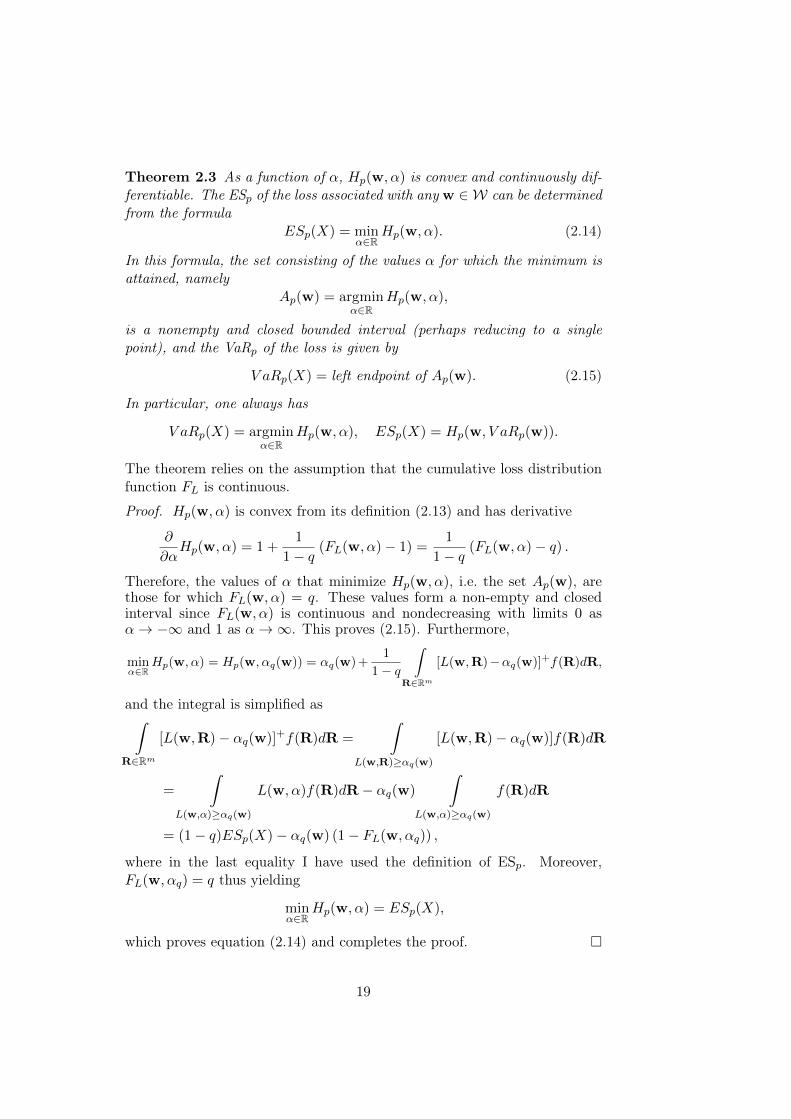
Theorem 2.3 As a function of α, Hp(w, α) is convex and continuously dif-ferentiable. The ESp of the loss associated with any w ∈ W can be determinedfrom the formula

ESp(X) = minα∈R

Hp(w, α). (2.14)

In this formula, the set consisting of the values α for which the minimum isattained, namely

Ap(w) = argminα∈R

Hp(w, α),

is a nonempty and closed bounded interval (perhaps reducing to a singlepoint), and the VaRp of the loss is given by

V aRp(X) = left endpoint of Ap(w). (2.15)

In particular, one always has

V aRp(X) = argminα∈R

Hp(w, α), ESp(X) = Hp(w, V aRp(w)).

The theorem relies on the assumption that the cumulative loss distributionfunction FL is continuous.

Proof. Hp(w, α) is convex from its definition (2.13) and has derivative

∂

∂αHp(w, α) = 1 +

1

1− q(FL(w, α)− 1) =

1

1− q(FL(w, α)− q) .

Therefore, the values of α that minimize Hp(w, α), i.e. the set Ap(w), arethose for which FL(w, α) = q. These values form a non-empty and closedinterval since FL(w, α) is continuous and nondecreasing with limits 0 asα→ −∞ and 1 as α→∞. This proves (2.15). Furthermore,

minα∈R

Hp(w, α) = Hp(w, αq(w)) = αq(w) +1

1− q

∫R∈Rm

[L(w,R)−αq(w)]+f(R)dR,

and the integral is simplified as∫R∈Rm

[L(w,R)− αq(w)]+f(R)dR =

∫L(w,R)≥αq(w)

[L(w,R)− αq(w)]f(R)dR

=

∫L(w,α)≥αq(w)

L(w, α)f(R)dR− αq(w)

∫L(w,α)≥αq(w)

f(R)dR

= (1− q)ESp(X)− αq(w) (1− FL(w, αq)) ,

where in the last equality I have used the definition of ESp. Moreover,FL(w, αq) = q thus yielding

minα∈R

Hp(w, α) = ESp(X),

which proves equation (2.14) and completes the proof. �

19

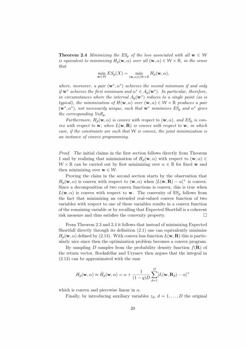
Theorem 2.4 Minimizing the ESp of the loss associated with all w ∈ Wis equivalent to minimizing Hp(w, α) over all (w, α) ∈ W × R, in the sensethat

minw∈W

ESp(X) = min(w,α)∈W×R

Hp(w, α),

where, moreover, a pair (w∗, α∗) achieves the second minimum if and onlyif w∗ achieves the first minimum and α∗ ∈ Ap(w∗). In particular, therefore,in circumstances where the interval Ap(w∗) reduces to a single point (as istypical), the minimization of H(w, α) over (w, α) ∈ W × R produces a pair(w∗, α∗), not necessarily unique, such that w∗ minimizes ESp and α∗ givesthe corresponding VaRp.

Furthermore, Hp(w, α) is convex with respect to (w, α), and ESp is con-vex with respect to w, when L(w,R) is convex with respect to w, in whichcase, if the constraints are such that W is convex, the joint minimization isan instance of convex programming.

Proof. The initial claims in the first section follows directly from Theorem1 and by realizing that minimization of Hp(w, α) with respect to (w, α) ∈W × R can be carried out by first minimizing over α ∈ R for fixed w andthen minimizing over w ∈ W.

Proving the claim in the second section starts by the observation thatHp(w, α) is convex with respect to (w, α) when [L(w,R) − α]+ is convex.Since a decomposition of two convex functions is convex, this is true whenL(w, α) is convex with respect to w. The convexity of ESp follows fromthe fact that minimizing an extended real-valued convex function of twovariables with respect to one of these variables results in a convex functionof the remaining variable or by recalling that Expected Shortfall is a coherentrisk measure and thus satisfies the convexity property. �

From Theorem 2.3 and 2.4 it follows that instead of minimizing ExpectedShortfall directly through its definition (2.1) one can equivalently minimizeHp(w, α) defined by (2.13). With convex loss function L(w,R) this is partic-ularly nice since then the optimization problem becomes a convex program.

By sampling D samples from the probability density function f(R) ofthe return vector, Rockafellar and Uryasev then argues that the integral in(2.13) can be approximated with the sum

Hp(w, α) ≈ Hp(w, α) = α+1

(1− q)D

D∑d=1

[L(w,Rd)− α]+

which is convex and piecewise linear in α.Finally, by introducing auxiliary variables zd, d = 1, . . . , D the original

20

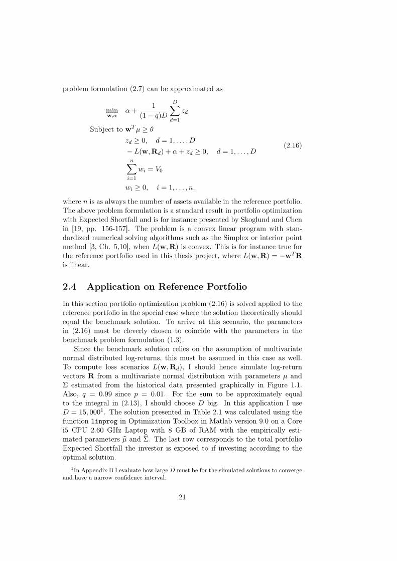
problem formulation (2.7) can be approximated as

minw,α

α+1

(1− q)D

D∑d=1

zd

Subject to wTµ ≥ θzd ≥ 0, d = 1, . . . , D

− L(w,Rd) + α+ zd ≥ 0, d = 1, . . . , Dn∑i=1

wi = V0

wi ≥ 0, i = 1, . . . , n.

(2.16)

where n is as always the number of assets available in the reference portfolio.The above problem formulation is a standard result in portfolio optimizationwith Expected Shortfall and is for instance presented by Skoglund and Chenin [19, pp. 156-157]. The problem is a convex linear program with stan-dardized numerical solving algorithms such as the Simplex or interior pointmethod [3, Ch. 5,10], when L(w,R) is convex. This is for instance true forthe reference portfolio used in this thesis project, where L(w,R) = −wTRis linear.

2.4 Application on Reference Portfolio

In this section portfolio optimization problem (2.16) is solved applied to thereference portfolio in the special case where the solution theoretically shouldequal the benchmark solution. To arrive at this scenario, the parametersin (2.16) must be cleverly chosen to coincide with the parameters in thebenchmark problem formulation (1.3).

Since the benchmark solution relies on the assumption of multivariatenormal distributed log-returns, this must be assumed in this case as well.To compute loss scenarios L(w,Rd), I should hence simulate log-returnvectors R from a multivariate normal distribution with parameters µ andΣ estimated from the historical data presented graphically in Figure 1.1.Also, q = 0.99 since p = 0.01. For the sum to be approximately equalto the integral in (2.13), I should choose D big. In this application I useD = 15, 0001. The solution presented in Table 2.1 was calculated using thefunction linprog in Optimization Toolbox in Matlab version 9.0 on a Corei5 CPU 2.60 GHz Laptop with 8 GB of RAM with the empirically esti-mated parameters µ and Σ. The last row corresponds to the total portfolioExpected Shortfall the investor is exposed to if investing according to theoptimal solution.

1In Appendix B I evaluate how large D must be for the simulated solutions to convergeand have a narrow confidence interval.

21

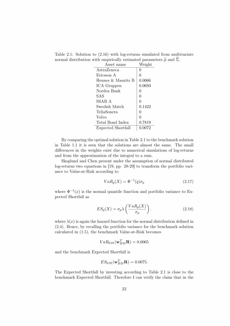
Table 2.1: Solution to (2.16) with log-returns simulated from multivariatenormal distribution with empirically estimated parameters µ and Σ.

Asset name WeightAstraZeneca 0Ericsson A 0Hennes & Mauritz B 0.0066ICA Gruppen 0.0693Nordea Bank 0SAS 0SSAB A 0Swedish Match 0.1422TeliaSonera 0Volvo 0Total Bond Index 0.7819

Expected Shortfall 0.0072

By comparing the optimal solution in Table 2.1 to the benchmark solutionin Table 1.1 it is seen that the solutions are almost the same. The smalldifferences in the weights exist due to numerical simulations of log-returnsand from the approximation of the integral to a sum.

Skoglund and Chen present under the assumption of normal distributedlog-returns two equations in [19, pp. 28-29] to transform the portfolio vari-ance to Value-at-Risk according to

V aRp(X) = Φ−1(q)σp (2.17)

where Φ−1(x) is the normal quantile function and portfolio variance to Ex-pected Shortfall as

ESp(X) = σpλ

(V aRp(X)

σp

). (2.18)

where λ(x) is again the hazard function for the normal distribution defined in(2.4). Hence, by recalling the portfolio variance for the benchmark solutioncalculated in (1.5), the benchmark Value-at-Risk becomes

V aR0.01(wTBMR) = 0.0065

and the benchmark Expected Shortfall is

ES0.01(wTBMR) = 0.0075.

The Expected Shortfall by investing according to Table 2.1 is close to thebenchmark Expected Shortfall. Therefore I can verify the claim that in the

22

special case of multivariate normal distributed log-returns, portfolio opti-mization problem (2.7) is indeed identical to Markowitz mean-variance opti-mization problem (1.3). Furthermore, since the two optimization problemsare connected only by the risk aversion coefficient c, calculated as (2.11)for all elliptical distributions, it is clear that Markowitz mean-variance opti-mization problem is a special case of portfolio optimization with ExpectedShortfall for all elliptical distributions. Since portfolio optimization with Ex-pected Shortfall does not rely on the stylized assumptions that Markowitzmean-variance optimization problem requires, (2.7) is a more general prob-lem formulation that can be applied to more general investment situationswith possibility to include non-linear assets or model the log-returns withasymmetric distributions for instance. In this thesis project I focus on themodeling of asset log-returns with non-elliptical distributions.

23

24

Chapter 3

Portfolio Optimization UnderUncertainty

Recall that the future portfolio log-return is a linear function of portfolioweights wi and random log-returns Ri, i = 1, . . . , n. Since the set of histor-ical log-returns is finite, there will be uncertainty in estimated parameterssuch as the expected log-return vector and covariance matrix. Parameteruncertainty might in turn cause large errors in the final portfolio decisiondeviating much from the true optimal asset allocations. Parameter uncer-tainty can be thought of as a sub class to the larger family of model uncer-tainty, with may also include uncertainty in distribution model. Distributionuncertainty originates from the fact that the true distribution of empiricallog-returns is unknown and must be approximated. The approximation canoften not be made perfect and there exists uncertainty in the distributionapproximation.

As mentioned in Section 2.2.1, when log-returns are assumed to have el-liptical distribution, portfolio optimization problem (2.7) has solution thatis equal to that of Markowitz mean-variance optimization problem. In thisspecial case, there is no need to simulate log-return outcomes since the solu-tion only depends on the expected log-return vector and covariance matrix.When the log-returns are assumed to be other than elliptically distributedsproblem (2.7) does not have analytical solution and simulations of log-returnsis necessary. The simulations introduce another source of uncertainty calledstatistical uncertainty. By the nature of simulations, one cannot be certainthat the outcomes reflect a fair picture of the distribution they were drawnfrom, which is why statistical uncertainty is a problem. The remaining partof this thesis project will study portfolio optimization with Expected Short-fall under both model and statistical uncertainty and present approaches onhow to handle optimization under those uncertainties.

25

3.1 Model Uncertainty

Markowitz mean-variance optimization problem assumes the expected log-return vector µ and covariance matrix Σ to be known and the same holdsfor the portfolio optimization problem (2.7). However in real applicationsthe parameters are often estimated from historical market data, as in thisthesis project. Since there is only a limited amount of historical data avail-able on the market, the expected log-return vector has to be estimated bythe empirical mean vector and similarly the covariance matrix must also beapproximated. One cannot be certain that the approximated parametersequals the true market parameters and hence there exists model uncertaintyin the parameters when solving the portfolio optimization problem yieldinguncertainty in the optimal solution.

A long established problem in portfolio optimization is referred to as theproblem of error maximization, discussed by Scherer in [16, pp. 185-186].The problem origins from that the optimization algorithm tends to selectassets with the best properties, in this case high log-return and low varianceand correlation, and not select assets with the worst properties. These arethe assets where estimation errors in µ and Σ are likely to be largest, withstrong dependence on outliers in the data. Hence the optimal solution willhave strong dependence on parameter uncertainty, where positive estimationerror leads to over-weighted assets and negative estimation error leads tounder-weighted assets.

In addition to parameter uncertainty, the multivariate distribution of theempirical log-returns can generally only be approximated, leading to uncer-tainty in distribution in the model. Different distributions are more or lesssuccessful in modeling historical data and where some are better at model-ing the tails of the empirical distribution, others are better at capturing thebehavior in the center of the empirical distribution. A perfect distributionfit on the entire empirical distribution is generally not possible to find andhence uncertainty in distribution must be regarded as a relevant factor inthe model.

In the 1990s, two approaches were developed to tackle model uncertainty.One approach is called robust statistics, which involves removing or down-weighting what is thought of as being outliers in the empirical data set. Thesecond approach is the concept of robust optimization, which will be consid-ered in this thesis project. Robust optimization can intuitively be thought ofas attempting to optimize the worst-case scenario given a confidence region.Traditionally, parameter uncertainty in Markowitz mean-variance optimiza-tion problem has received a lot of attention from the robust optimizationcommunity but less has been said about distribution uncertainty. This the-sis project contributes to the robust optimization community by studyingworst-case scenario based robust optimization of portfolio optimization prob-lem (2.16) under different distribution models. First I will perform a case

26

study on robust optimization under elliptical distributions and then moveon to study robust optimization under asymmetric log-return distributions.

A third possibility for model uncertainty is that the model itself is wrong.For instance, there might exist liquidity risk in assets, invalidating the trans-lation invariance property of the risk measure, included in the portfolio whichis not covered by the model, or it could be that the covariance matrix is de-pendent on time and state of economy. These types of model uncertaintiescan be harder to evaluate directly without changing the entire problem for-mulation and will not be considered in this thesis project.

3.1.1 Introduction to Robust Optimization

This section introduces robust optimization and specifies what is meant byworst-case scenario based robust optimization. Generally, let f(w;X,a) andgk(w;X,b), k = 1, . . . ,m be functions of the weight vector w, where X isa stochastic variable with cumulative distribution function FX(x) and a,bare parameters and consider the optimization problem

minw

f(w;X,a)

Subject to gk(w;X,b) ≤ gk,0, k = 1, . . . ,m,

where gk,0 k = 1, . . . ,m are constants. If f(w;X,a) is a convex function andthe constraining equations span a convex region, there exists a unique globaloptimal solution that can be found using standard optimization algorithms.

Now suppose that there is some uncertainty in the parameters a,b and inthe cumulative distribution function FX(x) and it is only known that a ∈ A,b ∈ B and FX(x) ∈ F for some sets A,B and family of distributions F . Theproblem formulation then becomes

minw

f(w;X,a)

Subject to gk(w;X,b) ≤ gk,0, k = 1, . . . ,m

a ∈ A,b ∈ B, FX(x) ∈ F .

Since ordinary optimization problems require parameters to be known, thisproblem cannot be solved with traditional optimization methods. Instead,the concept of robust optimization has been developed. The general objec-tive of robust optimization is to compute solutions that ensure feasibilityindependent of the parameters and distribution included in the uncertaintysets. Note that there is a key difference between robust optimization and sen-sitivity analysis, which is typically applied after the optimization to studythe change in objective function under small variations in the underlyingdata. With robust optimization, the goal is instead to compute solutionswhen the uncertainty is included in the problem formulation, prior to opti-mization. Similarly to ordinary optimization, if f(w;X,a) and gk(w;X,b)

27

are convex functions and A,B,F are convex sets, the robust optimizationproblem is particularly nice since when an extreme point is found, we knowit is the global optimal solution.

There are different approaches on how to solve a robust optimizationproblem, and one of the most commonly used approaches in portfolio opti-mization is the worst-case scenario based robust optimization approach in-troduced by Tütüncü and König in [22]. They argue it is a good idea to solvethe robust optimization problem by first finding the worst-case scenarios forthe parameters given the uncertainty sets and then consider the resultingoptimization problem with these worst-case scenario parameters and solveit with ordinary optimization algorithms. For instance, if the worst-casescenario is attained for the smallest a in the uncertainty set A and for thelargest b in the uncertainty set B then the worst-case scenario based robustoptimization problem would be

minw,a∈A

f(w;X,a)

Subject to maxb∈B

gk(w;X,b) ≤ gk,0, k = 1, . . . ,m

under the additional constraint thatX is drawn from the worst-case distribu-tion, measured in some way, that is included in the distribution uncertaintyset F .

Since the worst-case scenario based robust optimization approach is widelyused in robust portfolio optimization problems, it is used in this thesis projectas well. Section 4.2 discuss in greater detail the effect of interpreting robustoptimization as finding the worst-case scenario and then optimize the result-ing worst-case scenario optimization problem.

3.1.2 Robust Optimization with Elliptical Distributions

Before presenting the worst-case scenario based robust version of (2.16) Imention some work that historically has been done on robust optimizationof Markowitz mean-variance optimization problem. Lobo and Boyd discussin [11] a robust variant of Markowitz mean-variance problem with uncertaincovariance matrix Σ. The problem is presented as

minw

maxΣ∈S

wTΣw

Subject to wTµ ≥ Rminn∑i=1

wi = 1

wi ≥ wmin

and aims at finding the portfolio weights that minimize the total portfoliovariance with the worst-case covariance matrix. The authors assume that

28

the investor is ambiguous about the covariance matrix and have several pos-sible candidates. The robust problem is discussed with box and ellipsoidalconstraints on the covariance matrix, mathematically as

Sbox ={

Σ ∈ Sn+|Σij,low ≤ Σij ≤ Σij,high, i, j = 1, . . . , n}

Sellipsoid ={

Σ ∈ Sn+|(s− s)TQ(s− s) ≤ 1},

where s is a vector representation of the upper triangular elements of Σ, s isthe corresponding empirically estimated vector and Q is the second momentof the Wishart distribution for the empirically estimated covariance matrix.A similar robust optimization problem is also presented where instead thebox and ellipsoidal uncertainty sets constrain the mean log-return vector µ,mathematically written as

Mbox = {µ ∈ Rn|µi,low ≤ µi ≤ µi,high, i = 1, . . . , n}Mellipsoid =

{µ ∈ Rn|(µ− µ)TS−1(µ− µ) ≤ 1

},

where S is a scaled version of Σ and µ is the empirically estimated expectedlog-return vector. Both the box and ellipsoidal uncertainty set are convexsets so they are attractive from an optimization perspective. Ye, Parpas andRustem [23] takes the problem formulation by Lobo and Boyd further andpropose a problem where both µ and Σ are uncertain so that the optimizationproblem becomes

minw

maxΣ∈S

wTΣw

Subject to minµ∈M

wTµ ≥ Rminn∑i=1

wi = 1

wi ≥ wmin

and the objective is to find the portfolio weights that minimize the risk givenworst-case scenarios in both expected log-return and covariance.

The worst-case scenario based robust version of problem (2.16) is noweasy to formulate in a similar manner. Let the covariance matrix Σ and themean log-return vector µ be estimates from historical data of the uncertainparameters Σ and µ and assume we know that the true parameters aresomewhere in the uncertainty sets M,S. The robust version of portfolio

29

optimization problem (2.16) with linear loss function is then given by

minw,α

α+1

(1− q)D

D∑d=1

zd

Subject to minµ∈M

wTµ ≥ θ

zd ≥ 0, d = 1, . . . , D

minµ∈M

maxΣ∈S

wTRd + α+ zd ≥ 0, d = 1, . . . , D

n∑i=1

wi = V0

wi ≥ 0, i = 1, . . . , n

(3.1)

and the log-return vectors Rd, d = 1, . . . , D are simulated from some dis-tribution that is interpreted as the worst one of all distributions included inthe distribution uncertainty set F .

To solve (3.1) numerically, the uncertainty setsM,S must be specified sothat the worst-case scenarios can be found, and the distribution uncertaintyset F must be defined. I begin by constructing the uncertainty setsM,S.

To ensure that the robust optimization problem remains convex, I letM,S be boxes or ellipsoids as discussed by Lobo and Boyd. One approachto construct a box uncertainty set for µ is to add or subtract some term±ε|µi|to each empirically estimated element µi. This yields the box uncertaintyset

Mbox = {µ ∈ Rn : µ = µ± ε|µ|}

and the worst-case scenario expected log-return vector would then be

µ(box)min = µ− ε|µ|. (3.2)

In this thesis project I have set ε = 0.20. A reasonable sanity check isto investigate if µ(box)

min lies within the approximate 95% confidence intervalcalculated from the historical data to make sure that it is not unrealisticallyfar from the empirically estimated parameter. With the data used in thisthesis project and ε = 0.20, µ(box)

min does indeed lie within the 95% confidenceinterval.

To calculate the worst-case scenario covariance matrix requires a bit morethought process. It is not possible to employ the same strategy as whencalculating a box uncertainty set for µ since this could result in a non-invertible matrix which is not desired. There are several methods to definethe worst-case covariance matrix and the general idea is that one wants toincrease the eigenvalues and rotate the eigenvectors by some angle so thatthe resulting matrix is scaled and oriented worse than the original covariancematrix. One approach that does this implicitly is to study the historical price

30

development for the assets in the reference portfolio and locate a time periodwhere the assets seem the most correlated. Typically this occurs during timesof financial crisis. Looking at the asset price development in Figure 1.1, itseems as the assets in the reference portfolio are the most correlated during2007 − 2009 where most asset prices have a negative trend, which fits wellwith the time line for the financial crisis presented in [8]. Therefore, theworst-case scenario covariance matrix originating from a box uncertainty setis defined with basis on the financial crisis and taken as the covariance matrixestimated from historical data from the first trading day of 2007 until thelast trading day of 2009, i.e.

Σ(box)max = Σ between January 2, 2007 – December 30, 2009. (3.3)

Since an empirically estimated covariance matrix is always positive semi-definite, this approach ensures an invertible worst-case scenario covariancematrix. Throughout the remaining part of the thesis project I refer to theworst-case scenario parameters µ(box)

min and Σ(box)max given by (3.2) and (3.3)

respectively as "box uncertainty parameters". See Appendix A for numericalvalues.

With ellipsoidal uncertainty sets the elements depend on each other whichmakes it harder to find the worst-case scenarios µmin and Σmax. The valueof one element restricts the range of values the other elements can take soit is not possible to find the worst-case scenario for each element separatelywithout taking into account the other element values. One approach tofind the worst-case scenario expected log-return vector originating from anellipsoidal uncertainty set is however to solve the optimization problem

µ(ellipsoidal)min =

minµ

µ− µ

Subject to (µ− µ)TS−1(µ− µ) ≤ 1.(3.4)

In this thesis project, the above optimization problem is solved with S−1 =100Σ−1 to limit the resulting worst-case scenario parameter µmin to notdeviate too much from µ. In a similar way, the worst-case scenario covariancematrix originating from an ellipsoidal uncertainty set can be obtained bysolving the optimization problem

Σ(ellipsoidal)max =

max

ss− s

Subject to (s− s)TQ(s− s) ≤ 1

s ≤ (n−1)sχ2

0.975

diag(Σ(ellipsoidal)max ) ≥ 0.

(3.5)

The two last constraints are posed to ensure that Σmax is not too far fromΣ and so that all variances are positive. In this thesis project the second

31

moment of the Wishart distribution, Q, is estimated by simulating 10, 000covariance matrices from the Wishart distribution and then calculate thecovariance matrix for all pairwise elements in the simulated covariance ma-trices. The solution to (3.5) might not be positive semi-definite which is arequirement for the portfolio optimization problem to be solvable. In thatcase Rebonato and Jäckel present in [14] a general methodology to find theclosest symmetric and positive semi-definite matrix given a non positive semi-definite matrix that can be used to obtain a feasible covariance matrix. Themethod involves spectral decomposition of the matrix and setting negativeeigenvalues to zero. Throughout the remaining part of the thesis project Irefer to the worst-case parameters µ(ellipsoidal)

min and Σ(ellipsoidal)max given by (3.4)

and (3.5) respectively as "ellipsoidal uncertainty parameters". See AppendixA for numerical values.

Regarding the distribution uncertainty set F , the thesis project first con-siders elliptical distributions with the historically popular normal distribu-tion and Student’s t distribution with different degrees of freedom, i.e.

Felliptical = {N(µ,Σ), t(µ,Σ, ν)} , (3.6)

and later on considers asymmetric log-return distributions with the general-ized Pareto distribution.

For the elliptical distributions in Felliptical, it is easy to determine theworst-case scenario distribution. Since the Student’s t distribution has heav-ier tails than the normal distribution, the normal distribution is ruled outdirectly as the worst-case scenario distribution, having lower probability ofencountering extremely large losses. For the Student’s t distribution, thevariance is undefined for ν < 2, infinite for ν = 2 and for increasing ν > 2 thevariance is decreasing. Hence, the smaller the degrees of freedom, the heav-ier the tails of the distribution and the greater is the variance and ExpectedShortfall. The worst-case scenario distribution that ensures that varianceexists is hence Student’s t distribution with lim

ν↘2ν ≈ 2.1 degrees of freedom.

Since not much work has been done by the robust optimization commu-nity on uncertainty in distribution, it would be interesting to analyze thebehavior of the solution to (3.1) under different distributions. Therefore,instead of simply solving (3.1) with the worst-case distribution in Felliptical,this thesis project contributes to the robust portfolio optimization commu-nity with a case study by solving the problem for each of the distributionsin Felliptical with both box and ellipsoidal uncertainty parameters. This isdone in the two following sub sections.

3.1.2.1 Solution with Normal Distributed Log-returns

This section presents solutions to the robust portfolio optimization prob-lem (3.1) applied to the reference portfolio with log-return vectors Rd, d =

32

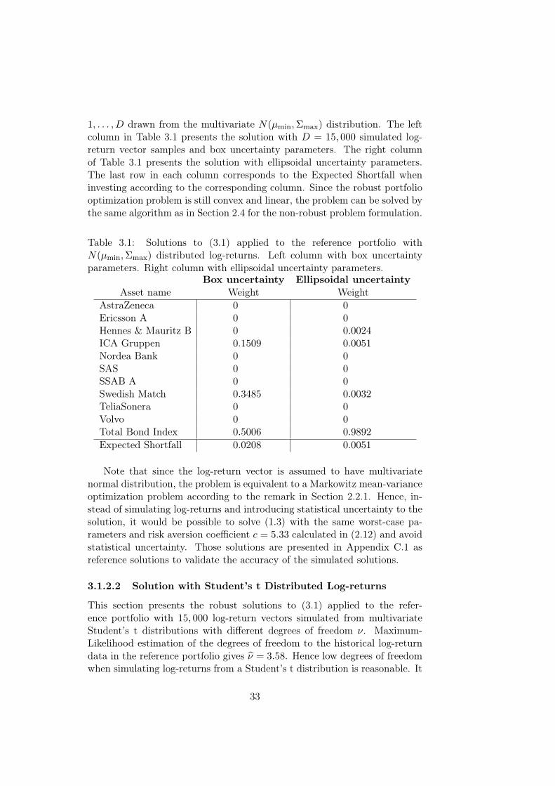
1, . . . , D drawn from the multivariate N(µmin,Σmax) distribution. The leftcolumn in Table 3.1 presents the solution with D = 15, 000 simulated log-return vector samples and box uncertainty parameters. The right columnof Table 3.1 presents the solution with ellipsoidal uncertainty parameters.The last row in each column corresponds to the Expected Shortfall wheninvesting according to the corresponding column. Since the robust portfoliooptimization problem is still convex and linear, the problem can be solved bythe same algorithm as in Section 2.4 for the non-robust problem formulation.

Table 3.1: Solutions to (3.1) applied to the reference portfolio withN(µmin,Σmax) distributed log-returns. Left column with box uncertaintyparameters. Right column with ellipsoidal uncertainty parameters.

Box uncertainty Ellipsoidal uncertaintyAsset name Weight Weight

AstraZeneca 0 0Ericsson A 0 0Hennes & Mauritz B 0 0.0024ICA Gruppen 0.1509 0.0051Nordea Bank 0 0SAS 0 0SSAB A 0 0Swedish Match 0.3485 0.0032TeliaSonera 0 0Volvo 0 0Total Bond Index 0.5006 0.9892

Expected Shortfall 0.0208 0.0051

Note that since the log-return vector is assumed to have multivariatenormal distribution, the problem is equivalent to a Markowitz mean-varianceoptimization problem according to the remark in Section 2.2.1. Hence, in-stead of simulating log-returns and introducing statistical uncertainty to thesolution, it would be possible to solve (1.3) with the same worst-case pa-rameters and risk aversion coefficient c = 5.33 calculated in (2.12) and avoidstatistical uncertainty. Those solutions are presented in Appendix C.1 asreference solutions to validate the accuracy of the simulated solutions.

3.1.2.2 Solution with Student’s t Distributed Log-returns

This section presents the robust solutions to (3.1) applied to the refer-ence portfolio with 15, 000 log-return vectors simulated from multivariateStudent’s t distributions with different degrees of freedom ν. Maximum-Likelihood estimation of the degrees of freedom to the historical log-returndata in the reference portfolio gives ν = 3.58. Hence low degrees of freedomwhen simulating log-returns from a Student’s t distribution is reasonable. It

33

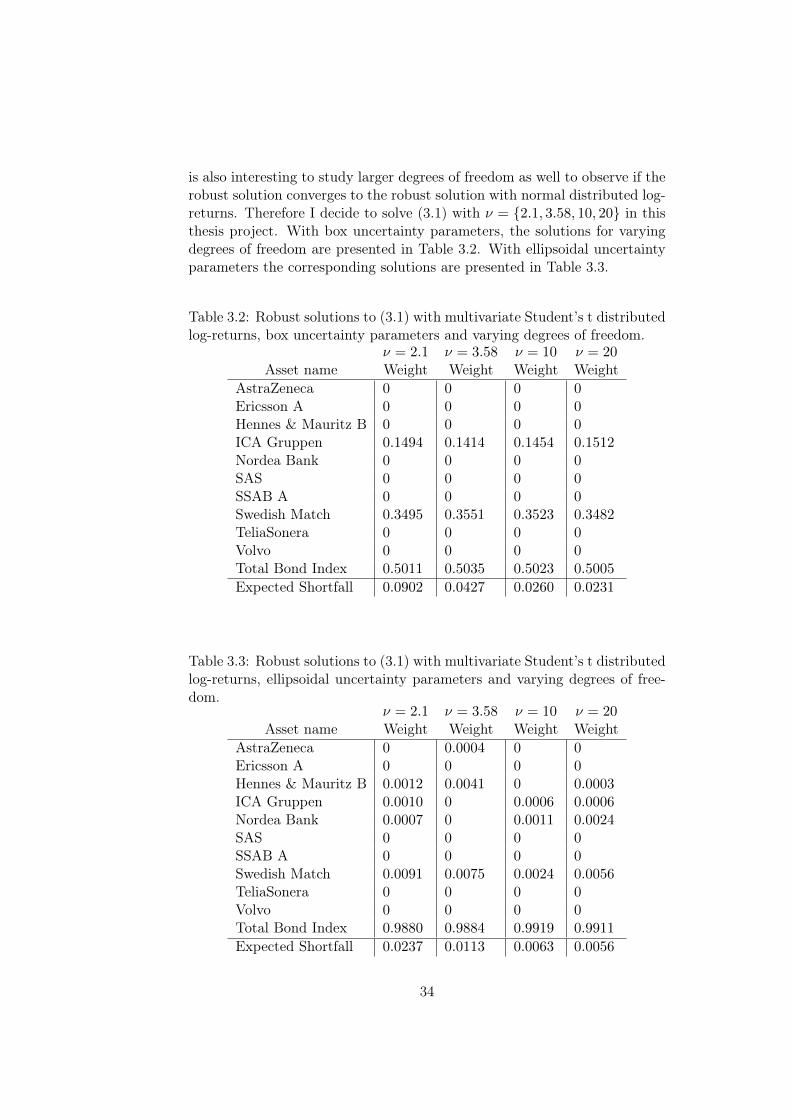
is also interesting to study larger degrees of freedom as well to observe if therobust solution converges to the robust solution with normal distributed log-returns. Therefore I decide to solve (3.1) with ν = {2.1, 3.58, 10, 20} in thisthesis project. With box uncertainty parameters, the solutions for varyingdegrees of freedom are presented in Table 3.2. With ellipsoidal uncertaintyparameters the corresponding solutions are presented in Table 3.3.

Table 3.2: Robust solutions to (3.1) with multivariate Student’s t distributedlog-returns, box uncertainty parameters and varying degrees of freedom.

ν = 2.1 ν = 3.58 ν = 10 ν = 20Asset name Weight Weight Weight Weight

AstraZeneca 0 0 0 0Ericsson A 0 0 0 0Hennes & Mauritz B 0 0 0 0ICA Gruppen 0.1494 0.1414 0.1454 0.1512Nordea Bank 0 0 0 0SAS 0 0 0 0SSAB A 0 0 0 0Swedish Match 0.3495 0.3551 0.3523 0.3482TeliaSonera 0 0 0 0Volvo 0 0 0 0Total Bond Index 0.5011 0.5035 0.5023 0.5005

Expected Shortfall 0.0902 0.0427 0.0260 0.0231

Table 3.3: Robust solutions to (3.1) with multivariate Student’s t distributedlog-returns, ellipsoidal uncertainty parameters and varying degrees of free-dom.

ν = 2.1 ν = 3.58 ν = 10 ν = 20Asset name Weight Weight Weight Weight

AstraZeneca 0 0.0004 0 0Ericsson A 0 0 0 0Hennes & Mauritz B 0.0012 0.0041 0 0.0003ICA Gruppen 0.0010 0 0.0006 0.0006Nordea Bank 0.0007 0 0.0011 0.0024SAS 0 0 0 0SSAB A 0 0 0 0Swedish Match 0.0091 0.0075 0.0024 0.0056TeliaSonera 0 0 0 0Volvo 0 0 0 0Total Bond Index 0.9880 0.9884 0.9919 0.9911

Expected Shortfall 0.0237 0.0113 0.0063 0.0056

34

Similarly to the case with normal distributed log-returns, to avoid intro-ducing statistical uncertainty in the solutions, it is possible to solve Markowitzmean-variance optimization problem (1.3) with the same worst-case parame-ters and risk aversion coefficient c calculated using (2.11) with the Student’st quantile function. Those solutions are presented in Appendix C.2 as refer-ence solutions to validate the accuracy of the simulated solutions.

3.1.3 Robust Optimization with Asymmetric Distributions

A well known problem when fitting distributions to empirical data withMaximum-Likelihood estimation is that most focus is on fitting the center ofthe distribution and less focus is on the tails. This is because by definitionmore observations are located in the center than in the tails of the empiricaldistribution. This behavior is unfortunate when calculating risk measuressuch as Expected Shortfall which depends heavily on the loss tail of themodeled distribution. One attempt to solve this problem is to model thedistributional tails and center separately.

3.1.3.1 The univariate generalized Pareto distribution

Modeling the tails and center of a univariate empirical distribution sepa-rately results in an asymmetric log-return distribution and there is no longera simple analytical relationship between Markowitz mean-variance optimiza-tion problem and the portfolio optimization problem with Expected Short-fall. This is of course of interest because then problem formulation (2.7) isa unique portfolio optimization problem not identical to a Markowitz mean-variance optimization problem.

A distribution that is popular to use for modeling the tails of an empiricallog-return distribution is the generalized Pareto distribution (GPD). Morecorrectly, given independent and identically distributed residuals r1, . . . , rnwith unknown distribution function F and a high threshold uh, the excessesrk − uh often turns out to be well modeled by the generalized Pareto dis-tribution. For a shape parameter γ > 0 and a scale parameter β > 0, thegeneralized Pareto distribution is given by

Gγ,β(x) = 1−(

1 +γx

β

)− 1γ

, x ≥ 0

and for γ = 0 it is given by

Gγ,β(x) = 1− e−xβ , x ≥ 0.

The choice of a suitably high threshold uh is crucial, but often hard,for the generalized Pareto distribution to be a good fit to the excesses. Ifuh is too large then few observations can be used for parameter estimation

35

yielding poor estimates with large variation. If instead uh is too small thenmore observations can be used to estimate the parameters but modelingthe excesses with the generalized Pareto distribution becomes questionable.One approach to estimate the parameters is to pick some uh1 far out in theempirical distribution, say the 90% quantile of the empirical distribution,and estimate the parameters with Maximum Likelihood estimation. Then anew threshold uh2 is chosen farther out in the empirical distribution, say the91% quantile, and the parameters are estimated once again with MaximumLikelihood estimation. The procedure is repeated and the threshold uh ischosen as the first candidate for which the parameters to the generalizedPareto distribution are stable from that point on. This method relies on theassumption that the parameters will converge before we are not too far outin the distribution tail. With data originating from the historical log-returnsin this thesis project the method could not be used because the parametersdid not converge until very far out in the distribution tail. Instead, thethreshold were chosen as the 90% empirical quantile, i.e. uh = F−1

n (0.90),for each asset in the reference portfolio1. In Section 4.3 I mention anotherstrategy that could be used to choose better values of uh.

Note that the generalized Pareto distribution models excesses above ahigh threshold uh which means that we are looking at the upper tail of thelog-return distribution, but Expected Shortfall only depends on the lowertail of the log-return distribution. Luckily, if the lower tail of the log-returndistribution consists solely of negative values below some negative thresholdul one may simply look at the absolute values and the "excess" of an ob-servation in the lower tail is then the positive distance from the observationto ul and one can model the lower tail of the log-return distribution with ageneralized Pareto distribution as well. Levine makes use of this strategy in[9] when modeling the lower tail of the total monthly return distribution forthe A-rated 7- to 10-year corporate bond component of Citi’s U.S. Broad In-vestment Grade Bond Index from January 1980 to August 2008. Similarly tothe upper threshold uh, the lower thresholds are chosen as the 10% empiricalquantile, i.e. ul = F−1

n (0.10), for each asset in the reference portfolio.Since generalized Pareto distributions can only be used to model the tails

of a distribution a third distribution must be used as a bridge to connect thetwo tails with the center of the distribution. In this thesis project, this isdone with the empirical distribution.

A mathematical expression for the entire underlying distribution willbe derived by considering two scenarios and then combining them. Considerfirst the scenario where the excesses above some threshold uh of a distributionconsisting of independent and identically distributed random variables ismodeled with a generalized Pareto distribution Ghγ,β(x − uh). For x ≥ uh

1Skoglund and Nyström show in [13] that Maximum Likelihood estimation of general-ized Pareto distribution parameters is not sensitive of the choice of threshold value.

36

the cumulative distribution function of the underlying distribution is givenby

P (X ≤ x) = P (X ≤ uh) + P (uh ≤ X ≤ x)

= P (X ≤ uh) + (1− P (X ≤ uh))Ghγ,β(x− uh).

The probability P (X ≤ uh) is estimated by the empirical distribution func-tion as P (X ≤ uh) ≈ Fn(uh). For x < uh the remaining underlying dis-tribution is modeled with the empirical distribution Fn(x). The cumulativedistribution function for the entire underlying distribution is then modeledas

F (x) =

{Fn(x), x < uh

Fn(uh) + (1− Fn(uh))Ghγ,β(x− uh), x ≥ uh.

Now consider the reversed scenario where the "excesses" of the independentand identically distributed random variables below some threshold ul is mod-eled by a generalized Pareto distribution Glγ,β(ul − x) and for x > ul theremaining underlying distribution is modeled with the empirical distribu-tion Fn(x). The cumulative distribution function for the entire underlyingdistribution is in this case modeled as

F (x) =

{Fn(ul)

(1−Glγ,β(ul − x)

), x ≤ ul

Fn(x), x > ul.

By combining the two scenarios, the cumulative distribution function for theentire underlying distribution is given by

F (x) =

Fn(ul)

(1−Glγ,β(ul − x)

), x ≤ ul

Fn(x), ul < x < uh

Fn(uh) + (1− Fn(uh))Ghγ,β(x− uh), x ≥ uh.(3.7)

where the shape and scale parameters γ and β may differ between the twogeneralized Pareto distribution functions Glγ,β(x) and Ghγ,β(x). The cumula-tive distribution function (3.7) is asymmetric and will be referred to in thisthesis project as the hybrid GPD-Empirical-GPD distribution.

3.1.3.2 Copula dependence

The generalized Pareto distribution is univariate so for each asset in the refer-ence portfolio two unique generalized Pareto distributions and the empiricaldistribution must be modeled to obtain unique univariate cumulative distri-bution functions. To capture the dependence between the different assets acopula may be used. A copula can be explained as a function that couples ajoint distribution function to univariate marginal distribution functions andit is from the joint distribution function where the multivariate dependence

37

between the univariate random variables is inherited. A copula is constructedby combining probability and quantile transforms. If X is a random variablewith continuous distribution function F then the probability transform statesthat F (X) has uniform distribution on (0, 1), i.e. F (X) is U(0, 1). If U is arandom variable with uniform distribution on (0, 1) and G is some distribu-tion function then the quantile transform states thatG−1(U) has distributionfunction G, i.e. P (G−1(U) ≤ x) = G(x). Using the probability transform itfollows that for a random vector U = (U1, . . . , Un) whose components haveuniform distribution on (0, 1) a random vector X = (X1, . . . , Xn) whosecomponents have marginal distributions F1, . . . , Fn can be constructed as

X = (F−11 (U1), . . . , F−1

n (Un)). (3.8)

Now, to describe the dependence between the components of X one mayinstead describe the dependence between the components of U and use (3.8).The distribution function C(u1, . . . , un) is called a copula and using thequantile transform it follows that

C(F1(x1), . . . , Fn(xn)) = P (U1 ≤ F1(x1), . . . , Un ≤ Fn(xn)

= P (F−11 (U1) ≤ x1, . . . , F

−1n (Un) ≤ xn)

= F (x1, . . . , xn)

where F is the joint multivariate distribution of X.Since the components of U are transformed to components in X using

the marginal distributions of X it is important to realize that the measure ofdependence between the random variables must be invariant to this transfor-mation. Ordinary linear correlation is not invariant to this transformationwhich makes it necessary to find such a measure. One measure that hasthe desired property is the rank correlation Kendall’s tau. Kendall’s tau isdefined on the random vector (X1, X2) as

τ(X1, X2) = P((X1 −X ′1)(X2 −X ′2) > 0

)− P

((X1 −X ′1)(X2 −X ′2) < 0

)where (X ′1, X

′2) is an independent copy of (X1, X2). Lindskog, McNeil and

Schmock show in [10] that if (X1, X2) have an elliptical distribution then therelationship

τ(X1, X2) =2

πarcsin(ρ) (3.9)

holds under some technical conditions. The relationship makes it easy toconvert the linear correlation matrix C into a transformation invariant rankcorrelation matrix Cτ that can be used when simulating from an ellipticalcopula.

3.1.3.3 Sample Preparation with GARCH(1,1) Model

The validity of fitting a generalized Pareto distribution to excesses in a dis-tribution tail relies heavily on the assumption of independent and identically

38

distributed random variables. Hence, to model the tails of the empirical dis-tributions to each asset in the reference portfolio with generalized Paretodistribution it is of great importance that the data has the right properties.When initially defining log-returns in (1.1) it was mentioned that log-returnsare often assumed to be weakly dependent and close to independent andidentically distributed. In financial time series analysis of risk factors (herethe log-returns), stylized facts are effects that are commonly observed in thedata. Josefsson summarizes the stylized facts in [7] as

1. Return series are not independent and identically distributed althoughthey show little serial correlation.

2. Series of absolute or squared returns show significant serial correlation.

3. Conditional expected returns are close to zero.

4. Volatility appears to vary over time.

5. Return series are leptokurtic2 or heavy tailed.

6. Extreme returns appear in clusters.

The stylized facts are problematic since they imply that the empirical log-returns cannot be considered independent and identically distributed andhence the excesses in the distribution tails cannot be modeled directly withgeneralized Pareto distributions. Some sample preparation has to be done,typically by filtering the data through a time series model. A popular modelused for filtering financial log-return data is the Generalized AutoregressiveConditional Heteroscedasticity, GARCH, model.

The general GARCH(p,q) process is defined in the following way. Let{Zt} be independent and identically distributed N(0, 1). Then {Xt} is calleda GARCH(p,q) process if

Xt = µ+ σtZt, t ∈ Z

where {σt} is the nonnegative process

σ2t = α0 +

p∑i=1

αiX2t−i +

q∑j=1

βjσ2t−j ,

and α0 > 0, αj , βj ≥ 0, j = 1, 2, . . . . For more on GARCH(p,q) processesand other time series models I refer to [1] by Brockwell and Davis. Notefrom the GARCH model that if Xt is interpreted as the log-return at timet then the model is a linear combination of squared historical log-returns

2A leptokurtic distribution has fatter tails and higher peak than the curvature foundin a normal distribution.

39

which fits stylized fact 2. Also, the volatility is dependent on time and onprevious volatilities, which fits stylized facts 4 and 6. This is an intuitivemotivation on why GARCH models often fits historical log-return time serieswell. Furthermore, by applying Hölder’s inequality when calculating thekurtosis of σtZt,

k(σtZt) =E[(σtZt)

4]

E[(σtZt)2]2= k(Zt)

E[σ4t ]

E[σ2t ]

2≥ k(Zt)

it is seen that it is greater than the kurtosis of Zt. Hence, even thoughthe residuals are assumed to be normal distributed, the GARCH(p,q) modeltakes into account that log-returns often have fatter tails than the normaldistribution. This fits well with stylized fact 5.

There are methods for fitting general GARCH(p,q) models to time seriesdata which require us to find p, q, α0, . . . , αp, β1, . . . , βq. In this thesis projectI settle with fitting GARCH(1,1) models to the historical log-returns, whichmakes the process easier. GARCH(1,1) models are used since they are oftengood enough to filter financial data and the parameters can for instance beapproximated by Maximum Likelihood estimation.

When the parameters have been estimated the standardized residuals{Zt} are obtained as

Zt =Rt − µσt

and if the GARCH filtration is successful then the stylized facts should be ac-counted for, meaning that the standardized residuals should be independentand identically distributed.

In Appendix D I analyze the standardized residuals to the filtered empir-ical log-returns and conclude that the distribution tails are asymmetric andheavier than for the standard normal distribution assumed in the definitionof the GARCH process. In practice this is not a problem since the standard-ized residuals can be modeled by any suitable distribution. This motivatesthe idea of modeling the tails with generalized Pareto distributions.

3.1.3.4 Solution with Normal Copula and Hybrid GPD-Empirical-GPD Log-return Marginals

In this section I solve the robust portfolio optimization problem (3.1) withworst-case scenario parameters originating from both box and ellipsoidaluncertainty sets and log-returns simulated from a normal copula with hy-brid GPD-Empirical-GPD marginal distributions. Skoglund and Wei notein [19, p. 132] that the choice of copula has a second-order effect whenmodeling market risk factors such as stock log-returns, the most importantfactor being to model stochastic volatility and volatility clustering which isaccounted for in the GARCH(p,q) model. Hence choosing the normal copulafor dependency structure is not the most important decision in the modeling

40

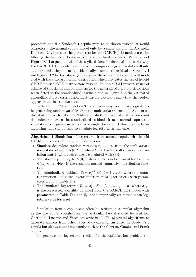
procedure and if a Student’s t copula were to be chosen instead, it wouldoutperform the normal copula model only by a small margin. In AppendixD, Table D.1, I present the parameters for the GARCH(1,1) models used forfiltering the historical log-returns to standardized residuals. With help ofFigure D.1 I argue on basis of the stylized facts for financial time series whythe GARCH(1,1) models have filtered the empirical log-return data well intostandardized independent and identically distributed residuals. Secondly Iuse Figure D.2 to describe why the standardized residuals are not well mod-eled with the standard normal distribution which motivates the use of hybridGPD-Empirical-GPD distributions instead. In Table D.2 I present values ofestimated thresholds and parameters for the generalized Pareto distributionswhen fitted to the standardized residuals and in Figure D.3 the estimatedgeneralized Pareto distribution functions are plotted to show that the modelsapproximate the true data well.

In Section 3.1.2.1 and Section 3.1.2.2 it was easy to simulate log-returnsby generating random variables from the multivariate normal and Student’s tdistribution. With hybrid GPD-Empirical-GPD marginal distributions anddependence between the standardized residuals from a normal copula thesimulation of log-returns is not as straight forward. Below I provide analgorithm that can be used to simulate log-returns in this case.

Algorithm 1 Simulation of log-returns from normal copula with hybridGPD-Empirical-GPD marginal distributions1: Simulate dependent random variables x1, . . . , xn from the multivariate

normal distribution N(0, Cτ ), where Cτ is the Kendall’s tau rank corre-lation matrix with each element calculated with (3.9).

2: Transform x1, . . . , xn to U(0, 1) distributed random variables as ui =Φ(xi) where Φ(x) is the standard normal cumulative distribution func-tion.

3: The standardized residuals Zi = F−1i (ui), i = 1, . . . , n, where the quan-

tile function F−1i is the inverse function of (3.7) for asset i with param-

eters found in Table D.2.4: The simulated log-returns Ri = σit+1Zi + µi, i = 1, . . . , n, where σit+1

is the forecasted volatility obtained from the GARCH(1,1) model withparameters in Table D.1 and µi is the empirically estimated mean log-return value for asset i.

Simulation from a copula can often be written in a similar algorithmas the one above, specified for the particular task it should be used for.Cherubini, Luciano and Vecchiato write in [2, Ch. 6] several algorithms togenerate samples from other types of copulas, for instance the Student’s tcopula but also archimedean copulas such as the Clayton, Gumbel and Frankcopula.

To generate the log-returns needed for the optimization problem the

41

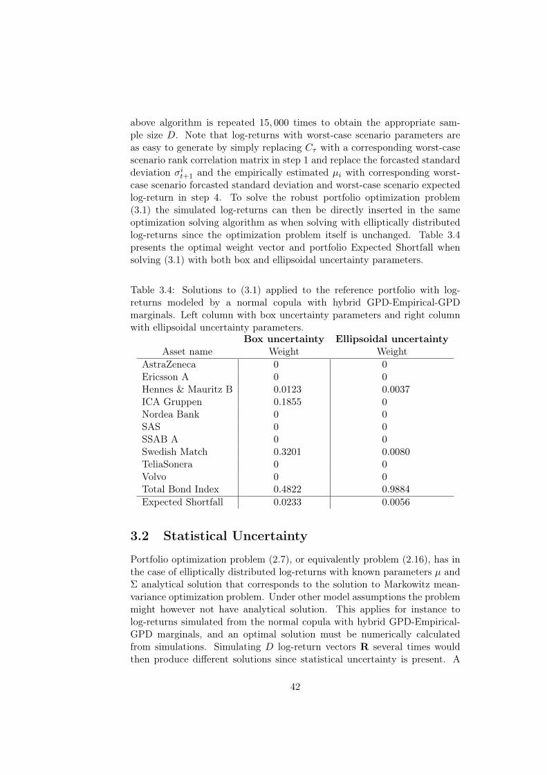
above algorithm is repeated 15, 000 times to obtain the appropriate sam-ple size D. Note that log-returns with worst-case scenario parameters areas easy to generate by simply replacing Cτ with a corresponding worst-casescenario rank correlation matrix in step 1 and replace the forcasted standarddeviation σit+1 and the empirically estimated µi with corresponding worst-case scenario forcasted standard deviation and worst-case scenario expectedlog-return in step 4. To solve the robust portfolio optimization problem(3.1) the simulated log-returns can then be directly inserted in the sameoptimization solving algorithm as when solving with elliptically distributedlog-returns since the optimization problem itself is unchanged. Table 3.4presents the optimal weight vector and portfolio Expected Shortfall whensolving (3.1) with both box and ellipsoidal uncertainty parameters.

Table 3.4: Solutions to (3.1) applied to the reference portfolio with log-returns modeled by a normal copula with hybrid GPD-Empirical-GPDmarginals. Left column with box uncertainty parameters and right columnwith ellipsoidal uncertainty parameters.

Box uncertainty Ellipsoidal uncertaintyAsset name Weight Weight

AstraZeneca 0 0Ericsson A 0 0Hennes & Mauritz B 0.0123 0.0037ICA Gruppen 0.1855 0Nordea Bank 0 0SAS 0 0SSAB A 0 0Swedish Match 0.3201 0.0080TeliaSonera 0 0Volvo 0 0Total Bond Index 0.4822 0.9884

Expected Shortfall 0.0233 0.0056

3.2 Statistical Uncertainty

Portfolio optimization problem (2.7), or equivalently problem (2.16), has inthe case of elliptically distributed log-returns with known parameters µ andΣ analytical solution that corresponds to the solution to Markowitz mean-variance optimization problem. Under other model assumptions the problemmight however not have analytical solution. This applies for instance tolog-returns simulated from the normal copula with hybrid GPD-Empirical-GPD marginals, and an optimal solution must be numerically calculatedfrom simulations. Simulating D log-return vectors R several times wouldthen produce different solutions since statistical uncertainty is present. A

42

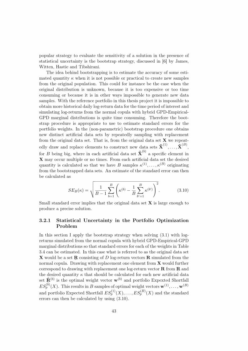
popular strategy to evaluate the sensitivity of a solution in the presence ofstatistical uncertainty is the bootstrap strategy, discussed in [6] by James,Witten, Hastie and Tibshirani.

The idea behind bootstrapping is to estimate the accuracy of some esti-mated quantity κ when it is not possible or practical to create new samplesfrom the original population. This could for instance be the case when theoriginal distribution is unknown, because it is too expensive or too timeconsuming or because it is in other ways impossible to generate new datasamples. With the reference portfolio in this thesis project it is impossible toobtain more historical daily log-return data for the time period of interest andsimulating log-returns from the normal copula with hybrid GPD-Empirical-GPD marginal distributions is quite time consuming. Therefore the boot-strap procedure is appropriate to use to estimate standard errors for theportfolio weights. In the (non-parametric) bootstrap procedure one obtainsnew distinct artificial data sets by repeatedly sampling with replacementfrom the original data set. That is, from the original data set X we repeat-edly draw and replace elements to construct new data sets X

(1), . . . , X

(B),

for B being big, where in each artificial data set X(b)

a specific element inX may occur multiple or no times. From each artificial data set the desiredquantity is calculated so that we have B samples κ(1), . . . , κ(B) originatingfrom the bootstrapped data sets. An estimate of the standard error can thenbe calculated as

SEB(κ) =

√√√√ 1

B − 1

B∑b=1

(κ(b) − 1

B

B∑b′=1

κ(b′)

)2

. (3.10)

Small standard error implies that the original data set X is large enough toproduce a precise solution.

3.2.1 Statistical Uncertainty in the Portfolio OptimizationProblem

In this section I apply the bootstrap strategy when solving (3.1) with log-returns simulated from the normal copula with hybrid GPD-Empirical-GPDmarginal distributions so that standard errors for each of the weights in Table3.4 can be estimated. In this case what is referred to as the original data setX would be a set

¯R consisting of D log-return vectors R simulated from the

normal copula. Drawing with replacement one element fromX would furthercorrespond to drawing with replacement one log-return vector R from

¯R and

the desired quantity κ that should be calculated for each new artificial dataset

¯R(b) is the optimal weight vector w(b) and portfolio Expexted Shortfall

ES(b)p (X). This results in B samples of optimal weight vectorsw(1), . . . ,w(B)

and portfolio Expected Shortfall ES(1)p (X), . . . , ES

(B)p (X) and the standard

errors can then be calculated by using (3.10).

43

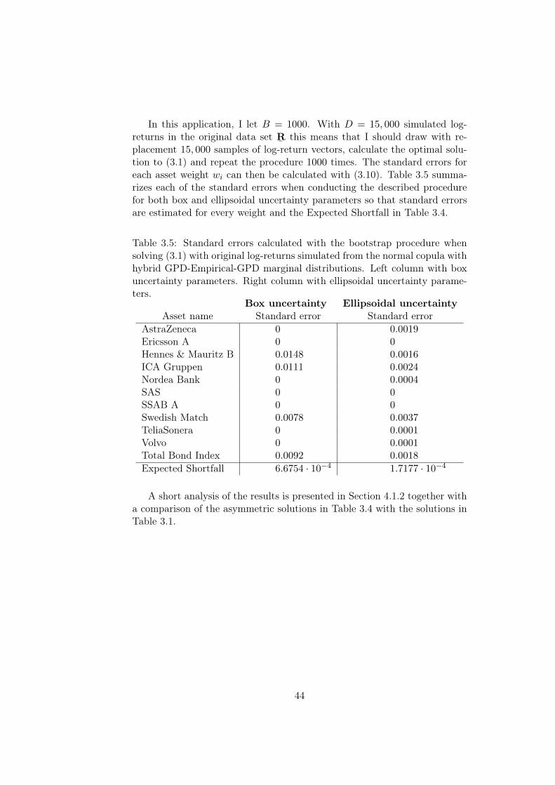
In this application, I let B = 1000. With D = 15, 000 simulated log-returns in the original data set

¯R this means that I should draw with re-

placement 15, 000 samples of log-return vectors, calculate the optimal solu-tion to (3.1) and repeat the procedure 1000 times. The standard errors foreach asset weight wi can then be calculated with (3.10). Table 3.5 summa-rizes each of the standard errors when conducting the described procedurefor both box and ellipsoidal uncertainty parameters so that standard errorsare estimated for every weight and the Expected Shortfall in Table 3.4.

Table 3.5: Standard errors calculated with the bootstrap procedure whensolving (3.1) with original log-returns simulated from the normal copula withhybrid GPD-Empirical-GPD marginal distributions. Left column with boxuncertainty parameters. Right column with ellipsoidal uncertainty parame-ters.

Box uncertainty Ellipsoidal uncertaintyAsset name Standard error Standard error

AstraZeneca 0 0.0019Ericsson A 0 0Hennes & Mauritz B 0.0148 0.0016ICA Gruppen 0.0111 0.0024Nordea Bank 0 0.0004SAS 0 0SSAB A 0 0Swedish Match 0.0078 0.0037TeliaSonera 0 0.0001Volvo 0 0.0001Total Bond Index 0.0092 0.0018

Expected Shortfall 6.6754 · 10−4 1.7177 · 10−4

A short analysis of the results is presented in Section 4.1.2 together witha comparison of the asymmetric solutions in Table 3.4 with the solutions inTable 3.1.

44

Chapter 4

Analysis and Conclusions

In this chapter the results found in the previous chapter are analyzed. Ialso give comments on the interpretation of robust optimization as worst-case scenario based optimization. The thesis project ends with comments onalternative approaches that could have been made and comments on areasof further investigation is mentioned.

4.1 Analysis of Results

In this section the results obtained throughout the thesis project are analyzedand compared to gain knowledge of how the different model assumptionsinvestigated affect the optimal solution to the robust portfolio optimizationproblem with Expected Shortfall.

An initial observation valid for all solutions is that even though 11 assetsare included in the reference portfolio, only a few of them are actually in-vested in. This could initially be seen as counter-intuitive since the resultingportfolio would be more diversified if the initial capital were spread acrossmore assets and the investor could become exposed to less risk. The keyto understand this behavior is however to recall that with highly correlatedassets the idea of a well diversified portfolio lose its meaning. As an example,consider a portfolio consisting of two assets with correlation 1 but differentexpected log-returns. In that case the risk would not decrease if half the cap-ital were allocated in each of the assets since they are perfectly correlated.It would hence be better to invest everything in the asset with the higherexpected log-return. The same principle holds for the reference portfolio inthis thesis project and diversifying the initial capital more than suggested bythe optimal solution would decrease the expected portfolio log-return morethan the decrease in Expected Shortfall and make the solution sub-optimal.If a more distributed portfolio allocation is preferred by the investor thenadditional lower and upper bounds on the weights could be added to theportfolio optimization problem formulation. As an example, pension funds

45

often have restrictions on the portfolio weights in different asset classes andindustries.

4.1.1 Elliptically distributed log-returns

Here the different solutions with elliptically distributed log-returns will becompared and analyzed. More specifically, the benchmark solution in Ta-ble 1.2 and the solutions in Table 2.1 and Table 3.1 through Table (3.3)are investigated. Since portfolio optimization with Expected Shortfall isdirectly related to Markowitz mean-variance optimization with ellipticallydistributed log-returns I may compare the robust solutions to (2.16) to thebenchmark solution to analyze the effect of model uncertainty in portfoliooptimization.

The first observation that I make is that with box uncertainty parame-ters the robust solutions resembles the benchmark solution more than withellipsoidal uncertainty parameters. This is seen by observing that the solu-tions in the left columns of Table 3.1 and Table 3.2 have similar structure asthe benchmark solution in Table 1.2 while the solutions in the right columnsof Table 3.1 and Table 3.3 differs more from the benchmark solution. Withbox uncertainty parameters the initial capital is invested in the same as-sets as in the benchmark solution and the only difference is that the robustsolutions are a bit more diversified. With ellipsoidal uncertainty sets thewast majority of the initial capital is invested in the Total Bond Index andapproximately one percent of the capital is diversified across a few other as-sets. Note that this result dependents on how much µmin and Σmax deviatefrom the empirically estimated parameters where larger deviations lead tolarger solution deviation from the benchmark solution. I can therefore con-clude from the optimal solutions that the ellipsoidal uncertainty parametersdeviate more from the empirically estimated parameters than the box un-certainty parameters, which is confirmed by comparing the numerical valuesin Appendix A. The results from robust optimization with box uncertaintyparameters can be seen as a stress test of the optimization problem wherethe investor has a more conservative view on the market than the historicaldata suggests, while robust optimization with ellipsoidal uncertainty param-eters could be seen as exposing the portfolio optimization problem to a largefinancial crisis. A conclusion independent of the particular parameters usedin this thesis project is that portfolio optimization with Expected Shortfall issensitive to parameter uncertainty. This can be concluded since the robustoptimal solutions deviate notably from the benchmark solution regardlessof which worst-case scenario parameters that are used. If the optimizationproblem would had been insensitive to parameter uncertainty then the robustsolutions would have been close to each other and close to the benchmarksolution. It is therefore of great importance to take into consideration uncer-tainties in parameters when solving a portfolio optimization problem. Quite

46

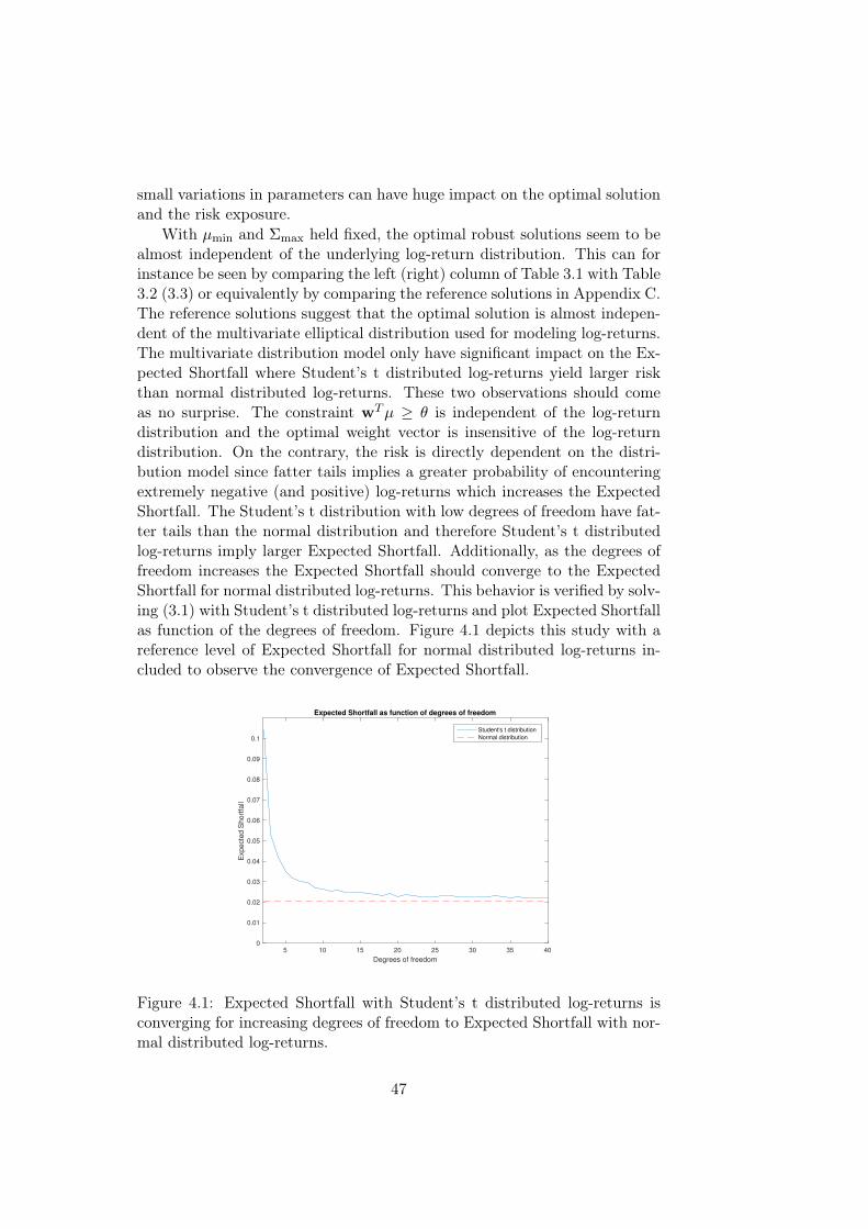
small variations in parameters can have huge impact on the optimal solutionand the risk exposure.

With µmin and Σmax held fixed, the optimal robust solutions seem to bealmost independent of the underlying log-return distribution. This can forinstance be seen by comparing the left (right) column of Table 3.1 with Table3.2 (3.3) or equivalently by comparing the reference solutions in Appendix C.The reference solutions suggest that the optimal solution is almost indepen-dent of the multivariate elliptical distribution used for modeling log-returns.The multivariate distribution model only have significant impact on the Ex-pected Shortfall where Student’s t distributed log-returns yield larger riskthan normal distributed log-returns. These two observations should comeas no surprise. The constraint wTµ ≥ θ is independent of the log-returndistribution and the optimal weight vector is insensitive of the log-returndistribution. On the contrary, the risk is directly dependent on the distri-bution model since fatter tails implies a greater probability of encounteringextremely negative (and positive) log-returns which increases the ExpectedShortfall. The Student’s t distribution with low degrees of freedom have fat-ter tails than the normal distribution and therefore Student’s t distributedlog-returns imply larger Expected Shortfall. Additionally, as the degrees offreedom increases the Expected Shortfall should converge to the ExpectedShortfall for normal distributed log-returns. This behavior is verified by solv-ing (3.1) with Student’s t distributed log-returns and plot Expected Shortfallas function of the degrees of freedom. Figure 4.1 depicts this study with areference level of Expected Shortfall for normal distributed log-returns in-cluded to observe the convergence of Expected Shortfall.

5 10 15 20 25 30 35 40

Degrees of freedom

0

0.01

0.02

0.03

0.04

0.05

0.06

0.07

0.08

0.09

0.1

Exp

ecte

d S

ho

rtfa

ll

Expected Shortfall as function of degrees of freedom

Student's t distribution

Normal distribution

Figure 4.1: Expected Shortfall with Student’s t distributed log-returns isconverging for increasing degrees of freedom to Expected Shortfall with nor-mal distributed log-returns.

47

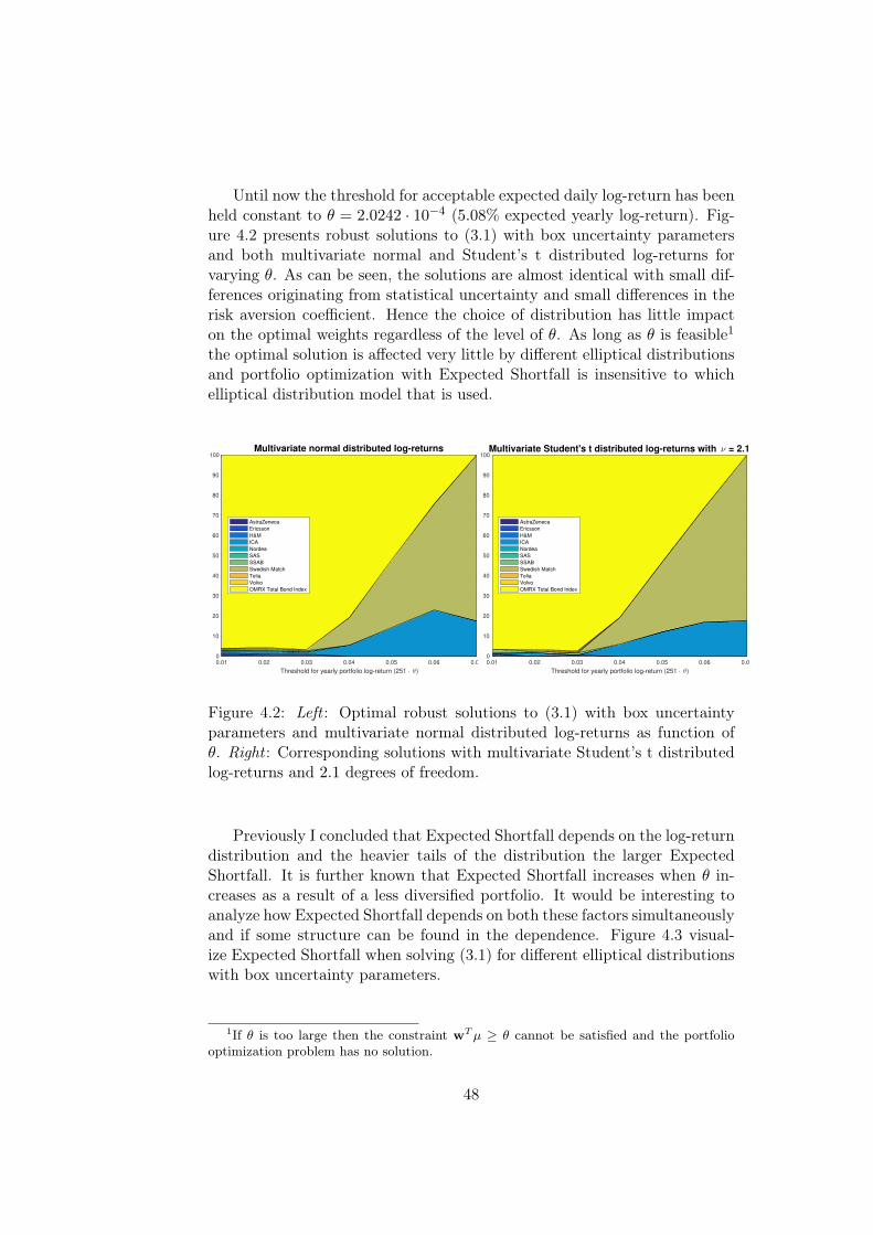
Until now the threshold for acceptable expected daily log-return has beenheld constant to θ = 2.0242 · 10−4 (5.08% expected yearly log-return). Fig-ure 4.2 presents robust solutions to (3.1) with box uncertainty parametersand both multivariate normal and Student’s t distributed log-returns forvarying θ. As can be seen, the solutions are almost identical with small dif-ferences originating from statistical uncertainty and small differences in therisk aversion coefficient. Hence the choice of distribution has little impacton the optimal weights regardless of the level of θ. As long as θ is feasible1

the optimal solution is affected very little by different elliptical distributionsand portfolio optimization with Expected Shortfall is insensitive to whichelliptical distribution model that is used.

0.01 0.02 0.03 0.04 0.05 0.06 0.07

Threshold for yearly portfolio log-return (251 · θ)

0

10

20

30

40

50

60

70

80

90

100

Op

tim

al a

sse

t w

eig

ht

wi i

n p

erc

en

t

Multivariate normal distributed log-returns

AstraZeneca

Ericsson

H&M

ICA

Nordea

SAS

SSAB

Swedish Match

Telia

Volvo

OMRX Total Bond Index

0.01 0.02 0.03 0.04 0.05 0.06 0.07

Threshold for yearly portfolio log-return (251 · θ)

0

10

20

30

40

50

60

70

80

90

100

Op

tim

al a

sse

t w

eig

ht

wi i

n p

erc

en

t

Multivariate Student's t distributed log-returns with ν = 2.1

AstraZeneca

Ericsson

H&M

ICA

Nordea

SAS

SSAB

Swedish Match

Telia

Volvo

OMRX Total Bond Index

Figure 4.2: Left : Optimal robust solutions to (3.1) with box uncertaintyparameters and multivariate normal distributed log-returns as function ofθ. Right : Corresponding solutions with multivariate Student’s t distributedlog-returns and 2.1 degrees of freedom.

Previously I concluded that Expected Shortfall depends on the log-returndistribution and the heavier tails of the distribution the larger ExpectedShortfall. It is further known that Expected Shortfall increases when θ in-creases as a result of a less diversified portfolio. It would be interesting toanalyze how Expected Shortfall depends on both these factors simultaneouslyand if some structure can be found in the dependence. Figure 4.3 visual-ize Expected Shortfall when solving (3.1) for different elliptical distributionswith box uncertainty parameters.

1If θ is too large then the constraint wTµ ≥ θ cannot be satisfied and the portfoliooptimization problem has no solution.

48

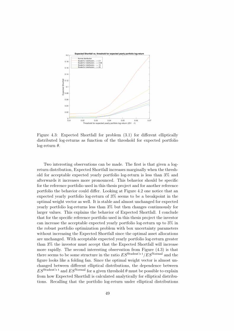
0.01 0.02 0.03 0.04 0.05 0.06 0.07

Threshold for expected yearly portfolio log-return (251 · θ)

0

0.02

0.04

0.06

0.08

0.1

0.12

0.14

0.16

0.18

0.2

Expecte

d S

hort

fall

Expected Shortfall vs. threshold for expected yearly portfolio log-return

Normal distribution

Student's t distribution, ν = 2.1

Student's t distribution, ν = 3.58

Student's t distribution, ν = 10

Student's t distribution, ν = 20

Figure 4.3: Expected Shortfall for problem (3.1) for different ellipticallydistributed log-returns as function of the threshold for expected portfoliolog-return θ.

Two interesting observations can be made. The first is that given a log-return distribution, Expected Shortfall increases marginally when the thresh-old for acceptable expected yearly portfolio log-return is less than 3% andafterwards it increases more pronounced. This behavior should be specificfor the reference portfolio used in this thesis project and for another referenceportfolio the behavior could differ. Looking at Figure 4.2 one notice that anexpected yearly portfolio log-return of 3% seems to be a breakpoint in theoptimal weight vector as well. It is stable and almost unchanged for expectedyearly portfolio log-returns less than 3% but then changes continuously forlarger values. This explains the behavior of Expected Shortfall. I concludethat for the specific reference portfolio used in this thesis project the investorcan increase the acceptable expected yearly portfolio log-return up to 3% inthe robust portfolio optimization problem with box uncertainty parameterswithout increasing the Expected Shortfall since the optimal asset allocationsare unchanged. With acceptable expected yearly portfolio log-return greaterthan 3% the investor must accept that the Expected Shortfall will increasemore rapidly. The second interesting observation from Figure (4.3) is thatthere seems to be some structure in the ratio ESStudent’s t/ESNormal and thefigure looks like a folding fan. Since the optimal weight vector is almost un-changed between different elliptical distributions, the dependence betweenESStudent’s t and ESNormal for a given threshold θ must be possible to explainfrom how Expected Shortfall is calculated analytically for elliptical distribu-tions. Recalling that the portfolio log-return under elliptical distributions

49

can be written as (2.10), the portfolio Expected Shortfall is

ESp(wTR) = −wTµ+

√wTΣwESp(WZ1), (4.1)

where WZ1 determines which standard elliptical distribution is used. Now,since w is almost unchanged between different elliptical distributions and theparameters µ and Σ are not dependent on the distribution, it is differencesin Expected Shortfall for standard elliptical distributions, ESp(WZ1), thatdetermines the ratio ESStudent’s t/ESNormal. The ratio should therefore beapproximately proportional to ESStandard Student’s t

p /ESStandard Normalp where

the numerator depends on the degrees of freedom.

4.1.2 Asymmetric Distributed Log-returns

I continue the analysis of the results by comparing the robust solutions be-tween asymmetric and elliptically distributed log-returns. This allows me toconclude what impact the implementation of portfolio optimization problem(2.7) in favor of Markowitz mean-variance optimization problem (1.3) has,since it can handle asymmetric distributions. If an asymmetric distributionmodel have visible impact on the optimal solution then I can conclude thatproblem (2.7) is important since it changes the investment strategy. Some-thing that was not achieved by altering between elliptical distributions.

First of all I give a short comment on the GARCH(1,1) filtering andgeneralized Pareto distribution fit to the log-return distribution tails. Whenmodeling historical log-returns, the stylized facts in Section 3.1.3.3 shouldbe accounted for in a good model. Modeling the log-returns directly withan elliptical distribution may take into account the heavy tailed behaviorof the log-returns if the multivariate Student’s t distribution is used, butfor instance volatility clustering and significant serial autocorrelation is notaccounted for explicitly. By filtering the log-returns with a GARCH(1,1)model, the heavy tailed behavior is captured, as well as volatility clusteringand serial correlation. Hence, more stylized facts are taken into considera-tion which should result in a better model. A GARCH(1,1) model togetherwith generalized Pareto distribution models in the tails to account for asym-metry is thus a much more accurate model than an elliptical distributionmodel. The optimization results when simulating log-returns from a normalcopula with hybrid GPD-Empirical-GPD marginals should therefore be morereliable than the results when simulating from elliptical distributions.

Since the log-returns are simulated from a normal copula, the robust so-lutions in Table 3.4 will be compared to the solutions in Table 3.1 wherethe log-returns have multivariate normal distribution. Comparing the ta-bles shows that with both box and ellipsoidal uncertainty parameters theExpected Shortfall is greater when simulating log-returns from the normalcopula. The result is expected. As has been discussed before, the multi-variate normal distribution has not fat enough tails to be good at model-

50

ing historical log-return tails and therefore the Expected Shortfall calculatedwith multivariate normal distribution will be smaller than the true ExpectedShortfall. Modeling the tails with generalized Pareto distributions solves thisproblem and the tails are better modeled with fatter tails which results inlarger Expected Shortfall. In this sense, the Expected Shortfall in Table 3.4should be thought of as closer to reality than the Expected Shortfall in Table3.1.

It is not only the Expected Shortfall that changes when simulating log-returns from a normal copula with asymmetric marginals instead of simu-lating from a multivariate normal distribution. The optimal asset weightschange notably as well, seen by comparing the solutions in Table 3.1 andTable 3.4. The general structure of the investments is very similar betweenthe tables, but quite large differences can be seen in the amount of capi-tal invested when comparing individual assets. This behavior was not seenwhen changing between elliptical distributions. It can for instance be seenthat with box uncertainty parameters a switch to simulating with the normalcopula results in an investment increase of approximately 4% in ICA Grup-pen and 1% in Hennes & Mauritz B and a decrease of approximately 3% inSwedish Match and 2% in the Total Bond Index. These can be significantchanges. For instance, if $1 million is invested then there is a shift of ad-ditional $40, 000 invested in ICA Gruppen. The optimal solutions with boxuncertainty parameters differ more than with ellipsoidal uncertainty param-eters but this is likely due to that with ellipsoidal uncertainty parameters theoptimal solution suggests that almost all initial capital should be investedin one asset and this decision cannot be changed much without violatingthe constraint wTµ ≥ θ. In Section 4.1.3 I make an attempt to explain thedifferences in optimal solution by considering changes in each asset’s riskcontribution to the entire portfolio’s Expected Shortfall.

With elliptically distributed log-returns the optimal solutions to (3.1)could be compared to the analytical solutions in Appendix C where (1.3) issolved with risk aversion coefficient calculated by (2.11) to find an appropri-ate sample size. In that case it was concluded that with D = 15, 000 log-return samples the simulated solutions are close to the analytical solutions.With hybrid GPD-Empirical-GPD distributed log-returns the solutions can-not be compared with analytical solutions. Instead, standard errors to theoptimal solutions in Table 3.4 were calculated using the bootstrap methodwith results presented in Table 3.5. I begin by analyzing the solutions whenbox uncertainty parameters were used. By comparing the magnitudes of thestandard errors with the magnitudes of the asset weights I see that mostuncertainty lies in the Hennes & Mauritz B investment. The standard erroris larger than the investment and the true optimal weight might differ quitemuch from the one suggested and it is not possible to reject at a 95% con-fidence level that the true optimal investment is zero. In this sense, largersample size D of log-returns is desired to lower the standard error of the

51

optimal weight on that particular asset. On the other hand, the portfo-lio Expected Shortfall has very small standard error so the uncertainty inthe Hennes & Mauritz B investment seems to have little influence on theuncertainty in Expected Shortfall. In this sense larger sample size seemsunnecessary. I conclude that solving (3.1) with 15, 000 log-return samplessimulated from a normal copula with hybrid GPD-Empirical-GPD marginaldistributions yields acceptable accuracy, but increasing the sample size a bitfurther could increase the accuracy in the Hennes & Mauritz B investmentif this is important to the investor.

When it comes to the results in the right columns of Table 3.4 and 3.5where ellipsoidal uncertainty parameters have been used, the standard errorspoints out that it is not possible to reject that the true optimal weights forHennes & Mauritz B and Swedish Match are zero. This means that theoptimal solution with ellipsoidal uncertainty parameters could be to investeverything in the Total Bond Index. The result is easily interpreted. Withlarge volatility and correlations and small expected log-returns on the riskyassets in a portfolio, a conservative investor would, if he is forced to invest,invest all his capital in the least risky asset, being the Total Bond Index. Thestandard error for the portfolio Expected Shortfall is furthermore small andI conclude that with ellipsoidal uncertainty parameters, 15, 000 log-returnsamples simulated from a normal copula with hybrid GPD-Empirical-GPDmarginal distributions is large enough to obtain accurate solutions regardlessof which parameters are used.

In Section 4.1.1 I concluded that portfolio optimization with ExpectedShortfall is sensitive to uncertainties in the parameters µ and Σ. Now, af-ter analyzing the optimal robust solutions with different types of log-returndistribution models, I will extend the general conclusion and say somethingabout sensitivity to distribution. It has already been seen that the optimalweight vector is quite insensitive to different elliptical log-return distribu-tions. However, changing from an elliptical to an asymmetric distributionchanges the optimal weight vector significantly. I therefore conclude thatportfolio optimization with Expected Shortfall is sensitive to distributionuncertainty - if both elliptical and asymmetric distributions are included inthe distribution uncertainty set F . This is an interesting conclusions sincethe robust optimization community has not put much focus on distributionuncertainty. I can thus conclude that problem (2.7) indeed is important sincenot only parameter uncertainty but also distribution uncertainty affects theoptimal solution.

The major drawback with simulating log-returns from a normal copulawith hybrid GPD-Empirical-GPD marginal distributions is that the investoris required to use an algorithm such as Algorithm 1. The algorithm is po-tentially more time consuming than simulating log-returns from a simplemultivariate elliptical distribution since the data must be treated in foursteps rather than just one. With many risk factors the additional steps 2-

52

4 in Algorithm 1 can potentially take relatively long time. Therefore, thisapproach requires careful implementation for high frequency trading opti-mization but works perfectly fine in this application when trades are madeonce a day and can be used in favor of the simpler multivariate distributionapproach. The reasoning can be taken further and it can be concluded thatif it is of great importance to model the log-returns well, then portfolio opti-mization with Expected Shortfall is appropriate to use since the log-returnscan be modeled by copulas with different marginal distributions. The costis that the optimization problem becomes computationally heavier, is moretime consuming and introduces statistical uncertainty since simulations hasto be made. If a fast optimization procedure is important then Markowitzmean-variance optimization problem might be better to consider. An ex-ception is if the reference portfolio includes non-linear assets where portfoliooptimization with Expected Shortfall must be used or the assets must beapproximated by linear functions.

4.1.3 Analysis of Solutions with Euler Risk Decomposition

Up to this point I have motivated the appearance of the optimal weightvectors on basis of the expected log-return and volatility of each asset. Posi-tive expected log-return and small volatility should make an asset attractive,but with ellipsoidal uncertainty parameters, the optimal weight vector sug-gests to invest a small part of the capital in assets with negative expectedlog-return. In an attempt to explain this behavior, I will analyze the EulerAllocations defined in section 2.1.3 together with the expected log-returnvector, having the marginal Sharpe ratio (2.9) in mind.

In this thesis project, all financial instruments are linear assets, i.e.Fj(S(t)) = Sj(t) meaning that the sensitivities U = w and the Euler Allo-cation defined in (2.3) for normal distributed log-returns is simplified to

∂ESp(X)

∂U=∂ESp(X)

∂w= λ(Φ−1(q))(wTΣw)−1/2Σw

Table 4.1 presents robust Euler Allocations in the case where w is solvedwith box uncertainty parameters. The table also includes µ(box)

min on yearlybasis in percentage to make the analysis more convenient. For ellipsoidaluncertainty parameters, the corresponding Euler Allocations are presentedin Table 4.2. Recall that the optimal weight vectors are given in Table 3.1.

53

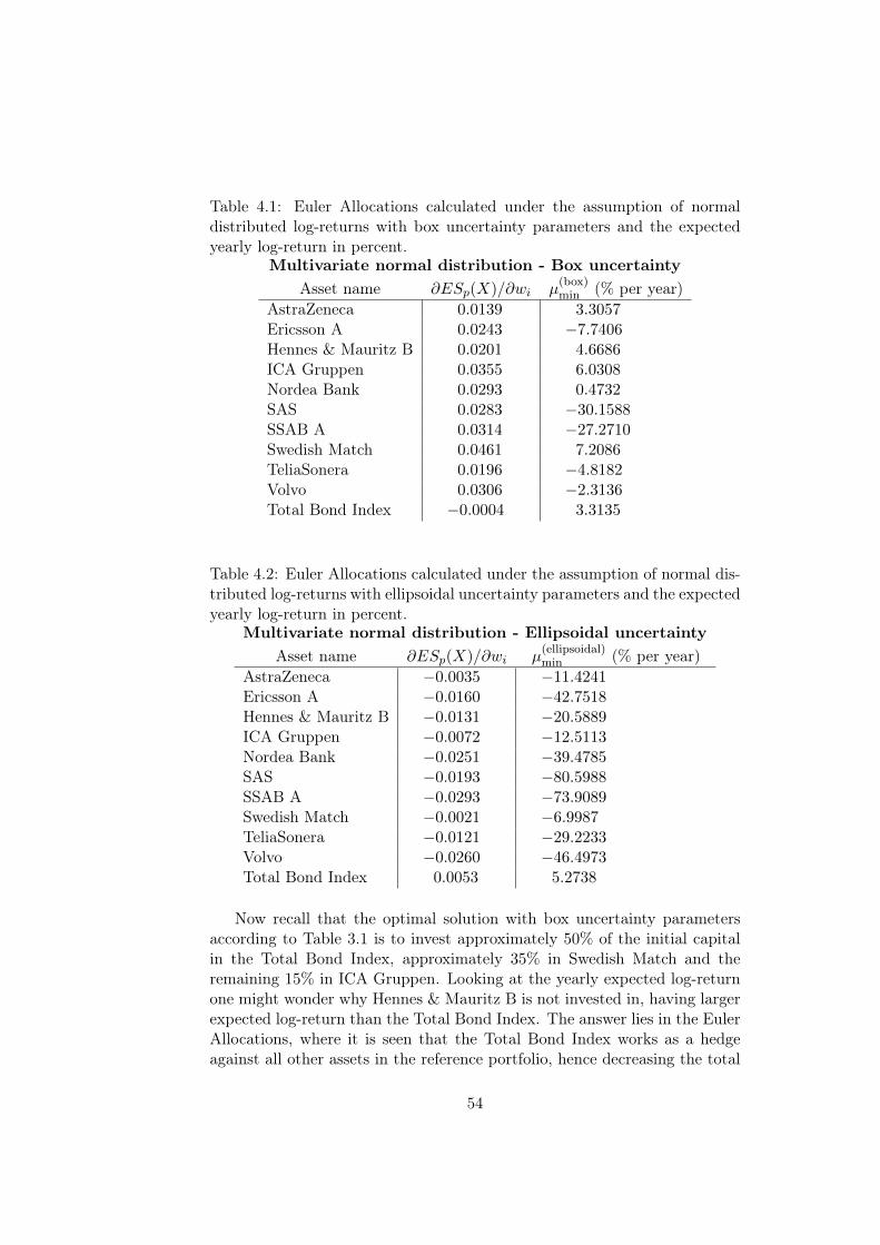
Table 4.1: Euler Allocations calculated under the assumption of normaldistributed log-returns with box uncertainty parameters and the expectedyearly log-return in percent.

Multivariate normal distribution - Box uncertaintyAsset name ∂ESp(X)/∂wi µ

(box)min (% per year)

AstraZeneca 0.0139 3.3057Ericsson A 0.0243 −7.7406Hennes & Mauritz B 0.0201 4.6686ICA Gruppen 0.0355 6.0308Nordea Bank 0.0293 0.4732SAS 0.0283 −30.1588SSAB A 0.0314 −27.2710Swedish Match 0.0461 7.2086TeliaSonera 0.0196 −4.8182Volvo 0.0306 −2.3136Total Bond Index −0.0004 3.3135

Table 4.2: Euler Allocations calculated under the assumption of normal dis-tributed log-returns with ellipsoidal uncertainty parameters and the expectedyearly log-return in percent.

Multivariate normal distribution - Ellipsoidal uncertaintyAsset name ∂ESp(X)/∂wi µ

(ellipsoidal)min (% per year)

AstraZeneca −0.0035 −11.4241Ericsson A −0.0160 −42.7518Hennes & Mauritz B −0.0131 −20.5889ICA Gruppen −0.0072 −12.5113Nordea Bank −0.0251 −39.4785SAS −0.0193 −80.5988SSAB A −0.0293 −73.9089Swedish Match −0.0021 −6.9987TeliaSonera −0.0121 −29.2233Volvo −0.0260 −46.4973Total Bond Index 0.0053 5.2738

Now recall that the optimal solution with box uncertainty parametersaccording to Table 3.1 is to invest approximately 50% of the initial capitalin the Total Bond Index, approximately 35% in Swedish Match and theremaining 15% in ICA Gruppen. Looking at the yearly expected log-returnone might wonder why Hennes & Mauritz B is not invested in, having largerexpected log-return than the Total Bond Index. The answer lies in the EulerAllocations, where it is seen that the Total Bond Index works as a hedgeagainst all other assets in the reference portfolio, hence decreasing the total

54

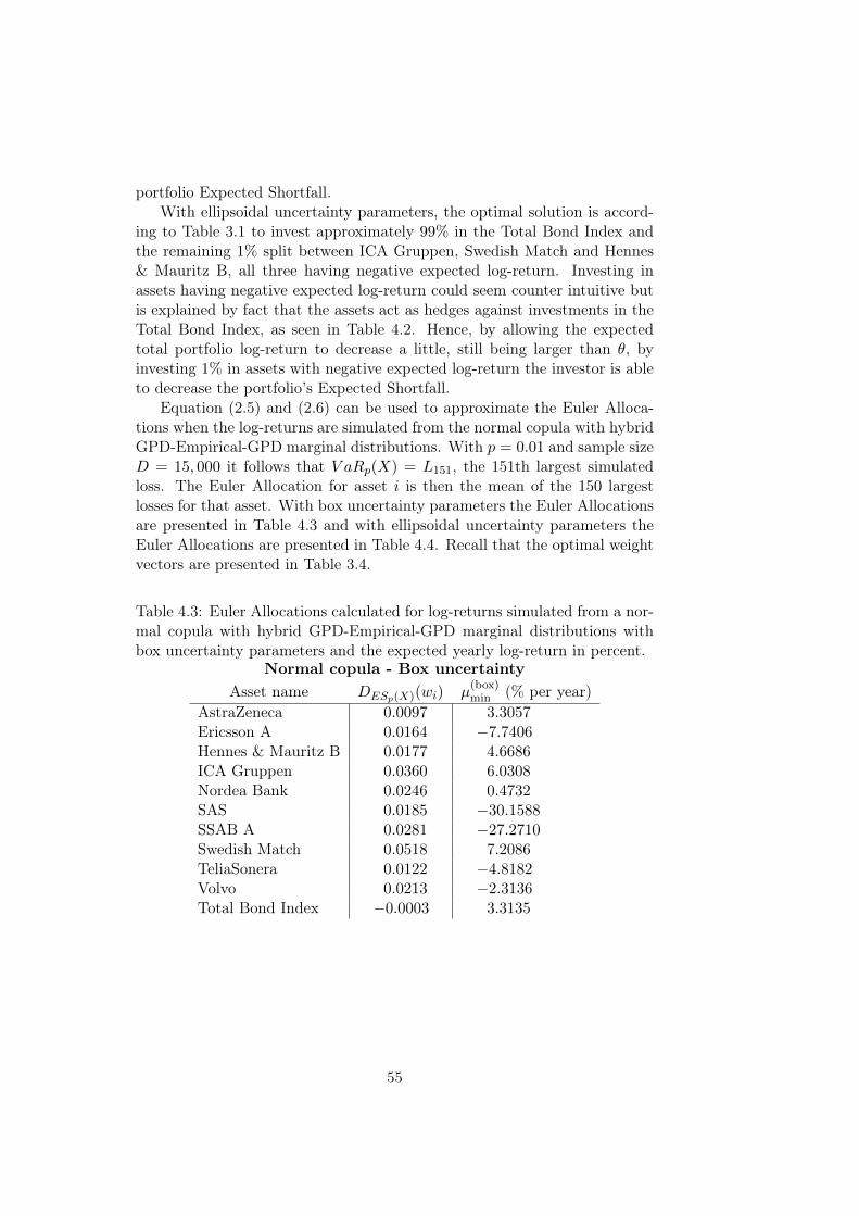
portfolio Expected Shortfall.With ellipsoidal uncertainty parameters, the optimal solution is accord-

ing to Table 3.1 to invest approximately 99% in the Total Bond Index andthe remaining 1% split between ICA Gruppen, Swedish Match and Hennes& Mauritz B, all three having negative expected log-return. Investing inassets having negative expected log-return could seem counter intuitive butis explained by fact that the assets act as hedges against investments in theTotal Bond Index, as seen in Table 4.2. Hence, by allowing the expectedtotal portfolio log-return to decrease a little, still being larger than θ, byinvesting 1% in assets with negative expected log-return the investor is ableto decrease the portfolio’s Expected Shortfall.

Equation (2.5) and (2.6) can be used to approximate the Euler Alloca-tions when the log-returns are simulated from the normal copula with hybridGPD-Empirical-GPD marginal distributions. With p = 0.01 and sample sizeD = 15, 000 it follows that V aRp(X) = L151, the 151th largest simulatedloss. The Euler Allocation for asset i is then the mean of the 150 largestlosses for that asset. With box uncertainty parameters the Euler Allocationsare presented in Table 4.3 and with ellipsoidal uncertainty parameters theEuler Allocations are presented in Table 4.4. Recall that the optimal weightvectors are presented in Table 3.4.

Table 4.3: Euler Allocations calculated for log-returns simulated from a nor-mal copula with hybrid GPD-Empirical-GPD marginal distributions withbox uncertainty parameters and the expected yearly log-return in percent.

Normal copula - Box uncertaintyAsset name DESp(X)(wi) µ

(box)min (% per year)

AstraZeneca 0.0097 3.3057Ericsson A 0.0164 −7.7406Hennes & Mauritz B 0.0177 4.6686ICA Gruppen 0.0360 6.0308Nordea Bank 0.0246 0.4732SAS 0.0185 −30.1588SSAB A 0.0281 −27.2710Swedish Match 0.0518 7.2086TeliaSonera 0.0122 −4.8182Volvo 0.0213 −2.3136Total Bond Index −0.0003 3.3135

55

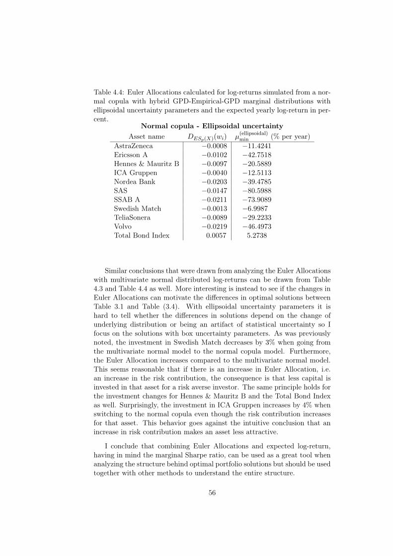
Table 4.4: Euler Allocations calculated for log-returns simulated from a nor-mal copula with hybrid GPD-Empirical-GPD marginal distributions withellipsoidal uncertainty parameters and the expected yearly log-return in per-cent.

Normal copula - Ellipsoidal uncertaintyAsset name DESp(X)(wi) µ

(ellipsoidal)min (% per year)

AstraZeneca −0.0008 −11.4241Ericsson A −0.0102 −42.7518Hennes & Mauritz B −0.0097 −20.5889ICA Gruppen −0.0040 −12.5113Nordea Bank −0.0203 −39.4785SAS −0.0147 −80.5988SSAB A −0.0211 −73.9089Swedish Match −0.0013 −6.9987TeliaSonera −0.0089 −29.2233Volvo −0.0219 −46.4973Total Bond Index 0.0057 5.2738

Similar conclusions that were drawn from analyzing the Euler Allocationswith multivariate normal distributed log-returns can be drawn from Table4.3 and Table 4.4 as well. More interesting is instead to see if the changes inEuler Allocations can motivate the differences in optimal solutions betweenTable 3.1 and Table (3.4). With ellipsoidal uncertainty parameters it ishard to tell whether the differences in solutions depend on the change ofunderlying distribution or being an artifact of statistical uncertainty so Ifocus on the solutions with box uncertainty parameters. As was previouslynoted, the investment in Swedish Match decreases by 3% when going fromthe multivariate normal model to the normal copula model. Furthermore,the Euler Allocation increases compared to the multivariate normal model.This seems reasonable that if there is an increase in Euler Allocation, i.e.an increase in the risk contribution, the consequence is that less capital isinvested in that asset for a risk averse investor. The same principle holds forthe investment changes for Hennes & Mauritz B and the Total Bond Indexas well. Surprisingly, the investment in ICA Gruppen increases by 4% whenswitching to the normal copula even though the risk contribution increasesfor that asset. This behavior goes against the intuitive conclusion that anincrease in risk contribution makes an asset less attractive.

I conclude that combining Euler Allocations and expected log-return,having in mind the marginal Sharpe ratio, can be used as a great tool whenanalyzing the structure behind optimal portfolio solutions but should be usedtogether with other methods to understand the entire structure.

56

4.2 Comments on Worst-Case Scenario Based Ro-bust Optimization

This thesis project has, as commonly done in optimization, interpreted ro-bust optimization as worst-case scenario based optimization, presented inSection 3.1.1. This section discuss the effect of this interpretation on theoptimization problem.

Firstly, worst-case scenario based robust optimization should be seen asa conservative optimization approach. When the worst-case scenarios fromthe uncertainty sets M,S are used in the optimization problem, it meansthat the investor has a more negative view on the market than what theempirically estimated parameters suggests. The investor expects the log-returns of the assets in his portfolio to be worse than it has been historicallyand believes that the assets are more correlated than seen in the covariancematrix. In short, the investor has a conservative view on the market andoptimizes his asset allocations according to his view on the market.

One negative aspect with worst-case scenario based robust optimizationis that the approach is very sensitive to outliers in the historical data. As anexample, with a 95% confidence interval used as uncertainty set, the worst-case scenario is more extreme when outliers are present in the historical datathan what the worst-case scenario would be with no outliers. This results inan even more conservative view on the market for the investor. One approachto solve this problem is to search the data for outliers and remove them priorto constructing the 95% confidence interval.

A positive aspect with the worst-case scenario based robust optimizationapproach is that the solution is quite stable if re-solving the problem period-ically as more historical data is available. This is positive in the sense thatthe investor does not need to re-balance his asset allocations very often andtrading fees can be held low for the investor.

An alternative approach to worst-case scenario based robust optimizationcould be to grid the uncertainty sets and solve the optimization problem foreach combination of realizations in each uncertainty set and then analyze howthe solution changes as function of parameter location within the uncertaintysets. This approach would however be very time consuming and perhapscomputationally impossible to solve with many assets in the portfolio andfine grids of the uncertainty sets.

4.3 More Comments and Further Investigation

The thesis project ends by a few remarks on some alternative approaches thatcould have been used and discuss areas where further investigation could beof interest.

In this thesis project the worst-case box uncertainty log-return µ(box)min

57

is constructed as in (3.2) by subtracting 20% of each element in the vec-tor. The result is then compared to the lower limit of the 95% confidenceinterval to see whether the worst-case scenario is reasonable or not. An al-ternative approach is to define µ(box)

min directly as the lower limit of the 95%confidence interval. With the particular historical data in this thesis projectthis approach resulted in that all elements in µ

(box)min were negative. This

yields a robust optimization problem without solutions since the constraintwTµmin ≥ θ cannot be satisfied with long positions. In light of this, thisalternative approach was not used in the thesis project but could be moreintuitive to use in other applications or with other reference portfolios.

All solutions in this thesis project are based on the same reference portfo-lio with assets listed in Table 1.1. It would however be interesting to analyzehow different reference portfolios consisting of other types of financial as-sets affect the optimal solution. For instance, how is the optimal solutionaffected if the amount of financial assets included in the reference portfolioincreases? It seems reasonable that larger reference portfolios would decreasethe Expected Shortfall since the optimization algorithm has more assets tochoose from. However, as has been seen in all solutions throughout thisthesis project, the optimal solution often turns out to be to investment ina small sub group of the possible assets. Therefore, including more assetsin the reference portfolio does not necessarily decrease the risk and couldat worst result in a less time efficient program that can be crucial for theinvestor. What can be said is that including more assets in the referenceportfolio does at least not increase the financial risk. The perhaps mostinteresting area of further investigation would be to extend the referenceportfolio to include other types of financial assets such as foreign curren-cies or non-linear financial derivatives such as options. This would introducepossibilities of more complex hedging opportunities than possible with linearassets. It is furthermore interesting because non-linear portfolios makes fulluse of the risk measure Expected Shortfall since Markowitz mean-varianceoptimization problem cannot handle non-linear financial assets. In that casethe non-linear assets have to be approximated by linear functions. Thirdlyit would be interesting from a practical point of view to include non-linearassets since it is common that investors have non-linear assets in their port-folios.

In this thesis project, the p-value has been held constant to 1% but canof course be altered as well. Decreasing the p-value should however onlyincrease the Expected Shortfall or the investor must decrease the thresholdfor acceptable expected log-return to keep the risk constant. Hence theinvestor has to find a p-level where he feels confident with both the expectedportfolio log-return and the risk he is exposed to.

Another interesting area of further investigation is to study the effect ofdifferent copulas on the optimal solution. In this thesis project, the normal

58

copula was used together with hybrid GPD-Empirical-GPD marginal dis-tributions but the dependency structure between different log-returns couldjust as well had been modeled by another copula. However, as was men-tioned earlier, according to Skoglund and Nyström the choice of copula hasa second-order effect on the model accuracy when modeling market risk fac-tors. If a Student’s t copula were used instead, the results had probably onlybeen marginally improved.

The last area that I will mention where further investigation could bemade is in the decision of the upper and lower thresholds for the generalizedPareto distributions. In this thesis project the thresholds were chosen as the90% and 10% empirical quantiles respectively but no investigation was madeto establish whether these thresholds were good representatives of where thetails begin. A better and more consistent approach to find the thresholds isto use a parametric estimation method such as the Hill’s tail-index estimator[4]. This could improve the results a bit further but also make the programmore time consuming.

Different approaches taken in a portfolio optimization problem, whetherit is about which problem formulation to use, which models to use or whichparameters to use, is ultimately up to the investor to decide and a trade-off between model accuracy and time efficiency/computational possibilityalways has to be considered.

59

60

Appendix A

Optimization Parameters

When solving the portfolio optimization problem (2.16) the parameters µ andΣ are needed for instance in the process of simulating log-returns. Since theportfolio lives for one day, µ is the expected daily log-return and Σ is the co-variance matrix for daily log-returns. In the thesis project I begin by solvingthe portfolio optimization problem with empirically estimated parametersfrom historical data and then solve the robust portfolio optimization prob-lem (3.1) after manipulating the empirical parameters to obtain two differentkinds of worst-case scenario parameters. The worst-case scenario box uncer-tainty parameters are defined by (3.2) and (3.3) and the worst-case scenarioellipsoidal uncertainty parameters are defined by (3.4) and (3.5). In thisAppendix I clarify the parameters by writing out their explicit numericalvalues.

The numerical values of the empirical parameters estimated for the timeperiod January 2, 2007 until January 22, 2016 from daily log-return data tothe assets in the reference portfolio are

µ = 10−4 [1.6463 −2.5699 2.3250 3.0034 0.2357 −10.0129 −9.0541 3.5899 −1.5997 −0.7681 1.6501

]T

Σ = 10−4

2.2076 0.8564 0.7462 0.5434 0.8873 0.9597 0.9827 0.6127 0.7489 0.8089 −0.02010.8564 6.7548 1.4816 0.8375 2.3592 1.8613 2.5425 0.8313 1.3073 2.5546 −0.06880.7462 1.4816 2.6549 0.8594 1.9553 1.7679 2.1897 0.7987 1.2000 2.0837 −0.06060.5434 0.8375 0.8594 3.2819 1.2290 1.2987 1.4293 0.4836 0.8364 1.3421 −0.04240.8873 2.3592 1.9553 1.2290 4.9191 2.7372 3.5812 1.0444 1.8956 3.3907 −0.10520.9597 1.8613 1.7679 1.2987 2.7372 13.5689 3.0979 0.7071 1.5030 2.9935 −0.08210.9827 2.5425 2.1897 1.4293 3.5812 3.0979 8.3021 1.0916 1.9876 4.4259 −0.12170.6127 0.8313 0.7987 0.4836 1.0444 0.7071 1.0916 2.4675 0.7539 1.0733 −0.02710.7489 1.3073 1.2000 0.8364 1.8956 1.5030 1.9876 0.7539 2.6576 1.9369 −0.05380.8089 2.5546 2.0837 1.3421 3.3907 2.9935 4.4259 1.0733 1.9369 5.8128 −0.1094−0.0201 −0.0688 −0.0606 −0.0424 −0.1052 −0.0821 −0.1217 −0.0271 −0.0538 −0.1094 0.0195

.

The numerical values of the box uncertainty parameters defined by (3.2) and(3.3) are

61

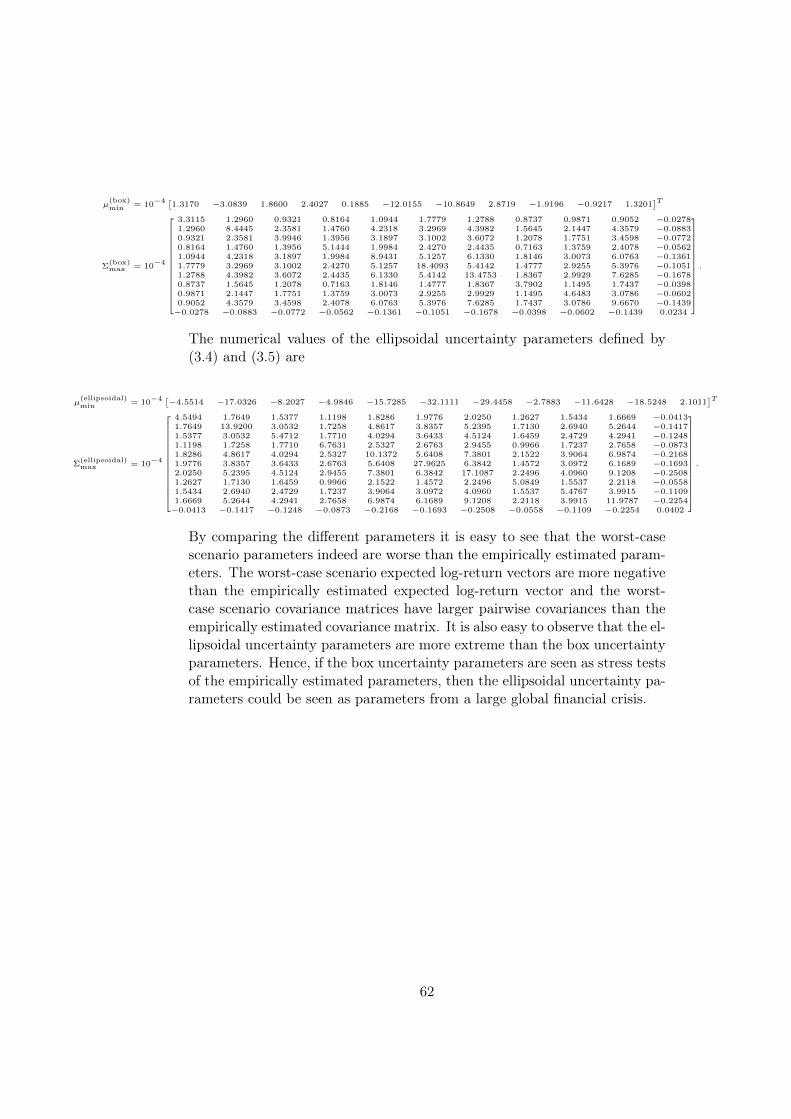
µ(box)min = 10

−4 [1.3170 −3.0839 1.8600 2.4027 0.1885 −12.0155 −10.8649 2.8719 −1.9196 −0.9217 1.3201]T

Σ(box)max = 10

−4

3.3115 1.2960 0.9321 0.8164 1.0944 1.7779 1.2788 0.8737 0.9871 0.9052 −0.02781.2960 8.4445 2.3581 1.4760 4.2318 3.2969 4.3982 1.5645 2.1447 4.3579 −0.08830.9321 2.3581 3.9946 1.3956 3.1897 3.1002 3.6072 1.2078 1.7751 3.4598 −0.07720.8164 1.4760 1.3956 5.1444 1.9984 2.4270 2.4435 0.7163 1.3759 2.4078 −0.05621.0944 4.2318 3.1897 1.9984 8.9431 5.1257 6.1330 1.8146 3.0073 6.0763 −0.13611.7779 3.2969 3.1002 2.4270 5.1257 18.4093 5.4142 1.4777 2.9255 5.3976 −0.10511.2788 4.3982 3.6072 2.4435 6.1330 5.4142 13.4753 1.8367 2.9929 7.6285 −0.16780.8737 1.5645 1.2078 0.7163 1.8146 1.4777 1.8367 3.7902 1.1495 1.7437 −0.03980.9871 2.1447 1.7751 1.3759 3.0073 2.9255 2.9929 1.1495 4.6483 3.0786 −0.06020.9052 4.3579 3.4598 2.4078 6.0763 5.3976 7.6285 1.7437 3.0786 9.6670 −0.1439−0.0278 −0.0883 −0.0772 −0.0562 −0.1361 −0.1051 −0.1678 −0.0398 −0.0602 −0.1439 0.0234

.

The numerical values of the ellipsoidal uncertainty parameters defined by(3.4) and (3.5) are

µ(ellipsoidal)min = 10

−4 [−4.5514 −17.0326 −8.2027 −4.9846 −15.7285 −32.1111 −29.4458 −2.7883 −11.6428 −18.5248 2.1011]T

Σ(ellipsoidal)max = 10

−4

4.5494 1.7649 1.5377 1.1198 1.8286 1.9776 2.0250 1.2627 1.5434 1.6669 −0.04131.7649 13.9200 3.0532 1.7258 4.8617 3.8357 5.2395 1.7130 2.6940 5.2644 −0.14171.5377 3.0532 5.4712 1.7710 4.0294 3.6433 4.5124 1.6459 2.4729 4.2941 −0.12481.1198 1.7258 1.7710 6.7631 2.5327 2.6763 2.9455 0.9966 1.7237 2.7658 −0.08731.8286 4.8617 4.0294 2.5327 10.1372 5.6408 7.3801 2.1522 3.9064 6.9874 −0.21681.9776 3.8357 3.6433 2.6763 5.6408 27.9625 6.3842 1.4572 3.0972 6.1689 −0.16932.0250 5.2395 4.5124 2.9455 7.3801 6.3842 17.1087 2.2496 4.0960 9.1208 −0.25081.2627 1.7130 1.6459 0.9966 2.1522 1.4572 2.2496 5.0849 1.5537 2.2118 −0.05581.5434 2.6940 2.4729 1.7237 3.9064 3.0972 4.0960 1.5537 5.4767 3.9915 −0.11091.6669 5.2644 4.2941 2.7658 6.9874 6.1689 9.1208 2.2118 3.9915 11.9787 −0.2254−0.0413 −0.1417 −0.1248 −0.0873 −0.2168 −0.1693 −0.2508 −0.0558 −0.1109 −0.2254 0.0402

.

By comparing the different parameters it is easy to see that the worst-casescenario parameters indeed are worse than the empirically estimated param-eters. The worst-case scenario expected log-return vectors are more negativethan the empirically estimated expected log-return vector and the worst-case scenario covariance matrices have larger pairwise covariances than theempirically estimated covariance matrix. It is also easy to observe that the el-lipsoidal uncertainty parameters are more extreme than the box uncertaintyparameters. Hence, if the box uncertainty parameters are seen as stress testsof the empirically estimated parameters, then the ellipsoidal uncertainty pa-rameters could be seen as parameters from a large global financial crisis.

62

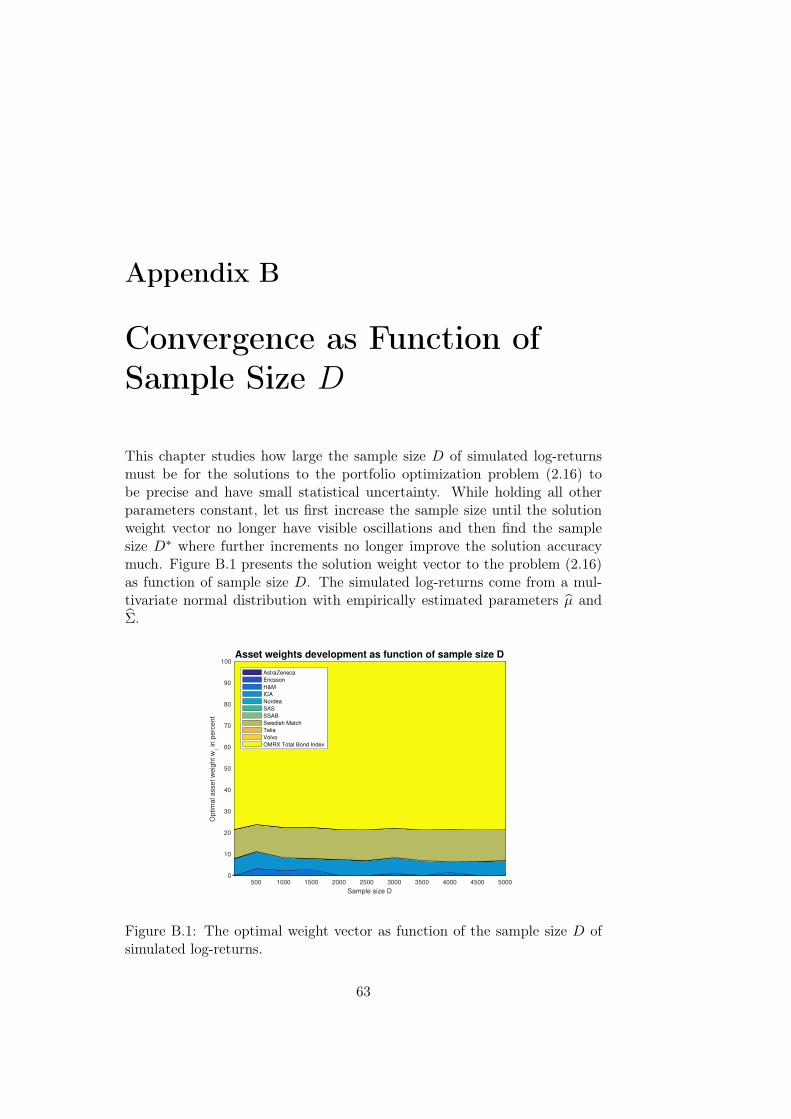
Appendix B

Convergence as Function ofSample Size D

This chapter studies how large the sample size D of simulated log-returnsmust be for the solutions to the portfolio optimization problem (2.16) tobe precise and have small statistical uncertainty. While holding all otherparameters constant, let us first increase the sample size until the solutionweight vector no longer have visible oscillations and then find the samplesize D∗ where further increments no longer improve the solution accuracymuch. Figure B.1 presents the solution weight vector to the problem (2.16)as function of sample size D. The simulated log-returns come from a mul-tivariate normal distribution with empirically estimated parameters µ andΣ.

500 1000 1500 2000 2500 3000 3500 4000 4500 5000

Sample size D

0

10

20

30

40

50

60

70

80

90

100

Optim

al asset w

eig

ht w

i in p

erc

ent

Asset weights development as function of sample size D

AstraZeneca

Ericsson

H&M

ICA

Nordea

SAS

SSAB

Swedish Match

Telia

Volvo

OMRX Total Bond Index

Figure B.1: The optimal weight vector as function of the sample size D ofsimulated log-returns.

63

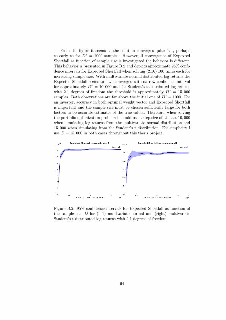
From the figure it seems as the solution converges quite fast, perhapsas early as for D∗ = 1000 samples. However, if convergence of ExpextedShortfall as function of sample size is investigated the behavior is different.This behavior is presented in Figure B.2 and depicts approximate 95% confi-dence intervals for Expected Shortfall when solving (2.16) 100 times each forincreasing sample size. With multivariate normal distributed log-returns theExpected Shortfall seems to have converged with narrow confidence intervalfor approximately D∗ = 10, 000 and for Student’s t distributed log-returnswith 2.1 degrees of freedom the threshold is approximately D∗ = 15, 000samples. Both observations are far above the initial one of D∗ = 1000. Foran investor, accuracy in both optimal weight vector and Expected Shortfallis important and the sample size must be chosen sufficiently large for bothfactors to be accurate estimates of the true values. Therefore, when solvingthe portfolio optimization problem I should use a step size of at least 10, 000when simulating log-returns from the multivariate normal distribution and15, 000 when simulating from the Student’s t distribution. For simplicity Iuse D = 15, 000 in both cases throughout this thesis project.

Figure B.2: 95% confidence intervals for Expected Shortfall as function ofthe sample size D for (left) multivariate normal and (right) multivariateStudent’s t distributed log-returns with 2.1 degrees of freedom.

64

Appendix C

Reference Solutions

This Appendix presents reference solutions to the robust portfolio opti-mization problem (3.1) when instead Markowitz mean-variance optimizationproblem (1.3) is solved. By doing this, statistical uncertainty is avoided. Thetwo optimization problems are connected through the risk aversion coefficientc which for elliptically distributed log-returns is calculated as (2.11). The ref-erence portfolio Expected Shortfall in the last row of each table is calculatedusing (2.17) and (2.18).

C.1 Normal Distributed Log-returns

Under the assumption of multivariate normal distributed log-returns, therisk aversion coefficient c in Markowitz mean-variance optimization problemis already calculated in (2.12) to be c = 5.33. With the same worst-casescenario parameters µmin and Σmax used to obtain the two solutions in Ta-ble 3.1, the corresponding reference solutions to Markowitz mean-varianceproblem (1.3) are presented in Table C.1.

65

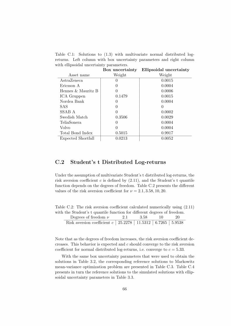
Table C.1: Solutions to (1.3) with multivariate normal distributed log-returns. Left column with box uncertainty parameters and right columnwith ellipsoidal uncertainty parameters.

Box uncertainty Ellipsoidal uncertaintyAsset name Weight Weight

AstraZeneca 0 0.0015Ericsson A 0 0.0004Hennes & Mauritz B 0 0.0006ICA Gruppen 0.1479 0.0015Nordea Bank 0 0.0004SAS 0 0SSAB A 0 0.0002Swedish Match 0.3506 0.0029TeliaSonera 0 0.0004Volvo 0 0.0004Total Bond Index 0.5015 0.9917

Expected Shortfall 0.0213 0.0052

C.2 Student’s t Distributed Log-returns

Under the assumption of multivariate Student’s t distributed log-returns, therisk aversion coefficient c is defined by (2.11), and the Student’s t quantilefunction depends on the degrees of freedom. Table C.2 presents the differentvalues of the risk aversion coefficient for ν = 2.1, 3.58, 10, 20.

Table C.2: The risk aversion coefficient calculated numerically using (2.11)with the Student’s t quantile function for different degrees of freedom.

Degrees of freedom ν 2.1 3.58 10 20

Risk aversion coefficient c 25.2278 11.5312 6.7265 5.9538

Note that as the degrees of freedom increases, the risk aversion coefficient de-creases. This behavior is expected and c should converge to the risk aversioncoefficient for normal distributed log-returns, i.e. converge to c = 5.33.

With the same box uncertainty parameters that were used to obtain thesolutions in Table 3.2, the corresponding reference solutions to Markowitzmean-variance optimization problem are presented in Table C.3. Table C.4presents in turn the reference solutions to the simulated solutions with ellip-soidal uncertainty parameters in Table 3.3.

66

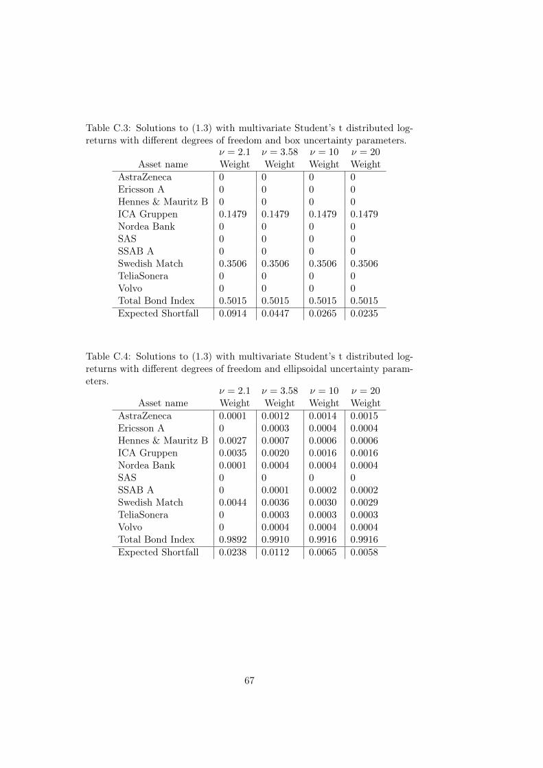
Table C.3: Solutions to (1.3) with multivariate Student’s t distributed log-returns with different degrees of freedom and box uncertainty parameters.

ν = 2.1 ν = 3.58 ν = 10 ν = 20Asset name Weight Weight Weight Weight

AstraZeneca 0 0 0 0Ericsson A 0 0 0 0Hennes & Mauritz B 0 0 0 0ICA Gruppen 0.1479 0.1479 0.1479 0.1479Nordea Bank 0 0 0 0SAS 0 0 0 0SSAB A 0 0 0 0Swedish Match 0.3506 0.3506 0.3506 0.3506TeliaSonera 0 0 0 0Volvo 0 0 0 0Total Bond Index 0.5015 0.5015 0.5015 0.5015

Expected Shortfall 0.0914 0.0447 0.0265 0.0235

Table C.4: Solutions to (1.3) with multivariate Student’s t distributed log-returns with different degrees of freedom and ellipsoidal uncertainty param-eters.

ν = 2.1 ν = 3.58 ν = 10 ν = 20Asset name Weight Weight Weight Weight

AstraZeneca 0.0001 0.0012 0.0014 0.0015Ericsson A 0 0.0003 0.0004 0.0004Hennes & Mauritz B 0.0027 0.0007 0.0006 0.0006ICA Gruppen 0.0035 0.0020 0.0016 0.0016Nordea Bank 0.0001 0.0004 0.0004 0.0004SAS 0 0 0 0SSAB A 0 0.0001 0.0002 0.0002Swedish Match 0.0044 0.0036 0.0030 0.0029TeliaSonera 0 0.0003 0.0003 0.0003Volvo 0 0.0004 0.0004 0.0004Total Bond Index 0.9892 0.9910 0.9916 0.9916

Expected Shortfall 0.0238 0.0112 0.0065 0.0058

67

68

Appendix D

GARCH and GPD Parameters

The generalized Pareto distribution Gγ,β(x) is given by

Gγ,β(x) = 1−(

1 +γx

β

)− 1γ

, x ≥ 0

for some shape parameter γ > 0 and scale parameter β > 0 and

Gγ,β(x) = 1− e−xβ , x ≥ 0

if γ = 0.

Modeling excesses in the tail of a distribution over a suitably high thresh-old u with a generalized Pareto distribution is possible if the underlying datais independent and identically distributed. The log-returns in the referenceportfolio can only be assumed to be weakly dependent and close to inde-pendent and identically distributed and typically suffers from the stylizedfacts presented in Section 3.1.3.3. To obtain independent and identically dis-tributed data the historical log-returns to each asset in the reference portfolioare filtered with fitted GARCH(1,1) models, also defined in Section 3.1.3.3.The GARCH(1,1) parameters were numerically estimated with the Maxi-mum Likelihood method using the function estimate in Matlab and arepresented in Table D.1 together with other statistical quantities of interest.

69

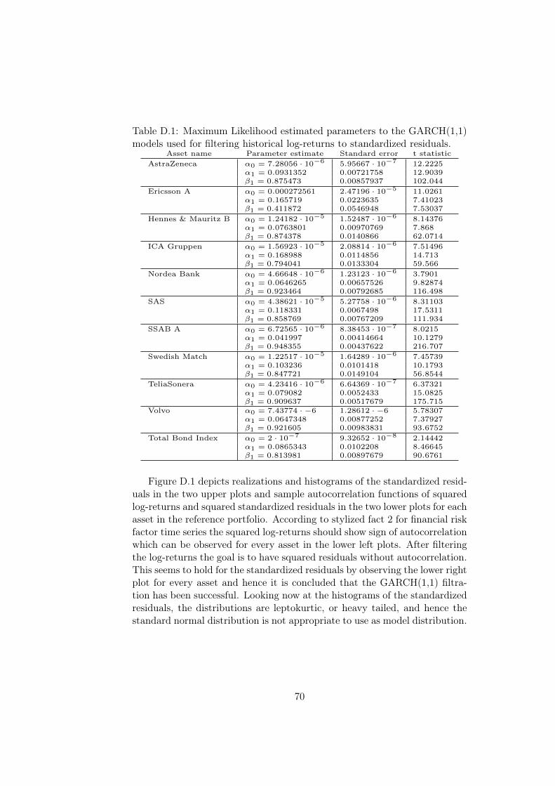
Table D.1: Maximum Likelihood estimated parameters to the GARCH(1,1)models used for filtering historical log-returns to standardized residuals.

Asset name Parameter estimate Standard error t statisticAstraZeneca α0 = 7.28056 · 10−6 5.95667 · 10−7 12.2225

α1 = 0.0931352 0.00721758 12.9039β1 = 0.875473 0.00857937 102.044

Ericsson A α0 = 0.000272561 2.47196 · 10−5 11.0261α1 = 0.165719 0.0223635 7.41023β1 = 0.411872 0.0546948 7.53037

Hennes & Mauritz B α0 = 1.24182 · 10−5 1.52487 · 10−6 8.14376α1 = 0.0763801 0.00970769 7.868β1 = 0.874378 0.0140866 62.0714

ICA Gruppen α0 = 1.56923 · 10−5 2.08814 · 10−6 7.51496α1 = 0.168988 0.0114856 14.713β1 = 0.794041 0.0133304 59.566

Nordea Bank α0 = 4.66648 · 10−6 1.23123 · 10−6 3.7901α1 = 0.0646265 0.00657526 9.82874β1 = 0.923464 0.00792685 116.498

SAS α0 = 4.38621 · 10−5 5.27758 · 10−6 8.31103α1 = 0.118331 0.0067498 17.5311β1 = 0.858769 0.00767209 111.934

SSAB A α0 = 6.72565 · 10−6 8.38453 · 10−7 8.0215α1 = 0.041997 0.00414664 10.1279β1 = 0.948355 0.00437622 216.707

Swedish Match α0 = 1.22517 · 10−5 1.64289 · 10−6 7.45739α1 = 0.103236 0.0101418 10.1793β1 = 0.847721 0.0149104 56.8544

TeliaSonera α0 = 4.23416 · 10−6 6.64369 · 10−7 6.37321α1 = 0.079082 0.0052433 15.0825β1 = 0.909637 0.00517679 175.715

Volvo α0 = 7.43774 · −6 1.28612 · −6 5.78307α1 = 0.0647348 0.00877252 7.37927β1 = 0.921605 0.00983831 93.6752

Total Bond Index α0 = 2 · 10−7 9.32652 · 10−8 2.14442α1 = 0.0865343 0.0102208 8.46645β1 = 0.813981 0.00897679 90.6761

Figure D.1 depicts realizations and histograms of the standardized resid-uals in the two upper plots and sample autocorrelation functions of squaredlog-returns and squared standardized residuals in the two lower plots for eachasset in the reference portfolio. According to stylized fact 2 for financial riskfactor time series the squared log-returns should show sign of autocorrelationwhich can be observed for every asset in the lower left plots. After filteringthe log-returns the goal is to have squared residuals without autocorrelation.This seems to hold for the standardized residuals by observing the lower rightplot for every asset and hence it is concluded that the GARCH(1,1) filtra-tion has been successful. Looking now at the histograms of the standardizedresiduals, the distributions are leptokurtic, or heavy tailed, and hence thestandard normal distribution is not appropriate to use as model distribution.

70

FigureD.1:Eachsubfig

ureconsists

ofrealizations

andhistog

ramsof

thestan

dardized

residu

alsan

dsampleau

tocorrelation

function

sof

squa

redlog-returnsan

dsqua

redstan

dardized

residu

als.

71

The same conclusion can be drawn by observing Figure D.2 which showsQuantile-Quantile plots for the empirical residual quantile function plottedagainst the standard normal quantile function. A good fit should producea straight line and a reverted S-shaped curve indicates that the tails areheavier than for the standard normal distribution. As can be seen, revertedS-shapes appear in every plot indicating that the standardized residuals havedistributions with fatter tails than the standard normal distribution. Noticealso that the S-shapes are asymmetric, meaning that the two tails of theresidual distribution are of different size and length. Therefore, an ellipticaldistribution with fat tails, for instance the Student’s t distribution, would notcapture the entire empirical residual distribution since elliptical distributionsare symmetric. Thus generalized Pareto distributions are appropriate tomodel the tails of the residual distributions since this can give an asymmetricdistribution.

72

-4-3

-2-1

01

23

4

Sta

ndard

Norm

al Q

uantile

s

-8-6-4-202468

Quantiles of Input Sample

QQ

Plo

t o

f S

tan

dard

ized

Resid

uals

to

Astr

aZ

en

eca v

ers

us S

tan

dard

No

rmal

-4-3

-2-1

01

23

4

Sta

ndard

Norm

al Q

uantile

s

-15

-10-505

10

15

20

25

Quantiles of Input Sample

QQ

Plo

t o

f S

tan

dard

ized

Resid

uals

to

Eri

csso

n A

vers

us S

tan

dard

No

rmal

-4-3

-2-1

01

23

4

Sta

ndard

Norm

al Q

uantile

s

-8-6-4-20246

Quantiles of Input Sample

QQ

Plo

t o

f S

tan

dard

ized

Resid

uals

to

Hen

nes &

Mau

ritz

B v

ers

us S

tan

dard

No

rmal

-4-3

-2-1

01

23

4

Sta

ndard

Norm

al Q

uantile

s

-6-4-20246

Quantiles of Input Sample

QQ

Plo

t o

f S

tan

dard

ized

Resid

uals

to

IC

A G

rup

pen

vers

us S

tan

dard

No

rmal

-4-3

-2-1

01

23

4

Sta

ndard

Norm

al Q

uantile

s

-4-3-2-10123456

Quantiles of Input Sample

QQ

Plo

t o

f S

tan

dard

ized

Resid

uals

to

No

rdea B

an

k v

ers

us S

tan

dard

No

rmal

-4-3

-2-1

01

23

4

Sta

ndard

Norm

al Q

uantile

s

-8-6-4-202468

Quantiles of Input Sample

QQ

Plo

t o

f S

tan

dard

ized

Resid

uals

to

SA

S v

ers

us S

tan

dard

No

rmal

-4-3

-2-1

01

23

4

Sta

ndard

Norm

al Q

uantile

s

-6-4-202468

Quantiles of Input Sample

QQ

Plo

t o

f S

tan

dard

ized

Resid

uals

to

SS

AB

A v

ers

us S

tan

dard

No

rmal

-4-3

-2-1

01

23

4

Sta

ndard

Norm

al Q

uantile

s

-6-4-20246

Quantiles of Input Sample

QQ

Plo

t o

f S

tan

dard

ized

Resid

uals

to

Sw

ed

ish

Matc

h v

ers

us S

tan

dard

No

rmal

-4-3

-2-1

01

23

4

Sta

ndard

Norm

al Q

uantile

s

-8-6-4-20246

Quantiles of Input Sample

QQ

Plo

t o

f S

tan

dard

ized

Resid

uals

to

TeliaS

on

era

vers

us S

tan

dard

No

rmal

-4-3

-2-1

01

23

4

Sta

ndard

Norm

al Q

uantile

s

-4-202468

Quantiles of Input Sample

QQ

Plo

t o

f S

tan

dard

ized

Resid

uals

to

Vo

lvo

vers

us S

tan

dard

No

rmal

-4-3

-2-1

01

23

4

Sta

ndard

Norm

al Q

uantile

s

-6-4-202468

Quantiles of Input Sample

QQ

Plo

t o

f S

tan

dard

ized

Resid

uals

to

OM

RX

To

tal B

on

d In

dex v

ers

us S

tan

dard

No

rmal

FigureD.2:Eachsubfig

ureconsists

ofQua

ntile

-Qua

ntile

plotsof

theem

piricalq

uantile

func

tion

forthestan

dardized

residu

als

versus

thestan

dard

norm

alqu

antile

function

.

73

Table D.2 presents Maximum Likelihood estimated parameters to themodeled generalized Pareto distributions with tail thresholds chosen as uh =F−1n (0.90) and ul = F−1

n (0.10) respectively for each asset in the referenceportfolio.

Table D.2: Maximum Likelihood estimated generalized Pareto distributionparameters to standardized residuals calculated for each asset in the referenceportfolio. The thresholds are chosen as uh = F−1

n (0.90) and ul = F−1n (0.10).

Asset name Threshold γ β

AstraZeneca ul = −1.0957 0.1348 0.5897

uh = 1.0984 −0.0127 0.7010

Ericsson A ul = −0.9369 0.1829 0.5844

uh = 0.9762 0.2569 0.4286

Hennes & Mauritz B ul = −1.1497 0.1112 0.5477

uh = 1.1377 0.0701 0.6366

ICA Gruppen ul = −1.1299 −0.0201 0.6120

uh = 1.2474 0.0527 0.6210

Nordea Bank ul = −1.1740 −0.0745 0.5647

uh = 1.2112 0.0104 0.6627

SAS ul = −1.0576 0.1897 0.5085

uh = 1.1622 0.0712 0.6935

SSAB A ul = −1.1388 0.0557 0.5270

uh = 1.2375 0.1244 0.5508

Swedish Match ul = −1.1020 0.1509 0.5094

uh = 1.1974 −0.0139 0.6881

TeliaSonera ul = −1.0573 0.2619 0.4897

uh = 1.1462 0.0709 0.6137

Volvo ul = −1.1655 −0.0123 0.5449

uh = 1.2166 0.0637 0.5970

Total Bond Index ul = −1.2251 0.0695 0.5012

uh = 1.1286 0.2358 0.4493

The thresholds ul and uh and parameters γ and β are used in Section3.1.3.4 when solving the robust optimization problem (3.1). They are usedin Algorithm 1 step 3 when calculating F−1

i being the inverse of the hybridGPD-Empirical-GPD distribution function (3.7).

Figure D.3 displays the generalized Pareto distributions with parametersin Table D.2 together with the empirical cumulative distribution for thestandardized residuals. The estimated tail distributions are found to fit theempirical residual data well in the tails and the hybrid GPD-Empirical-GPDdistributions will reflect the entire residual distribution much more accuratethan the standard normal or Student’s t distribution.

74

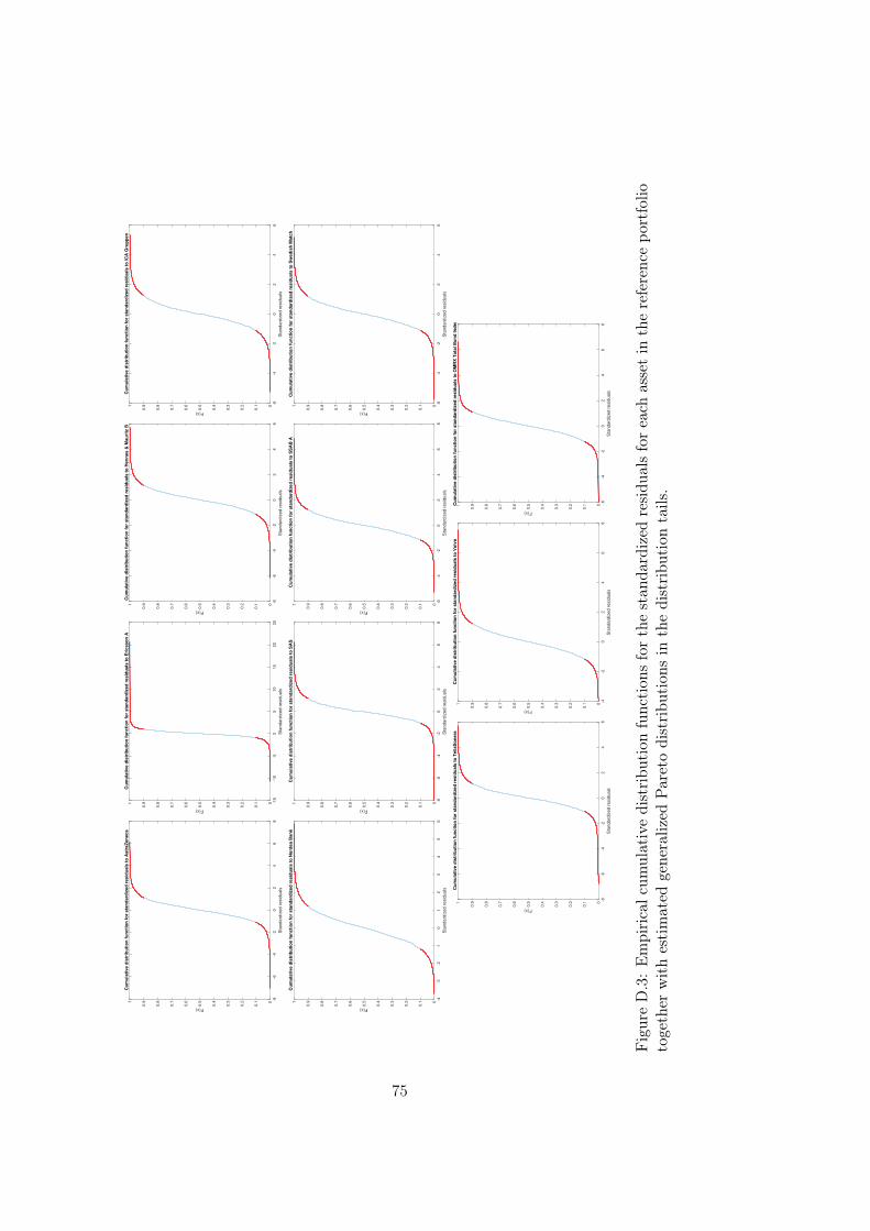
-8-6

-4-2

02

46

8

Sta

nd

ard

ize

d r

esid

ua

ls

0

0.1

0.2

0.3

0.4

0.5

0.6

0.7

0.8

0.91

F(x)

Cu

mu

lati

ve

dis

trib

uti

on

fu

nc

tio

n f

or s

tan

da

rd

ize

d r

es

idu

als

to

As

tra

Ze

ne

ca

-15

-10

-50

510

15

20

25

Sta

nd

ard

ize

d r

esid

ua

ls

0

0.1

0.2

0.3

0.4

0.5

0.6

0.7

0.8

0.91

F(x)

Cu

mu

lati

ve

dis

trib

uti

on

fu

nc

tio

n f

or s

tan

da

rd

ize

d r

es

idu

als

to

Eric

ss

on

A

-8-6

-4-2

02

46

Sta

nd

ard

ize

d r

esid

ua

ls

0

0.1

0.2

0.3

0.4

0.5

0.6

0.7

0.8

0.91

F(x)

Cu

mu

lati

ve

dis

trib

uti

on

fu

nc

tio

n f

or s

tan

da

rd

ize

d r

es

idu

als

to

He

nn

es

& M

au

rit

z B

-6-4

-20

24

6

Sta

nd

ard

ize

d r

esid

ua

ls

0

0.1

0.2

0.3

0.4

0.5

0.6

0.7

0.8

0.91

F(x)

Cu

mu

lati

ve

dis

trib

uti

on

fu

nc

tio

n f

or

sta

nd

ard

ize

d r

es

idu

als

to

IC

A G

rup

pe

n

-4-3

-2-1

01

23

45

6

Sta

nd

ard

ize

d r

esid

ua

ls

0

0.1

0.2

0.3

0.4

0.5

0.6

0.7

0.8

0.91

F(x)

Cu

mu

lati

ve

dis

trib

uti

on

fu

nc

tio

n f

or s

tan

da

rd

ize

d r

es

idu

als

to

No

rd

ea

Ba

nk

-8-6

-4-2

02

46

8

Sta

nd

ard

ize

d r

esid

ua

ls

0

0.1

0.2

0.3

0.4

0.5

0.6

0.7

0.8

0.91

F(x)

Cu

mu

lati

ve

dis

trib

uti

on

fu

nc

tio

n f

or s

tan

da

rd

ize

d r

es

idu

als

to

SA

S

-6-4

-20

24

68

Sta

nd

ard

ize

d r

esid

ua

ls

0

0.1

0.2

0.3

0.4

0.5

0.6

0.7

0.8

0.91

F(x)

Cu

mu

lati

ve

dis

trib

uti

on

fu

nc

tio

n f

or s

tan

da

rd

ize

d r

es

idu

als

to

SS

AB

A

-6-4

-20

24

6

Sta

nd

ard

ize

d r

esid

ua

ls

0

0.1

0.2

0.3

0.4

0.5

0.6

0.7

0.8

0.91

F(x)

Cu

mu

lati

ve

dis

trib

uti

on

fu

nc

tio

n f

or s

tan

da

rd

ize

d r

es

idu

als

to

Sw

ed

ish

Ma

tch

-8-6

-4-2

02

46

Sta

nd

ard

ize

d r

esid

ua

ls

0

0.1

0.2

0.3

0.4

0.5

0.6

0.7

0.8

0.91

F(x)

Cu

mu

lati

ve

dis

trib

uti

on

fu

nc

tio

n f

or s

tan

da

rd

ize

d r

es

idu

als

to

Te

lia

So

ne

ra

-4-2

02

46

8

Sta

nd

ard

ize

d r

esid

ua

ls

0

0.1

0.2

0.3

0.4

0.5

0.6

0.7

0.8

0.91

F(x)

Cu

mu

lati

ve

dis

trib

uti

on

fu

nc

tio

n f

or s

tan

da

rd

ize

d r

es

idu

als

to

Vo

lvo

-6-4

-20

24

68

Sta

nd

ard

ize

d r

esid

ua

ls

0

0.1

0.2

0.3

0.4

0.5

0.6

0.7

0.8

0.91

F(x)

Cu

mu

lati

ve

dis

trib

uti

on

fu

nc

tio

n f

or s

tan

da

rd

ize

d r

es

idu

als

to

OM

RX

To

tal

Bo

nd

In

de

x

FigureD.3:Empiricalc

umulativedistribu

tion

function

sforthestan

dardized

residu

alsforeach

assetin

thereferenc

epo

rtfolio

together

withestimated

generaliz

edParetodistribu

tion

sin

thedistribu

tion

tails.

75

76

Bibliography

[1] Peter J Brockwell and Richard A Davis. Introduction to time series andforecasting. Springer Science & Business Media, 2006.

[2] Umberto Cherubini, Elisa Luciano, and Walter Vecchiato. Copula meth-ods in finance. John Wiley & Sons, 2004.

[3] Igor Griva, Stephen G Nash, and Ariela Sofer. Linear and nonlinearoptimization. Siam, 2009.

[4] Bruce M. Hill. A simple general approach to inference about the tailof a distribution. The annals of statistics, 3(5):1163–1174. Institute ofMathematical Statistics, 1975.

[5] Henrik Hult, Filip Lindskog, Ola Hammarlid, and Carl Johan Rehn.Risk and portfolio analysis: Principles and methods. Springer Science& Business Media, 2012.

[6] Gareth James, Daniela Witten, Trevor Hastie, and Robert Tibshirani.An introduction to statistical learning, volume 112. Springer, 2013.

[7] Marcus Josefsson. A copula evt-based approach for measuring tail re-lated risk: Applied on the Swedish market. Master’s thesis, Royal Insti-tute of Technology, 2004.

[8] Patrick Kingsley. Financial crisis: timeline. The Guardian, 7 August2012.

[9] Damon Levine. Modeling tail behavior with extreme value theory. RiskManagement, (17):14–18, September 2009.

[10] Filip Lindskog, Alexander Mcneil, and Uwe Schmock. Kendall’s tau forelliptical distributions. Springer, 2003.

[11] Miguel Sousa Lobo and Stephen Boyd. The worst-case risk of a portfo-lio. Unpublished manuscript. Available from http: // faculty. fuqua.duke. edu/ %7Emlobo/ bio/ researchfiles/ rsk-bnd. pdf , 2000.

77

[12] Harry Markowitz. Portfolio selection. The Journal of Finance, 7(1):77–91. American Finance Association, Wiley, 1952.

[13] Kaj Nyström and Jimmy Skoglund. Efficient filtering of financial timeseries and extreme value theory. Journal of Risk, 7(2):63–84, 2005.

[14] Riccardo Rebonato and Peter Jäckel. The most general methodology tocreate a valid correlation matrix for risk management and option pricingpurposes. Available at SSRN 1969689, 1999.

[15] R Tyrrell Rockafellar and Stanislav Uryasev. Optimization of condi-tional value-at-risk. Journal of risk, 2:21–42, 2000.

[16] Bernd Scherer. Portfolio Construction and Risk Budgeting, 5 ed. RiskBooks, London, Great Britain, 2015.

[17] William F Sharpe. The sharpe ratio. The journal of portfolio manage-ment, 21(1):49–58. Institutional Investor Journals, 1994.

[18] Jimmy Skoglund and Wei Chen. Risk contributions, information andreverse stress testing. The Journal of Risk Model Validation, 3(2):61–77.Incisive Media Plc, 2009.

[19] Jimmy Skoglund and Wei Chen. Financial Risk Management - Applica-tions in Market, Credit, Asset and Liability Management and FirmwideRisk. Wiley Finance Series, 2015.

[20] Dirk Tasche. Risk contributions and performance measurement. Reportof the Lehrstuhl für mathematische Statistik, TU München. Citeseer,1999.

[21] Dirk Tasche. Conditional expectation as quantile derivative. arXivpreprint math/0104190, 2001.

[22] Reha H Tütüncü and M Koenig. Robust asset allocation. Annals ofOperations Research, 132(1-4):157–187. Springer, 2004.

[23] Kai Ye, Panos Parpas, and Berç Rustem. Robust portfolio optimiza-tion: a conic programming approach. Computational Optimization andApplications, 52(2):463–481. Springer, 2012.

78