robust planning and execution - etda
TRANSCRIPT

The Pennsylvania State University
The Graduate School
The Harold and Inge Marcus Department of Industrial and Manufacturing Engineering
ROBUST PLANNING AND EXECUTION
A Dissertation in
Industrial Engineering
by
Yooneun Lee
© 2017 Yooneun Lee
Submitted in Partial Fulfillment
of the Requirements
for the Degree of
Doctor of Philosophy
May 2017

ii
The dissertation of Yooneun Lee was reviewed and approved* by the following:
Vittaldas V. Prabhu
Professor of Industrial and Manufacturing Engineering
Dissertation Advisor
Chair of Committee
Uday V. Shanbhag
Professor of Industrial and Manufacturing Engineering
Tao Yao
Associate Professor of Industrial and Manufacturing Engineering
Mort D. Webster
Associate Professor of Energy Engineering
Janis Terpenny
Professor of Industrial and Manufacturing Engineering
Peter and Angela Dal Pezzo Department Head/Professor
*Signatures are on file in the Graduate School

iii
ABSTRACT
Uncertainties in a system environment have an adverse impact on the system. The system will yield
suboptimal results, inhibit real-time adjustments, and may incur excessive costs for redesign. One of the
most common managerial strategies to deal with such uncertainties is to incorporate redundant buffers in
planning to absorb changes in system parameters, but more often than not, this strategy leads to waste of
resources. Robust optimization is a method to deal with such parameter uncertainties. It postulates the worst
case scenario and obtains a solution that provides a protection against the uncertainty. Plans designed for
the worst tend to be overengineered; in many cases, when uncertain parameters are revealed, the degree of
uncertainty turns out to be no greater than estimated. This effect may lead to underutilization of resources
and inflated costs.
Here we present methods for robust planning and execution in various applications. We first consider the
problem of scheduling operating rooms for surgeries. In order to avoid allocation of excessive resources
and limit the conservativeness of the robust solution, we apply a cardinality-based robust approach. This
enables us to control the level of protection in accordance with the solution quality. Experimental results
based on real hospital data indicate that our method outperforms the practical gap-based approach in terms
of both overtime and underutilization.
We next suggest a robust productivity index (RPI) to measure organizational performance in a dynamic
environment. Compared to the traditional productivity index, it can be used for monitoring time-dependent
performance and detecting exceptions. Efficiencies of service providers are evaluated based on panel data
on youth outcomes from a selected community prevention program. The results suggest that our approach
not only recognizes patterns of productivity progression, but also enables classification of the innovators.
Lastly, we study the real-time adaptive control and monitoring algorithm of an adaptive Work in Process
(WIP) method. The simulation results suggest benefits of the algorithm as a decision support tool for

iv
managing work-in-process and throughput level. Convergence and robustness of the algorithm are also
investigated.
For each of these applications, the proposed method is validated and supported in an appropriate manner
with detailed discussion of accuracy.

v
TABLE OF CONTENTS
LIST OF TABLES ..................................................................................................................................... viii
LIST OF FIGURES ..................................................................................................................................... ix
1 INTRODUCTION ................................................................................................................................ 1
2 ROBUST SUERGERY PLANNING AND EXECUTION .................................................................. 4
2.1 Introduction ................................................................................................................................... 4
2.2 Literature Review .......................................................................................................................... 6
2.3 Model Formulation ....................................................................................................................... 8
2.3.1 Baseline surgery planning model .......................................................................................... 9
2.3.2 Robust surgery planning ..................................................................................................... 11
2.3.3 Solution methods................................................................................................................. 13
2.4 Experimental Results .................................................................................................................. 15
2.4.1 Quality of the robust operational plan ................................................................................. 15
2.4.2 Sensitivity analysis of robust parameters ............................................................................ 18
2.5 Small Hospital Case study .......................................................................................................... 20
2.5.1 Data description .................................................................................................................. 20
2.5.2 Comparison of key performance indicators ........................................................................ 21
2.5.3 Schedule disruptions in execution ....................................................................................... 25
2.6 Large Hospital Case Study .......................................................................................................... 30
2.6.1 Data set and experiment ...................................................................................................... 30
2.7 Implication and Applicability of Results to Other Hospitals ...................................................... 34

vi
2.8 Conclusion .................................................................................................................................. 35
3 EVALUATAION AND MONITORING COMMUNITY YOUTH PREVENTION PROGRAMS
USING ROBUST PRODUCTIVITY INDEX ............................................................................................ 37
3.1 Introduction ................................................................................................................................. 37
3.2 Background ................................................................................................................................. 38
3.2.1 Planning prevention services .............................................................................................. 38
3.2.2 Performance evaluation using DEA .................................................................................... 40
3.2.3 Malmquist Productivity Index ............................................................................................ 42
3.3 Monitoring Performance ............................................................................................................. 47
3.3.1 Robust distance functions ................................................................................................... 47
3.3.2 Constructing productivity bounds ....................................................................................... 53
3.4 An Application of Community Youth Prevention Programs ...................................................... 55
3.4.1 Data and variables ............................................................................................................... 56
3.4.2 Results ................................................................................................................................. 62
3.5 Implementation and Integration of Monitoring Engine .............................................................. 74
3.6 Conclusions ................................................................................................................................. 75
4 REAL-TIME SUPPLY CHAIN CONTROL USING ADAPTIVE WIP ALGORITHM .................. 77
4.1 Introduction ................................................................................................................................. 77
4.2 Literature Review of Card Controlling System .......................................................................... 78
4.2.1 Kanban and CONWIP system ............................................................................................. 78
4.2.2 Self-regulated WIP (SWIP) ................................................................................................ 80

vii
4.3 Adaptive WIP (AWIP) Design ................................................................................................... 83
4.3.1 AWIP integral controller ..................................................................................................... 83
4.3.2 AWIP algorithm .................................................................................................................. 86
4.4 Performance of AWIP Algorithm ............................................................................................... 88
4.4.1 Solution quality ................................................................................................................... 88
4.4.2 Fidelity of the AWIP algorithm .......................................................................................... 93
4.4.3 The AWIP algorithm versus the mathematical model ........................................................ 95
4.5 Concluding Remarks ................................................................................................................. 100
5 CONCLUSION AND FUTURE RESEARCH ................................................................................. 101
5.1 Conclusion ................................................................................................................................ 101
5.2 Future Research ........................................................................................................................ 102
REFERENCES ......................................................................................................................................... 103

viii
LIST OF TABLES
Table 2.1 Experimental Design ................................................................................................................... 16
Table 2.2 Instances ...................................................................................................................................... 16
Table 2.3 Summary of results for 10-surgery samples for robust method .................................................. 17
Table 2.4 Summary of results for 15-surgery samples for robust method .................................................. 18
Table 2.5 Statistics on surgery duration for both planned and exceedance cases ....................................... 21
Table 2.6 Underutilization in robust models and fixed gap model ............................................................. 24
Table 2.7 Summary of comparison between FG and RO models ............................................................... 25
Table 2.8 Empirical distribution of surgery duration and its interval ......................................................... 27
Table 2.9 Probability of disruption and changes in the total cost ............................................................... 29
Table 2.10 Cost increase of gap planning model ........................................................................................ 35
Table 3.1 Variables ..................................................................................................................................... 57
Table 3.2 Input and output variables by quarter ......................................................................................... 59
Table 3.3 Comparative efficiency by fiscal year ........................................................................................ 63
Table 3.4 Average annual productivity growth of the youth prevention program over FY 2010-FY 2015 65
Table 3.5 Average quarterly changes by site .............................................................................................. 66
Table 3.6 Sites shifting the technology frontier .......................................................................................... 67
Table 3.7 Detailed components information associated with upper and lower limits ................................ 72
Table 4.1 Notations ..................................................................................................................................... 84
Table 4.2 AWIP Algorithm ......................................................................................................................... 88
Table 4.3 Performance measures and numerical results ............................................................................. 90
Table 4.4 Relative results of optimization model compared to the AWIP results ...................................... 98

ix
LIST OF FIGURES
Figure 1.1 Hierarchical illustrations of planning layers in the supply chain domain .................................... 1
Figure 2.1 Linkage between planning and execution phases in exception analytics for surgery system ..... 5
Figure 2.2 Daily surgery schedule with three shared ORs ............................................................................ 9
Figure 2.3 Sensitivity analysis of robustness parameter ............................................................................. 19
Figure 2.4 Sensitivity analysis of deviation parameter ............................................................................... 20
Figure 2.5 Comparison of solution quality for robust (RO) and fixed-gap (FG) model ............................. 23
Figure 2.6 Pictorial overview of Monte-Carlo simulation model ............................................................... 26
Figure 2.7 Probability of schedule disruption ............................................................................................. 28
Figure 2.8 Relative changes in total cost .................................................................................................... 29
Figure 2.9 Simulation result of the probability of schedule disruption vs loss from overengineering ....... 30
Figure 2.10 Empirical distribution of planned (left) and actual (right) surgery durations .......................... 31
Figure 2.11 Planned (left) and actual (right) total costs with respect to robust parameters ........................ 33
Figure 2.12 Planned (left) and actual (right) overtime with respect to robust parameters .......................... 33
Figure 2.13 Planned (left) and actual (right) underutilization with respect to robust parameters ............... 34
Figure 3.1 Hierarchical overview of planning and delivery of prevention services in Pennsylvania
(Source: Kang et al. 2016) .......................................................................................................................... 39
Figure 3.2 Distance functions and frontiers ................................................................................................ 43
Figure 3.3 Graphical illustration of the robust distance function ................................................................ 49
Figure 3.4 Desired clinical discharges ........................................................................................................ 60
Figure 3.5 Proximal outcomes at discharge ................................................................................................ 61
Figure 3.6 Yearly average efficiency scores of sites................................................................................... 64
Figure 3.7 Cumulated results of Malmquist productivity index ................................................................. 65
Figure 3.8 Robust productivity bound and productivity index ................................................................... 70
Figure 4.1 A Self-regulating WIP (SWIP) system ..................................................................................... 81

x
Figure 4.2 Inverse Base Stock (IBS) ........................................................................................................... 82
Figure 4.3 Release point 0, and inventory loop (𝑖, 𝑗) in M stage production system. ................................. 83
Figure 4.4 AWIP Integral Controller .......................................................................................................... 86
Figure 4.5 Flow chart of AWIP algorithm .................................................................................................. 87
Figure 4.6 Experimental result of medium size supply chain problem ....................................................... 90
Figure 4.7 Dynamics of the size of the card loop (𝑖, 𝑗) ............................................................................... 93
Figure 4.8 Performance measure with three different initial solutions ....................................................... 95
Figure 4.9 Balance condition for kth job on machine m in the part of Gantt chart ..................................... 97
Figure 4.10 Experimental results of AWIP vs optimization model .......................................................... 100

1
1 INTRODUCTION
Planning can be carried out at three different levels, distinguished by time scale and contributions:
strategic, tactical, and execution (operational) planning. From the hierarchical point of view, each planning
layer has its own functional and structural attributes, as well as associated planning tasks. As shown in
Figure 1.1, strategic planning includes long-term decisions, such as network design, facility location
problems, capacity planning, planning policies, and so on. The tactical planning layer involves medium-
term decisions on production volume, target level stock, master scheduling, and so on. At the execution
level, decisions on physical process, such as production timing and purchase orders are considered. In many
cases, however, due to interdependencies and structural complexities, decision problems do not fall into a
single planning layer. A small disturbance in system parameters may provoke serious discrepancies
between the layers, and hence, it is necessary to deal with the underlying uncertainties over the different
layers.
Figure 1.1 Hierarchical illustrations of planning layers in the supply chain domain
Robust optimization has been actively researched recently because it is distribution-free, and a
well-designed robust model can reduce the dimension. Instead of assuming a random distribution, uncertain

2
parameters are assumed to lie on the set, and this set-based approach induces a significant reduction in the
size of the problem, compared to the stochastic optimization method. Most of the recent research, however,
focuses largely on robust decisions on the strategic and tactical levels, without considering interrelations
with the operational planning layer and its impact in real time. Therefore, it is necessary to explore robust
planning and execution in a broader sense and analyze complicated aspects of the methods through
applications in different fields. To that end, this dissertation addresses three quite different optimization
problems.
We begin with robust surgery planning and execution in Chapter 2. Applying the cardinality-based
robust optimization approach, we address the overengineering issue of the industry standard, fixed-gap
planning model. The quality of the robust approach is illustrated by comparing two methods. Results of the
numerical experiment indicate that our model not only surpasses the fixed gap model, but it keeps the
schedule disruption at a very low level. We conduct case studies using real hospital data to show substantial
reductions in total costs, overtime and underutilization. The results also suggest that the cost increase due
to overengineering is relative smaller, while the probability of schedule disruption in execution decreases
significantly.
Chapter 3 focuses on the monitoring and evaluation of efficiency in a dynamic environment. The
Malmquist productivity index (MPI) is a traditional method for measuring time-dependent performance,
where the relative organizational efficiencies are measured over two consecutive periods. We propose a
robust productivity index (RPI) to estimate longitudinal efficiencies and monitor the managerial
performance. The robust productivity bound is constructed to identify innovators that make technical shifts.
Our approach is illustrated with panel data from a selected youth intervention program between the fiscal
years 2010 and 2015. The results suggest that our method enables us to recognize the patterns of
productivity changes.

3
While Chapters 2 and 3 study robust planning and execution at the tactical and operational levels,
Chapter 4 focuses on analysis of the robustness of the feedback control method. We investigate an adaptive
WIP method, a feedback control algorithm for real-time production line control and inventory management.
The proposed method is a fast card adjusting procedure, where the real-time key performance measures are
continuously evaluated and the number of cards is updated accordingly. Once target throughput rate,
blocking, and WIP level are set, the algorithm iteratively finds the best design of the system by determining
the number of cards at each inventory point. The algorithm is proven to be not only fast, but also robust,
regardless of the distribution of the random data, and initial solutions.
Chapter 5 summarizes the studies, draw overall conclusions, and outlines the future work.

4
2 ROBUST SUERGERY PLANNING AND EXECUTION
2.1 Introduction
Difficulties in operating room (OR) management are largely due to conflicting objectives among
stakeholders. Hospital managers mainly aim at reducing costs, while medical staffs are concerned with
surgery safety first and foremost. However, they both suffer from uncertainty in surgery duration, which
has a negative impact on the stability of the surgery schedule (May et al. 2011, Cardoen et al. 2010). In
many cases, in response to disturbances and other changes of surgery duration, the original planning needs
to be modified or adjusted during execution to deal with such uncertainties. Frequent rescheduling harms
not only the well-being of patients, but also the efficiency of the hospital, through the accrual of additional
operational costs. Therefore it is critical to build a robust schedule that is insensitive to uncertainties
(Herroelen and Leus 2004, Wu et al. 1993, Vieira et al. 2003).
Current practice in building an OR schedule tends to deploy a sort of cushion in the planning to
absorb any impact from perturbation duration during the execution of surgical procedures. Having buffers
in a surgery schedule, however, can make the planning excessively conservative. An overengineered
schedule is one with more than needed capacity and excessive protections. Excessive protection burdens
the planning in terms of efficiency, profitability, and throughput of patients, because, more often than not,
it results in the underutilization of medical resources, such as physicians, nurses, and medical device. In
this sense, the eventual goal of the stakeholders is to manage the robustness of surgery planning with regard
to overengineering and underutilization in its execution.
In estimating surgery duration, the planning model considers a baseline schedule that is insensitive
to uncertainty. However, there is still a possibility that the baseline schedule could turn out to be no longer
optimal or feasible if parameters deviate more than expected. Thus, when such an exceptional event happens,
it may cause a transformation of the original planning of the system. An exception is defined as an
anomalous deviation in one or more parameters that may cause changes in the planning status of the system.

5
Shaikh and Prabhu (2009) discuss exception analytics in manufacturing systems for the design and
implementation of monitoring and prioritization strategies for anomalies. They emphasize the importance
of computerized tools for automated monitoring of the varying parameters in the planning phase.
In the surgical environment, however, there is no consensus about the usage of a general purpose
software tool. This is primarily because surgery procedures and environments are so different from one
system to another that it is almost impossible to implement common features. Also, the cost of such an
automated computer-aided system is generally too high to persuade management to implement it, and the
benefits are as yet unclear. One of the advantages of our approach is it only requires a very limited amount
of data to build a robust planning model and to build an exception analytics.
Figure 2.1 Linkage between planning and execution phases in exception analytics for surgery system
The purpose of this study is to present a systematic approach for analyzing the discrepancies
between surgery planning and execution phases with respect to total cost, overtime, and underutilization
(see Figure 2.1). We begin by suggesting a surgery planning model for an operational day-ahead surgery
plan with a given number of patients. The model considers the allocation of surgical cases with uncertain

6
surgery duration in multiple ORs on a single day. The planning decision is limited to assigning surgery
cases into ORs on a given day without considering surgeries to be reassigned to another day.
In building our surgery planning model, we incorporate gaps in two different approaches: a fixed-
gap model, and a robust model. The fixed-gap model allocates a fixed time cushion between surgery cases,
no matter how much the surgery duration deviates. We then extend the robust optimization approach
presented by Bertsimas and Sim (2003) to obtain a surgery schedule with “smart gaps” that makes the
schedule immune to uncertainty and lessens the cost of overengineering.
We then assess the potential impact of the robustness of the planning on the schedule execution
phase in terms of key performance indicators. Based on real data from two hospitals, we design experiments
to account for actual surgery execution on the day of surgery. By comparing the performance of the two
approaches with respect to total costs, overtime and underutilization, we demonstrate that the robust model
outperforms the fixed-gap model. More importantly, the robust approach results in less frequent schedule
disruptions in the execution phase, as compared to the common practice of the fixed-gap model.
The rest of this chapter is organized as follows. In the next section, we provide a review of the
literature relating to OR scheduling under uncertainty in surgery duration and its execution. We present two
surgery scheduling models and solution methodology in Section 2.3. In Section 2.4, the quality of the robust
model is presented compared to the fixed-gap model. Sensitivity analysis of the parameters is conducted as
well. Section 2.5 describes a case study of a small-sized hospital to show the benefits of the robust approach
in terms of schedule disruption. Section 2.6 studies the numerical experiment based on data from a large
hospital. Finally, discussion and conclusions are presented in Section 2.8.
2.2 Literature Review
More general reviews on surgery planning and scheduling can be found in May et al. (2011),
Guerriero et al. (2011), Cardoen et al. (2010), and Blake and Carter (1997). Several studies have particularly
addressed the utilization of OR in surgery assigning and allocation problems. While overutilization is

7
usually measured by overtime costs, a few studies consider the underutilization of OR time in their models.
Among them, Blake and Donald (2002) describe a resource allocation problem that minimizes the under
supply of OR time under a block scheduling approach. In the case study of Mount Sinai Hospital, they
demonstrate that the model produces an equitable schedule for each surgical department throughout the
process. Strum et al. (1999) highlight both overutilization and underutilization of OR as key performance
indicators in measuring OR efficiency. The quality of the surgical schedule is evaluated based on these two
indicators, and the capacity planning of the surgery block allocation is considered. In the OR planning and
scheduling problem, Fei et al. (2008) solve an integer programming problem for the elective surgery
assignment problem that minimizes the weighted sum of overutilization and underutilization costs. All of
these studies use the planning duration of a surgical case in their models, and hence the models are
deterministic.
To deal with uncertain surgery durations, Hans et al. (2008) introduce planned slacks in the capacity
utilization problem and hedge the uncertainties. Stochastic programming and robust optimization, however,
are among the most extensively investigated methods for surgery scheduling problems. Denton et al. (2007)
propose a two-stage stochastic programming model for sequencing surgical cases within a day. Using the
L-shaped method and sample average approximation (SAA) algorithm they show the impact of surgery
sequencing rule on performance measures such as total surgeons, OR staff waiting, OR underutilization,
and overtime costs. Min and Yih (2010) present a mixed integer model for the surgery scheduling problem
for elective patients considering the capacity of downstream resources. They obtain optimal scheduling
using the SAA algorithm and show the benefits of their stochastic model in terms of total costs, overtime,
underutilization, total number of scheduled patients, and cancellations.
The stochastic programming approach needs a strong assumption of known distribution on the OR
schedule duration, and hence is heavily dependent on the availability of historical data. A robust
optimization approach, on the other hand, deals with set-based uncertainty, providing protection against the

8
uncertainty set. Denton et al. (2010) examine robust settings of the daily OR allocation problem, and
compare the results with solutions from deterministic, stochastic programming problems. For reducing
computational time, they introduce symmetry-breaking constraints, which we will use in our formulation.
Their numerical experiment demonstrates that the robust method runs much faster than the stochastic
recourse model, while the quality of the robust optimal schedule is as good as the simple LPT heuristic.
Although the vast majority of the literature focuses on building a robust surgery schedule under
uncertainty in surgery duration, a few studies investigate the impact of planning on the multiple levels,
tactical, operational and executional, on hospital efficiency and utilization. Adan et al. (2011) examine .two-
stage planning procedures, reflecting changes between the tactical plan and the operational plan. Given the
target level of resource utilization, they first develop tactical plan with operating slots. The slots are filled
in the operational plan to deal with capacity excesses, emergency cases, and early/late cancellations. Ma
and Demeulemeester (2013) also suggest an integrative approach to a hospital case mix and capacity
planning. They studied three stages in the framework: case mix planning, master surgery scheduling, and
the operational performance evaluation phase, but do not include emergency cases. Thus, while the
interaction and effect between tactical and operational levels are mainly addressed, few studies tackle
discrepancies between the planning and execution levels. Furthermore, both Adan et al. and Ma and
Demeulemeester find the tradeoffs between hospital efficiency and service level (patient satisfaction). As
we will show, those results do not tend to be consistent with our findings on the impact of robust operational
planning. In contrast to their findings, our results indicate that the robust approach can actually enhance
both resource efficiency and patient satisfaction.
2.3 Model Formulation
In this section, we describe surgery planning and scheduling models for daily surgery schedules.
The decisions related to our models are (1) how many ORs to open on a given day, (2) which surgery to
assign to which OR, and (3) the size of the gap between surgeries.

9
2.3.1 Baseline surgery planning model
Baseline surgery planning and scheduling usually takes place in advance. When there are multiple
ORs being a shared resource among surgeons, surgeries can be processed in parallel. Recent research
demonstrates the impact of parallel surgery processing and the cost-effectiveness of OR pooling (Batun et
al. 2011). Figure 2.2 schematically illustrates feasible schedules for a hospital with three ORs. In the original
planning, OR 1 shows an ideal situation, in which surgeries are well allocated and finish on time without
overtime. If the first surgery takes longer than its planned hour, however, the following surgeries will shift
to the right and hence incur overtime costs. To avoid such schedule disruptions, a fixed amount of gap is
inserted between surgeries in the third figure. Not all surgeries are tardy, however, and some surgeries may
be completed even earlier than planned. In the fourth figure, we observe significant underutilization in
regular working hours. This schedule is overengineered, and overall efficiency seems worse than the
original schedule without buffers.
Figure 2.2 Daily surgery schedule with three shared ORs
In order to address the challenges of the baseline planning method, we instead formulate the
operational surgery planning model as an extensible bin packing problem. Considering overtime operating
cost, the objective of the hospital manger is to minimize both fixed and operating costs for the OR in the
hospital. Thus, the generated schedule not only minimizes total cost, but also determines the weekly surgery

10
plan of the hospital. Our model is similar to the daily surgery planning model by Denton et al. (2010), in
which surgeries can be assigned to any OR regardless of surgery specialties. However, our day-ahead
planning problem considers costs incurred by both overtime and underutilization. Assuming that the surgery
duration embraces all pre- and post-incision time, we contain the artificial gaps to make the schedule robust.
Given the unknown surgery duration, we use the following notation in our model:
Indices and Sets
𝑖 OR index from 1,… ,𝑀
𝑗 surgery index from 1,… ,𝑁
Parameters
𝑀 Number of total available ORs
𝑁 Number of total surgeries
𝐿 Session length of each OR
𝑐𝑖𝑓 Fixed cost of operating OR 𝑖
𝑐𝑖𝑜 Overtime cost per hour in OR 𝑖
𝑝𝑗 Duration of surgery 𝑗
𝐺𝑗 Fixed gap of surgery 𝑗
Decision Variables
𝑥𝑖 binary variable indicating OR 𝑖 open
𝑦𝑖𝑗 binary variable indicating surgery 𝑗 takes place in OR 𝑖
𝑂𝑖 overtime in OR 𝑖
The baseline planning model is:

11
(BP) 𝑍𝐵𝑃 = min∑(𝑐𝑓𝑥𝑖 + 𝑐𝑜𝑂𝑖)
𝑀
𝑖=1
(2.1)
s. t. 𝑦𝑖𝑗 ≤ 𝑥𝑖 ∀𝑖, 𝑗 (2.2)
∑𝑦𝑖𝑗
𝑀
𝑖=1
= 1 ∀𝑗 (2.3)
∑𝑝𝑗𝑦𝑖𝑗
𝑁
𝑗=1
− 𝑂𝑖 ≤ 𝐿𝑥𝑖 ∀𝑖 (2.4)
𝑂𝑖 ≥ 0 ∀𝑖 (2.5)
𝑥𝑖 , 𝑦𝑖𝑗 ∈ {0, 1} ∀(𝑖, 𝑗) (2.6)
The objective of the deterministic model is minimization of the total cost associated with OR fixed
cost and overtime cost. Constraint (2.2) ensures that surgeries can only be assigned to open ORs, and (2.3)
guarantees that a single surgery can be assigned to only one OR. Constraint (2.4) calculates the overtime of
the OR with a given allocation of surgeries. In the fixed gap model, Constraint (2.4) is replaced with a
buffer of fixed size in addition to the nominal surgery duration.
(FG) 𝑍𝑃𝐺 = min∑(𝑐𝑓𝑥𝑖 + 𝑐𝑜𝑂𝑖)
𝑀
𝑖=1
(2.7)
s. t. (2.2), (2.3), (2.5), (2.6)
∑(𝑝𝑗 + 𝐺𝑗)𝑦𝑖𝑗
𝑁
𝑗=1
− 𝑂𝑖 ≤ 𝐿𝑥𝑖 ∀𝑖 (2.8)
2.3.2 Robust surgery planning
In this section, we use a robust optimization approach to build a planning model. The stochastic
programming approach we discussed in the previous section relies heavily on the explicit distribution of
uncertain parameters, and hence requires historical data. When a hospital manager has insufficient reliable
data on surgery duration, the stochastic programming approach may not be delivered appropriately. On the

12
other hand, in the robust optimization method, the uncertain parameters are taken from an uncertainty set,
and constraints are protected against the given uncertainty set.
In the context of our problem, a hospital manager does not necessarily know the exact distribution
of the surgery duration, but can make a reasonable estimate of both the lower and upper bounds of
processing time. Also, we assume that data is collected on the number of surgeries that deviate up to their
upper bound. Since only some of the parameters in the constraint of the formulation are allowed to change,
it is suitable to model the robust optimization formulation proposed by Bertsimas and Sim (2003). They
suggest a discrete robust formulation in which both the cost coefficients and the data in the constraints of
the discrete optimization problem are subject to uncertainty. The cardinality-based robust modeling
approach is justified in the sense that it is unlikely for all of the realizations of uncertain parameters to hit
their upper bound, so it is too conservative to provide full protection against all uncertain parameters.
Furthermore, we can control the level of robustness and its adverse impacts on the solution by limiting the
total number of uncertain coefficients within a constraint. Lastly, the robust counterpart, a transformation
of the robust model, remains linear, and hence the problem is computationally tractable.
We assume that the uncertain surgery duration has an interval uncertainty, bounded by �̃�𝑗 ∈ [𝑝𝑗 −
�̂�𝑗 , 𝑝𝑗 + �̂�𝑗]. Then the solution of the following robust counterpart model will constitute the robust solution
of Problem (2.1).
(RC) 𝑍𝑅𝐶 = min∑(𝑐𝑓𝑥𝑖 + 𝑐𝑜𝑂𝑖)
𝑀
𝑖=1
(2.9)
s. t. (2.2), (2.3), (2.5), (2.6)
∑𝑝𝑗𝑦𝑖𝑗
𝑁
𝑗=1
+ 𝛽𝑖 − 𝑂𝑖 ≤ 𝐿𝑥𝑖 ∀𝑖 (2.10)
where

13
𝛽𝑖 = max𝐶𝑖
{∑ �̂�𝑗𝑧𝑖𝑗𝑗∈ 𝑆𝑖
+ (𝛤𝑖 − ⌊𝛤𝑖⌋)�̂�𝑡𝑧𝑖𝑡} ,
𝐽𝑖 is the set of coefficients 𝑝𝑗 that are subject to parameter uncertainty and 𝐶𝑖 = {𝑆𝑖 ∪ {𝑡𝑖}|𝑆𝑖 ⊆ 𝐽𝑖 , |𝑆𝑖| =
⌊𝛤𝑖⌋, 𝑡𝑖 ∈ 𝐽𝑖\𝑆𝑖}. The formulation offers a protection against changes up to ⌊𝛤𝑖⌋ number of coefficients, and
one coefficient by (𝛤𝑖 − ⌊𝛤𝑖⌋)�̂�𝑡. The parameter 𝛤 indicates the pessimism of the constraint by controlling
the number of coefficient changes up to its least favorable value. While Problem (RC) is nonlinear, the
following lemma transforms it into a linear problem.
Lemma 2.1 Problem (RC) has an equivalent formulation as follows (Bertsimas and Sim 2003):
(RO) 𝑍𝑅𝑂 = min∑(𝑐𝑓𝑥𝑖 + 𝑐𝑜𝑂𝑖)
𝑀
𝑖=1
(2.11)
s. t. (2.2), (2.3), (2.5), (2.6)
∑𝑝𝑗𝑦𝑖𝑗
𝑁
𝑗=1
+ 𝛤𝑖𝑤𝑖 +∑𝑞𝑖𝑗𝑗∈𝐽𝑖
− 𝑂𝑖 ≤ 𝐿𝑥𝑖 ∀𝑖 (2.12)
𝑤𝑖 + 𝑞𝑖𝑗 ≥ �̂�𝑗𝑦𝑖𝑗 ∀𝑖, 𝑗 ∈ 𝐽𝑖 (2.13)
𝑞𝑖𝑗 ≥ 0 ∀𝑖, 𝑗 ∈ 𝐽𝑖 (2.14)
𝑤𝑖 ≥ 0 ∀𝑖 (2.15)
Moreover, the robust solution still remains feasible with high probability even if the number of
coefficient changes is more than ⌊Γ⌋.
2.3.3 Solution methods
Under the assumption of identical ORs, the solution based on the baseline formulation (BP) has
equivalent solutions when the sets of surgeries are switched between ORs. Due to the symmetric structure
of the mixed-integer linear programming (MILP) formulation, the computational time is extended by
exploring symmetric alternative solutions in the standard integer programming algorithm. To break this

14
symmetry of formulation, Denton et al. (2010) introduce three types of symmetry-breaking constraints,
which can significantly reduce the time to obtain the optimal solution.
𝑥𝑖 ≥ 𝑥𝑖+1 ∀𝑖 ≤ 𝑀 − 1 (2.16)
∑𝑦𝑖𝑗
𝑗
𝑖=1
= 1 ∀𝑖, 𝑗 ≤ min{𝑀,𝑁}
(2.17)
∑ 𝑦ℎ𝑗
𝑚𝑖𝑛{𝑗,𝑀}
ℎ=𝑖
≤ ∑ 𝑦𝑖−1,𝑘
𝑗−1
𝑘=𝑖−1
∀𝑖, 𝑗 ≥ 𝑖 ≥ 2
(2.18)
Constraint (2.16) enforces that we open ORs sequentially: OR 2 cannot be opened without opening
OR 1, OR 3 cannot be opened without opening OR 2 and hence OR 1, and so on. To break symmetry within
surgeries, the surgeries are assigned to the opened ORs in a lexicographical order in terms of their indices.
Without loss of generality, Constraint (2.17) assumes that the first surgery is allocated in OR 1, the second
surgery can be placed either OR 1 or OR 2, and subsequent surgeries can be allocated similarly. Constraint
(2.18) ensures that when the first (𝑗 − 1) surgeries are placed in (𝑖 − 1) ORs, then the 𝑗 th surgery can
only be assigned to one of the first 𝑖 ORs, not to (𝑖 + 1)th or higher ORs. (See Denton et al. (2010) for more
detail.)
We further make the following assumption on the cost parameter to avoid a solution where all
surgery blocks are assigned to a single OR with incurred overtime cost:
𝑐𝑓 < 𝐿 𝑐𝑜. (2.19)
This assumption leads to the lower bound for the number of ORs to open because the cost
assumption implies that each OR can serve a set of surgeries up to (𝐿 + 𝑐𝑓 𝑐𝑜⁄ ). If the sum of durations
exceeds the amount, it is optimal to open another OR to support the additional capacity.
∑𝑝𝑗𝑦𝑖𝑗 ≤ (𝐿 +𝑐𝑓
𝑐𝑜)𝑥𝑖
𝑗
(2.20)

15
Therefore, relaxing the integrality of binary variable 𝑦𝑖𝑗, the minimum number of OR openings is:
𝑥𝑖 = 1, for 𝑖 = 1,… , ⌈∑ 𝑝𝑗𝑗
𝐿 + 𝑐𝑓 𝑐𝑜⁄⌉.
(2.21)
We will use constraints (2.16), (2.17), (2.18), and (2.21) in the numerical experiment in the case
studies in Section 2.5 and 2.6 to significantly reduce computational time.
2.4 Experimental Results
In this section we provide the results of numerical experiments to illustrate the optimal schedule
using the robust approach, and to evaluate the proposed model. The models presented in this section were
implemented and solved using CPLEX 12.2. All experiments were performed on an Intel® Core™ CPU
i5-3340 Quad-Core, with 3.10GHz and 8.00 GB of RAM.
We begin by estimating the quality of the robust operational plan and performing sensitivity
analysis for the robust parameters. Next, we present case studies for small and large hospitals by applying
the proposed methodology. In the first case study, we illustrate the performance of the proposed approach
based on the limited data provided by a small hospital. Compared to the current baseline practice where a
fixed gap is inserted between surgeries, the robust approach reduces both underutilization and total cost,
while keeping the probability of schedule disruption at the same level. In the second case study, we conduct
a numerical experiment based on detailed data from a large hospital with a more complex surgery allocation
policy.
2.4.1 Quality of the robust operational plan
To evaluate the performance of the robust operational plan, we compare it to both the fixed gap
model and the snapshot model presented in Problem (2.1). We begin with estimation of the parameters used
for numerical experiments. We assume that regular hours are from 8 am to 8 pm, and every surgery that
ends after 8 pm is considered as overtime, which costs 1.5 times the regular cost. We consider two different
choices of session length (L), 8- and 10-hour sessions, and two types of associated fixed (𝑐𝑓) and overtime

16
costs (𝑐𝑜), (𝑐𝑓 , 𝑐𝑜) = (1.0, 0.1875), (1.0, 0.15). The values assure that the per-hour overtime cost is 50%
higher than the regular cost when the session length is 8 and 10 hours, respectively. Note that the values of
the parameter comply with the assumption made in (2.19). We also take into account two different numbers
of surgeries: 10 and 15 surgeries per day (N). For surgery durations, we use samples from two different
location (𝜇) and scale parameters (𝜎) of lognormal distribution, which is common and widely validated by
previous research in surgery practices (May et al. 2000; Strum et al. 2000). Note that the robust formulation
does not specify the distribution of the uncertain parameter, but provides coverage against interval
uncertainty. Table 2.1 presents the list of parameters and the values used in the experiments.
Table 2.1 Experimental Design
Factor Possible Value
Number of Surgeries High (𝑁 = 15), Low (𝑁 = 10)
Surgery Duration Long (𝜇 = 2.70), Short (𝜇 = 2.50)
Variation High (𝜎 = 1.28), Low (𝜎 = 0.64)
Num. of Uncertain Surgeries Large (𝛤 = 5), Small (𝛤 = 3)
Deviation Large (𝜃 = 0.2), Small (𝜃 = 0.1)
Next, we generate sample instances for testing the robust scheduling model. Table 2.2 summarizes
the model instances, each of which has a different combination in high and low values of mean and standard
deviation of lognormal distribution. For each instance, we generate 1,000 samples and calculate the average
of optimal solutions. To evaluate the quality of optimal solution to the robust model, we use different values
in both the number of surgery deviations (𝛤 = 3, 5), and the amount of deviation (𝜃 = 0.1, 0.2). For the
sake of simplicity, we assume the same degree of uncertainty among the different operating rooms (𝛤 =
𝛤𝑖 , ∀𝑖), and the amount of deviation is proportional to its planned duration.
Table 2.2 Instances
Surgery Duration Variation

17
Instance 1 Long (𝜇 = 2.70) High (𝜎 = 1.28)
Instance 2 Long (𝜇 = 2.70) Low (𝜎 = 0.64)
Instance 3 Short (𝜇 = 2.50) High (𝜎 = 1.28)
Instance 4 Short (𝜇 = 2.50) Low (𝜎 = 0.64)
Table 2.3 and 2.4 summarize the results of the experiments for 10- and 15-surgery instances,
respectively. Values in the tables represent the ratios of the average objective values of total cost of the
fixed gap model (FG) and robust model (RO) to that of no-gap model. From the results, we observe that in
most cases of both the FG and RO model, the average optimal costs are higher, due to the buffer inserted
between surgeries. Also, solutions of the RO model outperform those of the FG model in both 𝛤 = 3 and
5 because it provides smarter protection against uncertain surgery durations rather than a fixed amount of
buffer between surgeries. In both the 10- and 15-surgery instances, the difference between the ratios of FG
and RO becomes larger in Instances 3 and 4 because the surgery duration is shorter. For similar reasons,
the 15-surgery samples are overall likely to be less efficient when more surgeries are assigned to each OR.
Table 2.3 Summary of results for 10-surgery samples for robust method
Instance 1 Instance 2 Instance 3 Instance 4
𝐿 𝑐𝑜 𝜃 𝛤 FG RO FG RO FG RO FG RO
10 0.15
0.1 3
0.9615 0.9789
0.9827 0.9927
0.9351 0.9557
0.9271 0.9477
5 0.9654 0.9837 0.9407 0.9320
0.2 3
0.8641 0.8966
0.8899 0.9118
0.8387 0.8761
0.8625 0.8855
5 0.8693 0.8900 0.8467 0.8645
8 0.1875
0.1 3
0.8517 0.8727
0.8579 0.8769
0.9933 1.0097
0.9124 0.9267
5 0.8555 0.8588 0.9960 0.9126
0.2 3
0.7131 0.7635
0.7160 0.7673
0.8767 0.9163
0.7750 0.8151
5 0.7247 0.7234 0.8846 0.7776

18
Table 2.4 Summary of results for 15-surgery samples for robust method
Instance 1 Instance 2 Instance 3 Instance 4
𝐿 𝑐𝑜 𝜃 𝛤 FG RO FG RO FG RO FG RO
10 0.15
0.1 3
0.8669 0.9137
0.8674 0.9175
0.8631 0.9089
0.8637 0.9141
5 0.8932 0.8950 0.8874 0.8880
0.2 3
0.7338 0.8317
0.7347 0.8382
0.7266 0.8228
0.7274 0.8307
5 0.7928 0.7967 0.7822 0.7850
8 0.1875
0.1 3
0.8752 0.9247
0.8755 0.9276
0.8727 0.9212
0.8729 0.9239
5 0.9069 0.9098 0.9029 0.9046
0.2 3
0.7503 0.8536
0.7509 0.8606
0.7454 0.8467
0.7458 0.8531
5 0.8187 0.8267 0.8110 0.8172
So far we have discussed the objective function value of the robust approach. Across the samples
of instances with different combinations of parameters, we were able to obtain a robust surgery schedule
without incurring excessive cost by regulating conservativeness. Now, we illustrate the performance of the
robust scheduling in terms of the amount of gap inserted and the amount of overtime in the optimal schedule.
Again, compared to the fixed gap, the linear model where a fixed gap is inserted between surgeries, the
robust approach has fundamentally less buffer. Moreover, by reducing such overengineering, the robust
model results in less overtime and hence better objective function value, as shown in the previous two tables.
2.4.2 Sensitivity analysis of robust parameters
Here we consider the evolution of the robust optimal schedule with respect to the robustness
parameter 𝛤 and deviation parameter 𝜃. As we discussed, parameter 𝛤 controls the trade-off between the
probability of a constraint being violated and the effect to the objective function value. Thus, hospital
managers can calibrate the value depending on their own level of conservativeness. If they are risk-averse,
then a large value for 𝛤 should be chosen. On the other hand, 𝛤 becomes small if they are risk-taking. Fixing

19
𝑁 = 10 and 𝜃 = 0.1, the sensitivity analysis of the robust parameter is conducted over four instances for
two sets of parameters: 𝐿 = 10, 𝑐𝑜 = 0.15 and 𝐿 = 8, 𝑐𝑜 = 0.1875.
Figure 2.3 illustrates the average optimal solutions of the 10-surgery problem instances with
variation of the robust parameter 𝛤. The left figure indicates the average optimal total costs of the surgical
suite when 𝐿 = 10 and 𝑐𝑜 = 0.15, and right plot shows 𝐿 = 8 and 𝑐𝑜 = 0.1875. In both cases, the
optimal total cost is non-decreasing, that is, lower total costs for smaller robustness and higher total costs
for larger robustness. As 𝛤 increases within smaller values, we observe higher costs incurred by more
conservative planning. In larger 𝛤, however, we also observe the total costs remain the same, even though
𝛤 increases further. Roughly speaking, given 10 surgeries in 3 ORs, there would be 3-4 surgeries assigned
to a single OR, depending on their durations. Thus, providing schedule protection to more surgeries in a
single OR made no difference in the total costs.
Figure 2.3 Sensitivity analysis of robustness parameter
Figure 2.4 illustrates the sensitivity of deviation parameter 𝜃, which defines the range of uncertain
surgery duration. If the parameter is set to 0.1, the robust approach protects against up to 10% of deviation
from the nominal surgery duration. As we observe, the total cost function of the surgical suite is also non-
decreasing with respect to 𝜃. Compared to the sensitivity analysis of 𝛤, it is clear that the impact of the

20
deviation parameter 𝜃 is greater on the objective function value in this specific example. Unlike the plots
of the robust parameter 𝛤 in Figure 2.3, however, the optimal total cost graph is ever-increasing with respect
to deviation parameter 𝜃, because the robust model provides full protection no matter how much the surgery
deviates within the interval. Therefore, the optimal total cost preserves the increasing tendency, in contrast
to the robust parameter case.
Figure 2.4 Sensitivity analysis of deviation parameter
2.5 Small Hospital Case study
2.5.1 Data description
In this section, we apply the proposed approach to a small hospital that treats about 3,600 patients
annually. On average, 12 surgeries are assigned and served a day, across 9 surgical specialties, including
orthopedics (ORTHO), neurology (NEURO), ophthalmology (OPHTH), obstetrics/gynecology (OBGYN),
general (GEN), plastic (PLASTIC), and urology (URO). This hospital employs a scheduling policy with a
one-hour artificial gap between adjacent surgeries. The hospital does not record the planned and actual
duration of each surgery, so the only available data is for the cases whose durations exceed the one-hour
buffer. Over 16 months, the total number of such exceptional cases was 61 out of 4,800 (1.27%).

21
Table 2.5 Statistics on surgery duration for both planned and exceedance cases
Planned (min) Exceedance (min) No. of
Specialty Mean Std. Dev Mean Std. Dev Observations
OBGYN 145 58 290 80 22
GEN 124 60 236 66 16
ORTHO 163 30 274 36 7
PLASTIC 228 107 348 101 5
GI 165 57 375 57 4
Others 257 96 399 99 7
Total 162 77 297 90 61
Table 2.5 summarizes the statistical information on 61 cases. For the following experiments, we
assume that the surgery duration has an identical distribution regardless of surgery specialty, since the
available data is not enough to distinguish distributions of different surgery specialties. Even from a
practical perspective, the actual duration is not dependent on the specialty, but on the difficulty of the
surgery or the severity of the patient’s condition. Thus, we estimate location and scale parameters of
lognormal distribution by fitting the historical data of the hospital and generate random samples based on
it.
2.5.2 Comparison of key performance indicators
Based on the fitted lognormal distribution with 𝜇 = 2.70 and 𝜎 = 1.28, we randomly generate
1,000 sample sets of surgeries to estimate the three key performance indicators for both the robust and fixed
gap model. Using the parameters 𝜃 = 0.1 and 𝛤 =1, 2 and 3, the experiments are independently conducted
to compare the total cost, underutilization, and overtime of the two models. Figure 2.5 depicts the results
of the experiment, where data points on the 45-degree line indicate that the performance metrics of the two
models are equivalent. The plots in the first column illustrate that the total cost of the robust optimal solution
is smaller than the fixed gap model for 𝛤 =1, 2 and 3, respectively. Again, the objective values of the robust

22
model are better in every single sample for every 𝛤, and hence the plots are located above the 45-degree
line. This corresponds to what we found in the previous section (Table 2.3), but the difference in values is
narrower in larger 𝛤.

23
Γ Total Cost Overtime Underutilization
1
FG 2
3
RO
Figure 2.5 Comparison of solution quality for robust (RO) and fixed-gap (FG) model
Comparison of results in terms of overtime are shown in the middle column. The optimal overtime
of the fixed gap model is generally longer than that of the robust approach, but the difference is again

24
smaller in larger 𝛤. We note that data points marked in the bottom part of each figure indicate that only the
robust model has a significant amount of overtime, while the fixed gap model has no overtime. Note that
even in those samples, the optimal cost of the robust model is still lower than that of the fixed gap model.
This is because the robust optimal planning method has a smaller number of ORs open than the optimal
fixed gap model, and so has lower fixed costs, and incurs the relatively cheaper overtime cost, rather than
the relatively higher cost of keeping the OR open.
The last column suggest that the robust model tends to have smaller underutilization than the fixed
gap model. The average actual underutilized time is estimated by: 𝑈𝑇̅̅ ̅̅ =1
𝑀∑ (𝐿𝑥𝑖 + 𝑂𝑖 − ∑ �̃�𝑗𝑦𝑖𝑗𝑗 ).𝑖 The
sample points marked in the upper left of the figures show that the robust optimal solution keeps
underutilization low by opening fewer ORs. This explains how the robust approach is likely to have
relatively shorter idle time and more overtime than the fixed gap model. More importantly, the robust model
tends to have less variability across the sample instances. The data points for the robust planning method
not only fall within a lower range of values, but also vary to the same of lower extent. The range of
underutilization and its standard deviation from the experiment are summarized in Table 2.6. Note that the
robust approach does not aim specifically to minimize the standard deviation.
Table 2.6 Underutilization in robust models and fixed gap model
Robust model
Fixed gap model 𝛤 = 1 𝛤 = 2 𝛤 = 3
Range [0.24, 4.16] [0.46, 4.74] [0.65, 5.08] [1.82, 5.76]
𝑈𝑇̅̅ ̅̅ 1.38 2.12 2.60 3.22
𝜎(𝑈𝑇) 0.92 0.96 0.93 0.96
The results are summarized in Table 2.7. For consistency, we exclude the cases where two models
have different numbers of open ORs. Overall, the robust planning outperforms the fixed gap model. The
ratios of overtimes under robust planning are 59.69%, 76.34% and 87.82%, while those of underutilization

25
are 45.78%, 68.17% and 83.62% for 𝛤 = 1, 2 and 3, respectively. As 𝛤 increases, the difference in the
performance measures is decreases, but the benefits of the robust approach still dominate in all three cases.
Table 2.7 Summary of comparison between FG and RO models
Robust model
𝛤 = 1 𝛤 = 2 𝛤 = 3 Fixed gap model
Overtime* (hrs) 2.20 (59.69%) 2.81 (76.34%) 3.23 (87.82%) 3.68
Underutilization* (hrs) 1.25 (45.78%) 1.86 (68.17%) 2.29 (83.62%) 2.73
Total Cost 2.94 (94.19%) 3.02 (96.67%) 3.07 (98.33%) 3.12
* For consistency, we compare only the samples where the optimal solutions of the two models have same
number of open OR.
2.5.3 Schedule disruptions in execution
Here, we explain some intriguing aspects of the robust framework through two experiments. In the
first experiment, we investigate the schedule disruption and overengineering costs of the robust planning
model. We present a problem with 3 ORs, the robust parameter (𝛤), and the number of surgeries (N). By
subjecting the surgery duration to random perturbations, we estimate the operational costs and probability
of surgery schedule disruption. Initially, we run the robust planning problem (3) and obtain a robust solution
for different sets of (𝛤,𝑁). Then, for each surgery procedure, a random number is generated within its
interval uniformly using Monte Carlo simulation. Figure 2.6 shows a pictorial overview of the simulation
phases.

26
Figure 2.6 Pictorial overview of Monte-Carlo simulation model
In the first phase, we select surgery durations from the empirical distribution and solve the robust
surgery planning problem (2.3). Given the surgery duration, we obtain the robust optimal solutions,
𝒙∗(𝛤), 𝒚∗(𝛤) and 𝑶∗(𝛤) with respect to the robust parameter 𝛤. We take integer values of 𝛤 in [0, 𝑁]. In
the second phase, we generate 10,000 random surgery durations, each of which independently deviates
within its interval [𝑝𝑗𝐿 , 𝑝𝑗
𝑈], where 𝑝𝑗𝐿 and 𝑝𝑗
𝑈 are lower and upper bounds for procedure duration of surgery
𝑗. From the empirical distribution presented in Table 2.8, we randomly select surgery intervals up to the
total number of surgeries. Next, we estimate the probability of schedule disruption and average total cost
based on a random sample of surgery durations in the second phase and robust optimal planning from the
first phase.

27
Table 2.8 Empirical distribution of surgery duration and its interval
𝑝𝑗𝐿 𝑝𝑗
𝑈 �̅�𝑗 Probability Cumulative
0.5 1 0.75 0.1266 0.1266
1 2 1.5 0.2658 0.3924
1.5 2 1.75 0.1519 0.5443
2 3 2.5 0.2532 0.7975
2 4 3 0.0380 0.8354
3 4 3.5 0.1013 0.9367
3 5 4 0.0253 0.9620
4 5 4.5 0.0127 0.9747
4 6 5 0.0127 0.9873
6 7 6.5 0.0127 1.0000
Let 𝑍𝑅𝑂∗ be the robust optimal cost that is achievable when no deviation occurs in surgery durations.
Depending on how long the surgery actually takes, however, the surgery schedule may or may not be
disrupted. The probability of surgery schedule disruptions in OR 𝑖 can be measured by ∑ �̃�𝑗𝑦𝑖𝑗∗𝑛
𝑖=1 − 𝐿𝑥𝑖∗ >
𝑂𝑖∗, where �̃�𝑗 is actual duration of surgery j. The relative cost change due to overengineering in the robust
planning is calculated by (�̃� − 𝑍𝑅𝑂∗ )/𝑍𝑅𝑂
∗ , where 𝑍𝑅𝑂∗ is the robust optimal cost, and the cost of the planned
execution is estimated by:
�̃� =∑(𝑐𝑖𝑓𝑥𝑖∗ +max {0,∑�̃�𝑗𝑦𝑖𝑗
∗
𝑛
𝑖=1
− 𝐿𝑥𝑖∗}) .
𝑛
𝑖=1

28
Figure 2.7 Probability of schedule disruption

29
Figure 2.8 Relative changes in total cost
Simulation results are depicted in Figure 2.7 and 2.83. Both the probability of a surgery schedule
disruption and the relative changes in cost decrease with respect to 𝛤. However, we note that the probability
of the surgery schedule disruption decreases exponentially, while the relative change in cost does not
change much in larger 𝛤. With 𝛤 = 1, for instance, the total cost increase due to overengineering is only
0.01%, while the probability of schedule disruption is as large as 50%. As 𝛤 increases, the chances of
schedule disruption drop significantly, but the total costs increases only slightly. At 𝛤 = 3, the schedule
has about 3% possibility of disruptions with 14% increase in total cost. The disruption probability drops
even less than 1% with 𝛤 > 4, as summarized in Table 2.9. On the other hand, the impact of robustness on
the total cost seems to fade for larger values, as relative changes in total cost remain within a smaller range.
Table 2.9 Probability of disruption and changes in the total cost
𝛤 Prob. of disruption Relative changes in total cost
1 0.5005 -0.0001
2 0.1629 -0.0777
3 0.0304 -0.1383
4 0.0065 -0.1573
5 0.0009 -0.1881
6 8.3333 × 10⁻⁵ -0.2013
7 3.3333 × 10⁻⁵ -0.2055
8 - -0.2145
9 - -0.2154
10 - -0.2324
In the second experiment, we examine the relationship between the probability of disruption and
overengineering costs. We follow the simulation steps of the first experiment. Random samples for surgery
durations for given 𝛤 are generated based on the empirical distribution. We iterate the entire procedure by

30
increasing 𝛤 by 0.01 in each step. Figure 2.9 reveals the relationship between the probability of schedule
disruption and the changes in the total cost. This suggests that robust surgery planning plays an important
role in execution by keeping the overengineering cost to within a manageable amount.
Figure 2.9 Simulation result of the probability of schedule disruption vs loss from overengineering
2.6 Large Hospital Case Study
2.6.1 Data set and experiment
In this section, we test the proposed approach based on surgery data from one of the largest medical
institutes in Pennsylvania. Our parameter estimations are based on historical data as well as discussion with
a hospital administrator. The institution consists of 34 ORs serving more than 24,000 surgery cases across
40 surgery specialties, including orthopaedics, general, cardiac, obstetrics and gynecology, neurosurgery,
pediatric, ophthalmology, otolaryngology, oncology, plastic, and urology. The data contains both planned

31
and actual surgery duration of surgeries, with the OR assigned for each surgery. Empirical distributions of
both planned and actual duration are illustrated in Figure 2.10.
Figure 2.10 Empirical distribution of planned (left) and actual (right) surgery durations
After in-depth statistical investigation of the data set, we can make following observations:
Planned surgery duration is significantly overengineered. The statistical test emphasizes that, on
average, the planned surgery duration is more than 40 minutes longer than the actual duration.
However, there is a proportion of surgery cases (13.51%, or 3,251 out of 24,056) whose actual
durations take longer than planned. At the same time, there are also a few cases (3.84%, or 923 out
of 24,056) whose procedure lagged more than 1 hour behind the planned duration, which disrupted
the surgery schedule.
The difference between planned and actual duration is larger for longer surgery duration. Those
values are highly correlated, with a correlation coefficient 0.8024. Therefore, we assume that the
duration of a surgery is intentionally overestimated, proportional to the planned duration.

32
Surgery workload varies from day to day, but can be categorized into two different levels of demand:
low demand on Thursday and Friday (11.07 cases per day) and high demand on Monday through
Wednesday and weekends (87.38 cases per day).
No strict restrictions exist in assigning surgeries to ORs, except for pulmonary and pediatric
surgeries being exclusively assigned to three ORs. There is, however, a clear indication that some surgeries
are assigned preferentially to a specific set of ORs. This might be due to either the accessibility of staffs
and devices or to purely clinical decisions, but it is common in many hospitals. Therefore, we begin the
experiment by classifying the surgeries into 12 groups, each of which performs procedures in specific
surgery specialties. This practice is widely deployed, especially in large hospitals, according to the author’s
investigation. With high demand on Monday through Wednesday, Saturday and Sunday, we solve the
surgery scheduling problem by surgery group.
We also made reasonable modifications to the historical data. Instead of using the actual starting
and ending time of the surgery schedule, we assume that the elective surgery cases are optimally allocated
based on a simple linear programming model. For each day, we estimate total cost, amount of overtime,
and underutilization, with 10 regular hours. We compare the results with those from the robust surgery
scheduling by changing the amount of protection: the robust parameter 𝛤 changes from 1 to 2 by 0.1, and
the amount of buffer changes from 0.1 to 0.5 of the estimated surgery duration. In order to improve the
computation time, we preprocess the number of ORs per day by selecting the minimum required OR
openings from the linear programming model. The three key performance measures are evaluated based on
both the planned and actual surgery durations. The planned and actual underutilizations are estimated by
∑ (max{0, 𝐿𝑥𝑖∗ − ∑ 𝑝𝑗𝑦𝑖𝑗
∗𝑛𝑗=1 })𝑚
𝑖=1 and ∑ (max{0, 𝐿𝑥𝑖∗ − ∑ �̃�𝑗𝑦𝑖𝑗
∗𝑛𝑗=1 })𝑚
𝑖=1 , respectively.

33
Figure 2.11 Planned (left) and actual (right) total costs with respect to robust parameters
Figure 2.12 Planned (left) and actual (right) overtime with respect to robust parameters

34
Figure 2.13 Planned (left) and actual (right) underutilization with respect to robust parameters
The robust total costs based on both planned and actual surgery duration are higher with larger
protections, but the actual cost increase gets smaller in Figure 2.11. This is similar in the underutilization;
larger protection results in longer buffers within the schedule, but the degree of actual underutilization
becomes narrower, as shown in Figure 2.13. However, the schedule may suffer from overtime. As pointed
out earlier, a few surgeries take significantly longer than the estimated duration, and the linear scheduling
model does not cope with this issue properly. The amount of overtime is smaller in the entire parameter
region as the relative changes become negative in Figure 2.12. We note that the overtime in the execution
gets smaller with the larger parameters, because the assignment has enough buffer to absorb the time lag.
2.7 Implication and Applicability of Results to Other Hospitals
The results of our case studies provide a sharp indication of the benefits that hospitals can obtain
from a robust scheduling scheme. First, the results show that hospitals can take advantage of the robust
approach in building surgery schedules when the data is not readily available. Recall that the approach with
one-hour buffer (current practice) faces a probability of schedule disruption of 1.27%. The surgery schedule
of the hospital is not optimally designed, and data on non-exception surgeries are not readily available.
Assuming that the schedule is obtained by the fixed gap model (a surgery schedule with one-hour gaps),
we estimate the probability and cost loss incurred by the fixed gaps. Depending on different 𝛤, the results

35
listed in Table 2.10 show that the total cost of the fixed gap model ranges from 2.0% to 5.7% higher than
the robust planning model. Thus, all in all, the robust approach shows practicability, especially when the
hospital is not fully equipped for data collection.
Table 2.10 Cost increase of gap planning model
𝛤 RO Gap Cost increase (%)
1 3.40 3.60 5.66
2 3.45 3.56 3.15
3 3.58 3.69 2.00
4 3.83 3.98 3.88
5 3.84 3.96 3.18
Our approach may be particularly useful under the circumstances where the duration of a surgery
is likely to be over-estimated. One can reduce the chance of schedule disruption, while enjoying a
significant cost savings both in terms of overtime and underutilization of resources. Compared to the
scheduling environments in other areas, such as manufacturing and production processes, the findings have
significance because the resources of the healthcare system tend to be both expensive and scarce.
2.8 Conclusion
Here we consider a surgery assignment problem under uncertain surgery duration. A robust surgery
assignment system is developed to obtain a surgery schedule that is resilient to uncertainty in surgery
duration. As the robust schedule provides protection against the perturbation of surgery duration and
conserves its original planning, the total costs grow higher. Our model reduces conservativeness by
controlling the number of deviating surgeries. Numerical experiments show that the robust approach results
in smarter protection as compared to a fixed gap model where every surgery is overestimated by some
amount. The robust approach can be an efficient approximation of the fixed gap model in terms of providing

36
a robust assignment of surgeries to ORs. The impact of robust parameters and amount deviation to the total
cost is analyzed from the sensitivity analysis.
Based on a case study of a small-sized hospital, we illustrate the relationship between the robustness
parameter and the chances of surgery schedule disruption. The experimental results demonstrate that the
robust approach significantly reduces the probability of schedule disruptions, and the cost increases only
insignificantly. This method thus can be particularly beneficial to small hospitals that are incapable of
collecting enough data on surgery duration. From the simulation results, even if the number of deviating
surgical cases is not accurate, the robust surgery approach still performs satisfactorily in terms of surgery
disruption.
In the large hospital case study, we take into account various performance measures that are widely
employed by many medical institutes. Based on the planned and actual surgery durations, we examine total
cost, overtime, and underutilization by comparing them with the nominal optimal surgery planning. The
results indicate that the schedule from a nominal model may suffer from large overtime in its execution
when the surgery duration is mostly overestimated. Therefore, we would suggest that the hospital manager
control the level of robustness by finding the minimum operating costs, overtime, and underutilization of
the surgical suite based on the actual surgery duration.
Future work will study the dynamic reallocation of surgery cases when the original plan is disrupted.
This will entail an increase in problem complexity, as further algorithm will be necessary for reallocation
of such cases, but it will make an impact on the robustness of the system. In this chapter, we do not consider
the scheduling of surgery personnel. Incorporating physicians’ schedules would offer the opportunity to
assess the impact of robust planning in more realistic scheduling scenarios.

37
3 EVALUATAION AND MONITORING COMMUNITY YOUTH PREVENTION
PROGRAMS USING ROBUST PRODUCTIVITY INDEX
3.1 Introduction
Prevention and intervention programs target youth behavioral and mental problems in the early
stage of development, and reduce future social costs. Effective prevention programs can reduce problems
such as delinquency, aggression, violence, bullying, substance abuse, and school failure in the youth
population through better social and emotional health. Several evidence-based programs (EBP) have
undergone randomized trials (Aos et al. 2006).
In the United States, prevention programs are generally implemented at the state level, and are put
into practice by local community sites. The objectives and the target population are different for each
prevention program (Mrazek and Haggerty 1994), but these kinds of programs tend to have processes for
enrollment/participation, treatment/intervention, evaluation/assessment, discharge, and discharge follow-
up if needed. Once a client (youth) enrolls in the program, parents or caregivers provide proper treatment
with assistance from trained therapists. Assessment of outcome consists of measuring changes based on the
critical criteria of the given program. With the aid of a web-based database system, clinicians can aggregate
client data and monitor the overall result of intervention by regularly generating outcome reports.
Evaluating and comparing the efficiencies of community sites, however, present some challenges.
Even though the overall economic benefit of some prevention programs has been shown (Jones et al. 2008),
there is no consensus in assessing the efficiency of local providing sites. Since the specifications of
community sites vary, it is hard to measure and compare the performance of one prevention program
provider against that of another. Simply comparing the percentage of youths that are “successfully
discharged,” for instance, does not take into account the condition of the youths when they are first referred.
Furthermore, any data collected in the programs must be carefully considered; since the available data is
largely dependent upon input from individual therapists, attention should be paid to the nuances of reporting.

38
Missing data, for instance, may skew comparisons. Some aspects of performance are time-dependent, and
monitoring the developmental phase of the provider site will be needed.
In this article, therefore, we develop a decision support tool to assess the performance of prevention
program sites. Our focus lies in the following aspects of the problem: First, rather than finding a single
overall measure of organizational performance, we identify key factors that are critical in determining the
organizational performance and youth outcomes from evidence-based programs using Data Envelopment
Analysis (DEA). Next, we evaluate the time-dependent performance of the sites by using the Malmquist
productivity index (MPI), and suggest a novel way to evaluate the development phase of the site. By
evaluating managerial performance of a selected prevention program provider, the model finds the “best
practices,” which implies the maximum set of outputs to be efficient with a given input level. We estimate
the DEA score of prevention program providers using the data set collected and stored through a web
application system. Finally, we suggest a real-time monitoring and notification functionality for the system
based on previous results. This approach will enable program managers and policy makers to make fair
comparisons among service providers and to have a better managerial understanding of the tendency of the
performance of providers over a period of time.
The remainder of this paper is as follows: in Section 3.2, we present the background of DEA and
MPI. Section 3.3 introduces the selected prevention programs and variables. Section 3.4 demonstrates the
experimental results using real data. Finally, conclusions are given in Section 3.5.
3.2 Background
3.2.1 Planning prevention services
Prevention services are designed to address both behavioral and mental problems of youth.
Effective delivery of prevention services significantly reduces delinquency, aggression, violence, bullying,
and substance abuse in the youth population (Chilenski et al. 2007). Prevention programs differ in their
objectives, scopes, and target populations, but there are three primary roles in common for planning and

39
delivery of a prevention program: (1) state government policymakers, (2) prevention service providers, and
(3) youth or families who participate in the service. The policymakers plan the budget allocation based on
the request and the proposal from service providers. Service providers propose a funding request based on
the needs of their communities, and establish local community sites to implement the selected prevention
program, once their proposals are accepted. Youths and families can be viewed as customers of the
prevention service. This hierarchical structure is illustrated in Figure 3.1.
Figure 3.1 Hierarchical overview of planning and delivery of prevention services in Pennsylvania
(Source: Kang et al. 2016)
However, decisions of a stakeholder in one planning stage are often made without measuring its
impact on the other side in a quantitative way. Such impact is not thoroughly investigated and revealed, and
most of the part remain as a “black box”. Also, the need to optimize research trials in prevention service
has been recognized and techniques to enhance its efficiency have been proposed (Collins et al. 2007).
Since prevention practice largely operates on a limited budget, the implementation of EBP needs to be
significantly improved under resource constraints.

40
Recently, we studied the planning and delivery of prevention services in our previous work,
considering the actual impact of funding decision on youths and families in the communities (Kang et al.
2016). In a two-stage, multi-criteria decision making problem, we find the optimal funding allocation of
state government and effective prevention programs based on the needs from local communities. Given the
state government as a supplier of fund, the financial resources are distributed across the local sites upon
request and the proposal. Each prevention service provider delivers prevention services to youths and
families, so that they can meet the demand in their communities. The actual estimation of communities’
prevention needs are estimated by investigating the results of a biennial survey, the PA Youth Survey
(PAYS). We examined the risk and protective factors, and revealed which communities are at risk. Each
prevention program makes an impact on multiple number of risk and protective factors, and the magnitude
of the impact on every factors is determined by using analytic hierarchical process (AHP). The optimal
solution of the two-stage planning problem prioritizes the prevention programs and assigns the limited
budget effectively.
In context of prevention services, however, evaluating the performance of local community sites
remains still unknown to prevention practitioners. Thus, we need to measure how efficiently the prevention
program is delivered to its customers by the local community sites that are being put into place. This will
eventually fill the gap at the community level by clarifying the relationship between implementation of a
prevention program and its outcomes. In the following sections, we will investigate the evaluation and
monitoring framework that leads the improved efficiency among the sites.
3.2.2 Performance evaluation using DEA
Data Envelopment Analysis (DEA) is a decision support tool to evaluate organizational
performance given multiple inputs and multiple outputs. Given 𝑁 number of inputs and 𝑀 number of
outputs, measures of efficiency of organization 𝑘′ commonly have the form of a ratio,

41
Output
Input=∑ 𝑢𝑚𝑦𝑘′𝑚𝑀𝑚=1
∑ 𝑣𝑛𝑥𝑘′𝑛𝑁𝑛=1
, (3.1)
which reflects that smaller inputs and larger outputs are preferable in principle. In a multiple-input-and-
multiple-output case, however, the question is how to determine ‘weights’ for the various inputs and outputs.
The easiest way is to fix pre-selected weights and yield an index for evaluating efficiencies. This fixed-
weight method simplifies the matter, but at the same time can raise significant questions, such as how one
can justify a priori assumptions about the weights and whether inefficiencies are due to the weights or
observations.
In DEA, the weights are variable, and are chosen in a manner that assigns a best set of weights to
each organization. An optimization problem is solved to determine the optimal weights for each
organization, called a Decision Making Unit (DMU), and hence total n optimization problems are needed
to obtain the values of weights for all inputs and outputs of all organizations. The following mathematical
model is a fractional programming problem to obtain the weights of inputs and outputs that maximize the
ratio (𝜃) of DMU 𝑘′:
max𝒗,𝒖
𝜃 =∑ 𝑢𝑚𝑦𝑘′𝑚𝑀𝑚=1
∑ 𝑣𝑛𝑥𝑘′𝑛𝑁𝑛=1
(3.2)
s. t. ∑ 𝑢𝑚𝑦𝑘𝑚𝑀𝑚=1
∑ 𝑣𝑛𝑥𝑘𝑛𝑁𝑛=1
≤ 1 ∀𝑘 = 1,… , 𝐾
𝑣𝑛 ≥ 0 ∀𝑛 = 1,… ,𝑁
𝑢𝑚 ≥ 0 ∀𝑚 = 1,… ,𝑀
The equivalent linear optimization problem suggested by Charnes et al. (1978) is as follows:
max𝝁,𝝂
𝜃 = ∑ 𝜇𝑚𝑦𝑘′𝑚
𝑀
𝑚=1
(3.3)

42
s. t. ∑𝑣𝑛𝑥𝑘′𝑛
𝑁
𝑛=1
= 1
∑ 𝜇𝑚𝑦𝑘𝑚
𝑀
𝑚=1
≤ ∑𝑣𝑛𝑥𝑘𝑛
𝑁
𝑛=1
∀𝑘 = 1,… , 𝐾
𝜈𝑛 ≥ 0 ∀𝑛 = 1,… ,𝑁
𝜇𝑚 ≥ 0 ∀𝑚 = 1,… ,𝑀
We note that measurement units of inputs and outputs do not need to be congruent; they may
involve number of people, or amount of money invested, or other variables, and they may even be unitless.
3.2.3 Malmquist Productivity Index
The Malmquist Productivity Index (MPI) is a non-parametric approach to discover the productivity
difference of a single organization between two periods of time. The difference is measured by the
geometric mean of the Malmquist index at periods t and t+1, both of which estimate the ratio of the distances
of each data point relative to a common technology. The index can be constructed either by an output-
oriented or by an input-oriented model, where the former uses input distance functions to estimate the
productivity index, and the latter consists of output distance function. The output distance function indicates
the relative efficiency to the point onto the frontier line, which implies that the inverse of the distance
function is the maximum possible increase in outputs with given input level.
The output distance function used for the output-oriented Malmquist productivity index is defined
at t as
𝐷𝑜𝑡(𝒙𝑡 , 𝒚𝑡) = min{𝛿| 𝒚 𝛿⁄ ∈ 𝑃𝑡(𝒙)}, (3.4)
where 𝑃𝑡(𝒙) = {𝒚𝑡/𝒙𝑡|𝒙𝑡 produces 𝒙𝑡 in period 𝑡} is the production possibility set as defined by
Shepherd (1970), where the technology consists of the set of all possible input/output vectors for each
period 𝑡 = 1.… , 𝑇. The value of the output distance function 𝐷𝑜𝑡(𝒙𝑡 , 𝒚𝑡) varies between 0 and 1 where

43
𝐷𝑜𝑡(𝒙𝑡, 𝒚𝑡) < 1 indicates that DMU is inefficient and under the frontier curve, and 𝐷𝑜
𝑡(𝒙𝑡 , 𝒚𝑡) = 1 implies
the production technology is efficient and hence on the boundary. In other words, the inverse of the distance
function indicates the proportional increase in the output levels for the DMU to be efficient.
Figure 3.2 Distance functions and frontiers
Figure 3.2 depicts the product possibility set and the distance function for a DMU with a single
input 𝒙 and two outputs 𝒚1 and 𝒚2. Points A and B represent the production point of the DMU for periods
𝑡 and 𝑡 + 1, respectively, and the frontiers of periods 𝑡 and 𝑡 + 1 are constructed by other efficient DMUs
in periods 𝑡 and 𝑡 + 1, respectively. In this particular example, the DMU seems to be inefficient in both
periods 𝑡 and 𝑡 + 1, as it is not on the frontier in either period, even though the DMU is located in a better
position in period 𝑡 + 1 with improved outputs in both 𝒚1 and 𝒚2. Since other DMUs, especially those that
were efficient, also improved their relative position in period t+1, this makes the DMU once again
inefficient. Therefore we must determine the impact of the shift in frontier and changes in efficiency on the
productivity index. The former is called ‘efficiency change’ or ‘catch-up effect,’ and the latter ‘technology
change’ or ‘frontier-shift effect.’ We further discuss these below.

44
Finally, based on the DMU’s output production points and frontiers, the distance functions are
estimated as follows:
𝐷𝑜𝑡( 𝑥𝑡 , 𝑦𝑡) =
𝑂𝐴
𝑂𝐶, 𝐷𝑜
𝑡( 𝑥𝑡+1, 𝑦𝑡+1) =𝑂𝐵
𝑂𝐶,𝐷𝑜
𝑡+1( 𝑥𝑡, 𝑦𝑡) =𝑂𝐴
𝑂𝐷 and 𝐷𝑜
𝑡+1( 𝑥𝑡+1, 𝑦𝑡+1) =𝑂𝐵
𝑂𝐷.
By using the four distance functions, the output-oriented Malmquist productivity index is calculated
by:
𝑀𝑜( 𝑥𝑡 , 𝑦𝑡 , 𝑥𝑡+1, 𝑦𝑡+1) = √
𝐷𝑜𝑡+1(𝑥𝑡+1, 𝑦𝑡+1)
𝐷𝑜𝑡+1( 𝑥𝑡, 𝑦𝑡)
𝐷𝑜𝑡(𝑥𝑡+1, 𝑦𝑡+1)
𝐷𝑜𝑡( 𝑥𝑡 , 𝑦𝑡)
, (3.5)
where 𝐷𝑜𝑡(𝑦𝑡, 𝑥𝑡) and 𝐷𝑜
𝑡+1(𝑦𝑡+1, 𝑥𝑡+1) measure the technical efficiencies for periods 𝑡 and 𝑡 + 1,
respectively, and 𝐷𝑜𝑡(𝑦𝑡+1, 𝑥𝑡+1) and 𝐷𝑜
𝑡+1(𝑦𝑡, 𝑥𝑡) indicate inter-temporal efficiency.
The productivity index can be interpreted as the geometric mean of two efficiency ratios: one being
the efficiency change measured at period 𝑡, and the other the efficiency change measured at period 𝑡 + 1.
The distance function 𝐷𝑜𝑡(𝑦𝑡+1, 𝑥𝑡+1) measures an efficiency score based on the observation in period 𝑡 +
1 compared to the frontier technology in period 𝑡. Similarly, 𝐷𝑜𝑡+1(𝑦𝑡, 𝑥𝑡) shows the efficiency measure
based on the observation at period 𝑡 compared to the frontier technology in period 𝑡 + 1. The output MPI
equal to 1 indicates no change in productivity, an index greater (less) than one implies productivity growth
(decrease).
As we mentioned earlier, the Malmquist productivity index can capture the impact of efficiency
change and technical change separately, as the index can also be interpreted as a product of two components:
technical efficiency change (EC) from period 𝑡 to 𝑡 + 1 and technical change (TC) from period 𝑡 to 𝑡 + 1.
The former measures how the DMU catches up to the frontier, while the latter measures the shift in the
best-practice technology. The index can be decomposed multiplicatively into two terms as:
𝑀𝑜( 𝑥𝑡 , 𝑦𝑡 , 𝑥𝑡+1, 𝑦𝑡+1) = (EC) ⋅ (TC),
where

45
EC =𝐷𝑜𝑡+1(𝑥𝑡+1, 𝑦𝑡+1)
𝐷𝑜𝑡(𝑥𝑡, 𝑦𝑡)
and
TC = √𝐷𝑜𝑡(𝑥𝑡+1, 𝑦𝑡+1)
𝐷𝑜𝑡+1(𝑥𝑡+1, 𝑦𝑡+1)
𝐷𝑜𝑡(𝑥𝑡, 𝑦𝑡)
𝐷𝑜𝑡+1(𝑥𝑡, 𝑦𝑡)
.
If EC is greater than 1, efficiency is increased from period 𝑡 to period 𝑡 + 1. If EC is equal to 1,
there is no change in efficiency from period 𝑡 to 𝑡 + 1. If EC is less than 1, efficiency is decreased from
period 𝑡 to 𝑡 + 1. Similarly, TC greater than 1 indicates that efficiency is increased from period 𝑡 to period
𝑡 + 1, while TC equal to 1 and TC less than 1 indicate no change and regress in the relative efficiency,
respectively.
To estimate the four distance functions, Färe et al (1994) suggested a DEA-type of distance function
based on the constant returns to scale (CRS) assumption. The following four linear programming problems
are solved for each DMU to obtain an MPI for a pair of adjacent periods. For each pair of periods, 𝑡 and
𝑡 + 1, the DEA-type distance functions of DMU 𝑘′ are:
(𝐷𝑜𝑡(𝑥𝑘′
𝑡 , 𝑦𝑘′𝑡 ))
−1= max 𝜃 (3.6)
s.t. 𝑥𝑘′𝑛𝑡 ≥ ∑ 𝜆𝑘𝑥𝑘𝑛
𝑡
𝐾
𝑘=1
, ∀𝑛 = 1,… ,𝑁
𝜃𝑦𝑘′𝑚𝑡 ≤ ∑ 𝜆𝑘𝑦𝑘𝑚
𝑡
𝐾
𝑘=1
, ∀𝑚 = 1,… ,𝑀
𝜆𝑘 ≥ 0, ∀𝑘 = 1,… , 𝐾,
(𝐷𝑜𝑡(𝑥𝑘′
𝑡+1, 𝑦𝑘′𝑡+1))
−1= max 𝜃 (3.7)
s.t. 𝑥𝑘′𝑛𝑡+1 ≥ ∑𝜆𝑘𝑥𝑘𝑛
𝑡
𝐾
𝑘=1
, ∀𝑛 = 1,… ,𝑁

46
𝜃𝑦𝑘′𝑚𝑡+1 ≤ ∑ 𝜆𝑘𝑦𝑘𝑚
𝑡
𝐾
𝑘=1
, ∀𝑚 = 1,… ,𝑀
𝜆𝑘 ≥ 0, ∀𝑘 = 1,… , 𝐾,
(𝐷𝑜𝑡+1(𝑥𝑘′
𝑡 , 𝑦𝑘′𝑡 ))
−1= max 𝜃
(3.8)
s.t. 𝑥𝑘′𝑛𝑡 ≥ ∑ 𝜆𝑘𝑥𝑘𝑛
𝑡+1
𝐾
𝑘=1
, ∀𝑛 = 1,… ,𝑁
𝜃𝑦𝑘′𝑚𝑡 ≤ ∑ 𝜆𝑘𝑦𝑘𝑚
𝑡+1
𝐾
𝑘=1
, ∀𝑚 = 1,… ,𝑀
𝜆𝑘 ≥ 0, ∀𝑘 = 1,… , 𝐾,
and
(𝐷𝑜𝑡+1(𝑥𝑘′
𝑡+1, 𝑦𝑘′𝑡+1))
−1= max 𝜃 (3.9)
s.t. 𝑥𝑘′𝑛𝑡+1 ≥ ∑𝜆𝑘𝑥𝑘𝑛
𝑡+1
𝐾
𝑘=1
, ∀𝑛 = 1,… ,𝑁
𝜃𝑦𝑘′𝑚𝑡+1 ≤ ∑ 𝜆𝑘𝑦𝑘𝑚
𝑡+1
𝐾
𝑘=1
, ∀𝑚 = 1,… ,𝑀
𝜆𝑘 ≥ 0, ∀𝑘 = 1,… , 𝐾,
where 𝛌 ∈ 𝑅𝐾 is the intensity vector that forms a production possibility set by a convex combination with
data (𝒙𝑡, 𝒚𝑡).
Models (3.6) and (3.7) estimate the DEA score for DMU 𝑘′ of period 𝑡 by means of the frontier at
periods 𝑡 and 𝑡 + 1, respectively, while models (3.8) and (3.9) estimate the DEA score for DMU 𝑘′ of
periods 𝑡 and 𝑡 + 1 by means of the frontier at period 𝑡 . Note that the optimal 𝜃∗ obtained by the
optimization model is greater than or equal to 1 in models (3.6) and (3.9), where production points are
compared to technologies in the same time period. It is not necessary for 𝜃∗to be greater than or equal to

47
one in models (3.7) and (3.8) as the production point can lie above the production frontier of the other
period, as in production point B in Figure 3.2.
3.3 Monitoring Performance
In this section, we present a model to monitor the performance of a DMU in real time. The
Malmquist productivity index obtained by formulation (3.5) indicates an increasing or decreasing tendency
by estimating a measure of technical efficiency and inter-temporal performance. However, when we want
to predict the efficiency of the next period and monitor the trend of performance ‘on the fly,’ the
conventional model only provides an inexact evaluation based on estimated input and output values.
Furthermore, analyzing the exact impact of changes in variables is even more complicated, because the
efficiency score of a DMU is determined not only by itself, but in relation to others, and hence it is unclear
whether variable changes in the next period result in changes of overall MPI score, and by how much. We
first present a robust MPI model using a robust optimization approach, and suggest an efficiency bound
with lower and upper control limits to implement online monitoring.
3.3.1 Robust distance functions
Let us consider a scenario in which a site has a target of 5% decreased input and 5% increased
output for the next period. Practically, it is unlikely to see every site achieve its goal. In such cases, the
estimation of productivity of a DMU is almost random, because the efficiency of the DMU is relative to
others whose outcome is also unknown. Not only is the conventional productivity index estimated after the
performance of the site is revealed, but the variables of others are also aggregated. To overcome these
limitations, we suggest a prediction model using a robust distance function.
We begin by revisiting the mathematical formulation of the distance function in models (3.6)
through (3.9), and consider the robust distance function. In general, robust optimization incorporates
parameter uncertainties and provides an optimal solution that is immune to changes in the parameters. Here,
in the context of the DEA type of distance function, we assume that the performance of a DMU in period
𝑡 + 1 is unknown, but takes values in the interval set; the input and output variables of period 𝑡 + 1, 𝑥𝑘𝑛𝑡+1

48
and 𝑦𝑘𝑚𝑡+1 , have values in the interval [ 𝑥𝑘𝑛
𝑡+1 − 𝑥𝑘𝑛𝑡+1, 𝑥𝑘𝑛
𝑡+1 + 𝑥𝑘𝑛𝑡+1] and [ 𝑦𝑘𝑛
𝑡+1 − �̂�𝑘𝑛𝑡+1, 𝑦𝑘𝑛
𝑡+1 + �̂�𝑘𝑛𝑡+1] ,
respectively. Then we need to consider the robust distance functions for 𝐷𝑜𝑡(𝑥𝑘′
𝑡+1, 𝑦𝑘′𝑡+1), 𝐷𝑜
𝑡+1(𝑥𝑘′𝑡 , 𝑦𝑘′
𝑡 )
and 𝐷𝑜𝑡+1(𝑥𝑘′
𝑡+1, 𝑦𝑘′𝑡+1) that contain the uncertain terms for period 𝑡 + 1.
We begin with the robust transformation of the distance function, 𝐷𝑜𝑡(𝑥𝑘′
𝑡+1, 𝑦𝑘′𝑡+1) in model (3.5).
Since the inequalities in the constraints should hold for any values within the interval set
[ 𝑥𝑘𝑛𝑡+1 − 𝑥𝑘𝑛
𝑡+1, 𝑥𝑘𝑛𝑡+1 + 𝑥𝑘𝑛
𝑡+1] and [ 𝑦𝑘𝑛𝑡+1 − �̂�𝑘𝑛
𝑡+1, 𝑦𝑘𝑛𝑡+1 + �̂�𝑘𝑛
𝑡+1], the robust formulation of the inter-temporal
distance function is as follows:
(�̂�𝑜𝑡(𝑥𝑘′
𝑡+1, 𝑦𝑘′𝑡+1))
−1= max 𝜃 (3.10)
s.t. 𝑥𝑘′𝑛𝑡+1 ≥ ∑𝜆𝑘𝑥𝑘𝑛
𝑡
𝐾
𝑘=1
, ∀𝑛 = 1,… ,𝑁
𝜃𝑦𝑘′𝑚𝑡+1
≤ ∑𝜆𝑘𝑦𝑘𝑚𝑡
𝐾
𝑘=1
, ∀𝑚 = 1,… ,𝑀
𝜆𝑘 ≥ 0, 𝑘 = 1,… , 𝐾,
where 𝑥𝑘𝑛𝑡+1 = 𝑥𝑘𝑛
𝑡+1 − 𝑥𝑘𝑛𝑡+1 and 𝑦𝑘𝑚
𝑡+1= 𝑦𝑘𝑛
𝑡+1 + �̂�𝑘𝑛𝑡+1 for all 𝑘 = 1,… , 𝐾. Compared to the constraints of
the nominal model in (3.5), the input constraint must satisfy at its lower bound, while the output constraint
must satisfy at its upper bound. In other words, the robust distance function estimates the efficiency in the
worst scenario with minimum possible input and maximum possible output levels in period 𝑡 + 1.
Let 𝜃∗ and 𝜃∗ be the optimal value of models (3.7) and (3.10), respectively. Then we can examine
𝜃∗ ≤ 𝜃∗ , followed by �̂�𝑜𝑡∗(𝑥𝑘′
𝑡+1, 𝑦𝑘′𝑡+1) ≥ 𝐷𝑜
𝑡∗(𝑥𝑘′𝑡+1, 𝑦𝑘′
𝑡+1) . Since the distance function measures the
maximal proportional change in outputs to make the production (𝑥𝑡+1, 𝑦𝑡+1) feasible, the relationship
indicates that the robust distance function requires greater change to make the production feasible with
respect to the technology at period 𝑡. This relationship is illustrated in Figure 3.3. The robust distance
function is estimated based on the virtual production point located in the upper left corner of the set. In both

49
cases, the robust distance function is defined as �̂�𝑜𝑡(𝑥𝑘′
𝑡+1, 𝑦𝑘′𝑡+1) = 𝑦
𝑡+1/𝑦𝐷, while the nominal distance
function is 𝐷𝑜𝑡(𝑥𝑘′
𝑡+1, 𝑦𝑘′𝑡+1) = 𝑦𝑡+1/𝑦𝐶. Since 𝑦𝐷 ≤ 𝑦𝐶 and 𝑦
𝑡+1≥ 𝑦𝑡+1, the robust distance function is
greater than or equal to the nominal distance function.
Figure 3.3 Graphical illustration of the robust distance function
Lemma 3.1 The robust distance function �̂�𝑜𝑡(𝑥𝑘′
𝑡+1, 𝑦𝑘′𝑡+1) with interval uncertainty in period t+1 is greater
than or equal to the nominal distance function.
�̂�𝑜𝑡(𝑥𝑘′
𝑡+1, 𝑦𝑘′𝑡+1) ≥ 𝐷𝑜
𝑡(𝑥𝑘′𝑡+1, 𝑦𝑘′
𝑡+1).
So far, we have discussed the robust distance of one inter-temporal function, which is the relative
distance of the production point of period t+1 to the frontier in period t. We now consider the other inter-
temporal measure presented in model (3.8). In this case, the frontier of period t+1 needs to be reformulated
in order to compensate for the uncertainty in the next period. Thus, the robust optimal distance function
that will be obtained by the robust transformation indicates the relative distance from the production point
of period t to the frontier in period t+1. Here we assume that only a subset of input and output variables
changes simultaneously. Rather than providing the full protection against changes in all variables, the robust
transformation will take into account only a selected number of uncertain variables. This concept of

50
robustness is first suggested by Bertsimas and Sim (2004), who tackle the cardinality uncertainty to adjust
the level of conservativeness.
Let us assume that 𝐽𝑛𝑥 and 𝐽𝑚
𝑦 are the index sets of uncertain input and output variables, respectively.
We introduce parameters 𝛤𝑛𝑥 and 𝛤𝑚
𝑦, representing the number of uncertain input and output variables in
period t+1. The values of the parameters are in the bounded intervals [0, |𝐽𝑛𝑥|] and [0, |𝐽𝑚
𝑦|], respectively,
where |⋅| is the cardinality of a set. That is, among the input and output variables 𝑥𝑘𝑛𝑡+1 and 𝑦𝑘𝑚
𝑡+1, the robust
formulation only provides protection up to the values of 𝛤𝑛𝑥 and 𝛤𝑚
𝑦, respectively. The values are not
necessarily integers, and fractional protection is guaranteed against changes in 𝑥𝑡𝑛𝑥,𝑛𝑡+1 and 𝑦
𝑡𝑚𝑦,𝑚
𝑡+1 by
(𝛤𝑛𝑥 − ⌊𝛤𝑛
𝑥⌋)�̂�𝑡𝑛𝑥,𝑛𝑡+1 and (𝛤𝑚
𝑦− ⌊𝛤𝑚
𝑦⌋)�̂�𝑡𝑛𝑥,𝑛
𝑡+1, respectively. Thus, the role of parameters 𝛤𝑛𝑥 and 𝛤𝑚
𝑦 is to control
the level of robustness, based on the assumption that it is less likely that all DMUs deviate beyond their
targeted input and output values at the same time.
The robust transformation of model (3.8) is as follows:
(�̂�𝑜𝑡+1(𝑥𝑘′
𝑡 , 𝑦𝑘′𝑡 ))
−1= max 𝜃 (3.11)
s.t. 𝑥𝑘′𝑛𝑡 ≥ ∑ 𝜆𝑘𝑥𝑘𝑛
𝑡+1
𝐾
𝑘=1
+ 𝛽𝑛𝑥 , ∀𝑛 = 1,… ,𝑁
𝜃𝑦𝑘′𝑚𝑡 ≤ ∑ 𝜆𝑘𝑦𝑘𝑛
𝑡+1
𝐾
𝑘=1
+ 𝛽𝑛𝑦, ∀𝑚 = 1,… ,𝑀
𝜆𝑘 ≥ 0, ∀𝑘 = 1,… , 𝐾,
where
𝛽𝑛𝑥 = max
𝐶𝑛𝑥{∑ 𝜆𝑘( 𝑥𝑘𝑛
𝑡+1− 𝑥𝑘𝑛
𝑡+1)
𝑘∈𝑆𝑛𝑥
+ (𝛤𝑛𝑥 − ⌊𝛤𝑛
𝑥⌋)𝜆𝑡𝑛𝑥( 𝑥𝑡𝑛𝑥,𝑛𝑡+1
− 𝑥𝑡𝑛𝑥,𝑛𝑡+1)} ,
𝐶𝑛𝑥 = {𝑆𝑛
𝑥 ∪ {𝑡𝑛𝑥}|𝑆𝑛
𝑥 ⊆ 𝐽𝑛𝑥, |𝑆𝑛
𝑥| ≤ ⌊𝛤𝑛𝑥⌋, 𝑡𝑛
𝑥 ∈ 𝐽𝑛𝑥\𝑆𝑛
𝑥},

51
𝛽𝑚𝑦= max
𝐶𝑚𝑦{∑ 𝜆𝑘 ( 𝑦𝑘𝑚
𝑡+1− 𝑦𝑘𝑚
𝑡+1)
𝑘∈𝑆𝑚𝑦
+ (𝛤𝑚𝑦− ⌊𝛤𝑚
𝑦⌋)𝜆𝑡𝑚
𝑦 ( 𝑦𝑡𝑚𝑦,𝑚
𝑡+1− 𝑦
𝑡𝑚𝑦,𝑚
𝑡+1 )}
and
𝐶𝑚𝑦= {𝑆𝑚
𝑦∪ {𝑡𝑚
𝑦}|𝑆𝑚
𝑦⊆ 𝐽𝑚
𝑦, |𝑆𝑚
𝑦| ≤ ⌊𝛤𝑚
𝑦⌋, 𝑡𝑚
𝑦∈ 𝐽𝑚
𝑦\𝑆𝑚
𝑦}.
Applying the proposition of Bertsimas and Sim (2004) to transform the nonlinear model (3.11) into
the following linear model:
(�̂�𝑜𝑡+1(𝑥𝑘′
𝑡 , 𝑦𝑘′𝑡 ))
−1= max 𝜃 (3.12)
s.t. 𝑥𝑘′𝑛𝑡 ≥ ∑ 𝜆𝑘𝑥𝑘𝑛
𝑡+1
𝐾
𝑘=1
+ 𝑧𝑛𝑥𝛤𝑛
𝑥 +∑𝑝𝑘𝑛
𝐾
𝑘=1
, ∀𝑛 = 1,… ,𝑁
𝜃𝑦𝑘′𝑚𝑡 ≤ ∑ 𝜆𝑘𝑦𝑘𝑛
𝑡+1
𝐾
𝑘=1
− 𝑧𝑚𝑦𝛤𝑚𝑦−∑𝑞𝑘𝑚
𝐾
𝑘=1
, ∀𝑚 = 1,… ,𝑀
𝑧𝑛𝑥 + 𝑝𝑘𝑛 ≥ 𝜆𝑘�̂�𝑘𝑛
𝑡+1, ∀𝑘 = 1,… , 𝐾, ∀𝑛 = 1,… ,𝑁
𝑧𝑚𝑦+ 𝑞𝑘𝑚 ≥ 𝜆𝑘�̂�𝑘𝑛
𝑡+1, ∀𝑘 = 1,… , 𝐾, ∀𝑚 = 1,… ,𝑀
𝜆𝑘 ≥ 0, ∀𝑘 = 1,… , 𝐾,
𝑧𝑛𝑥 , 𝑧𝑚
𝑦≥ 0, ∀𝑛 = 1,… ,𝑁, ∀𝑚 = 1,… ,𝑁,
𝑝𝑘𝑛, 𝑞𝑘𝑚 ≥ 0,∀𝑘 = 1,… , 𝐾, ∀𝑛 = 1,… ,𝑁, ∀𝑚 = 1,… ,𝑀,
where 𝑝𝑘𝑛 and 𝑞𝑘𝑚 are auxiliary decision variables and 𝛤𝑛𝑥 and 𝛤𝑛
𝑥 are robust parameters. Model (3.12)
solves the DEA score of site 𝑘′ by measuring based on the projected frontier in period 𝑡 + 1.
Similarly, the distance function �̂�𝑜𝑡+1(𝑥𝑘′
𝑡+1, 𝑦𝑘′𝑡+1) has the following linear formulations:
(�̂�𝑜𝑡+1(𝑥𝑘′
𝑡+1, 𝑦𝑘′𝑡+1))
−1= max 𝜃 (3.13)
s.t. 𝑥𝑘′𝑛𝑡+1 ≥ ∑𝜆𝑘𝑥𝑘𝑛
𝑡+1
𝐾
𝑘=1
+ 𝑧𝑛𝑥𝛤𝑛
𝑥 +∑𝑝𝑘𝑛
𝐾
𝑘=1
+ 𝑝𝑛0, ∀𝑛 = 1,… ,𝑁

52
𝜃𝑦𝑘′𝑚
𝑡+1 ≤ ∑ 𝜆𝑘𝑦𝑘𝑛𝑡+1
𝐾
𝑘=1
− 𝑧𝑚𝑦𝛤𝑚𝑦−∑𝑞𝑘𝑚
𝐾
𝑘=1
− 𝑞𝑚0 , ∀𝑚
= 1,… ,𝑀
𝑧𝑛𝑥 + 𝑝𝑘𝑛 ≥ 𝜆𝑘�̂�𝑘𝑛
𝑡+1, ∀𝑘 = 1,… , 𝐾, ∀𝑛 = 1,… ,𝑁
𝑧𝑛𝑥 + 𝑝𝑛
0 ≥ 𝑥𝑘′𝑛𝑡+1, ∀𝑛 = 1,… ,𝑁
𝑧𝑚𝑦+ 𝑞𝑘𝑚 ≥ 𝜆𝑘 �̂�𝑘𝑛
𝑡+1, ∀𝑘 = 1,… , 𝐾, ∀𝑚 = 1,… ,𝑀
𝑧𝑚𝑦+ 𝑞𝑚
0 ≥ 𝜃�̂�𝑘′𝑚𝑡+1 , ∀𝑚 = 1,… ,𝑀
𝜆𝑘 ≥ 0, ∀𝑘 = 1,… , 𝐾,
𝑧𝑛𝑥 , 𝑧𝑚
𝑦, 𝑝𝑛0, 𝑞𝑚
0 ≥ 0, ∀𝑛 = 1,… ,𝑁, ∀𝑚 = 1,… ,𝑁,
𝑝𝑘𝑛, 𝑞𝑘𝑚 ≥ 0,∀𝑘 = 1,… , 𝐾, ∀𝑛 = 1,… ,𝑁, ∀𝑚 = 1,… ,𝑀.
Note that model (3.13) has two more auxiliary constraints, as compared to model (3.12). Again, the
robust optimal distance function obtained by this formulation measures the technical efficiency of DMU 𝑘′
relative to the frontier constructed by other efficient DMUs within the same period t+1. While the nominal
distance function 𝐷𝑜𝑡+1(𝑥𝑘′
𝑡+1, 𝑦𝑘′𝑡+1) cannot be greater than 1 as theta is greater than or equal to 1, the robust
distance function �̂�𝑜𝑡+1(𝑥𝑘′
𝑡+1, 𝑦𝑘′𝑡+1) can be greater than 1, as both the data point of DMU 𝑘′ and the frontier
are determined upon the uncertainty sets.
Lemma 3.2 The robust distance functions �̂�𝑜𝑡+1(𝑥𝑘′
𝑡 , 𝑦𝑘′𝑡 ) and �̂�𝑜
𝑡+1(𝑥𝑘′𝑡+1, 𝑦𝑘′
𝑡+1) are greater than or equal
to the nominal distance functions:
�̂�𝑜𝑡+1(𝑥𝑘′
𝑡 , 𝑦𝑘′𝑡 ) ≥ 𝐷𝑜
𝑡+1(𝑥𝑘′𝑡 , 𝑦𝑘′
𝑡 ) 𝑎𝑛𝑑 �̂�𝑜𝑡+1(𝑥𝑘′
𝑡+1, 𝑦𝑘′𝑡+1) ≥ 𝐷𝑜
𝑡+1(𝑥𝑘′𝑡+1, 𝑦𝑘′
𝑡+1).
Finally, we obtain the following robust productivity index (RPI) based on the robust distance
functions, (3.10), (3.12) and (3.13).
Definition 3.1 The robust productivity index (RPI) is defined as

53
�̂�𝑜(𝑥𝑡 , 𝑦𝑡 , 𝑥𝑡+1, 𝑦𝑡+1) = √
�̂�𝑜𝑡(𝑥𝑡+1, 𝑦𝑡+1)
𝐷𝑜𝑡(𝑥𝑡, 𝑦𝑡)
�̂�𝑜𝑡+1(𝑥𝑡+1, 𝑦𝑡+1)
�̂�𝑜𝑡+1(𝑥𝑡, 𝑦𝑡)
, (3.14)
where �̂�𝑜𝑡+1(𝑥𝑡+1, 𝑦𝑡+1) are robust measures of technical efficiency and �̂�𝑜
𝑡(𝑥𝑡+1, 𝑦𝑡+1) and �̂�𝑜𝑡+1(𝑥𝑡 , 𝑦𝑡)
are robust measures of inter-temporal distance function, all of which are based on the output-oriented
evaluation.
Theorem 3.1 The robust productivity index (RPI) is greater than or equal to the Malmquist productivity
index (MPI):
�̂�𝑜(𝑥𝑡 , 𝑦𝑡, 𝑥𝑡+1, 𝑦𝑡+1) ≥ 𝑀𝑜(𝑥
𝑡 , 𝑦𝑡 , 𝑥𝑡+1, 𝑦𝑡+1)
3.3.2 Constructing productivity bounds
We next consider a bounded interval of the productivity index. The upper and lower bounds
represent the productivity limits that a DMU can achieve under a given uncertainty intervals of the input
and output variables. The robust productivity index discussed in the previous section suggests a productivity
score that hedges against uncertain data in the next period. Based on the robust index formulation, we build
a bounded interval of productivity by fixing the input and output values of the DMU at their limits. The
efficiency of the DMU becomes greater with less input and more output, smaller with larger input and less
output. Therefore, the upper limit of the productivity bound is obtained from the optimistic scenario and
the lower limit from the pessimistic scenario.
The lower limit of the bounded interval is defined by the following linear programming
formulations:
𝑀𝑜 (𝑥𝑘′𝑡 , 𝑦𝑘′
𝑡 , 𝑥𝑘′𝑡+1, 𝑦𝑘′𝑡+1) = √
𝐷𝑜𝑡(𝑥𝑘′
𝑡+1, 𝑦𝑘′𝑡+1)
𝐷𝑜𝑡(𝑥𝑘′
𝑡 , 𝑦𝑘′𝑡 )
𝐷𝑜𝑡+1(𝑥𝑘′
𝑡+1, 𝑦𝑘′𝑡+1)
𝐷𝑜𝑡+1(𝑥𝑘′
𝑡 , 𝑦𝑘′𝑡 )
, (3.15)
where
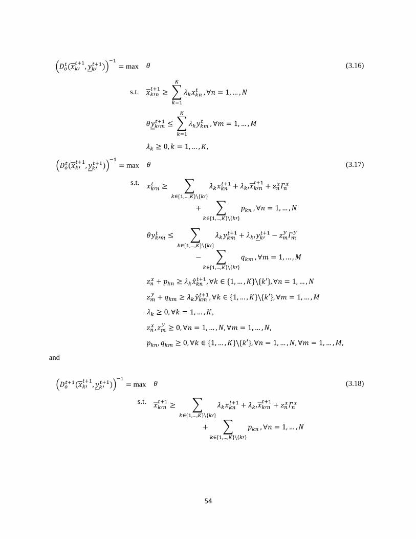
54
(𝐷𝑜𝑡(𝑥𝑘′
𝑡+1, 𝑦𝑘′𝑡+1))
−1= max 𝜃 (3.16)
s.t. 𝑥𝑘′𝑛𝑡+1
≥ ∑ 𝜆𝑘𝑥𝑘𝑛𝑡
𝐾
𝑘=1
, ∀𝑛 = 1,… ,𝑁
𝜃𝑦𝑘′𝑚𝑡+1 ≤ ∑ 𝜆𝑘𝑦𝑘𝑚
𝑡
𝐾
𝑘=1
, ∀𝑚 = 1,… ,𝑀
𝜆𝑘 ≥ 0, 𝑘 = 1,… , 𝐾,
(𝐷𝑜𝑡(𝑥𝑘′
𝑡+1, 𝑦𝑘′𝑡+1))
−1= max 𝜃 (3.17)
s.t. 𝑥𝑘′𝑛𝑡 ≥ ∑ 𝜆𝑘𝑥𝑘𝑛
𝑡+1
𝑘∈{1,…,𝐾}\{𝑘′}
+ 𝜆𝑘′𝑥𝑘′𝑛𝑡+1
+ 𝑧𝑛𝑥𝛤𝑛
𝑥
+ ∑ 𝑝𝑘𝑛𝑘∈{1,…,𝐾}\{𝑘′}
, ∀𝑛 = 1,… ,𝑁
𝜃𝑦𝑘′𝑚𝑡 ≤ ∑ 𝜆𝑘𝑦𝑘𝑚
𝑡+1
𝑘∈{1,…,𝐾}\{𝑘′}
+ 𝜆𝑘′𝑦𝑘′𝑡+1 − 𝑧𝑚
𝑦𝛤𝑚𝑦
− ∑ 𝑞𝑘𝑚𝑘∈{1,…,𝐾}\{𝑘′}
, ∀𝑚 = 1,… ,𝑀
𝑧𝑛𝑥 + 𝑝𝑘𝑛 ≥ 𝜆𝑘�̂�𝑘𝑛
𝑡+1, ∀𝑘 ∈ {1,… , 𝐾}\{𝑘′}, ∀𝑛 = 1,… ,𝑁
𝑧𝑚𝑦+ 𝑞𝑘𝑚 ≥ 𝜆𝑘�̂�𝑘𝑚
𝑡+1, ∀𝑘 ∈ {1,… , 𝐾}\{𝑘′}, ∀𝑚 = 1,… ,𝑀
𝜆𝑘 ≥ 0, ∀𝑘 = 1,… , 𝐾,
𝑧𝑛𝑥 , 𝑧𝑚
𝑦≥ 0, ∀𝑛 = 1,… ,𝑁, ∀𝑚 = 1,… ,𝑁,
𝑝𝑘𝑛, 𝑞𝑘𝑚 ≥ 0,∀𝑘 ∈ {1,… , 𝐾}\{𝑘′}, ∀𝑛 = 1,… ,𝑁, ∀𝑚 = 1,… ,𝑀,
and
(𝐷𝑜𝑡+1(𝑥𝑘′
𝑡+1, 𝑦𝑘′𝑡+1))
−1= max 𝜃 (3.18)
s.t. 𝑥𝑘′𝑛𝑡+1
≥ ∑ 𝜆𝑘𝑥𝑘𝑛𝑡+1
𝑘∈{1,…,𝐾}\{𝑘′}
+ 𝜆𝑘′𝑥𝑘′𝑛𝑡+1
+ 𝑧𝑛𝑥𝛤𝑛
𝑥
+ ∑ 𝑝𝑘𝑛𝑘∈{1,…,𝐾}\{𝑘′}
, ∀𝑛 = 1,… ,𝑁

55
𝜃𝑦𝑘′𝑚𝑡+1 ≤ ∑ 𝜆𝑘𝑦𝑘𝑚
𝑡+1
𝑘∈{1,…,𝐾}\{𝑘′}
+ 𝜆𝑘′𝑦𝑘′𝑚𝑡+1 − 𝑧𝑚
𝑦𝛤𝑚𝑦
− ∑ 𝑞𝑘𝑚𝑘∈{1,…,𝐾}\{𝑘′}
, ∀𝑚 = 1,… ,𝑀
𝑧𝑛𝑥 + 𝑝𝑘𝑛 ≥ 𝜆𝑘 �̂�𝑘𝑛
𝑡+1, ∀𝑘 ∈ {1,… , 𝐾}\{𝑘′}, ∀𝑛 = 1,… ,𝑁
𝑧𝑚𝑦+ 𝑞𝑘𝑚 ≥ 𝜆𝑘 �̂�𝑘𝑚
𝑡+1, ∀𝑘 ∈ {1,… , 𝐾}\{𝑘′}, ∀𝑚 = 1,… ,𝑀
𝜆𝑘 ≥ 0, ∀𝑘 = 1,… , 𝐾,
𝑧𝑛𝑥 , 𝑧𝑚
𝑦≥ 0, ∀𝑛 = 1,… ,𝑁, ∀𝑚 = 1,… ,𝑁,
𝑝𝑘𝑛, 𝑞𝑘𝑚 ≥ 0,∀𝑘 ∈ {1,… , 𝐾}\{𝑘′}, ∀𝑛 = 1,… ,𝑁, ∀𝑚 = 1,… ,𝑀.
Similarly, the upper productivity limit is defined as
𝑀𝑜(𝑥𝑘′𝑡 , 𝑦𝑘′
𝑡 , 𝑥𝑘′𝑡+1, 𝑦𝑘′
𝑡+1) = √
𝐷𝑜𝑡(𝑥𝑘′
𝑡+1, 𝑦𝑘′𝑡+1)
𝐷𝑜𝑡(𝑥𝑘′
𝑡 , 𝑦𝑘′𝑡 )
𝐷𝑜𝑡+1(𝑥𝑘′
𝑡+1, 𝑦𝑘′𝑡+1)
𝐷𝑜𝑡+1(𝑥𝑘′
𝑡 , 𝑦𝑘′𝑡 )
. (3.19)
Theorem 3.2 The upper productivity limit is greater than or equal to the lower productivity limit:
𝑀𝑜(𝑥𝑘′𝑡 , 𝑦𝑘′
𝑡 , 𝑥𝑘′𝑡+1, 𝑦𝑘′
𝑡+1) ≥ 𝑀𝑜 (𝑥𝑘′
𝑡 , 𝑦𝑘′𝑡 , 𝑥𝑘′
𝑡+1, 𝑦𝑘′𝑡+1).
The lower productivity bound (3.15) yields the minimum productivity where a DMU is assumed to
radially produce less output with more input, while only a restricted number of sites performs at its
estimated bound. Similarly, the upper bound is calculated by (3.19), with an estimate of more input and less
output for the next period from the DMU. Bounds for EC and TC are constructed in a similar fashion, using
the estimated distance functions.
3.4 An Application of Community Youth Prevention Programs
This section illustrates the proposed approach using the data from a real community youth
prevention program. We begin with an overview of the selected intervention program and acquisition of
data. Input and output variables collected throughout the lifetime of the program will be explained. Among
the input and output variables, we first select key variables based on the selective DEA model. Using

56
selected variables, we perform an evaluation of the productivity of all providers and present a monitoring
scheme for the time-varying efficiency of the sites.
3.4.1 Data and variables
The data set used in this study was obtained from one of three well-established intervention
programs supported by the Evidence-based Prevention and Intervention Support Center (EPISCenter), a
collaborative partnership between the Pennsylvania Commission on Crime and Delinquency (PCCD) and
the Prevention Research Center at Penn State University.1 Among the menu of evidence-based prevention
and intervention programs served by EPISCenter, we single out one intervention program that focuses on
youth with behavioral offenses and substance abuse, and addresses the acting-out behavior of youth by
improving family functioning. Intervention is typically conducted in family’s home by a trained therapist
as a home-based model. A team accepts dysfunctional or at-risk youth aged 11-18 and their families in the
treatment process and delivers the program over 3-5 months through qualified therapists. On average, a
small site of two full-time therapists for the community-based program serves 90 youths per year, while a
large site with eight clinicians can server almost 300 clients per year.
Data in this study comes from the INtegrated System for Program Implementation and Real-time
Evaluation (INSPIRE), a web-based data collection and reporting system, developed by the Penn State
College of Engineering and EPISCenter with funding from PCCD. The system enables providers to easily
collect, store, document, analyze and report data, and facilitates model fidelity and successful outcomes
across providers. Data in INSPIRE comes from two sources: regular import of national data on the program
and direct data entry from therapists using a web-based interface. Variables in the database include
demographic information on youth, treatment outcomes, and provider-level information. A report is
generated periodically to summarize the treatment outcomes of youths, including youth and family
satisfaction about the program experience, improved family functioning, successful discharge rate,
1 For more information, please refer to the EPISCenter at http://www.episcenter.psu.edu/.

57
successful completion rate, and the number of youth who remain drug-free, avoid re-arrest, show no new
offenses, remain in the community, and improve school attendance and performance.
Among the outcome variables, we select some key variables to evaluate longitudinal productivity,
as summarized in Table 3.1. The set of input variables contains the number of participants: number of youth
served, number of new enrollments, and number of new families. The output variables include the number
of discharged cases (number of youth discharged) and outcomes at discharge (percentage of youths
successfully discharged, percentage of youths who complete the program, percentage of youths with no
new offenses, percentage of youths remaining in the community, and percentage of youths improving
family functioning).
Table 3.1 Variables
N1 Number of youth served
N2 Number of new youth enrolled
N3 Number of new parents enrolled
N4 Number of youth clinically discharged
N5 Number of therapists with Global Therapist Review (GTR)
N6 Number of therapists satisfying minimum fidelity standards
N7 Number of therapists satisfying minimum adherence standards
P1 Percentage of youth satisfied
P2 Percentage of families satisfied
P3 Percentage of youth who completed the program
P4 Percentage of successful discharges
P5 Percentage of youth with no new offenses
P6 Percentage of youth living in community
P7 Percentage of youth improving school attendance
P8 Percentage of youth improving academic performance
P9 Percentage of families with improved functioning

58
Note that N1 counts the total number of cases open and active during the period, and hence one
youth can be counted multiple times in different periods until s/he completes the program. Variables N2
and N3 are the number of referred youth and families who enroll in the program and have a first session
during the period. N4 counts only youth who are clinically discharged, that is, youth with the opportunity
to complete treatment, who are not discharged for administrative reasons unrelated to case progress.
Variables N5 through N7 are related to implementation quality, demonstrating the qualification of therapists
who complete required training and certification. Site supervisors complete weekly ratings of therapist
fidelity (N5) and dissemination adherence (N6), and these ratings are averaged to Global Therapist Review
(GTR) (N7) three times a year.
P1 and P2 are the percentage of youth and families who make positive answers in questionnaires
on the program. P3 measures the rate of discharges among youths who completed treatment, while P4
measures the rate of successful discharges. Percentage variables P5 through P9 are performance measures
of proximal outcomes for all clinically discharged youth. P5 indicates decreases in delinquent behavior and
general behavior problems, while P6 is the percentage of youth living in the community at discharge.
School-related measures P7 and P8 indicate positive results in school attendance and performance,
respectively, but only include youth presenting with concerns in those areas at enrollment. As an indicator
of improvement in family functioning, P9 reports increased family communication and cohesion, and less
verbal aggression and conflict.

59
Table 3.2 Input and output variables by quarter
FY Quarter N1 N2 N3 N4 P1 P2 P3 P4 N5 N6 N7 P5 P6 P7 P8 P9
2010
1 713 344 0 279 81.3 68.8 71.0 59.1 14 9 12 78.5 88.5 20.0 0.0 70.4
2 716 321 0 317 90.9 90.9 71.6 54.3 23 15 20 75.9 87.4 33.3 75.0 60.9
3 655 307 0 283 76.5 94.1 66.8 55.5 24 16 22 83.9 85.5 40.0 33.3 66.1
4 694 350 0 277 90.9 94.3 77.6 63.2 27 17 23 82.7 88.1 68.8 52.6 69.1
Total 1691 1322 0 1156 87.9 90.9 71.7 57.9 42 25 35 80.0 87.4 57.8 47.2 66.3
2011
1 627 259 0 248 93.8 96.0 75.8 64.9 24 14 19 87.5 91.9 60.0 61.5 72.5
2 621 288 0 237 93.3 96.2 67.1 59.1 39 25 30 82.9 89.0 62.5 66.0 63.0
3 618 271 266 254 88.5 91.4 76.4 67.3 29 23 24 81.0 88.2 60.5 64.9 69.9
4 554 238 162 234 91.4 94.0 80.8 73.1 17 16 14 89.0 91.9 63.2 63.5 73.6
Total 1424 1056 891 973 91.4 94.1 75.0 66.1 51 32 36 85.0 90.2 61.8 64.2 69.9
2012
1 530 248 188 206 91.4 93.6 82.5 79.6 25 19 24 89.7 91.3 58.3 68.2 77.3
2 508 223 197 177 94.2 93.0 75.7 67.2 36 20 31 84.1 86.4 59.3 61.5 78.4
3 555 254 210 198 89.4 89.3 78.3 72.2 19 12 17 87.8 89.9 67.7 72.7 78.7
4 585 273 301 186 89.9 89.9 76.9 69.9 21 16 18 85.0 90.9 71.0 65.9 70.6
Total 1280 998 896 767 91.0 91.2 78.5 72.5 41 22 33 86.8 89.7 64.6 67.6 76.2
2013
1 595 250 216 208 92.1 94.4 83.2 74.5 16 14 16 89.7 93.3 69.0 68.3 78.3
2 561 210 213 230 88.7 94.3 80.0 72.6 14 12 12 87.6 92.2 53.7 45.9 69.2
3 523 227 248 181 83.8 88.0 69.6 62.4 12 9 8 81.5 89.5 51.4 43.2 61.9
4 555 236 281 211 85.4 91.0 72.5 66.4 33 25 29 88.8 88.6 58.0 55.4 66.3
Total 1268 923 958 830 87.7 92.1 76.6 69.3 38 28 33 87.1 91.0 58.8 53.9 69.2
2014
1 552 243 274 208 96.6 95.2 75.5 72.6 34 23 32 86.2 89.9 63.3 50.0 73.6
2 526 207 233 204 94.2 94.8 78.4 73.5 10 8 10 88.5 90.2 60.4 67.7 70.2
3 499 213 239 171 97.4 96.6 83.0 76.6 14 12 9 89.7 90.6 53.9 53.3 75.6
4 514 221 220 172 93.8 93.8 83.7 79.1 22 20 20 89.9 93.6 74.1 70.0 77.8
Total 1193 884 966 755 95.5 95.1 79.9 75.2 45 35 36 88.5 91.0 62.7 60.1 74.1
2015
1 544 233 247 191 88.4 89.2 76.4 70.2 19 19 17 85.9 90.6 54.6 54.4 69.8
2 522 197 186 176 95.2 94.4 83.0 81.3 9 9 9 87.9 90.3 58.8 63.2 70.2
3 525 205 201 188 90.3 95.6 78.2 76.1 21 17 19 88.0 91.0 73.7 70.0 72.1
4 519 213 193 149 92.3 94.4 77.2 70.5 12 11 12 85.5 89.9 72.2 57.1 68.7
Total 1159 848 827 704 91.5 93.2 78.7 74.6 30 27 26 86.9 90.5 61.7 61.2 70.3

60
We will refer to quarterly data on the prevention program from the first quarter of FY 2010, starting
on 1 July 2010 and including data through the last quarter of FY 2015, ending June 30 2016. Analysis of
time-dependent efficiency is based on the total 16 sites that implemented the prevention program during
that period. Not all sites were active during the whole period: some of them stopped operating upon
termination of funding, while others started the program in the middle of the period. Table 3.2 presents
statistics on the data over the period. The quarterly data indicate that the number of participants in the
program gradually decreases as N1 and N2 decrease over the years. Served by 10.17 opening sites on
average, the six-year averages of N1 and N2 are 575.46 and 251.29, respectively. Similarly, N4 declines
over the period, with a six-year average of 216.04 youths. Note that there is no N3 data for the first six
quarters, but we do not know whether this is because the data were not collected properly or simply because
there were no new families during the period.
Figure 3.4 Desired clinical discharges

61
Figure 3.5 Proximal outcomes at discharge
Completion rate (P3) reflects the percentage of clinically discharged youth who completed the
program, while the rate of successful discharge (P4) is the percentage of youth whose discharge outcome
is successful among completers. Over the six-year period, among 5,185 youth who were clinically
discharged from the program, 3,954 youth (76.3%) completed the three phases of the program and 3,536
youth (68.2%) were successfully discharged. Figure 3.4 demonstrates that across providers, quarterly
average P3 and P4 ranged from 66.8% to 83.7% and from 54.3% to 81.3%, respectively during the six fiscal
years.
Figure 3.5 presents treatment outcomes reported for all clinically discharged youth. While P5 and
P6 are measures of youth who had concerns at intake, and indicate achievement of goals at a relatively high
rate, the other three indicators, P7, P8, and P9, for improved academic attendance/performance and family
functioning, fluctuate at lower percentages. Moreover, P7 and P8 show similar tendencies, indicating that
school attendance and academic performance are highly correlated.

62
3.4.2 Results
The data set presents some challenging issues. First, there is no consensus as to the key input and
output variables. Furthermore, there are some variables with zeroes, partly because the variable entry is
mainly dependent on the data entry by therapists through the system. The efficiency scores obtained from
such data may be less reliable than scores from more complete data. Technically speaking, when the number
of performance measures is relative large compared to the number of active sites there is a problem
involving degrees of freedom and relative efficiency. The following rule of thumb for the envelopment
model is suggested by Cooper et al. (2007).
𝐾 ≥ max{3(𝑀 +𝑁),𝑀𝑁}. (3.20)
To address these issues we start by identifying key input and output variables using the selective
DEA model proposed by Toloo et al. (2015). They suggest an MILP model by imposing the maximum
number of input and output variables holds the condition. Assuming that selecting N2 as an input variable
is inevitable, we apply the selective model for each quarter. Given that the number of sites satisfying 𝐾 ≥
3 (𝑀 + 𝑁), we solve the following selective DEA model that maximizes the aggregate efficiency:
max𝝁,𝝂
𝜃 = ∑ 𝜇𝑚�̃�𝑚
𝑀
𝑚=1
(3.21)
s. t. ∑𝑣𝑛�̃�𝑛
𝑁
𝑛=1
= 1
∑ 𝜇𝑚𝑦𝑘𝑚
𝑀
𝑚=1
≤ ∑𝑣𝑛𝑥𝑘𝑛
𝑁
𝑛=1
∀𝑘 = 1,… , 𝐾
∑ 𝑞𝑚
𝑀
𝑚=1
+∑𝑝𝑛
𝑁
𝑛=1
≤ ⌊𝐾
3⌋
∑ 𝑞𝑚
𝑀
𝑚=1
≥ 1

63
𝜖𝑝𝑛 ≤ 𝜈𝑛 ≤ 𝐿𝑝𝑛 ∀𝑛 = 1,… ,𝑁
𝜖𝑞𝑚 ≤ 𝜇𝑚 ≤ 𝐿𝑞𝑚 ∀𝑚 = 1,… ,𝑀
𝜈𝑛 ≥ 𝜖 ∀𝑛 = 1,… ,𝑁
𝜇𝑚 ≥ 𝜖 ∀𝑚 = 1,… ,𝑀
𝑝𝑛 ∈ {1,0} ∀𝑛 = 1,… ,𝑁
𝑞𝑚 ∈ {1,0} ∀𝑚 = 1,… ,𝑀,
where �̃�𝑛 = ∑ 𝑥𝑘𝑛𝐾𝑘=1 ∀𝑛 = 1,… ,𝑁, �̃�𝑚 = ∑ 𝑦𝑘𝑚
𝐾𝑘=1 ∀𝑚 = 1,… ,𝑀, 𝐿 is a large positive number and 𝜖 is
a small positive faction number. Binary variables 𝑝𝑛 and 𝑞𝑚 indicate whether input variable n or output
variable m is selected or not, respectively. The third constraint ensures that the optimal selection of input
and output variables does not exceed ⌊𝐾 3⁄ ⌋, which leads to satisfaction of formulation (3.20). With the
average aggregated efficiency score being 0.71, N1 and N4 are determined as selective input and output
variables, as those variables are most frequently selected.
Table 3.3 Comparative efficiency by fiscal year
Before applying selective model After selecting variables
FY No. Active Sites No. Eff. Sites Avg. Eff. No. Eff. Sites Avg. Eff.
2010 12 8 0.9565 1 0.8533
2011 12 6 0.9251 2 0.7778
2012 10 5 0.8963 1 0.7887
2013 11 5 0.9424 2 0.8396
2014 11 6 0.9166 1 0.7229
2015 9 9 1.0000 1 0.9105
Total 65 39 0.9395 8 0.8155

64
Figure 3.6 Yearly average efficiency scores of sites
Table 3.3 presents the number of efficient sites and year-by-year efficiency obtained for each of
the six fiscal years. Given the selection of input and output variables, the efficiency score seems more
reasonable, with a six year average of 0.82 compared to the average 0.94 without selecting variables.
Overall, approximately 12.3% of the sites (8 of the total 65 active sites) are evaluated as efficient, while
60% (39 out of 65 active sites) were recognized as efficient before applying the selective model. The overall
average efficiency score of all 65 sites for the period is 0.82, which implies that given the level of inputs,
sites should have increased their output by 18% proportionally in order to be efficient. In this specific case,
since the number of clinical discharges is the only selected output, sites should have achieved more clinical
discharges for a given number of enrollments and number served. Over the six-year time span, the
aggregated efficiency score of the program presents a sequence with a weak increasing trend. As shown in
the dashed line in Figure 3.6, the change in efficiency is slightly positive over the period, with the largest
efficiency in FY 2015. After dropping significantly in the second fiscal year, the score displays
improvement, except for relatively poor performance in FY 2014.

65
To assess productivity growth over time, we need to investigate quarter-by-quarter evaluations. We
calculated the Malmquist productivity indices including the efficiency change and technical change
components by quarter. Instead of using yearly aggregated data, we used quarterly data on the prevention
program over time. For each consecutive two-quarter period, four linear programming (LP) models were
solved to obtain distance functions as described in the previous section. (In other words, we calculate 1,120
LP models in total using CPLEX v.12.2.) We then take a geometric mean for each site index to evaluate
cumulated productivity, cumulated efficiency change, and cumulated technical change.
Figure 3.7 Cumulated results of Malmquist productivity index
Table 3.4 Average annual productivity growth of the youth prevention program over FY 2010-FY 2015
Year MPI EC TC

66
FY 2010 1.0216 0.9960 1.0256
FY 2011 1.0295 1.0925 0.9423
FY 2012 1.0482 1.0574 0.9912
FY 2013 1.0421 1.0176 1.0241
FY 2014 1.0440 1.0516 0.9927
FY 2015 1.0049 0.9940 1.0109
Average 1.0327 1.0346 0.9981
Figure 3.7 illustrates cumulated changes for MPI, EC, and TC for entire program. Average annual
changes of those components are summarized in Table 3.4. Overall, MPI increased by 120.62% over a 6-
year period, with geometric mean of 3.27% a year. EC increased 140.58% over the 6-year period, with
geometric mean of 3.46% a year, but changes in TC were small. In fact, TC decreased over the 6-year
period by 8.30%. These results show that a significant component of the growth in productivity was due to
improvement in efficiency level (EC), rather than innovation (TC).
Table 3.5 Average quarterly changes by site
Site MPI EC TC Rank
Site-01 0.9850 0.9938 0.9911 13
Site-02 1.0533 1.0000 1.0533 8
Site-03 1.0093 1.0072 1.0021 9
Site-04 1.1094 1.0228 1.0847 4
Site-05 0.9766 1.0297 0.9484 15
Site-06 0.9757 0.9821 0.9935 16
Site-07 0.9929 0.9983 0.9946 12
Site-08 1.1010 1.1226 0.9808 5
Site-09 0.9952 0.9949 1.0004 11
Site-10 0.9986 1.0204 0.9787 10
Site-11 0.9809 0.9966 0.9842 14

67
Site-12 1.3664 1.3681 0.9987 2
Site-13 1.0975 1.1213 0.9727 6
Site-14 1.2913 1.1937 1.0730 3
Site-15 1.6355 1.6407 0.9969 1
Site-16 1.0951 1.1500 0.9822 7
To give some idea of the productivity of an individual program provider, we turn to average
quarterly results for each site. Table 3.5 exhibits the average productivity, average efficiency change and
average technical change components for each site over the entire FY 2010 – FY 2015 time period. The
results tell another story about productivity growth. At some sites, changes in productivity were due to
efficiency change (EC) rather than technology shift (TC), but the pattern was different at other sites. For
instance, the productivity changes of sites such as Site-02, Site-12 and Site-15 were largely due to the
innovation (TC); at other sites improvements in both efficiency and technology shift made an impact on the
productivity. Site-12, Site-14, and Site-15 were the three top performers in terms of productivity, but not
all of them were good at shifting the frontier. In fact, the rate of technology change of Site-14 was second
highest, but technology change regressed (TC < 1) at the other two sites.
Overall, the technical change (TC) component given in Table 3.5 signifies a shift in frontier
technology for each country, but the average results do not fully identify which site actually causes the
technical frontier to shift between period 𝑡 and 𝑡 + 1. Färe et al. (1994) suggested a set of criteria to identify
the “innovators” that contribute to the frontier shift over the pair of periods. In addition to TC greater than
1, the criteria include two distance functions for period 𝑡 + 1. The innovators classified by these conditions
are shown in the second column of Table 3.6.
Table 3.6 Sites shifting the technology frontier
Period Innovators Disruptive
innovators
Sustaining
innovators

68
FY10 Q1-FY10 Q2 Site-03, Site-05 Site-03 Site-05
FY10 Q2-FY10 Q3 - - -
FY10 Q3-FY10 Q4 - - -
FY10 Q4-FY11 Q1 Site-07, Site-04 Site-07, Site-04 -
FY11 Q1-FY11 Q2 - - -
FY11 Q2-FY11 Q3 Site-10 Site-10 -
FY11 Q3-FY11 Q4 Site-10 Site-10 -
FY11 Q4-FY12 Q1 - - -
FY12 Q1-FY12 Q2 Site-14 Site-14 -
FY12 Q2-FY12 Q3 Site-09, Site-10 Site-09, Site-10 -
FY12 Q3-FY12 Q4 Site-06, Site-14 Site-06, Site-14 -
FY12 Q4-FY13 Q1 Site-02 Site-02 -
FY13 Q1-FY13 Q2 Site-11 - Site-11
FY13 Q2-FY13 Q3 Site-14 Site-14 -
FY13 Q3-FY13 Q4 - - -
FY13 Q4-FY15 Q1 Site-11, Site-16 Site-16 Site-11
FY14 Q1-FY14 Q2 Site-14 Site-14 -
FY14 Q2-FY14 Q3 - - -
FY14 Q3-FY14 Q4 Site-16 Site-16 -
FY14 Q4-FY15 Q1 - - -
FY15 Q1-FY15 Q2 - - -
FY15 Q2-FY15 Q3 Site-01, Site-16 Site-01 Site-16
FY15 Q3-FY15 Q4 Site-03 Site-03 -
To delve deeper into the shift in the technology frontier over time, we further look at the robust
productivity bound. For each site, we construct upper and lower limits of the robust productivity bound
based on the most and least favorable estimates of period 𝑡 + 1, respectively. Using the chart, we can
monitor the quarterly trend of average performance over time and control the quality of prevention service

69
delivery. Assuming proportional changes, we estimate the upper limit for period 𝑡 + 1 where the input
decreases by 𝛼 and output increases by 𝛼 from period 𝑡. Namely,
𝑥𝑘′𝑛𝑡+1 = (1 − 𝛼)𝑥𝑘′𝑛
𝑡 ∀𝑛 = 1,… ,𝑁, (3.22)
𝑦𝑘′𝑚𝑡+1
= (1 + 𝛼)𝑦𝑘′𝑚𝑡 ∀𝑚 = 1,… ,𝑀, (3.23)
𝑥𝑘𝑛𝑡+1 ∈ [ (1 − 𝛼)𝑥𝑘𝑛
𝑡 , (1 + 𝛼)𝑥𝑘𝑛𝑡 ] ∀𝑘 ∈ {1,… , 𝐾}\{𝑘′}, ∀𝑛 = 1,… ,𝑁, (3.24)
and
𝑦𝑘𝑚𝑡+1 ∈ [ (1 − 𝛼)𝑦𝑘𝑚
𝑡 , (1 + 𝛼)𝑦𝑘𝑚𝑡 ] ∀𝑘 ∈ {1,… , 𝐾}\{𝑘′}, ∀𝑚 = 1,… ,𝑀. (3.25)
The lower limit is estimated using a similar (opposite) method. As explained in the previous section,
the lower productivity bound can be achieved when a site has fewer discharge cases with more active
participants and new enrollments, and the upper bound can be achieved in the opposite case.

70
Figure 3.8 Robust productivity bound and productivity index
Figure 3.8 depicts the average productivity index and its bounds with 𝛼 = 0.1. While most of the
productivity index points fall within the bounded interval, there are some data points that are “out-of-
control.” To interpret such nonrandom patterns, we identify “disruptive innovators” based on the
component distance function and technology change index exceeding their upper bound. Specifically, if
TC > max{TC, 1}, (3.26)
𝐷𝑜𝑡(𝑥𝑘′
𝑡+1, 𝑦𝑘′𝑡+1) > max {𝐷𝑜
𝑡(𝑥𝑘′𝑡+1, 𝑦𝑘′
𝑡+1), 1} (3.27)
and
𝐷𝑜𝑡+1(𝑥𝑘′
𝑡+1, 𝑦𝑘′𝑡+1) = 1, (3.28)
then site 𝑘′ makes a disruptive shift in the technology frontier between periods 𝑡 and 𝑡 + 1. As innovations
from such sites are far larger than those of other sites in the program, they may cause disruption for the rest
of the sites. This tends to happen when a new site enters the system and preserves its advantage in the early
stage. This is because an established site can serve more participants and possibly release more, but the

71
number of discharges tends to be diminished as program implementation becomes mature and finally winds
up due to contract termination. We distinguish innovators that are not disruptive and make a frontier shift
by sustaining productivity. The third and fourth columns in Table 3.6 represent a list of sites that make
disruptive and sustaining innovations, respectively.

72
Table 3.7 Detailed components information associated with upper and lower limits
Site Index FY10 FY11 FY12 FY13 FY14 FY15
Q1 Q2 Q3 Q4 Q1 Q2 Q3 Q4 Q1 Q2 Q3 Q4 Q1 Q2 Q3 Q4 Q1 Q2 Q3 Q4 Q1 Q2 Q3
01 MPI > < > < > - - - < - > - - - - < > - - - - > <
EC - < > < > < < > < < - - - < - < - - < > - - <
TC > - < > < > > < - - > - > > - > > < > < - > -
02 MPI - < - - - < - > < > < > < < > - - < > N/A N/A N/A N/A
EC < < > < > < < > < > < > - < > - < - - N/A N/A N/A N/A
TC > - < > < > > < - > > > < - - > > < > N/A N/A N/A N/A
03 MPI > < - - < - - > - < - - < - < > < > < > < > >
EC - < - < < - < > - < - - < - < > < > < > < > >
TC > - < > < > > < - - > - > > - > > < > < - > >
04 MPI - > < > N/A N/A N/A N/A N/A N/A N/A N/A N/A N/A N/A N/A N/A N/A N/A N/A N/A N/A N/A
EC < - < - N/A N/A N/A N/A N/A N/A N/A N/A N/A N/A N/A N/A N/A N/A N/A N/A N/A N/A N/A
TC > - - > N/A N/A N/A N/A N/A N/A N/A N/A N/A N/A N/A N/A N/A N/A N/A N/A N/A N/A N/A
05 MPI > < - - > N/A N/A N/A N/A N/A N/A N/A N/A N/A N/A N/A N/A N/A N/A N/A N/A N/A N/A
EC - < > < > N/A N/A N/A N/A N/A N/A N/A N/A N/A N/A N/A N/A N/A N/A N/A N/A N/A N/A
TC > - < > < N/A N/A N/A N/A N/A N/A N/A N/A N/A N/A N/A N/A N/A N/A N/A N/A N/A N/A
06 MPI - - - - > - < - - - > < - < > - - - - > - - <
EC < - - < > < < - - < - < - < > < < - < > - < <
TC > - < > < > > < - - > - > > - > > < > < - > -
07 MPI - - - > < > > < - > < > - - < > < - < > < - -
EC < - - - < - - - - - < > < - < > < > < > < - <
TC > - < > < > > < - - > - - > - > > < > < - > -
08 MPI > < > N/A N/A N/A N/A N/A N/A N/A N/A N/A N/A N/A N/A N/A N/A N/A N/A N/A N/A N/A N/A
EC - < > N/A N/A N/A N/A N/A N/A N/A N/A N/A N/A N/A N/A N/A N/A N/A N/A N/A N/A N/A N/A
TC > - < N/A N/A N/A N/A N/A N/A N/A N/A N/A N/A N/A N/A N/A N/A N/A N/A N/A N/A N/A N/A
09 MPI - - < - - - > - < > < < > - - < > < - < > < <
EC < - - < > < - - < > < < > < - < > - < > > < <
TC > - < > < > > < - > - - > > - > > < > < - - -
10 MPI - - - > < > > < - > < > - > - - - - N/A N/A N/A N/A N/A
EC < - - - < - - < - > < > - > < - < > N/A N/A N/A N/A N/A
TC > - < > < > > < - > - - > > - > > < N/A N/A N/A N/A N/A
11 MPI < > - - < > > < > - < > > < - > < - > < > - >
EC < > - < < - - < > < < > > < - - < > < > > < -
TC - - < > < > > < > - > - > - - > > < > < - > -

73
12 MPI > > - < > - N/A N/A N/A N/A N/A N/A N/A N/A N/A N/A N/A N/A N/A N/A N/A N/A N/A
EC > > - < > < N/A N/A N/A N/A N/A N/A N/A N/A N/A N/A N/A N/A N/A N/A N/A N/A N/A
TC > - < > < > N/A N/A N/A N/A N/A N/A N/A N/A N/A N/A N/A N/A N/A N/A N/A N/A N/A
13 MPI N/A N/A N/A N/A N/A N/A N/A N/A > < - > - < > < - > < - - - <
EC N/A N/A N/A N/A N/A N/A N/A N/A > < < > - < > < < > < > < - <
TC N/A N/A N/A N/A N/A N/A N/A N/A - - > - - > - - > < > < - > -
14 MPI N/A N/A N/A N/A N/A N/A > < > < > < > > < < > N/A N/A N/A N/A N/A N/A
EC N/A N/A N/A N/A N/A N/A > - > < > < > - - < > N/A N/A N/A N/A N/A N/A
TC N/A N/A N/A N/A N/A N/A > < > - > - > > - - > N/A N/A N/A N/A N/A N/A
15 MPI N/A N/A N/A N/A N/A N/A N/A N/A N/A N/A N/A N/A N/A N/A N/A N/A N/A N/A N/A N/A > < >
EC N/A N/A N/A N/A N/A N/A N/A N/A N/A N/A N/A N/A N/A N/A N/A N/A N/A N/A N/A N/A > < >
TC N/A N/A N/A N/A N/A N/A N/A N/A N/A N/A N/A N/A N/A N/A N/A N/A N/A N/A N/A N/A - > -
16 MPI N/A N/A N/A N/A N/A N/A N/A N/A N/A N/A N/A N/A N/A N/A > > - < > - < > <
EC N/A N/A N/A N/A N/A N/A N/A N/A N/A N/A N/A N/A N/A N/A > > < - < > < > <
TC N/A N/A N/A N/A N/A N/A N/A N/A N/A N/A N/A N/A N/A N/A > > > < > < - > -

74
Table 3.7 reports the detailed component information associated with its bounds. The greater than
sign (>) shows where the actual index is greater than both 1 and the estimated upper limit, while the less
than sign (<) implies that the actual index is less than the estimated lower limit. This approach helps to keep
the system within an acceptable level of productivity by identifying repeated patterns. If a sequence of data
points falls below the lower limit (or above the upper limit), we can detect a significant deterioration (or
suspicious false-positivity) in productivity. For instance, component TC of Site-02 exceeds its upper bound
in three consecutive quarters during FY12 Q2 – FY12 Q4, and Site-16 does the same from FY13 Q3 to
FY14 Q1. Both exceptions show disruptive innovations in the following periods, as shown in Table 3.6.
Ideally, we can avoid harmful situations by early detection and notification of an exception.
3.5 Implementation and Integration of Monitoring Engine
The proposed approach can be incorporated as a key element of an enhanced data-driven system.
With the current INSPIRE database we described earlier as a foundation, the approach we proposed earlier
can be integrated into the new data-driven system. First, it will provide an automatic end-of-period outcome
analysis and performance evaluation based on it. The monitoring engine will detect deviations based on the
productivity index and generate alerts for appropriate prevention personnel accordingly. The event will be
driven by the significance of deviation from the estimation of the implementation plan. For instance, when
the negative productivity patterns are repeated in three consecutive periods, we can detect a significant
deterioration in productivity. The system issues an alert message to the prevention service providers, such
as practitioners or local site administrators, so that they can recognize explicitly where the exception occurs
and which outcome they need to promote. This will remove an ad hoc nature in prevention programs that
are being executed.
Furthermore, the monitoring engine can be aligned with the early waning functionality. Based on
the system warning for the possible abnormality of the productivity in the next period, program providers
can accommodate its resources in advance. They can concentrate their efforts on enhancing specific

75
outcome measure to avoid such situations. The productivity bound will be presented as a target value for
the goal they need to achieve in the following period.
Overall, this new environment can fundamentally transform the implementation of prevention
programs and eventually enhance the efficiency of prevention service delivery. Our approach can further
motivate an adoption of engineering tools and techniques in the prevention research, practice, and policy.
3.6 Conclusions
Stakeholders from community youth prevention programs call for appropriate measures of
statewide growth productivity of the programs as well as the efficiency of individual sites. There is a variety
of outcome variables for youth at discharge, but no common consent on measures of the efficiency of
program providers. In the present study, we introduce a robust productivity index approach that enables
periodic monitoring and early detection of exception. The upper and lower bounds can be interpreted as the
maximum and minimum achievable productivity of estimated performance for the following period. The
derivation of both limits is done by solving the robust version of the Malmquist productivity index.
We apply the proposed approach to performance data for a community youth program from FY
2010 to FY 2015, including data from both a national database and local practitioners. Analysis of MPI,
EC and TC shows that the total factor productivity of all sites increased by 120.62% from FY 2010 to FY
2015, and mainly driven by efficiency improvement rather than technological progress. Innovators that
caused the frontier shift are identified, and differentiated into two separate classes by investigating the
robust bound. The results from the robust productivity analysis also show that random occurrences of an
exception and significant patterns of productivity change can be detected and monitored. Ultimately, the
approach has the potential to become a decision support tool for prevention service providers, and permits
early identification (and thus elimination) of sources of exception.
It should be noted that the results of this empirical study are dependent upon the limited number of
input and output variables available, given the small number of sites running the program as compared to

76
the set of data available in the system. This study could be extended by covering a prevention program with
a larger number of sites, and including more relevant variables for better solution quality.

77
4 REAL-TIME SUPPLY CHAIN CONTROL USING ADAPTIVE WIP
ALGORITHM2
4.1 Introduction
In determining inventory levels of multistage supply chain and production system problems, it is
hard or even not feasible to obtain closed-form, analytic solutions, and hence computationally demanding
heuristic algorithms are often used to find the best inventory level. Moreover, less is known about the exact
effect of the inventory level of a single stage or subsystem, to the overall system performance and service
level of the supply chain. In this chapter, we provide a feedback algorithm that efficiently finds the best
inventory solution of the system, considering throughput, individual inventory level, and blocking parts.
The algorithm dynamically controls the three performance measures by adjusting the maximum level of
inventory in the subsystem.
The focus of this chapter is to show the representation of the adaptive feedback algorithm and study
the convergence and robustness of the algorithm. Feedback control is an efficient methodology to manage
dynamics of complex systems and has been applied to various production systems and inventory
management problems (Ortega and Lin 2004, Sarimveis et al., 2008). Target performance measure, which
is called a ‘command’, indicates a desired level and its value is compared to the one from simulation runs.
Based on the difference between the command and feedback value, a ‘controller’ makes corrective actions
to the system and manipulation is adjusted through an ‘actuator’. Given the target level of throughput of
the system, we choose two additional commands, Work-In-Process (WIP) levels and blocking time. As the
iteration runs, the algorithm dynamically changes the inventory levels and finds the inventory level in each
of the subsystem.
In pull manufacturing systems, such as Kanban and CONWIP, production timing and release of
raw materials are synchronized and controlled by the ‘cards’. Upon the departure of a job at the end of the
2 The AWIP algorithm is originally suggested by Masin and Prabhu (2005)

78
subsystem, the card is released and sent back to the initial point, so that it indicates there is available space
for the new arrival of the next job. Therefore, the number of cards in the subsystem governs production
activities and finding the optimal number of cards makes a significant impact on performances of the overall
system. If the number of cards is too low, then not enough parts can be processed in the subsystem and the
throughput level may not be desirable. On the other hand, if too many parts are allowed in the card loop,
then one may suffer from large inventory costs. Therefore, we need to find the best number of cards that
tradeoff between WIP level and throughput.
The rest of this chapter is organized as follows. In Section 4.2, we provide a review of the literature
of relating to dynamic card controlling scheme of pull systems, and basic concepts of self-regulated
production systems. The Adaptive WIP (AWIP) algorithm design is illustrated in Section 4.3. In Section
4.4, experimental results are presented to show the dynamics of the algorithm, and compared to the results
of the mathematical problem. Finally, we discuss the conclusions and future works in Section 4.5.
4.2 Literature Review of Card Controlling System
4.2.1 Kanban and CONWIP system
With the adoption of Just-In-Time (JIT) principles, the Kanban system is one of the most well-
known pull manufacturing systems. As a medium of production information, Kanban cards authorize both
order quantity and production timing. Operation starts processing when both raw materials and Kanban
cards become available as the cards are released upon the departure of parts at the end of the production
stage. Therefore, the number of Kanban cards in each stage corresponds to the inventory level of the stage
because it dominates the work-in-process (WIP) level by capping the number of parts in that stage. One can
find the optimal number of cards in Kanban system, so as to minimize total costs including inventory
holding cost and backorders.
The Kanban system has its advantages because it is easy to optimize and runs effectively when
demand is stable. However, when a company experiences variabilities in demand or processing times, the
system needs to be redesigned by readjusting the parameter of the system. Rees et al. (1987) consider the

79
dynamic card control methods, where the number of cards matches current environmental conditions. Their
approaches are based on the demand forecast and statistical estimation of the lead time, but once the Kanban
level is readjusted, the system runs during the planning period. Gupta and Al-Turki (1997) suggest a flexible
Kanban system, a simple procedure to decide the number of additional cards needed. However, their
algorithm also requires the known demand and system capacity for the planning period. Therefore, both
methods are more of medium run planning, lacking the real-time reactive adjustment.
Takahashi and Nakamura (1996) and Takahashi and Nakamura (1999) explore the reactive JIT
control mechanism of the size of buffer allocation. The unstable changes in demand and production time is
absorbed in the buffers allocated to each inventory point. By monitoring time series data, the performances
of systems are analyzed based on the simulation results. The number of Kanban cards is intelligently
reallocated according to the previous simulation run, revealing the trade-off relationship of two
performance measures, the average waiting time of production demand and the total average WIP level.
Tardif and Maaseidvaag (2001) consider an adaptive method for a single stage Kanban system. Their
algorithm finds a set of optimal parameters for the Kanban cards and release and capture thresholds of
inventory level, and determines release and reorder points based on the current demand. It should be noted
that the single stage, one card Kanban system is equivalent to the CONWIP production system, stated below.
CONWIP production system is another pull manufacturing system that limits the total number of
jobs in the production line. The number of jobs in the system is usually governed by cards attached to the
jobs. When a job is processed in the last station, the card is detached and sent back to the beginning of the
system to be attached to the new job queueing at the first station. Therefore, the overall number of WIP in
the production line remains at constant (Spearman et al. 1990). In that sense, the card controlling mechanism
of the CONWIP system can be viewed as that of a single-stage Kanban system. The noticeable contribution
about the card controlling in CONWIP system can be seen in Hopp and Roof (1998) and Framinan et al.
(2006).

80
Hopp and Roof (1998) present a statistical control chart-based mechanism, where the number of
cards in the CONWIP line is dynamically adjusted based on the current system throughput. Intermediate
outputs of the current production line are evaluated and compared to the target throughput level or the
critical WIP level. When it falls below (or increase) more than three times of the standard deviation, just
like the case of statistical process control (SPC), the card count is increased (or decreased) by one in each
step. The simulation results show the dynamic step size method expedites a fast convergence of the
algorithm. Framinan et al. (2006) suggest a card controlling mechanism of the CONWIP system based on
the constant monitoring of the throughput rate. They take into account the number of extra cards as in Tardif
and Maaseidvaag (2001), but it is bounded by upper and lower limits to avoid uncontrollable behaviors of
the system. The numerical experiments demonstrate that their method reaches the target throughput level
faster and closer than the statistical data-based algorithm by Hopp and Roof (1998) under various scenarios.
4.2.2 Self-regulated WIP (SWIP)
Masin et al. (1999) propose the self-regulating WIP (SWIP) approach, which unifies multiple
production control systems, such as Kanban, CONWIP, Drum-Buffer-Rope (DBR), buffered line, base-
stock control, etc. As shown in Figure 4.1, the key concept of SWIP is to limit the number of parts in a
contiguous portion of the production system that represents the above-mentioned production control
systems. A group of workstations are bound into a single subsystem that shares the same number of
container (cards). For instance, the Kanban system can be viewed as a system with one or two containers
to regulate the transfer of parts between two adjacent workstations. In the CONWIP system, however, the
total number of parts in the entire system remains the same. This can be translated into the self-regulating
production control system, where a fixed number of containers traverses the entire production line. When
a part reaches at the end of production line and leaves the system, the ‘virtual’ container is being emptied
and sent back to the beginning of the line so that the system can accept the new arriving part into the
production line.

81
Raw
material
External
demand
Machine MMachine 2Machine 1
Figure 4.1 A Self-regulating WIP (SWIP) system (Source: Masin 1999)
It should be noted that SWIP incorporates a very unique type of production control system, called
the inverse base stock (IBS) (Masin 1999). One of the key concept of the production control system is to
delay the release of the raw material. Since flow time is defined as the difference between departure time
and arrival or release time of the raw material into the system, IBS can decrease the flow time by releasing
the raw material as late as possible in the beginning of the first workstation. Once the job is being released,
however, it is allowed to be processed until the end point as quickly as possible. Therefore, as shown in
Figure 4.2, this approach is implemented by having a card loop with the starting workstation to each
workstation in the downstream, and the card loops of the production system are completely opposite to the
base stock model.

82
Figure 4.2 Inverse Base Stock (IBS) (Source: Masin 1999)
In the SWIP system, admission of a part in the specific ‘card loop’ is determined by the number of
cards assigned to the loop. The total number of assigned cards works as a blocking mechanism of the system:
parts can either be transferred into the loop if there exist available spaces in the number of cards. Otherwise,
they remain blocked and wait for the release of cards at the end of the card loop. Masin et al. (2005) use a
simulation-based heuristic technique, Tradeoffs Programming (TOP), in designing SWIP systems. Given
the overall system performance measure, they decompose the system into separable subsystems, where the
performance measures can be correctly defined. One of the benefits of the model is it provides a flexible
framework that can encompass almost all well-known production control systems. Also, the system can be
self-regulated, being run by themselves without human interventions.
A scalable design of the unified production control model is further considered by Masin and
Prabhu (2009). The number of containers in every contiguous portion of the system can be controlled
adaptively, using a simulation-based feedback control. The algorithm efficiently finds the best feasible
solution to minimize the average WIP of the system with a given target throughput level. It estimates three
performance measures, average WIP, average throughput, and relative blocking time in the loop, for both
subsystems and adjusts the number of cards in the loop based on the feedback obtained from every
simulation run. The computational time complexity of the algorithm is polynomial in the size of the
production system. Depending on various parameter setting, they extensively investigate the results of

83
computational experiments of the algorithm and find out the solution is near optimal compared to other
schemes commonly used in supply chain. In the following sections, we will further review the key aspects
of the AWIP algorithm and illustrate robustness and dynamics of the algorithm.
4.3 Adaptive WIP (AWIP) Design
4.3.1 AWIP integral controller
We first consider the definition of a card loop and performance measures associated with it. Figure 4.3
illustrates the card loop (𝑖, 𝑗) in the production line with total M number of workstations. In designing the
AWIP production system, the following performance measures are estimated (Masin and Prabhu 2009):
Inventory in card loop (0, 𝑖);
Inventory in card loop (𝑖, 𝑗);
Blocking at workstation 𝑖;
Blocking at the beginning, workstation 0;
Variation of flow time of card loop (0, 𝑗);
Variation of time between departures at workstation j weighted by the maximum inventory in card
loop (0, 𝑗);
Figure 4.3 Release point 0, and inventory loop (𝑖, 𝑗) in M stage production system.
Notations of measures used in the AWIP algorithm are summarized in Table 4.1.
i j
uij
u0j
0 M

84
Table 4.1 Notations
𝑚 station, ∀𝑚 = 1,… ,𝑀
𝑛 part, ∀𝑛 = 1,… ,𝑁
(𝑖, 𝑗) pair of card loops from station i to j, , ∀𝑖 = 0,… ,𝑀 − 1, ∀𝑗 = 1,… ,𝑀
𝑢𝑖𝑗 maximum number of parts in card loop (𝑖, 𝑗)
𝜇 average TBD from the production system (𝜇 = 𝑇𝑀)
𝜇∗ required TBD from the production system
𝐹𝑖𝑗 average flowtime in card loop (𝑖, 𝑗)
𝑇𝑖 average TBD from point i
𝑊𝑖𝑗 average WIP in card loop (𝑖, 𝑗)
𝑊 average WIP in production system
𝑤𝑖𝑗 =𝑊𝑖𝑗
𝑊 a measure of WIP level in card loop (𝑖, 𝑗)
𝐵𝑖𝑗 proportion of time when a part cannot pass point i because card loop (𝑖, 𝑗) is blocked
𝐵0𝑖 =∑𝐵0𝑘𝐵𝑘𝑖
𝑖−1
𝑘=0
a measure of total blocking of point 0 from point i, (𝐵00 ≡ 1)
𝐵0𝑖𝑗 = 𝐵0𝑖𝐵𝑖𝑗 a measure of blocking of point 0 by card loop (𝑖, 𝑗)
As mentioned earlier, the objectives of the AWIP model are to defer the release of raw material into
the production system as late as possible, to minimize the blocking of parts within the system, and to
minimize variances in release procedure of the system. To achieve these objectives at the same time, the

85
integral controller of the AWIP system has the following three commands: (1) target throughput level, (2)
proportional WIP level of the card loop, and (3) no blocking of parts in the card loop. The first command
is the target throughput level we desire to achieve. The second command for the inventory level implies the
even distribution of the inventory, where the WIP level is well-allocated throughout the entire system. This
can be accomplished by comparing flat allocation of average WIP before the loop (uniformly allocated WIP
in loop (0, 𝑖) of the production line) to the actual WIP. Lastly, the algorithm targets no blocking of parts in
the card loop.
The last two measures are closely related in that the card loop (i, j) is likely to block parts in loop (0, 𝑖)
when the actual WIP is greater than the evenly-distributed level. The algorithm tries to increase overall
flow time, rather than reducing the throughput. In this case, the number of cards in the loop should be
increased in order to reduce blocking. On the other hand, if the actual WIP is less than the flat allocation,
the number of cards in the loop should be decreased. The average WIP of the system can be reduced by
decreasing throughput, rather than by increasing the flow time. If the card loop (𝑖, 𝑗) does not block parts,
we do not have to increase the maximum number of cards in the loop.
Equation (4.1) through (4.5) describe the performance measures used in the AWIP integral
controller in Figure 4.4.
𝑢𝑖𝑗(𝑡) = ∫ 𝑘𝑖𝑗(𝜏) 𝜉 (𝜇∗ − 𝜇(𝜏),
1
𝑖− 𝑤0𝑖(𝜏), 0 − 𝐵𝑖𝑗) 𝑑𝜏 + 𝑢𝑖𝑗(0),
𝑡
0
(4.1)
𝜉 (𝜇∗ − 𝜇(𝑡),1
𝑖− 𝑤0𝑖(𝑡), 0 − 𝐵𝑖𝑗) =
{
0, if 𝜇∗ < 𝜇(𝑡) and 𝐵𝑖𝑗(𝑡) = 0,
1, if (𝜇∗ < 𝜇(𝑡) 𝑜𝑟 1
𝑖< 𝑤0𝑖(𝑡)) and 𝐵𝑖𝑗 > 0
−1, otherwise
,
(4.2)
𝑘𝑖𝑗(𝑡) = {𝑘(1 − 𝛾𝑖𝑗(𝑡)), if 𝜉 (𝜇
∗ − 𝜇(𝜏),1
𝑖−𝑤0𝑖(𝜏), 0 − 𝐵𝑖𝑗) = −1,
𝑘 𝛾𝑖𝑗(𝑡), otherwise
(4.3)
where

86
𝛾𝑖𝑗(𝑡) = 𝐵0𝑖𝑗(𝑡) + 𝑣𝑖𝑗
𝑡 (𝑡) + 𝑣𝑖𝑗𝑓(𝑡) + 𝑤𝑜𝑖(𝑡) + (1 − 𝑤𝑖𝑗(𝑡))
3 + 𝛿 (𝐵𝑖𝑗(𝑡)) + 𝛿(𝑤0𝑖(𝑡)) ,
(4.4)
𝑣𝑖𝑗𝑓(𝑡) =
𝐵0𝑖(𝑡)𝑉𝑎𝑟(𝐹0𝑗(𝑡))
∑ 𝐵0𝑘(𝑡)𝑉𝑎𝑟(𝐹0𝑗(𝑡))𝑘,𝑙|∃𝑙𝑜𝑜𝑝(𝑘,𝑙)
, (4.5)
𝑣𝑖𝑗𝑡 (𝑡) =
𝐵0𝑖(𝑡)(𝑢0𝑗(𝑡) − 1)𝑉𝑎𝑟(𝑇𝑗(𝑡))
∑ 𝐵0𝑘(𝑡)(𝑢0𝑙(𝑡) − 1)𝑉𝑎𝑟(𝑇𝑙(𝑡))𝑘,𝑙|∃𝑙𝑜𝑜𝑝(𝑘,𝑙)
, (4.6)
and
𝛿(𝑋) = {1, if 𝑋 > 0 0, otherwise
(4.7)
Figure 4.4 AWIP Integral Controller
4.3.2 AWIP algorithm
The AWIP algorithm iteratively minimizes the average inventory in the production line and supply
chain for the target throughput. In each iteration, performance measures are estimated and compared to the
commands to determine the number of cards in every card loop. The target throughput, the initial number
of card in each loop, and the maximum number of iterations are selected in the initial phase. As the
algorithm runs, it calculates the performance of the production line subject to the given maximum number
of cards in each loop. Performance measures include the average flow time, the average time between
departures, the average WIP, variations in flow time, variations in time between departures, relative

87
blocking time in each loop, etc. The discrete computation of the algorithm is conducted based on the
following implementation:
𝑢𝑖𝑗(𝑡) = 𝑢𝑖𝑗(𝑡 − 1) + 𝑘𝑖𝑗(𝑡 − 1) 𝜉 (𝜇∗ − 𝜇(𝜏),
1
𝑖−𝑤0𝑖(𝜏), 0 − 𝐵𝑖𝑗),
(4.8)
The integral controller adjusts the maximum number of cards by using aforementioned formulae
from (4.1) to (4.7). When the system throughput is below the target throughput, we increase the maximum
number of cards so that the production line can take more parts in the system. When the throughput level
satisfies the requirement, we need to consider two possibilities. If parts are blocked due to the specific
downstream card loop and the proportional WIP of the card loop is greater than the system average, then
we again increase the number of card. On the other hands, if parts are blocked, but the proportional WIP of
the card loop is less than the system average, then we decrease the card loop. Lastly, when the throughput
level is satisfied and there is no blocking, we keep the current number of cards. The logic flow under
different conditions is illustrated in
Figure 4.5.
Figure 4.5 Flow chart of AWIP algorithm

88
Note that the controller determines the proper level for the number of cards in the loop regardless
of interactions with other controllers. In addition to the perturbation in the processing time, impacts from
the interactions are reflected and then compensated in the next iteration. The algorithm runs until it reaches
the maximum number of iterations, or the objective value converges and no longer improves significantly.
The algorithm is summarized in Table 4.2:
Table 4.2 AWIP Algorithm
Step 0. Set initial solutions, target throughput level, controller gain, and maximum number of
iterations. (𝑢𝑖𝑗(0), 𝜇∗, 𝑘, 𝐼∗)
Step 1. Run AWIP integral controller.
(a) Evaluate WIP, blocking, flow time and throughput based on the current solution.
(𝑊𝑖𝑗 , 𝑤𝑖𝑗, 𝐵𝑖𝑗 , �̅�𝑖0, 𝐹𝑖𝑗 , 𝜇, 𝑇𝑖)
(b) Adjust card loop based on the evaluation. (𝑢𝑖𝑗(𝑡))
Step 2. Find the best feasible system design that minimizes the average WIP of the system.
Step 3. IF stopping conditions are met; Go to step 1.
4.4 Performance of AWIP Algorithm
4.4.1 Solution quality
We first test the convergence of the AWIP algorithm using the instance with 6 workstations and
400 parts. The experimental results are compared to the first-come-first-served-based initial solution. The
numerical results indicate that the algorithm not only efficiently finds the best solution in less than 50
iterations, but the final solution significantly improves each performance measure of the instance. As shown
in Figure 4.6, the system throughput level is improved by 7.57% and mean flow time is decreased by 6.51%
compared to the FCFS initial solution, while the average WIP of the system remains the same level,
increased only by 0.57%. The algorithm also seeks small variabilities in flow time and the time between

89
departures. The squared coefficient of variation (SCV) values for both flow time and time between
departures are stabilized very quickly. The result illustrates that SCV of flow time drops by 3.62%, while
the SCV of time between departures increases by 9.31%. The results are summarized in Table 4.3.

90
Figure 4.6 Experimental result of medium size supply chain problem
Table 4.3 Performance measures and numerical results
Performance measures Initial solution (FCFS) Final solution Increase (%)
Average WIP 205.041 206.215 0.57%
Average throughput 0.430 0.463 7.57%
SCV of TBD 0.817 0.893 9.31%
Average flow time 476.877 445.848 -6.51%
SCV of flow time 0.316 0.305 -3.62%
As the AWIP algorithm runs, the maximum number of cards in each loop has been adjusted based
on the simulation result. Figure 4.7 illustrates how the number of cards changes in each card loop (𝑖, 𝑗). The
dynamics of the number of cards in subsystems are tested using the same instance with 400 parts and 6
workstations. The horizontal axis of the figure represents the starting machine (𝑖) of the contiguous card
loop (𝑖, 𝑗), and the vertical one is for the last machine (𝑗) of the loop. The yellow bar in the chart indicates
the data point of the card loop whose value is changed from the previous run. In this specific instance, the
initial number of cards is set to be the number of machines in the card loop because ideally one job can be
processed in a single machine at a time. So, the initial state of the system is represented by the system with

91
no extra room for inventory in each and every machine in the production line. The maximum number of
jobs in card loops of the system tends to increase in order to optimize average WIP, flow time, and
throughput. When the algorithm satisfies the stopping conditions, the algorithm is stabilized in iteration 12
where all performance measures are no longer updated any further in the following iterations.

92

93
Figure 4.7 Dynamics of the size of the card loop (𝑖, 𝑗)
4.4.2 Fidelity of the AWIP algorithm
Due to the limitations of control-theoretic heuristic algorithm, the fidelity of the model has to be
assessed by considering factors that affect the performance of the algorithm. Here, we test the fidelity of
the AWIP algorithm by comparing simulation results of three different initial solutions. In the first instance,
the number of cards is initially set to the minimum level, where a single card is allocated to every single
card loop in the system. Conversely, we consider the maximum level of initial solution in which the initial
number of cards in the loop is set to be total number of machines in the production line. In this case, the
initial solution vector is composed of n-tuples of element of M. The last instance of the initial solution is
medium level, where the number of cards in the subsystem is equal to the number of workstations in the
card loop. Since the card loops are inclusive, it may be intuitive to determine the initial solution as the
number of workstations contained in the card loop. The initial number of cards in the card loop (i, j) is (j-
i+1) in this case. It implies that there exists no extra room for inventory in each machine, and each
workstation can hold of only a single part initially.
Figure 4.8 shows the comparison of the simulation results associated with different initial solution.
It depicts that regardless of the initial solution the algorithm provides a consistent final solution with
different number of iterations depending upon initial solutions. The minimum level of initial solution
converges to the final solution much slower than the other two because the simulation results of the

94
performance measures tend to be far from the final solution. While the other two instance seem to have
similar convergence pattern, the maximum level initial solution slightly outperforms in all metrics. This is
because the algorithm finds there are less blockings in the maximum level instance, thereby arriving at the
final value of the maximum number of cards faster than other instances.

95
Figure 4.8 Performance measure with three different initial solutions
4.4.3 The AWIP algorithm versus the mathematical model
In this section, we compare the solution quality of the AWIP algorithm to the mathematical model.
We consider a flow shop type of mathematical problem that minimizes the makespan of the system,
assuming that the sequence of jobs is identical across all workstations. It should be noted that the sequencing
problem of the static flow shop is a famous combinatorial problem, involving 𝑛! different solutions to the
problem. As the complexity of finding a permutation of 𝑛 jobs prohibits its usage, researches have been
studied only for the small size problem to find the optimal solution using branch and bound and lower
bounding. Instead, sequencing problems in practical application are mostly depend upon heuristic
procedures are widely used for practical applications. More comprehensive reviews of approaches for flow
shop scheduling problems are shown in Gupta and Stafford (2006) and Ruiz and Maroto (2005).
In our mathematical formulation, the progression of parts to the next station is governed by the
target WIP level. The total number of jobs over the set of workstations at a time does not exceed the target
WIP level (𝑊0). Assuming the permutation of jobs are kept throughout the entire procedure, we have the
following mixed integer programming problem:

96
𝑃𝑚𝑛 Processing time of job 𝑛 on station 𝑚
𝑋𝑛𝑘 = {1, if job 𝑛 is 𝑘th job in the sequence0, otherwise
𝐼𝑛𝑘 Idle time on machine n between 𝑘th job and (𝑘 + 1)th job
𝐵𝑛𝑘 Waiting time of kth job in between machine n and 𝑛 + 1
𝑊0 Target WIP level to be maintained
min ∑ ∑𝑃𝑚𝑛𝑋𝑛1
𝑁
𝑛=1
𝑀−1
𝑚=1
+∑ 𝐼𝑀𝑘
𝑁−1
𝑘=1
(4.9)
s. t. ∑𝑋𝑛𝑘
𝑁
𝑛=1
= 1 , ∀𝑘 = 1,… ,𝑁 (4.10)
∑𝑋𝑛𝑘
𝑁
𝑘=1
= 1 , ∀𝑛 = 1,… ,𝑁 (4.11)
∑𝑃𝑚𝑛𝑋𝑛𝑘
𝑁
𝑛=1
+ 𝐼𝑛𝑘 + 𝐵𝑛,𝑘+1 = ∑𝑃𝑚+1,𝑛𝑋𝑛𝑘
𝑁
𝑛=1
+ 𝐼𝑚+1,𝑘 + 𝐵𝑚𝑘,
∀𝑚 = 1,… ,𝑀 − 1, ∀𝑘 = 1,… ,𝑁 − 1
(4.12)
∑ ∑𝑃𝑚𝑛𝑋𝑚1
𝑁
𝑛=1
𝑀−1
𝑚=1
+∑ 𝐼𝑀𝑘
𝑙−1
𝑘=1
+∑∑𝑃𝑀𝑛𝑋𝑛𝑘
𝑁
𝑛=1
𝑙
𝑘=1
= ∑ ∑𝑃1𝑛𝑋𝑛𝑘
𝑁
𝑛=1
𝑙+𝑊0
𝑘=1
+ ∑ 𝐼1𝑘
𝑙+𝑊0−1
𝑘=1
+ ∑ 𝐵1𝑘
𝑙+𝑊0
𝑘=1
, ∀𝑙 = 2,… ,𝑁 −𝑊0
(4.13)
𝑋𝑛𝑘 ∈ {1,0}, ∀𝑛 = 1,… ,𝑁, ∀𝑘 = 1,… ,𝑁 (4.14)

97
𝐼𝑚𝑘, 𝐵𝑚𝑘 ≥ 0, ∀𝑚 = 1,… ,𝑀, ∀𝑘 = 1,… ,𝑁 (4.15)
Note that minimizing the makespan is equivalent to minimization of the total idle time on the last
machine. The objective function (4.9) is further divided into two parts: idle time that the first job arrives
the final station and total idle time of the last station. Constraints (4.10) and (4.11) is for the assignment of
jobs in the sequence and across all stations, respectively. Constraint (4.12) explains the balance of jobs in
kth slot in station m, as described in Figure 4.9. The CONWIP-type constraint (4.13) ensures the constant
WIP level in the card loops. In the constraint, the first three terms represent the time spent in the last machine
to process the first l jobs, calculated by the summation of (1) time of the first job spends from the first to
the second last (𝑀 − 1) station, (2) idle time of the first (𝑙 − 1) jobs in the final stage, and (3) processing
time of the first l jobs in the last station. The value should correspond with the time in the right-hand side,
which consists of (1) time of the first (𝑙 +𝑊0) jobs in the first station, (2) idle time of the first (𝑙 +𝑊0 −
1) jobs in the first machine, and (3) waiting time of the first (𝑙 +𝑊0) jobs in the first machine. This
enforces that the new job can start processing in the first station only after the first 𝑙th jobs finish processing
in the last machine and leave the system, maintaining the target WIP level in the card loop (1, 𝑙).
Figure 4.9 Balance condition for kth job on machine m in the part of Gantt chart
We solve the problem with 400 parts and 6 stations using CPLEX 12.2 MIP solver. To improve the
computational time and reduce the complexity of the problem, we assume the FIFO processing of the jobs,
just as we did in the previous experiment. Given the target WIP level, the optimal scheduling solution of

98
the problem is obtained, so as to minimize the makespan. Based on the optimal solution, starting and ending
time of the parts are calculated, followed by performance measures. We used the fixed number of warm-up
parts in evaluating the key performance measures, the average throughput, the average flow time, and
average WIP.
We first see the solution quality of the mathematical problem (MP) to the AWIP algorithm. As
shown in Table 4.4, the quality of the AWIP solution are not uniformly superior, but they are comparable
to the ones from the optimal solution to the mathematical model. With smaller target WIP levels (𝑊0 ≤
10), the average throughput from AWIP is 5.57% to 8.92%, while the gap becomes greater in larger 𝑊0’s.
The average flow time is fractionally better in AWIP, especially in the smaller 𝑊0’s, but as the target level
increases, the solution of MP outperforms the AWIP solutions. Note that here we can observe that
increasing the target WIP will increase both average throughput level and flow time, corresponding to the
insight of Little’s law (Hopp and Spearman 2011).
Table 4.4 Relative results of optimization model compared to the AWIP results
𝑊0 average throughput average flow time average WIP
5 1.0593 0.9890 1.0474
6 1.0848 0.9703 1.0525
7 1.0557 0.9897 1.0447
8 1.0892 0.9608 1.0468
9 1.0640 0.9857 1.0487
10 1.0567 0.9962 1.0525
50 1.1162 1.1066 1.2353
100 1.1519 1.2569 1.4479

99
200 1.2621 1.5369 1.9402
300 1.4491 1.7515 2.5375
Next, we illustrate more clear indication of AWIP solutions based on the 10 different instances of
the random processing time. Given the target throughput rate that is large enough to avoid initial blocking,
we first obtain the AWIP solutions and its performance measures. We estimate the maximum WIP level
system from the solution and applied the value in the mathematical problem. Depending on the instance,
𝑊0 values range from 10 to 18. Given each 𝑊0 value, we solve the MP and compare the solution to the
AWIP approach. Figure 4.10 compares the solutions of the AWIP approach to the MP problem. Given the
throughput level of AWIP algorithm, we obtain the corresponding 𝑊0 level to the MP problem and solve
the MP problem. It is shown that the AWIP solutions have less WIP level with less throughput rate,
compared to the MP problem.

100
Figure 4.10 Experimental results of AWIP vs optimization model
4.5 Concluding Remarks
The main contribution of this work is to successfully design a model of generic supply chain and
production line that is robust and efficient with respect to WIP. We combine the concept of the production
control system model with feedback control approach for discrete-event system to construct a unified
integral controller. The AWIP integral controller manages three desirable characteristics of the production
distribution system. The target throughput rate, the average WIP level, and blocking are estimated in every
run, and the algorithm dynamically adjust the number of cards in the subsystems based on the feedback
algorithm. The overall inventory level of the system is controlled so as to find the best solution that balances
among the performance measures.
The effectiveness of the AWIP algorithm is presented in various ways. We first show that the
convergence rate of the AWIP solution and compare the quality of it with the FCFS-based solution. The
fidelity of the algorithm is presented with different set of initial solutions. Finally, comparison with the
mathematical model illustrates that the AWIP solution produces a production line design with smaller WIP
level.

101
5 CONCLUSION AND FUTURE RESEARCH
5.1 Conclusion
In this dissertation, we discuss the robust planning and execution method applied to various
applications. In Chapter 1, the motivation and introduction of the dissertation research is provided. In
Chapter 2, we begin with the robust surgery planning and execution based on the robust optimization
approach. The model consider both underutilization of resources and overtime costs under uncertain surgery
processing time. Case studies using sample data of small and large hospital illustrate the benefits of our
approach. Compared to the practical fixed gap planning model, the proposed method reduces not only the
total cost of surgery scheduling, but also the probability of schedule disruption significantly. Chapter 3
deals with evaluating and monitoring the longitudinal efficiency of the organization. We present the robust
productivity index to obtain the productivity bounds for detect the exceptions in performance. Panel data
of the evidence-based prevention program are used to demonstrate the suggested approach.
Progression/regression patterns of the productivity growth are detected, and innovators who make technical
shift are identified and classified into two groups. In Chapter 4, we study the dynamic card controlling
algorithm in supply chain management. The number of cards governs the inventory level of the system, and
the adaptive WIP algorithm efficiently find the best design of the system using feedback controller. Real
time WIP level, target throughput, and blocking are continuously evaluated and card loops are updated
accordingly to reach the best possible performance. The algorithm is not only efficient, but also robust in
convergence. In each chapter, we also demonstrate how we apply the method to validate the benefits of the
proposed approach.

102
5.2 Future Research
This dissertation builds the analytic models of the robust planning and execution and illustrates
applications to the real-world problems. In our future research, we can expand our model to other various
domains, such as energy, power supply, smart manufacturing, etc. Also, while this study mainly deals with
the dynamics of the robust model between two planning stages, we consider the more holistic approach that
covers the entire planning hierarchy. This will entail constructing a proper information technology
infrastructure to collect and analyze the data.

103
REFERENCES
Adan, I., Bekkers, J., Dellaert, N., Jeunet, J., Vissers, J., 2011. Improving operational effectiveness of
tactical master plans for emergency and elective patients under stochastic demand and capacitated
resources. European Journal of Operational Research 213, 290–308.
Aos, S., Lieb, R., Mayfield, J., Miller, M., Pennucci, A., 2004. Benefits and costs of prevention and early
intervention programs for youth. Washington State Institute for Public Policy Olympia, WA.
Batun, S., Denton, B.T., Huschka, T.R., Schaefer, A.J., 2011. Operating room pooling and parallel
surgery processing under uncertainty. INFORMS journal on Computing 23, 220–237.
Bertsimas, D., Sim, M., 2006. Tractable approximations to robust conic optimization problems.
Mathematical Programming 107, 5–36.
Bertsimas, D., Sim, M., 2003. Robust discrete optimization and network flows. Mathematical
Programming 98, 49–71.
Birge, J.R., Louveaux, F., 2011. Introduction to stochastic programming. Springer.
Blake, J.T., Carter, M.W., 1997. Surgical process scheduling: a structured review. Journal of the Society
for Health Systems 5, 17.
Cardoen, B., Demeulemeester, E., Beliën, J., 2010. Operating room planning and scheduling: A literature
review. European Journal of Operational Research 201, 921–932.
Charnes, A., Cooper, W.W., Rhodes, E., 1978. Measuring the efficiency of decision making units.
European journal of operational research 2, 429–444.

104
Chilenski, S.M., Bumbarger, B.K., Kyler, S., Greenberg, M.T., 2007. Reducing Youth Violence and
Delinquency in Pennsylvania: PCCDs Research-Based Programs Initiative. Prevention Research Center
for the Promotion of Human Development (NJ1).
Collins, L.M., Murphy, S.A., Strecher, V., 2007. The multiphase optimization strategy (MOST) and the
sequential multiple assignment randomized trial (SMART): new methods for more potent eHealth
interventions. American journal of preventive medicine 32, S112–S118.
Cooper, W.W., Seiford, L.M., Tone, K., 2007. Data envelopment analysis: a comprehensive text with
models, applications, references and DEA-solver software. Springer Science \& Business Media.
Denton, B.T., Miller, A.J., Balasubramanian, H.J., Huschka, T.R., 2010. Optimal allocation of surgery
blocks to operating rooms under uncertainty. Operations research 58, 802–816.
Erdogan, S.A., Denton, B.T., 2011. Surgery planning and scheduling. Wiley Encyclopedia of Operations
Research and Management Science.
Färe, R., Grosskopf, S., Norris, M., Zhang, Z., 1994. Productivity growth, technical progress, and
efficiency change in industrialized countries. The American economic review 66–83.
Fei, H., Chu, C., Meskens, N., Artiba, A., 2008. Solving surgical cases assignment problem by a branch-
and-price approach. International Journal of Production Economics 112, 96–108.
Framinan, J.M., Gonzalez, P.L., Ruiz-Usano, R., 2006. Dynamic card controlling in a Conwip system.
International Journal of Production Economics 99, 102–116.
Guerriero, F., Guido, R., 2011. Operational research in the management of the operating theatre: a survey.
Health care management science 14, 89–114.

105
Gupta, J.N., Stafford, E.F., 2006. Flowshop scheduling research after five decades. European Journal of
Operational Research 169, 699–711.
Gupta, S.M., Al-Turki, Y.A., 1997. An algorithm to dynamically adjust the number of kanbans in
stochastic processing times and variable demand environment. Production Planning & Control 8, 133–
141.
Hans, E., Wullink, G., Van Houdenhoven, M., Kazemier, G., 2008. Robust surgery loading. European
Journal of Operational Research 185, 1038–1050.
Herroelen, W., Leus, R., 2004. Robust and reactive project scheduling: a review and classification of
procedures. International Journal of Production Research 42, 1599–1620.
Hopp, W.J., Roof, M.L., 1998. Setting WIP levels with statistical throughput control (STC) in CONWIP
production lines. International Journal of Production Research 36, 867–882.
Hopp, W.J., Spearman, M.L., 2011. Factory physics. Waveland Press.
Jones, D., Bumbarger, B.K., Greenberg, M.T., Greenwood, P., Kyler, S., 2008. The Economic Return on
PCCD’s Investment in Research-Based Programs: A Cost-Benefit Assessment of Delinquency Prevention
in Pennsylvania. Prevention Research Center for the Promotion of Human Development (NJ1).
Kang, Y., Lee, Y., Ulan, L.M., Prabhu, V.V., 2016. Multi-Criteria Decision-Making Models in Planning
Prevention Services, in: Multiple Criteria Decision Making in Supply Chain Management. CRC Press, pp.
313–339.
Liu, Q., Huang, D., 2009. Dynamic card number adjusting strategy in card-based production system.
International Journal of Production Research 47, 6037–6050.

106
Ma, G., Demeulemeester, E., 2013. A multilevel integrative approach to hospital case mix and capacity
planning. Computers & Operations Research 40, 2198–2207.
Masin, M., Herer, Y.T., Dar-El, E.M., 2005. Design of self-regulating production control systems by
tradeoffs programming. IIE Transactions 37, 217–232.
Masin, M., Prabhu, V., 2009. AWIP: A simulation-based feedback control algorithm for scalable design
of self-regulating production control systems. IIE Transactions 41, 120–133.
May, J.H., Spangler, W.E., Strum, D.P., Vargas, L.G., 2011. The surgical scheduling problem: Current
research and future opportunities. Production and Operations Management 20, 392–405.
May, J.H., Strum, D.P., Vargas, L.G., 2000. Fitting the Lognormal Distribution to Surgical Procedure
Times. Decision Sciences 31, 129–148.
Min, D., Yih, Y., 2010. Scheduling elective surgery under uncertainty and downstream capacity
constraints. European Journal of Operational Research 206, 642–652.
Mrazek, P.J., Haggerty, R.J., 1994. Reducing Risks for Mental Disorders: Frontiers for Preventive
Intervention Research. National Academies Press.
Ortega, M., Lin, L., 2004. Control theory applications to the production–inventory problem: a review.
International Journal of Production Research 42, 2303–2322.
Rees, L.P., Philipoom, P.R., Taylor III, B.W., Huang, P.Y., 1987. Dynamically adjusting the number of
kanbans in a just-in-time production system using estimated values of leadtime. IIE transactions 19, 199–
207.
Ruiz, R., Maroto, C., 2005. A comprehensive review and evaluation of permutation flowshop heuristics.
European Journal of Operational Research 165, 479–494.

107
Sarimveis, H., Patrinos, P., Tarantilis, C.D., Kiranoudis, C.T., 2008. Dynamic modeling and control of
supply chain systems: A review. Computers & Operations Research 35, 3530–3561.
Shaikh, N.I., Prabhu, V.V., 2009. Monitoring and prioritising alerts for exception analytics. International
Journal of Production Research 47, 2785–2804.
Shepherd, R.W., 1970. Theory of cost and production functions. Princeton University Press, Princeton,
NJ.
Spearman, M.L., DAVID, L.W., WALLACE, J., 1990. CONWIP: a pull alternative to kanban. THE
INTERNATIONAL JOURNAL OF PRODUCTION RESEARCH 28, 879–894.
Strum, D.P., May, J.H., Vargas, L.G., 2000. Modeling the uncertainty of surgical procedure times:
comparison of log-normal and normal models. Anesthesiology 92, 1160–1167.
Strum, D.P., Vargas, L.G., May, J.H., 1999. Surgical Subspecialty Block Utilization and Capacity
Planning A Minimal Cost Analysis Model. The Journal of the American Society of Anesthesiologists 90,
1176–1185.
Takahashi, K., Nakamura, N., 1999. Reacting JIT ordering systems to the unstable changes in demand.
International Journal of Production Research 37, 2293–2313.
Tardif, V., Maaseidvaag, L., 2001. An adaptive approach to controlling kanban systems. European
Journal of Operational Research 132, 411–424.
Toloo, M., Barat, M., Masoumzadeh, A., 2015. Selective measures in data envelopment analysis. Annals
of operations research 226, 623–642.
Vieira, G.E., Herrmann, J.W., Lin, E., 2003. Rescheduling manufacturing systems: a framework of
strategies, policies, and methods. Journal of scheduling 6, 39–62.

108
Wu, S.D., Storer, R.H., Pei-Chann, C., 1993. One-machine rescheduling heuristics with efficiency and
stability as criteria. Computers & Operations Research 20, 1–14.

VITA
Yooneun Lee is a Ph.D. candidate in the Department of Industrial and Manufacturing Engineering at the
Pennsylvania State University. He received his Master degree in the Industrial and Operations Engineering
from the University of Michigan in 2010. He received Bachelor’s degree in the Department of Digital Media
at Ajou University in 2005. Since February 2005, he had been working as a software engineer for Samsung
Electronics at Mobile Communication Division. His main research interest is in the robust scheduling and
feedback algorithm in healthcare and socio-economic planning domain.