robust pid controller design for a real electromechanical ... · r. salloum et al. robust pid...
TRANSCRIPT

Acta Polytechnica Hungarica Vol. 11, No. 5, 2014
– 125 –
Robust PID Controller Design for a Real
Electromechanical Actuator
Rafik Salloum
Control Department, Electrical Engineering Faculty
School of Railway Engineering, Iran University of Science and Technology
Malek-Ashtar University of Technology
Lavizan, Shahid Babaee, 15875-1774 Tehran, Iran
E-mail: [email protected]; [email protected]
Bijan Moaveni
School of Railway Engineering, Iran University of Science and Technology
Narmak, 16846-13114 Tehran, Iran; E-mail: [email protected]
Mohammad Reza Arvan
Control Department, Electrical Engineering Faculty
Malek-Ashtar University of Technology
Lavizan, Shahid Babaee, 15875-1774 Tehran, Iran; E-mail: [email protected]
Abstract: Electromechanical actuators (EMA's) are of interest for applications that require
easy control and high dynamics. In this paper, we design a robust PID controller for
position control of a real electromechanical actuator. An EMA is modeled as a linear
system with parametric uncertainty by using its experimental input-output data. PID
controllers are designed by graphical findings of the regions of stability with pre-specified
margins and bandwidth requirements and by applying the complex Kharitonov's theorem.
This novel method enables designers to make the convenient trade-off between stability and
performance by choosing the proper margins and bandwidth specifications. The EMA
control system is passed to the Bialas' test, and validated on the basis of meeting a desired
set of specifications. The effects of parameter variations on the system’s stability and
performance are analyzed and the simulation and test results show that the EMA with the
new controller, in addition to robustness to parametric uncertainties, has better
performance compared to the original EMA control system. The simulation and test results
prove the superiority of the performance of the new EMA over the original EMA control
system pertaining to its robustness to parametric uncertainties.
Keywords: electromechanical actuator (EMA); robust PID controller; Kharitonov theorem

R. Salloum et al. Robust PID Controller Design for a Real Electromechanical Actuator
– 126 –
1 Introduction
In recent years, electromechanical actuators (EMA's) are in high demand in
robotics and aerospace science industries. An EMA has attractive characteristics
such as simplicity, reliability, low cost, high dynamic characteristics, and easy
control [1-3]. However, EMA modeling is subject to uncertainty due to several
reasons, including operating point changes, parametric variations due to
temperature changes, non-modeled dynamics, and asymmetric behavior.
Consequently, the desired EMA's performance will be unachievable and, in some
cases, its stability may be lost. Usually, based on experience, this problem will not
be solved by using the conventional controllers; instead robust controllers are
needed to obtain the desired performance and stabilization demands in dealing
with dynamic uncertainties [4-6].
The primary motivation for designing the EMA was to access the ameliorated and
favorable robustness to meet the application requirements. Robust controllers
were designed to achieve robust stability, good tracking, and disturbance
attenuation using the Lyapunov-based synthesis concept in [7, 8]. A genetic
optimized PID controller was designed in [9], in order to improve the EMA
system transient state behavior. A robust H∞ controller for an EMA, was designed
and tested to achieve a faster and more accurate system in [10].
There is a wide range of applications for PID controllers in industry due to their
simplicity and effectiveness. However, the tuning process, whereby, the proper
values for the controller parameters are obtained is a critical challenge. Also, the
traditional PID controller lacks robustness against large system parameter
uncertainties, the reason lies in the insufficient number of parameters to deal with
the independent specifications of time-domain response, such as, settling time and
overshooting [11]. Much effort is involved in designing robust PI, PD, or PID
controllers for uncertain systems, based on different robust design methods,
known in literature as Kharitonov's Theorem, Small Gain Theorem, H∞ and Edge
Theorem [12-14]. A graphical design method of tuning the PI and PD controllers
achieving gain and phase margins is developed in [15]. An approach to design
PID controllers for systems without time delay was presented in [16].
In this paper, a novel approach to the design of a robust PID controller for an
EMA system with time delay, is proposed and applied to a "motor with harmonic
drive" subsystem of the EMA system. This approach is presented, based on the
complex Kharitonov theorem for interval model with time delay. The applied
method enables the designer to make the convenient trade-off between stability
and performance by choosing the appropriate margins and bandwidth
specifications. The closed loop EMA system and "motor with harmonic drive"
subsystem is modeled as linear systems with parametric uncertainty. The
modeling is accomplished, by identifying the EMA system and "motor with
harmonic drive" subsystem using experimental input-output data in different
Acta Polytechnica Hungarica Vol. 11, No. 5, 2014
– 127 –
operating points. Bialas' test based on edge theorem is also applied, to emphasize
the robust controller validity.
The robust controller design procedure is then studied under simulation
conditions, and its effectiveness is proven by comparing the closed loop
performance identified through test data with that achieved by using the robust
PID controller.
After presenting this introduction, we discuss the following: The EMA uncertain
model and experimental set-up as described in Section 2. In Section 3, the robust
PID computations by Kharitonov's theorem with bandwidth, phase and gain
margins constraints are explained. In Section 4, the design validation is carried out
and finally, conclusion are drawn.
2 Experimental Set-up and Uncertainty Modeling
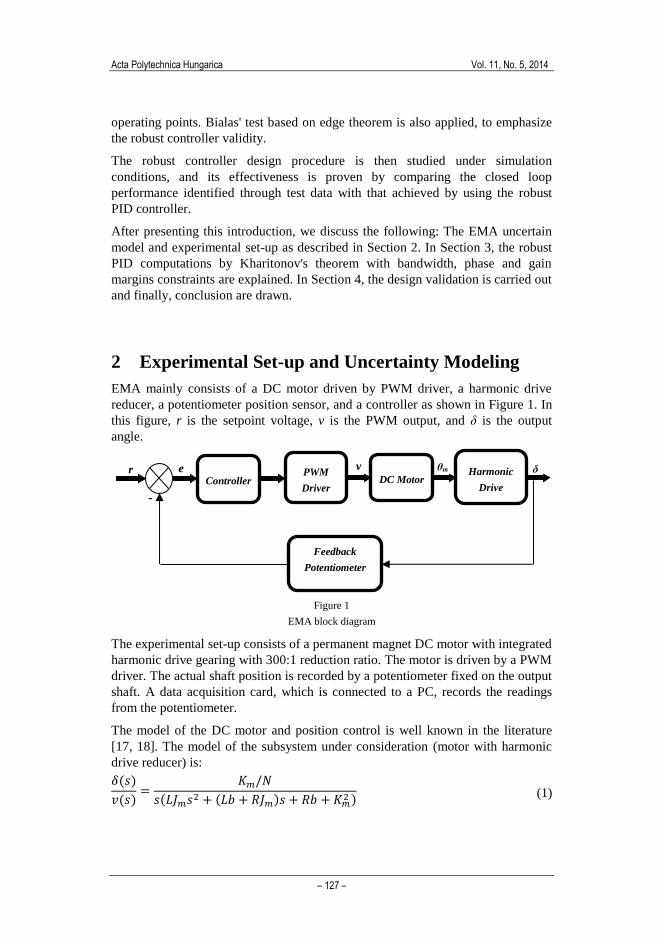
EMA mainly consists of a DC motor driven by PWM driver, a harmonic drive
reducer, a potentiometer position sensor, and a controller as shown in Figure 1. In
this figure, r is the setpoint voltage, v is the PWM output, and δ is the output
angle.
Figure 1
EMA block diagram
The experimental set-up consists of a permanent magnet DC motor with integrated
harmonic drive gearing with 300:1 reduction ratio. The motor is driven by a PWM
driver. The actual shaft position is recorded by a potentiometer fixed on the output
shaft. A data acquisition card, which is connected to a PC, records the readings
from the potentiometer.
The model of the DC motor and position control is well known in the literature
[17, 18]. The model of the subsystem under consideration (motor with harmonic
drive reducer) is:
(1)
r e
-
ᵟ PWM
Driver DC Motor
Harmonic
Drive
θm
Feedback
Potentiometer
v
Controller
R. Salloum et al. Robust PID Controller Design for a Real Electromechanical Actuator
– 128 –
where Km (N.m/A) is the motor's torque constant, L (H) and R (Ohm) are the
inductance and resistance of motor control coil respectively, b (N.m/rad/sec) is the
viscous damping coefficient, N is the harmonic drive gear ratio, and Jm (Kg.m2) is
the rotor's moment of inertia.
Hence, considering that the change of armature current in time is negligible, we
can use engineering judgment to neglect L. In addition, the viscous damping can
be neglected. So, the EMA model can be represented as follows:
(2)
Where K is a constant corresponds to the open loop gain, controller, and motor
constants. Kf is the potentiometer coefficient in v/deg, and
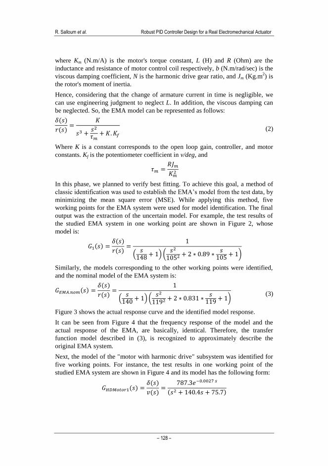
In this phase, we planned to verify best fitting. To achieve this goal, a method of
classic identification was used to establish the EMA’s model from the test data, by
minimizing the mean square error (MSE). While applying this method, five
working points for the EMA system were used for model identification. The final
output was the extraction of the uncertain model. For example, the test results of
the studied EMA system in one working point are shown in Figure 2, whose
model is:
(
) (
)
Similarly, the models corresponding to the other working points were identified,
and the nominal model of the EMA system is:
(
) (
)
(3)
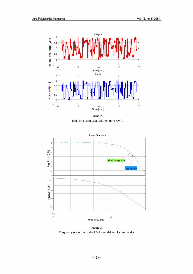
Figure 3 shows the actual response curve and the identified model response.
It can be seen from Figure 4 that the frequency response of the model and the
actual response of the EMA, are basically, identical. Therefore, the transfer
function model described in (3), is recognized to approximately describe the
original EMA system.
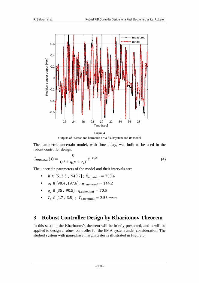
Next, the model of the "motor with harmonic drive" subsystem was identified for
five working points. For instance, the test results in one working point of the
studied EMA system are shown in Figure 4 and its model has the following form:
Acta Polytechnica Hungarica Vol. 11, No. 5, 2014
– 129 –
Figure 2
Input and output data captured from EMA
Figure 3
Frequency responses of the EMA's model and its test results
0 5 10 15 20-1.5
-1
-0.5
0
0.5
1
Time [sec]
Pos
ition
sen
sor
outp
ut [
Vol
ts]
Output
0 5 10 15 20-1.5
-1
-0.5
0
0.5
1
1.5
Time [sec]
Com
man
d [V
olt]
Input
-14
-12
-10
-8
-6
-4
-2
0
2
Mag
nitu
de
(dB
)
10 0 10 1
-180
-135
-90
-45
0
Phase
(d
eg
)
Model response
Test results
Frequency (Hz)
Bode Diagram
R. Salloum et al. Robust PID Controller Design for a Real Electromechanical Actuator
– 130 –
Figure 4
Outputs of "Motor and harmonic drive" subsystem and its model
The parametric uncertain model, with time delay, was built to be used in the
robust controller design.
(4)
The uncertain parameters of the model and their intervals are:
[ ]
[ ]
[ ]
[ ]
3 Robust Controller Design by Kharitonov Theorem
In this section, the Kharitonov's theorem will be briefly presented, and it will be
applied to design a robust controller for the EMA system under consideration. The
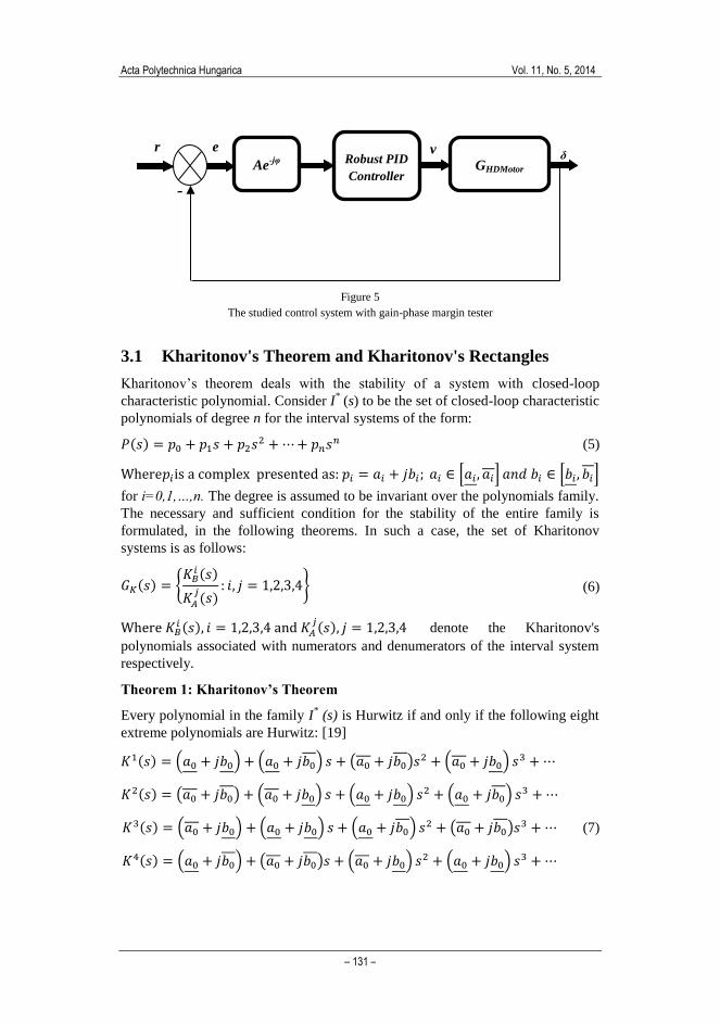
studied system with gain-phase margin tester is illustrated in Figure 5.
22 24 26 28 30 32 34 36 38
-0.6
-0.4
-0.2
0
0.2
0.4
0.6
Time [sec]
Positio
n s
ensor
outp
ut
[Volt]
measured
model
Acta Polytechnica Hungarica Vol. 11, No. 5, 2014
– 131 –
Figure 5
The studied control system with gain-phase margin tester
3.1 Kharitonov's Theorem and Kharitonov's Rectangles
Kharitonov’s theorem deals with the stability of a system with closed-loop
characteristic polynomial. Consider I* (s) to be the set of closed-loop characteristic
polynomials of degree n for the interval systems of the form:
(5)
[ ] [ ]
for i=0,1,…,n. The degree is assumed to be invariant over the polynomials family.
The necessary and sufficient condition for the stability of the entire family is
formulated, in the following theorems. In such a case, the set of Kharitonov
systems is as follows:
{
} (6)
denote the Kharitonov's
polynomials associated with numerators and denumerators of the interval system
respectively.
Theorem 1: Kharitonov’s Theorem
Every polynomial in the family I* (s) is Hurwitz if and only if the following eight
extreme polynomials are Hurwitz: [19]
( ) ( ) ( ) ( )
( ) ( ) ( ) ( )
(7) ( ) ( ) ( ) ( )
( ) ( ) ( ) ( )
r e
-
ᵟ Robust PID
Controller Ae
-jφ GHDMotor
v
R. Salloum et al. Robust PID Controller Design for a Real Electromechanical Actuator
– 132 –
( ) ( ) ( ) ( )
( ) ( ) ( ) ( )
( ) ( ) ( ) ( )
( ) ( ) ( ) ( )
Theorem 2
The closed loop system containing the interval plant G(s) is robustly stable if and
only if each of the Kharitonov systems in is stable. [19]
Definition: Kharitonov Rectangle
Evaluating the four Kharitonov polynomials K1 (s), K
2 (s), K
3 (s), and K
4 (s) at s =
jω0 , the four vertices of Kharitonov's rectangle will be obtained. Therefore, given
an interval polynomial family P (s,q) and a fixed frequency ω = ω0, the value P
(jω0,q) is a rectangle whose vertices are given by Ki (jω0) for i = 1,2,3,4. [19]
Theorem 3: Origin Exclusion for Interval Families
An interval polynomial family has invariant degree and at least one stable
member is robustly stable, if and only if, the origin of the complex plan is
excluded from the Kharitonov's rectangle at all nonnegative frequencies, i.e.
for all frequencies. Practically, it is enough to check the zero
exclusion for all , i.e. for frequencies that are less than the crossover
frequency. [19]
3.2 Controller Design
In this subsection, we design a robust PID controller, which robustly stabilizes the
uncertain system, and guarantees the desired performance of closed loop system.
The required response of the EMA system to be designed, is a deadbeat response
as shown in Table 1.
Table 1
System performance requirements
Parameter Value
Rise time tr < 40 msec
Settling time ts < 60 msec
Steady-state position error 0
Overshoot < 1%
Acta Polytechnica Hungarica Vol. 11, No. 5, 2014
– 133 –
Bandwidth 10 Hz ≤ BW ≤ 40 Hz
Gain margin Gm ≥ 7 dB
Phase margin Pm ≥ 40°
Since the studied system has a time delay and gain-phase margin tester, the
complex Kharitonov system will be used. The closed-loop characteristic
polynomial of EMA system in Figure 5 is:
[ ]
(8)
where Kp, Ki, and Kd are the coefficients of the PID controller. It is clear from (8)
that the polynomial has invariant degree. The coefficients of PID controller Kp, and Ki can be expressed as functions of uncertainties, frequency, and Kd as
follows:
[ ] (9)
By varying the frequency, it is possible to draw the stability boundary in Kp-Ki
plan for certain Kd.
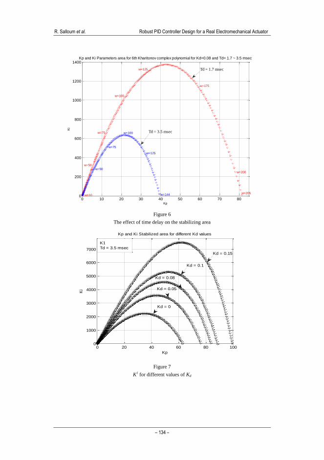
The effect of the time delay Td on the stabilizing region will be verified. The
margins and Kd are assigned to be as follows: A=1, φ = 0° and Kd = 0.08. The
edge polynomial K6(s), which has the smallest stabilizing area, is illustrated in
Figure 6.
The effect of the coefficient Kd is also considered. The larger Kd results in larger
stability region as it is shown in Figure 7 for the first Kharitonov polynomial.
R. Salloum et al. Robust PID Controller Design for a Real Electromechanical Actuator
– 134 –
Figure 6
The effect of time delay on the stabilizing area
Figure 7
K1 for different values of Kd
0 10 20 30 40 50 60 70 800
200
400
600
800
1000
1200
1400
w=10 w=144
w=125
w=205
w=100
w=100
w=175
w=200
w=75
w=75
w=50
w=125
w=50
Kp and Ki Parameters area for 6th Kharitonov complex polynomial for Kd=0.08 and Td= 1.7 ~ 3.5 msec
Kp
Ki
Td = 3.5 msec
Td = 1.7 msec
0 20 40 60 80 1000
1000
2000
3000
4000
5000
6000
7000
Kp and Ki Stabilized area for different Kd values
Kp
Ki
Kd = 0
Kd = 0.05
Kd = 0.08
Kd = 0.1
Kd = 0.15
K1
Td = 3.5 msec

Acta Polytechnica Hungarica Vol. 11, No. 5, 2014
– 135 –
Subsequently, the phase margin constraint is the issue of consideration, Pm ≥ 40°.
In this case, all eight Kharitonov's polynomials are plotted in Figure 8, and the
stabilized area is that restricted under K6 and K
8 polynomials.
Figure 8
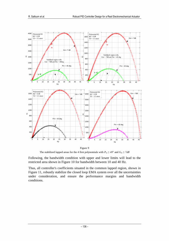
The stabilized lapped area for Pm ≥ 40°
The next step, in addition to the phase margin constraint, the gain margin
constraint will be added Gm ≥ 7 dB. The first four Kharitonov's polynomials are
separately plotted in Figure 9. The lapped region under the two margins curves is
the stabilizing region where the margins constraints are achieved.
0 10 20 30 40 50 60 700
500
1000
1500
2000
2500
3000
3500
Kp
Ki
Kp and Ki Parameters areas extracted from Kharitonov complex polynomials for Kd=0.08 and Pm>=40 deg
K5
K1
K7
K6K2
K3 K4
K8
Stabilized Kp-Ki values
Td = 3.5 msec
Kd = 0.08
R. Salloum et al. Robust PID Controller Design for a Real Electromechanical Actuator
– 136 –
0 5 10 15 20 25 30 35 40 450
500
1000
1500
2000
2500
3000
3500
4000
Kp
Ki
Pm = 40 deg
Gm =7 dB
Stabilized region with:
Gm > 7dB and Pm > 40deg
Polynomial K1
Kd = 0.08
Td = 3.5 msec
w
w
0 5 10 15 20 25 30 35 400
200
400
600
800
1000
1200
1400
1600
Kp
Ki
w
w
Pm = 40 deg
Stabilized region with;
Gm > 7dB and Pm > 40 deg
Gm = 7dB
Polynomial K2
Kd = 0.08
Td = 3.5 msec
0 5 10 15 20 25 30 35 40 450
200
400
600
800
1000
1200
1400
1600
Kp
Ki
Gm = 7dB
Pm = 40 deg
Polynomial K3
Kd = 0.08
Td = 3.5 msec
0 5 10 15 20 25 30 35 40 450
500
1000
1500
2000
2500
3000
3500
4000
Kp
Ki
Gm = 7dB
Pm = 40 deg
Polynomial K4
Kd = 0.08
Td = 3.5 msec
Figure 9
The stabilized lapped areas for the 4 first polynomials with Pm ≥ 40° and Gm ≥ 7dB
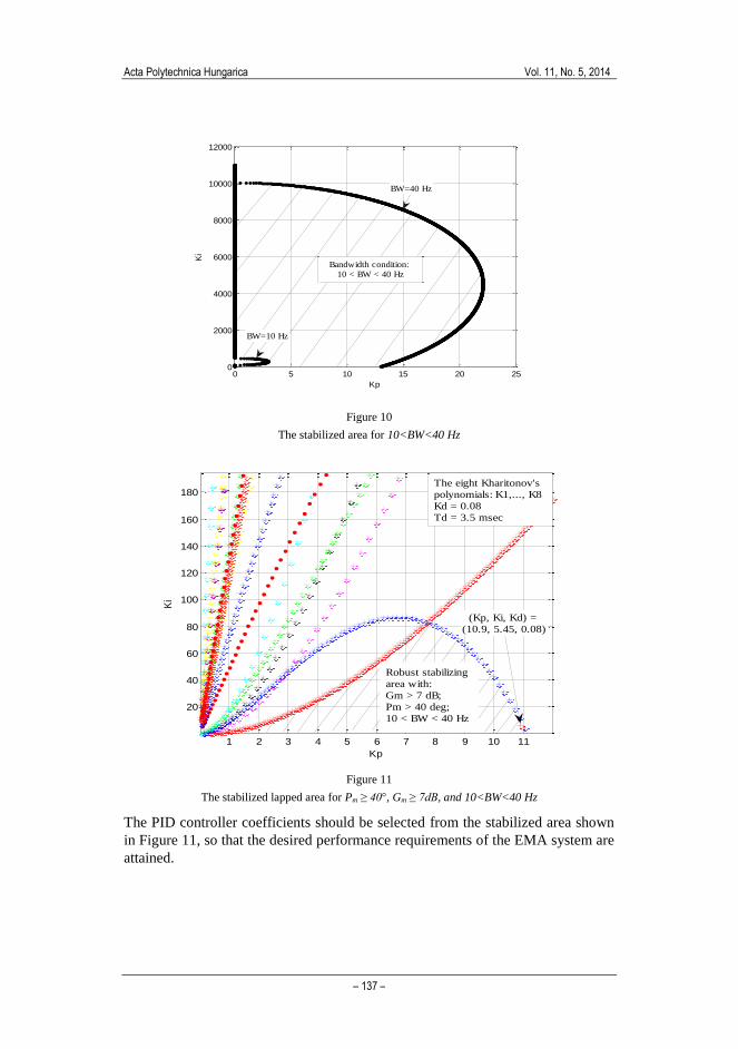
Following, the bandwidth condition with upper and lower limits will lead to the
restricted area shown in Figure 10 for bandwidth between 10 and 40 Hz.
Thus, all controller's coefficients situated in the common lapped region, shown in
Figure 11, robustly stabilize the closed loop EMA system over all the uncertainties
under consideration, and ensure the performance margins and bandwidth
conditions.
Acta Polytechnica Hungarica Vol. 11, No. 5, 2014
– 137 –
Figure 10
The stabilized area for 10<BW<40 Hz
Figure 11
The stabilized lapped area for Pm ≥ 40°, Gm ≥ 7dB, and 10<BW<40 Hz
The PID controller coefficients should be selected from the stabilized area shown
in Figure 11, so that the desired performance requirements of the EMA system are
attained.
0 5 10 15 20 250
2000
4000
6000
8000
10000
12000
Kp
Ki
BW=10 Hz
BW=40 Hz
Bandwidth condition:
10 < BW < 40 Hz
1 2 3 4 5 6 7 8 9 10 11
20
40
60
80
100
120
140
160
180
Kp
Ki
(Kp, Ki, Kd) =
(10.9, 5.45, 0.08)
The eight Kharitonov's
polynomials: K1,..., K8
Kd = 0.08
Td = 3.5 msec
Robust stabilizing
area with:
Gm > 7 dB;
Pm > 40 deg;
10 < BW < 40 Hz

R. Salloum et al. Robust PID Controller Design for a Real Electromechanical Actuator
– 138 –
The selected PID controller is: (Kp, Ki, Kd ) = (10.9, 5.45, 0.08). To affirm the
method validation, the gain and phase margins for the polynomials family with the
designed controller for all the edges uncertainties were extracted and tabulated in
Table 2. It is noted that the constraint of required margins Pm ≥ 40° and Gm ≥ 7dB
is verified.
Table 2
Margins for polynomials family with controller (10.9, 5.45, 0.08)
K q1 q2 Gm (dB) Pm (deg)
949.7 197.6 90.5 16.4 85.5
35 16.4 85.2
90.4 90.5 14.6 59.2
35 14.6 59.1
512.3 197.6 90.5 21.7 87.8
35 21.7 87.3
90.4 90.5 20 69.4
35 20 69
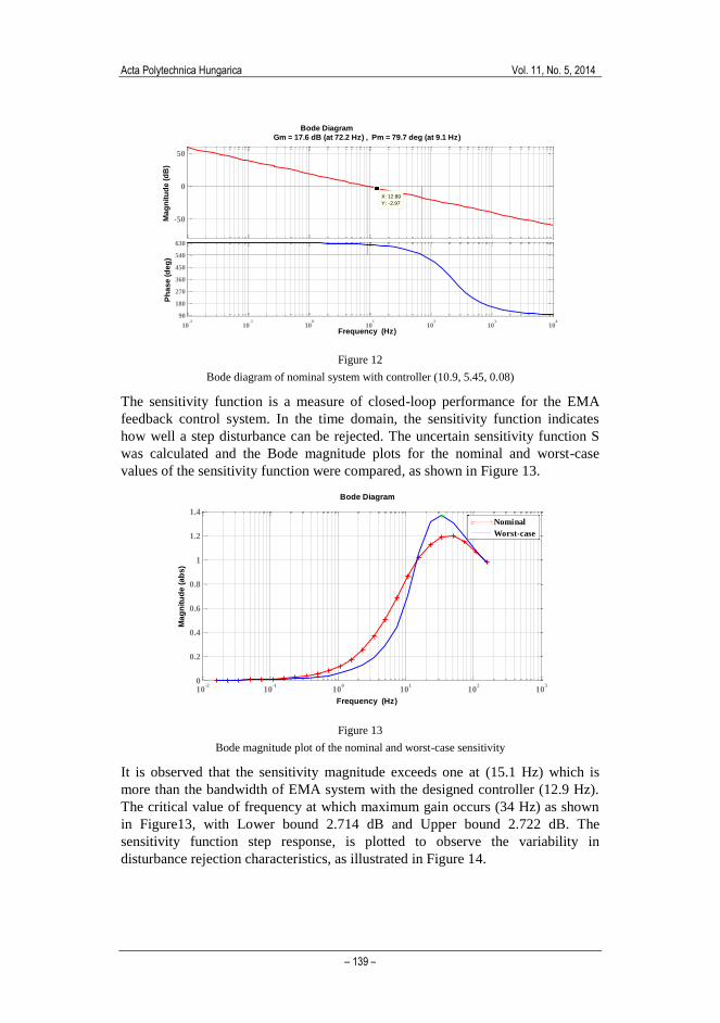
3.3 Stability and Performance Robustness Analysis
Figure 12 is the vivid illustration of the nominal closed-loop system analysis with
maximum time delay, which indicates its high robustness with 17.6 dB gain
margin and 79.7 deg of phase margin with bandwidth 12.9 Hz.
The worst-case analysis (peak-over-frequency type) shows a degradation of the
gain and phase margins to a mere 10 dB and 54.9 deg, which takes place at
frequency 24.5 Hz. However, the margins are still acceptable compared to the
system's requirements. In addition, the frequency at which the worst-case takes
place (24.5 Hz) is somewhat larger than the system's bandwidth.
Acta Polytechnica Hungarica Vol. 11, No. 5, 2014
– 139 –
Figure 12
Bode diagram of nominal system with controller (10.9, 5.45, 0.08)
The sensitivity function is a measure of closed-loop performance for the EMA
feedback control system. In the time domain, the sensitivity function indicates
how well a step disturbance can be rejected. The uncertain sensitivity function S
was calculated and the Bode magnitude plots for the nominal and worst-case
values of the sensitivity function were compared, as shown in Figure 13.
Figure 13
Bode magnitude plot of the nominal and worst-case sensitivity
It is observed that the sensitivity magnitude exceeds one at (15.1 Hz) which is
more than the bandwidth of EMA system with the designed controller (12.9 Hz).
The critical value of frequency at which maximum gain occurs (34 Hz) as shown
in Figure13, with Lower bound 2.714 dB and Upper bound 2.722 dB. The
sensitivity function step response, is plotted to observe the variability in
disturbance rejection characteristics, as illustrated in Figure 14.
10-2
10-1
100
101
102
103
104
90
180
270
360
450
540
630
Ph
as
e (
de
g)
Bode Diagram
Gm = 17.6 dB (at 72.2 Hz) , Pm = 79.7 deg (at 9.1 Hz)
Frequency (Hz)
-50
0
50
X: 12.89
Y: -2.97
Ma
gn
itu
de
(d
B)
10-2
10-1
100
101
102
103
0
0.2
0.4
0.6
0.8
1
1.2
1.4
Ma
gn
itu
de
(a
bs
)
Bode Diagram
Frequency (Hz)
Nominal
Worst-case

R. Salloum et al. Robust PID Controller Design for a Real Electromechanical Actuator
– 140 –
Figure 14
Step response of the nominal and worst-case sensitivity
Since it is enough to test the origin exclusion for (the crossover frequency
which is less than 100 rad/sec in the studied system), the rectangles were plotted
for frequencies ω < 200 rad/sec in Figure 15.
Figure 15
Kharitonov rectangles for the EMA system
As shown in Figure 15, the origin is excluded from the Kharitonov's rectangles,
which affirms that the EMA closed loop system is robustly stable.
0 0.05 0.1 0.15 0.2 0.25 0.3 0.35 0.4-0.2
0
0.2
0.4
0.6
0.8
1
1.2
Disturbance Rejection
Time (sec)
Am
plitu
de
Nominal
Worst-case
-10 -8 -6 -4 -2 0 2
x 106
-5
-4
-3
-2
-1
0
1x 10
6
Real
Imag
inar
y
Kharitononv rectangles for frequency 0 to 200 rad/sec
=10 rad/sec
=50=100
=75
=125
=150
=175
=200 rad/sec

Acta Polytechnica Hungarica Vol. 11, No. 5, 2014
– 141 –
4 Robust Controller Validation
The EMA system, with the new robust controller, will be validated by Bials's test
and by comparing its performance with the original EMA performance.
4.1 Validation by Bialas' Test
Suppose that the polynomials p1 and p2 are strictly Hurwitz with their leading
coefficient nonnegative and the remaining coefficients positive. Let P1 and P2 be
their Hurwitz matrices, and define the matrix:
(10)
Then each of polynomials
[ ] (11)
is strictly Hurwitz iff the real eigenvalues of W all are strictly negative.
Remark: the Hurwitz matrix Q, for the polynomial q(s), is defined as follows
[
]
The designed controller by Kharitonov's theorem should be submitted to the
Bialas' test at its 12 exposed edges.
For the first exposed edge: the two polynomials after numerical substitution are
Which are both Hurwitz . The Hurwiz matrices of these two polynomials are:
[
], [
]
The eigenvalues of are -1, -0.9903, and -1. They are all real and
negative. Hence, by Bials' test, the EMA system is stable on the first edge.
Similarly, the other 11 were checked and the eigenvalues of Wi for i =2… 12 are
all real negative. Another example, the eigenvalues of are -
0.5394, -0.5410, and -0.8718. So, by the edge theorem, the system is robustly
stable for the uncertainties under consideration.

R. Salloum et al. Robust PID Controller Design for a Real Electromechanical Actuator
– 142 –
4.2 Performance Validation
Finally, the step responses of the EMA system with the designed robust controller
and the identified original one were plotted (as illustrated in Figure 16).
Figure 16
Step responses for EMA systems
The main characteristics of the EMA systems are shown in Table 3. The new
designed EMA system, in addition to its robustness to parametric uncertainties
and margins achievement, has no overshoot. In addition, in spite of small
degradation in rise and settling times, they are still within the acceptable ranges.
Table 3
Characteristics of original and robust EMA systems
Model tr (0 ~90%)
(msec)
ts
(msec)
tp
(msec)
Overshoot
(%)
Identified original EMA 25 46 39.5 2.6
Robust EMA 30 48 -- 0
A low pass filter (LPF) is added to the derivative path of the PID controller in
order to pass only low frequency gain and attenuate the high frequency one.
0 50 100 150 200 2500
0.2
0.4
0.6
0.8
1
1.2
1.4
Time [msec]
Positio
n s
ensor
outp
ut
[Volt]
Step response
Command
Identified EMA system
Robust EMA system
Acta Polytechnica Hungarica Vol. 11, No. 5, 2014
– 143 –
To attain the last results, the EMA system with the designed robust controller
secures the robust stability over the uncertainties intervals and attains the required
margins (Pm ≥ 40°, Gm ≥ 7dB) with an acceptable bandwidth. In time domain, it
has no overshoots and no steady-state errors. Therefore, all the required
specifications shown in Table 1 are accomplished.
Conclusions
A novel approach was proposed, to graphically design a robust PID controller, for
a parametric uncertain system with time delay constrained with gain and phase
margins conditions. It was then applied to an EMA system, the designed controller
ensured robust stability, while shaping the performance in a desired fashion.
Finally, in order to validate its practicality, the robust EMA system was compared
with the identified EMA system. In addition, to its robustness, the robust EMA
system proved better dynamic characteristics than the original.
References
[1] C. Gerada, and K. J. Bradley: Integrated PM Machine Design for an
Aircraft EMA, IEEE Transactions on Industrial Electronics, Vol. 55, No. 9,
2008, pp. 3300-3306
[2] D. Howe: Magnetic Actuators, Sensors and Actuators, Vol. 81, 2000, pp.
268-274
[3] J. Liscouët, J.-C. Maré, and M. Budinger: An Integrated Methodology for
the Preliminary Design of Highly Reliable Electromechanical Actuators:
Search for Architecture Solutions, Aerospace Science and Technology,
Vol. 22, 2012, pp. 9-18
[4] E. N. Gonçalves, R. M. Palhares, and R. H. C. Takahashi: H2/H∞ Robust
PID Synthesis for Uncertain Systems, Proceedings of the 45th
IEEE
conference on Decision & Control, San Diego, CA, USA, December 13-15,
2006, pp. 4375-4380
[5] T. Yamamoto, T. Ueda, H. Shimegi, T. Sugie, S. Tujio, and T. Ono: A
Design Method of Robust Controller and Its Application to Positioning
Servo, JSME International Journal, Series III, Vol. 33, No. 4, 1990, pp.
649-654
[6] H. Lu, Y. Li, and C. Zhu: Robust Synthesized Control of Electromechanical
Actuator for Thrust Vector System in Spacecraft, J. Computers and
Mathematics with Applications, Vol. 64, Issue 5, 2012, pp. 699-708
[7] S. E. Lyshevski, R. D. Colgren, and V. A. Skormin: High Performance
Electromechanical Direct-Drive Actuators for Flight Vehicles, Proceedings
of the American Control Conference, Arlington, VA, June 25-27, 2001, pp.
1345-1350
R. Salloum et al. Robust PID Controller Design for a Real Electromechanical Actuator
– 144 –
[8] S. E. Lyshevski: Electromechanical Flight Actuators for Advanced Flight
Vehicles, IEEE Transactions on Aerospace and Electronic Systems Journal,
Vol. 35, No. 2, 1999, pp. 511-518
[9] M. Ristanović, Ž. Ćojbašić, and D. Lazić: Intelligent Control of DC Motor
Driven Electromechanical Fin Actuator, J. Control Engineering Practice,
Vol. 20, 2012, pp. 610-617
[10] C. Yoo, Y. Lee, and S. Lee: A Robust Controller for an Electro-Mechanical
Fin Actuator, Proceeding of the American Control Conference, Boston,
Massachusetts, June 30-July 2, 2004, pp. 4010-4015
[11] J. Dawes, L. Ng, R. Dorf, and C. Tam: Design of Deadbeat Robust
Systems, Glasgow, UK, 1994, pp. 1597-1598
[12] R. Toscano: A Simple Robust PI/PID Controller Design via Numerical
Optimization Approach, J. of Process Control, Vol. 15, 2005, pp. 81-88
[13] D. Valério, J. Costa: Tuning of Fractional Controllers Minimising H2 and
H∞ Norms, Acta Polytechnica Hungarica, Vol. 3, No. 4, 2006, pp. 55-70
[14] R. Bréda, T. Lazar, R. Andoga, and L. Madarász: Robust Controller in the
Structure of Lateral Control of Maneuvering Aircraft, Acta Polytechnica
Hungarica, Vol. 10, No. 5, 2013, pp. 101-124
[15] N. Tan: Computation of Stabilizing PI-PD Controllers, International
Journal of Control, Automation, and Systems, 7(2), 2009, pp. 175-184
[16] Y. J. Huang and Y. J. Wang: Robust PID Tuning Strategy for Uncertain
Plants Based on the Kharitonov Theorem, ISA Transactions, Vol. 39, 2000,
pp. 419-431
[17] P. C. Krause, O. Wasynczuk, and S. D. Sundhoff: Analysis of Electric
Machinery and Drive Systems, IEEE press, 2002
[18] K.-K. Shyu, and Y.-Y. Lee: Identification of Electro-Mechanical Actuators
within Limited Stroke, Journal of Vibration and Control, Vol. 16(12), 2010,
pp. 1737-1761
[19] S. P. Bhattacharyya, H. Chapellat, and L. H. Keel: Robust Control: The
Parametric Approach, Prentice Hall, 1995