robust performance hypothesis testing with the …robust performance hypothesis testing with the...
TRANSCRIPT
Institute for Empirical Research in Economics University of Zurich
Working Paper Series
ISSN 1424-0459
Working Paper No. 320
Robust Performance Hypothesis Testing with the
Sharpe Ratio
Oliver Ledoit and Michael Wolf
January 2008

Robust Performance Hypothesis Testing with the Sharpe Ratio
Oliver Ledoit∗
Equity Proprietary Trading
Credit Suisse
London E14 4QJ, U.K.
E-mail: [email protected]
Michael Wolf†
Institute for Empirical Research in Economics
University of Zurich
CH-8006 Zurich, Switzerland
E-mail: [email protected]
January 2008
Abstract
Applied researchers often test for the difference of the Sharpe ratios of two investment
strategies. A very popular tool to this end is the test of Jobson and Korkie (1981), which
has been corrected by Memmel (2003). Unfortunately, this test is not valid when returns
have tails heavier than the normal distribution or are of time series nature. Instead, we
propose the use of robust inference methods. In particular, we suggest to construct a
studentized time series bootstrap confidence interval for the difference of the Sharpe ratios
and to declare the two ratios different if zero is not contained in the obtained interval.
This approach has the advantage that one can simply resample from the observed data as
opposed to some null-restricted data. A simulation study demonstrates the improved finite
sample performance compared to existing methods. In addition, two applications to real
data are provided.
KEY WORDS: Bootstrap, HAC inference, Sharpe ratio.
JEL CLASSIFICATION NOS: C12, C14, C22.
ACKNOWLEDGMENT: We are grateful for two helpful reports from anonymous referees
which have led to an improved presentation of the paper.
∗The views expressed herein are those of the author and do not necessarily reflect or represent those of Credit
Suisse.†The research has been supported by the University Research Priority Program “Finance and Financial
Markets”, University of Zurich, and by the Spanish Ministry of Science and Technology and FEDER, grant
MTM2006-05650.
1
1 Introduction
Many applications of financial performance analysis are concerned with the comparison of the
Sharpe ratios of two investment strategies (such as stocks, portfolios, mutual funds, hedge
funds, or technical trading rules). Since the true quantities are not observable, the Sharpe
ratios have to be estimated from historical return data and the comparison has to be based on
statistical inference, such as hypothesis tests or confidence intervals.
It appears that the status quo in the applied literature is the test of Jobson and Korkie
(1981) and its corrected version by Memmel (2003); for example, see DeMiguel et al. (2008),
DeMiguel and Nogales (2007), and Gasbarro et al. (2007), among others. Unfortunately, this
test is not valid when returns have tails heavier than the normal distribution or are of time
series nature. The former is a quite common, and by now well-known, property of financial
returns. As far as the latter is concerned, serial correlation of the actual returns is, arguably,
only a minor concern for stocks and mutual funds, but it is certainly relevant to hedge funds;
for example, see Brooks and Kat (2002) and Malkiel and Saha (2005). However, even stocks
and mutual funds often exhibit correlation of the squared returns, that is, volatility clustering;
for example, see Campbell et al. (1997, Chapter 12) and Alexander (2001, Chapter 4).
In this paper, we discuss inference methods that are more generally valid. One possibility
is to compute a HAC standard error1 for the difference of the estimated Sharpe ratios by
the methods of Andrews (1991) and Andrews and Monahan (1992), say. Such an approach
works asymptotically but does not always have satisfactory properties in finite samples. As an
improved alternative, we suggest a studentized time series bootstrap.
It has been argued that for certain applications the Sharpe ratio is not the most appropriate
performance measure; e.g., when the returns are far from normally distributed or autocorre-
lated (which happens for many hedge funds) or during bear markets. On the other hand, there
is recent evidence that the Sharpe ratio can result in almost identical fund rankings compared
to alternative performance measures; e.g., see Eling and Schuhmacher (2007). We do not enter
this debate. Instead, we believe that the task of choosing the appropriate performance measure
is up to the finance practitioner, not the statistician. Our aim is to provide a reliable inference
method in case the comparison of two Sharpe ratios is deemed of interest.
2 The Problem
We use the same notation as Jobson and Korkie (1981) and Memmel (2003). There are two
investment strategies i and n whose excess returns over a given benchmark at time t are rti and
rtn, respectively. Typically, the benchmark is the riskfree rate but it could also be something
1In this paper, a standard error of an estimator denotes an estimate of the true standard deviation of the
estimator.
2
else, such as a stock index.2 A total of T return pairs (r1i, r1n)′, . . . , (rT i, rTn)′ are observed.
It is assumed that these observations constitute a strictly stationary time series so that, in
particular, the bivariate return distribution does not change over time. This distribution has
mean vector µ and covariance matrix Σ given by
µ =
(µi
µn
)and Σ =
(σ2
i σin
σin σ2n
).
The usual sample means and sample variances of the observed returns are denoted by µi, µn
and σ2i , σ
2n, respectively. The difference between the two Sharpe ratios is given by
∆ = Shi − Shn =µi
σi− µn
σn
and its estimator is
∆ = Shi − Shn =µi
σi− µn
σn.
Furthermore, let u = (µi, µn, σ2i , σ
2n)′ and u = (µi, µn, σ2
i , σ2n)′. Memmel (2003) computes a
standard error for ∆ based on the relation
√T (u − u)
d→ N(0;Ω) ,
whered→ denotes convergence in distribution, and an application of the delta method. However,
just like Jobson and Korkie (1981), he uses a formula for Ω that crucially relies on i.i.d. return
data from a bivariate normal distribution, namely he assumes
Ω =
σ2i σin 0 0
σin σ2n 0 0
0 0 2σ4i 2σ2
in
0 0 2σ2in 2σ4
n
.
This formula is no longer valid if the distribution is non-normal or if the observations are
correlated over time. To give just two examples, consider data that are i.i.d. but not necessarily
normal. First, the entry in the lower right corner of Ω is given by E[(r1n−µn)4]−σ4n instead of
by 2σ4n. Second, the asymptotic covariance between µn and σ2
n, say, is in general not equal to
zero.3 To give another example, consider data from a stationary time series. Then the entry
in the upper left corner is given by σ2i + 2
∑∞t=1 Cov(r1i, r(1+t)i) instead of by simply σ2
i .
3 Solutions
We find it somewhat more convenient to work with the uncentered second moments. So let
γi = E(r21i) and γn = E(r2
1n). Their sample counterparts are denoted by γi and γn, respectively.
2Strictly speaking, when the benchmark is a stock index, say, rather than the riskfree rate, one should speak
of the Information ratio rather than the Sharpe ratio.3For example, consider data from a Poisson distribution, in which case µ and σ2 estimate the same parameter.
3

Furthermore, let v = (µi, µn, γi, γn)′ and v = (µi, µn, γi, γn)′. This allows us to write
∆ = f(v) and ∆ = f(v) (1)
with
f(a, b, c, d) =a√
c − a2− b√
d − b2. (2)
We assume that √T (v − v)
d→ N(0;Ψ) , (3)
where Ψ is an unknown symmetric positive semi-definite matrix. This relation holds under mild
regularity conditions. For example, when the data are assumed i.i.d., it is sufficient to have
both E(r41i) and E(r4
1n) finite. In the time series case it is sufficient to have finite 4+δ moments,
where δ is some small positive constant, together with an appropriate mixing condition; for
example, see Andrews (1991). The delta method then implies
√T (∆ − ∆)
d→ N(0;∇′f(v)Ψ∇f(v)) (4)
with
∇′f(a, b, c, d) =
(c
(c − a2)1.5, − d
(d − b2)1.5, −1
2
a
(c − a2)1.5,
1
2
b
(d − b2)1.5
).
Now, if a consistent estimator Ψ of Ψ is available, then a standard error for ∆ is given by
s(∆) =
√∇′f(v)Ψ∇f(v)
T. (5)
3.1 HAC Inference
As is well-known, the limiting covariance matrix in (3) is given by
Ψ = limT→∞
1
T
T∑
s=1
T∑
t=1
E[ysy′t], with y′t = (rti − µ1, rtn − µn, r2
ti − γi, r2tn − γn) .
By change of variables, the limit can be alternatively expressed as
Ψ = limT→∞
ΨT , with ΨT =
T−1∑
j=−T+1
ΓT (j), where
ΓT (j) =
1T
∑Tt=j+1 E[yty
′t−j] for j ≥ 0
1T
∑Tt=−j+1 E[yt+jy
′t] for j < 0
.
The standard method to come up with a consistent estimator Ψ = ΨT is to use het-
eroskedasticity and autocorrelation robust (HAC) kernel estimation; for example, see Andrews
(1991) and Andrews and Monahan (1992). In practice this involves choosing a real-valued ker-
nel function k(·) and a bandwidth ST . The kernel k(·) typically satisfies the three conditions
4
k(0) = 1, k(·) is continuous at 0, and limx→±∞ k(x) = 0. The kernel estimate for Ψ is then
given by
Ψ = ΨT =T
T − 4
T−1∑
j=−T+1
k
(j
ST
)ΓT (j), where
ΓT (j) =
1T
∑Tt=j+1 yty
′t−j for j ≥ 0
1T
∑Tt=−j+1 yt+j y
′t for j < 0
, with y′t = (rti − µ1, rtn − µn, r2ti − γi, r
2tn − γn) .
The factor T/(T − 4) is a small-sample degrees of freedom adjustment that is introduced to
offset the effect of the estimation of the 4-vector v in the computation of the ΓT (j), that is,
the use of the yt rather than the yt.
An important feature of a kernel k(·) is its characteristic exponent 1 ≤ q ≤ ∞, determined
by the smoothness of the kernel at the origin. Note that the bigger q, the smaller is the
asymptotic bias of a kernel variance estimator; on the other hand, only kernels with q ≤ 2
yield estimates that are guaranteed to be positive semi-definite in finite samples. Most of
the commonly used kernels have q = 2, such as the Parzen, Tukey-Hanning, and Quadratic-
Spectral (QS) kernels, but exceptions do exist. For example, the Bartlett kernel has q = 1
and the Truncated kernel has q = ∞. For a broader discussion on this issue, see see Andrews
(1991) again.
Once a particular kernel k(·) has been chosen for application, one must pick the band-
width ST . Several automatic methods, based on various asymptotic optimality criteria, are
available to this end; for example, see Andrews (1991) and Newey and West (1994).
Finally, given the kernel estimator Ψ, the standard error s(∆) is obtained as in (5) and
then combined with the asymptotic normality (4) to make HAC inference as follows.
A two-sided p-value for the null hypothesis H0: ∆ = 0 is given by
p = 2Φ
(− |∆|
s(∆)
)
where Φ(·) denotes the c.d.f. of the standard normal distribution. Alternatively, a 1 − α
confidence interval for ∆ is given by
∆ ± z1−α/2 s(∆)
where zλ denotes the λ quantile of the standard normal distribution, that is, Φ(zλ) = λ.
It is, however, well known that such HAC inference is often liberal when samples sizes are
small to moderate. This means hypothesis tests tend to reject a true null hypothesis too often
compared to the nominal significance level and confidence intervals tend to undercover; for
example, see Andrews (1991), Andrews and Monahan (1992), and Romano and Wolf (2006).
Remark 3.1 Lo (2002) discusses inference for a single Sharpe ratio. The method he presents
in the section titled “IID Returns” corresponds to Jobson and Korkie (1981) and Memmel
5

(2003), since it actually assumes i.i.d. normal data. The method he presents in the section
titled “Non-IID Returns” corresponds to the HAC inference of this subsection.
Opdyke (2007) discusses both inference for a single Sharpe ratio and for the difference of
two Sharpe ratios. He first considers the case of general i.i.d. data (i.e., not necessarily normal)
and corrects the formulae for the limiting variances of Lo (2002, Section “IID Returns”) and
of Memmel (2003), respectively, which assume normality. He also considers the case of general
stationary data (i.e., time series). However, his formulae for the time series case are incorrect,
since they are equivalent to the formulae for the i.i.d. case. For example, the limiting variance
in (6), for the case of general stationary data, is equivalent to the limiting variance in (3), for
general i.i.d. data.
3.2 Bootstrap Inference
There is an extensive literature demonstrating the improved inference accuracy of the stu-
dentized bootstrap over ‘standard’ inference based on asymptotic normality; see Hall (1992)
for i.i.d. data and Lahiri (2003) for time series data. Very general results are available for
parameters of interests which are smooth functions of means. Our parameter of interest, ∆,
fits this bill; see (1) and (2).
Arguably, the regularity conditions used by Lahiri (2003, Section 6.5) in the time series case
are rather strong (and too strong for most financial applications); for example, they assume
35+δ finite moments (where δ is some small number) and certain restrictions on the dependence
structure.4 However, it should be pointed out that these conditions are sufficient only to prove
the very complex underlying mathematics and not necessary. Even when these conditions do
not hold, the studentized bootstrap typically continues to outperform ‘standard’ inference; e.g.,
see Section 4. To avoid any confusion, it should also be pointed that these strong regularity
conditions are only needed to prove the superiority of the studentized bootstrap. In terms
of first-order consistency it does not really need stronger sufficient conditions than ‘standard’
inference.
We propose to test H0: ∆ = 0 by inverting a bootstrap confidence interval. That is, one
constructs a two-sided bootstrap confidence interval with nominal level 1 − α for ∆. If this
interval does not contain zero, then H0 is rejected at nominal level α. The advantage of this
‘indirect’ approach is that one can simply resample from the observed data. If one wanted to
carry out a ‘direct’ bootstrap test, one would have to resample from a probability distribution
that satisfied the constraint of the null hypothesis, that is, from some modified data where the
two empirical Sharpe ratios were exactly equal; e.g., see Politis et al. (1999, Section 1.8).
In particular, we propose to construct a symmetric studentized bootstrap confidence inter-
val. To this end the two-sided distribution function of the studentized statistic is approximated
4The conditions are too lengthy to be reproduced here.
6

via the bootstrap as follows:
L(|∆ − ∆|
s(∆)
)≈ L
(|∆∗ − ∆|
s(∆∗)
). (6)
In this notation, ∆ is true difference between the Sharpe ratios, ∆ is the estimated difference
computed from the original data, s(∆) is a standard error for ∆ (also computed from the
original data), ∆∗ is the estimated difference computed from bootstrap data, and s(∆∗) is
a standard error for ∆∗ (also computed from bootstrap data). Finally, L(X) denotes the
distribution of the random variable X.
Letting z∗|·|,λ be a λ quantile of L(|∆∗ − ∆|/s(∆∗)), a bootstrap 1 − α confidence interval
for ∆ is then given by
∆ ± z∗|·|,1−α s(∆) . (7)
The point is that when data are heavy-tailed or of time series nature, then z∗|·|,1−α will typically
be somewhat larger than z1−α/2 for small to moderate samples, resulting in more conservative
inference compared to the HAC methods of the previous subsection.
We are left to specify (i) how the bootstrap data are to be generated and (ii) how the
standard errors s(∆) and s(∆∗) are to be computed. For this, it is useful to distinguish
between i.i.d. data and time series data. The first case, i.i.d. data, is included mainly for
completeness of the exposition. It is well-known that financial returns are generally not i.i.d..
Even when the autocorrelation of the returns is negligible (which often happens with the stock
and mutual fund returns), there usually exists autocorrelation of the squared returns, that is,
volatility clustering. We therefore recommend to always use the bootstrap method for time
series data in practice.
3.2.1 I.I.D. Data
To generate bootstrap data, one simply uses Efron’s (1979) bootstrap, resampling individual
pairs from the observed pairs (rti, rtn)′, t = 1, . . . , T , with replacement. The standard error
s(∆) is computed as in (5). Since the data are i.i.d., one takes for Ψ here simply the sample
covariance matrix of the vectors (rti, rtn, r2ti, r
2tn)′, t = 1, . . . , T . The standard error s(∆∗) is
computed in exactly the same fashion but from the bootstrap data instead of the original data.
To be more specific, denote the tth return pair of the bootstrap sample by (r∗ti, r∗tn)′. Then
one takes for Ψ∗ the sample covariance matrix of the vectors (r∗ti, r∗tn, r∗ti
2, r∗tn2)′, t = 1, . . . , T .
Furthermore, the estimator of v = (µi, µn, γi, γn)′ based on the bootstrap data is denoted by
v∗ = (µ∗i , µ
∗n, γ∗
i , γ∗n)′. Finally, the bootstrap standard error for ∆∗ is given by
s(∆∗) =
√∇′f(v∗)Ψ∗∇f(v∗)
T. (8)
7

3.2.2 Time Series Data
The application of the studentized bootstrap is somewhat more involved when the data are
of time series nature. To generate bootstrap data, we use the circular block bootstrap of
Politis and Romano (1992), resampling now blocks of pairs from the observed pairs (rti, rtn)′,
t = 1, . . . , T , with replacement.5 These blocks have a fixed size b ≥ 1. The standard error
s(∆) is computed as in (5). The estimator Ψ is obtained via kernel estimation; in particular
we propose the prewhitened QS kernel of Andrews and Monahan (1992).6 The standard
error s(∆∗) is the ‘natural’ standard error computed from the bootstrap data, making use
of the special block dependence structure; see Gotze and Kunsch (1996) for details. To be
more specific, let l = bn/bc, where b·c denotes the integer part. Again, the estimator of
v = (µi, µn, γi, γn)′ based on the bootstrap data is denoted by v∗ = (µ∗i , µ
∗n, γ∗
i , γ∗n)′. Then
define
y∗t = (r∗ti − µ∗i , r
∗tn − µ∗
n, r∗ti2 − γ∗
i , r∗tn2 − γ∗
n)′ t = 1, . . . , T
ζj =1√b
b∑
t=1
y∗(j−1)b+t t = 1, . . . , l
and
Ψ∗ =1
l
l∑
j=1
ζjζ′j .
With this more general definition7 of Ψ∗, the bootstrap standard error for ∆∗ is again given
by formula (8).
An application of the studentized circular block bootstrap requires a choice of the block
size b. To this end, we suggest to use a calibration method, a concept dating back to Loh (1987).
One can think of the actual coverage level 1 − λ of a block bootstrap confidence interval as
a function of the block size b, conditional on the underlying probability mechanism P which
generated the bivariate time series of returns, the nominal confidence level 1 − α, and the
sample size T . The idea is now to adjust the ‘input’ b in order to obtain the actual coverage
level close to the desired one. Hence, one can consider the block size calibration function
g : b → 1 − λ. If g(·) were known, one could construct an ‘optimal’ confidence interval by
finding b that minimizes |g(b) − (1 − α)| and then use b as the block size of the time series
bootstrap; note that |g(b) − (1 − α)| = 0 may not always have a solution.
Of course, the function g(·) depends on the underlying probability mechanism P and is
therefore unknown. We now propose a bootstrap method to estimate it. The idea is that
5The motivation for using the circular block bootstrap instead of the moving blocks bootstrap of Kunsch
(1989) is to avoid the ‘edge effects’ of the latter; see Romano and Wolf (2006, Section 4).6We have found that the prewhitened Parzen kernel, which is defined analogously, yields very similar perfor-
mance.7Note that for the special case b = 1, this definition results in the sample covariance matrix of the bootstrap
data (r∗ti, r∗tn, r∗ti
2, r∗tn
2)′, t = 1, . . . T , used for i.i.d. data.
8

in principle we could simulate g(·) if P were known by generating data of size T according
to P and by computing confidence intervals for ∆ for a number of different block sizes b. This
process is then repeated many times and for a given b, one estimates g(b) as the fraction of the
corresponding intervals that contain the true parameter. The method we propose is identical
except that P is replaced by an estimate P and that the true parameter ∆ is replaced by the
‘pseudo’ parameter ∆.
Algorithm 3.1 (Choice of the Block Size)
1. Fit a semi-parametric model P to the observed data (r1i, r1n)′, . . . , (rT i, rTn)′.
2. Fix a selection of reasonable block sizes b.
3. Generate K pseudo sequences (r∗1i, r∗1n)′k . . . , (r∗T i, r
∗Tn)′k, k = 1, . . . ,K, according to P .
For each sequence, k = 1, . . . ,K, and for each b, compute a confidence interval CIk,b with
nominal level 1 − α for ∆.
4. Compute g(b) = #∆ ∈ CIk,b/K.
5. Find the value b that minimizes |g(b) − (1 − α)|.
Of course, the question remains which semi-parametric model to fit to the observed return
data. When using monthly data, we recommend to simply use a VAR model in conjunction
with time series bootstrapping the residuals.8 If the data are sampled at finer intervals, such
as daily data, one might want to use a bivariate GARCH model instead.
Next, one might ask what is a selection of reasonable block sizes? The answer is any
selection that contains a b with g(b) very close to 1 − α. If nothing else, this can always be
determined by trial and error. In our experience, g(·) is typically monotonically decreasing in b.
So if one starts with blow = 1 and a bup ‘sufficiently’ large, one is left to specify some suitable
grid between those two values. In our experience, again, for a sample size of T = 120, the
choices blow = 1 and bup = 10 usually suffice. In that case the final selection 1, 2, 4, 6, 8, 10should be fine, as g(·) does not tend to decrease very fast in b.
Finally, how large should K be chosen in application to real data? The answer is as large as
possible, given the computational resources. K = 5, 000 will certainly suffice for all practical
purposes, while K = 1, 000 should be the lower limit.
Remark 3.2 As outlined above, a two-sided test for H0: ∆ = 0 at significance level α can
be carried out by constructing a bootstrap confidence interval with confidence level 1 − α.
The test rejects if zero is not contained in the interval. At times, it might be more desirable
8At this point we opt for the stationary bootstrap of Politis and Romano (1994), since it is quite insensitive
to the choice of the average block size. The motivation for time series bootstrapping the residuals is to account
for some possible ‘left over’ non-linear dependence not captured by the linear VAR model.
9

to obtain a p-value. In principle, such a p-value could be computed by ‘trial and error’ as
the smallest α for which the corresponding 1 − α confidence interval does not contain zero.
However, such a procedure is rather cumbersome. Fortunately, there exists a shortcut that
allows for an equivalent ‘direct’ computation of such a p-value. Denote the original studentized
test statistic by d, that is,
d =|∆|
s(∆)
and denote the centered studentized statistic computed from the mth bootstrap sample by
d∗,m, m = 1, . . . ,M , that is,
d∗,m =|∆∗,m − ∆|
s(∆∗,m),
where M is the number of bootstrap resamples. Then the p-value is computed as
PV =#d∗,m ≥ d + 1
M + 1. (9)
Remark 3.3 As far as we know, there have been two previous proposals to use bootstrap
inference for Sharpe ratios, but both are somewhat limited.
Vinod and Morey (1999) discuss inference for the difference of two Sharpe ratios. However,
they only employ Efron’s (1979) i.i.d. bootstrap, so their approach would not work for time
series data. Moreover, the way they studentize in the bootstrap world is incorrect, as they use
a common standard error for all bootstrap statistics. (Instead, one must compute an individual
standard error from each bootstrap data set, as described before.)
Scherer (2004) discusses inference for a single Sharpe ratio, but his approach could be
easily extended to inference for a difference of two Sharpe ratios. Unlike us, he employs a
non-studentized bootstrap for both i.i.d. and time series data. The problem is that a non-
studentized bootstrap does not provide improved inference accuracy compared to ‘standard’
inference based on asymptotic normality; again see Hall (1992) and Lahiri (2003). Scherer
(2004) addresses this problem for i.i.d. data by employing a double bootstrap (which also
provides improved inference accuracy; Hall, 1992), but he does not address it for time series
data. Moreover, his time series bootstrap is of parametric nature, based on an AR(1) model
with i.i.d. errors, and would therefore not be valid in general.
Incidentally, the asymptotically valid approaches detailed in this paper, HAC inference and
the studentized bootstrap, can be easily modified to make inference for a single Sharpe ratio.
The details are straightforward and left to the reader.
4 Simulation Study
The purpose of this section is to shed some light on the finite sample performance of the
various methods via some (necessarily limited) simulations. We compute empirical rejection
10

probabilities under the null, based on 5,000 simulations per scenario. The nominal levels
considered are α = 0.01, 0.5, 0.1. All bootstrap p-values are computed as in (9), employing
M = 499. The sample size is T = 120 always.9
4.1 Competing Methods
The following methods are included in the study:
• (JKM) The test of Jobson and Korkie (1981), using the corrected version of Memmel
(2003).
• (HAC) The HAC test of Subsection 3.1 based on the QS kernel with automatic band-
width selection of Andrews (1991).
• (HACPW ) The HAC test of Subsection 3.1 based on the prewhitened QS kernel with
automatic bandwidth selection of Andrews and Monahan (1992).
• (Boot-IID) The bootstrap method of Subsubsection 3.2.1.
• (Boot-TS) The bootstrap method of Subsubsection 3.2.2. We use Algorithm 3.1 to
pick a data-dependent block size from the input block sizes b ∈ 1, 2, 4, 6, 8, 10. The
semi-parametric model used is a VAR(1) model in conjunction with bootstrapping the
residuals. For the latter we employ the stationary bootstrap of Politis and Romano
(1994) with an average block size of 5.
4.2 Data Generating Processes
In all scenarios, we want the null hypothesis of equal Sharpe ratios to be true. This is easiest
achieved if the two marginal return processes are identical.
It is natural to start with i.i.d. bivariate normal data with equal mean 1 and equal vari-
ance 1. The within-pair correlation is chosen as ρ = 0.5, which seems a reasonable number for
many applications. This DGP is denoted by Normal-IID.
We then relax the strict i.i.d. normal assumption in various dimensions.
First, we keep the i.i.d. assumption but allow for heavy tails. To this end, we use bivariate
t6 data, shifted to have equal mean 1 and standardized to have common variance 1. The
within-pair correlation is ρ = 0.5 again. This DGP is denoted by t6-IID.
Next, we consider an uncorrelated process but with correlations in the squared returns, as
is typical for stock returns. The standard way to model this is via a bivariate GARCH(1,1)
model. In particular, we use the bivariate diagonal-vech model dating back to Bollerslev et al.
(1988). Let rti = rti − µi, rtn = rtn − µn, and denote by Ωt−1 the conditioning information
available at time t − 1. Then the diagonal-vech model is defined by
9Many empirical applications use ten years of monthly data.
11

E(rti|Ωt−1) = 0
E(rtn|Ωt−1) = 0
Cov(rtirtn|Ωt−1) = htin
= cin + ain r(t−1)i r(t−1)n + bin h(t−1)in .
In other words, the conditional (co)variances depend only on their own lags and the lags of
the corresponding (cross)products. We use the following coefficient matrices:
C =
(0.15 0.13
0.13 0.15
)A =
(0.075 0.050
0.050 0.075
)B =
(0.90 0.89
0.90 0.89
)
These matrices are inspired by the bivariate estimation results based on weekly returns on a
broad U.S. market index and a broad U.K. market index.10 However, all three diagonals are
forced to be equal to get identical individual return processes; (2003, Table 2).
The first variant of the GARCH model uses i.i.d. bivariate standard normal innovations
to recursively generate the series rt = (rti, rtn)′. At the end, we add a global mean, that is,
rt = rt + µ, where µ is chosen as µ = (16.5/52, 16.5/52)′ . Again this choice is inspired by
the previously mentioned estimation results, forcing µi = µn to get identical individual return
processes; see Ledoit et al. (2003) (2003, Table 1). This DGP is denoted by Normal-GARCH.
The second variant of the GARCH model uses i.i.d. bivariate t6 innovations instead (stan-
dardized to have common variance equal to 1, and covariance equal to 0).11 Everything else is
equal. This DGP is denoted by t6-GARCH.
Finally, we also consider correlated processes. To this end, we return to the two i.i.d. DGPs
Normal-IID and t6-IID, respectively, but add some mild autocorrelation to the individual return
series via an AR(1) structure with AR coefficient φ = 0.2.12 This then corresponds to a VAR(1)
model with bivariate normal or (standardized) t6 innovations. The resulting two DGPs are
denoted by Normal-VAR and t6-VAR, respectively.
4.3 Results
The results are presented in Table 1 and summarized as follows:
• JKM works well for i.i.d. bivariate normal data but is not robust against fat tails or time
series effects, where it becomes liberal.
10We use estimation results based on weekly returns, since generally there are very few GARCH effects at
monthly or longer return horizons. With weekly data, T = 120 corresponds to a data window of slightly over
two years.11There is ample evidence that the innovations of GARCH processes tend to have tails heavier than the
normal distribution; e.g., see Kuester et al. (2006) and the references therein.12For example, a first-order autocorrelation around 0.2 is quite typical for monthly hedge fund returns.
12
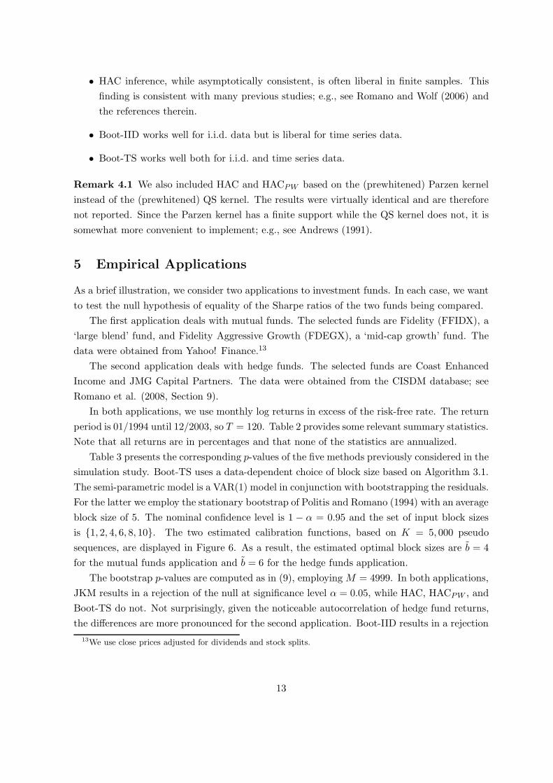
• HAC inference, while asymptotically consistent, is often liberal in finite samples. This
finding is consistent with many previous studies; e.g., see Romano and Wolf (2006) and
the references therein.
• Boot-IID works well for i.i.d. data but is liberal for time series data.
• Boot-TS works well both for i.i.d. and time series data.
Remark 4.1 We also included HAC and HACPW based on the (prewhitened) Parzen kernel
instead of the (prewhitened) QS kernel. The results were virtually identical and are therefore
not reported. Since the Parzen kernel has a finite support while the QS kernel does not, it is
somewhat more convenient to implement; e.g., see Andrews (1991).
5 Empirical Applications
As a brief illustration, we consider two applications to investment funds. In each case, we want
to test the null hypothesis of equality of the Sharpe ratios of the two funds being compared.
The first application deals with mutual funds. The selected funds are Fidelity (FFIDX), a
‘large blend’ fund, and Fidelity Aggressive Growth (FDEGX), a ‘mid-cap growth’ fund. The
data were obtained from Yahoo! Finance.13
The second application deals with hedge funds. The selected funds are Coast Enhanced
Income and JMG Capital Partners. The data were obtained from the CISDM database; see
Romano et al. (2008, Section 9).
In both applications, we use monthly log returns in excess of the risk-free rate. The return
period is 01/1994 until 12/2003, so T = 120. Table 2 provides some relevant summary statistics.
Note that all returns are in percentages and that none of the statistics are annualized.
Table 3 presents the corresponding p-values of the five methods previously considered in the
simulation study. Boot-TS uses a data-dependent choice of block size based on Algorithm 3.1.
The semi-parametric model is a VAR(1) model in conjunction with bootstrapping the residuals.
For the latter we employ the stationary bootstrap of Politis and Romano (1994) with an average
block size of 5. The nominal confidence level is 1 − α = 0.95 and the set of input block sizes
is 1, 2, 4, 6, 8, 10. The two estimated calibration functions, based on K = 5, 000 pseudo
sequences, are displayed in Figure 6. As a result, the estimated optimal block sizes are b = 4
for the mutual funds application and b = 6 for the hedge funds application.
The bootstrap p-values are computed as in (9), employing M = 4999. In both applications,
JKM results in a rejection of the null at significance level α = 0.05, while HAC, HACPW , and
Boot-TS do not. Not surprisingly, given the noticeable autocorrelation of hedge fund returns,
the differences are more pronounced for the second application. Boot-IID results in a rejection
13We use close prices adjusted for dividends and stock splits.
13
for the mutual funds data but not for the hedge fund data. However, as discussed previously,
we recommend to always use Boot-TS with financial return data.
6 Conclusion
Testing for the equality of the Sharpe ratios of two investment strategies is an important tool
for performance analysis. The current status quo method in the applied literature appears to
be the test of Memmel (2003), which is a corrected version of the original proposal of Jobson
and Korkie (1981). Unfortunately, this test is not robust against tails heavier than the normal
distribution and time series characteristics. Since both effects are quite common with financial
returns, the test should not be used.
We have discussed alternative inference methods which are robust. HAC inference uses
kernel estimators to come up with consistent standard errors. The resulting inference works
well with large samples but is often liberal for small to moderate sample sizes. In such appli-
cations, it is preferable to use a studentized time series bootstrap. Arguably, this procedure
is quite complex to implement, but corresponding programming code is freely available at
http://www.iew.uzh.ch/chairs/wolf/team/wolf/publications en.html.
Finally, both the HAC inference and the studentized bootstrap detailed in this paper could
be modified to make inference for (the difference of) various refinements to the Sharpe ratio
recently proposed in the literature—e.g., see Ferruz and Vicente (2005) and Israelsen (2003,
2005)—as well as many other performance measures, such as the Information ratio, Jensen’s
alpha, or the Treynor ratio, to name just a few.
14

References
Alexander, C. (2001). Market Models: A Guide To Financial Data Analysis. John Wiley &
Sons Ltd., Chichester.
Andrews, D. W. K. (1991). Heteroskedasticity and autocorrelation consistent covariance matrix
estimation. Econometrica, 59:817–858.
Andrews, D. W. K. and Monahan, J. C. (1992). An improved heteroskedasticity and autocor-
relation consistent covariance matrix estimator. Econometrica, 60:953–966.
Bollerslev, T., Engle, R. F., and Wooldridge, J. M. (1988). Modelling the coherence in short-
run nominal exchange rates: A multivariate Generalized ARCH model. Review of Economics
and Statistics, 72:498–505.
Brooks, C. and Kat, H. (2002). The statistical properties of hedge fund index returns and
their implications for investors. Journal of Alternative Investments, 5(Fall):26–44.
Campbell, J. Y., Lo, A. W., and MacKinlay, A. C. (1997). The Econometrics of Financial
Markets. Princeton University Press, New Jersey.
DeMiguel, V., Garlappi, L., and Uppal, R. (2008). Optimal versus naive diversification: How
inefficient is the 1/N portfolio strategy? Review of Financial Studies. Forthcoming.
DeMiguel, V. and Nogales, F. J. (2007). Portfolio selection with robust estimation. Working
paper, SSRN. Available at http://ssrn.com/abstract=911596.
Efron, B. (1979). Bootstrap methods: Another look at the jackknife. Annals of Statistics,
7:1–26.
Eling, M. and Schuhmacher, F. (2007). Does the choice of performance measure influence the
evaluation of hedge funds? Journal of Banking & Finance, 31:2632–2647.
Ferruz, L. and Vicente, L. (2005). Style portfolio performance: Evidence from the Spanish
equity funds. Journal of Asset Management, 5:397–409.
Gasbarro, D., Wong, W. K., and Zumwalt, J. K. (2007). Stochastic dominace of iShares.
European Journal of Finance, 13(1):89–101.
Gotze, F. and Kunsch, H. R. (1996). Second order correctness of the blockwise bootstrap for
stationary observations. Annals of Statistics, 24:1914–1933.
Hall, P. (1992). The Bootstrap and Edgeworth Expansion. Springer, New York.
Israelsen, C. L. (2003). Sharpening the Sharpe ratio. Financial Planning, 33(1):49–51.
15

Israelsen, C. L. (2005). A refinement to the Sharpe ratio and Information ratio. Journal of
Asset Management, 5:423–427.
Jobson, J. D. and Korkie, B. M. (1981). Performance hypothesis testing with the Sharpe and
Treynor measures. Journal of Finance, 36:889–908.
Kuester, K., Mittnik, S., and Paolella, M. S. (2006). Value–at–risk prediction: A comparison
of alternative strategies. Journal of Financial Econometrics, 4:53–89.
Kunsch, H. R. (1989). The jackknife and bootstrap for general stationary observations. Annals
of Statistics, 17(3):1217–1241.
Lahiri, S. N. (2003). Resampling Methods for Dependent Data. Springer, New York.
Ledoit, O., Santa-Clara, P., and Wolf, M. (2003). Flexible multivariate GARCH modeling
with an application to international stock markets. Review of Economics and Statistics,
85(3):735–747.
Lo, A. W. (2002). The statistics of Sharpe ratios. Financial Analysts Journal, 58(4):36–52.
Loh, W. Y. (1987). Calibrating confidence coefficients. Journal of the American Statistical
Association, 82:155–162.
Malkiel, B. G. and Saha, A. (2005). Hedge funds: Risk and return. Financial Analysts Journal,
61(6):80–88.
Memmel, C. (2003). Performance hypothesis testing with the Sharpe Ratio. Finance Letters,
1:21–23.
Newey, W. K. and West, K. D. (1994). Automatic lag selection in covariance matrix estimation.
Review of Economic Studies, 61:631–653.
Opdyke, J. D. (2007). Comparing Sharpe ratios: So where are the p-values? Journal of Asset
Management, 8(5):308–336.
Politis, D. N. and Romano, J. P. (1992). A circular block-resampling procedure for stationary
data. In LePage, R. and Billard, L., editors, Exploring the Limits of Bootstrap, pages 263–
270. John Wiley, New York.
Politis, D. N. and Romano, J. P. (1994). The stationary bootstrap. Journal of the American
Statistical Association, 89:1303–1313.
Politis, D. N., Romano, J. P., and Wolf, M. (1999). Subsampling. Springer, New York.
Romano, J. P., Shaikh, A. M., and Wolf, M. (2008). Formalized data snooping based
on generalized error rates. Econometric Theory. Forthcoming; preprint available at
http://www.iew.uzh.ch/publications/wp.html.
16

Romano, J. P. and Wolf, M. (2006). Improved nonparametric confidence intervals in time series
regressions. Journal of Nonparametric Statistics, 18(2):199–214.
Scherer, B. (2004). An alternative route to hypothesis testing. Journal of Asset Management,
5(1):5–12.
Vinod, H. D. and Morey, M. R. (1999). Confidence intervals and hypothesis testing for the
Sharpe and Treynor performance measures: A bootstrap approach. In Abu-Mostafa, Y. S.,
LeBaron, B., Lo., A., and Weigend, A. S., editors, Computational Finance 1999, pages 25–39.
The MIT Press, Cambridge.
17
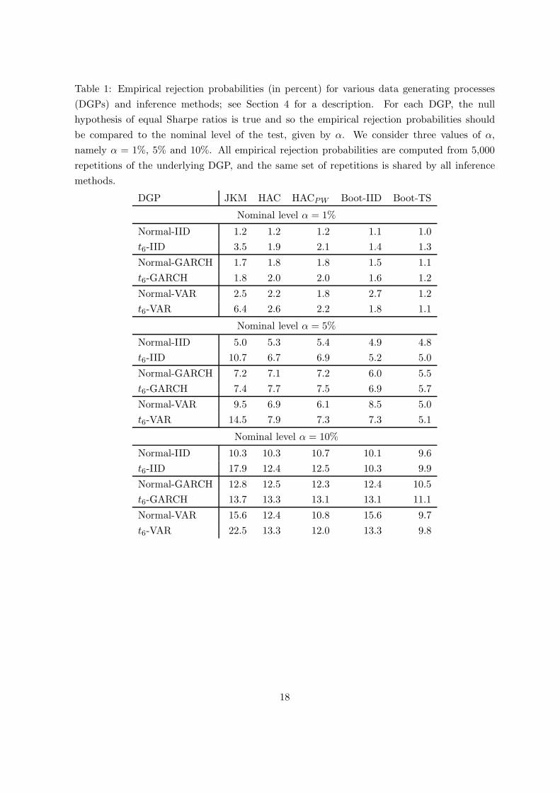
Table 1: Empirical rejection probabilities (in percent) for various data generating processes
(DGPs) and inference methods; see Section 4 for a description. For each DGP, the null
hypothesis of equal Sharpe ratios is true and so the empirical rejection probabilities should
be compared to the nominal level of the test, given by α. We consider three values of α,
namely α = 1%, 5% and 10%. All empirical rejection probabilities are computed from 5,000
repetitions of the underlying DGP, and the same set of repetitions is shared by all inference
methods.
DGP JKM HAC HACPW Boot-IID Boot-TS
Nominal level α = 1%
Normal-IID 1.2 1.2 1.2 1.1 1.0
t6-IID 3.5 1.9 2.1 1.4 1.3
Normal-GARCH 1.7 1.8 1.8 1.5 1.1
t6-GARCH 1.8 2.0 2.0 1.6 1.2
Normal-VAR 2.5 2.2 1.8 2.7 1.2
t6-VAR 6.4 2.6 2.2 1.8 1.1
Nominal level α = 5%
Normal-IID 5.0 5.3 5.4 4.9 4.8
t6-IID 10.7 6.7 6.9 5.2 5.0
Normal-GARCH 7.2 7.1 7.2 6.0 5.5
t6-GARCH 7.4 7.7 7.5 6.9 5.7
Normal-VAR 9.5 6.9 6.1 8.5 5.0
t6-VAR 14.5 7.9 7.3 7.3 5.1
Nominal level α = 10%
Normal-IID 10.3 10.3 10.7 10.1 9.6
t6-IID 17.9 12.4 12.5 10.3 9.9
Normal-GARCH 12.8 12.5 12.3 12.4 10.5
t6-GARCH 13.7 13.3 13.1 13.1 11.1
Normal-VAR 15.6 12.4 10.8 15.6 9.7
t6-VAR 22.5 13.3 12.0 13.3 9.8
18
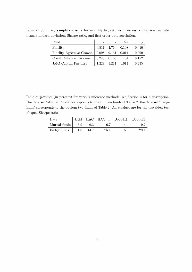
Table 2: Summary sample statistics for monthly log returns in excess of the risk-free rate:
mean, standard deviation, Sharpe ratio, and first-order autocorrelation.
Fund r s Sh φ
Fidelity 0.511 4.760 0.108 −0.010
Fidelity Agressive Growth 0.098 9.161 0.011 0.090
Coast Enhanced Income 0.245 0.168 1.461 0.152
JMG Capital Partners 1.228 1.211 1.014 0.435
Table 3: p-values (in percent) for various inference methods; see Section 4 for a description.
The data set ‘Mutual Funds’ corresponds to the top two funds of Table 2; the data set ‘Hedge
funds’ corresponds to the bottom two funds of Table 2. All p-values are for the two-sided test
of equal Sharpe ratios.
Data JKM HAC HACPW Boot-IID Boot-TS
Mutual funds 3.9 6.3 6.7 4.4 9.2
Hedge funds 1.0 14.7 25.4 5.8 29.4
19

2 4 6 8 10
0.92
0.93
0.94
0.95
0.96
0.97
0.98
Estimated calibration functions
Block size
Estim
ated
cove
rage
Mutual fundsHedge funds
Figure 1: Estimated calibration functions for the two empirical applications. The nominal
level is 1 − α = 0.95. The resulting estimated optimal block sizes are b = 4 for the mutual
funds application and b = 6 for the hedge funds application.
20