robust lpv control for wind turbines - aerospace …seilercontrol/thesis/2016/wang...robust lpv...
TRANSCRIPT

Robust LPV Control for Wind Turbines
A THESIS
SUBMITTED TO THE FACULTY OF THE GRADUATE SCHOOL
OF THE UNIVERSITY OF MINNESOTA
BY
Shu Wang
IN PARTIAL FULFILLMENT OF THE REQUIREMENTS
FOR THE DEGREE OF
DOCTOR OF PHILOSOPHY
Peter J. Seiler, Advisor
July 2016

c© Shu Wang 2016

Acknowledgments
I would like to thank all the people who supported and helped me through the years. It is
a long way with joys and pains to get the PhD degree and I would never have been able to
make it alone. First of all, I want to thank my advisor Peter Seiler. I am grateful for the
time you spent advising me on research, on scientific writing and presentations, etc. None
of my work would have been done without your guidance. It is your advising that shaped
my thoughts on how to solve problems rigorously and efficiently as a Doctor of Philosophy.
I would like to thank my prelim and final oral exams’ committee members, Zongxuan
Sun, Rajesh Rajamani, Andrew Lamperski and Mihailo Jovanovic. I want to express my
gratitude for your comments and suggestions on my research and thesis. I would also like to
thank my collaborators Harald Pfifer and Daniel Ossmann, for the time we worked together
on IQC theories and wind turbine control problems. I also want to thank all my collegues
and friends in the society of systems and controls, especially Bin Hu, Yongxin Chen and
Sei Zhen Khong. I could never forget the discussions we had on research and all other
interesting topics in the past few years.
Finally, I want to thank my parents for supporting and understanding me all these years. For
sure I will find a girlfriend sooner or later (I can not stop laughing at this moment). I would
also like to acknowledge my gratitude to the Solie’s family for hosting me in Minnesota.
There were so many good memories with you and all other friends that made me feel the
warm of home in a country of different language and culture.
i

Dedication
To My Family
ii

Abstract
This thesis proposes a uniform multi-input, multi-output (MIMO) control framework for
wind turbines using the robust linear parameter varying (LPV) design method. This frame-
work is built on an LPV model of the wind turbine, which has a parametric dependence on
the trim wind speed. It takes multiple objectives in different wind conditions into a system-
atic consideration. Therefore, existing results based on single-input, single-output (SISO)
linear control design can be integrated together with stability and performance guarantees.
The proposed design has a uniform structure that covers turbine operations in all wind con-
ditions and provides better load reduction performance than the baseline controller. This
MIMO control architecture can also be extended for active power control (APC) purposes.
Therefore, the wind turbine is capable of providing ancillary services to maintain reliability
of power grids.
The control design in this thesis takes a robust LPV approach. Specifically, this thesis pro-
poses a robust synthesis algorithm for LPV systems using the theory on integral quadratic
constraints (IQCs). This algorithm is a coordinate-wise descent similar to the well-known
DK iteration for µ synthesis. It alternates between an LPV synthesis step and an IQC
analysis step. Both steps can be efficiently solved as semidefinite programs. It is shown
that the proposed algorithm ensures that the robust performance is non-increasing at each
iteration step. Therefore, this algorithm is used in this thesis to synthesize a robust LPV
controller for wind turbines to provide APC. Robust performance of this controller has been
verified using high fidelity simulations. Applications of this method will be various and not
limited to wind turbines.
iii

Contents
List of Figures vii
List of Tables x
Chapter 1 Introduction 1
1.1 Thesis Overview . . . . . . . . . . . . . . . . . . . . . . . . . . . . . . . . . 3
1.2 Thesis Contributions . . . . . . . . . . . . . . . . . . . . . . . . . . . . . . . 4
Chapter 2 Wind Turbine Modeling and Control 6
2.1 Overview of Turbine Operation and Control . . . . . . . . . . . . . . . . . . 6
2.2 Low Fidelity Model . . . . . . . . . . . . . . . . . . . . . . . . . . . . . . . . 10
2.3 High Fidelity Model . . . . . . . . . . . . . . . . . . . . . . . . . . . . . . . 11
2.3.1 Model Description . . . . . . . . . . . . . . . . . . . . . . . . . . . . 11
2.3.2 Model Linearization . . . . . . . . . . . . . . . . . . . . . . . . . . . 13
2.3.3 Multi-Blades Coordinate Transformation . . . . . . . . . . . . . . . 15
2.4 Actuators and Sensors . . . . . . . . . . . . . . . . . . . . . . . . . . . . . . 19
2.4.1 Actuators . . . . . . . . . . . . . . . . . . . . . . . . . . . . . . . . . 19
2.4.2 Sensors . . . . . . . . . . . . . . . . . . . . . . . . . . . . . . . . . . 20
2.5 Baseline Control of Wind Turbines . . . . . . . . . . . . . . . . . . . . . . . 21
iv

Chapter 3 LPV Control for Traditional Operations 23
3.1 Motivation . . . . . . . . . . . . . . . . . . . . . . . . . . . . . . . . . . . . 23
3.2 Induced L2 Control of LPV Systems . . . . . . . . . . . . . . . . . . . . . . 25
3.3 Structure of The Proposed LPV Control System . . . . . . . . . . . . . . . 29
3.4 LPV Design . . . . . . . . . . . . . . . . . . . . . . . . . . . . . . . . . . . . 31
3.4.1 LPV Model Construction . . . . . . . . . . . . . . . . . . . . . . . . 31
3.4.2 Weights Tuning . . . . . . . . . . . . . . . . . . . . . . . . . . . . . . 33
3.4.3 Synthesis Results . . . . . . . . . . . . . . . . . . . . . . . . . . . . . 37
3.5 Simulations and Analysis . . . . . . . . . . . . . . . . . . . . . . . . . . . . 43
3.5.1 Simulation Results . . . . . . . . . . . . . . . . . . . . . . . . . . . . 43
3.5.2 Damage Equivalent Load Analysis . . . . . . . . . . . . . . . . . . . 47
Chapter 4 Robust Synthesis for LPV Systems Using IQCs 52
4.1 Introduction . . . . . . . . . . . . . . . . . . . . . . . . . . . . . . . . . . . . 52
4.2 Integral Quadratic Constraints . . . . . . . . . . . . . . . . . . . . . . . . . 54
4.3 Robust Synthesis Algorithm . . . . . . . . . . . . . . . . . . . . . . . . . . . 56
4.3.1 Problem Formulation . . . . . . . . . . . . . . . . . . . . . . . . . . 56
4.3.2 DK Synthesis . . . . . . . . . . . . . . . . . . . . . . . . . . . . . . . 59
4.3.3 Algorithm Description . . . . . . . . . . . . . . . . . . . . . . . . . . 60
4.4 Technical Details . . . . . . . . . . . . . . . . . . . . . . . . . . . . . . . . . 62
4.4.1 Robust Performance Condition . . . . . . . . . . . . . . . . . . . . . 62
4.4.2 Scaled System . . . . . . . . . . . . . . . . . . . . . . . . . . . . . . 67
4.4.3 Main Theorem . . . . . . . . . . . . . . . . . . . . . . . . . . . . . . 71
4.5 Numerical Example . . . . . . . . . . . . . . . . . . . . . . . . . . . . . . . . 72
v

4.5.1 Comparison to Standard DK Synthesis . . . . . . . . . . . . . . . . . 73
4.5.2 Robust LPV Synthesis . . . . . . . . . . . . . . . . . . . . . . . . . . 74
Chapter 5 Robust LPV Design for Active Power Control 79
5.1 Motivation . . . . . . . . . . . . . . . . . . . . . . . . . . . . . . . . . . . . 79
5.2 Control Strategy Development . . . . . . . . . . . . . . . . . . . . . . . . . 80
5.3 Robust LPV Design . . . . . . . . . . . . . . . . . . . . . . . . . . . . . . . 82
5.3.1 Uncertain LPV Model Construction . . . . . . . . . . . . . . . . . . 83
5.3.2 Weights Tuning . . . . . . . . . . . . . . . . . . . . . . . . . . . . . . 86
5.3.3 Synthesis Results . . . . . . . . . . . . . . . . . . . . . . . . . . . . . 87
5.4 Simulations and Analysis . . . . . . . . . . . . . . . . . . . . . . . . . . . . 92
5.4.1 Simulations for APC . . . . . . . . . . . . . . . . . . . . . . . . . . . 92
5.4.2 Worst Case Performance Simulations . . . . . . . . . . . . . . . . . . 94
Chapter 6 Conclusions 97
Bibliography 99
Appendix A IQC Factorizations 109
Appendix B Extended System State Matrices 112
Appendix C Proof of Lemma 1 113
vi

List of Figures
1.1 World total installed capacity of wind [1]. . . . . . . . . . . . . . . . . . . . 1
2.1 Clipper Liberty C96 2.5 MW wind turbine in University of Minnesota [2]. . 7
2.2 Wind turbine structure and components [3]. . . . . . . . . . . . . . . . . . . 8
2.3 The contour of Cp for the C96 2.5 MW wind turbine. . . . . . . . . . . . . . 9
2.4 Operation regions for the C96 2.5 MW wind turbine. . . . . . . . . . . . . . 10
2.5 One state model of wind turbine. . . . . . . . . . . . . . . . . . . . . . . . . 11
2.6 Effects of blade tip forces in the non-rotating frame. . . . . . . . . . . . . . 16
2.7 Entry values in the 1-st column of A(ψ) and Anr(ψ). . . . . . . . . . . . . . 19
2.8 Bode magnitude plots of the identified model Gid(s), averaged LTI models
G(s) (before MBC) and Gnr(s) (after MBC). . . . . . . . . . . . . . . . . . 20
3.1 Structure of the LPV controller for traditional operations. . . . . . . . . . . 29
3.2 Trim values for linearization. . . . . . . . . . . . . . . . . . . . . . . . . . . 32
3.3 The augmented system for LPV synthesis. . . . . . . . . . . . . . . . . . . . 34
3.4 Bode magnitude plots of weights. . . . . . . . . . . . . . . . . . . . . . . . . 35
3.5 Upper bound of the induced L2 norm γ with ρ. . . . . . . . . . . . . . . . . 38
3.6 Bode magnitude plots from wind disturbance to some outputs at ρ = 9 m/s. 40
3.7 Bode magnitude plots from wind disturbance to some outputs at ρ = 12 m/s. 41
vii

3.8 Bode magnitude plots from wind disturbance to some outputs loads at ρ =
18 m/s. . . . . . . . . . . . . . . . . . . . . . . . . . . . . . . . . . . . . . . . 42
3.9 Simulations for the baseline controller and the LPV controller at 8 m/s. . . 44
3.10 Comparison of power generations for the baseline controller and the LPV
controller in different wine speeds. . . . . . . . . . . . . . . . . . . . . . . . 45
3.11 Simulations for the baseline controller and the LPV controller at 12 m/s. . . 46
3.12 Simulations for the baseline controller and the LPV controller at 18 m/s. . . 48
3.13 Comparison of RMS of the generator speed tracking error for the baseline
controller and the LPV controller in Region 3. . . . . . . . . . . . . . . . . . 49
3.14 Damage equivalent loads (DELs) for the baseline controller and the LPV
controller at different wind speeds. . . . . . . . . . . . . . . . . . . . . . . . 50
3.15 Improvements for the LPV controller on load reduction at different wind
speeds. . . . . . . . . . . . . . . . . . . . . . . . . . . . . . . . . . . . . . . . 51
4.1 Graphical interpretation of the IQC. . . . . . . . . . . . . . . . . . . . . . . 55
4.2 Interconnection for LPV robust synthesis. . . . . . . . . . . . . . . . . . . . 57
4.3 LFT interconnection of Scaled System, Gsclρ . . . . . . . . . . . . . . . . . . . 62
4.4 Uncertain LPV system extended to include filter Ψ1/γ . . . . . . . . . . . . . 63
4.5 LFT interconnection of Hρ and Ψ†λ. . . . . . . . . . . . . . . . . . . . . . . . 70
4.6 Synthesis interconnection for the numerical example. . . . . . . . . . . . . . 73
4.7 Step responses for Knom and Krob. . . . . . . . . . . . . . . . . . . . . . . . 77
5.1 Operation envelope for APC. . . . . . . . . . . . . . . . . . . . . . . . . . . 81
5.2 The proposed LPV controller for APC. . . . . . . . . . . . . . . . . . . . . . 83
5.3 Trim points for APC design. . . . . . . . . . . . . . . . . . . . . . . . . . . . 85
5.4 Uncertain LPV model of wind turbine. . . . . . . . . . . . . . . . . . . . . . 86
5.5 Augmented system for APC design. . . . . . . . . . . . . . . . . . . . . . . 87
5.6 Bode magnitude plots of the sensitivity function from δPcmd to δPe. . . . . 89
viii

5.7 Worst case gain analysis for the robust controller Krob and the nominal con-
troller Knom. . . . . . . . . . . . . . . . . . . . . . . . . . . . . . . . . . . . 90
5.8 Disk margins analysis for the robust controller Krob and the nominal con-
troller Knom at different trim wind speeds. . . . . . . . . . . . . . . . . . . . 91
5.9 Simulations for APC using the robust controller Krob and the nominal con-
troller Knom at ρ = 9 m/s. . . . . . . . . . . . . . . . . . . . . . . . . . . . . 93
5.10 Simulation for APC using the robust controller Krob and the nominal con-
troller Knom at ρ = 18 m/s. . . . . . . . . . . . . . . . . . . . . . . . . . . . 95
5.11 Error on the power output with ∆wc using the robust controller Krob and
the nominal controller Knom. . . . . . . . . . . . . . . . . . . . . . . . . . . 96
ix

List of Tables
2.1 Basics of the C96 2.5 MW wind turbine. . . . . . . . . . . . . . . . . . . . . 7
2.2 Mapping of np terms from the rotating frame by MBC. . . . . . . . . . . . 17
2.3 Trim conditions of the C96 2.5 MW wind turbine for linearization. . . . . . 18
3.1 Weights at different trim points. . . . . . . . . . . . . . . . . . . . . . . . . 36
4.1 LTI robust synthesis results. . . . . . . . . . . . . . . . . . . . . . . . . . . . 74
4.2 LPV robust synthesis results. . . . . . . . . . . . . . . . . . . . . . . . . . . 76
5.1 Iteration process for the robust LPV controller. . . . . . . . . . . . . . . . . 88
5.2 Performance degradation with ∆wc. . . . . . . . . . . . . . . . . . . . . . . 96
x

Chapter 1
Introduction
Wind power is a promising renewable green energy for its zero fuel cost, zero emissions and
abundant sources. With advancements in technology, wind power is increasing very fast all
over the world. Figure 1.1 shows world installed capacity of wind from 1997 to 2012 [1].
Though it only met 3 % of the electricity demand globally in 2012, the penetration of wind
power is very high in some European countries [4]. In the United States, the amount of wind
power is expected to increase to about 20 % of the electricity supply by 2030 [5, 6]. Corre-
spondingly, most states of U.S. have renewable portfolio standards, with wind an important
part of it. According to National Renewable Energy Laboratory’s (NERL) research [7],
estimated U.S. electricity demand in 2050, under some assumptions and constraints, could
be met with 80 % generation from renewable energy (wind, solar and hydroelectric, etc.).
In that scenario, wind will be able to provide about 40% of overall generation.
Figure 1.1: World total installed capacity of wind [1].
1

The rapid growth of wind power requires the wind industry to further minimize costs and
maximize profits in energy markets. These objectives bring several challenges to the control
system of a single utility scale wind turbine, as it has a significant effect on the turbine
performance. Therefore, this thesis is focused on the control design for wind turbines.
Traditionally, the wind turbine control system is designed to maximize the power genera-
tion from available energy in the wind and minimize structural loads of turbine components.
The trade-off between these two objectives is typically achieved by using a mode-dependent
controller which contains two independent control loops to achieve distinct objectives in
different wind speed regions. This baseline controller has been widely accepted by the in-
dustry. However, as the size of wind turbines grows and the structure becomes more flexible,
considerations on load reduction are more critical for larger wind turbines. Therefore, extra
control loops were proposed to improve the load reduction performance, such as individual
pitch control [8, 9], tower and drive train dampers [10–13]. Though these methods signifi-
cantly decreased the turbine loads, the control system structure became more complicated.
There are also other concerns, such as potential dynamic couplings between different control
loops that might affect system performance and stability.
The second challenge for turbine control systems comes from the dynamics variation and
uncertainties in the turbine model. Traditional control system design for wind turbines
usually takes a linear time invariant (LTI) approach since LTI control theory has been well
developed and design tools are simple and reliable for applications [14, 15]. Though some
other controllers such as individual pitch control are implemented in the form of linear time
varying systems, they are still designed in the framework of LTI systems [9, 16]. However,
the performance with an LTI design is difficult to guarantee as the capacity of utility
scaled turbines increase. Larger capacity of turbine usually indicates larger size and more
flexibility, which lead to larger variation of system dynamics in different wind conditions.
At the same time, there are also concerns on robustness in the control design. Though high
fidelity simulation environments like FAST [17] provide relatively accurate model of the
turbine for control design, the real dynamics of the turbine might be subject to different
uncertainties that will significantly degrade the control performance or even lead instability
of the system.
Another challenge for turbine control systems comes from the updated requirements of
power grids. Traditional turbine control systems attempt to maximize the power generation
from available energy in the wind. The power output of wind turbines is therefore variable
due to time-varying wind speeds and it may cause unreliable operation of the power grid.
This is not a significant issue when wind power is only a small portion of the total electricity
generated on the grid. However, to integrate higher levels of variable wind power into the
grid it is important for wind turbines to provide ancillary services to help maintain the
2

reliability of power grids. Ancillary services require wind turbines to provide active power
control (APC) [4]. Therefore, it is important to improve the traditional turbine control
system for APC purposes.
1.1 Thesis Overview
To address all these issues as mentioned above, this thesis proposes a uniform multi-input,
multi-output (MIMO) control framework for wind turbines using the robust linear param-
eter varying (LPV) design method. The contents in each chapter of the thesis are briefly
introduced as follows.
Chapter 2 gives an overview of wind turbine modeling and controls. It covers the basics on
the Clipper Liberty C96 2.5 MW wind turbine, which is the research focus of this thesis. The
operations of wind turbine in different wind speeds and objectives for its control system
are also introduced here. The modeling of wind turbines starts from a brief review of a
simple nonlinear one state model that captures the aerodynamics and rotor dynamics of
the turbine. To cover the structural dynamics of the turbine, a high fidelity model is also
presented. This high fidelity model is integrated in the FAST simulation package [17] and
can be linearized for advanced control design purposes. This chapter also briefly reviews
the actuators and sensors used for control of wind turbines. In the end, a baseline controller
which has been widely accepted in industry is presented.
In Chapter 3, a uniform MIMO control architecture that covers all wind conditions will be
first proposed. This LPV controller is able to maximize the power generation in Region 2
and track the rated generator speed in Region 3. Considerations on load reduction will also
be parts of the design. The recently developed LPV toolbox in Matlab [18] will be used
to synthesize the LPV controller. This uniformly designed controller allows the turbine
to meet objectives in different wind conditions and ensures a smooth transition between
different wind speed regions. Performance of this LPV controller will be further verified by
high fidelity simulations in FAST and post analysis.
In Chapter 4, the theory of integral quadratic constraints (IQCs) [19] will be applied to
develop a robust synthesis algorithm for a class of uncertain LPV systems. The uncertain
system is described as an interconnection of a nominal (not-uncertain) gridding based LPV
system and a block structured uncertainty. The input/output behavior of the uncertainty
is described by IQCs. The robust synthesis problem leads to a non-convex optimization
and the proposed algorithm is a coordinate-wise descent which is similar to the well-known
DK iteration for µ synthesis and can be efficiently solved as semidefinite programs. The
effectiveness of the proposed method is demonstrated on a simple numerical example.
3

In Chapter 5, the robust synthesis algorithm as proposed in Chapter 4 will be used to
design an LPV controller to provide APC. The proposed control system architecture can
be considered as an extension of the LPV controller in Chapter 3. The design procedure
is therefore significantly simplified since some of the tuning results in Chapter 3 can be
directly inherited here. In addition, a multiplicative uncertainty is considered in the blade
pitch input channel of the turbine model. The synthesized robust LPV controller shows
similar performance on APC as a nominal LPV controller designed without considerations
of uncertainty. However, the robust controller has much better performance when the worst
case uncertainty is added to the system dynamics.
Chapter 6 is the end of this thesis. Brief conclusions will be made to summarize all works
and contributions in this thesis and provide possible directions for future works.
1.2 Thesis Contributions
This thesis extends theories on robust control for LPV systems and provides a uniform
MIMO control architecture for wind turbines using the robust LPV approach. The contri-
butions of this thesis are listed as follows.
1. LPV Control Framework: This framework as proposed in Chapter 3 is built on
an LPV model of the wind turbine, which has a parametric dependence on the trim
wind speed. It takes multiple objectives in different wind conditions into a systematic
consideration, such that existing results based on single-input, single-output (SISO)
linear control design can be integrated together with stability and performance guar-
antees. Detailed simulations and post analysis show that this LPV controller achieves
similar performance of power capturing as the baseline controller in below rated wind
speed and much better performance of load reduction and generator speed tracking
in above rated wind speed. More importantly, the proposed framework is an open
structure and can be extended in the future to allow more feedback loops for further
load reductions and/or other operations of wind turbines, such as APC.
2. Robust LPV Synthesis: The nominal LPV design, as shown Chapter 3 does not
consider possible uncertainties in the plant. Therefore, the control performance might
be significantly degraded if the system dynamics is perturbed. However, robust syn-
thesis algorithms like µ-synthesis [20] are not directly available for LPV systems and
existing theories for robust LPV control are still incomplete. Chapter 4 proposes
a robust synthesis algorithm for LPV systems using the theories on IQCs. It is a
coordinate-wise descent similar to the well-known DK iteration for µ synthesis. Specif-
ically, the proposed algorithm alternates between an LPV synthesis step and an IQC
4

analysis step. Both steps can be efficiently solved as semidefinite programs. It is shown
that the proposed algorithm ensures that the robust performance is non-increasing at
each iteration step. The effectiveness of the proposed method is demonstrated on a
simple numerical example. Applications of this method are various and not limited
to wind turbines.
3. Robust LPV Design for APC: Chapter 5 proposes an LPV controller to provide
APC using the robust LPV synthesis method presented in Chapter 4. This LPV
controller is developed from the design in Chapter 3 by adding a feedback loop for
the power reference tracking. To ensure robustness of the controller, a multiplica-
tive uncertainty in the blade pitch input channel is considered in the turbine model.
Simulation results show that the robust LPV controller provides fast responses to
the power reference commands and maintains performance even with existence of the
worst case uncertainty. Therefore, it is expected that wind turbines will be able to
participate in ancillary services of power grids by providing APC. This will greatly
improve the competitiveness of wind in the energy market.
5

Chapter 2
Wind Turbine Modeling and
Control
2.1 Overview of Turbine Operation and Control
The history of extracting energy from wind dates back to the first windmills about 3000
years ago [8]. Windmills were used to take energy from wind for mechanical operations,
such as pumping water or grinding grains. As electricity became a major source of power for
modern industry, wind turbines were built by James Blyth in 1887 [21] and Charles Brush
in 1888 [22] respectively. These turbines consisted of a windmill and a generator to convert
the wind power into electricity. Another milestone in the history of wind power development
was the Smith Putnam wind turbine built in 1941 [23]. As the first wind turbine in history
with a capacity of 1.25 MW, it showed a potential for large scale turbines. Many different
turbine designs have been considered over the past 100 years [8, 24]. The capacity of a
single turbine has also increased from 12 KW to 10 MW [25]. In this thesis, the focus is
on 3-blades, variable speed, horizontal axis, on shore, upwind turbine. This is the most
popular one in wind industry. Commercialized utility scale turbines with this design have
been installed with capacity up to 7.5 MW (E-126 wind turbine designed by Enercon in
Germany [25], which has a hub height of 135 m and a rotor diameter of 126 m).
The specific model that will be studied in this thesis is the Clipper Liberty C96 2.5 MW
wind turbine which is located in UMore Park, Rosemount, MN, as shown in Figure 2.1.
This turbine is owned by EOLOS Wind Energy Research Consortium at University of
Minnesota [2] for research purposes. The author of this thesis therefore has access to the
high fidelity model, the baseline controller and real time operational data of this turbine.
Basics of the C96 turbine are shown in Table 2.1.
6

Figure 2.1: Clipper Liberty C96 2.5 MW wind turbine in University of Minnesota [2].
Table 2.1: Basics of the C96 2.5 MW wind turbine.Hub height 80.4 m
Rotor radius 48 mWind speed range for operation 4 ∼ 25 m/s
Rated rotor speed 15.49 RPMRated generator torque 23473 N ·m
Rated power 2.5 MW
Figure 2.2 shows the common structure and components of the above described type of wind
turbine [3]. As the wind flow passes through the rotor plane of the turbine, lift is generated
on blades and leads to the rotation of the low speed rotor shaft. The aerodynamic torque
generated on the low speed rotor shaft transmits to the high speed generator shaft through
the gearbox and the generator converts mechanical energy of the rotation into electrical
energy. The low speed shaft, gearbox, high speed shaft and generator are all installed
inside the nacelle, which is mounted on top of the turbine tower.
The control of wind turbines relies on some actuators. As shown in Figure 2.2, the yaw
motor is used in the upwind turbine to rotate the nacelle such that the rotor plane faces the
direction of the incoming wind flow for maximizing the power capturing. Other actuators
that are commonly used for turbine control are the blade pitch and generator torque. The
servo motor installed at the root of each blade is used to pitch the blade and change the
lift force generated on the blade. The generator torque is used to change the power output
and generator speed. Details on turbine actuators will be provided in Section 2.4.1.
Sensors are necessary for the turbine control and monitoring. For example, sensors on
the drive train (which includes the low speed rotor shaft, high speed generator shaft and
gearbox) are used to measure the rotor speed and/or generator speed for the closed loop
7

Figure 2.2: Wind turbine structure and components [3].
feedback control of wind turbines. Another sensor that is widely used on wind turbines
is the anemometer (as shown in Figure 2.2), which usually sits on the top of the nacelle.
However, the wind speed measurement from the anemometer is corrupted by the rotation of
blades and it is therefore limited for control purposes. Modern wind turbines also have some
other sensors for monitoring states and loads of the turbine and improving the performance
of turbine control systems, which will be further discussed in Section 2.4.2.
The captured power of a wind turbine is given by
Pc =1
2Cp(β, λ)ρArv
3 (2.1)
where ρ is the air density [kg/m3], Ar := πR2 is the swept area of rotor blades perpendicular
to the wind flow [m2], R is the radius of the rotor area [m], and v is the wind speed
[m/s] [8,26]. The non-dimensional power coefficient Cp is the fraction of the available wind
power captured by the turbine. The power coefficient is a function of the (collective) blade
pitch angle β [deg] and the tip speed ratio λ [unitless]. The tip speed ratio is defined as
the ratio λ := Rωv where ω is the rotor speed [rad/s]. In words, λ is defined as the blade
tip tangential velocity divided by the wind speed. Figure 2.3 shows the contour of Cp as
a function of β and λ (contours with values less than or equal to 0 have been removed
from the plot). It is generated for the above mentioned C96 2.5 MW wind turbine and Cp
achieves its maximal value at β∗ = 1.6 deg and λ∗ = 8.4. This maximum value Cp∗ might
8

be varying from one turbine to another. However, there is a theoretical upper bound for
Cp∗ that is equal to 16/27. This upper bound is known as Betz limit after the German
aerodynamicist Albert Betz [8]. Here, the Cp∗ for the C96 turbine is also below the Betz
limit but the exact value is not provided for proprietary reasons.
−10 −5 0 5 10 15 20 25 30
5
10
15
20
Blade pitch angle β [deg]
Tip
spee
dra
tioλ
[un
itle
ss]
0.1
0.2
0.3
0.4
Figure 2.3: The contour of Cp for the C96 2.5 MW wind turbine.
The objectives of the wind turbine control are to maximize the power generation from avail-
able energy in the wind and minimize structural loads of turbine components. The trade-off
between these two objectives is typically achieved using a mode-dependent controller with
distinct objectives in different wind speed regions [8, 27, 28]. As shown in Figure 2.4, there
are essentially four operating regions for the turbine in the power versus wind speed curve.
Below the cut-in speed (Region 1), the turbine is kept in a parked, non-rotating state as
there is insufficient energy available from the wind. Above the cut-out speed (Region 4),
the turbine is shut down to prevent structural damages. Between the cut-in and rated
wind speeds (Region 2), the main objective is to maximize the captured power. Between
the rated and cut-out wind speeds (Region 3), the main objective is to maintain the rated
power while minimizing structural loads on the turbine. The transition between Regions 2
and 3 is referred to as Region 2.5. Region 2.5 is introduced because the rated rotor speed
is usually reached before the Region 2 control law reaches the rated torque.
The design of wind turbine controllers requires dynamic models of the wind turbine plant,
actuators and sensors. Details on the modeling and baseline controller design are provided
in following sections. In Section 2.2, a low fidelity, one-state, nonlinear turbine model will be
9

0 2 4 6 8 10 12 14 16 18 20 22 24 26 28 300
1,000
2,000
3,000 Cut-in Rated Cut-out
Region 1 Region 2 Region 3 Region 4
Wind speed v [m/s]
Pow
erP
[kW
]
Figure 2.4: Operation regions for the C96 2.5 MW wind turbine.
introduced that captures the rotor dynamics. In Section 2.3, a high fidelity nonlinear wind
turbine model from FAST [17] will be explained. This high fidelity model includes more
detailed structural dynamics of the turbine and it is therefore suitable for advanced control
design and simulation purposes. Linearization of the FAST model and post-processing of the
linearized model will also be explained in this section. Section 2.4 will discuss actuator and
sensor dynamics. In Section 2.5, a baseline controller for wind turbines will be presented.
2.2 Low Fidelity Model
This section provides a one-state, nonlinear model of a wind turbine that captures the
steady state aerodynamics and the rigid body rotor dynamics [29]. This low fidelity mod-
el does not contain structural dynamics of the turbine, such as vibrations of tower and
blades. Therefore, it is usually used when loads on the tower and blades are not considered.
However, this simplified model is helpful for understanding basic principles of the turbine
operation.
Figure 2.5 shows a diagram of this one-state model. The lift force generated on blades leads
to the aerodynamic torque τa on the low speed rotor shaft. It is balanced by the generator
torque τg on the other side of the drive train. Considering all rotating parts of the turbine
as a rigid body, which includes the blades, hub and drive train, the rotor dynamics can be
expressed as comprehensive effects of τa and τg:
Jω = τa −Nτg (2.2)
where τa and τg [N ·m] are aerodynamic and generator torques on the drive train. J [kg ·m2]
is the inertia of all rotating parts, including the blades, hub and drive train. ω [rad/s] is the
10
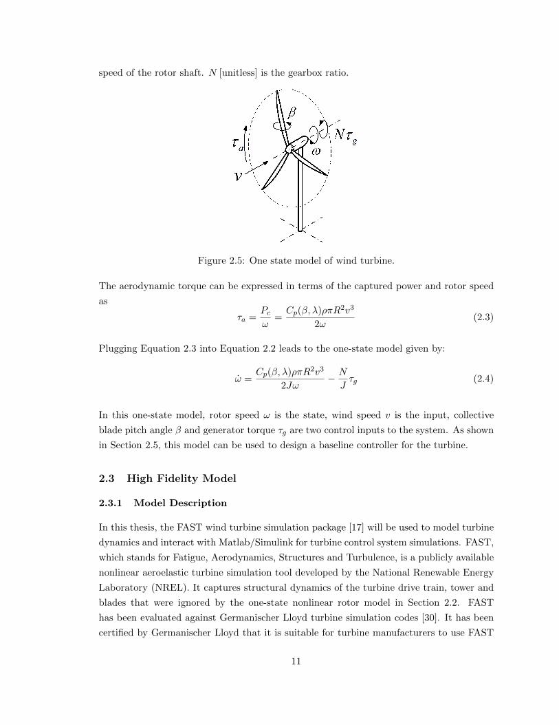
speed of the rotor shaft. N [unitless] is the gearbox ratio.
Figure 2.5: One state model of wind turbine.
The aerodynamic torque can be expressed in terms of the captured power and rotor speed
as
τa =Pcω
=Cp(β, λ)ρπR2v3
2ω(2.3)
Plugging Equation 2.3 into Equation 2.2 leads to the one-state model given by:
ω =Cp(β, λ)ρπR2v3
2Jω− N
Jτg (2.4)
In this one-state model, rotor speed ω is the state, wind speed v is the input, collective
blade pitch angle β and generator torque τg are two control inputs to the system. As shown
in Section 2.5, this model can be used to design a baseline controller for the turbine.
2.3 High Fidelity Model
2.3.1 Model Description
In this thesis, the FAST wind turbine simulation package [17] will be used to model turbine
dynamics and interact with Matlab/Simulink for turbine control system simulations. FAST,
which stands for Fatigue, Aerodynamics, Structures and Turbulence, is a publicly available
nonlinear aeroelastic turbine simulation tool developed by the National Renewable Energy
Laboratory (NREL). It captures structural dynamics of the turbine drive train, tower and
blades that were ignored by the one-state nonlinear rotor model in Section 2.2. FAST
has been evaluated against Germanischer Lloyd turbine simulation codes [30]. It has been
certified by Germanischer Lloyd that it is suitable for turbine manufacturers to use FAST
11

simulations for wind turbine performance certifications.
In FAST, the drive train, tower and blades are treated as flexible structures. The drive train
torsional flexibility is modeled as a linear inertia-spring-damper system. Deformations of the
tower and blades are approximated with the assumed modes method [31,32]. To apply this
method, the tower and blades are treated as cantilever beams with properties varying along
their length. These properties are specified at desired points on the tower and blades. Linear
interpolation is used between these points. For example, airfoil properties and the mass
distribution of the blade can be specified along the blade length. Deformations of the tower
and blades are approximated by superposition of basis functions known as mode shapes.
Each mode shape corresponds to a particular deformation shape and is defined as one
degree of freedom. Though there are couplings between all structure modes, it is assumed
in this method that the effect of couping is small and does not affect the model response.
Therefore, each mode shape of the tower and blades can be calculated independently based
on properties of structures.
The FAST simulation package can model dynamics of 3-blades onshore wind turbines with
up to 18 degrees of freedom (DOFs). These DOFs are described as follows. There are 4
DOFs for first and second tower bending modes in fore-aft and side-to-side directions. For
each blade, there are 2 DOFs for first and second blade flapwise bending modes and 1 DOF
for the first blade edgewise bending mode. For the drive train, there are 2 DOFs for the
torsion and generator speed. There is 1 DOF for the nacelle yaw motion. 2 more DOFs
account for the rotor and tail furl. There are extra 6 DOFs available for modeling platform
motions of offshore wind turbines. That is up to 24 DOFs.
To simulate the operation of wind turbines and calculate deformations of turbine structures
in FAST, information of the incoming wind flow in front of the turbine rotor and calculation
of aerodynamic loads generated on turbine models are necessary. An accurate model of the
incoming wind flow can be solved by computational fluid dynamics (CFD) codes. However,
due to time and computational costs of CFD codes, it is much simpler to use TurbSim [33] to
generate wind flow profiles. TurbSim is a stochastic, turbulent wind simulator developed by
NREL. It is able to generate wind trajectories with various spatial and temporal correlation
models. Some common turbulence models that are defined in IEC-61400-1 standards [34] for
wind turbine testing are also included. Inputs of TurbSim are various turbulence properties.
Its output is a description of the turbulent wind field as a function of time on the turbine
rotor. There are two options of fidelity for wind field descriptions. In the first option which is
called the hub-height wind profile, it is assumed that turbulence properties are the same all
over the rotor by averaging the wind data on the hub height. The wind profile is described
by 7 parameters as functions of time. This option is suitable for the linearization of turbine
models and control oriented analysis and design. In the second option which is called the
12
full-field wind profile, the turbulence has spatial variations over the rotor. Therefore the
wind profile is described by detailed wind speed data in three directions as function of
time on a raster grid over the rotor. It provides a more realistic modeling of the wind
field by capturing spatial variations of the wind field. It is therefore suitable for simulation
purposes. These pre-calculated wind trajectories can be used by FAST for calculations of
aerodynamic loads. This is achieved in FAST by integrating with the AeroDyn code [35],
which is also developed by NREL. AeroDyn uses blade element momentum theory [36] to
calculate aerodynamic forces and moments. FAST, AeroDyn and TurbSim codes are of
sufficient fidelity for control design and simulation purposes. Therefore, they are adopted
in this thesis.
The dynamics of wind turbines are essentially nonlinear. This nonlinear wind turbine model
in FAST can be expressed as
q = f(q, q, d, u, t)
y = g(q, q, d, u, t)(2.5)
where q ∈ Rnq and q ∈ Rnq are the turbine states. As described above, there are up to 24
DOFs available in FAST. Therefore the maximum value for nq is 24. For simplicity, however,
it is common to disable some DOFs in FAST to obtain a lower order nonlinear or linear
model for simulations or control design. u ∈ R5 is the control input vector which includes
the generator torque, individual pitch angles for three blades and yaw angle. y ∈ Rny
is the measurement vector and its dimension depends on chosen outputs. A full list of
available outputs in FAST can be found in [17]. d ∈ R7 is the wind disturbance input
which consists of the hub-height average wind speed, horizontal wind direction, vertical
wind speed, horizontal wind shear, vertical power law wind shear, linear vertical wind shear
and horizontal hub-height wind gust. This is the simplified wind field description in FAST.
The 7 disturbance inputs in this simplified description correspond to the 7 parameters in
the hub height wind profile generated by TurbSim. In contrast, the more complex full-field
wind description in TurbSim is not suitable for control oriented linearizations in FAST, as
there are much more inputs required to match parameters of the full-field wind profile.
2.3.2 Model Linearization
To apply well established linear control techniques, the FAST simulation package provides
an option to generate linear system approximations of nonlinear wind turbine dynamics.
The linearization in FAST is started by first simulating the nonlinear turbine model under
steady wind conditions until it reaches a trim operating trajectory q(t). Therefore, the wind
disturbance input and control inputs are held constant at trim values d and u specified by
users in the simulation. The resulting trim trajectory q(t) is periodic with the trim rotor
13

rotation period T , i.e. q(t) = q(t+ T ), and satisfies
¨q = f( ˙q, q, d, u, t)
y = g( ˙q, q, d, u, t)(2.6)
The nonlinear model in Equation 2.5 is linearized around q(t) through numerical perturba-
tions [17] and a periodic linear time varying (PLTV) model is generated with state space
equations as
δx = A(q(t))δx +Bd(q(t))δd +Bu(q(t))δu
δy = C(q(t))δx +Dd(q(t))δd +Du(q(t))δu(2.7)
Where
δx(t) :=
[δq(t)
δq(t)
]=
[q(t)− q(t)q(t)− ˙q(t)
]δd(t) := d(t)− d
δu(t) := u(t)− u
δy(t) := y(t)− y(t)
(2.8)
The dimensions of δx(t), δd(t), δu(t) and δy(t) directly follow from the state, input and
output signal dimensions in Equation 2.6. Since the trim trajectory q(t) is periodic with
the rotor rotation period T , the state space equations of the model in Equation 2.7 are also
periodic with the same period.
As control techniques for linear time invariant (LTI) systems are mature and common in
theory and practice, it is desirable to approximate the PLTV model in Equation 2.7 by an
LTI one. There are several approaches available to generate the approximated LTI mod-
el. The simplest methods are to evaluate the PLTV model at a fixed rotor position or to
average state space matrices of the PLTV model over one rotor period. However, these
methods ignore periodic properties of the system and typically do not provide an approxi-
mated LTI model with sufficient accuracy. Another approach is developed based on Floquet
theory [37,38]. It converts a PLTV system into a system with a constant state “A” matrix
by using a time varying coordinate transformation. The Floquet transformation retains pe-
riodic properties of the system but loses the physical intuition on system states. The most
common approach in the wind turbine industry is to use the multi-blade coordinate (MBC)
transformation [39–41] to generate a weakly PLTV system from the original one. An LTI
model is therefore approximated by averaging the weakly PLTV system without losing too
many periodic properties. This approach is adopted in this thesis for model based control
design of wind turbines. Details on the MBC transformation will be given in Section 2.3.3.
14

2.3.3 Multi-Blades Coordinate Transformation
The nonlinear and linear wind turbine models (Equation 2.5 and 2.7) presented in Section-
s 2.3.1 and 2.3.2 are defined in various coordinate systems. Details on these coordinate
systems can be found in [17]. Specifically, the tower, drive train and generator DOFs are
defined in an earth fixed coordinate system while DOFs associated with turbine blades are
defined in a system that rotates with the rotor. As mentioned in Section 2.3.2, the LTI
model approximated by averaging the PLTV model defined in the mixed coordinate system
(both rotating and non-rotating) is not sufficiently accurate as the averaging ignores period-
ic properties of the model. For instance, dynamics of tower motion coupled by blade modes
will be removed in this approach. Therefore, it is desirable to use the MBC transformation
to transform states, inputs and outputs of the model from the mixed coordinate system to
a purely non-rotating coordinate system.
Ideally, the MBC transformation converts the PLTV system into an LTI system. In practice,
however, the transformed system is still “weakly” periodic, i.e. it is periodic but with
significantly less time variation compared to the original PLTV system. An LTI system can
be approximated by averaging state space matrices of the weakly PLTV system over one
rotor period. This approximation LTI model is of sufficient accuracy for control oriented
design purposes.
The MBC transformation is defined by a transformation matrix M : R→ R3×3 as a function
of the rotor position ψ:
M(ψ) =
1 sin(ψ) cos(ψ)
1 sin(ψ + 2π3 ) cos(ψ + 2π
3 )
1 sin(ψ + 4π3 ) cos(ψ + 4π
3 )
(2.9)
For a given rotor position ψ, M(ψ) transforms variables associated with 3 blades from
the non-rotating frame to the rotating frame. Conversely, the inverse of M(ψ) transforms
variables from the rotating frame to the non-rotating frame:
M−1(ψ) =2
3
12
12
12
sin(ψ) sin(ψ + 2π3 ) sin(ψ + 4π
3 )
cos(ψ) cos(ψ + 2π3 ) cos(ψ + 4π
3 )
(2.10)
The MBC transformation has a very straight forward physical interpretation in the appli-
cation of wind turbines. As shown in Figure 2.6, consider a force Fi acting on the tip of
the i-th blade in the direction that is perpendicular to the rotor plane. Assuming that the
rotor position ψ is defined as the azimuth angle of the 1-st blade, ψ+ (i− 1)2π3 is therefore
the azimuth angle for the i-th blade. Applying the inverse MBC transformation to the force
15

F = [ F1 F2 F3 ]T results in the force in the non-rotating frame as Fnr = [ Fnravg Fnryaw Fnrtilt ]T .
The superscript nr denotes variables defined in the non-rotating frame. After the transfor-
mation, these variables have meanings in terms of rotor motion instead of individual blades.
Fnravg is the averaged force of F that causes the rotor to bend as a cone. Fnryaw and Fnrtilt are
the forces resulting in rotor yaw and tilt, respectively [42].
Figure 2.6: Effects of blade tip forces in the non-rotating frame.
The MBC transformation converts the original PLTV model into a “weakly” PLTV model.
This is due to the fact that periodic dynamics of blades usually have a phase shift of 2π3
between each blade. Specifically, assume the force Fi mentioned above is sinusoid Fi =
F0 sin(ψ + (i− 1)2π3 + θ) while θ is an initial phase shift. As the azimuth angle for the i-th
blade is ψ + (i− 1)2π3 , Fi has the same value for the i-th blade at the same azimuth angle.
Performing the MBC transformation on the force
F = F0
sin(ψ + θ)
sin(ψ + 2π3 + θ)
sin(ψ + 4π3 + θ)
(2.11)
results in the force in the non-rotating frame as Fnr = F0 [ 0 cos(θ) sin(θ) ]T which is constant
instead of periodic. In a more general setting, assume qi is the state of the i-th blade that
has the same period as the rotor motion and Fourier series of qi can be expressed as
qi =
∞∑n=0
an sin(n(ψ + (i− 1)2π
3) + θn) (2.12)
After the MBC transformation, the n-th order harmonic term (which is usually called the
16

np term while p stands for the periodic motion of the rotor)
q(n) = an
sin(nψ + θn)
sin(n(ψ + 2π3 ) + θn)
sin(n(ψ + 4π3 ) + θn)
(2.13)
will be converted in the non-rotating frame as qnr(n) = [ qnr(n)avg qnr(n)yaw q
nr(n)tilt
]T . The detailed
value of each entry in qnr(n) depends on the order n and can be generalized as shown in
Table 2.2.
Table 2.2: Mapping of np terms from the rotating frame by MBC.
n qnr(n)avg q
nr(n)yaw q
nr(n)tilt
0 a0 sin θ0 0 01 0 a1 cos θ1 a1 sin θ1
2 0 −a2 cos(3ψ + θ2) a2 sin(3ψ + θ2)... ... ... ...
3k + 0 an sin(3kψ + θn) 0 03k + 1 0 an cos(3kψ + θn) an sin(3kψ + θn)3k + 2 0 −an cos
(3(k + 1)ψ + θn
)an sin
(3(k + 1)ψ + θn
)It can be concluded from Table 2.2 that 0p and 1p terms which are usually dominating
parts in qi will be mapped to constant values in the non-rotating frame. Higher order
harmonic terms in the rotating frame will be mapped to harmonic terms whose orders are
multiples of 3p in the non-rotating frame and result in the “weakly” periodic property due
to insignificant weightings {an}∞n=2 on these terms.
The complete MBC transformation for PLTV systems contains a collection of state, input,
and output transformations which can be derived using results in [39] and the manual
for NREL Matlab utilities that implement the MBC transformation [41]. Applying these
transformations to the PLTV model in Equation 2.7 leads to a weakly PLTV model with
significantly less periodic variation in state space matrices. Averaging the weakly PLTV
system over one rotor period gives an LTI model with sufficient accuracy [40].
The application of the MBC transformation will be shown in the following example. In this
simplified example, consider the C96 wind turbine model with 10 DOFs that include rotor
position, drive train torsion, first tower fore-aft and side-to-side bending modes, and first
flapwise and edgewise bending modes for each blade. The turbine is simulated at a trim
point as shown in Table 2.3.
For simplicity, trim values for wind disturbance inputs d and yaw angle u5 as defined in 2.3.1
are set to 0 except for the hub-height average wind speed d1 = 16 m/s. This is a typical
operation condition in Region 3 as the wind speed is above the rated and the turbine is
17

Table 2.3: Trim conditions of the C96 2.5 MW wind turbine for linearization.Trim variables Values
Hub-height average wind speed 16 m/sRotor speed 15.49 RPM
Generator torque 23473 N ·mBlade pitch angles 14.36 deg
Yaw angle 0 deg
operating at the rated rotor speed and generator torque.
Here, the interest is focused on open loop dynamics from the disturbance input of hub-height
averaged wind speed δd1 to the output of tower side-to-side bending moment δy [kN ·m].
Therefore, all 5 control inputs of δu and the remaining 6 wind disturbance inputs of δd
are disabled. A linearization of the nonlinear FAST model with the interested input and
output yields a SISO (single input single output) PLTV model Gψ as expressed by state
space matrices[A(ψ) B(ψ)C(ψ) D(ψ)
]. Applying the MBC transformation to Gψ results in the PLTV
model Gnrψ with all states in the non-rotating coordinate frame. Define the state space
matrices for Gnrψ as[Anr(ψ) Bnr(ψ)Cnr(ψ) Dnr(ψ)
]. Figure 2.7 shows entry values in the 1-st column of
A(ψ) and Anr(ψ) as functions of ψ in two subplots respectively. It should be noted that
there are 20 entries for each column and some entries overlap with each other in the subplots
as their values are very close. It is seen that some entries in the first column of A(ψ) have
significant variations within one period of ψ while all entries in the 1-st column of Anr(ψ)
have much smaller variations with ψ. Checking entries in other columns or rows of state
space matrices leads to similar comparison results. It is therefore valid to conclude that
Gnrψ is a “weakly” PLTV system.
In the next step, state space matrices of Gψ and Gnrψ are averaged over one rotor period
to generate LTI models G(s) and Gnr(s) respectively. Bode magnitude plots of G(s) and
Gnr(s) are shown in Figure 2.8. As a reference, the grey plot is generated by identifying the
C96 model with the same 10 DOFs enabled in FAST, denoted as Gid(s). This identification
is started by first simulating the model in trim conditions as specified in Table 2.3. The
simulation lasts for 400 s and the output is recorded as y. In the second simulation, a 400 s
chirp signal with small magnitude (±0.5 m/s) is added to the channel of hub-height wind
speed as disturbance δd1 . The frequency of the chirp signal linearly varies from 0.1 rad/s
to 100 rad/s and therefore can be expressed as ω(t) = 0.1 + 100−0.1400 t. Subtracting y from
the output y in the second simulation gives δy. By taking Fourier transforms of δd1 and δy,
the dynamic response of the model in the frequency domain can be identified as Gid(jω) =∆y(jω)∆d1
(jω) . Figure 2.8 shows that Gnr(s) has a much closer frequency response to the identified
model Gid(s). Especially, Gnr(s) and Gid(s) have similar peak magnitudes at 2rad/s, which
corresponds to the 1-st tower side-to-side bending mode. In addition, Gnr(s) and Gid(s)
18

0 100 200 300−5
0
5
10
15
20
ψ [deg]
valu
e
1-st column of A(ψ)
0 100 200 300−5
0
5
10
15
20
ψ [deg]
valu
e
1-st column of Anr(ψ)
Figure 2.7: Entry values in the 1-st column of A(ψ) and Anr(ψ).
both have 2 more peaks at 4.93 rad/s and 8.24 rad/s. These 2 peaks correspond to 2 pairs
of conjugate poles −0.05± 4.93 j and −0.05± 8.24 j introduced by blade edgewise bending
modes in the non-rotating frame. However, this coupling to tower structural dynamics is
lost in G(s) by directly averaging state space matrices of Gψ. Comparisons in Figure 2.7
and 2.8 indicate that the MBC transformation is a necessary step to get an LTI model
with sufficient accuracy for control design purposes.
2.4 Actuators and Sensors
2.4.1 Actuators
As described in Sections 2.1 and 2.3, there are mainly 5 control inputs available for the
control of wind turbines: the generator torque, 3 blade pitch angles and turbine yaw angle.
However, the use of yaw motor is limited to a very low rate (usually less than 1 deg/s)
for avoiding dangerous gyroscopic forces [43]. Due to the slow dynamics of yaw motion,
research on yaw control is not of great interest. In this thesis, the yaw actuator model
will not be considered in the design and the yaw angle is held constant to the direction of
incoming wind flow in simulations.
The dynamics of generator torque actuation is also ignored in this thesis. This is because
19

10−1 100 101 1020
20
40
60
80
100
Frequency [rad/s]
Mag
nit
ud
e[d
B]
Gid(s)
G(s)
Gnr(s)
Figure 2.8: Bode magnitude plots of the identified model Gid(s), averaged LTI models G(s)(before MBC) and Gnr(s) (after MBC).
the power electronics on modern utility scale wind turbines has very small time constant
and the dynamics of generator torque actuation is much faster than the turbine dynamics
of interest [43]. It is reasonable to assume that the generator torque command can be
responded almost immediately for the desired bandwidth. Generator torque is therefore an
effective control input for maximizing the captured power [29] and minimizing the load of
torsion in the drive train [11].
Blade pitch actuators have restrictive bandwidths for wind turbine control systems. The
dynamics of pitch actuators can be modeled as first or second order LTI systems [24].
In addition, there are usually hard bounds on pitch actuation rates. Therefore, these
constraints are considered in cases that the control bandwidth is close to the actuation
limit or the wind turbulence level is high. It should also be noted that the three blade pitch
angles can be controlled collectively or individually, as there is one actuator for each blade.
In this thesis, the collective pitch control is considered.
2.4.2 Sensors
Traditionally, there are two types of sensors that have been used on utility scale wind
turbines. As introduced in Section 2.1, the sensors for rotor speed and/or generator speed
measurements are widely used for the closed loop control of wind turbines. It will be seen
20

in Section 2.5 that the rotor speed measurement is the most important feedback signal for
the baseline controller.
The anemometer is another sensor that wind turbines usually have for wind speed mea-
surements. It is commonly used for supervisory control of wind turbines, e.g. to determine
if the wind speed is sufficient to start the turbine [43]. However, due to the interaction
between the rotor and the wind, anemometers usually can not provide accurate wind speed
measurements. They are therefore limited for applications on the closed loop feedback
control.
Instead, advanced wind speed measurement technology, such as LIDAR, [44, 45] has been
investigated by researchers for improving performance of turbine control systems. Here,
LIDAR stands for light detection and ranging systems. It is capable of measuring the speed
of incoming wind flow before it interacts with the turbine rotor. Advantages of LIDAR
on improving turbine performance have been validated by high fidelity simulations and/or
experiments [46–50]. The use of LIDAR in wind industry is promising as the cost for
installation decreases and the corresponding control system becomes mature. The LIDAR
model can be implemented with the FAST Simulink model by reading turbulent wind files
generated by TurbSim before simulations. In this thesis, the wind speed measurement is
assumed to be available from LIDAR for robust LPV control design.
Other advanced sensors that could be used for monitoring and/or control purposes provide
measurements of turbine states and loads such as power genearation, tower top accelerations,
tower base bending moments and blade root bending moments, etc [27,51].
2.5 Baseline Control of Wind Turbines
As discussed in Section 2.1, the control of modern variable speed wind turbines is mainly
focused on the wind speed range of Regions 2 and 3, since the turbine will be shut down
in Regions 1 (below the cut-in wind speed) and 4 (above the cut-out wind speed). This
section reviews the baseline controller for Regions 2 and 3. The structure of this simple
control system is the starting point for many advanced designs. Explorations on the baseline
controller are therefore helpful to better understand the principle of turbine operations and
objectives in the control design.
Between the cut-in and rated wind speeds (Region 2), the control objective is to maximize
the power output. As shown in Figure 2.3, the power coefficient attains its optimal value
when λ∗ = 8.4 and β∗ = 1.6 deg. Thus the captured power is maximized by holding
blade pitch angles constant at β∗ and commanding the generator torque τg such that the
turbine operates at λ∗. As λ = ωRv , the turbine needs to operate at an optimal rotor
21

speed of ω∗ = λ∗vR . This corresponds to an equilibrium point of the nonlinear one state
model (Equation 2.4) described in Section 2.2. It can be shown that the standard control
law [28,29] achieves this goal in steady winds:
τg = Kgω2 (2.14)
βi = β∗ (i = 1, 2, 3) (2.15)
where the gain is chosen as Kg =Cp∗ρπR5
2λ3∗Nand βi is the pitch command for the i-th blade.
In Equation 2.4, the generator torque τg is in the direction that decelerates the rotor speed.
The standard control law in Equation 2.14 therefore forms a stable closed loop system by
taking the sensor measurement of the rotor speed. Specifically, the rotor speed is accelerated
due to the difference between aerodynamic and generator torques as wind speed changes.
Commanding generator torque according to Equation 2.14 adjusts the rotor speed so that
the equilibrium point ω∗ is achieved in constant wind conditions.
Between the rated and cut-out wind speeds (Region 3), the objective is to maintain the
rated power while minimizing the structural loads on the turbine. To maintain the rated
power output, the generator torque is held constant at its rated value τg rated in Region 3.
The blade pitch angles are collectively controlled to maintain rotor speed at its rated value
ωrated. Therefore, the baseline controller in Region 3 can be expressed as:
τg = τg rated (2.16)
δβi(s) = Kb(s)δω(s) (i = 1, 2, 3) (2.17)
where δβi = βi − β0 and δω = ω − ωrated. Here β0 is a constant, trim blade pitch angle. A
classical PI or PID controller Kb(s) [28,29] can be designed based on the linearized model of
the wind turbine at the trim condition of (ωrated, τg rated, β0). It should be noted that the
same pitch command is used for all three blades. This is called “collective” pitch control.
The transition between Regions 2 and 3 is commonly referred to as Region 2.5. Region 2.5
is introduced because the rated rotor speed is usually reached before the Region 2 control
law reaches the rated torque. A linear torque vs. rotor speed relation is typically used to
ramp from the standard τg = Kgω2 to the rated torque [8] as the wind speed approaches
the rated value. This kind of blending ensures a smooth transition between Region 2 and
Region 3 control objectives.
22

Chapter 3
LPV Control for Traditional
Operations
3.1 Motivation
Modern utility scale, variable speed wind turbines are essentially nonlinear MIMO systems
with distinct objectives in different wind conditions, as described in Chapter 2. The aerody-
namics and structure dynamics of wind turbines also vary with the wind speed. Therefore,
the baseline controller in Section 2.5 uses two independent control loops to achieve specific
objectives in different regions of wind speed and ensure a smooth transition when the wind
condition changes. This baseline controller has been widely accepted by the industry as
an effective design. However, as the size of wind turbines grows and the structural dy-
namics become more flexible, considerations on load reduction are more critical for larger
wind turbines [10, 27]. Therefore, extra control loops were proposed to improve the load
reduction performance, such as individual pitch control [9,42,52] and tower and drive train
dampers [10–13]. These methods significantly decreased the turbine loads but the control
structure also became more complicated. There are also other concerns, such as potential
dynamic couplings between different control loops. An alternative approach is to consider
multiple control objectives in a systematic MIMO design [53]. This approach has been
adopted in some papers and shown as a better solution than the design with multiple SISO
loops [23,54,55]. Therefore, this chapter will consider a MIMO design for traditional opera-
tions of the C96 2.5 MW turbine using linear parameter varying (LPV) control techniques.
Here, traditional operations refer to objectives of maximizing power generation in low wind
speeds and tracking the rated power in high wind speeds as described in Section 2.1. They
are in contrast to the mode of active power control (APC), which will be introduced in
Chapter 5.
23

Theories on LPV systems and control have been developed since more than 2 decades
ago [56–58]. The control design for LPV systems has been verified in various applications,
either by high fidelity simulations or experiments [59]. It is promising to apply LPV control
techniques on wind turbines, as it is essentially developed for MIMO control purposes.
Therefore, existing results based on SISO linear control design as discussed above can
be integrated into a uniform structure. Moreover, comparing to the classical LTI control
method, LPV control takes dynamics variations of the system into considerations. In the
application to wind turbines, it will be capable of achieving multiple objectives in different
wind conditions and ensuring uniform performance and smooth transitions when the system
dynamics changes with the wind speed. For these reasons, LPV control is an interesting
topic in the field of wind energy [12,23,55,60–64]. Existing results on this topic can be first
categorized by their specific objectives. For instance, LPV control is used in [12] to cover
the wind speed range of Region 3 for better generator speed tracking. The complete control
system also contains additional loops for tower loads mitigation using theH∞ design. In [55],
an LPV controller is synthesized to improve the load reduction performance in Region 3
and an extra anti-windup LPV design in Region 2.5 is used to ensure bumpless transfer
to Region 2. In [23] and [61], a uniform LPV design is proposed that covers all operation
regions of the wind speed. Parameter varying weighting functions are included in the design
for multi-objectives in different wind conditions. LPV control has also been investigated
for fault tolerant control of wind turbines [65]. Other related research directions in this
field include LPV model reductions [66] and integrated designs for structural and control
improvements [67].
Existing results on LPV control of wind turbines can be further categorized by modeling
and design methods. There are traditionally two ways for modeling LPV systems. In
the first way, state space matrices of the model have a rational dependence on scheduling
parameters [56, 68]. Models with rational parametric dependence are called LFT (linear
fractional transformation) based LPV systems, as they can be expressed as a feedback
interconnection of an LTI system and a diagonal block of scheduling parameters. LFT based
LPV systems are usually derived by approximating a rational dependence of existing LTI
models at different trim conditions. The control synthesis for LFT based LPV system has
been developed in [56, 69] and lead to finite dimensional linear matrix inequalities (LMIs).
Related designs for wind turbines can be found in [12, 60]. Another group of LPV systems
are called gridding based LPV systems [57, 58]. State space matrices of gridding based
LPV systems have an arbitrary dependence on scheduling parameters. They are usually
derived by linearization of nonlinear models and are more general in applications due to the
assumption of the arbitrary dependence. However, the control synthesis for gridding based
LPV systems leads to infinite LMIs [57, 58]. A remedy to this problem is to approximate
the LPV system with LTI models on a finite gridding set of scheduling parameters. Wind
24

turbine control designs using this approach can be found in [55,60–62].
In this chapter, a uniform LPV control design that covers all wind conditions will be pro-
posed. A gridding based LPV model of the turbine will be constructed from linearizations
of the FAST turbine model at different wind speeds. The scheduling parameter is therefore
naturally chosen as the trim wind speed. The proposed LPV controller is able to maxi-
mize the power generation in Region 2 and track the rated generator speed in Region 3.
Considerations on load reduction will also be parts of the design. The recently developed
LPV toolbox in Matlab [18] will be used to synthesize the LPV controller. The stabili-
ty and performance are therefore guaranteed when the system dynamics changes with the
scheduling wind speed. To overcome the conservativeness in the design, parameter varying
rates will be considered. Consequently, parameter dependent Lyapunov functions will be
used to solve the LMIs with extra computational and time consumptions. The synthe-
sized controller will be compared with a baseline controller which is similar to the design
in Section 2.3. Simulations and analysis show that the proposed LPV controller meets all
performance objectives in different wind conditions and has better load reduction effects
than the baseline controller.
The contents in this chapter are organized as follows. In Section 3.2, a brief review will
be presented on modeling and control for gridding based LPV systems. Section 3.3 will
provide an overview of the proposed LPV controller. Details on the modeling and design
of the LPV controller will be shown in Section 3.4. Simulations and load analysis will be
provided in Section 3.5.
3.2 Induced L2 Control of LPV Systems
Linear parameter varying (LPV) systems are a class of systems whose state-space matri-
ces depend on a time-varying parameter vector ρ : R+ → Rnρ . The parameter vector
is assumed to be a continuously differentiable function of time. In addition, admissible
trajectories are restricted, based on physical considerations, to lie in a known compact sub-
set P ⊂ Rnρ at each point in time. In many cases, the bounds on the parameters take
the simple form of a hyperrectangle, i.e. P := {ρ ∈ Rnρ | ρi≤ ρi ≤ ρi, i = 1, . . . , nρ}.
The set of admissible trajectories is defined as T := {ρ : R+ → Rnρ : ρ(t) ∈ P ∀t ≥0 and ρ(t) is continuously differentiable}. In some applications, the parameter rates of vari-
ation ρ are assumed to be bounded. However, only the rate unbounded case is listed here
for simplicity. Full results with the rate bounded case can be found in [57,58].
The state-space matrices of an LPV system are continuous functions of the parameters:
A : P → RnG×nG , B : P → RnG×nd , C : P → Rne×nG and D : P → Rne×nd . An nthG order
25

LPV system, Gρ, is defined by[x(t)
e(t)
]=
[A(ρ(t)) B(ρ(t))
C(ρ(t)) D(ρ(t))
][x(t)
d(t)
](3.1)
The state matrices at time t depend on the parameter vector at time t. Hence, LPV systems
represent a special class of time-varying systems. Throughout the remainder of the thesis the
explicit dependence on t is occasionally suppressed to shorten the notation. Moreover, it is
important to emphasize that the state matrices are allowed to have an arbitrary dependence
on the parameters. This is in contrast to the LFT based LPV systems in [56, 68], where
the state matrices are assumed to be rational functions of ρ. The performance of an LPV
system Gρ can be specified in terms of its induced L2 gain from input d to output e assuming
the initial condition x(0) = 0, i.e. it is defined as
‖Gρ‖ := sup06=d∈L2, ρ∈T
‖e‖‖d‖
. (3.2)
In words, this is the largest input/output gain over all possible inputs d ∈ L2 and allowable
trajectories ρ ∈ T . The notation ρ ∈ T refers to the entire (admissible) trajectory as a
function of time. The analysis and synthesis theorems summarized below involve conditions
on the parameters at a single point in time, i.e. ρ(t). The parametric description ρ ∈ Pis introduced to emphasize that such conditions only depend on the (finite-dimensional)
set P. A generalization of the Bounded Real Lemma is stated in [58] which provides a
sufficient condition to upper bound the induced L2 gain of an LPV system. The sufficient
condition uses a quadratic, parameter-dependent storage function. The next theorem states
the condition provided in [57,58] but simplified for the special case of rate unbounded LPV
systems.
Theorem 1 ( [57,58]). Let P be a given compact set and Gρ an LPV system (Equation 3.1).
Gρ is exponentially stable and ‖Gρ‖ ≤ γ if there exists a matrix P = P T ≥ 0 such that
∀ρ ∈ P [PA(ρ) +A(ρ)TP PB(ρ)
BT (ρ)P −I
]+
1
γ2
[C(ρ)T
D(ρ)T
] [C(ρ) D(ρ)
]< 0 (3.3)
Proof. The proof is based on a dissipation inequality satisfied by the storage function V (x) =
xTPx. The proof is sketched as similar arguments are used throughout the thesis. Let
d ∈ L2 be an arbitrary input and ρ ∈ T be any admissible parameter trajectory. Let x and
e denote the state and output responses of Gρ for the input d and trajectory ρ assuming
26

x(0) = 0. Multiplying Equation 3.3 on the the left/right by [xT , dT ] and [xT , dT ]T gives
V (t) ≤ d(t)Td(t)− γ−2e(t)T e(t) (3.4)
Integrating this dissipation inequality yields the conclusion ‖Gρ‖ ≤ γ. The proof of expo-
nential stability is similar.
This analysis theorem forms the basis for the induced L2 norm controller synthesis in [57,58].
The results in [57,58] are briefly summarized for the rate unbounded case. Consider an open
loop LPV system Gρ defined asxey
=
A(ρ) Bd(ρ) Bu(ρ)
Ce(ρ) Ded(ρ) Deu(ρ)
Cy(ρ) Dyd(ρ) Dyu(ρ)
xdu
(3.5)
where x ∈ RnG , d ∈ Rnd , e ∈ Rne , u ∈ Rnu and y ∈ Rny . The goal is to synthesize an LPV
controller Kρ of the form: [xK
u
]=
[AK(ρ) BK(ρ)
CK(ρ) DK(ρ)
][xK
y
]. (3.6)
The controller generates the control input u. It has a linear dependence on the measurement
y but an arbitrary dependence on the (measurable) parameter vector ρ. The closed-loop
interconnection of Gρ and Kρ is given by a lower linear fractional transformation (LFT)
and is denoted Fl(Gρ,Kρ). The objective is to synthesize a controller Kρ of the specified
form to minimize the closed-loop induced L2 gain from disturbances d to errors e:
minKρ‖Fl(Gρ,Kρ)‖ . (3.7)
The notation for the synthesis result below is greatly simplified by assuming the feedthrough
matrices satisfy Ded(ρ) = 0, Dyu(ρ) = 0 and Deu(ρ)T = [0, Inu ], Dyd(ρ) = [0, Iny ].
Under some technical rank assumptions, this normalized form can be achieved through
a combination of loop-shifting and scaling [57, 70]. The input matrix is partitioned as
Bd(ρ) :=[Bd1(ρ) Bd2(ρ)
]compatibly with the normalized form of Dyd. Similarly, the
output matrix is partitioned as CTe (ρ) :=[CTe1(ρ) CTe2(ρ)
]compatibly with Deu. Given
these simplifying assumptions, the solution to the induced L2 control synthesis problem is
stated in the next theorem.
Theorem 2 ( [57,58]). Let P be a given compact set and Gρ an LPV system (Equation 3.5)
27

that satisfies the normalizing assumptions above. There exists a controller Kρ as in Equation
3.6 such that ‖Fl(Gρ,Kρ)‖ ≤ γ if there exist matrices X = XT > 0 and Y = Y T > 0 such
that ∀ρ ∈ P [X Inx
Inx Y
]≥ 0 (3.8)Y A(ρ)T + A(ρ)Y − γBu(ρ)Bu(ρ)T Y Ce1(ρ)T Bd(ρ)
Ce1(ρ)TY −γIne1 0
Bd(ρ)T 0 −γInd
< 0 (3.9)
A(ρ)TX +XA(ρ)− Cy(ρ)TCy(ρ) XBd1(ρ) Ce(ρ)T
Bd1(ρ)TX −γInd1 0
Ce(ρ) 0 −γIne
< 0 (3.10)
where A(ρ) := A(ρ)−Bu(ρ)Ce2(ρ) and A(ρ) := A(ρ)−Bd2(ρ)Cy(ρ).
Proof. The proof uses a matrix elimination argument similar to that used in the LMI
approach to H∞ synthesis for linear time invariant (LTI) systems [15].
If the conditions in Theorem 2 are satisfied then an LPV controller with the state space
form of (AK(ρ), BK(ρ), CK(ρ), DK(ρ)) can be constructed from the open loop plant matrices
and the feasible values of X, Y , and γ. The controller reconstruction procedure is given
in [57, 58]. Moreover, a storage function matrix P ≥ 0 can be constructed from X and Y
such that the closed loop satisfies the nominal performance LMI condition (Equation 3.3)
in Theorem 1. Finally, the closed-loop performance (upper bound) can be optimized by
minimizing γ subject to the LMI constraints in Theorem 2. This yields a semidefinite
programming formulation for the LPV synthesis problem.
It should be noted that both Theorem 1 and Theorem 2 lead to infinite collection of LMI
constraints due to their arbitrary dependence on parameter ρ ∈ P. A remedy to this
problem, which works in many practical examples, is to approximate the set P by a finite set
Pgrid ∈ P that represents a gridding over P. This gridding based approach with insufficient
gridding points might lead to performance degradation using the controller synthesized.
Increasing the density of gridding will alleviate the risk. However, it comes with more
computation time. Therefore, a compromise in practice is to use a sparse gridding set for
synthesis and verify the performance afterwards using a denser gridding set, since it is faster
to solve the analysis problem. If there is no significant degradation, the synthesis on the
sparse gridding set can be adopted for control design. Otherwise, a denser gridding set is
required for further synthesis. This gridding based approach will also be used in following
chapters of this thesis.
28

3.3 Structure of The Proposed LPV Control System
Wind turbines are traditionally operated to maximize the generator power in below rated
wind speed and to track the rated generator speed in above rated wind speed. These two
main objectives can be achieved by using the baseline controller as described in Section 2.5.
The baseline controller uses two SISO control loops for operating the turbine in both Region
2 and Region 3. Transition between the two control loops is required when the wind
condition changes. To satisfy the performance requirements for load reduction, model based
control designs can be embedded into the control system as extra SISO loops. An alternative
approach is to design a MIMO controller to operate the turbine in all regions and satisfy
performance objectives. This section provides an overview of the proposed LPV controller
using this approach.
As shown by the block diagram in Figure 3.1, this LPV controller takes the error between the
generator speed command ωg cmd and measurement ωg as input. Outputs of this controller
are generator torque τg and collective pitch angle β. This LPV controller has a dependence
on the scheduling parameter ρ, which is the trim wind speed vtrim. It is assumed that an
accurate and real time measurement of the wind speed is available. As shown in this figure,
an estimate of the wind speed v could be obtained from a LIDAR [71]. Alternatively, an
estimate of the effective wind speed could be constructed [72]. In either case, the wind
speed fluctuates due to turbulence and hence low-pass filtering, denoted LPF in the figure,
is used to smooth out these fluctuations and generate the trim wind speed vtrim from the
measurement v.
sat(.)
K(ρ)G
βtrim(ρ)
τg trim(ρ)
LPF LIDARNλ∗R
sat(.)
ωg cmdδβ
LPV controller
β
δτg τg
vvvtrim
+
+
ρ
M
ωg−
Figure 3.1: Structure of the LPV controller for traditional operations.
This controller can be designed to operate the turbine in different wind conditions according
to measurement of the scheduling parameter ρ. Specifically, in below rated wind speed,
the controller tracks a time varying generator speed command ωg cmd to maximize the
power generation. This command ωg cmd is calculated based on the trim wind speed as
29

ωg cmd = N λ∗R vtrim such that the TSR is expected to stay at the optimal value λ∗. In this
case, generator torque τg will be the main control actuation to the wind turbine while the
blade pitch needs to be suppressed such that the pitch angle β will be close to the optimal
value β∗. This objective can be achieved in the design by penalizing less on the generator
torque and more on the blade pitch angle in low wind speed. It can be concluded from
the contour plot of power coefficient Cp in Figure 2.3, that the partial derivative of Cp to
β is close to 0 when Cp is close to its optimal value Cp∗. If the optimal TSR λ∗ can be
well tracked through the control of generator torque, it is expected that the blade pitch
actuation would have minor contributions to the power generation. Therefore the power
generation will not be affected too much by the blade pitch actuation.
It is noted that this control strategy for maximizing the power generation is different from
the nonlinear control law used in the baseline controller (Equations 2.14 and 2.15), which
takes only the generator speed measurement for calculation of the generator torque. Howev-
er, it provides a consistent structure of the feedback control loop for operating the turbine in
above rated wind condition. As shown in Figure 3.1, the generator speed command ωg cmd
will be saturated at the rated value ωg rated when the wind speed goes above rated. In this
case, the control system looks similar to the baseline controller in Region 3 for the constant
generator speed tracking (Equations 2.16 and 2.17). However, both the generator torque τg
and blade pitch β will be used here to control the turbine. The blade pitch will be the main
control input to the turbine for maintaining the rated power when wind speed goes high.
The generator torque will serve as a complementary control input for alleviating the usage
of blade pitching and damping out vibrations on the tower and rotor shaft. This objective
can be achieved in the design by penalizing more on the generator torque and less on the
blade pitch angle in high wind speed.
The use of this MIMO LPV control architecture allows the turbine to meet objectives in
different wind conditions. This uniformly designed controller naturally ensures stability
and performance for a smooth transition between different wind speed regions. Inside each
region, the performance is also expected to be uniform by taking the parameter varying
dynamics into account. Moreover, the MIMO structure of the controller takes other per-
formance objectives, such as load reduction, into a systematic consideration. The design
procedure is therefore simplified and potential side effects due to the dynamics coupling
between multiple SISO control loops can be avoided. For simplicity, only collective pitch
control is considered in this proposed controller. Therefore, the load reduction objective is
more focused on the tower and rotor shaft. However, it will be natural to extend the design
to include individual pitch control in the MIMO architecture for periodic load reduction on
the blades. In the next section, details will be provided on the design of the proposed LPV
controller.
30

3.4 LPV Design
3.4.1 LPV Model Construction
The first step of the design is to generate a gridded based LPV model of the C96 2.5 MW
turbine. This LPV model is chosen to be dependent on the trim wind speed vtrim whose
value varies from 4 m/s to 25 m/s. As discussed in Section 3.2, this will lead to an infinite
collection of parameter dependent LMIs in the control synthesis. A practical way to deal
with this problem is to take a finite gridding set of the scheduling parameter and generate the
LTI model at each gridding point. To balance the accuracy of modeling and the complexity
of design, here, 7 points are chosen uniformly in increments of 3 m/s in wind speed from
6 m/s to 24 m/s.
As described in Section 2.3, the LTI model at each trim point is generated by the FAST
simulation and post analysis which consists of the MBC transformation and averaging of
the resulting “weakly” PLTV system. To start the simulation, trim values for the generator
speed ωg trim, collective blade pitch angle βtrim and generator torque τg trim need to be
determined uniquely. This step can be done once the trim wind speed vtrim is selected.
Figure 3.2 shows these trim values as functions of vtrim. The nonlinear turbine model
therefore can be linearized around the selected gridding point based on these trim values.
As shown in Figure 3.1, trim values for the generator torque τg trim and blade pitch angle
βtrim will also be used in the construction of the complete LPV controller by feed-forwarding
them to the control inputs.
The FAST simulation package includes up to 24 DOFs for the linearization. The wind
turbine model in this chapter uses 9 of them that include the rotor position, first tower
fore-aft and side-to-side bending modes, and first flapwise and edgewise bending modes for
each blade. This choice of model complexity will be sufficient for the modeling accuracy and
also helpful for saving the computational cost in the synthesis of the LPV controller. The
corresponding linearized model as described in Equation 2.7 contains 18 states. To avoid
numerical issues in the control synthesis, the state of the rotor position is removed after
the post analysis and the resulting LTI model has 17 states. It should be noted that the
DOF of the drive train torsion is usually included in the model to ensure that the designed
controller damps out the vibration on the rotor shaft. However, the C96 turbine has a
rigid design of the rotor shaft such that the mode for the drive train is lightly damped at
178 rad/s. This is far beyond the bandwidth of actuators and the wind turbulence usually
has minor effects at this frequency. Therefore, it is reasonable to exclude this DOF in the
model.
As introduced in Section 2.3.1, there are up to 5 control inputs for the wind turbine, which
31

0 2 4 6 8 10 12 14 16 18 20 22 24 26 28 300
1,000
2,000
3,000
Pow
er[k
W]
0 2 4 6 8 10 12 14 16 18 20 22 24 26 28 30
500
1,000
1,500
ωg
[RP
M]
0 2 4 6 8 10 12 14 16 18 20 22 24 26 28 300
10
20
30
τg
[kN
*m]
0 2 4 6 8 10 12 14 16 18 20 22 24 26 28 30
0
10
20
30
Wind speed [m/s]
β[d
eg]
traditional operation curvetrim points
Figure 3.2: Trim values for linearization.
32

include the generator torque, individual pitch angles for three blades and yaw angle. Since
collective pitch control is considered here, there is only 1 control input channel for the blade
pitch actuation. Moreover, the yaw angle input is disabled here as it is held constant at
0 deg to the incoming wind flow. Therefore, the generator torque τg and collective pitch
angle β will be used in the model. Wind disturbance inputs are also simplified to 1 channel
for the hub-height wind speed v which captures the most important characteristics of wind
conditions. The first output of the model is the sensor measurement of the generator speed
ωg. It will be used as a feedback signal in the control loop. To penalize the tower loads in
the design, tower fore-aft and side-to-side bending moments Mtfa and Mtss are selected as
the other two outputs. However, it should be noted that Mtfa and Mtss are only used in the
model for control design and need not to be measured for feedback purposes in simulations.
This is in contrast to the stardard damper designs proposed in [10–13].
To conclude, the resulting LPV model of the turbine G(ρ) is given by state space expression
of the form
[x
y
]=
[A(ρ) Bd(ρ) Bu(ρ)
C(ρ) Dd(ρ) Du(ρ)
]xdu
(3.11)
where x ∈ R17 is the state, d := δv ∈ R is the disturbance, u := [ δτg δβ ]T ∈ R2 is the vector
of inputs and y := [ δMtfa δMtss δωg ]T ∈ R3 is the vector of outputs.
It should be noted that the MBC transformation is used to get the LTI model at each trim
point. It takes inputs and outputs of the model in the rotating frame to the non-rotating
frame. Model based control designs are therefore all in the non-rotating frame. If these
inputs and outputs are included in the feedback control loop, the MBC transformation
must also be implemented as a part of the controller. For example, three pitch angles
in the non-rotating frame are expressed as βnr = [ βnravg βnryaw βnrtilt ]T for the individual blade
pitch control. In FAST simulations, these control signals need to be transformed back to the
rotating frame. However, this transformation will not be included in the proposed controller
as only collective pitch control is considered and there are no sensor measurements from
blades to be used in the design.
3.4.2 Weights Tuning
Due to the dependence on scheduling parameters, LPV systems do not have a valid frequency
interpretation. However, as a state space design method in the time domain, the LPV
control synthesis can still be achieved by adopting loop shaping techniques to satisfy the
required performance. This property makes the tuning for LPV controllers similar to the
33

process in the classical H∞ design. Specifically, in the LPV control design, performance
objectives can be specified by weighting transfer functions in the frequency domain. These
weights will be transformed into the state space form and interconnected with the original
plant as an augmented system for synthesis. The freedom for weight tuning is even extended
in the LPV control as different weights can be specified at the same channel for performance
trade off when the system dynamics vary with scheduling parameters. Therefore, these
weights are also considered as linear parameter varying.
We
K(ρ)G(ρ)
Wβ Wτ Wv
Wmδωg cmdδβ
δτg
δvδMtss
δMtfa
δωg−
δe δβ δτg δv
δMtss
δMtfa
Figure 3.3: The augmented system for LPV synthesis.
Figure 3.3 shows the augmented system for synthesis of the proposed LPV controller. Here, 5
weights (We, Wτ , Wβ, Wv and Wm) need to be selected for the loop shaping. Considerations
on using parameter varying weights are more critical in such a design as the proposed LPV
controller has distinct objectives in different wind conditions. Table 3.1 shows detailed
expressions of these weights in different trim points. Bode magnitude plots are also provided
in Figure 3.4 for We, Wτ , Wβ and Wv. As shown in Table 3.1, one group of weights (denoted
as W(1)e , W
(1)τ , W
(1)β , W
(1)v and W
(1)m in Figure 3.4) are selected for ρ at 6 m/s and 9 m/s,
which correspond to the operation in Region 2. Another group of weights (W(3)e , W
(3)τ ,
W(3)β , W
(3)v and W
(3)m ) are chosen for ρ varying from 15 m/s to 24 m/s, which correspond to
the operation in Region 3. The weights at ρ = 12 m/s (W(2)e , W
(2)τ , W
(2)β , W
(2)v and W
(2)m )
are used to ensure a smooth transition between different wind conditions.
We is the performance weight that specifies the objective for generator speed tracking. It
is chosen to limit the low frequency error with less emphasis on high frequency tracking.
The bandwidth of We is selected to be 0.2 rad/s. This is a conservative setting to ensure
that the induced L2 norm of the closed loop LPV system will be close to 1. However, this
value should be sufficient fast for the objective of tracking. Choices for the low frequency
gain of We varies for different wind conditions. In Region 3, the generator speed tracking
is the main objective and the low frequency gain of We is close to 5 which corresponds to
a desired steady-state error of 0.2 RPM. In Region 2, the generator speed is allowed to be
34

10−3 10−2 10−1 100 101−20
−10
0
10
20
[rad/s]
[dB
]
W(1)e (s)
W(2)e (s)
W(3)e (s)
10−1 100 101 102 103 104
20
40
60
[rad/s]
[dB
]
Wβ(1)(s)
Wβ(2)(s)
Wβ(3)(s)
10−1 100 101 102 103 104−60
−40
−20
[rad/s]
[dB
]
Wτ(1)(s)
Wτ(2)(s)
Wτ(3)(s)
10−1 100 101 102−35
−30
−25
−20
−15
[rad/s]
[dB
]
W(1)v (s)
W(2)v (s)
W(3)v (s)
Figure 3.4: Bode magnitude plots of weights.
35

Table 3.1: Weights at different trim points.
ρ [ 6 9 ] [ 12 ] [ 15 18 21 24 ]
We0.2s+0.1058s+0.1323
0.25s+0.1323s+0.07937
0.25s+0.1323s+0.02646
Wτ0.04s+0.12s+60
0.12s+0.6s+100
0.16s+0.8s+100
Wβ1000s+1890s+189
500s+1134s+226.8
500s+1134s+226.8
Wv0.0625s+0.04147
s+1.3270.0625s+0.04147
s+1.3270.1333s+0.1418
s+1.772
Wm
[10−3.65 0
0 10−3.25
] [10−3.65 0
0 10−3.25
] [10−3.65 0
0 10−3.25
]
more sensitive to the wind disturbance in the low frequency for capturing more power and
relaxing the usage of generator torque. Therefore, the low frequency gain is adjusted to 0.8
in Region 2.
Next, Wτ and Wβ are two weights used to penalize actuations of the generator torque and
blade pitch angle, respectively. Both weights are chosen as high pass filters to penalize
high frequency control effort. The generator torque can be actuated sufficiently fast that
its actuator dynamics can be neglected. However, the weight Wτ is still required to avoid
aggressive generator torque commands and hence accommodate the use of the blade pitch
actuator. Wτ is chosen to have a bandwidth of 3 rad/s in Region 2 and 5 rad/s in Region
3. The bandwidth for Wβ is chosen to be 5 rad/s in Region 2 and 6 rad/s in Region 3.
These values are lower than the bandwidth of blade pitch actuator which is usually around
10 to 15 rad/s. As discussed in Section 3.3, the trade off between these two actuators varies
with wind conditions. Therefore, the low and high frequency gains of Wτ in Region 3 is
4 times higher than the values in Region 2. Correspondingly, these gains of Wβ in Region
2 is twice higher than the values in Region 3. This enables a proper coordination of the
two control inputs for objectives in different wind conditions. The difference of these two
weights in Region 2 and Region 3 are also shown in Figure 3.4.
The weight Wv is used to shape the frequency property of wind disturbance. The power
spectrum of wind turbulence usually has a high gain in the low frequency and then grad-
ually decays in the high frequency [52]. Therefore, Wv is chosen to be as a low pass filter
in [52]. However, it is shown in the tuning process that this choice of Wv does not have e-
nough emphasis on tower modes (around 2 rad/s) and one of blade edgewise bending modes
(around 13 rad/s). These modes have significant effects on loads of the tower and rotor
shaft. Therefore, Wv is adjusted to be as a high pass filter with slightly higher gain in the
high frequency region. Moreover, Wv is more relaxed in Region 2 than in Region 3 as the
36

requirement for load reduction is less critical in Region 2.
Finally, the weight Wm is used to penalize the bending moments on the tower base in both
fore-aft and side-to-side directions. Wm is assumed to be diagonal without considering
the coupling between these two loads. 2 diagonal entries in Wm are constant in all wind
conditions. The specific values of these two gains are chosen based on W(3)v and the channels
of G(ρ) from the wind disturbance to these two loads in Region 3. For example, the peak
gain for the augmented system from δd to δMtfa is 70 dB at ρ = 18 m/s. Therefore, the
first diagonal term of Wm is chosen as 10−3.65 such that the weighted open loop gain from
δv to δMtfa is smaller than 1.
Once these weights have been selected, the synthesis of the LPV controller can be performed
using the LPV toolbox in Matlab [18]. While tuning all these weights for different wind
conditions in one time might be complicated and time consuming, it is more convenient to
do the tuning separately for two LTI models in Region 2 and Region 3 using the classical H∞
design method. For instance, two H∞ controllers can be designed after several iterations
for trim points at 9 m/s and 18 m/s respectively. The weights used for the LTI model at
ρ = 9 m/s will be denoted as W(1)e , W
(1)τ , W
(1)β , W
(1)v and W
(1)m for Region 2. Similarly, the
weights used at ρ = 18 m/s will be adopted for Region 3. As described above, weights at
ρ = 12 m/s should ensure a smooth transition as objectives change with wind conditions.
Therefore, these weights will be determined at last. An even more careful design is possible
by tuning weights individually at each trim point. However, the price is more time and work.
As what will be shown in Section 3.4.3, the weights selected in this section are sufficient to
ensure the required performance.
3.4.3 Synthesis Results
The synthesized LPV controller K(ρ) for the augmented system described in Section 3.4.2
has a dependence on the parameter varying rate, which is the acceleration of the trim wind
speed vtrim. The choice of an unbounded rate leads to two constant Lyapunov matrices in
the synthesis, as described in Section 3.2. This will greatly accelerate the process for solving
LMIs but lead to a significant conservativeness in the result. Therefore, it is necessary to
choose a reasonable parameter varying rate in the synthesis. Here, the value is selected as
0.1 m/s2. This value is calculated by first low pass filtering a 11 % turbulent wind profile at
an averaged wind speed of 20 m/s. The bandwidth of the low pass filter is 0.02 rad/s and
the resulting signal is considered as the trim wind speed for scheduling. This trim wind
speed is further high-pass filtered to get the acceleration. The turbulent wind profile used
here is a Class C level wind turbulence of IEC 64000-1 standards [33], which corresponds to
normal wind conditions in practice. The choice of a bounded rate results in the requirement
37

for parameter dependent Lyapunov matrices in the synthesis. For simplicity, an affine
dependence is chosen here for the synthesis and the calculated upper bound of the induced
L2 norm of the closed loop LPV system is close to 1. The time consumption for the synthesis
is around 180 s. As a comparison, an unbounded parameter varying rate leads to an upper
bound of the nominal gain at 3.5 and the computation time is 13 s. Figure 3.5 shows more
synthesis results using different parameter varying rates for the proposed LPV controller
with 7 gridding points. Results for the LPV controller with 20 gridding points in this figure
will be discussed later. It is seen in the figure that the upper bound of the induced L2 norm
does not increase significantly until 10 m/s2, which is unrealistic in practice.
10−1 100 101 102 103
1
2
3
4
5
ρ [m/s2]
γ[−
]
7 gridding points20 gridding points
Figure 3.5: Upper bound of the induced L2 norm γ with ρ.
To verify that the choice of 7 gridding points in the LPV model is sufficient for ensuring
the accuracy, a denser gridding set is chosen in increments of 1 m/s in wind speed from
5 m/s to 24 m/s. The resulting LPV model contains 20 trim points. Synthesis results using
this model are also shown in Figure 3.5. It is noted that the upper bound of the induced
L2 norm with 20 gridding points is slightly larger than the value with 7 gridding points.
However, the computation time is around 700 s using the affine parametric dependence. The
unbounded parameter varying rate is also considered for the model using the denser gridding
set. It leads to an upper bound of the nominal gain at 4.4 and the time consumption is
41 s. Therefore, the selected gridding set with 7 points for the LPV model does not lead to
a significant performance degradation.
38

Before implementing the synthesized LPV controller in the FAST simulation environment, it
is necessary to check that it would meet desired performance objectives. In the traditional
LTI control design, this step is achieved by checking frequency responses of the closed
loop system. As discussed in Section 3.4.2, LPV systems do not have a valid frequency
interpretation. However, it is still valuable to perform the frequency analysis for LTI systems
on some representative frozen trim points. This frequency analysis will be helpful at least
on exploring the local performance of the LPV controller at neighborhoods of these trim
points.
Figures 3.6, 3.7 and 3.8 show Bode magnitude plots of the closed loop system from the wind
disturbance δv [m/s] to some outputs at 3 trim wind conditions. The 4 outputs selected here
are generator speed δωg [RPM], torque on the high speed shaft δτhss [kN ·m], tower base
fore-aft bending moment δMtfa [kN ·m] and side-to-side bending moment δMtss [kN ·m].
These figures also show corresponding Bode magnitude plots for the open loop system and
the closed loop system using a baseline controller which is similar to the one introduced
in Section 2.5. This baseline controller is currently implemented on the C96 turbine for
operations. Due to the reason of intellectual properties, however, details on the baseline
controller are hidden here and these plots for the baseline controller are generated using the
method of system identification as in Section 2.3.3.
Figure 3.6 shows the comparison at ρ = 9 m/s which is a typical wind condition in Region 2.
Here, the generator speed of the LPV controller is less sensitive to the wind disturbance in
the low frequency than the baseline controller, which might lead to less power generation.
However, as shown in Figure 3.1, ωg is designed to track a low frequency command for
Region 2 in the proposed control system. As long as the weight We is enough to bound the
sensitivity function from the generator speed command to the error, it is expected that the
performance for maximizing power generation would not be affected too much. Here, both
the LPV controller and the baseline controller have similar frequency responses for the high
speed shaft torque in the low frequency. An extra actuation of the generator torque for the
LPV controller at the frequency range 1 to 3 rad/s leads to a little increase on the high speed
shaft torque. However, as the power in the wind turbulence decays fast with the increase
of frequency, it will contribute few to δτhss in this frequency range. Instead, this extra
actuation of the generator torque on the LPV controller significantly decreases the peak of
δMtss, as shown in the lower left subplot of Figure 3.6. The tower base fore-aft bending
moment δMtfa is less affected by the LPV controller at this trim point. One possible reason
might come from choices of the constant weight Wm and the relaxed weight W(1)v in Region
2.
Figure 3.7 shows frequency responses at ρ = 12 m/s which is a transition wind speed between
Region 2 and Region 3. In this trim point, both the LPV controller and the baseline
39

10−2 10−1 100 101 102
−20
0
20
40
60
[dB
]
δωg
10−2 10−1 100 101 102
−40
−20
0
20
δτhss
100.2 100.3 100.440
60
80
100
[rad/s]
[dB
]
δMtss
10−1 100
70
80
90
[rad/s]
δMtfa
Open loopBaselineLPV
Figure 3.6: Bode magnitude plots from wind disturbance to some outputs at ρ = 9 m/s.
40

controller start to track the rated generator speed for Region 3. However, δωg is more
sensitive to the wind disturbance in the low frequency for the baseline controller. It is also
noted that loads on both the tower and high speed shaft start to decrease for the LPV
controller. This is to be expected as load reduction is more important as the wind speed
increases.
10−2 10−1 100 101 102−20
0
20
40
60
[dB
]
δωg
10−2 10−1 100 101 102−30
−20
−10
0
10
δτhss
100.2 100.3 100.440
60
80
100
[rad/s]
[dB
]
δMtss
10−1 100
70
80
90
[rad/s]
δMtfa
Open loopBaselineLPV
Figure 3.7: Bode magnitude plots from wind disturbance to some outputs at ρ = 12 m/s.
The performance for the LPV controller is even better in Region 3. As shown in Figure 3.8,
frequency responses for the LPV controller at the trim point of 18 m/s have lower gains
almost everywhere, comparing to responses of the baseline controller. It indicates a better
generator speed tracking performance and better load reductions on the tower and the high
speed shaft. It is noted that the peak of δMtfa does not decrease too much for the LPV
controller. In the tuning process, it is found out that this peak changes less with tighter
weight on Wm. However, the frequency response around this peak significantly decreases
for the LPV controller. Therefore, it is still reasonable to expect that the load reduction
performance will be better for the LPV controller. A possible solution to push down the
peak for further load reduction in the future might be to include the tower top (nacelle)
fore-aft velocity measurement for a damper design.
41

10−2 10−1 100 101 102
−20
0
20
40
[dB
]
δωg
10−2 10−1 100 101 102
−40
−20
0
20
δτhss
100.2 100.3 100.440
60
80
100
[rad/s]
[dB
]
δMtss
10−1 10050
60
70
80
90
[rad/s]
δMtfa
Open loopBaselineLPV
Figure 3.8: Bode magnitude plots from wind disturbance to some outputs loads at ρ =18 m/s.
42

To conclude results in the frequency analysis above, the designed LPV controller should meet
performance requirements in different wind conditions. According to FAST simulations and
post analysis which will be shown in the next section, the frequency analysis introduced
here is an effective way to predict the performance of the synthesized LPV controller. This
is important for the working flow as it saves more time in design iterations.
3.5 Simulations and Analysis
3.5.1 Simulation Results
The synthesized LPV controller will be tested in the FAST simulation environment. Struc-
tural modes in the FAST model include the rotor position, drive train torsion, first tower
fore-aft and side-to-side bending modes, and first flapwise and edgewise bending modes for
each blade. Therefore, the model used for simulations contains 10 DOFs. This is a higher
fidelity model than the one used for synthesis, which contains 9 DOFs. The LPV controller
and the baseline controller will be compared in 21 simulations with wind speeds varying
from 5 m/s to 25 m/s. As introduced in Section 2.3, TurbSim is used here to generate tur-
bulent wind profiles. A turbulence level of 5 % is considered for all wind profiles. The time
range for each simulation is 660 s. However, results in the first 60 s will be ignored in the
analysis as different initial responses for the two controllers might affect the comparison.
For simplicity, simulation results in 3 different wind speeds are shown in Figures 3.9 to 3.12,
which cover Regions 2, 2.5 and 3 wind conditions. To get a better view of the data, plots are
narrowed down to the time range from 200 s to 400 s. Figure 3.9 shows simulation results at
ρ = 8 m/s. It is seen in this figure that both the LPV controller and the baseline controller
have good generator speed tracking performance to the varying wind speed for maximizing
the power generation. Actuations of the generator torque are also similar for both two
controllers. It is noted that the LPV controller used the blade pitch angle at about 340 s.
However, it does not affect too much to the power generation, as shown by the comparison
of power generations for these 2 controllers in Figure 3.10. Similar comparison results can
be concluded in other wind speeds of Region 2. This is to be expected based on the design
strategy in Section 3.3 and the weights selection in Section 3.4.2.
Figure 3.11 shows simulation results at ρ = 12 m/s. Here, the LPV controller has better
generator speed tracking performance than the baseline controller. However, detailed anal-
ysis of the results in Figure 3.10 shows that it loses about 12 % of the power generation
comparing to the baseline controller. This is due to imbalanced actuations for the generator
torque and blade pitch. As shown in subplots of Figure 3.11 for these two control inputs,
the LPV controller attempted to use more blade pitch than generator torque for genera-
tor speed tracking, which is more similar to the operation for Region 3. Therefore, more
43

200 220 240 260 280 300 320 340 360 380 4006
6.5
7
7.5
8v
[m/s
]
200 220 240 260 280 300 320 340 360 380 400700
800
900
1,000
ωg
[RP
M]
BaselineLPV
200 220 240 260 280 300 320 340 360 380 4006
7
8
9
10
τg
[kN
m]
200 220 240 260 280 300 320 340 360 380 4000.8
0.9
1
1.1
1.2
β[d
eg]
200 220 240 260 280 300 320 340 360 380 400400
500
600
700
800
Time [s]
P[k
W]
Figure 3.9: Simulations for the baseline controller and the LPV controller at 8 m/s.
44
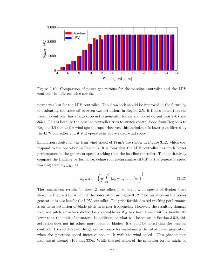
4 6 8 10 12 14 16 18 20 22 24 260
1,000
2,000
3,000
Wind speed [m/s]
Pow
er[k
W]
BaselineLPV
Figure 3.10: Comparison of power generations for the baseline controller and the LPVcontroller in different wine speeds.
power was lost for the LPV controller. This drawback should be improved in the future by
re-evaluating the trade-off between two actuations in Region 2.5. It is also noted that the
baseline controller has a large drop in the generator torque and power output near 280 s and
355 s. This is because the baseline controller tries to switch control loops from Region 3 to
Regions 2.5 due to the wind speed drops. However, this turbulence is lower pass filtered by
the LPV controller and it still operates in above rated wind speed.
Simulation results for the trim wind speed of 18 m/s are shown in Figure 3.12, which cor-
respond to the operation in Region 3. It is clear that the LPV controller has much better
performance on the generator speed tracking than the baseline controller. To quantitatively
compare the tracking performance, define root mean square (RMS) of the generator speed
tracking error ωg RMS as:
ωg RMS =
(1
T
∫ T
0|ωg − ωg rated|2dt
) 12
(3.12)
The comparison results for these 2 controllers in different wind speeds of Region 3 are
shown in Figure 3.13, which fit the observation in Figure 3.12. The variation on the power
generation is also less for the LPV controller. The price for this desired tracking performance
is an extra actuation of blade pitch in higher frequencies. However, the resulting damage
to blade pitch actuators should be acceptable as Wβ has been tuned with a bandwidth
lower than the limit of actuators. In addition, as what will be shown in Section 3.5.2, this
actuation does not introduce more loads on blades. It should be noted that the baseline
controller tries to decrease the generator torque for maintaining the rated power generation
when the generator speed increases too much with the wind speed. This phenomenon
happens at around 310 s and 330 s. While this actuation of the generator torque might be
45

200 220 240 260 280 300 320 340 360 380 400
11
12
13v
[m/s
]
200 220 240 260 280 300 320 340 360 380 4001,000
1,050
1,100
1,150
1,200
ωg
[RP
M]
BaselineLPV
200 220 240 260 280 300 320 340 360 380 40021
22
23
24
25
τg
[kN
m]
200 220 240 260 280 300 320 340 360 380 4002
4
6
8
10
β[d
eg]
200 220 240 260 280 300 320 340 360 380 4002,200
2,400
2,600
Time [s]
P[k
W]
Figure 3.11: Simulations for the baseline controller and the LPV controller at 12 m/s.
46

helpful to decrease variations of the power generation, it leads to the potential of instability
of the rotor dynamics as shown in Equation 2.2. In contrast, the LPV controller guarantees
the stability and provides better load reductions by moderately varying the generator torque
around the rated value. The range for this variation can be adjusted by tuning the weight
Wτ , according to constraints on the generator.
3.5.2 Damage Equivalent Load Analysis
This section provides the post analysis of simulation results on loads for a further comparison
between the two controllers. The metric for evaluating loads on the turbine is based on the
calculation of damage equivalent loads (DELs). The DELs show the equivalent fatigue
damage caused by the load on a specific component. The DELs can be calculated using the
MCrunch [73] which is also developed by NREL. Results of the DELs analysis for the two
controllers are shown in Figure 3.14 based on the data in 21 simulations as mentioned in
Section 3.5.1. Here, 5 different loads are considered which include the tower base bending
moments in fore-aft and side-to-side directions Mtfa and Mtss, high speed shaft torque τhss
and averaged blade flapwise and edgewise bending moments Mbfw and Mbss.
As shown in Figure 3.14, all loads generally increase with the wind speed, except for the
blade edgewise bending moment. The detailed check on this load shows that the vibration
of blades in the edgewise direction is dominated by the periodic motion of the rotation.
Therefore, collective pitch control has few effects on this load. It is also noted that the high
speed shaft torque reaches its maximum in Region 2.5. This makes sense as the turbine
still uses the generator torque as the main control input for power maximization in Region
2.5, where the wind speed is sufficient high to introduce large vibrations on the generator
torque.
Improvements for the LPV controller on load reduction are shown in Figure 3.15 by com-
paring to the baseline controller on DELs. It is seen in this figure that the load reduction
effect is not obvious in Region 2 for the LPV controller. This is because load reduction is
less critical in Region 2 and less emphasis has been put in the corresponding weight of wind
turbulence W(1)v . In Region 2.5, the LPV controller starts to show better load reduction
results than the baseline controller. However, there is a trade off between the blade flapwise
bending moment and the high speed shaft torque. As the high speed shaft torque is similar
to the generator torque, considering the lightly damped drive train torsion mode in the high
frequency, this observation reflects the balance of two actuations in Region 2.5. In Region
3, the LPV controller has much less DELs than the baseline controller. Specifically, there is
about 20 % decrease of the DEL on the high speed shaft torque. The improvement for the
blade flapwise bending moment is about 10 %. The load reductions on the tower fore-aft
47

200 220 240 260 280 300 320 340 360 380 400
16
18
20
22v
[m/s
]
200 220 240 260 280 300 320 340 360 380 400
1,100
1,150
1,200
ωg
[RP
M]
BaselineLPV
200 220 240 260 280 300 320 340 360 380 400
23.2
23.4
23.6
23.8
τg
[kN
m]
200 220 240 260 280 300 320 340 360 380 400
14
16
18
20
22
β[d
eg]
200 220 240 260 280 300 320 340 360 380 400
2,400
2,500
2,600
Time [s]
P[k
W]
Figure 3.12: Simulations for the baseline controller and the LPV controller at 18 m/s.
48
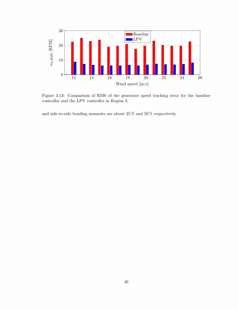
12 14 16 18 20 22 24 260
10
20
30
Wind speed [m/s]
ωg
RM
S[R
PM
]
BaselineLPV
Figure 3.13: Comparison of RMS of the generator speed tracking error for the baselinecontroller and the LPV controller in Region 3.
and side-to-side bending moments are about 25 % and 50 % respectively.
49

4 6 8 10 12 14 16 18 20 22 24 260
1
2
3τ
hss
4 6 8 10 12 14 16 18 20 22 24 260
500
1,000
1,500
Mb
fw
4 6 8 10 12 14 16 18 20 22 24 260
1,000
2,000
3,000
Mb
ew
4 6 8 10 12 14 16 18 20 22 24 260
0.5
1
·104
Mtf
a
4 6 8 10 12 14 16 18 20 22 24 260
2,000
4,000
6,000
v [m/s]
Mts
s
BaselineLPV
Figure 3.14: Damage equivalent loads (DELs) for the baseline controller and the LPVcontroller at different wind speeds.
50

4 6 8 10 12 14 16 18 20 22 24 26
−40
−20
0
20
40τ
hss
[%]
4 6 8 10 12 14 16 18 20 22 24 26
−20
0
20
Mb
fw[%
]
4 6 8 10 12 14 16 18 20 22 24 26−1
−0.5
0
0.5
1
Mb
ew[%
]
4 6 8 10 12 14 16 18 20 22 24 26−40
−20
0
Mtf
a[%
]
4 6 8 10 12 14 16 18 20 22 24 26
−50
0
v [m/s]
Mts
s[%
]
Figure 3.15: Improvements for the LPV controller on load reduction at different windspeeds.
51

Chapter 4
Robust Synthesis for LPV Systems
Using IQCs
4.1 Introduction
This chapter considers the robust synthesis problem for a class of uncertain linear parameter
varying (LPV) systems. The uncertain system is described as an interconnection of a nom-
inal (not-uncertain) LPV system and a block structured uncertainty. The state matrices of
the nominal system are assumed to have an arbitrary dependence on parameters, i.e. the
nominal part is a “gridded” LPV system. Such models arise naturally in many applications
via linearization of a nonlinear model around parameterized operating (trim) points. Spe-
cific examples of current interest include aeroelastic vehicles [74] and wind turbines [63,75].
The input/output behavior of the uncertainty is described by integral quadratic constraints
(IQCs) [19]. The use of IQCs is sufficiently general to describe “uncertain” components that
include nonlinearities, e.g. saturation, in addition to (parametric or dynamic) uncertainty.
The robust synthesis problem, formulated in Section 4.3.1, involves a search for a controller
that minimizes a closed-loop robust performance metric. This leads to a non-convex opti-
mization that involves a search for both the controller state matrices and the IQC analysis
variables. The proposed algorithm, given in Section 4.3.3, consists of a coordinate-wise
descent similar to the well-known DK-iteration [20,76] for µ synthesis. Specifically, the pro-
posed algorithm alternates between an LPV synthesis step and an IQC analysis step. The
synthesis step essentially relies on existing results for nominal (not) uncertain ”gridded”
LPV systems in [57,58]. The analysis step is performed using a matrix inequality condition
to bound the robust performance of the closed-loop uncertain LPV system (Section 4.4.1).
Both steps can be efficiently solved as semidefinite programs (SDPs). The effectiveness of
52

the proposed method is demonstrated on a simple numerical example in Section 4.5.
There are two main technical challenges in developing this algorithm. First, the nominal
LPV system does not have a valid frequency response interpretation and hence the robust-
ness analysis requires a time domain approach. Section 4.4.1 develops a matrix inequality
robustness analysis condition (Theorem 3) using (time domain) dissipation inequality tech-
niques. This result requires several technical lemmas to convert a conic combination of
many frequency domain IQCs into a single, equivalent time domain IQC. This analysis
condition is an extension of the worst-case gain condition in [77,78]. We note that there are
alternative robust stability conditions for time-varying systems based on the ν-gap metric
rather than dissipation inequalities [79]. These alternative robust stability conditions can
potentially be used to develop synthesis algorithms complementary to those developed here.
The second technical challenge is that an appropriate scaled system must be constructed
to link the analysis and synthesis steps. In particular, the single equivalent time domain
IQC from the analysis step must be combined with the nominal open-loop system to cre-
ate the scaled system. This construction, described in Section 4.4.2, is such that the next
synthesis step on the scaled plant yields a controller that improves the closed-loop robust
performance. These technical results are used to show the following main result in Sec-
tion 4.4.3: the robust performance metric is non-increasing at each iteration step and hence
the algorithm converges.
This chapter builds on many known results for both LPV systems and IQCs. A brief
review of these existing results is provided in Section 4.2. In addition, there are several
related robust synthesis results for LPV systems [68,80–83]. These existing robust synthesis
results are for the case where the state matrices of the nominal LPV system have a rational
dependence on the scheduling parameters. This rational (linear fractional) dependence on
the parameters is exploited in the algorithm development and leads to finite-dimensional
matrix inequalities for both the synthesis and analysis steps. In contrast, the algorithm in
this chapter is developed for the case where the state matrices of the nominal LPV system
have an arbitrary dependence on the parameters. As noted above, this enables applications
to systems, e.g. aeroelastic aircraft or wind turbines, for which arbitrary dependence on
scheduling parameters is a natural modeling framework. The drawback of this approach is
that it leads to parameter-dependent matrix inequalities for both the synthesis and analysis
steps. As a result, parameter gridding is required to obtained finite-dimensional matrix
inequality conditions. Finally, this chapter builds on a related conference paper submission
[84]. The conference paper only considered LTI uncertainty while this chapter considers
(possibly nonlinear) components whose input/output behavior are described by a general
class of dynamic IQCs.
53

4.2 Integral Quadratic Constraints
Integral quadratic constraints (IQCs) [19] provide a framework for robustness analysis build-
ing on work by Yakubovich [85]. The IQC specifies a constraint on the input-output signals
of the perturbation. The form of the constraint is such that it can be easily incorporat-
ed into tractable stability and performance analysis conditions. The following definitions
characterize the constraint in the frequency and time domain.
Definition 1. Let Π ∈ RL(nv+nw)×(nv+nw)∞ be a rational and uniformly bounded function
of jω. Two signals v ∈ Lnv2 [0,∞) and w ∈ Lnw2 [0,∞) satisfy the frequency domain IQC
defined by the multiplier Π if∫ ∞−∞
[V (jω)
W (jω)
]∗Π(jω)
[V (jω)
W (jω)
]dω ≥ 0 (4.1)
where V and W are Fourier transforms of v and w. A bounded, causal operator ∆ :
Lnv2e [0,∞) → Lnw2e [0,∞) satisfies the frequency domain IQC defined by Π if Equation 4.1
holds for all v ∈ Lnv2 [0,∞) and w = ∆(v).
Definition 2. Let Ψ be a stable LTI system, i.e. Ψ ∈ RHnz×(nv+nw)∞ , and M = MT ∈
Rnz×nz . Two signals v ∈ Lnv2e [0,∞) and w ∈ Lnw2e [0,∞) satisfy the time domain IQC defined
by the multiplier Ψ and matrix M if the following inequality holds for all T ≥ 0∫ T
0zT (t)Mz(t) dt ≥ 0 (4.2)
where z is the output of Ψ driven by inputs (v, w) with zero initial conditions. A bounded,
causal operator ∆ : Lnv2e [0,∞)→ Lnw2e [0,∞) satisfies the time domain IQC defined by (Ψ,M)
if Inequality 4.2 holds for all v ∈ Lnv2e [0,∞), w = ∆(v) and T ≥ 0.
IQCs can be used to model a variety of nonlinearities and uncertainties. In particular, [19]
provides a library of frequency domain IQC multipliers that are satisfied by many important
system components, e.g. saturation, time delay, and norm bounded uncertainty. Figure 4.1
provides a graphical interpretation for the time domain IQC. The input and output signals
of ∆ are filtered through Ψ. If ∆ satisfies the time domain IQC defined by Ψ then the
filtered signal z satisfies the constraint in Equation 4.2 for any finite-horizon T ≥ 0.
A precise connection between the frequency and time domain IQC formulations is im-
portant for the robust synthesis algorithm described in this chapter. Assume ∆ satis-
fies the time domain IQC defined by (Ψ,M). Taking T → ∞ in Equation 4.2 yields
54

v - ∆w-
-
- Ψz-
Figure 4.1: Graphical interpretation of the IQC.
∫∞0 z(t)TMz(t) dt ≥ 0. By Parseval’s theorem [20], this is equivalent to the frequency do-
main constraint∫∞−∞ Z(jω)∗MZ(jω) dω ≥ 0 where Z(jω) = Ψ(jω)
[V (jω)
W (jω)
]. Thus if ∆
satisfies the time domain IQC defined by (Ψ,M) then it satisfies the frequency domain IQC
defined by Π = Ψ∼MΨ.
The reverse implication is more technical and fails to hold in general. Specifically, assume ∆
satisfies the frequency domain IQC defined by the multiplier Π. Any rational multiplier Π
can be factorized as Π = Ψ∼MΨ where Ψ ∈ RHnz×(nv+nw)∞ is stable and M = MT ∈ Rnz×nz .
Such factorizations are not unique but can be computed using state-space calculations
[86–88]. One specific numerical construction is given by Lemma 4 in Appendix A. Substitute
the factorization for Π into the frequency domain IQC (Equation 4.1) and apply Parseval’s
theorem [20] to convert to a time domain constraint. This yields∫∞
0 z(t)TMz(t) dt ≥ 0
where z is the output of Ψ driven by v and w = ∆(v) with zero initial conditions. This
time domain constraint holds, in general, only over infinite horizons and only for finite-
norm input signals v ∈ Lnv2 [0,∞). However, the time domain IQC (Definition 2) requires
the integral inequality to hold over all finite times T ≥ 0 and for all extended-space input
signals v ∈ Lnv2e [0,∞). A time domain IQC as in Definition 2 is referred to as a hard IQC
in [19]. In contrast, factorizations for which the time domain constraint holds only for
T =∞ are called soft IQCs. This distinction is important because the dissipation theorems
specified later for robustness analysis require the use of hard IQCs.1 Lemmas 5 and 6
in Appendix A provide a specific ”hard” factorization (Ψ,M) that can be constructed
under additional assumptions on the frequency domain multiplier Π. To summarize these
lemmas, let Π = Π∼ ∈ RL(nv+nw)×(nv+nw)∞ be partitioned as
[Π11 Π12Π∼12 Π22
]where Π11 ∈ RLnv×nv∞
and Π22 ∈ RLnw×nw∞ . If Π11(jω) > 0 and Π22(jω) < 0 ∀ω ∈ R ∪ {∞}, then Π has a
hard factorization (Ψ,M) that yields a time domain IQC (Definition 2). (Ψ,M) can be
constructed from the stabilizing solution to an Algebraic Riccati Equation (ARE) and is
called a J-spectral factorization of Π.
LPV systems do not have a valid frequency response interpretation. Hence existing condi-
tions for robust analysis of gridded LPV systems [77,78] rely on the use of valid time domain
1The terms “complete” and “conditional” IQCs in [89] are generalizations of hard and soft IQCs. Thehard/soft terminology will be used here.
55

(hard) IQCs. Section 4.4.1 generalizes these existing results to handle factorizations (Ψ,M)
that are not necessarily hard. Moreover, analysis conditions for a worst-case gain metric are
provided in [77,78]. Here, analysis conditions are derived for a robust performance metric.
Definitions of these two metrics and their difference will be introduced in Section 4.3.1.
4.3 Robust Synthesis Algorithm
4.3.1 Problem Formulation
Consider the robust synthesis problem for the uncertain LPV system as shown in Figure 4.2.
The uncertain LPV system is described by the interconnection of an open loop LPV system
Gρ, a perturbation ∆, and an LPV controller Kρ. A state-space realization for Gρ is given
by: xG
v
e
y
=
A(ρ) Bw(ρ) Bd(ρ) Bu(ρ)
Cv(ρ) Dvw(ρ) Dvd(ρ) Dvu(ρ)
Ce(ρ) Dew(ρ) Ded(ρ) Deu(ρ)
Cy(ρ) Dyw(ρ) Dyd(ρ) Dyu(ρ)
xG
w
d
u
(4.3)
where xG ∈ RnG , w ∈ Rnw , d ∈ Rnd , u ∈ Rnu , v ∈ Rnv , e ∈ Rne and y ∈ Rny . The following
assumptions are made regarding Gρ and ∆:
Assumption 1. Gρ is quadratically stabilizable from u and quadratically detectable from y
as defined in Chapter 1 of [57].
Assumption 2. The perturbation is a bounded, causal operator ∆ : Lnv2e [0,∞)→ Lnw2e [0,∞)
that satisfies a collection of IQCs defined by {Πk}Nk=1 ⊂ RL(nv+nw)×(nv+nw)∞ in the frequency
domain.
Assumption 3. Partition the frequency domain multipliers {Πk}Nk=1 as[
Πk,11 Πk,12Π∼k,12 Πk,22
]where
Πk,11 is nv×nv. Each frequency domain multiplier satisfies Πk,11(jω) ≥ 0 and Πk,22(jω) ≤ 0
∀ω ∈ R ∪ {∞}.
Assumption 4. The perturbation has been normalized to satisfy ‖∆‖ ≤ 1 and the first IQC
is defined by the multiplier Π1 :=[Inv 00 −Inw
].
The first assumption ensures that there is a controller Kρ from y to u that stabilizes the
(nominal) open loop interconnection of Gρ and Kρ. This open loop interconnected system
is a lower LFT, denoted Fl(Gρ,Kρ). The IQCs in the second assumption are used to bound
the input-output behavior of the perturbation ∆. This formulation can handle systems
where ∆ has block diagonal structure including static nonlinearities (e.g. saturations) and
56

Gρ d�e �
∆
v
-
w
�
Kρ
y
-
u
�
Figure 4.2: Interconnection for LPV robust synthesis.
infinite dimensional operators (e.g. time delays) in addition to true system uncertainties.
The term “uncertainty” is used for simplicity when referring to the perturbation ∆. The
notation ∆(Π1, . . . ,ΠN ) will be used to denote the set of bounded, causal operators ∆ that
satisfy all frequency domain IQCs defined by {Πk}Nk=1.
The third and fourth assumptions are used to simplify the algorithm. Assumption 3 only re-
quires the multipliers satisfy non-strict definiteness conditions Πk,11 ≥ 0 and Πk,22 ≤ 0. This
is sufficiently general to cover most typical frequency domain multipliers used in IQC anal-
ysis. In fact, all frequency domain multipliers listed in [19] satisfy Πk,11 ≥ 0 and Πk,22 ≤ 0
except those for certain sector bounded nonlinearities and polytopic uncertainties which fail
to contain the zero operator ∆ = 0. Finally, note that the individual multiplier Πk need not
satisfy the strict definiteness conditions Πk,11 > 0 and Πk,22 < 0 given in Lemma 5 for the
existence of a J-spectral factorization. However, Assumptions 3 and 4 are sufficient to en-
sure that a “combined” multiplier that appears in the proposed robust synthesis algorithm
satisfies the strict definiteness conditions and thus has a J-spectral factorization. Specifi-
cally, the “combined” multiplier described below will be formed (with an additional scaling
neglected here) as: Πλ :=∑N
k=1 λkΠk. The coefficients will be constrained to satisfy λ1 > 0
and λk ≥ 0 for k = 2, . . . N . Assumptions 3 and 4 along with these constraints on λ are
sufficient to ensure that the combined multiplier satisfies the strict definiteness conditions
Πλ,11 > 0 and Πλ,22 < 0 given in Lemma 5. Other parameterizations of the IQC multiplier
are possible. For example, [90] uses the form Πλ := Ψ∗M(λ)Ψ where Ψ is a given stable
filter (not necessarily square) and M is an affine matrix function of λ. The robust synthesis
algorithm proposed here can be generalized to handle alternative parameterizations as long
as the conditions Πλ,11 > 0 and Πλ,22 < 0 can be enforced as a convex constraint on λ.
To simplify notation, define Hρ := Fl(Gρ,Kρ). The uncertain LPV system in Figure 4.2
can therefore be expressed as an upper LFT, denoted Fu(Hρ,∆). A natural performance
57

metric for the uncertain LPV system is the worst-case gain:
sup∆∈∆(Π1,...,ΠN )
‖Fu(Hρ,∆)‖ (4.4)
This is the largest induced L2 gain of the uncertain LPV system over all uncertainties
consistent with the specified IQCs. This metric has been widely used for robustness analysis
[77,78,91]. Note that the worst-case gain is only finite (< +∞) if the controller Kρ robustly
stabilizes the plant over any uncertainty ∆ ∈ ∆. Hence the use of worst-case gain for
robust synthesis requires an initial controller that achieves robust stability. It is possible
to construct a two-stage synthesis algorithm that in the first stage attempts to design a
robustly stabilizing controller and in the second stage attempts to minimize the worst-case
gain. The first stage requires a way to measure the “robustness” of the controller relative to
the uncertainty set ∆. A scaled uncertainty set can serve this purpose. Specifically, define
Sb as the scaling matrix[bInv 0
0 Inw
]. Let ∆b(Π1, . . . ,ΠN ) denote the set of bounded, causal
operators ∆ that satisfy the frequency domain IQCs defined by SbΠkSb for k = 1, . . . , N .
For the scaled set, if b2 ≥ b1 then ∆b2 ⊇ ∆b1 .2 This inclusion means that stability with
respect to a scaled uncertainty set ∆b defined by b provides a useful robustness metric,
i.e. larger values of b indicate more robustness. For many multipliers this scaling has
a simple interpretation. For example, Π :=[
1 00 −1
]defines norm bounded uncertainty
‖∆‖ ≤ 1. For this multiplier the scaled set ∆b(Π) corresponds to SbΠSb =[b2 00 −1
]and
defines uncertainty ‖∆‖ ≤ b. In some cases the interpretation is not as intuitive. For
example, Zames-Falb multipliers can be used to describe an uncertainty set ∆ that contains
monotonic nonlinearities such as the saturation. The scaled uncertainty set does not have
an easy interpretation for such IQC multipliers. In these cases we can simply state that if a
controller achieves robust stability with b ≥ 1 then it achieves robust stability with respect
to the unscaled set ∆.
The two-stage algorithm proposed above would use both a robust stability and worst-
case gain metric. It is more convenient to combine these stages into a single algorithm.
Specifically, it is standard, e.g. in DK synthesis, to instead use a robust performance metric
that simultaneously scales both the uncertainty level and the system gain. This metric,
formally defined below, is used for the robust synthesis algorithm in this chapter. The
definition of robust performance uses the notion of a scaled uncertainty set discussed above.
Definition 3. The system Hρ achieves robust performance of level γ with respect to the
2A sketch of the proof is given. Assume Π11(jω) ≥ 0 and Π22(jω) ≤ 0 ∀ω ∈ R ∪ {∞}. LetV and W be Fourier transforms of two signals in L2. Define a function f : R>0 → R by f(b) :=∫∞−∞
[bV (jω)
W (jω)
]∗Π(jω)
[bV (jω)
W (jω)
]dω. It can be shown that if f(b1) ≥ 0, then f ′(b) ≥ 0 ∀b ≥ b1. This can
be used to show that if (V ,W ) satisfy the scaled IQC defined by Sb1ΠSb1 then (V ,W ) satisfy the scaled IQCfor any b2 ≥ b1.
58

uncertainty described by {Πk}Nk=1 if
sup∆∈∆1/γ(Π1,...,ΠN )
‖Fu(Hρ,∆)‖ ≤ γ (4.5)
Let r∆(Π1,...,ΠN )[Hρ] denote the smallest level of robust performance achievable by Hρ.
Hρ achieves robust performance of level γ if the worst-case induced L2 gain from d to e
is ≤ γ over all uncertainties in the scaled set ∆1/γ(Π1, . . . ,ΠN ). For decreasing levels of
robust performance, the gain decreases and the bound of the tolerable uncertainty increases.
The robust performance level for the uncertain system with known nominal plant Hρ can
be analyzed using convex optimization as described in Section 4.4.1.
The objective of the robust synthesis problem is to synthesize an LPV controller Kρ with the
form in Equation 3.6 that stabilizes the open-loop model Gρ and minimizes the closed-loop
robust performance. Thus the synthesis problem is:
infKρ stabilizing
r∆(Π1,...,ΠN) [Fl(Gρ,Kρ)] (4.6)
It is typical to scale the performance weights to achieve a robust performance metric near
1. This ensures that the synthesized controller robustly stabilizes the modeled (unscaled)
uncertainty.
4.3.2 DK Synthesis
This section briefly reviews the standard DK synthesis algorithm [20, 76]. The objective is
to clarify the notation presented thus far and to provide a basis for comparison with the
proposed algorithm. In DK synthesis the nominal plant G is LTI and the uncertainty ∆
is LTI and unit norm bounded. The robust synthesis problem involves the search for an
LTI controller K and robustness analysis scalings D (called D-scales). The problem is non-
convex, in general, and DK synthesis employs a coordinate-wise iteration. Specifically, the
algorithm iterates between a controller synthesis step (K-step) and a robustness analysis
step (D-step). The synthesis step involves the design of an H∞ controller K on a nom-
inal (not-uncertain) scaled system. The analysis step involves the search for a frequency
domain scaling D to assess the robust performance of the closed-loop H := Fl(G,K). The
coordinate-wise iteration for DK synthesis does not, in general, converge to a local (nor
global) optima. However it has the advantage that each of the decoupled synthesis and
analysis steps is a convex optimization.
The main technical result for DK synthesis is that the iteration is well posed at each
59

step and the robust performance is (in theory) non-increasing. This result is based on the
construction of a scaled system that links the analysis and synthesis steps. The scaled system
used in the K-step is DGD−1 where D is the scaling from the analysis step. The main loop
theorem [20] establishes the equivalence between robust performance of the (uncertain)
closed-loop Fu(H,∆) and the induced L2 performance of the (not-uncertain) scaled system
Fl(DGD−1,K). If the synthesis problem includes mixed (real and complex) uncertainty
then the construction of an appropriate scaled system is more subtle. For example, the
DGK synthesis algorithm [92,93] uses a specific factorization of the D/G scalings to prove
that the robust performance monotonically decreases. One of the major technical results
given below leads to the construction of an appropriate scaled system for the robust LPV
synthesis with general IQCs.
Finally, we briefly connect the notation used in standard DK synthesis with that introduced
here for the robust LPV synthesis problem. The uncertainty in DK synthesis is, in general,
block structured but for simplicity this discussion assumes ∆ is SISO (no structure). If
‖∆‖∞ ≤ 1 then ∆ satisfies the frequency domain IQC defined by Π =[α 00 −α
]for any SISO,
LTI system α such that α(jω) = α(jω)∗ > 0 ∀ω ∈ R ∪ {∞}. Moreover, if ‖∆‖∞ ≤ 1γ
then ∆ satisfies the frequency domain IQC defined by the scaled multiplier S1/γΠS1/γ .
The condition α > 0 ensures that α has a spectral factorization α = d∼d where d is the
scaling/multiplier that appears in DK synthesis. In this case, Ψ =[d 00 d
]and M =
[1 00 −1
]defines a J-spectral factorization of Π. The D-step in DK synthesis is typically implemented
by solving for D-scales on a frequency grid and then fitting the result with a rational transfer
function. Here, the scalings will be restricted to a finite, linear combination of user selected
basis functions. In particular, the definition of robust performance (Definition 3) requires
a finite number N of (fixed) multipliers {Πk} to be specified. In the context of this DK
synthesis example, this corresponds to the selection of N scalings {αk}. The proposed
algorithm given below will search for the best linear combination of these scalings.
4.3.3 Algorithm Description
This section gives a high-level overview of the proposed LPV robust synthesis algorithm.
Technical details regarding the algorithm are then given in Section 4.4. As in DK syn-
thesis, the robust LPV synthesis is, in general, non-convex. In particular, Theorem 3 in
Section 4.4.1 provides a linear matrix inequality (LMI) formulation for robust performance.
Applying this result for synthesis leads to a matrix inequality condition that is bilinear in
the state matrices for the controller Kρ and the analysis variables consisting of a storage
matrix P ≥ 0 and IQC coefficients {λk}Nk=1. A standard coordinate-wise approach is used
to decouple the design into a nominal controller synthesis step (for Kρ) and a robust per-
formance analysis step (for P and λ). The technical results in Section 4.4 are used to link
60

these steps.
The detailed steps of the algorithm including the initialization and termination conditions
are described in Algorithm 1. This algorithm is briefly described to provide a roadmap for
the technical results in the following section. The algorithm initialization (Step 2) computes
a factorization for each IQC multiplier. Any stable factorization of the Πk may be used in
and the construction in Lemma 4 of Appendix A is just one possibility. As noted above,
a J-spectral factorization need not exist for the individual multipliers Πk and hence the
factorization need not be “hard”. The main steps of the algorithm involve a synthesis step
(Step 8), analysis step (Step 9), and the construction of a scaled-system Gsclρ that links these
steps (Steps 5-7). The synthesis ste is a standard (nominal) LPV synthesis on the scaled
system. It uses the algorithm in [57,58] and summarized by Theorem 2 in Section 3.2. The
analysis step is a parameterized matrix inequality condition (Theorem 3 in Section 4.4.1)
that involves a storage function matrix P , analysis vector λ, and robust performance bound
γ. The bound γ enters bilinearly in the matrix inequality and hence this step requires
bisection to find the minimum feasible value of γ. This step can be interpreted as a search
over linear combinations of the scaled IQCs to form a single combined IQC multiplier (Step
6). The technical condition λ1(i) > 0 in Step 9 is used to ensure that the combined IQC
multiplier in Step 6 has a J-spectral factorization. In particular, Assumption 3 along with
λ ∈ R≥0 implies that Πλ satisfies the non-strict conditions Πλ,11 ≥ 0 and Πλ,22 ≤ 0.
Assumption 4 gives Π1 :=[I 00 −I
]so that λ1(i) > 0 ensures that the strict conditions
Πλ,11 > 0 and Πλ,22 < 0 are satisfied. Hence the combined multiplier has a J-spectral
factorization by Lemma 5. Finally, the analysis and synthesis steps are linked by the
construction of a particular scaled system (Step 7). The construction of the scaled system
is described further in Section 4.4.2. The algorithm can be easily modified to incorporate
other termination criteria in Step 10, e.g. maximum number of iterations and/or relative
stopping tolerances.
As noted above, the LPV robust synthesis problem inherits the non-convexity of DK syn-
thesis. The proposed coordinate-wise iteration will not, in general, converge to a local (nor
global) optima. However, it is a pragmatic approach that decouples the synthesis and analy-
sis steps into convex optimizations. The main technical result (Theorem 4 in Section 4.4.3)
is that the algorithm iteration is well posed at each step and the robust performance is
non-increasing. This is similar to the convergent property of the DK synthesis.
61

Gρu�y �d�e �
Ψ†λ
v
-wλ - vλ-
w
�
Figure 4.3: LFT interconnection of Scaled System, Gsclρ .
4.4 Technical Details
4.4.1 Robust Performance Condition
This section derives a matrix inequality condition to bound the robust performance for
an uncertain LPV system. The uncertain LPV system is specified by the interconnection
Fu(Hρ,∆). The main technical issue is that the uncertainty ∆ is described by IQCs {Π}Nk=1
in the frequency domain but the nominal system Hρ is LPV and does not have a valid
frequency domain interpretation. The approach given here combines the frequency domain
IQCs and converts it to a single, equivalent time domain IQC. The steps in this section
alternate between various conditions involving the frequency domain IQCs and the single
time domain IQC. This leads to the main technical result (Theorem 3) which involves a
dissipation inequality characterization for robust performance.
The nominal LPV system Hρ has the following state-space realization:xHve
=
A(ρ) Bw(ρ) Bd(ρ)
Cv(ρ) Dvw(ρ) Dvd(ρ)
Ce(ρ) Dew(ρ) Ded(ρ)
xHwd
(4.7)
where xH ∈ RnH , w ∈ Rnw , d ∈ Rnd , v ∈ Rnv and e ∈ Rne . The uncertainty ∆ is assumed
to satisfy multiple frequency domain IQCs defined by {Πk}Nk=1 under Assumptions 2, 3
and 4 in Section 4.3.1. Construct a factorization for each Πk as (Ψk,Mk) where Ψk is
stable, e.g. using the basic method described by Lemma 4 in Appendix A. The special
J-spectral factorization is not required at this point. In fact, the individual Πk need not
satisfy the special sign-definiteness conditions specified in Lemma 5 for constructing a J-
spectral factorization. Moreover, it should be emphasized that the factorization (Ψk,Mk)
need not specify a valid time domain IQC as given by Definition 2.
The factorizations {(Ψk,Mk)}Nk=1 are constructed for the multipliers {Πk}Nk=1 that define
the normalized uncertainty set ∆(Π1, . . . ,ΠN ). Recall that the definition of robust perfor-
mance involves the scaled uncertainty set ∆1/γ(Π1, . . . ,ΠN ). This corresponds to the use of
the scaled (frequency domain) multipliers S1/γΠkS1/γ (k = 1, . . . , N). Thus a factorization
62

for each scaled multiplier is given by (ΨkS1/γ ,Mk). Let zk denote the output of the scaled
system ΨkS1/γ driven by the input/output signals (v, w) of ∆ assuming zero initial condi-
tions. Then all {ΨkS1/γ}Nk=1 can be aggregated into a single system denoted Ψ1/γ with the
following (minimal) state-space realization:
[xψ(t)
zk(t)
]=
[A γ−1Bv Bw
Czk γ−1Dzkv Dzkw
]xψ(t)
v(t)
w(t)
(k = 1, . . . , N) (4.8)
Equation 4.8 uses an abbreviated notation to denote that the outputs of Ψ1/γ are [zT1 , . . . zTN ]T .
Note that the scaling matrix S1/γ :=[γ−1Inv 0
0 Inw
]only modifies the state matrices of Ψ1/γ
associated with the v input, i.e. it only scales the Bv and Dzkv matrices.
The robust performance analysis is based on the interconnection shown in Figure 4.4 with
∆ ∈ ∆1/γ(Π1, . . . ,ΠN ). The dynamics of this analysis interconnection are described by
w = ∆(v) and the extended system of Hρ and Ψ1/γ :
xzke
=
A(ρ) Bw(ρ) Bd(ρ)
Czk(ρ) Dzkw(ρ) Dzkd(ρ)
Ce(ρ) Dew(ρ) Ded(ρ)
xwd
(k = 1, . . . , N) (4.9)
where the state vector is x = [xH ;xψ] ∈ RnH+nψ with xH and xψ being the state vectors of
the LPV system Hρ and the filter Ψ1/γ , respectively. The state matrices for the extended
system can be expressed in terms of the state matrices for Hρ (Equation 4.7) and Ψ1/γ
(Equation 4.8). Appendix B provides one realization. Note that the state matrices of the
extended system depend on the robust performance level γ. However this dependence on
γ is not explicitly denoted. The uncertainty ∆ is shown in the dashed box of Figure 4.4
to signify that the analysis condition given below is specified only in terms of the extended
system of Hρ and Ψ1/γ . This effectively overbounds the precise relation w = ∆(v) with the
IQCs satisfied by ∆.
Hρd�e �
∆
v
-
w
�
-
-Ψ1/γ
zk-
Figure 4.4: Uncertain LPV system extended to include filter Ψ1/γ .
63

The robust performance analysis condition (given below) relies on a connection between
Ψ1/γ and a combined multiplier Πλ :=∑N
k=1 λkS1/γΠkS1/γ defined by scalars {λk}Nk=1 with
conditions that λ1 ∈ R>0 and λk ∈ R≥0 (k = 2, . . . , N). This combined multiplier can be
expressed in terms of the state-space realization of Ψ1/γ (Equation 4.8) as:
Πλ =[
(−sI−A)−1BI
]T [ Qλ SλSTλ Rλ
] [(sI−A)−1B
I
](4.10)
where
B :=[γ−1Bv Bw
](4.11)[
Qλ Sλ
STλ Rλ
]:=
N∑k=1
λk
CTzkγ−1DTzkv
DTzkw
Mk [ Czk γ−1Dzkv Dzkw ] (4.12)
Note that conditions on {λk}Nk=1 along with Assumptions 3 and 4 imply that (Πλ)11(jω) > 0
and (Πλ)22(jω) < 0 ∀ω ∈ R∪{+∞}. Therefore Πλ has a J-spectral factorization (Lemma 5).
This factorization is constructed from the stabilizing solution X to the ARE in Equation A.2
with (A, B, Qλ, Sλ, Rλ). Without loss of generality, the J-spectral factorization can be
rescaled as (Ψλ,Mλ) where the constant matrix is Mλ :=[γ−2I 0
0 −I
]. Specifically, Let (Ψ,M)
be a J-spectral factorization of Πλ with M :=[I 00 −I
]. Then (Ψλ,Mλ) := (SγΨ, S1/γMS1/γ)
is another factorization of Πλ with the constant matrix given by S1/γMS1/γ =[γ−2I 0
0 −I
].
In addition, the properties of a J-spectral factorization given in Lemma 6 carry over for this
rescaled factorization. This rescaling will be important for the construction of the scaled
plant in the synthesis step of our proposed algorithm (described in Section 4.4.2). The
rescaled filter Ψλ only has one output and has a state-space realization of the form:
[xψ(t)
zλ(t)
]=
[A γ−1Bv Bw
Czλ Dzλv Dzλw
]xψ(t)
v(t)
w(t)
(4.13)
This rescaled system Ψλ has the same state matrix A and input matrix [γ−1Bv, Bw] as the
original filter Ψ1/γ . Only the output and feedthrough matrices of Ψλ are different from
those in Ψ1/γ . Finally, an extended system of Hρ and Ψλ can be formed yielding:
xzλe
=
A(ρ) Bw(ρ) Bd(ρ)
Czλ(ρ) Dzλw(ρ) Dzλd(ρ)
Ce(ρ) Dew(ρ) Ded(ρ)
xwd
(4.14)
The state matrices for this extended system can be expressed in terms of the state ma-
trices for Hρ (Equation 4.7) and Ψλ (Equation 4.13). Only the output and feedthrough
64

matrices associated with zλ in this alternative extended system differ from those given in
Equation 4.9. Appendix B provides explicit formulae for Czλ , Dzλw, and Dzλd. Again, the
dependence on γ is not made explicit in this notation for the alternative extended system.
The robust performance condition relies on a technical lemma regarding matrix inequalities
associated with the two extended systems presented thus far. Specifically, the extended
system of Hρ and Ψ1/γ (Equation 4.9) can be used to define the following parameterized
matrix inequality involving multiple IQCs:[PA+ATP PBw PBdBTwP 0 0
BTd P 0 −I
]+
N∑k=1
λk
CTzkDTzkwDTzkd
Mk [ Czk Dzkw Dzkd ] +1
γ2
[CTeDTewDTed
][ Ce Dew Ded ] < 0
(4.15)
This matrix inequality is parameterized by ρ ∈ P through the dependence of the extended
system state matrices on the parameter. Similarly, the extended system of Hρ and Ψλ (E-
quation 4.14) can be used to define the following parameterized matrix inequality involving
the single, rescaled J-spectral factorization:[PA+AT P PBw PBdBTwP 0 0
BTd P 0 −I
]+
CTzλDTzλwDTzλd
Mλ [ Czλ Dzλw Dzλd ] +1
γ2
[CTeDTewDTed
][ Ce Dew Ded ] < 0 (4.16)
The technical result regarding these two matrix inequalities is formally stated in the next
Lemma.
Lemma 1. Let {Πk}Nk=1 ⊂ RL(nv+nw)×(nv+nw)∞ , γ > 0, and {λk}Nk=1 be givenwhere {Πk}Nk=1
satisfies Assumptions 3 and 4, λ1 ∈ R>0 and λk ∈ R≥0 (k = 2, . . . , N). Let each Πk
have a factorization (Ψk,Mk) where Ψk is stable. Define Πλ :=∑N
k=1 λkS1/γΠkS1/γ. Thus
(Πλ)11(jω) > 0 and (Πλ)22(jω) < 0 ∀ω ∈ R∪{+∞} and hence Πλ has a rescaled J-spectral
factorization (Ψλ,Mλ) as defined above. Let X denote the corresponding stabilizing solution
to the ARE (Equation A.2) with (A, B, Qλ, Sλ, Rλ). Finally, assume the nominal system
Hρ is stable.
Then, using the extended system notation defined above, the symmetric matrix P = P T
satisfies Equation 4.15 for all ρ ∈ P if and only if P := P+[
0 00 X
]≥ 0 satisfies Equation 4.16
for all ρ ∈ P.
Proof. See Appendix C.
This technical lemma is used to prove the following main result.
65

Theorem 3. Assume Fu(Hρ,∆) is well posed for all ∆ ∈ ∆1/γ(Π1, . . . ,ΠN ). Then Hρ
achieves robust performance of level γ if there exists a matrix P = P T ∈ R(nH+nψ)×(nH+nψ)
and scalars {λk}Nk=1 such that:
(i) (P, λ, γ) satisfy the parameterized matrix inequality in Equation 4.15 for all ρ ∈ P
(ii) λ1 ∈ R>0 and λk ∈ R≥0 (k = 2, . . . , N).
Proof. As described above, condition (ii) along with Assumptions 3 and 4 are sufficien-
t to ensure the combined multiplier Πλ :=∑N
k=1 λkS1/γΠkS1/γ satisfies (Πλ)11(jω) > 0
and (Πλ)22(jω) < 0 ∀ω ∈ R ∪ {+∞}. Hence Πλ has a rescaled J-spectral factorization
(Ψλ,Mλ). Define P := P +[
0 00 X
]≥ 0 where X is the stabilizing ARE solution used to con-
struct this factorization. By Lemma 1, P satisfies the parameterized matrix in equality in
Equation 4.16. The remainder of the proof is based on dissipation theory using the storage
function V : RnH+nψ → R+ defined as V (x) := xT P x. Left and right multiply Equation
4.16 by [xT , wT , dT ] and [xT , wT , dT ]T to show that V satisfies the dissipation inequality:
V (t) + zTλ (t)Mλzλ(t) ≤ d(t)Td(t)− γ−2e(t)T e(t) (4.17)
Append Ψλ to the (v, w) channels of the uncertain system Fu(Hρ,∆). This corresponds to
the interconnection shown in Figure 4.4 except with Ψλ replacing Ψ1/γ . Let (x,w, d, z, e) the
solution of this interconnection for some ∆ ∈ ∆1/γ(Π1, . . . ,ΠN ), disturbance d ∈ Lnd2 , ad-
missible trajectory ρ ∈ T , and zero initial conditions. Integrating the dissipation inequality
(4.17) along this solution from t = 0 to t = T yields:
V (x(T )) +
∫ T
0zλ(t)TMλzλ(t) dt+
1
γ2
∫ T
0e(t)T e(t) dt ≤
∫ T
0d(t)Td(t) dt (4.18)
It follows from λk ≥ 0 that ∆ ∈ ∆(Πλ). In addition, the rescaled J-spectral factorization
(Ψλ,Mλ) is a hard factorization of Πλ by Lemma 6. Therefore, (Ψλ,Mλ) is a valid time
domain IQC for ∆. Apply this time domain IQC along with P ≥ 0 to Equation 4.18 to
conclude that ‖e‖ ≤ γ‖d‖. Hence Hρ achieves RP of level γ.
The parameterized matrix inequality (Equation 4.15) in condition (i) of Theorem 3 involves
N IQCs. Note that left/right multiplying Equation 4.15 by [xT , wT , dT ] and [xT , wT , dT ]T
does not yield a true dissipation inequality for two reasons. First, (Ψk,Mk) does not need
to be a hard factorization and hence not a valid time domain IQC by Definition 2. Second,
the matrix P need not be positive definite and thus does not necessarily define a valid
storage function. The technical result in Lemma 1 addresses both issues. It converts the
original problem in an alternative form (equation 4.16) involving only a single, valid time
66

domain IQC. The alternative form involves P = P +[
0 00 X
]≥ 0 which defines a valid storage
function. The term X, which is the stabilizing solution of the ARE used to construct a
hard factorization, can be interpreted as additional energy. Finally, it is important to recall
that soft IQCs only hold, in general, over infinite time horizons and they require the signals
(v, w) to be in L2. Hence soft IQCs cannot be used in the dissipation inequality proof since
we do not know, a priori, that (v, w) are in L2. On the other hand, hard IQCs hold over
all finite time horizons and for all signals (v, w) in the extended space L2e. Hence a hard
factorization of Πλ is needed.
The conditions in Theorem 3 are sufficient to prove that the uncertain system satisfies a
certain level of robust performance (Definition 3). This ensures that ‖Fu(Hρ,∆)‖ ≤ γ for
all uncertainty ∆ ∈∆1/γ . This is a (finite-gain) input-output stability result, i.e. the gain
from input to output is less than γ < ∞, that appears frequently in literature, e.g. [94].
In fact, feasibility of the parameterized LMI in Equation 4.16 is sufficient to prove a type
of internal stability. In particular, the arguments in [95] (Proposition 1.2 and its proof)
demonstrate that the extended state x converges asymptotically to zero from any initial
condition and for any disturbance input d ∈ Lnd2 . In general, exponential convergence of
the extended state x does not hold and no conclusions regarding the “internal” state of ∆
can be made.
4.4.2 Scaled System
This section constructs a specific scaled system that will be used to link the analysis and
synthesis steps in our robust (IQC) synthesis algorithm. Consider the uncertain system
Fu(Hρ,∆). Theorem 3 provides a sufficient condition to ensure that Hρ achieves robust
performance of level γ. The proof involves a rescaled J-spectral factorization (Ψλ,Mλ). In
particular, robust performance is shown via a dissipation inequality (Equation 4.17) defined
for the extended system of Hρ and Ψλ. Recall that the J-spectral factorization was rescaled
so that Mλ :=[γ−2I 0
0 −I
]. Thus partitioning zλ := [ vλwλ ] simplifies the dissipation inequality
to
V (t) ≤(d(t)Td(t)− γ−2e(t)T e(t)
)+(wλ(t)Twλ(t)− γ−2vλ(t)T vλ(t)
)(4.19)
The form of this dissipation inequality implies a connection to nominal induced L2 gain
performance. Note that Theorem 1 in Section 3.2 provides a sufficient condition to upper
bound the induced L2 gain of an LPV system. The proof for this nominal performance
condition uses a dissipation inequality (Equation 3.4) that is similar to Equation 4.19.
In particular, Equation 4.19 has the form of a dissipation inequality used to prove a (not-
uncertain) LPV system with inputs (wλ, d) and outputs (vλ, e) has induced gain ≤ γ. Based
67

on this insight, a scaled system will be constructed with these inputs and outputs. First,
rewrite the extended system of Hρ and Ψλ (Equation 4.14) by partitioning zλ := [ vλwλ ]:x
vλ
wλ
e
=
A(ρ) Bw(ρ) Bd(ρ)
Cvλ(ρ) Dvλw(ρ) Dvλd(ρ)
Cwλ(ρ) Dwλw(ρ) Dwλd(ρ)
Ce(ρ) Dew(ρ) Ded(ρ)
xwd
(4.20)
Assume that Dwλw(ρ) is nonsingular ∀ρ ∈ P. Then the output equation for wλ can be
rewritten as:
w = Dwλw(ρ)−1 (wλ − Cwλ(ρ)x−Dwλd(ρ)d) (4.21)
Use this relation to substitute for w in the extended system (Equation 4.20). This gives the
following “scaled” system with inputs (wλ, d) and outputs (vλ, e) (neglecting dependence
on ρ): xvλe
=
A Bw BdCvλ Dvλw DvλdCe Dew Ded
I 0 0
−D−1wλwCwλ D−1
wλw−D−1
wλwDwλd
0 0 I
xwλd
(4.22)
The use of the term “scaled” system will be further clarified below. The next lemma
gives a formal statement connecting robust performance of the extended system to nominal
performance of this scaled system.
Lemma 2. Let P ≥ 0 and γ > 0 be given. The following statements are equivalent:
1. (P , γ) satisfy the robust performance LMI associated with the extended system of Hρ
and Ψλ for all ρ ∈ P:[PA+AT P PBw PBdBTwP 0 0
BTd P 0 −I
]+
CTvλ CTwλDTvλw D
Twλw
DTvλd DTwλd
Mλ
[ Cvλ Dvλw DvλdCwλ Dwλw Dwλd
]+
1
γ2
[CTeDTewDTed
][ Ce Dew Ded ] < 0
(4.23)
where the dependence on ρ has been omitted.
2. Dwλw(ρ) is nonsingular ∀ρ ∈ P. Let (Ascl,Bscl, Cscl,Dscl) denote the state-space rep-
resentation of the scaled system formed from Hρ and Ψλ (Equation 4.22). (P , γ)
satisfy the induced L2 gain LMI (Equation 3.3) associated with the scaled system for
68
all ρ ∈ P: [PAscl+ATsclP PBsclBTsclP −I
]+
1
γ2
[CTsclDTscl
][ Cscl Dscl ] < 0 (4.24)
where the dependence on ρ has been omitted.
Proof. (1⇒ 2) Assume statement 1 holds. The (2,2) block of Equation 4.23 implies:
γ−2DTvλwDvλw −DTwλwDwλw + γ−2DTewDew < 0 (4.25)
This inequality implies DTwλwDwλw > γ−2(DTvλwDvλw + DTewDew) ≥ 0 and hence Dwλw is
nonsingular. Next, define the parameter-dependent congruence transformation:
T (ρ) :=
[I 0 0
−D−1wλw
(ρ)Cwλ (ρ) D−1wλw
(ρ) −D−1wλw
(ρ)Dwλd(ρ)
0 0 I
](4.26)
T is nonsingular for all ρ ∈ P. Multiplying Equation 4.23 on the left/right by T T /T
demonstrates that Equation 4.24 holds. The reverse implication (2 ⇒ 1) follows by the
inverse transformation. Specifically, multiply Equation 4.24 on the left/right by T−T /T−1
to show that Equation 4.23 holds.
Multiplying the robust performance LMI in Equation 4.23 on the left/right by [xT , wT , dT ]
and its transpose yields the dissipation inequality in Equation 4.19. The congruence trans-
formation T effectively changes to a dissipation inequality in variables (x,wλ, d). The lemma
states that the robust performance condition for Hρ is satisfied if and only if the nominal
(induced L2 gain) performance condition is satisfied for the scaled system. The main issue
at this point is that the extended system depends on Hρ and Ψλ. Thus the scaled system
in Equation 4.22 appears to be a complicated function of the state matrices of Hρ and Ψλ.
This is an issue because the robust synthesis algorithm will require the use of this result
with the closed-loop, Hρ := Fl(Gρ,Kρ).
In fact, the scaled system has a particularly simple construction. The extended system is
formed by Hρ and Ψλ. The scaled system is essentially formed by inverting the input/output
channel associated with w to wλ. The channel from w to wλ only involves the filter Ψλ.
The filter Ψλ (given in Equation 4.13) can be expressed in terms of the partitioned output
zλ := [ vλwλ ] as: xψvλwλ
=
A γ−1Bv Bw
Cvλ Dvλv Dvλw
Cwλ Dwλv Dwλw
xψvw
(4.27)
69

The conditions on {λk}Nk=1 along with Assumptions 3 and 4 imply (Πλ)22(jω) < 0 ∀ω ∈R ∪ {+∞}. This condition at ω = ∞ is sufficient to ensure that Dwλw is nonsingular. If
Dwλw is nonsingular then w can be solved in terms of (xψ, wλ, v):
w = D−1wλw
(wλ − Cwλxψ − Dwλvv
)(4.28)
In this case, let Ψ†λ denote the filter from (v, wλ) to (vλ, w) obtained by inverting the w to
wλ channel of Ψλ. Ψ†λ has the following state-space realization:xψ(t)
vλ(t)
w(t)
=
A γ−1Bv Bw
Cvλ Dvλv Dvλw
0 0 I
I 0 0
0 0 I
−D−1wλw
Cwλ D−1wλw
−D−1wλw
Dwλv
xψ(t)
wλ(t)
v(t)
(4.29)
The next lemma provides an alternative, but equivalent, construction for the scaled system
as a simple linear fractional transformation.
Lemma 3. Assume Dwλw is nonsingular so that Ψ†λ as defined in Equation 4.29 is well-
defined. Moreover, assume Dwλw(ρ) is nonsingular ∀ρ ∈ P so that the scaled system formed
from Hρ and Ψλ (Equation 4.22) is well-posed. Then the scaled system is equivalent to the
LFT interconnection of Hρ and Ψ†λ as shown in Figure 4.5.
Hρd�e �
Ψ†λ
v
-wλ - vλ-
w
�
Figure 4.5: LFT interconnection of Hρ and Ψ†λ.
Proof. The state-space realization for the scaled system (Equation 4.22) is constructed from
the state matrices of Hρ (Equation 4.7) and Ψλ (Equation 4.27). The state-space realization
for the interconnected system in Figure 4.5 is constructed from the state matrices of Hρ
(Equation 4.7) and Ψ†λ (Equation 4.29). The proof only involves algebra to verify the
equivalence of the two state-space realization. This is straight-forward and hence details
are omitted.
For the special case of LTI uncertainty the scaled system shown in Figure 4.5 reverts to
that used in DK synthesis. As noted above, the use of D-scales in DK synthesis (for SISO
70

LTI uncertainty) corresponds to the frequency domain IQC defined by Π =[α 00 −α
]for any
SISO, LTI system α such that α(jω) = α(jω)∗ > 0 ∀ω ∈ R ∪ {∞}. Moreover, the rescaled
J-spectral factorization in Step 6 is given by Mλ :=[γ−2I 0
0 −I
]and Ψλ =
[d 00 d
]where d is
a spectral factor of α. In this case, inverting the channels w and wλ yields Ψ†λ :=[
0 dd−1 0
].
The scaled system created by the LFT interconnection of Fl(Gsclρ ,Kρ) and Ψ†λ is thus given
by[d 00 1
]Fl(Gsclρ ,Kρ)
[d−1 0
0 1
]. This is precisely the standard scaled system that appears in
DK synthesis.
4.4.3 Main Theorem
The main technical result for the proposed algorithm is that the iteration is well posed at
each step and the robust performance is non-increasing at each iteration. Thus the closed-
loop robust performance metric will eventually converge and the iteration in Algorithm 1
will terminate. As with DK synthesis, there are no guarantees that the coordinate-wise
iteration will lead to a local optima let alone a global optima. However, the iteration is
a useful heuristic that enables robust synthesis to extended naturally from LTI to LPV
systems. This main convergence result is now stated.
Theorem 4. The iteration is well-posed at each step and the iteration is non-increasing,
i.e. γ(i) ≤ γ(i− 1) for i = 1, 2, . . ..
Proof. Note that the initial iteration i = 1 slightly differs from the consecutive ones. Specif-
ically, the choice of λ(0) = [1, 0, . . . , 0] yields Πλ(0) = Π1 in Step 6 of the first iteration.
The definition of Π1 (Assumption 4) implies that it has a simple J-factorization with
Ψ1 := Inv+nw and M1 :=[Inv 00 −Inw
]in Step 7. No rescaling is used on the first itera-
tion. The static filter Ψ1 is equivalent to zλ := [ vλwλ ] satisfying vλ = v and wλ = w. In
this case, the scaled system in Step 7 is simply Gsclρ = Gρ. The synthesis step 8 is then
performed with no special modifications for the initial step. As a result, the synthesis step
8 yields a controller Kρ(1) that stabilizes the system Gρ and achieves a finite closed-loop
gain ν(1) < ∞. This follows because the nominal system Gρ is quadratically stabilizable
and detectable (Assumption 1). The analysis step of the first iteration then achieves a finite
robust performance γ(1) <∞ because the closed-loop Hρ is stable. Thus the first iteration
is well-posed and achieves γ(1) < γ(0) = +∞.
Subsequent iterations (i > 1) begin with the iteration count update (Step 4) and per-
formance scaling definition (Step 5). Next the combined multiplier Πλ is constructed.
The coefficients from the previous analysis step satisfy λk(i − 1) ≥ 0 and λ1(i − 1) > 0.
This fact along with Assumptions 3 and 4 imply that the combined multiplier satisfies
(Πλ)11(jω) > 0 and (Πλ)22(jω) < 0 ∀ω ∈ R ∪ {∞}. Thus the combined multiplier satisfies
71
the sufficient conditions in Lemma 5 for the existence of a J-spectral factorization. In ad-
dition, (Πλ)22(+∞) < 0 implies that the feedthrough matrix of Ψλ from w to wλ must be
non-singular. In the notation of Section 4.4.2, this corresponds to nonsingularity of Dwλw.
Hence by Lemma 3, the construction of Ψ†λ in Step 7 is well-defined.
The analysis step from the previous iteration involves the robust performance parameterized
matrix inequality (Equation 4.15) with the factorized IQC multipliers {(Ψk,Mk)}Nk=1. Hence
there exists (P (i− 1), λ(i− 1), γ(i− 1)) satisfying Equation 4.15. By Lemma 1, this implies
the existence of P (i − 1) ≥ 0 that, along with (λ(i − 1), γ(i − 1)), satisfies the matrix
inequality (Equation 4.15) with the rescaled J-spectral factorization.
Next, Lemma 2 states that feasibility of Equation 4.15 (which is simply Equation 4.23
written in different notation) implies that the scaled closed-loop of Hρ := Fl(Gρ,Kρ(i− 1))
and Ψλ is well-posed and has induced gain ≤ γ(i − 1). By Lemma 3, this scaled system
can be represented by the feedback interconnection of Hρ and Ψ†λ as shown in Figure 4.5.
Removing the controller, i.e. opening up the u/y channels, yields the scaled open-loop
plant. Thus the construction of the scaled system in Step 7 is well-defined.
Finally, the synthesis in Step 8 optimizes over all stabilizing controllers. Hence the new
controller Kρ(i) must yield a cost no greater than that achieved by the previous controller
Kρ(i − 1) on the scaled plant. Hence ν(i) ≤ γ(i − 1). Thus the new controller must
satisfy the nominal performance LMI in Equation 4.24 with the slightly larger cost of
γ := γ(i− 1). Lemmas 2 and 1 can be used to work backward to the analysis condition in
Step 9. Specifically, the closed-loop with new controller Kρ(i) satisfies the analysis condition
in Step 9 with the previous performance level γ(i−1), scalings λ(i−1) and matrix P (i−1).
Step 9 involves optimizing over all feasible coefficients λ and matrix P . This must yield a
robust performance cost no greater than the previous step γ(i) ≤ γ(i− 1).
4.5 Numerical Example
A simple example is used to demonstrate the applicability of the proposed robust synthesis
algorithm. The example is based on an example that appears in [81] to test an alternative
IQC synthesis algorithm for LTI systems. Here the example is extended to include plant
dynamics described by an LPV system. The objective of the example is to design a robust
controller for the feedback system shown in Figure 4.6. The nominal plant dynamics are
given by the following 2-input, 2-output LPV system Fρ:
x(t) =
(− 1
71 + 2ρI2
)x(t) +
(1
71 + 2ρI2
)u(t) (4.30)
y(t) =[
87+0.2ρ2 −87.2+0.2ρ2
107.4+0.2ρ2 −110.4+0.2ρ2
]x(t) (4.31)
72

The plant dynamics depend on a single scheduling parameter ρ that is restricted to the
interval [1, 3]. This nominal LPV plant Fρ was constructed by modifying an LTI model for
the idealized distillation process in [96]. The objective is to synthesize a robust controller
Krob that offers good tracking performance at low frequencies while penalizing control input
at high frequencies. These objectives are specified via the following weights We and Wu on
the error e and control input u, respectively:
We(s) =0.3(s+ 0.1)
2s+ 10−5I2 (4.32)
Wu(s) =s+ 10
s+ 100I2 (4.33)
The controller should also be robust to the uncertainty ∆. The specific assumptions re-
garding ∆ will differ in the various comparisons given below. However, in each case the
uncertainty weight is defined as Wd := [ 0.6 00 0.3 ].
We
Krob
Wu Wd ∆
Fρd e u
ue
v w
− y
−
Figure 4.6: Synthesis interconnection for the numerical example.
4.5.1 Comparison to Standard DK Synthesis
First, the proposed algorithm is compared with the DK iteration algorithm. DK synthesis
solves the robust synthesis problem for LTI systems. Hence for this comparison the param-
eter ρ is fixed at 2 to get an LTI model Fρ=2. The uncertainty ∆ in Figure 4.6 is assumed
to be block diagonal, i.e. ∆ :=[
∆1 00 ∆2
]. In addition, each block is assumed to be an LTI
uncertainty with norm bound of 1. To apply the proposed algorithm for synthesis, 5 IQCs
are selected to model each ∆i. As stated in Algorithm 1, the first IQC is Πa :=[
1 00 −1
].
The remaining 4 IQCs {Πpk}4k=1 are given by Πpk = Ψ∼pkMΨpk where Ψpk = pks+pk
I2 and
M =[
1 00 −1
]. The four poles {pk}4k=1 are spaced logarithmically on [0.01, 1]. These mul-
tipliers Πa and {Πpk}4k=1 are defined for the blocks ∆i. They can be combined in the
following way to obtain an IQC multiplier for the block diagonal structured uncertainty
73

∆ :=[
∆1 00 ∆2
]:
(Πi,Πj) :=
(Πi)11 0 (Πi)12 00 (Πj)11 0 (Πj)12
(Πi)21 0 (Πi)22 00 (Πj)21 0 (Πj)22
(4.34)
The individual multipliers Πa and {Πpk}4k=1 are combined to construct 9 extended IQCs:
Π1 := (Πa,Πa), Π2 := (Πa,Πp1), Π3 := (Πp1 ,Πa), . . ., Π8 := (Πa,Πp4) and Π9 := (Πp4 ,Πa).
It is easy to check that {Πn}9n=1 satisfy Assumptions 2, 3 and 4 in Section 4.3.1.
The synthesis results are listed in Table 4.1. From Case 1 to Case 5, the number of IQCs
involved in the synthesis is gradually increased to provide less conservative modeling of
∆. The robust performance has accordingly decreased from 1.06 to 0.88 with the price
of increased computation time. As a comparison, the DK synthesis in Case 6 provides a
controller with robust performance of 0.75 after 11.84 s. For this example, DK synthesis
provides a better result with less computation time. This is due, in part, by the use of
frequency-gridding and other LTI-specific numerical techniques in standard DK synthesis.
The advantage of the proposed algorithm is that it extends, albeit with more computa-
tion, to cases where the nominal system is LPV and/or more general classes of uncertainty
described by IQCs. This example also illustrates that further research into the parameter-
ization of IQC multipliers is needed. This could potentially reduce the conservatism in the
result and also reduce the computational burden.
Table 4.1: LTI robust synthesis results.Case # Method IQCs Robust Performance Computation Time (s)
1 Algorithm 1 Π1 1.06 1.872 Algorithm 1 {Πn}3n=1 1.00 7.683 Algorithm 1 {Πn}5n=1 0.96 32.414 Algorithm 1 {Πn}7n=1 0.89 127.745 Algorithm 1 {Πn}9n=1 0.88 467.876 DK N/A 0.75 11.84
4.5.2 Robust LPV Synthesis
Next, the proposed algorithm is used to synthesize a robust controller Krob when Fρ is LPV
and ∆ is a nonlinear perturbation. Each block of ∆ is assumed to be a dead zone operator
wi = ∆i(vi) defined by:
wi = ∆i(vi) :=
vi − bi, vi > bi
0, vi ∈ [−bi, bi]
vi + bi, vi < −bi
(4.35)
74

where bi = 0.05 (i = 1, 2). The weights Wd, We and Wu are the same as above. Standard
DK synthesis is unable to synthesize a controller for this case. Three different IQCs are
chosen to describe each dead zone ∆i. The first one is still Πa =[
1 00 −1
]. The second one
Πb =[
0 11 −2
]is used to model the [0, 1] sector bound [19] of the dead zone. The last IQC Πc =[
0 1+H(s)1+H∼(s) −(2+H(s)+H∼(s))
]with H(s) = 1
s+1 corresponds to a Zames-Falb multiplier. This is
used to model the monotonic odd nonlinearity [19]. Five extended IQCs (Equation 4.34) are
used to model the structured uncertainty ∆ :=[
∆1 00 ∆2
]: Π1 := (Πa,Πa), Π2 := (Πa,Πb),
Π3 := (Πb,Πa), Π4 := (Πa,Πc) and Π5 := (Πc,Πa).
Several cases are considered to explore properties of the proposed robust synthesis algorithm.
A stopping criteria εtol = 0.05 is used in all iterations. Cases (i) and (ii) approximate Fρ
with 5 and 11 gridding points, respectively, spaced equally in the parameter range [1, 3].
In both cases, {Πk}5k=1 are used to describe ∆. The synthesis results are shown in Table
4.2. The denser grid in Case (ii) provides a more accurate approximation to the true,
infinite-dimensional synthesis problem. This yields a large (worse) robust performance
measure because the LMI constraints are enforced on more points and this also requires
more computation time. As mentioned in Section 3.2, a common approach in practice is to
use a sparse gridding set for synthesis and verify the performance afterwards using a denser
gridding set. Here the two results are sufficiently close that we will focus on Case (i) for
further study.
Next, Cases (iii) and (iv) also use 5 grid points to approximate Fρ but the IQCs used
to describe ∆ are {Πk}3k=1 and Π1, respectively. Comparison of Cases (i), (iii) and (iv)
illustrates a basic trade-off with the multipliers. Specifically, a more conservative result
(larger robust performance) comes with less constraints on ∆. Additional multipliers reduce
this conservatism by further constraining the input/output behavior of ∆. The additional
multipliers come with the expense of computation time: Case (i) takes 46.89s compared to
4.75s for Case (iii) and 3.55s for Case (iv).
Finally, Case (v) uses an alternative synthesis algorithm for comparison. Algorithm 1
decouples the design into two steps which are each individually convex. Case (v) is instead
solved using a simple line search for a single IQC scaling λ1. Specifically, a value of λ1 is
selected and used to construct a combined multiplier Πλ := λ1Π1. Then a robust controller
is synthesized with this Πλ using Steps 7 and 8 in Algorithm 1. This one dimensional
search is performed with 100 values of λ1 selected equidistantly in the interval [0.02, 2].
This yields a robust performance of 0.87 in 233.15s. The alternative approach used for
Case (v) can, in theory, yield the global optimum with an exact search in the IQC scaling
space. This idea can be extended to cases with more than one IQC multiplier/scaling. The
gap between Cases (iv) and (v) is another indicator that the proposed algorithm yields a
suboptimal solution. However, the alternative search used in Case (v) requires significantly
75

more computation and becomes infeasible for more than a few IQC multipliers and scalings.
Table 4.2: LPV robust synthesis results.Case # Method Gridding Points IQCs Robust Performance Time (s)
(i) Algorithm 1 5 {Πn}5n=1 0.96 46.89(ii) Algorithm 1 11 {Πn}5n=1 0.99 103.43(iii) Algorithm 1 5 {Πn}3n=1 0.98 4.75(iv) Algorithm 1 5 Π1 1.00 3.55(v) Line Search 5 Π1 0.87 233.15
Finally, the LPV robust controller Kρ synthesized in Case (i) is compared with a nominal
LPV controller Knom designed for the system without uncertainty (∆ = 0). Knom is
designed using the standard LPV synthesis method described in Section 3.2 again using 5
grid points to approximate Fρ. The induced L2 norm of the nominal system using Knom
and Krob is given by 0.42 and 0.56, respectively. As expected, Knom achieves better nominal
performance as measured with the L2 norm bound. Next, the robust performance of the
closed-loop was assessed using the matrix inequality condition in Section 4.4.1. This yields
3.03 and 0.96 for Knom and Krob, respectively. As expected, the robust design Krob achieves
better robust performance. The gap in robust performance between the two controllers is
also illustrated by a time domain step response simulation (Figure 4.7). In the simulation,
unit step signals are injected into both channels of d simultaneously at t = 10 s and the
parameter trajectory is given by ρ(t) = sin(0.05 t) + 2. The responses of y1 and y2 are
shown in Figure 4.7. It is seen that Knom performs well (solid blue curve) when there is no
uncertainty in the system. However, it degrades dramatically (dash-dot red curve) when
the uncertainty is added. In contrast, Krob maintains good tracking and steady state error
(dash green curve) with existence of the uncertainty.
76

Figure 4.7: Step responses for Knom and Krob.
77

Algorithm 1 Robust Synthesis for LPV Systems
1: Given: LPV system Gρ and multipliers {Πk}Nk=1 satisfying Assumptions 1-4; Stoppingtolerance parameters imax ∈ N and εtol > 0.
2: Initialization: Initialize the iteration count to i = 0. Set λ(0) = [1, 0, . . . , 0] ∈ RN≥0
and γ(0) = +∞. Factorize each Πk as (Ψk,Mk) with Ψk ∈ RHnz×(nv+nw)∞ according to
Lemma 4 in Appendix A.
3: if i < imax then4: Iteration Count: Increment count i := i+ 1.
5: Performance Scaling: If i > 1 then define the scaling matrix S(i − 1) :=[γ−1(i−1)Inv 0
0 Inw
], otherwise S(0) := Inv+nw .
6: Combined Multiplier: Construct Πλ :=∑N
k=1 λk(i− 1)S(i− 1)ΠkS(i− 1). Com-pute a J-spectral factorization (Ψλ,Mλ) of Πλ according to Lemma 5 in Appendix A.
7: Scaled System Construction: Assume Ψλ has the state-space realization as inEquation 4.27. Invert the w/wλ channels to construct Ψ†λ with state-space realizationin Equation 4.29. Form the (open-loop) scaled system Gsclρ as shown in Figure 4.3
by connecting: the first nv outputs of Gρ to the last nv inputs of Ψ†λ and the last nw
outputs of Ψ†λ to the first nw inputs of Gρ. The scaled system has inputs (wλ, d, u)and outputs (vλ, e, y).
8: Synthesis Step: Use Theorem 2 in Section 3.2 to solve the synthesis problemwith the scaled plant: minKρ
∥∥Fl(Gsclρ ,Kρ)∥∥. This minimizes the (upper bound) on
the closed-loop induced gain from (wλ, d) to (vλ, e). The result is the bound onclosed-loop induced gain, denoted ν(i), and controller Kρ(i).
9: Analysis Step: Use Theorem 3 in Section 4.4.1 to compute the best upper boundon the robust performance of the closed-loop Hρ := Fl(Gρ,Kρ(i)) with respect to∆(Π1, . . . ,ΠN ). Enforce λ ∈ RN≥0 and λ1(i) > 0 in this calculation. The result is
the robust performance bound γ(i), scalars {λk(i)}Nk=1, and storage function matrixP (i) = P (i)T .
10: Termination Condition: If γ(i)− γ(i− 1) ≤ εtol then stop the iteration.11: end if
12: Return: Final controller Kρ(i) and robust performance upper bound γ(i).
78

Chapter 5
Robust LPV Design for Active
Power Control
5.1 Motivation
As discussed in Chapter 1 and Section 2.1, the power output of wind turbines operated
in the traditional mode is variable due to time-varying wind speeds and this may cause
unreliable operation of the power grid. This is not a significant issue when wind power is
only a small portion of the total electricity generated on the grid. However, to integrate
higher levels of variable wind power into the grid it is important for wind turbines to provide
active power control (APC) [4]. APC can be used for the turbine to respond to fluctuations
in grid frequency, termed primary response, and to the power curtailment command from
transmission system operator, termed secondary response or automatic generation control
(AGC) [97].
However, traditional wind turbine control systems as introduced in Section 2.5 and Chap-
ter 3 do not provide active power control. The power electronics used in variable speed wind
turbines decouple the mechanical/inertial turbine dynamics from the power grid. Thus a
wind turbine with a traditional control law does not have the inertial response to a grid
frequency event like a conventional coal power generator [98]. As a result the wind tur-
bine does not participate in the primary response. Moreover, the power output from the
turbine fluctuates with variations in wind speed. As a result, new control strategies are
being considered to enable wind turbines to track power commands and possible provide
ancillary services [99–104]. Some of these designs provide primary response by using inertia
response emulation [99, 100]. Another approach is to operate the wind turbine above the
optimal tip speed ratio thus reserving kinetic energy [101, 102]. This approach enables the
79
wind turbine to track the power commands and hence this can be used to realize AGC. The
use of blade pitch control with or without combined generator torque control has also been
explored [103,104].
The robust synthesis algorithm proposed in Chapter 4 will be used in this chapter to design
an LPV controller to provide APC. The architecture is a 2-input, 2-output controller where
collective blade pitch and generator torque are coordinated in order to track power and
rotor speed reference commands. Similar to the LPV controller proposed in Chapter 3 for
traditional operations, this active power controller has parameter dependence on the wind
speed. Actually, this control system architecture can be considered as a natural extension
of the LPV controller in Chapter 3, as there is only one extra feedback loop for power
reference tracking added to the existing design for APC purposes. The design procedure is
therefore significantly simplified as some of the tuning results in Chapter 3 can be directly
inherited here. However, different from the design in Chapter 3, the LPV model of wind
turbine is slightly modified in this chapter to satisfy performance requirements of APC. In
addition, a multiplicative uncertainty is considered in the blade pitch input channel of the
turbine model. The synthesized robust LPV controller shows similar performance on APC
as a nominal LPV controller designed without considerations of uncertainty. However, the
robust controller has much better performance when the worst case uncertainty is added to
the system dynamics.
The remainder of this chapter is organized as follows. Section 5.2 briefly describes the
proposed control strategy for APC. Section 5.3 gives the detailed design process for the
robust LPV controller. Simulation results are presented and discussed in Section 5.4.
5.2 Control Strategy Development
Traditional turbine control systems as reviewed in Section 2.5 and proposed in Chapter 3
do not provide active power control. This section describes the proposed approach to
provide the capability to track power reference commands. It is important to note that
the wind conditions limit the power that can be generated (in steady-state) by the turbine.
Specifically, the turbine must operate within the power vs. wind speed envelope below
the blue curve for traditional operations shown in Figure 2.4. Thus active power control
is constrained to power reference commands that are within this envelope. Methods to
reserve power and operate within this envelope include de-rating, relative spinning reserve,
and absolute spinning reserve [102,104,105]. Each of these methods corresponds to operation
along a specific power v.s. wind speed curve that lies within the available power envelope.
The proposed approach here is to operate anywhere within the power envelope. This would
enable de-rating, relative spinning reserve, and absolute spinning reserve as special cases.
80

The basic operational concept is shown in Figure 5.1. To operate at one of the (v, P ) trim
conditions within the envelope of Figure 2.4, the turbine must reduce the power coefficient
to a new value Cp < Cp∗ by changing the blade pitch angle and/or the tip speed ratio.
As shown in Figure 5.1, there is a contour of possible values of (λ, β) that achieve any
value of Cp < Cp∗. For a given (v, P ) trim condition, the controller can be designed to
operate at any point on the new Cp contour. For example, in low wind speeds the controller
proposed in [102] shifts from (λ∗, β∗) to a larger tip speed ratio λ > λ∗ while holding blade
pitch fixed at β∗. The benefit of this approach is that the turbine operates at a higher
rotor speed and hence retains kinetic energy that can be extracted at a later point in time.
To summarize, each (v, P ) trim condition corresponds to a desired power coefficient. The
selection of (λ, β) along the contour of this desired Cp enables a secondary performance
objective to be achieved, e.g. stored kinetic energy, reduced structural loads, etc.
Figure 5.1: Operation envelope for APC.
The controller proposed in this chapter tracks the desired power as follows. In low wind
speeds, the controller shifts from (λ∗, β∗) to the desired Cp by increasing to a larger blade
pitch β > β∗ while holding tip speed ratio fixed at λ∗. The dash black arrow in Figure 5.1
indicates the proposed shift to the desired Cp in low wind speeds. In constant wind condi-
tions, this approach holds desired rotor speed constant (to maintain λ∗) while blade pitch
81

angle is increased to shed extra power according to the desired power command. The ben-
efit is that the constant loads on the blade, tower, and gearbox should be reduced by this
method of shedding power. However, this approach has the drawback that it will increase
the pitch actuator usage. Another drawback of this approach is that less kinetic energy is
retained in the rotor than if the turbine were to shift to a larger tip speed ratio.
The APC strategy proposed here can be implemented as the control system structure shown
in Figure 5.2. A 2-input, 2-output control system is used to coordinate the blade pitch and
generator torque. The main objective is to track the power reference command Pcmd. The
generator speed command ωg cmd specifies the desired point on the power coefficient contour.
In particular the generator speed command is defined as follows:
ωg cmd = min
{Nλ∗Rvtrim, wg rated
}(5.1)
where wg rated is the rated generator speed and vtrim is an estimate of the effective wind
speed. As described above, this generator speed command attempts to keep the λ at the
optimal value λ∗ at lower wind speeds. This will cause an increasing rotor speed demand
as wind speed increases. At higher wind speeds, the generator speed command saturates
and attempts to maintain the rated value. The solid black curve in Figure 5.1 shows the
operation curve for traditional operations in above rated wind speeds. Therefore, the shaded
region as shown on the right side of the solid black curve represents the envelope for APC
in Region 3.
It is also assumed here that an accurate and real time measurement of the wind speed is
available. As shown in Figure 5.2, an estimate of the wind speed could be obtained from a
LIDAR [71]. Alternatively, an estimate of the effective wind speed could be constructed [72].
In either case, the actual wind speed fluctuates and hence low-pass filtering, denoted LPF
in the figure, is used to smooth out these fluctuations.
5.3 Robust LPV Design
This section provides details on a robust control design using the strategy proposed in
Section 5.2. As shown in Figure 5.2, the proposed active power controller has a 2-input
2-output MIMO structure. It forms a closed loop system that is similar to the one proposed
in Section 3.3 for traditional operations, except for the extra feedback loop for power refer-
ence tracking. This consistency of the system structure provides convenience in the design
of a new active power controller. Specifically, some design procedures, such as modeling and
controller tuning, can be inherited from the design in Chapter 3 without significant modi-
fications. As a further step of consideration, the design in this Chapter takes the possible
82

sat(.)
K(ρ)Wind Turbine
βtrim(ρ)
τg trim(ρ)
LPF LIDARNλ∗R
sat(.)
ωg cmd
δβ
LPV controller
β
δτg τg
vvvtrim
+
+
ρ
Pcmdωg
−
P
−
Figure 5.2: The proposed LPV controller for APC.
model uncertainty into account. The robust synthesis algorithm proposed in Chapter 4
is therefore used to find out an LPV controller that ensures robust performance for the
uncertain system.
5.3.1 Uncertain LPV Model Construction
The nominal LPV model constructed in Section 3.4.1 covers the dynamics variation with
the parameter of wind speed in Regions 2 and 3. A uniform LPV control design as proposed
in Section 3.3 is therefore capable of achieving multiple objectives in traditional operations.
However, this LPV model is not suitable for APC design purposes. As shown in Section 5.2,
APC requires the turbine to operate in the power v.s. wind speed envelope below the
traditional operation curve. In the mode of APC, the system dynamics is affected by not
only the wind speed, but also the power generation. The LPV model constructed on the
traditional operation curve is therefore not accurate enough when the turbine operates in
the status of low power generation. In an extreme condition which has been discussed
in Section 3.3, the model linearized at any trim point on the maximum power generation
curve of Region 2 is theoretically not affected by the input of blade pitch angle. The control
strategy proposed in Section 5.2 can never be realized in this case.
To find an LPV model for the APC design, trim points for linearization have been modified
as follows. In Chapter 3, 7 trim points were taken uniformly on the maximum power
generation curve, as shown by the red circles in Figure 5.3. In the case of APC, these trim
points are shifted downwards such that the power generation at each point is 80 % of the
original value. Other trim values at each point can be found out according to the control
strategy proposed in Section 5.2. For instance, the trim generator speed will be the same
83
after the modification, while the trim generator torque will be 80 % of the original value.
The trim blade pitch angle can be found out after the simulation for linearization in FAST.
These values are shown by the blue squares in Figure 5.3 with comparison to original values
for traditional operations in Chapter 3.
It will be shown in following sections that this LPV model is accurate enough to ensure
that the synthesized controller achieves objectives of the APC design. The choice on how
much these trim points should be shifted from original ones is based on practice. In a more
general setting, the percentage of maximum power generation can be another scheduling
parameter for constructing the LPV model. For instance, 2 extra groups of trim points can
be chosen such that the power generations are 50 % and 20 % of the maximum value, for
each group respectively. Therefore, a more accurate LPV model can be constructed on a
7-by-3 gridding set of the 2 scheduling parameters. This is similar to the approach used
in [106] for constructing an LPV model with 2 parameters. However, the use of absolute
power generation as one of the parameters in [106] leads to a non-rectangular set of trim
points, which is less convenient for applying the LPV toolbox [18] in Matlab. It should also
be noted that adding one extra parameter in the LPV model construction will significantly
increase the computational time in the following control synthesis. This issue is more critical
for the iteration algorithm proposed in Chapter 4 for robust synthesis. Therefore, concerns
on the accuracy and complexity should be well balanced in the model construction stage.
As the robust synthesis algorithm to be applied in this chapter is expected to take much
longer time for computation than the nominal LPV synthesis algorithm, the linearization in
FAST for constructing the LPV model has been simplified to contain only 2 DOFs. These
2 DOFs are the rotor position and tower first fore-aft bending mode. As no DOFs with the
blade motion are involved in the model, the MBC transformation is not required in the post
analysis. The resulting LTI model therefore has 3 states after removing the state of rotor
azimuth angle for avoiding numerical issues. This simplified model captures the essential
rotor dynamics and part of the structural dynamics. It will simplify the design and it is
useful for verifying the effectiveness of the proposed APC strategy.
Similar to the model used for traditional operations in Chapter 3, the disturbance input
is the hub-height wind speed v and 2 control inputs are still the generator torque τg and
collective pitch angle β. Outputs of the model have been modified to contain the generator
speed ωg and the power generation P [kW] for feedback control purposes. Therefore, the
LPV model for APC design can be constructed as
[x
y
]=
[A(ρ) Bd(ρ) Bu(ρ)
C(ρ) Dd(ρ) Du(ρ)
]xdu
(5.2)
84

0 2 4 6 8 10 12 14 16 18 20 22 24 26 28 300
1,000
2,000
3,000
Pow
er[k
W]
0 2 4 6 8 10 12 14 16 18 20 22 24 26 28 30
500
1,000
1,500
ωg
[RP
M]
0 2 4 6 8 10 12 14 16 18 20 22 24 26 28 300
10
20
30
τg
[kN
*m]
0 2 4 6 8 10 12 14 16 18 20 22 24 26 28 30
0
10
20
30
Wind speed [m/s]
β[d
eg]
traditional operation curvetrim points for traditional operationtrim points for APC
Figure 5.3: Trim points for APC design.
85

where x ∈ R3 is the state, d := δv ∈ R is the disturbance, u := [ δτg δβ ]T ∈ R2 is the vector
of control inputs and y := [ δωg δP ]T ∈ R2 is the vector of outputs. This nominal (without
uncertainties) LPV model is shown as G(ρ) in Figure 5.4.
∆ Wu
G(ρ)
δv
δτg
δβ
δωg
δP
Figure 5.4: Uncertain LPV model of wind turbine.
The model uncertainty is considered in the APC design to ensure enough robustness of the
controller. In current stage, there is only a multiplicative uncertainty ∆ added to the blade
pitch input channel as shown in Figure 5.4. The concern of robustness in this channel is
raised as more blade pitch actuations are required for APC. ∆ here is assumed to be an LTI
uncertainty with norm bound of 1. The weight Wu will be selected later to shape frequency
properties of ∆.
5.3.2 Weights Tuning
Frequency loop shaping techniques are still used here for the APC design. Figure 5.5 shows
the augmented system for synthesis of the proposed LPV controller. Here, 7 weights (We,
Wτ , Wβ, Wv, WPi, WPe and Wu) need to be selected for the loop shaping. Comparing to
the LPV design for traditional operations in Chapter 3, there are more weights required here
for achieving APC. However, the design process can be significantly simplified by inheriting
some of the weights used in Chapter 3. These weights include We, Wτ , Wβ and Wv, which
are the same as listed in Table 3.1.
WPi and WPe are used for penalizing the power reference input and tracking error. Here
WPi equals to 20, which corresponds to a power reference command of 20 kW. Though this
value is relatively small, considering the range of power variation from 0 to 2500 kW, it is
considered as a normalization such that the weighted power reference command matches
existing weights on control actuations. WPe(s) = 0.025s+0.003307s+0.006614 is the performance weight
on the power reference tracking error. Similar to We for the generator speed tracking,
WPe(s) emphasizes more on the low frequency error and less on the high frequency part.
The low frequency gain of WPe(s) is 0.5, which corresponds to a steady-state error of 2
RPM. WPe(s) is tuned to have a bandwidth of 0.05 rad/s. Thought this value is relatively
small comparing to the bandwidth for the generator speed tracking, it is enough to ensure
86

WPi
We
WPe
K(ρ)
Wu
G(ρ)
Wβ Wτ Wv
δωg cmd
δPcmd δβi
δτg
δv
δωg−
δP−
δe δβ δτg δv
δPe δβ δβu
Figure 5.5: Augmented system for APC design.
the performance of APC, as the response in power grids usually takes several minutes or
even longer [4]. It should be noted that these 2 weights are not time varying with the
parameter ρ.
As described in Section 5.3.1, Wu = 1.25s+0.3062s+1.531 is the weight used to shape frequency
properties of the normalized uncertainty ∆. As a reasonable assumption, there should be
more uncertainty in the high frequency than in the low frequency. Therefore, Wu is selected
to have a low frequency gain of 0.2 and a high frequency gain of 1.25, which correspond to
uncertain levels of 20 % and 125 %, respectively.
5.3.3 Synthesis Results
The augmented system described in Section 5.3.2 is used to synthesize a robust LPV con-
troller for APC purposes. Similar to the set up for nominal LPV control synthesis in
Chapter 3, the parameter varying rate for ρ in the robust synthesis is chosen as 0.1 m/s2.
The corresponding Lyapunov matrices are also set to have an affine dependence on ρ. To
start Algorithm 1, 2 IQCs are selected for the normalized uncertainty ∆. As required by
the algorithm, the first IQC is Π1 =[
1 00 −1
]. The second IQC is defined by
Π2 =
[1
(s+1)20
0 − 1(s+1)2
](5.3)
to simplify the computation. The stopping tolerance εtol is set as 0.04 to terminate the
algorithm at a proper time. The synthesized robust LPV controller will be denoted as Krob.
87

At the same time, a nominal LPV controller Knom will be synthesized for comparisons
without considering the uncertainty ∆.
Details on the iteration process for the robust LPV controller Krob is shown in Table 5.1.
According to Theorem 4, the robust performance should be decreasing non-strictly each
iteration. However, it is seen in Table 5.1 that the algorithm converges after 5 iterations
and leads to a robust performance of 1.5891, which is slightly larger than the value in the
previous iteration. A possible explanation for this phenomenon should be attributed to the
numerical error.
Table 5.1: Iteration process for the robust LPV controller.
Iteration #Time consumption [s]
Robust performance [unitless]Synthesis Analysis
1 7.4038 387.7608 13.71202 14.1918 380.0770 2.90853 13.8396 268.1088 1.86784 13.6005 316.5674 1.54095 13.4095 362.2312 1.5891
The computation time is another concern for the robust synthesis algorithm. It is noted
that the computation time for each analysis step is usually around 260 to 400 s, which is
much longer than the time consumption of synthesis step. As described in Section 4.3.3, the
robust performance bound γ at the analysis step enters bilinearly in the matrix inequality
and hence bisection is required to find the minimum feasible value of γ. This bisection
takes multiple times and leads to the low efficiency of the algorithm. For instance, it is
found out that the bisection in the 1-st analysis step ends after 12 times. This is a critical
bottleneck for applications of the robust synthesis algorithm, as the time consumption will
be unacceptable for more complicated designs. As the bound γ enters into the matrix
inequality bilinearly, it leads to a quasi-convex optimization problem, which can be solved
more efficiently using existing method than the bisection search. Therefore, an update of
Algorithm 1 should be considered in the future to improve the efficiency.
It is also noted that the synthesis step in the first iteration takes around 7 s while all
other synthesis steps need about 14 s. This is due to the size difference of the synthesized
controller at each iteration. Specifically, there is only 1 constant IQC Π1 used in the first
iteration of Algorithm 1. Considering the size of the augmented system in Figure 5.5, the
synthesized controller at this iteration contains 9 states. However, all other iterations lead
to a controller with 11 states, as the second IQC Π2 is involved. It can be concluded that
the computation time for the nominal LPV synthesis is very sensitive to the model size and
a careful choice of model complexity is required in applications.
88

To evaluate performance of the robust LPV controller Krob before simulations, it is first com-
pared with the nominal LPV controller Knom in the case with no uncertainty in the model.
The induced L2 norm of the nominal system using Knom and Krob, is given by 0.81 and 0.99,
respectively. As expected, Knom achieves slightly better nominal performance than Krob.
Detailed checks are also performed to evaluate frequency responses of these 2 controllers at
each trim points. As shown in Section 3.4.3, these local frequency responses provide some
complementary information of the system. For instance, Figure 5.6 shows Bode magnitude
plots of the sensitivity function from δPcmd to δPe at trim points of ρ = 9 m/s and 18 m/s,
which represent operations in below and above rated wind speeds, respectively. It is seen
that Knom achieves slightly better power reference tracking performance than Krob in both
2 wind conditions, which fits the numerical analysis results mentioned above.
10−4 10−3 10−2 10−1 100 101
−30
−20
−10
0
10
[rad/s]
[dB
]
ρ = 9 [m/s]
10−4 10−3 10−2 10−1 100 101
−30
−20
−10
0
10
[rad/s]
ρ = 18 [m/s]
Krob
Knom
1/(WPeWPi)
Figure 5.6: Bode magnitude plots of the sensitivity function from δPcmd to δPe.
In the next step, the controller Krob is compared with Knom when the uncertainty ∆ is
considered in the turbine model. As shown in Table 5.1, the robust performance of Krob
is about 1.6. It indicates that the induced L2 norm of the uncertain system with Krob has
an upper bound of 1.6, when ‖∆‖ ≤ 11.6 . The matrix inequality condition in Section 4.4.1
is used here to analyze the robust performance of Knom and it yields a value of 2.41.
Apparently, Krob achieves better performance than Knom with existence of the uncertainty
in the model.
The robustness of Krob and Knom is further analyzed using the metric of worst case gain, as
discussed in Section 4.3.1. Here, a specific value of b is chosen as the norm bound of ∆. The
worst case gain condition in [107] is used to analyze the induced L2 norm of the uncertain
system when ‖∆‖ ≤ b. This condition has a small variation to the robust performance
89

condition in Section 4.4.1 by fixing the norm bound of ∆ and it provides an upper bound of
the worst case gain γwc. At the same time, the maximum value of the worst case LTI gain at
each trim point provides a lower bound of γwc. This worst case LTI gain can be computed
by using the function wcgain() in Matlab [108]. Figure 5.7 shows how the upper and lower
bounds of γwc change with b for Krob and Knom respectively. It is seen that the upper
bound for Knom is less than the value for Krob when b ≤ 0.3. However, the performance of
Knom degrades significantly when b gets close to 0.53. This value provides a robust stability
margin for Knom. In contrast, Krob robustly stabilizes the uncertain system until b = 0.86.
0 0.1 0.2 0.3 0.4 0.5 0.6 0.7 0.8 0.9−5
0
5
10
15
20
25
30
35
b = 0.53 b = 0.86
b [unitless]
γwc
[dB
]
Upper bound for Krob
Lower bound for Krob
Upper bound for Knom
Lower bound for Knom
Figure 5.7: Worst case gain analysis for the robust controller Krob and the nominal controllerKnom.
It should be noted that the lower bounds for both Krob and Knom have much smaller values,
comparing to the upper bounds shown in Figure 5.7. These gaps explain conservativeness
of the computation methods used above. Specifically, the LMI condition for worst case gain
of uncertain LPV systems [107] is naturally conservative. In addition, the worst case gain
for LTI systems at forzen trim points could be much smaller than the real value of γwc, as
the worst case parameter trajectory might contain large variations with time. Instead, [109]
provides a less conservative method to compute the lower bound of γwc by searching over
classes of parameter varying trajectories. This method will be considered in the future work
to minimize the gap between upper and lower bounds of γwc.
90
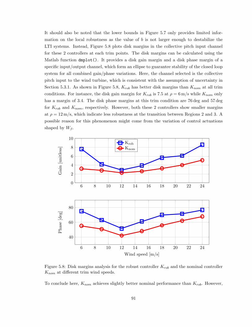
It should also be noted that the lower bounds in Figure 5.7 only provides limited infor-
mation on the local robustness as the value of b is not larger enough to destabilize the
LTI systems. Instead, Figure 5.8 plots disk margins in the collective pitch input channel
for these 2 controllers at each trim points. The disk margins can be calculated using the
Matlab function dmplot(). It provides a disk gain margin and a disk phase margin of a
specific input/output channel, which form an ellipse to guarantee stability of the closed loop
system for all combined gain/phase variations. Here, the channel selected is the collective
pitch input to the wind turbine, which is consistent with the assumption of uncertainty in
Section 5.3.1. As shown in Figure 5.8, Krob has better disk margins than Knom at all trim
conditions. For instance, the disk gain margin for Krob is 7.5 at ρ = 6 m/s while Knom only
has a margin of 3.4. The disk phase margins at this trim condition are 76 deg and 57 deg
for Krob and Knom, respectively. However, both these 2 controllers show smaller margins
at ρ = 12 m/s, which indicate less robustness at the transition between Regions 2 and 3. A
possible reason for this phenomenon might come from the variation of control actuations
shaped by Wβ.
6 8 10 12 14 16 18 20 22 240
2
4
6
8
10
Gai
n[u
nit
less
]
Krob
Knom
6 8 10 12 14 16 18 20 22 24
40
60
80
Wind speed [m/s]
Ph
ase
[deg
]
Figure 5.8: Disk margins analysis for the robust controller Krob and the nominal controllerKnom at different trim wind speeds.
To conclude here, Knom achieves slightly better nominal performance than Krob. However,
91

Krob has much better robust performance when the effect of uncertainty can not be ignored
in the model. The difference between these 2 controllers will be verified by simulations in
the following section.
5.4 Simulations and Analysis
5.4.1 Simulations for APC
Both the robust controller Krob and the nominal controller Knom will be tested in the FAST
simulation environment. As these two designs were based on a simplified model of the C96
turbine, structural modes in the FAST simulation include the rotor position, drive train
torsion and first tower fore-aft mode. Therefore, the model used for simulations contains 3
DOFs. The objective of simulation is to verify the APC performance without uncertainty
in the turbine model. Similar to the set up in Section 3.5, a turbulence level of 5 % is used
to generate all wind profiles in TurbSim. In addition, simulation results in the first 60 s will
be ignored due to the effect of initial response.
For simplicity, simulation results in 2 different wind speeds are shown in Figures 5.9 and
5.10, which cover Regions 2 and 3 wind conditions. In the first simulation, the mean wind
speed is 9m/s. Krob and Knom are simulated to track a power reference as shown by the
solid green curve in the second subplot of Figure 5.9. This command steps from 700 kW
to 1300 kW at t = 210 s, then drops to 100 kW at t = 360 s and finally steps back to
700 kW at t = 560 s. It is seen that Krob and Knom have similar responses to the reference
signal. The 90 % settling time to the step command is around 20 s, which is reasonable
for the objective of APC. It should be noted that the maximum available power at 9m/s
is 1426 kW, according to Equation 2.1. Therefore, the wind turbine might not be able to
track the power reference of 1300 kW accurately from t = 210 s to 360 s, if the wind speed
drops too much due to the turbulence. To prevent possible instability of the system in this
situation, the power reference signal is saturated by the maximum available power, which
can be calculated based on measurements of the trim wind speed. It is seen that the power
output drops at t = 300 s when the wind speed is close to 8 m/s and the system maintains
stable due to the saturation. The generator speed is also affected by the wind turbulence.
As shown in the third subplot of Figure 5.9, both Krob and Knom try to track the rated
generator speed when the wind speed is above 9 m/s. In contrast, the generator speed tracks
a time varying command that is proportional to the wind speed when it goes below 9 m/s.
The second simulation is performed at an average wind speed of 18m/s which is above
the rated value. In traditional operations as discussed in Chapter 3, the C96 wind turbine
tries to track the rated generator speed and maintain the power output of 2500 kW at this
wind speed. Therefore, in the mode of APC, Krob and Knom should be able to track a
92

100 150 200 250 300 350 400 450 500 550 600 650
8
9
10v
[m/s]
100 150 200 250 300 350 400 450 500 550 600 6500
500
1,000
1,500
P[k
W]
Knom
Krob
Reference
100 150 200 250 300 350 400 450 500 550 600 650
1,060
1,080
1,100
1,120
1,140
ωg
[RP
M]
100 150 200 250 300 350 400 450 500 550 600 6500
5
10
15
τg
[kN
m]
100 150 200 250 300 350 400 450 500 550 600 6500
5
10
15
Time [s]
β[d
eg]
Figure 5.9: Simulations for APC using the robust controller Krob and the nominal controllerKnom at ρ = 9 m/s.
93

power reference command varying from 0 to the rated value. Here, the power reference is
set as shown by the solid green curve in the second subplot of Figure 5.10. It steps from
1500 kW to 2300 kW at t = 210 s, then drops to 700 kW at t = 360 s and finally steps back
to 1500 kW at t = 560 s. Results of the power reference tracking for Krob and Knom are
also shown in this subplot of Figure 5.10. Comparing to the nominal controller Knom, Krob
shows a slower response to the reference. This difference can be explained by the sensitivity
function of power reference tracking, as shown in the right subplot of Figure 5.6. Specifically,
Krob has a smaller bandwidth for tracking the reference signal at this trim condition. A
further comparison on the fourth subplot of Figure 5.10 shows that the limited bandwidth
of actuation on the generator torque leads to the slow response of Krob. As the wind speed is
kept above rated in the simulation, the generator speed command is held fixed at the rated
value. Both Krob and Knom show good tracking performance of this constant command,
as shown in the third subplot of Figure 5.10. The actuations on the blade pitch are also
similar between these 2 controllers.
5.4.2 Worst Case Performance Simulations
Simulations in Section 5.4.1 show that the robust controller Krob has similar performance
as the nominal controller Knom for the objective of APC. These results were based on the
assumption that there is no uncertainty in the turbine model. Therefore, it is meaningful
to explore robust performance of Krob and Knom. The basic idea here is to find out a worst
case uncertainty model ∆wc with a fixed norm bound for each controller and then compare
the performance degradation after ∆wc is considered in simulations. However, the robust
performance condition in Section 4.4.1 does not provide any information on the worst case
uncertainty model for LPV systems. As a compromise, the Robust Control toolbox [108] is
used again to find out ∆wc for the LTI system at a specific trim point. Here, the trim point
is chosen at ρ = 15 m/s to get the closed loop LTI model. As described in Section 5.3.1,
the uncertainty in the blade pitch input channel is assumed to be LTI and normalized
as ‖∆‖ ≤ 1. It can be modeled using the command ultidyn() and interconnected with
the nominal system. This interconnected uncertain system is analyzed using the function
wcgain() which provides detailed information on the worst case gain and the corresponding
model of ∆wc. However, it should be noted that the worst case uncertainty ∆wc might be
different for Krob and Knom.
These 2 controllers are first simulated in FAST without ∆wc interconnected to the system
and the average wind speed is 15m/s with 5 % of turbulence. In the next step, ∆wc is
included in the system with Krob and Knom for simulations. The performance degradation
is analyzed based on the error of output yu = y0 − ywc. Here y0 and ywc are outputs of
simulation without and without ∆wc. Figure 5.11 shows the error of power output Pu for
94

100 150 200 250 300 350 400 450 500 550 600 650
16
18
20
22v
[m/s]
100 150 200 250 300 350 400 450 500 550 600 650500
1,000
1,500
2,000
2,500
P[k
W]
Knom
Krob
Reference
100 150 200 250 300 350 400 450 500 550 600 650
1,120
1,140
ωg
[RP
M]
100 150 200 250 300 350 400 450 500 550 600 650
10
15
20
τg
[kN
m]
100 150 200 250 300 350 400 450 500 550 600 65014
16
18
20
22
24
Time [s]
β[d
eg]
Figure 5.10: Simulation for APC using the robust controller Krob and the nominal controllerKnom at ρ = 18 m/s.
95

Krob and Knom. It is clear that ∆wc leads to large variation of Pu for Knom. Analysis results
for other outputs signals show the similar conclusion and are therefore not plotted here.
100 150 200 250 300 350 400 450 500 550 600 650
−20
−10
0
10
20
Time [s]
Pu
[kW
]Knom
Krob
Figure 5.11: Error on the power output with ∆wc using the robust controller Krob and thenominal controller Knom.
To further evaluate these errors, define the root mean square (RMS) of the error yu as:
yRMS =
(1
T
∫ T
0|yu|2dt
) 12
(5.4)
where T is the simulation time. This metric is applied to the generator speed, power output
and blade pitch angle. The results are shown in Table 5.2, which provides a quantitative
comparison between Krob and Knom. It is seen that Krob has significantly prevented the
performance degradation due to the worst case uncertainty. In addition, the damage equiv-
alent load (DEL) is also calculated for the low speed shaft torque. The values in the last
row of Table 5.2 show increments of DEL after the ∆wc was included in the model. It is
noted that the DEL for Knom has increased by 74.12 %, while this value for Krob is only
34.39 %. Apparently, Krob shows better robust performance than Knom on load reduction.
Table 5.2: Performance degradation with ∆wc.Description Knom Krob
RMS Power Error [kW] 6.2196 4.0241RMS Speed Error [RPM] 3.8464 1.9653RMS Pitch Angle [deg] 0.8642 0.4466Low Speed Shaft DEL Increase 74.12 % 34.39 %
96

Chapter 6
Conclusions
This thesis proposes a uniform MIMO control framework for wind turbines using the robust
linear parameter varying (LPV) design method. This framework takes multiple objectives in
different wind conditions into a systematic consideration, such that existing results based
on SISO linear control design can be integrated together with stability and performance
guarantee. As a first step, Chapter 3 proposes an LPV controller that is able to maximize
the power generation in Region 2 and track the rated generator speed in Region 3. Con-
siderations on load reduction are also included in the MIMO control structure. The use of
recently developed LPV toolbox in Matlab [18] ensures that the designed controller meets
objectives in different wind conditions and provides better load reduction performance than
the baseline controller.
A further step for the proposed LPV design is to ensure enough robustness of the system.
However, robust synthesis algorithms like µ-synthesis [20] is not directly available for LPV
systems and existing theories for robust LPV control are still incomplete. Therefore, Chap-
ter 4 proposes a robust synthesis algorithm for a class of uncertain LPV system, using the
theory of integral quadratic constraints (IQCs). The robust synthesis problem leads to a
non-convex optimization and the proposed algorithm is a coordinate-wise descent similar
to the well-known DK iteration for µ synthesis. Specifically, the proposed algorithm alter-
nates between an LPV synthesis step and an IQC analysis step. Both steps can be efficiently
solved as semidefinite programs. It is shown that the proposed algorithm ensures that the
robust performance is non-increasing at each iteration step.
This robust synthesis algorithm is used in Chapter 5 to design an LPV controller to pro-
vide APC. The control architecture is proposed by slightly modifying the LPV controller
for traditional operations in Chapter 3, with only one extra feedback loop for power ref-
erence tracking. The design procedure is therefore significantly simplified as some of the
97

tuning results in Chapter 3 can be directly inherited for APC. In addition, a multiplica-
tive uncertainty is considered in the blade pitch input channel of the turbine model. The
synthesized robust LPV controller shows similar performance on APC as a nominal LPV
controller designed without considerations of uncertainty. However, the robust controller
has much better performance when the worst case uncertainty is added to the system dy-
namics. Therefore, the robust LPV controller has guaranteed performance on APC, even
with perturbed system dynamics.
Overall, the robust LPV design framework proposed in this thesis provides a uniform control
architecture for wind turbines. This architecture, along with the unified design flow from
modeling, weights tuning to simulation, makes possible improvements in the future a natural
extension of the existing design. For example, it is possible to construct extra feedback loops
in this architecture for further load reduction, as sensors for turbine loads monitoring are
incorporated in the system. The popular individual pitch control can also be included to
decrease the periodic load on turbine blades. At the same time, more uncertainties can be
considered in the design to ensure robust performance of the controller, such as parametric
uncertainty in the turbine model, saturation/rate-limitation for actuators, etc.
Another important direction for future works is to improve efficiency of the robust synthesis
algorithm in Chapter 4. As shown in Chapter 5, this algorithm takes much longer time for
computation than the nominal synthesis algorithm included in the LPV toolbox. Therefore,
there were only 2 DOFs considered in the turbine model to simplify the APC design.
This is a critical bottleneck for applications of the robust synthesis algorithm, as the time
consumption will be unacceptable for more complicated designs. As the robust performance
bound γ enters into the matrix inequality bilinearly, it leads to a quasi-convex optimization
problem. It is therefore possible to solved the analysis step more efficiently using existing
method than the current bisection search.
98

Bibliography
[1] “World Wind Energy Report 2012,” Proceedings of the 12 th World Energy Confer-
ence, World Wind Energy Associtation, Havana, Cuba, 2013.
[2] “Eolos wind energy research consortium,” http://www.eolos.umn.edu/.
[3] “Wind turbine components,” http://www.alternative-energy-
news.info/images/technical/wind-turbine.jpg.
[4] Aho, J., Buckspan, A., Laks, J., Fleming, P., Jeong, Y., Dunne, F., Churchfield,
M., Pao, L., and Johnson, K., “A Tutorial of Wind Turbine Control for Supporting
Grid Frequency through Active Power Control,” Proceedings of American Control
Conference, IEEE, 2012, pp. 3120–3131.
[5] Lindenberg, S., Smith, B., and O’Dell, K., “20% wind energy by 2030,” National
Renewable Energy Laboratory (NREL), US Department of Energy, Renewable Energy
consulting Services, Energetics Incorporated , 2008.
[6] Crabtree, G., Misewich, J., Ambrosio, R., Clay, K., DeMartini, P., James, R., Lauby,
M., Mohta, V., Moura, J., Sauer, P., et al., “Integrating Renewable Electricity on the
Grid,” AIP Conference Proceedings-American Institute of Physics, Vol. 1401, 2011,
p. 387.
[7] Mai, T., Wiser, R., Sandor, D., Brinkman, G., Heath, G., Denholm, P., Hostick, D.,
Darghouth, N., Schlosser, A., and Strzepek, K., “Exploration of High-Penetration Re-
newable Electricity Futures. Vol. 1 of Renewable Electricity Futures Study,” National
Renewable Energy Laboratory, Golden, CO, Tech. Rep. NREL/TP-6A20-52409-1 ,
2012.
[8] Burton, T., Sharpe, D., Jenkins, N., and Bossanyi, E., Wind Energy Handbook , John
Wiley & Sons, 1st ed., 2001.
[9] Bossanyi, E. A., “Individual Blade Pitch Control for Load Reduction,” Wind Energy ,
Vol. 6, No. 2, 2003, pp. 119–128.
99

[10] Bossanyi, E., “Wind turbine control for load reduction,” Wind energy , Vol. 6, No. 3,
2003, pp. 229–244.
[11] Darrow, J., Johnson, K., and Wright, A., “Design of a tower and drive train damping
controller for the three-bladed controls advanced research turbine operating in design-
driving load cases,” Wind Energy , Vol. 14, No. 4, 2011, pp. 571–601.
[12] Dıaz de Corcuera, A., Pujana-Arrese, A., Ezquerra, J., Milo, A., and Landaluze, J.,
“Linear models-based LPV modelling and control for wind turbines,” Wind Energy ,
Vol. 18, No. 7, 2015, pp. 1151–1168.
[13] Licari, J., Ugalde-Loo, C. E., Ekanayake, J. B., and Jenkins, N., “Comparison of the
performance and stability of two torsional vibration dampers for variable-speed wind
turbines,” Wind Energy , Vol. 18, No. 9, 2015, pp. 1545–1559.
[14] Boyd, S., El Ghaoui, L., Feron, E., and Balakrishnan, V., Linear Matrix Inequalities
in System and Control Theory , Siam, 1994.
[15] Gahinet, P. and Apkarian, P., “A linear matrix inequality approach to H∞ control,”
International journal of robust and nonlinear control , Vol. 4, No. 4, 1994, pp. 421–448.
[16] Ossmann, D., Theis, J., and Seiler, P., “Robust Control Design For Load Reduction
on a Liberty Wind Turbine,” submitted to the ASME Dynamic Systems and Control
Conference, 2016.
[17] Jonkman, J. and Buhl, M., FAST User’s Guide, National Renewable Energy Labo-
ratory, Golden, Colorado, 2005.
[18] Hjartarson, A., Seiler, P., and Packard, A., “LPVTools: A toolbox for modeling,
analysis, and synthesis of parameter varying control systems,” IFAC-PapersOnLine,
Vol. 48, No. 26, 2015, pp. 139–145.
[19] Megretski, A. and Rantzer, A., “System Analysis via Integral Quadratic Constraints,”
IEEE Trans. on Automatic Control , Vol. 42, 1997, pp. 819–830.
[20] Zhou, K., Doyle, J., and Glover, K., Robust and Optimal Control , Prentice-Hall, 1996.
[21] Hardy, C., “Renewable energy and role of Marykirks James Blyth,” The courier. DC
Thomson & Co. Ltd, Dundee (06/07/2013), 2010.
[22] “Mr. Brush’s Windmill Dynamo,” Scientific American, Dec. 1890.
[23] Østergaard, K. Z., Robust, Gain-Scheduled Control of Wind Turbines, Ph.D. the-
sis, Automation and Control, Department of Electronic Systems, Aalborg University,
2008.
100

[24] Ozdemir, A. A., Preview Control for Wind Turbines, Ph.D. thesis, University of
Minnesota, 2013.
[25] “The world’s 10 biggest wind turbines,” Jan. 2014, http://www.power-
technology.com/features/featurethe-worlds-biggest-wind-turbines-4154395/.
[26] Manwell, J., McGowan, J., and Rogers, A., Wind Energy Explained: Theory, Design,
and Application, Wiley, 2010.
[27] Bossanyi, E., “The design of closed loop controllers for wind turbines,” Wind Energy ,
Vol. 3, 2000, pp. 149–163.
[28] Laks, J., Pao, L., and Wright, A., “Control of Wind Turbines: Past, Present, and
Future,” Proceedings of American Control Conference, 2009, pp. 2096–2103.
[29] Johnson, K., Pao, L., Balas, M., and Fingersh, L., “Control of variable-speed wind
turbines: standard and adaptive techniques for maximizing energy capture,” IEEE
Control System Magazine, Vol. 26, No. 3, 2006, pp. 70–81.
[30] Buhl Jr, M. L. and Manjock, A., “A comparison of wind turbine aeroelastic codes used
for certification,” Conference Paper National Renewable Energy Laboratory, Golden,
CO, Report No. NREL/CP-500-39113 , 2006.
[31] Clough, R. W. and Penzien, J., “Dynamics of structures,” Tech. rep., 1975.
[32] Meirovitch, L., Dynamics and control of structures, John Wiley & Sons, 1990.
[33] Jonkman, B. J., “TurbSim user’s guide: Version 1.50,” 2009.
[34] Commission, I. E. et al., “IEC 61400-1: Wind turbines part 1: Design requirements,”
International Electrotechnical Commission, 2005.
[35] Moriarty, P. J. and Hansen, A. C., AeroDyn theory manual , Citeseer, 2005.
[36] Sørensen, J. N., “Blade-Element/Momentum Theory,” General Momentum Theory
for Horizontal Axis Wind Turbines, Springer, 2016, pp. 99–121.
[37] Johnson, W., “Helicopter TheoryPrinceton University Press,” Princeton, New Jersey,
USA, 1980.
[38] Stol, K., Balas, M., and Bir, G., “Floquet modal analysis of a teetered-rotor wind
turbine,” Journal of solar energy engineering , Vol. 124, No. 4, 2002, pp. 364–371.
[39] Bir, G., “Multiblade coordinate transformation and its application to wind turbine
analysis,” ASME Wind Energy Symposium, 2008.
101

[40] Stol, K. A., Moll, H.-G., Bir, G., and Namik, H., “A comparison of multi-blade
coordinate transformation and direct periodic techniques for wind turbine control
design,” Proceedings of the 47th AIAA/ASME , 2009.
[41] Bir, G. S., “User’s guide to MBC3: Multi-blade coordinate transformation code for
3-bladed wind turbine,” 2010.
[42] Selvam, K., Kanev, S., van Wingerden, J., van Engelen, T., and Verhaegen, M.,
“Feedback–feedforward individual pitch control for wind turbine load reduction,” In-
ternational Journal of Robust and Nonlinear Control , Vol. 19, No. 1, 2009, pp. 72–91.
[43] Pao, L. Y. and Johnson, K. E., “A tutorial on the dynamics and control of wind
turbines and wind farms,” American Control Conference, IEEE, 2009, pp. 2076–2089.
[44] Harris, M., Hand, M., and Wright, A., “Lidar for turbine control,” National Renewable
Energy Laboratory, Golden, CO, Report No. NREL/TP-500-39154 , 2006.
[45] Simley, E., Pao, L. Y., Frehlich, R., Jonkman, B., and Kelley, N., “Analysis of wind
speed measurements using continuous wave LIDAR for wind turbine control,” Pro-
ceedings of the 49th AIAA Aerospace Sciences Meeting , 2011.
[46] Wang, N., Johnson, K. E., and Wright, A. D., “FX-RLS-based feedforward control
for LIDAR-enabled wind turbine load mitigation,” Control Systems Technology, IEEE
Transactions on, Vol. 20, No. 5, 2012, pp. 1212–1222.
[47] Ozdemir, A. A., Seiler, P., and Balas, G. J., “Design tradeoffs of wind turbine preview
control,” Control Systems Technology, IEEE Transactions on, Vol. 21, No. 4, 2013,
pp. 1143–1154.
[48] Schlipf, D., Schlipf, D. J., and Kuhn, M., “Nonlinear model predictive control of wind
turbines using LIDAR,” Wind Energy , Vol. 16, No. 7, 2013, pp. 1107–1129.
[49] Rezaei, V., “LIDAR-based robust wind-scheduled control of wind turbines,” American
Control Conference, IEEE, 2014, pp. 4416–4421.
[50] Bossanyi, E., Kumar, A., and Hugues-Salas, O., “Wind turbine control applications
of turbine-mounted LIDAR,” Journal of Physics: Conference Series, Vol. 555, IOP
Publishing, 2014, p. 012011.
[51] Lim, D.-W., Mantell, S. C., and Seiler, P. J., “Wireless structural health monitoring
of wind turbine blades using an energy harvester as a sensor,” Proceedings of the 32nd
ASME wind energy symposium. MD: National Harbor , 2014.
102
[52] Ozdemir, A. A., Seiler, P. J., and Balas, G. J., “Performance of Disturbance Aug-
mented Control Design in Turbulent Wind Conditions,” Mechatronics, Vol. 21, No. 4,
2011, pp. 634 – 644.
[53] Fleming, P. A., Van Wingerden, J.-W., and Wright, A. D., Comparing state-space
multivariable controls to multi-siso controls for load reduction of drivetrain-coupled
modes on wind turbines through field-testing , American Institute of Aeronautics and
Astronautics (AIAA), 2012.
[54] Bianchi, F. D., De Battista, H., and Mantz, R. J., “Robust Multivariable Gain-
Scheduled Control of Wind Turbines for Variable Power Production.” International
Journal of Systems Control , Vol. 1, No. 3, 2010.
[55] Inthamoussou, F. A., Bianchi, F. D., De Battista, H., and Mantz, R. J., “LPV wind
turbine control with anti-windup features covering the complete wind speed range,”
Energy Conversion, IEEE Transactions on, Vol. 29, No. 1, 2014, pp. 259–266.
[56] Apkarian, P. and Gahinet, P., “A Convex Characterization of Gain-Scheduled H∞
Controllers,” IEEE Trans. on Automatic Control , Vol. 40, 1995, pp. 853–864.
[57] Wu, F., Control of Linear Parameter Varying Systems, Ph.D. thesis, University of
California, Berkeley, 1995.
[58] Wu, F., Yang, X. H., Packard, A., and Becker, G., “Induced L2 norm control for LPV
systems with bounded parameter variation rates,” International Journal of Robust
and Nonlinear Control , Vol. 6, 1996, pp. 983–998.
[59] Hoffmann, C. and Werner, H., “A survey of linear parameter-varying control ap-
plications validated by experiments or high-fidelity simulations,” Control Systems
Technology, IEEE Transactions on, Vol. 23, No. 2, 2015, pp. 416–433.
[60] Bianchi, F., Mantz, R., and Christiansen, C., “Control of variable-speed wind turbines
by LPV gain scheduling,” Wind Energy , Vol. 7, No. 1, 2004, pp. 1–8.
[61] Østergaard, K. Z., Stoustrup, J., and Brath, P., “Linear parameter varying control
of wind turbines covering both partial load and full load conditions,” International
Journal of Robust and Nonlinear Control , Vol. 19, No. 1, 2009, pp. 92–116.
[62] Bianchi, F. D., De Battista, H., and Mantz, R. J., “Robust Multivariable Gain-
Scheduled Control of Wind Turbines for Variable Power Production.” International
Journal of Systems Control , Vol. 1, No. 3, 2010.
103

[63] Bobanac, V., Jelavic, M., and Peric, N., “Linear Parameter Varying Approach to
Wind Turbine Control,” 14th International Power Electronics and Motion Control
Conference, 2010, pp. T12–60–T12–67.
[64] Bakka, T., Karimi, H.-R., and Christiansen, S., “Linear parameter-varying modelling
and control of an offshore wind turbine with constrained information,” Control Theory
& Applications, IET , Vol. 8, No. 1, 2014, pp. 22–29.
[65] Sloth, C., Esbensen, T., and Stoustrup, J., “Robust and fault-tolerant linear
parameter-varying control of wind turbines,” Mechatronics, Vol. 21, No. 4, 2011,
pp. 645–659.
[66] Adegas, F. D., Sonderby, I. B., Hansen, M. H., and Stoustrup, J., “Reduced-order
LPV model of flexible wind turbines from high fidelity aeroelastic codes,” Control
Applications (CCA), 2013 IEEE International Conference on, IEEE, 2013, pp. 424–
429.
[67] Shirazi, F. A., Grigoriadis, K. M., and Viassolo, D., “An integrated approach towards
structural and LPV controller design in wind turbines,” American Control Conference
(ACC), 2012 , IEEE, 2012, pp. 5789–5794.
[68] Apkarian, P. and Adams, R., “Advanced gain-scheduling techniques for uncertain
systems,” IEEE Trans. on Control Systems Technology , Vol. 6, No. 1, 1998, pp. 21–
32.
[69] Packard, A., “Gain scheduling via linear fractional transformations,” Systems & Con-
trol Letters, Vol. 22, No. 2, 1994, pp. 79–92.
[70] Safonov, M. G., Limebeer, D. J. N., and Chiang, R. Y., “Simplifying the H∞ theory
via loop-shifting, matrix-pencil and descriptor concepts,” International Journal of
Control , Vol. 50-6, 1989, pp. 2467–2488.
[71] Mikkelsen, T., Hansen, K., Angelou, N., Sjoholm, M., Harris, M., Hadley, P., Scullion,
R., Ellis, G., and Vives, G., “Lidar wind speed measurements from a rotating spinner,”
Proc. European Wind Energy Conference, Warsaw, Poland , 2010.
[72] Knudsen, T., Bak, T., and Soltani, M., “Prediction models for wind speed at turbine
locations in a wind farm,” Wind Energy , Vol. 14, No. 7, 2011, pp. 877–894.
[73] M. Buhl, J., “MCrunch User’s Guide for Version 1.00,” May 2008,
http://www.nrel.gov/docs/fy08osti/43139.pdf.
104

[74] Moreno, C., Seiler, P., and Balas, G., “Linear Parameter Varying Model Reduction for
Aeroservoelastic Systems,” AIAA Atmospheric Flight Mechanics Conference, 2012,
pp. Paper No. AIAA–2012–4859.
[75] Wang, S. and Seiler, P., “Gain Scheduled Active Power Control for Wind Turbines,”
AIAA Atmospheric Flight Mechanics Conference, 2014, pp. Paper No. AIAA–2014–
1220.
[76] Balas, G., Chiang, R., Packard, A., and Safonov, M., “Robust Control Toolbox 3
User’s Guide,” Tech. rep., The Math Works, Inc., 2007.
[77] Pfifer, H. and Seiler, P., “Robustness Analysis of Linear Parameter Varying Systems
Using Integral Quadratic Constraints,” accepted to the International Journal of Robust
and Nonlinear Control , 2014.
[78] Pfifer, H. and Seiler, P., “Robustness Analysis of Linear Parameter Varying Systems
Using Integral Quadratic Constraints,” American Control Conference, 2014, pp. 4476–
4481.
[79] Cantoni, M., Jonsson, U., and Khong, S., “Robust stability analysis for feedback
interconnections of time-varying linear systems,” SIAM J. of Control Optim., Vol. 51,
No. 1, 2013, pp. 353–379.
[80] Veenman, J. and Scherer, C., “On robust LPV controller synthesis: A dynamic inte-
gral quadratic constraint based approach,” IEEE Conference on Decision and Con-
trol , 2010, pp. 591–596.
[81] Veenman, J. and Scherer, C., “IQC-synthesis with general dynamic multipliers,” In-
ternational Journal of Robust and Nonlinear Control , Vol. 24, 2012, pp. 3027–3056.
[82] Scherer, C. and Kose, I., “Gain-scheduled control synthesis using dynamic D-scales,”
IEEE Trans. on Automatic Control , Vol. 57, 2012, pp. 2219–2234.
[83] Scherer, C., “Gain-scheduled synthesis with dynamic positive real multipliers,” IEEE
Conference on Decision and Control , 2012, pp. 6641–6646.
[84] Wang, S., Pfifer, H., and Seiler, P., “Robust Synthesis for Linear Parameter Varying
Systems Using Integral Quadratic Constraints,” IEEE Conference on Decision and
Control , 2014, pp. 4789–4794.
[85] Yakubovich, V., “S-procedure in nonlinear control theory,” Vestnik Leningrad Univ.,
1971, pp. 62–77.
105

[86] Scherer, C. and Wieland, S., “Linear Matrix Inequalities in Control,” Lecture notes for
a course of the dutch institute of systems and control, Delft University of Technology,
2004.
[87] Fu, M., Dasgupta, S., and Soh, Y., “Integral quadratic constraint approach vs. mul-
tiplier approach,” Automatica, Vol. 41, 2005, pp. 281–287.
[88] Carrasco, J., Heath, W., and Lanzon, A., “Factorization of multipliers in passivity
and IQC analysis,” Automatica, Vol. 48, No. 5, 2012, pp. 909–916.
[89] Megretski, A., “KYP Lemma for Non-Strict Inequalities and the associated Minimax
Theorem,” Arxiv, 2010.
[90] Scherer, C. and Kose, I., “Robustness with dynamic IQCs: An exact state-space char-
acterization of nominal stability with applications to robust estimation,” Automatica,
Vol. 44, 2008, pp. 1666–1675.
[91] Turner, M. and Kerr, M., “L2 gain bounds for systems with sector bounded and slope-
restricted nonlinearities,” International Journal of Robust and Nonlinear Control ,
Vol. 22, No. 13, 2012, pp. 1505–1521.
[92] Young, P., Robustness with Parametric and Dynamic Uncertainty , Ph.D. thesis, Cal-
ifornia Institute of Technology, 1993.
[93] Young, P., “Controller Design with Mixed Uncertainties,” American Control Confer-
ence, 1994, pp. 2333–2337.
[94] Schaft, A. and A.J.Schaft, L2-gain and passivity in nonlinear control , Springer-Verlag
New York, Inc., 1999.
[95] Jonsson, U., Robustness analysis of uncertain and nonlinear systems, Ph.D. thesis,
Lund Institute of Technology, 1996.
[96] Skogestad, S. and Postlethwaite, I., Multivariable Feedback Control , John Wiley and
Sons, Chichester, 2005.
[97] Rebours, Y., Kirschen, D., Trotignon, M., and Rossignol, S., “A Survey of Freqency
and Voltage Control Ancillary Services-Part I: Technical Features,” IEEE Transac-
tions on Power Systems, Vol. 22, No. 1, 2007, pp. 350–357.
[98] Greedy, L., “Review of electrical drive-train topologies,” Project UpWind, Mekelweg,
the Netherlands and Aalborg East, Denmark, Tech. Rep, 2007.
[99] Nelson, R. J., “Frequency-Responsive Wind Turbine Output Control,” 2011, U.S.
Patent 0 001 318.
106

[100] Keung, P.-K., Li, P., Banakar, H., and Ooi, B. T., “Kinetic Energy of Wind Turbine
Generators for System Frequency Support,” IEEE Transactions on Power Systems,
Vol. 24, No. 1, 2009, pp. 279–287.
[101] Juankorena, X., Esandi, I., Lopez, J., and Marroyo, L., “Method to Enable Vari-
able Speed Wind Turbine Primary Regulation,” International Conference on Power
Engineering, Energy and Electrical Drives, 2009 , IEEE, 2009, pp. 495–500.
[102] Aho, J., Buckspan, A., Pao, L., and Fleming, P., “An Active Power Control System for
Wind Turbines Capable of Primary and Secondary Frequency Control for Supporting
Grid Reliability,” 51st AIAA Aerospace Sciences Meeting including the New Horizons
Forum and Aerospace Exposition, 2013, pp. AIAA 2013–0456.
[103] Acedo Sanchez, J., Carcar, M., Lusarreta, M., Perez Barbachano, J., Simon Segura,
S., Sole Lopez, D., Zabaleta Maeztu, M., Marroyo Palomo, L., Lopez Taberna, J.,
et al., “Method of Operation of A Wind Turbine to Guarantee Primary or Secondary
Regulation in An Electric Grid,” 2011, U.S. Patent 0 057 445.
[104] Jeong, Y., Johnson, K., and Fleming, P., “Comparison and testing of power reserve
control strategies for grid-connected wind turbines,” Wind Energy , 2013.
[105] Tarnowski, G., Kjær, P., Dalsgaard, S., and Nyborg, A., “Regulation and Frequency
Response Service Capability of Modern Wind Power Plants,” Proceedings of IEEE
Power and Energy Society General Meeting , 2010, pp. 1–8.
[106] Wang, S. and Seiler, P., “LPV Active Power Control and Robust Analysis for Wind
Turbines,” 33rd Wind Energy Symposium, 2015, p. 1210.
[107] Pfifer, H. and Seiler, P., “Robustness Analysis of Linear Parameter Varying Systems
Using Integral Quadratic Constraints,” International Journal of Robust and Nonlinear
Control , Vol. 25, 2015, pp. 2843–2864.
[108] Balas, G., Chiang, R., Packard, A., and Safonov, M., “MATLAB robust control
toolbox 3, users guide,” 2010.
[109] Peni, T. and Seiler, P., “Computation of lower bounds for the induced L2 norm of
LPV systems,” Vol. 26, No. 4, 2016, pp. 646–661.
[110] Francis, B., A Course in H∞ Control Theory , Springer-Verlag, 1987.
[111] Seiler, P., “Stability Analysis with Dissipation Inequalities and Integral Quadratic
Constraints,” accepted to the IEEE Trans. on Automatic Control , 2013.
[112] Bart, H., Gohberg, I., and Kaashoek, M., Minimal Factorization of Matrix and Op-
erator Functions, Birkhauser, 1979.
107

[113] Meinsma, G., “J-spectral Factorization and Equalizing Vectors,” Systems and Control
Letters, Vol. 25, 1995, pp. 243–249.
[114] Engwerda, J., LQ Dynamic Optimization and Differential Games, Wiley, 1st ed.,
2005.
[115] Engwerda, J., “Uniqueness conditions for the affine open-loop linear quadratic differ-
ential game,” Automatica, Vol. 44, 2008, pp. 504–511.
[116] Willems, J., “Least squares stationary optimal control and the algebraic Riccati e-
quation,” IEEE Trans. on Aut. Control , Vol. 16, 1971, pp. 621–634.
108

Appendix A
IQC Factorizations
Two factorizations of the frequency domain IQC multiplier Π are provided in Lemma 4
and Lemma 5. The first factorization given by Lemma 4 only assumes Π to be rational
and uniformly bounded. However, this factorization (Ψ,M) does not, in general, yield a
valid time domain IQC. The second factorization given by Lemma 5 is called a J-spectral
factorization and it requires additional assumptions on Π. Lemma 6 shows that this J-
spectral factorization yields a valid time domain IQC.
Lemma 4. If Π = Π∼ ∈ RLm×m∞ then there exists real matrices A, B, Q, S, R of compatible
dimensions with A Hurwitz, Q = QT , and R = RT such that
Π(s) = [ BT (−sI−AT )−1 I ][Q S
ST R
] [(sI−A)−1B
I
](A.1)
Proof. The proof follows from arguments in Section 7.3 of [110]. Let (Aπ, Bπ, Cπ, Dπ) be
a minimal state-space realization for Π. Separate Π into its stable and unstable parts
Π = GS +GU +Dπ. Let (A, B, C, 0) denote a state-space realization for the stable part GS
so that A is Hurwitz. The assumptions on Π imply that GU has a state-space realization of
the form (−AT ,−CT , BT , 0) (Section 7.3 of [110]). Thus Π = GS +GU +Dπ can be written
as in Equation A.1 with Q = 0, S = CT and R = Dπ.
Lemma 4 provides a factorization of Π in the form Ψ∼MΨ where Ψ(s) :=[
(sI−A)−1BI
]and M :=
[Q S
ST R
]. The main construction in the proof is to separate the stable and
unstable parts of Π. This can be easily implemented in Matlab using the stabsep command.
This provides a factorization Π = Ψ∼MΨ where Ψ ∈ RHnz×m∞ is stable but non-square.
Moreover, this factorization (Ψ,M) does not, in general, yield a valid time domain IQC as
109

described in Definition 2. Lemma 5 below states another special factorization with some
additional assumptions on Π.
Lemma 5. Let Π = Π∼ ∈ RL(nv+nw)×(nv+nw)∞ be partitioned as
[Π11 Π12Π∼12 Π22
]where Π11 ∈
RLnv×nv∞ and Π22 ∈ RLnw×nw∞ . If Π11(jω) > 0 and Π22(jω) < 0 ∀ω ∈ R ∪ {∞}, then
(i) There exists real matrices A, B, Q, S, R of compatible dimensions with A Hurwitz,
Q = QT , and R = RT such that Π can be expressed as in Equation A.1.
(ii) R is nonsingular and there exists a unique real solution X = XT to the the following
ARE
ATX +XA− (XB + S)R−1(XB + S)T + Q = 0 (A.2)
such that A− BR−1(XB + S
)Tis Hurwitz.
(iii) Π has a factorization (Ψ,M) with M :=[Inv 00 −Inw
]and Ψ,Ψ−1 ∈ RH(nv+nw)×(nv+nw)
∞ .
A state-space realization of Ψ is given by(A, B, C, D
)where D is a solution of R =
DTMD and C := MD−T(BTX + ST
).
Proof. Conclusion (i) holds for any Π = Π∼ and follows from Lemma 4. Conclusions (ii)
and (iii) follow from Lemma 4 in [111].
The factorization in Conclusion (iii) is called a J-spectral factorization of Π. For this fac-
torization, Ψ is square, stable, and stably invertible. Existence conditions for a J-spectral
factor of Π are provided by the canonical factorization theorem in [112]. Chapter 7 of [110]
summarizes these results. Existence conditions for a J-spectral factor can also be specified
using the notion of an equalizing vector as defined in [113]. Lemma 5 above provides an
alternative existence condition for a J-spectral factorization in terms of definiteness prop-
erties on Π. Lemma 6 below states that the J-spectral factorization is a hard factorization
of Π. Thus a frequency domain IQC multiplier can, under some additional assumptions on
Π, be factorized to yield a valid time domain IQC. Lemma 6 also provides an additional
technical result that will be used in Chapter 4.
Lemma 6. Let Π = Π∼ ∈ RL(nv+nw)×(nv+nw)∞ be partitioned as
[Π11 Π12Π∼12 Π22
]where Π11 ∈
RLnv×nv∞ and Π22 ∈ RLnw×nw∞ . Assume Π11(jω) > 0 and Π22(jω) < 0 ∀ω ∈ R ∪ {∞}. Let
(Ψ,M) be the J-spectral factorization given in Conclusion (iii) of Lemma 5. Then,
110

(i) (Ψ,M) is a hard factorization of Π: If ∆ is a bounded, causal operator that satisfies the
frequency domain IQC specified by Π (Definition 1) then ∆ satisfies the time domain
IQC specified by (Ψ,M) (Definition 2).
(ii) The cost of the max/min game defined in Equation A.3 based on (Ψ,M) satisfies
J(xψ0) = 0.
J(xψ0) := supw∈Lnw2 [0,∞)
infv∈Lnv2 [0,∞)
∫ ∞0
z(t)TMz(t) dt (A.3)
subject to:
xψ = Axψ + B [ vw ] , xψ(0) = xψ0
z = Cxψ + D [ vw ]
Proof. Conclusion (i) follows from Theorem 2.4 in [89] or Theorem 4 in [111]. Conclusion
(ii) follows from Lemma 5 and the proof of Theorem 4 in [111]. J is the lower-value of a
two-player differential game and the proof of Conclusion (ii) given in [111] essentially relies
on results for LQ differential games [114,115].
111

Appendix B
Extended System State Matrices
A state-space realization for the extended system of Hρ and Ψ1/γ is given in Equation 4.9.
The state matrices for the extended system can be expressed in terms of the state matrices
for Hρ (Equation 4.7) and Ψ1/γ (Equation 4.8) as:
A(ρ) :=
[A(ρ) 0
γ−1BvCv(ρ) A
](B.1)
Bw(ρ) :=
[Bw(ρ)
γ−1BvDvw(ρ) + Bw
], Bd(ρ) :=
[Bd(ρ)
γ−1BvDvd(ρ)
](B.2)
Czk(ρ) :=[γ−1DzkvCv(ρ), Czk
], Ce(ρ) :=
[Ce(ρ), 0
](B.3)
Dzkw(ρ) := γ−1DzkvDvw(ρ) + Dzkw, Dew(ρ) := Dew(ρ) (B.4)
Dzkd(ρ) := γ−1DzkvDvd(ρ), Ded(ρ) := Ded(ρ) (B.5)
Similarly, the state-space realization for the extended system of Hρ and Ψλ is given in
Equation 4.14. These state matrices can be expressed in terms of the state matrices for
Hρ (Equation 4.7) and Ψλ (Equation 4.13). Only the output and feedthrough matrices
associated with the output zλ are changed. These are given by:
Czλ(ρ) :=[γ−1DzλvCv(ρ), Czλ
](B.6)
Dzλw(ρ) := γ−1DzλvDvw(ρ) + Dzλw (B.7)
Dzλd(ρ) := γ−1DzλvDvd(ρ) (B.8)
112

Appendix C
Proof of Lemma 1
Proof. (⇒) Assume P = P T satisfies Equation 4.15. The output zk from Ψ1/γ is a linear
function of (xψ, v, w) as defined in Equation 4.8:
zk = [ Czk γ−1Dzkv Dzkw ]
[xψvw
](C.1)
These variables (xψ, v, w) can, in turn, be expressed in terms of the extended system state
and inputs (x,w, d) as:xψvw
=
[0, I] 0 0
[Cv(ρ), 0] Dvw(ρ) Dvd(ρ)
[0, 0] I 0
[ xHxψ
]w
d
:= L(ρ)
[ xHxψ
]w
d
(C.2)
Thus, using the extended system state matrices defined in Appendix B, the second term of
the matrix inequality in Equation 4.15 can be rewritten as:
N∑k=1
λk
CTzkDTzkwDTzkd
Mk [ Czk Dzkw Dzkd ] = L(ρ)T
[Qλ Sλ
STλ Rλ
]L(ρ) (C.3)
Qλ, Sλ, and Rλ are defined in Equation 4.12. Substitute for Qλ using the ARE in Equa-
tion A.2. Rearrange terms in the matrix inequality to show that P := P +[
0 00 X
]satisfies
Equation 4.16.
This direction of the proof is completed by showing that P ≥ 0. Define the quadratic
function V (x0) := xT0 P x0. In addition, define the following quadratic cost functional V ∗(x0)
113

based on the extended system of Hρ and the rescaled factorization (Ψλ,Mλ):
V ∗(x0) := supw∈Lnw2 [0,∞)
∫ ∞0
zλ(t)TMλzλ(t) dt (C.4)
subject to:
x = A(ρ)x+ Bw(ρ)w, x(0) = x0
zλ = Czλ(ρ)x+Dzλw(ρ)w
The disturbance input of the extended system is neglected (d = 0) in this linear quadratic
optimization. Note that the extended system is stable since Hρ is stable (by assumption),
Ψλ is stable (by construction), and Ψλ is connected in an open loop fashion to Hρ. First we
show that V (x0) ≥ V ∗(x0) for all x0 ∈ RnH+nψ . This follows along the lines of Theorems 2
and 3 in [116] and hence the proof is only sketched. Let x(t), zλ(t) be the resulting solutions
of the extended system of Hρ and Ψλ for a given input w ∈ Lnw2 [0,∞), admissible trajectory
ρ ∈ T , and initial condition x0 ∈ RnH+nψ assuming d = 0. Multiply the matrix inequality in
Equation 4.16 on the left/right by
[x(t)w(t)
0
]Tand
[x(t)w(t)
0
]to show V (x(t))+zλ(t)TMλzλ(t) ≤ 0.
Integrate this inequality from t = 0 to t = T to obtain
V (x(T )) +
∫ T
0zλ(t)TMλzλ(t) dt ≤ V (x0) (C.5)
limT→∞ x(T ) = 0 for any w ∈ Lnw2 [0,∞) because the extended system is stable. Maximizing
the left side of Equation C.5 over w ∈ Lnw2 [0,∞) for T =∞ thus yields V (x0) ≥ V ∗(x0).
Next, consider the max/min game defined for the rescaled J-spectral factorization (Ψλ,Mλ):
J(xψ0) := supw∈Lnw2 [0,∞)
infv∈Lnv2 [0,∞)
∫ ∞0
zλ(t)TMλzλ(t) dt (C.6)
subject to:
xψ = Axψ + B [ vw ] , xψ(0) = xψ0
z = Czλxψ + Dzλ [ vw ]
where Dzλ := [Dzλv, Dzλw]. This max/min game is connected to the quadratic optimization
defined in Equation C.4. Specifically, restricting v in the max/min game to be the output
of Hρ generated by w ∈ L2, d = 0, and xH(0) = xH0 yields the quadratic optimization in
Equation C.4. This specific choice of v yields a value that is no lower than the infimum
over all possible v ∈ L2. Hence the max/min game yields the bound J(xψ0) ≤ V ∗(x0). By
Lemma 6, the cost of this max/min game is J(xψ0) = 0. Putting these results together
114

yields the following inequality
0 = J(xψ0) ≤ V ∗(x0) ≤ V (x0) := xT0 P x0 (C.7)
This holds for any x0 and thus P ≥ 0.
(⇐) This direction of the proof essentially involves reversing the algebraic rearrangement
to go from the matrix inequality in Equation 4.16 to the form in Equation 4.15.
115