arX

iv:1

505.

0656

2v3

[cs.

SY

] 1

Jul 2

016

1

Robust linear static anti-windupwith probabilistic certificates

Simone Formentin,Member, IEEE,Fabrizio Dabbene,Senior Member, IEEE,Roberto Tempo,Fellow, IEEE,Luca Zaccarian,Fellow, IEEE,and Sergio M. Savaresi,Senior Member, IEEE

Abstract—In this paper, we address robust static anti-windupcompensator design and performance analysis for saturatedlinear closed loops in the presence of nonlinear probabilistic pa-rameter uncertainties via randomized techniques. The proposedstatic anti-windup analysis and robust performance synthesis cor-respond to several optimization goals, ranging from minimizationof the nonlinear input/output gain to maximization of the stabilityregion or maximization of the domain of attraction. We alsointroduce a novel paradigm accounting for uncertainties in theenergy of the disturbance inputs.

Due to the special structure of linear static anti-windup design,wherein the design variables are decoupled from the Lyapunovcertificates, we introduce a significant extension, calledscenariowith certificates (SwC), of the so-called scenario approach foruncertain optimization problems. This extension is of inde-pendent interest for similar robust synthesis problems involv-ing parameter-dependent Lyapunov functions. We demonstratethat the scenario with certificates robust design formulation isappealing because it provides a way to implicitly design theparameter-dependent Lyapunov functions and to remove restric-tive assumptions about convexity with respect to the uncertainparameters. Subsequently, to reduce the computational cost, wepresent a sequential randomized algorithm for iterativelysolvingthis problem. The obtained results are illustrated by numericalexamples.

Index Terms—robust control, anti-windup augmentation, un-certainty, randomized methods.

I. I NTRODUCTION

A NTI-WINDUP designs correspond to control systemsaugmentations in light of actuator saturations, to mitigate

the negative effects of the input nonlinearity. Their develop-ment has a history dating back to the era of analog controllers,more than half a century ago, and the most effective techniquesare well illustrated in [33], [37], [34], [18]. When robustnessto parameter uncertainties must be taken into account, onlyrecent results on suitable anti-windup constructions becomeavailable, all of them formulated in the deterministic robustcontrol context. Some relevant examples correspond to [26],[36], [31], [14], [30], [19], [17], [22], [20], where several suc-cessful solutions differing in nature and architecture have been

Simone Formentin and Sergio M. Savaresi are with Dipartimento di Elet-tronica, Informazione e Bioingegneria, Politecnico di Milano, Piazza Leonardoda Vinci 32, 20133 Milano, Italy.

Fabrizio Dabbene and Roberto Tempo are with CNR-IEIIT, Corso Ducadegli Abruzzi 123, Torino, Italy.

Luca Zaccarian is with CNRS, LAAS, 7 avenue du colonel Roche,F-31400Toulouse, France, Univ. de Toulouse, LAAS, F-31400 Toulouse, France, andDip. di Ingegneria Industriale, University of Trento, Italy.

E-mail to: simone.formentin at polimi.it,fabrizio.dabbene at ieiit.cnr.it,roberto.tempo at polito.it, zaccarian atlaas.fr, sergio.savaresi at polimi.it.

proposed. While these available robust anti-windup solutionsarise from different approaches and paradigms to the robustanti-windup problem, they mostly share the common featureof arising from a deterministic approach wherein a constantbut unknown parameter belongs to a (known) compact set.Then, by suitable relaxations of the assumptions at the priceof increased conservativeness, these sets are convexified toobtain numerically tractable approaches to the analysis anddesign problem. In this paper we follow a radically differentparadigm, arising from randomized methods for performanceanalysis and control design.

Randomized and probabilistic methods for control receiveda growing attention in the systems and control communityin recent years [35]. These methods deal with the design ofcontrollers for systems affected by possibly nonlinear, struc-tured and unstructured uncertainties. One of the key featuresof these methods is to break the curse of dimensionality,i.e.,uncertainty is “lifted” and the resulting controller satisfies agiven performance for “almost” all uncertainty realizations. Inother words, in this framework, we accept a “small” risk ofperformance violation.

One of the successful methods that have been developedin the area of randomized and probabilistic methods is theso-called scenario approach, which provides an effective toolfor solving control problems formulated in terms of robustoptimization [6]. In this case, the sample complexity, which isthe number of random samples that should be drawn accordingto a given probabilistic distribution, is derived a priori,and itdepends only on the number of design parametersnθ, andprobabilistic parameters called accuracyǫ and confidenceδ.

In parallel with these methods, sequential-based approacheshave been developed, see for instance the recent sequentialprobabilistic validation techniques proposed in [1] and ref-erences therein. In particular, in [11] an algorithm is pro-posed which, at each iteration, constructs a candidate con-troller, whose performance is then validated through a MonteCarlo approach. If the controller does not enjoy the requiredprobabilistic performance specification, a new controllerisdesigned based on new sample extractions. At each step ofthe sequence, a reduced-size scenario problem is solved. Thismethod is usually effective in practical applications, even ifits sample complexity cannot be determined a priori. Thesemethods may be used in specific control problems such asdesigning a common quadratic Lyapunov function. In thesecases, however, the fact that a single common Lyapunovfunction should hold for all possible uncertainties leads toan overly conservative design. The same drawback is known

2

in classical robust control, where the design of a commonquadratic Lyapunov function requires an exponential numberof computations [2], [9]. For these reasons, parameterizedLyapunov functions have been developed and used in manyrobust control problems subject to uncertainty [3, Chapter19.4].

Within the above surveyed context, the contribution of thispaper is two-fold. In the first part of the paper (Section II),we develop a new framework, denoted as scenario withcertificates, which is very effective in dealing with parameter-dependent Lyapunov functions. This framework continues theresearch originally proposed in [29] for feasibility problemsin the context of randomized methods. The main idea in thisapproach is to distinguish betweendesign variablesθ andcertificatesξ and has the advantage, compared to classicalrobust methods, that no explicit parameterization (linearornonlinear) of the Lyapunov functions is required. In otherwords, the method is based on a “hidden” parameterizationof the Lyapunov functions, and has the clear advantage toreduce the conservatism compared to the methods based onthe design of common Lyapunov functions.

In the second part of the paper (Sections III and IV), weshow the application of the scenario with certificates approachto anti-windup design and analysis in the presence of time-invariant uncertainty. In particular, we concentrate on a specificanti-windup scheme for linear saturated plant-controllerfeed-backs: static direct linear anti-windup design (see, e.g.,[37,Part II]). Direct linear anti-windup corresponds to augmentinga linear saturated control design with a linear gainDaw

driven by the excess of saturationdz(u) = u − sat(u) andinjecting suitable correction “anti-windup” signals at the stateand output equation of the pre-designed windup-prone linearcontroller. Several different performance optimization tasksare considered, and we present different alternatives in thesubsections of Section III. A notable one, which is novel tothe anti-windup field and arises naturally from the proposedprobabilistic context, is the one (in Section III-B) where thedesign minimizes an upper bound of the area spanned by thenonlinearL2 gain curve, accounting for uncertain (but proba-bilistically known) energy of the external disturbance acting onthe saturated closed loop. Each proposed performance metricis shown together with a robust performance analysis resultthat is not limited to the anti-windup context but is applicableto any uncertain linear closed loop subject to saturation intheclassical LFT form. In all the above contexts, we will showthat the probabilistic approach allows to reduce conservatismas well as to cope with uncertainty entering nonlinearly inthe problem description, without overbounding it. The lattercase has instead already been treated in various examplesin the literature, where the trade-off between the robust anddeterministic approach is usually referred to asprobabilitydegradation function, see e.g. [35, Ex. 11.1 and 12.1].

Preliminary results in the direction of this paper werepresented in [16], [15]. In particular, in [16] the results werebased on the classical scenario optimization approach. In thatformulation, both the certificates and the design variablesweretreated as optimization variables over the whole operatingregion, thus leading to a conservative solution, and - some-

times - to infeasibility. The scenario with certificates solutionproposed here was then introduced in [15], where we alsoprovided preliminary results on the design of anti-windupcompensators minimizing the nonlinearL2 gain.

As compared to these preliminary results, in this paperwe fully exploit the potential of the proposed randomizedapproach towards the design of static anti-windup gains arisingfrom suitable performance/robustness trade-offs. More specif-ically, after analyzing in-depth the formal properties andthealgorithmic solutions for the novel randomized approach, weapply it to the robust design of anti-windup compensatorswithin different problem settings; namely, we address theminimization of the nonlinearL2 gain, the minimization of thearea spanned by the nonlinearL2 gain curve, the minimizationof the reachable set and the maximization of the domain ofattraction for closed-loop saturated systems. For each of theabove problems, we provide several discussions and a suitablesimulation example (in Section IV).

The paper is ended by some concluding remarks.

Notation

In the remainder of the paper, the following notation anddefinitions are adopted:

• the L2 norm of a scalar valued signalx(t), defined fort ≥ 0, is

‖x2‖.=

(∫ ∞

0

x2(t) dt

)1/2

;

• e denotes the Euler number;• given a square matrixZ, He(Z)

.= Z + ZT ;

• given a matrixX , X[k] denotes thekth row of X .

II. SCENARIO WITH CERTIFICATES

In this section, we briefly recall the scenario approach indealing with convex optimization problems in the presenceof uncertainty, and subsequently introduce a novel frameworkthat we namescenario with certificates(SwC).

A. The scenario approach

The so-called scenario approach [6] has been developed todeal with robust convex optimization problems of the form

θRO = argminθ∈Θ

cT θ (RO)

s.t. f(θ, q) ≤ 0, ∀q ∈ Q,

where, for givenq within the uncertainty setQ, f(θ, q) areconvex functions of the optimization variableθ ∈ Θ, thedomain Θ is a convex and compact set inRnθ and theuncertainty setQ is not necessarily compact. Furthermore,we assume thatf(θ, q) is a continuous (possibly nonlinear)function of q for any givenθ.

Following the probabilistic approach discussed for instancein [35], [7] a probabilistic description of the uncertaintyisconsidered overQ. That is, we formally assume thatq isa random variable with given probability distribution withsupportQ. Such a probability distribution may describe the

3

likelihood of each occurrence of the uncertainty or a user-defined weight for all possible uncertain situations. Then,Nindependent identically distributed (iid) samplesq(1), . . . , q(N)

are extracted according to the probability distribution oftheuncertainty overQ.

These samples are used to construct the following scenariooptimization (SO) problem, based onN instances (scenarios)of the uncertain constraints

θSO = argminθ∈Θ

cT θ (SO)

s.t. f(θ, q(i)) ≤ 0, i = 1, . . . , N.

Problem (SO) can be seen as a probabilistic relaxation of prob-lem (RO), since it deals only with a subset of the constraintsconsidered in (RO), according to the probability distributionof the uncertainty. However, under rather mild assumptionson problem (RO), by suitably choosingN , this approximationmay in practice become negligible in some probabilistic sense.Specifically,N can be selected depending on the level of “risk”of constraint violation that the user is willing to accept. To thisend, theviolation probabilityof the designθ is defined as

Viol(θ).= Pr q ∈ Q : f(θ, q) > 0 (1)

wherePr denotes the probability with respect to the distribu-tion of the random variableq. Similarly, thereliability of thedesignθ is given by

Rel(θ).= 1− Viol(θ).

Then the following result has been proven in [10].

Proposition 1. [10] Assume that, for any multisample extrac-tion, problem (SO) is feasible and attains a unique optimalsolution. Then, given an accuracy levelǫ ∈ (0, 1), the solutionθSO of problem(SO) satisfies

Pr Viol(θSO) > ǫ ≤ B(N, ǫ, nθ), (2)

where

B(N, ǫ, nθ).=

nθ−1∑

k=0

(

N

k

)

ǫk(1 − ǫ)(N−k). (3)

We note that non-uniqueness of the optimal solution can becircumvented by imposing additional “tie-break” rules in theproblem, see,e.g., Appendix A of [6]. Also, in [8] it is shownthat the feasibility assumption can be removed at the expenseof substitutingnθ − 1 with nθ in B(N, ǫ, nθ).

From Equation (2), explicit bounds on the number ofsamples necessary to guarantee the “goodness” of the solutionhave been derived. The bound provided in [1] shows that, if,for given ǫ, δ ∈ (0, 1), the sample complexityN is chosen tosatisfy the bound

N ≥e

ǫ(e− 1)

(

ln1

δ+ nθ − 1

)

m, (4)

then the solutionθSO of problem (SO) satisfies Viol(θSO) ≤ ǫwith probability 1 − δ. This bound improves by a constantfactor upon previous bounds, see e.g. [8], and it shows thatproblem (SO) exhibits linear dependence in1/ǫ andnθ, andlogarithmic dependence on1/δ. Note however that, from a

practical viewpoint, it is always preferable to numerically solvethe one dimensional problem of finding the smallest integerN such thatB(N, ǫ, nθ) ≤ δ.

B. Scenario with certificates

The classical scenario approach previously discussed dealswith uncertain optimization problems where all variablesθare to be designed. On the other hand, in the design with cer-tificates approach we distinguish betweendesign variablesθand certificatesξ. In particular, we consider now a functionf(θ, ξ, q), which is assumed to bejointly convexin θ ∈ Θand ξ ∈ Ξ ⊆ Rnξ for given q ∈ Q (whereΘ and Ξ aresupposed to be non-empty), and construct the following robustoptimization problem with certificates

θRwC = argminθ

cT θ (RwC)

s.t. θ ∈ S(q), ∀q ∈ Q,

where the setS(q) is defined as

S(q).= θ ∈ Θ| ∃ξ ∈ Ξ satisfyingf(θ, ξ, q) ≤ 0 . (5)

The key observation that is at the basis of the approachdeveloped in this section is that the setS(q) is convex inθfor any givenq, as formally shown in Theorem 1 below.

Remark 1. [Common vs. parameter-dependent certificates] Asdiscussed in the Introduction, problem (RwC) corresponds tosearching for so-calledparameter-dependentcertificates, in thesense that a different certificate is allowed for every instance ofthe uncertaintyq, that isξ = ξ(q). This is very different fromthe approach frequently adopted when dealing with uncertainsystems, based on the design ofcommoncertificates. Thiswould result in a robust problem of the form

θCO, ξCO = arg minθ∈Θ,ξ∈Ξ

cT θ (CO)

s.t. f(θ, ξ, q) ≤ 0, ∀q ∈ Q,

where the common certificateξCO should be the same for allpossible values ofq. Clearly, if the spread of the uncertaintyis large, it is unreasonable to expect the same certificateξCO

to hold for all q ∈ Q. For instance, in the classical casewhen the certificates correspond to Lyapunov functions forproving stability, the difference between the two approacheslies on the difference between common Lyapunov functionsand parameter-dependent ones. In particular, for this problem,different solutions have been proposed in the robust controlliterature, which are based on explicit parameterizations(e.g.linear or bilinear) of the functionξ(q), see for instance [3].One of the main novelties of the probabilistic approach dis-cussed in this paper is the fact that no explicit parameterizationis necessary.

In [29], an approach to handle parameter-dependent linearmatrix inequalities (LMIs) has been introduced, and a solutionfor feasibility problems, based on uncertainty randomizationand on an iterative ellipsoidal algorithm, has been derived.The approach considers different certificates for each sampledvalue of the random uncertainty. In the same paper, the

4

conservatism reduction is illustrated by means of a numericalexample showing that traditional robustness methods basedoncommon Lyapunov functions fail.

In the current work, we follow along this line of research,and propose to approximate problem (RwC) introducing thefollowing scenario with certificatesproblem, based again ona multisample extraction

θSwC = arg minθ,ξ1,...,ξN

cT θ (SwC)

s.t. f(θ, ξi, q(i)) ≤ 0, i = 1, . . . , N.

Note that, contrary to problem (SO), in this case a new certifi-cate variableξi is created for every sampleq(i), i = 1, . . . , N ,that isξi = ξi(q

(i)). To analyze the properties of the solutionθSwC, we note that, in the case of SwC, the reliability andviolation probabilities of designθ are given by

Rel(θ) = Pr

q ∈ Q|∃ξ ∈ Ξ satisfyingf(θ, ξ, q) ≤ 0

,

Viol(θ) = Pr

∃q ∈ Q|∄ξ ∈ Ξ satisfyingf(θ, ξ, q) ≤ 0

.

We now state the main result regarding the scenario opti-mization with certificates.

Theorem 1. Assume that, for any multisample extraction,problem (SwC) is feasible and attains a unique optimalsolution. Then, given an accuracy levelǫ ∈ (0, 1), the solutionθSwC of problem(SwC) satisfies

Pr Viol(θSwC) > ǫ ≤ B(N, ǫ, nθ). (6)

Proof. We first prove convexity of the setS(q). To see this,considerθ1, θ2 ∈ S(q). Then, there existξ1, ξ2 such that

f(θ1, ξ1, q) ≤ 0 andf(θ2, ξ2, q) ≤ 0.

Consider nowθλ.= λθ1 + (1− λ)θ2, with λ ∈ [0, 1], and let

ξλ = λξ1 + (1 − λ)ξ2. From convexity off with respect toboth θ andξ it immediately follows that

f(θλ, ξλ, q) ≤ λf(θ1, ξ1, q) + (1− λ)f(θ2, ξ2, q) ≤ 0,

henceθλ ∈ S(q), which proves convexity.Now, observe that the conditionθ ∈ S(q) is equivalent to

requiringfξ(θ, q)

.= inf

ξ∈Rnξ

f(θ, ξ, q) ≤ 0,

so that problem (RwC) is equivalent to

minθ

cT θ (7)

s.t. fξ(θ, q) ≤ 0 ∀q ∈ Q.

Note that, from the convexity ofS(q), it follows that thefunctionfξ(θ, q) is convex inθ for givenq; see also [5, p. 113].Hence, problem (7) is a robust convex optimization problem.Then, we construct its scenario counterpart

minθ

cT θ, (8)

s.t. minξi∈R

nξf(θ, ξi, q

(i)) ≤ 0, i = 1, . . . , N,

where the subscripti for the variablesξi highlights that thedifferent minimization problems are independent. Finally, wenote that (8) immediately rewrites as problem (SwC).

We remark that problem (SwC) hasN separate constraints,one for eachq(i), and each constraint involves a differentcertificate. However, notice that the dimensionnξ of the certifi-catesξ does not enter in the right-hand side of the probabilitybound (6) in Theorem 1. Hence, the sample complexity ofproblem (SwC) is smaller than that of the scenario counterpartof the problem with common certificates (CO), in which bothθ andξ play the role of design variables. On the other hand,the complexity of solving problem (SwC) is higher, sincethe number of optimization variables significantly increases,because a different variableξi is introduced for every sampleq(i). This increase in complexity is not surprising, beingproblem (RwC) much more difficult than problem (CO). Inparticular, we remark that, in the case when the constraintsare linear matrix inequalities, then the scenario problem can bereformulated as a semidefinite program by combining theNLMIs into a single LMI with block-diagonal structure. It isknown, see [4], that the computational cost of this problemwith respect to the number of diagonal blocksN is of the orderof N3/2. The sequential method discussed in the next sectionaims at improving the computational efficiency by reducingthe number of scenarios.

C. Sequential randomized algorithm for SwC

Motivated by the computational burden of the SwC solution,in this section, we present a sequential randomized algorithmthat alleviates the load by solving a series of reduced-sizeproblems. The algorithm is a minor modification of [11,Algorithm 1], which was introduced for the standard scenarioapproach, and it is based on separate design and validationsteps. The design step requires the solution of the reduced-size SwC problem. In the validation step, contrary to [11]where only functional evaluations are required, the feasibilityproblems (9) and (10) need to be solved. However, it shouldbe pointed out that the latter problems are of small size,and can be solved independently, and hence parallelized. Thesequential procedure is presented in Algorithm 1, and itstheoretical properties are stated in the subsequent lemma.Itsproof follows the same lines of that in [11, Theorem 1 andAlgorithm 1], and is omitted for brevity. It should be stressed,however, that in [11] the sequential approach was not appliedto SwC, but to standard scenario optimization.

Sequential Algorithm for SwC

1) INITIALIZATION

set the iteration counterk = 0. Choose the desired prob-abilistic levelsǫ, δ and the desired number of iterationskt > 1

2) UPDATE

set k = k + 1 andNk ≥ N kkt

whereN is the smallestinteger s.t.B(N, ǫ, nθ) ≤ δ/2

3) DESIGN

5

• drawNk iid (design) samplesq(1)d , . . . , q(Nk)d

• solve the followingreduced-size SwC problem

θNk= arg min

θ,ξ1,...,ξNk

cT θ, (9)

s.t. f(θ, ξi, q(i)d ) ≤ 0, i = 1, . . . , Nk.

• if the last iteration is reached(k = kt),returnθSSwC = θNk

4) VALIDATION

• setMk according to (11)• draw iid (validation) samplesq(1)v , . . . , q

(Mk)v

• for j = 1 to Mk

– if the validation problem

find ξj such that

f(θNk, ξj , q

(j)v ) ≤ 0 (10)

is unfeasible goto step (2).

• returnθSSwC = θNk.

Lemma 1. Assume that, for any multisample extraction,problem(9) is feasible and attains a unique optimal solution.Then, given accuracy levelǫ ∈ (0, 1) and confidence levelδ ∈ (0, 1), let

Mk ≥α ln k + ln (Hkt−1(α)) + ln 2

δ

ln(

11−ǫ

) (11)

where Hkt−1(α) =∑kt−1

j=1 j−α, with α > 0, is a finitehyperharmonic series. Then, the probability that at iterationk Algorithm 1 returns a solutionθSSwC with violation greaterthan ǫ is at mostδ, i.e.,

Pr Viol(θSSwC) > ǫ ≤ δ. (12)

Remark 2. The dimension of the system that can be handledby the algorithm depends not only onnθ, but also on thedesired probabilistic accuracy and confidence. The paper [11]considers a real-world example of a hard disk drive consistingof 153 design parameters and9 uncertain parameters. It isshown that the sequential approach provides results even forvery tiny values of accuracy and confidence, contrary to theone-shot solution, i.e. the one considering all theN constraintsat once.

In the second part of this paper, we introduce the problem ofrobustL2 gain minimization for linear anti-windup systems.The SwC approach appears to be well suited for such adesign problem, for several reasons: i) the nominal design canbe formulated in terms of linear matrix inequalities, ii) theuncertainty set can in principle be of any size and shape, andiii) the optimization variables can be easily divided in designvariables for the anti-windup augmentation and certificatesfor stability and performance guarantees, iv) the number ofuncertain parameters can in principle be arbitrarily largeandany functional dependence is allowed.

III. A NTI-WINDUP COMPENSATOR DESIGN

Consider the linear uncertain continuous-time plant withnu

inputs subject to saturation

xp = Ap(q)xp +Bp,u(q)σ +Bp,w(q)w

y = Cp,y(q)xp +Dp,yu(q)σ +Dp,yw(q)w (13)

z = Cp,z(q)xp +Dp,zu(q)σ +Dp,zw(q)w,

where xp is the plant state,σ ∈ Rnu is the control input,w is an external input (possibly comprising references anddisturbances),z is the performance output,y is the measuredoutput andq denotes random uncertainty within the setQ.We denote byq ∈ Q the nominal value of the uncertainparameters.

As customary with linear anti-windup design [37], weassume that a linear controller has been designed, based on thenominal system, in order to induce suitable nominal closed-loop properties when interconnected to plant (13)

xc = Acxc +Bc,yy +Bc,ww + v1u = Ccxc +Dc,yy +Dc,ww + v2,

(14)

wherexc is the controller state,w typically comprises refer-ences (but may also contain disturbances),u is the controlleroutput andv = [vT1 vT2 ]

T is an extra input available foranti-windup action. The controller (14) is typically designedin such a way that the so-calledunconstrained closed-loopsystemgiven by (13), (14),σ = u, v = 0 is nominallyasymptotically stable and satisfies some nominal or robustperformance requirements.

Consider now the (physically more reasonable)saturatedinterconnectionσ = sat(u), where thekth entry of σ issatk(uk) = max(min(uk, uk),−uk), denoting thekth inputby uk. When the input saturates, the closed loop systemcomposed by the feedback loop between (13) and (14) is nolonger linear and may exhibit undesirable behavior, usuallycalledcontroller windup. Then, one may wish to use the freeinput v to design a suitablestatic anti-windup compensatorofthe form

v = [vT1 vT2 ]T = Daw(u− sat(u)). (15)

This signal can be injected into the right hand side of thecontroller dynamics (14) to recover stability and performanceof the unconstrained closed-loop system.

When lumping together the plant-controller-anti-windupcomponents (13), (14), (15),σ = sat(u), one obtains theso-calledanti-windup closed-loop system, a nonlinear con-trol system which can be compactly written using the statex = [xT

p xTc ]

T as in (16) (at the top of the next page), wheredz denotes the deadzone function,i.e., dz(u) = u−sat(u), andall the matrices are uniquely determined by the data in (13),(14), (15) (see,e.g., the full authority anti-windup section in[37] for explicit expressions of these matrices).

The compact form in (16) may be used to represent boththe saturated closed loop before anti-windup compensation,by selectingDaw = 0, or the closed loop with anti-windupcompensation, by performing some nonzero selection ofDaw.

6

x = Acl(q)x+ (Bcl,q(q) +Bcl,v(q)Daw) dz(u) +Bcl,w(q)wz = Ccl,z(q)x+ (Dcl,zq(q) +Dcl,zv(q)Daw) dz(u) +Dcl,zw(q)wu = Ccl,u(q)x+ (Dcl,uq(q) +Dcl,uv(q)Daw) dz(u) +Dcl,uw(q)w

(16)

Q = QT > 0, U > 0 diagonal, (17a)

He

Acl(q)Q (Bcl,q(q) +Bcl,v(q)Daw)U + Y T Bcl,w(q) 0Ccl,u(q)Q (Dcl,uq(q) +Dcl,uv(q)Daw)U − U Dcl,uw(q) 0

0 0 −I/2 0Ccl,z(q)Q (Dcl,zq(q) +Dcl,zv(q)Daw)U Dcl,zw(q) −γ2I/2

< 0, (17b)

[

Q Y T[k]

Y[k] u2k/s

2

]

≥ 0, k = 1, . . . , nu, (17c)

He

Acl(q)Q Bcl,q(q)U +Bcl,v(q)X + Y T Bcl,w(q) 0Ccl,u(q)Q Dcl,uq(q)U +Dcl,uv(q)X − U Dcl,uw(q) 0

0 0 −I/2 0

Ccl,z(q)Q Dcl,zq(q)U +Dcl,zv(q)X Dcl,zw(q) − γ2

2 I

<0 (18)

A. L2 gain minimization

First, we analyze system (16) for thenominal case, that iswhen no uncertainty is present andQ is a singleton coincidingwith the nominal valueq of the parameters.

In this nominal case, the results in [12], [24], [23], [33] andreferences therein generalize the well-known sector conditionsoriginating from absolute stability theory, into a so-calledgeneralized sector condition, stating that given any matrix H ,it holds thatdz(u)TU−1(u − dz(u) + Hx) ≥ 0 for all xsatisfying dz(Hx) = 0. This condition is a powerful toolbecause it enables us to provide a non-global homogeneouscharacterization of the stability and performance properties ofthe nonlinear closed loop (16) by way of an extension of abso-lute stability theory. In particular, in (17) the generalized sectorcondition provides guarantees on the derivative of a quadraticLyapunov functionxTQ−1x in a suitable (ellipsoidal) sublevelsetE((s2Q)−1) (see (19) below) contained in the region wheredz(Hx) = 0 (this is guaranteed by (17c)). Here, parametersQ, U andY = U−1H can be optimized by way of a convexsemi-definite program. More formally, we recall the followingstability and performance analysis result from [23, Theorem2].

Proposition 2 (Regional stability/performance analysis).Given a scalars > 0, consider the nominal system, that is letQ ≡ q. Assume that the semidefinite programming (SDP)problem (17) in the variablesγ2, Q, Y and U is feasible.Then:

(a) the nonlinear algebraic loop in (16) is well posed,(b) the origin is locally exponentially stable for (16) with

basin of attraction containing the set

E((s2Q)−1) = x : xTQ−1x ≤ s2, (19)

(c) for eachw satisfying ‖w‖2 ≤ s, the zero initial statesolution to (16) satisfies‖z‖2 ≤ γ‖w‖2, where theL2

gain of the system is given by

γ2(s) = minγ2,Q,Y,U

γ2 (20)

s.t. (17).

As suggested in [23], one may use the result of Proposition 2to compute an estimate of the nominal nonlinearL2 gain curve(see [27]), namely a functions 7→ γ(s) such that for eachs inthe feasibility set of (17) and for eachw satisfying‖w‖2 ≤ s,the zero initial state solution to (16) satisfies

‖z‖2 ≤ γ(s)‖w‖2.

To do so, it is possible to sample the nonlinear gain curves 7→ γ(s) by selecting suitable positive valuess1 < · · · < snand, for eachk = 1, . . . , n, solving (20), after replacings =sk. Then, theL2 gain curve estimate can be constructed byinterpolating the points(sk, γk(sk)), k = 1, . . . , n.

Following the derivations in [12] (which generalize theglobal results of [28]), one may notice that the productDawUappears in a linear way in equation (17b) and, for a fixed valueof s, the synthesis of a static anti-windup gain minimizing thenonlinearL2 gain can be written as a convex optimizationproblem, as stated next.

Proposition 3 (Regional stability/performance synthesis).Given the plant-controller pair (13), (14), and a scalars > 0,consider the nominal system, that isQ ≡ q is a singleton.Assume that the SDP problem

γ2(s) = minγ2,Q,Y,U,X

γ2 (21)

s.t. (17a), (17c), (18)

is feasible. Then, selecting the static anti-windup gain as

Daw = XU−1, (22)

the anti-windup closed-loop system (13), (14), (15),σ =sat(u) or its equivalent representation in (16) satisfies prop-erties (a)-(c) of Proposition 2.

7

Remark 3. The static linear anti-windup architecture (15)adopted in Proposition 3 and in the rest of this paper isonly one among many possible choices (see, e.g., [37]). Inparticular, when using direct linear anti-windup designs,analternative appealing approach is given by the design of aplant-order linear filter (namely, of the same order of theplant) generalizing the static selection in (15). Such a dynamicgeneralization of (15) was shown in [21] to be importantto guarantee global exponential stability in the presence ofsaturation. However, this fact was later de-emphasized oncethe above mentioned generalized sector condition was intro-duced (see [24], which provides the non-global extension ofthe results in [21]). More specifically, non-global guaranteesof stability in the presence of saturations/deadzones is afundamental tool to establish exponential stability propertiesof the origin for non-asymptotically stable plants that arestabilized through a saturated control input.

Remark 4. The separation between the Lyapunov certificateQ, Y and the optimization variablesX,U in (18) is onlypossible when adopting the static architecture in (15), whichmakes the robust extensions provided below reasonably sim-ple. Extensions to the dynamic plant-oder anti-windup caseis possible only if one adopts certain conservative convexrelaxations of the nonconvex robust conditions, along similardirections to those well surveyed, for example, in [13].

Consider now theuncertain case, when the system matricesin (16) defining the dynamics ofx andz are continuous (pos-sibly nonlinear) functions of the uncertaintyq ∈ Q, which isconsidered to be time invariant. Then, the interest is in findingrobust solutions to the analysis and design problems discussedbefore. For instance, in the analysis case, one could searchforcommon certificatesQ, Y, U in (20) such thatγ2 is minimizedover (17) for all q ∈ Q. This approach is pursued in [16],where scenario results are used to find probabilistic guaranteedestimates. Note that the use of a common Lyapunov functionis well justified when the uncertainty is, for instance, time-varying. However, as discussed in Section II-C, an approachbased on common certificates is in general very conservativeinthe case of time-invariant uncertainty, and one would be moreinterested in findingparameter-dependentcertificates. To dothis, we would need to solve the following robust optimizationproblem with certificates

γ2(s) =min γ2 (23)

s.t. γ2 ∈

γ2| ∃Q, Y, U satisfying (17)

∀q ∈ Q.

A similar rationale can be applied to robustify the anti-windupsynthesis problem of Proposition 3. As a matter of fact, whenthe system matrices are uncertain, one meets similar obstruc-tions to those highlighted as far as analysis was concerned.Again, instead of looking for common Lyapunov certificatesas in [16], we write the following RwC problem

γ2(s) =min γ2 (24)

s.t. γ2, U,X ∈

γ2, U,X | ∃Q, Y satisfying

(17a), (17c), (18)

∀q ∈ Q.

Note that both problems (23) and (24) are difficult non-convex semi-infinite optimization problems, due to the factthat one has to determine the certificates as functions of theuncertain parameterq. A classical approach in this case isto assume a specific dependence (generally affine) of thecertificates on the uncertainty. Instead, in this paper we adopta probabilistic approach, assuming thatq is a random variablewith given probability distribution overQ, and apply the SwCapproach discussed in Section II-C. This allows us to find animplicit dependence onq of the certificates. This is in thespirit of the original idea proposed in [29]. The followingtwo theorems, whose proofs come straightforwardly fromPropositions 1 and 2, exploit the SwC approach to address therobust nonlinearL2 gain estimation and synthesis for saturatedsystems.

In particular, our first anti-windup theorem provides a con-vex optimization procedure to obtain probabilistic informationabout the worst case nonlinearL2 gain. To this end, we fixan upper bounds for ‖w‖2 and define two scalarsǫ andδ in(0, 1) denoting, respectively, an acceptable level of probabilityof constraint violation and a level of confidence. Then, inspiredby (20), we apply Theorem 1 with the design variablesθand the certificatesξ given, respectively, byθ = γ2 andξ = Q,U, Y and the numberN of samples selected, basedon bound (6), to satisfy

B(N, ǫ, nθ) ≤ δ. (26)

Then the following result is a straightforward consequenceofTheorem 1 and Proposition 2.

Theorem 2 (Probabilistic performance analysis). Givenscalars s > 0, and ǫ, δ ∈ (0, 1), selectN satisfying (26),fix θ = γ2 and ξ = Q,U, Y .

If the scenario approximation (SwC) of problem(23) isfeasible and attains a unique optimal solution, then for each‖w‖2 < s, the zero initial state solution of system(16) satisfies

Pr(‖z‖2 > γ(s) ‖w‖2) < ǫ,

with level of confidence no smaller than1− δ.

Our second anti-windup theorem allows for robust random-ized synthesis using the SwC approach and follows parallelsteps to those of Theorem 2 by combining Theorem 1 withProposition 3. To this end, and following (21), we choosethe design variablesθ and the certificatesξ as follows:θ =

γ2, X, U

and ξ = Q, Y . Indeed, the variablesθmust include the quantitiesX andU used to determine theanti-windup gain in (22): these variables must be the same overall sample extractions so that a unique anti-windup gain canbedetermined. Then the following holds combining Theorem 1with Proposition 3.

Theorem 3 (Probabilistic anti-windup synthesis). Givenscalars s > 0, and ǫ, δ ∈ (0, 1), selectN satisfying (26),fix θ =

γ2, X, U

and ξ = Q, Y .If the scenario approximation (SwC) of problem(24) is

feasible and attains a unique optimal solution, then for each

8

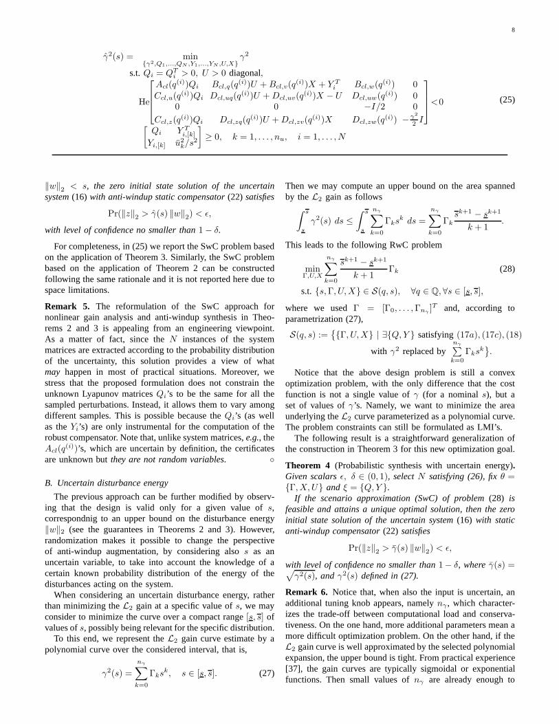
γ2(s) = minγ2,Q1,...,QN ,Y1,...,YN ,U,X

γ2

s.t.Qi = QTi > 0, U > 0 diagonal,

He

Acl(q(i))Qi Bcl,q(q

(i))U +Bcl,v(q(i))X + Y T

i Bcl,w(q(i)) 0

Ccl,u(q(i))Qi Dcl,uq(q

(i))U +Dcl,uv(q(i))X − U Dcl,uw(q

(i)) 00 0 −I/2 0

Ccl,z(q(i))Qi Dcl,zq(q

(i))U +Dcl,zv(q(i))X Dcl,zw(q

(i)) − γ2

2 I

<0

[

Qi Y Ti,[k]

Yi,[k] u2k/s

2

]

≥ 0, k = 1, . . . , nu, i = 1, . . . , N

(25)

‖w‖2 < s, the zero initial state solution of the uncertainsystem(16) with anti-windup static compensator(22) satisfies

Pr(‖z‖2 > γ(s) ‖w‖2) < ǫ,

with level of confidence no smaller than1− δ.

For completeness, in (25) we report the SwC problem basedon the application of Theorem 3. Similarly, the SwC problembased on the application of Theorem 2 can be constructedfollowing the same rationale and it is not reported here due tospace limitations.

Remark 5. The reformulation of the SwC approach fornonlinear gain analysis and anti-windup synthesis in Theo-rems 2 and 3 is appealing from an engineering viewpoint.As a matter of fact, since theN instances of the systemmatrices are extracted according to the probability distributionof the uncertainty, this solution provides a view of whatmay happen in most of practical situations. Moreover, westress that the proposed formulation does not constrain theunknown Lyapunov matricesQi’s to be the same for all thesampled perturbations. Instead, it allows them to vary amongdifferent samples. This is possible because theQi’s (as wellas theYi’s) are only instrumental for the computation of therobust compensator. Note that, unlike system matrices,e.g., theAcl(q

(i))’s, which are uncertain by definition, the certificatesare unknown butthey are not random variables.

B. Uncertain disturbance energy

The previous approach can be further modified by observ-ing that the design is valid only for a given value ofs,correspondnig to an upper bound on the disturbance energy‖w‖2 (see the guarantees in Theorems 2 and 3). However,randomization makes it possible to change the perspectiveof anti-windup augmentation, by considering alsos as anuncertain variable, to take into account the knowledge of acertain known probability distribution of the energy of thedisturbances acting on the system.

When considering an uncertain disturbance energy, ratherthan minimizing theL2 gain at a specific value ofs, we mayconsider to minimize the curve over a compact range[s, s] ofvalues ofs, possibly being relevant for the specific distribution.

To this end, we represent theL2 gain curve estimate by apolynomial curve over the considered interval, that is,

γ2(s) =

nγ∑

k=0

Γksk, s ∈ [s, s]. (27)

Then we may compute an upper bound on the area spannedby theL2 gain as follows

∫ s

s

γ2(s) ds ≤

∫ s

s

nγ∑

k=0

Γksk ds =

nγ∑

k=0

Γk

sk+1 − sk+1

k + 1.

This leads to the following RwC problem

minΓ,U,X

nγ∑

k=0

sk+1 − sk+1

k + 1Γk (28)

s.t. s,Γ, U,X ∈ S(q, s), ∀q ∈ Q, ∀s ∈ [s, s],

where we usedΓ = [Γ0, . . . ,Γnγ]T and, according to

parametrization (27),

S(q, s) :=

Γ, U,X | ∃Q, Y satisfying(17a), (17c), (18)

with γ2 replaced bynγ∑

k=0

Γksk

.

Notice that the above design problem is still a convexoptimization problem, with the only difference that the costfunction is not a single value ofγ (for a nominals), but aset of values ofγ’s. Namely, we want to minimize the areaunderlying theL2 curve parameterized as a polynomial curve.The problem constraints can still be formulated as LMI’s.

The following result is a straightforward generalization ofthe construction in Theorem 3 for this new optimization goal.

Theorem 4 (Probabilistic synthesis with uncertain energy).Given scalarsǫ, δ ∈ (0, 1), selectN satisfying (26), fixθ =Γ, X, U and ξ = Q, Y .

If the scenario approximation (SwC) of problem(28) isfeasible and attains a unique optimal solution, then the zeroinitial state solution of the uncertain system(16) with staticanti-windup compensator(22) satisfies

Pr(‖z‖2 > γ(s) ‖w‖2) < ǫ,

with level of confidence no smaller than1− δ, whereγ(s) =√

γ2(s), andγ2(s) defined in (27).

Remark 6. Notice that, when also the input is uncertain, anadditional tuning knob appears, namelynγ , which character-izes the trade-off between computational load and conserva-tiveness. On the one hand, more additional parameters mean amore difficult optimization problem. On the other hand, if theL2 gain curve is well approximated by the selected polynomialexpansion, the upper bound is tight. From practical experience[37], the gain curves are typically sigmoidal or exponentialfunctions. Then small values ofnγ are already enough to

9

obtain good results (usually, from3 to 6). Notice that otherbasis functions whose integral is linearly parameterized canbe suitably selected, without any conceptual change.

C. Optimized domain of attraction and reachable set

Similar derivations to the ones of the previous sections canbe obtained by focusing on different performance goals, aswell characterized in [12] (see also [24]). In particular, twoperformance goals which have been well characterized withinthe context of the use of generalized sectors for saturatedsystems correspond to: i) maximizing the size of a quadraticestimate of the domain of attraction of the origin in theabsence of disturbances (that is,w = 0), ii) minimizingthe best quadratic estimate of the reachable set from zeroinitial conditions and in the presence of a bounded disturbance‖w‖2 ≤ s.

The goal of this section is then to briefly overview thepossible extensions of the results in Theorems 3 and 4 tothese two cases. The following two propositions establish thebaseline results, proven in [12], [24] for the nominal case.

Proposition 4 (Domain of attraction). Given the plant-controller pair (13), (14) and a matrixQ = QT > 0, considerthe nominal system, that isQ ≡ q is a singleton. Assumethat the SDP problem

maxQ,Q,Y,U,X

log det(Q) (31)

s.t. (29), ∀q ∈ Q,

is feasible. Then, selecting the static anti-windup gain asin(22), the nonlinear algebraic loop in (16) is well posed andfor any initial conditionx(0) in the set

E(Q−1) := x : xT Q−1x ≤ 1, (32)

the (unique) solutionx to the anti-windup closed loop withw = 0 satisfies lim

t→∞|x(t)| = 0.

Proposition 5 (Reachable set). Given the plant-controller pair(13), (14), and a scalars > 0, consider the nominal system,that isQ ≡ q is a singleton. Assume that the SDP problem

minQ,Y,U,X

trace(Q) (33)

s.t. (30), ∀q ∈ Q,

is feasible. Then, selecting the static anti-windup gain asin(22), the nonlinear algebraic loop in (16) is well posed andany solution fromx(0) = 0 with ‖w‖2 ≤ s satisfies

x(t) ∈ E(Q−1) = x : xT Q−1x ≤ 1, ∀t ≥ 0.

In light of the results summarized above, we can formulaterobust optimal design and analysis exploiting the constraints(29) and (30), respectively, and leading to randomized analysisand synthesis tools. These are stated below in two theoremswhose formulations parallel the one of Theorem 3. Analysisresults can also be easily stated, paralleling the formulation inTheorem 2, but are omitted due to their straightforward nature,and to avoid overloading the exposition.

Theorem 5 (Robust domain of attraction). Given scalarsǫ, δ ∈ (0, 1), selectN satisfying (26), fixθ =

Q,X, U

and ξ = Q, Y .If for a selection ofQ = QT > 0 and a scalarα > 0 the

scenario approximation (SwC) of problem(31) is feasible andattains a unique optimal solution, then for any initial conditionin the set (32), any solutionx of the uncertain system(16) withanti-windup static compensator(22) and withw = 0 satisfiesfor all t ≥ 0,

x(0) ∈ E(Q−1) ⇒ Pr(

limt→∞

|x(t)| = 0)

≥ 1− ǫ,

with level of confidence no smaller than1− δ.

In Theorem 5 we characterize properties of the scenarioapproximation (SwC) of problem (31) with the certificatesξ = Q, Y . Then, according to the definition in (5), itbecomes clear that constraints (29) are imposed with certifi-catesQ, Y depending on the uncertaintyq, which lead toreduced conservativeness. An interesting feature arisingfromtheseq-dependent certificates in (29) is that the rightmostconstraint in (29a) implies thatQ is a uniform lower boundon all certificatesQi. Stated otherwise, this implies thatE(Q−1) ⊂ E(Q−1

i ), i = 1, . . . , N , namely setE(Q−1)is a subset of all the stability regionsE(Q−1

i ) obtained foreach one of the extracted samplesqi. Then, differently fromclassical deterministic approaches, although the setE(Q−1)is a guaranteed region of robust stability, it is not necessarilya forward invariant set (whereas for eachqi we know thatE(Q−1

i ) is a forward invariant set).A similar (but somewhat converse) comment applies to the

robust reachable set studied in the theorem below, wherein therightmost inequality in (30a) implies that for eachqi we haveE(s2Q−1

i ) ⊂ E(Q−1), i = 1, . . . , N , namely setE(Q−1) isa superset of all the reachable set estimatesE(s2Q−1

i ) obtainedfrom the scenario approximation of (33).

Theorem 6 (Robust reachable set). Given scalarss > 0, andǫ, δ ∈ (0, 1), selectN satisfying (26), fixθ =

Q,X, U

andξ = Q, Y .

If the scenario approximation (SwC) of problem(33) isfeasible and attains a unique optimal solution, then for each‖w‖2 < s, the zero initial state solution of the uncertainsystem(16) with anti-windup static compensator(22) satisfies

Pr(

x(t) /∈ E(Q−1))

< ǫ

for all t ≥ 0, with level of confidence no smaller than1− δ.

Remark 7. Notice that Theorem 6 proposes a selection ofthe anti-windup gain that minimizes a suitable measure of thesize of the reachable set for a specific selection of the bounds on theL2 norm of the disturbancew. It is then possible tofollow similar derivations to those given in Section III-B withthe goal of providing a suitably weighted optimal selectionof the anti-windup gain performed by focusing on the sizeof the reachable set in the presence of an unknownL2

norm of the disturbance, for which probabilistic information isavailable. Then one may quantify the “size” of the reachableset for each value ofs by a suitable parametrization similarto the right hand side of (27), and finally minimize some net

10

Q = QT > 0, U > 0 diagonal, Q ≤ Q, (29a)

He

[

Acl(q)Q Bcl,q(q) +Bcl,v(q)XCcl,u(q)Q− Y Dcl,uq(q)U +Dcl,uv(q)X − U

]

< 0, (29b)[

u2k Y[k]

Y T[k] Q

]

≥ 0, k = 1, . . . , nu, (29c)

Q = QT > 0, U > 0 diagonal, s2Q ≥ Q, (30a)

He

Acl(q)Q Bcl,q(q) +Bcl,v(q)X Bcl,w(q)Ccl,u(q)Q− Y Dcl,uq(q)U +Dcl,uv(q)X − U Dcl,uw(q)

0 0 −I/2

< 0, (30b)

[

u2k/s

2 Y[k]

Y T[k] Q

]

≥ 0, k = 1, . . . , nu, (30c)

performance metric taking into account the whole range ofpossible occurrences of theL2 norm s of the disturbancew.Since this extension is straightforward, it is not discussed ingreater detail.

IV. SIMULATION EXAMPLES

The following numerical results are obtained using MatlabR2015a on a 64 bit Windows 8.1 computer equipped withan Intel(R) Core(TM) i7-4500U at 1.80 GHz and 8 GB ofmemory. The optimization is implemented using Yalmip [25]and Sedumi [32].

A. L2 gain minimization

In this section, we show the effectiveness of the proposedapproach, by designing an anti-windup compensator for thepassive electrical network in Fig. 1. The circuit is a bench-mark example in the anti-windup literature and was alreadyemployed in [37] to show the potential of static anti-windupin a deterministic context.

Vi Vo

C2

C3

C1

R2 R4

kR5R3R1

Fig. 1. The passive electrical network with saturated inputvoltage.

The dynamics of the network is determined by 5 resistorsand 3 capacitors, whose nominal values are reported in TableI.The gaink is instead selected such that the transfer functionbetweenVi andVo is monic.

After some cumbersome computations, the transfer functionof the network turns out to be

G(s) =s2 + C1R2+C2R4

C1C2R2R4s+ 1

C1C2R2R4

s3 + η2

η3

s2 + η1

η3

s+ 1η3

(34)

name value unitsR1 313 Ω

R2 20 Ω

R3 315 Ω

R4 17 Ω

R5 10 Ω

C1 0.01 F

C2 0.01 F

C3 0.01 F

TABLE INOMINAL PARAMETER VALUES FOR THE NETWORK INFIG. 1.

with

η1 = C1R1 + C1R2 + C2R3 + C2R4 + C3R5, (35)

η2 = C1C2R1R3 + C1C2R1R4 + C1C2R2R3

+ C1C2R2R4 + C1C3R1R5 + C1C3R2R5

+ C2C3R3R5 + C2C3R4R5, (36)

η3 = C1C2C3R1R3R5 + C1C2C3R1R4R5

+ C1C2C3R2R3R5 + C1C2C3R2R4R5. (37)

Notice that the dependence ofηi, i = 1, 2, 3 upon the physicalparameters is highly nonlinear.

The nominal plant can then be put in the form (13) viasuitable state-space realization, where

[

Ap Bp,u Bp,w

Cp,z Dp,zu Dp,zw

Cp,y Dp,yu Dp,yw

]

=

−10.6 −6.09 −0.9 1 0

1 0 0 0 0

0 1 0 0 0

−1 −11 −30 0 0

1 11 30 0 0

,

andw represents the reference value for the output voltageVo,so thatz = w − y is the tracking error.

The controller is a PID and it is designed based on thenominal model, such that the nominal phase margin is89.5degrees and the nominal gain margin is infinity. In the form(14), the controller is expressed by the matrices

[

Ac Bc,y Bc,w

Cc Dc,y Dc,w

]

=

−80 0 1 −11 0 0 0

20.25 1600 80 −80

.

11

Assume now that the inputVi is saturated between theminimum and the maximum voltages±1. For a specificvalue of s, a static anti-windup compensator based on thenominal model can be designed to minimize the nonlineargain between the reference and the tracking error, by solvingthe optimization problem (21) and relying on Proposition 3.Using s = 0.003, the nominaloptimal valueγ2

n(s) = 2.31 isobtained, together with the optimal nominal anti-windup gainDnom

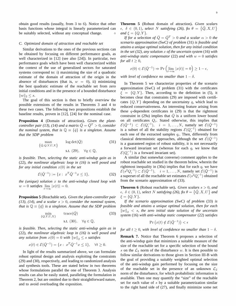
aw = [−0.0855, 0.0011, 0.9887]T. This value correspondsto the squared value of the dashed blue curve in Fig. 2 at theabscissas = 0.003 ≈ 10−2.52.

Under the hypothesis that the parameters are Gaussian dis-tributed with mean values as in Table I and standard deviationof 10%, a robust randomized compensator can be computedfollowing Theorem 3. First notice thatnθ = 5 = 1+3+1 (aris-ing from γ2, X andU , respectively). Then, fixing parametersε = 0.01 and δ = 10−6, we see thatN = 2819 samples arenecessary to satisfy (4). Therefore, we follow the sequentialalgorithm of Section II-C to reduce the computational burden.In particular, using the same values = 0.003 as in the nominalsynthesis above, we apply the Sequential algorithm for SwC,initialized with kt = 10. Such a procedure terminates after3 iterations, using onlyN = 846 samples, and providingthe robust optimal valueγ2

r = 9.1 (evidently larger thanthe nominal one), together with the optimal robust anti-windup gainDrand

aw = [−2.1493, 0.0266, 0.6407]T. This valueapproximately corresponds to the squared value of the solidred curve in Fig. 2 at the abscissas = 0.003 ≈ 10−2.52.We observe a slight difference between the two values (inthe figure, the gain is higher), justified by the fact that theperformance analysis is carried out with a different set ofsamples. We should remark that in terms of computationaltime, the SwC approach is more demanding than the nominaldesign. In this example, the elapsed time for compensatordesign is approximately7 seconds in the latter case and about5 hours in the former.

s×10-3

2 2.5 3 3.5 4 4.5 5 5.5

γ

0

5

10

15

20

25

30

35

no AW (robust analysis)

no AW (nominal analysis)

nAW (robust analysis)

nAW (nominal analysis)

rAW (robust analysis)

rAW (nominal analysis)

Fig. 2. L2 gain estimates for the nonlinear closed-loop systems with andwithout anti-windup compensator. Both robust (solid) and nominal (dashed)analysis are considered to assess the performance of robust(blue, Drand

aw )and nominal (red,Dnom

aw ) compensators with respect to the system withoutanti-windup augmentation (black).

Once the nominal and the robust anti-windup gains arefixed, we may characterize their nominal and robust perfor-mance by applying, respectively, the analysis tools of Propo-sition 2 and Theorem 2. For comparison purposes, we studythe nominal and robust performance also for the case withno anti-windup compensation. Comprehensively, we obtain sixcurves, all reported in Fig. 2, where the nominal curves aredashed and the robust ones are solid.

As expected, we observe that the robust compensator out-performs the one designed for the nominal system, as far as therobustL2 gain is concerned (solid curves). Conversely, whenthe performance is evaluated on the nominal system (dashedcurves), the robust compensator yields worse results, since itis more conservative. From the analysis point of view, noticealso that theL2 gains estimated using the robust probabilisticmethod are larger than the ones given by the nominal analysis.This holds for any configuration of the saturated closed-loopsystem (without anti-windup, with nominal compensator andwith robust compensator).

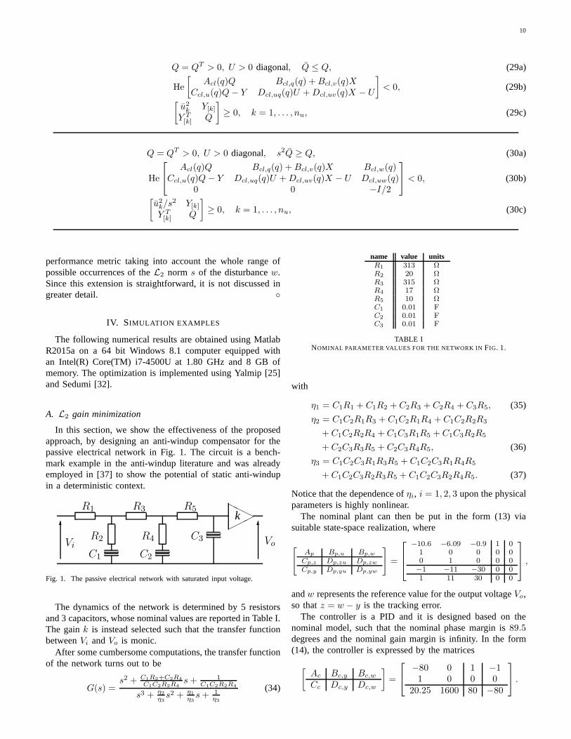
The time-domain performance degradation of the nominalclosed-loop system using the robust compensator in placeof the nominal one can be assessed by looking at the timeresponses illustrated in Fig. 3. From the figure, we concludethat, although in any case the use of a compensator (redsolid and blue dash-dotted curves) improves upon the responsewithout anti-windup (black dotted) in terms of tracking errorand overshoot, we have to accept worse behavior in nominalconditions when using robust anti-windup (indeed, the bluedash-dotted response yields faster transients than the redsolidcurves). However, this choice is rewarding when acting on a

0 5 10 15 20 25

−2

−1

0

1

2

Time [−]

unconno AWnAWrAW

Fig. 3. Time responses of the closed-loop system with nominal parametersand different configurations of the anti-windup architecture: unconstrainedsystem (dashed), saturated system without anti-windup compensator (dotted),saturated system with nominal anti-windupDnom

aw (dash-dotted) and saturatedsystem with robust anti-windupDrand

aw (solid).

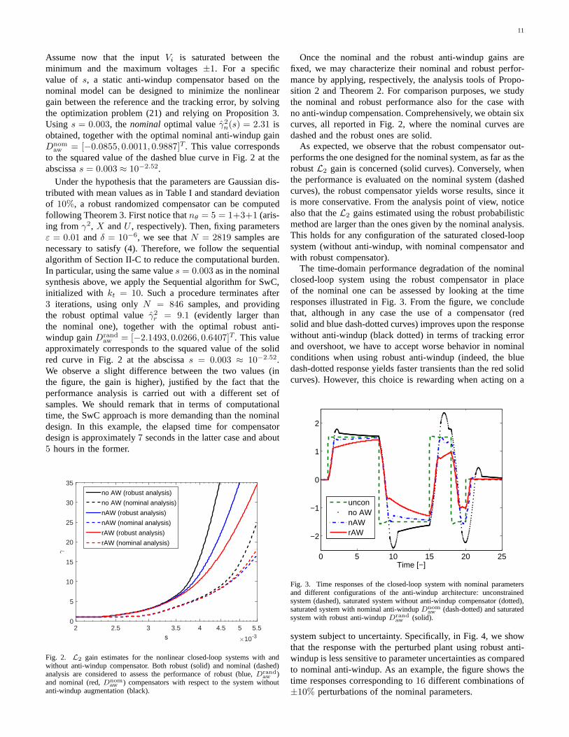
system subject to uncertainty. Specifically, in Fig. 4, we showthat the response with the perturbed plant using robust anti-windup is less sensitive to parameter uncertainties as comparedto nominal anti-windup. As an example, the figure shows thetime responses corresponding to16 different combinations of±10% perturbations of the nominal parameters.

12

0 10 20−4

−2

0

2

4unconstrained

0 10 20−4

−2

0

2

4no AW

0 10 20−4

−2

0

2

4nominal AW

Time [−]0 10 20

−4

−2

0

2

4randomized AW

Time [−]

Fig. 4. Sixteen perturbed time responses of the uncertain closed-loopsystem with different configurations of the anti-windup architecture: uncon-strained system (upper-left), saturated system without anti-windup compen-sator (upper-right), saturated system with nominal anti-windup Dnom

aw (lowerleft) and saturated system with robust anti-windupDrand

aw (lower right).

It should be here remarked that, if the approach in [16]is employed, the optimization problem for the design of theanti-windup compensator becomes infeasible. This is due tothe conservativeness of the formulation in [16], which requiresa single Lyapunov function for all the possible uncertaininstances of the system.

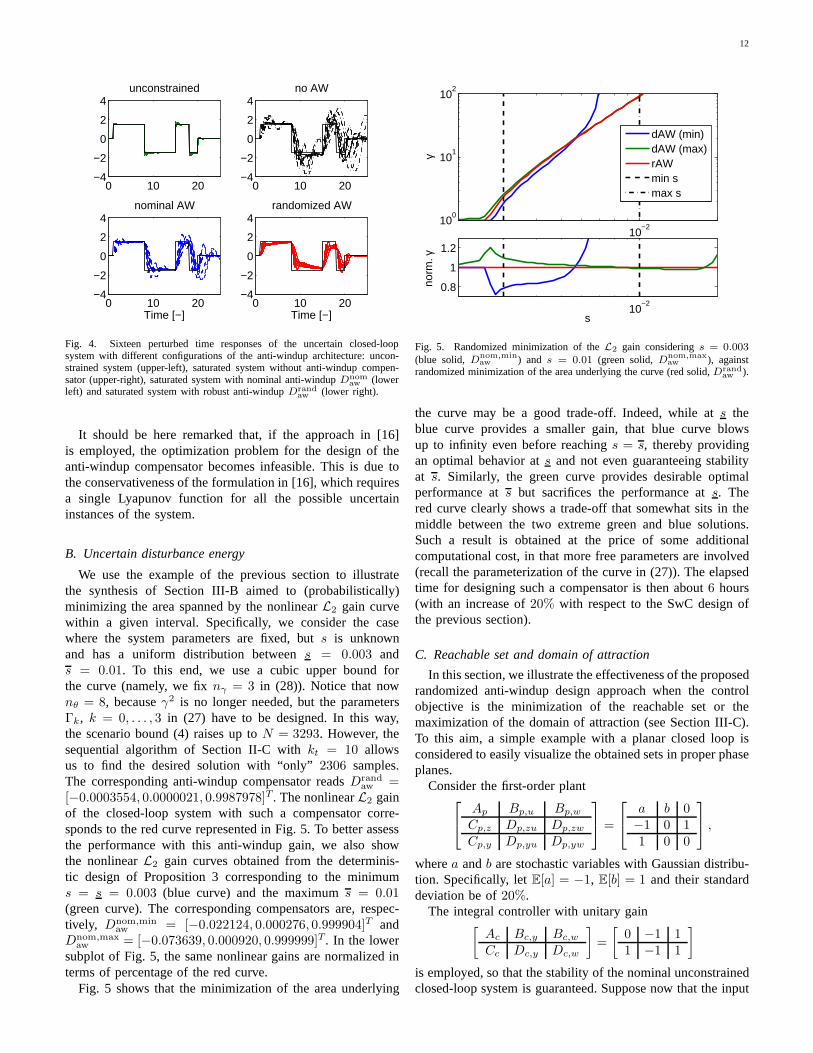
B. Uncertain disturbance energy

We use the example of the previous section to illustratethe synthesis of Section III-B aimed to (probabilistically)minimizing the area spanned by the nonlinearL2 gain curvewithin a given interval. Specifically, we consider the casewhere the system parameters are fixed, buts is unknownand has a uniform distribution betweens = 0.003 ands = 0.01. To this end, we use a cubic upper bound forthe curve (namely, we fixnγ = 3 in (28)). Notice that nownθ = 8, becauseγ2 is no longer needed, but the parametersΓk, k = 0, . . . , 3 in (27) have to be designed. In this way,the scenario bound (4) raises up toN = 3293. However, thesequential algorithm of Section II-C withkt = 10 allowsus to find the desired solution with “only”2306 samples.The corresponding anti-windup compensator readsDrand

aw =[−0.0003554, 0.0000021, 0.9987978]T. The nonlinearL2 gainof the closed-loop system with such a compensator corre-sponds to the red curve represented in Fig. 5. To better assessthe performance with this anti-windup gain, we also showthe nonlinearL2 gain curves obtained from the determinis-tic design of Proposition 3 corresponding to the minimums = s = 0.003 (blue curve) and the maximums = 0.01(green curve). The corresponding compensators are, respec-tively, Dnom,min

aw = [−0.022124, 0.000276, 0.999904]T andDnom,max

aw = [−0.073639, 0.000920, 0.999999]T. In the lowersubplot of Fig. 5, the same nonlinear gains are normalized interms of percentage of the red curve.

Fig. 5 shows that the minimization of the area underlying

10−2

100

101

102

γ

10−2

0.8

1

1.2

s

norm

. γ

dAW (min)dAW (max)rAWmin smax s

Fig. 5. Randomized minimization of theL2 gain considerings = 0.003

(blue solid, Dnom,minaw ) and s = 0.01 (green solid,Dnom,max

aw ), againstrandomized minimization of the area underlying the curve (red solid,Drand

aw ).

the curve may be a good trade-off. Indeed, while ats theblue curve provides a smaller gain, that blue curve blowsup to infinity even before reachings = s, thereby providingan optimal behavior ats and not even guaranteeing stabilityat s. Similarly, the green curve provides desirable optimalperformance ats but sacrifices the performance ats. Thered curve clearly shows a trade-off that somewhat sits in themiddle between the two extreme green and blue solutions.Such a result is obtained at the price of some additionalcomputational cost, in that more free parameters are involved(recall the parameterization of the curve in (27)). The elapsedtime for designing such a compensator is then about6 hours(with an increase of20% with respect to the SwC design ofthe previous section).

C. Reachable set and domain of attraction

In this section, we illustrate the effectiveness of the proposedrandomized anti-windup design approach when the controlobjective is the minimization of the reachable set or themaximization of the domain of attraction (see Section III-C).To this aim, a simple example with a planar closed loop isconsidered to easily visualize the obtained sets in proper phaseplanes.

Consider the first-order plant

Ap Bp,u Bp,w

Cp,z Dp,zu Dp,zw

Cp,y Dp,yu Dp,yw

=

a b 0−1 0 11 0 0

,

wherea andb are stochastic variables with Gaussian distribu-tion. Specifically, letE[a] = −1, E[b] = 1 and their standarddeviation be of20%.

The integral controller with unitary gain[

Ac Bc,y Bc,w

Cc Dc,y Dc,w

]

=

[

0 −1 11 −1 1

]

is employed, so that the stability of the nominal unconstrainedclosed-loop system is guaranteed. Suppose now that the input

13

−1 −0.5 0 0.5 1−1.5

−1

−0.5

0

0.5

1

1.5

xp

x c

(a)

−1 −0.5 0 0.5 1−1.5

−1

−0.5

0

0.5

1

1.5

xp

x c

(b)

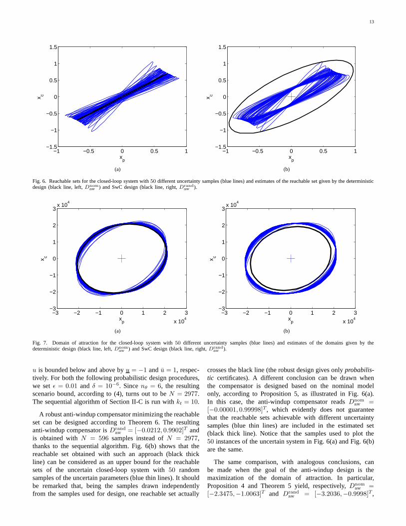
Fig. 6. Reachable sets for the closed-loop system with50 different uncertainty samples (blue lines) and estimates of the reachable set given by the deterministicdesign (black line, left,Dnom

aw ) and SwC design (black line, right,Drandaw ).

−3 −2 −1 0 1 2 3

x 104

−3

−2

−1

0

1

2

3x 10

4

xp

x c

(a)

−3 −2 −1 0 1 2 3

x 104

−3

−2

−1

0

1

2

3x 10

4

xp

x c

(b)

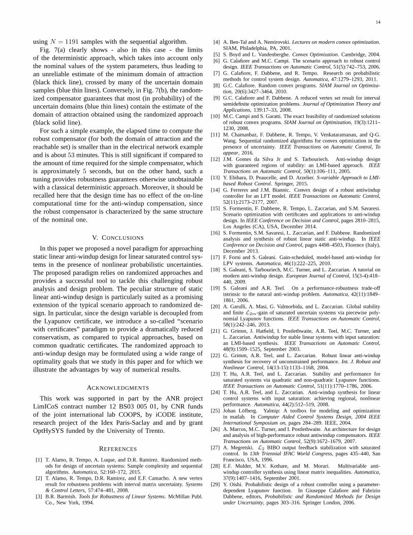
Fig. 7. Domain of attraction for the closed-loop system with50 different uncertainty samples (blue lines) and estimates of the domains given by thedeterministic design (black line, left,Dnom

aw ) and SwC design (black line, right,Drandaw ).

u is bounded below and above byu = −1 andu = 1, respec-tively. For both the following probabilistic design procedures,we setǫ = 0.01 and δ = 10−6. Sincenθ = 6, the resultingscenario bound, according to (4), turns out to beN = 2977.The sequential algorithm of Section II-C is run withkt = 10.

A robust anti-windup compensator minimizing the reachableset can be designed according to Theorem 6. The resultinganti-windup compensator isDrand

aw = [−0.0212, 0.9902]T andis obtained withN = 596 samples instead ofN = 2977,thanks to the sequential algorithm. Fig. 6(b) shows that thereachable set obtained with such an approach (black thickline) can be considered as an upper bound for the reachablesets of the uncertain closed-loop system with50 randomsamples of the uncertain parameters (blue thin lines). It shouldbe remarked that, being the samples drawn independentlyfrom the samples used for design, one reachable set actually

crosses the black line (the robust design gives onlyprobabilis-tic certificates). A different conclusion can be drawn whenthe compensator is designed based on the nominal modelonly, according to Proposition 5, as illustrated in Fig. 6(a).In this case, the anti-windup compensator readsDnom

aw =[−0.00001, 0.99998]T, which evidently does not guaranteethat the reachable sets achievable with different uncertaintysamples (blue thin lines) are included in the estimated set(black thick line). Notice that the samples used to plot the50 instances of the uncertain system in Fig. 6(a) and Fig. 6(b)are the same.

The same comparison, with analogous conclusions, canbe made when the goal of the anti-windup design is themaximization of the domain of attraction. In particular,Proposition 4 and Theorem 5 yield, respectively,Dnom

aw =[−2.3475,−1.0063]T and Drand

aw = [−3.2036,−0.9998]T ,

14

usingN = 1191 samples with the sequential algorithm.Fig. 7(a) clearly shows - also in this case - the limits

of the deterministic approach, which takes into account onlythe nominal values of the system parameters, thus leading toan unreliable estimate of the minimum domain of attraction(black thick line), crossed by many of the uncertain domainsamples (blue thin lines). Conversely, in Fig. 7(b), the random-ized compensator guarantees that most (in probability) of theuncertain domains (blue thin lines) contain the estimate ofthedomain of attraction obtained using the randomized approach(black solid line).

For such a simple example, the elapsed time to compute therobust compensator (for both the domain of attraction and thereachable set) is smaller than in the electrical network exampleand is about53 minutes. This is still significant if compared tothe amount of time required for the simple compensator, whichis approximately5 seconds, but on the other hand, such atuning provides robustness guarantees otherwise unobtainablewith a classical deterministic approach. Moreover, it should berecalled here that the design time has no effect of the on-linecomputational time for the anti-windup compensation, sincethe robust compensator is characterized by the same structureof the nominal one.

V. CONCLUSIONS

In this paper we proposed a novel paradigm for approachingstatic linear anti-windup design for linear saturated control sys-tems in the presence of nonlinear probabilistic uncertainties.The proposed paradigm relies on randomized approaches andprovides a successful tool to tackle this challenging robustanalysis and design problem. The peculiar structure of staticlinear anti-windup design is particularly suited as a promisingextension of the typical scenario approach to randomized de-sign. In particular, since the design variable is decoupledfromthe Lyapunov certificate, we introduce a so-called “scenariowith certificates” paradigm to provide a dramatically reducedconservatism, as compared to typical approaches, based oncommon quadratic certificates. The randomized approach toanti-windup design may be formulated using a wide range ofoptimality goals that we study in this paper and for which weillustrate the advantages by way of numerical results.

ACKNOWLEDGMENTS

This work was supported in part by the ANR projectLimICoS contract number 12 BS03 005 01, by CNR fundsof the joint international lab COOPS, by iCODE institute,research project of the Idex Paris-Saclay and and by grantOptHySYS funded by the University of Trento.

REFERENCES

[1] T. Alamo, R. Tempo, A. Luque, and D.R. Ramirez. Randomized meth-ods for design of uncertain systems: Sample complexity and sequentialalgorithms.Automatica, 52:160–172, 2015.

[2] T. Alamo, R. Tempo, D.R. Ramirez, and E.F. Camacho. A new vertexresult for robustness problems with interval matrix uncertainty. Systems& Control Letters, 57:474–481, 2008.

[3] B.R. Barmish.Tools for Robustness of Linear Systems. McMillan Publ.Co., New York, 1994.

[4] A. Ben-Tal and A. Nemirovski.Lectures on modern convex optimization.SIAM, Philadelphia, PA, 2001.

[5] S. Boyd and L. Vandenberghe.Convex Optimization. Cambridge, 2004.[6] G. Calafiore and M.C. Campi. The scenario approach to robust control

design.IEEE Transactions on Automatic Control, 51(5):742–753, 2006.[7] G. Calafiore, F. Dabbene, and R. Tempo. Research on probabilistic

methods for control system design.Automatica, 47:1279–1293, 2011.[8] G.C. Calafiore. Random convex programs.SIAM Journal on Optimiza-

tion, 20(6):3427–3464, 2010.[9] G.C. Calafiore and F. Dabbene. A reduced vertex set resultfor interval

semidefinite optimization problems.Journal of Optimization Theory andApplications, 139:17–33, 2008.

[10] M.C. Campi and S. Garatti. The exact feasibility of randomized solutionsof robust convex programs.SIAM Journal on Optimization, 19(3):1211–1230, 2008.

[11] M. Chamanbaz, F. Dabbene, R. Tempo, V. Venkataramanan,and Q-G.Wang. Sequential randomized algorithms for convex optimization in thepresence of uncertainty.IEEE Transactions on Automatic Control, Toappear, 2016.

[12] J.M. Gomes da Silva Jr and S. Tarbouriech. Anti-windup designwith guaranteed regions of stability: an LMI-based approach. IEEETransactions on Automatic Control, 50(1):106–111, 2005.

[13] Y. Ebihara, D. Peaucelle, and D. Arzelier.S-variable Approach to LMI-based Robust Control. Springer, 2015.

[14] G. Ferreres and J.M. Biannic. Convex design of a robust antiwindupcontroller for an LFT model.IEEE Transactions on Automatic Control,52(11):2173–2177, 2007.

[15] S. Formentin, F. Dabbene, R. Tempo, L. Zaccarian, and S.M. Savaresi.Scenario optimization with certificates and applications to anti-windupdesign. InIEEE Conference on Decision and Control, pages 2810–2815,Los Angeles (CA), USA, December 2014.

[16] S. Formentin, S.M. Savaresi, L. Zaccarian, and F. Dabbene. Randomizedanalysis and synthesis of robust linear static anti-windup. In IEEEConference on Decision and Control, pages 4498–4503, Florence (Italy),December 2013.

[17] F. Forni and S. Galeani. Gain-scheduled, model-based anti-windup forLPV systems.Automatica, 46(1):222–225, 2010.

[18] S. Galeani, S. Tarbouriech, M.C. Turner, and L. Zaccarian. A tutorial onmodern anti-windup design.European Journal of Control, 15(3-4):418–440, 2009.

[19] S. Galeani and A.R. Teel. On a performance-robustness trade-offintrinsic to the natural anti-windup problem.Automatica, 42(11):1849–1861, 2006.

[20] A. Garulli, A. Masi, G. Valmorbida, and L. Zaccarian. Global stabilityand finiteL2m-gain of saturated uncertain systems via piecewise poly-nomial Lyapunov functions.IEEE Transactions on Automatic Control,58(1):242–246, 2013.

[21] G. Grimm, J. Hatfield, I. Postlethwaite, A.R. Teel, M.C.Turner, andL. Zaccarian. Antiwindup for stable linear systems with input saturation:an LMI-based synthesis.IEEE Transactions on Automatic Control,48(9):1509–1525, September 2003.

[22] G. Grimm, A.R. Teel, and L. Zaccarian. Robust linear anti-windupsynthesis for recovery of unconstrained performance.Int. J. Robust andNonlinear Control, 14(13-15):1133–1168, 2004.

[23] T. Hu, A.R. Teel, and L. Zaccarian. Stability and performance forsaturated systems via quadratic and non-quadratic Lyapunov functions.IEEE Transactions on Automatic Control, 51(11):1770–1786, 2006.

[24] T. Hu, A.R. Teel, and L. Zaccarian. Anti-windup synthesis for linearcontrol systems with input saturation: achieving regional, nonlinearperformance.Automatica, 44(2):512–519, 2008.

[25] Johan Lofberg. Yalmip: A toolbox for modeling and optimizationin matlab. In Computer Aided Control Systems Design, 2004 IEEEInternational Symposium on, pages 284–289. IEEE, 2004.

[26] A. Marcos, M.C. Turner, and I. Postlethwaite. An architecture for designand analysis of high-performance robust antiwindup compensators.IEEETransactions on Automatic Control, 52(9):1672–1679, 2007.

[27] A. Megretski. L2 BIBO output feedback stabilization with saturatedcontrol. In 13th Triennial IFAC World Congress, pages 435–440, SanFrancisco, USA, 1996.

[28] E.F. Mulder, M.V. Kothare, and M. Morari. Multivariable anti-windup controller synthesis using linear matrix inequalities. Automatica,37(9):1407–1416, September 2001.

[29] Y. Oishi. Probabilistic design of a robust controller using a parameter-dependent Lyapunov function. In Giuseppe Calafiore and FabrizioDabbene, editors,Probabilistic and Randomized Methods for Designunder Uncertainty, pages 303–316. Springer London, 2006.

15

[30] I. Postlethwaite, M.C. Turner, and G. Herrmann. Robustcontrolapplications.Annual Reviews in Control, 31(1):27–39, 2007.

[31] J. Sofrony, M.C. Turner, and I. Postlethwaite. Anti-windup synthesisusing Riccati equations.International Journal of Control, 80(1):112–128, 2007.

[32] J.F. Sturm. Using SeDuMi 1.02, a MATLAB toolbox for optimizationover symmetric cones.Optimization methods and software, 11(1-4):625–653, 1999.

[33] S. Tarbouriech, G. Garcia, J.M. Gomes da Silva Jr., and I. Queinnec.Stability and stabilization of linear systems with saturating actuators.Springer-Verlag London Ltd., 2011.

[34] S. Tarbouriech and M. Turner. Anti-windup design: an overview ofsome recent advances and open problems.IET Proc. Control Theory &Applications, 3(1):1–19, 2009.

[35] R. Tempo, G.C. Calafiore, and F. Dabbene.Randomized Algorithms forAnalysis and Control of Uncertain Systems: With Applications. Springer,2nd edition, 2013.

[36] M.C. Turner, G. Herrmann, and I. Postlethwaite. Incorporating ro-bustness requirements into antiwindup design.IEEE Transactions onAutomatic Control, 52(10):1842–1855, 2007.

[37] L. Zaccarian and A.R. Teel.Modern anti-windup synthesis: controlaugmentation for actuator saturation. Princeton University Press,Princeton (NJ), 2011.