robust global ocean cooling trend for the...

Citation: McGregor, Helen, Evans, Michael, Goosse, Hugues, Leduc, Guillaume, Martrat, Belen, Addison, Jason, Mortyn, Graham, Oppo, Delia, Seidenkrantz, Marit-Solveig, Sicre, Marie-Alexandrine, Phipps, Steven, Selvaraj, Kandasamy, Thirumalai, Kaustubh, Filipsson, Helena and Ersek, Vasile (2015) Robust global ocean cooling trend for the pre-industrial Common Era. Nature Geoscience, 8 (9). pp. 671-677. ISSN 1752-0894

Published by: Nature Publishing

URL: http://dx.doi.org/10.1038/ngeo2510 <http://dx.doi.org/10.1038/ngeo2510>

This version was downloaded from Northumbria Research Link: http://nrl.northumbria.ac.uk/23465/

Northumbria University has developed Northumbria Research Link (NRL) to enable users to access the University’s research output. Copyright © and moral rights for items on NRL are retained by the individual author(s) and/or other copyright owners. Single copies of full items can be reproduced, displayed or performed, and given to third parties in any format or medium for personal research or study, educational, or not-for-profit purposes without prior permission or charge, provided the authors, title and full bibliographic details are given, as well as a hyperlink and/or URL to the original metadata page. The content must not be changed in any way. Full items must not be sold commercially in any format or medium without formal permission of the copyright holder. The full policy is available online: http://nrl.northumbria.ac.uk/policies.html

This document may differ from the final, published version of the research and has been made available online in accordance with publisher policies. To read and/or cite from the published version of the research, please visit the publisher’s website (a subscription may be required.)

http://nrl.northumbria.ac.uk/policies.html

1

Robust global ocean cooling trend for the pre-industrial Common Era

Supplementary Information

Helen V. McGregor*, Michael N. Evans, Hugues Goosse, Guillaume Leduc, Belen Martrat, Jason A. Addison, P. Graham Mortyn, Delia W. Oppo, Marit-Solveig Seidenkrantz, Marie-

Alexandrine Sicre, Steven J. Phipps, Kandasamy Selvaraj , Kaustubh Thirumalai, Helena L. Filipsson, and Vasile Ersek

*Corresponding author: H. V. McGregor, School of Earth and Environmental Sciences, University of Wollongong, Northfields Ave, NSW 2522, Australia. Email: [email protected] Telephone: +61 432 897 139

2

Table of contents Metadatabase acknowledgments (continued from main text) .............................. 3

Section 1: Additional methods on Ocean2k SST synthesis selection criteria .... 4 SST reconstructions and calibrations ........................................................................... 13 Age model criteria ............................................................................................................ 13 Special cases – multiple SST estimates ........................................................................ 14 Reconstructions from upwelling regions ...................................................................... 16

Section 2: Additional methods on the CSIRO Mk3L cumulative forcing, and LOVECLIM single forcing, model simulations ...................................................... 18

Section 3: Binning ................................................................................................... 20

Section 4: Standardization ..................................................................................... 21 Alternatives to standardization: Calibration of the Ocean2k SST synthesis ............. 21 Are estimates of the linear cooling trend dependent on standardization? ................ 25

A note on paleoclimate data and model simulation anomaly SST trend amplitudes ...... 26

Section 5: Testing if the Ocean2k synthesis network is representative of global SST on 200-year time scales .................................................................................. 29

Methods for correlation map in Figure 1 ....................................................................... 29 Weighting the SST synthesis for ocean basin area ...................................................... 31

Section 6: Sensitivity tests ..................................................................................... 33 Sources of bias and error in SST reconstructions ....................................................... 33

C37 alkenones unsaturation index ................................................................................. 33 Mg/Ca in foraminifera ..................................................................................................... 34 TEX86 .............................................................................................................................. 35 Sr/Ca in coral .................................................................................................................. 36 Dinoflagellate cysts ......................................................................................................... 36 Planktic foraminifera ....................................................................................................... 37 Generic sources of bias and error .................................................................................. 38

Additional testing for possible bias due to proximity to coasts ................................. 39 Supplementary Figure S9: Spatial distribution of reconstruction categories ........... 40

Section 7: Calculation of bin-to-bin changes ....................................................... 44

Section 8: 20th century SST trends ........................................................................ 45

Section 9: Paleoclimate data and model simulation comparison ...................... 49 Method for constructing the Terrestrial 2k composite ................................................. 49 Supplementary Table S14: Paleoclimate data and model simulation trend statistics ........................................................................................................................................... 50 Supplementary Figure S11: Single and cumulative forcing simulation plots ............ 51

Section 10: Energy Balance Model methods ........................................................ 52

Section 11: Volcanic forcing and LOVECLIM and CSIRO Mk3L model simulations .............................................................................................................. 53

Section 12: Supplementary References ................................................................ 55

3

Metadatabase acknowledgments (continued from main text)

We thank the following volunteers who kindly gave their time and effort to help us compile the PAGES Ocean2k metadatabase, from which the datasets used in this study were selected.

Basanta Raj Adhikari Ally May M. Waseem Ashiq David McCarthy William Austin Arto Miettinen David Black Paola Moffa Sanchez Patrick Blaser Colin Mustaphi Sean P. Bryan Alessandra Negri Rodrigo Abarca del Río Sena Akçer Ön M. Carmen Alvarez-Castro Juan F. Paniagua Will Carpenter Grace Park Ziying Chu Genna Patton Daniele Colombaroli Maria Serena Poli Stephen Cullen Irina Polovodova Laura Cunningham John Rogers Carin Andersson Dahl Marta Rufino Maxime Debret Netramani Sagar Erin Delman Casey Saenger Kristine DeLong Katherine Selby Femke Davids Sudhir Raj Shrestha Anuar El Ouahabi Triranta Sircar Katherine Esswein Samantha Stevenson Mary Evans Jessica Tierney Kelly Gibson Manish Tiwari Cyril Giry Ko Hiu Tung Joan O. Grimalt Amy J. Wagner Ben Horton Alan D. Wanamaker Jr. Helga Bára Bartels Jónsdóttir Coco Wang Flavio Justino Colleen Wilson Kinuyo Kanamaru Henry Wu Giri Kattel Richard Wylde Thorsten Kiefer Hong Yan Kelly H. Kilbourne Andrew William Kingston Karen Kohfield Mahjoor Ahmad Lone Sultan Mahamud

4

Section 1: Additional methods on Ocean2k SST synthesis selection criteria

A total of 57 published reconstructions comprise the Ocean2k SST synthesis (Supplementary Table S1; Supplementary Figure S1). The reconstructions were selected from the Ocean2k metadatabase (http://www.pages-igbp.org/workinggroups/ocean2k/data) The metadatabase was assembled in 2011-2012 and has been updated periodically since then. The cutoff for inclusion in the present synthesis was May 2013. The reconstructions met the following key selection criteria that:

1. The data were from a marine archive (e.g. corals, marine sediments).

2. The minimum average sample resolution for each reconstruction was at least one observation every 200 years (centennial).

3. The peer-reviewed, published data were archived in a publically available data repository, primarily PANGAEA (http://www.pangaea.de/) or WDC-paleoclimatology (http://www.ncdc.noaa.gov).

4. The time series was a SST reconstruction (see below for additional calibration details).

5. The reconstruction had at least two age dates between 200 BCE and present (see below for dating additional details).

6. The reconstruction contained data that spanned at least two consecutive bins.

7. The Ocean2k SST synthesis is based on reconstructions that are not used for the Ocean2k ‘High Resolution’ synthesis (Tierney et al., 2015), to ensure data independence for the two synthesis efforts. The ‘High Resolution’ synthesis focuses on annual or higher resolution coral reconstructions, which generally span only the past few centuries.

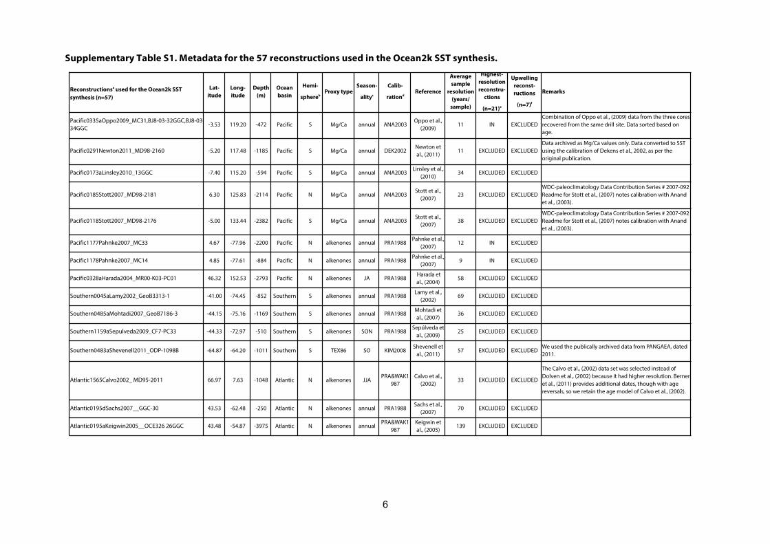
Comments on individual reconstructions and special cases are documented below, and in Supplementary Table S1, along with core location, reconstruction type, calibration, any reported seasonal bias, age dating number and type, and citation for the original publication. Supplementary Table S2 gives the data sources. Supplementary Figure S1 presents the reconstructions. The Ocean2k SST synthesis data matrix is available at: http://www.ncdc.noaa.gov/paleo/study/18718.

5

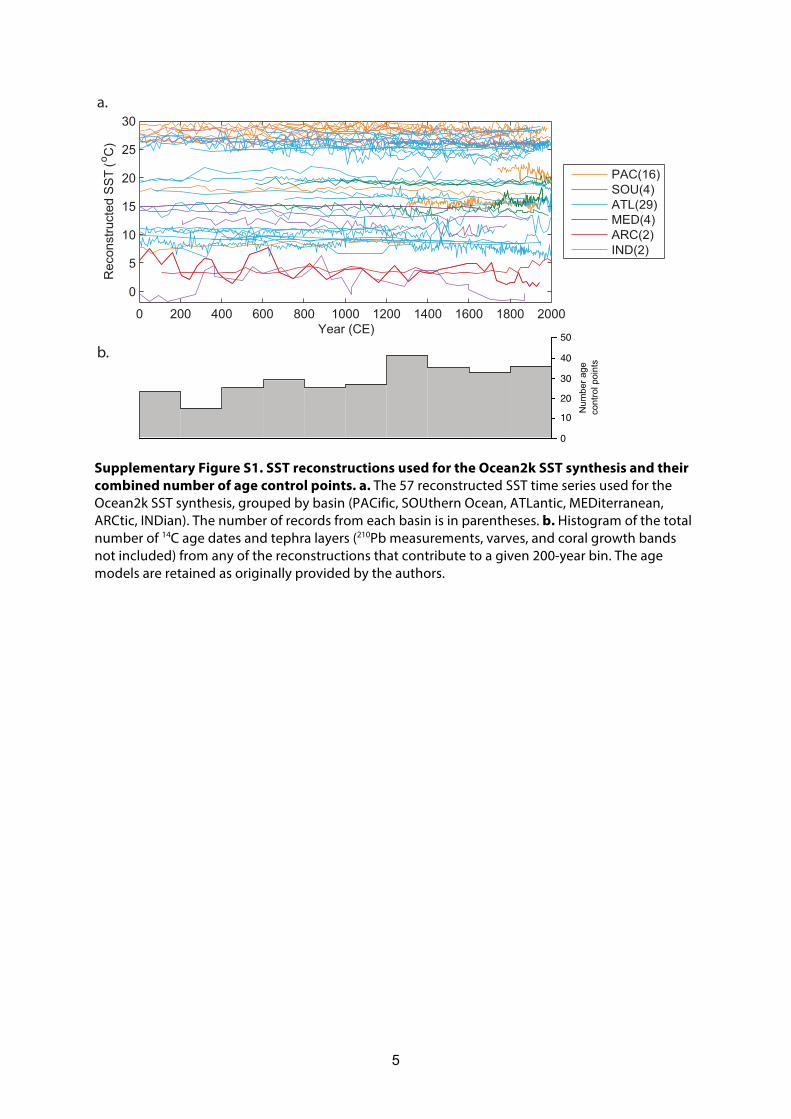
Supplementary Figure S1. SST reconstructions used for the Ocean2k SST synthesis and their combined number of age control points. a. The 57 reconstructed SST time series used for the Ocean2k SST synthesis, grouped by basin (PACific, SOUthern Ocean, ATLantic, MEDiterranean, ARCtic, INDian). The number of records from each basin is in parentheses. b. Histogram of the total number of 14C age dates and tephra layers (210Pb measurements, varves, and coral growth bands not included) from any of the reconstructions that contribute to a given 200-year bin. The age models are retained as originally provided by the authors.

0 200 400 600 800 1000 1200 1400 1600 1800 2000

0

5

10

15

20

25

30

Year (CE)

Rec

onst

ruct

ed S

ST (o C

)

Num

ber a

geco

ntro

l poi

nts

0

10203040

50

a.

b.

PAC(16)SOU(4)ATL(29)MED(4)ARC(2)IND(2)

6

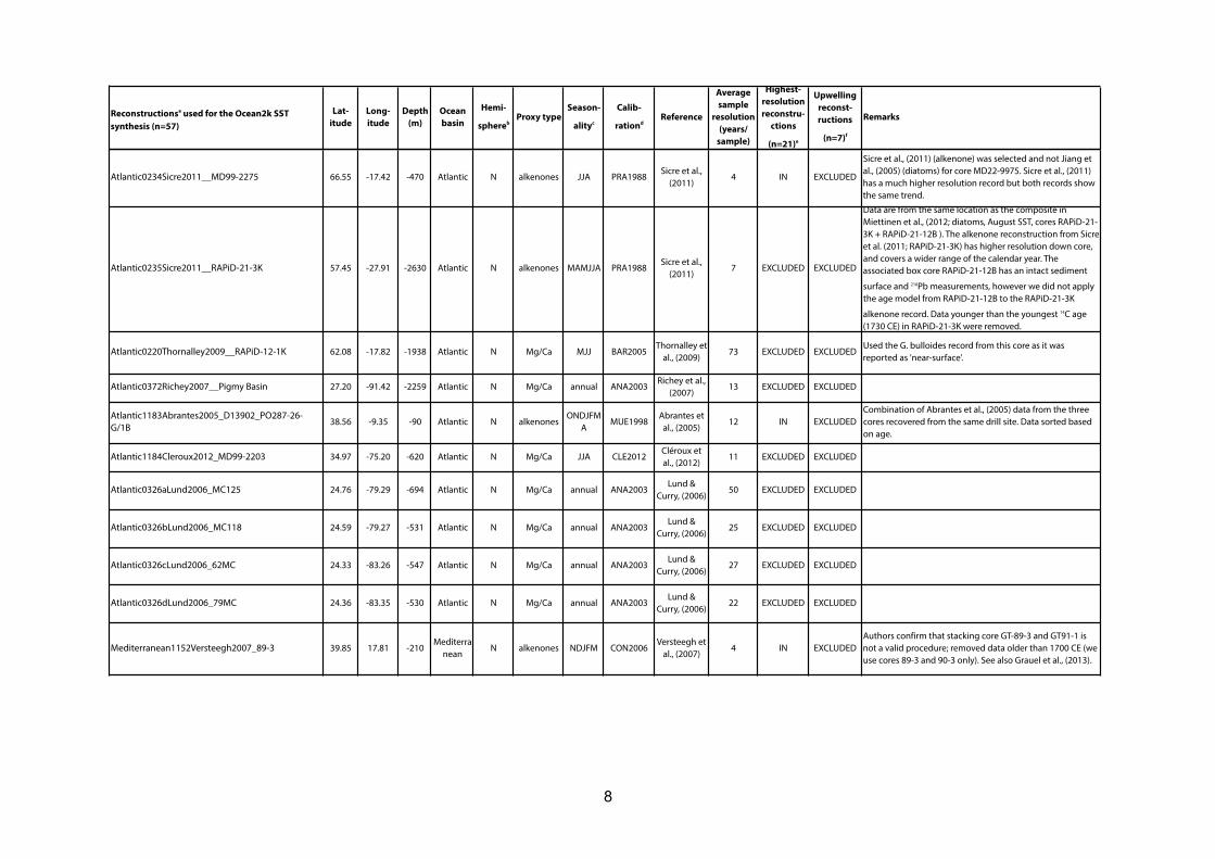
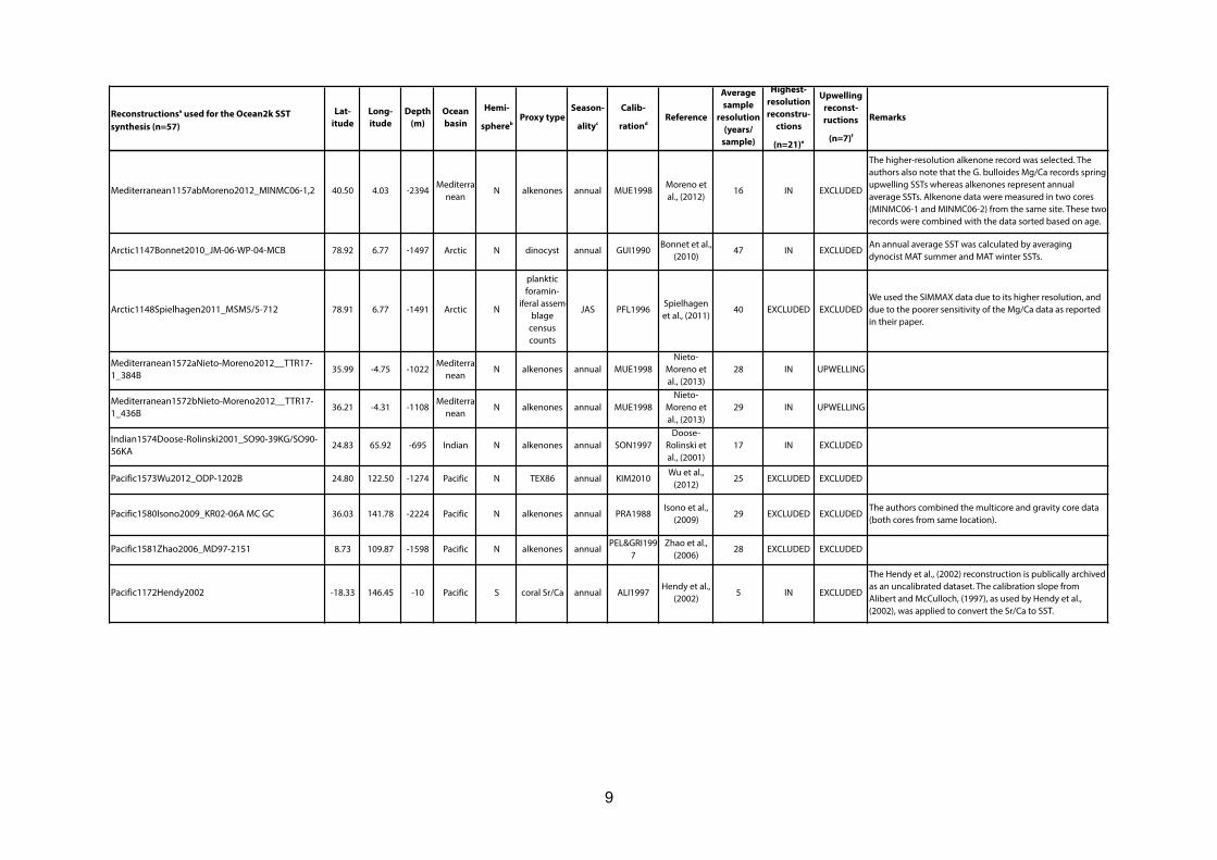
Supplementary Table S1. Metadata for the 57 reconstructions used in the Ocean2k SST synthesis.

Supplementary Table S1. Metadata for the 57 reconstructions used in the Ocean2k SST synthesis.

Reconstructionsa used for the Ocean2k SST synthesis (n=57)

Lat-itude

Long-itude

Depth (m)

Ocean basin

Hemi-

spherebProxy type

Season-

alityc

Calib-

rationdReference

Average sample

resolution (years/

sample)

Highest-resolution reconstru-

ctions

(n=21)e

Upwelling reconst-ructions

(n=7)f

Remarks

Pacific0335aOppo2009_MC31,BJ8-03-32GGC,BJ8-03-34GGC -3.53 119.20 -472 Pacific S Mg/Ca annual ANA2003

Oppo et al., (2009)

11 IN EXCLUDEDCombination of Oppo et al., (2009) data from the three cores recovered from the same drill site. Data sorted based on age.

Pacific0291Newton2011_MD98-2160 -5.20 117.48 -1185 Pacific S Mg/Ca annual DEK2002Newton et al., (2011)

11 EXCLUDED EXCLUDEDData archived as Mg/Ca values only. Data converted to SST using the calibration of Dekens et al., 2002, as per the original publication.

Pacific0173aLinsley2010_13GGC -7.40 115.20 -594 Pacific S Mg/Ca annual ANA2003Linsley et al.,

(2010)34 EXCLUDED EXCLUDED

Pacific0185Stott2007_MD98-2181 6.30 125.83 -2114 Pacific N Mg/Ca annual ANA2003Stott et al.,


WDC-paleoclimatology Data Contribution Series # 2007-092 Readme for Stott et al., (2007) notes calibration with Anand et al., (2003).

Pacific0118Stott2007_MD98-2176 -5.00 133.44 -2382 Pacific S Mg/Ca annual ANA2003Stott et al.,


WDC-paleoclimatology Data Contribution Series # 2007-092 Readme for Stott et al., (2007) notes calibration with Anand et al., (2003).

Pacific1177Pahnke2007_MC33 4.67 -77.96 -2200 Pacific N alkenones annual PRA1988Pahnke et al.,

(2007)12 IN EXCLUDED

Pacific1178Pahnke2007_MC14 4.85 -77.61 -884 Pacific N alkenones annual PRA1988Pahnke et al.,

(2007)9 IN EXCLUDED

Pacific0328aHarada2004_MR00-K03-PC01 46.32 152.53 -2793 Pacific N alkenones JA PRA1988 Harada et al., (2004)

58 EXCLUDED EXCLUDED

Southern0045aLamy2002_GeoB3313-1 -41.00 -74.45 -852 Southern S alkenones annual PRA1988Lamy et al.,


Southern0485aMohtadi2007_GeoB7186-3 -44.15 -75.16 -1169 Southern S alkenones annual PRA1988Mohtadi et al., (2007)


Southern1159aSepulveda2009_CF7-PC33 -44.33 -72.97 -510 Southern S alkenones SON PRA1988Sepúlveda et

al., (2009)25 EXCLUDED EXCLUDED

Southern0483aShevenell2011_ODP-1098B -64.87 -64.20 -1011 Southern S TEX86 SO KIM2008Shevenell et


We used the publically archived data from PANGAEA, dated 2011.

Atlantic1565Calvo2002_ MD95-2011 66.97 7.63 -1048 Atlantic N alkenones JJAPRA&WAK1

987Calvo et al.,


The Calvo et al., (2002) data set was selected instead of Dolven et al., (2002) because it had higher resolution. Berner et al., (2011) provides additional dates, though with age reversals, so we retain the age model of Calvo et al., (2002).

Atlantic0195dSachs2007__GGC-30 43.53 -62.48 -250 Atlantic N alkenones annual PRA1988Sachs et al.,


Atlantic0195aKeigwin2005__OCE326 26GGC 43.48 -54.87 -3975 Atlantic N alkenones annualPRA&WAK1

987Keigwin et al., (2005)


7


Lat-itude

Long-itude

Depth (m)

Ocean basin

Hemi-

spherebProxy type

Season-

alityc

Calib-

rationdReference

Average sample

resolution (years/

sample)


ctions

(n=21)e


(n=7)f

Remarks

Atlantic0368Keigwin2003__MC-29D 45.89 -62.80 -250 Atlantic N alkenones annual PRA1988Keigwin et al., (2003)


Atlantic1578Kim2007_GeoB6007-2 30.85 -10.27 -900 Atlantic N alkenones annual MUE1998Kim et al.,


Revised age model for GeoB6007-2 from Morley et al., (2011) was applied to GeoB6007-2 alkenone data from Kim et al., (2007).

Atlantic0255aSaenger2011__CH07-98-MC22 32.78 -76.28 -1895 Atlantic N Mg/Ca annual ANA2003Saenger et al., (2011)


Atlantic0255bSaenger2011__KNR140_2_59GGC 32.98 -76.32 -1205 Atlantic N Mg/Ca annual ANA2003Saenger et al., (2011)


Atlantic0487McGregor2007__GeoB6008-1, GeoB6008-2

30.85 -10.10 -355 Atlantic N alkenones annual PRA1988McGregor et

al., (2007)11 IN UPWELLING

Atlantic0043aRichey2009__Garrison_PE07-2 26.68 -93.93 -1570 Atlantic N Mg/Ca annual BLA2007Richey et al.,


Note that raw 14C ages in Richey et al. (2009) are reported with the 400-year reservoir age subtracted (Pers. Comm. J. Richey 1 April 2015).

Atlantic0043bRichey2009__Fisk_PE07-5I 27.55 -93.93 -817 Atlantic N Mg/Ca annual BLA2007Richey et al.,


Atlantic0039Black2007__PL07-73 BC 10.77 -64.77 -450 Atlantic N Mg/Ca MAM ANA2003Black et al.,

(2007)4 IN EXCLUDED

Atlantic0040Lea2003__PL07-39PC 10.70 -64.94 -790 Atlantic N Mg/Ca annual DEK2002Lea et al.,


Atlantic0403deMenocal2000__ODP-108-658C 20.75 -18.58 -2263 Atlantic N

planktic foramin-iferal ass-emblage census counts

annualRUD&GLO1

975deMenocal et al., (2000)


August and February SST data averaged to give an annual mean SST. The deMenocal et al., (2000) data set was selected instead of Zhao et al., (1995) because it had higher resolution. Trends between the two cores were similar.

Atlantic0488Kuhnert2011__ GeoB9501-5 16.84 -16.73 -323 Atlantic N Mg/Ca JASOND ANA2003Kuhnert &

Mulitza, (2011)

11 IN EXCLUDEDCombination of data from GeoB 9501–4 and GeoB 9501–5. Data combined based on age sort order.

Atlantic0316Weldeab2007__MD03-2707 2.50 9.38 -1295 Atlantic N Mg/Ca annual ANA2003Weldeab et al., (2007)


Atlantic0484Leduc2010_GeoB8331-4+GeoB8331-2 -29.14 16.72 -97 Atlantic S alkenones annual MUE1998Leduc et al.,

(2010)16 IN UPWELLING

Atlantic0219Came2007__ODP-162-984 61.43 -24.08 -1648 Atlantic N Mg/Ca annual vLA2005Came et al.,


Atlantic0058Richter2009__ENAM9606,M200309 55.50 -13.90 -84 Atlantic N Mg/Ca AMJJ ANA2003Richter et al.,


8


Lat-itude

Long-itude

Depth (m)

Ocean basin

Hemi-

spherebProxy type

Season-

alityc

Calib-

rationdReference

Average sample

resolution (years/

sample)


ctions

(n=21)e


(n=7)f

Remarks

Atlantic0234Sicre2011__MD99-2275 66.55 -17.42 -470 Atlantic N alkenones JJA PRA1988Sicre et al.,

(2011)4 IN EXCLUDED

Sicre et al., (2011) (alkenone) was selected and not Jiang et al., (2005) (diatoms) for core MD22-9975. Sicre et al., (2011) has a much higher resolution record but both records show the same trend.

Atlantic0235Sicre2011__RAPiD-21-3K 57.45 -27.91 -2630 Atlantic N alkenones MAMJJA PRA1988Sicre et al.,


Data are from the same location as the composite in Miettinen et al., (2012; diatoms, August SST, cores RAPiD-21-3K + RAPiD-21-12B ). The alkenone reconstruction from Sicre et al. (2011; RAPiD-21-3K) has higher resolution down core, and covers a wider range of the calendar year. The associated box core RAPiD-21-12B has an intact sediment

surface and 210Pb measurements, however we did not apply the age model from RAPiD-21-12B to the RAPiD-21-3K

alkenone record. Data younger than the youngest 14C age (1730 CE) in RAPiD-21-3K were removed.

Atlantic0220Thornalley2009__RAPiD-12-1K 62.08 -17.82 -1938 Atlantic N Mg/Ca MJJ BAR2005Thornalley et


Used the G. bulloides record from this core as it was reported as 'near-surface'.

Atlantic0372Richey2007__Pigmy Basin 27.20 -91.42 -2259 Atlantic N Mg/Ca annual ANA2003Richey et al.,


Atlantic1183Abrantes2005_D13902_PO287-26-G/1B 38.56 -9.35 -90 Atlantic N alkenones

ONDJFMA

MUE1998Abrantes et

al., (2005)12 IN EXCLUDED

Combination of Abrantes et al., (2005) data from the three cores recovered from the same drill site. Data sorted based on age.

Atlantic1184Cleroux2012_MD99-2203 34.97 -75.20 -620 Atlantic N Mg/Ca JJA CLE2012Cléroux et al., (2012)


Atlantic0326aLund2006_MC125 24.76 -79.29 -694 Atlantic N Mg/Ca annual ANA2003Lund &

Curry, (2006)50 EXCLUDED EXCLUDED

Atlantic0326bLund2006_MC118 24.59 -79.27 -531 Atlantic N Mg/Ca annual ANA2003Lund &


Atlantic0326cLund2006_62MC 24.33 -83.26 -547 Atlantic N Mg/Ca annual ANA2003Lund &


Atlantic0326dLund2006_79MC 24.36 -83.35 -530 Atlantic N Mg/Ca annual ANA2003Lund &


Mediterranean1152Versteegh2007_89-3 39.85 17.81 -210Mediterra

neanN alkenones NDJFM CON2006

Versteegh et al., (2007)

4 IN EXCLUDEDAuthors confirm that stacking core GT-89-3 and GT91-1 is not a valid procedure; removed data older than 1700 CE (we use cores 89-3 and 90-3 only). See also Grauel et al., (2013).

9


Lat-itude

Long-itude

Depth (m)

Ocean basin

Hemi-

spherebProxy type

Season-

alityc

Calib-

rationdReference

Average sample

resolution (years/

sample)


ctions

(n=21)e


(n=7)f

Remarks

Mediterranean1157abMoreno2012_MINMC06-1,2 40.50 4.03 -2394Mediterra

neanN alkenones annual MUE1998

Moreno et al., (2012)

16 IN EXCLUDED

The higher-resolution alkenone record was selected. The authors also note that the G. bulloides Mg/Ca records spring upwelling SSTs whereas alkenones represent annual average SSTs. Alkenone data were measured in two cores (MINMC06-1 and MINMC06-2) from the same site. These two records were combined with the data sorted based on age.

Arctic1147Bonnet2010_JM-06-WP-04-MCB 78.92 6.77 -1497 Arctic N dinocyst annual GUI1990Bonnet et al.,


An annual average SST was calculated by averaging dynocist MAT summer and MAT winter SSTs.

Arctic1148Spielhagen2011_MSM5/5-712 78.91 6.77 -1491 Arctic N

planktic foramin-

iferal assem-blage

census counts

JAS PFL1996Spielhagen et al., (2011)

40 EXCLUDED EXCLUDEDWe used the SIMMAX data due to its higher resolution, and due to the poorer sensitivity of the Mg/Ca data as reported in their paper.

Mediterranean1572aNieto-Moreno2012__TTR17-1_384B

35.99 -4.75 -1022Mediterra


Nieto-Moreno et al., (2013)

28 IN UPWELLING

Mediterranean1572bNieto-Moreno2012__TTR17-1_436B

36.21 -4.31 -1108Mediterra



29 IN UPWELLING

Indian1574Doose-Rolinski2001_SO90-39KG/SO90-56KA

24.83 65.92 -695 Indian N alkenones annual SON1997Doose-

Rolinski et al., (2001)

17 IN EXCLUDED

Pacific1573Wu2012_ODP-1202B 24.80 122.50 -1274 Pacific N TEX86 annual KIM2010Wu et al.,


Pacific1580Isono2009_KR02-06A MC GC 36.03 141.78 -2224 Pacific N alkenones annual PRA1988Isono et al.,


The authors combined the multicore and gravity core data (both cores from same location).

Pacific1581Zhao2006_MD97-2151 8.73 109.87 -1598 Pacific N alkenones annualPEL&GRI199

7Zhao et al.,


Pacific1172Hendy2002 -18.33 146.45 -10 Pacific S coral Sr/Ca annual ALI1997Hendy et al.,

(2002)5 IN EXCLUDED

The Hendy et al., (2002) reconstruction is publically archived as an uncalibrated dataset. The calibration slope from Alibert and McCulloch, (1997), as used by Hendy et al., (2002), was applied to convert the Sr/Ca to SST.

10


Lat-itude

Long-itude

Depth (m)

Ocean basin

Hemi-

spherebProxy type

Season-

alityc

Calib-

rationdReference

Average sample

resolution (years/

sample)


ctions

(n=21)e


(n=7)f

Remarks

Pacific1582Zhao2000_Hendy2012_Schimmelmann2013_SABA87-2, SABA88-1

34.23 -120.02 -590 Pacific N alkenones annual PRA1988

Zhao et al., (2000);

Hendy et al., (2012);

Schimmel-mann et al.,

(2013)

1 IN EXCLUDED

Zhao et al., (2000) alkenone record with the age model from Hendy et al., (2012) and Schimmelmann et al., (2013). Combination of two cores (SABA87-2 and SABA88-1) recovered from the same drill site. Data sorted based on age.

Pacific1571Gutierrez2011_B0406 -14.13 -76.50 -299 Pacific S alkenones annualPRA&WAK1

987Gutierrez et

al., (2011)3 IN UPWELLING

Pacific1575Goni2006_BC-43 27.90 -111.66 -655 Pacific N alkenones annual PRA1988Goñi et al.,


Atlantic1576Goni2006_MC-4 10.65 -64.66 -432 Atlantic N alkenones annual PRA1988Goñi et al.,


Pacific1577Newton2011_MD98-2177 1.40 119.08 -968 Pacific N Mg/Ca annual DEK2002Newton et al., (2011)

17 EXCLUDED EXCLUDEDData archived as Mg/Ca values only. Data converted to SST using the calibration of Dekens et al., (2002), as per the original publication.

Indian1579Saraswat2013_SK237-GC04 10.98 75.00 -1245 Indian N Mg/Ca annual DEK2002Saraswat et al., (2013)


[Ocean basin][Ocean2k metadatabase number][Publication first author and year]_[core number(s)]_[optional additional metadata].b N: Northern hemisphere; S: Southern hemisphere

d Calibrations used by reconstruction authorsMUE1998: T(sediments) = (Uk’37-0.044)/0.033, [Müller et al., 1998; global (60S-60N), 0-29ºC, annual at 0 m, n=370, R2=0.958]CON2006: T(sediments) = 29.876*( Uk’37)-1.334, (Conte et al., (2006); sediments, global, annual at 0 m, -1-29ºC, n=592, R2=0.97, error ±1.1°C)PRA1988: T(cultures) = (Uk'37-0.039)/(0.034), [Prahl et al., 1988; cultures E. huxleyi, 8-25ºC, n=22; R2=0.994]PRA&WAK1987: T(cultures) = (UK37+0.11)/0.04, [Prahl & Wakeham, 1987; cultures E. huxleyi, 8-25ºC, n=5; R2=0.989]SON1997: T(sediments) = (Uk'37-0.316)/(0.023), [Sonzogni et al., 1997; sediments, Indian Ocean, 24-29ºC, production at 0-10 m, n=54, R2=0.856]PEL&GRI1997: T(sediments)= (Uk'37-0.092)/(0.031), [Pelejero & Grimalt, 1997; sediments, South China Sea, 24-29ºC, annual at 0-30 m, n=31, R2=0.858]DEK2002: Mg/Ca=0.38*exp(0.09*[SST-0.61 (core depth km)]), [Dekens et al., 2002; core tops; G ruber]ANA2003: Mg/Ca=0.38*exp(0.09*SST), multiple species; Mg/Ca =0.449*exp(0.09*SST), G. ruber, [Anand et al., 2003; sediment trap; error ±1.2°C]BLA2007: Mg/Ca=0.048*exp(0.173*SST), [Black et al., 2007; G. bulloides]vLA2005: Mg/Ca=0.51*exp(0.10*T), [von Langen et al., 2005; N. pachyderma]BAR2005: Mg/Ca=0.794*exp(0.10*SST), [Barker et al., 2005, in combination with Thornalley et al., 2009; error ±1.3°C]CLE2012: T=(1/0.07)ln((Mg/Ca)/0.76), (Cléroux et al., (2012); error ±1.3°C)KIM2008: SST (°C)= (0.0125*TEX86)+0.3038, [Kim et al., 2008, error ±2.2°C]KIM2010: SST=(68.4*TEX86H)+38.6, [Kim et al., 2010]PFL1996: SIMMAX, Modern Analogue Technique, [Pflaumann et al., 1996]GUI1990: MAT, Modern Analogue Technique, [Guiot, 1990]RUD&GLO1975: F13' Transfer Function, [Ruddiman & Glover, 1975; error ±1.6°C]ALI1997: Sr/Ca SST sensitivity = -0.0615 mmol/mol/°C, [Alibert and McCulloch 1997]e Highest resolution reconstructions used in Supplement Figure S7. See Supplementary Discussion on 20th century Ocean2k synthesis for selection criteria.f Upwelling reconstructions used in Figure 2 and Supplement Figure S7. See Supplementary Methods and Supplementary Table S3 for selection criteria.

a Reconstruction is the reconstruction name used by the PAGES Ocean2k Group when compiling the data. The reconstruction name is compiled as follows:

c Annual is the calendar year. Any reconstruction with a documented seasonal bias is specificed by month (JFMAMJJASON or D).

11

Supplementary Table S2. URLs for the 57 Ocean2k reconstruction data products.


Reference URL for data product

Pacific0335aOppo2009_MC31,BJ8-03-32GGC,BJ8-03-34GGC

Oppo et al., (2009)

http://www.ncdc.noaa.gov/paleo/pubs/oppo2009/oppo2009.html

Pacific0291Newton2011_MD98-2160

Newton et al., (2011)

http://hurricane.ncdc.noaa.gov/pls/paleox/f?p=519:1:8614211809409317::::P1_STUDY_ID:12906 and/or http://hurricane.ncdc.noaa.gov/pls/paleox/f?p=519:1:1696330230021088::::P1_STUDY_ID:5534

Pacific0173aLinsley2010_13GGC Linsley et al., (2010)

ftp://ftp.ncdc.noaa.gov/pub/data/paleo/contributions_by_author/linsley2010/linsley2010.txt

Pacific0185Stott2007_MD98-2181 Stott et al., (2007)

http://hurricane.ncdc.noaa.gov/pls/paleox/f?p=519:1:3757743008453739::::P1_STUDY_ID:6400

Pacific0118Stott2007_MD98-2176 Stott et al., (2007)


Pacific1177Pahnke2007_MC33 Pahnke et al., (2007)


Pacific1178Pahnke2007_MC14 Pahnke et al., (2007)


Pacific0328aHarada2004_MR00-K03-PC01

Harada et al., (2004)

ftp://ftp.ncdc.noaa.gov/pub/data/paleo/contributions_by_author/harada2004/harada2004.txt

Southern0045aLamy2002_GeoB3313-1

Lamy et al., (2002)

ftp://ftp.ncdc.noaa.gov/pub/data/paleo/contributions_by_author/lamy2002/

Southern0485aMohtadi2007_GeoB7186-3

Mohtadi et al., (2007)

http://doi.pangaea.de/10.1594/PANGAEA.676709

Southern1159aSepulveda2009_CF7-PC33

Sepúlveda et al., (2009)


Southern0483aShevenell2011_ODP-1098B

Shevenell et al., (2011)

http://doi.pangaea.de/10.1594/PANGAEA.769699 and/or ftp://ftp.ncdc.noaa.gov/pub/data/paleo/contributions_by_author/shevenell2007

Atlantic1565Calvo2002_ MD95-2011

Calvo et al., (2002)


Atlantic0195dSachs2007__GGC-30

Sachs et al., (2007)

ftp://ftp.ncdc.noaa.gov/pub/data/paleo/contributions_by_author/sachs2007

Atlantic0195aKeigwin2005__OCE326 26GGC

Keigwin et al., (2005)

ftp://ftp.ncdc.noaa.gov/pub/data/paleo/contributions_by_author/keigwin2005 and/or ftp://ftp.ncdc.noaa.gov/pub/data/paleo/contributions_by_author/sachs2007

Atlantic0368Keigwin2003__MC-29D

Keigwin et al., (2003)

ftp://ftp.ncdc.noaa.gov/pub/data/paleo/contributions_by_author/keigwin2003/keigwin2003.txt

Atlantic1578Kim2007_GeoB6007-2

Kim et al., (2007)


Atlantic0255aSaenger2011__CH07-98-MC22

Saenger et al., (2011)


Atlantic0255bSaenger2011__KNR140_2_59GGC

Saenger et al., (2011)


Atlantic0487McGregor2007__GeoB6008-1, GeoB6008-2

McGregor et al., (2007)


Atlantic0043aRichey2009__Garrison_PE07-2

Richey et al., (2009)


Atlantic0043bRichey2009__Fisk_PE07-5I



Atlantic0039Black2007__PL07-73 BC

Black et al., (2007)


Atlantic0040Lea2003__PL07-39PC Lea et al., (2003)


Atlantic0403deMenocal2000__ODP-108-658C

deMenocal et al., (2000)


Atlantic0488Kuhnert2011__ GeoB9501-5

Kuhnert & Mulitza, (2011)

http://doi.pangaea.de/10.1594/PANGAEA.773754 and/or http://doi.pangaea.de/10.1594/PANGAEA.773758

Atlantic0316Weldeab2007__MD03-2707

Weldeab et al., (2007)


Atlantic0484Leduc2010_GeoB8331-4+GeoB8331-2

Leduc et al., (2010)


Atlantic0219Came2007__ODP-162-984

Came et al., (2007)

ftp://ftp.ncdc.noaa.gov/pub/data/paleo/contributions_by_author/came2007/came2007.txt

Atlantic0058Richter2009__ENAM9606,M200309

Richter et al., (2009)

ftp://ftp.ncdc.noaa.gov/pub/data/paleo/contributions_by_author/richter2009/richter2009.txt

Atlantic0234Sicre2011__MD99-2275

Sicre et al., (2011)

http://hurricane.ncdc.noaa.gov/pls/paleox/f?p=519:1:::::P1_STUDY_ID:12359

12


Reference URL for data product

Atlantic0235Sicre2011__RAPiD-21-3K

Sicre et al., (2011)

http://hurricane.ncdc.noaa.gov/pls/paleox/f?p=519:1:::::P1_STUDY_ID:12359

Atlantic0220Thornalley2009__RAPiD-12-1K

Thornalley et al., (2009)

ftp://ftp.ncdc.noaa.gov/pub/data/paleo/contributions_by_author/thornalley2009/thornalley2009.txt

Atlantic0372Richey2007__Pigmy Basin



Atlantic1183Abrantes2005_D13902_PO287-26-G/1B

Abrantes et al., (2005)


Atlantic1184Cleroux2012_MD99-2203

Cléroux et al., (2012)


Atlantic0326aLund2006_MC125 Lund & Curry, (2006)

ftp://ftp.ncdc.noaa.gov/pub/data/paleo/contributions_by_author/lund2006/lund2006.txt

Atlantic0326bLund2006_MC118 Lund & Curry, (2006)


Atlantic0326cLund2006_62MC Lund & Curry, (2006)


Atlantic0326dLund2006_79MC Lund & Curry, (2006)


Mediterranean1152Versteegh2007_89-3

Versteegh et al., (2007)


Mediterranean1157abMoreno2012_MINMC06-1,2

Moreno et al., (2012)


Arctic1147Bonnet2010_JM-06-WP-04-MCB

Bonnet et al., (2010)


Arctic1148Spielhagen2011_MSM5/5-712

Spielhagen et al., (2011)


Mediterranean1572aNieto-Moreno2012__TTR17-1_384B



Mediterranean1572bNieto-Moreno2012__TTR17-1_436B



Indian1574Doose-Rolinski2001_SO90-39KG/SO90-56KA

Doose-Rolinski et al., (2001)


Pacific1573Wu2012_ODP-1202B Wu et al., (2012)

http://doi.pangaea.de/10.1594/PANGAEA.803648?format=html

Pacific1580Isono2009_KR02-06A MC GC

Isono et al., (2009)


Pacific1581Zhao2006_MD97-2151 (Zhao) et al., 2006


Pacific1172Hendy2002 Hendy et al., (2002)

ftp://ftp.ncdc.noaa.gov/pub/data/paleo/coral/west_pacific/great_barrier/hendydata.txt

Pacific1582Zhao2000_Hendy2012_Schimmelmann2013_SABA87-2, SABA88-1

Zhao et al., (2000); Hendy et al., (2012); Schimmel-mann et al., (2013)

http://www.ncdc.noaa.gov/paleo/study/17755

Pacific1571Gutierrez2011_B0406 Gutierrez et al., (2011)

http://doi.pangaea.de/10.1594/PANGAEA.808961?format=html

Pacific1575Goni2006_BC-43 Goñi et al., (2006)


Atlantic1576Goni2006_MC-4 Goñi et al., (2006)


Pacific1577Newton2011_MD98-2177

Newton et al., (2011)


Indian1579Saraswat2013_SK237-GC04

Saraswat et al., (2013)

ftp://ftp.ncdc.noaa.gov/pub/data/paleo/contributions_by_author/saraswat2013/saraswat2013-sk237gc04.txt

13

SST reconstructions and calibrations

Datasets reporting thermocline temperatures were omitted. It was assumed that the SST calibrations reported in the original publication were the most appropriate for the dataset. If only native data were archived in data repositories, they were converted to SST with the calibration used in the original publication. SST errors are estimated at 1.66ºC (1.28ºC, 2.05ºC (5th, 95th percentiles)); see Supplementary Section 4 for calculation; Supplementary Fig. S6). The standardized reconstructions likely mitigate biases introduced by use of different calibrations.

Age model criteria

The reconstructions were required to have at least two age dates between 200 BCE (before Common Era) and present. If a record had an age whose 2σ error overlapped with 200 BCE it was deemed to pass the age model criteria. Age dating was primarily based on radiocarbon dating, 210Pb dating (with or without 137Cs), varved sediment or coral growth band counting, cross-correlation of dated tephra layers, and/or complemented by a δ13C record of the Suess Effect. Core-top ages based on the presence of the sediment-water interface were included, and in these cases the core-top age was taken as the year the core was collected. Reconstructions were excluded if they included large age reversals, or if the age dating was based on benthic organisms, since the radiocarbon reservoir age of subsurface waters may have varied greatly in space and time. All age models were converted to the CE/BCE time scale. Age model data reported as ‘Modern’ or 0 years before present were checked in the original publication to ascertain the CE/BCE time scale equivalent.

Beyond conversion to the CE/BCE time scale, no modification or reinterpretation of the published age model was performed. A comparison between published age models and a recalculation of age models using Bayesian techniques for a subset of randomly selected reconstructions did not yield significant differences at 200-year compositing resolution (not shown). Further, changes to the radiocarbon marine calibration curve for the 0-1950 CE interval are trivial and are unlikely to affect our results (Supplementary Fig. S7; Bard et al., 1993; Stuiver and Braziunas, 1993; Stuiver et al., 1998; Hughen et al., 2004; Reimer et al., 2009; Reimer et al., 2013). Together, these findings suggest that revision of the age models would not yield more accurate results. Therefore, we retain the published age models for our synthesis. By retaining the original age models we also retain the expert original-author judgment that developed those age models. Age model queries are noted in Supplementary Table S1.

Finally, only data between bracketing ages were included i.e. data younger than the youngest date were removed and data older than the oldest date were removed. The number of dates per bin for the 57 reconstructions is given in Supplementary Figure S1b.

14

Supplementary Figure S2. Radiocarbon marine calibration curves (Bard et al., 1993; Stuiver and Braziunas, 1993; Stuiver et al., 1998; Hughen et al., 2004; Reimer et al., 2009; Reimer et al., 2013) used by various reconstructions contributing to the Ocean2k SST synthesis. For the 0–1950 CE interval the curves show minimal differences. As a consequence we have not recalibrated age models.

Special cases – multiple SST estimates

Where multiple types of SST estimates were measured in the same sediment core (published by either the same or different authors; Supplementary Fig. S3), the reconstruction with the highest measurement resolution was selected rather than taking the two different reconstructions as two independent datasets, to minimize signal aliasing, and to avoid over-sampling particular locations and exacerbating regional biases. If the reconstructions have similar resolution, we followed the authors’ published recommendation for the most reliable SST estimate or we use the estimate most likely to represent mean annual SST.

There were six instances of multiple SST reconstructions from the same site (also noted in Supplementary Table S1). In all instances one reconstruction was clearly at a higher resolution than the other; this highest-resolution reconstruction was used in our calculations.

In general, comparison of multiple SST estimates from the same sediment core (Supplementary Fig. S3) shows agreement for the trend, but differences in absolute temperature and in some cases variance. See Supplementary Section 6 for a full discussion of calibration, seasonality, and other proxy-specific possible sources of these differences. Specific additional factors worth noting with regard to selection of one reconstruction over another are: for core MSM5/5-712 the lower-resolution Mg/Ca reconstruction was interpreted

15

as having increased variability relative to the SIMMAX foraminifera assemblage SST reconstruction, since the SSTs were approximately 3°C below the reliability limit for the foraminiferal Mg/Ca method (Spielhagen et al., 2011); for core MINMC06-1,2 the alkenone SST reconstruction had the highest resolution and was most likely to reflect mean annual SST, whereas the Mg/Ca SST reconstruction instead reflected spring upwelling (Moreno et al., 2012); for core RAPiD-21-3K the higher-resolution alkenone SST reconstruction (Sicre et al., 2011) is reported to reflect more of the calendar year (MAMJJA) than the lower resolution diatom-based August SST reconstruction (Miettinen et al., 2012). Despite differences in same-site SST reconstructions, the binned and standardized results are similar (Supplementary Fig. S3).

Datasets were combined when records of the same proxy type originated from cores collected from the same site. In this situation there is no a priori reason to assume that one record is better than the other and the differences between the records provide a measure of external reproducibility. The reconstructions were merged and sorted in the depth/age domain.

16

Supplementary Figure S3. Multiple SST reconstructions from the same core. a. SST datasets used in the Ocean2k SST synthesis (solid lines) and the additional SST reconstruction available from the same core (dashed line). b. As for a) except reconstructions have been averaged into 200-year bins and standardized. Reconstructions are for cores: MSM5/5-712 (yellow and brown; Spielhagen et al., 2011); MINMC06-1,2 (pink and red; Moreno et al., 2012); ODP-108-658C (green and dark green; deMenocal et al., 2000; Zhao et al., 1995); RAPiD-21-3K (orange and dark orange; (Sicre et al., 2011; Miettinen et al., 2012); MD99-2275 (grey and black; Sicre et al., 2011; Jiang et al., 2005); MD95-2011 (light blue and dark blue; Calvo et al., 2002; Dolven et al., 2002). Reconstruction types are given in the legend. The highest-resolution reconstruction was selected from each core, or if of similar resolution, the reconstruction more representative of annual averages or the greater span for the 1-2000 CE interval was selected. Paired reconstructions from the same core show similar standardized trends.

Reconstructions from upwelling regions

A record was included as an upwelling record if the original publication provides evidence that the site is from an upwelling region and offers evidence that their proxy SSTs represent the upwelling season, or if the proxy represents mean annual SST, when the mean annual SST is influenced by upwelling intensity. Justification for each reconstruction designated as from an upwelling region is given in Supplementary Table S3.

100 300 500 700 900 1100 1300 1500 1700 1900Year (CE)

11

12

132468

10 8

10

12

1418

19

20

21

22

15

18

21

2

4

6

8Se

a Su

rface

Tem

pera

ture

(o C)

100 300 500 700 900 1100 1300 1500 1700 1900Year (CE)

-2-1012

-2-1012

-2-1012

-2-1012

-2-1012

-2-1012

Foram (SIMMAX)Foram (Mg/Ca)Alkenone(Uk'

37)Foram (Mg/Ca)

Alkenone(Uk'37)

Diatom (Trans. funct.)Alkenone(Uk'

37)Radiolaria(Trans. funct.)

Foram (Trans. funct.)Alkenone(Uk'

37)Alkenone(Uk'

37)Diatom (Trans. funct.)

Stan

dard

ized

ano

mal

y (s

.d. u

nits

)

MD95-2011

MD99-2275

RAPiD21-3K

ODP108-658C

MINMC06-1,2

MSM5/5-712

a b

17

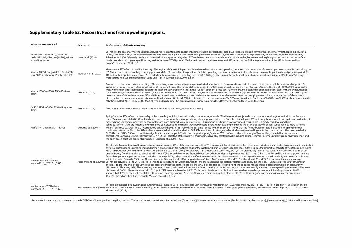
Supplementary Table S3. Reconstructions from upwelling regions.

Reconstruction name a Reference Evidence for / relation to upwelling

Atlantic0484Leduc2010_GeoB8331-4+GeoB8331-2_alkenone(Muller)_winter (upwelling) season

Leduc et al. (2010)

SST re!ects the seasonality of the Benguela upwelling: "In an attempt to improve the understanding of alkenone‐based SST reconstructions in terms of seasonality as hypothesized in Leduc et al. (2010), Schneider et al. (2010) have used satellite data for mapping the existing relationship between the annual cycles of SST and of primary productivity. The seasonality index developed by Schneider et al. (2010) broadly predicts an increased primary productivity when SST are below the mean ‐ annual value at mid‐latitudes, because upwelling bringing nutrients to the sea surface synchronously act to trigger algal blooming and to decrease SST (Figure 1c). We hence interpret the alkenone derived SST records of the BUS as representative of the SST during upwelling events.” Leduc et al. (2010), p.2

Atlantic0487McGregor2007__GeoB6008-1, GeoB6008-2_ alkenone(Prahl et al., 1988) Mc Gregor et al. (2007)

Mean annual SST re!ects upwelling intensity: “The region o# Cape Ghir is particularly well suited for the study of upwelling because it constitutes one of the most persistent upwelling cells along the NW African coast, with upwelling occurring year-round (8–10). Sea surface temperatures (SSTs) in upwelling zones are sensitive indicators of changes in upwelling intensity and prevailing winds (8, 11), and, in the Cape Ghir area, cooler SSTs result directly from increased upwelling intensity (8, 10) (Fig. 1). Thus, using the well-established alkenone unsaturation index (U37K’) as a SST proxy, we reconstructed SST and upwelling at Cape Ghir (12).” McGregor et al. (2007), p. 637.

Atlantic1576Goni2006_MC-4 (Cariaco Basin) Goni et al. (2006)

Annual SSTs re!ect wind-driven upwelling: “Alkenone analyses of sediment trap samples collected from both GB [Guayamas Basin] and CB [Cariaco Basin] show that the seasonal changes in SST cycles driven by coastal upwelling-strati$cation phenomena (Figure 2) are accurately recorded in the U37K’ index of particles sinking from the euphotic zone (Goni et al. , 2001, 2004). Speci$cally, we saw no evidence for seasonal biases related to inter-annual variability in the sinking !uxes of alkenone producers. Furthermore, the observed relationship is consistent with the widely used SST-U37K' laboratory-basedcalibration equation (Prahl et al. , 1988), which has been proven to agree with ocean-wide $eld calibrations (e.g., Müller et al. , 1998). Our work shows that the U37K' signal preserved in sea!oor sediments from GB and CB can be used to accurately reconstruct variations in the mean annual temperature of the overlying water column, which at both of these sites is directly related to variations in wind-driven upwelling intensity.” Goni et al. (2006), p. 2. note too that the nearby Mg/Ca SST reconstruction of Black et al. (2007) (Ocean2k SST synthesis reconstruction Atlantic0039Black2007__PL07-73 BC_Mg/Ca), records March-June, the non-upwelling season, explaining the di#erences between these reconstructions.

Paci$c1575Goni2006_BC-43 (Guayamas Basin) Goni et al. (2006) Annual SSTs re!ect wind-driven upwelling: As for Atlantic1576Goni2006_MC-4 (Cariaco Basin).

Paci$c1571 Gutierrez2011_B0406 Gutiérrez et al. (2011)

Spring/summer SSTs re!ect the seasonality of the upwelling, which is intense in spring due to stronger winds: "The Pisco area is subjected to the most intense alongshore winds in the Peruvian coast (Goubanova et al., 2010). Upwelling here is active year ‐ round but stronger during winter/spring, as observed from the climatological SST and alongshore winds. In turn, primary productivity is higher during spring/summer, when surface waters are more strati$ed, while austral winter is less productive (Figure 1). A pronounced cross ‐shore SST gradient is developed fromspring to summer (auxiliary material), giving rise to a conspicuous ‘cold tongue’ that likely re!ects a persistent upwelling cell during the peak productivity period, surrounded by more strati$ed waters." Gutiérrez et al. (2011), p. 2. "Correlations between the U37k’ ‐SST record and SST time ‐ series from the Pisco pier shows that the former better re!ects the composite spring/summer conditions. In turn, the Pisco pier SSTs are better correlated with satellite ‐derived GHRSSTs from the ‘cold ‐ tongue’, which indicates the upwelling control on pier’s records. Also, compared with GHRSSTs, the U37k’ ‐ SST record exhibits a signi$cant correlation (p < 0.1) with the composite spring/summer SSTs con$ned to the ‘cold ‐ tongue’ (see auxiliary material for the statistical correlations). Consequently, we interpret the U37k ‐SST as indicative of the shallower thermocline driven by coastal upwelling during spring/summer, i.e., when primary productivity is highest and the open ocean coast SST gradient is stronger." Gutiérrez et al. (2011), p. 3.

Mediterranean1572aNieto-Moreno2012__TTR17-1_384B Nieto-Moreno et al. (2013)

The site is in!uenced by upwelling and autumn/annual average SST is likely to record upwelling: “The downward !ux of particles in the westernmost Mediterranean region is predominantly controlledby !uvial discharge and upwelling-induced primary production at the northern edge of the western Alboran Gyre (WAG; Fabres et al., 2002) (Fig. 1a). Maximum !ux of haptophytes takes place during March and October, before the most productive period (Bárcena et al., 2004). According to García-Gorriz and Carr (1999, 2001), in the present-day Alboran Sea basin, phytoplankton blooms occur predominantly from November to March at SST < 17.4 C (Fig. 1c and d) whereas the non-bloom period is from May to September with SST > 19.5 C (Fig. 1b and e) and light is not a growth limiting factor throughout the year. A transition period occurs in April–May, when thermal strati$cation starts, and in October–November, coinciding with maximum wind variability and loss of strati$cation within the basin. Presently, SST in the Alboran Sea basin (Santoleri et al., 1994) ranges between 13 and 16 C in winter, 19 and 21 C in the fall and 23 and 25 C in summer; the annual average SST ranges between 18 and 20 C (Fig. 1b–e). At Site 384B exchange of water between the Mediterranean and the eastern Atlantic takes place. The site is ca. 110 km east of the Strait of Gibraltar and close to the in!uence of the upwelling cell associated with the northern edge of the WAG (Fig. 1a). This geostrophic front, the so-called Málaga Front, is associated with high productivity (Bárcena and Abrantes, 1998). The upwelling is induced via two main mechanisms: the southward drifting of the Atlantic Jet, and more importantly, the wind driven upwelling when westerlies blow (Sarhan et al., 2000).” Nieto-Moreno et al. (2013), p. 2. “SST estimates based on UK'37 (Cacho et al., 1999) and the planktonic foraminifera assemblage methods (Pérez-Folgado et al., 2003) showed that UK'37-derived SST correlates with autumn or average annual SST in the Alboran Sea basin during the Holocene (18–20 C). This is in good agreement with our reconstruction of 18.5–20 C based on UK'37 (Fig. 3).” Nieto-Moreno et al. (2013), p. 5.

Mediterranean1572bNieto-Moreno2012__TTR17-1_436B Nieto-Moreno et al. (2013)

The site is in!uenced by upwelling and autumn/annual average SST is likely to record upwelling: As for Mediterranean1572aNieto-Moreno2012__TTR17-1_384B. In addition "The location of core 436B, close to the in!uence of the upwelling cell associated with the northern edge of the WAG, makes it suitable for studying upwelling intensity in the Alboran Sea using long chain diols." Nieto-Moreno et al. (2013), p. 2.

a Reconstruction name is the name used by the PAGES Ocean2k Group when compiling the data. The reconstruction name is compiled as follows: [Ocean basin][Ocean2k metadatabase number][Publication $rst author and year]_[core number(s)]_[optional additional metadata].

18

Section 2: Additional methods on the CSIRO Mk3L cumulative forcing, and LOVECLIM single forcing, model simulations

A three-member ensemble of CSIRO Mk3L simulations (Phipps et al., 2013) was run with the cumulative addition of orbital, solar, greenhouse gas, and volcanic aerosol forcings (Supplementary Table S4). Five 10-member ensembles of LOVECLIM simulations (Crespin et al., 2013) were forced individually with the same forcings as the CSIRO Mk3L model, as well as with land use forcing (Supplementary Table S4). We calculate linear trends and uncertainties for single and cumulative forcings, first masking simulation output for the location and temporal variability of the Ocean2k SST synthesis (Methods).

LOVECLIM model forcings are plotted in Supplementary Figure S4, and listed in Supplementary Table S4. Land use forcing in the LOVECLIM model refers to the anthropogenic forcing, i.e. mainly deforestation and the subsequent transition to cropland/pasture. The model also has a dynamic vegetation component computing the change in vegetation type in response to climate (Goosse et al., 2010), but these changes are small over the last millennium because of the small amplitude of the temperature variations. Regardless, the vegetation change induced by climate is considered a feedback in the model and is thus active in all the simulations.

Supplementary Figure S4. Climate forcing for 801–1800 CE. Greenhouse gas forcing (green) calculated using CO2 data from the PMIP3 website (https://pmip3.lsce.ipsl.fr/) using the approximate formulas derived from (Myhre et al., 1998). Change in total solar irradiance (blue; TSI) and volcanic forcing (red) used for the LOVECLIM model simulations (Supplementary Table S4). Note different y-axis ranges.

19

Supplementary Table S4. Summary of model runs and forcings used to compute Figures 1, 3c and 4.

Models: Forcings: References: Orbital Solar Volcanic Greenhouse gas Land use

Multi-model composite (Figure 1 & 3c)

bcc-csm1-1 B WLS + VKS GRA J constant Zhang and Wu, (2012)CCSM4 B VKS GRA J P + R Landrum et al., (2013)FGOALS-s2 B WLS + VKS GRA J constant Zhou et al., (2011)LOVECLIM B DB CEA J P + R Crespin et al., (2013)MPI-ESM B WLS + VKS CEA J P + R Jungclaus et al., (2013)CSIRO Mk3L_4 B SBF GRA M constant Phipps et al., (2013)

Single-model runs with cumulative forcings (Figure 4a)

CSIRO Mk3L_1 B constant constant constant constant Phipps et al., (2013)CSIRO Mk3L_2 B constant constant M constant Phipps et al., (2013)CSIRO Mk3L_3 B SBF constant M constant Phipps et al., (2013)CSIRO Mk3L_4 B SBF GRA M constant Phipps et al., (2013)

Single-model runs with individual forcings (Figure 4b)

LOVECLIM B constant constant constant constant Crespin et al., (2013)LOVECLIM constant DB constant constant constant Crespin et al., (2013)LOVECLIM constant constant CEA constant constant Crespin et al., (2013)LOVECLIM constant constant constant J constant Crespin et al., (2013)LOVECLIM constant constant constant constant P + R Crespin et al., (2013)LOVECLIM B DB CEA J P + R Crespin et al., (2013)

Orbital forcing: B: Berger, A.L. (1978), Long-term variations of daily insolation and Quaternary climatic changes, J. Atm. Sci., 35, 2362-2367. Solar forcing: WLS (1610-2000 CE): Wang, Y.-M., J. L. Lean, and R. Sheeley (2005), Modeling the Sun’s Magnetic Field and Irradiance since 1713, ApJ, 625, 522–538

SBF (850-1849 CE): Steinhilber, F., J. Beer, and C. Frohlich (2009), Total solar irradiance during the Holocene, Geophys. Res. Lett., 36, L19704 DB (850-1609 CE): Delaygue G. and E. Bard (2011), An Antarctic view of Beryllium-10 and solar activity for the past millennium. Climate Dynamics, 36, 11-12, 2201-2218 Volcanic forcing: GRA: Gao, C., A. Robock, and C. Ammann (2008), Volcanic forcing of climate over the last 1500 years: An improved ice-core based index for climate models. J. Geophys. Res., 113, D2311 CEA: Crowley et al. (2008), Volcanism and the Little Ice Age. PAGES Newsletter, 16, 22-23 Greenhouse gas forcing: J: Table provided by Fortunat Joos, for C02, CH4, N2O, full references available at: https://wiki.lsce.ipsl.fr/pmip3/lib/exe/fetch.php/pmip3:design:lm:ghg_lawdome_giss_merge_c5mip_24jul09.1-2000.txtM: MacFarling Meure, C., et al. (2006), Law Dome CO2, CH4 and N2O ice core records extended to 2000 years BP. Geophys. Res. Lett., 33, L14810, doi:10.1029/ 2006GL026152

Land use forcing: P (850-1700 CE): Pongratz, J., Reick, C.H., Raddatz, T. and Claussen, M (2008), A reconstruction of global agricultural areas and land cover for the last millennium. Global Biogeochem. Cycles, 22, GB3018R (1700-1992 CE): Ramankutty, N., and J. A. Foley (1999), Estimating historical changes in global land cover: Croplands from 1700 to 1992, Global Biogeochem. Cycles, 13(4), 997–1027

Links toward Climate Model Simulation outputs:LOVECLIM: http://www.climate.be/mairesse/lm/co_LMALL12/CSIRO: http://hurricane.ncdc.noaa.gov/pls/paleox/f?p=519:1:0::::P1_STUDY_ID:16337 Others available on the CMIP5 website: http://cmip-pcmdi.llnl.gov/cmip5/ and data portal http://pcmdi9.llnl.gov/esgf-web-fe/

20

Section 3: Binning

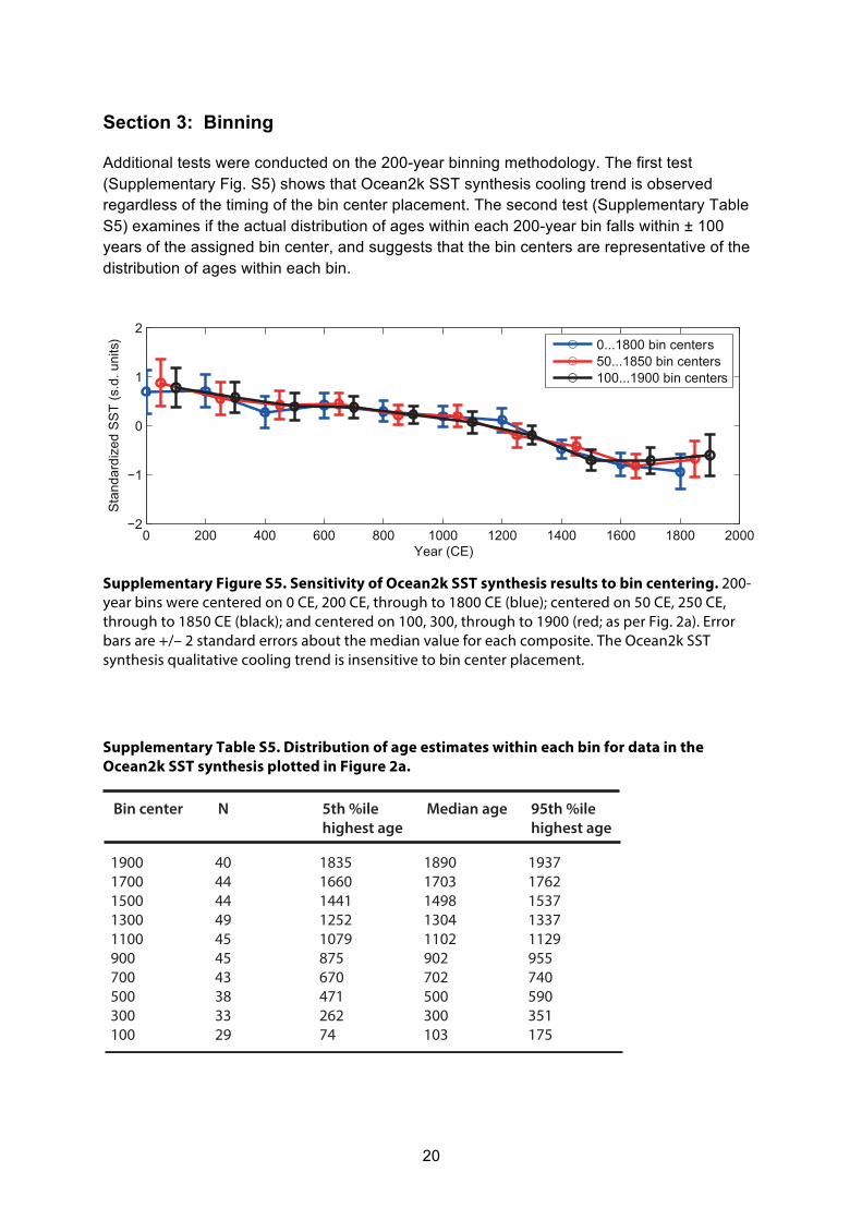
Additional tests were conducted on the 200-year binning methodology. The first test (Supplementary Fig. S5) shows that Ocean2k SST synthesis cooling trend is observed regardless of the timing of the bin center placement. The second test (Supplementary Table S5) examines if the actual distribution of ages within each 200-year bin falls within ± 100 years of the assigned bin center, and suggests that the bin centers are representative of the distribution of ages within each bin.

Supplementary Figure S5. Sensitivity of Ocean2k SST synthesis results to bin centering. 200-year bins were centered on 0 CE, 200 CE, through to 1800 CE (blue); centered on 50 CE, 250 CE, through to 1850 CE (black); and centered on 100, 300, through to 1900 (red; as per Fig. 2a). Error bars are +/– 2 standard errors about the median value for each composite. The Ocean2k SST synthesis qualitative cooling trend is insensitive to bin center placement.

Supplementary Table S5. Distribution of age estimates within each bin for data in the Ocean2k SST synthesis plotted in Figure 2a.

0 200 400 600 800 1000 1200 1400 1600 1800 2000!2

!1

0

1

2

Stan

dard

ized

SST

(s.d

. uni

ts)

Year (CE)

0...1800 bin centers50...1850 bin centers100...1900 bin centers

Supplementary Table XX. Distribution of age estimates within each bin for observationsin the data composite plotted in Fig 2a. By de!nition of the binned composite, ages must fall within ± 100 years of each bin center, but the median and percentile estimates suggest that the bin centers are representative of the distribution of ages within each bin.

1900 40 1835 1890 19371700 44 1660 1703 17621500 44 1441 1498 15371300 49 1252 1304 13371100 45 1079 1102 1129900 45 875 902 955700 43 670 702 740500 38 471 500 590300 33 262 300 351100 29 74 103 175

Bin center N 5th %ile Median age 95th %ile highest age highest age

21

Section 4: Standardization

Alternatives to standardization: Calibration of the Ocean2k SST synthesis

It is useful to consider the Ocean2k SST trend in temperature units, in order to estimate parameters such as ocean heat storage and global climate sensitivity. However, if we were to take the SST reconstructions as originally published, assigned the data into 200-year bins and combined these directly without standardizing we would introduce significant biases because the 57 input reconstructions are not distributed evenly amongst the ocean basins, nor across latitudes, and the reconstructions have vastly different absolute SSTs. Hence, when combined, the Ocean2k synthesis trend in temperature units would be skewed toward regions with a larger number of reconstructions. Furthermore, combining binned absolute SSTs may introduce biases, for example, simply due to differences in the calibrations used in the original publications.

To circumvent issues related to directly combining SST reconstructions, ideally we would take the Ocean2k SST synthesis (based on the 200-year binned and standardized reconstructions) and calibrate it against the historical, observed instrumental SST data, to derive an Ocean2k SST synthesis presented in temperature units. However, the 200-year binning and the absolute dating errors on the reconstructions precludes direct calibration against the ~150 years of instrumental SST data. Instead, we use two alternative methods to determine the Ocean2k SST temperature units:

1) The average anomaly method, which is also described in the ‘Are estimates of the linear cooling trend dependent on standardization?’ section below. Each of the 57 SST reconstructions was averaged at 200-year resolution. The mean of each reconstruction thus averaged was then subtracted (i.e. reconstructions were centered) to produce 57 anomaly time series, with units of degree Celsius anomaly. The 57 anomaly time series were averaged to produce a global mean anomaly trend estimate (Supplementary Tables S6 and S7; herein termed ‘average anomaly’). We also calculated the average anomaly by first weighting each anomaly time-series by it’s ocean basin area, before averaging (Supplementary Table S6).

2) The space-for-time method, in which we take advantage of the spatial distribution of our SST reconstructions, in that they span a range of SSTs (i.e. cold SSTs at the high latitudes and warm SSTs at the low latitudes). Consequently, we are able to substitute a spatial distribution of SST for a temporal distribution of SSTs. We regress the 1801–2000 average reconstructed SST at each of 42 sites with 1801–2000 bin average values against the climatological SST for the corresponding closest grid point in the World Ocean Atlas (Locarnini et al., 2010):

Ocean2k SST = a + b*Climatological SST + epsilon (ε)

22

The 42 reconstructed SSTs were plotted against the 42 climatological SSTs (Supplementary Fig. S6a) and the data were used to calculate a calibration. We bootstrapped 1000 estimates of the calibration and its RMS error by randomly selecting 21 of 42 sites with replacement, estimating the linear regression of Ocean2k SST on climatological SST, predicting the reconstructed SST at locations not used to produce that regression estimate, and averaging the squared residuals of the predicted minus actual Ocean2k SST values. The median (5th percentile, 95th percentile) of these estimated ‘space-for-time’ regressions was:

Ocean2k SST = 0.97(–0.25, 2.08) + 0.96(0.91, 1.01)*climatological SST

Note that the intercept is not significantly different from zero, and the slope is not significantly different from unity, suggesting that the synthesis of independent site-level SST reconstructions is a one-to-one mapping from climatological SST (Supplementary Fig. S6a). Nevertheless, we inverted the regression of Ocean2k SST anomaly on climatological SST anomaly to produce SST estimates consistent with those obtained from gridded direct SST observations (Supplementary Fig. S6 b,c; Supplementary Table S6).

For both methods we compute the anomalies relative to the climatological global mean area-weighted SST from the World Ocean Atlas (18.61°C; Locarnini et al., 2010).

We then calculate the anomaly trend (5th, 95th percentile standard error), in units of °C per thousand years (°C/kyr), by bootstrapped resampling with replacement of the regression of SST anomaly versus time (Methods; Supplementary Table S6; as in Fig. 3). We also calculate bootstrapped area-weighted regression slope. Our best estimate of the SST cooling trend, scaled to temperature units using the average anomaly method (method 1), for the periods 1–2000 CE is –0.3°C/kyr to –0.4°C/kyr, and for 801–1800 CE is –0.4°C/kyr to –0.5°C/kyr. The space-for-time method regression (method 2) produces a trend estimate in either interval that has a slope about 0.1°C larger (Supplementary Table S6). Bootstrapped area-weighted regression slopes indistinguishable within uncertainty of the unweighted regression slopes for both temperature anomaly calculation method.

Because anomaly composites are likely to be biased by uneven sampling of regions with different SST variances, we primarily discuss global composites of standardized data. However, anomaly estimates are valuable because they retain temperature units and thereby additional physical interpretability.

23

Supplementary Figure S6. Estimate of SST anomalies using the space-for-time calibration. a. Space-for-time regression bootstrap estimates (blue) and SST data (red) for the Ocean2k 1801–2000 bin values (N=42) vs. closest climatological grid point values from Locarnini et al. (2010). The 1:1 line is given (thick black line). Calibration equation and regression statistics are given in Supplementary Section 4. b. Slope estimates (blue) and median slope estimate (black) for space-for-time calibrated Ocean2k SST anomaly, for 0–2000 CE, calculated as in Figure 3, but over the longer time interval. Median slope and probability of a negative slope (cooling trend; p(slope<0)) are shown. c. Slope estimates (blue) and median slope estimate (black) for space-for-time calibrated Ocean2k SST anomaly, for 801–1800 CE, calculated as in Figure 3. Median slope and probability of a negative slope (cooling trend; p(slope<0)) are shown.

24

Supplementary Table S6. Ocean2k SST anomaly trend for 1-2000 CE and 801-1800 CE, estimated using the two methods described in the Supplementary Section 4. The numbers in parentheses are for the area-weighted average anomaly estimates.

Average anomaly 1-2000 -0.31 (-0.32) 0.87 (0.86)

Space for time 1-2000 -0.38 (-0.39) 0.87 (0.87)

Average anomaly 801-1800 -0.42 (-0.40) 0.83 (0.81)

Space for time 801-1800 -0.54 (-0.53) 0.81 (0.80)

Method Interval (CE) Median slope p(slope<0) (°C/ky)

25

Are estimates of the linear cooling trend dependent on standardization?

In the Ocean2k SST synthesis each time series, derived either from paleoclimate archives or from model simulations, is averaged to one value per 200-year interval (200-year binning). Each time series is then standardized by subtracting its mean and dividing the residual by its standard deviation. The mean and the standard deviation are calculated over a reference period of 801–1800 CE for the model simulations, and for the reconstruction length for the paleoclimate time series. This standardization method permits the compositing of time series (model or measured) from regions with very different temperature variances in order to estimate a standardized global mean SST anomaly.

However, the use of standardization represents another potential source of bias within this study. To assess the robustness of our fundamental conclusions with regard to standardization, we calculated trends for 1) anomalies (i.e. mean subtracted from the binned time series) and 2) variance-standardized anomalies (i.e. the standardization method described above), for the following composites:

A. Multi-model composite simulations, 801–1800 CE (Supplementary Table S7)

B. Ocean2k SST synthesis, 1–2000 CE (Supplementary Table S7)

C. Ocean2k SST synthesis, 801–1800 CE (Supplementary Table S7)

D. LOVECLIM individual and combined forcing simulations, where each experiment comprises a 10-member ensemble, 851–1800 CE (Supplementary Table S8)

E. CSIRO Mk3L cumulative forcing 3-member ensembles, 801–1800 CE (Supplementary Table S9)

The number of data points per bin for the Ocean2k SST synthesis anomaly and standardized anomaly calculations are given in Supplementary Table S10.

For either the 1–1800 CE or 801–1800 CE interval, the probability of a negative Ocean2k SST synthesis anomaly slope (p(slope<0)) is unchanged relative to that for standardized data (Supplementary Table S7). The same is true for the multi-model, LOVECLIM, and CSIRO Mk3L composites (Supplementary Tables S7–S9), suggesting that biases arising from the use of standardization do not affect the fundamental conclusions of this study.

For the LOVECLIM individual forcing simulations, the magnitudes of the simulated slopes are less than for the Ocean2k SST synthesis (Supplementary Table S8 compared to Supplementary Table S7). As a result, the probabilities of a cooling trend are also lower, but for all LOVECLIM experiments, results for cooling trend probabilities are not sensitive to standardization. When all forcings are applied, the probabilities exceed those for the Ocean2k synthesis and probabilities become comparable to those for the multi-model composite. The results for the CSIRO Mk3L simulations are similar (Supplementary Table S9). Both the magnitude of the simulated slope and the probability that the slope is negative increase as individual forcings are progressively added to the model, and again the results are not sensitive to standardization.

26

A note on paleoclimate data and model simulation anomaly SST trend amplitudes

The cooling trends within the Ocean2k SST synthesis and multi-model composite have two origins: 1) internal variability, and 2) the forced signal. The trend in the Ocean2k SST synthesis includes uncertainties associated with the indirect estimation of SST from paleoclimate data, including both amplitude and chronological uncertainties. The multi-model composite also includes uncertainties associated with model physics and the magnitude of the prescribed forcings. These uncertainties may cause the Ocean2k SST synthesis or multi-model composite to overestimate or underestimate the amplitudes of internal variability and the forced signal. Standardization normalizes the different estimates of the variability, so the median 801–1800 CE cooling trend observed in the Ocean2k SST composite (–1.49 s.d. units/ky) is similar to that observed (–1.85 s.d. units/ky) in the PMIP3-compliant multi-model composite (Supplementary Table S7). However, without variance normalization (Supplementary Table S7), the corresponding observed anomaly cooling trend (–0.41 °C/ky) is within the range of estimated surface cooling trends from terrestrial regions (PAGES 2k Consortium, 2013). This is three times larger than the multi-model composite anomaly cooling trend (–0.12 °C/ky; all anomaly values from Supplementary Table S7). Further research is needed to reconcile these anomaly differences, so that detailed quantitative and mechanistic analyses of the underlying processes may be pursued.

27

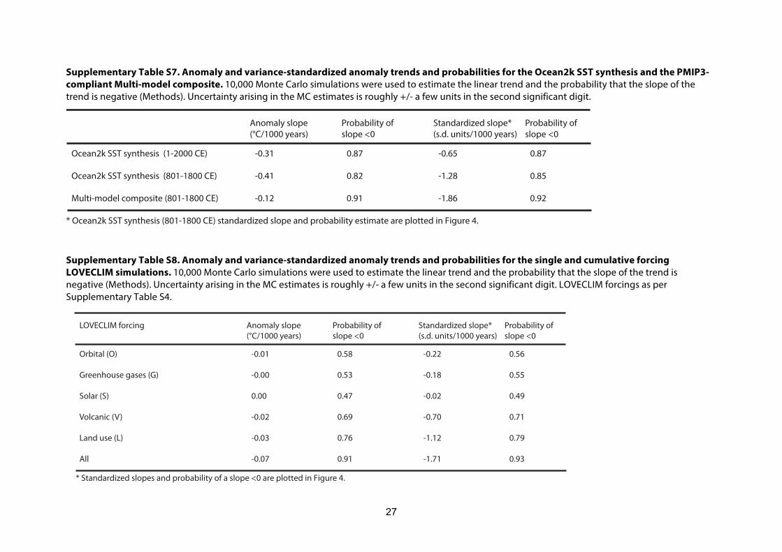
Supplementary Table S7. Anomaly and variance-standardized anomaly trends and probabilities for the Ocean2k SST synthesis and the PMIP3-compliant Multi-model composite. 10,000 Monte Carlo simulations were used to estimate the linear trend and the probability that the slope of the trend is negative (Methods). Uncertainty arising in the MC estimates is roughly +/- a few units in the second significant digit.

Supplementary Table S8. Anomaly and variance-standardized anomaly trends and probabilities for the single and cumulative forcing LOVECLIM simulations. 10,000 Monte Carlo simulations were used to estimate the linear trend and the probability that the slope of the trend is negative (Methods). Uncertainty arising in the MC estimates is roughly +/- a few units in the second significant digit. LOVECLIM forcings as per Supplementary Table S4.

Supplementary Table S7. Anomaly and variance-standardized anomaly trends and probabilities for the Ocean2k SST synthesis and the Multi-model composite. 10,000 Monte Carlo simulations were used to estimate the linear trend and the probability that the slope of the trend is negative (Methods). Uncertainty arising in the MC estimates is roughly +/- a few units in the second signi!cant digit.

* Ocean2k SST synthesis (801-1800 CE) standardized slope and probability estimate are plotted in Figure 4.

Ocean2k SST synthesis (1-2000 CE) -0.31 0.87 -0.65 0.87

Ocean2k SST synthesis (801-1800 CE) -0.41 0.82 -1.28 0.85

Multi-model composite (801-1800 CE) -0.12 0.91 -1.86 0.92

Anomaly slope Probability of Standardized slope* Probability of (°C/1000 years) slope <0 (s.d. units/1000 years) slope <0

* Standardized slopes and probability of a slope <0 are plotted in Figure 4.

Orbital (O) -0.01 0.58 -0.22 0.56

Greenhouse gases (G) -0.00 0.53 -0.18 0.55

Solar (S) 0.00 0.47 -0.02 0.49

Volcanic (V) -0.02 0.69 -0.70 0.71

Land use (L) -0.03 0.76 -1.12 0.79

All -0.07 0.91 -1.71 0.93


LOVECLIM forcing

28

Supplementary Table S9. Anomaly and variance-standardized anomaly trends and probabilities for the cumulative forcing CSIRO Mk3L simulations. 10,000 Monte Carlo simulations were used to estimate the linear trend and the probability that the slope of the trend is negative (Methods). Uncertainty arising in the MC estimates is roughly +/- a few units in the second significant digit. CSIRO Mk3L forcings as per Supplementary Table S4.

Supplementary Table S10. SST reconstruction values available per 200-year bin. N for standardized SST in some cases is < N for anomaly SST because for data series available for only one bin within the analysis interval, a variance cannot be calculated. For the anomaly calculation if a data series has only one bin in the analysis interval then a mean can still be calculated and a variance is not needed. Bin center (CE) 1–2000 CE 1–1800 CE N for anomaly SST N for standardized SST N for anomaly SST N for standardized SST 100 29 29 - - 300 33 33 - - 500 38 38 - - 700 43 43 - - 900 45 45 45 44 1100 45 45 45 45 1300 49 49 49 49 1500 44 44 44 44 1700 44 44 44 40 1900 42 40 - -

* Standardized slopes and probability of a slope <0 are plotted in Figure 4.

O -0.01 0.57 -0.13 0.53

OG -0.01 0.58 -0.30 0.60

OGS -0.02 0.62 -0.62 0.67

OGSV -0.12 0.94 -2.08 0.95


CSIRO Mk3L forcing

29

Section 5: Testing if the Ocean2k synthesis network is representative of global SST on 200-year time scales

Methods for correlation map in Figure 1

In Figure 1, the grid point SST in a given model was correlated with the model's global mean SST for six individual models, where the simulation data were binned into 200-year intervals. Then the six model correlation fields were appended into a single ArcGIS (v.10) GRID file, and a 2-D localized second-order polynomial interpolation method (with an exponential kernel and a required range of between 10 to 1,000 data points) was applied to generate a smoothed contour map (with error statistics), to account for the range of model grid resolutions. For model SST outputs that occupied the same latitude/longitude nodes, a single mean was calculated prior to contouring. The significance of the correlations in Figure 1 cannot be quantified because the degrees of freedom (df=3) are too small to assess correlation significance reliably, but the distribution of correlations suggests that at bicentennial resolution, SST variations over the global domain mirror the global mean.

Complementing Figure 1 is Supplementary Figure S7, which compares each individual model global mean SST with 1) a composite of the model grid points matched to the 57 Ocean2k SST synthesis locations, temporal extent, and seasonality (Figure 1; Supplementary Table S1), and 2) as for 1) but with the additional step for weighting the 57 locations to their ocean basin area (see also sub-section ‘Weighting the SST synthesis for ocean basin area’ and Supplementary Table S11 for weighting). The models have varying spatial resolutions, but at 200-year intervals they capture the primary processes likely to influence our reconstruction. Qualitative agreement between models global mean SST, area-weighted, and non-weighted composites suggests that for centennial time scales, the 57-site Ocean2k network provides approximately the same information as the true global estimate.

30

Supplementary Figure S7. Climate model estimates of the potential bias due to the non-homogeneous spatial and temporal distribution of the 57 Ocean2k reconstructions. Blue curves give 200-year standardized averages of simulated SST masked for the space-time availability of the Ocean2k reconstructions (temperature in s.d. units), and for the response season for each location (as reported in the original publications and documented in Supplementary Table S1). Note that standardization occurs after averaging to the 200-year bins (see Methods). Green curves are the same as the blue curves, except that they are area-weighted estimates, whereby the 57 locations were weighted by their respective ocean basin area (ocean basin area weighting given in Supplementary Table S11). Red curves are area-weighted 200-year standardized average values over all model SST grid points. Labels above each plot refer to the individual models and simulation details that are given in Supplementary Table S4. There is qualitative agreement between the averages masked for the space-time availability of the Ocean2k 57 reconstructions and the true global means, which suggests that our 57-site network, at 200-year resolution, is representative of the true global estimate.

Tem

pera

ture

(s.d

. uni

ts)

Tem

pera

ture

(s.d

. uni

ts)

Year (CE) Year (CE) Year (CE)

900 1100 1300 1500 1700!2

!1

0

1

2

900 1100 1300 1500 1700!2

!1

0

1

2

900 1100 1300 1500 1700!2

!1

0

1

2

900 1100 1300 1500 1700!2

!1

0

1

2

BCC-CSM1-1 CCSM4 FGOALS-s2

LOVECLIM MPI-ESM CSIRO Mk3L

900 1100 1300 1500 1700!2

!1

0

1

2

900 1100 1300 1500 1700!2

!1

0

1

2

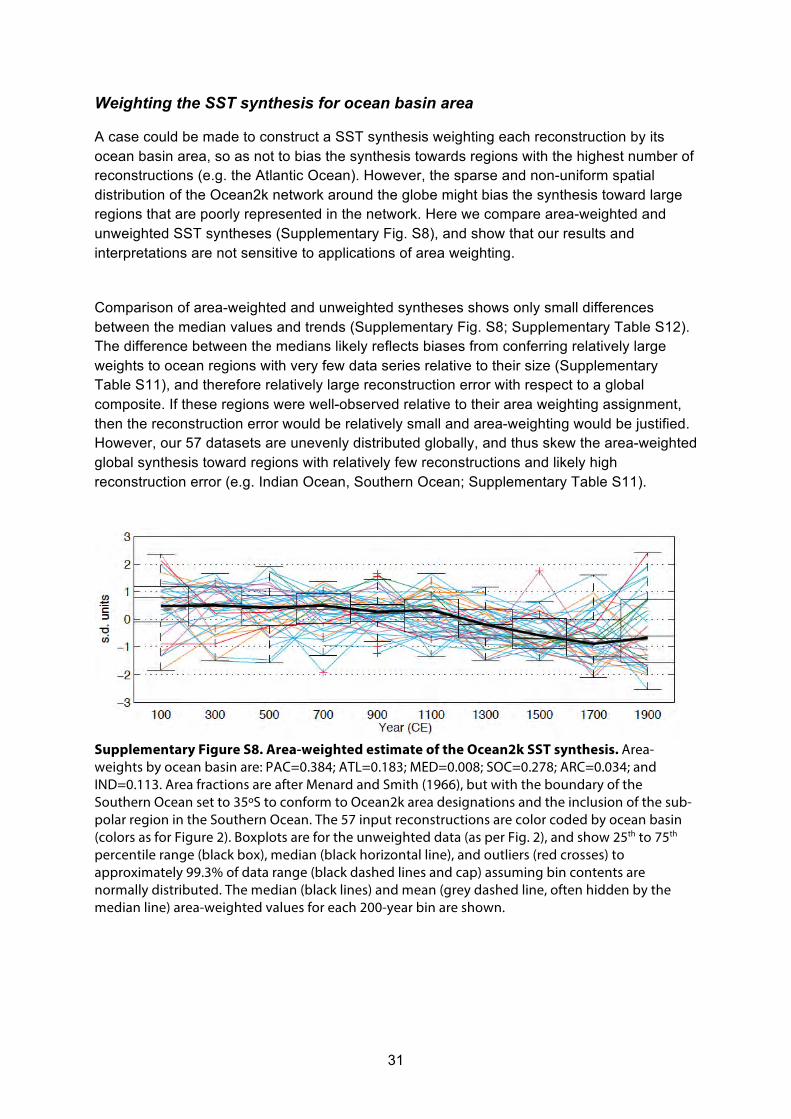
31

Weighting the SST synthesis for ocean basin area

A case could be made to construct a SST synthesis weighting each reconstruction by its ocean basin area, so as not to bias the synthesis towards regions with the highest number of reconstructions (e.g. the Atlantic Ocean). However, the sparse and non-uniform spatial distribution of the Ocean2k network around the globe might bias the synthesis toward large regions that are poorly represented in the network. Here we compare area-weighted and unweighted SST syntheses (Supplementary Fig. S8), and show that our results and interpretations are not sensitive to applications of area weighting.

Comparison of area-weighted and unweighted syntheses shows only small differences between the median values and trends (Supplementary Fig. S8; Supplementary Table S12). The difference between the medians likely reflects biases from conferring relatively large weights to ocean regions with very few data series relative to their size (Supplementary Table S11), and therefore relatively large reconstruction error with respect to a global composite. If these regions were well-observed relative to their area weighting assignment, then the reconstruction error would be relatively small and area-weighting would be justified. However, our 57 datasets are unevenly distributed globally, and thus skew the area-weighted global synthesis toward regions with relatively few reconstructions and likely high reconstruction error (e.g. Indian Ocean, Southern Ocean; Supplementary Table S11).

Supplementary Figure S8. Area-weighted estimate of the Ocean2k SST synthesis. Area-weights by ocean basin are: PAC=0.384; ATL=0.183; MED=0.008; SOC=0.278; ARC=0.034; and IND=0.113. Area fractions are after Menard and Smith (1966), but with the boundary of the Southern Ocean set to 35ºS to conform to Ocean2k area designations and the inclusion of the sub-polar region in the Southern Ocean. The 57 input reconstructions are color coded by ocean basin (colors as for Figure 2). Boxplots are for the unweighted data (as per Fig. 2), and show 25th to 75th percentile range (black box), median (black horizontal line), and outliers (red crosses) to approximately 99.3% of data range (black dashed lines and cap) assuming bin contents are normally distributed. The median (black lines) and mean (grey dashed line, often hidden by the median line) area-weighted values for each 200-year bin are shown.

32

Supplementary Table S11. Comparison of fraction of reconstructions from a given ocean basin (N_region/57) to area weighting (Menard and Smith, 1966, modified). Note that decimal place is retained only so that fractions sum to 100%. Ocean (regional N)/57 (%) Area weight (%) Pacific 28.1 38.4 Atlantic 50.9 18.3 Mediterranean 7.0 0.8 Southern Ocean 7.0 27.8 Arctic 3.5 3.4 Indian 3.5 11.3

Supplementary Table S12. Comparison of trend statistics for the Ocean2k SST synthesis and an area-weighted SST composite. For the area-weighted composite ordinary least squares linear regression was performed by minimizing the weighted least squared errors in the predicted values for each site. Each reconstruction was weighted by its ocean basin area as given in Supplementary Table S11. Mean

standardized slope (s.d.

units/1000 years)

Median standardized

slope (s.d. units/1000 years)

95% confidence

interval

Probability of slope <0

Ocean2k SST synthesis (1-2000 CE; unweighted)

-0.63 -0.65 -1.67, 0.50 0.87

Area-weighted composite (1-2000 CE)

-0.66 -0.69 -1.72, 0.61 0.86

We construct our synthesis on the basis that at 200-year resolution, any one location is an independent indicator of the global average, that is, there is no a priori reason to state that one single record in one ocean basin is more representative of the global mean or even of the mean at the basin scale than any other record. Therefore the synthesis with no area-weighting should give us the best estimate of the true global median at these timescales (Fig. 1). This reasoning is consistent with the tests made using model results (Supplementary Fig. S7). In the models the true (model) standardized global SST mean can be estimated because of global coverage of model output. The SST data for the 57 Ocean2k sites are extracted from each model simulation and a composite made, which, by comparison with the true standardized global SST mean, shows that the Ocean2k space-time reconstruction network is a suitable estimate of the true standardized SST global mean (Supplementary Fig. S7). Since we only make inferences on reconstructions at the global scale, we consider that an unweighted median is our best estimate of standardized global SST.

Although we do not area-weight our synthesis based on the 57 input data series, we note too that area-weighted syntheses may be more appropriate once more reconstructions are available from under-sampled regions, and for when investigating variability on <200-year time scales.

33

Section 6: Sensitivity tests

Sources of bias and error in SST reconstructions

Estimates of past SST based on marine archives have associated uncertainties and the potential for bias in the signal they record (Masson-Delmotte et al., 2013). The following discussion outlines the use of, and key issues with, SST reconstructions that contribute to the Ocean2k SST synthesis. The Ocean2k SST synthesis acknowledges that the global SST reconstruction is subject to these sources of bias, and the 57 input datasets were subsampled as best as possible to test if the global cooling trend was a function of one of these biases (Fig. 2b). All bias tests (Fig. 2b) demonstrate that the cooling trend is robust.

C37 alkenones unsaturation index

The C37 alkenones unsaturation index (UK'37 ) uses long-chain unsaturated ketones

(alkenones) photosynthesized primarily by the coccolithophorids Emiliania huxleyi and Gephyrocapsa oceanica that thrive in the upper ocean. Most reconstructions used in the Ocean2k SST synthesis use the calibration of (Prahl et al., 1988) based on the empirical linear relationship obtained from laboratory cultures to translate UK'

37 into SST (Supplementary Table S1) following the recommendations of (Prahl et al., 2000). Other studies use different calibrations that provide similar results (Supplementary Table S1).

UK'37 in sediments is thought to reflect mean annual SST (Müller et al., 1998; Conte et al.,

2006), however if the coccolithophorid production (or bloom) occurs in a particular month or season (Sicre et al., 1999; Bijma et al., 2001; Leduc et al., 2010b; Prahl et al., 2010; Schneider et al., 2010; Sicre et al., 2011; Lohmann et al., 2013), then SST estimates may be skewed towards that season, diverging from the mean annual value, and a seasonal bias may be introduced. In sub-polar regions, the presence of sea-ice can also delay the season of alkenone production (Sicre et al., 2014). An additional bias in reconstructing SST may arise from subsurface production of coccolithophorids growing in or below the thermocline rather than at the sea surface (see e.g. Ternois et al., 1996; Andruleit et al., 2003).

Lateral advection of “detrital” alkenones by strong surface currents in some regions may be another source of bias. Advected alkenones can indeed overwhelm the local SST signal in extremely low productivity waters (Sicre et al., 2005; Conte et al., 2006; Rühlemann and Butzin, 2006). Sediment re-suspension and long-distance advection of alkenones by bottom currents may also alter the sedimentary SST signal through deposition of remotely produced alkenones (Ohkouchi et al., 2002; Mollenhauer et al., 2003; Mollenhauer et al., 2005). Given the large number of alkenone-based SST records in the Ocean2k SST synthesis, such influences in an individual record are unlikely to alter the overall trend in the composite.

34

In addition to standardizing reconstructions, we test, where we can, for these potential biases with our ‘seasonality’ sensitivity test, and by comparing the trend in alkenone-only reconstructions with the Mg/Ca-only and other reconstructions (Fig. 2b). We also plot the reconstructions where more than one reconstruction exists from the same site (Supplementary Fig. S3). We conclude that absolute temperatures differ but the trends are in general similar.

Mg/Ca in foraminifera

Laboratory, core-top, and sediment trap studies suggest that Mg/Ca in planktic foraminifera increases exponentially with increasing temperature of calcification (Dekens et al., 2002; Anand et al., 2003; Martínez-Botí et al., 2011). The Mg/Ca-based SST records included in our study use these calibrations (e.g. Supplementary Table S1). However, there are several potential biases that may influence Mg/Ca-based SST reconstructions.

First, core-top calibrations vary between ocean basins (e.g. McConnell and Thunell, 2005). While earlier work suggests a strong salinity bias at salinities greater than 35 (Bender et al., 1975; Nürnberg et al., 1996; Lea et al., 1999; Kısakürek et al., 2008; Mathien-Blard and Bassinot, 2009; Arbuszewski et al., 2010) more recent work suggests that the salinity bias is smaller than originally thought, and that departures from mean annual SST are due to dissolution in deep sites and varying seasonality and depth habitat of planktic foraminifera with latitude (Hönisch et al., 2013). For most species and locations, it is assumed that Mg/Ca-based SST reconstructions represent mean annual conditions, implying that the flux of foraminiferal specimens to the sediment core site is approximately constant throughout the year. However, there is considerable evidence from sediment trap studies that the flux of Globigerinoides ruber, the mixed-layer dwelling foraminifera most commonly used for tropical and subtropical Mg/Ca-based SST reconstructions, can be seasonally biased, often favoring times of higher productivity (Thunell et al., 1983; Deuser, 1987; Sautter and Thunell, 1991; Curry et al., 1992; Kawahata et al., 2002; Eguchi et al., 2003; Tedesco and Thunell, 2003; Mohtadi et al., 2009). Unfortunately, there are few studies that use sediment traps to evaluate the seasonal flux of foraminifera to the seafloor from non-upwelling regions, and it is not straightforward to estimate the likely seasonality on an individual basis. In this synthesis, we indicate if the Mg/Ca-based SST reconstruction records annual mean or SST for a particular season, as reported in the original publication of the dataset (Supplementary Table S1). Our analysis of model simulation SSTs for our Ocean2k SST locations suggests that seasonal trends in SST are generally similar to annual mean trends (Supplementary Fig. S7), and are unlikely to introduce significant biases in our synthesis.

Post-depositional dissolution may also influence Mg/Ca-based SST estimates. Core-top studies show that calcite dissolution may preferentially remove high-Mg calcite and thus result in an underestimation of SST. Calibrations have been developed to correct for this effect below 1600 m in the Pacific Ocean, but a correction in the Atlantic may not be necessary due to a high carbonate saturation state (e.g. Dekens et al., 2002). Only two Pacific Mg/Ca-based SST reconstructions were from cores retrieved from deeper sites (Supplementary Table S1) but a depth-dependent calibration was considered unnecessary

35

by the original authors, and indeed, core-top SST estimates are similar to modern values. While the carbonate saturation state of the deep ocean may change on longer time scales, on the time scale considered in this study, it probably did not change appreciably at most sites, and depth-dependent calibrations have not been applied.

Finally, Mg/Ca in foraminifera may also be affected by clay contamination or may be modified during sample preparation, and laboratory preparation procedures have been developed to minimize such contamination and analytical artifacts (Barker et al., 2003; Klinkhammer et al., 2004).

Where possible we test for such potential biases using our ‘seasonality’ and ‘water depth’ sensitivity tests (Fig. 2b), and by comparing the Mg/Ca-only reconstructions with other reconstructions (Fig. 2b). Where more than one reconstruction exists from the same site, these are all plotted for comparison (Supplementary Fig. S3). These show that absolute temperatures differ but the trends are in general similar.

TEX86

The TEX86 paleothermometer is based on membrane lipids from Crenarchaeota (Schouten et al., 2002; Kim et al., 2010), specifically, the relative proportion of different Glycerol Dialkyl Glycerol Tetraethers (GDGTs) containing varying amounts of cyclopentane rings (Schouten et al., 2002). SSTs are derived from the TEX86 through a linear empirical relationship (Schouten et al., 2002), and a recent extension of the global core-top calibration using modified calibration curves has produced more realistic SST estimates for both warm and cold temperature ranges (Kim et al., 2010). Overall, knowledge on the depth of production of GDGTs is a major limitation for improving temperature estimates from this proxy.

Two sedimentary SST reconstructions based on TEX86 are included in the Ocean2k SST synthesis. The first is from ODP Site 1098 off the Antarctica Peninsula. To assess the applicability of the TEX86 thermometer in the region, TEX86 values were obtained from seven surface sediment samples. The regional core top SST estimates align along the global calibration of Kim et al., (2008) if local spring/summer SSTs are used (Shevenell et al., 2011). The second TEX86 SST reconstruction is based on sediment from ODP Hole 1202B, southern Okinawa Trough (Wu et al., 2012) and uses the calibration of Kim et al., (2012).

With only two TEX86 reconstructions it is difficult to test for bias specifically related to this reconstruction type, however the TEX86 reconstructions show a cooling trend similar to the other reconstruction types (Fig. 2b).

36

Sr/Ca in coral

The Sr/Ca ratio in coralline aragonite is negatively correlated with ocean temperature (Weber, 1973; Smith et al., 1979). Sr/Ca SST calibrations equations differ between locations and species, and in some cases between corals of the same species from the same reef (see review in Corrège, 2006). The reason for these offsets is not fully understood but have been alternatively attributed to Rayleigh fractionation and crystal growth rates (McConnaughey, 1989a, b; Cohen et al., 2001; Gaetani et al., 2011), coral growth rates and symbiont photosynthesis (e.g. de Villiers et al., 1994; Gagan et al., 2012), differences in seawater Sr/Ca (de Villiers et al., 1994) or laboratory offsets (Hathorne et al., 2013). Post-depositional diagenesis of the coral skeleton may also contribute to errors in SST estimates (Enmar et al., 2000; Müller et al., 2001; McGregor and Gagan, 2003; Cohen and Hart, 2004; Hendy et al., 2007; Hathorne et al., 2011).

The Ocean2k SST synthesis includes the Great Barrier Reef (GBR) Sr/Ca-based SST estimate from Porites corals; the most commonly used tropical Pacific coral for paleoclimate reconstruction. This reconstruction is the average Sr/Ca of eight individual corals, where ‘bulk’ 5-year resolution samples were milled and analyzed from each coral. The ‘master’ GBR Sr/Ca reconstruction from the 8 corals reduces the likelihood of biases due to the potential issues described above, and the individual records share, on average, 33% of common variance with the ‘master’ record (Hendy et al., 2002). The Hendy et al., (2002) ‘master’ GBR Sr/Ca record is publically archived as an uncalibrated dataset; we apply the calibration slope of Alibert and McCulloch (1997) to convert Sr/Ca to SST, as done in the original publication (Hendy et al., 2002).

With only one coral Sr/Ca SST reconstruction it is difficult to test for bias specifically related to this reconstruction type, however the coral reconstruction shows a cooling trend similar to the other reconstruction types (Fig. 2b). The coral reconstruction is unlikely to contain seasonality bias. Note too that the coral reconstruction was included in the ‘sedimentation rate’ sensitivity test, where we take coral growth rate to be equivalent to a marine core sedimentation rate.

Dinoflagellate cysts

The relative abundances of organic-walled dinoflagellate cysts (dinocysts) are used to reconstruct SST, particularly in high-latitude marine environments. In contrast to siliceous or carbonate microfossils, dinocysts are generally well preserved in sediments affected by dissolution because they are composed of highly resistant refractory organic matter (de Vernal et al., 2001). An extensive database on modern dinocyst distribution versus environmental parameters defines modern analogues and thus allows the reconstruction of past SST (de Vernal et al., 2013). One SST reconstruction based on dinocyst abundances was included in the Ocean2k SST synthesis. This SST reconstruction, from the Fram Strait (Bonnet et al., 2010), was generated using the Northern Hemisphere reference core-top database and the modern analogue technique (MAT). This method is based on the degree of similarity between fossil and modern species and assumes fossil assemblages developed in

37

environmental conditions that are similar to their modern analogues (Guiot, 1990). It allows for separate reconstructions of summer, winter and annual SST. The main uncertainty of the method is that surface samples may average as much as a few hundred years of sedimentation, whereas reference SST data derived from instrumental observations represent the most recent decades only (de Vernal et al., 2008). A second uncertainty, which may at times arise, is the existence of non-analogue scenarios, in which case SST may not be calculated (e.g. Solignac et al., 2011), although this is uncommon for the past 2000 years.

With only one dinocyst reconstruction it is difficult to test for bias specifically related to this reconstruction type, however it shows a cooling trend similar to the other reconstruction types (Fig. 2b).

Planktic foraminifera

Planktic foraminifera are found in a wide range of temperature conditions from tropical to polar regions. They are generally restricted to bathyal or to outer shelf areas (Bé, 1977; Hemleben et al., 1989), although they may be advected into near-shore and fjord settings with currents (e.g. Seidenkrantz, 1993; Andresen et al., 2013).

Planktic foraminifera were among the first organisms for which transfer functions were developed (Imbrie, 1971; Kucera et al., 2005), and a number of different transfer function methods are used on planktic foraminiferal assemblages (Kucera et al., 2005). These all take advantage of a large database of modern foraminiferal distribution in surface sediments (Pflaumann et al., 2003; Kucera et al., 2005). However, the same non-analogue issues exist as for the dinoflagellate cysts, and the database of the modern planktic faunal distribution is likewise based on core tops and surface sediments that may encompass deposits covering several hundreds of years.

It is worth mentioning that because planktonic foraminifera are protozoa and as such not directly dependent on photosynthesis, they are not solely restricted to the photic zone. Although highest concentrations of foraminifera are found between 10–50 m depth in the water column, the depth habitat of planktonic foraminifera varies from species to species (Bé, 1977; Hemleben et al., 1989). Consequently, planktonic foraminifera do not necessarily reconstruct true surface-water conditions and may in large parts of the ocean in fact be more sensitive to subsurface temperatures (Telford et al., 2013).

The Ocean2k dataset includes two SST reconstructions based on assemblages of planktic foraminifera, both from the Atlantic Ocean (deMenocal et al., 2000; Spielhagen et al., 2011). Core MSM5/5-712 from the eastern Fram Strait represents a site influenced by the northward flow of Atlantic water, and the record thus tracks the strength and temperature of Atlantic water flow to the Arctic ocean (Spielhagen et al., 2011). SSTs were calculated using the SIMMAX modern analogue technique (Pflaumann et al., 2003), which reconstructs temperatures at 50 m water depth.

38

ODP Leg 108, Hole 658C from off northwest Africa is situated in the boundary zone between cold temperate and subtropical waters. SST was reconstructed using the F13’ transfer function and a modern database of planktic foraminiferal faunas from 191 Atlantic core tops (deMenocal et al., 2000). Both cold and warm season SSTs were reconstructed and for the Ocean2k synthesis, we averaged cold and warm season estimates in order to obtain an average annual SST record.

With only two planktic foraminiferal reconstructions it is difficult to test for bias specifically related to this reconstruction type, however similar to the other reconstruction types it shows a general cooling trend (Fig. 2b). We plot all SST reconstructions where more than one reconstruction exists from the same site (Supplementary Fig. S3); this shows similar trends despite some difference in absolute temperatures.

Generic sources of bias and error

The uncertainty in estimating SST from measurements made on marine archives includes analytical, observational and reconstruction errors. There is analytical uncertainty associated with all measurements; age modeling of discontinuous layered and/or bioturbated marine archives may diffuse and/or translate the signal in depth and therefore in time. In addition, observational uncertainty may arise from the imperfectly understood response of the indicator to SST variation, biological mediation of the measurement (so-called vital effects). For synthesis products, such as our Ocean2k network, observational uncertainty may also arise from the non-random nature of the spatial distribution of the available paleoclimate network, and the difference in temporal and spatial scales represented in the marine archive relative to direct observations. For the bicentennial time scale of our Ocean2k SST synthesis, many (but not all) of these uncertainties are independent from site to site, so we expect large-scale features in the global composite to best represent SST variations over the 2K interval.

For more detailed paleoclimate data-model synthesis efforts three critical areas are highlighted for further research: (i) increased spatial coverage of well-dated marine records located in under-sampled regions (e.g. Indian Ocean and the Southern Hemisphere), which may permit further assessment of the timing and propagation of climate responses to forcings; (ii) continued improvement in the estimation of external radiative forcings (especially volcanic eruptions and changes in land cover); and (iii) comprehensive analysis of the relative roles of forced and internal climate variability within multi-model super-ensembles. Advances in these areas will improve climate sensitivity estimates, and the spatial resolution of future syntheses, which together will advance assessments of dynamical mechanisms driving climate change, both in the past and the future.

39

Additional testing for possible bias due to proximity to coasts

The spatial distribution of the 57 Ocean2k reconstructions is skewed toward the continental margins (Fig. 1 in the main text), due to the high sedimentation rates in these areas (Thurman and Trujillo, 2004), which afford the temporal resolution to document the Common Era. A variety of processes can lead to these high sedimentation rates (e.g., high terrestrial input from fluvial discharge for cores near river mouths, sediment focusing in topographically complex semi-enclosed coastal basins), and as a consequence, it is possible that the climate of adjacent landmasses contributes to the cooling we report for our Ocean2k SST synthesis.

Our tests using model simulations suggest that our Ocean2k SST synthesis estimate of global SST is not biased due to the location of reconstructions close to coasts (Fig. 1; Supplementary Fig. S7), and here we further discuss our sensitivity analyses to check for coastal margin biases.

It is difficult to determine the influence of continents on our synthesis using the reconstructions themselves as there are many parameters that must be taken into account when assessing whether a reconstruction is ‘coastal’, including the distance of the marine sequences from the coastline, the extent of the continental slope, the regional, continental and marine topographies, and the local currents and mixing.

Water depth and sedimentation rate, although imperfect criteria, are more likely to represent the distance of an individual reconstruction to the coastline and/or the regional topography (and by implication possible continental influence): the greater the water depth the more likely a reconstruction records temperature along the continental slope, or deeper. Similarly, sedimentation rate can also indicate proximity to the coast, with higher sedimentation rates expected closer to the coast due to terrestrial sediment input (Thurman and Trujillo, 2004). A simplistic analysis based on distance from the coast can easily be deceptive, especially in areas with wide continental shelves and high sedimentation rates (e.g. near river mouths and their associated subaqueous delta complexes, beneath upwelling zones with high biological productivity, etc.), thus we look to other categories to test continental bias.

Our sensitivity testing shows that the Ocean2k global SST cooling trend is not sensitive to sedimentation rate, nor to water depths >500m (Fig. 2b). Furthermore, significant cooling trends were also observed for water depth sub-samples of >1000 m, >1500 m, >2000 m, and >2500 m (results not shown). Finally, our upwelling sensitivity analysis (Fig. 2b), suggests that the global cooling trend is a robust feature in both upwelling and non-upwelling regions, where these zones are generally characterized by contrasting strengths in local surface currents. Thus, on balance, as far as we are able to test using water depth, sedimentation rate, and vertical water structure (e.g., upwelling) as approximations of continental influence, our global synthesis is not biased by proximity to the coast.

40

Supplementary Figure S9: Spatial distribution of reconstruction categories

Supplementary Figure S9 complements Figure 2b by showing the spatial distribution of the sensitivity test categories. See also Supplementary Table S1 for the category assignments.

Supplementary Figure S9. Spatial distribution of all paleoceanographic reconstructions, according to sensitivity analysis categories of Supplementary Table S1. For co-located reconstructions indicated in Figure 1, please refer to Supplementary Table S1 for sensitivity analysis category assignment.

41

Supplementary Figure S9 continued.

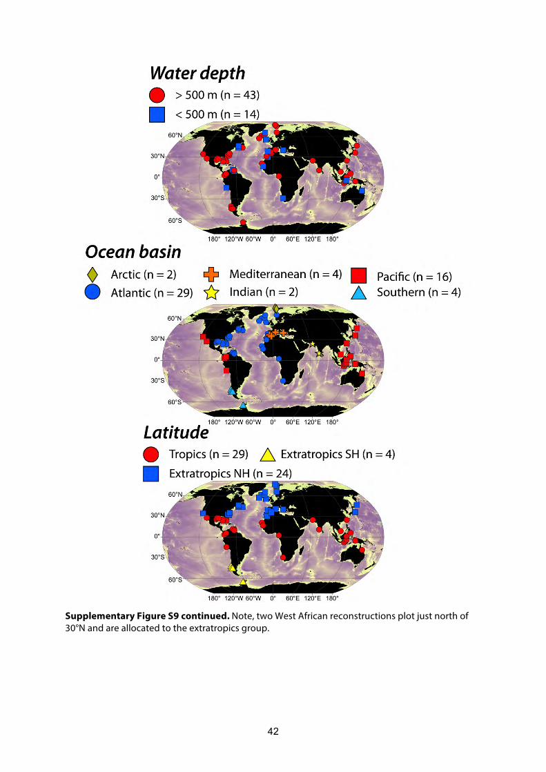
42

Supplementary Figure S9 continued. Note, two West African reconstructions plot just north of 30°N and are allocated to the extratropics group.

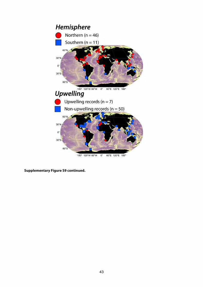
43

Supplementary Figure S9 continued.

44

Section 7: Calculation of bin-to-bin changes

We estimated the bin-to-bin change in standardized temperature (dT) as the median of all possible 2-point slopes calculable from the available values in the nth and (n-1)th bins (Supplementary Table S13). The Wilcoxon signed rank test was used to test the null hypothesis that the median slope dT was equal to zero, and the z-statistic approximation for large sample sizes was used (Davis, 2002).

Supplementary Table S13. Bin-mean standardized SST and bin-to-bin SST changes.

100 0.78 2.24 29 0.03 n/a n/a n/a n/a 300 0.58 2.35 33 0.02 -0.03 -2.51 957 0.01 500 0.39 2.24 38 0.03 -0.07 -3.58 1254 0.0003 700 0.38 2.61 43 0.01 -0.01 -1.79 1634 0.07 900 0.23 2.99 45 0.003 -0.04 -1.56 1935 0.11 1100 0.07 1.24 45 0.22 -0.07 -5.34 2025 <0.00001 1300 -0.19 -2.02 49 0.04 -0.17 -14.80 2205 <0.00001 1500 -0.70 -4.00 44 <0.0001 -0.18 -14.54 2156 <0.00001 1700 -0.71 -3.90 44 <0.0001 -0.06 -3.84 1936 0.0001 1900 -0.60 -1.64 40 0.10 0.08 5.61 1760 <0.00001

Bin center Tbin z(T) N(Tbin ) p(zT) dT z(dT) N(dT) p(zdT)(CE) (sd units) (sd units/100y)

Bin centers correspond to values dating to 1-200, 201-400, ... 1801-2000 CE.

Tbin is the median of all standardized data within the bin.

z(T) is the Wilcoxon signed rank test, z-statistic (large sample approximation) for the null hypothesis that the median standardized T within the bin is equal to zero, with the subsequent two columns the number of T_bin estimates (N(T)) and the p-value (p(zT)) that the null hypothesis is true, respectively.

dT is the median bin-to-bin change in standard deviation units per 100 years. For example, dT in the 300 bin center row is the change between the bin centered on 100 CE and the bin centered on 300 CE (see also Supplementary Methods).

z(dT) is the Wilcoxon signed rank test, z-statistic (large sample approximation) for the null hypothesis that the median dT is equal to zero, with the subsequent two columns the number of slope estimates (N(dT)), and the p-value (p(zdT)) that the null hypothesis is true, respectively.

45

Section 8: 20th century SST trends

A subset (n = 21) of the Ocean2k 57 input reconstructions are dated by 210Pb dating or annual band counting, and are of sufficient resolution to potentially record 20th century SST changes (Supplementary Table S1, column ‘High resolution reconstructions’; Supplementary Fig. S1). These reconstructions were composited into 25-year bins, beginning at 2000 CE and extending back to 1851 CE (e.g. 1851–1875 CE, 1876–1900 CE… 1976–2000 CE; Supplementary Fig. S10), by first averaging each reconstruction into one value per 25-year bin, then standardizing the reconstructions, and finally compositing the standardized reconstructions. Reconstructions were binned at 25-year resolution to account for the maximum time interval between any two samples in any individual reconstruction.

The results for the composite of the 21 highest resolution reconstructions (21_O2k) were compared to Kaplan SST reanalysis data (Kaplan et al., 1998), where the Kaplan data were extracted for the same time intervals and locations, and composited in the same way as the n = 21 Ocean2k reconstructions described above (21_Kaplan). The 21_O2k and 21_Kaplan composites are non-significantly correlated (r2 = 0.17, df = 4, p = 0.42), with the warming trend in the 21_Kaplan not reproduced in the 21_O2k composite (Supplementary Fig. S10).

Investigating further, correlation with Kaplan et al., (1998) is significant for the SST reconstructions from the tropics (n = 11; r2 = 0.67, df = 4, p = 0.05), but non-significant for non-upwelling regions (n = 14; r2 = 0.49, df = 4, p = 0.12; Supplementary Fig. S10). Non-significant correlations were also found for the Northern Hemisphere extratropics (n = 10; r2 = 0.37, df = 4, p = 0.20), upwelling regions (n = 7; r2 = 0.43, df = 4, p = 0.15), and for reconstructions based on Mg/Ca-based reconstructions (n = 4; r2 = 0.33, df = 4, p = 0.24) or alkenones (n = 15; r2 = 0.19, df = 4, p = 0.38; Supplementary Fig. S10). Note that one of the 21 reconstructions is based on coral Sr/Ca, and another is based on dinocyst assemblages. Also note that there were not sufficient reconstructions for other permutations to be tested.

Because of the limited number of composited data series within these comparisons, the limited degrees of freedom in the correlations, and the complexities of localized conditions on decadal time scales, these results suggest that these comparisons should be interpreted cautiously. For instance, in addition to uncertainties with the paleoclimate reconstructions, the cooling trend observed in the upwelling-reconstructions from eastern boundary current regions may reflect increases in land-sea temperature differences that strengthen upwelling-inducing winds (Bakun, 1990; McGregor et al., 2007; Bakun et al., 2010; Leduc et al., 2010a; Sydeman et al., 2014), that are not well captured by instrumental datasets (Falvey and Garreaud, 2009; Kennedy, 2014). In a second example, the apparent opposite sign for trends between alkenone and Mg/Ca reconstructions (Supplementary Fig. S10) may not necessarily arise from proxy differences per se (Laepple and Huybers, 2013). When we separate the alkenone reconstructions (n = 15) into upwelling and non-upwelling regions (n = 7 and n = 8, respectively; note that the upwelling group is comprised entirely of alkenone reconstructions), we observe that the non-upwelling alkenone group exhibits a direct, though non-significant correlation with Kaplan (n = 8; r2 = 0.24, df = 4, p = 0.33), in essence

46

consistent with the Mg/Ca reconstructions (Supplementary Fig. S10). Thus the apparent difference between the Mg/Ca and alkenone composites may simply reflect trends in non-upwelling versus upwelling a priori defined regions.

For the pre-industrial interval, however, where we have additional reconstructions, the decadal, seasonal and local effects are apparently averaged away on the bicentennial time scales, such that when the mean climatological SST and core-top SST reconstructions for 41 sites with data in the 1801–2000 CE interval are regressed, the regression has an intercept and slope indistinguishable, within error, from zero and one, respectively (Supplementary Discussion; Supplementary Fig. S6a).

Additional precisely-dated, high resolution and multiple-proxy records of mixed layer and atmospheric conditions are needed to better understand whether the different trends in the high-resolution subgroups are due to location, data type, or other uncertainties in the SST reconstructions. For example, six sediment core-based SST reconstructions were dated by radiocarbon and reported modern core-top ages; if these six cores were to be dated by 210Pb, and if new reconstructions from other high-sedimentation rate regions were produced, we would have a larger composite to analyze. However, even high-resolution marine sediments are a crude means by which to study historical and decadal resolution SST variation. Further analysis should focus on annually-resolved marine paleoclimate archives (e.g. corals; Tierney et al., 2015) and historical data analysis (e.g. Allan et al., 2011).

47

Supplementary Figure S10. Analysis of post-industrial SST trends. The 21 Ocean2k SST reconstructions with annual band counting or 210Pb dating (Supplementary Table S1). a. Composite (21_Kaplan) of 25-year bin Kaplan SST (Kaplan et al., 1998), where the Kaplan data were selected for the same intervals, locations as the 21 post-industrial Ocean2k SST reconstructions (21_O2k). Boxplots show 25th to 75th percentile range (box), median (black line), and outliers (crosses) to approximately 99.3% of data range (black lines) assuming bin contents are normally distributed (Methods). The mean of the

1863 1888 1913 1938 1963 1988

0

10

20

30

-2

0

2

-2

0

2

1863 1888 1913 1938 1963 1988

0

10

20

30

-2

0

2

-2

0

2

1863 1888 1913 1938 1963 1988

0

10

20

30

-2

0

2

-2

0

2

1863 1888 1913 1938 1963 1988

-2

0

2

0

10

20

30

-2

0

2

-2

0

2

-2

0

2

c

a

Year (CE)

Sta

ndar

dize

d an

omal

y(s

.d.u

nits

) S

ST

(ºC

)

Kaplan SST composite

b

d

i

j

O2k post-industrial composite

Sta

ndar

dize

d an

omal

y(s

.d.u

nits

) S

tand

ardi

zed

anom

aly

(s.d

.uni

ts)

Sta

ndar

dize

d an

omal

y(s

.d.u

nits

)

Non-upwelling composite

Upwelling composite

Year (CE) S

ST

(ºC

)

e

k

l

Sta

ndar

dize

d an

omal

y(s

.d.u

nits

) S

tand

ardi

zed

anom

aly

(s.d

.uni

ts)

Mg/Ca composite

Alkenone composite

Year (CE)

SS

T (º

C)

g

h

Sta

ndar

dize

d an

omal

y(s

.d.u

nits

) S

tand

ardi

zed

anom

aly

(s.d

.uni

ts)

Tropical composite

Extra-tropical NH composite

Non-upwelling versus UpwellingTropical versus Extra-tropical NH Mg/Ca versus AlkenonesAlkenones only

Non-upwelling versus Upwelling

SS

T (º

C)

f

m

n

Sta

ndar

dize

d an

omal

y(s

.d.u

nits

) S

tand

ardi

zed

anom

aly

(s.d

.uni

ts)

Upwelling composite

Non-upwelling composite

Year (CE)

Mg/Ca

48

composite is also shown (black line and yellow circles). b. As for a) except using the 21 post-industrial Ocean2k SST reconstructions. c. Raw data series of n = 11 post-industrial Ocean2k SST reconstructions from the tropics (red lines) and n = 10 reconstructions from the Northern Hemisphere extratropics (blue lines). d. n = 14 reconstructions from non-upwelling regions (red lines) and n = 7 reconstructions from upwelling regions (blue lines), as defined in the Supplementary Section 1 and Supplementary Table S3. e. n=4 reconstructions based on foraminifera Mg/Ca (red lines) and n=15 reconstructions based on alkenones (blue lines). f. n=8 reconstructions based on alkenones and from non-upwelling regions (red lines) and n=7 reconstructions based on alkenones and from upwelling regions (blue lines). g,h. As for b) except using only the reconstructions from the tropics and Northern Hemisphere extratropics highlighted in c). i.j. As for b) except using only the reconstructions from the non-upwelling and upwelling highlighted in d). k,l. As for b) except using only the reconstructions from foraminifera Mg/Ca and alkenones highlighted in e). m,n. As for b) except using only the reconstructions from alkenones in non-upwelling regions and alkenones in upwelling regions highlighted in f)).

49

Section 9: Paleoclimate data and model simulation comparison

Method for constructing the Terrestrial 2k composite

The Terrestrial 2k composite for 801–1800 CE (to match the model simulations) uses a non-marine subset of proxy observations from the PAGES 2k Consortium (2013; their Supplemental Table S2, and also available from https://www.ncdc.noaa.gov/cdo/f?p=519:2:0::::P1_study_id:12621), and with updates from McKay and Kaufman (2014; update 1.1.1 from http://dx.doi.org/10.6084/m9.figshare.1054736). Excluded data series are 1) Australian series: 3, 12, 14, 16–19, 21–24, 27–28 (coral), 2) Arctic series: 38, 39, 47, 55, 57, 58 (sediment core proxies), and 3) South American series: 4 (sediment core Mg/Ca). As per the PAGES 2k Consortium (2013) synthesis no Africa reconstructions are included. The number of observations per 200-year bin ranges from 48 to 316 (Supplementary Table S13). The Terrestrial 2k composite was binned and composited as per the Ocean2k synthesis.

50

Supplementary Table S14: Paleoclimate data and model simulation trend statistics

Supplementary Table S14. Statistics of cooling trend estimates for each composite shown in Figure 3, Figure 4 and Supplementary Figure S11.

p m N 801-1000 CE# 1001-1200 CE 1201-1400 CE 1401-1600 CE 1601-1800 CE

Ocean2k SST synthesis (801-1800 CE) 0.82 -1.49 44 45 49 44 40

Terrestrial2k composite 0.73 -0.81 70 183 207 258 338

Multi-model composite 0.91 -1.85 264 270 293* 262* 238*

CSIRO Mk3L model simulations (cumulative addition of forcings)

Orbital 0.53 -0.13 44 45 49 44 40

Orbital + Greenhouse Gas 0.60 -0.30 44 45 49 44 40

Orbital + Greenhouse Gas + Solar 0.67 -0.62 44 45 49 44 40

Orbital + Greenhouse Gas + Solar + Volcanic 0.95 -2.08 44 45 49 44 40

LOVECLIM model simulations (individual forcings)

Orbital 0.56 -0.22 44 45 49 44 40

Greenhouse Gas 0.55 -0.18 44 45 49 44 40

Solar 0.49 0.02 44 45 49 44 40

Volcanic 0.71 -0.70 44 45 49 44 40

Land Use 0.79 -1.12 44 45 49 44 40

All forcings 0.93 -1.71 44 45 49 44 40

p = probability that the temporal trend is negative from each preceding bin.m = slope of the linear regression in standard deviation units / ka.N = number of reconstructions contributing to each bin* N for the multi-model composite (six model simulations) should be six times larger than N(Ocean2k). This is not the case for the bins centered on 1700, 1500, and 1300 CE. This is because at the location masked for the availability of data from Pahnke et al. (2007), the bcc-csm-1 bin means for 1401-1600 CE and 1601-1800 CE are identical and therefore standardizing to unit variance results in NaN. This also occurs at the location masked for the availability of data from Newton et al. (2011) for the bins centered on 1300, 1500, and 1700 CE.As an example, in the bin centered on 1700 CE, there are !ve model simulations with values at 40 locations (the same as N(Ocean2k)), and one model (bcc-cam-1) with values at only 38 locations, giving a total of N(model) = 238. # Model simulations for BCC-CSM1-1, CCSM4, FGOALS-s2, LOVECLIM, MPI-ESM end at 850 CE.

51

Supplementary Figure S11: Single and cumulative forcing simulation plots

Supplementary Figure S11 shows the 801-1800 CE trends and slope estimates for each CSIRO Mk3L cumulative forcing simulation, and for each LOVECLIM single forcing simulation. The slopes and negative slope probabilities are presented in Figure 4, with the trend statistics given in Supplementary Table S14 (and in Supplementary Tables S8-S9). See Methods and Supplementary Section 2 for model simulation details.

Supplementary Figure S11. Cumulative forcing CSIRO Mk3L and single forcing LOVECLIM model simulation trends for 801–1800 CE. Boxplots show 25th to 75th percentile range (blue box), median (red line), and outliers (red crosses) to approximately 99.3% of data range (blue ‘whiskers’) assuming bin contents are Gaussian distributed (Methods). Distribution (grey lines) and median (black line) of 10,000 Monte-Carlo trend estimates are displayed for each synthesis. Supplementary Tables S14, and S8–S9 gives the trend statistics.

52

Section 10: Energy Balance Model methods

The Energy Balance Model (EBM) applied in Figure 4 is based on a very simple equation for the global mean surface temperature TS (e.g. Watterson, 2000):

Ss f Sd TC Q Tdt

λΔ

= Δ + Δ

where the left-hand side represents the changes in heat content of the climate system and the right hand side the radiative balance at the top of the atmosphere. ΔQ is the radiative forcing, here taken as the volcanic forcing from Crowley (2008), λf is the climate feedback parameter (λf = -1.23 W m-2 K-1 , corresponding to a climate sensitivity of 3°C). Cs is the heat capacity of the system, taken equal to the one of an oceanic mixed layer of a 200m thickness (Cs =8.36 108 J K-1 m-2; for more details, see for instance Goosse et al., (2015), http://www.climate.be/textbook/chapter4_node5.xml).

53

Section 11: Volcanic forcing and LOVECLIM and CSIRO Mk3L model simulations

We test for persistent impacts of volcanic clusters on the strength of the Atlantic Meridional Overturning Circulation (AMOC) by (a) examining the volcanic-only forcing LOVECLIM simulation, and (b) comparing the orbital-greenhouse gas-solar (OGS) and orbital-greenhouse gas-solar-volcanic (OGSV) forcing CSIRO Mk3L simulations (Supplementary Figs. S12 and S13). In neither model do we find a persistent weakening of the AMOC in response to clusters of volcanic eruptions over the past millennium. Rather, we find a tendency towards a stronger AMOC and enhanced Northern Hemisphere sea ice volume during the years immediately following major eruptions. These responses are transient in nature and do not persist.

Supplementary Figure S12. Annual-mean volcanic radiative forcing, and LOVECLIM model simulation of Northern Hemisphere (NH) sea ice volume and Atlantic Meridional Overturning Circulation (AMOC) strength for 850-1850 CE. Results of LOVECLIM model simulations with volcanic forcing only, in grey for the ensemble members and in black for the ensemble mean. Note for the sea ice volume only mean annual data were available.

54

Supplementary Figure S13. Annual-mean volcanic radiative forcing, and CSIRO Mk3L model simulation of NH sea ice volume in September, and AMOC strength for 850–1850 CE. CSIRO Mk3L orbital-greenhouse gas-solar forcing (OGS) results for the average (thick black line) of three ensemble members (thin black line) and orbital-greenhouse gas-solar-volcanic (OGSV) forcing results for the average (thick red line) of three ensemble members (thin red line). Model results are plotted as a 30-year running mean.

55

Section 12: Supplementary References

Abrantes, F., Lebreiro, S., Rodrigues, T., Gila, I., Bartels-Jónsdóttir, H., Oliveira, P., Kissel, C., Grimalt, J.O. (2005) Shallow-marine sediment cores record climate variability and earthquake activity off Lisbon (Portugal) for the last 2000 years. Quaternary Science Reviews, 24:2477-2494.

Alibert, C., McCulloch, M.T. (1997) Strontium/calcium ratios in modern Porites corals from the Great Barrier Reef as a proxy for sea surface temperature: Calibration of the thermometer and monitoring of ENSO. Paleoceanography, 12:345-363, 10.1029/97PA00318.

Allan, R., Brohan, P., Compo, G.P., Stone, R., Luterbacher, J., Bronniman, S. (2011) The International Atmospheric Circulation Reconstructions over the Earth (ACRE) Initiative. Bulletin of the American Meteorological Society, 92:1421-1425, 10.1175/2011BAMS3218.1.

Anand, P., Elderfield, H., Conte, M.H. (2003) Calibration of Mg/Ca thermometry in planktonic foraminifera from a sediment trap time series. Paleoceanography, 18:1050, 10.1029/2002pa000846.

Andresen, C.S., Hansen, M.J., Seidenkrantz, M.-S., Jennings, A.E., Knudsen, M.F., Nørgaard-Pedersen, N., Larsen, N.K., Kuijpers, A., Pearce, C. (2013) Mid- to late-Holocene oceanographic variability on the Southeast Greenland shelf. The Holocene, 23:167-178, 10.1177/0959683612460789.

Andruleit, H., Stäger, S., Rogalla, U., Čepek, P. (2003) Living coccolithophores in the northern Arabian Sea: ecological tolerances and environmental control. Marine Micropaleontology, 49:157-181, 10.1016/S0377-8398(03)00049-5.

Arbuszewski, J., deMenocal, P., Kaplan, A., Farmer, E.C. (2010) On the fidelity of shell-derived δ18Oseawater estimates. Earth and Planetary Science Letters, 300:185-196, 10.1016/j.epsl.2010.10.035.

Bakun, A. (1990) Global climate change and intensification of coastal ocean upwelling. Science, 247:198-201, 10.1126/science.247.4939.198.

Bakun, A., Field, D.B., Redondo-Rodriguez, A., Weeks, S.J. (2010) Greenhouse gas, upwelling-favorable winds, and the future of coastal ocean upwelling ecosystems. Global Change Biology, 16:1213-1228, 10.1111/j.1365-2486.2009.02094.x.

Bard, E., Arnold, M., Fairbanks, R.G., Hamelin, B. (1993) 230Th-234U and 14C ages obtained by mass spectrometery on corals. Raidocarbon, 35:191-199.

Barker, S., Cacho, I., Benway, H., Tachikawa, K. (2005) Planktonic foraminiferal Mg/Ca as a proxy for past oceanic temperatures: a methodological overview and data compilation for the Last Glacial Maximum. Quaternary Science Reviews, 24:821-834, 10.1016/j.quascirev.2004.07.016.

Barker, S., Greaves, M., Elderfield, H. (2003) A study of cleaning procedures used for foraminiferal Mg/Ca paleothermometry. Geochemistry, Geophysics, Geosystems, 4:8407, 10.1029/2003gc000559.

Bé, A.W.H. (1977) An ecological zoogeographical and taxonomic review of recent planktonic foraminifera. Ramsay. A.T.S. (Ed.): Oceanic Micropaleontology. Academic Press 1, London, p. 100.

Bender, M.L., Lorens, R.B., Williams, D.F. (1975) Sodium, magnesium and strontium in the tests of planktonic foraminifera. Micropaleontology, 21:448-459.

Berger, A.L. (1978) Long-Term Variations of Daily Insolation and Quaternary Climatic Changes. Journal of the Atmospheric Sciences, 35:2362-2367, 10.1175/1520-0469(1978)035<2362:LTVODI>2.0.CO;2.

Berner, K.S., Koç, N., Godtliebsen, F., Divine, D. (2011) Holocene climate variability of the Norwegian Atlantic Current during high and low solar insolation forcing. Paleoceanography, 26:PA2220, 10.1029/2010pa002002.

56

Bijma, J., Altabet, M., Conte, M., Kinkel, H., Versteegh, G.J.M., Volkman, J.K., Wakeham, S.G., Weaver, P.P. (2001) Primary signal: Ecological and environmental factors - Report from Working Group 2. Geochemistry, Geophysics, Geosystems, 2, 10.1029/2000gc000051.

Black, D.E., Abahazi, M.A., Thunell, R.C., Kaplan, A., Tappa, E.J., Peterson, L.C. (2007) An 8-century tropical Atlantic SST record from the Cariaco Basin: Baseline variability, twentieth-century warming, and Atlantic hurricane frequency. Paleoceanography, 22:PA4204, 10.1029/2007pa001427.

Bonnet, S., de Vernal, A., Hillaire-Marcel, C., Radi, T., Husum, K. (2010) Variability of sea-surface temperature and sea-ice cover in the Fram Strait over the last two millennia. Marine Micropaleontology, 74:59-74, 10.1016/j.marmicro.2009.12.001.

Calvo, E., Grimalt, J.O., Jansen, E. (2002) High resolution U37K sea surface temperature

reconstruction in the Norwegian Sea during the Holocene. Quaternary Science Reviews, 21:1385-1394, 10.1016/S0277-3791(01)00096-8.

Came, R.E., Oppo, D.W., McManus, J.F. (2007) Amplitude and timing of temperature and salinity variability in the subpolar North Atlantic over the past 10 k.y. Geology, 35:315-318, 10.1130/g23455a.1.

Cléroux, C., Debret, M., Cortijo, E., Duplessy, J.-C., Dewilde, F., Reijmer, J., Massei, N. (2012) High-resolution sea surface reconstructions off Cape Hatteras over the last 10 ka. Paleoceanography, 27:PA1205, 10.1029/2011pa002184.

Cohen, A.L., Hart, S.R. (2004) Deglacial sea surface temperatures of the western tropical Pacific: A new look at old coral. Paleoceanography, 19:PA4031, 10.1029/2004PA001084.

Cohen, A.L., Layne, G.D., Hart, S.R., Lobel, P.S. (2001) Kinetic control of skeletal Sr/Ca in a symbiotic coral: Implications for the paleotemperature proxy. Paleoceanography, 16:20-26, 10.1029/1999pa000478.

Conte, M.H., Sicre, M.-A., Rühlemann, C., Weber, J.C., Schulte, S., Schulz-Bull, D., Blanz, T. (2006) Global temperature calibration of the alkenone unsaturation index (UK'

37) in surface waters and comparison with surface sediments. Geochemistry, Geophysics, Geosystems, 7:Q02005, 10.1029/2005gc001054.

Corrège, T. (2006) Sea surface temperature and salinity reconstruction from coral geochemical tracers. Palaeogeography, Palaeoclimatology, Palaeoecology, 232:408-428, 10.1016/j.palaeo.2005.10.014.

Crespin, E., Goosse, H., Fichefet, T., Mairesse, A., Sallaz-Damaz, Y. (2013) Arctic climate over the past millennium: Annual and seasonal responses to external forcings. The Holocene, 23:321-329, 10.1177/0959683612463095.

Crowley, T., Zielinski, G. A., Vinther, B., Udisti, R., Kreutz, K., Cole-Dai, J., Castellano, E. (2008) Volcanism and the Little Ice Age. PAGES News, 16:22-23.

Curry, W.B., Ostermann, D.R., Guptha, M.V.S., Ittekkot, V. (1992) Foraminiferal production and monsoonal upwelling in the Arabian Sea: evidence from sediment traps. Geological Society, London, Special Publications, 64:93-106, 10.1144/gsl.sp.1992.064.01.06.

Davis, J.C. (2002) Statistics and Data Analysis in Geology, 3rd ed. John Wiley and Sons, New York.

de Vernal, A., Henry, M., Matthiessen, J., Mudie, P.J., Rochon, A., Boessenkool, K.P., Eynaud, F., GrØsfjeld, K., Guiot, J., Hamel, D., Harland, R., Head, M.J., Kunz-Pirrung, M., Levac, E., Loucheur, V., Peyron, O., Pospelova, V., Radi, T., Turon, J.-L., Voronina, E. (2001) Dinoflagellate cyst assemblages as tracers of sea-surface conditions in the northern North Atlantic, Arctic and sub-Arctic seas: the new ‘n = 677’ data base and its application for quantitative palaeoceanographic reconstruction. Journal of Quaternary Science, 16:681-698, 10.1002/jqs.659.

de Vernal, A., Hillaire-Marcel, C., Rochon, A., Fréchette, B., Henry, M., Solignac, S., Bonnet, S. (2013) Dinocyst-based reconstructions of sea ice cover concentration during the Holocene in the Arctic Ocean, the northern North Atlantic Ocean and its adjacent seas. Quaternary Science Reviews, 79:111-121, 10.1016/j.quascirev.2013.07.006.

57

de Vernal, A., Hillaire-Marcel, C., Solignac, S., Radi, T., Rochon, A. (2008) Reconstructing sea ice conditions in the Arctic and sub-Arctic prior to human observations, Arctic Sea Ice Decline: Observations, Projections, Mechanisms, and Implications. AGU, Washington, DC, pp. 27-45, 10.1029/1180gm1004.

de Villiers, S., Shen, G.T., Nelson, B.K. (1994) The Sr/Ca-temperature relationship in coralline aragonite: Influence of variability in (Sr/Ca)seawater and skeletal growth parameters. Geochimica et Cosmochimica Acta, 58:197-208, 10.1016/0016-7037(94)90457-X.

Dekens, P.S., Lea, D.W., Pak, D.K., Spero, H.J. (2002) Core top calibration of Mg/Ca in tropical foraminifera: Refining paleotemperature estimation. Geochemistry, Geophysics, Geosystems, 3:1-29, 10.1029/2001gc000200.

Delaygue, G., Bard, E. (2011) An Antarctic view of Beryllium-10 and solar activity for the past millennium. Climate Dynamics, 36:2201-2218, 10.1007/s00382-010-0795-1.

deMenocal, P., Ortiz, J., Guilderson, T., Sarnthein, M. (2000) Coherent high- and low-latitude climate variability during the Holocene warm period. Science, 288:2198-2202, 10.1126/science.288.5474.2198.

Deuser, W.G. (1987) Seasonal variations in isotopic composition and deep-water fluxes of the tests of perennially abundant planktonic foraminifera of the Sargasso Sea; results from sediment-trap collections and their paleoceanographic significance. The Journal of Foraminiferal Research, 17:14-27, 10.2113/gsjfr.17.1.14.

Dolven, J.K., Cortese, G., Bjørklund, K.R. (2002) A high-resolution radiolarian-derived paleotemperature record for the Late Pleistocene-Holocene in the Norwegian Sea. Paleoceanography, 17:1072, 10.1029/2002pa000780.

Doose-Rolinski, H., Rogalla, U.R., Scheeder, G., Lückge, A., von Rad, U. (2001) High-resolution temperature and evaporation changes during the late Holocene in the northeastern Arabian Sea. Paleoceanography, 16:358-367, 10.1029/2000pa000511.

Eguchi, N.O., Ujiié, H., Kawahata, H., Taira, A. (2003) Seasonal variations in planktonic foraminifera at three sediment traps in the Subarctic, Transition and Subtropical zones of the central North Pacific Ocean. Marine Micropaleontology, 48:149-163, 10.1016/S0377-8398(03)00020-3.

Enmar, R., Stein, M., Bar-Matthews, M., Sass, E., Katz, A., Lazar, B. (2000) Diagenesis in live corals from the Gulf of Aqaba. I. The effect on paleo-oceanography tracers. Geochimica et Cosmochimica Acta, 64:3123-3132, 10.1016/S0016-7037(00)00417-8.

Falvey, M., Garreaud, R.D. (2009) Regional cooling in a warming world: Recent temperature trends in the southeast Pacific and along the west coast of subtropical South America (1979–2006). Journal of Geophysical Research, 114:D04102, 10.1029/2008JD010519.

Gaetani, G.A., Cohen, A.L., Wang, Z.R., Crusius, J. (2011) Rayleigh-based, multi-element coral thermometry: A biomineralization approach to developing climate proxies. Geochimica et Cosmochimica Acta, 75:1920-1932, 10.1016/j.gca.2011.01.010.

Gagan, M.K., Dunbar, G.B., Suzuki, A. (2012) The effect of skeletal mass accumulation in Porites on coral Sr/Ca and δ18O paleothermometry. Paleoceanography, 27:PA1203, 10.1029/2011pa002215.

Gao, C., Robock, A., Ammann, C. (2008) Volcanic forcing of climate over the past 1500 years: An improved ice core-based index for climate models. Journal of Geophysical Research, 113:D23111, 10.1029/2008jd010239.

Goni, M.A., Thunell, R.C., Woodwort, M.P., Müller-Karger, F.E. (2006) Changes in wind-driven upwelling during the last three centuries: Interocean teleconnections. Geophysical Research Letters, 33:L15604, 10.1029/2006gl026415.

Goosse, H., Barriat, P.Y., Lefebvre, W., Loutre, M.F., Zunz, V. (2015) Introduction to climate dynamics and climate modeling. Online textbook available at http://www.climate.be/textbook.

Goosse, H., Brovkin, V., Fichefet, T., Haarsma, R., Huybrechts, P., Jongma, J., Mouchet, A., Selten, F., Barriat, P.Y., Campin, J.M., Deleersnijder, E., Driesschaert, E., Goelzer, H., Janssens, I., Loutre, M.F., Morales Maqueda, M.A., Opsteegh, T., Mathieu, P.P., Munhoven, G., Pettersson, E.J., Renssen, H., Roche, D.M., Schaeffer, M., Tartinville,

58

B., Timmermann, A., Weber, S.L. (2010) Description of the Earth system model of intermediate complexity LOVECLIM version 1.2. Geosci. Model Dev., 3:603-633, 10.5194/gmd-3-603-2010.

Grauel, A.-L., Leider, A., Goudeau, M.-L.S., Müller, I.A., Bernasconi, S.M., Hinrichs, K.-U., de Lange, G.J., Zonneveld, K.A.F., Versteegh, G.J.M. (2013) What do SST proxies really tell us? A high-resolution multiproxy (UK′

37, TEXH86 and foraminifera δ18O) study in the

Gulf of Taranto, central Mediterranean Sea. Quaternary Science Reviews, 73:115-131, http://dx.doi.org/10.1016/j.quascirev.2013.05.007.

Guiot, J. (1990) Methodology of the last climatic cycle reconstruction in France from pollen data. Palaeogeography, Palaeoclimatology, Palaeoecology, 80:49-69, 10.1016/0031-0182(90)90033-4.

Gutiérrez, D., Bouloubassi, I., Sifeddine, A., Purca, S., Goubanova, K., Graco, M., Field, D., Méjanelle, L., Velazco, F., Lorre, A., Salvatteci, R., Quispe, D., Vargas, G., Dewitte, B., Ortlieb, L. (2011) Coastal cooling and increased productivity in the main upwelling zone off Peru since the mid-twentieth century. Geophysical Research Letters, 38:L07603, 10.1029/2010gl046324.

Harada, N., Ahagon, N., Uchida, M., Murayama, M. (2004) Northward and southward migrations of frontal zones during the past 40 kyr in the Kuroshio-Oyashio transition area. Geochemistry, Geophysics, Geosystems, 5:Q09004, 10.1029/2004gc000740.

Hathorne, E.C., Felis, T., James, R.H., Thomas, A. (2011) Laser ablation ICP-MS screening of corals for diagenetically affected areas applied to Tahiti corals from the last deglaciation. Geochimica et Cosmochimica Acta, 75:1490-1506, 10.1016/j.gca.2010.12.011.

Hathorne, E.C., Gagnon, A., Felis, T., Adkins, J., Asami, R., Boer, W., Caillon, N., Case, D., Cobb, K.M., Douville, E., deMenocal, P., Eisenhauer, A., Garbe-Schönberg, D., Geibert, W., Goldstein, S., Hughen, K., Inoue, M., Kawahata, H., Kölling, M., Cornec, F.L., Linsley, B.K., McGregor, H.V., Montagna, P., Nurhati, I.S., Quinn, T.M., Raddatz, J., Rebaubier, H., Robinson, L., Sadekov, A., Sherrell, R., Sinclair, D., Tudhope, A.W., Wei, G., Wong, H., Wu, H.C., You, C.-F. (2013) Interlaboratory study for coral Sr/Ca and other element/Ca ratio measurements. Geochemistry, Geophysics, Geosystems, 14:3730-3750, 10.1002/ggge.20230.

Hemleben, C., Spindler, M., Anderson, O.R. (1989) Modern Planktonic Foraminifera. Springer New York.

Hendy, E.J., Gagan, M.K., Alibert, C.A., McCulloch, M.T., Lough, J.M., Isdale, P.J. (2002) Abrupt Decrease in Tropical Pacific Sea Surface Salinity at End of Little Ice Age. Science, 295:1511-1514, 10.1126/science.1067693.

Hendy, E.J., Gagan, M.K., Lough, J.M., McCulloch, M., deMenocal, P.B. (2007) Impact of skeletal dissolution and secondary aragonite on trace element and isotopic climate proxies in Porites corals. Paleoceanography, 22:PA4101, 10.1029/2007pa001462.

Hendy, I.L., Dunn, L., Schimmelmann, A., Pak, D.K. (2012) Resolving varve and radiocarbon chronology differences during the last 2000 years in the Santa Barbara Basin sedimentary record, California. Quaternary International, 310:155-168, 10.1016/j.quaint.2012.09.006.

Hönisch, B., Allen, K.A., Lea, D.W., Spero, H.J., Eggins, S.M., Arbuszewski, J., deMenocal, P., Rosenthal, Y., Russell, A.D., Elderfield, H. (2013) The influence of salinity on Mg/Ca in planktic foraminifers – Evidence from cultures, core-top sediments and complementary δ18O. Geochimica et Cosmochimica Acta, 121:196-213, 10.1016/j.gca.2013.07.028.

Hughen, K.A., Baillie, M.G.L., Bard, E., Beck, J.W., Bertrand, C.J.H., Blackwell, P.G., Buck, C.E., Burr, G.S., Cutler, K.B., Damon, P.E., Edwards, R.L., Fairbanks, R.G., Friedrich, M., Guilderson, T.P., Kromer, B., McCormac, G., Manning, S., Ramsey, C.B., Reimer, P.J., Reimer, R.W., Remmele, S., Southon, J.R., Stuiver, M., Talamo, S., Taylor, F.W., van der Plicht, J., Weyhenmeyer, C.E. (2004) Marine04 marine radiocarbon age calibration, 0-26 cal kyr BP. Radiocarbon, 46:1059-1086.

59

Imbrie, J., Kipp, N.G. (1971) A new micropaleontological method for quantitative paleoclimatology: application to a late Pleistocene Caribbean core In: Turekian, K.K. (Ed.), The Late Cenozoic Glacial Ages. . Yale University Press, New Haven, pp. 71–181.

Isono, D., Yamamoto, M., Irino, T., Oba, T., Murayama, M., Nakamura, T., Kawahata, H. (2009) The 1500-year climate oscillation in the midlatitude North Pacific during the Holocene. Geology, 37:591-594, 10.1130/g25667a.1.

Jiang, H., Eiriksson, J., Schulz, M., Knudsen, K.-L., Seidenkrantz, M.-S. (2005) Evidence for solar forcing of sea-surface temperature on the North Icelandic Shelf during the late Holocene. Geology, 33:73-76, 10.1130/g21130.1.

Jungclaus, J.H., Fischer, N., Haak, H., Lohmann, K., Marotzke, J., Matei, D., Mikolajewicz, U., Notz, D., von Storch, J.S. (2013) Characteristics of the ocean simulations in the Max Planck Institute Ocean Model (MPIOM) the ocean component of the MPI-Earth system model. Journal of Advances in Modeling Earth Systems, 5:422-446, 10.1002/jame.20023.

Kaplan, A., Cane, M.A., Kushnir, Y., Clement, A.C., Blumenthal, M.B., Rajagopalan, B. (1998) Analyses of global sea surface temperature 1856–1991. Journal of Geophysical Research-Oceans, 103:18567-18589, 10.1029/97jc01736.

Kawahata, H., Nishimura, A., Gagan, M.K. (2002) Seasonal change in foraminiferal production in the western equatorial Pacific warm pool: evidence from sediment trap experiments. Deep Sea Research Part II: Topical Studies in Oceanography, 49:2783-2800, 10.1016/S0967-0645(02)00058-9.

Keigwin, L.D., Sachs, J.P., Rosenthal, Y. (2003) A 1600-year history of the Labrador Current off Nova Scotia. Climate Dynamics, 21:53-62, 10.1007/s00382-003-0316-6.

Keigwin, L.D., Sachs, J.P., Rosenthal, Y., Boyle, E.A. (2005) The 8200 year B.P. event in the slope water system, western subpolar North Atlantic. Paleoceanography, 20:PA2003, 10.1029/2004pa001074.

Kennedy, J.J. (2014) A review of uncertainty in in situ measurements and data sets of sea surface temperature. Reviews of Geophysics, 52:1-32, 10.1002/2013rg000434.

Kim, J.-H., Crosta, X., Willmott, V., Renssen, H., Bonnin, J., Helmke, P., Schouten, S., Sinninghe Damsté, J.S. (2012) Holocene subsurface temperature variability in the eastern Antarctic continental margin. Geophysical Research Letters, 39:L06705, 10.1029/2012gl051157.

Kim, J.-H., Meggers, H., Rimbu, N., Lohmann, G., Freudenthal, T., Müller, P.J., Schneider, R.R. (2007) Impacts of the North Atlantic gyre circulation on Holocene climate off northwest Africa. Geology, 35:387-390, 10.1130/g23251a.1.

Kim, J.-H., Schouten, S., Hopmans, E.C., Donner, B., Sinninghe Damsté, J.S. (2008) Global sediment core-top calibration of the TEX86 paleothermometer in the ocean. Geochimica et Cosmochimica Acta, 72:1154-1173, 10.1016/j.gca.2007.12.010.

Kim, J.-H., van der Meer, J., Schouten, S., Helmke, P., Willmott, V., Sangiorgi, F., Koç, N., Hopmans, E.C., Damsté, J.S.S. (2010) New indices and calibrations derived from the distribution of crenarchaeal isoprenoid tetraether lipids: Implications for past sea surface temperature reconstructions. Geochimica et Cosmochimica Acta, 74:4639-4654.

Kısakürek, B., Eisenhauer, A., Böhm, F., Garbe-Schönberg, D., Erez, J. (2008) Controls on shell Mg/Ca and Sr/Ca in cultured planktonic foraminiferan, Globigerinoides ruber (white). Earth and Planetary Science Letters, 273:260-269, 10.1016/j.epsl.2008.06.026.

Klinkhammer, G.P., Haley, B.A., Mix, A.C., Benway, H.M., Cheseby, M. (2004) Evaluation of automated flow-through time-resolved analysis of foraminifera for Mg/Ca paleothermometry. Paleoceanography, 19:PA4030, 10.1029/2004pa001050.

Krivova, N.A., Balmaceda L., Solanki S. K. (2007) Reconstruction of solar total irradiance since 1700 from the surface magnetic flux. Astronomy & Astrophysics, 467:335-346, 10.1051/0004-6361:20066725.

60

Kucera, M., Weinelt, M., Kiefer, T., Pflaumann, U., Hayes, A., Weinelt, M., Chen, M.-T., Mix, A.C., Barrows, T.T., Cortijo, E., Duprat, J., Juggins, S., Waelbroeck, C. (2005) Reconstruction of sea-surface temperatures from assemblages of planktonic foraminifera: multi-technique approach based on geographically constrained calibration data sets and its application to glacial Atlantic and Pacific Oceans. Quaternary Science Reviews, 24:951-998, 10.1016/j.quascirev.2004.07.014.

Kuhnert, H., Mulitza, S. (2011) Multidecadal variability and late medieval cooling of near-coastal sea surface temperatures in the eastern tropical North Atlantic. Paleoceanography, 26:PA4224, 10.1029/2011pa002130.

Laepple, T., Huybers, P. (2013) Reconciling discrepancies between Uk37 and Mg/Ca reconstructions of Holocene marine temperature variability. Earth and Planetary Science Letters, 375:418-429, 10.1016/j.epsl.2013.06.006.

Lamy, F., Rühlemann, C., Hebbeln, D., Wefer, G. (2002) High- and low-latitude climate control on the position of the southern Peru-Chile Current during the Holocene. Paleoceanography, 17:1028, 10.1029/2001pa000727.

Landrum, L., Otto-Bliesner, B.L., Wahl, E.R., Conley, A., Lawrence, P.J., Rosenbloom, N., Teng, H. (2013) Last Millennium Climate and Its Variability in CCSM4. Journal of Climate, 26:1085-1111, 10.1175/jcli-d-11-00326.1.

Lea, D.W., Mashiotta, T.A., Spero, H.J. (1999) Controls on magnesium and strontium uptake in planktonic foraminifera determined by live culturing. Geochimica et Cosmochimica Acta, 63:2369-2379, 10.1016/S0016-7037(99)00197-0.

Lea, D.W., Pak, D.K., Peterson, L.C., Hughen, K.A. (2003) Synchroneity of Tropical and High-Latitude Atlantic Temperatures over the Last Glacial Termination. Science, 301:1361-1364, 10.1126/science.1088470.

Leduc, G., Herbert, C.T., Blanz, T., Martinez, P., Schneider, R. (2010a) Contrasting evolution of sea surface temperature in the Benguela upwelling system under natural and anthropogenic climate forcings. Geophysical Research Letters, 37:L20705, 10.1029/2010gl044353.

Leduc, G., Schneider, R., Kim, J.H., Lohmann, G. (2010b) Holocene and Eemian sea surface temperature trends as revealed by alkenone and Mg/Ca paleothermometry. Quaternary Science Reviews, 29:989-1004.

Linsley, B.K., Rosenthal, Y., Oppo, D.W. (2010) Holocene evolution of the Indonesian throughflow and the western Pacific warm pool. Nature Geoscience, 3:578-583, 10.1038/ngeo920.

Locarnini, R.A., Mishonov, A.V., Antonov, J.I., Boyer, T.P., Garcia, H.E., Baranova, O.K., Zweng, M.M., Johnson, D.R. (2010) Volume 1: Temperature, in: Levitus, S. (Ed.), World Ocean Atlas 2009. NOAA Atlas NESDIS 68 U.S. Government Printing Office, Washington, D.C., p. 184.

Lohmann, G., Pfeiffer, M., Laepple, T., Leduc, G., Kim, J.H. (2013) A model–data comparison of the Holocene global sea surface temperature evolution. Climate of the Past, 9:1807-1839, 10.5194/cp-9-1807-2013.

Lund, D.C., Curry, W. (2006) Florida Current surface temperature and salinity variability during the last millennium. Paleoceanography, 21:PA2009, 10.1029/2005pa001218.

MacFarling Meure, C., Etheridge, D., Trudinger, C., Steele, P., Langenfelds, R., van Ommen, T., Smith, A., Elkins, J. (2006) Law Dome CO2, CH4 and N2O ice core records extended to 2000 years BP. Geophysical Research Letters, 33:L14810, 10.1029/2006gl026152.

Martínez-Botí, M.A., Mortyn, P.G., Schmidt, D.N., Vance, D., Field, D.B. (2011) Mg/Ca in foraminifera from plankton tows: Evaluation of proxy controls and comparison with core tops. Earth and Planetary Science Letters, 307:113-125, 10.1016/j.epsl.2011.04.019.

Masson-Delmotte, V., Schulz, M., Abe-Ouchi, A., Beer, J., Ganopolski, A., González Rouco, J.F., Jansen, E., Lambeck, K., Luterbacher, J., Naish, T., Osborn, T., Otto-Bliesner, B., Quinn, T., Ramesh, R., Rojas, M., Shao, X., Timmermann, A. (2013) Information from Paleoclimate Archives, in: Stocker, T.F., Qin, D., Plattner, G.-K., Tignor, M., Allen, S.K., Boschung, J., Nauels, A., Xia, Y., Bex, V., Midgley, P.M. (Eds.), Climate Change 2013:

61

The Physical Science Basis. Contribution of Working Group I to the Fifth Assessment Report of the Intergovernmental Panel on Climate Change. Cambridge University Press, Cambridge, United Kingdom and New York, NY, USA.

Mathien-Blard, E., Bassinot, F. (2009) Salinity bias on the foraminifera Mg/Ca thermometry: Correction procedure and implications for past ocean hydrographic reconstructions. Geochemistry, Geophysics, Geosystems, 10:Q12011, 10.1029/2008gc002353.

McConnaughey, T. (1989a) 13C and 18O isotopic disequilibrium in biological carbonate: II. In vitro simulation of kinetic isotope effects. Geochimica et Cosmochimica Acta, 53:163-171.

McConnaughey, T. (1989b) 13C and 18O isotopic disequilibrium in biological carbonates: I. Patterns. Geochimica et Cosmochimica Acta, 53:151-162.

McConnell, M.C., Thunell, R.C. (2005) Calibration of the planktonic foraminiferal Mg/Ca paleothermometer: Sediment trap results from the Guaymas Basin, Gulf of California. Paleoceanography, 20:PA2016, 10.1029/2004pa001077.

McGregor, H.V., Dima, M., Fischer, H.W., Mulitza, S. (2007) Rapid 20th-Century Increase in Coastal Upwelling off Northwest Africa. Science, 315:637-639, 10.1126/science.1134839.

McGregor, H.V., Gagan, M.K. (2003) Diagenesis and geochemistry of Porites corals from Papua New Guinea: Implications for paleoclimate reconstruction. Geochimica et Cosmochimica Acta, 67:2147-2156, 10.1016/S0016-7037(02)01050-5.

McKay, N.P., Kaufman, D.S. (2014) An extended Arctic proxy temperature database for the past 2,000 years. Scientific Data, 1, 10.1038/sdata.2014.26.

Menard, H.W., Smith, S.M. (1966) Hypsometry of ocean basin provinces. Journal of Geophysical Research, 71:4305-4325.

Miettinen, A., Divine, D., Koç, N., Godtliebsen, F., Hall, I.R. (2012) Multicentennial variability of the sea surface temperature gradient across the subpolar North Atlantic over the last 2.8 kyr. Journal of Climate, 10.1175/jcli-d-11-00581.1.

Mohtadi, M., Romero, O.E., Kaiser, J., Hebbeln, D. (2007) Cooling of the southern high latitudes during the Medieval Period and its effect on ENSO. Quaternary Science Reviews, 26:1055-1066, 10.1016/j.quascirev.2006.12.008.

Mohtadi, M., Steinke, S., Groeneveld, J., Fink, H.G., Rixen, T., Hebbeln, D., Donner, B., Herunadi, B. (2009) Low-latitude control on seasonal and interannual changes in planktonic foraminiferal flux and shell geochemistry off south Java: A sediment trap study. Paleoceanography, 24:PA1201, 10.1029/2008pa001636.

Mollenhauer, G., Eglinton, T.I., Ohkouchi, N., Schneider, R.R., Müller, P.J., Grootes, P.M., Rullkötter, J. (2003) Asynchronous alkenone and foraminifera records from the Benguela Upwelling System. Geochimica et Cosmochimica Acta, 67:2157-2171, 10.1016/S0016-7037(03)00168-6.

Mollenhauer, G., Kienast, M., Lamy, F., Meggers, H., Schneider, R.R., Hayes, J.M., Eglinton, T.I. (2005) An evaluation of 14C age relationships between co-occurring foraminifera, alkenones, and total organic carbon in continental margin sediments. Paleoceanography, 20:PA1016, 10.1029/2004pa001103.

Moreno, A., Pérez, A., Frigola, J., Nieto-Moreno, V., Rodrigo-Gámiz, M., Martrat, B., González-Sampériz, P., Morellón, M., Martín-Puertas, C., Corella, J.P., Belmonte, Á., Sancho, C., Cacho, I., Herrera, G., Canals, M., Grimalt, J.O., Jiménez-Espejo, F., Martínez-Ruiz, F., Vegas-Vilarrúbia, T., Valero-Garcés, B.L. (2012) The Medieval Climate Anomaly in the Iberian Peninsula reconstructed from marine and lake records. Quaternary Science Reviews, 43:16-32, 10.1016/j.quascirev.2012.04.007.

Müller, A., Gagan, M.K., McCulloch, M.T. (2001) Early marine diagenesis in corals and geochemical consequences for paleoceanographic reconstructions. Geophysical Research Letters, 28:4471-4474, 10.1029/2001gl013577.

Müller, P.J., Kirst, G., Ruhland, G., von Storch, I., Rosell-Melé, A. (1998) Calibration of the alkenone paleotemperature index U37

K' based on core-tops from the eastern South Atlantic and the global ocean (60°N-60°S). Geochimica et Cosmochimica Acta, 62:1757-1772, 10.1016/S0016-7037(98)00097-0.

62

Myhre, G., Highwood, E.J., Shine, K.P., Stordal, F. (1998) New estimates of radiative forcing due to well mixed greenhouse gases. Geophysical Research Letters, 25:2715-2718.

Newton, A., Thunell, R., Stott, L. (2011) Changes in the Indonesian Throughflow during the past 2000 yr. Geology, 39:63-66, 10.1130/g31421.1.

Nieto-Moreno, V., Martínez-Ruiz, F., Willmott, V., García-Orellana, J., Masqué, P., Sinninghe Damsté, J.S. (2013) Climate conditions in the westernmost Mediterranean over the last two millennia: An integrated biomarker approach. Organic Geochemistry, 55:1-10, 10.1016/j.orggeochem.2012.11.001.

Nürnberg, D., Bijma, J., Hemleben, C. (1996) Assessing the reliability of magnesium in foraminiferal calcite as a proxy for water mass temperatures. Geochimica et Cosmochimica Acta, 60:803-814, 10.1016/0016-7037(95)00446-7.

Ohkouchi, N., Eglinton, T.I., Keigwin, L.D., Hayes, J.M. (2002) Spatial and Temporal Offsets Between Proxy Records in a Sediment Drift. Science, 298:1224-1227, 10.1126/science.1075287.

Oppo, D.W., Rosenthal, Y., Linsley, B.K. (2009) 2,000-year-long temperature and hydrology reconstructions from the Indo-Pacific warm pool. Nature, 460:1113-1116, 10.1038/nature08233.

PAGES 2k Consortium (2013) Continental-scale temperature variability during the past two millennia. Nature Geoscience, 6:339-346, 10.1038/ngeo1797.

Pahnke, K., Sachs, J.P., Keigwin, L., Timmermann, A., Xie, S.-P. (2007) Eastern tropical Pacific hydrologic changes during the past 27,000 years from D/H ratios in alkenones. Paleoceanography, 22:PA4214, 10.1029/2007pa001468.

Pelejero, C., Grimalt, J.O. (1997) The correlation between the 37k and sea surface

temperatures in the warm boundary: The South China Sea. Geochimica et Cosmochimica Acta, 61:4789-4797, 10.1016/S0016-7037(97)00280-9.

Pflaumann, U., Sarnthein, M., Chapman, M., d'Abreu, L., Funnell, B., Huels, M., Kiefer, T., Maslin, M., Schulz, H., Swallow, J., van Kreveld, S., Vautravers, M., Vogelsang, E., Weinelt, M. (2003) Glacial North Atlantic: Sea-surface conditions reconstructed by GLAMAP 2000. Paleoceanography, 18:1065, 10.1029/2002pa000774.

Phipps, S.J., McGregor, H.V., Gergis, J., Gallant, A.J.E., Neukom, R., Stevenson, S., Ackerley, D., Brown, J.R., Fischer, M.J., van Ommen, T.D. (2013) Paleoclimate Data–Model Comparison and the Role of Climate Forcings over the Past 1500 Years. Journal of Climate, 26:6915-6936, 10.1175/jcli-d-12-00108.1.

Pongratz, J., Reick, C., Raddatz, T., Claussen, M. (2008) A reconstruction of global agricultural areas and land cover for the last millennium. Global Biogeochemical Cycles, 22:GB3018, 10.1029/2007GB003153.

Prahl, F., Herbert, T., Brassell, S.C., Ohkouchi, N., Pagani, M., Repeta, D., Rosell-Melé, A., Sikes, E. (2000) Status of alkenone paleothermometer calibration: Report from Working Group 3. Geochemistry, Geophysics, Geosystems, 1, 10.1029/2000gc000058.

Prahl, F.G., Muehlhausen, L.A., Zahnle, D.L. (1988) Further evaluation of long-chain alkenones as indicators of paleoceanographic conditions. Geochimica et Cosmochimica Acta, 52:2303-2310, 10.1016/0016-7037(88)90132-9.

Prahl, F.G., Rontani, J.-F., Zabeti, N., Walinsky, S.E., Sparrow, M.A. (2010) Systematic pattern in - Temperature residuals for surface sediments from high latitude and other oceanographic settings. Geochimica et Cosmochimica Acta, 74:131-143, 10.1016/j.gca.2009.09.027.

Prahl, F.G., Wakeham, S.G. (1987) Calibration of unsaturation patterns in long-chain ketone compositions for palaeotemperature assessment. Nature, 330:367-369, 10.1038/330367a0.

Ramankutty, N., Foley, J.A. (1999) Estimating historical changes in global land cover: Croplands from 1700 to 1992. Global Biogeochemical Cycles, 13:997-1027, 10.1029/1999GB900046.

Reimer, P.J., Baillie, M.G.L., Bard, E., Bayliss, A., Beck, J.W., Blackwell, P.G., Ramsey, C.B., Buck, C.E., Burr, G.S., Edwards, R.L., Friedrich, M., Grootes, P.M., Guilderson,

63

T.P., Hajdas, I., Heaton, T.J., Hogg, A.G., Hughen, K.A., Kaiser, K.F., Kromer, B., McCormac, F.G., Manning, S.W., Reimer, R.W., Richards, D.A., Southon, J.R., Talamo, S., Turney, C.S.M., van der Plicht, J., Weyhenmeyer, C.E. (2009) IntCal09 and Marine09 radiocarbon age calibration curves, 0-50,000 years cal BP. Raidocarbon, 51:1111-1150.

Reimer, P.J., Bard, E., Bayliss, A., Beck, J.W., Blackwell, P.G., Ramsey, C.B., Buck, C.E., Cheng, H., Edwards, R.L., Friedrich, M., Grootes, P.M., Guilderson, T.P., Haflidason, H., Hajdas, I., Heaton, T.J., Hoffmann, D.L., Hogg, A.G., Hughen, K.A., Kaiser, K.F., Kromer, B., Manning, S.W., Niu, M., Reimer, R.W., Richards, D.A., Scott, E.M., Southon, J.R., Staff, R.A., Turney, C.S.M., van der Plicht, J. (2013) IntCal13 and Marine13 radiocarbon age calibration curves 0-50,000 years cal BP. Radiocarbon, 55:1869-1887.

Richey, J.N., Poore, R.Z., Flower, B.P., Quinn, T.M. (2007) 1400 yr multiproxy record of climate variability from the northern Gulf of Mexico. Geology, 35:423-426, 10.1130/g23507a.1.

Richey, J.N., Poore, R.Z., Flower, B.P., Quinn, T.M., Hollander, D.J. (2009) Regionally coherent Little Ice Age cooling in the Atlantic Warm Pool. Geophysical Research Letters, 36:L21703, 10.1029/2009gl040445.

Richter, T.O., Peeters, F.J.C., van Weering, T.C.E. (2009) Late Holocene (0-2.4 ka BP) surface water temperature and salinity variability, Feni Drift, NE Atlantic Ocean. Quaternary Science Reviews, 28:1941-1955, 10.1016/j.quascirev.2009.04.008.

Ruddiman, W.F., Glover, L.K. (1975) Subpolar North Atlantic circulation at 9300 yr BP: Faunal evidence. Quaternary Research, 5:361-389, 10.1016/0033-5894(75)90038-1.

Rühlemann, C., Butzin, M. (2006) Alkenone temperature anomalies in the Brazil-Malvinas Confluence area caused by lateral advection of suspended particulate material. Geochemistry, Geophysics, Geosystems, 7:Q10015, 10.1029/2006gc001251.

Sachs, J.P. (2007) Cooling of Northwest Atlantic slope waters during the Holocene. Geophysical Research Letters, 34:L03609, 10.1029/2006gl028495.

Saenger, C., Came, R.E., Oppo, D.W., Keigwin, L.D., Cohen, A.L. (2011) Regional climate variability in the western subtropical North Atlantic during the past two millennia. Paleoceanography, 26:PA2206, 10.1029/2010pa002038.

Saraswat, R., Lea, D.W., Nigam, R., Mackensen, A., Naik, D.K. (2013) Deglaciation in the tropical Indian Ocean driven by interplay between the regional monsoon and global teleconnections. Earth and Planetary Science Letters, 375:166-175, 10.1016/j.epsl.2013.05.022.

Sautter, L.R., Thunell, R.C. (1991) Planktonic foraminiferal response to upwelling and seasonal hydrographic conditions; sediment trap results from San Pedro Basin, Southern California Bight. The Journal of Foraminiferal Research, 21:347-363, 10.2113/gsjfr.21.4.347.

Schimmelmann, A., Hendy, I.L., Dunn, L., Pak, D.K., Lange, C.B. (2013) Revised ∼2000-year chronostratigraphy of partially varved marine sediment in Santa Barbara Basin, California. GFF, 135:258-264, 10.1080/11035897.2013.773066.

Schneider, B., Leduc, G., Park, W. (2010) Disentangling seasonal signals in Holocene climate trends by satellite-model-proxy integration. Paleoceanography, 25:PA4217, 10.1029/2009pa001893.

Schouten, S., Hopmans, E.C., Schefuß, E., Sinninghe Damsté, J.S. (2002) Distributional variations in marine crenarchaeotal membrane lipids: a new tool for reconstructing ancient sea water temperatures? Earth and Planetary Science Letters, 204:265-274, 10.1016/S0012-821X(02)00979-2.

Seidenkrantz, M.-S. (1993) Subrecent changes in the foraminiferal distribution in the Kattegat and the Skagerrak, Scandinavia: anthropogenic influence and natural causes. Boreas, 22:383-395, 10.1111/j.1502-3885.1993.tb00201.x.

Sepúlveda, J., Pantoja, S., Hughen, K.A., Bertrand, S., Figueroa, D., León, T., Drenzek, N.J., Lange, C. (2009) Late Holocene sea-surface temperature and precipitation variability in

64

northern Patagonia, Chile (Jacaf Fjord, 44°S). Quaternary Research, 72:400-409, 10.1016/j.yqres.2009.06.010.

Shevenell, A.E., Ingalls, A.E., Domack, E.W., Kelly, C. (2011) Holocene Southern Ocean surface temperature variability west of the Antarctic Peninsula. Nature, 470:250-254, 10.1038/nature09751.

Sicre, M.-A., Hall, I.R., Mignot, J., Khodri, M., Ezat, U., Truong, M.X., Eiríksson, J., Knudsen, K.-L. (2011) Sea surface temperature variability in the subpolar Atlantic over the last two millennia. Paleoceanography, 26:PA4218, 10.1029/2011pa002169.

Sicre, M.-A., Labeyrie, L., Ezat, U., Duprat, J., Turon, J.L., Schmidt, S., Michel, E., Mazaud, A. (2005) Mid-latitude Southern Indian Ocean response to Northern Hemisphere Heinrich events. Earth and Planetary Science Letters, 240:724-731, 10.1016/j.epsl.2005.09.032.

Sicre, M.-A., Ternois, Y., Miquel, J.-C., Marty, J.-C. (1999) Alkenones in the northwestern Mediterranean Sea: Interannual variability and vertical transfer. Geophysical Research Letters, 26:1735-1738, 10.1029/1999GL900353.

Sicre, M.-A., Weckström, K., Seidenkrantz, M.-S., Kuijpers, A., Benetti, M., Masse, G., Ezat, U., Schmidt, S., Bouloubassi, I., Olsen, J., Khodri, M., Mignot, J. (2014) Labrador current variability over the last 2000 years. Earth and Planetary Science Letters, 400:26-32, 10.1016/j.epsl.2014.05.016.

Smith, S.V., Buddemeier, R.W., Redalje, R.C., Houck, J.E. (1979) Strontium-Calcium Thermometry in Coral Skeletons. Science, 204:404-407, 10.1126/science.204.4391.404.

Solignac, S., Seidenkrantz, M.-S., Jessen, C., Kuijpers, A., Gunvald, A.K., Olsen, J. (2011) Late-Holocene sea-surface conditions offshore Newfoundland based on dinoflagellate cysts. The Holocene, 21:539-552, 10.1177/0959683610385720.

Sonzogni, C., Bard, E., Rostek, F., Dollfus, D., Rosell-Melé, A., Eglinton, G. (1997) Temperature and salinity effects on alkenone ratios measured in surface sediments from the Indian Ocean. Quaternary Research, 47:344-355, 10.1006/qres.1997.1885.

Spielhagen, R.F., Werner, K., Sørensen, S.A., Zamelczyk, K., Kandiano, E., Budeus, G., Husum, K., Marchitto, T.M., Hald, M. (2011) Enhanced Modern Heat Transfer to the Arctic by Warm Atlantic Water. Science, 331:450-453, 10.1126/science.1197397.

Steinhilber, F., Beer, J., Fröhlich, C. (2009) Total solar irradiance during the Holocene. Geophysical Research Letters, 36:L19704, 10.1029/2009gl040142.

Stott, L., Timmermann, A., Thunell, R. (2007) Southern Hemisphere and Deep-Sea Warming Led Deglacial Atmospheric CO2 Rise and Tropical Warming. Science, 318:435-438, 10.1126/science.1143791.

Stuiver, M., Braziunas, T.F. (1993) Modeling atmospheric 14C influences and 14C ages of marine samples to 10,000 BC. Radiocarbon, 35:137-189.

Stuiver, M., Reimer, P.J., Bard, E., Warren Beck, J., Burr, G.S., Hughen, K.A., Kromer, B., McCormac, G., van der Plicht, J., Spurk, M. (1998) INTCAL98 radiocarbon age calibration, 24,000-0 cal BP. Radiocarbon, 40:1041-1083.

Sydeman, W.J., García-Reyes, M., Schoeman, D.S., Rykaczewski, R.R., Thompson, S.A., Black, B.A., Borgrad, S.J. (2014) Climate change and wind intensification in coastal upwelling ecosystems. Science, 77:77-80, 10.1126/science.1251635.

Tedesco, K.A., Thunell, R.C. (2003) Seasonal and interannual variations in planktonic foraminiferal flux and assemblage composition in the Cariaco Basin, Venezuela. The Journal of Foraminiferal Research, 33:192-210, 10.2113/33.3.192.

Telford, R.J., Li, C., Kucera, M. (2013) Mismatch between the depth habitat of planktonic foraminifera and the calibration depth of SST transfer functions may bias reconstructions. Climate of the Past, 9:859-870, 10.5194/cp-9-859-2013.

Ternois, Y., Sicre, M.-A., Boireau, A., Marty, J.-C., Miquel, J.-C. (1996) Production pattern of alkenones in the Mediterranean Sea. Geophysical Research Letters, 23:3171-3174, 10.1029/96gl02910.

65

Thornalley, D.J.R., Elderfield, H., McCave, I.N. (2009) Holocene oscillations in temperature and salinity of the surface subpolar North Atlantic. Nature, 457:711-714, 10.1038/nature07717.

Thunell, R.C., Curry, W.B., Honjo, S. (1983) Seasonal variation in the flux of planktonic foraminifera: time series sediment trap results from the Panama Basin. Earth and Planetary Science Letters, 64:44-55, 10.1016/0012-821X(83)90051-1.

Thurman, H.V., Trujillo, A.P. (2004) Introductory Oceanography, 10th ed. Pearson Prentice Hall.

Tierney, J.E., Abram, N.J., Anchukaitis, K.J., Evans, M.N., Giry, C., Kilbourne, K.H., Saenger, C.P., Wu, H.C., Zinke, J. (2015) Tropical sea-surface temperatures for the past four centuries reconstructed from coral archives. Paleoceanography, 10.1002/2014PA002717.

Versteegh, G.J.M., de Leeuw, J.W., Taricco, C., Romero, A. (2007) Temperature and productivity influences on U37

K' and their possible relation to solar forcing of the Mediterranean winter. Geochemistry, Geophysics, Geosystems, 8:Q09005, 10.1029/2006gc001543.

von Langen, P.J., Pak, D.K., Spero, H.J., Lea, D.W. (2005) Effects of temperature on Mg/Ca in neogloboquadrinid shells determined by live culturing. Geochemistry, Geophysics, Geosystems, 6:Q10P03, 10.1029/2005GC000989.

Wang, Y.-M., Lean, J.L., N. R. Sheeley, Jr. (2005) Modeling the Sun's Magnetic Field and Irradiance since 1713. The Astrophysical Journal, 625:522, 10.1086/429689.

Watterson, I.G. (2000) Interpretation of simulated global warming using a simple model. Journal of Climate, 13:202-215.

Weber, J.N. (1973) Incorporation of strontium into reef coral skeletal carbonate. Geochimica et Cosmochimica Acta, 37:2173-2190, 10.1016/0016-7037(73)90015-X.

Weldeab, S., Lea, D.W., Schneider, R.R., Andersen, N. (2007) 155,000 Years of West African Monsoon and Ocean Thermal Evolution. Science, 316:1303-1307, 10.1126/science.1140461.

Wu, W., Tan, W., Zhou, L., Yang, H., Xu, Y. (2012) Sea surface temperature variability in southern Okinawa Trough during last 2700 years. Geophysical Research Letters, 39:L14705, 10.1029/2012gl052749.

Zhang, J., Wu, T. (2012) The impact of external forcings on climate during the past millennium: Results from transient simulation with BCC_CSM1.1. Geophysical Research Abstracts, EGU General Assembly, 14, EGU2012-448.

Zhao, M., Beveridge, N.A.S., Shackleton, N.J., Sarnthein, M., Eglinton, G. (1995) Molecular stratigraphy of cores off northwest Africa: Sea surface temperature history over the last 80 ka. Paleoceanography, 10:661-675, 10.1029/94pa03354.

Zhao, M., Eglinton, G., Read, G., Schimmelmann, A. (2000) An alkenone (U37K′) quasi-annual

sea surface temperature record (A.D. 1440 to 1940) using varved sediments from the Santa Barbara Basin. Organic Geochemistry, 31:903-917, 10.1016/S0146-6380(00)00034-6.

Zhao, M., Huang, C.-Y., Wang, C.-C., Wei, G. (2006) A millennial-scale U37K' sea-surface

temperature record from the South China Sea (8°N) over the last 150 kyr: Monsoon and sea-level influence. Palaeogeography, Palaeoclimatology, Palaeoecology, 236:39-55, 10.1016/j.palaeo.2005.11.033.

Zhou, T., Li, B., Man, W., Zhang, L., Zhang, J. (2011) A comparison of the Medieval Warm Period, Little Ice Age and 20th century warming simulated by the FGOALS climate system model. Chin. Sci. Bull., 56:3028-3041, 10.1007/s11434-011-4641-6.

robust global ocean cooling trend for the...

Documents