robust feedback linearization control for reference ......section 3 presents theh∞robust...

12

Robust Feedback Linearization Control for Reference Tracking and Disturbance

Rejection in Nonlinear Systems

Cristina Ioana Pop and Eva Henrietta Dulf Technical University of Cluj, Department of Automation, Cluj-Napoca

Romania

1. Introduction

Most industrial processes are nonlinear systems, the control method applied consisting of a linear controller designed for the linear approximation of the nonlinear system around an operating point. However, even though the design of a linear controller is rather straightforward, the result may prove to be unsatisfactorily when applied to the nonlinear system. The natural consequence is to use a nonlinear controller. Several authors proposed the method of feedback linearization (Chou & Wu, 1995), to design a nonlinear controller. The main idea with feedback linearization is based on the fact that the system is no entirely nonlinear, which allows to transform a nonlinear system into an equivalent linear system by effectively canceling out the nonlinear terms in the closed-loop (Seo et al., 2007). It provides a way of addressing the nonlinearities in the system while allowing one to use the power of linear control design techniques to address nonlinear closed loop performance specifications. Nevertheless, the classical feedback linearization technique has certain disadvantages regarding robustness. A robust linear controller designed for the linearized system may not guarantee robustness when applied to the initial nonlinear system, mainly because the linearized system obtained by feedback linearization is in the Brunovsky form, a non robust form whose dynamics is completely different from that of the original system and which is highly vulnerable to uncertainties (Franco, et al., 2006). To eliminate the drawbacks of classical feedback linearization, a robust feedback linearization method has been developed for uncertain nonlinear systems (Franco, et al., 2006; Guillard & Bourles, 2000; Franco et al., 2005) and its efficiency proved theoretically by W-stability (Guillard & Bourles, 2000). The method proposed ensures that a robust linear controller, designed for the linearized system obtained using robust feedback linearization, will maintain the robustness properties when applied to the initial nonlinear system. In this paper, a comparison between the classical approach and the robust feedback linearization method is addressed. The mathematical steps required to feedback linearize a nonlinear system are given in both approaches. It is shown how the classical approach can be altered in order to obtain a linearized system that coincides with the tangent linearized system around the chosen operating point, rather than the classical chain of integrators. Further, a robust linear controller is designed for the feedback linearized system using loop-

www.intechopen.com

www.Matlabi.ir

www.Matlabi.ir

http://www.matlabi.ir

Recent Advances in Robust Control – Novel Approaches and Design Methods

274

shaping techniques and then applied to the original nonlinear system. To test the robustness of the method, a chemical plant example is given, concerning the control of a continuous stirred tank reactor.

The paper is organized as follows. In Section 2, the mathematical concepts of feedback

linearization are presented – both in the classical and robust approach. The authors propose

a technique for disturbance rejection in the case of robust feedback linearization, based on a

feed-forward controller. Section 3 presents the H∞ robust stabilization problem. To

exemplify the robustness of the method described, the nonlinear robust control of a

continuous stirred tank reactor (CSTR) is given in Section 4. Simulations results for reference

tracking, as well as disturbance rejection are given, considering uncertainties in the process

parameters. Some concluding remarks are formulated in the final section of the paper.

2. Feedback linearization: Classical versus robust approach

Feedback linearization implies the exact cancelling of nonlinearities in a nonlinear system, being a widely used technique in various domains such as robot control (Robenack, 2005), power system control (Dabo et al., 2009), and also in chemical process control (Barkhordari Yazdi & Jahed-Motlagh, 2009; Pop & Dulf, 2010; Pop et al, 2010), etc. The majority of nonlinear control techniques using feedback linearization also use a strategy to enhance robustness. This section describes the mathematical steps required to obtain the final closed loop control structure, to be later used with robust linear control.

2.1 Classical feedback linearization 2.1.1 Feedback linearization for SISO systems In the classical approach of feedback linearization as introduced by Isidori (Isidori, 1995), the Lie derivative and relative degree of the nonlinear system plays an important role. For a single input single output system, given by:

( ) ( )( )

x f x g x u

y h x

= +=

$ (1)

with nx ℜ∈ is the state, u is the control input, y is the output, f and g are smooth vector fields

on nℜ and h is a smooth nonlinear function. Differentiating y with respect to time, we

obtain:

( ) ( )( ) ( )f g

h hy f x g x u

x x

y L h x L h x u

∂ ∂= +∂ ∂= +

$

$ (2)

with ( ) ℜ→ℜnf xhL : and ( ) ℜ→ℜn

g xhL : , defined as the Lie derivatives of h with respect

to f and g, respectively. Let U be an open set containing the equilibrium point x0 , that is a

point where f(x) becomes null – f(x0) = 0. Thus, if in equation (2), the Lie derivative of h with

respect to g - ( )xhLg - is bounded away from zero for all x U∈ (Sastry, 1999), then the state

feedback law:

( )1( )

( )f

g

u L h x vL h x

= − + (3)

www.intechopen.com

Robust Feedback Linearization Control for Reference Tracking and Disturbance Rejection in Nonlinear Systems

275

yields a linear first order system from the supplementary input v to the initial output of the

system, y. Thus, there exists a state feedback law, similar to (3), that makes the nonlinear

system in (2) linear. The relative degree of system (2) is defined as the number of times the

output has to be differentiated before the input appears in its expression. This is equivalent

to the denominator in (3) being bounded away from zero, for all x U∈ . In general, the

relative degree of a nonlinear system at 0x U∈ is defined as an integer ┛ satisfying:

1

0

0 0 2

0

( ) , , ,...,

( )

ig f

g f

L L h x x U i

L L h xγγ

−≡ ∀ ∈ = −≠ (4)

Thus, if the nonlinear system in (1) has relative degree equal to ┛, then the differentiation of y in (2) is continued until:

( ) ( )1( )gf fy L h x L L h x uγ γ γ −= + (5)

with the control input equal to:

( )1

1( )

( )f

g f

u L h x vL L h x

γγ −= − + (6)

The final (new) input – output relation becomes:

( )y vγ = (7)

which is linear and can be written as a chain of integrators (Brunovsky form). The control law in (6) yields (n-┛) states of the nonlinear system in (1) unobservable through state feedback. The problem of measurable disturbances has been tackled also in the framework of feedback linearization. In general, for a nonlinear system affected by a measurable disturbance d:

( ) ( ) ( )

( )

x f x g x u p x d

y h x

= + +=

$ (8)

with p(x) a smooth vector field. Similar to the relative degree of the nonlinear system, a disturbance relative degree is defined as a value k for which the following relation holds:

1

0 1

0

( ) ,

( )

ip f

kp f

L L h x i k

L L h x−= < −≠ (9)

Thus, a comparison between the input relative degree and the disturbance relative degree

gives a measure of the effect that each external signal has on the output (Daoutidis and

Kravaris, 1989). If γ<k , the disturbance will have a more direct effect upon the output, as

compared to the input signal, and therefore a simple control law as given in (6) cannot

ensure the disturbance rejection (Henson and Seborg, 1997). In this case complex

feedforward structures are required and effective control must involve anticipatory action

www.intechopen.com


276

for the disturbance. The control law in (6) is modified to include a dynamic feed-

forward/state feedback component which differentiates a state- and disturbance-dependent

signal up to γ–k times, in addition to the pure static state feedback component. In the

particular case that k= ┛, both the disturbance and the manipulated input affect the output in

the same way. Therefore, a feed-forward/state feedback element which is static in the

disturbance is necessary in the control law in addition to the pure state feedback element

(Daoutidis and Kravaris, 1989):

( )1

1

1( ) ( )

( )pf f

g f

u L h x v L L p x dL L h x

γ γγ −−= − + − (10)

2.1.1 Feedback linearization for MIMO systems

The feedback linearization method can be extended to multiple input multiple output nonlinear square systems (Sastry, 1999). For a MIMO nonlinear system having n states and m inputs/outputs the following representation is used:

( ) ( )( )

x f x g x u

y h x

= +=

$ (11)

where nx ℜ∈ is the state, mu ℜ∈ is the control input vector and my ℜ∈ is the output vector.

Similar to the SISO case, a vector relative degree is defined for the MIMO system in (11). The

problem of finding the vector relative degree implies differentiation of each output signal

until one of the input signals appear explicitly in the differentiation. For each output signal,

we define ┛j as the smallest integer such that at least one of the inputs appears in j

jyγ

:

( )1

1

j j j

i

m

j g j ij f fi

y L h L L h uγ γ γ −

== +∑ (12)

and at least one term 1 0( )( ) )j

ig j ifL L h uγ − ≠ for some x (Sastry, 1999). In what follows we

assume that the sum of the relative degrees of each output is equal to the number of states of the nonlinear system. Such an assumption implies that the feedback linearization method is exact. Thus, neither of the state variables of the original nonlinear system is rendered unobservable through feedback linearization. The matrix M(x), defined as the decoupling matrix of the system, is given as:

( ) ( )( ) ( )

11 1

1

1 1

1

1 .....

.... .... ....

....

p

m

p p

m

rrg g mf f

r rg m g mf f

L L h L L h

M

L L h L L h

−−

− −

⎡ ⎤⎢ ⎥⎢ ⎥= ⎢ ⎥⎢ ⎥⎢ ⎥⎣ ⎦ (13)

The nonlinear system in (11) has a defined vector relative degree mrrr ,......, 21 at the point

0x if ( ) 0≡xhLL ikfgi

, 20 −≤≤ irk for i=1,…,m and the matrix M( 0x ) is nonsingular. If the

vector relative degree mrrr ,......, 21 is well defined, then (12) can be written as:

www.intechopen.com


277

11

22

11 1

222 ( )

m m

rrf

rrf

r r mm mf

L hy u

uL hyM x

uy L h

⎡ ⎤⎡ ⎤ ⎡ ⎤⎢ ⎥⎢ ⎥ ⎢ ⎥⎢ ⎥⎢ ⎥ ⎢ ⎥⎢ ⎥= +⎢ ⎥ ⎢ ⎥⎢ ⎥⎢ ⎥ ⎢ ⎥⎢ ⎥⎢ ⎥ ⎢ ⎥⎣ ⎦⎢ ⎥⎣ ⎦ ⎣ ⎦BB B

(14)

Since M( 0x ) is nonsingular, then M(x) mm×ℜ∈ is nonsingular for each Ux∈ . As a

consequence, the control signal vector can be written as:

1

2

1

21 1( ) ( ) ( ) ( )

m

rf

rf

c c

rmf

L h

L hu M x M x v x x v

L h

α β− −

⎡ ⎤⎢ ⎥⎢ ⎥⎢ ⎥= − + = +⎢ ⎥⎢ ⎥⎢ ⎥⎣ ⎦B

(15)

yielding the linearized system as:

1

2

1 1

22

m

r

r

rm

m

y v

vy

vy

⎡ ⎤ ⎡ ⎤⎢ ⎥ ⎢ ⎥⎢ ⎥ ⎢ ⎥=⎢ ⎥ ⎢ ⎥⎢ ⎥ ⎢ ⎥⎢ ⎥ ⎢ ⎥⎣ ⎦⎣ ⎦BB

(16)

The states x undergo a change of coordinates given by:

1 2 11 11 1 2 2f f f

Tmrr r

c m mx y L y y L y y L y−− −⎡ ⎤= ⎣ ⎦A A A A A (17)

The nonlinear MIMO system in (11) is linearized to give:

c c c cx A x B v= +$ (18)

with

1 1 2 1

2 1 2 2

1 2 3

0 0

0 0

0 0 0

m

m m m m

c r r r r

r r c r rmc

r r r r r r c

A ....

A ....A

A

× ×× ×

× × ×

⎡ ⎤⎢ ⎥⎢ ⎥= ⎢ ⎥⎢ ⎥⎢ ⎥⎣ ⎦B B B B

and

⎥⎥⎥⎥⎥

⎦

⎤

⎢⎢⎢⎢⎢

⎣

⎡=

×××

××××

mmmm

m

m

crrrrrr

rrcrr

rrrrc

c

B

....B

....B

B

321

2212

1211

000

00

00

BBBB, where each

term individually is given by:

⎥⎥⎥⎥⎥

⎦

⎤

⎢⎢⎢⎢⎢

⎣

⎡=

1000

0....10

0....01

BBBBicA and [ ]T10....00=icB .

In a classical approach, the feedback linearization is achieved through a feedback control law and a state transformation, leading to a linearized system in the form of a chain of integrators (Isidori, 1995). Thus the design of the linear controller is difficult, since the linearized system obtained bears no physical meaning similar to the initial nonlinear system

www.intechopen.com


278

(Pop et al., 2009). In fact, two nonlinear systems having the same degree will lead to the same feedback linearized system.

2.2 Robust feedback linearization

To overcome the disadvantages of classical feedback linearization, the robust feedback

linearization is performed in a neighborhood of an operating point, 0x . The linearized

system would be equal to the tangent linearized system around the chosen operating point.

Such system would bear similar physical interpretation as compared to the initial nonlinear

system, thus making it more efficient and simple to design a controller (Pop et al., 2009; Pop

et al., 2010; Franco, et al., 2006). The multivariable nonlinear system with disturbance vector d, is given in the following equation:

( ) ( )( )

( )x f x g x u p x d

y h x

= + +=

$ (19)

where nx ℜ∈ is the state, mu ℜ∈ is the control input vector and my ℜ∈ is the output vector.

In robust feedback linearization, the purpose is to find a state feedback control law that

transforms the nonlinear system (19) in a tangent linearized one around an equilibrium

point, 0x :

z Az Bw= +$ (20)

In what follows, we assume the feedback linearization conditions (Isidori, 1995) are satisfied

and that the output of the nonlinear system given in (19) can be chosen as: )x()x(y λ= ,

where )]x().....x([)x( mλλλ 1= is a vector formed by functions )x(iλ , such that the sum of

the relative degrees of each function )x(iλ to the input vector is equal to the number of

states of (19).

With the (A,B) pair in (20) controllable, we define the matrices L( nm× ), T( nn × ) and

R( mm× ) such that (Levine, 1996):

( ) 1

c

c

T A BRL T A

TBR B

−− == (21)

with T and R nonsingular. By taking:

1 1cv LT x R w− −= + (22)

And using the state transformation:

1cz T x−= (23)

the system in (18) is rewritten as:

( )1 1 1 1c c c c c c c c c cx A x B LT x B R w A B LT x B R w− − − −= + + = + +$ (24)

www.intechopen.com


279

Equation (23) yields:

1c cz T x x Tz−= ⇒ = (25)

Replacing (25) into (24) and using (21), gives:

( ) ( )( )( )

1 1 1 1 1 1

1 1 1 1 1

1 1 1 1 1 1

c c c c c c

c c c

Tz A B LT Tz B R v z T A B LT Tz Τ B R v

T A Tz T B LT Tz T B R v

z T T A BRL T Tz T TBRLT Tz T TBRR v

A BRL z BRLz Bv Az Bv

− − − − − −− − − − −− − − − − −

= + + ⇒ = + + == + += − + + == − + + = +

$ $

$ (26)

resulting the liniarized system in (20), with )( 0xfA x∂= and )( 0xgB = . The control signal vector is given by:

1 1( ) ( ) ( ) ( ) ( ) ( ) ( )c c c c c cu ┙ x ┚ x w ┙ x ┚ x LT x ┚ x R v ┙ x ┚ x v− −= + = + + = + (27)

The L, T and R matrices are taken as: )()( 00 xαxML cx∂−= , )( 0xxT cx∂= ,

)01 xMR (−= (Franco et al., 2006; Guillard și Bourles, 2000).

Disturbance rejection in nonlinear systems, based on classical feedback linearization theory, has been tackled firstly by (Daoutidis and Kravaris, 1989). Disturbance rejection in the framework of robust feedback linearization has not been discussed so far. In what follows, we assume that the relative degrees of the disturbances to the outputs are equal to those of the inputs. Thus, for measurable disturbances, a simple static feedforward structure can be used (Daoutidis and Kravaris, 1989; Daoutidis et al., 1990). The final closed loop control scheme used in robust feedback linearization and feed-forward compensation is given in Figure 1, (Pop et al., 2010).

Fig. 1. Feedback linearization closed loop control scheme

www.intechopen.com


280

or the nonlinear system given in (19), the state feedback/ feed-forward control law is given by:

( ) ( ) ( )u ┙ x ┚ x v ┛ x d= + − (28)

with ( )┙ x and ( )┚ x as described in (27), and 1( ) ( ) ( )┛ x M x p x−= .

3. Robust H∞ controller design

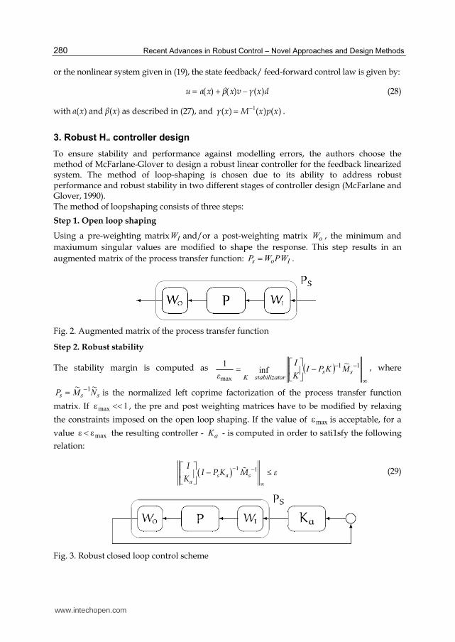
To ensure stability and performance against modelling errors, the authors choose the method of McFarlane-Glover to design a robust linear controller for the feedback linearized system. The method of loop-shaping is chosen due to its ability to address robust performance and robust stability in two different stages of controller design (McFarlane and Glover, 1990). The method of loopshaping consists of three steps:

Step 1. Open loop shaping

Using a pre-weighting matrix IW and/or a post-weighting matrix oW , the minimum and

maxiumum singular values are modified to shape the response. This step results in an

augmented matrix of the process transfer function: Ios WPWP = .

Fig. 2. Augmented matrix of the process transfer function

Step 2. Robust stability

The stability margin is computed as ( )∞

−−−⎥⎦⎤⎢⎣

⎡= 11

max

~inf

1ss

orstabilizatK

MKPIK

I

ε, where

sss NMP~~ 1−= is the normalized left coprime factorization of the process transfer function

matrix. If 1max <<ε , the pre and post weighting matrices have to be modified by relaxing

the constraints imposed on the open loop shaping. If the value of maxε is acceptable, for a

value maxε<ε the resulting controller - aK - is computed in order to sati1sfy the following

relation:

( ) 1 1s a s

a

II P K M ε

K

− −∞

⎡ ⎤ − ≤⎢ ⎥⎣ ⎦# (29)

Fig. 3. Robust closed loop control scheme

www.intechopen.com


281

Step 3. Final robust controller

The final resulting controller is given by the sub-optimal controller aK weighted with the

matrices IW and/or oW : oaI WK WK = .

Using the McFarlane-Glover method, the loop shaping is done without considering the

problem of robust stability, which is explcitily taken into account at the second design step,

by imposing a stability margin for the closed loop system. This stability margin maxε is an

indicator of the efficiency of the loopshaping technique.

Fig. 4. Optimal controller obtained with the pre and post weighting matrices

The stability of the closed loop nonlinear system using robust stability and loopshaping is proven theoretically using W-stability (Guillard & Bourles, 2000; Franco et al., 2006).

4. Case study: Reference tracking and disturbance rejection in an isothermal CSTR

The authors propose as an example, the control of an isothermal CSTR. A complete description of the steps required to obtain the final feedback linearization control scheme - in both approaches – is given. The robustness of the final nonlinear H∞ controller is demonstrated through simulations concerning reference tracking and disturbance rejection, for the robust feedback linearization case.

4.1 The isothermal continuous stirred tank reactor

The application studied is an isothermal continuous stirred tank reactor process with first

order reaction:

A B P+ → (30)

Different strategies have been proposed for this type of multivariable process (De Oliveira,

1994; Martinsen et al., 2004; Chen et al., 2010). The choice of the CSTR resides in its strong

nonlinear character, which makes the application of a nonlinear control strategy based

directly on the nonlinear model of the process preferable to classical linearization methods

(De Oliveira, 1994).

The schematic representation of the process is given in Figure 5.

The tank reactor is assumed to be a well mixed one. The control system designed for such a

process is intended to keep the liquid level in the tank – x1- constant, as well as the B

product concentration – x2, extracted at the bottom of the tank. It is also assumed that the

output flow rate Fo is determined by the liquid level in the reactor. The final concentration x2

is obtained by mixing two input streams: a concentrated one u1, of concentration CB1 and a

diluted one u2, of concentration CB2. The process is therefore modelled as a multivariable

system, having two manipulated variables, u = [u1 u2]T and two control outputs: x = [x1 x2]T.

www.intechopen.com


282

The process model is then given as:

( ) ( ) ( )1

1 2 1 1

2 1 2 2 21 2 2 2 2

1 1 21B B

dxu u k x

dtdx u u k x

C x C xdt x x x

= + −= − + − − +

(31)

with the parameters’ nominal values given in table 1. The steady state operating conditions are taken as x1ss=100 and x2ss=7.07, corresponding to the input flow rates: u1s =1 and u2s =1. The concentrations of B in the input streams, CB1 and CB2, are regarded as input disturbances.

Fig. 5. Continuous stirred tank reactor (De Oliveira, 1994)

Parameter Meaning Nominal Value

CB1 Concentration of B in the

inlet flow u124.9

CB2 Concentration of B in the

inlet flow u20.1

k1 Valve constant 0.2

k2 Kinetic constant 1

Table 1. CSTR parameters and nominal values

From a feedback linearization point of view the process model given in (31) is rewritten as:

( ) ( ) ( )[ ]

1 11

1 22 2 1 2 2 22 2

1 12

1 2

1 1

1

B B

T

k xx

u uk x C x C xx

x xx

y x x

⎛ ⎞− ⎛ ⎞ ⎛ ⎞⎜ ⎟⎛ ⎞ ⎜ ⎟ ⎜ ⎟= + +− −⎜ ⎟⎜ ⎟ ⎜ ⎟ ⎜ ⎟−⎝ ⎠ ⎜ ⎟ ⎜ ⎟ ⎜ ⎟+ ⎝ ⎠ ⎝ ⎠⎝ ⎠=

$$ (32)

www.intechopen.com


283

yielding:

11 1 2 2

2

1 1 1

2 2 2

( ) ( ) ( )

( )

( )

xf x g x u g x u

x

y h x x

y h x x

⎛ ⎞ = + +⎜ ⎟⎝ ⎠= == =

$$

(33)

The relative degrees of each output are obtained based on differentiation:

( )( ) ( )1 1 1 1 2

1 2 2 22 22 1 22

1 121

B B

y k x u u

C x C xk xy u u

x xx

= − + +− −= − + ++

$

$ (34)

thus yielding r1=1 and r2=1, respectively, with r1 + r2 = 2, the number of state variables of the nonlinear system (32). Since this is the case, the linearization will be exact, without any state variables rendered unobservable through feedback linearization. The decoupling matrix M(x) in (13), will be equal to:

( ) ( )( ) ( ) ( ) ( )1 2

1 2

0 01 2

1 2 1 20 01 2

1 1

1 1

( )g f g f

B B

g f g f

L L h L L hM x C x C x

L L h L L h x x

⎡ ⎤⎡ ⎤ ⎢ ⎥⎢ ⎥= = − −⎢ ⎥⎢ ⎥ ⎢ ⎥⎢ ⎥⎣ ⎦ ⎣ ⎦ (35)

and is non-singular in the equilibrium point x0 = [100; 7.07]T. The state transformation is given by:

[ ] [ ]1 2 1 2

T Tcx y y x x= = (36)

while the control signal vector is:

111 1

12

( ) ( ) ( ) ( )f

c c

f

L hu M x M x v x x v

L hα β− −⎡ ⎤⎢ ⎥= − + = +⎢ ⎥⎣ ⎦

(37)

with ( ) ( ) ( )1

1 1

2 21 2 1 22

1 1 2

1 1

1

( )c B B

k x

x k xC x C x

x x x

α− ⎡ ⎤−⎡ ⎤ ⎢ ⎥⎢ ⎥= − − − ⎢ ⎥⎢ ⎥ −⎢ ⎥⎢ ⎥ +⎣ ⎦ ⎣ ⎦

and ( ) ( )1

1 2 1 2

1 1

1 1

( )c B Bx C x C x

x x

β−⎡ ⎤⎢ ⎥= − −⎢ ⎥⎢ ⎥⎣ ⎦

.

In the next step, the L, T and R matrices needed for the robust feedback linearization method are computed:

0 0

0-1

-2 -2

-0.1 10( ) ( )

-0.11 10 -0.84 10x cL M x ┙ x

⎛ ⎞⋅⎜ ⎟= − ∂ = ⎜ ⎟⋅ ⋅⎝ ⎠ (38)

0

1 0

0 1( )x cT x x

⎛ ⎞= ∂ = ⎜ ⎟⎝ ⎠ (39)

www.intechopen.com


284

1

0(0.28 4.03

)0.72 -4.03

R M x− ⎛ ⎞= = ⎜ ⎟⎝ ⎠ (40)

The control law can be easily obtained based on (27) as:

1

1

( ) ( ) ( )

( ) ( )

c c c

c

┙ x ┙ x ┚ x LT x

┚ x ┚ x R

−−

= += (41)

while the linearized system is given as:

( )( )

1 2110

1 22 20

3

20

0 1 12

7 07 7 0710 100 100

1

/

. .B B

kx

z z wC Ck x

x

−⎛ ⎞−⎜ ⎟ ⎛ ⎞⎜ ⎟⎜ ⎟= + − −− ⎜ ⎟⎜ ⎟ ⎜ ⎟⎜ ⎟ ⎝ ⎠⎜ ⎟+⎝ ⎠$ (42)

The linear H∞ controller is designed using the McFarlane-Glover method (McFarlane, et al.,

1989; Skogestad, et al., 2007) with loop-shaping that ensures the robust stabilization problem

of uncertain linear plants, given by a normalized left co-prime factorization. The loop-

shaping ( ) ( ) ( )sP s W s P s= , with P(s) the matrix transfer function of the linear system given in

(41), is done with the weighting matrix, W:

14 10

W diags s

⎛ ⎞= ⎜ ⎟⎝ ⎠ (43)

The choice of the weighting matrix corresponds to the performance criteria that need to be

met. Despite robust stability, achieved by using a robust ∞H controller, all process outputs

need to be maintained at their set-point values. To keep the outputs at the prescribed set-

points, the steady state errors have to be reduced. The choice of the integrators in the

weighting matrix W above ensure the minimization of the output signals steady state errors.

To keep the controller as simple as possible, only a pre-weighting matrix is used (Skogestad,

et al., 2007). The resulting robust controller provides for a robustness of 38%, corresponding

to a value of 2.62=ε .

The simulation results considering both nominal values as well as modelling uncertainties

are given in Figure 6. The results obtained using the designed nonlinear controller show that

the closed loop control scheme is robust, the uncertainty range considered being of ±20% for

k1 and ±30% for k2.

A different case scenario is considered in Figure 7, in which the input disturbances CB1 and

CB2 have a +20% deviation from the nominal values. The simulation results show that the

nonlinear robust controller, apart from its robustness properties, is also able to reject input

disturbances.

To test the output disturbance rejection situation, the authors consider an empiric model of a

measurable disturbance that has a direct effect on the output vector. To consider a general

situation from a feedback linearization perspective, the nonlinear model in (33) is altered to

model the disturbance, d(t), as:

www.intechopen.com


285

0 1 2 3 4 5 695

96

97

98

99

100

101

102

Time

x1

uncertain case

nominal case

a) b)

0 1 2 3 4 5 60

2

4

6

8

10

12

Time

u1

uncertain case

nominal case

0 1 2 3 4 5 60

1

2

3

4

5

6

7

Time

u2

uncertain case

nominal case

c) d)

Fig. 6. Closed loop simulations using robust nonlinear controller a) x1 b) x2 c) u1 d) u2

11 1 2 2

2

1 1 1

2 2 2

( ) ( ) ( ) ( )

( )

( )

xf x g x u g x u p x d

x

y h x x

y h x x

⎛ ⎞ = + + +⎜ ⎟⎝ ⎠= == =

$$

(44)

with p(x) taken to be dependent on the output vector:

1

2

( )x

p xx

⎛ ⎞= ⎜ ⎟⎝ ⎠ (45)

The relative degrees of the disturbance to the outputs of interest are: 1 1γ = and 2 1γ = . Since

the relative degrees of the disturbances to the outputs are equal to those of the inputs, a

simple static feed-forward structure can be used for output disturbance rejection purposes,

with the control law given in (28), with )(xα and )(xく determined according to (27) and

)(xけ being equal to:

0 1 2 3 4 5 66.5

6.6

6.7

6.8

6.9

7

7.1

7.2

7.3

Time

x2

uncertain case

nominal case

www.intechopen.com


286

( ) ( )1

111 2 1 2

2

1 1

1 1

( ) ( ) ( ) B B

x┛ x M x p x C x C x

xx x

−−

⎡ ⎤ ⎛ ⎞⎢ ⎥= = − − ⎜ ⎟⎢ ⎥ ⎝ ⎠⎢ ⎥⎣ ⎦ (46)

0 1 2 3 4 5 695

96

97

98

99

100

101

102

Time

x1

input disturbance

no disturbance

0 1 2 3 4 5 66.5

6.6

6.7

6.8

6.9

7

7.1

7.2

7.3

7.4

7.5

Time

x2

input disturbance

no disturbance

a) b)

0 1 2 3 4 5 60

2

4

6

8

10

12

Time

u1

input disturbance

no disturbance

0 1 2 3 4 5 60

1

2

3

4

5

6

7

Time

u2

input disturbance

no disturbance

c) d)

Fig. 7. Input disturbance rejection using robust nonlinear controller a) x1 b) x2 c) u1 d) u2

The simulation results considering a unit disturbance d are given in Figure 8, considering a time delay in the sensor measurements of 1 minute. The results show that the state feedback/feed-forward scheme proposed in the robust feedback linearization framework is able to reject measurable output disturbances. A comparative simulation is given considering the case of no feed-forward scheme. The results show that the use of the feed-forward scheme in the feedback linearization loop reduces the oscillations in the output, with the expense of an increased control effort. In the unlikely situation of no time delay measurements of the disturbance d, the results obtained using feed-forward compensator are highly notable, as compared to the situation without the compensator. The simulation results are given in Figure 9. Both, Figure 8 and Figure 9 show the efficiency of such feed-forward control scheme in output disturbance rejection problems.

www.intechopen.com


287

0 2 4 6 8 10 12 14 16 18 2075

80

85

90

95

100

105

110

115

120

125

Time

x1

without compensator

with compensator

0 2 4 6 8 10 12 14 16 18 203

4

5

6

7

8

9

10

Time

x2

without compensator

with compensator

a) b)

0 2 4 6 8 10 12 14 16 18 20-120

-100

-80

-60

-40

-20

0

20

Time

u1

without compensator

with compensator

0 2 4 6 8 10 12 14 16 18 20-140

-120

-100

-80

-60

-40

-20

0

20

Time

u2

without compensator

with compensator

c) d)

Fig. 8. Output disturbance rejection using robust nonlinear controller and feed-forward compensator considering time delay measurements of the disturbance d a) x1 b) x2 c) u1 d) u2

5. Conclusions

As it has been previously demonstrated theoretically through mathematical computations

(Guillard, et al., 2000), the results in this paper prove that by combining the robust method

of feedback linearization with a robust linear controller, the robustness properties are kept

when simulating the closed loop nonlinear uncertain system. Additionally, the design of the

loop-shaping controller is significantly simplified as compared to the classical linearization

technique, since the final linearized model bears significant information regarding the initial

nonlinear model. Finally, the authors show that robust nonlinear controller - designed by

combining this new method for feedback linearization (Guillard & Bourles, 2000) with a

linear H∞ controller - offers a simple and efficient solution, both in terms of reference

tracking and input disturbance rejection. Moreover, the implementation of the feed-forward

control scheme in the state-feedback control structure leads to improved output disturbance

rejection.

www.intechopen.com


288

0 5 10 15 2095

100

105

110

115

120

125

Time

x1

with compensator

without compensator

0 5 10 15 203

4

5

6

7

8

9

10

Time

x2

with compensator

without compensator

a) b)

0 5 10 15 20-120

-100

-80

-60

-40

-20

0

20

Time

u1

with compensator

without compensator

0 5 10 15 20-80

-70

-60

-50

-40

-30

-20

-10

0

10

Time

u2

with compensator

without compensator

c) d)

Fig. 9. Output disturbance rejection using robust nonlinear controller and feed-forward compensator considering instant measurements of the disturbance d a) x1 b) x2 c) u1 d) u2

6. References

Barkhordari Yazdi, M., & Jahed-Motlagh, M.R. (2009), Stabilization of a CSTR with two

arbitrarily switching modes using modal state feedback linearization, In: Chemical

Engineering Journal, vol. 155, pp. 838-843, ISSN: 1385-8947

Chen, P., Lu, I.-Z., & Chen, Y.-W. (2010), Extremal Optimization Combined with LM

Gradient Search for MLP Network Learning, International Journal of Computational

Intelligence Systems, Vol.3, No. 5, pp. 622-631, ISSN: 1875-6891

Chou, YI-S., & Wu, W. (1995), Robust controller design for uncertain nonlinear systems via

feedback linearization, In: Chemical Engineering Science, vol. 50, No. 9, pp. 1429-1439,

ISSN: 0009-2509

Dabo, M., Langlois, & N., Chafouk, H. (2009), Dynamic feedback linearization applied to

asymptotic tracking: Generalization about the turbocharged diesel engine outputs

www.intechopen.com


289

choice, In: Proceedings of the American Control Conference ACC’09, ISBN: 978-1-4244-

4524-0, pp. 3458 – 3463, St. Louis, Missouri, USA, 10-12 June 2009

Daoutidis, P., & Kravaris, C. (1989), Synthesis of feedforward/state feedback controllers for

nonlinear processes, In: AIChE Journal, vol. 35, pp.1602–1616, ISSN: 1547-5905

Daoutidis, P., Soruosh, M, & Kravaris, C. (1990), Feedforward-Feedback Control of

Multivariable Nonlinear Processes, In: AIChE Journal, vol. 36, no.10, pp.1471–1484,

ISSN: 1547-5905

Franco, A.L.D., Bourles, H., De Pieri, E.R., & Guillard, H. (2006), Robust nonlinear control

associating robust feedback linearization and ∞H control, In: IEEE Transactions on

Automatic Control, vol. 51, No. 7, pp. 1200-1207, ISSN: 0018-9286

Franco, A.L.D., Bourles, H., & De Pieri, E.R. (2005), A robust nonlinear controller with

application to a magnetic bearing, In: Proceedings of the 44th IEEE Conference on

Decision and Control and The European Control Conference, ISBN: 0-7803-9567-0,

Seville, Spain, 12-15 December 2005

Guillard, H., &Bourles, H. (2000), Robust feedback linearization, In: Proc. 14 th International

Symposium on Mathematical Theory of Networks and Systems, Perpignan, France, 19-23

June 2000

Isidori, A. (1995), Nonlinear control systems, Springer-Verlag, ISBN: 3540199160, New York,

USA

Martinesn, F., Biegler, L. T., & Foss, B. A. (2004), A new optimization algorithm with

application to nonlinear MPC, Journal of Process Control, vol. 14, No. 8, pp. 853-865,

ISSN: 0959-1524

McFarlane, D.C, & Glover, K. (1990), Robust controller design using normalized coprime

factor plant descriptions, In: Lecture Notes in Control and Information Sciences, vol.

138, Springer Verlag, New York, USA, ISSN: 0170-8643

De Oliveira, N. M. C (1994), Newton type algorithms for nonlinear constrained chemical process

control, PhD thesis, Carnegie Melon University, Pennsylvania

Pop, C.I, Dulf, E., & Festila, Cl. (2009), Nonlinear Robust Control of the 13C Cryogenic

Isotope Separation Column, In: Proceedings of the 17th International Conference on

Control Systems and Computer Science, Vol.2., pp.59-65, ISSN: 2066-4451, Bucharest,

Romania, 26-29 May 2009

Pop, C.-I., & Dulf, E.-H. (2010), Control Strategies of the 13C Cryogenic Separation Column,

Control Engineering and Applied Informatics, Vol. 12, No. 2, pp.36-43, June 2010, ISSN

1454-8658

Pop, C.I., Dulf, E., Festila, Cl., & Muresan, B. (2010), Feedback Linearization Control Design

for the 13C Cryogenic Separation Column, In: International IEEE-TTTC International

Conference on Automation, Quality and Testing, Robotics AQTR 2010, vol. I, pp. 157-

163, ISBN: 978-1-4244-6724-2, Cluj-Napoca, Romania, 28-30 May 2010

Robenack, K. (2005), Automatic differentiation and nonlinear controller design by exact

linearization, In: Future Generation Computer Systems, vol. 21, pp. 1372-1379, ISSN:

0167-739X

Seo, J., Venugopala, & R., Kenne, J.-P. (2007), Feedback linearization based control of a

rotational hydraulic drive, In: Control Engineering Practice, vol. 15, pp. 1495–1507,

ISSN: 0967-0661

www.intechopen.com


290

Sastry, S. S. (1999), Nonlinear systems: analysis, stability and control, Springer Verlag, ISBN: 0-

387-98513-1, New York, USA

Henson, M., & Seborg, D. (Eds.),(1997), Nonlinear process control, Prentice Hall, ISBN: 978-

0136251798, New York, USA

www.intechopen.com

Recent Advances in Robust Control - Novel Approaches andDesign MethodsEdited by Dr. Andreas Mueller

ISBN 978-953-307-339-2Hard cover, 462 pagesPublisher InTechPublished online 07, November, 2011Published in print edition November, 2011

InTech EuropeUniversity Campus STeP Ri Slavka Krautzeka 83/A 51000 Rijeka, Croatia Phone: +385 (51) 770 447 Fax: +385 (51) 686 166www.intechopen.com

InTech ChinaUnit 405, Office Block, Hotel Equatorial Shanghai No.65, Yan An Road (West), Shanghai, 200040, China

Phone: +86-21-62489820 Fax: +86-21-62489821

Robust control has been a topic of active research in the last three decades culminating in H_2/H_\infty and\mu design methods followed by research on parametric robustness, initially motivated by Kharitonov'stheorem, the extension to non-linear time delay systems, and other more recent methods. The two volumes ofRecent Advances in Robust Control give a selective overview of recent theoretical developments and presentselected application examples. The volumes comprise 39 contributions covering various theoretical aspects aswell as different application areas. The first volume covers selected problems in the theory of robust controland its application to robotic and electromechanical systems. The second volume is dedicated to special topicsin robust control and problem specific solutions. Recent Advances in Robust Control will be a valuablereference for those interested in the recent theoretical advances and for researchers working in the broad fieldof robotics and mechatronics.

How to referenceIn order to correctly reference this scholarly work, feel free to copy and paste the following:

Cristina Ioana Pop and Eva Henrietta Dulf (2011). Robust Feedback Linearization Control for ReferenceTracking and Disturbance Rejection in Nonlinear Systems, Recent Advances in Robust Control - NovelApproaches and Design Methods, Dr. Andreas Mueller (Ed.), ISBN: 978-953-307-339-2, InTech, Availablefrom: http://www.intechopen.com/books/recent-advances-in-robust-control-novel-approaches-and-design-methods/robust-feedback-linearization-control-for-reference-tracking-and-disturbance-rejection-in-nonlinear-

robust feedback linearization control for reference ......section 3 presents theh∞robust...

Documents