robust design - missouri university of science and …web.mst.edu/~dux/repository/me261/robust...
TRANSCRIPT

Robust Design
ME 261 Engineering Design 2014 Spring Xiaoping Du

Outline
• Introductory Examples
• Definition of Robustness
• Statistics
• How to achieve robustness
• Examples
• Related Issue: Reliability
• Conclusions 2
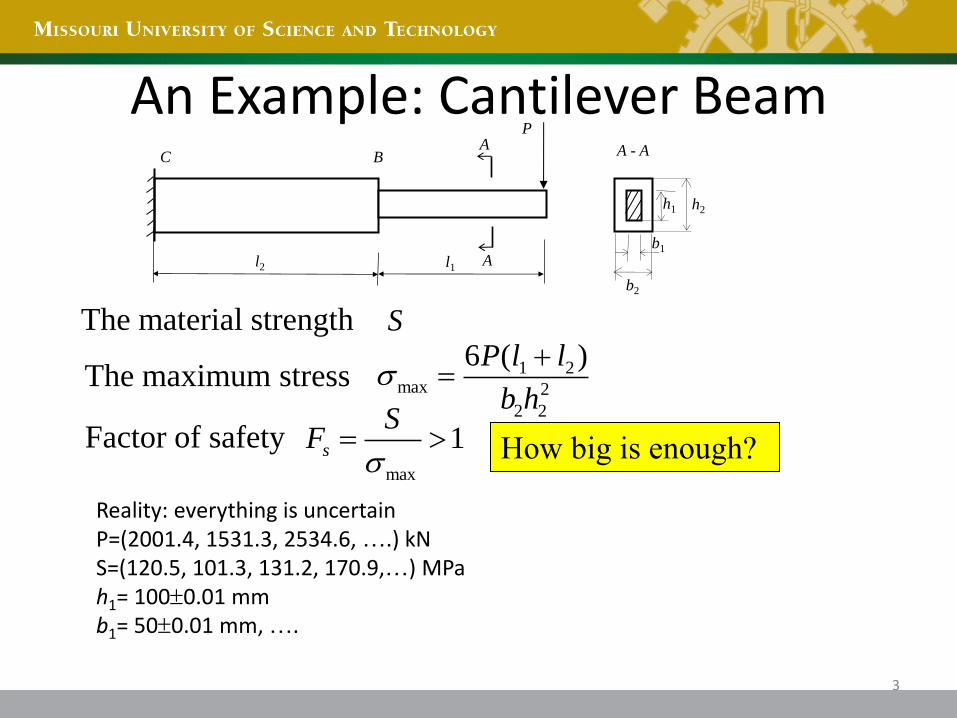
An Example: Cantilever Beam
3
h1 h2
b2
b1
l2 l1
P A
A
A - A B C
The maximum stress 1 2max 2
2 2
6 ( )P l l
b h
The material strength S
Factor of safety max
1s
SF
Reality: everything is uncertain P=(2001.4, 1531.3, 2534.6, ….) kN S=(120.5, 101.3, 131.2, 170.9,…) MPa h1= 1000.01 mm b1= 500.01 mm, ….
How big is enough?

Which Design is Robust Under Uncertainty?
4
Sensitive to variation Robust
Increased Robustness

Variation (Uncertainty)
• Piece-to-piece variation
• Customer usage and duty cycle
• Human errors
• Model inaccuracy
5
Uncertainty
Present state of
knowledge
Complete
ignorance
Knowledge
Complete
knowledge

How Do We Quantify Uncertainty? • Support we have 100 measurements for 𝑋 = 𝐿1
• (99.99, 100.08,…,100.05) mm
6
100
1
1Mean 99.96
100i
i
X x
Average
2
1
1Standard deviation ( )
100 1
n
i
i
x X
Dispersion
Histogram Probability density (distribution)

Probability Distribution • Mean – average • Standard deviation (std) –
dispersion around the average or amount of variation
• Two designs with two performance variables
• 𝑋 1 = 𝑋 2, 𝜎2 > 𝜎1 • Designs 1 and 2 have the same
average performance • But the variation of Design 2 is
higher.
7
Design 1
𝑋 1, 𝜎1
Design 2
𝑋 2, 𝜎2
𝑋 1
𝑋 2
Concept of Robustness
8
Big or dangerous?
Robustness
• The robustness of a product is the ability that its performances are not affected by the uncertain inputs or environment conditions (noises).
• A robust product can work under large uncertainties.
9
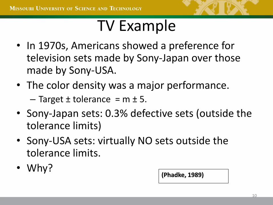
TV Example • In 1970s, Americans showed a preference for
television sets made by Sony-Japan over those made by Sony-USA.
• The color density was a major performance. – Target ± tolerance = m ± 5.
• Sony-Japan sets: 0.3% defective sets (outside the tolerance limits)
• Sony-USA sets: virtually NO sets outside the tolerance limits.
• Why?
10
(Phadke, 1989)

TV Example
• Sony-USA: Uniform distribution, σ = 2.89
• Sony-Japan: Normal distribution, σ = 1.67, and most of the sets are grade A.
11
(Phadke, 1989)
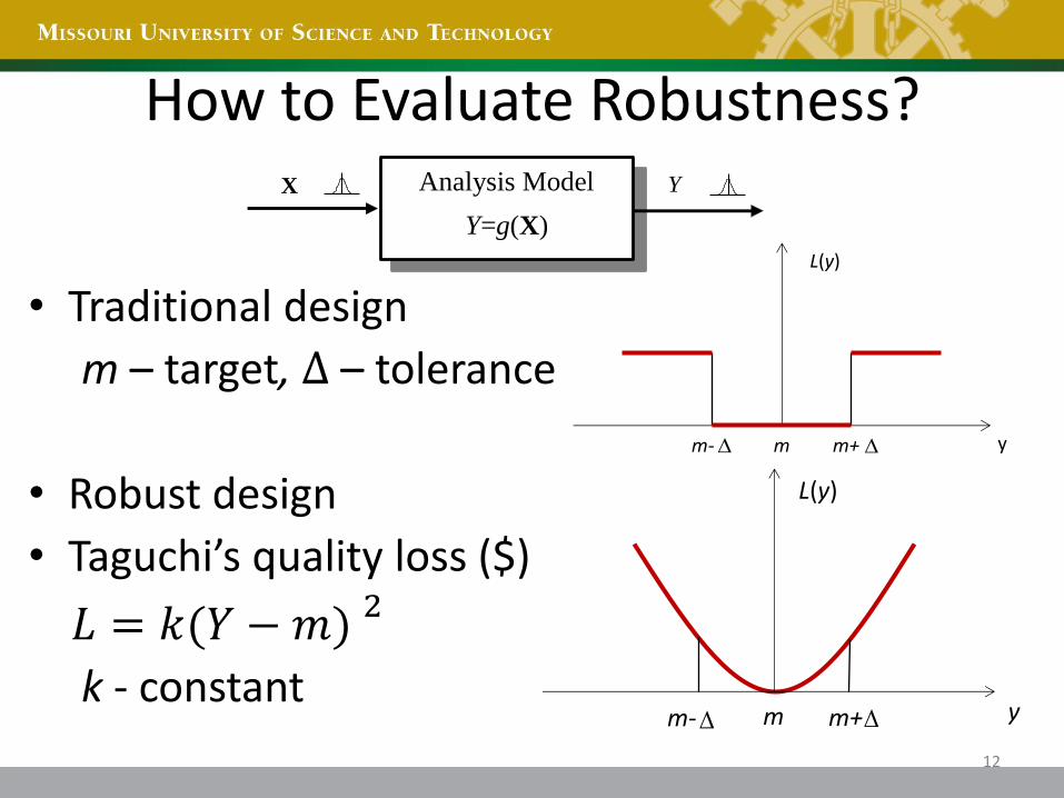
How to Evaluate Robustness?
• Traditional design
m – target, ∆ – tolerance
• Robust design
• Taguchi’s quality loss ($)
𝐿 = 𝑘(𝑌 −𝑚) 2
k - constant
12
Analysis Model
Y=g(X)
X Y
L(y)
m m- m+ y
L(y)
y m m- m+

Expected Quality Loss • Expected (average) quality loss
E(𝐿) = 𝑘[ 𝑌 − 𝑚 2+ 𝜎𝑌
2]
• Reducing E 𝐿 will bring the average performance to the target and reducing variation 𝜎𝑌 simultaneously.
13
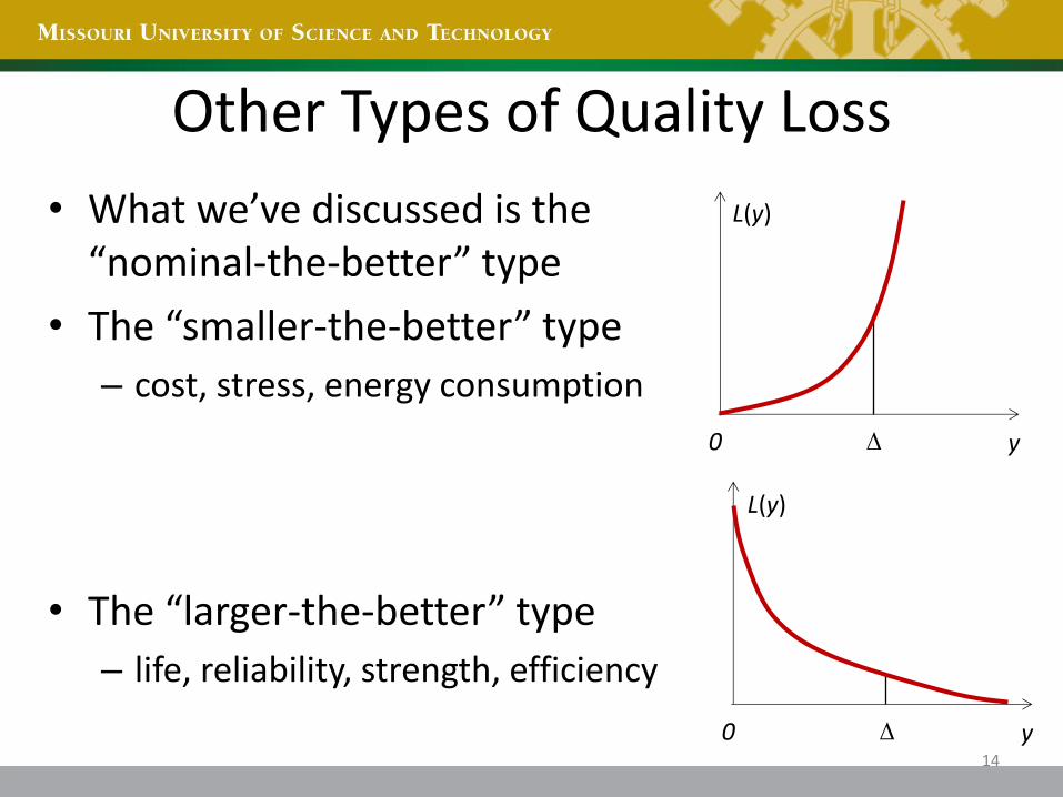
Other Types of Quality Loss
• What we’ve discussed is the “nominal-the-better” type
• The “smaller-the-better” type
– cost, stress, energy consumption
• The “larger-the-better” type
– life, reliability, strength, efficiency
14
y
L(y)
0
y
L(y)
0

Robust Design
15
Decreasing variation
Incr
easi
ng
aver
age
per
form
ance

Achieve Robustness During Conceptual Design
• Keep uncertainty in mind
• Define the robustness target
• Identify the root causes of variations
• Make design concepts not sensitive to variations in later design stages, manufacturing, and operation. – For example, if the fluctuation in temperature is
high, use a pair of gears instead of a belt.
16

Achieve Robustness During Parameter Design
• Performance 𝑌 = 𝑔 𝑋1, 𝑋2, … , 𝑋𝑛
• Design variables 𝐗 = 𝑋 1, 𝑋 2, … , 𝑋 𝑛
• 𝑋𝑖 𝑖 = 1,2,⋯ , 𝑛 are independent
17
X
Y
0

Parameter Design • Average performance 𝑌 = 𝑓 𝑋 1, 𝑋 2, … , 𝑋 𝑛
• Taylor expansion series • 𝑌 ≈ 𝑌 + 𝑐1(𝑋1−𝑋 1) + 𝑐2(𝑋2−𝑋 2) +⋯+ 𝑐𝑛(𝑋𝑛 − 𝑋 𝑛)
• 𝑐𝑖 =𝜕𝑔
𝜕𝑋𝑖 at 𝐗 𝑖 = 1,2,⋯ , 𝑛
• Std 𝜎𝑌 = 𝑐12𝜎1
2 + 𝑐22𝜎2
2 +⋯+ 𝑐𝑛2𝜎𝑛
2 • Change 𝐗 (not reduce 𝜎𝑖) to reduce (or
minimize)
E(𝐿) = 𝑘[ 𝑌 − 𝑚 2+ 𝜎𝑌
2]
18
Taylor expansion
X
Y
0 X

Example: Robust Mechanism Synthesis
19
• Requirements:
𝑠 = 𝑚1 = 350 mm when 𝜃 = 10 𝑠 = 𝑚2 = 250 mm when 𝜃 = 60
• Uncertainties in a, b, and e
𝜎𝑎 = 2 mm, 𝜎𝑏 = 2 mm,𝜎𝑒 = 3 mm
• Design variables
𝑎 , 𝑏 , 𝑒 a b
e
A
N N C
B

Results
20
Method Deterministic Design Robust Design
𝑎 (mm) 119.6 136.6
𝑏 (mm) 241.3 216.8
𝑒 (mm) 45.0 0.0
𝑠 (𝜃 = 10) (mm) 350 350
𝑠 (𝜃 = 60) (mm) 250 250
σ (𝜃 = 10) (mm) 2.9 2.8
σ (𝜃 = 60) (mm) 3.5 3.1
22cos sins a b e a
Minimize 𝑘[ 𝑠 𝑖 −𝑚𝑖 2+ 𝜎𝑠𝑖
22𝑖=1 ]
Transmission angle > 45
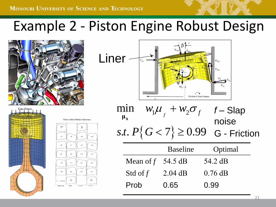
Example 2 - Piston Engine Robust Design
21
Baseline Optimal
Mean of f 54.5 dB 54.2 dB
Std of f 2.04 dB 0.76 dB
Prob 0.65 0.99
Liner
1 2min
. . 7 0.99
f fw w
s t P G
xμf – Slap
noise
G - Friction
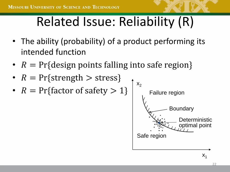
Related Issue: Reliability (R)
• The ability (probability) of a product performing its intended function
• 𝑅 = Pr {design points falling into safe region}
• 𝑅 = Pr {strength > stress}
• 𝑅 = Pr {factor of safety > 1}
22
x1
Failure region
Safe region
Boundary
x2
Deterministic optimal point
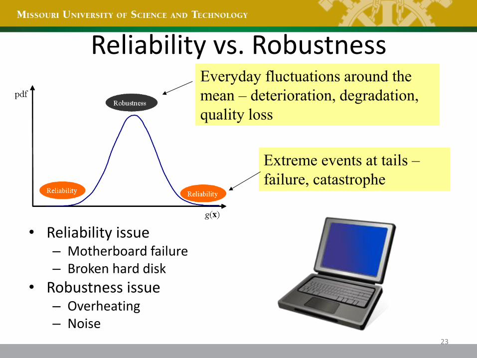
Reliability vs. Robustness
23
Everyday fluctuations around the
mean – deterioration, degradation,
quality loss
Extreme events at tails –
failure, catastrophe
• Reliability issue – Motherboard failure – Broken hard disk
• Robustness issue – Overheating – Noise
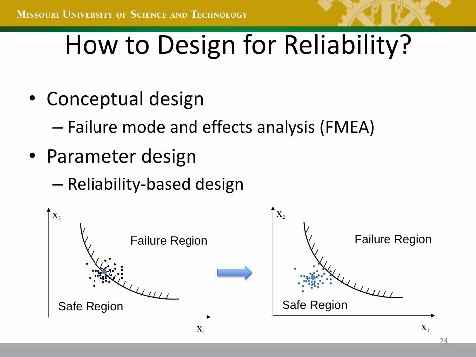
How to Design for Reliability?
• Conceptual design
– Failure mode and effects analysis (FMEA)
• Parameter design
– Reliability-based design
24
x2
x1
Failure Region
Safe Region
x2
x1
Failure Region
Safe Region
Conclusions
• Robust design -> insensitivity to uncertainties – Insensitive to material variations-> use of low grade
materials and components -> low material cost – Insensitive to manufacturing variations -> no
tightened tolerances -> low manufacturing and labor cost
– Insensitive to variations in operation environment -> low operation cost
• Robust design -> increased performance, quality, and reliability at reduced cost
• Robustness and reliability can be built into products during early stages of design.
25
More Information
• Visit the website of Engineering Uncertainty Repository at http://www.mst.edu/~dux/repository.
• Contact me for any help in Toomey Hall 290D or at [email protected].
26