robust control toolbox user's guide
TRANSCRIPT

7/30/2019 Robust Control Toolbox User's Guide
http://slidepdf.com/reader/full/robust-control-toolbox-users-guide 1/180
Robust Control Toolbox™
User’s Guide
R2012a
Gary BalasRichard Chia ng
Andy Packard Michael Safonov
7/30/2019 Robust Control Toolbox User's Guide
http://slidepdf.com/reader/full/robust-control-toolbox-users-guide 2/180
How to Contact MathWorks
www.mathworks.com Web
comp.soft-sys.matlab Newsgroup
www.mathworks.com/contact_TS.html Technical Support
[email protected] Product enhancement suggestions
[email protected] Bug reports
[email protected] Documentation error reports
[email protected] Order status, license renewals, passcodes
[email protected] Sales, pricing, and general information
508-647-7000 (Phone)
508-647-7001 (Fax)
The MathWorks, Inc.
3 Apple Hill DriveNatick, MA 01760-2098
For contact information about worldwide offices, see the MathWorks Web site.
Robust Control Toolbox™ User’s Guide
© COPYRIGHT 2005–2012 by The MathWorks, Inc.
The software described in this document is furnished under a license agreement. The software may be usedor copied only under the terms of the license agreement. No part of this manual may be photocopied orreproduced in any form without prior written consent from The MathWorks, Inc.
FEDERAL ACQUISITION: This provision applies to all acquisitions of the Program and Documentationby, for, or through the federal government of the United States. By accepting delivery of the Programor Documentation, the government hereby agrees that this software or documentation qualifies ascommercial computer software or commercial computer software documentation as such terms are usedor defined in FAR 12.212, DFARS Part 227.72, and DFARS 252.227-7014. Accordingly, the terms andconditions of this Agreement and only those rights specified in this Agreement, shall pertain to and governthe use, modification, reproduction, release, performance, display, and disclosure of the Program andDocumentation by the federal government (or other entity acquiring for or through the federal government)and shall supersede any conflicting contractual terms or conditions. If this License fails to meet thegovernment’s needs or is inconsistent in any respect with federal procurement law, the government agreesto return the Program and Documentation, unused, to The MathWorks, Inc.
Trademarks
MATLAB and Simulink are registered trademarks of The MathWorks, Inc. Seewww.mathworks.com/trademarks for a list of additional trademarks. Other product or brandnames may be trademarks or registered trademarks of their respective holders.
Patents
MathWorks products are protected by one or more U.S. patents. Please seewww.mathworks.com/patents for more information.

7/30/2019 Robust Control Toolbox User's Guide
http://slidepdf.com/reader/full/robust-control-toolbox-users-guide 3/180
Revision History
September 2005 First printing New for Version 3.0.2 (Release 14SP3)
March 2006 Online only Revised for Version 3.1 (Release 2006a)September 2006 Online only Revised for Version 3.1.1 (Release 2006b)March 2007 Online only Revised for Version 3.2 (Release 2007a)September 2007 Online only Revised for Version 3.3 (Release 2007b)March 2008 Online only Revised for Version 3.3.1 (Release 2008a)October 2008 Online only Revised for Version 3.3.2 (Release 2008b)March 2009 Online only Revised for Version 3.3.3 (Release 2009a)September 2009 Online only Revised for Version 3.4 (Release 2009b)March 2010 Online only Revised for Version 3.4.1 (Release 2010a)September 2010 Online only Revised for Version 3.5 (Release 2010b) April 2011 Online only Revised for Version 3.6 (Release 2011a)
September 2011 Online only Revised for Version 4.0 (Release 2011b)March 2012 Online only Revised for Version 4.1 (Release 2012a)

7/30/2019 Robust Control Toolbox User's Guide
http://slidepdf.com/reader/full/robust-control-toolbox-users-guide 4/180

7/30/2019 Robust Control Toolbox User's Guide
http://slidepdf.com/reader/full/robust-control-toolbox-users-guide 5/180
Contents
Building Uncertain Models
Introduction to Uncertain Atoms . . . . . . . . . . . . . . . . . . . . 1-2
Uncertain Real Parameters . . . . . . . . . . . . . . . . . . . . . . . . . 1-3
Uncertain LTI Dynamics Atoms . . . . . . . . . . . . . . . . . . . . . 1-10
Complex Parameter Atoms . . . . . . . . . . . . . . . . . . . . . . . . . . 1-13
Complex Matrix Atoms . . . . . . . . . . . . . . . . . . . . . . . . . . . . . 1-15Unstructured Uncertain Dynamic Systems . . . . . . . . . . . . 1-17
Uncertain Matrices . . . . . . . . . . . . . . . . . . . . . . . . . . . . . . . . 1-19
Creating Uncertain Matrices from Uncertain Atoms . . . . . 1-19
Accessing Properties of a umat . . . . . . . . . . . . . . . . . . . . . . . 1-20
Row and Column Referencing . . . . . . . . . . . . . . . . . . . . . . . 1-21
Matrix Operation on umat Objects . . . . . . . . . . . . . . . . . . . 1-22
Substituting for Uncertain Atoms . . . . . . . . . . . . . . . . . . . . 1-23
Uncertain State-Space Systems (uss) . . . . . . . . . . . . . . . . 1-26
Creating Uncertain Systems . . . . . . . . . . . . . . . . . . . . . . . . 1-26
Properties of uss Objects . . . . . . . . . . . . . . . . . . . . . . . . . . . . 1-27
Sampling Uncertain Systems . . . . . . . . . . . . . . . . . . . . . . . . 1-28
Feedback Around an Uncertain Plant . . . . . . . . . . . . . . . . . 1-29
Interpreting Uncertainty in Discrete Time . . . . . . . . . . . . . 1-31
Lifting a ss to a uss . . . . . . . . . . . . . . . . . . . . . . . . . . . . . . . . 1-32
Handling Delays in uss . . . . . . . . . . . . . . . . . . . . . . . . . . . . . 1-32
Uncertain frd . . . . . . . . . . . . . . . . . . . . . . . . . . . . . . . . . . . . . 1-35
Creating Uncertain Frequency Response Objects . . . . . . . . 1-35
Properties of ufrd Objects . . . . . . . . . . . . . . . . . . . . . . . . . . . 1-35
Interpreting Uncertainty in Discrete Time . . . . . . . . . . . . . 1-37
Lifting an frd to a ufrd . . . . . . . . . . . . . . . . . . . . . . . . . . . . . 1-38Handling Delays in ufrd . . . . . . . . . . . . . . . . . . . . . . . . . . . . 1-38
Basic Control System Toolbox and MATLAB
Interconnections . . . . . . . . . . . . . . . . . . . . . . . . . . . . . . . . 1-39
v
7/30/2019 Robust Control Toolbox User's Guide
http://slidepdf.com/reader/full/robust-control-toolbox-users-guide 6/180

7/30/2019 Robust Control Toolbox User's Guide
http://slidepdf.com/reader/full/robust-control-toolbox-users-guide 7/180
Robust Performance Margin . . . . . . . . . . . . . . . . . . . . . . . . 2-5
Worst-Case Gain Measure . . . . . . . . . . . . . . . . . . . . . . . . . . 2-6
Introduction to Linear Matrix Inequalities
Linear Matrix Inequalities . . . . . . . . . . . . . . . . . . . . . . . . . 3-2
LMI Features . . . . . . . . . . . . . . . . . . . . . . . . . . . . . . . . . . . . . 3-2
LMIs and LMI Problems . . . . . . . . . . . . . . . . . . . . . . . . . . . . 3-4
Three Generic LMI Problems . . . . . . . . . . . . . . . . . . . . . . . . 3-5
Further Mathematical Background . . . . . . . . . . . . . . . . . 3-10
Bibliography . . . . . . . . . . . . . . . . . . . . . . . . . . . . . . . . . . . . . . 3-11
LMI Lab
Introduction . . . . . . . . . . . . . . . . . . . . . . . . . . . . . . . . . . . . . . 4-2Some Terminology . . . . . . . . . . . . . . . . . . . . . . . . . . . . . . . . . 4-2
Overview of the LMI Lab . . . . . . . . . . . . . . . . . . . . . . . . . . . 4-5
Specifying a System of LMIs . . . . . . . . . . . . . . . . . . . . . . . . 4-8
A Simple Example . . . . . . . . . . . . . . . . . . . . . . . . . . . . . . . . . 4-9
Initializing the LMI System . . . . . . . . . . . . . . . . . . . . . . . . . 4-11
Specifying the LMI Variables . . . . . . . . . . . . . . . . . . . . . . . . 4-11
Specifying Individual LMIs . . . . . . . . . . . . . . . . . . . . . . . . . 4-13
Specifying LMIs with the LMI Editor . . . . . . . . . . . . . . . . . 4-16
How It All Works . . . . . . . . . . . . . . . . . . . . . . . . . . . . . . . . . . 4-19
Querying the LMI System Description . . . . . . . . . . . . . . . 4-21
lmiinfo . . . . . . . . . . . . . . . . . . . . . . . . . . . . . . . . . . . . . . . . . . 4-21
vii
7/30/2019 Robust Control Toolbox User's Guide
http://slidepdf.com/reader/full/robust-control-toolbox-users-guide 8/180
lminbr and matnbr . . . . . . . . . . . . . . . . . . . . . . . . . . . . . . . . 4-21
LMI Solvers . . . . . . . . . . . . . . . . . . . . . . . . . . . . . . . . . . . . . . . 4-22
From Decision to Matrix Variables and Vice Versa . . . 4-28
Validating Results . . . . . . . . . . . . . . . . . . . . . . . . . . . . . . . . . 4-29
Modifying a System of LMIs . . . . . . . . . . . . . . . . . . . . . . . . 4-30
Deleting an LMI . . . . . . . . . . . . . . . . . . . . . . . . . . . . . . . . . . 4-30
Deleting a Matrix Variable . . . . . . . . . . . . . . . . . . . . . . . . . . 4-30
Instantiating a Matrix Variable . . . . . . . . . . . . . . . . . . . . . . 4-31
Advanced Topics . . . . . . . . . . . . . . . . . . . . . . . . . . . . . . . . . . 4-33
Structured Matrix Variables . . . . . . . . . . . . . . . . . . . . . . . . 4-33
Complex-Valued LMIs . . . . . . . . . . . . . . . . . . . . . . . . . . . . . 4-35
Specifying cTx Objectives for mincx . . . . . . . . . . . . . . . . . . . 4-38
Feasibility Radius . . . . . . . . . . . . . . . . . . . . . . . . . . . . . . . . . 4-40
Well-Posedness Issues . . . . . . . . . . . . . . . . . . . . . . . . . . . . . 4-40
Semi-Definite B(x) in gevp Problems . . . . . . . . . . . . . . . . . . 4-41
Efficiency and Complexity Issues . . . . . . . . . . . . . . . . . . . . . 4-42
Solving M + PTXQ + QTXTP < 0 . . . . . . . . . . . . . . . . . . . . . . 4-43
Bibliography . . . . . . . . . . . . . . . . . . . . . . . . . . . . . . . . . . . . . . 4-45
Analyzing Uncertainty Effects in Simulink
Overview . . . . . . . . . . . . . . . . . . . . . . . . . . . . . . . . . . . . . . . . . 5-2
Robust Control Toolbox Block Library . . . . . . . . . . . . . . 5-4
Specifying Uncertainty Using Uncertain State Space
Blocks . . . . . . . . . . . . . . . . . . . . . . . . . . . . . . . . . . . . . . . . . . 5-5
How to Specify Uncertainty in Uncertain State Space
Blocks . . . . . . . . . . . . . . . . . . . . . . . . . . . . . . . . . . . . . . . . 5-5
Next Steps . . . . . . . . . . . . . . . . . . . . . . . . . . . . . . . . . . . . . . . 5-7
viii Contents

7/30/2019 Robust Control Toolbox User's Guide
http://slidepdf.com/reader/full/robust-control-toolbox-users-guide 9/180
Simulating Uncertainty Effects . . . . . . . . . . . . . . . . . . . . . 5-8
How to Simulate Effects of Uncertainty . . . . . . . . . . . . . . . 5-8
How to Vary Uncertainty Values . . . . . . . . . . . . . . . . . . . . . 5-8
Computing Uncertain State-Space Models fromSimulink Models . . . . . . . . . . . . . . . . . . . . . . . . . . . . . . . . 5-19
Ways to Compute Uncertain State-Space Models from
Simulink Models . . . . . . . . . . . . . . . . . . . . . . . . . . . . . . . . 5-19
Working with Models Containing Uncertain State Space
Blocks . . . . . . . . . . . . . . . . . . . . . . . . . . . . . . . . . . . . . . . . 5-19
Working with Models Containing Core Simulink or Custom
Blocks . . . . . . . . . . . . . . . . . . . . . . . . . . . . . . . . . . . . . . . . 5-20
Next Steps . . . . . . . . . . . . . . . . . . . . . . . . . . . . . . . . . . . . . . . 5-25
Analyzing Stability Margins . . . . . . . . . . . . . . . . . . . . . . . . 5-26
Using the loopmargin Command . . . . . . . . . . . . . . . . . . . . . 5-26
How Stability Margin Analysis Using Loopmargin Differs
Between Simulink and LTI Models . . . . . . . . . . . . . . . . . 5-26
How to Analyze Stability Margin of Simulink Models . . . . 5-27
Example — Computing Stability Margins of a Simulink
Model . . . . . . . . . . . . . . . . . . . . . . . . . . . . . . . . . . . . . . . . . 5-28
Examples
Building Uncertain Models . . . . . . . . . . . . . . . . . . . . . . . . . A-2
The LMI Lab . . . . . . . . . . . . . . . . . . . . . . . . . . . . . . . . . . . . . . A-3
Analyzing Uncertainty Effects in Simulink . . . . . . . . . . . A-4
ix

7/30/2019 Robust Control Toolbox User's Guide
http://slidepdf.com/reader/full/robust-control-toolbox-users-guide 10/180
x Contents
1

7/30/2019 Robust Control Toolbox User's Guide
http://slidepdf.com/reader/full/robust-control-toolbox-users-guide 11/180
1
Building Uncertain Models
“Introduction to Uncertain Atoms” on page 1-2
• “Uncertain Matrices” on page 1-19
• “Uncertain State-Space Systems (uss)” on page 1-26
• “Uncertain frd” on page 1-35
• “Basic Control System Toolbox and MATLAB Interconnections” on page
1-39• “Simplifying Representation of Uncertain Objects” on page 1-40
• “Sampling Uncertain Objects” on page 1-45
• “Substitution by usubs” on page 1-49
• “Array Management for Uncertain Objects” on page 1-52
• “Decomposing Uncertain Objects (for Advanced Users)” on page 1-63

7/30/2019 Robust Control Toolbox User's Guide
http://slidepdf.com/reader/full/robust-control-toolbox-users-guide 12/180
1 Building Uncertain Models
Introduction to Uncertain AtomsUncertain atoms are the building blocks used to form uncertain matrix objects
and uncertain system objects. There are 5 classes of uncertain atoms:
Function Description
ureal Uncertain real parameter
ultidyn Uncertain, linear, time-invariant dynamics
ucomplex Uncertain complex parameter
ucomplexm Uncertain complex matrix
udyn Uncertain dynamic system
All of the atoms have properties, which are accessed through get
and set methods. This get and set interface mimics the ControlSystem Toolbox™ and MATLAB® Handle Graphics® behavior. For
instance, get(a,'PropertyName') is the same as a.PropertyName, and
set(b,'PropertyName',Value) is the same as b.PropertyName = value.
Functionality also includes tab-completion and case-insensitive, partial name
property matching.
For ureal, ucomplex and ucomplexm atoms, the syntax is
p1 = ureal(name, NominalValue, Prop1, val1, Prop2, val2,...);
p2 = ucomplex(name, NominalValue, Prop1, val1, Prop2, val2,...);
p3 = ucomplexm(name, NominalValue, Prop1, val1, Prop2, val2,...);
For ultidyn and udyn, the NominalValue is fixed, so the syntax is
p4 = ultidyn(name, ioSize, Prop1, val1, Prop2, val2,...);
p5 = udyn(name, ioSize, Prop1, val1, Prop2, val2,...);
For ureal, ultidyn, ucomplex and ucomplexm atoms, the command usample
will generate a random instance (i.e., not uncertain) of the atom, within its
modeled range. For example,
usample(p1)
1-2

7/30/2019 Robust Control Toolbox User's Guide
http://slidepdf.com/reader/full/robust-control-toolbox-users-guide 13/180
Introduction to Uncertain Atoms
creates a random instance of the uncertain real parameter p1. With aninteger argument, whole arrays of instances can be created. For instance
usample(p4,100)
generates an array of 100 instances of the ultidyn object p4. See “Sampling
Uncertain Objects” on page 1-45 to learn more about usample.
Uncertain Real Parameters An uncertain real parameter is used to represent a real number whose value
is uncertain. Uncertain real parameters have a name (the Name property),
and a nominal value (the NominalValue property). Several other properties
(PlusMinus, Range, Percentage) describe the uncertainty in parameter
values.
All properties of a ureal can be accessed through get and set. The properties
are:
Properties Meaning Class
Name Internal name char
NominalValue Nominal value of atom double
Mode Signifies which description
(from'PlusMinus', 'Range', 'Percentage')
of uncertainty is invariant when
NominalValue is changed
char
PlusMinus Additive variation scalar or 1x2 double
Range Numerical range 1x2 double
Percentage Additive variation (% of absolute value of nominal)scalar or 1x2 double
AutoSimplify 'off' | {'basic'} |'full' char
The properties Range, Percentage and PlusMinus are all automatically
synchronized. If the nominal value is 0, then the Mode cannot be
1-3

7/30/2019 Robust Control Toolbox User's Guide
http://slidepdf.com/reader/full/robust-control-toolbox-users-guide 14/180
1 Building Uncertain Models
Percentage. The Mode property controls what aspect of the uncertaintyremains unchanged when NominalValue is changed. Assigning to any of
Range/Percentage/PlusMinus changes the value, but does not change the
mode.
The AutoSimplify property controls how expressions involving the real
parameter are simplified. Its default value is 'basic', which means
elementary methods of simplification are applied as operations are completed.
Other values for AutoSimplify are 'off' (no simplification performed) and
'full' (model-reduction-like techniques are applied). See “Simplifying
Representation of Uncertain Objects” on page 1-40 to learn more about the
AutoSimplify property and the command simplify.
If no property/value pairs are specified, default values are used. The default
Mode is PlusMinus, and the default value of PlusMinus is [-1 1]. Some
examples are shown below. In many cases, the full property name is not
specified, taking advantage of the case-insensitive, partial name property
matching.
Create an uncertain real parameter, nominal value 3, with default values
for all unspecified properties (including plus/minus variability of 1). View
the properties and their values, and note that the Range and Percentage
descriptions of variability are automatically maintained.
a = ureal('a',3)
Uncertain Real Parameter: Name a, NominalValue 3, variability = [-1 1]
get(a)
Name: 'a'
NominalValue: 3
Mode: 'PlusMinus'
Range: [2 4]
PlusMinus: [-1 1]
Percentage: [-33.3333 33.3333]
AutoSimplify: 'basic'
Create an uncertain real parameter, nominal value 2, with 20% variability.
Again, view the properties, and note that the Range and PlusMinus
descriptions of variability are automatically maintained.
b = ureal('b',2,'percentage',20)
1-4
7/30/2019 Robust Control Toolbox User's Guide
http://slidepdf.com/reader/full/robust-control-toolbox-users-guide 15/180
Introduction to Uncertain Atoms
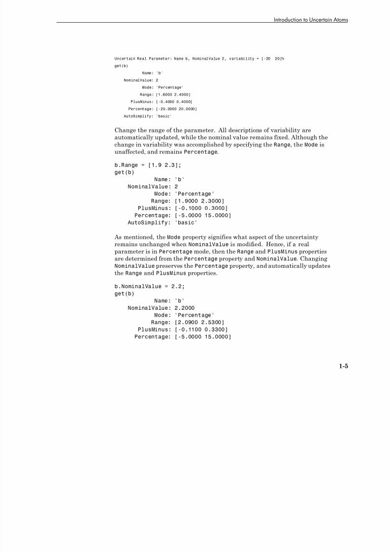
Uncertain Real Parameter: Name b, NominalValue 2, variability = [-20 20]%get(b)
Name: 'b'
NominalValue: 2
Mode: 'Percentage'
Range: [1.6000 2.4000]
PlusMinus: [-0.4000 0.4000]
Percentage: [-20.0000 20.0000]
AutoSimplify: 'basic'
Change the range of the parameter. All descriptions of variability are
automatically updated, while the nominal value remains fixed. Although the
change in variability was accomplished by specifying the Range, the Mode is
unaffected, and remains Percentage.
b.Range = [1.9 2.3];
get(b)
Name: 'b'NominalValue: 2
Mode: 'Percentage'
Range: [1.9000 2.3000]
PlusMinus: [-0.1000 0.3000]
Percentage: [-5.0000 15.0000]
AutoSimplify: 'basic'
As mentioned, the Mode property signifies what aspect of the uncertaintyremains unchanged when NominalValue is modified. Hence, if a real
parameter is in Percentage mode, then the Range and PlusMinus properties
are determined from the Percentage property and NominalValue. Changing
NominalValue preserves the Percentage property, and automatically updates
the Range and PlusMinus properties.
b.NominalValue = 2.2;
get(b)Name: 'b'
NominalValue: 2.2000
Mode: 'Percentage'
Range: [2.0900 2.5300]
PlusMinus: [-0.1100 0.3300]
Percentage: [-5.0000 15.0000]
1-5
7/30/2019 Robust Control Toolbox User's Guide
http://slidepdf.com/reader/full/robust-control-toolbox-users-guide 16/180
1 Building Uncertain Models
AutoSimplify: 'basic'
Create an uncertain parameter with an unsymmetric variation about its
nominal value.
c = ureal('c',-5,'per',[-20 30]);
get(c)
Name: 'c'
NominalValue: -5
Mode: 'Percentage'
Range: [-6 -3.5000]
PlusMinus: [-1 1.5000]
Percentage: [-20 30]
AutoSimplify: 'basic'
Create an uncertain parameter, specifying variability with Percentage, but
force the Mode to be Range.
d = ureal('d',-1,'mode','range','perc',[-40 60]);
get(d)
Name: 'd'
NominalValue: -1
Mode: 'Range'
Range: [-1.4000 -0.4000]
PlusMinus: [-0.4000 0.6000]
Percentage: [-40.0000 60] AutoSimplify: 'basic'
Finally, create an uncertain real parameter, and set the AutoSimplify
property to 'full'.
e = ureal('e',10,'plusminus',[-23],'mode','perce',...
'autosimplify','full')
Uncertain Real Parameter: Name e, NominalValue 10, variability = [-20 30]%
get(e)
Name: 'e'
NominalValue: 10
Mode: 'Percentage'
Range: [8 13]
PlusMinus: [-2 3]
1-6

7/30/2019 Robust Control Toolbox User's Guide
http://slidepdf.com/reader/full/robust-control-toolbox-users-guide 17/180
Introduction to Uncertain Atoms
Percentage: [-20 30]
AutoSimplify: 'full'
Specifying conflicting values for Range/Percentage/PlusMinus in a multiple
property/value set is not an error. In this case, the last (in list) specified
property is used. This last occurrence also determines the Mode, unless
Mode is explicitly specified, in which case that is used, regardless of the
property/value pairs ordering.
f = ureal('f',3,'plusminus',[-2 1],'perce',40)
Uncertain Real Parameter: Name f, NominalValue 3, variability = [-40 40]%
g = ureal('g',2,'plusminus',[-2 1],'mode','range','perce',40)
Uncertain Real Parameter: Name g, NominalValue 2, Range [1.2 2.8]
g.Mode
ans =
Range
Create an uncertain real parameter, use usample to generate 1000 instances(resulting in a 1-by-1-by-1000 array), reshape the array, and plot a histogram,
with 20 bins (within the range of 2 to 4).
h = ureal('h',3);
hsample = usample(h,1000);
hist(reshape(hsample,[1000 1]),20);
1-7
1

7/30/2019 Robust Control Toolbox User's Guide
http://slidepdf.com/reader/full/robust-control-toolbox-users-guide 18/180
1 Building Uncertain Models
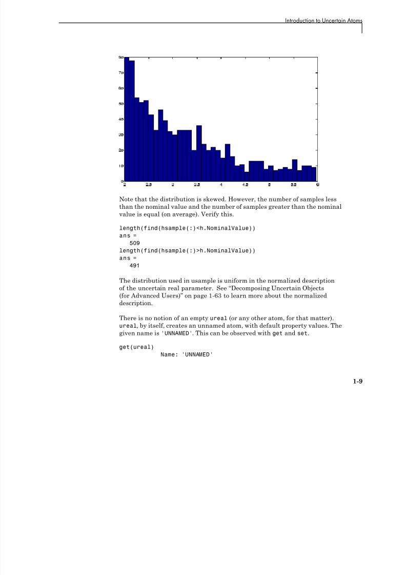
Make the range unsymmetric about the nominal value, and repeat the
sampling, and histogram plot (with 40 bins over the range of 2-to-6)
h.Range = [2 6];
hsample = usample(h,1000);
hist(reshape(hsample,[1000 1]),40);
1-8
7/30/2019 Robust Control Toolbox User's Guide
http://slidepdf.com/reader/full/robust-control-toolbox-users-guide 19/180
Introduction to Uncertain Atoms
Note that the distribution is skewed. However, the number of samples less
than the nominal value and the number of samples greater than the nominal
value is equal (on average). Verify this.
length(find(hsample(:)<h.NominalValue))
ans =
509
length(find(hsample(:)>h.NominalValue))
ans =
491
The distribution used in usample is uniform in the normalized description
of the uncertain real parameter. See “Decomposing Uncertain Objects
(for Advanced Users)” on page 1-63 to learn more about the normalized
description.
There is no notion of an empty ureal (or any other atom, for that matter).
ureal, by itself, creates an unnamed atom, with default property values. The
given name is 'UNNAMED'. This can be observed with get and set.
get(ureal)
Name: 'UNNAMED'
1-9
1 B ld U M d l

7/30/2019 Robust Control Toolbox User's Guide
http://slidepdf.com/reader/full/robust-control-toolbox-users-guide 20/180
1 Building Uncertain Models
NominalValue: 0
Mode: 'PlusMinus'
Range: [-1 1]
PlusMinus: [-1 1]
Percentage: [-Inf Inf]
AutoSimplify: 'basic'
set(ureal)
Name: 'String'
NominalValue: '1x1 real DOUBLE'
Mode: 'Range | PlusMinus'
Range: '1x2 DOUBLE'
PlusMinus: '1x2 or scalar DOUBLE'
Percentage: 'Not settable since Nominal==0'
AutoSimplify: '['off' | 'basic' | 'full']'
Uncertain LTI Dynamics Atoms
Uncertain linear, time-invariant objects, ultidyn, are used to representunknown linear, time-invariant dynamic objects, whose only known attributes
are bounds on their frequency response. Uncertain linear, time-invariant
objects have an internal name (the Name property), and are created by
specifying their size (number of outputs and number of inputs).
The property Type specifies whether the known attributes about the
frequency response are related to gain or phase. The property Type may be
'GainBounded' or 'PositiveReal'. The default value is 'GainBounded'.
The property Bound is a single number, which along with Type, completely
specifies what is known about the uncertain frequency response. Specifically,
if Δ is an ultidyn atom, and if γ denotes the value of the Bound property, then
the atom represents the set of all stable, linear, time-invariant systems whose
frequency response satisfies certain conditions:
If Type is 'GainBounded', Δ ( )⎡⎣ ⎤⎦ ≤ for all frequencies. When Type is'GainBounded', the default value for Bound (i.e., γ) is 1. The NominalValue
of Δ is always the 0-matrix.
If Type is 'PositiveReal', Δ(ω) + Δ*(ω) ≥ 2γ· for all frequencies. When Type is
'PositiveReal', the default value for Bound (i.e., γ) is 0. The NominalValue
is always (γ + 1 +2|γ|)I .
1-10
I t d ti t U t i At

7/30/2019 Robust Control Toolbox User's Guide
http://slidepdf.com/reader/full/robust-control-toolbox-users-guide 21/180
Introduction to Uncertain Atoms
All properties of a ultidyn are can be accessed with get and set (although
the NominalValue is determined from Type and Bound, and not accessible
with set). The properties are
Properties Meaning Class
Name Internal Name char
NominalValue Nominal value of atom See above
Type 'GainBounded' |'PositiveReal' charBound Norm bound or minimum real scalar double
SampleStateDim State-space dimension of random
samples of this uncertain element
scalar double
AutoSimplify 'off' | {'basic'} |'full' char
The SampleStateDim property specifies the state dimension of random
samples of the atom when using usample. The default value is 1. The AutoSimplify property serves the same function as in the uncertain real
parameter.
You can create a 2-by-3 gain-bounded uncertain linear dynamics atom. Verify
its size, and check the properties.
f = ultidyn('f',[2 3]);
size(f)ans =
2 3
get(f)
Name: 'f'
NominalValue: [2x3 double]
Type: 'GainBounded'
Bound: 1
SampleStateDim: 1 AutoSimplify: 'basic'
You can create a 1-by-1 (scalar) positive-real uncertain linear dynamics atom,
whose frequency response always has real part greater than -0.5. Set theSampleStateDim property to 5. View the properties, and plot a Nyquist plot
of 30 instances of the atom.
1-11
1 Building Uncertain Models

7/30/2019 Robust Control Toolbox User's Guide
http://slidepdf.com/reader/full/robust-control-toolbox-users-guide 22/180
1 Building Uncertain Models
g = ultidyn('g',[1 1],'type','positivereal','bound',-0.5);
g.SampleStateDim = 5;
get(g)
Name: 'g'
NominalValue: 1.5000
Type: 'PositiveReal'
Bound: -0.5000
SampleStateDim: 5
AutoSimplify: 'basic'
nyquist(usample(g,30))
xlim([-2 10])
ylim([-6 6]);
Time-Domain of ultidyn AtomsOn its own, every ultidyn atom is interpreted as a continuous-time, system
with uncertain behavior, quantified by bounds (gain or real-part) on its
frequency response. To see this, create a ultidyn, and view the sample time
of several random samples of the atom.
1-12
Introduction to Uncertain Atoms

7/30/2019 Robust Control Toolbox User's Guide
http://slidepdf.com/reader/full/robust-control-toolbox-users-guide 23/180
Introduction to Uncertain Atoms
h = ultidyn('h',[1 1]);
get(usample(h),'Ts')
ans =
0
get(usample(h),'Ts')
ans =
0
get(usample(h),'Ts')
ans =
0
However, when a ultidyn atom is an uncertain element of an uncertain
state space model (uss), then the time-domain characteristic of the atom is
determined from the time-domain characteristic of the system. The bounds
(gain-bounded or positivity) apply to the frequency-response of the atom.
This is explained and demonstrated in “Interpreting Uncertainty in Discrete
Time” on page 1-31.
Complex Parameter AtomsThe ucomplex atom represents an uncertain complex number, whose value
lies in a disc, centered at NominalValue, with radius specified by the Radius
property. The size of the disc can also be specified by Percentage, which
means the radius is derived from the absolute value of the NominalValue. The
properties of ucomplex objects are
Properties Meaning Class
Name Internal Name char
NominalValue Nominal value of atom double
Mode 'Range' | 'Percentage' char
Radius Radius of disk double
Percentage Additive variation (percent of Radius)
double
AutoSimplify 'off' | {'basic'} | 'full' char
The simplest construction requires only a name and nominal value. The
default Mode is Radius, and the default radius is 1.
1-13
1 Building Uncertain Models
7/30/2019 Robust Control Toolbox User's Guide
http://slidepdf.com/reader/full/robust-control-toolbox-users-guide 24/180
1 Building Uncertain Models
a = ucomplex('a',2-j)
Uncertain Complex Parameter: Name a, NominalValue 2-1i, Radius 1
get(a)
Name: 'a'
NominalValue: 2.0000- 1.0000i
Mode: 'Radius'
Radius: 1
Percentage: 44.7214
AutoSimplify: 'basic'
set(a)Name: 'String'
NominalValue: '1x1 DOUBLE'
Mode: 'Radius | Percentage'
Radius: 'scalar DOUBLE'
Percentage: 'scalar DOUBLE'
AutoSimplify: '['off' | 'basic' | 'full']'
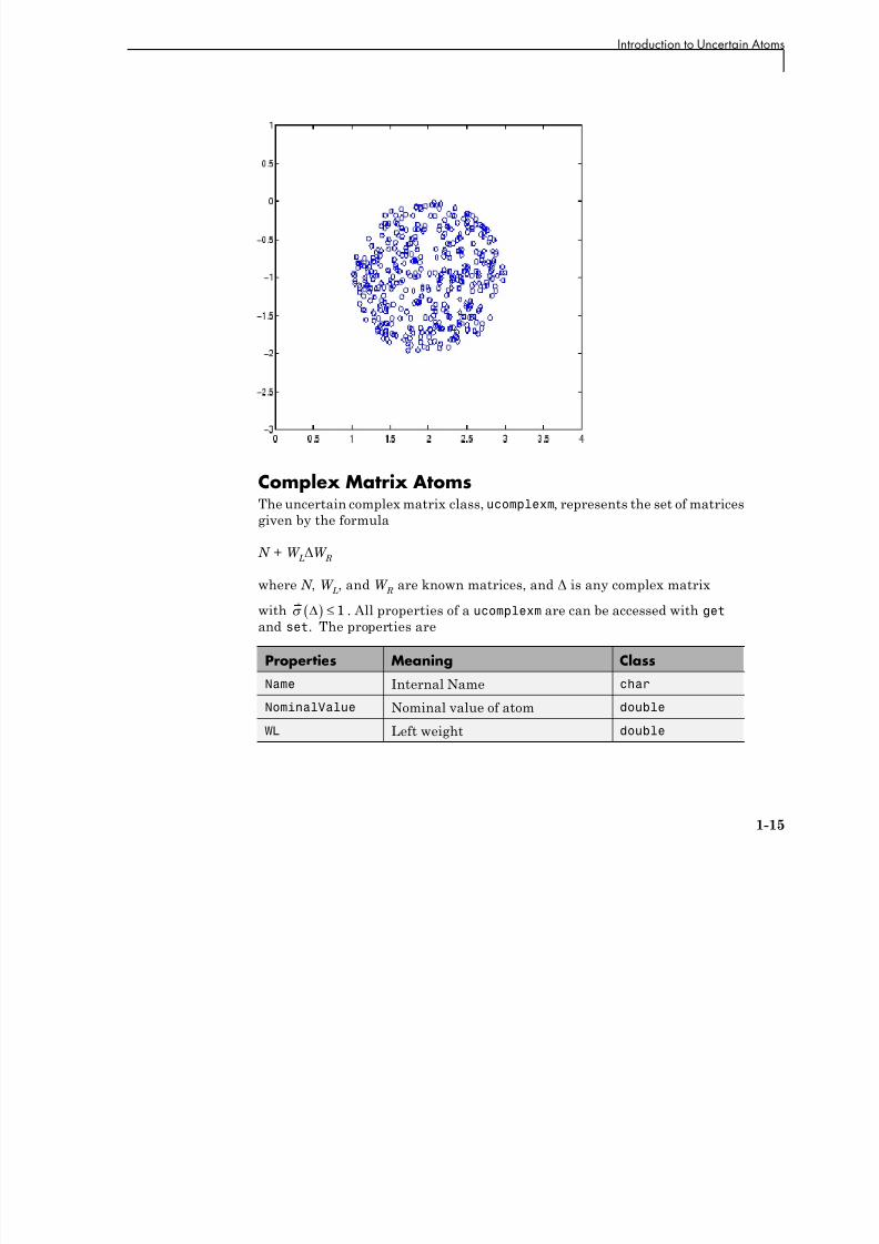
Sample the uncertain complex parameter at 400 values, and plot in thecomplex plane. Clearly, the samples appear to be from a disc of radius 1,
centered in the complex plane at the value 2- j.
asample = usample(a,400);
plot(asample(:),'o'); xlim([0 4]); ylim([-3 1]);
1-14
Introduction to Uncertain Atoms
7/30/2019 Robust Control Toolbox User's Guide
http://slidepdf.com/reader/full/robust-control-toolbox-users-guide 25/180
Complex Matrix AtomsThe uncertain complex matrix class, ucomplexm, represents the set of matrices
given by the formula
N + W L ΔW
R
where N , W L
, and W R
are known matrices, and Δ is any complex matrix
with Δ( ) ≤ 1 . All properties of a ucomplexm are can be accessed with get
and set. The properties are
Properties Meaning Class
Name Internal Name char
NominalValue Nominal value of atom double
WL Left weight double
1-15
1 Building Uncertain Models

7/30/2019 Robust Control Toolbox User's Guide
http://slidepdf.com/reader/full/robust-control-toolbox-users-guide 26/180
Properties Meaning Class WR Right weight double
AutoSimplify 'off' | {'basic'} | 'full' char
The simplest construction requires only a name and nominal value. The
default left and right weight matrices are identity.
You can create a 4-by-3 ucomplexm element, and view its properties.
m = ucomplexm('m',[1 2 3;4 5 6;7 8 9;10 11 12])
Uncertain Complex Matrix: Name m, 4x3
get(m)
Name: 'm'
NominalValue: [4x3 double]
WL: [4x4 double]
WR: [3x3 double]
AutoSimplify: 'basic'
m.NominalValue
ans =
1 2 3
4 5 6
7 8 9
10 11 12
m.WL
ans =
1 0 0 0
0 1 0 0
0 0 1 0
0 0 0 1
Sample the uncertain matrix, and compare to the nominal value. Note the
element-by-element sizes of the difference are generally equal, indicative of
the default (identity) weighting matrices that are in place.
abs(usample(m)-m.NominalValue)
ans =
0.2948 0.1001 0.2867
0.3028 0.2384 0.2508
0.3376 0.1260 0.2506
1-16
Introduction to Uncertain Atoms
7/30/2019 Robust Control Toolbox User's Guide
http://slidepdf.com/reader/full/robust-control-toolbox-users-guide 27/180
0.2200 0.3472 0.1657
Change the left and right weighting matrices, making the uncertainty larger
as you move down the rows, and across the columns.
m.WL = diag([0.2 0.4 0.8 1.6]);
m.WR = diag([0.1 1 4]);
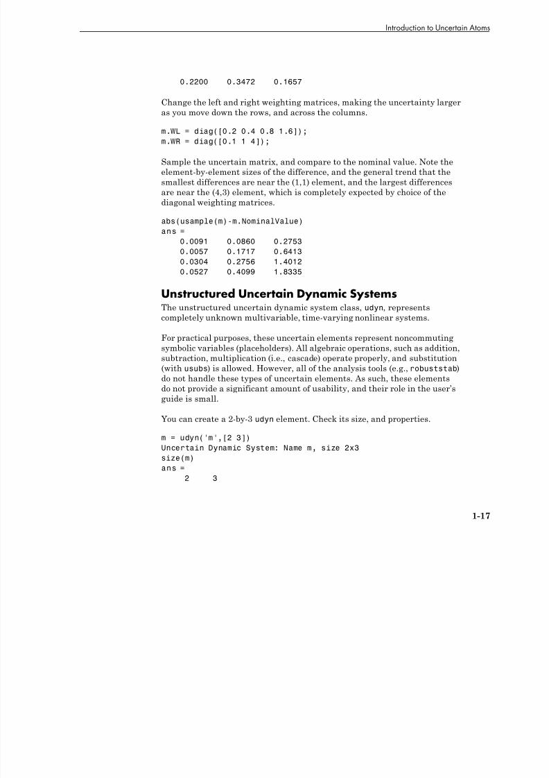
Sample the uncertain matrix, and compare to the nominal value. Note the
element-by-element sizes of the difference, and the general trend that thesmallest differences are near the (1,1) element, and the largest differences
are near the (4,3) element, which is completely expected by choice of the
diagonal weighting matrices.
abs(usample(m)-m.NominalValue)
ans =
0.0091 0.0860 0.2753
0.0057 0.1717 0.64130.0304 0.2756 1.4012
0.0527 0.4099 1.8335
Unstructured Uncertain Dynamic SystemsThe unstructured uncertain dynamic system class, udyn, represents
completely unknown multivariable, time-varying nonlinear systems.
For practical purposes, these uncertain elements represent noncommutingsymbolic variables (placeholders). All algebraic operations, such as addition,
subtraction, multiplication (i.e., cascade) operate properly, and substitution
(with usubs) is allowed. However, all of the analysis tools (e.g., robuststab)
do not handle these types of uncertain elements. As such, these elements
do not provide a significant amount of usability, and their role in the user’s
guide is small.
You can create a 2-by-3 udyn element. Check its size, and properties.
m = udyn('m',[2 3])
Uncertain Dynamic System: Name m, size 2x3
size(m)
ans =
2 3
1-17
1 Building Uncertain Models

7/30/2019 Robust Control Toolbox User's Guide
http://slidepdf.com/reader/full/robust-control-toolbox-users-guide 28/180
get(m)
Name: 'm'
NominalValue: [2x3 double]
AutoSimplify: 'basic'
1-18
Uncertain Matrices

7/30/2019 Robust Control Toolbox User's Guide
http://slidepdf.com/reader/full/robust-control-toolbox-users-guide 29/180
Uncertain MatricesUncertain matrices (class umat) are built from doubles, and uncertain atoms,
using traditional MATLAB matrix building syntax. Uncertain matrices
can be added, subtracted, multiplied, inverted, transposed, etc., resulting
in uncertain matrices. The rows and columns of an uncertain matrix are
referenced in the same manner that MATLAB references rows and columns
of an array, using parenthesis, and integer indices. The NominalValue of a
uncertain matrix is the result obtained when all uncertain atoms are replaced
with their own NominalValue. The uncertain atoms making up a umat are
accessible through the Uncertainty gateway, and the properties of each atom
within a umat can be changed directly.
Using usubs, specific values may be substituted for any of the uncertain
atoms within a umat. The command usample generates a random sample of
the uncertain matrix, substituting random samples (within their ranges) for
each of the uncertain atoms.
The command wcnorm computes tight bounds on the worst-case (maximum
over the uncertain elements’ ranges) norm of the uncertain matrix.
Standard MATLAB numerical matrices (i.e., double) naturally can be viewed
as uncertain matrices without any uncertainty.
Creating Uncertain Matrices from Uncertain Atoms You can create 2 uncertain real parameters, and then a 3-by-2 uncertain
matrix using these uncertain atoms.
a = ureal('a',3);
b = ureal('b',10,'pe',20);
M = [-a 1/b;b a+1/b;1 3]
UMAT: 3 Rows, 2 Columns
a: real, nominal = 3, variability = [-1 1], 2 occurrencesb: real, nominal = 10, variability = [-20 20]%, 3 occurrences
The size and class of M are as expected
size(M)
ans =
1-19
1 Building Uncertain Models

7/30/2019 Robust Control Toolbox User's Guide
http://slidepdf.com/reader/full/robust-control-toolbox-users-guide 30/180
3 2
class(M)
ans =
umat
Accessing Properties of a umatUse get to view the accessible properties of a umat.
get(M)
NominalValue: [3x2 double]
Uncertainty: [1x1 atomlist]
The NominalValue is a double, obtained by replacing all uncertain elements
with their nominal values.
M.NominalValue
ans =
-3.0000 0.100010.0000 3.1000
1.0000 3.0000
The Uncertainty property is a atomlist object, which is simply a gateway
from the umat to the uncertain atoms.
class(M.Uncertainty)
ans =atomlist
M.Uncertainty
a: [1x1 ureal]
b: [1x1 ureal]
Direct access to the atoms is facilitated through Uncertainty. Check the
Range of the uncertain element named 'a' within M, then change it.
M.Uncertainty.a.Range
ans =
2 4
M.Uncertainty.a.Range = [2.5 5];
M
UMAT: 3 Rows, 2 Columns
1-20
Uncertain Matrices

7/30/2019 Robust Control Toolbox User's Guide
http://slidepdf.com/reader/full/robust-control-toolbox-users-guide 31/180
a: real, nominal = 3, variability = [-0.5 2], 2 occurrences
b: real, nominal = 10, variability = [-20 20]%, 3 occurrences
The change to the uncertain real parameter a only took place within M. Verify
that the variable a in the workspace is no longer the same as the variable a
within M.
isequal(M.Uncertainty.a,a)
ans =
0
Note that combining atoms which have a common internal name, but different
properties leads to an error. For instance, subtracting the two atoms gives
an error, not 0.
M.Uncertainty.a - a
??? Error using ==> ndlft.lftmask
Atoms named 'a' have different properties.
Row and Column ReferencingStandard Row/Column referencing is allowed. Note, however, that
single-indexing is only allowed if the umat is a column or a row.
Reconstruct M (if need be), and make a 2-by-2 selection from M
a = ureal('a',3);
b = ureal('b',10,'pe',20);
M = [-a 1/b;b a+1/b;1 3];
M.Uncertainty.a.Range = [2.5 5];
M(2:3,:)
UMAT: 2 Rows, 2 Columns
a: real, nominal = 3, variability = [-0.5 2], 1 occurrence
b: real, nominal = 10, variability = [-20 20]%, 2 occurrences
Make a single column selection from M, and use single-index references to
access elements of it.
h = M([2 1 2 3],2)
UMAT: 4 Rows, 1 Columns
1-21
1 Building Uncertain Models
7/30/2019 Robust Control Toolbox User's Guide
http://slidepdf.com/reader/full/robust-control-toolbox-users-guide 32/180
a: real, nominal = 3, variability = [-0.5 2], 1 occurrence
b: real, nominal = 10, variability = [-20 20]%, 1 occurrenceh(2)
UMAT: 1 Rows, 1 Columns
b: real, nominal = 10, variability = [-20 20]%, 1 occurrence
h(3)
UMAT: 1 Rows, 1 Columns
a: real, nominal = 3, variability = [-0.5 2], 1 occurrence
b: real, nominal = 10, variability = [-20 20]%, 1 occurrence
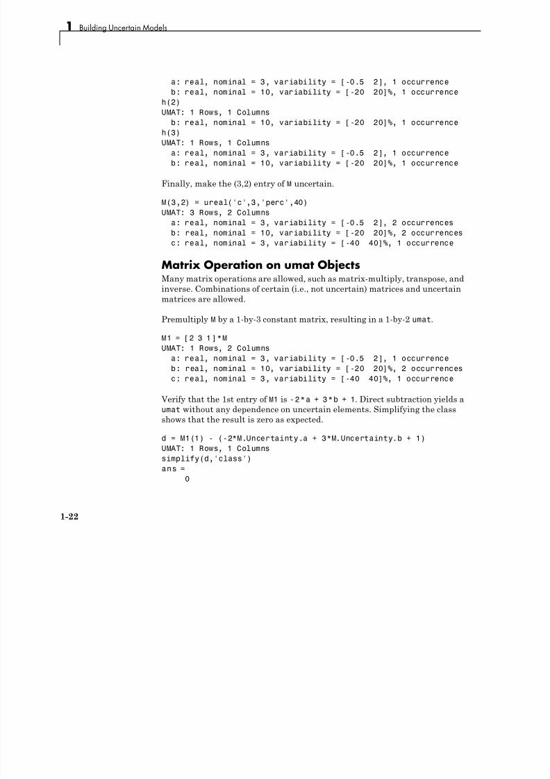
Finally, make the (3,2) entry of M uncertain.
M(3,2) = ureal('c',3,'perc',40)
UMAT: 3 Rows, 2 Columns
a: real, nominal = 3, variability = [-0.5 2], 2 occurrences
b: real, nominal = 10, variability = [-20 20]%, 2 occurrences
c: real, nominal = 3, variability = [-40 40]%, 1 occurrence
Matrix Operation on umat ObjectsMany matrix operations are allowed, such as matrix-multiply, transpose, and
inverse. Combinations of certain (i.e., not uncertain) matrices and uncertain
matrices are allowed.
Premultiply M by a 1-by-3 constant matrix, resulting in a 1-by-2 umat.
M1 = [2 3 1]*MUMAT: 1 Rows, 2 Columns
a: real, nominal = 3, variability = [-0.5 2], 1 occurrence
b: real, nominal = 10, variability = [-20 20]%, 2 occurrences
c: real, nominal = 3, variability = [-40 40]%, 1 occurrence
Verify that the 1st entry of M1 is -2*a + 3*b + 1. Direct subtraction yields a
umat without any dependence on uncertain elements. Simplifying the class
shows that the result is zero as expected.
d = M1(1) - (-2*M.Uncertainty.a + 3*M.Uncertainty.b + 1)
UMAT: 1 Rows, 1 Columns
simplify(d,'class')
ans =
0
1-22
Uncertain Matrices

7/30/2019 Robust Control Toolbox User's Guide
http://slidepdf.com/reader/full/robust-control-toolbox-users-guide 33/180
Transpose M, form a product, an inverse, and sample the uncertain result. Asexpected, the result is the 2-by-2 identity matrix.
H = M.'*M;
K = inv(H);
usample(K*H,3)
ans(:,:,1) =
1.0000 -0.0000
-0.0000 1.0000ans(:,:,2) =
1.0000 -0.0000
-0.0000 1.0000
ans(:,:,3) =
1.0000 -0.0000
-0.0000 1.0000
Substituting for Uncertain AtomsUncertain atoms can be substituted for using usubs. For more information,
see “Substitution by usubs” on page 1-49. Here, we illustrate a few special
cases.
Substitute all instances of the uncertain real parameter named a with the
number 4. This results in a umat, with dependence on the uncertain real
parameters b and c.
M2 = usubs(M,'a',4)
UMAT: 3 Rows, 2 Columns
b: real, nominal = 10, variability = [-20 20]%, 2 occurrences
c: real, nominal = 3, variability = [-40 40]%, 1 occurrence
Similarly, we can substitute all instances of the uncertain real parameter
named b with M.Uncertainty.a, resulting in a umat with dependence on the
uncertain real parameters a and c.
M3 = usubs(M,'b', M.Uncertainty.a)
UMAT: 3 Rows, 2 Columns
a: real, nominal = 3, variability = [-0.5 2], 4 occurrences
c: real, nominal = 3, variability = [-40 40]%, 1 occurrence
Nominal and/or random instances can easily be specified.
1-23
1 Building Uncertain Models
7/30/2019 Robust Control Toolbox User's Guide
http://slidepdf.com/reader/full/robust-control-toolbox-users-guide 34/180
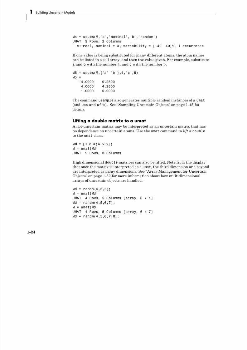
M4 = usubs(M,'a','nominal','b','random')
UMAT: 3 Rows, 2 Columnsc: real, nominal = 3, variability = [-40 40]%, 1 occurrence
If one value is being substituted for many different atoms, the atom names
can be listed in a cell array, and then the value given. For example, substitute
a and b with the number 4, and c with the number 5.
M5 = usubs(M,{'a' 'b'},4,'c',5)
M5 =-4.0000 0.2500
4.0000 4.2500
1.0000 5.0000
The command usample also generates multiple random instances of a umat
(and uss and ufrd). See “Sampling Uncertain Objects” on page 1-45 for
details.
Lifting a double matrix to a umat A not-uncertain matrix may be interpreted as an uncertain matrix that has
no dependence on uncertain atoms. Use the umat command to lift a double
to the umat class.
M d = [ 1 2 3 ; 4 5 6 ] ;
M = umat(Md)
UMAT: 2 Rows, 3 Columns
High dimensional double matrices can also be lifted. Note from the display
that once the matrix is interpreted as a umat, the third dimension and beyond
are interpreted as array dimensions. See “Array Management for UncertainObjects” on page 1-52 for more information about how multidimensional
arrays of uncertain objects are handled.
Md = randn(4,5,6);M = umat(Md)
UMAT: 4 Rows, 5 Columns [array, 6 x 1]
Md = randn(4,5,6,7);
M = umat(Md)
UMAT: 4 Rows, 5 Columns [array, 6 x 7]
Md = randn(4,5,6,7,8);
1-24
Uncertain Matrices

7/30/2019 Robust Control Toolbox User's Guide
http://slidepdf.com/reader/full/robust-control-toolbox-users-guide 35/180
M = umat(Md)
UMAT: 4 Rows, 5 Columns [array, 6 x 7 x 8]
1-25
1 Building Uncertain Models
7/30/2019 Robust Control Toolbox User's Guide
http://slidepdf.com/reader/full/robust-control-toolbox-users-guide 36/180
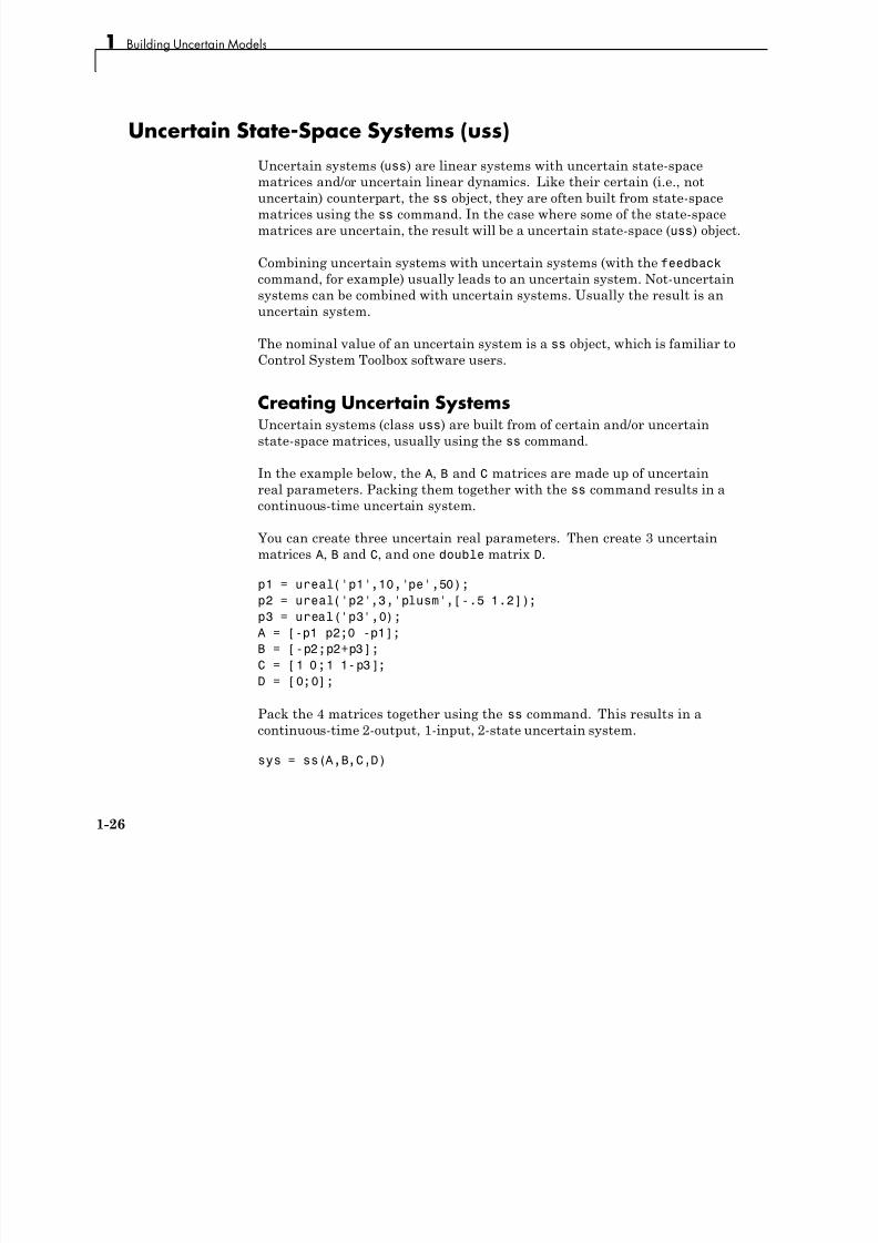
Uncertain State-Space Systems (uss)
Uncertain systems (uss) are linear systems with uncertain state-space
matrices and/or uncertain linear dynamics. Like their certain (i.e., not
uncertain) counterpart, the ss object, they are often built from state-space
matrices using the ss command. In the case where some of the state-space
matrices are uncertain, the result will be a uncertain state-space (uss) object.
Combining uncertain systems with uncertain systems (with the feedback
command, for example) usually leads to an uncertain system. Not-uncertainsystems can be combined with uncertain systems. Usually the result is an
uncertain system.
The nominal value of an uncertain system is a ss object, which is familiar to
Control System Toolbox software users.
Creating Uncertain SystemsUncertain systems (class uss) are built from of certain and/or uncertain
state-space matrices, usually using the ss command.
In the example below, the A, B and C matrices are made up of uncertain
real parameters. Packing them together with the ss command results in a
continuous-time uncertain system.
You can create three uncertain real parameters. Then create 3 uncertainmatrices A, B and C, and one double matrix D.
p1 = ureal('p1',10,'pe',50);
p2 = ureal('p2',3,'plusm',[-.5 1.2]);
p3 = ureal('p3',0);
A = [-p1 p2;0 -p1];
B = [-p2;p2+p3];
C = [1 0;1 1-p3];
D = [0;0];
Pack the 4 matrices together using the ss command. This results in a
continuous-time 2-output, 1-input, 2-state uncertain system.
sys = ss(A,B,C,D)
1-26
Uncertain State-Space Systems (uss)
7/30/2019 Robust Control Toolbox User's Guide
http://slidepdf.com/reader/full/robust-control-toolbox-users-guide 37/180
USS: 2 States, 2 Outputs, 1 Input, Continuous System
p1: real, nominal = 10, variability = [-50 50]%, 2 occurrencesp2: real, nominal = 3, variability = [-0.5 1.2], 2 occurrences
p3: real, nominal = 0, variability = [-1 1], 2 occurrences
Properties of uss Objects View the properties with the get command.
get(sys)
a: [2x2 umat]
b: [2x1 umat]
c: [2x2 umat]
d: [2x1 double]
StateName: {2x1 cell}
Ts: 0
InputName: {''}
OutputName: {2x1 cell}
InputGroup: [1x1 struct]OutputGroup: [1x1 struct]
NominalValue: [2x1 ss]
Uncertainty: [1x1 atomlist]
Notes: {}
UserData: []
The properties a , b , c , d, and StateName behave in exactly the same
manner as Control System Toolbox ss objects. The properties InputName,OutputName, InputGroup and OutputGroup behave in exactly the same
manner as all of the Control System Toolbox system objects ( ss, zpk, tf,
and frd).
The NominalValue is a Control System Toolbox ss object, and hence all
methods for ss objects are available. For instance, compute the poles and
step response of the nominal system.
pole(sys.NominalValue)
ans =
-10
-10
step(sys.NominalValue)
1-27
1 Building Uncertain Models

7/30/2019 Robust Control Toolbox User's Guide
http://slidepdf.com/reader/full/robust-control-toolbox-users-guide 38/180
Just as with the umat class, the Uncertainty property is a atomlist object,
acting as a gateway to the uncertain atoms. Direct access to the atoms is
facilitated through Uncertainty. Check the Range of the uncertain element
named 'p2' within sys, then change its left endpoint.
sys.Uncertainty.p2.range
ans =
2.5000 4.2000
sys.Uncertainty.p2.range(1) = 2;
Sampling Uncertain SystemsThe command usample randomly samples the uncertain system at a specified
number of points.
Randomly sample the uncertain system at 20 points in its modeled
uncertainty range. This gives a 20-by-1 ss array. Consequently, all analysistools from Control System Toolbox software are available.
manysys = usample(sys,20);
size(manysys)
20x1 array of state-space models
Each model has 2 outputs, 1 input, and 2 states.
1-28
Uncertain State-Space Systems (uss)
7/30/2019 Robust Control Toolbox User's Guide
http://slidepdf.com/reader/full/robust-control-toolbox-users-guide 39/180
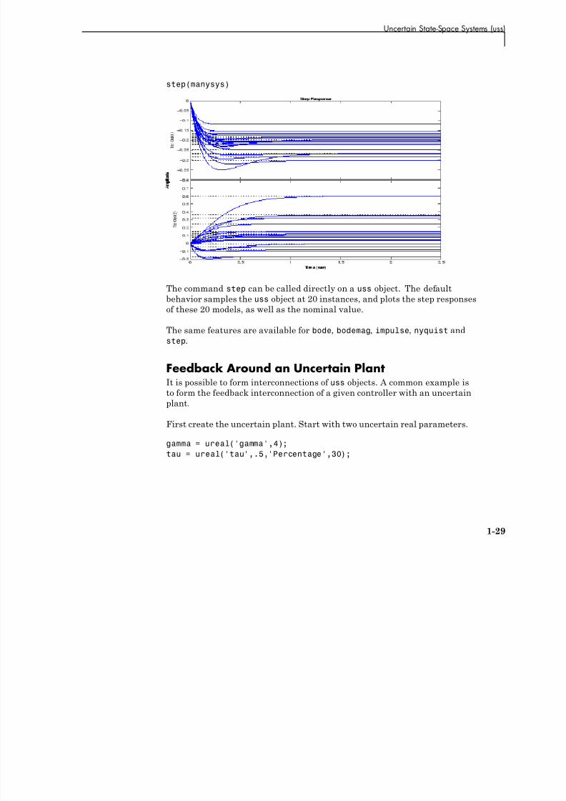
step(manysys)
The command step can be called directly on a uss object. The default
behavior samples the uss object at 20 instances, and plots the step responses
of these 20 models, as well as the nominal value.
The same features are available for bode, bodemag, impulse, nyquist and
step.
Feedback Around an Uncertain PlantIt is possible to form interconnections of uss objects. A common example is
to form the feedback interconnection of a given controller with an uncertain
plant.
First create the uncertain plant. Start with two uncertain real parameters.
gamma = ureal('gamma',4);
tau = ureal('tau',.5,'Percentage',30);
1-29
1 Building Uncertain Models

7/30/2019 Robust Control Toolbox User's Guide
http://slidepdf.com/reader/full/robust-control-toolbox-users-guide 40/180
Next, create an unmodeled dynamics atom, delta, and a 1st order weighting
function, whose DC value is 0.2, high-frequency gain is 10, and whosecrossover frequency is 8 rad/sec.
delta = ultidyn('delta',[1 1],'SampleStateDim',5);
W = makeweight(0.2,6,6);
Finally, create the uncertain plant consisting of the uncertain parameters
and the unmodeled dynamics.
P = tf(gamma,[tau 1])*(1+W*delta);
You can create an integral controller based on nominal plant parameters.
Nominally the closed-loop system will have damping ratio of 0.707 and time
constant of 2*tau.
KI = 1/(2*tau.Nominal*gamma.Nominal);
C = tf(KI,[1 0]);
Create the uncertain closed-loop system using the feedback command.
CLP = feedback(P*C,1);
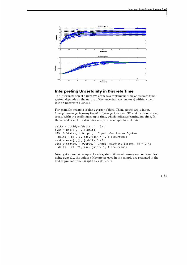
Using usample and step, plot samples of the open-loop and closed-loop step
responses. As expected the integral controller reduces the variability in the
low frequency response.
subplot(2,1,1); step(P,5,20)
subplot(2,1,2); step(CLP,5,20)
1-30
Uncertain State-Space Systems (uss)
7/30/2019 Robust Control Toolbox User's Guide
http://slidepdf.com/reader/full/robust-control-toolbox-users-guide 41/180
Interpreting Uncertainty in Discrete TimeThe interpretation of a ultidyn atom as a continuous-time or discrete-time
system depends on the nature of the uncertain system (uss) within which
it is an uncertain element.
For example, create a scalar ultidyn object. Then, create two 1-input,
1-output uss objects using the ultidyn object as their “D” matrix. In one case,
create without specifying sample-time, which indicates continuous time. Inthe second case, force discrete-time, with a sample time of 0.42.
delta = ultidyn('delta',[1 1]);
sys1 = uss([],[],[],delta)
USS: 0 States, 1 Output, 1 Input, Continuous System
delta: 1x1 LTI, max. gain = 1, 1 occurrence
sys2 = uss([],[],[],delta,0.42)
USS: 0 States, 1 Output, 1 Input, Discrete System, Ts = 0.42delta: 1x1 LTI, max. gain = 1, 1 occurrence
Next, get a random sample of each system. When obtaining random samples
using usample, the values of the atoms used in the sample are returned in the
2nd argument from usample as a structure.
1-31
1 Building Uncertain Models

7/30/2019 Robust Control Toolbox User's Guide
http://slidepdf.com/reader/full/robust-control-toolbox-users-guide 42/180
[sys1s,d1v] = usample(sys1);
[sys2s,d2v] = usample(sys2);
Look at d1v.delta.Ts and d2v.delta.Ts. In the first case, since sys1 is
continuous-time, the system d1v.delta is continuous-time. In the second
case, since sys2 is discrete-time, with sample time 0.42, the system d2v.delta
is discrete-time, with sample time 0.42.
d1v.delta.Ts
ans =0
d2v.delta.Ts
ans =
0.4200
Finally, in the case of a discrete-time uss object, it is not the case thatultidyn objects are interpreted as continuous-time uncertainty in feedback
with sampled-data systems. This very interesting hybrid theory is beyond thescope of the toolbox.
Lifting a ss to a uss A not-uncertain state space object may be interpreted as an uncertain state
space object that has no dependence on uncertain atoms. Use the uss
command to “lift” a ss to the uss class.
sys = rss(3,2,1);
usys = uss(sys)
USS: 3 States, 2 Outputs, 1 Input, Continuous System
Arrays of ss objects can also be lifted. See “Array Management for Uncertain
Objects” on page 1-52 for more information about how arrays of uncertain
objects are handled.
Handling Delays in ussIn the current implementation, delays are not allowed. Delays are omitted
and a warning is displayed when ss objects are lifted to uss objects.
sys = rss(3,2,1);
1-32
Uncertain State-Space Systems (uss)
7/30/2019 Robust Control Toolbox User's Guide
http://slidepdf.com/reader/full/robust-control-toolbox-users-guide 43/180
sys.inputdelay = 1.3;
usys = uss(sys) Warning: Omitting DELAYs in conversion to USS
> In uss.uss at 103
USS: 3 States, 2 Outputs, 1 Input, Continuous System
This lifting process happens in the background whenever ss objects are
combined with any uncertain object. Consequently all delays will be lost in
such operations.
Use the command pade to approximately preserve the effect of the time delay
in the ss object. Before operations involving ss objects containing delays
and uncertain objects, use the pade command to convert the ss object to a
delay free object.
For example, consider an uncertain system with a time constant
approximately equal to 1, an extra input delay of 0.3 seconds, second-order
rolloff beyond 20 rad/s, and an uncertain steady-state gain ranging from 4 to6. This can be approximated using the pade command, as follows:
sys = tf(1,[1 1])*tf(1,[0.05 1]);
sys.inputdelay = 0.3;
gain = ureal('gain',5);
usys = gain*pade(sys,4)
USS: 6 States, 1 Output, 1 Input, Continuous System
gain: real, nominal = 5, variability = [-1 1], 1 occurrence
If gain is multiplied by sys directly, the time delay is unfortunately omitted,
since this operation involves lifting sys to a uss as described above. The
difference is obvious from the step responses.
step(usys,gain*sys,4,5)
Warning: Omitting DELAYs in conversion to USS
> In uss.uss at 103
In umat.umat at 98In atom.mtimes at 7
1-33
1 Building Uncertain Models

7/30/2019 Robust Control Toolbox User's Guide
http://slidepdf.com/reader/full/robust-control-toolbox-users-guide 44/180
1-34
Uncertain frd
7/30/2019 Robust Control Toolbox User's Guide
http://slidepdf.com/reader/full/robust-control-toolbox-users-guide 45/180
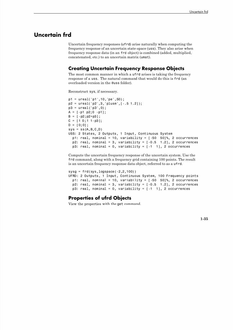
Uncertain frd
Uncertain frequency responses (ufrd) arise naturally when computing the
frequency response of an uncertain state-space (uss). They also arise when
frequency response data (in an frd object) is combined (added, multiplied,
concatenated, etc.) to an uncertain matrix (umat).
Creating Uncertain Frequency Response Objects
The most common manner in which a ufrd arises is taking the frequencyresponse of a uss. The natural command that would do this is frd (an
overloaded version in the @uss folder).
Reconstruct sys, if necessary.
p1 = ureal('p1',10,'pe',50);
p2 = ureal('p2',3,'plusm',[-.5 1.2]);
p3 = ureal('p3',0); A = [-p1 p2;0 -p1];
B = [-p2;p2+p3];
C = [1 0;1 1-p3];
D = [0;0];
sys = ss(A,B,C,D)
USS: 2 States, 2 Outputs, 1 Input, Continuous System
p1: real, nominal = 10, variability = [-50 50]%, 2 occurrences
p2: real, nominal = 3, variability = [-0.5 1.2], 2 occurrences
p3: real, nominal = 0, variability = [-1 1], 2 occurrences
Compute the uncertain frequency response of the uncertain system. Use thefrd command, along with a frequency grid containing 100 points. The resultis an uncertain frequency response data object, referred to as a ufrd.
sysg = frd(sys,logspace(-2,2,100))
UFRD: 2 Outputs, 1 Input, Continuous System, 100 Frequency points
p1: real, nominal = 10, variability = [-50 50]%, 2 occurrencesp2: real, nominal = 3, variability = [-0.5 1.2], 2 occurrences
p3: real, nominal = 0, variability = [-1 1], 2 occurrences
Properties of ufrd Objects View the properties with the get command.
1-35
1 Building Uncertain Models

7/30/2019 Robust Control Toolbox User's Guide
http://slidepdf.com/reader/full/robust-control-toolbox-users-guide 46/180
get(sysg)
Frequency: [100x1 double]ResponseData: [2x1x100 umat]
Units: 'rad/s'
Ts: 0
InputName: {''}
OutputName: {2x1 cell}
InputGroup: [1x1 struct]
OutputGroup: [1x1 struct]
NominalValue: [2x1 frd]Uncertainty: [1x1 atomlist]
Notes: {}
UserData: []
Version: 4
The properties ResponseData and Frequency behave in exactly the same
manner as Control System Toolbox frd objects, except that ResponseData
is a umat. The properties InputName, OutputName, InputGroup andOutputGroup behave in exactly the same manner as all of the Control System
Toolbox system objects (ss, zpk, tf, and frd).
The NominalValue is a Control System Toolbox frd object, and hence all
methods for frd objects are available. For instance, plot the Bode response of
the nominal system.
bode(sysg.nom)
1-36
Uncertain frd

7/30/2019 Robust Control Toolbox User's Guide
http://slidepdf.com/reader/full/robust-control-toolbox-users-guide 47/180
Just as with the umat and uss classes, the Uncertainty property is an
atomlist object, acting as a gateway to the uncertain atoms. Direct access to
the atoms is facilitated through Uncertainty. Change the nominal value of
the uncertain element named 'p1' within sysg to 14, and replot the Bode plot
of the (new) nominal system.
sysg.unc.p1.nom = 14
UFRD: 2 Outputs, 1 Input, Continuous System, 100 Frequency points
p1: real, nominal = 14, variability = [-50 50]%, 2 occurrences
p2: real, nominal = 3, variability = [-0.5 1.2], 2 occurrencesp3: real, nominal = 0, variability = [-1 1], 2 occurrences
Interpreting Uncertainty in Discrete TimeSee “Interpreting Uncertainty in Discrete Time” on page 1-31. The issues
are identical.
1-37
1 Building Uncertain Models

7/30/2019 Robust Control Toolbox User's Guide
http://slidepdf.com/reader/full/robust-control-toolbox-users-guide 48/180
Lifting an frd to a ufrd A not-uncertain frequency response object may be interpreted as an uncertainfrequency response object that has no dependence on uncertain atoms. Use
the ufrd command to “lift” an frd object to the ufrd class.
sys = rss(3,2,1);
sysg = frd(sys,logspace(-2,2,100));
usysg = ufrd(sysg)
UFRD: 2 Outputs, 1 Input, Continuous System, 100 Frequency points
Arrays of frd objects can also be lifted. See “Array Management for Uncertain
Objects” on page 1-52 for more information about how arrays of uncertain
objects are handled.
Handling Delays in ufrdSee “Handling Delays in uss” on page 1-32. The issues are identical.
1-38
Basic Control System Toolbox™ and MATLAB® Interconnections

7/30/2019 Robust Control Toolbox User's Guide
http://slidepdf.com/reader/full/robust-control-toolbox-users-guide 49/180
Basic Control System Toolbox and MATLAB Interconnections
This list has all of the basic system interconnection functions defined in
Control System Toolbox software or in MATLAB.
• append
• blkdiag
• series
• parallel
• feedback
• lft
• stack
These functions work with uncertain objects as well. Uncertain objects may
be combined with certain objects, resulting in an uncertain object.
1-39
1 Building Uncertain Models

7/30/2019 Robust Control Toolbox User's Guide
http://slidepdf.com/reader/full/robust-control-toolbox-users-guide 50/180
Simplifying Representation of Uncertain Objects
A minimal realization of the transfer function matrix
H ss s
s s
( ) = + +
+ +
⎡
⎣
⎢⎢⎢⎢
⎤
⎦
⎥⎥⎥⎥
2
1
4
1
3
1
6
1
has only 1 state, obvious from the decomposition
H ss
( ) =⎡
⎣⎢
⎤
⎦⎥ +
[ ]2
3
1
11 2 .
However, a “natural” construction, formed by
sys11 = ss(tf(2,[1 1]));sys12 = ss(tf(4,[1 1]));
sys21 = ss(tf(3,[1 1]));
sys22 = ss(tf(6,[1 1]));
sys = [sys11 sys12;sys21 sys22]
a =
x1 x2 x3 x4
x1 -1 0 0 0
x2 0 -1 0 0x3 0 0 -1 0
x4 0 0 0 -1
b =
u1 u2
x1 2 0
x2 0 2
x3 2 0
x4 0 2c =
x1 x2 x3 x4
y1 1 2 0 0
y2 0 0 1.5 3
d =
u1 u2
1-40
Simplifying Representation of Uncertain Objects

7/30/2019 Robust Control Toolbox User's Guide
http://slidepdf.com/reader/full/robust-control-toolbox-users-guide 51/180
y1 0 0
y2 0 0Continuous-time model
has four states, and is nonminimal.
In the same manner, the internal representation of uncertain objects built up
from uncertain atoms can become nonminimal, depending on the sequence
of operations in their construction. The command simplify employs
ad-hoc simplification and reduction schemes to reduce the complexity of therepresentation of uncertain objects. There are three levels of simplification:
off, basic and full. Each uncertain atom has an AutoSimplify property whose
value is one of the strings 'off', 'basic' or 'full'. The default value
is 'basic'.
After (nearly) every operation, the command simplify is automatically run
on the uncertain object, cycling through all of the uncertain atoms, and
attempting to simplify (without error) the representation of the effect of thatuncertain object. The AutoSimplify property of each atom dictates the types
of computations that are performed. In the 'off' case, no simplification is
even attempted. In 'basic', fairly simple schemes to detect and eliminate
nonminimal representations are used. Finally, in 'full', numerical based
methods similar to truncated balanced realizations are used, with a very tight
tolerance to minimize error.
Effect of the Autosimplify Property Create an uncertain real parameter, view the AutoSimplify property of a,
and then create a 1-by-2 umat, both of whose entries involve the uncertain
parameter.
a = ureal('a',4);
a.AutoSimplify
ans =
basicm1 = [a+4 6*a]
UMAT: 1 Rows, 2 Columns
a: real, nominal = 4, variability = [-1 1], 1 occurrence
1-41
1 Building Uncertain Models
7/30/2019 Robust Control Toolbox User's Guide
http://slidepdf.com/reader/full/robust-control-toolbox-users-guide 52/180
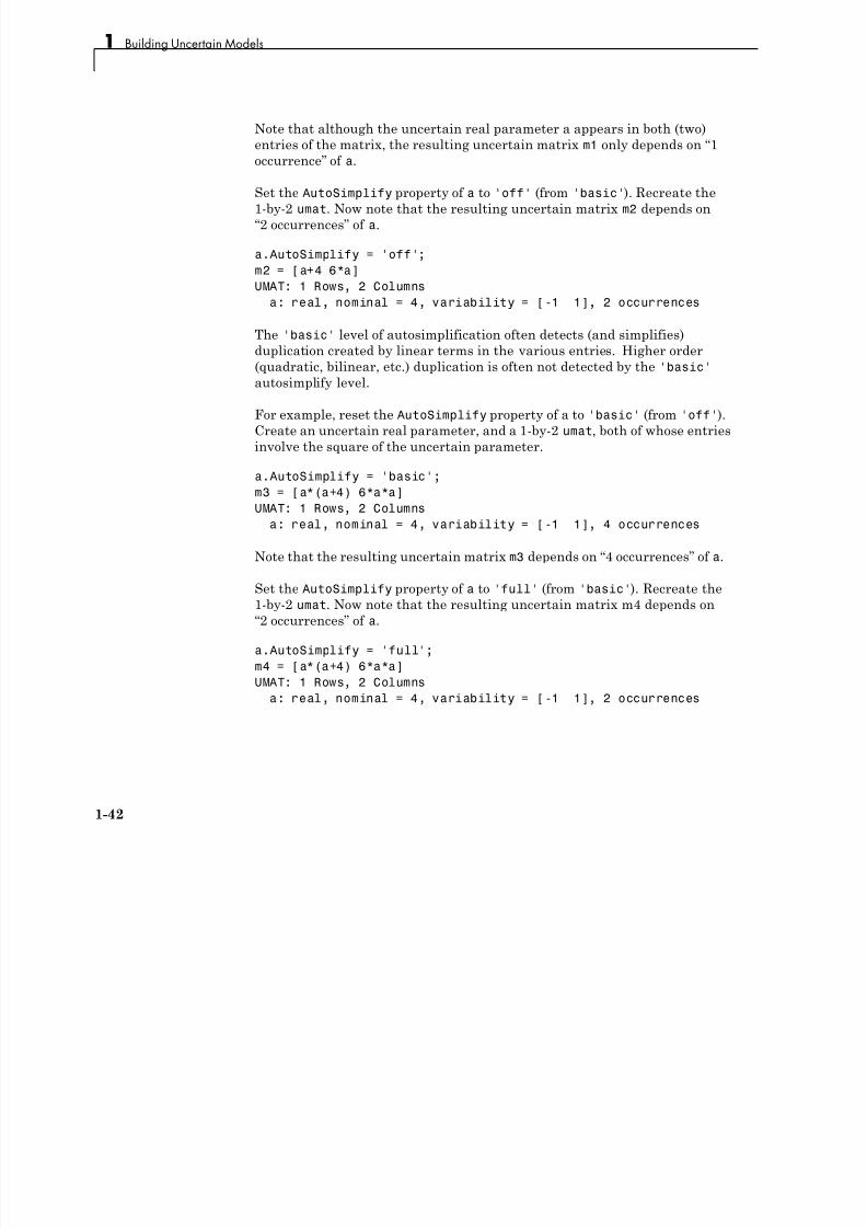
Note that although the uncertain real parameter a appears in both (two)
entries of the matrix, the resulting uncertain matrix m1 only depends on “1occurrence” of a.
Set the AutoSimplify property of a to 'off' (from 'basic'). Recreate the
1-by-2 umat. Now note that the resulting uncertain matrix m2 depends on
“2 occurrences” of a.
a.AutoSimplify = 'off';
m2 = [a+4 6*a]
UMAT: 1 Rows, 2 Columns
a: real, nominal = 4, variability = [-1 1], 2 occurrences
The 'basic' level of autosimplification often detects (and simplifies)
duplication created by linear terms in the various entries. Higher order
(quadratic, bilinear, etc.) duplication is often not detected by the 'basic'
autosimplify level.
For example, reset the AutoSimplify property of a to 'basic' (from 'off').
Create an uncertain real parameter, and a 1-by-2 umat, both of whose entries
involve the square of the uncertain parameter.
a.AutoSimplify = 'basic';
m3 = [a*(a+4) 6*a*a]
UMAT: 1 Rows, 2 Columns
a: real, nominal = 4, variability = [-1 1], 4 occurrences
Note that the resulting uncertain matrix m3 depends on “4 occurrences” of a.
Set the AutoSimplify property of a to 'full' (from 'basic'). Recreate the
1-by-2 umat. Now note that the resulting uncertain matrix m4 depends on
“2 occurrences” of a.
a.AutoSimplify = 'full';
m4 = [a*(a+4) 6*a*a]UMAT: 1 Rows, 2 Columns
a: real, nominal = 4, variability = [-1 1], 2 occurrences
1-42
Simplifying Representation of Uncertain Objects
7/30/2019 Robust Control Toolbox User's Guide
http://slidepdf.com/reader/full/robust-control-toolbox-users-guide 53/180
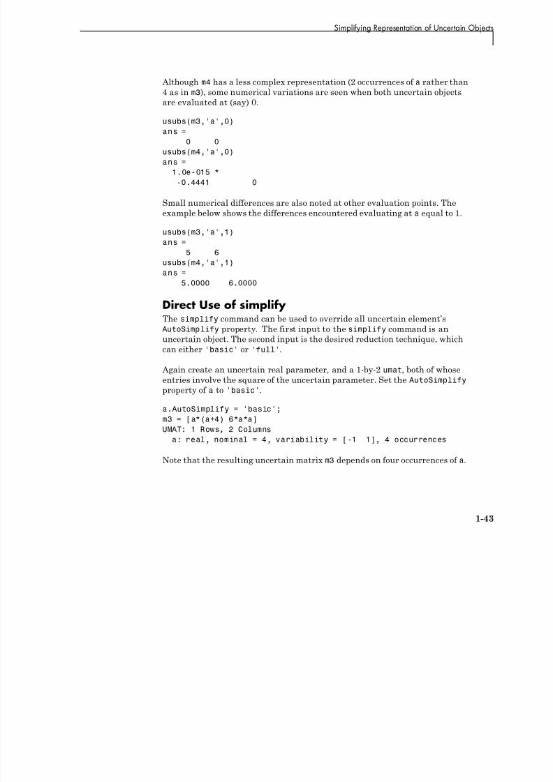
Although m4 has a less complex representation (2 occurrences of a rather than
4 as in m3), some numerical variations are seen when both uncertain objectsare evaluated at (say) 0.
usubs(m3,'a',0)
ans =
0 0
usubs(m4,'a',0)
ans =
1.0e-015 *
-0.4441 0
Small numerical differences are also noted at other evaluation points. The
example below shows the differences encountered evaluating at a equal to 1.
usubs(m3,'a',1)
ans =
5 6
usubs(m4,'a',1)ans =
5.0000 6.0000
Direct Use of simplify The simplify command can be used to override all uncertain element’s
AutoSimplify property. The first input to the simplify command is an
uncertain object. The second input is the desired reduction technique, whichcan either 'basic' or 'full'.
Again create an uncertain real parameter, and a 1-by-2 umat, both of whose
entries involve the square of the uncertain parameter. Set the AutoSimplify
property of a to 'basic'.
a.AutoSimplify = 'basic';
m3 = [a*(a+4) 6*a*a]
UMAT: 1 Rows, 2 Columnsa: real, nominal = 4, variability = [-1 1], 4 occurrences
Note that the resulting uncertain matrix m3 depends on four occurrences of a.
1-43
1 Building Uncertain Models

7/30/2019 Robust Control Toolbox User's Guide
http://slidepdf.com/reader/full/robust-control-toolbox-users-guide 54/180
The simplify command can be used to perform a 'full' reduction on the
resulting umat.
m4 = simplify(m3,'full')
UMAT: 1 Rows, 2 Columns
a: real, nominal = 4, variability = [-1 1], 2 occurrences
The resulting uncertain matrix m4 depends on only two occurrences of a after
the reduction.
1-44
Sampling Uncertain Objects
7/30/2019 Robust Control Toolbox User's Guide
http://slidepdf.com/reader/full/robust-control-toolbox-users-guide 55/180
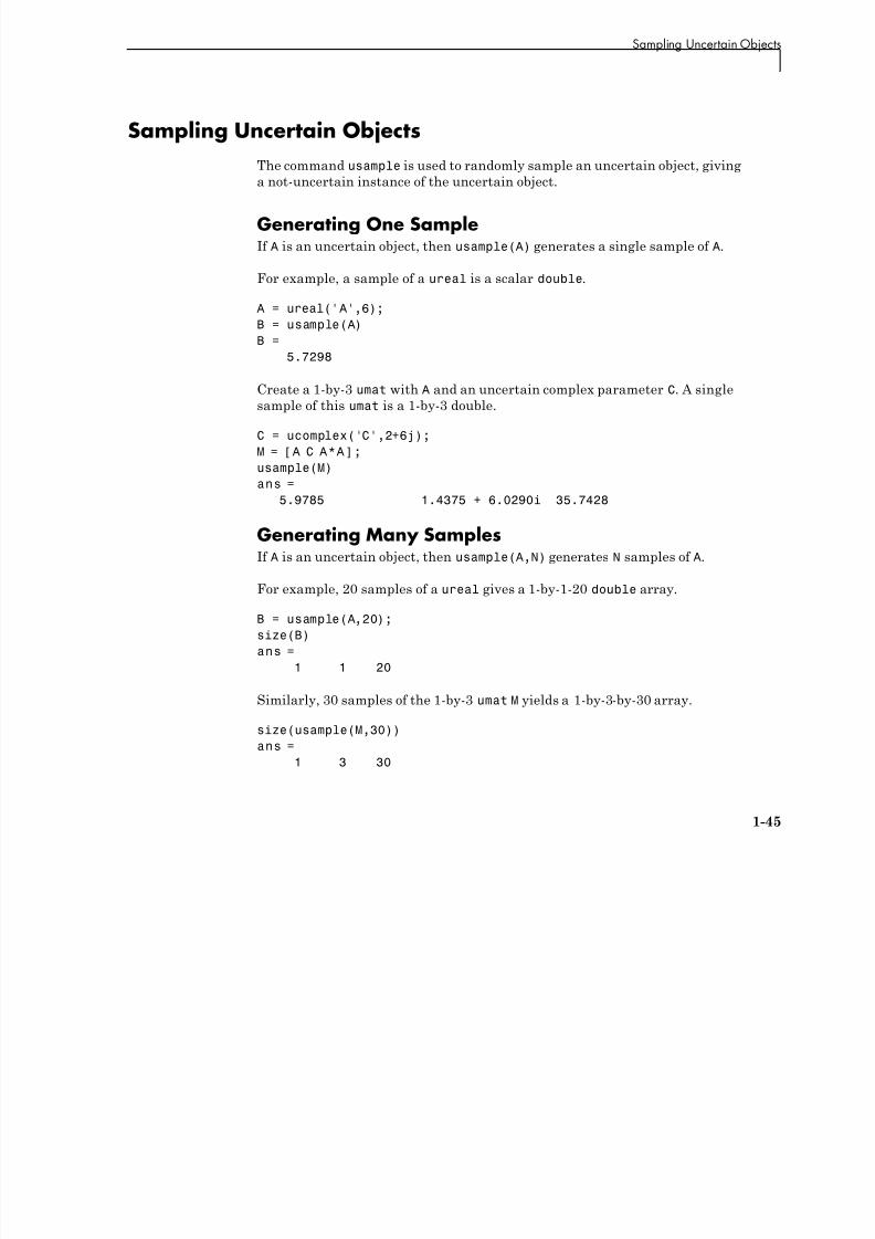
Sampling Uncertain Objects
The command usample is used to randomly sample an uncertain object, giving
a not-uncertain instance of the uncertain object.
Generating One SampleIf A is an uncertain object, then usample(A) generates a single sample of A.
For example, a sample of a ureal is a scalar double.
A = ureal('A',6);
B = usample(A)
B =
5.7298
Create a 1-by-3 umat with A and an uncertain complex parameter C. A single
sample of this umat is a 1-by-3 double.
C = ucomplex('C',2+6j);
M = [A C A*A];
usample(M)
ans =
5.9785 1.4375 + 6.0290i 35.7428
Generating Many SamplesIf A is an uncertain object, then usample(A,N) generates N samples of A.
For example, 20 samples of a ureal gives a 1-by-1-20 double array.
B = usample(A,20);
size(B)
ans =
1 1 20
Similarly, 30 samples of the 1-by-3 umat M yields a 1-by-3-by-30 array.
size(usample(M,30))
ans =
1 3 30
1-45
1 Building Uncertain Models

7/30/2019 Robust Control Toolbox User's Guide
http://slidepdf.com/reader/full/robust-control-toolbox-users-guide 56/180
See “Creating Arrays with usample” on page 1-57 for more information onsampling uncertain objects.
Sampling ultidyn AtomsWhen sampling a ultidyn atom (or an uncertain object that contains a
ultidyn atom in its Uncertainty gateway) the result is always a state-space
(ss) object. The property SampleStateDim of the ultidyn class determines
the state dimension of the samples.
Create a 1-by-1, gain bounded ultidyn object, with gain-bound 3. Verify that
the default state dimension for samples is 1.
del = ultidyn('del',[1 1],'Bound',3);
del.SampleStateDim
ans =
1
Sample the uncertain atom at 30 points. Verify that this creates a 30-by-1 ss
array of 1-input, 1-output, 1-state systems.
delS = usample(del,30);
size(delS)
30x1 array of state-space models
Each model has 1 output, 1 input, and 1 state.
Plot the Nyquist plot of these samples and add a disk of radius 3. Note that
the gain bound is satisfied and that the Nyquist plots are all circles, indicative
of 1st order systems.
nyquist(delS)
hold on;
theta = linspace(-pi,pi);
plot(del.Bound*exp(sqrt(-1)*theta),'r');hold off;
1-46
Sampling Uncertain Objects
7/30/2019 Robust Control Toolbox User's Guide
http://slidepdf.com/reader/full/robust-control-toolbox-users-guide 57/180
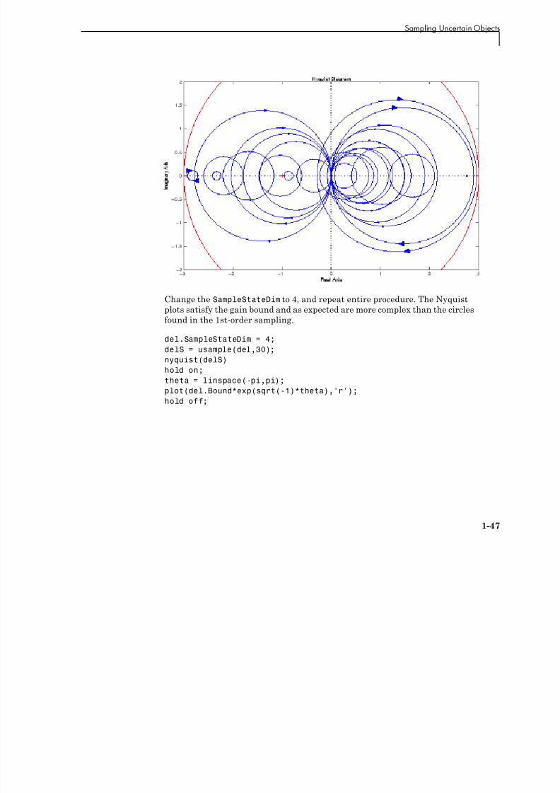
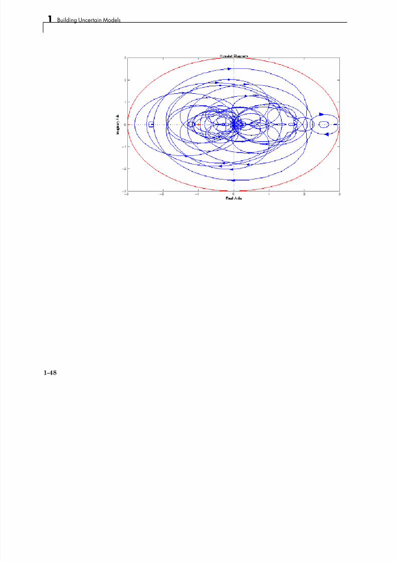
Change the SampleStateDim to 4, and repeat entire procedure. The Nyquist
plots satisfy the gain bound and as expected are more complex than the circles
found in the 1st-order sampling.
del.SampleStateDim = 4;
delS = usample(del,30);nyquist(delS)
hold on;
theta = linspace(-pi,pi);
plot(del.Bound*exp(sqrt(-1)*theta),'r');
hold off;
1-47
1 Building Uncertain Models
7/30/2019 Robust Control Toolbox User's Guide
http://slidepdf.com/reader/full/robust-control-toolbox-users-guide 58/180
1-48
Substitution by usubs
S b tit ti b b
7/30/2019 Robust Control Toolbox User's Guide
http://slidepdf.com/reader/full/robust-control-toolbox-users-guide 59/180
Substitution by usubs
If an uncertain object (umat, uss, ufrd) has many uncertain parameters, it
is often necessary to freeze some, but not all, of the uncertain parameters to
specific values. The usubs command accomplishes this, and also allows more
complicated substitutions for an atom.
usubs accepts a list of atom names, and respective values to substitute for
them. You can create three uncertain real parameters and use them to create
a 2-by-2 uncertain matrix A.
delta = ureal('delta',2);
eta = ureal('eta',6);
rho = ureal('rho',-1);
A = [3+delta+eta delta/eta;7+rho rho+delta*eta]
UMAT: 2 Rows, 2 Columns
delta: real, nominal = 2, variability = [-1 1], 2 occurrences
eta: real, nominal = 6, variability = [-1 1], 3 occurrences
rho: real, nominal = -1, variability = [-1 1], 1 occurrence
Use usubs to substitute the uncertain element named delta in A with the
value 2.3, leaving all other uncertain atoms intact. Note that the result, B, is
an uncertain matrix with dependence only on eta and rho.
B = usubs(A,'delta',2.3)
UMAT: 2 Rows, 2 Columns
eta: real, nominal = 6, variability = [-1 1], 3 occurrencesrho: real, nominal = -1, variability = [-1 1], 1 occurrence
To set multiple atoms, list individually, or in cells. The following are the same
B1 = usubs(A,'delta',2.3,'eta',A.Uncertainty.rho);
B2 = usubs(A,{'delta';'eta'},{2.3;A.Uncertainty.rho});
In each case, delta is replaced by 2.3, and eta is replaced by A.Uncertainty.rho.
If it makes sense, a single replacement value can be used to replace multiple
atoms. So
B3 = usubs(A,{'delta';'eta'},2.3);
1-49
1 Building Uncertain Models

7/30/2019 Robust Control Toolbox User's Guide
http://slidepdf.com/reader/full/robust-control-toolbox-users-guide 60/180
replaces both the atoms delta and eta with the real number 2.3. Anysuperfluous substitution requests are ignored. Hence
B4 = usubs(A,'fred',5);
is the same as A, and
B5 = usubs(A,{'delta';'eta'},2.3,{'fred' 'gamma'},0);
is the same as B3.
Specifying the Substitution with Structures An alternative syntax for usubs is to specify the substituted values in a
structure, whose fieldnames are the names of the atoms being substituted
with values.
Create a structure NV with 2 fields, delta and eta. Set the values of thesefields to be the desired substituted values. Then perform the substitution
with usubs.
NV.delta = 2.3;
NV.eta = A.Uncertainty.rho;
B6 = usubs(A,NV);
Here, B6 is the same as B1 and B2 above. Again, any superfluous fields areignored. Therefore, adding an additional field gamma to NV, and substituting
does not alter the result.
NV.gamma = 0;
B7 = usubs(A,NV);
Here, B7 is the same as B6.
The commands wcgain, robuststab and usample all return substitutable
values in this structure format. More discussion can be found in “Creating
Arrays with usubs” on page 1-58.
1-50
Substitution by usubs
Nominal and Random Values
7/30/2019 Robust Control Toolbox User's Guide
http://slidepdf.com/reader/full/robust-control-toolbox-users-guide 61/180
Nominal and Random Values
If the replacement value is the (partial and case-independent) string'Nominal', then the listed atom are replaced with their nominal values.
Therefore
B8 = usubs(A,fieldnames(A.Uncertainty),'nom')
B8 =
11.0000 0.3333
6.0000 11.0000
B9 = A.NominalValueB9 =
11.0000 0.3333
6.0000 11.0000
are the same. It is possible to only set some of the atoms to NominalValues,
and would be the typical use of usubs with the 'nominal' argument.
Within A, set eta to its nominal value, delta to a random value (within its
range) and rho to a specific value, say 6.5
B10 = usubs(A,'eta','nom','delta','rand','rho',6.5)
B10 =
10.5183 0.2531
13.5000 15.6100
Unfortunately, the 'nominal' and 'Random' specifiers may not be used in
the structure format. However, explicitly setting a field of the structure toan atom’s nominal value, and then following (or preceeding) the call to usubs
with a call to usample (to generate the random samples) is acceptable, and
achieves the same effect.
1-51
1 Building Uncertain Models
Array Management for Uncertain Objects
7/30/2019 Robust Control Toolbox User's Guide
http://slidepdf.com/reader/full/robust-control-toolbox-users-guide 62/180
Array Management for Uncertain Objects
All of the uncertain system classes (uss, ufrd) may be multidimensional
arrays. This is intended to provide the same functionality as the LTI-arrays
of the Control System Toolbox software. The command size returns a row
vector with the sizes of all dimensions.
The first two dimensions correspond to the outputs and inputs of the system.
Any dimensions beyond are referred to as the array dimensions. Hence, if szM
= size(M), then szM(3:end) are sizes of the array dimensions of M.
For these types of objects, it is clear that the first two dimensions (system
output and input) are interpreted differently from the 3rd, 4th, 5th and
higher dimensions (which often model parametrized variability in the system
input/output behavior).
umat objects are treated in the same manner. The first two dimensions are
the rows and columns of the uncertain matrix. Any dimensions beyond arethe array dimensions.
Referencing ArraysSuppose M is a umat, uss or ufrd, and that Yidx and Uidx are vectors of
integers. Then
M(Yidx,Uidx)
selects the outputs (rows) referred to by Yidx and the inputs (columns)
referred to by Uidx, preserving all of the array dimensions. For example, if
size(M) equals [ 4 5 3 6 7 ], then (for example) the size of M([4 2],[1 2
4]) is [ 2 3 3 6 7 ].
If size(M,1)==1 or size(M,2)==1, then single indexing on the inputs or
outputs (rows or columns) is allowed. If Sidx is a vector of integers, then
M(Sidx) selects the corresponding elements. All array dimensions arepreserved.
If there are K array dimensions, and idx1, idx2, ..., idxK are vectors
of integers, then
1-52
Array Management for Uncertain Objects
G = M(Yidx,Uidx,idx1,idx2,...,idxK)

7/30/2019 Robust Control Toolbox User's Guide
http://slidepdf.com/reader/full/robust-control-toolbox-users-guide 63/180
G M(Yidx,Uidx,idx1,idx2,...,idxK)
selects the outputs and inputs referred to by Yidx and Uidx, respectively,
and selects from each array dimension the “slices” referred to by the
idx1, idx2,..., idxK index vectors. Consequently, size(G,1) equals
length(Yidx), size(G,2) equals length(Uidx), size(G,3) equals
length(idx1), size(G,4) equals length(idx2), and size(G,K+2) equals
length(idxK).
If M has K array dimensions, and less than K index vectors are used in doing
the array referencing, then the MATLAB convention for single indexing
is followed. For instance, suppose size(M) equals [ 3 4 6 5 7 4 ]. The
expression
G = M([1 3],[1 4],[2 3 4],[5 3 1],[8 10 12 2 4 20 18])
is valid. The result has size(G) equals [ 2 2 3 3 7 ] . The last index vector[ 8 1 0 1 2 2 4 2 0 1 8 ] is used to reference into the 7-by-4 array, preserving
the order dictated by MATLAB single indexing (e.g., the 10th element of a7-by-4 array is the element in the (3,2) position in the array).
Note that if M has either one output (row) or one input (column), and M has
array dimensions, then it is not allowable to combine single indexing in the
output/input dimensions along with indexing in the array dimensions. This
will result in an ambiguity in how to interpret the second index vector in the
expression (i.e., “does it correspond to the input/output reference, or does it
correspond to the first array dimension?”).
Creating Arrays with stack and cat Functions An easy manner to create an array is with stack. Create a [4-by-1] umat
array by stacking four 1-by-3 umat objects with the stack command. The first
argument of stack specifies in which array dimension the stacking occurs. In
the example below, the stacking is done is the 1st array dimension, hence the
result is a 1-by-3-by-4-by-1 umat, referred to as a 4-by-1 umat array.
a = ureal('a',4);
b = ureal('b',2);
M = stack(1,[a b 1],[-a -b 4+a],[4 5 6],[a 0 0])
UMAT: 1 Rows, 3 Columns [array, 4 x 1]
1-53
1 Building Uncertain Models
a: real, nominal = 4, variability = [-1 1], 1 occurrence
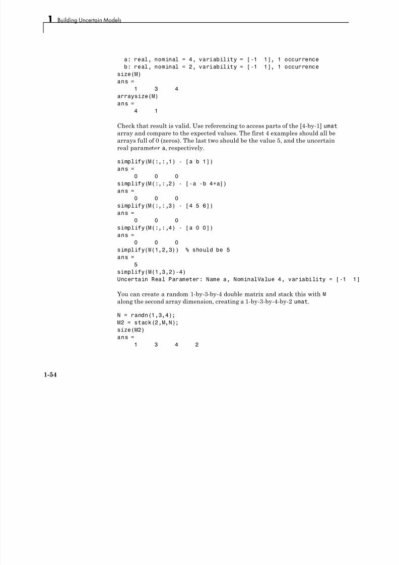
7/30/2019 Robust Control Toolbox User's Guide
http://slidepdf.com/reader/full/robust-control-toolbox-users-guide 64/180
, , y [ ],
b: real, nominal = 2, variability = [-1 1], 1 occurrencesize(M)
ans =
1 3 4
arraysize(M)
ans =
4 1
Check that result is valid. Use referencing to access parts of the [4-by-1] umat
array and compare to the expected values. The first 4 examples should all be
arrays full of 0 (zeros). The last two should be the value 5, and the uncertain
real parameter a, respectively.
simplify(M(:,:,1) - [a b 1])
ans =
0 0 0
simplify(M(:,:,2) - [-a -b 4+a])
ans =0 0 0
simplify(M(:,:,3) - [4 5 6])
ans =
0 0 0
simplify(M(:,:,4) - [a 0 0])
ans =
0 0 0
simplify(M(1,2,3)) % should be 5ans =
5
simplify(M(1,3,2)-4)
Uncertain Real Parameter: Name a, NominalValue 4, variability = [-1 1]
You can create a random 1-by-3-by-4 double matrix and stack this with M
along the second array dimension, creating a 1-by-3-by-4-by-2 umat.
N = randn(1,3,4);
M2 = stack(2,M,N);
size(M2)
ans =
1 3 4 2
1-54
Array Management for Uncertain Objects
arraysize(M2)

7/30/2019 Robust Control Toolbox User's Guide
http://slidepdf.com/reader/full/robust-control-toolbox-users-guide 65/180
ans =4 2
As expected, both M and N can be recovered from M2.
d1 = simplify(M2(:,:,:,1)-M);
d2 = simplify(M2(:,:,:,2)-N);
[max(abs(d1(:))) max(abs(d2(:)))]
ans =
0 0
It is also possible to stack M and N along the 1st array dimension, creating a
1-by-3-by-8-by-1 umat.
M3 = stack(1,M,N);
size(M3)
ans =
1 3 8arraysize(M3)
ans =
8 1
As expected, both M and N can be recovered from M3.
d3 = simplify(M3(:,:,1:4)-M);
d4 = simplify(M3(:,:,5:8)-N);[max(abs(d3(:))) max(abs(d4(:)))]
ans =
0 0
Creating Arrays by Assignment Arrays can be created by direct assignment. As with other MATLAB classes,
there is no need to preallocate the variable first. Simply assign elements – all
resizing is performed automatically.
For instance, an equivalent construction to
a = ureal('a',4);
b = ureal('b',2);
1-55
1 Building Uncertain Models
M = stack(1,[a b 1],[-a -b 4+a],[4 5 6],[a 0 0]);
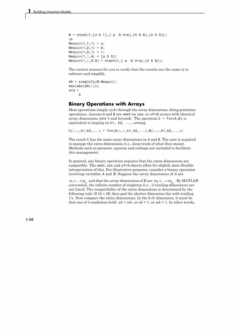
7/30/2019 Robust Control Toolbox User's Guide
http://slidepdf.com/reader/full/robust-control-toolbox-users-guide 66/180
isMequiv(1,1,1) = a;
Mequiv(1,2,1) = b;
Mequiv(1,3,1) = 1;
Mequiv(1,:,4) = [a 0 0];
Mequiv(1,:,2:3) = stack(1,[-a -b 4+a],[4 5 6]);
The easiest manner for you to verify that the results are the same is to
subtract and simplify,
d5 = simplify(M-Mequiv);
max(abs(d5(:)))
ans =
0
Binary Operations with Arrays
Most operations simply cycle through the array dimensions, doing pointwiseoperations. Assume A and B are umat (or uss, or ufrd) arrays with identical
array dimensions (slot 3 and beyond). The operation C = fcn(A,B) is
equivalent to looping on k1, k2, ..., setting
C(:,:,k1,k2,...) = fcn(A(:,:,k1,k2,...),B(:,:,k1,k2,...))
The result C has the same array dimensions as A and B. The user is required
to manage the extra dimensions (i.e., keep track of what they mean).
Methods such as permute, squeeze and reshape are included to facilitate
this management.
In general, any binary operation requires that the extra-dimensions are
compatible. The umat, uss and ufrd objects allow for slightly more flexible
interpretation of this. For illustrative purposes, consider a binary operation
involving variables A and B. Suppose the array dimensions of A are
n nl A1 × × and that the array dimensions of B are m ml B1 × × . By MATLABconvention, the infinite number of singleton (i.e., 1) trailing dimensions are
not listed. The compatibility of the extra dimensions is determined by the
following rule: If lA = lB, then pad the shorter dimension list with trailing
1’s. Now compare the extra dimensions: In the k-th dimension, it must be
that one of 3 conditions hold: nk = mk, or nk = 1, or mk = 1. In other words,
1-56
Array Management for Uncertain Objects
non-singleton dimensions must exactly match (so that the pointwise operation

7/30/2019 Robust Control Toolbox User's Guide
http://slidepdf.com/reader/full/robust-control-toolbox-users-guide 67/180
can be executed), and singleton dimensions match with anything, implicitlythrough a repmat.
Creating Arrays with usample An extremely common manner in which to generate an array is to sample (in
some of the uncertain elements) an uncertain object. Using the ureal objects
a and b from above, create a 2-by-3 umat.
M = [a b;b*b a/b;1-b 1+a*b]UMAT: 3 Rows, 2 Columns
a: real, nominal = 4, variability = [-1 1], 3 occurrences
b: real, nominal = 2, variability = [-1 1], 6 occurrences
size(M)
ans =
3 2
Sample (at 20 random points within its range) the uncertain real parameter bin the matrix M. This results in a 3-by-2-by-20 umat, with only one uncertain
element, a The uncertain element b of M has been “sampled out”, leaving
a new array dimension in its place.
[Ms,bvalues] = usample(M,'b',20);
Ms
UMAT: 3 Rows, 2 Columns [array, 20 x 1]
a: real, nominal = 4, variability = [-1 1], 2 occurrencessize(Ms)
ans =
3 2 20
Continue sampling (at 15 random points within its range) the uncertain real
parameter a in the matrix Ms. This results in a 3-by-2-by-20-by-15 double.
[Mss,avalues] = usample(Ms,'a',15);
size(Mss)ans =
3 2 20 15
class(Mss)
ans =
double
1-57
1 Building Uncertain Models
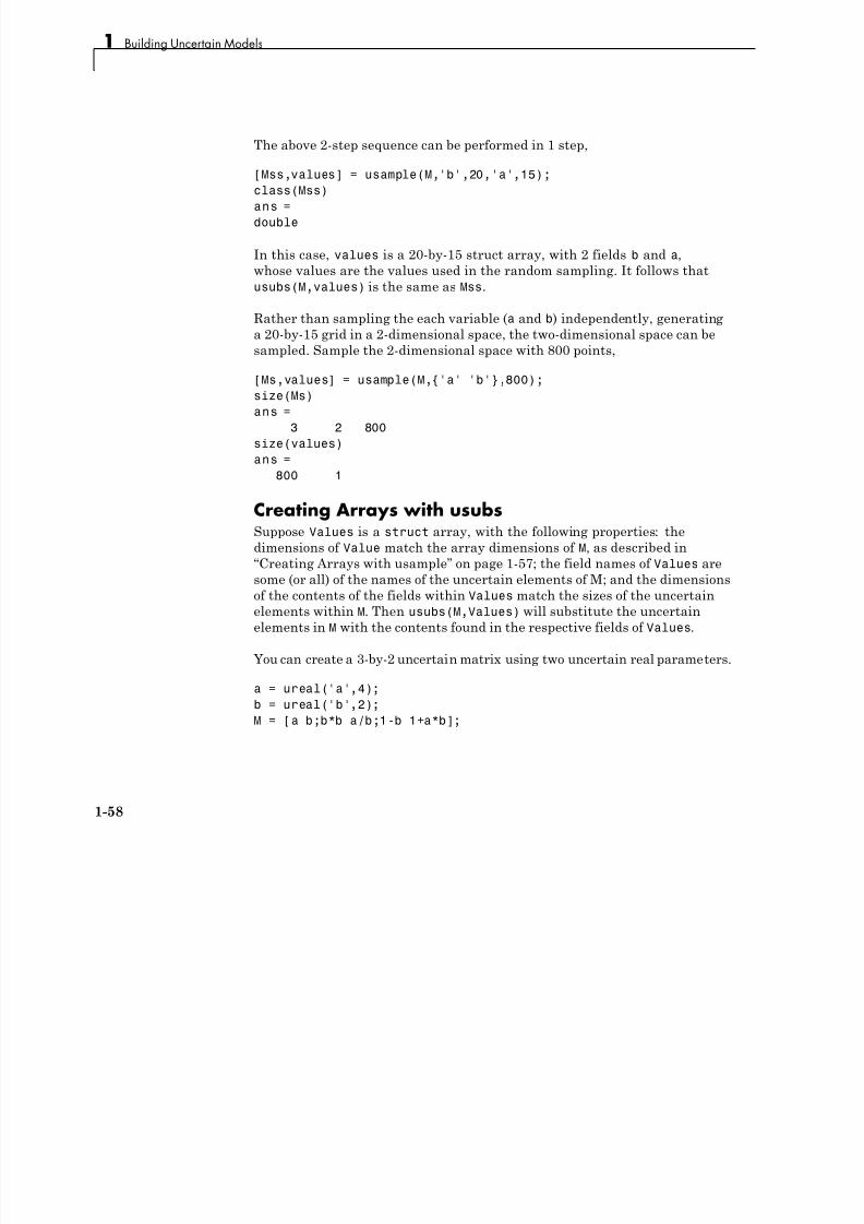
7/30/2019 Robust Control Toolbox User's Guide
http://slidepdf.com/reader/full/robust-control-toolbox-users-guide 68/180
The above 2-step sequence can be performed in 1 step,
[Mss,values] = usample(M,'b',20,'a',15);
class(Mss)
ans =
double
In this case, values is a 20-by-15 struct array, with 2 fields b and a,
whose values are the values used in the random sampling. It follows that
usubs(M,values) is the same as Mss.
Rather than sampling the each variable (a and b) independently, generating
a 20-by-15 grid in a 2-dimensional space, the two-dimensional space can be
sampled. Sample the 2-dimensional space with 800 points,
[Ms,values] = usample(M,{'a' 'b'},800);
size(Ms)
ans =3 2 800
size(values)
ans =
800 1
Creating Arrays with usubsSuppose Values is a struct array, with the following properties: the
dimensions of Value match the array dimensions of M, as described in
“Creating Arrays with usample” on page 1-57; the field names of Values are
some (or all) of the names of the uncertain elements of M; and the dimensions
of the contents of the fields within Values match the sizes of the uncertain
elements within M. Then usubs(M,Values) will substitute the uncertain
elements in M with the contents found in the respective fields of Values.
You can create a 3-by-2 uncertain matrix using two uncertain real parameters.
a = ureal('a',4);
b = ureal('b',2);
M = [a b;b*b a/b;1-b 1+a*b];
1-58
Array Management for Uncertain Objects
Create a 5-by-1 struct array with field name a. Make its values random
scalars Create a 1-by-4 struct array with field name b

7/30/2019 Robust Control Toolbox User's Guide
http://slidepdf.com/reader/full/robust-control-toolbox-users-guide 69/180
scalars. Create a 1-by-4 struct array with field name b.
Avalue = struct('a',num2cell(rand(5,1)));
Bvalue = struct('b',num2cell(rand(1,4)));
Substitute the uncertain real parameter a in M with the values in Avalue,
yielding ma. Similarly substitute the uncertain real parameter b in M with
the values in Avalue, yielding mb.
ma = usubs(M,Avalue)UMAT: 3 Rows, 2 Columns [array, 5 x 1]
b: real, nominal = 2, variability = [-1 1], 6 occurrences
mb = usubs(M,Bvalue)
UMAT: 3 Rows, 2 Columns [array, 1 x 4]
a: real, nominal = 4, variability = [-1 1], 2 occurrences
Continue, substituting the uncertain real parameter b in ma with the values
in Bvalue, yielding mab. Do the analogous operation for mb, yielding mba.Subtract, and note that the difference is 0, as expected.
mab = usubs(ma,Bvalue);
mba = usubs(mb,Avalue);
thediff = mab-mba;
max(abs(thediff(:)))
ans =
4.4409e-016
Creating Arrays with gridurealThe command gridureal enables uniform sampling of specified uncertain
real parameters within an uncertain object. It is a specialized case of usubs.
gridureal removes a specified uncertain real parameter and adds an array
dimension (to the end of the existing array dimensions). The new array
dimension represents the uniform samples of the uncertain object in thespecified uncertain real parameter range.
Create a 2-by-2 uncertain matrix with three uncertain real parameters.
a = ureal('a',3,'Range',[2.5 4]);
1-59
1 Building Uncertain Models
b = ureal('b',4,'Percentage',15);
c = ureal('c',-2,'Plusminus',[-1 .3]);
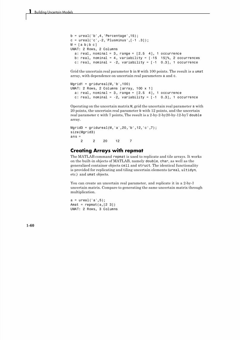
7/30/2019 Robust Control Toolbox User's Guide
http://slidepdf.com/reader/full/robust-control-toolbox-users-guide 70/180
c ureal( c , 2, Plusminus ,[ 1 .3]);
M = [ a b ; b c ]
UMAT: 2 Rows, 2 Columns
a: real, nominal = 3, range = [2.5 4], 1 occurrence
b: real, nominal = 4, variability = [-15 15]%, 2 occurrences
c: real, nominal = -2, variability = [-1 0.3], 1 occurrence
Grid the uncertain real parameter b in M with 100 points. The result is a umat
array, with dependence on uncertain real parameters a and c.
Mgrid1 = gridureal(M,'b',100)
UMAT: 2 Rows, 2 Columns [array, 100 x 1]
a: real, nominal = 3, range = [2.5 4], 1 occurrence
c: real, nominal = -2, variability = [-1 0.3], 1 occurrence
Operating on the uncertain matrix M, grid the uncertain real parameter a with
20 points, the uncertain real parameter b with 12 points, and the uncertain
real parameter c with 7 points, The result is a 2-by-2-by20-by-12-by7 doublearray.
Mgrid3 = gridureal(M,'a',20,'b',12,'c',7);
size(Mgrid3)
ans =
2 2 20 12 7
Creating Arrays with repmatThe MATLAB command repmat is used to replicate and tile arrays. It works
on the built-in objects of MATLAB, namely double, char, as well as the
generalized container objects cell and struct. The identical functionality
is provided for replicating and tiling uncertain elements (ureal, ultidyn,
etc.) and umat objects.
You can create an uncertain real parameter, and replicate it in a 2-by-3
uncertain matrix. Compare to generating the same uncertain matrix throughmultiplication.
a = ureal('a',5);
Amat = repmat(a,[2 3])
UMAT: 2 Rows, 3 Columns
1-60
Array Management for Uncertain Objects
a: real, nominal = 5, variability = [-1 1], 1 occurrence
Amat2 = a*ones(2,3);
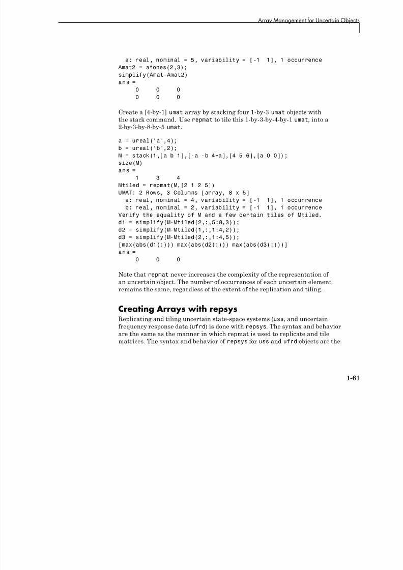
7/30/2019 Robust Control Toolbox User's Guide
http://slidepdf.com/reader/full/robust-control-toolbox-users-guide 71/180
( , );
simplify(Amat-Amat2)
ans =
0 0 0
0 0 0
Create a [4-by-1] umat array by stacking four 1-by-3 umat objects with
the stack command. Use repmat to tile this 1-by-3-by-4-by-1 umat, into a
2-by-3-by-8-by-5 umat.
a = ureal('a',4);
b = ureal('b',2);
M = stack(1,[a b 1],[-a -b 4+a],[4 5 6],[a 0 0]);
size(M)
ans =
1 3 4
Mtiled = repmat(M,[2 1 2 5])
UMAT: 2 Rows, 3 Columns [array, 8 x 5]a: real, nominal = 4, variability = [-1 1], 1 occurrence
b: real, nominal = 2, variability = [-1 1], 1 occurrence
Verify the equality of M and a few certain tiles of Mtiled.
d1 = simplify(M-Mtiled(2,:,5:8,3));
d2 = simplify(M-Mtiled(1,:,1:4,2));
d3 = simplify(M-Mtiled(2,:,1:4,5));
[max(abs(d1(:))) max(abs(d2(:))) max(abs(d3(:)))]
ans =0 0 0
Note that repmat never increases the complexity of the representation of
an uncertain object. The number of occurrences of each uncertain element
remains the same, regardless of the extent of the replication and tiling.
Creating Arrays with repsysReplicating and tiling uncertain state-space systems (uss, and uncertain
frequency response data (ufrd) is done with repsys. The syntax and behavior
are the same as the manner in which repmat is used to replicate and tile
matrices. The syntax and behavior of repsys for uss and ufrd objects are the
1-61
1 Building Uncertain Models
same as the traditional repsys which operates on ss and frd objects. Just as
in those cases, the uncertain version of repsys also allows for diagonal tiling.
7/30/2019 Robust Control Toolbox User's Guide
http://slidepdf.com/reader/full/robust-control-toolbox-users-guide 72/180
Using permute and ipermuteThe commands permute and ipermute are generalizations of transpose,
which exchanges the rows and columns of a two-dimensional matrix.
permute(A,ORDER) rearranges the dimensions of A so that they are in the
order specified by the vector ORDER. The array produced has the same values
of A but the order of the subscripts needed to access any particular elementare rearranged as specified by ORDER. The elements of ORDER must be a
rearrangement of the numbers from 1 to N.
All of the uncertain objects are essentially 2-dimensional (output and input)
operators with array dependence. This means that the first 2 dimensions are
treated differently from dimensions 3 and beyond. It is not permissible to
permute across these groups.
For uss and ufrd, the restriction is built into the syntax. The elements of the
ORDER vector only refer to array dimensions. Therefore, there is no possibility
of permute across these dimensions. In you need to permute the first two
dimensions, use the command transpose instead.
For umat, the restriction is enforced in the software. The elements of the
ORDER vector refer to all dimensions. However, the first two elements of ORDER
must be a rearrangement of the numbers 1 and 2. The remaining elements of ORDER must be a rearrangement of the numbers 3 through N. If either of those
conditions fail, an error is generated. Hence, for umat arrays, either permute
or transpose can be used to effect the transpose operation.
1-62
Decomposing Uncertain Objects (for Advanced Users)
Decomposing Uncertain Objects (for Advanced Users)

7/30/2019 Robust Control Toolbox User's Guide
http://slidepdf.com/reader/full/robust-control-toolbox-users-guide 73/180
Each uncertain object (umat, uss, ufrd) is a generalized feedback connection
(lft) of a not-uncertain object (e.g., double, ss, frd) with a diagonal
augmentation of uncertain atoms (ureal, ultidyn, ucomplex, ucomplexm,
udyn). In robust control jargon, if the uncertain elements are normalized, this
decomposition is often called “the M/D form.”
The purpose of the uncertain objects (ureal, ultidyn, umat, uss, etc.) is to
hide this underlying decomposition, and allow the user to focus on modeling
and analyzing uncertain systems, rather than the details of correctly
propagating the M/D representation in manipulations. Nevertheless,
advanced users may want access to the familiar M/D form. The command
lftdata accomplishes this decomposition.
Since ureal, ucomplex and ucomplexm do not have their NominalValue
necessarily at zero, and in the case of ureal objects, are not symmetric about
the NominalValue, some details are required in describing the decomposition.
Normalizing Functions for Uncertain Atoms Associated with each uncertain element is a normalizing function. The
normalizing function maps the uncertain element into a normalized uncertain
element.
If ρ is an uncertain real parameter, with range [L R] and nominal value N,
then the normalizing function F is
F A B
C D
( ) =
++
with the property that for all ρ satisfying L ≤ ρ ≤ R, it follows that –1 ≤ F ( ρ) ≤ 1,
moreover, F (L) = –1, F (N ) = 0, and F (R) = 1. If the nominal value is centered
in the range, then it is easy to conclude that
1-63
1 Building Uncertain Models
AR L
R L
=+

7/30/2019 Robust Control Toolbox User's Guide
http://slidepdf.com/reader/full/robust-control-toolbox-users-guide 74/180
R L B
R L
C
D
−=
−==
2
1
0.
It is left as an algebra exercise for the user to work out the various values for
A, B, C and D when the nominal value is not centered.
If E is an uncertain gain-bounded, linear, time-invariant dynamic uncertainty,
with gain-bound β, then the normalizing function F is
F E E( ) =1
.
If E is an uncertain positive-real, linear, time-invariant dynamic uncertainty,
with positivity bound β, then the normalizing function F is
F E I E I I E I ( ) = − −⎛ ⎝ ⎜
⎞ ⎠ ⎟
⎡
⎣⎢
⎤
⎦⎥ + −⎛
⎝ ⎜
⎞ ⎠ ⎟
⎡
⎣⎢
⎤
⎦⎥
−
2 2
1
where α = 2| β | + 1.
The normalizing function for an uncertain complex parameter ξ , with nominalvalue C and radius γ, is
F C
( ) = −( )1
.
The normalizing function for uncertain complex matrices H , with nominal
value N and weights W L and W R is
F H W H N W L R( ) = −( )− −1 1
1-64
Decomposing Uncertain Objects (for Advanced Users)
In each case, as the uncertain atom varies over its range, the absolute value
of the normalizing function (or norm, in the matrix case) varies from 0 and 1.
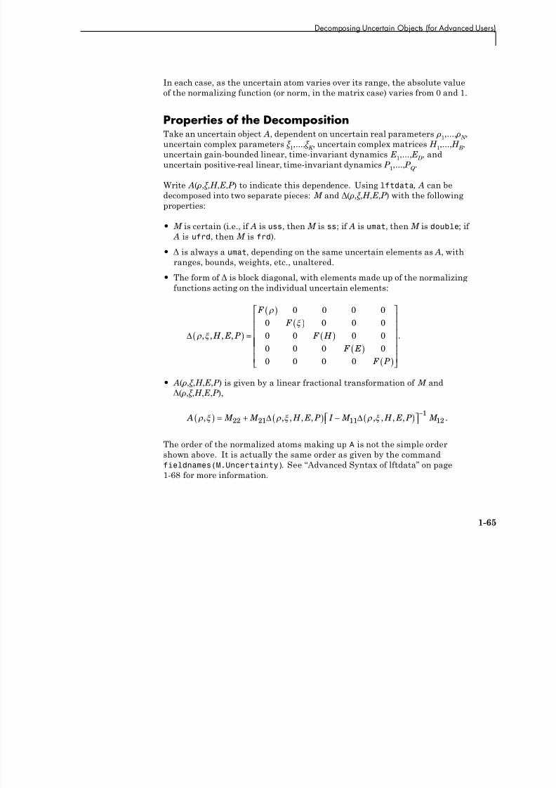
7/30/2019 Robust Control Toolbox User's Guide
http://slidepdf.com/reader/full/robust-control-toolbox-users-guide 75/180
Properties of the DecompositionTake an uncertain object A, dependent on uncertain real parameters ρ1,..., ρ
N ,
uncertain complex parameters ξ 1,...,ξ K
, uncertain complex matrices H 1,...,H B
,
uncertain gain-bounded linear, time-invariant dynamics E 1,...,E D
, and
uncertain positive-real linear, time-invariant dynamics P 1,..., P Q
.
Write A( ρ,ξ ,H ,E , P ) to indicate this dependence. Using lftdata, A can bedecomposed into two separate pieces: M and Δ( ρ,ξ ,H ,E , P ) with the following
properties:
• M is certain (i.e., if A is uss, then M is ss; if A is umat, then M is double; if A is ufrd, then M is frd).
• Δ is always a umat, depending on the same uncertain elements as A, with
ranges, bounds, weights, etc., unaltered.• The form of Δ is block diagonal, with elements made up of the normalizing
functions acting on the individual uncertain elements:
Δ
, , , , H E P
F
F
F H
F E F P
( ) =
( )
( )
( )
( )( )
⎡
⎣
⎢⎢⎢
0 0 0 0
0 0 0 0
0 0 0 0
0 0 0 00 0 0 0
⎢⎢⎢⎢
⎤
⎦
⎥⎥⎥⎥⎥⎥
.
• A( ρ,ξ ,H ,E , P ) is given by a linear fractional transformation of M and
Δ( ρ,ξ ,H ,E , P ),
A M M H E P I M H E P M , , , , , , , , , .( ) = + ( ) − ( )⎡⎣ ⎤⎦−
22 21 111
12Δ Δ
The order of the normalized atoms making up A is not the simple order
shown above. It is actually the same order as given by the command
fieldnames(M.Uncertainty). See “Advanced Syntax of lftdata” on page
1-68 for more information.
1-65
1 Building Uncertain Models
Syntax of lftdata
The decomposition is carried out by the command lftdata

7/30/2019 Robust Control Toolbox User's Guide
http://slidepdf.com/reader/full/robust-control-toolbox-users-guide 76/180
The decomposition is carried out by the command lftdata.
You can create a 2-by-2 umat named A using three uncertain real parameters.
delta = ureal('delta',2);
eta = ureal('eta',6);
rho = ureal('rho',-1);
A = [3+delta+eta delta/eta;7+rho rho+delta*eta]
UMAT: 2 Rows, 2 Columns
delta: real, nominal = 2, variability = [-1 1], 2 occurrences
eta: real, nominal = 6, variability = [-1 1], 3 occurrences
rho: real, nominal = -1, variability = [-1 1], 1 occurrence
Note that A depends on two occurrences of delta, three occurrences of eta
and one occurrence of rho.
Decompose A into M and Delta. Note that A is a double, and Delta has the
same uncertainty dependence as M.
[M,Delta] = lftdata(A);
class(M)
ans =
double
Delta
UMAT: 6 Rows, 6 Columns
delta: real, nominal = 2, variability = [-1 1], 2 occurrenceseta: real, nominal = 6, variability = [-1 1], 3 occurrences
rho: real, nominal = -1, variability = [-1 1], 1 occurrence
Sample Delta at 5 points. Things to note are:
• It is diagonal.
• The values range between -1 and 1.
• There are three independent values, and duplication of the entries is
consistent with the dependence of Delta and A on the three uncertain real
parameters.
usample(Delta,5)
1-66
Decomposing Uncertain Objects (for Advanced Users)
ans(:,:,1) =
-0.7106 0 0 0 0 0
0 -0.7106 0 0 0 0

7/30/2019 Robust Control Toolbox User's Guide
http://slidepdf.com/reader/full/robust-control-toolbox-users-guide 77/180
0 0.7106 0 0 0 0
0 0 0.6374 0 0 0
0 0 0 0.6374 0 0
0 0 0 0 0.6374 0
0 0 0 0 0 -0.1258
ans(:,:,2) =
-0.5850 0 0 0 0 0
0 -0.5850 0 0 0 0
0 0 -0.3021 0 0 00 0 0 -0.3021 0 0
0 0 0 0 -0.3021 0
0 0 0 0 0 0.0803
ans(:,:,3) =
0.7013 0 0 0 0 0
0 0.7013 0 0 0 0
0 0 -0.6749 0 0 0
0 0 0 -0.6749 0 00 0 0 0 -0.6749 0
0 0 0 0 0 0.3967
ans(:,:,4) =
0.4262 0 0 0 0 0
0 0.4262 0 0 0 0
0 0 0.0795 0 0 0
0 0 0 0.0795 0 0
0 0 0 0 0.0795 00 0 0 0 0 -0.9959
ans(:,:,5) =
-0.8392 0 0 0 0 0
0 -0.8392 0 0 0 0
0 0 0.8467 0 0 0
0 0 0 0.8467 0 0
0 0 0 0 0.8467 0
0 0 0 0 0 0.6732
In fact, verify that the maximum gain of Delta is indeed 1
maxnorm = wcnorm(Delta)
maxnorm =
1-67
1 Building Uncertain Models
LowerBound: 1.0000
UpperBound: 1.0004
7/30/2019 Robust Control Toolbox User's Guide
http://slidepdf.com/reader/full/robust-control-toolbox-users-guide 78/180
Finally, verify that lft(Delta,M) is the same as A Subtract (and use the
'full' option in simplify)
simplify(lft(Delta,M)-A,'full')
ans =
0 0
0 0
Advanced Syntax of lftdataEven for the advanced user, the variable Delta will actually not be that
useful, as it is still a complex object. On the other hand, its internal structure
is described completely using a 3rd (and 4th) output argument.
[M,Delta,BlkStruct,NormUnc] = lftdata(A);
The rows of BlkStruct correspond to the uncertain atoms named infieldnames(A.Uncertainty). Note that the range/bound information about
each uncertain atom is not included in BlkStruct.
The elements of BlkStruct describe the size, type and number-of-copies of
the uncertain atoms in A, and implicitly delineate the exact block-diagonal
structure of Delta. Note that the range/bound information about each
uncertain atom is not included in BlkStruct.
BlkStruct(1)
ans =
Name: 'delta'
Size: [1 1]
Type: 'ureal'
Occurrences: 2
BlkStruct(2)
ans =Name: 'eta'
Size: [1 1]
Type: 'ureal'
Occurrences: 3
BlkStruct(3)
1-68
Decomposing Uncertain Objects (for Advanced Users)
ans =
Name: 'rho'
Size: [1 1]

7/30/2019 Robust Control Toolbox User's Guide
http://slidepdf.com/reader/full/robust-control-toolbox-users-guide 79/180
Type: 'ureal'
Occurrences: 1
Together, these mean Delta is a block diagonal augmentation of the
normalized version of 3 uncertain atoms.
The first atom is named 'delta'. It is 1-by-1; it is of class ureal; and there
are 2 copies diagonally augmented.
The second atom is named 'eta'. It is 1-by-1; it is of class ureal; and there
are 3 copies diagonally augmented.
The third atom is named 'rho'. It is 1-by-1; it is of class ureal; and there
is 1 copy,
The 4th output argument contains a cell array of normalized uncertainelements. The cell array contains as many occurrences of each element as
there are occurrences in the original uncertain object A.
size(NormUnc)
ans =
6 1
NormUnc{1}
Uncertain Real Parameter: Name deltaNormalized, NominalValue 0,variability = [-1 1]
isequal(NormUnc{2},NormUnc{1})
ans =
1
NormUnc{3}
Uncertain Real Parameter: Name etaNormalized, NominalValue 0,
variability = [-1 1]
isequal(NormUnc{4},NormUnc{3})
ans =
1
isequal(NormUnc{5},NormUnc{3})
ans =
1
1-69
1 Building Uncertain Models
NormUnc{6}
Uncertain Real Parameter: Name rhoNormalized, NominalValue 0,
variability = [-1 1]

7/30/2019 Robust Control Toolbox User's Guide
http://slidepdf.com/reader/full/robust-control-toolbox-users-guide 80/180
Each normalized element has the string 'Normalized' appended to its
original name to avoid confusion. By normalized,
• ureal objects have nominal value of 0, and range from -1 to 1.
• ultidyn objects are norm bounded, with norm bound of 1.
• ucomplex objects have nominal value of 0, and radius 1.
• ucomplexm objects have nominal value of 0, and identity matrices for each
of the WL and WR weights.
The possible behaviors of Delta and blkdiag(NormUnc{:}) are the same.
Consequently, the possible behaviors of A and lft(blkdiag(NormUnc{:}),M)
are the same.
Hence, by manipulating M, BlkStruct and NormUnc, a power-user has direct
access to all of the linear fractional transformation details, and can easily
work at the level of the theorems and algorithms that underlie the methods.
1-70
2
Generalized Robustness
7/30/2019 Robust Control Toolbox User's Guide
http://slidepdf.com/reader/full/robust-control-toolbox-users-guide 81/180
Generalized Robustness Analysis
• “Introduction to Generalized Robustness Analysis” on page 2-2
• “Robust Stability Margin” on page 2-4
• “Robust Performance Margin” on page 2-5
• “Worst-Case Gain Measure” on page 2-6
2 Generalized Robustness Analysis
Introduction to Generalized Robustness Analysis
The performance of a nominally stable uncertain system model will generally
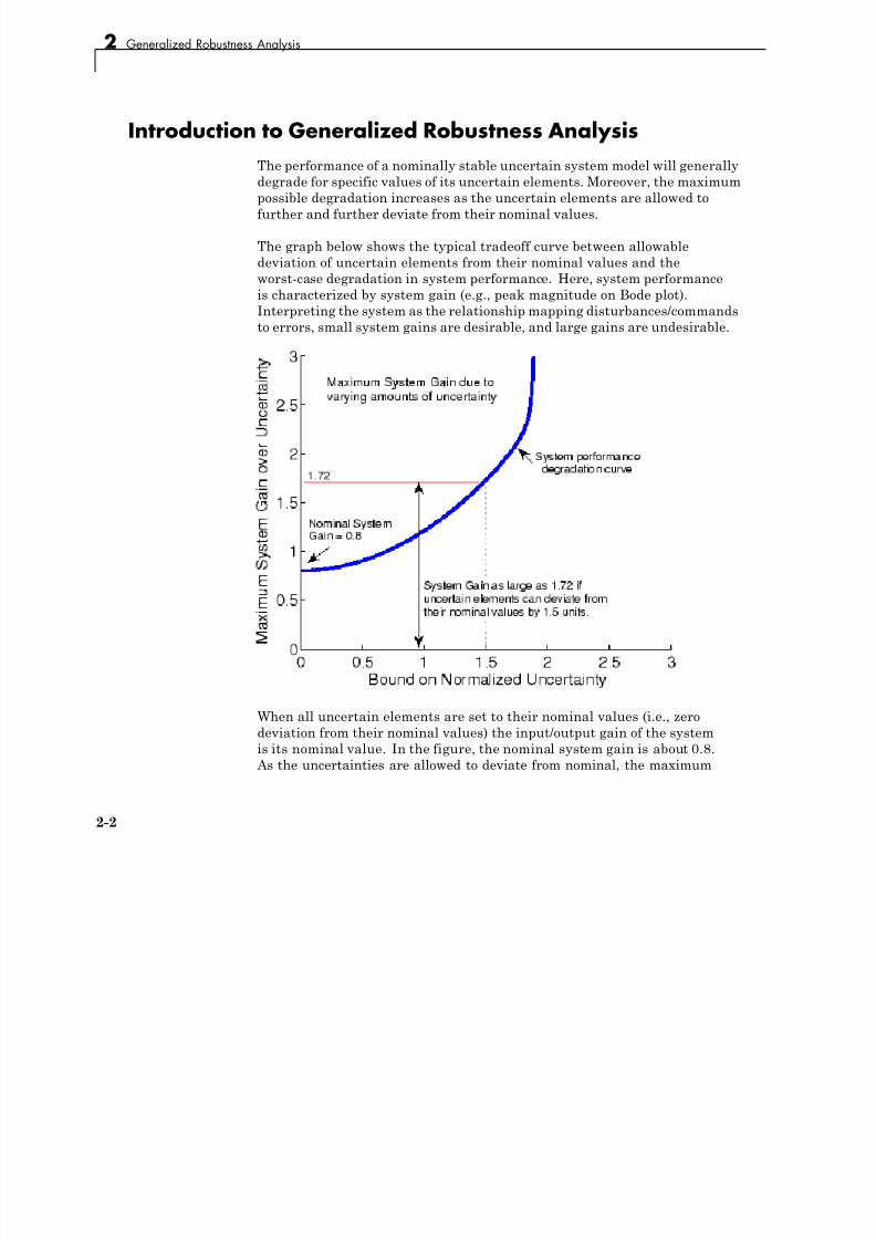
7/30/2019 Robust Control Toolbox User's Guide
http://slidepdf.com/reader/full/robust-control-toolbox-users-guide 82/180
degrade for specific values of its uncertain elements. Moreover, the maximum
possible degradation increases as the uncertain elements are allowed to
further and further deviate from their nominal values.
The graph below shows the typical tradeoff curve between allowable
deviation of uncertain elements from their nominal values and the
worst-case degradation in system performance. Here, system performance
is characterized by system gain (e.g., peak magnitude on Bode plot).Interpreting the system as the relationship mapping disturbances/commands
to errors, small system gains are desirable, and large gains are undesirable.
When all uncertain elements are set to their nominal values (i.e., zero
deviation from their nominal values) the input/output gain of the system
is its nominal value. In the figure, the nominal system gain is about 0.8.
As the uncertainties are allowed to deviate from nominal, the maximum
2-2
Introduction to Generalized Robustness Analysis
(over the uncertain elements) system gain increases. The heavy blue line
represents the maximum system gain due to uncertainty of various sizes (the
horizontal axis). and is called the system performance degradation curve. Itis monotonically increasing
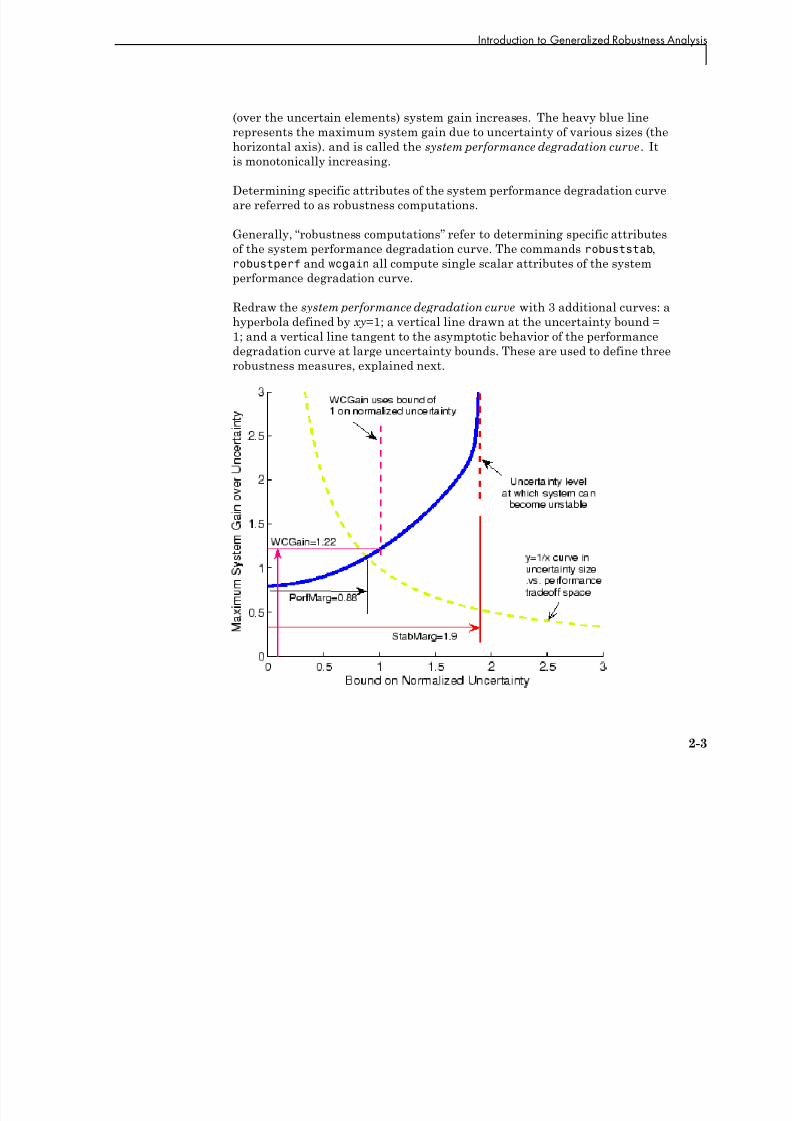
7/30/2019 Robust Control Toolbox User's Guide
http://slidepdf.com/reader/full/robust-control-toolbox-users-guide 83/180
is monotonically increasing.
Determining specific attributes of the system performance degradation curve
are referred to as robustness computations.
Generally, “robustness computations” refer to determining specific attributes
of the system performance degradation curve. The commands robuststab,
robustperf and wcgain all compute single scalar attributes of the systemperformance degradation curve.
Redraw the system performance degradation curve with 3 additional curves: a
hyperbola defined by xy=1; a vertical line drawn at the uncertainty bound =
1; and a vertical line tangent to the asymptotic behavior of the performance
degradation curve at large uncertainty bounds. These are used to define three
robustness measures, explained next.
2-3
2 Generalized Robustness Analysis
Robust Stability Margin
The robust stability margin, StabMarg, is the size of the smallest deviation
from nominal of the uncertain elements that leads to system instability

7/30/2019 Robust Control Toolbox User's Guide
http://slidepdf.com/reader/full/robust-control-toolbox-users-guide 84/180
from nominal of the uncertain elements that leads to system instability.
System instability is equivalent to the system gain becoming arbitrarily
large, and hence characterized by the vertical line tangent to the asymptotic
behavior of the performance degradation curve.
2-4
Robust Performance Margin
Robust Performance Margin
The hyperbola is used to define the performance margin. Systems whose
performance degradation curve intersects high on the hyperbola curve

7/30/2019 Robust Control Toolbox User's Guide
http://slidepdf.com/reader/full/robust-control-toolbox-users-guide 85/180
performance degradation curve intersects high on the hyperbola curve
represent “non-robustly performing systems” in that very small deviations
of the uncertain elements from their nominal values can result in very large
system gains. Conversely, an intersection low on the hyperbola represent
“robustly performing systems.”
The point where the system performance degradation curve crosses the green
line is used as a scalar measure of the robustness of a system to uncertainty.
The horizontal coordinate of the crossing point is the robust performance
margin, PerfMarg.
2-5
2 Generalized Robustness Analysis
Worst-Case Gain Measure
The worst-case gain measure is the maximum achievable system gain over all
uncertain elements whose normalized size is bounded by 1.

7/30/2019 Robust Control Toolbox User's Guide
http://slidepdf.com/reader/full/robust-control-toolbox-users-guide 86/180
uncertain elements whose normalized size is bounded by 1.
On the graph, this is the vertical coordinate of the performance degradation
curve as it crosses the vertical line drawn at the uncertainty bound = 1.
Each measure captures a single scalar attribute of the system performance
degradation curve. Mathematically, they are independent quantities,
answering subtlely different questions. Consequently, for two uncertain
systems, sysA and sysB, it is possible that the StabMarg of sysA is larger
than the StabMarg of sysB, though the PerfMarg of sysA is smaller than the
PerfMarg of sysB. Nevertheless, they are useful metrics for concise description
of the robustness of a system (uss or ufrd) due to various uncertain elements.
2-6
3
Introduction to Linear

7/30/2019 Robust Control Toolbox User's Guide
http://slidepdf.com/reader/full/robust-control-toolbox-users-guide 87/180
Introduction to LinearMatrix Inequalities
• “Linear Matrix Inequalities” on page 3-2
• “LMIs and LMI Problems” on page 3-4
• “Further Mathematical Background” on page 3-10
• “Bibliography” on page 3-11
3 Introduction to Linear Matrix Inequalities
Linear Matrix Inequalities
Linear Matrix Inequalities (LMIs) and LMI techniques have emerged aspowerful design tools in areas ranging from control engineering to system

7/30/2019 Robust Control Toolbox User's Guide
http://slidepdf.com/reader/full/robust-control-toolbox-users-guide 88/180
identification and structural design. Three factors make LMI techniques
appealing:
• A variety of design specifications and constraints can be expressed as LMIs.
• Once formulated in terms of LMIs, a problem can be solved exactly by
efficient convex optimization algorithms (see “LMI Solvers” on page 4-22).• While most problems with multiple constraints or objectives lack analytical
solutions in terms of matrix equations, they often remain tractable in the
LMI framework. This makes LMI-based design a valuable alternative to
classical “analytical” methods.
See [9] for a good introduction to LMI concepts. Robust Control Toolbox™
software is designed as an easy and progressive gateway to the new and
fast-growing field of LMIs:
• For users who occasionally need to solve LMI problems, the LMI Editor
and the tutorial introduction to LMI concepts and LMI solvers provide
for quick and easy problem solving.
• For more experienced LMI users, Chapter 4, “LMI Lab”, offers a rich,
flexible, and fully programmable environment to develop customized
LMI-based tools.
LMI FeaturesRobust Control Toolbox LMI functionality serves two purposes:
• Provide state-of-the-art tools for the LMI-based analysis and design of
robust control systems
• Offer a flexible and user-friendly environment to specify and solve general
LMI problems (the LMI Lab)
Examples of LMI-based analysis and design tools include
3-2
Linear Matrix Inequalities
• Functions to analyze the robust stability and performance of uncertain
systems with varying parameters (popov, quadstab, quadperf ...)
• Functions to design robust control with a mix of H2, H∞
, and pole placement
objectives (h2hinfsyn)

7/30/2019 Robust Control Toolbox User's Guide
http://slidepdf.com/reader/full/robust-control-toolbox-users-guide 89/180
j ( y )
• Functions for synthesizing robust gain-scheduled H∞
controllers (hinfgs)
For users interested in developing their own applications, the LMI Lab
provides a general-purpose and fully programmable environment to specify
and solve virtually any LMI problem. Note that the scope of this facility is by
no means restricted to control-oriented applications.
Note Robust Control Toolbox software implements state-of-the-art
interior-point LMI solvers. While these solvers are significantly faster than
classical convex optimization algorithms, you should keep in mind that the
complexity of LMI computations can grow quickly with the problem order
(number of states). For example, the number of operations required to solve
a Riccati equation is o(n3
) where n is the state dimension, while the cost of solving an equivalent “Riccati inequality” LMI is o(n6).
3-3
3 Introduction to Linear Matrix Inequalities
LMIs and LMI Problems
A linear matrix inequality (LMI) is any constraint of the form
A( ) A A A 0 (3-1)

7/30/2019 Robust Control Toolbox User's Guide
http://slidepdf.com/reader/full/robust-control-toolbox-users-guide 90/180
A(x ) := A0 + x 1 A1 + ... + x N A
N < 0 (3-1)
where
• x = (x 1, . . . , x N
) is a vector of unknown scalars (the decision or optimization
variables)
• A0, . . . , AN are given symmetric matrices
• < 0 stands for “negative definite,” i.e., the largest eigenvalue of A(x ) is
negative
Note that the constraints A(x ) > 0 and A(x ) < B(x ) are special cases of Equation
3-1 since they can be rewritten as – A(x ) < 0 and A(x ) – B(x ) < 0, respectively.
The LMI of Equation 3-1 is a convex constraint on x since A( y) < 0 and A(z) < 0
imply that
Ay z+⎛
⎝ ⎜
⎞ ⎠ ⎟ <
20
. As a result,
• Its solution set, called the feasible set, is a convex subset of RN
• Finding a solution x to Equation 3-1, if any, is a convex optimization
problem.
Convexity has an important consequence: even though Equation 3-1 has no
analytical solution in general, it can be solved numerically with guarantees
of finding a solution when one exists. Note that a system of LMI constraints
can be regarded as a single LMI since
A x
A x K
1 0
0
( ) <
( ) <
⎧
⎨⎪
⎩⎪
is equivalent to
3-4
LMIs and LMI Problems
A x x x( ) = ( ) ( )( ) <: , ,diag A A 1 K 0
where diag ( A1(x ), . . . , AK (x )) denotes the block-diagonal matrix with A1(x ), . . . , AK(x ) on its diagonal. Hence multiple LMI constraints can be

7/30/2019 Robust Control Toolbox User's Guide
http://slidepdf.com/reader/full/robust-control-toolbox-users-guide 91/180
1( ), , K ( ) g p
imposed on the vector of decision variables x without destroying convexity.
In most control applications, LMIs do not naturally arise in the canonical
form of Equation 3-1 , but rather in the form
L( X 1, . . . , X n) < R( X 1, . . . , X n)
where L(.) and R(.) are affine functions of some structured matrix variables X 1, . . . , X n. A simple example is the Lyapunov inequality
AT X + XA < 0 (3-2)
where the unknown X is a symmetric matrix. Defining x 1, . . . , x N as the
independent scalar entries of X , this LMI could be rewritten in the form of
Equation 3-1. Yet it is more convenient and efficient to describe it in itsnatural form Equation 3-2, which is the approach taken in the LMI Lab.
Three Generic LMI ProblemsFinding a solution x to the LMI system
A(x ) < 0 (3-3)
is called the feasibility problem. Minimizing a convex objective under LMI
constraints is also a convex problem. In particular, the linear objective
minimization problem:
Minimize cT x subject to
A(x ) < 0 (3-4)
plays an important role in LMI-based design. Finally, the generalizedeigenvalue minimization problem
Minimize λ subject to
3-5
3 Introduction to Linear Matrix Inequalities
A x B x
B x
C x
( ) < ( )
( ) >
( ) >
0
0 (3-5)
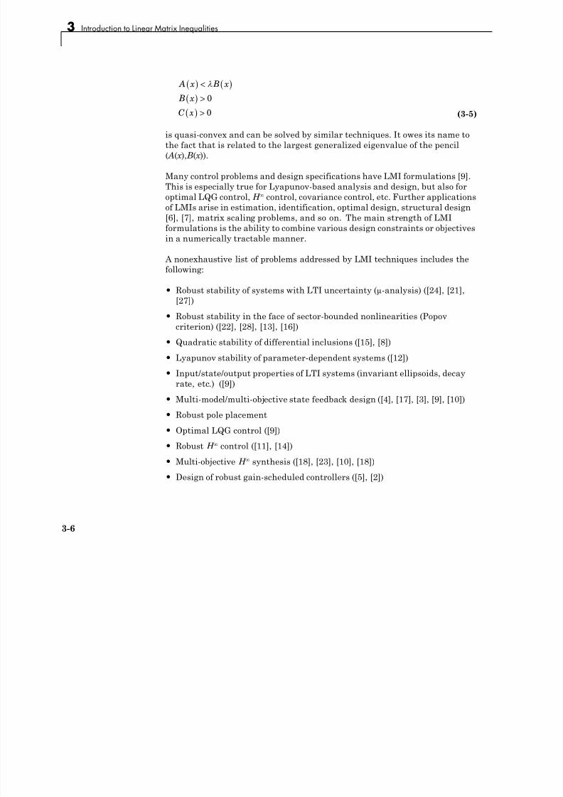
7/30/2019 Robust Control Toolbox User's Guide
http://slidepdf.com/reader/full/robust-control-toolbox-users-guide 92/180
is quasi-convex and can be solved by similar techniques. It owes its name to
the fact that is related to the largest generalized eigenvalue of the pencil
( A(x ), B(x )).
Many control problems and design specifications have LMI formulations [9].
This is especially true for Lyapunov-based analysis and design, but also foroptimal LQG control, H ∞ control, covariance control, etc. Further applications
of LMIs arise in estimation, identification, optimal design, structural design
[6], [7], matrix scaling problems, and so on. The main strength of LMI
formulations is the ability to combine various design constraints or objectives
in a numerically tractable manner.
A nonexhaustive list of problems addressed by LMI techniques includes the
following:
• Robust stability of systems with LTI uncertainty (µ-analysis) ([24], [21],
[27])
• Robust stability in the face of sector-bounded nonlinearities (Popov
criterion) ([22], [28], [13], [16])
• Quadratic stability of differential inclusions ([15], [8])
• Lyapunov stability of parameter-dependent systems ([12])
• Input/state/output properties of LTI systems (invariant ellipsoids, decay
rate, etc.) ([9])
• Multi-model/multi-objective state feedback design ([4], [17], [3], [9], [10])
• Robust pole placement
• Optimal LQG control ([9])
• Robust H ∞ control ([11], [14])
• Multi-objective H ∞ synthesis ([18], [23], [10], [18])
• Design of robust gain-scheduled controllers ([5], [2])
3-6
LMIs and LMI Problems
• Control of stochastic systems ([9])
•Weighted interpolation problems ([9])
To hint at the principles underlying LMI design, let’s review the LMI
f l ti f f t i l d i bj ti

7/30/2019 Robust Control Toolbox User's Guide
http://slidepdf.com/reader/full/robust-control-toolbox-users-guide 93/180
formulations of a few typical design objectives.
Stability The stability of the dynamic system
x Ax=
is equivalent to the feasibility of the following problem:
Find P = P T such that AT P + P A < 0, P > I.
This can be generalized to linear differential inclusions (LDI)
x A t x= ( )
where A(t) varies in the convex envelope of a set of LTI models:
A t C A A a A a an i i i ii
N
i
n
( ) ∈ { } = ≥ =⎧⎨⎪
⎩⎪
⎫⎬⎪
⎭⎪==∑∑o 1, , : , . 0 1
11
A sufficient condition for the asymptotic stability of this LDI is the feasibility
of
Find P = P T such that A P PA P I iT
i+ < >0, .
RMS Gain
The random-mean-squares (RMS) gain of a stable LTI system
x Ax Bu
y Cx Du
= += +
⎧⎨⎩
3-7
3 Introduction to Linear Matrix Inequalities
is the largest input/output gain over all bounded inputs u(t). This gain is
the global minimum of the following linear objective minimization problem
[1], [25], [26].
Minimize γ over X = X T and γ such that
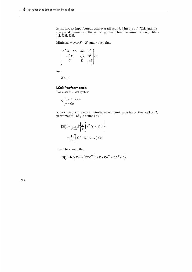
7/30/2019 Robust Control Toolbox User's Guide
http://slidepdf.com/reader/full/robust-control-toolbox-users-guide 94/180
A X XA XB C
B X I D
C D I
T T
T T
+
−−
⎛
⎝
⎜⎜⎜⎜
⎞
⎠
⎟ ⎟ ⎟ ⎟
<
0
and
X > 0.
LQG Performance
For a stable LTI system
G x Ax Bw
y Cx
= +=
⎧⎨⎩
where w is a white noise disturbance with unit covariance, the LQG or H 2performance G 2 is defined by
G ET
y t y t dt
G j G j d
T
T T
H
22
0
1
1
2
: lim
.
= ( ) ( )⎧⎨⎪
⎩⎪
⎫⎬⎪
⎭⎪
= ( ) ( )
→∞
−∞
∫
∞∞
∫
It can be shown that
G AP PA BBT T T 2
20= ( ) + + <{ }inf : .Trace CPC
3-8
LMIs and LMI Problems
Hence G22
is the global minimum of the LMI problem. Minimize Trace (Q )
over the symmetric matrices P ,Q such that
AP PA BBT T + + < 0

7/30/2019 Robust Control Toolbox User's Guide
http://slidepdf.com/reader/full/robust-control-toolbox-users-guide 95/180
and
Q CP
PC P
T
⎛
⎝
⎜⎜⎞
⎠
⎟ ⎟ > 0.
Again this is a linear objective minimization problem since the objective Trace
(Q ) is linear in the decision variables (free entries of P ,Q ).
3-9
3 Introduction to Linear Matrix Inequalities
Further Mathematical Background
Efficient interior-point algorithms are now available to solve the three genericLMI problems Equation 3-2 – Equation 3-4 defined in “Three Generic LMI
Problems” on page 3-5. These algorithms have a polynomial-time complexity.

7/30/2019 Robust Control Toolbox User's Guide
http://slidepdf.com/reader/full/robust-control-toolbox-users-guide 96/180
That is, the number N (ε) of flops needed to compute an ε-accurate solution is
bounded by
M N 3 log(V /ε)
where M is the total row size of the LMI system, N is the total number of scalar decision variables, and V is a data-dependent scaling factor. Robust
Control Toolbox software implements the Projective Algorithm of Nesterov
and Nemirovski [20], [19]. In addition to its polynomial-time complexity,
this algorithm does not require an initial feasible point for the linear
objective minimization problem Equation 3-3or the generalized eigenvalue
minimization problem Equation 3-4.
Some LMI problems are formulated in terms of inequalities rather than strictinequalities. For instance, a variant of Equation 3-3 is
Minimize cT x subject to A(x ) < 0.
While this distinction is immaterial in general, it matters when A(x ) can be
made negative semi-definite but not negative definite. A simple example is:
Minimize cT
x subject to
x x
x x
⎛
⎝ ⎜
⎞
⎠ ⎟ ≥ 0.
(3-6)
Such problems cannot be handled directly by interior-point methods which
require strict feasibility of the LMI constraints. A well-posed reformulation of
Equation 3-5 would be
Minimize cT x subject to x ≥ 0.
Keeping this subtlety in mind, we always use strict inequalities in this
manual.
3-10
Bibliography
Bibliography
[1] Anderson, B.D.O., and S. Vongpanitlerd, Network Analysis, Prentice-Hall,Englewood Cliffs, 1973.
[2] A k i P P G hi d G B k “S lf S h d l d H C l f

7/30/2019 Robust Control Toolbox User's Guide
http://slidepdf.com/reader/full/robust-control-toolbox-users-guide 97/180
[2] Apkarian, P., P. Gahinet, and G. Becker, “Self-Scheduled H ∞ Control of
Linear Parameter-Varying Systems,” Proc. Amer. Contr. Conf ., 1994, pp.
856-860.
[3] Bambang, R., E. Shimemura, and K. Uchida, “Mixed H 2 /H ∞ Control with
Pole Placement,” State-Feedback Case, Proc. Amer. Contr. Conf ., 1993, pp.2777-2779.
[4] Barmish, B.R., “Stabilization of Uncertain Systems via Linear Control,”IEEE Trans. Aut. Contr., AC–28 (1983), pp. 848-850.
[5] Becker, G., and Packard, P., “Robust Performance of Linear-Parametrically
Varying Systems Using Parametrically-Dependent Linear Feedback,” Systems
and Control Letters, 23 (1994), pp. 205-215.
[6] Bendsoe, M.P., A. Ben-Tal, and J. Zowe, “Optimization Methods for Truss
Geometry and Topology Design,” to appear in Structural Optimization.
[7] Ben-Tal, A., and A. Nemirovski, “Potential Reduction Polynomial-Time
Method for Truss Topology Design,” to appear in SIAM J. Contr. Opt.
[8] Boyd, S., and Q. Yang, “Structured and Simultaneous Lyapunov Functionsfor System Stability Problems,” Int. J. Contr., 49 (1989), pp. 2215-2240.
[9] Boyd, S., L. El Ghaoui, E. Feron, and V. Balakrishnan, Linear Matrix
Inequalities in Systems and Control Theory, SIAM books, Philadelphia, 1994.
[10] Chilali, M., and P. Gahinet, “H ∞ Design with Pole Placement Constraints:
an LMI Approach,” to appear in IEEE Trans. Aut. Contr. Also in Proc. Conf.
Dec. Contr., 1994, pp. 553-558.
[11] Gahinet, P., and P. Apkarian, “A Linear Matrix Inequality Approach toH ∞ Control,” Int. J. Robust and Nonlinear Contr., 4 (1994), pp. 421-448.
3-11
3 Introduction to Linear Matrix Inequalities
[12] Gahinet, P., P. Apkarian, and M. Chilali, “Affine Parameter-Dependent
Lyapunov Functions for Real Parametric Uncertainty,“ Proc. Conf. Dec.
Contr., 1994, pp. 2026-2031.
[13] Haddad, W.M., and D.S. Berstein, “Parameter-Dependent Lyapunov
Functions Constant Real Parameter Uncertainty and the Popov Criterion
7/30/2019 Robust Control Toolbox User's Guide
http://slidepdf.com/reader/full/robust-control-toolbox-users-guide 98/180
Functions, Constant Real Parameter Uncertainty, and the Popov Criterion
in Robust Analysis and Synthesis: Part 1 and 2,” Proc. Conf. Dec. Contr.,
1991, pp. 2274-2279 and 2632-2633.
[14] Iwasaki, T., and R.E. Skelton, “All Controllers for the General H ∞ Control
Problem: LMI Existence Conditions and State-Space Formulas,” Automatica,30 (1994), pp. 1307-1317.
[15] Horisberger, H.P., and P.R. Belanger, “Regulators for Linear
Time-Varying Plants with Uncertain Parameters,” IEEE Trans. Aut. Contr.,
AC–21 (1976), pp. 705-708.
[16] How, J.P., and S.R. Hall, “Connection between the Popov Stability
Criterion and Bounds for Real Parameter Uncertainty,” Proc. Amer. Contr.Conf ., 1993, pp. 1084-1089.
[17] Khargonekar, P.P., and M.A. Rotea, “Mixed H 2 /H ∞ Control: a Convex
Optimization Approach,” IEEE Trans. Aut. Contr., 39 (1991), pp. 824-837.
[18] Masubuchi, I., A. Ohara, and N. Suda, “LMI-Based Controller Synthesis: A Unified Formulation and Solution,” submitted to Int. J. Robust and
Nonlinear Contr., 1994.
[19] Nemirovski, A., and P. Gahinet, “The Projective Method for Solving
Linear Matrix Inequalities,” Proc. Amer. Contr. Conf ., 1994, pp. 840-844.
[20] Nesterov, Yu, and A. Nemirovski, Interior Point Polynomial Methods in
Convex Programming: Theory and Applications, SIAM Books, Philadelphia,
1994.
[21] Packard, A., and J.C. Doyle, “The Complex Structured Singular Value,” Automatica, 29 (1994), pp. 71-109.
[22] Popov, V.M., “Absolute Stability of Nonlinear Systems of Automatic
Control,” Automation and Remote Control, 22 (1962), pp. 857-875.
3-12
Bibliography
[23] Scherer, C., “Mixed H 2 H ∞ Control,” to appear in Trends in Control: A
European Perspective, volume of the special contributions to the ECC 1995.
[24] Stein, G., and J.C. Doyle, “Beyond Singular Values and Loop Shapes,” J.
Guidance, 14 (1991), pp. 5-16.

7/30/2019 Robust Control Toolbox User's Guide
http://slidepdf.com/reader/full/robust-control-toolbox-users-guide 99/180
[25] Vidyasagar, M., Nonlinear System Analysis, Prentice-Hall, Englewood
Cliffs, 1992.
[26] Willems, J.C., “Least-Squares Stationary Optimal Control and the
Algebraic Riccati Equation,” IEEE Trans. Aut. Contr., AC–16 (1971), pp.621-634.
[27] Young, P.M., M.P. Newlin, and J.C. Doyle, “Let’s Get Real,” in Robust
Control Theory, Springer Verlag, 1994, pp. 143-174.
[28] Zames, G., “On the Input-Output Stability of Time-Varying Nonlinear
Feedback Systems, Part I and II,” IEEE Trans. Aut. Contr., AC–11 (1966),
pp. 228-238 and 465-476.
3-13
3 Introduction to Linear Matrix Inequalities

7/30/2019 Robust Control Toolbox User's Guide
http://slidepdf.com/reader/full/robust-control-toolbox-users-guide 100/180
3-14
4
LMI Lab

7/30/2019 Robust Control Toolbox User's Guide
http://slidepdf.com/reader/full/robust-control-toolbox-users-guide 101/180
• “Introduction” on page 4-2
• “Specifying a System of LMIs” on page 4-8
• “Querying the LMI System Description” on page 4-21
• “LMI Solvers” on page 4-22
• “From Decision to Matrix Variables and Vice Versa” on page 4-28
• “Validating Results” on page 4-29
• “Modifying a System of LMIs” on page 4-30
• “Advanced Topics” on page 4-33
• “Bibliography” on page 4-45
4 LMI Lab
Introduction
The LMI Lab is a high-performance package for solving general LMIproblems. It blends simple tools for the specification and manipulation of
LMIs with powerful LMI solvers for three generic LMI problems. Thanks to a
structure-oriented representation of LMIs, the various LMI constraints can
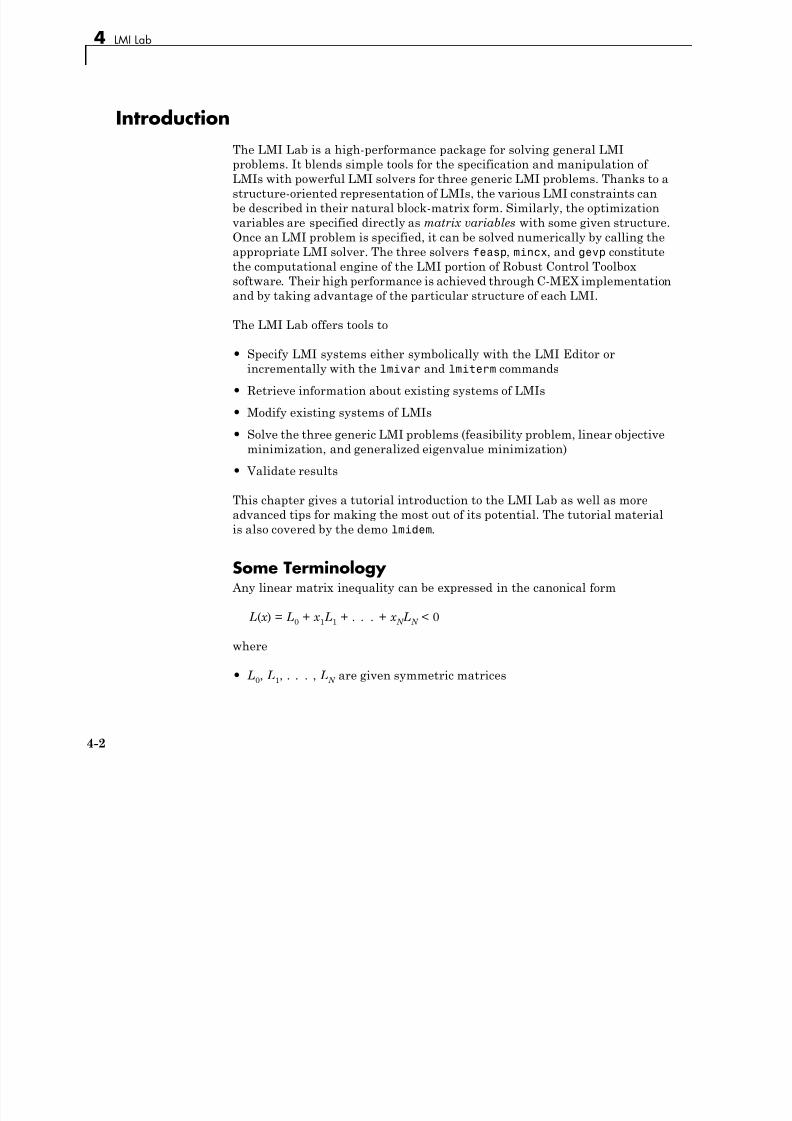
7/30/2019 Robust Control Toolbox User's Guide
http://slidepdf.com/reader/full/robust-control-toolbox-users-guide 102/180
p ,
be described in their natural block-matrix form. Similarly, the optimization
variables are specified directly as matrix variables with some given structure.
Once an LMI problem is specified, it can be solved numerically by calling the
appropriate LMI solver. The three solvers feasp, mincx, and gevp constitute
the computational engine of the LMI portion of Robust Control Toolboxsoftware. Their high performance is achieved through C-MEX implementation
and by taking advantage of the particular structure of each LMI.
The LMI Lab offers tools to
• Specify LMI systems either symbolically with the LMI Editor or
incrementally with the lmivar and lmiterm commands
• Retrieve information about existing systems of LMIs
• Modify existing systems of LMIs
• Solve the three generic LMI problems (feasibility problem, linear objective
minimization, and generalized eigenvalue minimization)
• Validate results
This chapter gives a tutorial introduction to the LMI Lab as well as more
advanced tips for making the most out of its potential. The tutorial material
is also covered by the demo lmidem.
Some Terminology Any linear matrix inequality can be expressed in the canonical form
L(x ) = L0
+ x 1
L1
+ . . . + x N
LN
< 0
where
• L0, L1, . . . , LN are given symmetric matrices
4-2
Introduction
• x = (x 1, . . . , x N
)T RN is the vector of scalar variables to be determined. We
refer to x 1, . . . , x N
as the decision variables. The names “design variables”
and “optimization variables” are also found in the literature.
Even though this canonical expression is generic, LMIs rarely arise in this
form in control applications. Consider for instance the Lyapunov inequality
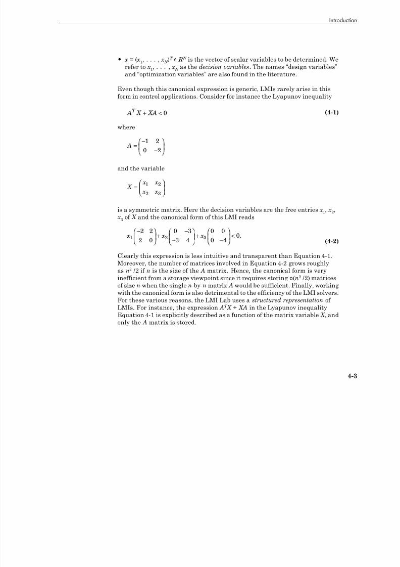
7/30/2019 Robust Control Toolbox User's Guide
http://slidepdf.com/reader/full/robust-control-toolbox-users-guide 103/180
A X XAT + < 0 (4-1)
where
A =−
−⎛
⎝ ⎜
⎞
⎠ ⎟
1 2
0 2
and the variable
X x x
x x=
⎛
⎝
⎜⎞
⎠
⎟ 1 2
2 3
is a symmetric matrix. Here the decision variables are the free entries x 1, x 2,x 3 of X and the canonical form of this LMI reads
x x x1 2 3
2 2
2 0
0 3
3 4
0 0
0 40
−⎛
⎝ ⎜
⎞
⎠ ⎟ +
−−
⎛
⎝ ⎜
⎞
⎠ ⎟ + −
⎛
⎝ ⎜
⎞
⎠ ⎟ < .
(4-2)
Clearly this expression is less intuitive and transparent than Equation 4-1.Moreover, the number of matrices involved in Equation 4-2 grows roughly
as n2 /2 if n is the size of the A matrix. Hence, the canonical form is very
inefficient from a storage viewpoint since it requires storing o(n2 /2) matrices
of size n when the single n-by-n matrix A would be sufficient. Finally, working
with the canonical form is also detrimental to the efficiency of the LMI solvers.
For these various reasons, the LMI Lab uses a structured representation of
LMIs. For instance, the expression AT X + XA in the Lyapunov inequality
Equation 4-1 is explicitly described as a function of the matrix variable X , andonly the A matrix is stored.
4-3
4 LMI Lab
In general, LMIs assume a block matrix form where each block is an affine
combination of the matrix variables. As a fairly typical illustration, consider
the following LMI drawn from H ∞
theory
N
A X XA XC B
CX I D N T
T T +−
⎛ ⎜⎜
⎞ ⎟ ⎟ < 0

7/30/2019 Robust Control Toolbox User's Guide
http://slidepdf.com/reader/full/robust-control-toolbox-users-guide 104/180
B D I T T −⎝
⎜⎜⎜
⎠
⎟ ⎟ ⎟
(4-3)
where A, B, C , D, and N are given matrices and the problem variables are X =
X T
Rn×n
and γ R. We use the following terminology to describe such LMIs:
• N is called the outer factor, and the block matrix
L X
A X XA XC B
CX I D
B D I
T T
T T
,
( ) =+
−
−
⎛
⎝
⎜⎜⎜⎜
⎞
⎠
⎟ ⎟ ⎟ ⎟
is called the inner factor. The outer factor needs not be square and is often
absent.
• X and γ are the matrix variables of the problem. Note that scalars are
considered as 1-by-1 matrices.
• The inner factor L( X, γ) is a symmetric block matrix , its block structure
being characterized by the sizes of its diagonal blocks. By symmetry, L( X,
γ) is entirely specified by the blocks on or above the diagonal.• Each block of L( X, γ) is an affine expression in the matrix variables X and
γ. This expression can be broken down into a sum of elementary terms. For
instance, the block (1,1) contains two elementary terms: AT X and XA.
• Terms are either constant or variable. Constant terms are fixed matrices
like B and D above. Variable terms involve one of the matrix variables,
like XA, XC T , and – γI above.
The LMI (Equation 4-3) is specified by the list of terms in each block, as is
any LMI regardless of its complexity.
As for the matrix variables X and γ, they are characterized by their dimensions
and structure. Common structures include rectangular unstructured,
4-4
Introduction
symmetric, skew-symmetric, and scalar. More sophisticated structures are
sometimes encountered in control problems. For instance, the matrix variable
X could be constrained to the block-diagonal structure:
X
x
x x=⎛ ⎜⎜⎜
⎞ ⎟ ⎟ ⎟
1
2 3
0 0
0 .
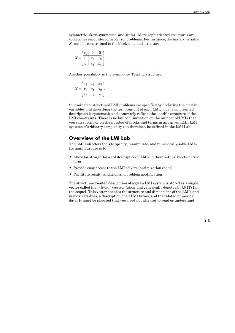
7/30/2019 Robust Control Toolbox User's Guide
http://slidepdf.com/reader/full/robust-control-toolbox-users-guide 105/180
x x⎝ ⎜⎜
⎠ ⎟⎟
3 40
Another possibility is the symmetric Toeplitz structure:
X
x x x
x x x
x x x
=⎛
⎝
⎜⎜⎜
⎞
⎠
⎟ ⎟ ⎟
1 2 3
2 1 2
3 2 1
.
Summing up, structured LMI problems are specified by declaring the matrix
variables and describing the term content of each LMI. This term-oriented
description is systematic and accurately reflects the specific structure of theLMI constraints. There is no built-in limitation on the number of LMIs that
you can specify or on the number of blocks and terms in any given LMI. LMI
systems of arbitrary complexity can therefore, be defined in the LMI Lab.
Overview of the LMI LabThe LMI Lab offers tools to specify, manipulate, and numerically solve LMIs.
Its main purpose is to
• Allow for straightforward description of LMIs in their natural block-matrix
form
• Provide easy access to the LMI solvers (optimization codes)
• Facilitate result validation and problem modification
The structure-oriented description of a given LMI system is stored as a single
vector called the internal representation and generically denoted by LMISYS inthe sequel. This vector encodes the structure and dimensions of the LMIs and
matrix variables, a description of all LMI terms, and the related numerical
data. It must be stressed that you need not attempt to read or understand
4-5
4 LMI Lab
the content of LMISYS since all manipulations involving this internal
representation can be performed in a transparent manner with LMI-Lab tools.
The LMI Lab supports the following functionalities:
Specification of a System of LMIs

7/30/2019 Robust Control Toolbox User's Guide
http://slidepdf.com/reader/full/robust-control-toolbox-users-guide 106/180
LMI systems can be either specified as symbolic matrix expressions with the
interactive graphical user interface lmiedit, or assembled incrementally with
the two commands lmivar and lmiterm. The first option is more intuitive
and transparent while the second option is more powerful and flexible.
Information RetrievalThe interactive function lmiinfo answers qualitative queries about LMI
systems created with lmiedit or lmivar and lmiterm. You can also use
lmiedit to visualize the LMI system produced by a particular sequence of
lmivar/lmiterm commands.
Solvers for LMI Optimization ProblemsGeneral-purpose LMI solvers are provided for the three generic LMI problems
defined in “Three Generic LMI Problems” on page 3-5. These solvers can
handle very general LMI systems and matrix variable structures. They return
a feasible or optimal vector of decision variables x *. The corresponding values
X X K 1* *, , of the matrix variables are given by the function dec2mat.
Result ValidationThe solution x * produced by the LMI solvers is easily validated with the
functions evallmi and showlmi. This allows a fast check and/or analysis of
the results. With evallmi, all variable terms in the LMI system are evaluated
for the value x * of the decision variables. The left and right sides of each LMI
then become constant matrices that can be displayed with showlmi.
Modification of a System of LMIs An existing system of LMIs can be modified in two ways:
• An LMI can be removed from the system with dellmi.
4-6
Introduction
• A matrix variable X can be deleted using delmvar. It can also be
instantiated, that is, set to some given matrix value. This operation is
performed by setmvar and allows, for example, to fix some variables andsolve the LMI problem with respect to the remaining ones.

7/30/2019 Robust Control Toolbox User's Guide
http://slidepdf.com/reader/full/robust-control-toolbox-users-guide 107/180
4-7
4 LMI Lab
Specifying a System of LMIs
The LMI Lab can handle any system of LMIs of the form
N T L( X 1, . . . , X K ) N < MT R( X 1, . . . , X
K ) M
where
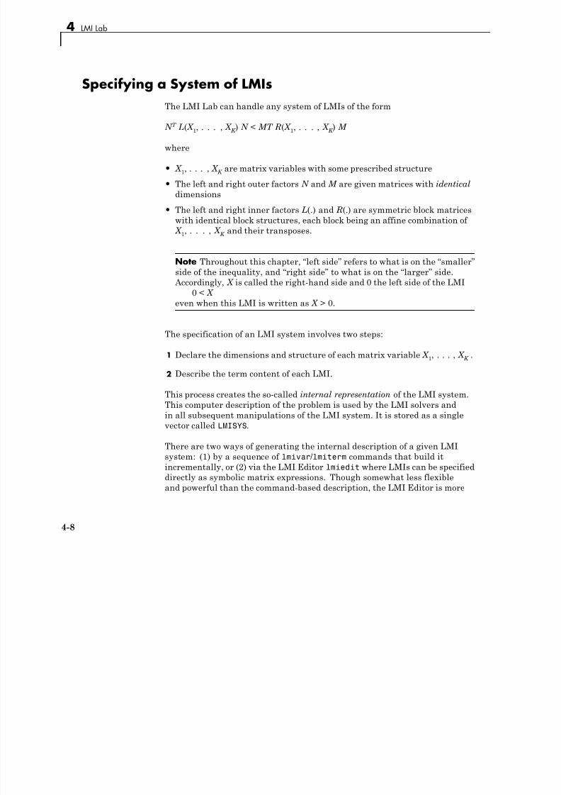
7/30/2019 Robust Control Toolbox User's Guide
http://slidepdf.com/reader/full/robust-control-toolbox-users-guide 108/180
where
• X 1, . . . , X K are matrix variables with some prescribed structure
• The left and right outer factors N and M are given matrices with identical
dimensions
• The left and right inner factors L(.) and R(.) are symmetric block matrices
with identical block structures, each block being an affine combination of X 1, . . . , X
K and their transposes.
Note Throughout this chapter, “left side” refers to what is on the “smaller”
side of the inequality, and “right side” to what is on the “larger” side. Accordingly, X is called the right-hand side and 0 the left side of the LMI
0 < X
even when this LMI is written as X > 0.
The specification of an LMI system involves two steps:
1 Declare the dimensions and structure of each matrix variable X 1
, . . . , X K
.
2 Describe the term content of each LMI.
This process creates the so-called internal representation of the LMI system.
This computer description of the problem is used by the LMI solvers and
in all subsequent manipulations of the LMI system. It is stored as a single
vector called LMISYS.
There are two ways of generating the internal description of a given LMIsystem: (1) by a sequence of lmivar/lmiterm commands that build it
incrementally, or (2) via the LMI Editor lmiedit where LMIs can be specified
directly as symbolic matrix expressions. Though somewhat less flexible
and powerful than the command-based description, the LMI Editor is more
4-8
Specifying a System of LMIs
straightforward to use, hence particularly well-suited for beginners. Thanks
to its coding and decoding capabilities, it also constitutes a good tutorial
introduction to lmivar and lmiterm. Accordingly, beginners may elect to skipthe subsections on lmivar and lmiterm and to concentrate on the GUI-based
specification of LMIs with lmiedit.
A Simple Example
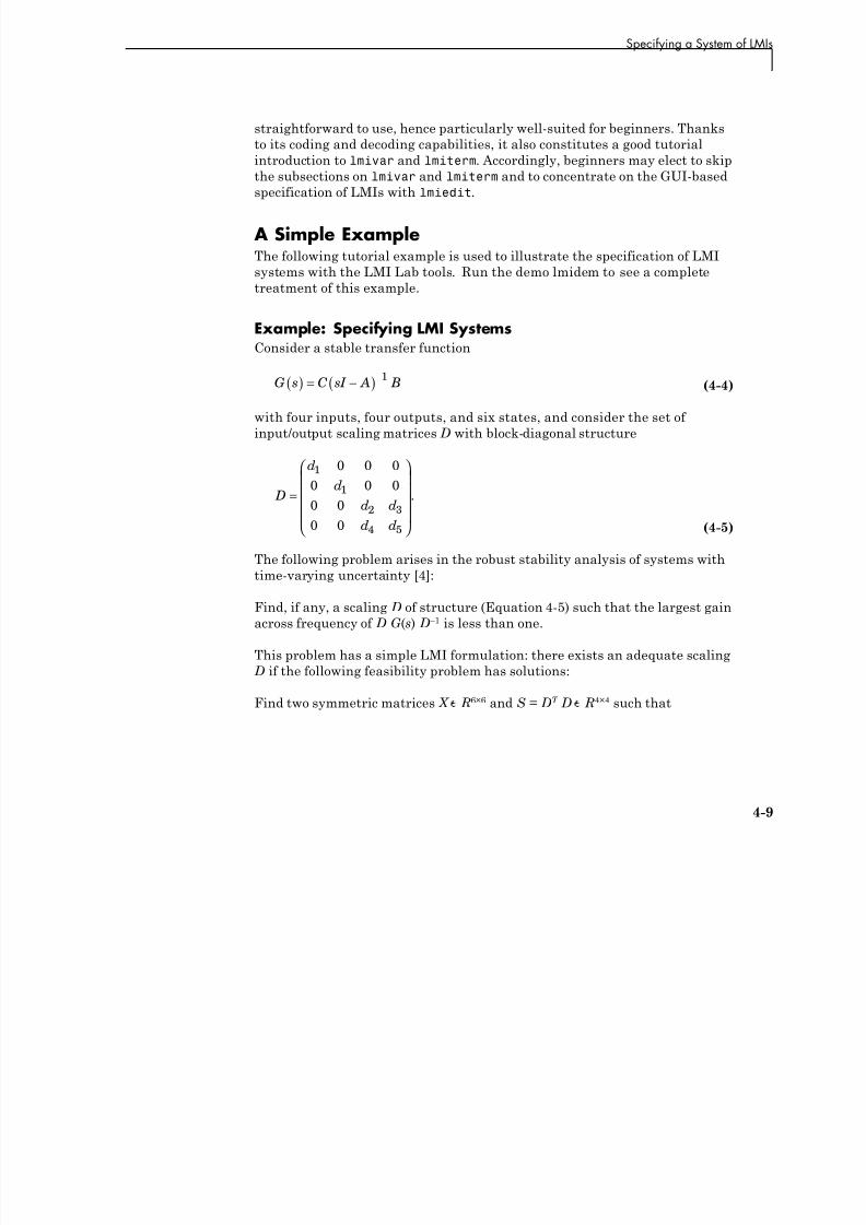
7/30/2019 Robust Control Toolbox User's Guide
http://slidepdf.com/reader/full/robust-control-toolbox-users-guide 109/180
A Simple ExampleThe following tutorial example is used to illustrate the specification of LMI
systems with the LMI Lab tools. Run the demo lmidem to see a complete
treatment of this example.
Example: Specifying LMI SystemsConsider a stable transfer function
G s C sI A B( ) = −( )−1
(4-4)
with four inputs, four outputs, and six states, and consider the set of
input/output scaling matrices D with block-diagonal structure
D
d
d
d d
d d
=
⎛
⎝
⎜⎜⎜⎜
⎞
⎠
⎟ ⎟ ⎟ ⎟
1
1
2 3
4 5
0 0 0
0 0 0
0 0
0 0
.
(4-5)
The following problem arises in the robust stability analysis of systems withtime-varying uncertainty [4]:
Find, if any, a scaling D of structure (Equation 4-5) such that the largest gain
across frequency of D G(s) D –1 is less than one.
This problem has a simple LMI formulation: there exists an adequate scaling D if the following feasibility problem has solutions:
Find two symmetric matrices X R6×6 and S = DT D R4×4 such that
4-9
4 LMI Lab
A X XA C SC XB
B X S
T T
T
+ +
−
⎛
⎝
⎜⎜
⎞
⎠
⎟ ⎟
< 0
(4-6)
X > 0 (4-7)
S > 1. (4-8)

7/30/2019 Robust Control Toolbox User's Guide
http://slidepdf.com/reader/full/robust-control-toolbox-users-guide 110/180
The LMI system (Equation 4-6, Equation 4-7, and Equation 4-8) can be
described with the LMI Editor as outlined below. Alternatively, its internal
description can be generated with lmivar and lmiterm commands as follows:
setlmis([])
X=lmivar(1,[6 1])
S=lmivar(1,[2 0;2 1])
% 1st LMI
lmiterm([1 1 1 X],1,A,'s')
lmiterm([1 1 1 S],C',C)
lmiterm([1 1 2 X],1,B)lmiterm([1 2 2 S], 1,1)
% 2nd LMI
lmiterm([ 2 1 1 X],1,1)
% 3rd LMI
lmiterm([ 3 1 1 S],1,1)
lmiterm([3 1 1 0],1)
LMISYS = getlmis
Here the lmivar commands define the two matrix variables X and S while the
lmiterm commands describe the various terms in each LMI. Upon completion,
getlmis returns the internal representation LMISYS of this LMI system. The
following subsections give more details on the syntax and usage of these
various commands:
• “Initializing the LMI System” on page 4-11
• “Specifying the LMI Variables” on page 4-11
4-10
Specifying a System of LMIs
• “Specifying Individual LMIs” on page 4-13
More information on how the internal representation is updated bylmivar/lmiterm can also be found in “How It All Works” on page 4-19.
Initializing the LMI SystemTh d i ti f LMI t h ld b i ith tl i d d ith
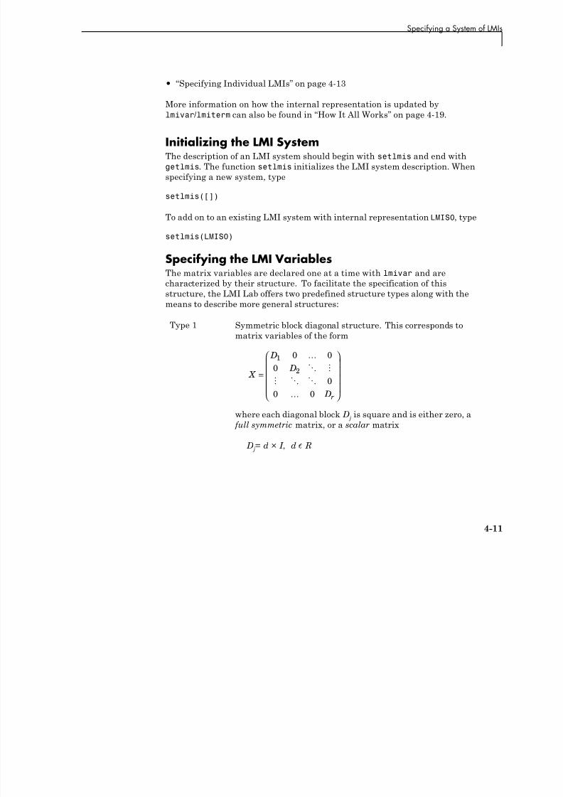
7/30/2019 Robust Control Toolbox User's Guide
http://slidepdf.com/reader/full/robust-control-toolbox-users-guide 111/180
The description of an LMI system should begin with setlmis and end with
getlmis. The function setlmis initializes the LMI system description. When
specifying a new system, type
setlmis([])
To add on to an existing LMI system with internal representation LMIS0, type
setlmis(LMIS0)
Specifying the LMI Variables
The matrix variables are declared one at a time with lmivar and arecharacterized by their structure. To facilitate the specification of this
structure, the LMI Lab offers two predefined structure types along with the
means to describe more general structures:
Type 1 Symmetric block diagonal structure. This corresponds to
matrix variables of the form
X
D
D
Dr
=
⎛
⎝
⎜⎜⎜⎜
⎞
⎠
⎟ ⎟ ⎟ ⎟
1
2
0 0
0
0
0 0
where each diagonal block D j
is square and is either zero, a full symmetric matrix, or a scalar matrix
D j= d × I , d R
4-11
4 LMI Lab
This type encompasses ordinary symmetric matrices (single
block) and scalar variables (one block of size one).Type 2 Rectangular structure. This corresponds to arbitrary
rectangular matrices without any particular structure.
Type 3 General structures. This third type is used to describe
more sophisticated structures and/or correlations between
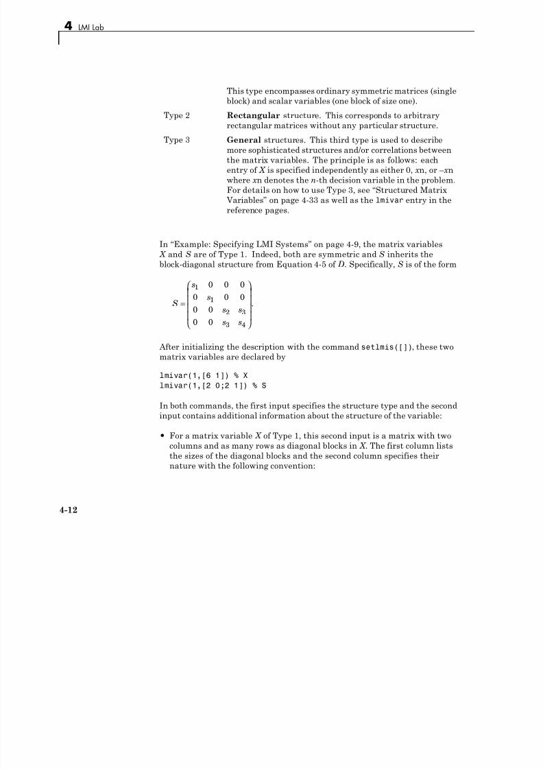
7/30/2019 Robust Control Toolbox User's Guide
http://slidepdf.com/reader/full/robust-control-toolbox-users-guide 112/180
more sophisticated structures and/or correlations between
the matrix variables. The principle is as follows: each
entry of X is specified independently as either 0, x n, or – x n
where x n denotes the n-th decision variable in the problem.
For details on how to use Type 3, see “Structured Matrix
Variables” on page 4-33 as well as the lmivar entry in the
reference pages.
In “Example: Specifying LMI Systems” on page 4-9, the matrix variables X and S are of Type 1. Indeed, both are symmetric and S inherits the
block-diagonal structure from Equation 4-5 of D. Specifically, S is of the form
S
s
s
s s
s s
=
⎛
⎝
⎜⎜⎜⎜
⎞
⎠
⎟ ⎟ ⎟ ⎟
1
1
2 3
3 4
0 0 0
0 0 0
0 0
0 0
.
After initializing the description with the command setlmis([]), these twomatrix variables are declared by
lmivar(1,[6 1]) % X
lmivar(1,[2 0;2 1]) % S
In both commands, the first input specifies the structure type and the second
input contains additional information about the structure of the variable:
• For a matrix variable X of Type 1, this second input is a matrix with two
columns and as many rows as diagonal blocks in X . The first column lists
the sizes of the diagonal blocks and the second column specifies their
nature with the following convention:
4-12
Specifying a System of LMIs
1: full symmetric block
0: scalar block
–1: zero block
In the second command, for instance,[2 0;2 1] means that S has two
diagonal blocks, the first one being a 2-by-2 scalar block and the second
one a 2-by-2 full block.
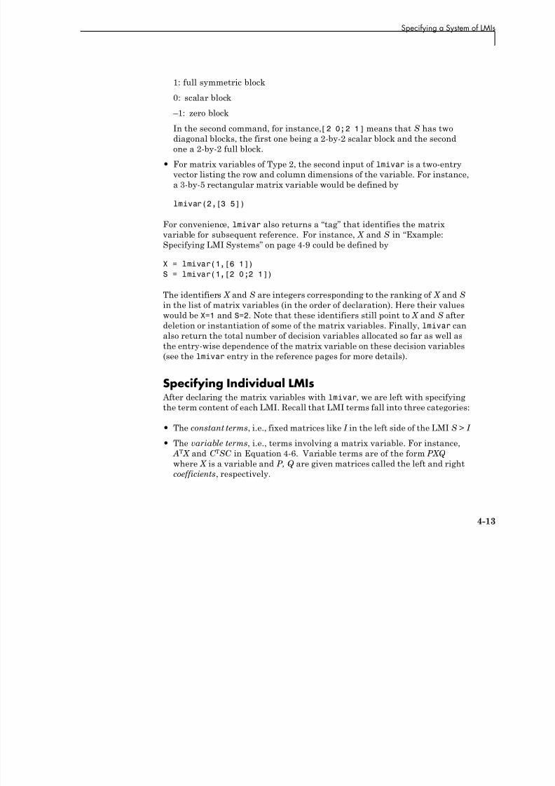
7/30/2019 Robust Control Toolbox User's Guide
http://slidepdf.com/reader/full/robust-control-toolbox-users-guide 113/180
• For matrix variables of Type 2, the second input of lmivar is a two-entry
vector listing the row and column dimensions of the variable. For instance,
a 3-by-5 rectangular matrix variable would be defined by
lmivar(2,[3 5])
For convenience, lmivar also returns a “tag” that identifies the matrix
variable for subsequent reference. For instance, X and S in “Example:
Specifying LMI Systems” on page 4-9 could be defined by
X = lmivar(1,[6 1])
S = lmivar(1,[2 0;2 1])
The identifiers X and S are integers corresponding to the ranking of X and S
in the list of matrix variables (in the order of declaration). Here their values
would be X=1 and S=2. Note that these identifiers still point to X and S after
deletion or instantiation of some of the matrix variables. Finally, lmivar can
also return the total number of decision variables allocated so far as well as
the entry-wise dependence of the matrix variable on these decision variables
(see the lmivar entry in the reference pages for more details).
Specifying Individual LMIs After declaring the matrix variables with lmivar, we are left with specifying
the term content of each LMI. Recall that LMI terms fall into three categories:
• The constant terms, i.e., fixed matrices like I in the left side of the LMI S > I
• The variable terms, i.e., terms involving a matrix variable. For instance, AT X and C TSC in Equation 4-6. Variable terms are of the form PXQ
where X is a variable and P, Q are given matrices called the left and rightcoefficients, respectively.
4-13
4 LMI Lab
• The outer factors
The following rule should be kept in mind when describing the term contentof an LMI:
Note Specify only the terms in the blocks on or above the diagonal. The
inner factors being symmetric, this is sufficient to specify the entire LMI.

7/30/2019 Robust Control Toolbox User's Guide
http://slidepdf.com/reader/full/robust-control-toolbox-users-guide 114/180
inner factors being symmetric, this is sufficient to specify the entire LMI.
Specifying all blocks results in the duplication of off-diagonal terms, hence in
the creation of a different LMI. Alternatively, you can describe the blocks on
or below the diagonal.
LMI terms are specified one at a time with lmiterm. For instance, the LMI
A X XA C SC XB
B X S
T T
T
+ +
−
⎛
⎝ ⎜⎜
⎞
⎠ ⎟ ⎟
< 0
is described by
lmiterm([1 1 1 1],1,A,'s')
lmiterm([1 1 1 2],C',C)
lmiterm([1 1 2 1],1,B)
lmiterm([1 2 2 2], 1,1)
These commands successively declare the terms AT X + XA, C T SC , XB, and
– S . In each command, the first argument is a four-entry vector listing theterm characteristics as follows:
• The first entry indicates to which LMI the term belongs. The value m means
“left side of the m-th LMI,” and −m means “right side of the m-th LMI.”
• The second and third entries identify the block to which the term belongs.
For instance, the vector [1 1 2 1] indicates that the term is attached to
the (1, 2) block.
• The last entry indicates which matrix variable is involved in the term.
This entry is 0 for constant terms, k for terms involving the k-th matrix
4-14
Specifying a System of LMIs
variable X k, and −k for terms involving X k
T (here X and S are first and
second variables in the order of declaration).
Finally, the second and third arguments of lmiterm contain the numerical
data (values of the constant term, outer factor, or matrix coefficients P and
Q for variable terms PXQ or PX T Q ). These arguments must refer to existing
MATLAB variables and be real-valued. See “Complex-Valued LMIs” on page
f h ifi i f LMI i h l l d ffi i

7/30/2019 Robust Control Toolbox User's Guide
http://slidepdf.com/reader/full/robust-control-toolbox-users-guide 115/180
4-35 for the specification of LMIs with complex-valued coefficients.
Some shorthand is provided to simplify term specification. First, blocks
are zero by default. Second, in diagonal blocks the extra argument 's'allows you to specify the conjugated expression AXB + BT X T AT with a single
lmiterm command. For instance, the first command specifies AT X + XA as the
“symmetrization” of XA. Finally, scalar values are allowed as shorthand for
scalar matrices, i.e., matrices of the form αI with α scalar. Thus, a constant
term of the form αI can be specified as the “scalar” α. This also applies to the
coefficients P and Q of variable terms. The dimensions of scalar matrices are
inferred from the context and set to 1 by default. For instance, the third LMI
S > I in “Example: Specifying Matrix Variable Structures” on page 4-33 isdescribed by
lmiterm([ 3 1 1 2],1,1) % 1*S*1 = S
lmiterm([3 1 1 0],1) % 1*I = I
Recall that by convention S is considered as the right side of the inequality,
which justifies the –3 in the first command.
Finally, to improve readability it is often convenient to attach an identifier
(tag) to each LMI and matrix variable. The variable identifiers are returned
by lmivar and the LMI identifiers are set by the function newlmi. Theseidentifiers can be used in lmiterm commands to refer to a given LMI ormatrix variable. For the LMI system of “Example: Specifying LMI Systems”
on page 4-9, this would look like:
setlmis([])
X = lmivar(1,[6 1])S = lmivar(1,[2 0;2 1])
BRL = newlmi
lmiterm([BRL 1 1 X],1,A,'s')
4-15
4 LMI Lab
lmiterm([BRL 1 1 S],C',C)
lmiterm([BRL 1 2 X],1,B)
lmiterm([BRL 2 2 S], 1,1)
Xpos = newlmi
lmiterm([-Xpos 1 1 X],1,1)
Slmi = newlmi
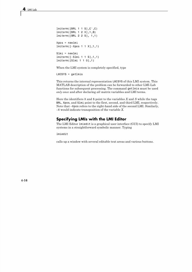
7/30/2019 Robust Control Toolbox User's Guide
http://slidepdf.com/reader/full/robust-control-toolbox-users-guide 116/180
lmiterm([-Slmi 1 1 S],1,1)
lmiterm([Slmi 1 1 0],1)
When the LMI system is completely specified, type
LMISYS = getlmis
This returns the internal representation LMISYS of this LMI system. This
MATLAB description of the problem can be forwarded to other LMI-Lab
functions for subsequent processing. The command getlmis must be usedonly once and after declaring all matrix variables and LMI terms.
Here the identifiers X and S point to the variables X and S while the tags
BRL, Xpos, and Slmi point to the first, second, and third LMI, respectively.
Note that – Xpos refers to the right-hand side of the second LMI. Similarly,
– X would indicate transposition of the variable X .
Specifying LMIs with the LMI Editor
The LMI Editor lmiedit is a graphical user interface (GUI) to specify LMIsystems in a straightforward symbolic manner. Typing
lmiedit
calls up a window with several editable text areas and various buttons.
4-16
Specifying a System of LMIs

7/30/2019 Robust Control Toolbox User's Guide
http://slidepdf.com/reader/full/robust-control-toolbox-users-guide 117/180
In more detail, to specify your LMI system,
1 Declare each matrix variable (name and structure) in the upper half of the
worksheet. The structure is characterized by its type (S for symmetric
block diagonal, R for unstructured, and G for other structures) and by an
additional “ structure” matrix. This matrix contains specific information
about the structure and corresponds to the second argument of lmivar (see
“Specifying the LMI Variables” on page 4-11 for details).
Please use one line per matrix variable in the text editing areas.
2 Specify the LMIs as MATLAB expressions in the lower half of the
worksheet. For instance, the LMI
4-17
4 LMI Lab
A X XA XB
B X I
T
T
+
−
⎛
⎝
⎜⎜
⎞
⎠
⎟ ⎟
< 0
is entered by typing
[a'*x+x*a x*b; b'*x 1] < 0
if i th i t th t i i bl X i th h lf f th

7/30/2019 Robust Control Toolbox User's Guide
http://slidepdf.com/reader/full/robust-control-toolbox-users-guide 118/180
if x is the name given to the matrix variable X in the upper half of the
worksheet. The left- and right-hand sides of the LMIs should be valid
MATLAB expressions.
Once the LMI system is fully specified, the following tasks can be performed
by clicking the corresponding button:
• Visualize the sequence of lmivar/lmiterm commands needed to describe
this LMI system (view commands button). Conversely, the LMI system
defined by a particular sequence of lmivar/lmiterm commands can be
displayed as a MATLAB expression by clicking on the describe... buttons.
Beginners can use this facility as a tutorial introduction to the lmivar and
lmiterm commands.
• Save the symbolic description of the LMI system as a MATLAB string
(save button). This description can be reloaded later on by clicking theload button.
• Read a sequence of lmivar/lmiterm commands from a file (read button).
You can then click on describe the matrix variables or describe the
LMIs to visualize the symbolic expression of the LMI system specified by
these commands. The file should describe a single LMI system but may
otherwise contain any sequence of MATLAB commands.
This feature is useful for code validation and debugging.
Write in a file the sequence of lmivar/lmiterm commands needed to
describe a particular LMI system (write button).
This is helpful to develop code and prototype MATLAB functions basedon the LMI Lab.
• Generate the internal representation of the LMI system by clicking create.
The result is written in a MATLAB variable named after the LMI system (if
4-18
Specifying a System of LMIs
the “name of the LMI system” is set to mylmi, the internal representation is
written in the MATLAB variable mylmi). Note that all LMI-related data
should be defined in the MATLAB workspace at this stage.
The internal representation can be passed directly to the LMI solvers or
any other LMI Lab function.
Keyboard Shortcuts
7/30/2019 Robust Control Toolbox User's Guide
http://slidepdf.com/reader/full/robust-control-toolbox-users-guide 119/180
As with lmiterm, you can use various shortcuts when entering LMI
expressions at the keyboard. For instance, zero blocks can be entered simply
as 0 and need not be dimensioned. Similarly, the identity matrix can beentered as 1 without dimensioning. Finally, upper diagonal LMI blocks need
not be fully specified. Rather, you can just type (*) in place of each such block.
LimitationsThough fairly general, lmiedit is not as flexible as lmiterm and the following
limitations should be kept in mind:
• Parentheses cannot be used around matrix variables. For instance, theexpression
(a*x+b)'*c + c'*(a*x+b)
is invalid when x is a variable name. By contrast,
(a+b)'*x + x'*(a+b)
is perfectly valid.
• Loops and if statements are ignored.
• When turning lmiterm commands into a symbolic description of the LMI
system, an error is issued if the first argument of lmiterm cannot be
evaluated. Use the LMI and variable identifiers supplied by newlmi and
lmivar to avoid such difficulties.
How It All WorksUsers familiar with MATLAB may wonder how lmivar and lmiterm
physically update the internal representation LMISYS since LMISYS is not
an argument to these functions. In fact, all updating is performed through
4-19
4 LMI Lab
global variables for maximum speed. These global variables are initialized
by setlmis, cleared by getlmis, and are not visible in the workspace. Even
though this artifact is transparent from the user’s viewpoint, be sure to
• Invoke getlmis only once and after completely specifying the LMI system
• Refrain from using the command clear global before the LMI system
description is ended with getlmis

7/30/2019 Robust Control Toolbox User's Guide
http://slidepdf.com/reader/full/robust-control-toolbox-users-guide 120/180
4-20
Querying the LMI System Description
Querying the LMI System Description
Recall that the full description of an LMI system is stored as a single vectorcalled the internal representation. The user should not attempt to read
or retrieve information directly from this vector. Robust Control Toolbox
software provides three functions called lmiinfo, lminbr, and matnbr to
extract and display all relevant information in a user-readable format.

7/30/2019 Robust Control Toolbox User's Guide
http://slidepdf.com/reader/full/robust-control-toolbox-users-guide 121/180
lmiinfolminbr is an interactive facility to retrieve qualitative information about
LMI systems. This includes the number of LMIs, the number of matrix
variables and their structure, the term content of each LMI block, etc. To
invoke lmiinfo, enter
lmiinfo(LMISYS)
where LMISYS is the internal representation of the LMI system produced
by getlmis.
lminbr and matnbrThese two functions return the number of LMIs and the number of matrix
variables in the system. To get the number of matrix variables, for instance,
enter
matnbr(LMISYS)
4-21
4 LMI Lab
LMI Solvers
LMI solvers are provided for the following three generic optimizationproblems (here x denotes the vector of decision variables, i.e., of the free
entries of the matrix variables X 1, . . . , X K
):
• Feasibility problem
Find x RN (or equivalently matrices X 1, . . . , X K with prescribed structure)

7/30/2019 Robust Control Toolbox User's Guide
http://slidepdf.com/reader/full/robust-control-toolbox-users-guide 122/180
that satisfies the LMI system
A(x ) < B(x )
The corresponding solver is called feasp.
• Minimization of a linear objective under LMI constraints
Minimize cT x over x RN subject to A(x ) < B(x )
The corresponding solver is called mincx.
• Generalized eigenvalue minimization problem
Minimize λ over x RN subject to
C (x ) < D(x )
0 < B(x )
A(x ) < λ B(x ).
The corresponding solver is called gevp.
Note that A(x ) < B(x ) above is a shorthand notation for general structuredLMI systems with decision variables x = (x 1, . . . , x
N ).
The three LMI solvers feasp, mincx, and gevp take as input the internal
representation LMISYS of an LMI system and return a feasible or optimizing
value x * of the decision variables. The corresponding values of the matrix
variables X 1, . . . , X K are derived from x * with the function dec2mat. These
solvers are C-MEX implementations of the polynomial-time Projective
Algorithm Projective Algorithm of Nesterov and Nemirovski [3], [2].
For generalized eigenvalue minimization problems, it is necessary to
distinguish between the standard LMI constraints C(x ) < D(x ) and the
linear-fractional LMIs
4-22
LMI Solvers
A(x) < λB(x)
attached to the minimization of the generalized eigenvalue λ. When using
gevp, you should follow these three rules to ensure proper specification of
the problem:
• Specify the LMIs involving λ as A(x ) < B(x ) (without the λ)
• Specify them last in the LMI system. gevp systematically assumes that the
last L LMIs are linear fractional if L is the number of LMIs involving λ
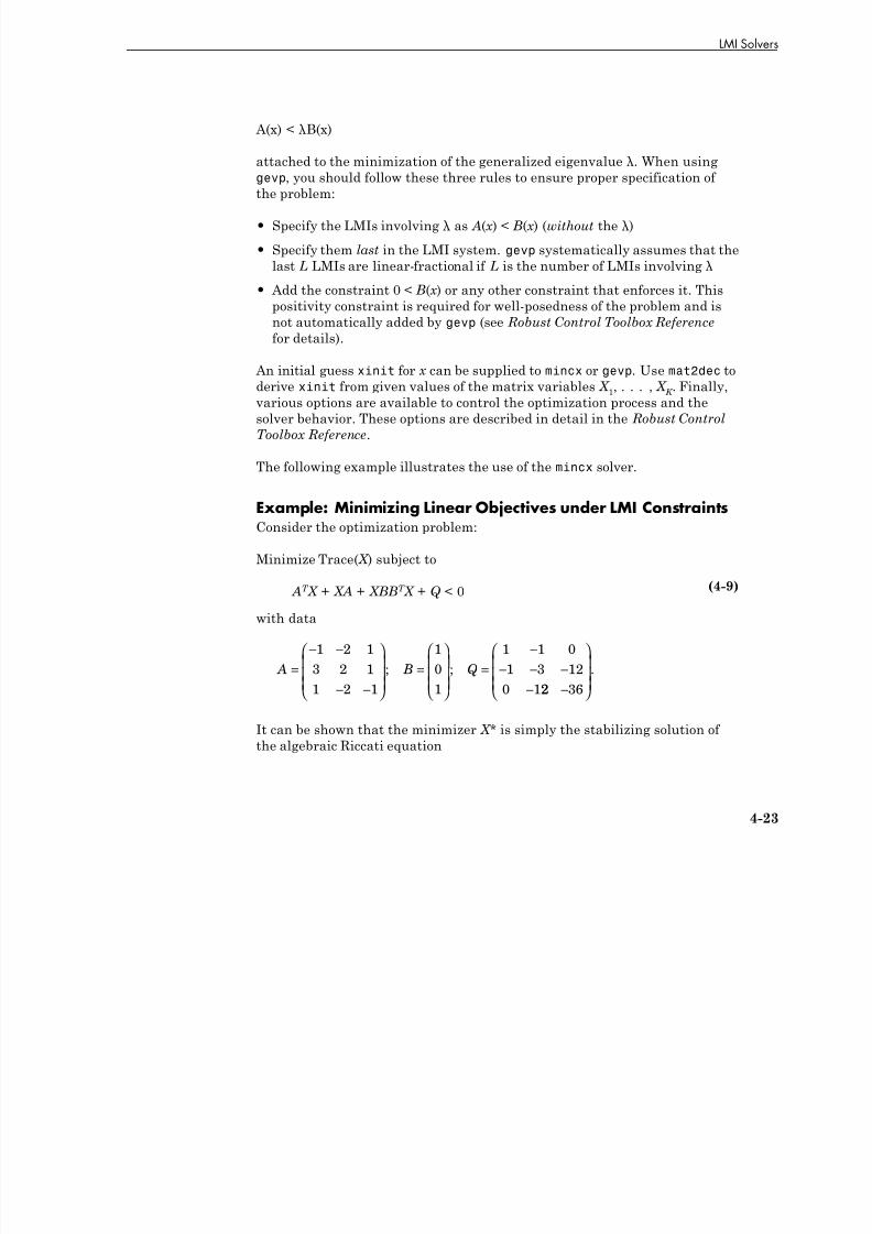
7/30/2019 Robust Control Toolbox User's Guide
http://slidepdf.com/reader/full/robust-control-toolbox-users-guide 123/180
last L LMIs are linear-fractional if L is the number of LMIs involving λ
• Add the constraint 0 < B(x ) or any other constraint that enforces it. This
positivity constraint is required for well-posedness of the problem and isnot automatically added by gevp (see Robust Control Toolbox Reference
for details).
An initial guess xinit for x can be supplied to mincx or gevp. Use mat2dec to
derive xinit from given values of the matrix variables X 1, . . . , X K
. Finally,
various options are available to control the optimization process and the
solver behavior. These options are described in detail in the Robust Control
Toolbox Reference.
The following example illustrates the use of the mincx solver.
Example: Minimizing Linear Objectives under LMI ConstraintsConsider the optimization problem:
Minimize Trace( X ) subject to
AT X + XA + XBBT X + Q < 0 (4-9)
with data
A B Q=− −
− −
⎛
⎝
⎜⎜⎜
⎞
⎠
⎟ ⎟ ⎟
=⎛
⎝
⎜⎜⎜
⎞
⎠
⎟ ⎟ ⎟
=−
− − −
−
1 2 1
3 2 1
1 2 1
1
0
1
1 1 0
1 3 12
0 1
; ;
22 36−
⎛
⎝
⎜⎜⎜
⎞
⎠
⎟ ⎟ ⎟
.
It can be shown that the minimizer X * is simply the stabilizing solution of
the algebraic Riccati equation
4-23
4 LMI Lab
AT X + XA + XBBT X + Q = 0
This solution can be computed directly with the Riccati solver care and
compared to the minimizer returned by mincx.
From an LMI optimization standpoint, the problem specified in Equation 4-9
is equivalent to the following linear objective minimization problem:
Minimize Trace( X ) subject to
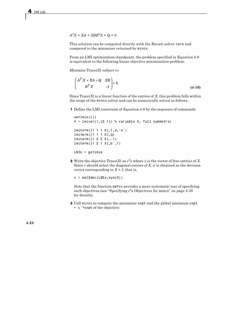
7/30/2019 Robust Control Toolbox User's Guide
http://slidepdf.com/reader/full/robust-control-toolbox-users-guide 124/180
A X XA Q XB
B X I
T
T + + −
⎛
⎝ ⎜⎜
⎞
⎠ ⎟ ⎟ < 0.
(4-10)
Since Trace( X ) is a linear function of the entries of X , this problem falls within
the scope of the mincx solver and can be numerically solved as follows:
1 Define the LMI constraint of Equation 4-9 by the sequence of commands
setlmis([])X = lmivar(1,[3 1]) % variable X, full symmetric
lmiterm([1 1 1 X],1,a,'s')
lmiterm([1 1 1 0],q)
lmiterm([1 2 2 0],-1)
lmiterm([1 2 1 X],b',1)
LMIs = getlmis
2 Write the objective Trace( X ) as cT x where x is the vector of free entries of X .
Since c should select the diagonal entries of X , it is obtained as the decision
vector corresponding to X = I , that is,
c = mat2dec(LMIs,eye(3))
Note that the function defcx provides a more systematic way of specifying
such objectives (see “Specifying cTx Objectives for mincx” on page 4-38for details).
3 Call mincx to compute the minimizer xopt and the global minimum copt
= c'*xopt of the objective:
4-24
LMI Solvers
options = [1e 5,0,0,0,0]
[copt,xopt] = mincx(LMIs,c,options)
Here 1e 5 specifies the desired relative accuracy on copt.
The following trace of the iterative optimization performed by mincx
appears on the screen:
Solver for linear objective minimization under LMI constraints
Iterations : Best objective value so far
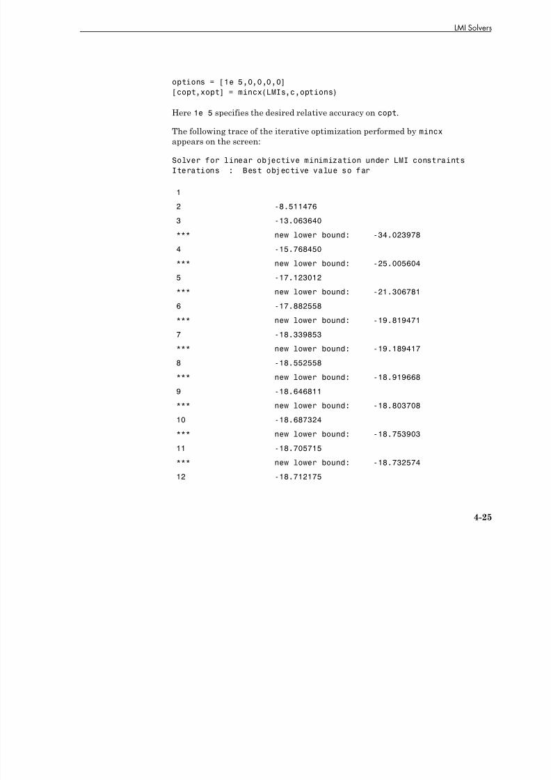
7/30/2019 Robust Control Toolbox User's Guide
http://slidepdf.com/reader/full/robust-control-toolbox-users-guide 125/180
Iterations : Best objective value so far
1
2 -8.511476
3 -13.063640
*** new lower bound: -34.023978
4 -15.768450
*** new lower bound: -25.005604
5 -17.123012
*** new lower bound: -21.306781
6 -17.882558
*** new lower bound: -19.819471
7 -18.339853
*** new lower bound: -19.189417
8 -18.552558
*** new lower bound: -18.919668
9 -18.646811
*** new lower bound: -18.803708
10 -18.687324
*** new lower bound: -18.753903
11 -18.705715
*** new lower bound: -18.732574
12 -18.712175
4-25
4 LMI Lab
*** new lower bound: -18.723491
13 -18.714880
*** new lower bound: -18.719624
14 -18.716094
*** new lower bound: -18.717986
15 -18.716509
*** new lower bound: -18.717297
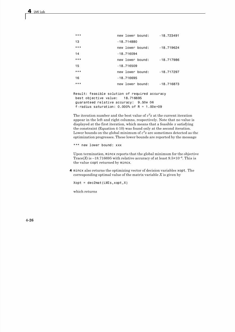
7/30/2019 Robust Control Toolbox User's Guide
http://slidepdf.com/reader/full/robust-control-toolbox-users-guide 126/180
16 -18.716695
*** new lower bound: -18.716873
Result: feasible solution of required accuracy
best objective value: 18.716695
guaranteed relative accuracy: 9.50e 06
f-radius saturation: 0.000% of R = 1.00e+09
The iteration number and the best value of cT
x at the current iterationappear in the left and right columns, respectively. Note that no value is
displayed at the first iteration, which means that a feasible x satisfying
the constraint (Equation 4-10) was found only at the second iteration.
Lower bounds on the global minimum of cT x are sometimes detected as the
optimization progresses. These lower bounds are reported by the message
*** new lower bound: xxx
Upon termination, mincx reports that the global minimum for the objective
Trace( X ) is –18.716695 with relative accuracy of at least 9.5×10 –6. This is
the value copt returned by mincx.
4 mincx also returns the optimizing vector of decision variables xopt. The
corresponding optimal value of the matrix variable X is given by
Xopt = dec2mat(LMIs,xopt,X)
which returns
4-26
LMI Solvers
X opt =− −− −
−
6 3542 5 8895 2 2046
5 8895 6 2855 2 2201
2 2046 2 2201
. . .
. . .
. . 66 0771.
.
⎛
⎝
⎜⎜
⎜
⎞
⎠
⎟ ⎟
⎟
This result can be compared with the stabilizing Riccati solution computed
by care:
Xst = care(a,b,q, 1)
norm(Xopt-Xst)
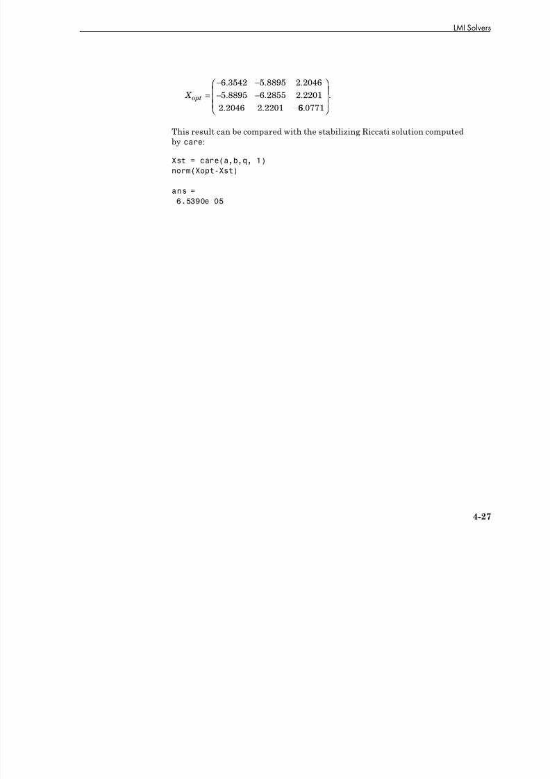
7/30/2019 Robust Control Toolbox User's Guide
http://slidepdf.com/reader/full/robust-control-toolbox-users-guide 127/180
norm(Xopt Xst)
ans =6.5390e 05
4-27
4 LMI Lab
From Decision to Matrix Variables and Vice Versa
While LMIs are specified in terms of their matrix variables X 1, . . . , X
K , the
LMI solvers optimize the vector x of free scalar entries of these matrices,
called the decision variables. The two functions mat2dec and dec2mat perform
the conversion between these two descriptions of the problem variables.
Consider an LMI system with three matrix variables X 1, X 2, X 3. Given
particular values X1, X2, X3 of these variables, the corresponding value xdec
of the vector of decision variables is returned by mat2dec:
7/30/2019 Robust Control Toolbox User's Guide
http://slidepdf.com/reader/full/robust-control-toolbox-users-guide 128/180
of the vector of decision variables is returned by mat2dec:
xdec = mat2dec(LMISYS,X1,X2,X3)
An error is issued if the number of arguments following LMISYS differs from
the number of matrix variables in the problem (see matnbr).
Conversely, given a value xdec of the vector of decision variables, the
corresponding value of the k-th matrix is given by dec2mat. For instance, the
value X2 of the second matrix variable is extracted from xdec by
X2 = dec2mat(LMISYS,xdec,2)
The last argument indicates that the second matrix variable is requested. It
could be set to the matrix variable identifier returned by lmivar.
The total numbers of matrix variables and decision variables are returned by
matnbr and decnbr, respectively. In addition, the function decinfo provides
precise information about the mapping between decision variables and matrixvariable entries (see the Robust Control Toolbox Reference).
4-28
Validating Results
Validating Results
The LMI Lab offers two functions to analyze and validate the results of
an LMI optimization. The function evallmi evaluates all variable terms
in an LMI system for a given value of the vector of decision variables, for
instance, the feasible or optimal vector returned by the LMI solvers. Once
this evaluation is performed, the left and right sides of a particular LMI are
returned by showlmi.
In the LMI problem considered in “Example: Minimizing Linear Objectives
7/30/2019 Robust Control Toolbox User's Guide
http://slidepdf.com/reader/full/robust-control-toolbox-users-guide 129/180
In the LMI problem considered in Example: Minimizing Linear Objectives
under LMI Constraints” on page 4-23, you can verify that the minimizer xopt
returned by mincx satisfies the LMI constraint (Equation 4-10) as follows:
evlmi = evallmi(LMIs,xopt)
[lhs,rhs] = showlmi(evlmi,1)
The first command evaluates the system for the value xopt of the decision
variables, and the second command returns the left and right sides of the first
(and only) LMI. The negative definiteness of this LMI is checked by
eig(lhs-rhs)
ans =
2.0387e 04
3.9333e 05
1.8917e 07
4.6680e+01
4-29
4 LMI Lab
Modifying a System of LMIs
Once specified, a system of LMIs can be modified in several ways with the
functions dellmi, delmvar, and setmvar.
Deleting an LMIThe first possibility is to remove an entire LMI from the system with dellmi.
For instance, suppose that the LMI system of “Example: Specifying LMI
Systems” on page 4-9 is described in LMISYS and that we want to remove the

7/30/2019 Robust Control Toolbox User's Guide
http://slidepdf.com/reader/full/robust-control-toolbox-users-guide 130/180
Systems on page 4 9 is described in LMISYS and that we want to remove the
positivity constraint on X . This is done by
NEWSYS = dellmi(LMISYS,2)
where the second argument specifies deletion of the second LMI. The resulting
system of two LMIs is returned in NEWSYS.
The LMI identifiers (initial ranking of the LMI in the LMI system) are not
altered by deletions. As a result, the last LMI
S > I
remains known as the third LMI even though it now ranks second in the
modified system. To avoid confusion, it is safer to refer to LMIs via the
identifiers returned by newlmi. If BRL, Xpos, and Slmi are the identifiers
attached to the three LMIs, Equation 4-6 – Equation 4-8, Slmi keeps pointing
to S > I even after deleting the second LMI by
NEWSYS = dellmi(LMISYS,Xpos)
Deleting a Matrix Variable Another way of modifying an LMI system is to delete a matrix variable, that
is, to remove all variable terms involving this matrix variable. This operation
is performed by delmvar. For instance, consider the LMI
AT X + XA + BW + W T BT + I < 0
with variables X = X T R4×4 and W R2×4. This LMI is defined by
setlmis([])
4-30
Modifying a System of LMIs
X = lmivar(1,[4 1]) % X
W = lmivar(2,[2 4]) % W
lmiterm([1 1 1 X],1,A,'s')lmiterm([1 1 1 W],B,1,'s')
lmiterm([1 1 1 0],1)
LMISYS = getlmis
To delete the variable W , type the command

7/30/2019 Robust Control Toolbox User's Guide
http://slidepdf.com/reader/full/robust-control-toolbox-users-guide 131/180
NEWSYS = delmvar(LMISYS,W)
The resulting NEWSYS now describes the Lyapunov inequality
AT X + XA + I < 0
Note that delmvar automatically removes all LMIs that depended only onthe deleted matrix variable.
The matrix variable identifiers are not affected by deletions and continue
to point to the same matrix variable. For subsequent manipulations, it
is therefore advisable to refer to the remaining variables through their
identifier. Finally, note that deleting a matrix variable is equivalent to setting
it to the zero matrix of the same dimensions with setmvar.
Instantiating a Matrix VariableThe function setmvar is used to set a matrix variable to some given value. As
a result, this variable is removed from the problem and all terms involving
it become constant terms. This is useful, for instance, to fixsetmvar some
variables and optimize with respect to the remaining ones.
Consider again “Example: Specifying LMI Systems” on page 4-9 and suppose
we want to know if the peak gain of G itself is less than one, that is, if
G ∞ < 1
4-31
4 LMI Lab
This amounts to setting the scaling matrix D (or equivalently, S = DT D) to
a multiple of the identity matrix. Keeping in mind the constraint S > I , a
legitimate choice is S = 2-βψ-I . To set S to this value, enter
NEWSYS = setmvar(LMISYS,S,2)
The second argument is the variable identifier S, and the third argument is
the value to which S should be set. Here the value 2 is shorthand for 2-by-I .
The resulting system NEWSYS reads
T TC⎛ ⎞
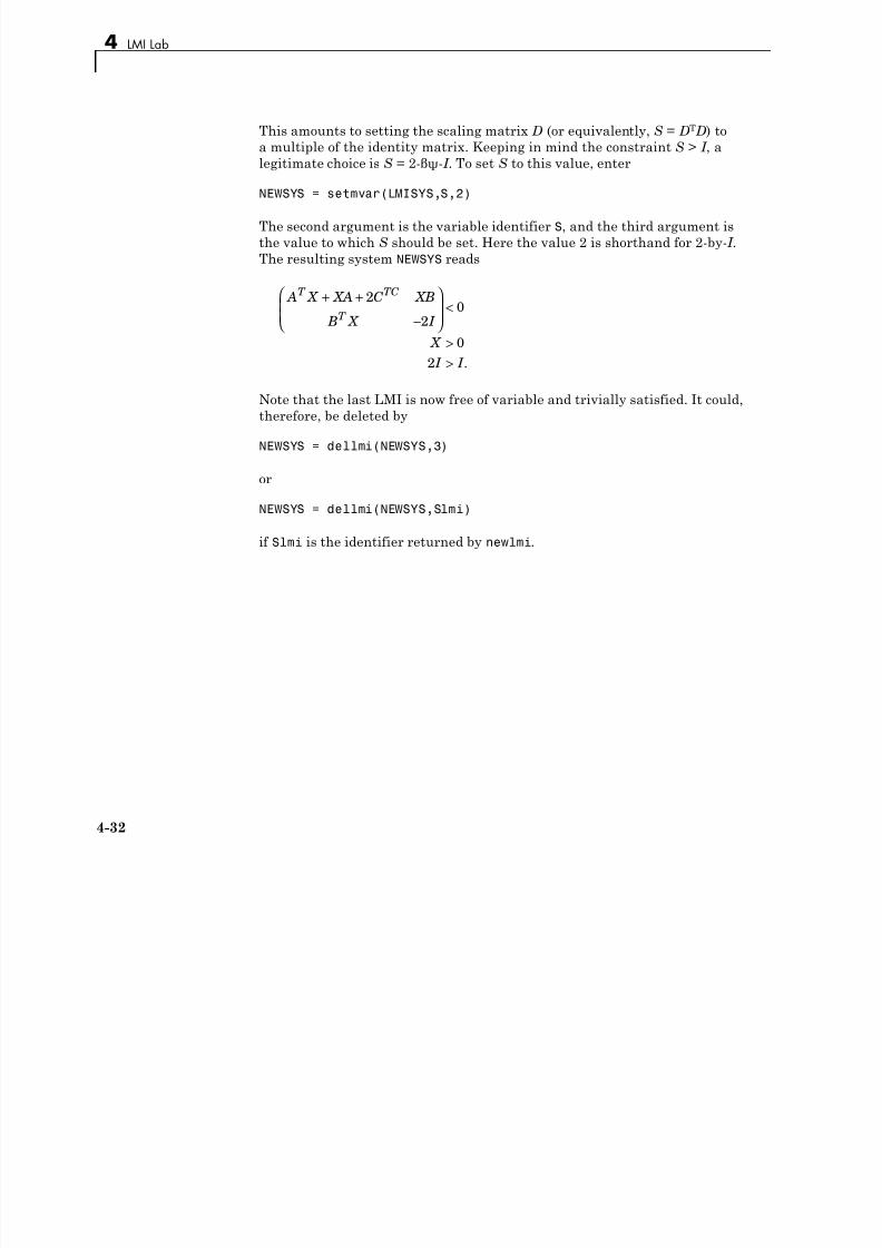
7/30/2019 Robust Control Toolbox User's Guide
http://slidepdf.com/reader/full/robust-control-toolbox-users-guide 132/180
A X XA C XB
B X I
X
I I
T TC
T
+ +
−
⎛
⎝ ⎜⎜
⎞
⎠ ⎟ ⎟ <
>>
2
20
0
2 .
Note that the last LMI is now free of variable and trivially satisfied. It could,
therefore, be deleted by
NEWSYS = dellmi(NEWSYS,3)
or
NEWSYS = dellmi(NEWSYS,Slmi)
if Slmi is the identifier returned by newlmi.
4-32
Advanced Topics
Advanced Topics
This last section gives a few hints for making the most out of the LMI Lab. It
is directed toward users who are comfortable with the basics, as described in
“Introduction” on page 4-2.
Structured Matrix VariablesFairly complex matrix variable structures and interdependencies can
be specified with lmivar. Recall that the symmetric block-diagonal or
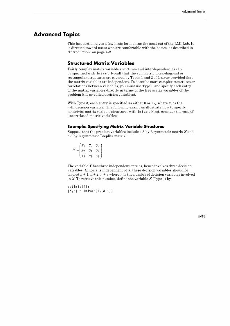
7/30/2019 Robust Control Toolbox User's Guide
http://slidepdf.com/reader/full/robust-control-toolbox-users-guide 133/180
rectangular structures are covered by Types 1 and 2 of lmivar provided that
the matrix variables are independent. To describe more complex structures orcorrelations between variables, you must use Type 3 and specify each entry
of the matrix variables directly in terms of the free scalar variables of the
problem (the so-called decision variables).
With Type 3, each entry is specified as either 0 or ±x n where x n is then-th decision variable. The following examples illustrate how to specify
nontrivial matrix variable structures with lmivar. First, consider the case of
uncorrelated matrix variables.
Example: Specifying Matrix Variable StructuresSuppose that the problem variables include a 3-by-3 symmetric matrix X and
a 3-by-3 symmetric Toeplitz matrix:
Y
y y y
y y y y y y
=
⎛
⎝ ⎜⎜⎜
⎞
⎠ ⎟ ⎟ ⎟
1 2 3
2 1 2
3 2 1
.
The variable Y has three independent entries, hence involves three decision
variables. Since Y is independent of X , these decision variables should be
labeled n + 1, n + 2, n + 3 where n is the number of decision variables involved
in X . To retrieve this number, define the variable X (Type 1) by
setlmis([])
[X,n] = lmivar(1,[3 1])
4-33
4 LMI Lab
The second output argument n gives the total number of decision variables
used so far (here n = 6). Given this number, Y can be defined by
Y = lmivar(3,n+[1 2 3;2 1 2;3 2 1])
or equivalently by
Y = lmivar(3,toeplitz(n+[1 2 3]))
where toeplitz is a standard MATLAB function. For verification purposes,
we can visualize the decision variable distributions in X and Y with decinfo:
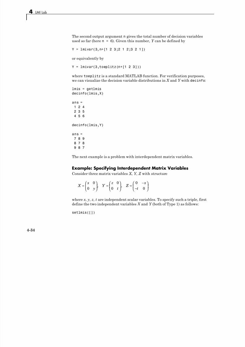
7/30/2019 Robust Control Toolbox User's Guide
http://slidepdf.com/reader/full/robust-control-toolbox-users-guide 134/180
we can visualize the decision variable distributions in X and Y with decinfo:
lmis = getlmis
decinfo(lmis,X)
ans =
1 2 4
2 3 5
4 5 6
decinfo(lmis,Y)
ans =
7 8 9
8 7 8
9 8 7
The next example is a problem with interdependent matrix variables.
Example: Specifying Interdependent Matrix VariablesConsider three matrix variables X , Y , Z with structure
X x
yY
z
t Z
x
t=
⎛
⎝ ⎜
⎞
⎠ ⎟ =
⎛
⎝ ⎜
⎞
⎠ ⎟ =
−−
⎛
⎝ ⎜
⎞
⎠ ⎟
0
0
0
0
0
0, ,
where x , y, z, t are independent scalar variables. To specify such a triple, first
define the two independent variables X and Y (both of Type 1) as follows:
setlmis([])
4-34
Advanced Topics
[X,n,sX] = lmivar(1,[1 0;1 0])
[Y,n,sY] = lmivar(1,[1 0;1 0])
The third output of lmivar gives the entry-wise dependence of X and Y on thedecision variables (x 1, x 2, x 3, x 4) := (x , y, z, t):
sX =
1 0
0 2
sY =
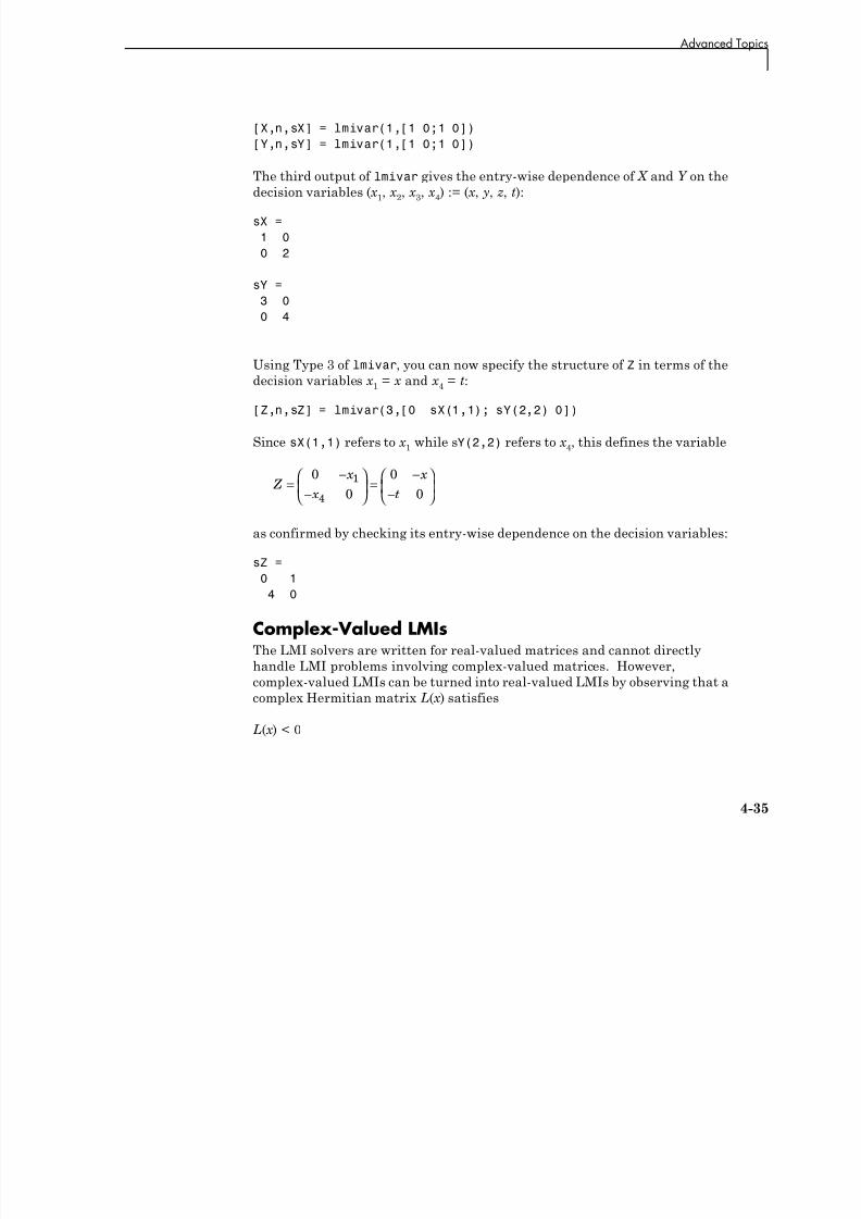
7/30/2019 Robust Control Toolbox User's Guide
http://slidepdf.com/reader/full/robust-control-toolbox-users-guide 135/180
sY
3 00 4
Using Type 3 of lmivar, you can now specify the structure of Z in terms of the
decision variables x 1 = x and x 4 = t:
[Z,n,sZ] = lmivar(3,[0 sX(1,1); sY(2,2) 0])
Since sX(1,1) refers to x 1 while sY(2,2) refers to x 4, this defines the variable
Z x
x
x
t=
−−
⎛
⎝ ⎜
⎞
⎠ ⎟ =
−−
⎛
⎝ ⎜
⎞
⎠ ⎟
0
0
0
0
1
4
as confirmed by checking its entry-wise dependence on the decision variables:
sZ =0 1
4 0
Complex-Valued LMIsThe LMI solvers are written for real-valued matrices and cannot directly
handle LMI problems involving complex-valued matrices. However,
complex-valued LMIs can be turned into real-valued LMIs by observing that a
complex Hermitian matrix L(x ) satisfies
L(x ) < 0
4-35
4 LMI Lab
if and only if
Re Im
Im Re .
L x L x
L x L x
( )( ) ( )( )− ( )( ) ( )( )
⎛
⎝ ⎜⎜⎞
⎠ ⎟ ⎟ < 0
This suggests the following systematic procedure for turning complex LMIs
into real ones:
• Decompose every complex matrix variable X as

7/30/2019 Robust Control Toolbox User's Guide
http://slidepdf.com/reader/full/robust-control-toolbox-users-guide 136/180
X = X 1
+ jX 2
where X 1 and X 2 are real
• Decompose every complex matrix coefficient A as
A = A1 + jA2
where A1 and A2 are real
• Carry out all complex matrix products. This yields affine expressions in
X 1, X 2 for the real and imaginary parts of each LMI, and an equivalentreal-valued LMI is readily derived from the above observation.
For LMIs without outer factor, a streamlined version of this procedure
consists of replacing any occurrence of the matrix variable X = X 1 + jX 2 by
X X
X X
1 2
2 1−⎛
⎝ ⎜
⎞
⎠ ⎟
and any fixed matrix A = A1 + jA2, including real ones, by
A A
A A
1 2
2 1−⎛
⎝ ⎜
⎞
⎠ ⎟ .
For instance, the real counterpart of the LMI system
M H XM < X , X = X H > I (4-11)
reads (given the decompositions M = M 1 + jM 2 and X = X 1 + jX 2 with M j, Xj
real):
4-36
Advanced Topics
M M
M M
X X
X X
M M
M M
X X
X X
T 1 2
2 1
1 2
2 1
1 2
2 1
1 2
2 1−⎛
⎝ ⎜
⎞
⎠ ⎟ −
⎛
⎝ ⎜
⎞
⎠ ⎟ −⎛
⎝ ⎜
⎞
⎠ ⎟ < −
⎛
⎝ ⎜⎜
⎞
⎠ ⎟
−⎛ ⎝ ⎜ ⎞
⎠ ⎟ <
X X
X X I
1 2
2 1
.
Note that X = X H in turn requires that X X H 1 1= and X X T
2 2 0+ = .
Consequently, X 1 and X2 should be declared as symmetric and skew-
symmetric matrix variables, respectively.

7/30/2019 Robust Control Toolbox User's Guide
http://slidepdf.com/reader/full/robust-control-toolbox-users-guide 137/180
Assuming, for instance, that M C5×5, the LMI system (Equation 4-11) wouldbe specified as follows:
M1=real(M), M2=imag(M)
bigM=[M1 M2;-M2 M1]
setlmis([])
% declare bigX=[X1 X2;-X2 X1] with X1=X1' and X2+X2'=0:
[X1,n1,sX1] = lmivar(1,[5 1])
[X2,n2,sX2] = lmivar(3,skewdec(5,n1))
bigX = lmivar(3,[sX1 sX2;-sX2 sX1])
% describe the real counterpart of (1.12):
lmiterm([1 1 1 0],1)
lmiterm([ 1 1 1 bigX],1,1)lmiterm([2 1 1 bigX],bigM',bigM)
lmiterm([ 2 1 1 bigX],1,1)
lmis = getlmis
Note the three-step declaration of the structured matrix variable bigX,
bigX X X X X = −⎛
⎝ ⎜ ⎞
⎠ ⎟ 1 2
2 1.
4-37
4 LMI Lab
1 Specify X 1 as a (real) symmetric matrix variable and save its structure
description sX1 as well as the number n1 of decision variables used in X 1.
2 Specify X 2 as a skew-symmetric matrix variable using Type 3 of lmivarand the utility skewdec. The command skewdec(5,n1) creates a 5-by–5
skew-symmetric structure depending on the decision variables n1 + 1,
n1 + 2,...
3 Define the structure of bigX in terms of the structures sX1 and sX2 of X 1and X 2.
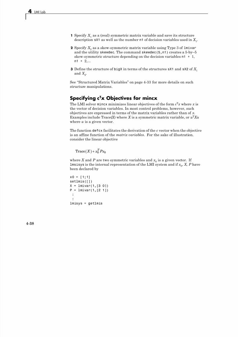
7/30/2019 Robust Control Toolbox User's Guide
http://slidepdf.com/reader/full/robust-control-toolbox-users-guide 138/180
See “Structured Matrix Variables” on page 4-33 for more details on suchstructure manipulations.
Specifying cT x Objectives for mincx The LMI solver mincx minimizes linear objectives of the form cTx where x is
the vector of decision variables. In most control problems, however, such
objectives are expressed in terms of the matrix variables rather than of x .
Examples include Trace( X ) where X is a symmetric matrix variable, or uT Xu
where u is a given vector.
The function defcx facilitates the derivation of the c vector when the objective
is an affine function of the matrix variables. For the sake of illustration,
consider the linear objective
Trace X x PxT ( ) + 0 0
where X and P are two symmetric variables and x 0 is a given vector. If
lmsisys is the internal representation of the LMI system and if x 0, X, P have
been declared by
x0 = [1;1]
setlmis([])
X = lmivar(1,[3 0])
P = lmivar(1,[2 1]):
:
lmisys = getlmis
4-38
Advanced Topics
the c vector such that c x X x PxT T = ( ) +Trace 0 0 can be computed as follows:
n = decnbr(lmisys)c = zeros(n,1)
for j=1:n,
[Xj,Pj] = defcx(lmisys,j,X,P)
c(j) = trace(Xj) + x0'*Pj*x0
end
The first command returns the number of decision variables in the problem

7/30/2019 Robust Control Toolbox User's Guide
http://slidepdf.com/reader/full/robust-control-toolbox-users-guide 139/180
The first command returns the number of decision variables in the problem
and the second command dimensions c accordingly. Then the for loop
performs the following operations:
1 Evaluate the matrix variables X and P when all entries of the decision
vector x are set to zero except xj: = 1. This operation is performed by
the function defcx. Apart from lmisys and j, the inputs of defcx are
the identifiers X and P of the variables involved in the objective, and the
outputs Xj and Pj are the corresponding values.
2 Evaluate the objective expression for X:= Xj and P:= Pj. This yields the j-th entry of c by definition.
In our example the result is
c =
3
12
1
Other objectives are handled similarly by editing the following generic
skeleton:
n = decnbr( LMI system )
c = zeros(n,1)for j=1:n,
[ matrix values ] = defcx( LMI system,j,
matrix identifiers)
c(j) = objective(matrix values)
4-39
4 LMI Lab
end
Feasibility RadiusWhen solving LMI problems with feasp, mincx, or gevp, it is possible to
constrain the solution x to lie in the ball
x T x < R2
where R > 0 is called the feasibility radius. This specifies a maximum
(Euclidean norm) magnitude for x and avoids getting solutions of very large
norm. This may also speed up computations and improve numerical stability.

7/30/2019 Robust Control Toolbox User's Guide
http://slidepdf.com/reader/full/robust-control-toolbox-users-guide 140/180
norm. This may also speed up computations and improve numerical stability.
Finally, the feasibility radius bound regularizes problems with redundant
variable sets. In rough terms, the set of scalar variables is redundant when an
equivalent problem could be formulated with a smaller number of variables.
The feasibility radius R is set by the third entry of the options vector of the
LMI solvers. Its default value is R = 109. Setting R to a negative value means
“no rigid bound,” in which case the feasibility radius is increased during the
optimization if necessary. This “flexible bound” mode may yield solutions of
large norms.
Well-Posedness IssuesThe LMI solvers used in the LMI Lab are based on interior-point optimization
techniques. To compute feasible solutions, such techniques require that the
system of LMI constraints be strictly feasible, that is, the feasible set has a
nonempty interior. As a result, these solvers may encounter difficulty when
the LMI constraints are feasible but not strictly feasible, that is, when the LMI
L(x ) ≤ 0
has solutions while
L(x ) < 0
has no solution.
For feasibility problems, this difficulty is automatically circumvented by
feasp, which reformulates the problem:
4-40
Advanced Topics
Find x such that
L(x ) ≤ 0 (4-12)
as:
Minimize t subject to
Lx < t × I . (4-13)
In this modified problem, the LMI constraint is always strictly feasible inx , t and the original LMI Equation 4-12 is feasible if and only if the global
7/30/2019 Robust Control Toolbox User's Guide
http://slidepdf.com/reader/full/robust-control-toolbox-users-guide 141/180
minimum tmin of Equation 4-12 satisfies
tmin ≤ 0
For feasible but not strictly feasible problems, however, the computational
effort is typically higher as feasp strives to approach the global optimumtmin = 0 to a high accuracy.
For the LMI problems addressed by mincx and gevp, nonstrict feasibilitygenerally causes the solvers to fail and to return an “infeasibility” diagnosis.
Although there is no universal remedy for this difficulty, it is sometimes
possible to eliminate underlying algebraic constraints to obtain a strictly
feasible problem with fewer variables.
Another issue has to do with homogeneous feasibility problems such as
AT
P + P A < 0, P > 0
While this problem is technically well-posed, the LMI optimization is likely to
produce solutions close to zero (the trivial solution of the nonstrict problem).
To compute a nontrivial Lyapunov matrix and easily differentiate between
feasibility and infeasibility, replace the constraint P > 0-by- P > αI with α > 0.
Note that this does not alter the problem due to its homogeneous nature.
Semi-Definite B(x) in gevp ProblemsConsider the generalized eigenvalue minimization problem
Minimize λ subject to
4-41
4 LMI Lab
A(x ) < λ B(x ), B(x ) > 0, C (x ) <0. (4-14)
Technically, the positivity of B(x ) for some x Rn is required for the
well-posedness of the problem and the applicability of polynomial-timeinterior-point methods. Hence problems where
B xB x
( ) =( )⎛
⎝ ⎜
⎞
⎠ ⎟
1 0
0 0
with B1(x ) > 0 strictly feasible, cannot be directly solved with gevp. A simple
remedy consists of replacing the constraints
7/30/2019 Robust Control Toolbox User's Guide
http://slidepdf.com/reader/full/robust-control-toolbox-users-guide 142/180
A(x ) < B(x ), B(x ) > 0
by
A xY
Y B x B x( ) <⎛
⎝ ⎜
⎞
⎠ ⎟ < ( ) ( ) >
0
0 001 1, ,
where Y is an additional symmetric variable of proper dimensions. The
resulting problem is equivalent to Equation 4-14 and can be solved directly
with gevp.
Efficiency and Complexity Issues As explained in “Introduction” on page 4-2, the term-oriented description
of LMIs used in the LMI Lab typically leads to higher efficiency than thecanonical representation
A0 + x 1 A1 + ... + x N A
N < 0. (4-15)
This is no longer true, however, when the number of variable terms is nearly
equal to or greater than the number N of decision variables in the problem.
If your LMI problem has few free scalar variables but many terms in each
LMI, it is therefore preferable to rewrite it as Equation 4-15 and to specify
it in this form. Each scalar variable x j is then declared independently and
the LMI terms are of the form x j A
j.
4-42
Advanced Topics
If M denotes the total row size of the LMI system and N the total number of
scalar decision variables, the flop count per iteration for the feasp and mincx
solvers is proportional to
• N 3 when the least-squares problem is solved via. Cholesly factorization
of the Hessian matrix (default) [2]
• M -by-N 2 when numerical instabilities warrant the use of QR factorization
instead
While the theory guarantees a worst-case iteration count proportional to M ,
the number of iterations actually performed grows slowly with M in most
bl Fi ll hil d bl i l i

7/30/2019 Robust Control Toolbox User's Guide
http://slidepdf.com/reader/full/robust-control-toolbox-users-guide 143/180
problems. Finally, while feasp and mincx are comparable in complexity,gevp typically demands more computational effort. Make sure that your LMI
problem cannot be solved with mincx before using gevp.
Solving M + PT XQ + QT X TP < 0In many output-feedback synthesis problems, the design can be performed
in two steps:
1 Compute a closed-loop Lyapunov function via LMI optimization.
2 Given this Lyapunov function, derive the controller state-space matrices by
solving an LMI of the form
M + P T XQ + Q T X T P < 0 (4-16)
where M , P , Q are given matrices and X is an unstructured m-by-n matrix
variable.
It turns out that a particular solution X c of Equation 4-16 can be computed
via simple linear algebra manipulations [1]. Typically, X c corresponds to the
center of the ellipsoid of matrices defined by Equation 4-16.
The function basiclmi returns the “explicit” solution X c:
Xc = basiclmi(M,P,Q)
4-43
4 LMI Lab
Since this central solution sometimes has large norm, basiclmi also offers
the option of computing an approximate least-norm solution of Equation 4-16.
This is done by
X = basiclmi(M,P,Q,'Xmin')
and involves LMI optimization to minimize X .

7/30/2019 Robust Control Toolbox User's Guide
http://slidepdf.com/reader/full/robust-control-toolbox-users-guide 144/180
4-44
Bibliography
Bibliography
[1] Gahinet, P., and P. Apkarian, “A Linear Matrix Inequality Approach to H ∞
Control,” Int. J. Robust and Nonlinear Contr., 4 (1994), pp. 421-448.
[2] Nemirovski, A., and P. Gahinet, “The Projective Method for Solving Linear
Matrix Inequalities,” Proc. Amer. Contr. Conf ., 1994, pp. 840-844.
[3] Nesterov, Yu, and A. Nemirovski, Interior Point Polynomial Methods in
Convex Programming: Theory and Applications, SIAM Books, Philadelphia,
1994.
7/30/2019 Robust Control Toolbox User's Guide
http://slidepdf.com/reader/full/robust-control-toolbox-users-guide 145/180
[4] Shamma, J.S., “Robustness Analysis for Time-Varying Systems,” Proc.
Conf. Dec. Contr., 1992, pp. 3163-3168.
4-45
4 LMI Lab

7/30/2019 Robust Control Toolbox User's Guide
http://slidepdf.com/reader/full/robust-control-toolbox-users-guide 146/180
4-46
5
Analyzing UncertaintyEffects in Simulink
“O i ” 5 2
7/30/2019 Robust Control Toolbox User's Guide
http://slidepdf.com/reader/full/robust-control-toolbox-users-guide 147/180
• “Overview” on page 5-2
• “Robust Control Toolbox Block Library” on page 5-4
• “Specifying Uncertainty Using Uncertain State Space Blocks” on page 5-5
• “Simulating Uncertainty Effects” on page 5-8
• “Computing Uncertain State-Space Models from Simulink Models” on page
5-19• “Analyzing Stability Margins” on page 5-26
5 Analyzing Uncertainty Effects in Simulink®
Overview
Robust Control Toolbox software provides tools to model uncertainty in
Simulink®. Using these tools, you can analyze how the uncertainty impactsthe time- and frequency-domain behavior of the Simulink model.
The Uncertain State Space block, included in the Robust Control Toolbox
block library, is a convenient way to incorporate uncertainty information in a
Simulink model. For more information, see “Specifying Uncertainty Using
Uncertain State Space Blocks” on page 5-5. Using this block, you can perform
the following types of analysis:
V h i d h i ff h i (M
7/30/2019 Robust Control Toolbox User's Guide
http://slidepdf.com/reader/full/robust-control-toolbox-users-guide 148/180
• Vary the uncertainty and see how it affects the time responses (Monte
Carlo analysis). See “Simulating Uncertainty Effects” on page 5-8.
• Analyze the effects of uncertainty on the linearized dynamics:
- If the operating point does not depend on the parameter uncertainty, use
ulinearize to obtain an uncertain state-space model. You can then
use usample to sample the uncertain variables and obtain a family of
LTI models.- If the operating point depends on the parameter uncertainty, use
usample to sample the uncertainty and then use the Simulink Control
Design™ linearize command to compute the linearized dynamics for
each uncertainty value.
See “How to Vary Uncertainty Values” on page 5-8 and “Working with
Models Containing Uncertain State Space Blocks” on page 5-19.
• Compute an uncertain linearization, i.e., obtain an uncertain statespace model (uss object) that combines the uncertain variables with
the linearized dynamics. You can use this model to perform worst-case
robustness analysis. See “Working with Models Containing Uncertain
State Space Blocks” on page 5-19.
If you cannot use Uncertain State Space blocks in the Simulink model because
you share the model or generate code, you can still compute an uncertain
linearization by specifying a block to linearize to an uncertain variable.For example, you can specify a gain block to linearize to an uncertain real
parameter (ureal). See “Working with Models Containing Core Simulink or
5-2
Overview
Custom Blocks” on page 5-20. You can then use the uncertain state-space
model to analyze robustness in the linear operating range.

7/30/2019 Robust Control Toolbox User's Guide
http://slidepdf.com/reader/full/robust-control-toolbox-users-guide 149/180
5-3
5 Analyzing Uncertainty Effects in Simulink®
Robust Control Toolbox Block Library
Robust Control Toolbox software provides an Uncertain State Space block to
model parametric and dynamic uncertainty in Simulink. The block libraryalso contains a MultiPlot Graph block that you use with the Uncertain State
Space block to plot and visualize Monte Carlo simulation responses.
To open the Robust Control Toolbox block library, type the following command
at the MATLAB prompt:
RCTblocks
The block library opens as shown in the following figure

7/30/2019 Robust Control Toolbox User's Guide
http://slidepdf.com/reader/full/robust-control-toolbox-users-guide 150/180
The block library opens, as shown in the following figure.
Alternatively, select Start > Simulink > Library Browser. In the Library
Browser, select Robust Control Toolbox.
For more information on the Robust Control Toolbox blocks, see Robust
Control Toolbox Reference.
5-4
Specifying Uncertainty Using Uncertain State Space Blocks
Specifying Uncertainty Using Uncertain State Space Blocks
• “How to Specify Uncertainty in Uncertain State Space Blocks” on page 5-5
• “Next Steps” on page 5-7
How to Specify Uncertainty in Uncertain State SpaceBlocksSpecifying uncertainty in the Uncertain State Space block makes the
uncertainty a part of the Simulink model and affects both simulation and
linearization. Use this approach to vary the uncertainty and analyze the
effects on simulation or linearization.
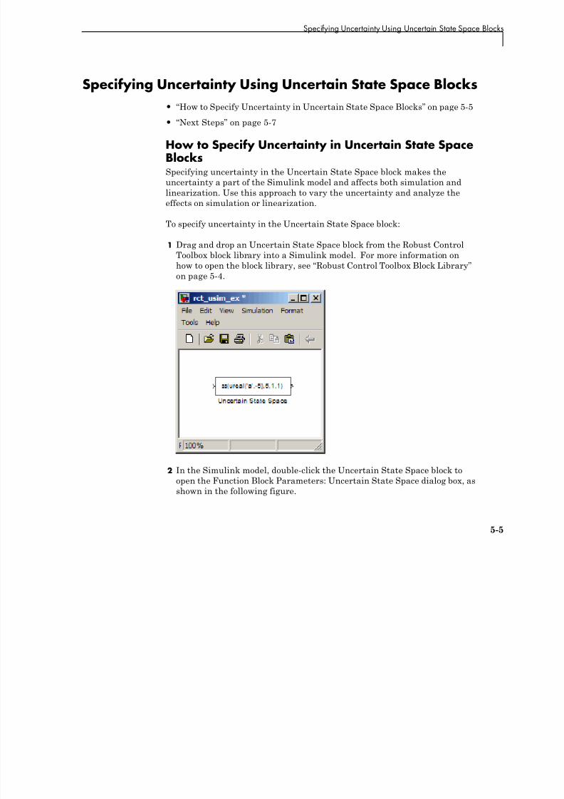
7/30/2019 Robust Control Toolbox User's Guide
http://slidepdf.com/reader/full/robust-control-toolbox-users-guide 151/180
To specify uncertainty in the Uncertain State Space block:
1 Drag and drop an Uncertain State Space block from the Robust Control
Toolbox block library into a Simulink model. For more information on
how to open the block library, see “Robust Control Toolbox Block Library”
on page 5-4.
2 In the Simulink model, double-click the Uncertain State Space block to
open the Function Block Parameters: Uncertain State Space dialog box, as
shown in the following figure.
5-5
5 Analyzing Uncertainty Effects in Simulink®

7/30/2019 Robust Control Toolbox User's Guide
http://slidepdf.com/reader/full/robust-control-toolbox-users-guide 152/180
3 Specify an uncertain state-space model in the Uncertain system variable
(uss) field. The model must be an uss object or any other model that can be
converted to uss, such as umat, ureal and ultidyn. The model depends
on a set of uncertain variables (ureal or ultidyn) and you can specify
the model as one of the following:
5-6
Specifying Uncertainty Using Uncertain State Space Blocks
• Function or expression that evaluates to an uss model. For example,
ss(ureal('a',-5),5,1,1).
• Variable, defined in the MATLAB workspace. For example, unc_sys,
where unc_sys is defined as ss(ureal('a',-5),5,1,1) in theworkspace.
4 Specify values for the uncertain variables that the uncertain state-space
model you specify in step 3 uses. For example, if you specify the uncertain
system as ureal('g',2)*tf(1,[ureal(`tau'),1], then you must specify
values for the uncertain variables g and tau. To do so, enter a structure
with fields g and tau in the Uncertainty value (struct or [] to use
nominal value) field. You can also enter [] to use the nominal values of the uncertain parameters g and tau.
7/30/2019 Robust Control Toolbox User's Guide
http://slidepdf.com/reader/full/robust-control-toolbox-users-guide 153/180
the uncertain parameters g and tau.
Tip: You can also use this field to vary the uncertainty values for
performing Monte Carlo simulation. For more information, see “Simulating
Uncertainty Effects” on page 5-8.
5 (Optional) Specify the initial states of the nominal and uncertain dynamics
in the Initial states (nominal dynamics) and Initial states (uncertain
dynamics) fields, respectively.
For more information on the block parameters, see the Uncertain State Space
block reference page.
Next Steps After you specify uncertainty in Uncertain State Space blocks, you can
perform one of the following:
• Simulate the model using nominal, manually-defined or random values, as
described in “Simulating Uncertainty Effects” on page 5-8.
• Perform an uncertain linearization, as described in “Working with
Models Containing Uncertain State Space Blocks” on page 5-19 section
of “Computing Uncertain State-Space Models from Simulink Models” on
page 5-19.
5-7
5 Analyzing Uncertainty Effects in Simulink®
Simulating Uncertainty Effects
• “How to Simulate Effects of Uncertainty” on page 5-8
• “How to Vary Uncertainty Values” on page 5-8
How to Simulate Effects of Uncertainty As described in “Specifying Uncertainty Using Uncertain State Space Blocks”
on page 5-5, the uncertain state-space model you specify in the Uncertain
State Space block depends on a set of uncertain variables (ureal or ultidyn
objects.) You can simulate the model using nominal value of these uncertain
variables. Additionally, you can sample these uncertain variables andsimulate the model for various values in the uncertainty range (Monte Carlo

7/30/2019 Robust Control Toolbox User's Guide
http://slidepdf.com/reader/full/robust-control-toolbox-users-guide 154/180
simulation.) For more information, see “How to Vary Uncertainty Values” on
page 5-8. You can view and compare the simulation results for various sample
values of uncertainty using the MultiPlot Graph block.
How to Vary Uncertainty Values
There are two ways to control the uncertainty values using the Uncertaintyvalue (struct or [] to use nominal value) field of the Uncertain State
Space block parameters dialog box:
• For simple models with few uncertain variables or one Uncertain State
Space block, type the value in the Uncertain State Space block itself. For
more information, see “Varying Uncertainty Values Using IndividualUncertain State Space Blocks” on page 5-9.
• For complex models with large number of uncertain variables or UncertainState Space blocks, use a single data structure for all uncertain variables
referenced by the model. Using this approach, you can collectively control
the values of all or a subset of uncertain variables and toggle between
nominal and user-defined values from the MATLAB prompt. For more
information, see “Varying Uncertainty Values Across Multiple Uncertain
State Space Blocks” on page 5-14.
5-8
Simulating Uncertainty Effects
Varying Uncertainty Values Using Individual Uncertain StateSpace BlocksThis section describes the workflow for varying uncertainty values using
individual Uncertain State Space blocks in a Simulink model. Use thisapproach for simple models with few uncertain variables or one Uncertain
State Space block.
This section uses a simple Simulink model to provide step-by-step instructions
for:
• Toggling between nominal, manually defined and randomly-generated
uncertainty values associated with the Uncertain State Space block.• Simulating the model’s responses for these uncertainty values

7/30/2019 Robust Control Toolbox User's Guide
http://slidepdf.com/reader/full/robust-control-toolbox-users-guide 155/180
• Simulating the model s responses for these uncertainty values.
1 Open the Simulink model rct_sim_ex1.
rct_sim_ex1
The model contains an Uncertain State Space block, as shown in the
following figure.
5-9
5 Analyzing Uncertainty Effects in Simulink®
2 Double-click the Uncertain State Space block to open the Function Block
Parameters dialog box.

7/30/2019 Robust Control Toolbox User's Guide
http://slidepdf.com/reader/full/robust-control-toolbox-users-guide 156/180
5-10
Simulating Uncertainty Effects
The Uncertain State Space block uses the uncertain system variable
unc_sys. This variable is defined in the Model workspace as unc_sys=
ss(ureal('a',-1,'Range',[-2 -.5]),1,5,0)*(1+0.1*input_unc). The
uncertain model depends on a single uncertain variable named a. TheUncertainty value field specifies to use nominal value of the uncertain
variable a.
Click OK to close the dialog box.
3 Click to simulate the model.
The software uses the nominal value of a during simulation. After the
simulation completes, the MultiPlot Graph shows the following plot.

7/30/2019 Robust Control Toolbox User's Guide
http://slidepdf.com/reader/full/robust-control-toolbox-users-guide 157/180
4 To simulate the model using a manually defined value of a:
a Double-click the Uncertain State Space block, and enter
struct('a',-0.3) in the Uncertainty value field.
5-11
5Analyzing Uncertainty Effects in Simulink®
b Click
to simulate the model.
The MultiPlot Graph shows the following responses corresponding to the

7/30/2019 Robust Control Toolbox User's Guide
http://slidepdf.com/reader/full/robust-control-toolbox-users-guide 158/180
The MultiPlot Graph shows the following responses, corresponding to the
nominal and manually-defined values of a.
5-12
Simulating Uncertainty Effects
5 Pick a random value of a in its uncertainty range. To do so, double-click the
Uncertain State Space block, and type usample(ufind(unc_sys)) in the
Uncertainty value field.
6 Analyze the uncertainty effects by simulating the model ten times usingthe following commands:
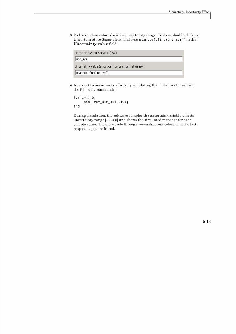
7/30/2019 Robust Control Toolbox User's Guide
http://slidepdf.com/reader/full/robust-control-toolbox-users-guide 159/180
for i=1:10;
sim('rct_sim_ex1',10);
end
During simulation, the software samples the uncertain variable a in its
uncertainty range [-2 -0.5] and shows the simulated response for eachsample value. The plots cycle through seven different colors, and the last
response appears in red.
5-13
5Analyzing Uncertainty Effects in Simulink®

7/30/2019 Robust Control Toolbox User's Guide
http://slidepdf.com/reader/full/robust-control-toolbox-users-guide 160/180
Tip: You can clear the plots in the MultiPlot Graph block before you run
the simulation.
Varying Uncertainty Values Across Multiple Uncertain StateSpace BlocksThis section describes the workflow for varying uncertainty values across
multiple Uncertain State Space blocks in a Simulink model. Use this
approach for complex models with large number of uncertain variables or
Uncertain State Space blocks.
This section uses a Simulink model to provide step-by-step instructions
for toggling between nominal and user-defined uncertainty values at the
MATLAB prompt.
1 Open the Simulink model rct_sim_ex2.
5-14
Simulating Uncertainty Effects
rct_sim_ex2
The model contains two Uncertain State Space blocks, as shown in the
following figure.

7/30/2019 Robust Control Toolbox User's Guide
http://slidepdf.com/reader/full/robust-control-toolbox-users-guide 161/180
The Unmodeled dynamics and First order with uncertain pole blocks
depend on the uncertain variables input_unc and a.
2 Double-click the Unmodeled dynamics block to open the block parameters
dialog box. The Uncertainty value field contains the variable val_all.
Similarly, the Uncertainty value field in the First order with
uncertain pole block parameters dialog contains the variable val_all. You use this variable to vary the uncertain variable values across both
the Uncertain State Space blocks.
5-15
5Analyzing Uncertainty Effects in Simulink®
Note When defining val_all, you can enter only a subset of uncertain
variables referenced by the model in the structure. When you do not
specify some uncertain variables, the software uses their nominal valueduring simulation.
3 At the MATLAB prompt, specify val_all = []; and click
to simulate the model.
The software uses the nominal values of the uncertain variables a and
input_unc during simulation. After the simulation completes, the
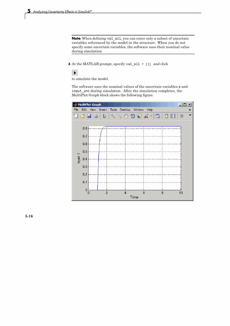
7/30/2019 Robust Control Toolbox User's Guide
http://slidepdf.com/reader/full/robust-control-toolbox-users-guide 162/180
MultiPlot Graph block shows the following figure.
5-16
Simulating Uncertainty Effects
4 Generate random samples of uncertainty values:
a Find all Uncertain State Space blocks and associated uncertain variables
in the model.
uvars=ufind('rct_sim_ex2')
MATLAB returns the following result:
uvars =
a: [1x1 ureal]
input_unc: [1x1 ultidyn]
The uncertain variables a and input_unc are ureal and ultidyn objects,
respectively and the structure uvars lists them by name

7/30/2019 Robust Control Toolbox User's Guide
http://slidepdf.com/reader/full/robust-control-toolbox-users-guide 163/180
respectively and the structure uvars lists them by name.
b Randomly sample the uncertain variables.
val_all = usample(uvars)
MATLAB returns the following result:
val_all =
a: -1.1167
input_unc: [1x1 ss]
The structure val_all contains sample values of the uncertain variables
a and input_unc. The software samples the values within the specified
uncertainty ranges for a and input_unc.
5 Simulate the model for the uncertainty values val_all. By repeating the
process inside a for-loop, you can assess how uncertainty affects the model
responses. For example, perform 10 simulations using random uncertainty
values:
for i=1:10;
val_all = usample(uvars)
sim('rct_sim_ex2',10);
end
5-17
5 Analyzing Uncertainty Effects in Simulink®
During each simulation, the software samples values of the uncertain
variables input_unc and a and plots the response for the sampled values. The
MultiPlot Graph block shows the following responses obtained using random
sample values of uncertain variables.
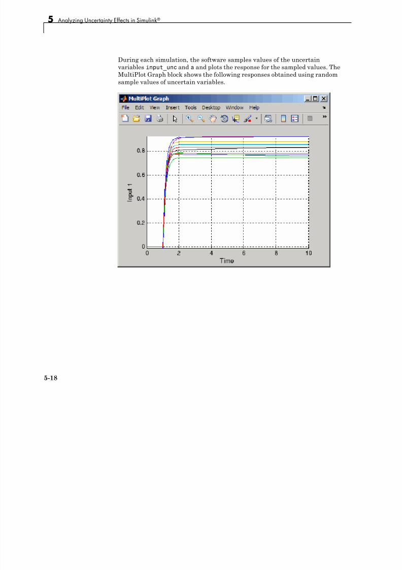
7/30/2019 Robust Control Toolbox User's Guide
http://slidepdf.com/reader/full/robust-control-toolbox-users-guide 164/180
5-18
Computing Uncertain State-Space Models from Simulink® Models
Computing Uncertain State-Space Models from Simulink Models
• “Ways to Compute Uncertain State-Space Models from Simulink Models”on page 5-19
• “Working with Models Containing Uncertain State Space Blocks” on page
5-19
• “Working with Models Containing Core Simulink or Custom Blocks” on
page 5-20
• “Next Steps” on page 5-25
Ways to Compute Uncertain State-Space Modelsf Si li k M d l
7/30/2019 Robust Control Toolbox User's Guide
http://slidepdf.com/reader/full/robust-control-toolbox-users-guide 165/180
from Simulink ModelsWhen you have the Simulink Control Design software, you can compute anuncertain linearization, i.e., an uncertain state-space model (uss) combining
the uncertain variables with linearized dynamics. Use the uss model to
perform linear analysis and robust control design.
You can compute an uncertain linearization in one of the following ways:
• Using the ulinearize command, as described in “Working with Models
Containing Uncertain State Space Blocks” on page 5-19.
• Using the Simulink Control Design linearize command, as described
in “Working with Models Containing Core Simulink or Custom Blocks”on page 5-20.
Working with Models Containing Uncertain StateSpace BlocksTo obtain an uncertain state-space model from a Simulink model that contains
Uncertain State Space blocks, use the following steps:
Note If you do not have Uncertain State Space blocks in the model but stillwant to obtain an uncertain state-space model, see “Working with Models
Containing Core Simulink or Custom Blocks” on page 5-20.
5-19
5 Analyzing Uncertainty Effects in Simulink®
1 (Prerequisite) Create or open the Simulink model.
2 (Prerequisite) In the Simulink model, specify the linearization input
and output points using Simulink Control Design getlinio or linio
commands. For more information, see “Selecting Inputs and Outputs for
the Linearized Model” in the Simulink Control Design documentation.
3 (Prerequisite) If you have not already done so, specify uncertainty in the
Simulink model as described in “Specifying Uncertainty Using Uncertain
State Space Blocks” on page 5-5.
Note The software does not evaluate the uncertain variables duringlinearization. Thus, the value of the uncertainty does not affect the
linearization.

7/30/2019 Robust Control Toolbox User's Guide
http://slidepdf.com/reader/full/robust-control-toolbox-users-guide 166/180
4 Run ulinearize to compute an uncertain linearization. This command
returns an uss model.
Note If you use the Simulink Control Designlinearize command, the
Uncertain State Space blocks linearize to their nominal value.
For more information on linearization and how to evaluate the results, see
“Linearization” in the Simulink Control Design documentation.
For an example of how to use the Simulink Control Design linearizecommand, see the Linearization of Simulink Models with Uncertainty demo.
Working with Models Containing Core Simulink orCustom BlocksIn some cases, you cannot use Uncertain State Space blocks in the Simulink
model because you share the model or generate code. You can still account
for uncertainty in your linear analysis without specifying uncertainty usingUncertain State Space blocks. Robust Control Toolbox lets you specify a
core or custom Simulink block to linearize to an uncertain variable. The
linearization produces an uncertain state-space uss model. The specified
5-20
Computing Uncertain State-Space Models from Simulink® Models
uncertainty associates only with the block and does not affect the model
simulation. For more information, see “Controlling Block Linearization” in
the Simulink Control Design User’s Guide.
Note If you have Uncertain State Space blocks in the model and want to
obtain an uncertain state-space model, see “Working with Models Containing
Uncertain State Space Blocks” on page 5-19.
To specify blocks to linearize to uncertain variables and obtain an uncertain
state-space model:
1 (Prerequisite) Create or open the Simulink model.
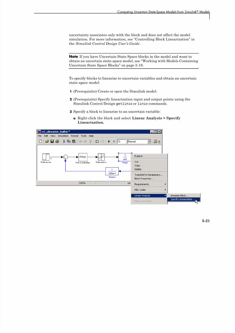
7/30/2019 Robust Control Toolbox User's Guide
http://slidepdf.com/reader/full/robust-control-toolbox-users-guide 167/180
2 (Prerequisite) Specify linearization input and output points using the
Simulink Control Design getlinio or linio commands.
3 Specify a block to linearize to an uncertain variable:
a Right-click the block and select Linear Analysis > Specify
Linearization.
5-21
5 Analyzing Uncertainty Effects in Simulink®
This action opens the Block Linearization Specification dialog box.
b In the Block Linearization Specification dialog box, select theSpecify
block linearization using a check box. Selecting this check box lets
you to specify an uncertain variable for linearization.

7/30/2019 Robust Control Toolbox User's Guide
http://slidepdf.com/reader/full/robust-control-toolbox-users-guide 168/180
This check box defaults to MATLAB Expression in the drop-down menu.
This option lets you specify the block to linearize to an uncertain
variable using a MATLAB expression containing Robust Control Toolbox
functions. To learn more about the options, see “Controlling Block
Linearization” in the Simulink Control Design documentation.
c In the Enter an expression to specify the linearization of the
Simulink block field, enter an expression, which must evaluate to an
uncertain variable or uncertain model, such as ureal, umat, ultidyn
or uss.
d Click OK to save the changes.
5-22
Computing Uncertain State-Space Models from Simulink® Models
Note You can also specify a block to linearize to an uncertain variable at
the command line. For an example, see “Example - Specifying a Block to
Linearize To an Uncertain Variable at the Command Line” on page 5-23.
4 Run the linearize command to compute an uncertain linearization. This
command returns an uss model.
For more information on linearization and how to validate linearization
results, see “Linearization” in the Simulink Control Design documentation.
For an example of how to use the linearize command to compute anuncertain linearization, see the Linearization of Simulink Models with
Uncertainty demo.

7/30/2019 Robust Control Toolbox User's Guide
http://slidepdf.com/reader/full/robust-control-toolbox-users-guide 169/180
Example - Specifying a Block to Linearize To an Uncertain Variable at the Command LineThis example demonstrates how to specify a core Simulink block to linearize to
an uncertain variable and compute an uncertain linearization at the commandline. To learn how to perform this task using the user interface, see “Working
with Models Containing Core Simulink or Custom Blocks” on page 5-20.
1 Open the Simulink model.
sldemo_f14
2 Double-click the Aircraft Dynamics Model block to view the subsystem.
5-23
5 Analyzing Uncertainty Effects in Simulink®

7/30/2019 Robust Control Toolbox User's Guide
http://slidepdf.com/reader/full/robust-control-toolbox-users-guide 170/180
3 Specify uncertain variables for the gain blocks Zd and Mw in the Aircraft
Dynamics Model subsystem.
spec.Type = 'Expression';
spec.Specification = ureal('Zd',-63.9979,'Percentage',20);
BlockSubs(1) = struct('Name','sldemo_f14/Aircraft Dynamics Model/Gain5','Value',spec);
spec.Specification = ureal('Mw',-63.9979,'Percentage',20);BlockSubs(2) = struct('Name','sldemo_f14/Aircraft Dynamics Model/Gain4','Value',spec);
4 Compute the uncertain linearization.
5-24
Computing Uncertain State-Space Models from Simulink® Models
mdl='sldemo_f14';
sys=linearize(mdl,BlockSubs)
MATLAB returns an uncertain state-space model, as shown in the followingresults:
USS: 7 States, 2 Outputs, 1 Input, Continuous System
Mw: real, nominal = -64, variability = [-20 20]%, 1 occurrence
Zd: real, nominal = -64, variability = [-20 20]%, 1 occurrence
Next Steps
After computing an uncertain linearization, you can perform one of thefollowing:
• Perform robustness analysis, as described in Chapter 2, “Generalized

7/30/2019 Robust Control Toolbox User's Guide
http://slidepdf.com/reader/full/robust-control-toolbox-users-guide 171/180
Robustness Analysis”.
• Perform robust control design, as described in “H-Infinity and Mu
Synthesis”.
5-25
5 Analyzing Uncertainty Effects in Simulink®
Analyzing Stability Margins
• “Using the loopmargin Command” on page 5-26
• “How Stability Margin Analysis Using Loopmargin Differs BetweenSimulink and LTI Models” on page 5-26
• “How to Analyze Stability Margin of Simulink Models” on page 5-27
• “Example — Computing Stability Margins of a Simulink Model” on page
5-28
Using the loopmargin CommandRobust Control Toolbox provides the loopmargin command to analyze the
stability margins of LTI models created in MATLAB and Simulink models.
To use loopmargin with Simulink models, you must have the Simulink
Control Design software This section describes the difference between the

7/30/2019 Robust Control Toolbox User's Guide
http://slidepdf.com/reader/full/robust-control-toolbox-users-guide 172/180
Control Design software. This section describes the difference between the
MATLAB and Simulink approaches of using loopmargin and the workflow for
computing the stability margin of Simulinkmodels. For more information on
how to analyze the stability margins of LTI models, see “Nominal Stability
Margins” section in the Robust Control Toolbox Getting Started Guide.
How Stability Margin Analysis Using LoopmarginDiffers Between Simulink and LTI ModelsWhen analyzing stability margins of LTI models using the syntax [cm,dm,mm]
= loopmargin(P,C), the software assumes the input and output of the linear
plant P as the margin analysis points, as shown in the following figure.
5-26
Analyzing Stability Margins
Analyzing stability margin of Simulink models differs from analyzing stability
margin of LTI models because you can enter specific margin analysis points in
the Simulink model For more information on ho to assign margin anal sis
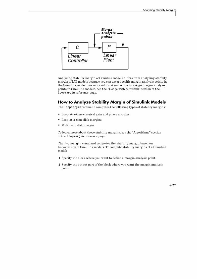
7/30/2019 Robust Control Toolbox User's Guide
http://slidepdf.com/reader/full/robust-control-toolbox-users-guide 173/180
the Simulink model. For more information on how to assign margin analysis
points in Simulink models, see the “Usage with Simulink” section of the
loopmargin reference page.
How to Analyze Stability Margin of Simulink ModelsThe loopmargin command computes the following types of stability margins:
• Loop-at-a-time classical gain and phase margins
• Loop-at-a-time disk margins
• Multi-loop disk margin
To learn more about these stability margins, see the “Algorithms” sectionof the loopmargin reference page.
The loopmargin command computes the stability margin based on
linearization of Simulink models. To compute stability margins of a Simulink
model:
1 Specify the block where you want to define a margin analysis point.
2 Specify the output port of the block where you want the margin analysis
point.
5-27
5 Analyzing Uncertainty Effects in Simulink®
The software performs the analysis by opening the loop at all specified
margin analysis point.
3 Use the loopmargin command to compute the stability margins at the
margin analysis point.
Optionally, you can compare the classical gain and phase margins obtained
using loopmargin with the stability margins computed for the linearized
model. The results using the two approaches should match for simple SISO
models. For MIMO models, the loopmargin command provides richer
robustness information. For an example, see “Example — Computing
Stability Margins of a Simulink Model” on page 5-28.
Additionally, you can compute stability margins by specifying multiple
margin analysis points and multiple operating points. For an example, see
the Loop Margins for an Airframe Autopilot demo.
7/30/2019 Robust Control Toolbox User's Guide
http://slidepdf.com/reader/full/robust-control-toolbox-users-guide 174/180
Example — Computing Stability Margins of aSimulink Model
This example illustrates how to compute the stability margins of theairframemargin model and compare the results with stability margins
computed using the linearized model.
1 Open the Simulink model:
airframemargin
The Simulink model, as shown in the following figure opens.
5-28
Analyzing Stability Margins

7/30/2019 Robust Control Toolbox User's Guide
http://slidepdf.com/reader/full/robust-control-toolbox-users-guide 175/180
2 Define a margin analysis point at the output of the Airframe Model block
by typing:
block1 = 'airframemargin/Airframe Model';
3 Specify the output az of the Airframe Model block as a margin analysis
point by typing:
port1 = 1;
4 Compute stability margins by typing:
[cm,dm,mm] = loopmargin('airframemargin',block1,port1);
5 View the classical gain and phase margins:
5-29
5 Analyzing Uncertainty Effects in Simulink®
cm
MATLAB return the following results:
cm =
GainMargin: [4.5652 2.5055e+003]
GMFrequency: [7.1979 314.1593]
PhaseMargin: 65.1907
PMFrequency: 2.1463
DelayMargin: 53.0113
DMFrequency: 2.1463
Stable: 1
6 Compare the classical gain and phase margins cm with stability margins of
the linearized model computed using allmargin:

7/30/2019 Robust Control Toolbox User's Guide
http://slidepdf.com/reader/full/robust-control-toolbox-users-guide 176/180
% Define linearization I/O points.
io = linio('airframemargin/Airframe Model',1,'outin','on');
% Linearize the model.
lin_sys = linearize('airframemargin',io);
% Compute gain and phase margins.
cm_lin = allmargin(-lin_sys);
MATLAB returns the following results:
cm_lin =
GainMargin: [4.5652 2.5055e+003]
GMFrequency: [7.1979 314.1593]PhaseMargin: 65.1907
PMFrequency: 2.1463
DelayMargin: 53.0113
DMFrequency: 2.1463
Stable: 1
The gain and phase margins, cm and cm_lin, computed using the two
approaches match.
5-30
A
Examples
Use this list to find examples in the documentation.

7/30/2019 Robust Control Toolbox User's Guide
http://slidepdf.com/reader/full/robust-control-toolbox-users-guide 177/180
A Examples
Building Uncertain Models“Generating One Sample” on page 1-45
“Generating Many Samples” on page 1-45
“Sampling ultidyn Atoms” on page 1-46
“Creating Arrays with stack and cat Functions” on page 1-53
“Creating Arrays by Assignment” on page 1-55
“Creating Arrays with usample” on page 1-57
“Creating Arrays with usubs” on page 1-58
“Creating Arrays with gridureal” on page 1-59
“Creating Arrays with repmat” on page 1-60

7/30/2019 Robust Control Toolbox User's Guide
http://slidepdf.com/reader/full/robust-control-toolbox-users-guide 178/180
A-2
The LMI Lab
The LMI Lab“Example: Specifying LMI Systems” on page 4-9
“Example: Minimizing Linear Objectives under LMI Constraints” on page
4-23“Example: Specifying Matrix Variable Structures” on page 4-33
“Example: Specifying Interdependent Matrix Variables” on page 4-34

7/30/2019 Robust Control Toolbox User's Guide
http://slidepdf.com/reader/full/robust-control-toolbox-users-guide 179/180
A-3
A Examples
Analyzing Uncertainty Effects in Simulink “Varying Uncertainty Values Using Individual Uncertain State Space
Blocks” on page 5-9
“Varying Uncertainty Values Across Multiple Uncertain State SpaceBlocks” on page 5-14
“Example - Specifying a Block to Linearize To an Uncertain Variable at
the Command Line” on page 5-23
“Example — Computing Stability Margins of a Simulink Model” on page
5-28

7/30/2019 Robust Control Toolbox User's Guide
http://slidepdf.com/reader/full/robust-control-toolbox-users-guide 180/180
A-4