Robust Centerline Extraction from Tubular Structures inMedical Images

Jianfei Liu Kalpathi Subramanian

Charlotte Visualization CenterDepartment of Computer Science

The University of North Carolina at CharlotteCharlotte, North Carolina, USA

ABSTRACT

Extraction of centerlines is useful to analyzing objects in medical images, such as lung, bronchia, blood vessels,and colon. Given the noise and other imaging artifacts that are present in medical images, it is crucial to userobust algorithms that are (1) noise tolerant, (2) computationally efficient, (3) accurate and (4) preferably, donot require an accurate segmentation and can directly operate on grayscale data. We propose a new centerlineextraction method that employs a Gaussian type probability model to build a more robust distance field. Themodel is computed using an integration of the image gradient field, in order to estimate boundaries of interest.Probabilities assigned to boundary voxels are then used to compute a modified distance field. Standard distancefield algorithms are then applied to extract the centerline. We illustrate the accuracy and robustness of ouralgorithm on a synthetically generated example volume and a radiologist supervised segmented head MRTangiography dataset with significant amounts of Gaussian noise, as well as on three publicly available medicalvolume datasets. Comparison to traditional distance field algorithms is also presented.

Keywords: virtual endoscopy, centerline, noise, medical imaging, skeleton, probability model

1. INTRODUCTION

The extraction of centerlines is useful to routine medical image analysis tasks, such as navigating the interiorsof colon, blood vessels, lungs and other tubular structures. Centerlines are a special case of medial surfaces (orskeletons) that have been studied extensively. Review articles on these and their related algorithms have recentlyappeared,1 that have precise definitions and requirements2 of these structures for a variety of applications thatspan navigation, image/volume registration, animation, morphing, recognition and retrieval.

Our focus in this work is toward robust centerline extraction from medical images and volumes, specificallywithin noisy environments. The approach we present does not require an accurate segmentation of the object;we estimate the boundary probabilistically using an integration of the image gradient field. The computedprobability field is then used to build a more robust distance field, after which we extract the object centerlineusing existing distance field based algorithms. We demonstrate the power and usefulness of our model by testingit on a set of synthetically generated volumes, as well as on publicly available medical imaging datasets. Theseexperiments were done using significant amounts of gaussian noise added to the datasets. Accuracy is quantifiedusing the synthetic model as well as the segmented medical dataset, and for comparison to traditional distancefield methods. We have successfully tested this approach on medical imaging datasets from blood vessel geometryin the brain, and a CT dataset of a human colon. We also have used interactive tools to qualitatively verify theaccuracy of our centerline in the medical datasets, in the absence of an accurate segmentation.

Further author information: (Send correspondence to Kalpathi Subramanian, krs@uncc.edu)Jianfei Liu: E-mail: jliu1@uncc.edu, Telephone: 1 704 687 8641Kalpathi Subramanian: E-mail: krs@uncc.edu, Web: www.cs.uncc.edu/∼krs; Telephone: 1 704 687 8579

We will begin with a look at centerline extraction methods that are directly relevant to the work presentedhere, specifically those based on distance fields and image characteristics, and briefly mention other methods.We will then develop our probability model and present preliminary results.

Distance Field Methods. These methods use a distance function, which is a signed function from eachdata point, and most often, referring to the distance-to-closest surface (or distance from boundary, DFB). Suchdistant maps have been used to accurately represent binary (or segmented) volumes to control aliasing artifacts,3

extract skeletons.4 In centerline extraction algorithms, an additional distance, distance-from-source, DFS, whichrepresents the distance from a source point has also been employed. Various distance metrics have been used inthese algorithms, such as 1-2-3 metric,5 3-4-5 chamfer metric,6 or 10-14-17.7 Exact voxel distances (1−

√2−

√3),

assuming unit cube voxels) have also been used.2

A number of researchers have used a combination of distance fields and Dijsktra’s algorithms (shortest path,minimum spanning tree) in order to extract the object centerline; the primary idea in these schemes is totransform the object voxels (identified in a preprocessing step) into a weighted graph, with the weights beingdefined by the inverse of the computed distance metric. Then Dijkstra’s algorithm is applied to find the shortestpath between specified end points. Chen et al.7 used this approach but modify the shortest path voxels tothe maximal DFB voxels orthogonal to the path, while Zhou5 chooses among voxel clusters with the same DFSdistance. Bitter et al.8,9 use a heuristic that combines the DFS and the DFB distances, with the latter beingconsidered a penalty aimed at discouraging the “hugging corner” problem, that is typical of shortest path basedapproaches. Finally, Wan et al.2 propose a method that also uses both DFS and DFB distances, but emphasizesthe latter to keep the centerline close to the center of the tubular structure. They also use a priority heap whichalways keeps the voxels close to the center at the top of the heap.

There are two strengths to distance field based methods, (1) outside of the distance field calculation, centerlineextraction algorithm is itself quite efficient, and, (2) the centerline is guaranteed to be inside the structure.However, all of these methods begin with a binary image, and for medical images, this means an accuratelysegmented image. This, in of itself, is a significant task, given that the original images can be considerably noisy(depending on their modality) and of poor contrast, and the presence of interfering organs can make this taskeven harder.

Image Characteristics. Methods in this category have been used in analyzing tubular structures in medicalimages, in particular, blood vessel geometry. They are based on two properties of images, (1) use of second orderderivatives, and (2) multi-scale analysis. Second order structure of an image is defined by the Hessian matrix,for instance, from a Taylor series expansion about a point x0,

I(x0 + δx0, σ) ≈ I(x0, σ) + δxT0 ∆0,σ + δxT

0 H0,σδx0 (1)

where ∆0,s and H0,s are the gradient and Hessian of the image at x0 at a scale s. Secondly, scale space theory10,11

relates scale to derivatives, which can be defined as convolution with derivatives of Gaussians:

∂

∂xI(x, s) = σγI(x) ∗ ∂

∂xG(x, σ) (2)

where G is a Gaussian with zero mean and deviation of σ. Parameter γ, introduced by Lindeberg12 helps definenormalized derivatives and provides the intuition for the use of scale in analyzing image structures.

In the work of Frangi et al.,13 the Hessian is used in detecting blood vessels from angiographic images. Eigenvectors of the Hessian matrix are used to determine the principal directions of the vessel structure; in particular,the direction with the smallest eigen (absolute) value points along the vessel axis, while the remaining two(orthogonal) direction vectors are along the vessel cross-section. This forms the basis for vessel detection, whichwhen combined with scale, can handle vessels of varying cross-section, given the results of Eq. 2, that relate scaleto boundary position.

Aylward14 formulated these ideas in proposing a centerline extraction method for blood vessel structures.Their approach was to identify and track ridges within angiographic images. Their method uses dynamic scale

enhancements to handle changes in vessel geometry, as well as perform well in the presence of noise. Wink etal.15 also use a multi-scale representation, however, they convert their multiscale “centeredness” measure toa cost (by choosing the largest response across a range of scales) and extract the centerline by computing theminimum cost path using Dijkstra’s algorithm. Potential to cope with severe stenoses was illustrated. Finally,ridge analysis in images has also been studied in detail by Eberly at al.,16,17 and tubular structure detection.18

Computing second order derivatives followed by eigen value analysis can be expensive, especially for verylarge medical objects. Nevertheless, secondary structure properties provide useful information for image analysisand we are looking into approaches to minimize computation and make these techniques more scalable.

Other Methods. A number of other methods have been proposed, including those based on field functions toextract skeletons. Examples of these include the use of potential functions19 and more recently, using topologicalcharacteristics derived from repulsive force fields.20 Radial basis functions21 have also been used. Some of thesemethods work in continuous space, which can potentially move the centerline out of the object, however, theyare more flexible, smoother and are less sensitive to noise due to averaging effects. Our proposed method alsotakes advantage of this property, as we integrate over a smooth gradient field of the image. Another class ofalgorithms is based on thinning;22 in general, these algorithms are quite expensive, but they are indeed quiterobust.

2. METHODS

2.1. Volume Preprocessing

The input volume is first roughly segmented into object voxels and background voxels. In our experiments, wehave used thresholding or region growing to isolate the object of interest. However, other more sophisticatedoperators might be necessary for complex datasets, several examples of which can be found in the Tuebingenarchive,23 and which we have also used to test our methodology.

2.2. Boundary Model

(a) (b) (c)x 0 00 −σ σ

Figure 1. (a) Step edge: ideal boundary, (b)Change in gradient magnitude (approximated by a Gaussian), (c) integralof gradient: blurred edge (also error function)

Medical images, by their nature of acquisition and reconstruction are bandlimited; thus, boundaries separatingmedical structures can be assumed to be blurred by a Gaussian. Fig. 1 (reproduced from24 illustrates a stepedge and its blurring by a Gaussian. While Kindlmann24 used this model to build transfer functions, our goalhere is to define a probability function across the object boundary. Specifically, we define the derivative of theimage intensity function f(x), or the gradient, as

f ′(x) =K√2πσ

e−x2

2σ2 (3)

where f ′(x) is centered around the point x, K is a normalizing constant and σ represents the deviation. Inte-grating Eq. 3 results in the familiar blurred boundary, as shown in Fig. 1c.

2.3. Normalizing the Boundary Probability Model

Our next step is to estimate the constant K, in order to determine the probability function for voxels close tothe boundary. We first evaluate Eq. 3 at x = 0 and x = ±σ,

f ′(0) =K√2πσ

(4)

f ′(σ) = f ′(−σ) =K√2πσ

e−12 (5)

Thus

f ′(σ)f ′(0)

=f ′(−σ)f ′(0)

= e−12 (6)

Consider Fig. 1b. f ′(0) occurs when the gradient magnitude attains a maximum, with (−σ, σ) on either side ofit. We use the following procedure to estimate K with respect to each boundary voxel:

1. Starting from each boundary voxel, determine the tracking direction (along the gradient direction, ~g or −~g)that leads to the local maximum; increasing gradient magnitude leads toward the boundary and decreasingmagnitude leads away from it.

2. Determine the local maxima of the gradient magnitude by moving along the gradient direction, ~g or −~g

3. Beginning from position x = 0, move along ~g or −~g to determine −σ and σ respectively. By using Eqn. 6,we can stop when the ratio reaches approximately e−1/2.

4. We know that ∫ 0

−∞f ′(x)dx =

∫ ∞

0

f ′(x)dx =K

2(7)

which is approximately ∫ 0

−σ

f ′(x)dx =∫ σ

0

f ′(x)dx =K

2(8)

as we are using K to make the area under the Gaussian equal to 1 (in order to convert it into a probabilitydensity function). The above equation thus gives us two possible estimates for K, denoted K1,K2. Due tothe fact that we are operating in a discrete lattice and the approximations involved in the boundary model,we cannot expect a perfectly symmetric Gaussian shaped variation of gradient across the object boundary.In other words, the points at which −σ and σ are calculated will usually be at differing distances fromx = 0. Choose K = MIN(K1,K2).

5. There are 5 possible cases:

• K1 < K2: This is illustrated in Fig. 2a. The shaded area (integral of the gradient) on the left issmaller, which is directly proportional to the estimate of K1

• K1 > K2: Similarly, as shown in Fig. 2b, the shaded area on the left is larger.

• K1 cannot be determined (Case 3) and K2 cannot be determined (Case 4): These two cases canhappen, if there are interfering structures that prevent calculating one of the estimates (detected bya sudden increase in gradient integral). In this case, we choose the computed estimate, K1 or K2.

• Neither K1 nor K2 can be estimated: This is rare, as in this case, the boundary is poorly defined andthe presegmentation has performed a poor job of obtaining the rough object boundary.

00

(a) (b)−σx1 = σx2=−σx1 = σx2=

−σx1 = σx2=(c) (d)

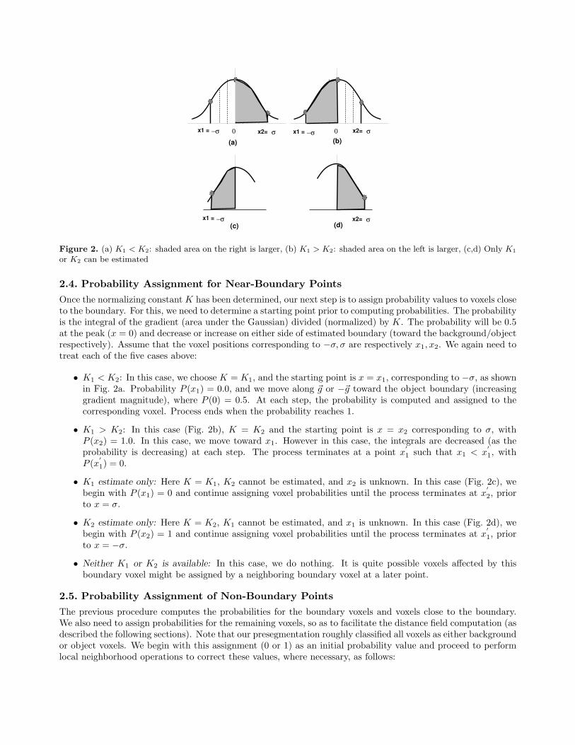
Figure 2. (a) K1 < K2: shaded area on the right is larger, (b) K1 > K2: shaded area on the left is larger, (c,d) Only K1

or K2 can be estimated

2.4. Probability Assignment for Near-Boundary Points

Once the normalizing constant K has been determined, our next step is to assign probability values to voxels closeto the boundary. For this, we need to determine a starting point prior to computing probabilities. The probabilityis the integral of the gradient (area under the Gaussian) divided (normalized) by K. The probability will be 0.5at the peak (x = 0) and decrease or increase on either side of estimated boundary (toward the background/objectrespectively). Assume that the voxel positions corresponding to −σ, σ are respectively x1, x2. We again need totreat each of the five cases above:

• K1 < K2: In this case, we choose K = K1, and the starting point is x = x1, corresponding to −σ, as shownin Fig. 2a. Probability P (x1) = 0.0, and we move along ~g or −~g toward the object boundary (increasinggradient magnitude), where P (0) = 0.5. At each step, the probability is computed and assigned to thecorresponding voxel. Process ends when the probability reaches 1.

• K1 > K2: In this case (Fig. 2b), K = K2 and the starting point is x = x2 corresponding to σ, withP (x2) = 1.0. In this case, we move toward x1. However in this case, the integrals are decreased (as theprobability is decreasing) at each step. The process terminates at a point x

′

1 such that x1 < x′

1, withP (x

′

1) = 0.

• K1 estimate only: Here K = K1, K2 cannot be estimated, and x2 is unknown. In this case (Fig. 2c), webegin with P (x1) = 0 and continue assigning voxel probabilities until the process terminates at x

′

2, priorto x = σ.

• K2 estimate only: Here K = K2, K1 cannot be estimated, and x1 is unknown. In this case (Fig. 2d), webegin with P (x2) = 1 and continue assigning voxel probabilities until the process terminates at x

′

1, priorto x = −σ.

• Neither K1 or K2 is available: In this case, we do nothing. It is quite possible voxels affected by thisboundary voxel might be assigned by a neighboring boundary voxel at a later point.

2.5. Probability Assignment of Non-Boundary Points

The previous procedure computes the probabilities for the boundary voxels and voxels close to the boundary.We also need to assign probabilities for the remaining voxels, so as to facilitate the distance field computation (asdescribed the following sections). Note that our presegmentation roughly classified all voxels as either backgroundor object voxels. We begin with this assignment (0 or 1) as an initial probability value and proceed to performlocal neighborhood operations to correct these values, where necessary, as follows:

A B

PB

PA

Figure 3. Modified distance field computation.

• For each unassigned voxel, vx on the object, compute the average probability, Pavg within its 26 connectedneighborhood. Pavg is thresholded against a background threshold Tbgrnd, and an object threshold, Tobj .

P (vx) ={

0, if Pavg < Tbgrnd

1, if Pavg > Tobj(9)

• If (Tbgrnd < Pavg < Tobj), the voxel’s probability is determined by looking at a fixed number of localneighbors (we use 2) along the gradient direction on either side of the voxel.

2.6. Distance Field ConstructionAs mentioned earlier, the principal goal of building the probability function is to have a more accurate descriptionof the boundary. We exploit this in building a distance field that is more accurate and of higher precision. Inparticular, the boundary voxels will have non-zero distances, in contrast to traditional distance fields where alldistances at the boundary start out with zero. Secondly, distance computation and propagation is also different.

Consider Fig. 3. PA and PB represent the probabilities assigned to points A and B. We compute the distancesDA and DB , from B and A respectively are calculated as follows:

DA = DB + PA D(B,A) (10)DB = DA + PB D(A,B) (11)

In other words, we scale the distance between the points, D(A,B), by the probability of the point being on theboundary. The traditional distance field algorithm assumes PA = PB = 1.

Using the above formulation, we compute the distance field using the approach of Gagvani.4 In our imple-mentation, we use exact voxel distances, 1−

√2−

√3 for isotropic volumes, or the actual voxel distances based

on the voxel size.

2.7. Centerline ExtractionOnce the distance field has been computed, we can now extract the centerline from the volume. We use a slightvariant of the algorithm proposed by Wan et al.2∗. Currently we use the voxel with the largest DFB (distancefrom boundary) as the root of the minimum spanning tree (MST) (as detailed in Wan et al.2) in the centerlineextraction algorithm. We also keep track of the largest geodesic distance from this starting point (or DFS),which is then used to lead toward the root point, via the chain of links built during the MST construction.

3. RESULTSIn order to evaluate the accuracy and robustness of our algorithm, we have tested our centerline extractionmethod on both synthetic as well as publicly available medical imaging datasets†. Accuracy was measuredquantitatively on two datasets whose exact centerline is known, (1) a synthetic dataset, and, (2) a radiologistsupervised segmentation of a a head MRT dataset (Fig. 4). This is followed by experiments on three medicalimaging datasets with added noise to illustrate the robustness of our method.

∗We had to slightly modify this algorithm as the flowchart seemed to have some missing conditions.†Color images will be available at http://www.cs.uncc.edu/∼krs/publ.html

3.1. Implementation

Our centerline extraction algorithm has been implemented in C++ on Linux workstations. We have used theInsight toolkit (ITK)25 for some of the image processing operations and noise generation, and the VisualizationToolkit(VTK)26 for displaying the results. All interaction is provided using the Fast and Light Toolkit (FLTK)27‡

3.2. Experiments: Accuracy Analysis

We have used a synthetically generated volume of a curved, sinusoidally shaped cylinder (100×100×102 voxels,Fig. 4), as well as a radiologist supervised segmented head MRT dataset (256 × 320 × 128 voxels, Fig. 4) toevaluate the accuracy of our probabilistic centerline extraction method, and compare it with the traditionaldistance transform method. Our parameters of synthetically generated volume are similar to those used inAylward;14 background intensity level is set to 100 and the object voxels range from 150 at the boundary to200 at the center of the object. Because Gaussian noise is the most common in medical images, we added it(using ITK) to both datasets, with σ = 40 for the sinusoidal cylinder dataset, and σ = 20 for the head MRTdata. As described in Aylward,14 σ = 40 and above represents a worst case scenario, even for medical images.We computed the gradient magnitude field (using itk::GradientMagnitudeRecursiveGaussianImageFilter) withσ = 10 for the cylinder dataset and σ = 0.5 for MRT dataset.

Three accuracy measures similar to Aylward,14 were computed from the extracted centerline, as follows:

• Average Error: This represents the mean distance between corresponding points from the ideal centerlineand extracted centerline. Results can be ambiguous, depending on how the corresponding points arecomputed; in our implementation, we pick the larger of the two distances computed, starting from each ofthe two centerlines.

• Maximum Error: This represents the maximum distance between two corresponding points.

• Percent Points Within 1 Voxel: This represents the percentage of voxels on the extracted centerline thatare within 1 voxel of their closest ideal centerline point.

For the cylinder dataset, we know the exact location of the centerline, which enables us to measure theaccuracy of our algorithm under various conditions. For the segmented MRT head dataset, we first use thetraditional distance transform to extract the centerline from the segmented medical data by specifying startand end points on a a part of the relatively thick trunk. This result is considered as the ideal centerline inour experiments (our implementation closely follows,2 which is based on locating centerline voxels with thelargest distance from the boundary). Then we tested our algorithm on noisy MRT data. The volume was firstroughly segmented using thresholding. Both methods were then used on this dataset with the same start andend points(as used to compute the ideal centerline)

Fig. 4 illustrates the results on this dataset with added Gaussian noise with noise deviation, σ = 40 forthe cylinder dataset and σ = 20 for the MRT head dataset. The left column of images are generated usingour probabilistic distance transform method, while the images in the right column are generated using thetraditional distance transform method. The ideal centerline (in red) is overlaid with extracted centerline (inyellow). Significant errors can be noticed in the images in the right column. For spatial perspective, we alsooutput the isosurface (via the Marching Cubes algorithm28) of the object. At the higher noise levels, the isosurfaceadds more and more geometry, making it difficult to perceive the centerline. Hence we have made the isosurfacealmost fully transparent.

Table 1 displays the computed accuracy measures the for sinusoidal cylinder dataset and MRT head datasetboth with gaussian noise, σ = 20. Average errors of our method are between 0.7-1.3 voxels, vs. 3.0-5.7 voxelsusing the traditional distance form method. Maximum errors are also much smaller, 1.6-3.0 vs. 5.2-11.2 voxels,and over 73-97% of voxels are within 1 voxel, vs. 9-75% for the traditional method.

‡ITK, VTK and FLTK are open source toolkits that run across a number of different platforms

Figure 4. Comparison between traditional distance transform vs. probabilistic distance transform approach on sinusoidcylinder dataset (top row) at Noise level, σ = 40 and segmented head MRT (bottom row) data at Noise level, σ = 20.Ideal centerline(in red) overlaid on top of extracted centerline(in yellow). Left column: Using our probabilistic distancetransform method, Right column: Using traditional distance transform method.

Table 1. Centerline accuracy of sinusoid cylinder dataset at noise level 40 and head MRT data at noise level 20.

MeasuresData Trad. Dist. Transform/Prob. Dist. TransformType Avg. Error Max. Error % Pts Within 1 Voxel

Sinusoid Cyl. 5.7/1.3 11.2/3.0 9.1/73.5Head MRT 3.0/0.7 5.2/1.6 75.6/97.4

Figure 5. Aneurysm Dataset with no added noise (left) and noise level σ = 50.

Figure 6. Aneurysm Dataset.(Left:) No added noise, (Right:) Gaussian noise, σ = 20.

3.3. Experiments: Medical Data

Additionally, we have tested our algorithm with two medical volume datasets available from the archive atUniversity of Tuebingen,23 and a colon dataset available from the National Library of Medicine.29 We describeour experiments with these datasets next, in the presence of Gaussian noise.

Fig. 5 displays the results of the aneurysm dataset with no added noise (left), Gaussian (right) at a noiselevel, σ = 50. Centerlines were extracted on all vessels connected to the main trunk. As this vascular tree hasalso a significant number of disconnected structures as well as many extremely small vessels, it is a particularchallenging dataset. Here we show the isosurface of the vessels (for spatial perspective) from the clean (no noise)data, as otherwise the centerline is barely visible. Since it’s very hard to judge the results from thin branches,we focus on the resulting centerlines of the trunk. At high noise levels, there are a few spurious branches usingour method.

Fig. 6 shows the results of a second head MRT data with Gaussian noise at σ = 20. The isosurface isextracted from segmented data. The MRT data set has considerably weaker boundaries. As the vessels are justa few voxels wide, for noise levels of σ = 40 (not shown) and above, the centerline starts to exhibit errors. Thiscan also happen when small blood vessels are extremely close to each other, as encountered by Frangi.13 Thus,we also qualitatively verify the centeredness of our algorithm using 2D texture mapped planes (not shown),corresponding to axial, sagittal and coronal orientations.

Finally, we have tested our method on a colon dataset from the large archive at the National Library ofMedicine.29 Fig. 7 illustrates the effects of adding noise. The left image illustrates the dataset with no addednoise, and the right image with Gaussian noise added, at a noise level of σ = 20. In these images, the centerlineof the noisy dataset (in yellow) is overlaid on the centerline of the clean dataset (in red). Mid sections of the

Figure 7. Results:Analysis of colon dataset with added noise, σ = 20. Left: Centerline of colon dataset with no addednoise, Right: With gaussian noise, centerlines (in yellow) extracted from noisy dataset overlaid on clean dataset(in red).

Table 2. Running Times(secs): Medical Datasets

Resolution Running Times (seconds)Dataset (voxels) Prob. Model Constr./Centerline Extr.

σ = 0 σ = 20 σ = 25Aneurysm 256× 256× 256 114.1/8.0 114.3/8.1 114.3/8.1MRT 256× 320× 128 70.8/4.5 74.1/13.9 74.1/13.9Colon 409× 409× 220 424.7/40.9

section show very little error. The centerlines deviate at the beginning and the ending regions of the colon; thisis due to the differing start and end points used in the respective datasets.

Table 2 illustrates the running times for the three medical dataset examples with Gaussian noise. Probabilityfunction construction times range from 1-7 minutes. Similar to the synthetic datasets, running times can befurther improved by more properly handling volume boundary effects.

Figure 8. Comparison of using traditional distance fields vs. using probabilistically defined distance fields in centerlineextraction. Top three images show an axis-aligned cylinder with its centerline extracted using the algorithm by Wan etal.2 at noise levels of sigma = 0, 10, 20; bottom figure illustrates the object with a probabilistic boundary, with σ = 20.

4. DISCUSSION

The primary goal of this work was to extract centerlines of tubular structures in a robust and accurate fashion,without assumptions of exact boundaries. Complex datasets such as those used in this work and archived at23

are considerably challenging to traditional distance field algorithms, which assume a binary (usually thresholded)dataset and hence zero distance values on the boundary. Our main idea in this work is to determine a probabilisticestimate of the boundary location (in the spirit of24 for computing smooth transfer functions) and use theseto modify the traditional distance from boundary. We still take advantage of the speed of distance field basedalgorithms for centerline extraction.

An example of comparing our method to traditional distance field based centerline extraction is shown inFig. 8 for a simple example of an axis-aligned cylinder. The top three images illustrate the cylinder with noiselevels of σ = 0, 10 and 20. We use the method of Wan et al.2 We see the dramatic deviation of the centerlinefrom the horizontal as the noise level is increased. The bottom image illustrates our algorithm at σ = 20. Asillustrated in Table 1 the errors for the cylinder are very low even at very high noise levels.

We note with interest the use of the Hessian based methods coupled with multi-scale analysis13,14 to exploreand analyze highly complex medical datasets. These are generally computationally more expensive (as our initialinvestigations have revealed); this is especially the case if they have to be computed for all object voxels. We arecurrently looking into using the Hessian in a limited fashion, thus making it possible to use eigen value analysisfor larger medical structures.

5. CONCLUSIONS

We have presented a robust and accurate centerline extraction algorithm that can work with gray scale imagesand a rough segmentation of the structures of interest. The goal of this work is toward analyzing large medicalstructures of interest. We have presented a probabilistic model to estimate the boundary using an integration ofthe gradient field. The computed voxel probabilities were then used to build a modified distance field which isthen used to extract the centerline of the object. Preliminary experiments on both synthetic and clinical datasetsare promising. Accuracy within a voxel has been illustrated using this model. We have also tested our algorithmon three medical imaging datasets, including an aneurysm dataset, head MRT blood vessel dataset, and a colondataset. Comparisons to traditional distance field algorithms for centerline extraction illustrate the robustnessof this method within noisy environments.

The work presented here has focused on a centerline extraction algorithm that can work well in the presenceof noise. Several aspects of of this algorithm are incomplete, such as incorporating scale as part of this methodto adapt to more significant changes in object geometry. We are currently investigating these issues.

REFERENCES1. N. Cornea, D. Silver, and P. Min, “Curve-skeleton applications,” in Proceedings of IEEE Visualization 2005,

pp. 95–102, 2005.2. M. Wan, Z. Liang, I. Bitter, and A. Kaufman, “Automatic centerline extraction for virtual colonoscopy,”

IEEE Transactions on Medical Imaging 21(12), pp. 1450–1460, 2002.3. S. Gibson, “Using distance maps for accurate representation in sampled volumes,” in Proceedings of the

1998 IEEE Symposium on Volume Visualization, pp. 23–30, 1998.4. N. Gagvani and D. Gagvani, “Parameter controlled skeletonization of three dimensional objects,” Tech.

Rep. CAIP-TR-216, Rutgers University, 1997.5. Y. Zhou and A. Toga, “Efficient skeletonization of volumetric objects,” IEEE Transactions on Visualization

and Computer Graphics 5(3), pp. 196–209, 1999.6. G. Borgefors, “Distance transformations in digital images,” Computer Vision and Image Understanding 34,

pp. 344–371, 1986.7. D. Chen, B.Li, Z. Liang, M. Wan, A. Kaufman, and M. Wax, “A tree-branch searching multiresolution

approach to skeleteonization for virtual endoscopy,” in Proceedings of SPIE Medical Imaging, 3979, pp. 726–734, 2000.

8. I. Bitter, M. Sato, , M. Bender, K.McDonnel, A. Kaufman, and M. Wan, “Ceaser: A smooth, accurate androbust centerline-extraction algorithm,” in Proceedings of IEEE Visualization 2000, pp. 45–52, 2005.

9. I. Bitter, A. Kaufman, and M. Sato, “Penalized-distance volumetri skeleton algorithm,” IEEE Transactionson Visualization and Computer Graphics 7(3), pp. 195–206, 2002.

10. J. Koenderink, “The structure of images,” Biological Cybernetics 50, pp. 363–370, 1984.11. L. Florack, B. ter Haar Romeny, J. Koenderink, and M. Viergever, “Scale and the differential structure of

images,” Image and Vision Computing 10(6), pp. 376–388, 1992.12. T. Lindberg, “Feature detection with automatic scale selection,” Intrernational Journal of Computer Vi-

sion 30(2), pp. 79–116, 1998.13. A. Frangi, W. Niessen, K. Vincken, and M. Viergever, “Multiscale vessel enhancement filtering,” Lecture

Notes in Computer Science 1496, pp. 130–137, 1998. citeseer.ist.psu.edu/frangi98multiscale.html.14. S. Aylward and E. Bullitt, “Initialization, noise, singularities, and scale in height ridge traversal for tubular

object centerline extraction,” IEEE Transactions on Medical Imaging 21(2), pp. 61–75, 2002.15. O. Wink, W. Niessen, and M. Viergever, “Multiscale vessel tracking,” IEEE Transactions on Medical Imag-

ing 23(1), pp. 130–133, 2004.16. D. Eberly, R. Gardiner, B. Morse, S. Pizer, and C. Scharlach, “Ridges for image analysis,” Journal of

Mathematical Imaging and Vision 4, pp. 351–371, 1994.17. D. Eberly, Ridges in Image and Data Analysis (Computational Imaging and Vision), Springer, 1996.18. K. Krissian, G. Malandain, N. Ayache, R. Vaillant, and Y. Trousset, “Model based detection of tubular

structures in 3d images,” Tech. Rep. 3736, INRIA, Sophia Antipolis, France, 1999.19. J. Chuang, C. Tsai, and M. Kuo, “Skeletonization of three-dimensional object using generalized potential

field,” IEEE Transactions on Pattern Analysis and Machine Intelligence 22(11), pp. 1241–1251, 2000.20. N. Cornea, D. Silver, X. Yuan, and R. Balasubramanian, “Computing hierarchical curve-skeletons of 3d

objects,” Visual Computer 21(11), pp. 945–955, 2005.21. W.-C. Ma, F.-C. Wu, and M. Ouhyoung, “Skeleton extraction of 3d objects with radial basis functions,”

2003.22. C. M. Ma and M. Sonka, “A fully parallel 3d thinning algorithm and its applications,” Computer Vision

and Image Understanding 64(3), pp. 420–433, 1996.23. D. Bartz. http://www.gris.uni-tuebingen.de/areas/scivis/volren/datasets/new.html.24. G. Kindlmann and J. Durkin, “Semi-automatic generation of transfer functions for direct volume rendering,”

in Proceedings of the 1998 IEEE Symposium on Volume Visualization, pp. 79–86, 1998.25. T. Yoo, Insight into Images: Principles and Practice for Segmentation, Registration, and Image Analysis,

A.K. Peters, 2004. http://www.itk.org.26. W. Schroeder, K. Martin, and B. Lorensen, The Visualization Toolkit: An Object-Oriented Approach to 3D

Graphics, Prentice Hall Inc., 2002 (3th edition).27. B. Spitzak, “The fast light toolkit.” http://www.fltk.org.28. W. Lorensen and H. Cline, “Marching cubes: A high resolution 3d surface reconstruction algorithm,”

Computer Graphics 21(4), 1987.29. M. R. Choi. http://nova.nlm.nih.gov.