Robotics IIJanuary 11, 2018

Exercise 1

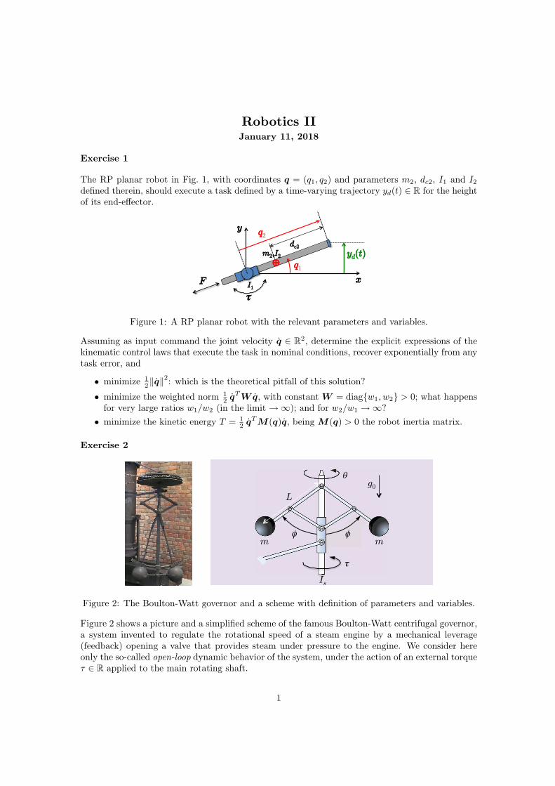
The RP planar robot in Fig. 1, with coordinates q = (q1, q2) and parameters m2, dc2, I1 and I2defined therein, should execute a task defined by a time-varying trajectory yd(t) ∈ R for the heightof its end-effector.

x I1

y

! q1

q2

m2,I2

dc2

!"

F

yd(t)

Figure 1: A RP planar robot with the relevant parameters and variables.

Assuming as input command the joint velocity q ∈ R2, determine the explicit expressions of thekinematic control laws that execute the task in nominal conditions, recover exponentially from anytask error, and

• minimize 12‖q‖

2: which is the theoretical pitfall of this solution?

• minimize the weighted norm 12 q

TWq, with constant W = diagw1, w2 > 0; what happensfor very large ratios w1/w2 (in the limit →∞); and for w2/w1 →∞?

• minimize the kinetic energy T = 12 q

TM(q)q, being M(q) > 0 the robot inertia matrix.

Exercise 2

OCTOBER 2016 « IEEE CONTROL SYSTEMS MAGAZINE 83

be positive. All coefficients in (11) are actually positive since they are physical quantities, and thus the system is stable if the third row value of the Routh array is positive, which gives the condition (12). However, since there was no Routh or Hurwitz stability criterion at that time, the next section of this article presents an alternative derivation of Maxwell’s stability criterion.

Next, Maxwell considered the dynamic equations of motion for the governors of Sir William Thomson and Léon Foucault. For the centrifugal pieces of Foucault’s governor,

shown in Figure 11, Maxwell expressed the equations of motion using the angular momentum Aio ,

,dtd A Li =o^ h (13)

!"#$#% i %&'%("#%)*+,#%-.%$#/-,0(&-*%)1-0(%("#%/#$(&2),%)3&'4%A%&'%("#%5-5#*(%-.%&*#$(&)%-.%)%$#/-,/&*+%)66)$)(0'%.-$% i %5-(&-*4%)*7%L %&'%("#%(-(),%(-$80#%)2(&*+%-*%("#%)3&'9%:#(%B%1#%("#%5-5#*(%-.%&*#$(&)%-.%("#%.,;1),,'%&*%Figure 11%.-$%z %5-(&-*9%<"#*4%("#%'05%-.%("#%=&*#(&2%)*7%6-(#*(&),%#*#$+&#'%-.%>-02)0,(?'%+-/#$*-$%&'

,E A B P Ld21

212 2i z i= + + =o o # (14)

where P is the potential energy of the apparatus, which is a function of the divergence angle z of the centrifugal piece. Here, A and B are both functions of the angle z . Differen-tiating (14) with respect to time t and using (13) gives

,A B P A B L A A21

212 2i z z ii zz i zi i i+ + + + = = +z z z zo o o o p o p o o o p oc ^m h

(15)

where the subscript z indicates ( )/d d: z . If the apparatus is arranged such that .P AV0 5 constant2= + , where V is a

!

"

FIGURE 11 The centrifugal pieces (that is, flyballs) of Foucault’s governor. A is the moment of inertia of a revolving apparatus for i motion, and B is the moment of inertia of flyballs for z motion.

PR

G!

"Y!

+ W

M B

m

r

k

r1

F ("–V1)

F ("–V1)

!

(a) (b)

FIGURE 10 A free-body diagram of Jenkin’s governor. The friction torque ( )F V1i -o acting on the friction ring is obtained by lineariza-tion about a constant speed V1 .

FIGURE 9 Siemens’ liquid governor. The speed of a drive shaft S is controlled according to the depth of immersion of a rotating cup C connected to the shaft by a screw and a spring E. For over-speed, the rotation of the cup C falls behind that of the shaft S. Forced downward by the thread, the cup C is immersed deeper into the liquid, thus pumping at a higher rate and exerting an in-creasing resistance torque on the drive shaft. [Reproduced with permission of W. Bowyer and J. Nichols for Lockyer Davis, printer to the Royal Society from [12] (CCC Licensed 3811700428077 and 3834140751528).]

!"

#"m m

Is

L

g0

#"

Figure 2: The Boulton-Watt governor and a scheme with definition of parameters and variables.

Figure 2 shows a picture and a simplified scheme of the famous Boulton-Watt centrifugal governor,a system invented to regulate the rotational speed of a steam engine by a mechanical leverage(feedback) opening a valve that provides steam under pressure to the engine. We consider hereonly the so-called open-loop dynamic behavior of the system, under the action of an external torqueτ ∈ R applied to the main rotating shaft.

1

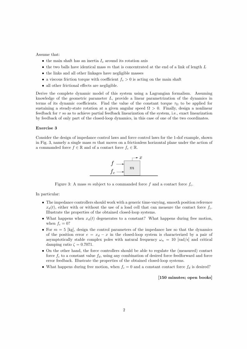
Assume that:• the main shaft has an inertia Is around its rotation axis• the two balls have identical mass m that is concentrated at the end of a link of length L

• the links and all other linkages have negligible masses• a viscous friction torque with coefficient fv > 0 is acting on the main shaft• all other frictional effects are negligible.

Derive the complete dynamic model of this system using a Lagrangian formalism. Assumingknowledge of the geometric parameter L, provide a linear parametrization of the dynamics interms of its dynamic coefficients. Find the value of the constant torque τΩ to be applied forsustaining a steady-state rotation at a given angular speed Ω > 0. Finally, design a nonlinearfeedback for τ so as to achieve partial feedback linearization of the system, i.e., exact linearizationby feedback of only part of the closed-loop dynamics, in this case of one of the two coordinates.

Exercise 3

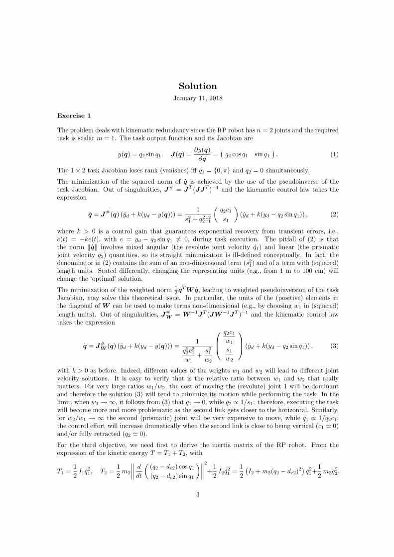
Consider the design of impedance control laws and force control laws for the 1-dof example, shownin Fig. 3, namely a single mass m that moves on a frictionless horizontal plane under the action ofa commanded force f ∈ R and of a contact force fc ∈ R.

Figure 3: A mass m subject to a commanded force f and a contact force fc.

In particular:

• The impedance controllers should work with a generic time-varying, smooth position referencexd(t), either with or without the use of a load cell that can measure the contact force fc.Illustrate the properties of the obtained closed-loop systems.

• What happens when xd(t) degenerates to a constant? What happens during free motion,when fc = 0?

• For m = 5 [kg], design the control parameters of the impedance law so that the dynamicsof the position error e = xd − x in the closed-loop system is characterized by a pair ofasymptotically stable complex poles with natural frequency ωn = 10 [rad/s] and criticaldamping ratio ζ = 0.7071.

• On the other hand, the force controllers should be able to regulate the (measured) contactforce fc to a constant value fd, using any combination of desired force feedforward and forceerror feedback. Illustrate the properties of the obtained closed-loop systems.

• What happens during free motion, when fc = 0 and a constant contact force fd is desired?

[150 minutes; open books]

2

SolutionJanuary 11, 2018

Exercise 1

The problem deals with kinematic redundancy since the RP robot has n = 2 joints and the requiredtask is scalar m = 1. The task output function and its Jacobian are

y(q) = q2 sin q1, J(q) =∂y(q)∂q

=(q2 cos q1 sin q1

). (1)

The 1× 2 task Jacobian loses rank (vanishes) iff q1 = 0, π and q2 = 0 simultaneously.

The minimization of the squared norm of q is achieved by the use of the pseudoinverse of thetask Jacobian. Out of singularities, J# = JT (JJT )−1 and the kinematic control law takes theexpression

q = J#(q) (yd + k(yd − y(q))) =1

s21 + q2

2c21

(q2c1

s1

)(yd + k(yd − q2 sin q1)) , (2)

where k > 0 is a control gain that guarantees exponential recovery from transient errors, i.e.,e(t) = −ke(t), with e = yd − q2 sin q1 6= 0, during task execution. The pitfall of (2) is thatthe norm ‖q‖ involves mixed angular (the revolute joint velocity q1) and linear (the prismaticjoint velocity q2) quantities, so its straight minimization is ill-defined conceptually. In fact, thedenominator in (2) contains the sum of an non-dimensional term (s2

1) and of a term with (squared)length units. Stated differently, changing the representing units (e.g., from 1 m to 100 cm) willchange the ‘optimal’ solution.

The minimization of the weighted norm 12 q

TWq, leading to weighted pseudoinversion of the taskJacobian, may solve this theoretical issue. In particular, the units of the (positive) elements inthe diagonal of W can be used to make terms non-dimensional (e.g., by choosing w1 in (squared)length units). Out of singularities, J#

W = W−1JT (JW−1JT )−1 and the kinematic control lawtakes the expression

q = J#W (q) (yd + k(yd − y(q))) =

1q22c

21

w1+s2

1

w2

q2c1w1

s1

w2

(yd + k(yd − q2 sin q1)) , (3)

with k > 0 as before. Indeed, different values of the weights w1 and w2 will lead to different jointvelocity solutions. It is easy to verify that is the relative ratio between w1 and w2 that reallymatters. For very large ratios w1/w2, the cost of moving the (revolute) joint 1 will be dominantand therefore the solution (3) will tend to minimize its motion while performing the task. In thelimit, when w1 →∞, it follows from (3) that q1 → 0, while q2 ∝ 1/s1: therefore, executing the taskwill become more and more problematic as the second link gets closer to the horizontal. Similarly,for w2/w1 → ∞ the second (prismatic) joint will be very expensive to move, while q1 ∝ 1/q2c1:the control effort will increase dramatically when the second link is close to being vertical (c1 ' 0)and/or fully retracted (q2 ' 0).

For the third objective, we need first to derive the inertia matrix of the RP robot. From theexpression of the kinetic energy T = T1 + T2, with

T1 =12I1q

21 , T2 =

12m2

∥∥∥∥ d

dt

((q2 − dc2) cos q1

(q2 − dc2) sin q1

)∥∥∥∥2

+12I2q

21 =

12(I2 +m2(q2 − dc2)2

)q21+

12m2q

22 ,

3

we obtain a diagonal inertia matrix as

M(q) =(I1 + I2 +m2(q2 − dc2)2 0

0 m2

)=(m11(q2) 0

0 m22

). (4)

The minimization of the kinetic energy T is then a special case of a weighted pseudoinversion ofthe task Jacobian, with one weight being configuration dependent. Thus, out of singularities, theinertia-weighted kinematic control law takes the expression

q = J#M (q) (yd + k(yd − y(q))) =

1q22c

21

m11(q2)+

s21

m22

q2c1

m11(q2)s1

m22

(yd + k(yd − q2 sin q1)) . (5)

Note that the two addends in the first denominator have both consistent units of [kg−1].

Exercise 2

Let q = (θ, φ). Following a Lagrangian approach, under the given assumptions, we compute thekinetic energy T = Ts + 2Tm for the main shaft and the two equal balls. We have

Ts =12Is θ

2, Tm =12mL2

(φ2 + θ2 sin2φ

),

and thus the diagonal inertia matrix

M(q) =(Is + 2mL2 sin2φ 0

0 2mL2

). (6)

Using the Christoffel symbols, the Coriolis and centrifugal terms are easily computed from (6) as

c(q, q) =

(4mL2 sinφ cosφ θ φ−2mL2 sinφ cosφ θ2

)= mL2 sin(2φ)

(2 θ φ− θ2

)(7)

For the potential energy due to gravity, U = Us + 2Um, we have (up to a constant)

Us = 0, Um = −mg0L cosφ,

and thus

g(q) =(∂U(q)∂q

)T=(

02mg0L sinφ

). (8)

Including also viscous friction on the main shaft, the dynamic equations are(Is + 2mL2 sin2φ

)θ + 4mL2 sinφ cosφ θ φ+ fv θ = τ

2mL2 φ− 2mL2 sinφ cosφ θ2 + 2mg0L sinφ = 0.(9)

Assuming knowledge of the geometric parameter L, equation (9) can be expressed in the linearlyparametrized form(

θ 2L2 sin2φ θ + 2L2 sin(2φ) θ φ θ

0 2L2 φ− L2 sin(2φ) θ2 + 2g0L sinφ 0

) Is

m

fv

= Y (q, q, q)π =(τ

0

), (10)

4

with the vector π ∈ R3 of dynamic coefficients.

In a steady-state equilibrium with constant angular velocity θ = Ω > 0, we have θ = 0 andφ = φ = 0. This yields from (9)

τΩ = fvΩ, L sinφ cosφ Ω2 + g0 sinφ = 0 ⇒ cosφe =g0

LΩ2. (11)

The input torque τΩ has to compensate just for the energy loss due to friction, in order to keep auniform motion via constant angular velocity. Moreover, the equilibrium angle φe results from thebalance of the gravity force and the centrifugal force. Its value increases (in the range (0, π/2))together with Ω.

Finally, by applying the nonlinear feedback law

τ =(Is + 2mL2 sin2φ

)a+ 4mL2 sinφ cosφ θ φ+ fv θ (12)

where a ∈ R is the new control input (an acceleration), system (9) is transformed into

θ = a

φ− sinφ cosφ θ2 +g0

Lsinφ = 0.

(13)

The dynamics of θ is now exactly linear (a double integrator), while partial control of the motion ofφ can be achieved only through the centrifugal term in the second equation, being θ2 =

(∫a dt)2.

Exercise 3

The dynamic equation of the system in Fig. 3 is

mx = f + fc. (14)

Impedance control. The so-called inverse dynamics control law becomes in this simple case

f = ma− fc, (15)

and transforms system (14) into the double integrator

x = a. (16)

The auxiliary input a has to be designed so that the controlled mass m, under the action of thecontact force fc, matches the behavior of an impedance model characterized by a desired (apparent)mass md > 0, desired damping kd > 0, and desired stiffness kp > 0, all acting with respect to asmooth motion reference xd(t), or

md (x− xd) + kd (x− xd) + kp (x− xd) = fc. (17)

Equating x in (16) and in the reference behavior (17), solving for a and substituting in (15) yieldsthe control force

f =m

md(xd + kd (xd − x) + kp (xd − x)) +

(m

md− 1)fc. (18)

The feedback law (18) requires in general a measure of the contact force fc.

5

In the reference model (17), the position error e = xd − x does not converge to zero if there isa contact force fc. Otherwise, e will asymptotically go to zero —indeed exponentially, in view ofthe linearity of the system dynamics. In particular, for k2

d < 4kpmd, the obtained second-orderlinear system (17) is characterized by a pair of asymptotically stable complex poles with naturalfrequency and damping ratio given by

ωn =√kpmd

, ζ =kd

2√kpmd

. (19)

Reducing the desired mass md, for given values of stiffness and damping, will increase both thenatural frequency ωn and the damping ratio ζ, and thus improve transients. On the other hand,for a given mass md, an increase of the stiffness kp should be accompanied by an increase ofthe damping kd in order to prevent more oscillatory transients. If the desired mass equals thenatural (original) mass, i.e., md = m, a measure of the contact force fc is no longer needed in theimpedance controller (18).

Wishing to achieve ωn = 10 and ζ = 0.7071 = 1/√

2, equations (19) provide

kp = 100md, kd = 10√

2md, for any md > 0. (20)

Being m = 5 [kg], if we take in particular md = m = 5, we obtain as gains

kp = 500, kd = 50√

2 = 70.71, (21)

and a measure of fc will not be needed.

In regulation tasks (with xd(t) = xd = constant), by choosing again md = m, the control law 18)collapses to just a PD action on the position error e,

f = kp (xd − x)− kdx. (22)

This scheme is also called compliance control, since the main design parameter left is the desiredstiffness kp. Also in this case, the system will converge to x = xd if (and only if) there is no contactforce. With fc 6= 0 but constant, the position xe 6= xd that satisfies

kp(xd − xe) + fc = 0 ⇒ xe = xd +fckp

(23)

will be an asyptotically (exponentially) stable closed-loop equilibrium, as can be possibly checkedwith the Lyapunov candidate V = 1

2mx2 + 1

2kp(x − xe)2 ≥ 0 (using in this case LaSalle theorem

for the analysis).

Force control. If we desire to regulate explicitly the contact force to a desired constant value fd,it is necessary to build a force error ef = fd − fc into the control law. After using (15), define theauxiliary input a as

a =1md

(kf (fd − fc)− kdx) , (24)

with force error gain kf > 0 and velocity damping coefficient kd > 0. The associated control forceis then

f =m

md(kf (fd − fc)− kdx)− fc. (25)

A contact force measure is needed in this case, even if we choose md = m. The closed-loop systembecomes

mdx+ kdx = kf (fd − fc). (26)

6

During free motion, i.e., as long as fc = 0, the mass will eventually move at the constant speedxe = kffd/kd. Therefore, the gain kd can be tuned so as to keep this speed low (say, during anapproaching phase before contacting a hard environment).

An analysis of the general behavior of system (26) for fc 6= 0 is impossible without assigning amodel that describes the source of the contact force fc. Even if we can measure it, as assumedwhen designing (25), we do not know the evolution of this disturbance nor can impose a desiredbehavior to it. Should the force error ef converge to zero at steady state, it follows from eq. (26)that also the mass velocity x would go to zero. However, the position xe reached at the equilibriumwould depend on the actual history of the external contact force (see an example in Appendix).

Assume then that contact forces are generated by a compliant environment with stiffness kc > 0,placed beyond the (undeformed) position x = xc > 0. Then, the model for the reaction force ofthe environment is

fe =

−kc(x− xc), for x ≥ xc,0, else.

(27)

During contact, the force applied to the mass is fc = −fe. Thus, from (26) and (27) it follows

mdx+ kdx = kf (fd − kc(x− xc)) ⇒ mdx+ kdx+ kfkcx = kf (fd + kcxc) . (28)

The steady-state position reached by the second-order asymptotically stable system (28) in responseto the (positive) step input kf (fd + kcxc) and the associated steady-state contact force will be

xe = xc +fdkc

⇒ fc =(−fe = kc(xe − xc)

)= fd. (29)

A slight variant of the force control law (25) is obtained by replacing the cancelation of the actualcontact force in (15) by a compensation/feedforward of the desired contact force, i.e., f = ma−fd.Using again (24), we obtain

f =m

md(kf (fd − fc)− kdx)− fd, (30)

and, as a result, the closed-loop system

mdx+ kdx =(kf −

md

m

)(fd − fc). (31)

Using the contact force model (27) leads finally to

mdx+ kdx+(kf −

md

m

)kcx =

(kf −

md

m

)(fd + kcxc) . (32)

It is immediate to see that the analysis of (32) can be completed as for (28), provided that theslightly more restrictive design condition kf > md/m > 0 is satisfied. Under this hypothesis, thesteady-state conditions for the asymptotically stable system (32) are the same given in (29).

∗ ∗ ∗ ∗ ∗

7

Appendix (extra material to Exercise 3)

Consider a scheme for the contact force generation modeled by

fc = α(fd − fc), with α > 0, (33)

and assume, e.g., fc(0) = fc0 > fd (the initial contact force is larger than the one desired). Then

fc(t) = fd − (fd − fc0) exp−αt and ef (t) = fd − fc(t) = (fd − fc0) exp−αt = ef0 exp−αt. (34)

Assuming x(0) = x(0) = 0 and discarding the special case α = kd/md, the solution of (26) can befound by Laplace techniques and is given by the following position trajectory

x(t) =kfef0

kd α+

kfef0

kd − αmd

(md

kdexp−

kdmd

t − 1α

exp−αt), (35)

and associated velocity

x(t) =kfef0

kd − αmd

(exp−αt − exp−

kdmd

t

). (36)

It follows from (35) that, at steady state,

xe = limt→∞

x(t) =kfef0

kd α, (37)

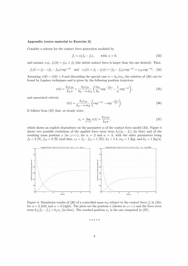
which shows an explicit dependence on the parameter α of the contact force model (33). Figure 4shows two possible evolutions of the applied force error term kf (fd − fc) (in blue) and of theresulting mass position x (in green), for α = 2 and α = 3, with the other parameters beingfd = 3 [N], fc0 = 2 [N] (and thus, ef = fd− fc0 = 1 [N]), kf = 1.4, md = 1 [kg], and kd = 1 [kg/s].

0 1 2 3 4 5 60

0.2

0.4

0.6

0.8

1

1.2

1.4

time [s]

scal

ed fo

rce

erro

r [N

] and

pos

ition

[m]

response for alfa = 2, fc0 = 2, fd = 3, kf = 1.4, md = 1, kd = 1 ==> xe =0.7

0 1 2 3 4 5 60

0.2

0.4

0.6

0.8

1

1.2

1.4

time [s]

scal

ed fo

rce

erro

r [N

] and

pos

ition

[m]

response for alfa = 3, fc0 = 2, fd = 3, kf = 1.4, md = 1, kd = 1 ==> xe =0.46667

Figure 4: Simulation results of (26) of a controlled mass md subject to the contact force fc in (34),for α = 2 [left] and α = 3 [right]. The plots are the position x (shown in green) and the force errorterm kf (fd − fc) = kfef (in blue). The reached position xe is the one computed in (37).

∗ ∗ ∗ ∗ ∗

8