robotic motion compensation for 3d ultrasound-guided...
TRANSCRIPT

Robotic Motion Compensation for
3D Ultrasound-Guided Beating Heart Surgery
A dissertation presented
by
Shelten Gee Jao Yuen
to
The School of Engineering and Applied Sciences
in partial fulfillment of the requirements
for the degree of
Doctor of Philosophy
in the subject of
Engineering Sciences
Harvard University
Cambridge, Massachusetts
September 2009

c©2009 - Shelten Gee Jao Yuen
All rights reserved.

Thesis advisor Author
Robert D. Howe Shelten Gee Jao Yuen
Robotic Motion Compensation for
3D Ultrasound-Guided Beating Heart Surgery
Abstract
Beating heart surgeries offer significant health benefits to patients by removing
the need for the heart-lung machine and its attendant side effects. These surgeries
are challenging to perform and only feasible in certain types of procedures because
of the rapid movement of the heart. Equipping the surgeon with fast, actuated,
and intelligent surgical instruments that automatically compensate for heart motion
could facilitate the execution of existing beating heart procedures and enable the
development of new procedures that are currently not possible. These tools have
particular promise for intracardiac beating heart procedures, where passive tissue
stabilization techniques are not available; however, achieving motion compensation
in this setting is challenging because of the sensing and space restrictions imposed
from working inside of the beating heart.
This thesis investigates 3D ultrasound-guided robotic motion compensation as an
assistive technology to intracardiac beating heart surgery. A number of engineering
challenges are addressed to develop a viable system for in vivo experimentation: heart
motion prediction to counter time delays in 3D ultrasound imaging and image pro-
cessing, real-time tracking of surgical targets in noisy 3D ultrasound images, and safe
iii
Abstract iv
force control schemes for the manipulation of tissue without exciting vibratory modes
in the robot. Solutions are provided in the form of a quasiperiodic extended Kalman
filter, a synergistic “flashlight” tissue tracker, and a force controller with feed-forward
target motion information, respectively. Integrating these components into a system,
motion compensation within the beating heart is not only shown to be feasible under
in vivo conditions, but also to provide significant performance advantages in beating
heart tasks. Motion and force tracking accuracies of 1.0 mm and 0.11 N are obtained
in in vivo surgical tasks with the system, constituting a 70% and 75% reduction in
error when compared to human performance in the same tasks.

Contents
Title Page . . . . . . . . . . . . . . . . . . . . . . . . . . . . . . . . . . . . iAbstract . . . . . . . . . . . . . . . . . . . . . . . . . . . . . . . . . . . . . iiiTable of Contents . . . . . . . . . . . . . . . . . . . . . . . . . . . . . . . . vAcknowledgments . . . . . . . . . . . . . . . . . . . . . . . . . . . . . . . . viiDedication . . . . . . . . . . . . . . . . . . . . . . . . . . . . . . . . . . . . ix
1 Introduction 1
1.1 Mitral Valve Annuloplasty . . . . . . . . . . . . . . . . . . . . . . . . 31.2 3D Ultrasound Guidance . . . . . . . . . . . . . . . . . . . . . . . . . 51.3 System Concept . . . . . . . . . . . . . . . . . . . . . . . . . . . . . . 61.4 Thesis Contributions . . . . . . . . . . . . . . . . . . . . . . . . . . . 81.5 Thesis Outline . . . . . . . . . . . . . . . . . . . . . . . . . . . . . . . 8
2 Time Delay Compensation 11
2.1 Mitral Valve Annulus Motion . . . . . . . . . . . . . . . . . . . . . . 142.2 Motion Compensation Instrument . . . . . . . . . . . . . . . . . . . . 172.3 Heart Motion Prediction . . . . . . . . . . . . . . . . . . . . . . . . . 20
2.3.1 Predictive Filters . . . . . . . . . . . . . . . . . . . . . . . . . 212.3.2 Simulation Studies . . . . . . . . . . . . . . . . . . . . . . . . 27
2.4 Performance Evaluation in a Surgical Task . . . . . . . . . . . . . . . 322.4.1 Experimental Setup . . . . . . . . . . . . . . . . . . . . . . . . 322.4.2 User Task . . . . . . . . . . . . . . . . . . . . . . . . . . . . . 332.4.3 Independent Variables . . . . . . . . . . . . . . . . . . . . . . 352.4.4 Testing Protocol . . . . . . . . . . . . . . . . . . . . . . . . . 382.4.5 Results . . . . . . . . . . . . . . . . . . . . . . . . . . . . . . . 39
2.5 System Accuracy Under 3D Ultrasound Guidance . . . . . . . . . . . 452.5.1 Experimental Setup . . . . . . . . . . . . . . . . . . . . . . . . 452.5.2 Results . . . . . . . . . . . . . . . . . . . . . . . . . . . . . . . 47
2.6 Discussion . . . . . . . . . . . . . . . . . . . . . . . . . . . . . . . . . 47
v

Contents vi
3 Real-Time Tissue Tracking 53
3.1 3D Ultrasound-Guided Motion Compensation System . . . . . . . . . 553.1.1 Real-Time 3D Ultrasound “Flashlight” Tissue Tracker . . . . 563.1.2 Time Delay Compensation . . . . . . . . . . . . . . . . . . . . 573.1.3 Motion Compensation Instrument . . . . . . . . . . . . . . . . 583.1.4 System Implementation . . . . . . . . . . . . . . . . . . . . . 59
3.2 Water Tank Validation . . . . . . . . . . . . . . . . . . . . . . . . . . 603.2.1 Experimental Setup . . . . . . . . . . . . . . . . . . . . . . . . 613.2.2 Testing Protocol . . . . . . . . . . . . . . . . . . . . . . . . . 613.2.3 Results . . . . . . . . . . . . . . . . . . . . . . . . . . . . . . . 63
3.3 In Vivo Animal Study . . . . . . . . . . . . . . . . . . . . . . . . . . 653.3.1 Experimental Setup . . . . . . . . . . . . . . . . . . . . . . . . 653.3.2 Results . . . . . . . . . . . . . . . . . . . . . . . . . . . . . . . 67
3.4 Discussion . . . . . . . . . . . . . . . . . . . . . . . . . . . . . . . . . 70
4 Force Tracking with Feed-Forward Motion Estimation 74
4.1 Rigid Body Analysis . . . . . . . . . . . . . . . . . . . . . . . . . . . 774.2 Bandwidth Contraints due to Robot Dynamics . . . . . . . . . . . . . 81
4.2.1 Gain Limit to Avoid Vibration . . . . . . . . . . . . . . . . . 834.2.2 Experimentally Observed Vibration and Instability . . . . . . 86
4.3 Force Control with Feed-Forward Target Motion . . . . . . . . . . . . 914.4 Tissue Motion Estimation with 3D Ultrasound . . . . . . . . . . . . . 924.5 In Vivo System Validation . . . . . . . . . . . . . . . . . . . . . . . . 94
4.5.1 Experimental Setup . . . . . . . . . . . . . . . . . . . . . . . . 944.5.2 Results . . . . . . . . . . . . . . . . . . . . . . . . . . . . . . . 96
4.6 Discussion . . . . . . . . . . . . . . . . . . . . . . . . . . . . . . . . . 98
5 Conclusions and Future Work 101
5.1 Conclusions . . . . . . . . . . . . . . . . . . . . . . . . . . . . . . . . 1025.2 Future Directions . . . . . . . . . . . . . . . . . . . . . . . . . . . . . 106
Bibliography 110

Acknowledgments
I am fortunate and honored to be surrounded by so many supportive, motivated,
and brilliant people. This work would not have been possible without them and I
would like to extend my heartfelt thanks for their help.
First and foremost I want to thank my advisor Professor Robert Howe. He has
always pushed me toward the big problems while giving me the freedom to solve them
in my own way. I could not have asked for or imagined a better guide through the
Ph.D. process and I truly appreciate the time and effort that he spent teaching me.
I also want to thank my committee members Dr. Pedro del Nido, Professor Pierre
Dupont, and Professor Robert Wood for their insight and direction on this thesis
from start to finish.
The members of the Biorobotics Lab have shared with me the joys and travails of
graduate research. They have shaped my thinking and, without fail, given me those
well-timed nudges of encouragement to keep me going. I give my thanks to Ryan
Beasley, Aaron Dollar, Yuri Ishihara, Leif Jentoft, Amy Kerdok, Marius Linguraru,
Masashi Nakatani, Riichiro Tadakuma, Mahdi Tavakoli, and Chris Wagner for their
help throughout. The majority of my work was done in collaboration with members
from the lab: Paul Novotny, Daniel Kettler, Samuel Kesner, Michael Yip, and Alex
Dubec. It was a pleasure working with them and I am deeply grateful for their efforts
and insights, without which I could not have achieved so much so quickly. Finally,
I want to especially thank Petr Jordan, Peter Hammer, Douglas Perrin, and Robert
Schneider for not only spending countless hours brainstorming with me, but also for
their kind friendship.
I have had the privilege of working with the finest cardiac surgeons in the world
vii
Acknowledgments viii
at Children’s Hospital Boston. Dr. Pedro del Nido, Dr. Nikolay Vasilyev, and Dr.
Mitsuhiro Kawata have all lended their time and immense medical expertise toward
this thesis, to which I am thankful. In particular, Dr. Vasilyev performed all of the in
vivo surgical experiments in this thesis and, in conjunction with Dr. Douglas Perrin,
helped me to advance this project at every phase. I am indebted to both of them
for their feedback, paper edits, and patience. I also want to thank Hugo Loyola for
always being up to unwind over a cup of coffee with me while I worked at Children’s.
I cannot stress enough the importance of my nurturing family: Allan Yuen, So San
Aldridge, Stephen Aldridge, and Chris Yuen. They taught me how to think critically,
work hard, live generously, and be happy. My accomplishments are a testament to
their work in me.
Finally, I would like to thank my extraordinary wife Priscilla. She has contributed
to every aspect of this thesis as an experimenter, test subject, and editor. I would
not have survived and succeeded without her. I thank her for the wonderful gifts that
she has given to me in unwavering love, support, and our beautiful daughter Elsie.

For Priscilla
ix
Chapter 1
Introduction
Beating heart surgery is a promising and, in many cases, preferred alternative to
conventional cardiac surgery. In this surgical approach, the surgeon operates on the
heart while it pumps and, in doing so, circumvents many of the serious side effects for
patients that occur as a result of stopping the heart and using the heart-lung machine.
These side effects include increased risk of stroke [54], inflammatory response [8], and
long-term neurocognitive dysfunction [43]. Beating heart procedures have shown
a significant reduction of risk for these side effects [41], while also decreasing the
postoperative recovery time in the hospital by 13% [3] and overall medical cost by 20–
30% [41, 3]. Beating heart procedures also allow the surgeon to evaluate the surgery
under physiologic loading conditions. This is useful in the repair of structures like the
mitral valve that open and close in response to changing pressure gradients during
the heart cycle [23].
The advantages of beating heart procedures are not obtained easily: surgical
manipulation presents a significant challenge to the surgeon because cardiac motions
1

Chapter 1: Introduction 2
are too fast for humans to track by hand [18, 32]. As an example, the mitral valve
annulus traverses most of its trajectory and undergoes three direction changes in
about a tenth of a second [37], making it difficult for the surgeon to execute the
precise surgical maneuvers required for tasks like mitral valve annuloplasty. Recent
animal trials indicate that beating heart modification of the mitral valve cannot be
performed reliably due to its fast motion [15].
For certain types of procedures, heart motion can be restrained with a passive
mechanical stabilizer attached to the heart surface. This approach has enabled the
widespread use of beating heart techniques in coronary artery bypass graft proce-
dures (18% to 20% in the United States [41]). However, passive stabilization is an
imperfect solution. Its use can damage the heart [64] and tissue constrained in this
manner still exhibits significant residual motion [40]. Furthermore, stabilizers can
only be used on the top surface of the heart and so are not applicable to many types
of procedures, such as the broad category of those performed inside of the heart called
intracardiac procedures.
The limitations of passive stabilization have inspired the development of active
robotic tools that move with the heart. This is referred to as motion compensation.
Current research shows a great deal of promise for this approach. In two controlled
laboratory experiments, the use of a moving hand support [64] or an actuated, hand-
held surgical instrument [37] increased accuracy by 80% and 50% (respectively) in
simulated beating heart surgical tasks. Inside of the operating room, a robot has
shown tracking accuracies on the order of 2 mm following the complex motion of the
external heart wall [24]. A number of other studies have shown that heart motion can

Chapter 1: Introduction 3
be accurately predicted and followed by a robot in vitro [44, 62, 51, 6, 21, 5, 22, 4].
Previous research has focused on coronary artery bypass graft in order to improve
an existing beating heart procedure. However, robotic motion compensation has the
potential to act as an enabling technology for the development of new beating heart
procedures that are not currently possible. It is of interest to determine if motion
compensation can be achieved in the intracardiac setting, where passive stabilizers
are not useful and there are stringent sensing and space restrictions. This thesis will
show that motion compensation can be achieved inside the heart using standard 3D
ultrasound imaging for guidance. Mitral valve annuloplasty is chosen as a specific
surgical application for in vivo experimental validation because it is currently outside
the reach of beating heart procedures. Furthermore, while previous research in motion
compensation have achieved impressive position tracking results, there is no evidence
that it affords any benefit to the surgeon in the operating room. This thesis will
demonstrate that motion compensation enhances in vivo surgical task performance.
1.1 Mitral Valve Annuloplasty
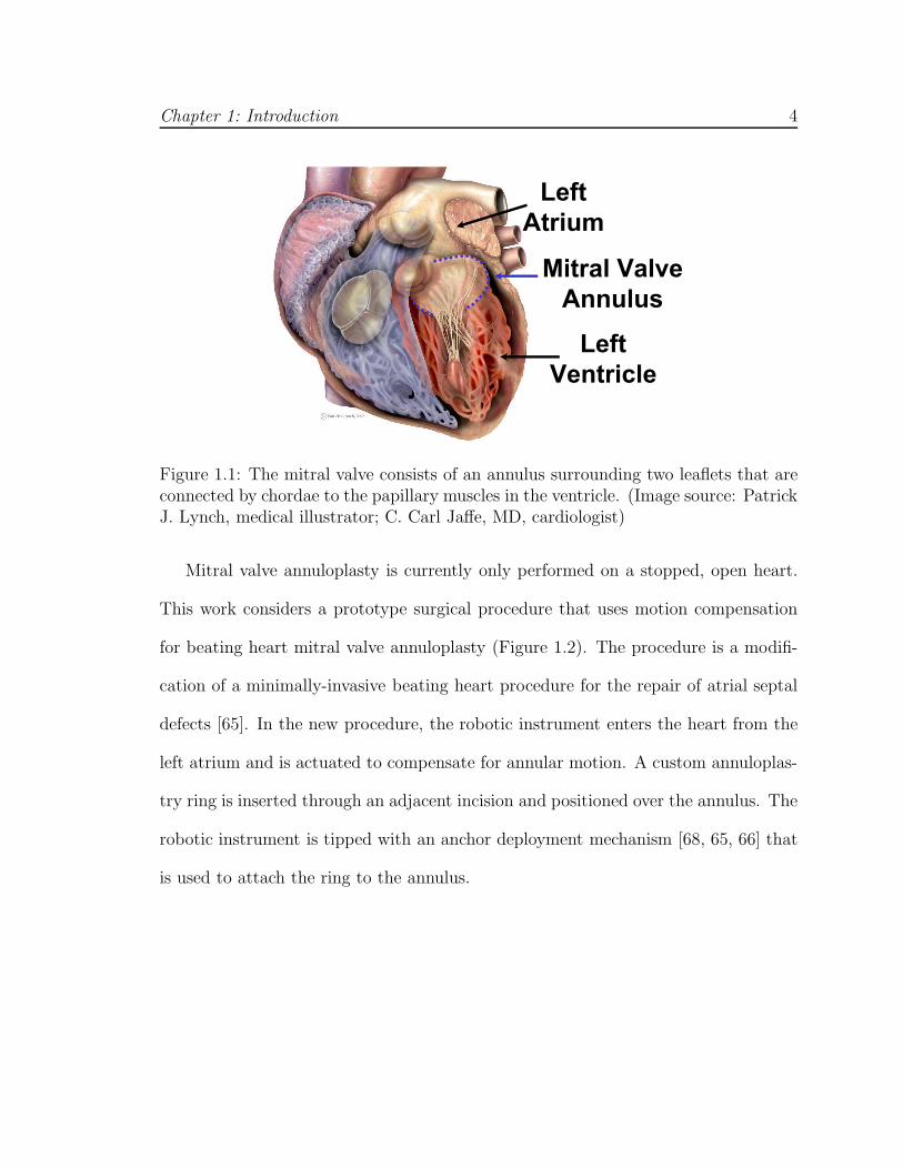
The mitral valve (Figure 1.1) is a structure that is critical for the correct, uni-
directional flow of oxygenated blood from the lungs to the body. An incompetent
(i.e., leaky) valve can cause severe symptoms in the patient ranging from arrhythmia
to heart failure. In the repair of an incompetent mitral valve, a synthetic ring is
attached to the junction between the annulus and the atrial wall. This procedure,
called mitral valve annuloplasty, attempts to reduce the annulus shape to that of the
synthetic annuloplasty ring so that the leaflets meet properly.
Chapter 1: Introduction 4
Mitral Valve
Annulus
Left
Ventricle
Left
Atrium
Figure 1.1: The mitral valve consists of an annulus surrounding two leaflets that areconnected by chordae to the papillary muscles in the ventricle. (Image source: PatrickJ. Lynch, medical illustrator; C. Carl Jaffe, MD, cardiologist)
Mitral valve annuloplasty is currently only performed on a stopped, open heart.
This work considers a prototype surgical procedure that uses motion compensation
for beating heart mitral valve annuloplasty (Figure 1.2). The procedure is a modifi-
cation of a minimally-invasive beating heart procedure for the repair of atrial septal
defects [65]. In the new procedure, the robotic instrument enters the heart from the
left atrium and is actuated to compensate for annular motion. A custom annuloplas-
try ring is inserted through an adjacent incision and positioned over the annulus. The
robotic instrument is tipped with an anchor deployment mechanism [68, 65, 66] that
is used to attach the ring to the annulus.

Chapter 1: Introduction 5
Annuloplasty
Ring Holder
Left
Atrium
Anchor Driver
Figure 1.2: Prototype beating heart mitral valve annuloplasty procedure using roboticmotion compensation instrumentation.
1.2 3D Ultrasound Guidance
A major consideration for intracardiac robot control is how the robot will be
guided. The motion compensation system in this work uses 3D ultrasound imaging
because it is capable of imaging through blood and it provides more spatial informa-
tion to guide complex intracardiac procedures than traditional 2D ultrasound [10].
While other imaging modalities like 3D computed tomography and magnetic reso-
nance imaging offer higher spatial resolution, they have prohibitively slow imaging
speeds, require special facilities, incur high costs, and cannot be moved into the
operating room. In contrast, 3D ultrasound is relatively cheap, portable, and oper-
ates in real-time (24–30 Hz). 3D ultrasound is also becoming the preferred imag-
ing technology among cardiac surgeons for guiding intracardiac beating heart re-
pairs [61, 60, 65, 66] and it is advantageous to use it in the system to reduce training.

Chapter 1: Introduction 6
Despite its advantages, there are a number of difficulties associated with using 3D
ultrasound for robotic motion compensation. It has high noise, poor shape definition,
and imaging artifacts that can distort the appearance of tissues and instruments [30].
Novotny et al. found that accurate, real-time instrument tracking could be achieved
in vivo by exploiting the high spatial coherence of surgical instruments in 3D ultra-
sound [48]. Subsequently, a robot could be visually servoed to mimic heart motion
in vitro, although with a large 130 ms temporal lag that is unacceptable for in vivo
motion compensation [46]. The lag was attributed to delays in the acquisition, trans-
fer, and processing of 3D ultrasound volumes as well as robot latency [46].
This previous research indicates that a number of interesting and unsolved prob-
lems must be addressed to use 3D ultrasound for robot guidance. Methods are re-
quired to automatically track in vivo surgical targets in noisy 3D ultrasound while
compensating for the time delays present in both the imaging and the robot. In this
work, solutions are provided to address these problems.
1.3 System Concept
The 3D ultrasound-guided motion compensation system proposed in this work
partners the medical expertise of the surgeon with the speed of a robot to augment
the capabilities of the surgeon in beating heart procedures. Figure 1.3 illustrates the
general system concept. The surgeon holds a robotic instrument, navigates it to the
surgical site, and designates the surgical target by pointing the instrument tip toward
it. A set of automated algorithms determine the position of the surgical target in
3D ultrasound and are used to command the robot. Because the robot utilizes the
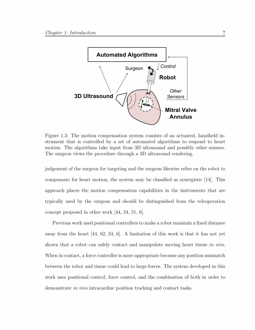
Chapter 1: Introduction 7
Robot
3D Ultrasound
Mitral Valve
Annulus
Automated Algorithms
Surgeon Control
Other
Sensors
Figure 1.3: The motion compensation system consists of an actuated, handheld in-strument that is controlled by a set of automated algorithms to respond to heartmotion. The algorithms take input from 3D ultrasound and possibly other sensors.The surgeon views the procedure through a 3D ultrasound rendering.
judgement of the surgeon for targeting and the surgeon likewise relies on the robot to
compensate for heart motion, the system may be classified as synergistic [14]. This
approach places the motion compensation capabilities in the instruments that are
typically used by the surgeon and should be distinguished from the teleoperation
concept proposed in other work [44, 24, 51, 6].
Previous work used positional controllers to make a robot maintain a fixed distance
away from the heart [44, 62, 24, 6]. A limitation of this work is that it has not yet
shown that a robot can safely contact and manipulate moving heart tissue in vivo.
When in contact, a force controller is more appropriate because any position mismatch
between the robot and tissue could lead to large forces. The system developed in this
work uses positional control, force control, and the combination of both in order to
demonstrate in vivo intracardiac position tracking and contact tasks.
Chapter 1: Introduction 8
1.4 Thesis Contributions
This thesis demonstrates for the first time the in vivo feasibility and performance
advantages of robotic motion compensation for intracardiac beating heart surgical
tasks. To do this, a 3D ultrasound-guided robotic motion compensation system is
developed. The system incorporates the robot design of Kettler et al. [37] and real-
time 3D ultrasound instrument tracking algorithm of Novotny et al. [48].
There are several interesting challenges to overcome in the development of the
system. The time delays and noise inherent to 3D ultrasound [46] must be addressed
for the real-time guidance of a robot in vivo. Furthermore, the structural dynamics
of the robot are an obstacle to safe control when in contact with moving tissue. This
work provides solutions to these challenges by drawing on methods from the fields of
estimation, image processing, and control. The major technological contributions are
the development of a predictive heart motion filtering method to mitigate noise and
time delay in 3D ultrasound; the development of a synergistic approach to real-time
3D ultrasound tissue tracking for in vivo robot guidance; and the development of a
robotic force tracking system that incorporates feed-forward motion information for
beating heart tissue manipulation.
1.5 Thesis Outline
This thesis is presented as a set of successive technology advancements that are
needed to realize a 3D ultrasound-guided motion compensation system.
Chapter 2 addresses the challenge of accurately estimating heart motion to servo

Chapter 1: Introduction 9
a robotic instrument when provided noisy, time-delayed positional information by 3D
ultrasound. This chapter proposes the use of an extended Kalman filter that explicitly
models heart rate variability and sensor noise to increase estimate accuracy. This
method is shown to provide more accurate estimates than existing techniques through
computer simulation and in vitro experiments. Subsequent user testing in an in vitro
surgical task demonstrates that the extended Kalman filter restores the performance
benefits of motion compensation that are lost when there is uncompensated time
delay.
Chapter 3 introduces a novel, real-time 3D ultrasound tissue tracking algorithm
adapted for cardiac structures that undergo primarily uniaxial motion. The mitral
valve annulus is an example of such a structure [37]. The algorithm is robust to
imaging noise because it draws on the high spatial coherence of the instrument in
3D ultrasound to locate the tissue target. Integrating this algorithm with the filter
from Chapter 2 results in a motion tracking system suitable for mitral valve annulo-
plasty. In vitro and in vivo experiments with this system demonstrate the positioning
accuracy and task performance enhancement conferred in beating heart procedures.
Chapter 4 solves the problem of applying precise forces against a fast-moving car-
diac target during surgical manipulation by incorporating a force controller into the
system. Analysis and experiments are presented to show that current surgical instru-
ments impose stringent bandwidth limitations that preclude accurate force tracking
with a standard force controller. A feed-forward force control strategy is proposed
that incorporates the motion filtering and tracking algorithms from Chapters 2 and 3.
The resulting system is validated under in vivo conditions and shown to significantly

Chapter 1: Introduction 10
reduce force fluctuations when compared to manual attempts to maintain a constant
force against the mitral valve annulus.
Chapter 5 discusses the implications of this research on motion compensation and
intracardiac beating heart surgery. While the technologies developed in this work
focus on mitral valve annuloplasty, they have wider applicability to other procedures
both inside and outside of the heart. Future enhancements to the work are also
outlined.

Chapter 2
Time Delay Compensation
Real-time 3D ultrasound is an effective imaging technology for surgical guidance
within the beating heart. Cannon et al. demonstrated that the increased spatial
information provided by 3D ultrasound enables the execution of complex tasks that
are not possible with traditional 2D ultrasound [10] and recently surgeons have shown
that 3D ultrasound can be used to guide the closure of atrial septal defects [61, 60, 65]
and ventricular septal defects [66] in the beating heart. These studies suggest that 3D
ultrasound is a good candidate for guiding a motion compensation system for beating
heart surgery, both because it has the speed, fidelity, and spatial information to guide
surgery on moving cardiac structures and because it is currently used by and familiar
to surgeons. However, there are delays of approximately 60 ms inherent to using 3D
ultrasound that can cause a motion compensation system to lag behind fast-moving
heart structures [46] – in effect, not compensating for heart motion at all.
Latency is intrinsic to every robotic system and can arise from a number of sources.
One fundamental source is inertia: regardless of how fast the robot moves, it takes
11
Chapter 2: Time Delay Compensation 12
finite time to respond to a commanded input. When the inertia of the robot is
large relative to its actuation capabilities, the associated latency will be large. This
has been one of the main challenges addressed in previous research in extracardiac
motion compensation for coronary artery bypass graft procedures, where relatively
large, multiple degree of freedom (DOF) robots track the external surface of the heart
wall [24, 6]. In that work, researchers exploited the nearly periodic motion of the heart
to feed-forward a trajectory into a model predictive controller so that the effective
tracking bandwidth of the robot was increased. Ginhoux et al. first showed that this
strategy could achieve robot tracking errors of approximately 1.5 mm on a beating
porcine heart using a high speed camera to observe heart motion (500 Hz sampling
rate, 330 µm accuracy) and then predicting heart motion into the near future with
an adaptive harmonic filter bank [24]. In independent work, Bebek and Cavusoglu
demonstrated less than 1 mm robot tracking error by using ECG and the previous
heart cycle trajectory to predict motion in the next heart cycle [6]. Their system
used sonomicrometry sensors sutured to the surface of a porcine heart, sampling at
257 Hz with 250 µm position accuracy. These studies indicate that the predictability
of heart motion can be used to overcome system latency when fast, high accuracy
sensors are employed for guidance.
In this chapter, we show that a similar approach can be used to overcome delays
in a 3D ultrasound-guided motion compensation system where the delays are primar-
ily due to imaging. There are several new aspects to the problem of heart motion
prediction in this setting. Unlike the sensors used in the previous work, 3D ultra-
sound has a relatively low sampling rate (24–30 Hz), low resolution (approximately
Chapter 2: Time Delay Compensation 13
Delay-Compensated
Target Position Estimates
Motion
Compensation
Instrument
3D Ultrasound Imaging
and Target SegmentationMitral Valve
Annulus
Robot
Controller
Control Signal
Predictive Filter
Delayed Target
Position
Measurements
Surgeon
Display
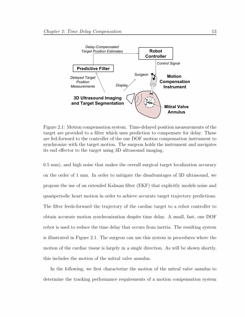
Figure 2.1: Motion compensation system. Time-delayed position measurements of thetarget are provided to a filter which uses prediction to compensate for delay. Theseare fed-forward to the controller of the one DOF motion compensation instrument tosynchronize with the target motion. The surgeon holds the instrument and navigatesits end effector to the target using 3D ultrasound imaging.
0.5 mm), and high noise that makes the overall surgical target localization accuracy
on the order of 1 mm. In order to mitigate the disadvantages of 3D ultrasound, we
propose the use of an extended Kalman filter (EKF) that explicitly models noise and
quasiperiodic heart motion in order to achieve accurate target trajectory predictions.
The filter feeds-forward the trajectory of the cardiac target to a robot controller to
obtain accurate motion synchronization despite time delay. A small, fast, one DOF
robot is used to reduce the time delay that occurs from inertia. The resulting system
is illustrated in Figure 2.1. The surgeon can use this system in procedures where the
motion of the cardiac tissue is largely in a single direction. As will be shown shortly,
this includes the motion of the mitral valve annulus.
In the following, we first characterize the motion of the mitral valve annulus to
determine the tracking performance requirements of a motion compensation system

Chapter 2: Time Delay Compensation 14
for mitral valve annuloplasty. Next, we describe the actuated, one DOF robot that
we term the motion compensation instrument. We then describe the EKF and several
other predictive filtering methods and compare them in simulation. Two subsequent
user studies evaluate the benefit of a motion compensation system against traditional
non-tracking tools in a simulated in vitro surgical task. Furthermore, they validate
the robustness that the EKF provides to the system in situations of high noise, time
delay, and heart rate variability. Finally, we measure the position tracking accuracy of
the system in a series of 3D ultrasound-guided motion synchronization experiments.
The mitral valve annulus motion, motion compensation instrument, and first user
study were first described in [37] and are included in this chapter for clarity and
completeness.
2.1 Mitral Valve Annulus Motion
To guide the development of a motion compensation system for mitral valve an-
nuloplasty, the motion of the mitral valve annulus was analyzed using ultrasound
image data like that available in surgery for real-time guidance. A transthoracic 3D
ultrasound image-volume sequence of the mitral valve annulus was acquired at 24 Hz
(SONOS 7500, Philips Healthcare, Andover, MA, USA). This raw 3D ultrasound
data was manually segmented to extract mitral valve annulus trajectory information.
For each 3D volume sample, a minimum of 50 data points were selected from the
mitral valve annulus and used to locate the annulus centroid. Repeated for each
time-stamped data frame, this process generated a record of the annulus centroid
position over the cycle of the heartbeat. Because this manual segmentation process
Chapter 2: Time Delay Compensation 15
0 0.2 0.4 0.6 0.8 1 1.2 1.4−10
−5
0
5
10
Time (s)
Pos
ition
(m
m)
1st Component2nd Component3rd Component
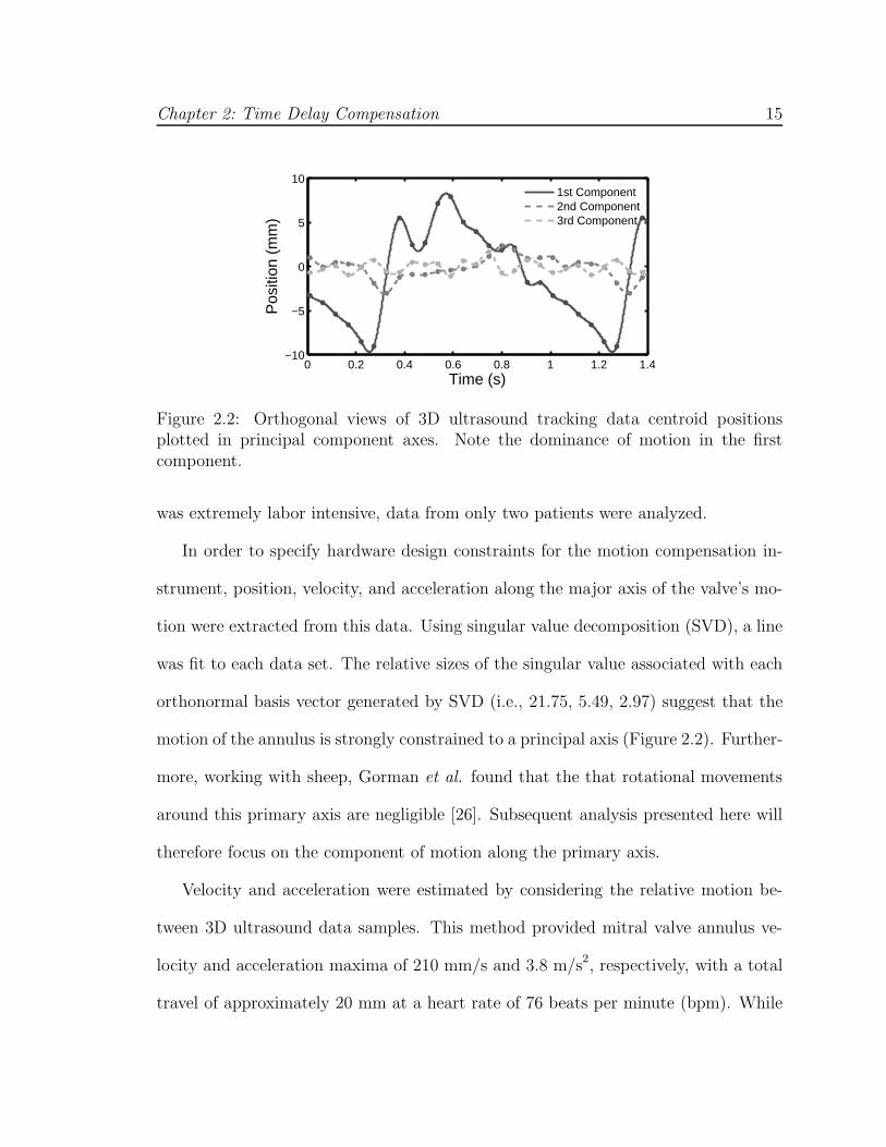
Figure 2.2: Orthogonal views of 3D ultrasound tracking data centroid positionsplotted in principal component axes. Note the dominance of motion in the firstcomponent.
was extremely labor intensive, data from only two patients were analyzed.
In order to specify hardware design constraints for the motion compensation in-
strument, position, velocity, and acceleration along the major axis of the valve’s mo-
tion were extracted from this data. Using singular value decomposition (SVD), a line
was fit to each data set. The relative sizes of the singular value associated with each
orthonormal basis vector generated by SVD (i.e., 21.75, 5.49, 2.97) suggest that the
motion of the annulus is strongly constrained to a principal axis (Figure 2.2). Further-
more, working with sheep, Gorman et al. found that the that rotational movements
around this primary axis are negligible [26]. Subsequent analysis presented here will
therefore focus on the component of motion along the primary axis.
Velocity and acceleration were estimated by considering the relative motion be-
tween 3D ultrasound data samples. This method provided mitral valve annulus ve-
locity and acceleration maxima of 210 mm/s and 3.8 m/s2, respectively, with a total
travel of approximately 20 mm at a heart rate of 76 beats per minute (bpm). While

Chapter 2: Time Delay Compensation 16
Figure 2.3: 3D ultrasound tracking data spectral decomposition. Note that the am-plitudes quickly decrease with increasing frequency.
only two subjects were analyzed in this fashion, work by Kamigaki and Goldschlager
on the mitral valve leaflets reports similar velocity and amplitude results [35].
Figure 2.3 shows the spectral decomposition of the major axis motion trajectory.
The dominant motion components are at 1.3, 2.6, and 5.2 Hz, with further components
of decreasing amplitude at higher frequencies. This is consistent with the findings of
Nakamura et al. which show dominant frequency components of 1.5 Hz and 3.0 Hz
in the motion of porcine epicardium [44]. Ginhoux et al. found the same major
frequency components in the motion of porcine epicardium [24]. This paper also
noted higher frequency transients that it deemed significant and concluded that a
25 Hz sampling rate would be insufficient to track the motion of the epicardium with
high precision [24]. Bebek and Cavusoglu found similar frequency components, but
concluded that the motion could be adequately characterized using lower sampling
frequencies (i.e., 26 Hz) [6].

Chapter 2: Time Delay Compensation 17
2.2 Motion Compensation Instrument
Prior work on beating heart motion compensation has largely focused on the use of
multiple DOF teleoperated manipulators for extracardiac procedures. Implementing a
full six DOF robot for intracardiac applications has a number of challenges, including
the development of a manipulator with sufficient mechanical bandwidth, creating
a wrist that can operate in the restricted workspace within the beating heart, and
ensuring safety for a complex manipulator system. These requirements are far beyond
the capabilities of current commercial surgical robots.
Rather than attempting to correct for motion components in all three dimensions,
we propose a robot that compensates for the major component of motion and allows
the surgeon and passive tissue compliance to counter the slow or relatively minor
motions along the remaining two axes. The robot, called the motion compensation
instrument (MCI), is an actuated, handheld instrument that aids the surgeon in work-
ing on the moving mitral valve. It is adapted for the prototype procedure described in
Chapter 1. The instrument is inserted through the left atrial appendage and aimed
toward the mitral valve annulus, which is also along the major motion axis of the
annulus (Figure 1.2).
The selection of the mechanical mechanism to follow the linear motion compo-
nent of the mitral valve annulus was guided by the clinical 3D ultrasound trajectory
analysis from Section 2.1. The high velocity and acceleration requirements lead to
a linear motor based design which benefits from low friction and low moving mass
(Figure 2.4). This design format also produces a surgical tool similar in design and
function to typical endoscopic tools, supported by a port and maneuvered by hand.
Chapter 2: Time Delay Compensation 18
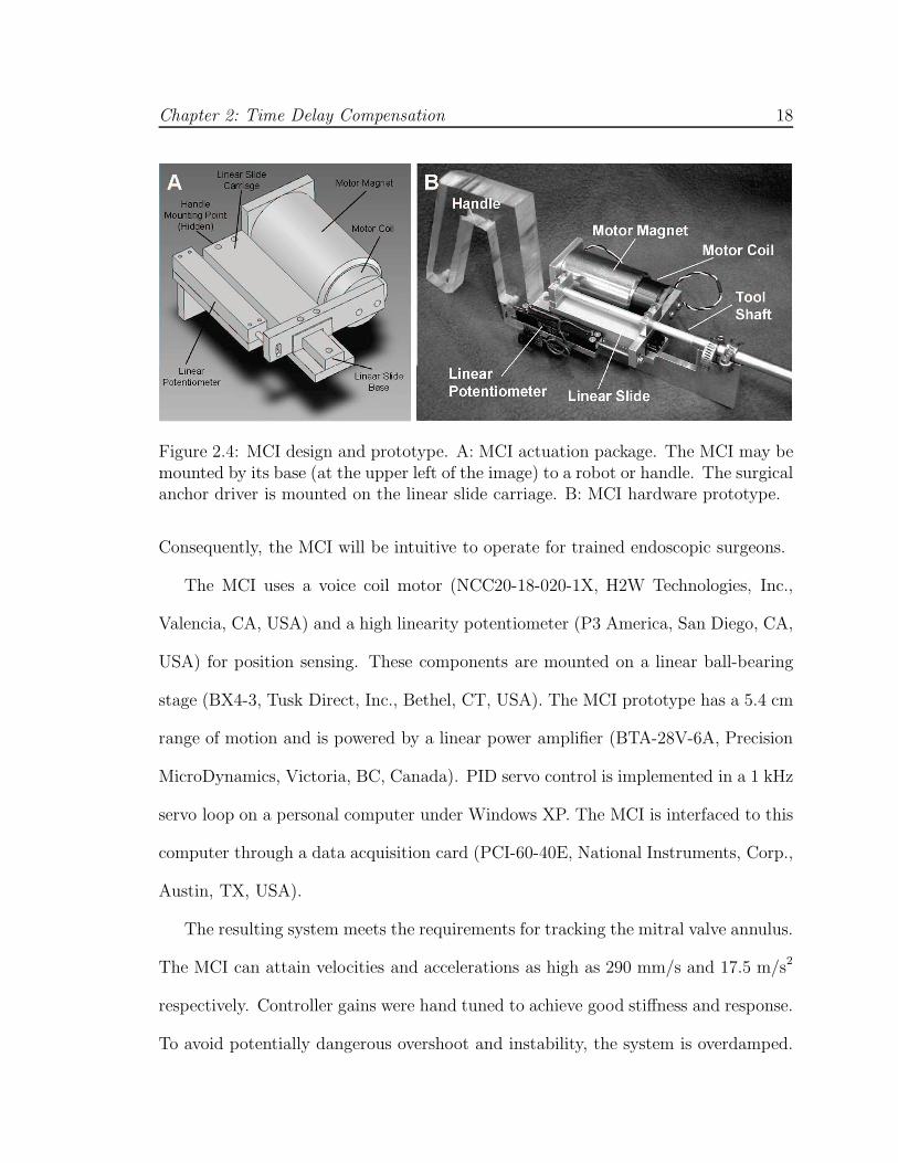
Figure 2.4: MCI design and prototype. A: MCI actuation package. The MCI may bemounted by its base (at the upper left of the image) to a robot or handle. The surgicalanchor driver is mounted on the linear slide carriage. B: MCI hardware prototype.
Consequently, the MCI will be intuitive to operate for trained endoscopic surgeons.
The MCI uses a voice coil motor (NCC20-18-020-1X, H2W Technologies, Inc.,
Valencia, CA, USA) and a high linearity potentiometer (P3 America, San Diego, CA,
USA) for position sensing. These components are mounted on a linear ball-bearing
stage (BX4-3, Tusk Direct, Inc., Bethel, CT, USA). The MCI prototype has a 5.4 cm
range of motion and is powered by a linear power amplifier (BTA-28V-6A, Precision
MicroDynamics, Victoria, BC, Canada). PID servo control is implemented in a 1 kHz
servo loop on a personal computer under Windows XP. The MCI is interfaced to this
computer through a data acquisition card (PCI-60-40E, National Instruments, Corp.,
Austin, TX, USA).
The resulting system meets the requirements for tracking the mitral valve annulus.
The MCI can attain velocities and accelerations as high as 290 mm/s and 17.5 m/s2
respectively. Controller gains were hand tuned to achieve good stiffness and response.
To avoid potentially dangerous overshoot and instability, the system is overdamped.

Chapter 2: Time Delay Compensation 19
Figure 2.5: Frequency response of the MCI. Note that the system is overdamped andhas a -3 dB point of 20.6 Hz.
The tool has a static stiffness of 0.23 N/mm and a friction force less than 0.009 N.
The system’s frequency response is similarly adequate for the tracking task (Figure
2.5). The system has a -3 dB point of 20.6 Hz and roll off rate of 40 dB per decade.
The potentiometer on the MCI measures position with a root mean square (RMS)
error of less than 0.01 mm. The system is capable of maintaining stationary at a
commanded position with a RMS error of 0.009 mm.
The tracking abilities of the MCI were demonstrated by commanding the system to
follow the motion of a mitral valve at 60 bpm (Figure 2.6). Mitral annulus motion was
determined from the 3D ultrasound data in Figure 2.2. The MCI reliably replicated
the motion profile of the valve with an effective delay of 14 ms.
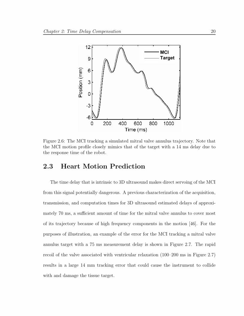
Chapter 2: Time Delay Compensation 20
MCI
Target
Figure 2.6: The MCI tracking a simulated mitral valve annulus trajectory. Note thatthe MCI motion profile closely mimics that of the target with a 14 ms delay due tothe response time of the robot.
2.3 Heart Motion Prediction
The time delay that is intrinsic to 3D ultrasound makes direct servoing of the MCI
from this signal potentially dangerous. A previous characterization of the acquisition,
transmission, and computation times for 3D ultrasound estimated delays of approxi-
mately 70 ms, a sufficient amount of time for the mitral valve annulus to cover most
of its trajectory because of high frequency components in the motion [46]. For the
purposes of illustration, an example of the error for the MCI tracking a mitral valve
annulus target with a 75 ms measurement delay is shown in Figure 2.7. The rapid
recoil of the valve associated with ventricular relaxation (100–200 ms in Figure 2.7)
results in a large 14 mm tracking error that could cause the instrument to collide
with and damage the tissue target.

Chapter 2: Time Delay Compensation 21
A B
Figure 2.7: MCI tracking of a mitral valve target with 75 ms measurement delay from3D ultrasound imaging and processing. A: MCI and target positions; B: Trackingerror. Note that the additional 14 ms response time of the MCI yields an effectivedelay of 89 ms. Max and RMS tracking errors are 14.49 and 4.60 mm, respectively.
2.3.1 Predictive Filters
To avoid this outcome, we exploit the near periodicity of the mitral valve annu-
lus trajectory to predict its path and hence compensate for time delay. However,
such predictions must be made in the presence of measurement noise and a poten-
tially variable heart rate. In this section we describe and evaluate several predictive
filtering methods that can be employed for delay compensation in this setting: an
autoregressive filter, a fading memory autoregressive filter, and an extended Kalman
filter (EKF) with a quasiperiodic motion model. The autoregressive filter has pre-
viously been applied by Nakamura et al. in a spectral analysis of heart motion for
motion compensation in coronary artery bypass graft (CABG) procedures [44]. In
principle, this method is equivalent to the adaptive harmonic filter bank used by Gin-
houx et al. for CABG [24] and has its attendant assumption of a fixed heart rate.
The fading memory autoregressive filter overcomes this limitation despite using the

Chapter 2: Time Delay Compensation 22
same model by exponentially discounting the measurements supplied to the filter,
thereby allowing it to adjust to more recent information. This approach has been
used for motion synchronization in CABG by Franke et al. [21]. In contrast, the EKF
permits variations to heart rate by directly accounting for it in a time-varying Fourier
series model. A similar model was employed by Riviere et al. in the Weighted Fourier
Linear Combiner (WFLC) estimator for CABG [53]; however, unlike the EKF, this
method does not explictly model noise. Ortmaier et al. has evaluated other nonlinear
prediction techniques for CABG such as artificial neural networks and an estimator
based on Takens theorem [51].
Autoregressive Filter
Fixed-rate mitral valve annulus motion can be modeled as an n-order autoregres-
sive (AR) process
y[k] =n∑
i=1
αiy[k − i], (2.1)
where αi, i ∈ {1, ..., n} are the model coefficients and y[k] is the target position at time
sample k. Note that rather than explicitly assuming periodicity in the target motion,
this model predicates that the kth position can be expressed as a linear combination
of the previous n positions.
In order to predict the target position, the model coefficients and order must
be estimated. The first can be achieved in real-time using the recursive covariance
method estimator. Denoting z[k] = y[k] + ν[k] to be the noise-corrupted position
measurement at time sample k with ν[k] ∼ N (0, σ2R), this estimator is expressed

Chapter 2: Time Delay Compensation 23
compactly in matrix form as
Z[k] = [z[k − n − 1], . . . , z[k − 1]]
R[k] = R[k − 1] + Z[k]TZ[k] (2.2)
α[k] = α[k − 1] + R[k]−1Z[k]T (z[k] − Zα[k − 1]) , (2.3)
with initial conditions R[0] = 0 and α[0] = 0. An appropriate autoregressive model
order was determined using the Akaike Information Criteria [11] on the mitral valve
annulus trajectory in Figure 2.2, yielding n = 30. Predicted target locations, y[k], can
be obtained through evaluation of Equation 2.1. Additionally, the target trajectory
can be interpolated from its inherent measurement rate (i.e., 28 Hz, a typical 3D
ultrasound frame rate) to the higher control rate of the robot using the Whittaker-
Shannon interpolation formula.
Fading Autoregressive Filter
Imperfect periodicity can cause the AR model coefficients to change over time. In
this situation, it can be useful to preferentially weight recent measurements over those
in the past – otherwise the filter becomes progressively less responsive to new data
and Equation 2.3 does not update the filter coefficients α because R[k]−1ZT → 0
as k → ∞. Exponential weighting of previous measurements in the iterative least
squares estimator is achieved through modification of Equation 2.2:
R[k] = fR[k − 1] + Z[k]TZ[k],
where 0 < f ≤ 1 is the so-called fading factor. Choosing f = 1 recovers the esti-
mator of Section 2.3.1 while choosing f → 0 increases the speed by which previous

Chapter 2: Time Delay Compensation 24
measurements are discounted. To distinguish between the two estimators, we term
the former the AR filter and the latter the Fading AR filter. Reducing the contri-
bution of previous measurements (f < 1) can be desirable if the trajectory evolves
through time; though doing so incurs increased estimate error when the trajectory is
not time-varying.
Quasiperiodic Extended Kalman Filter
The spectral analysis of mitral valve annulus motion from Section 2.1 suggests
that its motion may be approximated by a limited number of harmonics. Consider a
perfectly periodic motion model obtained by an m-order Fourier series with a constant
offset
y(t) = c +m∑
i=1
ri sin(iωt + φi), (2.4)
where y(t) is the position in ultrasound coordinates, ω is the heart rate, c is the
constant offset, and ri and φi are respectively the harmonic amplitudes and phases.
Accurate modeling of quasiperiodicity requires a more flexible model in which the
heart rate and signal morphology can evolve over time. Using the parameterization
from [52], the trajectory can be expressed as the following time-varying Fourier series
y(t) = c(t) +m∑
i=1
ri(t) sin θi(t), (2.5)
where θi(t) = i∫ t0 ω(τ)dτ +φi(t) and all other parameters are the time-varying equiv-
alents to those in Equation 2.4.
Defining the state vector x(t) , [c(t), ri(t), ω(t), θi(t)]T, i ∈ (1, . . . , m) and as-
suming that c(t), ri(t), ω(t), and φi(t) evolve through a random walk, the state space

Chapter 2: Time Delay Compensation 25
model for this system is
x(t + ∆t) = F (∆t)x(t) + µ(t)
z(t) = h(x(t)) + ν(t),
where
F (∆t) =
Im+1 0
1
∆t 1
0 2∆t 0 1
.... . .
m∆t 1
,
h(x(t)) , y(t) from Equation 2.5, ν(t) is zero mean Gaussian measurement noise
with variance σ2R, and µ(t) is the random step of the states assumed to be drawn
from a zero mean multivariate normal distribution with covariance matrix Q.
Prediction with this model requires estimation of the 2m + 2 parameters in x(t),
which is a nonlinear estimation problem owing to the measurement function h(x(t)).
We employ the EKF, a nonlinear filtering method that approximates the Kalman
filter through linearization about the current state estimate x(t|t). The EKF can be
computed in real-time using the recursion
P (t + ∆t|t) = F P (t|t)F T + Q
S = σ2R + HP (t + ∆t|t)HT
K = P (t + ∆t|t)HTS−1
x(t + ∆t|t + ∆t) = F x(t|t) + K(z(t + ∆t) − h(F x(t|t)))
P (t + ∆t|t + ∆t) = (I − KH)P (t + ∆t|t),
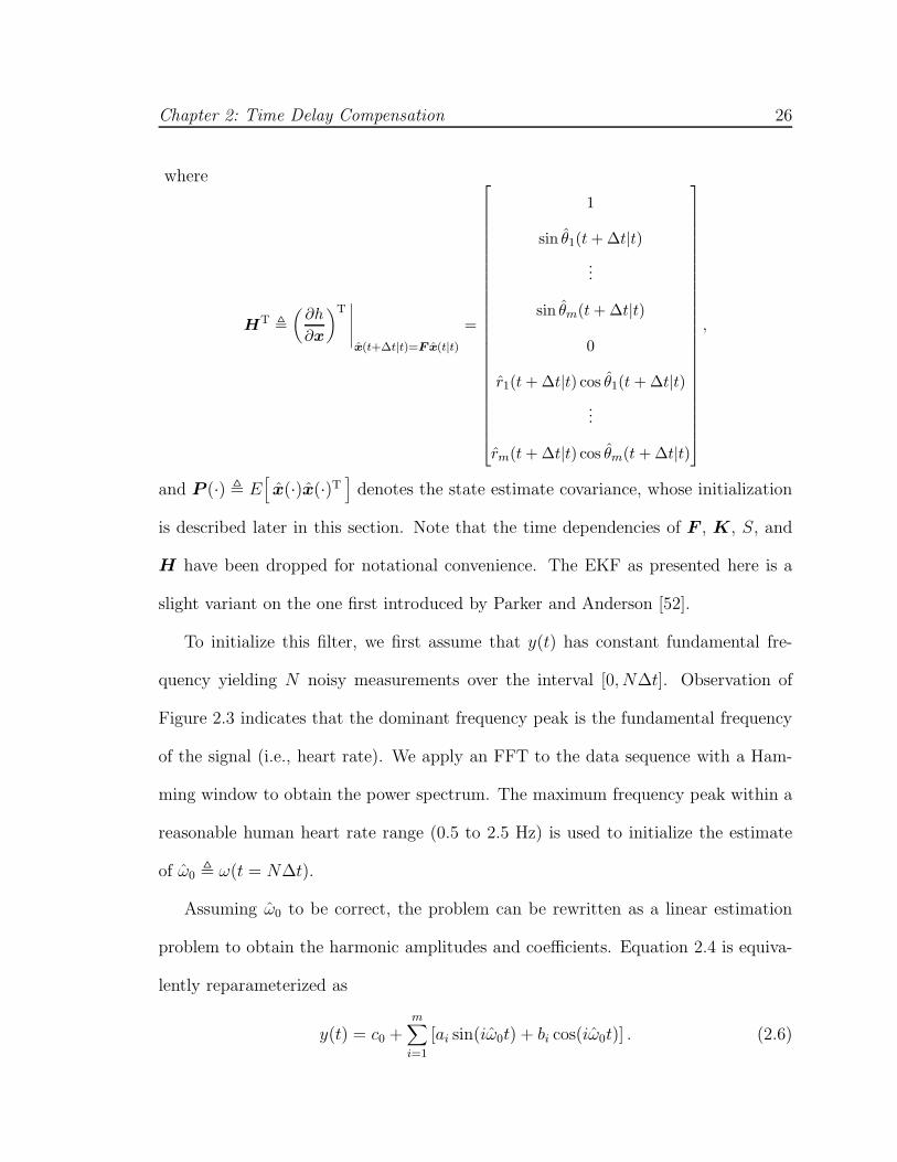
Chapter 2: Time Delay Compensation 26
where
HT ,
(
∂h
∂x
)T∣
∣
∣
∣
∣
x(t+∆t|t)=Fx(t|t)
=
1
sin θ1(t + ∆t|t)...
sin θm(t + ∆t|t)
0
r1(t + ∆t|t) cos θ1(t + ∆t|t)...
rm(t + ∆t|t) cos θm(t + ∆t|t)
,
and P (·) , E[
x(·)x(·)T]
denotes the state estimate covariance, whose initialization
is described later in this section. Note that the time dependencies of F , K, S, and
H have been dropped for notational convenience. The EKF as presented here is a
slight variant on the one first introduced by Parker and Anderson [52].
To initialize this filter, we first assume that y(t) has constant fundamental fre-
quency yielding N noisy measurements over the interval [0, N∆t]. Observation of
Figure 2.3 indicates that the dominant frequency peak is the fundamental frequency
of the signal (i.e., heart rate). We apply an FFT to the data sequence with a Ham-
ming window to obtain the power spectrum. The maximum frequency peak within a
reasonable human heart rate range (0.5 to 2.5 Hz) is used to initialize the estimate
of ω0 , ω(t = N∆t).
Assuming ω0 to be correct, the problem can be rewritten as a linear estimation
problem to obtain the harmonic amplitudes and coefficients. Equation 2.4 is equiva-
lently reparameterized as
y(t) = c0 +m∑
i=1
[ai sin(iω0t) + bi cos(iω0t)] . (2.6)
Chapter 2: Time Delay Compensation 27
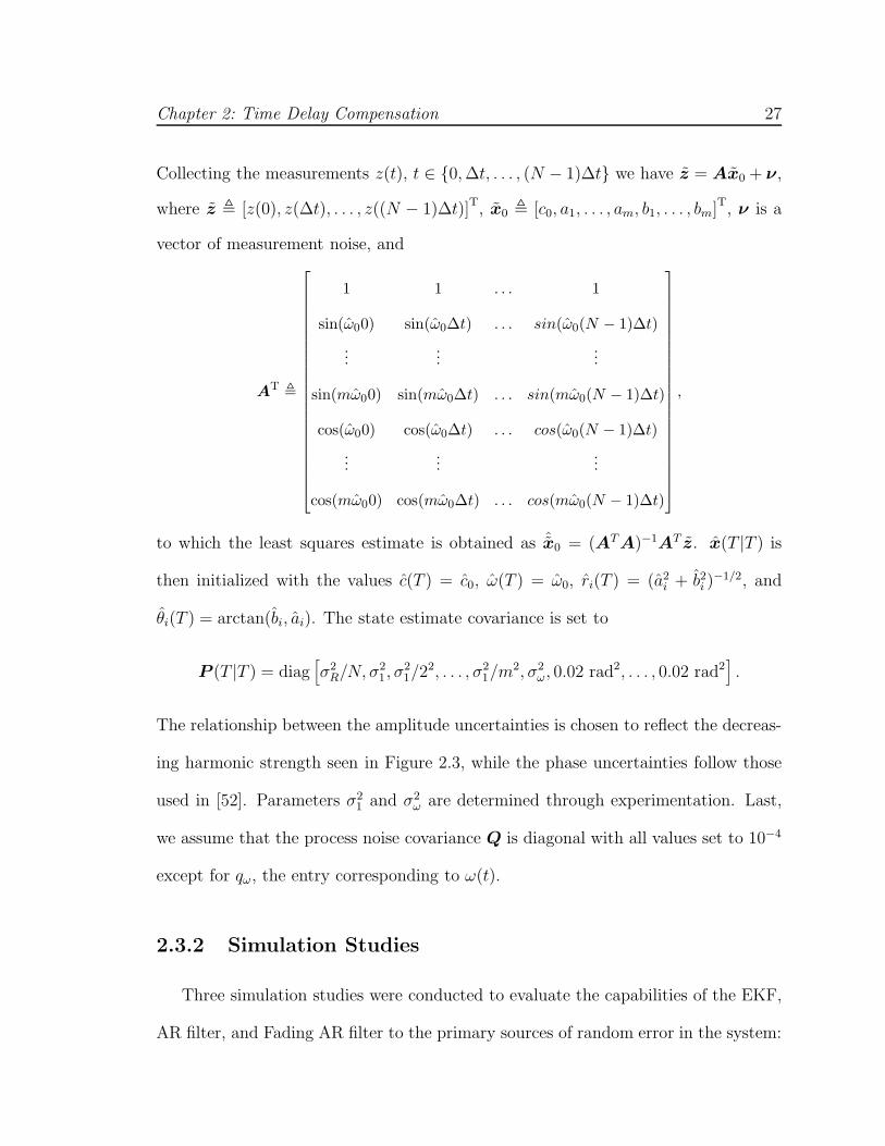
Collecting the measurements z(t), t ∈ {0, ∆t, . . . , (N − 1)∆t} we have z = Ax0 + ν,
where z , [z(0), z(∆t), . . . , z((N − 1)∆t)]T, x0 , [c0, a1, . . . , am, b1, . . . , bm]T, ν is a
vector of measurement noise, and
AT ,
1 1 . . . 1
sin(ω00) sin(ω0∆t) . . . sin(ω0(N − 1)∆t)
......
...
sin(mω00) sin(mω0∆t) . . . sin(mω0(N − 1)∆t)
cos(ω00) cos(ω0∆t) . . . cos(ω0(N − 1)∆t)
......
...
cos(mω00) cos(mω0∆t) . . . cos(mω0(N − 1)∆t)
,
to which the least squares estimate is obtained as ˆx0 = (AT A)−1AT z. x(T |T ) is
then initialized with the values c(T ) = c0, ω(T ) = ω0, ri(T ) = (a2i + b2
i )−1/2, and
θi(T ) = arctan(bi, ai). The state estimate covariance is set to
P (T |T ) = diag[
σ2R/N, σ2
1, σ21/22, . . . , σ2
1/m2, σ2
ω, 0.02 rad2, . . . , 0.02 rad2]
.
The relationship between the amplitude uncertainties is chosen to reflect the decreas-
ing harmonic strength seen in Figure 2.3, while the phase uncertainties follow those
used in [52]. Parameters σ21 and σ2
ω are determined through experimentation. Last,
we assume that the process noise covariance Q is diagonal with all values set to 10−4
except for qω, the entry corresponding to ω(t).
2.3.2 Simulation Studies
Three simulation studies were conducted to evaluate the capabilities of the EKF,
AR filter, and Fading AR filter to the primary sources of random error in the system:

Chapter 2: Time Delay Compensation 28
0.5 1 1.5 2 2.5 3
0.5
1
1.5
2
2.5
3
σR (mm)
Pre
dic
tion E
rror
(mm
)Last Cycle
WFLC
AR
Fading AR
EKF
A
−10 −8 −6 −4 −2 0 2 4 6 8 10
0.5
1
1.5
2
2.5
3
3.5
4
4.5
5
∆ HR (bpm)
Pre
dic
tion E
rror
(mm
)
Last Cycle
WFLC
AR
Fading AR
B
Figure 2.8: RMS prediction error results for parametric simulation studies. A: Errorfor varying measurement noise; B: Error for step heart rate changes.
measurement noise and heart rate variability. For illustrative purposes, the filters
were also compared to the WFLC estimator [53] and a simpler method of using the
previous cardiac cycle trajectory for the prediction of the next. A more sophisticated
version of the latter method, termed Last Cycle here, was used successfully in a
beating heart tracking system [6].
In the first simulation, we subjected the predictors to varying levels of measure-
ment noise on a fixed-rate trajectory (60 bpm). The mitral valve annulus trajectory of
Figure 2.2 was reinterpolated to 28 Hz and corrupted by additive zero-mean Gaussian
noise with standard deviation 0.3 ≤ σR ≤ 3 mm. Each predictor was then given 30 s
of data to initialize and performance was judged for the following 10 s on 1-sample
ahead predictions.
The RMS errors for each predictor averaged across 100 monte-carlo trials are
shown in Figure 2.8A. The EKF, WFLC, AR, and Fading AR filtering methods clearly
give higher accuracy predictions than the inherent uncertainty of the measurements,
with the EKF doing the best. As expected, the Last Cycle method had error statistics
equal to σR since it attempts no smoothing. It should be noted that the Fading AR

Chapter 2: Time Delay Compensation 29
filter was tuned with f = 0.985 in order to achieve errors that are approximately equal
to σR. This setting represents the lowest reasonable value for the Fading AR filter
since a value lower would give performance below the Last Cycle method. The EKF
was run with m = 8 harmonics, N = 280 initialization points (10 s), σ21 = 2 mm2,
σ2ω = 0.11 (rad/sec)2 (roughly twice the frequency resolution of the FFT), and qω =
10−3 (rad/sec)2. The WFLC was initialized in the same manner as the EKF, run
with m = 8 harmonics, and experimentally set with its adaptive gain parameters
µ0 = 7×10⁻⁶ and µ1 = 0.03 for best performance in this and subsequent simulations.
In a second parametric simulation study, we gauged the tolerance of each predictor
to a sudden change in heart rate. A trajectory was assembled by piecing together 30 s
of heart motion at 60 bpm and 10 s of motion at (60+∆HR) bpm. The second portion
of the trajectory was generated by compression/dilation of the target trajectory in
Figure 2.2 to obtain the desired heart rate. Like before, the composite trajectory
was reinterpolated to 28 Hz and corrupted with additive, Gaussian, zero-mean noise
with σR = 1.30 mm. The last 10 s were used to evaluate performance. A reasonable
range of −10 bpm ≤ ∆HR ≤ 10 bpm was determined from clinical heart rate data
(Figure 2.9), which is discussed in more detail later in this section.
Figure 2.8B shows the mean RMS errors for each predictor across 100 monte-
carlo trials. The EKF provided better predictions than the other four methods. It
was also the only method that yielded sub-σR error for the majority of heart rate
changes. The WFLC had similar accuracies to the EKF at small ∆HR but showed
slow convergence to the new heart rate for ∆HR > 4 bpm. As expected, the accuracy
of the AR filter also approached that of the EKF for small ∆HR and quickly degraded

Chapter 2: Time Delay Compensation 30
as ∆HR increased. Exponential weighting of the measurements allowed the filter to
adjust to changes in the trajectory, as demonstrated by the Fading AR filter’s superior
performance over the AR filter for large ∆HR. However, this adaptability lessened
accuracy when the trajectory did not change significantly. Finally, the Last Cycle
method showed performance comparable to the Fading AR filter. For this simulation
all filter parameters were chosen the same as in the previous simulation, with the
exception of qω = 5 × 10⁻³ (rad/s)2 and σ2ω = 1 (rad/s)2 for the EKF.
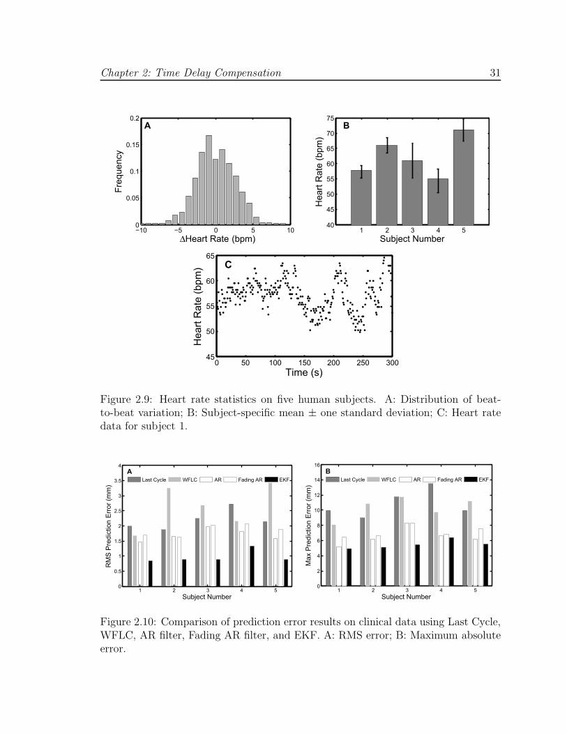
Finally, to investigate the performance of each predictor to the more realistic case
of a continuously changing heart rate, we modulated the period of the annulus trajec-
tory with clinically-obtained cardiac cycle records. Annotated ECG records for five
human subjects were selected from the MIT-BIH Normal Sinus Rhythm Database [25]
and composite mitral valve annulus trajectories were generated in a manner similar
to the previous simulation study. Noise-corrupted measurements were generated as
before, with σR = 1.30 mm. Summary statistics for each subject are presented in
Figure 2.9B and an example of the beat-to-beat heart rate for subject number 1 is
shown in Figure 2.9C.
Results from this study indicate that the EKF is more suited to tracking and
prediction in this application than the other four methods because it adjusts to rapid
changes in heart rate through explicit modeling of quasiperiodicity (Figure 2.10).
Interestingly, the AR filter showed moderately better performance than the Fading
AR filter. The reason for this is that the AR filter locked on to an “average” trajectory
for each subject while the Fading AR filter continuously readjusted to more recent
noisy data. Ultimately, deviations from the “average” motion were less than the
Chapter 2: Time Delay Compensation 31
−10 −5 0 5 100
0.05
0.1
0.15
0.2
∆Heart Rate (bpm)
Fre
quency
A
1 2 3 4 540
45
50
55
60
65
70
75
Subject Number
Heart
Rate
(bpm
)
B
0 50 100 150 200 250 30045
50
55
60
65
Time (s)
Heart
Rate
(bpm
) C
Figure 2.9: Heart rate statistics on five human subjects. A: Distribution of beat-to-beat variation; B: Subject-specific mean ± one standard deviation; C: Heart ratedata for subject 1.
1 2 3 4 50
0.5
1
1.5
2
2.5
3
3.5
4
Subject Number
RM
S P
redic
tion E
rror
(mm
)
Last Cycle WFLC AR Fading AR EKF
A
1 2 3 4 50
2
4
6
8
10
12
14
16
Subject Number
Max P
redic
tion E
rror
(mm
)
Last Cycle WFLC AR Fading AR EKF
B
Figure 2.10: Comparison of prediction error results on clinical data using Last Cycle,WFLC, AR filter, Fading AR filter, and EKF. A: RMS error; B: Maximum absoluteerror.
Chapter 2: Time Delay Compensation 32
measurement noise. The Last Cycle method performed worse for similar reasons:
persistent variations in heart rate and measurement noise degraded the accuracy of
the previous cycle as a predictor for the next. The slow convergence of the WFLC to
changing heart rates caused it to have severely degraded performance.
2.4 Performance Evaluation in a Surgical Task
In order to quantify the amount of assistance that motion compensation provides
to operators working on a moving target, we conducted two studies of user perfor-
mance with the MCI in an in vitro setting. These studies additionally provide insight
on how sensitive performance is to the shortcomings of a 3D ultrasound-guided sys-
tem. Specifically, User Study 1 determined the extent to which user performance is
dependent on time delay and random positional error. User Study 2 investigated user
performance with EKF delay compensation on targets with both fixed and variable
heart rates. Subjects performed a drawing task on a moving target using the MCI
under different tracking conditions. A total of eighteen test subjects (fourteen male
and four female, aged 22 to 36; eight subjects for User Study 1 and ten subjects for
User Study 2) voluntarily participated following informed consent under a protocol
approved by the University Institutional Review Board.
2.4.1 Experimental Setup
The tests were run on a setup that emulates the intended surgical environment.
To simulate the moving mitral valve, a target platform was mounted on a cam-driven
device that replicates the 1D motion of the mitral valve annulus centroid as measured
Chapter 2: Time Delay Compensation 33
from the 3D ultrasound tracking data. During trials, a paper target was affixed to this
platform to record the subject’s drawing. A 0.5 cm hard foam rubber pad between
the target paper and target platform provided a small measure of compliance. In
combination with the pen used in the trials, the pad had a stiffness of 4.5 N/mm.
For the purposes of this experiment, the cam was used to simulate a heart rate of
60 bpm. Opposite the target platform, the MCI was mounted in a gimbal allowing
both angular motion and translation towards and away from the target (Figure 2.11).
A rod was mounted on the MCI with a ballpoint pen affixed to one end and a force
sensor incorporated along its length. The force sensor had a stiffness of 10 N/mm.
In place of the 3D ultrasound-based tracking and controls algorithms that would be
used in surgery, target position was directly measured at 1 kHz by a contact arm with
a potentiometer attached to the target platform. This sensing method provided the
robust tracking data necessary to evaluate the efficacy of MCI mitral valve annulus
tracking and the performance of predictive filtering algorithms.
2.4.2 User Task
Subjects were instructed to draw a circle on the moving target platform. The
circle had to be drawn between two concentric target circles with 2.29 cm and 2.92 cm
diameters. Subjects started at the top of the circle and proceeded in the clockwise
direction. If the pen bounced off of the target surface or outside of the target circles,
the subject was instructed to continue drawing from the clockwise-most mark that
they made between the target circles. Subjects could only draw around the circle
once. They could not go back to draw in gaps that they originally missed. To
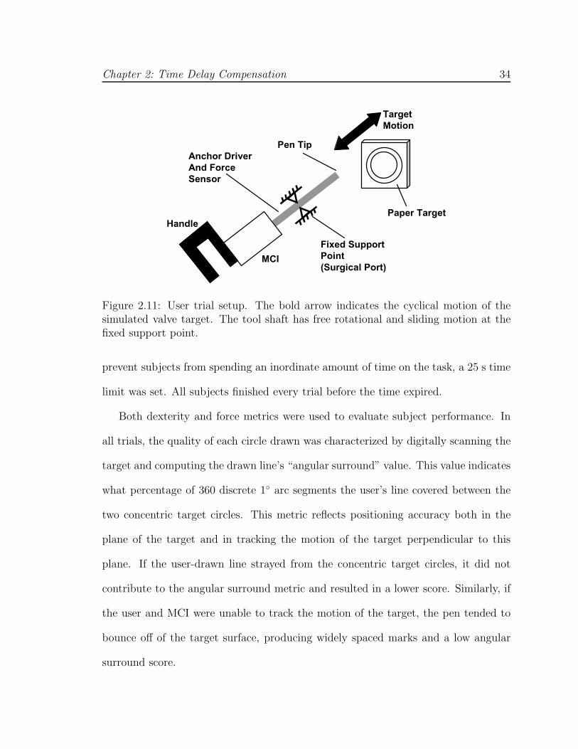
Chapter 2: Time Delay Compensation 34
MCI
Handle
Fixed Support
Point
(Surgical Port)
Pen Tip
Anchor Driver
And Force
Sensor
Paper Target
Target
Motion
Figure 2.11: User trial setup. The bold arrow indicates the cyclical motion of thesimulated valve target. The tool shaft has free rotational and sliding motion at thefixed support point.
prevent subjects from spending an inordinate amount of time on the task, a 25 s time
limit was set. All subjects finished every trial before the time expired.
Both dexterity and force metrics were used to evaluate subject performance. In
all trials, the quality of each circle drawn was characterized by digitally scanning the
target and computing the drawn line’s “angular surround” value. This value indicates
what percentage of 360 discrete 1◦ arc segments the user’s line covered between the
two concentric target circles. This metric reflects positioning accuracy both in the
plane of the target and in tracking the motion of the target perpendicular to this
plane. If the user-drawn line strayed from the concentric target circles, it did not
contribute to the angular surround metric and resulted in a lower score. Similarly, if
the user and MCI were unable to track the motion of the target, the pen tended to
bounce off of the target surface, producing widely spaced marks and a low angular
surround score.

Chapter 2: Time Delay Compensation 35
The axial force applied by the subject to the target was also recorded for four of
the eight test subjects in User Study 1 and nine of the ten subjects in User Study 2.
In all eighteen cases, subjects were informed of both evaluation metrics. They were
instructed that their foremost objective was to draw continuous circles conforming to
the angular surround metric and only secondly to use the minimum amount of force
necessary.
This task was selected to emulate the motion requirements of placing a surgical
anchor. In order to apply the surgical anchors developed for this procedure, the tip
of the anchor driver, consisting of 14 gauge hypodermic tubing, must be accurately
located and pressed against the target surface with a force of at least 1.5 N [68]. This
contact must be maintained for several seconds as the surgeon inserts the anchor,
tests whether it is properly deployed, and then releases the anchor. This process
requires a combination of accuracy and prolonged contact with the surface. At the
same time, forces must be minimized so as not to cause damage to the valve.
2.4.3 Independent Variables
User Study 1: Tracking with Time Delay and Positional Error
Subjects of User Study 1 completed the task in eight different tracking conditions.
In the “solid” condition, the motion of the MCI was rigidly locked in order to simulate
a traditional, solid endoscopic tool. For the “baseline” MCI tracking condition, the
current position of the target (0.015 mm RMS error) was sent to the MCI as a
position command. This baseline condition resulted in a 14 ms delay. The remaining
six tracking conditions were divided into two groups of three conditions corresponding

Chapter 2: Time Delay Compensation 36
to differing levels of the considered error.
Random positional error was simulated by the superposition of a time-varying
error value with the cam position command used in the baseline tracking state. A
new positional error was calculated at 8 Hz. These errors were uniformly distributed
random values ([−1, 1]), multiplied by an amplitude factor of 0.35 mm, 0.70 mm, or
1.05 mm.
Delay error was implemented by recording the cam tracking position and holding
it for a specified period before sending this position to the MCI as a motion command.
For this set of trials, the three levels of added delay used were 25 ms, 35 ms, and
45 ms. Including the MCI lag time of 14 ms, the effective delay settings were 39 ms,
49 ms, and 59 ms. This range of times was chosen as representative of the imaging and
transmission delays associated with real-time 3D ultrasound-guided procedures [48].
User Study 2: Delay-Compensated Tracking with Heart Rate Variation
and Measurement Noise
To test the EKF under conditions similar to those seen in 3D ultrasound-guided
procedures, the 1 kHz measurements of target position were downsampled to 28 Hz
and corrupted by additive, zero-mean Gaussian noise with variance 1.302 [46]. The
target was commanded to beat at 60 bpm or with a variable rate that had additive,
zero-mean Gaussian beat-to-beat fluctuations with variance σ2HR. Finally, a time
delay of 39 ms, 59 ms, or 89 ms was injected into the measurements to simulate the
delays encountered with 3D ultrasound. Note that the 89 ms delay exceeds the delays
used in User Study 1 to also account for the additional computational delays from
Chapter 2: Time Delay Compensation 37
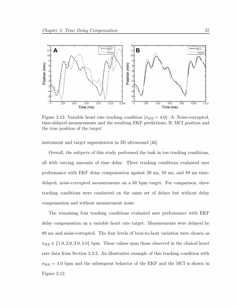
A B
Figure 2.12: Variable heart rate tracking condition (σHR = 4.0). A: Noise-corrupted,time-delayed measurements and the resulting EKF predictions; B: MCI position andthe true position of the target.
instrument and target segmentation in 3D ultrasound [46].
Overall, the subjects of this study performed the task in ten tracking conditions,
all with varying amounts of time delay. Three tracking conditions evaluated user
performance with EKF delay compensation against 39 ms, 59 ms, and 89 ms time-
delayed, noise-corrupted measurements on a 60 bpm target. For comparison, three
tracking conditions were conducted on the same set of delays but without delay
compensation and without measurement noise.
The remaining four tracking conditions evaluated user performance with EKF
delay compensation on a variable heart rate target. Measurements were delayed by
89 ms and noise-corrupted. The four levels of beat-to-beat variation were chosen as
σHR ∈ {1.0, 2.0, 3.0, 4.0} bpm. These values span those observed in the clinical heart
rate data from Section 2.3.2. An illustrative example of this tracking condition with
σHR = 4.0 bpm and the subsequent behavior of the EKF and the MCI is shown in
Figure 2.12.
Chapter 2: Time Delay Compensation 38
2.4.4 Testing Protocol
Each subject test consisted of a practice period followed by the trials corresponding
to the tracking conditions of their study. Practice was intended to familiarize the test
subject with the MCI and the evaluation task in order to bring subjects to a uniform
level of ability and to limit learning effects during trials. Practice was divided into
three one-minute segments during which the subject was free to experiment with
using the MCI to draw on a target paper. During the first minute of training, the
target was stationary and the tool was set in the solid condition. The second minute
of training involved a moving target and a solid tool. In the third and final minute,
the target was moving and the MCI was in the baseline tracking condition. Following
the completion of training, each test subject ran through the trials corresponding
to the tracking conditions of their study. The order in which these conditions were
administered was varied between trials using a balanced Latin square to minimize the
effects of between-trial carry-over and learning on collected data.
The means of collected angular surround error metric were compared for sta-
tistically significant differences using the SPSS statistical analysis software package
(Version 14.0, SPSS Inc., Chicago, IL, USA). These comparisons were made using
t-tests and ANOVA with an LSD post hoc test. In all cases, significance corresponds
to p < 0.05.
Chapter 2: Time Delay Compensation 39
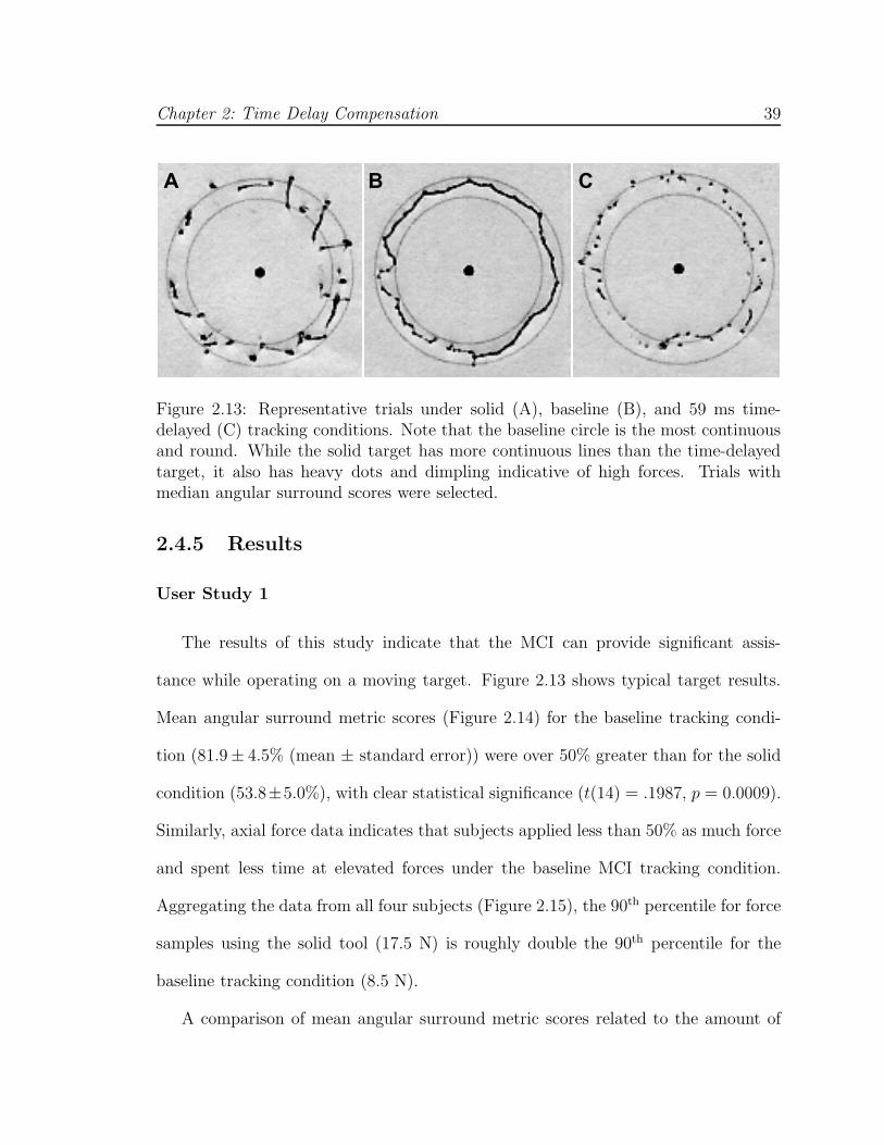
A B C
Figure 2.13: Representative trials under solid (A), baseline (B), and 59 ms time-delayed (C) tracking conditions. Note that the baseline circle is the most continuousand round. While the solid target has more continuous lines than the time-delayedtarget, it also has heavy dots and dimpling indicative of high forces. Trials withmedian angular surround scores were selected.
2.4.5 Results
User Study 1
The results of this study indicate that the MCI can provide significant assis-
tance while operating on a moving target. Figure 2.13 shows typical target results.
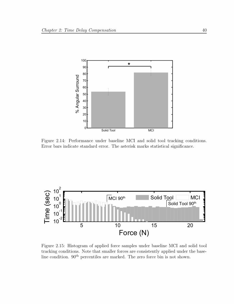
Mean angular surround metric scores (Figure 2.14) for the baseline tracking condi-
tion (81.9± 4.5% (mean ± standard error)) were over 50% greater than for the solid
condition (53.8±5.0%), with clear statistical significance (t(14) = .1987, p = 0.0009).
Similarly, axial force data indicates that subjects applied less than 50% as much force
and spent less time at elevated forces under the baseline MCI tracking condition.
Aggregating the data from all four subjects (Figure 2.15), the 90th percentile for force
samples using the solid tool (17.5 N) is roughly double the 90th percentile for the
baseline tracking condition (8.5 N).
A comparison of mean angular surround metric scores related to the amount of
Chapter 2: Time Delay Compensation 40
Solid Tool MCI0
10
20
30
40
50
60
70
80
90
100
% A
ngula
r S
urr
ound
*
Figure 2.14: Performance under baseline MCI and solid tool tracking conditions.Error bars indicate standard error. The asterisk marks statistical significance.
5 10 15 2010
-210
-110
010
110
2
Force (N)
Tim
e (
sec)
Solid Tool MCIMCI 90th
Solid Tool 90th
Figure 2.15: Histogram of applied force samples under baseline MCI and solid tooltracking conditions. Note that smaller forces are consistently applied under the base-line condition. 90th percentiles are marked. The zero force bin is not shown.

Chapter 2: Time Delay Compensation 41
14 39 49 590
10
20
30
40
50
60
70
80
90
100
% A
ngula
r S
urr
ound
Tracking Delay (ms)
*
*
Figure 2.16: Performance under de-lay tracking conditions. Error bars in-dicate standard error. Asterisks in-dicate statistical significance. Dottedline shows fitted linear model (R2 =0.9937).
0 0.35 0.7 1.050
10
20
30
40
50
60
70
80
90
100
% A
ngula
r S
urr
ound
Amplitude of Random Error (mm)
Figure 2.17: Performance under posi-tional error tracking conditions. Errorbars indicate standard error.
delay error (Figure 2.16) demonstrates decreases in performance ranging from 67%
to 33% with increasing delay (f(3, 28) = 16.005, p < .001). Statistically significant
differences were indicated between the baseline condition and tracking with delays of
39 ms (61.2 ± 1.5%), 49 ms (56.0 ± 3.7%), and 59 ms (48.8 ± 3.8%). A significant
difference also exists between the means of the 39 ms and 59 ms tracking conditions
(p = 0.02). Trend analysis indicates that the data is well fit by a linear model
(p < 0.001).
An analysis of mean angular surround metric scores related to positional error
did not demonstrate significant differences under ANOVA analysis (f(3, 28) = 0.638,
p = 0.597). As seen in Figure 2.17, the mean score under the baseline condition
differed very little from those with error amplitude factors of 0.35 mm (81.7± 3.3%),
0.70 mm (78.0 ± 5.5%), and 1.05 mm (74.2 ± 4.6%).

Chapter 2: Time Delay Compensation 42
User Study 2
Results from this study demonstrate that the EKF is an effective approach for
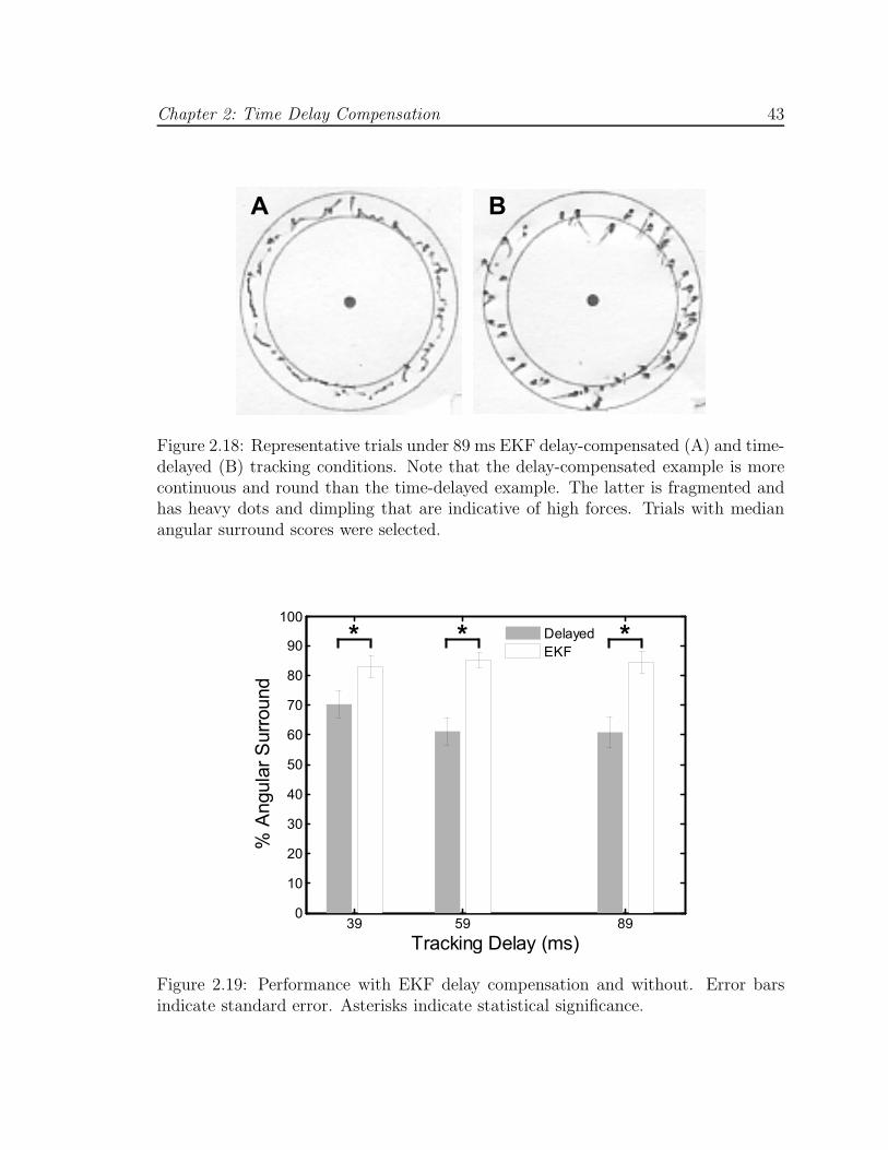
compensating time delay. Figure 2.18 shows typical target results. Mean angular
surround scores for EKF delay-compensated tracking (Figure 2.19) were similar to
the baseline tracking condition from User Study 1 for all three conditions of 39 ms
(83.1 ± 3.7%), 59 ms (85.2 ± 2.6%), and 89 ms (84.4 ± 3.8%). Likewise, delay-
compensated tracking showed performance increases over delayed tracking ranging
from 13% to 24%. The mean angular scores for delayed tracking were 70.4 ± 4.8%,
61.1 ± 4.6%, and 61.0± 5.2% for 39, 59, and 89 ms delays, respectively. Statistically
significant differences at p < 0.05 were observed between the mean scores of each
delay-compensated tracking condition to each delayed tracking condition. Delay-
compensated tracking also yielded smaller axial forces than those observed for delayed
tracking (Figure 2.20).
An analysis of mean angular surround metric scores related to heart rate variability
did not demonstrate significant differences under ANOVA analysis (f(3, 36) = 0.705,
p = 0.555). As seen in Figure 2.21, the performance against a fixed-rate target was
comparable to that against a variable rate target with σHR equal to 1.0 bpm (85.9±
2.6%), 2.0 bpm (84.1 ± 2.9%), 3.0 bpm (80.5 ± 3.6%), and 4.0 bpm (81.5 ± 2.5%).
Chapter 2: Time Delay Compensation 43
A B
Figure 2.18: Representative trials under 89 ms EKF delay-compensated (A) and time-delayed (B) tracking conditions. Note that the delay-compensated example is morecontinuous and round than the time-delayed example. The latter is fragmented andhas heavy dots and dimpling that are indicative of high forces. Trials with medianangular surround scores were selected.
39 59 890
10
20
30
40
50
60
70
80
90
100
% A
ngula
r S
urr
ound
Tracking Delay (ms)
Delayed
EKF* * *
Figure 2.19: Performance with EKF delay compensation and without. Error barsindicate standard error. Asterisks indicate statistical significance.

Chapter 2: Time Delay Compensation 44
5 10 15 2010
-2
10-1
100
101
Tim
e (
s)
Delayed
EKF
5 10 15 2010
-2
10-1
100
101
Tim
e (
s)
5 10 15 2010
-2
10-1
100
101
Tim
e (
s)
Force (N)
A
B
C
Figure 2.20: Force application with and without delay compensation for delays of39 ms (A), 59 ms (B), and 89 ms (C). Note that smaller forces are consistentlyapplied under the delay-compensated tracking conditions. The zero force bin is notshown.
0 1 2 3 40
10
20
30
40
50
60
70
80
90
100
% A
ngul
ar S
urro
und
sHR
(bpm)
Figure 2.21: Performance under variable heart rate tracking conditions. Error barsindicate standard error.

Chapter 2: Time Delay Compensation 45
2.5 System Accuracy Under 3D Ultrasound
Guidance
Water tank experiments were conducted to measure the motion synchronization
accuracy of the system under 3D ultrasound guidance. To do these, a real-time 3D
ultrasound target segmentation algorithm was first incorporated into the system to
provide position measurements to the EKF. The target was set to be an X-shaped
fiducial that can be easily mounted to an annuloplasty ring (Figure 2.22B). This
fiducial was specifically chosen because detecting two intersecting lines is suited for an
existing real-time 3D ultrasound segmentation algorithm based on the modified Radon
transform [46]. This algorithm is known to provide target position measurements with
1.30 mm RMS accuracy under in vitro conditions. Because higher noise is present
in vivo, we also tested this system in two other noise conditions in which large, zero
mean Gaussian terms with standard deviations of 2.0 mm or 3.0 mm were added to
the segmented target positions. This yielded three noise conditions with overall RMS
accuracies of σR ∈ {1.30, 3.30, 4.30} mm.
2.5.1 Experimental Setup
The target and instrument were imaged by a real-time 3D ultrasound probe in a
water tank at 28 Hz (Figure 2.22A). Data was streamed from the ultrasound machine
(SONOS 7500, Philips Healthcare, Andover, MA) to a computer over an ethernet
connection. The stream was captured by the computer and passed to a graphics pro-
cessing unit (8800GTS, nVidia Corp, Santa Clara, CA) where the volumes were auto-

Chapter 2: Time Delay Compensation 46
MCI
Handle
Fiducial
Target
Target
Motion
Water Tank
3DUS
Probe
3DUS
Volume
Anchor Driver
A B
Figure 2.22: Setup for motion synchronization experiments (A) and X-shaped fiducialtarget (B).
matically segmented using the modified Radon transform segmentation algorithm [46]
to obtain target position measurements. The measurements were corrupted with ad-
ditive Gaussian noise (depending on the noise condition), then passed to a third
thread for EKF processing. This returned predicted target positions 82 ms in the
future (68 ms from imaging and segmentation, 14 ms from instrument lag time) and
were sent to the 1 kHz PID control loop for the robot.
Five motion synchronization trials were conducted per noise condition. The target
simulated mitral valve motion at 60 bpm with the cam-driven mechanism described
in Section 2.4.1. MCI position and true target position were measured at 1 kHz with
potentiometers and stored for offline processing. Target measurements and EKF
predictions were acquired at the 3D ultrasound sampling rate (28 Hz) and stored as
well. Accuracy evaluation was done on the 20 s of tracking data following 20 s of
EKF initialization.

Chapter 2: Time Delay Compensation 47
2.5.2 Results
Typical data and results for each noise condition are shown in Figure 2.23 and
overall performance is summarized in Figure 2.24. Mean RMS accuracies for EKF
predictions were 1.01 ± 0.02 mm, 1.08 ± 0.03 mm, and 1.22 ± 0.05 mm for noise
levels of 1.30 mm, 3.30 mm, and 4.30 mm (respectively) and showed statistically
significant reductions in measurement error (p < 0.0001 for each case). Mean MCI
synchronization errors were 1.15±0.04 mm, 1.23±0.06 mm, and 1.28±0.10 mm RMS
for the three noise conditions. The mean RMS error added to the system from the
MCI following the prescribed EKF trajectory was 0.14± 0.01 mm and this difference
was statistically significant (p = 0.002). The RMS noise accuracy for the X-tracking
algorithm observed across all 15 trials was 1.30±0.01 mm, in agreement with previous
reports [46].
2.6 Discussion
In vitro user trials demonstrate that a motion compensation system is an effective
aid for surgical tasks on the beating mitral valve annulus. Motion synchronization
allowed users to operate with both increased dexterity and reduced forces. In User
Study 1, the angular surround scores indicative of dexterity increased by approxi-
mately 50% between the solid tool and baseline tracking conditions while the 90th
percentile for force decreased by a similar ratio. These performance gains were main-
tained when increasing levels of positional error were inserted into the system, but
disappeared when uncompensated time delays were added to the tracking data.

Chapter 2: Time Delay Compensation 48
25 25.5 26 26.5 27
−10
−5
0
5
10
Time (s)
Position (mm) A Meas EKF
25 25.5 26 26.5 27
−10
−5
0
5
10
Time (s)
Position (mm) B Target MCI
25 25.5 26 26.5 27
−10
−5
0
5
10
Time (s)
Position (mm) C Meas EKF
25 25.5 26 26.5 27
−10
−5
0
5
10
Time (s)
Position (mm) D Target MCI
25 25.5 26 26.5 27
−10
−5
0
5
10
Time (s)
Position (mm) E Meas EKF
25 25.5 26 26.5 27
−10
−5
0
5
10
Time (s)
Position (mm) F Target MCI
Figure 2.23: Examples of data, filtering, and motion tracking results. Left columnshows measurements from 3D ultrasound target segmentation and EKF predictedtarget trajectories for each noise condition (σR = 1.30 mm (A), 3.30 mm (C), and4.30 mm (E)). Corresponding MCI and true target trajectories for each noise condition(σR = 1.30 mm (B), 3.30 mm (D), 4.30 mm (F)) are shown in the right column.
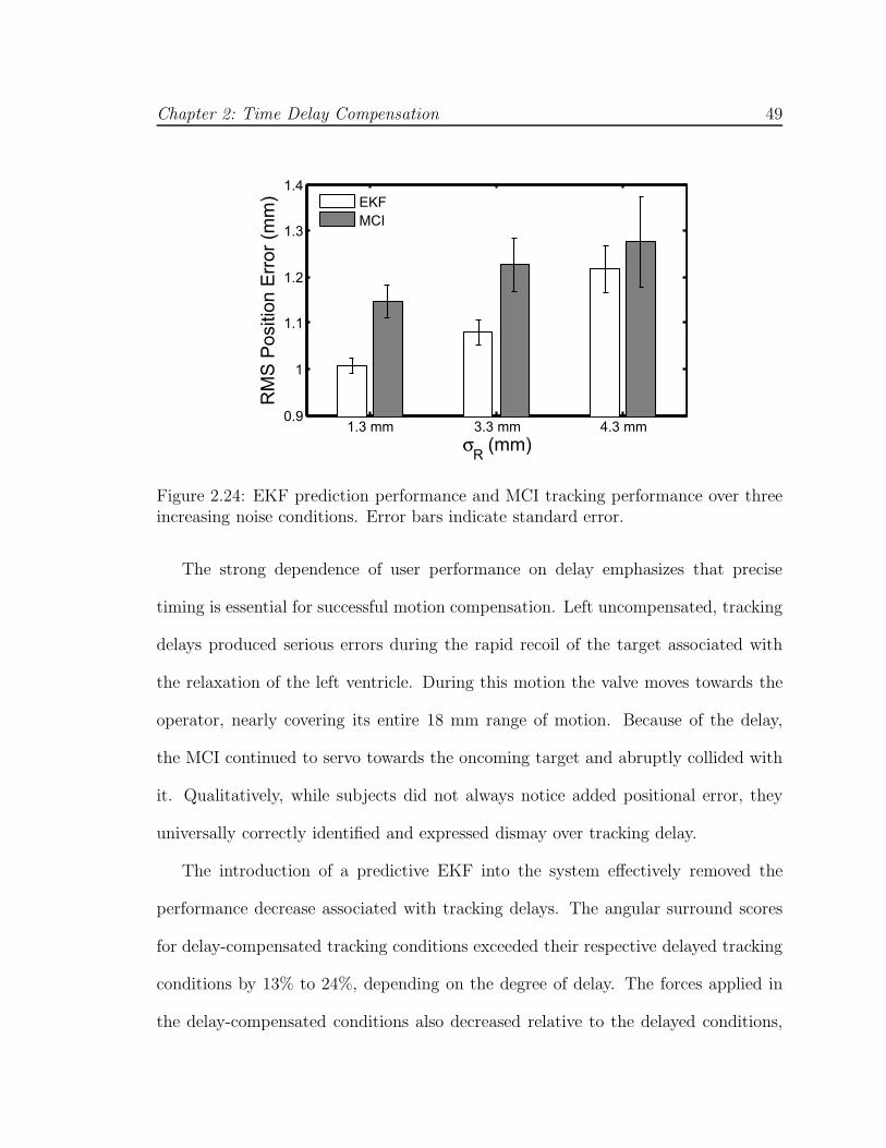
Chapter 2: Time Delay Compensation 49
1.3 mm 3.3 mm 4.3 mm0.9
1
1.1
1.2
1.3
1.4
σR (mm)
RM
S P
ositio
n E
rror
(mm
) EKF
MCI
Figure 2.24: EKF prediction performance and MCI tracking performance over threeincreasing noise conditions. Error bars indicate standard error.
The strong dependence of user performance on delay emphasizes that precise
timing is essential for successful motion compensation. Left uncompensated, tracking
delays produced serious errors during the rapid recoil of the target associated with
the relaxation of the left ventricle. During this motion the valve moves towards the
operator, nearly covering its entire 18 mm range of motion. Because of the delay,
the MCI continued to servo towards the oncoming target and abruptly collided with
it. Qualitatively, while subjects did not always notice added positional error, they
universally correctly identified and expressed dismay over tracking delay.
The introduction of a predictive EKF into the system effectively removed the
performance decrease associated with tracking delays. The angular surround scores
for delay-compensated tracking conditions exceeded their respective delayed tracking
conditions by 13% to 24%, depending on the degree of delay. The forces applied in
the delay-compensated conditions also decreased relative to the delayed conditions,

Chapter 2: Time Delay Compensation 50
although to a lesser extent than seen between baseline tracking and the solid tool. The
delay-compensated scores of User Study 2 marginally exceeded the baseline scores of
User Study 1 by an amount that is consistent with the removal of the MCI’s 14 ms lag
time (as predicted by the linear model from User Study 1). However, caution must
be taken when making a direct comparison of the angular surround scores between
User Studies 1 and 2 because of differing amounts of in-trial training (eight trials
in User Study 1 and ten trials in User Study 2). It is reasonable to conclude that
EKF delay compensation restored the MCI tracking performance to at least baseline
tracking conditions in cases of delay. Moreover, the performance increases observed
for delay-compensated tracking showed no degradation across the range of time delays
expected for 3D ultrasound-guided procedures.
The levels of random positional error explored in the user studies had a negligible
effect on the benefits of MCI tracking. No statistically significant differences were
found between user performance under all three positional error conditions and the
baseline condition. This result suggests that if the timing with the valve’s sudden
recoil is maintained, the value of the MCI’s tracking is robust in the face of positional
errors as high as ±1 mm. This may be attributed, in part, to compliance in the
system: in the MCI’s mechanism and in the foam pad on the target platform, which
introduce compliance similar in nature to that in the heart.
Heart rate variations in the target motion also provided no significant degradation
in user performance over the clinically-obtained beat-to-beat statistics (Figure 2.9).
This is not surprising given that the EKF estimates did not degrade on these levels
of heart rate variation. In some respects, tracking a variable rate target was another
Chapter 2: Time Delay Compensation 51
approach to injecting positional error into the system since the filter remained in
phase with the target (see, for instance, Figure 2.12). Extremely large beat-to-beat
variations would cause the EKF to break synchronization with the target because
the linearization of the measurement function h(x(t)) would become inappropriate.
There are several potential routes for improvement if more aggressive heart rate vari-
ations than those explored here are encountered. First, heart rate variability could
be reduced through drug treatment and electrical pacing of the heart to a fixed rate.
Second, following [51, 6], ECG information could be used to obtain direct measure-
ments of heart rate. This could reduce the effect of the nonlinearity in h(x(t)) since,
as mentioned in Section 2.3.1, perfect knowledge of ω(t) turns this into a linear es-
timation problem. Note that the EKF, a nonlinear filtering approach, would still be
useful with these measurements because they are sampled at discrete intervals but
ω(t) is continuous.
The efficacy of this motion compensation system is based on the assumption that
the motion that must be tracked is modeled well by a 1D approximation. Previous
research on augmenting surgical procedures with robotic tracking have focused on
coronary artery bypass grafting, requiring a 3D model of target motion [44, 51, 24, 6].
The characterization of mitral valve annulus motion in Section 2.1 shows that the
annulus undergoes fast motion primarily along one axis; however, there is also about
2 mm of off-axis motion (Figure 2.2). Our tests suggest that the passive compliance
of the mitral valve annulus assists with these minor off-axis deviations.
In this chapter, particular emphasis has been placed on predictive filtering to
mitigate the dominant sources of tracking error in the system: 3D ultrasound delay

Chapter 2: Time Delay Compensation 52
and noise. Using this approach with the MCI in a 3D ultrasound-guided servoing
task, tracking errors within 1.3 mm RMS were achieved in the presence of large mea-
surement noise (1.3–4.3 mm RMS) and 82 ms of system delay. This is a significant
improvement over the 4.6 mm RMS errors that would be incurred in a time-delayed
but otherwise noiseless tracking system. Although the tracking errors shown here
are low, there is the potential for further lowering error through a more sophisti-
cated controller. Repetitive control methods are well suited for quasiperiodic servo-
ing tasks [27, 12, 36, 29] and model predictive control has shown promising results
in external beating heart tracking [24, 6]. These techniques may reduce the 0.14 mm
tracking error that is attributable to the PID controller used in the current system.

Chapter 3
Real-Time Tissue Tracking
In the previous chapter, we showed that a motion compensation system can en-
hance surgical task performance for beating heart mitral valve annuloplasty. However,
the system that was used was limited to tracking X-shaped fiducial targets. A sys-
tem suitable for intracardiac surgery must have real-time tissue tracking capabilities
to guide the surgical instrument. Segmenting and tracking the mitral valve annu-
lus in 3D ultrasound is difficult due to noisy imaging and poor shape definition [45].
Furthermore, the requirement for real-time (24–30 Hz) processing constrains the com-
putation time available per volume. Rather than track the entire annular structure,
we propose to track the tissue that the instrument is pointed toward. This simplifi-
cation is clinically motivated: at any given moment, the surgeon only interacts with
the small region of annulus directly in front of the instrument. This approach allows
the tracker to take advantage of the high spatial coherence of the instrument, which
appears as a bright and straight object in the volume, to locate an otherwise poorly
defined anatomical target. In this way the instrument is similar to a flashlight that
53

Chapter 3: Real-Time Tissue Tracking 54
Instrument
Shaft
Mitral Valve
Annulus
TargetMajor
Motion Axis
Figure 3.1: Real-time tracking of the surgical target is achieved by projecting alongthe instrument shaft until it intersects tissue.
highlights the tissue target (Figure 3.1).
In this chapter, we present a new, synergistic 3D ultrasound-guided motion com-
pensation system for use in beating heart intracardiac procedures. The principle
behind the system is to leverage the surgeon’s proficiency at identifying and aiming
the instrument toward the desired surgical site, then to automatically track the tissue
in front of the instrument under 3D ultrasound guidance. This approach is suited
to tracking the mitral valve annulus because it has a predominantly uniaxial motion
trajectory. This enables the development of a novel, real-time tissue tracker that
is robust to ultrasound noise because it draws on the high spatial coherence of the
instrument to locate the tissue target. In the following, we describe the motion com-
pensation system and its components, then validate its performance in experiments
conducted in a water tank and an in vivo Yorkshire pig beating heart model.
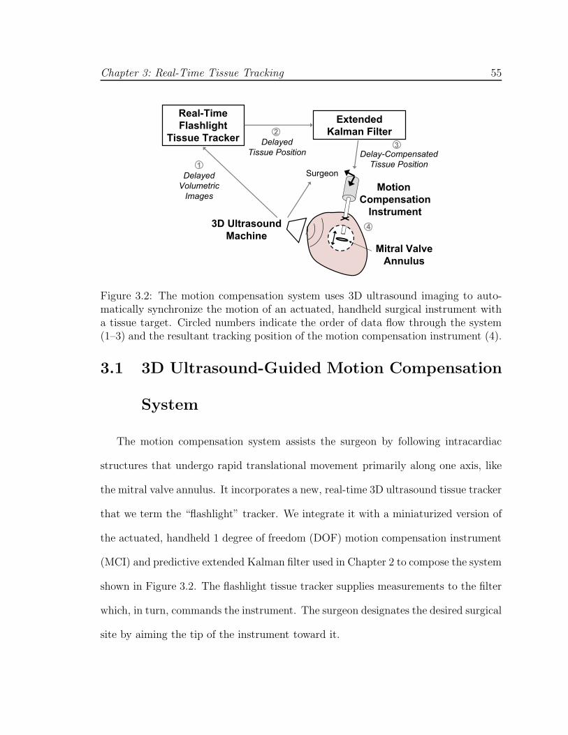
Chapter 3: Real-Time Tissue Tracking 55
Delayed
Tissue Position
Motion
Compensation
Instrument3D Ultrasound
Machine
Mitral Valve
Annulus
Extended
Kalman Filter
Delay-Compensated
Tissue Position
Real-Time
Flashlight
Tissue Tracker
Delayed
Volumetric
Images
Surgeon1
2
3
4
Figure 3.2: The motion compensation system uses 3D ultrasound imaging to auto-matically synchronize the motion of an actuated, handheld surgical instrument witha tissue target. Circled numbers indicate the order of data flow through the system(1–3) and the resultant tracking position of the motion compensation instrument (4).
3.1 3D Ultrasound-Guided Motion Compensation
System
The motion compensation system assists the surgeon by following intracardiac
structures that undergo rapid translational movement primarily along one axis, like
the mitral valve annulus. It incorporates a new, real-time 3D ultrasound tissue tracker
that we term the “flashlight” tracker. We integrate it with a miniaturized version of
the actuated, handheld 1 degree of freedom (DOF) motion compensation instrument
(MCI) and predictive extended Kalman filter used in Chapter 2 to compose the system
shown in Figure 3.2. The flashlight tissue tracker supplies measurements to the filter
which, in turn, commands the instrument. The surgeon designates the desired surgical
site by aiming the tip of the instrument toward it.

Chapter 3: Real-Time Tissue Tracking 56
Image
Slice
Modified
Radon
Transform
K-Means
Clustering
Active
Contour
Ultrasound
Volume Flashlight
Output:
Target
Position
Instrument Detection Target Segmentation
12
Figure 3.3: Data processing chain in the flashlight real-time tissue tracker. Circlednumbers correspond to those shown in Figure 3.2.
3.1.1 Real-Time 3D Ultrasound “Flashlight” Tissue Tracker
Figure 3.3 charts the data flow in the flashlight tracker. It consists of two consec-
utive operations: instrument detection followed by target segmentation. We employ
the modified Radon transform for real-time detection of the ray that passes through
the central axis of the instrument shaft [48]. Next, we distinguish between the target
and instrument along this ray. We construct an image slice through the ultrasound
volume that contains the instrument shaft. Pixels in the slice that exceed a grayscale
intensity threshold It are grouped into two clusters based on Euclidean distance us-
ing the K-means algorithm [1]. The value of It is empirically chosen to remove noise
and the mitral leaflets from the clustering. The resulting clusters roughly coincide
with the locations of the instrument and tissue target. A priori knowledge of the
ultrasound probe placement relative to the instrument and the tissue allows us to
designate the more distal cluster as the target.
Finally, an active contour is placed on the target cluster to segment its surface.
The active contour is governed by the minimization of the energy equation
E =∫
S(αEelastic + βEbending + γEimage)dS. (3.1)
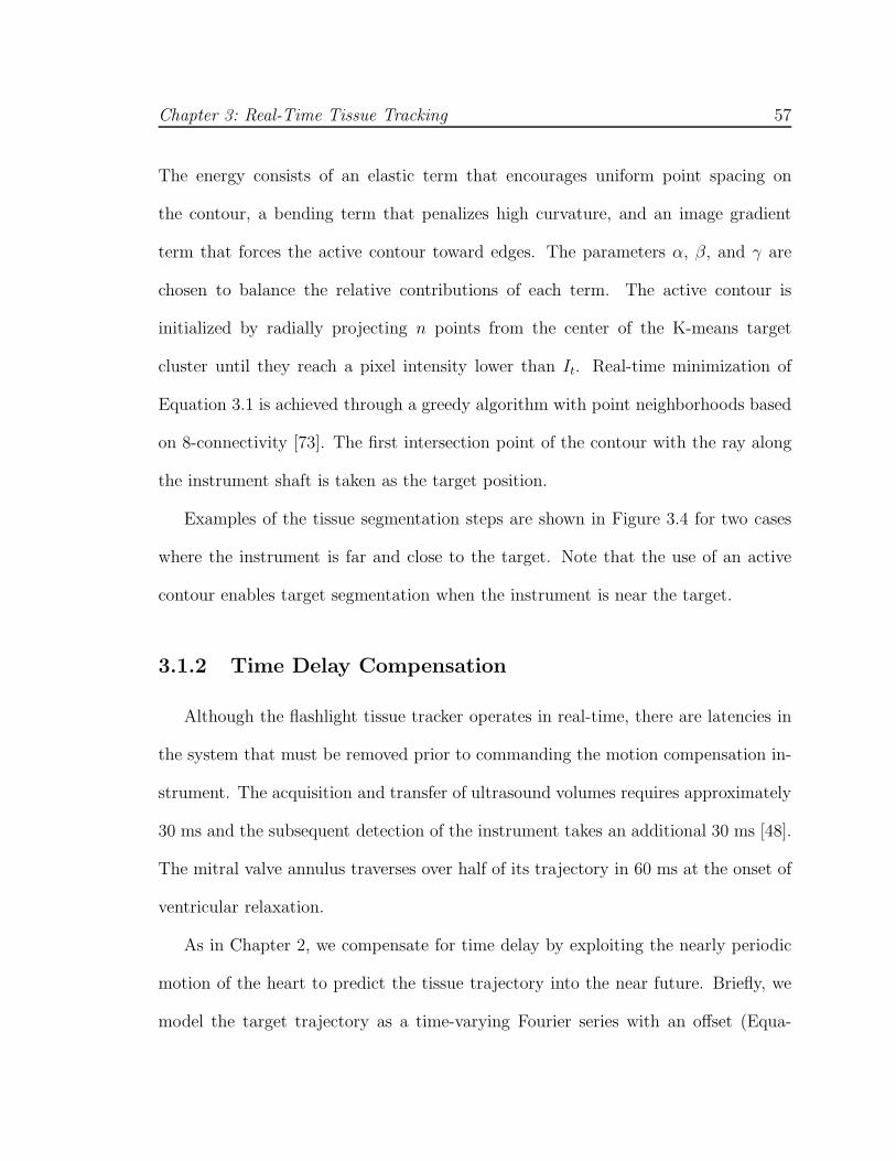
Chapter 3: Real-Time Tissue Tracking 57
The energy consists of an elastic term that encourages uniform point spacing on
the contour, a bending term that penalizes high curvature, and an image gradient
term that forces the active contour toward edges. The parameters α, β, and γ are
chosen to balance the relative contributions of each term. The active contour is
initialized by radially projecting n points from the center of the K-means target
cluster until they reach a pixel intensity lower than It. Real-time minimization of
Equation 3.1 is achieved through a greedy algorithm with point neighborhoods based
on 8-connectivity [73]. The first intersection point of the contour with the ray along
the instrument shaft is taken as the target position.
Examples of the tissue segmentation steps are shown in Figure 3.4 for two cases
where the instrument is far and close to the target. Note that the use of an active
contour enables target segmentation when the instrument is near the target.
3.1.2 Time Delay Compensation
Although the flashlight tissue tracker operates in real-time, there are latencies in
the system that must be removed prior to commanding the motion compensation in-
strument. The acquisition and transfer of ultrasound volumes requires approximately
30 ms and the subsequent detection of the instrument takes an additional 30 ms [48].
The mitral valve annulus traverses over half of its trajectory in 60 ms at the onset of
ventricular relaxation.
As in Chapter 2, we compensate for time delay by exploiting the nearly periodic
motion of the heart to predict the tissue trajectory into the near future. Briefly, we
model the target trajectory as a time-varying Fourier series with an offset (Equa-

Chapter 3: Real-Time Tissue Tracking 58
K-Means
Clustering
Image Slice
Active
Contour
A B
C D
E F
Instrument Shaft
Target
Instrument Shaft
Target
Figure 3.4: Outputs from each tissue segmentation step for examples where the in-strument is far and near the target (left and right columns, respectively). The imageslice through the instrument is shown in the top row. K-means clusters are shownas white and gray objects in the middle row. The segmented target shape (line) andtracking point (dot) are shown in the bottom row.
tion 2.5). We estimate the parameters of this model using an extended Kalman filter
(EKF). Because it is recursive, it is amenable to a real-time implementation. It has
the added benefit of providing noise reduction to the estimated target trajectory
through the regularization of the flashlight tracker measurements against the motion
model.
3.1.3 Motion Compensation Instrument
The motion compensation instrument (MCI) is a handheld surgical anchor deploy-
ment device that actively cancels the dominant 1D motion component of the mitral
valve annulus. Figure 3.5 shows the instrument, which is a miniaturized version of the
prototype from Chapter 2 that is compatible with the space limitations inside of the
operating room. It incorporates a voice coil linear motor (NCC10-15-023-1X, H2W

Chapter 3: Real-Time Tissue Tracking 59
Anchor
Driver
Linear MotorInstrument Shaft
Figure 3.5: The motion compensation instrument is a 1 DOF actuated anchor driverinstrument that is capable of tracking fast intracardiac structures.
Technologies, Valencia, CA, USA) for actuation of the anchor deployment stage up
to speeds and accelerations of 1.49 m/s and 103 m/s2 with a 25 mm range of motion.
A high linearity potentiometer (P3 America, San Diego, CA, USA) provides position
sensing. The instrument position is controlled with a slightly overdamped response
by a 1 kHz PID servo loop and has a -3 dB point of 35.0 Hz (-40 dB per decade
roll off rate). The overall weight of the instrument is 0.76 kg, which is less than 50%
of the weight of the original. Because of the reduced moving mass, the latency of
the instrument is lowered from 14 ms to 10 ms from the instrument in Chapter 2.
Weight reduction is achieved by using a smaller motor and light plastic materials for
construction.
3.1.4 System Implementation
The motion compensation system uses a dual CPU AMD Opteron 285 2.6 GHz
PC with 4 GB of RAM to process the ultrasound data and control the motion com-
pensation instrument. A 3D ultrasound machine (Sonos 7500, Philips Healthcare,

Chapter 3: Real-Time Tissue Tracking 60
Andover, MA, USA) streams volumes at 28 Hz to the PC over a 1 Gb LAN using
TCP/IP. A program written in C++ retrieves the ultrasound volumes and loads them
onto a GPU (7800GT, nVidia Corp, Santa Clara, CA, USA) for real-time instrument
axis detection. The GPU renders image slices through the instrument shaft that are
rotated to be horizontal through a trilinear interpolation. Subsequent flashlight tissue
tracking operations are done with a pixel intensity threshold of It = 50 and active
contour parameters n = 10, α = 0.5, β = 0.5, and γ = 1.0. Preliminary water tank
experiments indicate that the flashlight tracker is robust to changes in It and the
ratios between α, β, and γ up to or exceeding a factor of two. The EKF trains on 5 s
of flashlight position data and feeds-forward a tissue trajectory 78 ms ahead (68 ms
from image acquisition, transfer, and processing; 10 ms from instrument latency) to
the PID servo loop controlling the MCI. The instrument is powered by a BOP36-
1.5 M linear power amplifier (Kepco, Flushing, NY, USA). Real-time tissue tracking,
predictive filtering, and control algorithms are executed on the CPU.
3.2 Water Tank Validation
The accuracy and benefits of the motion compensation system were assessed
through a study of user performance in an in vitro beating heart surgical task. Ten
subjects (seven male, three female, aged 20–34) were instructed to use the MCI to
drive surgical anchors into a tissue phantom that simulated the motion of the mi-
tral valve annulus in a water tank. The MCI either provided motion compensation
through the system described in Section 3.1 or the MCI was set to act as a solid,
noncompensating instrument.

Chapter 3: Real-Time Tissue Tracking 61
3.2.1 Experimental Setup
The user trials were conducted in conditions that emulate those expected in a
beating heart mitral valve annuloplasty procedure. Figure 3.6 depicts the setup. Valve
motion was simulated by a cam follower mechanism that replicates the dominant 1D
motion component of the human mitral valve annulus that was determined in Chapter
2 (Figure 2.2). A tissue phantom of 2 cm thick polyethylene foam was affixed to a
load cell (Kistler, Spartanburg, SC, USA) that measured the forces applied by the
MCI during the task, then mounted to the cam and positioned in a water tank.
The cam simulated a heart beat of 60 beats per minute. The MCI was aligned at
roughly 15 deg to the motion axis of the target and contrained to move in 1 DOF
by a linear bearing guide rail. Subjects viewed the task through the monitor of the
3D ultrasound machine (SONOS 7500, Philips Medical, Andover, MA, USA). The
ultrasound probe was positioned to simultaneously image the target and instrument
and set approximately perpendicular to the target motion axis to mimic the probe
placement conditions in vivo. A potentiometer measured target position for off-line
assessment of system accuracy.
3.2.2 Testing Protocol
The subjects were instructed to deploy anchors into the moving tissue phantom
with the MCI in a series of trials. They were informed that the dual criteria for a suc-
cessful trial were that the anchor be securely deployed in the target and that the forces

Chapter 3: Real-Time Tissue Tracking 62
Motion
Compensation
Instrument
Foam Tissue
Target
3D Ultrasound Probe
Target Motion
Linear
Actuator
Water Tank
Force Sensor
User
Motion
Linear Bearing
Figure 3.6: Water tank setup for user trials
applied to the target by the MCI during the task not exceed 15 N1. As a secondary
goal, subjects were also told to try to minimize the contact forces experienced while
deploying the anchor. The subjects were taught to use the anchor driver mechanism
on the MCI and trained to recognize the “feeling” of forces up to 15 N when pushing
the MCI into a stationary target. When the subjects became confident in their sense
of the forces applied, they were given six practice anchoring trials with the moving
target: three with motion compensation and three with a solid instrument. After
training, the subjects proceeded to perform the task in ten trials (five with motion
compensation and five with a solid instrument) in randomized order. The outcome
of each anchor driving attempt and the amount of force applied was shared with the
subject directly after each trial.
115 N is the puncture force as determined in pilot studies on excised porcine mitral valve annulususing the MCI’s anchor driver mechanism. Puncture force will vary according to tissue propertiesas well as the geometry of the instrument tip.
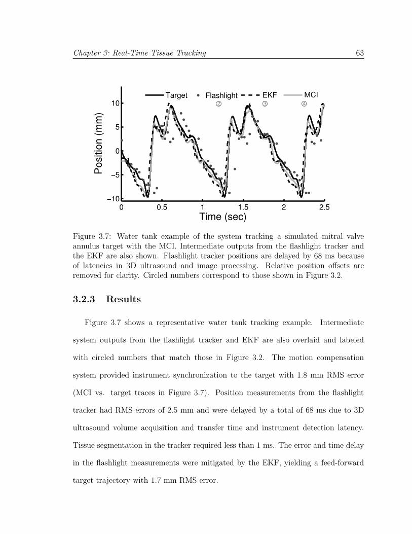
Chapter 3: Real-Time Tissue Tracking 63
Figure 3.7: Water tank example of the system tracking a simulated mitral valveannulus target with the MCI. Intermediate outputs from the flashlight tracker andthe EKF are also shown. Flashlight tracker positions are delayed by 68 ms becauseof latencies in 3D ultrasound and image processing. Relative position offsets areremoved for clarity. Circled numbers correspond to those shown in Figure 3.2.
3.2.3 Results
Figure 3.7 shows a representative water tank tracking example. Intermediate
system outputs from the flashlight tracker and EKF are also overlaid and labeled
with circled numbers that match those in Figure 3.2. The motion compensation
system provided instrument synchronization to the target with 1.8 mm RMS error
(MCI vs. target traces in Figure 3.7). Position measurements from the flashlight
tracker had RMS errors of 2.5 mm and were delayed by a total of 68 ms due to 3D
ultrasound volume acquisition and transfer time and instrument detection latency.
Tissue segmentation in the tracker required less than 1 ms. The error and time delay
in the flashlight measurements were mitigated by the EKF, yielding a feed-forward
target trajectory with 1.7 mm RMS error.

Chapter 3: Real-Time Tissue Tracking 64
Motion Compensation Solid0
20
40
60
80
100F
ailu
re R
ate
(%)
A
Motion Compensation Solid0
2
4
6
8
10
Con
tact
Tim
e (s
)
B
Figure 3.8: Mean failure rates (A) and mean continuous contact time (B) with motioncompensation and with a solid instrument. Error bars indicate standard error.
Motion compensated anchor driving provided a mean failure rate that was roughly
60% less than that observed for a solid instrument (Figure 3.8A). A statistically
significant difference between the means (26.0 ± 7.3% for motion compensation and
68.0±5.3% for a solid instrument, mean ± standard error) was apparent using a two-
sided t-test (p = 0.0002). It should be noted that a subset of four subjects obtained
0% failure rates with motion compensation and 70.0 ± 12.9% without. The three
engineers participating in the study belonged to this subset.
Motion compensation enabled the subjects to place the instrument in continuous
contact with the target for nearly three times longer than with a solid instrument (Fig-
ure 3.8B). On average, subjects kept constant contact on the target for 7.7 ± 0.6 sec
with motion compensation and 2.6 ± 0.2 sec without. This difference between the
means is statistically significant (p < 0.0001). The range of continuous contact times
observed over all motion compensation trials was 2.0–17.5 sec while the range for the
solid instrument was 0.7–7.9 sec.
The forces applied to the target were reduced for trials using motion compensation.

Chapter 3: Real-Time Tissue Tracking 65
5 10 150
20
40
Force (N)
Tim
e (
sec)
Motion Compensation Solid
MCI 95th
Solid 95th
Figure 3.9: Histogram of applied forces over all user trials. 95th percentiles are shown.
Figure 3.9 shows a histogram of force samples for all trials for the motion compensated
and solid instrument cases. The 95th percentile of forces for the solid instrument
(10.2 N) is nearly twice that seen for motion compensation (5.8 N).
3.3 In Vivo Animal Study
3.3.1 Experimental Setup
In vivo validation of the tracking performance of the system was performed in
a porcine beating heart model (Figure 3.10). Motion tracking was conducted in
two Yorkshire pigs during open chest, beating heart procedures. In each trial, the
tip of the MCI was inserted into the left atrial appendage and secured by a purse-
string suture. The ultrasound probe was positioned epicardially on the left side of
the heart to image the mitral valve and instrument. The surgeon was instructed to
aim the instrument tip toward a point on the mitral valve annulus and orient the
instrument shaft to align with the major motion axis of the annulus. Additionally,
during the second animal trial the surgeon attempted to manually track the annulus

Chapter 3: Real-Time Tissue Tracking 66
Figure 3.10: In vivo experiment setup.
with a stationary, noncompensating instrument. The surgeon was given three practice
attempts, followed by the actual trial. Motion tracking occurred for 20 s in each trial.
The 3D ultrasound images from the trials were recorded and manually segmented
to evaluate tracking performance. For each time-stamped volume, at least ten points
were selected for the cardiac tissue along the instrument axis. These were used to
calculate the centroid of the tissue target over time. Points in the left ventricle and on
the mitral leaflets were excluded. Segmentations were verified by a cardiac surgeon
with expertise in 3D ultrasound imaging and beating heart surgery.
The experimental protocol was approved by the Children’s Hospital Boston In-
stitutional Animal Care and Use Committee. All animals received humane care in
accordance with the 1996 Guide for the Care and Use of Laboratory Animals, recom-
mended by the US National Institute of Health.

Chapter 3: Real-Time Tissue Tracking 67
Animal Tracking Heart Rate RMS TrackingTrial No. Condition (bpm) Error (mm)
1 System 100 0.82 System 113 1.02 Manual 116 3.2
Table 3.1: In vivo tracking results for both animal trials. The second trial includedtracking with and without the motion compensation system.
3.3.2 Results
In vivo results indicate that the system provides accurate motion tracking under
surgical conditions. Figure 3.11A shows the tracking results for one of the in vivo
trials. Both the positions of the tissue target and instrument are shown. The system
tracked the target with a 1.0 mm RMS error while it beat at a spontaneous heart
rate of 113 bpm. Qualitatively, the tracking does not mimic the target trajectory
as faithfully as in the water tank case. A major contributor to this is the reduced
imaging quality in vivo. Figure 3.12 depicts the imaging conditions while tracking
over one heart cycle. Imaging artifacts and dropout are evident.
The system provided RMS tracking errors less than or equal to 1.0 mm in both
in vivo trials (Table 3.3.2). In contrast, manual tracking (Figure 3.11B) yielded RMS
errors of 3.2 mm on a slightly faster 116 bpm heart rate. The cross-correlation between
the trajectories of the target and instrument in this case suggests that the surgeon
lagged behind the target by approximately 339 ms. The RMS tracking error with
this delay removed would be 1.3 mm.

Chapter 3: Real-Time Tissue Tracking 68
30 32 34 36 38 40−5
0
5
Time (s)
Pos
ition
(m
m)
TissueInstrument A
0 2 4 6 8 10−5
0
5
Time (s)
Pos
ition
(m
m)
TissueInstrument B
Figure 3.11: In vivo tracking examples conducted with the motion compensationsystem (A) and manually (B). The manual tracking example is the last and bestattempt, after the surgeon had two training trials. The relative positional offsetsbetween the instrument and tissue target are removed for clarity.
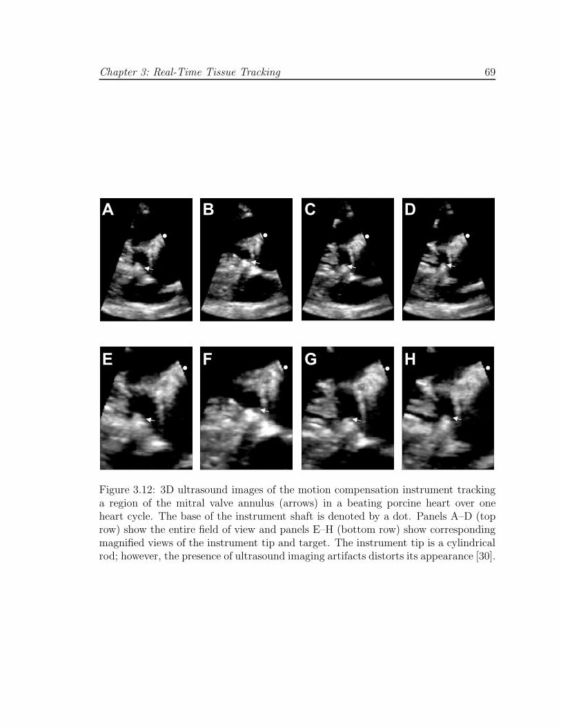
Chapter 3: Real-Time Tissue Tracking 69
A B C D
E F G H
Figure 3.12: 3D ultrasound images of the motion compensation instrument trackinga region of the mitral valve annulus (arrows) in a beating porcine heart over oneheart cycle. The base of the instrument shaft is denoted by a dot. Panels A–D (toprow) show the entire field of view and panels E–H (bottom row) show correspondingmagnified views of the instrument tip and target. The instrument tip is a cylindricalrod; however, the presence of ultrasound imaging artifacts distorts its appearance [30].
Chapter 3: Real-Time Tissue Tracking 70
3.4 Discussion
These experiments show that robotic motion tracking of beating, intracardiac tis-
sue is feasible in the surgical setting. Results from the in vivo study demonstrate that
robotic tracking of the mitral valve annulus can be achieved with low 1.0 mm RMS
error using standard 3D ultrasound imaging. This constitutes a 70% error reduction
when compared to manual attempts. The flashlight tissue tracker proved to be robust
to in vivo imaging artifacts, dropout, and noise by exploiting the spatial coherence
of the instrument in ultrasound to pinpoint the tissue target. High accuracy motion
tracking was achieved in the presence of significant delay and noise by regularizing
position measurements against the cyclic motion of the heart with a predictive ex-
tended Kalman filter. Water tank results show that the filter reduces noise by 30%
while simultaneously removing the overall system delay of 78 ms.
Using the system in an in vitro surgical anchor deployment task, subjects achieved
success rates that were more than double those achieved with a non-compensated
instrument. Furthermore, the system permitted more careful placement of the anchors
by reducing the forces applied and extending the continuous contact time between the
instrument and the target. While motion compensated anchor driving had relatively
low failure rates, we anticipate that it can be driven to nearly zero with additional
user training and a small modification to the instrument. The perfect performance
of users with technology experience (e.g., engineers) suggests that the other users
could benefit from more practice. Indeed, several users were confused by ultrasound
visualization and impaired by the inertial forces resulting from the actuator’s moving
mass, which could be difficult to distinguish from contact forces. This led to cases

Chapter 3: Real-Time Tissue Tracking 71
where the user would not push the instrument firmly into contact with the target.
Modification of the instrument to include a counterbalancing mass may mitigate the
loss in haptic feedback that results from inertial effects.
Prior research has shown that humans cannot track the heart when it is beating
faster than 60 bpm [18, 32]. The preliminary in vivo manual tracking results of this
chapter suggest that the main reason for this is the presence of a large lag that puts the
instrument motion out of phase with the heart. For the cardiac surgeon in this study,
we estimate this lag to be 339 ms on a heart beating at 116 bpm. This is consistent
with the lags measured by Jacobs et al. for tasks against simulated heart motion at
35 and 60 bpm [32]. A retrospective analysis of the manual tracking trial suggests
that the surgeon was able to match the frequency and amplitude of the annular
trajectory reasonably well – to 1.3 mm RMS error when corrected for the 339 ms
lag. It is unlikely that training will reduce the lag to levels low enough to achieve
accurate manual tracking: human visual processing requires roughly 150 ms [63] and,
as discussed above, even a 60 ms delay is intolerable for motion compensation. The
surgeon could conceivably predict the tissue trajectory and feed-forward its motion
like the strategy with the extended Kalman filter. However, even if possible, this
would not be a clinically viable approach because it would severely limit the surgeon’s
ability to attend to the other aspects of the procedure.
The difficulty with manual heart tracking has inspired a number of parallel efforts
in motion compensation for external heart procedures like coronary artery bypass
graft. Nakamura et al. demonstrated automatic tracking of a laser point moving like
the external heart wall with a 4 DOF robot guided by two high speed cameras [44].

Chapter 3: Real-Time Tissue Tracking 72
Later, Ginhoux et al. provided an in vivo demonstration with a modified 6 DOF
AESOP robot guided by a high-speed camera to track LEDs affixed to a beating
porcine heart [24]. Similarly, Bebek and Cavusolgu used a 6 DOF PHANTOM robot
to track sonomicrometry sensors sutured to the heart surface [6]. Because these sys-
tems function outside of the heart, they are able to achieve excellent results by using
relatively large robots with fast (257–955 Hz) and accurate (250–330 µm) positioning
sensors that either track fiducials or are placed onto the surgical target.
Limited by the constraints of operating inside the heart, the system in this work
uses relatively low-frequency (28 Hz) and noisy (0.5 mm) 3D ultrasound imaging to
directly track heart tissue. We also adopt a simplified 1 DOF robot that can function
within the restricted space of the heart. Using this system in a beating porcine heart,
we show a 70% decrease in error compared to manual tracking. We anticipate a
larger benefit in the human heart because the human mitral valve annulus undergoes a
larger excursion (10–18 mm) [70, 20] than was seen in the porcine model here (6 mm).
However, the in vivo and in vitro studies suggest two potential improvements to the
system. First, adding a low frequency term to the motion model in the filter would
improve tracking the small, slowly-varying motion component seen in the in vivo
result (Figure 3.11A) that is due to respiration. A second improvement, and the
subject of the next chapter, is the modification of the robot controller to explicitly
regulate the interaction forces between the robot and tissue to increase the saftey of
the system. Although the forces measured in the in vitro anchor deployment task of
Section 3.2 were roughly half those seen with a non-compensated instrument, large
force excursions in excess of 5 N were still present (Figure 3.9). The tearing force for

Chapter 3: Real-Time Tissue Tracking 73
in vivo heart tissue while deploying a surgical anchor is approximately 8 N2 and for
safety the surgeon tries to maintain forces that are below 3 N.
2This force was determined using the MCI anchor driver mechanism on freshly excised porcineheart. The force will vary according to the tissue properties as well as the geometry of the instrumenttip.

Chapter 4
Force Tracking with Feed-Forward
Motion Estimation
The motion of the heart during beating heart surgery makes it difficult to apply
precise forces for procedures like mitral valve annuloplasty. Anchor deployment trials
from Chapter 3 demonstrate that this is the case even when using a position tracking
motion compensation system: the system helps reduce contact forces but there are
still fluctuations that can reach dangerous levels. There are a number of difficulties
associated with using a positional controller during sustained contact against moving
tissue. First, small errors in the estimated target position can cause the robot to
interact with the tissue at high forces. Second, when in contact, the surgical target is
shadowed by the instrument in 3D ultrasound and identifying its position accurately is
challenging. Finally, because the robot is much stiffer than the heart, contact causes
the tissue to comply with the location of the robotic instrument tip. Having the
robot follow the position of the tissue in this state would not provide good motion
74

Chapter 4: Force Tracking with Feed-Forward Motion Estimation 75
compensation because the tissue location is forced by the robot. As an extreme
illustration of this point, consider the case of the robot pushing the tissue until it is
fully restrained from moving. Tracking the stationary position of the tissue in this
case would not have the desired effect from motion compensation.
A force control approach is more appropriate when attempting to manipulate
beating heart tissue. Previous work on surgical force control has largely focused on
force feedback for teleoperation of surgical instruments and robots (reviewed in [50]).
Force feedback has demonstrated a number of performance benefits in the execution
of remote surgical tasks [55, 38, 69] and can enhance safety when used to implement
virtual workspace limits [28, 67]. In this setting, the primary role of the force controller
is to provide haptic information to the user while the user commands the robot to
interact with the surgical target.
In contrast, beating heart applications require the robot controller to autonomously
maintain prescribed forces of the instrument against the target tissue despite its fast
motion. One major concern is safety, given the well-documented occurrence of insta-
bility in force control [72, 16, 17, 2, 13]. A robotic system for beating heart surgery
must be damped and stable to ensure that it will not overshoot or oscillate in response
to changes in the desired force trajectory or sudden target motions. Furthermore, the
system must have sufficient bandwidth to reject the disturbance caused by heart
motion. Previous research indicates that standard force control strategies can only
achieve stability for low closed-loop bandwidths due to vibratory modes in the robot
structure [16, 17, 2, 13]. These findings were obtained in the context of large indus-
trial robots interacting with stiff targets. To ensure adequate robot performance and
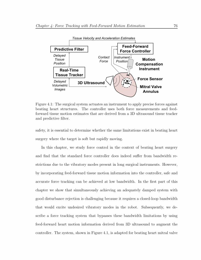
Chapter 4: Force Tracking with Feed-Forward Motion Estimation 76
Delayed
Tissue
PositionMotion
Compensation
Instrument
3D UltrasoundMitral Valve
Annulus
Predictive FilterFeed-Forward
Force Controller
Tissue Velocity and Acceleration Estimates
Real-Time
Tissue Tracker
Instrument
Position
Force Sensor
Contact
Force
Delayed
Volumetric
Images
Figure 4.1: The surgical system actuates an instrument to apply precise forces againstbeating heart structures. The controller uses both force measurements and feed-forward tissue motion estimates that are derived from a 3D ultrasound tissue trackerand predictive filter.
safety, it is essential to determine whether the same limitations exist in beating heart
surgery where the target is soft but rapidly moving.
In this chapter, we study force control in the context of beating heart surgery
and find that the standard force controller does indeed suffer from bandwidth re-
strictions due to the vibratory modes present in long surgical instruments. However,
by incorporating feed-forward tissue motion information into the controller, safe and
accurate force tracking can be achieved at low bandwidth. In the first part of this
chapter we show that simultaneously achieving an adequately damped system with
good disturbance rejection is challenging because it requires a closed-loop bandwidth
that would excite undesired vibratory modes in the robot. Subsequently, we de-
scribe a force tracking system that bypasses these bandwidth limitations by using
feed-forward heart motion information derived from 3D ultrasound to augment the
controller. The system, shown in Figure 4.1, is adapted for beating heart mitral valve

Chapter 4: Force Tracking with Feed-Forward Motion Estimation 77
Linear Motor
Force
Sensor
Fiber Optic
Cables
Anchor
Driver
Instrument Shaft
Figure 4.2: The motion compensation instrument (MCI) is a handheld surgical anchordeployment device. It is actuated in one degree of freedom to cancel the dominant 1Dmotion component of the mitral valve annulus. A tip-mounted optical force sensor [74]measures contact forces against beating heart tissue.
annuloplasty. It uses the motion compensation instrument (MCI) from Chapter 3
that can follow the rapid, nearly uniaxial motion of the mitral valve annulus. An
optical force sensor [74] is integrated into the tip of the instrument (Figure 4.2) to
provide measurements of the interaction forces with the surgical target. We validate
the system and demonstrate its utility to the surgeon in an in vivo experiment in a
large animal model.
4.1 Rigid Body Analysis
To gain some insight into the use of force control in beating heart surgery, we first
consider the case of a perfectly rigid robotic instrument. The robot is modeled as a
mass m and damper b subjected to a commanded actuator force fa and environment
contact force fe. The damper b captures the effects of friction in the robot, friction at
the insertion point to the heart, and fluid motion. Approximating the environment

Chapter 4: Force Tracking with Feed-Forward Motion Estimation 78
Motion compensation instrument
(Rigid model)
Beating heart target
Figure 4.3: Rigid body robot model in contact with an actively moving, compliantenvironment.
as a spring of stiffness ke yields the system dynamics
mx + bx = fa − ke(x − xe), (4.1)
where x is the instrument tip position and xe is the desired tissue target position
(i.e., its position if it were not deformed by contact). The model is illustrated in
Figure 4.3. For simplicity, we neglect force sensor compliance in the model because
it is significantly stiffer than the tissue environment.
Now consider a standard force regulator control law [58]
fa = fd + Kf(fd − fe) − Kvx, (4.2)
where Kf and Kv are controller gains and fd is the desired force. Combining Equa-
tions 4.1 and 4.2 and applying the Laplace transform gives the closed-loop contact
force relationship
Fe(s) = T (s)Fd(s) + Z(s)Xe(s), (4.3)
where the force tracking transfer function T (s) and robot impedance transfer function

Chapter 4: Force Tracking with Feed-Forward Motion Estimation 79
Z(s) are
T (s) ,Fe(s)
Fd(s)=
ke
m(1 + Kf)
C(s), (4.4)
Z(s) ,Fe(s)
Xe(s)= −kes(s + Kv+b
m)
C(s), (4.5)
C(s) = s2 +Kv + b
ms +
ke
m(1 + Kf). (4.6)
Equation 4.3 makes explicit that the target motion xe is a disturbance that perturbs
fe from fd.
Controller gains Kf and Kv are chosen to ensure system stability, sufficient damp-
ing, and good rejection of xe. The last is achieved by designing Z(s) to have small
magnitude in the bandwidth of Xe(s). For the mitral valve annulus, which is essen-
tially bandlimited to approximately 15 Hz (Figure 2.3), this is equivalent to setting the
impedance corner frequency fz greater than or equal to 15 Hz. Figure 4.4 depicts typ-
ical mitral valve annulus motion and its effect on the contact force for various fz based
on simulations of Equations 4.3–4.5 with fd = 0. Parameter values of m = 0.27 kg,
b = 18.0 Ns/m, and ke = 133 N/m are assumed based on system identification of
the MCI and preliminary estimates of the mitral valve annulus stiffness. As will be
shown shortly, obtaining a large impedance corner frequency fz is synonymous with
increasing the natural frequency fn of the closed-loop system, which is also equivalent
to increasing Kf .
First, using second order system design techniques [49] on the characteristic equa-
tion in Equation 4.6 gives the natural frequency fn and damping ζ of the system

Chapter 4: Force Tracking with Feed-Forward Motion Estimation 80
1 1.5 2 2.5 3
−0.2
−0.1
0
0.1
0.2
0.3
0.4
0.5
Time (s)
For
ce (
N)
1 1.5 2 2.5 3−10
−5
0
5
10
Time (s)P
ositi
on (
mm
)
100
101
102
0
10
20
30
40
50
|Z(jf
)| (
dB)
f (Hz)
fz=5 Hz f
z=15 Hz f
z=50 Hz
fz=5 Hz f
z=15 Hz f
z=50 Hz
A
B
C
Figure 4.4: The effect of mitral valve annulus motion on contact forces. Humanmitral valve annulus trajectory (A) and corresponding force disturbances for fz of 5,15, and 50 Hz (B). The magnitude plots of the impedance transfer function |Z(jf)| areshown with corner frequencies marked by squares (C). Gain settings are Kf = 27.5,Kv = 45.9 for fz = 5 Hz; Kf = 255.2, Kv = 173.8 for fz = 10 Hz; and Kf = 2845.7,Kv = 621.4 for fz = 50 Hz. Mitral valve annulus motion data is repeated fromChapter 2.
as
fn =1
2π
√
ke
m(1 + Kf), (4.7)
ζ =Kv + b
4πmfn. (4.8)
To avoid potentially dangerous overshoot, we set the system to be critically damped (ζ =

Chapter 4: Force Tracking with Feed-Forward Motion Estimation 81
1.0) and manipulate Equations 4.5, 4.7, and 4.8 to show that for any impedance trans-
fer function of the form
Z(s) ∝ s(s + 4πfn)
s2 + 4πfns + (2πfn)2(4.9)
the natural frequency fn is a function of the impedance corner frequency fz by
fn =
(√208 − 14
6
)− 1
2
fz ≈ 3.7698fz. (4.10)
Hence, while a position regulator can follow a trajectory bandlimited to 15 Hz with
about the same closed-loop natural frequency, a force regulator must have a natural
frequency of approximately 57 Hz to follow the same motion. This indicates that the
force regulator inherently requires high bandwidth to compensate for target motion.
Figure 4.5 shows the system damping and impedance corner frequency over a
range of values for Kf and Kv. It is clear that there is a trade-off between the
two performance criteria: increasing Kf increases the corner frequency but decreases
damping; the opposite is true for Kv. Because of this trade-off, achieving suitable
disturbance rejection (fz ≥ 15 Hz) while maintaining damping (ζ ≥ 1) requires
large gains. From Equations 4.7–4.10 we calculate gain settings of Kf = 255.2 and
Kv = 173.8 to set the system to be critically damped with fz = 15 Hz, assuming that
the rigid body model is appropriate at such high gains.
4.2 Bandwidth Contraints due to Robot Dynamics
In this section, we study the effect of high gains on robot performance. Extensive
prior work on force control has delineated a number of instabilities that can arise in
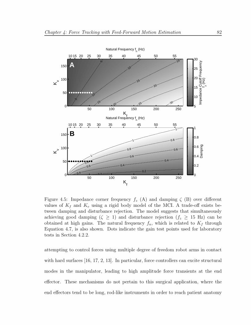
Chapter 4: Force Tracking with Feed-Forward Motion Estimation 82
10 15 20 25 30 35 40 45 50 55
Natural Frequency fn (Hz)
Kf
Kv
5
5
10
10
15
15
15
20
20
25 30
50 100 150 200 2500
50
100
150
Impe
danc
e C
utof
f Fre
quen
cyf z (
Hz)
5
10
15
20
25
30
10 15 20 25 30 35 40 45 50 55
Natural Frequency fn (Hz)
Kf
Kv
0.20.2
0.4
0.4
0.4
0.6
0.6
0.6
0.8
0.8
0.8
1
1
1
50 100 150 200 2500
50
100
150
Dam
ping
z
0
0.2
0.4
0.6
0.8
1
B
A
Figure 4.5: Impedance corner frequency fz (A) and damping ζ (B) over differentvalues of Kf and Kv using a rigid body model of the MCI. A trade-off exists be-tween damping and disturbance rejection. The model suggests that simultaneouslyachieving good damping (ζ ≥ 1) and disturbance rejection (fz ≥ 15 Hz) can beobtained at high gains. The natural frequency fn, which is related to Kf throughEquation 4.7, is also shown. Dots indicate the gain test points used for laboratorytests in Section 4.2.2.
attempting to control forces using multiple degree of freedom robot arms in contact
with hard surfaces [16, 17, 2, 13]. In particular, force controllers can excite structural
modes in the manipulator, leading to high amplitude force transients at the end
effector. These mechanisms do not pertain to this surgical application, where the
end effectors tend to be long, rod-like instruments in order to reach patient anatomy

Chapter 4: Force Tracking with Feed-Forward Motion Estimation 83
through small ports, and tissues are highly compliant.
It is well known, however, that axial motion of such long rods excites transverse
vibrations [31]. The dynamics describing this motion are nonlinear and have time
varying parameters, but for the purposes of developing effective force controllers it
is not necessary to model these dynamics: we need only to determine the frequency
at which they become significant so that reasonable bandwidth restrictions can be
imposed on the rigid body model and closed-loop system analysis of the preceding
section. While structural resonance can be used to enhance performance in some
situations, it is typically avoided because inadvertent excitation of the resonance can
destabilize the controller, reduce the positional accuracy of the instrument, and cause
undue wear to the robot. In the present application, resonance can further cause
injury to the patient from the transmission of vibrational energy to the tissue in
contact with the robot.
In the following section, we analytically and empirically demonstrate that vibra-
tion precludes the use of the high gain force regulator suggested in Figure 4.5. We first
demonstrate that vibration occurs at relatively low frequency for surgical robots with
long instruments. Subsequently, we empirically demonstrate that these vibrations are
significant in the motion compensation system and can lead to instability as Kf is
increased until the natural frequency approaches the resonance of the instrument.
4.2.1 Gain Limit to Avoid Vibration
Consider a cylindrical rod of length l and radius r undergoing axial motion while
compressed by a force fe (Figure 4.6). At low velocities, the fundamental mode of
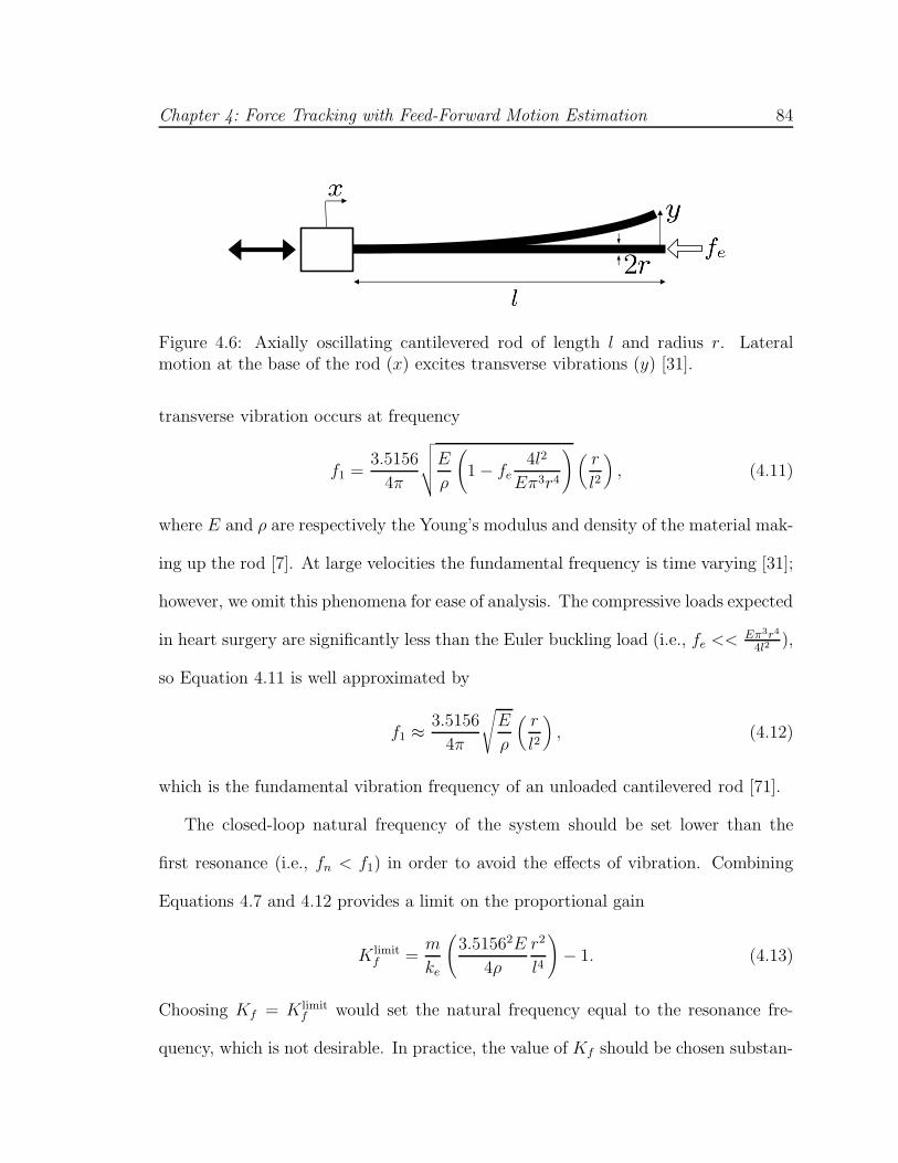
Chapter 4: Force Tracking with Feed-Forward Motion Estimation 84
Figure 4.6: Axially oscillating cantilevered rod of length l and radius r. Lateralmotion at the base of the rod (x) excites transverse vibrations (y) [31].
transverse vibration occurs at frequency
f1 =3.5156
4π
√
√
√
√
E
ρ
(
1 − fe4l2
Eπ3r4
)
(
r
l2
)
, (4.11)
where E and ρ are respectively the Young’s modulus and density of the material mak-
ing up the rod [7]. At large velocities the fundamental frequency is time varying [31];
however, we omit this phenomena for ease of analysis. The compressive loads expected
in heart surgery are significantly less than the Euler buckling load (i.e., fe << Eπ3r4
4l2),
so Equation 4.11 is well approximated by
f1 ≈3.5156
4π
√
E
ρ
(
r
l2
)
, (4.12)
which is the fundamental vibration frequency of an unloaded cantilevered rod [71].
The closed-loop natural frequency of the system should be set lower than the
first resonance (i.e., fn < f1) in order to avoid the effects of vibration. Combining
Equations 4.7 and 4.12 provides a limit on the proportional gain
K limitf =
m
ke
(
3.51562E
4ρ
r2
l4
)
− 1. (4.13)
Choosing Kf = K limitf would set the natural frequency equal to the resonance fre-
quency, which is not desirable. In practice, the value of Kf should be chosen substan-

Chapter 4: Force Tracking with Feed-Forward Motion Estimation 85
tially lower than K limitf so that the gain of the closed-loop system is small through
the spectral extent of the resonance.
The MCI is mounted with a stainless steel 14 gauge blunt needle (E = 200 GPa,
ρ = 7900 kg/m3, r = 1.1 mm) with an inner stainless steel push rod used for anchor
deployment in mitral valve annuloplasty [68, 65, 66]. Its length is l = 22.8 cm1. For
simplicity we approximate the entire structure as a solid cylindrical rod. Assuming
the same system parameters as before, Equations 4.12 and 4.13 predict that the
fundamental resonance occurs at f1 = 27.6 Hz and the limit on the proportional gain
is K limitf = 60.4. Referring to the rigid body performance plots in Figure 4.5, it is
clear that the controller gains cannot be set high enough to simultaneously avoid
resonance and meet the criteria of a damped system with high bandwidth.
Because K limitf increases quadratically with r, increasing the radius of the instru-
ment substantially would permit high gain without exciting vibration. However, for
minimally invasive surgical procedures, the instrument width should be kept small in
order to minimize the sizes of the ports into the thorax and heart. Clincal researchers
have also found that the sizes of standard robotic instruments (2.5 mm ≤ r ≤ 5.5 mm)
are a limiting factor in accessing and manipulating mitral valve anatomy [39, 19].
LaPietra et al. found that thinner robotic instruments (r = 1.9 mm) improved ac-
cess in stopped-heart mitral valve annuloplasties performed in a canine model [39].
Figure 4.7 depicts f1 and K limitf over a range of r for the system.
1Preliminary animal testing found this to be the minimum length necessary for the instrument toaccess the mitral valve during beating heart procedures in a porcine model. The instrument approachwas from the left atrial appendage through the second intercostal space in a left thoracotomy.

Chapter 4: Force Tracking with Feed-Forward Motion Estimation 86
0.5 1 1.5 20
50
100
150
200
250
Radius of instrument (mm)K
flimit
0.5 1 1.5 215
20
25
30
35
40
45
50
55
Radius of instrument (mm)
Res
onan
ce F
requ
ency
(H
z)
Figure 4.7: Transverse vibration limits the maximum allowable proportional gain Kf .The resonance frequency f1 (A) and resulting upper limit K limit
f (B) are shown overthe radius of the instrument r. The values corresponding to a 14 gauge needle likethat mounted on the MCI are indicated with circles. The instrument is assumed to besteel (E = 200 GPa, ρ = 7900 kg/m3) with length l = 22.8 cm. All other parametersare the same as before.
4.2.2 Experimentally Observed Vibration and Instability
Although avoiding vibratory motion in a surgical robot is intuitively appealing, it
remains unclear if such motion is severe enough to present a problem in beating heart
surgery. Here we experimentally demonstrate that these vibrations can affect the
accuracy of the instrument tip position and also lead to unstable behavior. We fur-
thermore validate Equations 4.12 and 4.13 for predicting the fundamental resonance
frequency and gain limit K limitf , respectively.
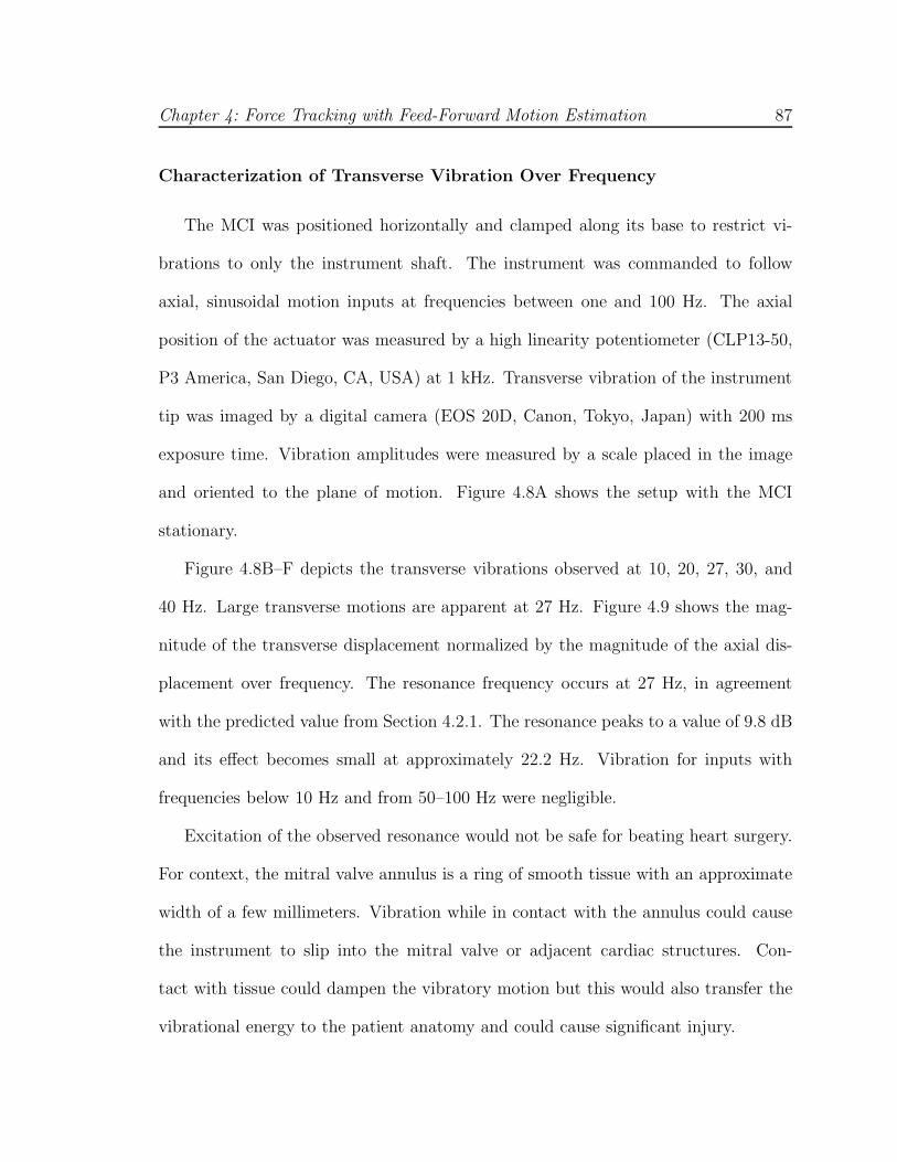
Chapter 4: Force Tracking with Feed-Forward Motion Estimation 87
Characterization of Transverse Vibration Over Frequency
The MCI was positioned horizontally and clamped along its base to restrict vi-
brations to only the instrument shaft. The instrument was commanded to follow
axial, sinusoidal motion inputs at frequencies between one and 100 Hz. The axial
position of the actuator was measured by a high linearity potentiometer (CLP13-50,
P3 America, San Diego, CA, USA) at 1 kHz. Transverse vibration of the instrument
tip was imaged by a digital camera (EOS 20D, Canon, Tokyo, Japan) with 200 ms
exposure time. Vibration amplitudes were measured by a scale placed in the image
and oriented to the plane of motion. Figure 4.8A shows the setup with the MCI
stationary.
Figure 4.8B–F depicts the transverse vibrations observed at 10, 20, 27, 30, and
40 Hz. Large transverse motions are apparent at 27 Hz. Figure 4.9 shows the mag-
nitude of the transverse displacement normalized by the magnitude of the axial dis-
placement over frequency. The resonance frequency occurs at 27 Hz, in agreement
with the predicted value from Section 4.2.1. The resonance peaks to a value of 9.8 dB
and its effect becomes small at approximately 22.2 Hz. Vibration for inputs with
frequencies below 10 Hz and from 50–100 Hz were negligible.
Excitation of the observed resonance would not be safe for beating heart surgery.
For context, the mitral valve annulus is a ring of smooth tissue with an approximate
width of a few millimeters. Vibration while in contact with the annulus could cause
the instrument to slip into the mitral valve or adjacent cardiac structures. Con-
tact with tissue could dampen the vibratory motion but this would also transfer the
vibrational energy to the patient anatomy and could cause significant injury.

Chapter 4: Force Tracking with Feed-Forward Motion Estimation 88
A
E
B
F
C D
0 Hz (Stationary) 10 Hz
20 Hz 27 Hz
30 Hz 40 Hz
Figure 4.8: Instrument with force sensor at rest (A) and vibrating due to an axial,sinusoidal motion at 10 Hz (B), 20 Hz (C), 27 Hz (D), 30 Hz (E), and 40 Hz (F)imposed at the base of the instrument shaft. Transverse vibration is maximal at27 Hz, the predicted resonance frequency from Section 4.2.1. Exposure times are200 ms. Scale marks at right are in millimeter.
Force Regulator Instability at High Gain
In this experiment we study the effect of vibration on stability by testing increasing
values of Kf that approach the predicted K limitf = 60.4 from Section 4.2.1. This is
equivalent to testing the system at increasing natural frequencies that approach the
27 Hz resonance of the MCI.
As before, the MCI was positioned horizontally on a flat surface and clamped along
its body to restrict vibrations to only the instrument shaft. The instrument tip was
placed in series with a steel leaf spring with a stiffness matched to the approximate
stiffness of the mitral valve annulus (ke = 133 N/m). The desired force fd was a unit

Chapter 4: Force Tracking with Feed-Forward Motion Estimation 89
10 15 20 25 30 35 40 45 50−20
−15
−10
−5
0
5
10
Frequency (Hz)
Tra
nsve
rse
Mot
ion
Gai
n (d
B)
0 dB
22.17 Hz
Figure 4.9: Magnitude of transverse displacement normalized by the magnitude ofthe axial displacement (y and x, respectively, as shown in Figure 4.6). As predictedin Section 4.2.1, the resonance occurs at 27 Hz. The estimated 0 dB frequency ismarked.
0 0.2 0.4 0.6 0.8 1 1.20
1
2
Time (s)
For
ce (
N)
0 0.2 0.4 0.6 0.8 1 1.20
1
2
Time (s)
For
ce (
N)
0 0.2 0.4 0.6 0.8 1 1.20
1
2
Time (s)
For
ce (
N)
A
C
B
Figure 4.10: Stable and unstable step response examples: Kf = 5 and stable (A);Kf = 40 and stable but underdamped (B); Kf = 50 and unstable (C).
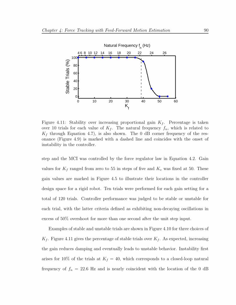
Chapter 4: Force Tracking with Feed-Forward Motion Estimation 90
4 6 8 10 12 14 16 18 20 22 24 26
Natural Frequency fn (Hz)
0 10 20 30 40 50 600
20
40
60
80
100
Kf
Sta
ble
Tria
ls (
%)
Figure 4.11: Stability over increasing proportional gain Kf . Percentage is takenover 10 trials for each value of Kf . The natural frequency fn, which is related toKf through Equation 4.7), is also shown. The 0 dB corner frequency of the res-onance (Figure 4.9) is marked with a dashed line and coincides with the onset ofinstability in the controller.
step and the MCI was controlled by the force regulator law in Equation 4.2. Gain
values for Kf ranged from zero to 55 in steps of five and Kv was fixed at 50. These
gain values are marked in Figure 4.5 to illustrate their locations in the controller
design space for a rigid robot. Ten trials were performed for each gain setting for a
total of 120 trials. Controller performance was judged to be stable or unstable for
each trial, with the latter criteria defined as exhibiting non-decaying oscillations in
excess of 50% overshoot for more than one second after the unit step input.
Examples of stable and unstable trials are shown in Figure 4.10 for three choices of
Kf . Figure 4.11 gives the percentage of stable trials over Kf . As expected, increasing
the gain reduces damping and eventually leads to unstable behavior. Instability first
arises for 10% of the trials at Kf = 40, which corresponds to a closed-loop natural
frequency of fn = 22.6 Hz and is nearly coincident with the location of the 0 dB

Chapter 4: Force Tracking with Feed-Forward Motion Estimation 91
corner frequency for the observed resonance (Figure 4.9). Increasing Kf to 50 and
above leads to 100% of the trials being unstable. This is less than the predicted
upper bound of K limitf = 60.4 but is nonetheless expected because of the spectral
width of the resonance seen in Figure 4.9. Overall, these results suggest that exciting
vibrational modes in even a single degree of freedom robot can lead to an unstable,
unsafe controller.
4.3 Force Control with Feed-Forward Target
Motion
The preceding sections indicate that vibrational modes in surgical instruments
prevent the high gain settings required for a force regulator to obtain both damping
and good heart motion rejection. Rather than use a pure force error feedback control
strategy, an alternative strategy employs feed-forward target motion information in
the controller. Previous work has shown that this approach can improve force tracking
when dealing with moving or uneven surfaces [56, 33]. This approach is well suited
to beating heart applications because accurate predictions of heart motion can be
obtained by exploiting its periodicity [62, 51, 24, 6, 21].
Consider the control law
fa = fd + Kf(fd − fe) + Kv( ˆxe − x) + b ˆxe + m ˆxe, (4.14)
which is Equation 4.2 augmented with feed-forward estimates of the target velocity
ˆxe and acceleration ˆxe. The contact force relationship in Equation 4.3 becomes
Fe(s) = T (s)Fd(s) − Z(s)(
Xe(s) − Xe(s))
,

Chapter 4: Force Tracking with Feed-Forward Motion Estimation 92
where T (s) and Z(s) are defined as before in Equations 4.4 and 4.5, respectively.
Observe that the use of feed-forward terms ˆxe and ˆxe enable the cancellation of the
motion disturbance xe without the need to greatly increase the natural frequency
of the system. The controller can then be designed with a low closed-loop natural
frequency to avoid the effects of vibration and other high order dynamics that lead
to reduced damping and instability. The feed-forward bandwidth is set equal to
the bandwidth of the heart motion disturbance, which is lower than the resonance
frequency of the robot.
4.4 Tissue Motion Estimation with 3D Ultrasound
To obtain the motion terms needed in the feed-forward controller, we first deter-
mine the position of the tissue in 3D ultrasound using the real-time tissue segmen-
tation algorithm from Chapter 3. The algorithm takes advantage of the high spatial
coherence of the instrument, which appears as a bright and straight object in the
volume, to designate the tissue target. Figure 4.12 depicts using this method to track
a point on the mitral valve annulus in a beating porcine heart.
As in the previous chapters, we model the nearly uniaxial motion of the mitral
valve annulus as a time-varying Fourier series with an offset and truncated to m
harmonics (Equation 2.5). For clarity, we repeat the motion model using the notation
of this chapter:
xe(t) = c(t) +m∑
i=1
ri(t) sin(θi(t)),
where c(t) is the offset, ri(t) are the harmonic amplitudes, and θi(t) , i∫ t0 ω(τ)dτ +
φi(t), with heart rate ω(t) and harmonic phases φi(t). Prior to contact, measure-

Chapter 4: Force Tracking with Feed-Forward Motion Estimation 93
3DUS Tissue Tracking
• Anchors successfully driven into
Motion
Compensation
Instrument
Annulus
Point
Figure 4.12: Slice through real-time 3D ultrasound volume showing tissue tracking.Squares denote the instrument with tip-mounted force sensor and the surgical targetlocated on the mitral valve annulus.
ments from the tissue tracker are used to train an extended Kalman filter to provide
estimates of the model parameters c(t), ri(t), ω(t), and θi(t). These parameters are
used to generate smooth feed-forward velocity and acceleration terms for the force
controller of Equation 4.14 using the derivative equations
ˆxe(t) =m∑
i=1
ri(t)iω(t) cos(θi(t)),
ˆxe(t) = −m∑
i=1
ri(t)(iω(t))2 sin(θi(t)).
After contact, updates to the filter are stopped because the robot interacts with the
tissue, causing subsequent position measurements to no longer be representative of
the feed-forward (i.e., desired) tissue motion trajectory.

Chapter 4: Force Tracking with Feed-Forward Motion Estimation 94
Figure 4.13: In vivo experiment setup.
4.5 In Vivo System Validation
4.5.1 Experimental Setup
In vivo validation of the system was performed in a beating heart Yorkshire pig
model (Figure 4.13). The tip of the MCI was inserted into the left atrial appendage
and secured by a purse-string suture. The 3D ultrasound probe (SONOS 7500, Philips
Healthcare, Andover, MA, USA) was positioned epicardially on the free wall of the
left ventricle to image the mitral valve and instrument. The surgeon was instructed
to hold the instrument tip against the mitral valve annulus with a constant 2.5 N
force for approximately 30 s. This task was performed under three conditions: man-
ually (i.e., using a fixed instrument with no robot control), using the force regulator
in Equation 4.2, and using the feed-forward force controller in Equation 4.14. Con-
tact forces were visually displayed to the surgeon during the task and recorded for
offline assessment. Three trials were attempted for each condition. The experimental
protocol was approved by the Children’s Hospital Boston Institutional Animal Care
Chapter 4: Force Tracking with Feed-Forward Motion Estimation 95
and Use Committee. The animal received humane care in accordance with the 1996
Guide for the Care and Use of Laboratory Animals, recommended by the US National
Institute of Health.
In all force controlled trials, the controller gains were designed for ζ = 1.05,
fn = 8 Hz (Kf = 4.1 and Kv = 10.5) based on parameter values m = 0.27 kg,
b = 18.0 Ns/m, and ke = 133.0 N/m. The gains were left intentionally low to
guarantee controller stability in the unstructured environment of the operating room
where off-axis loading could result in instrument bending, as well as to account for
uncertainty and variability in heart stiffness. The elastic properties of the heart can
vary by a factor of three from patient to patient in normal human hearts and hearts
afflicted with congestive cardiomyopathy are on average five times stiffer than the
average healthy heart [42].
The force tracking system uses a dual CPU AMD Opteron 285 2.6 GHz PC with
4 GB of RAM to process the ultrasound data and control the MCI. The 3D ultrasound
machine streams volumes at 28 Hz to the PC over a 1 Gb LAN using TCP/IP. A
program written in C++ retrieves the ultrasound volumes and loads them onto a GPU
(7800GT, nVidia Corp, Santa Clara, CA, USA) for real-time beating heart tissue
segmentation. This provides tissue position measurements that are used to train the
extended Kalman filter. After 5 s of initialization, the filter outputs estimates of the
tissue velocity and acceleration. These are used in tandem with force measurements
from a custom, tip-mounted optical force sensor (0.17 N RMS error, described in [74])
according to the control law in Equation 4.14 in a 1 kHz servo loop. The MCI is
powered by a linear power amplifier (BOP36-1.5 M, Kepco, Flushing, NY, USA).

Chapter 4: Force Tracking with Feed-Forward Motion Estimation 96
0 5 10 15 20 25 30 35 400
2
4
Time (s)
For
ce (
N)
0 5 10 15 20 25 30 35 400
2
4
Time (s)
For
ce (
N)
0 5 10 15 20 25 30 35 400
2
4
Time (s)
For
ce (
N)
A
B
C
Figure 4.14: Example contact force records for manual (A), force regulator (B), andfeed-forward force control (C) test conditions. The desired contact force of 2.5 N isindicated (horizontal line). Data was drawn from the trials with the lowest standarddeviations.
4.5.2 Results
Figure 4.14 provides example force traces for the task executed manually, with
the force regulator, and with the feed-forward force controller. Averaged across all
trials, manual contact with the annulus yielded force standard deviations of 0.48 ±
0.06 N (mean ± std error). The force regulator reduced these deviations to 0.22 ±
0.01 N with clear statistical significance in a two-sided t-test (p = 0.012). The feed-

Chapter 4: Force Tracking with Feed-Forward Motion Estimation 97
0
0.1
0.2
0.3
0.4
0.5
0.6
0.7F
orce
Std
Dev
(N
)A
Force controlManual Feed−forwardforce control
0
0.5
1
1.5
2
2.5
3
3.5
Pea
k−to
−P
eak
For
ce (
N)
B
Manual Force control Feed−forwardforce control
Figure 4.15: Disturbance rejection measured by standard deviation of forces (A) andpeak-to-peak forces (B). Mean ± std error is shown.
forward force controller reduced the deviations to approximately 25% of the manual
case (0.11 ± 0.02 N, p = 0.017). Statistical significance was also found between the
force regulator and feed-forward controller conditions (p = 0.009). These results
are summarized in Figure 4.15A. The third trial for the feed-forward force controller
is omitted because the animal showed reduced cardiac viability at the end of the
experiment. Performance was nearly equal to the standard force controller in this
trial.
The force regulator and feed-forward force controller also reduced peak-to-peak
forces (Figure 4.15B). Manual use of the instrument gave swings in the contact force
of 2.57 ± 0.29 N. The force regulator and feed-forward force controller reduced these
values to 1.16 ± 0.10 N and 0.65 ± 0.04 N, respectively. Statistical significance was
found between all conditions at p < 0.05.
Chapter 4: Force Tracking with Feed-Forward Motion Estimation 98
4.6 Discussion
The results from this in vivo experiment underscore the benefit of a force controlled
robot in beating heart procedures. Without force control, placement of the instrument
against the mitral valve annulus gave peak-to-peak force swings of 2.57 N, which is
unacceptable compared to the desired 2.5 N force set point. The standard force
regulator reduced this fluctuation by 50% and the feed-forward controller reduced
it by another 50%. In the case of the feed-forward controller, the precision of the
contact forces was 0.11 N. In all of the force controlled experiments, the surgeon
expressed greater confidence in instrument manipulation against the beating mitral
valve annulus, with the feed-forward controller subjectively better than the standard
force regulator. These findings suggest that robotic force control may be an effective
aid to the surgeon for beating heart mitral annuloplasty. We note, however, that
a potential limitation of the current study is that manual tasks were done with a
(nonactuated) motion compensation instrument, which is heavier than typical surgical
tools.
The in vivo results also verify that safe, precise robotic force tracking is feasible
inside of the beating heart through the use of feed-forward target motion information
in the controller. This approach enables the robotic system to operate at the motion
bandwidth of the heart while simultaneously ensuring damping and providing good
disturbance rejection. In contrast, a purely force feedback controller would require
a bandwidth approximately 3.8 times higher than the heart motion bandwidth to
have the same performance. The analysis and laboratory experiments of this chapter
indicate that force control at such high bandwidth excites transverse vibrations in

Chapter 4: Force Tracking with Feed-Forward Motion Estimation 99
the robot that could lead to a variety of dangerous outcomes, including controller
instability.
The difficulty in achieving a fast and stable force controller has been examined ex-
tensively by other researchers, typically in the industrial setting where large, multiple
degree of freedom robots interact with stiff, nearly motionless surfaces. Their anal-
yses found a number of fundamental sources for instability at high bandwidth such
as sampling time [72], actuator bandwidth limitations [17], force measurement filter-
ing [17], actuator and transmission dynamics [13], and flexible modes in the robot
arm [16, 2, 13]. Recent in vivo force control experiments using a multiple degree
of freedom endoscopic robot in contact with liver indicate that arm dynamics can
limit controller bandwidth to the extent that it is not able to adequately reject slow
respiratory motion [75, 9]. For our system and application, the dominant source of
instability is from the flexible modes in the surgical instrument. This is somewhat
surprising given the simplicity of the robot: basically a small, one degree of freedom
actuator mounted with a stiff, nonarticulated rod as an end effector. However, the
analysis and experiments of Section 4.2 confirm that these resonances should and do
occur in the robot and are also likely to occur in the instruments mounted to standard
surgical robots.
To overcome the bandwidth limitations imposed by vibration, we developed a
system that exploits the quasiperiodicity in heart motion to generate feed-forward
motion terms for the force controller. Similar approaches have been used for robotic
position tracking of the beating heart. Independently, Ginhoux et al. [24] and Bebek
and Cavusolgu [6] demonstrated that the use of model predictive control can increase

Chapter 4: Force Tracking with Feed-Forward Motion Estimation 100
the effective tracking bandwidth and positioning accuracy of their multiple degree of
freedom robots for coronary artery bypass graft procedures. The work in Chapters 2
and 3 showed that heart motion prediction could be used to compensate for the time
delays and noise inherent in 3D ultrasound-guided, robotic intracardiac procedures.
All of these studies have demonstrated the in vivo feasibility of accurately positioning
a robotic instrument relative to a beating heart surgical target. This chapter addresses
the successive problem of tracking the heart while applying precise contact forces for
surgical manipulation. This is pursued from the perspective of force control, and the
in vivo experiment shown here is the first demonstration of such an approach within
the beating heart.
There are alternatives to the approach of feeding-forward target motion in order to
avoid vibration at high bandwidth. For instance, one could attempt to structurally
reinforce the surgical instrument to shift the resonance to higher frequencies, use
preshaped command inputs to avoid excitation of the resonance [59], or redesign the
robot to have a macro-mini actuation scheme so that fast actions are located closer to
the instrument tip [76]. The plausibility of these approaches should be investigated
further. However, a low bandwidth control approach circumvents not just vibration,
but all issues that limit or destabilize the controller at high bandwidth.
Chapter 5
Conclusions and Future Work
This work investigated 3D ultrasound-guided robotic motion compensation as an
assistive technology to intracardiac beating heart surgery. A number of engineering
challenges were addressed to develop a viable system for in vivo experimentation:
heart motion prediction to counter time delays in imaging and image processing,
real-time tracking of surgical targets in noisy 3D ultrasound images, and safe force
control schemes for the manipulation of tissue without exciting vibratory dynamics in
the robot. Solutions were provided to these challenges in the form of a quasiperiodic
extended Kalman filter (Chapter 2), a synergistic “flashlight” tracker (Chapter 3),
and a force controller with feed-forward motion information (Chapter 4). Integrating
these components into a system, we demonstrated that motion compensation is not
only feasible, but also provides significant performance advantages in beating heart
tasks. Although the focus of this work was on beating heart mitral valve annuloplasty,
several general conclusions may be drawn that are not tied to a specific surgical
procedure. This chapter discusses the insights provided by this thesis and elaborates
101

Chapter 5: Conclusions and Future Work 102
on potential directions for future research.
5.1 Conclusions
Performance Benefits. In every experiment conducted in this study, users ex-
pressed more confidence performing surgical tasks with motion compensation than
without. This is not surprising given the level of performance increase conferred by
motion compensation. The in vitro experiments of Chapters 2 and 3 show that com-
plex tasks like path tracing and surgical anchor deployment are executed with higher
accuracy, lower forces, and higher success rates by 50% or more when using a mo-
tion compensating instrument than when using a nonactuated instrument. In vivo
experiments show that these benefits are maintained under the poor imaging and
unstructured usage conditions in the operating room. Robotic position tracking ac-
curacies of 1.0 mm and force tracking accuracies of 0.11 N were achieved in tasks
performed in a porcine beating heart model using noisy, time-delayed 3D ultrasound
for guidance. This constitutes a reduction in error of 70% and 75%, respectively,
when compared to manual attempts at the same tasks. These experiments are the
first to establish the benefits of motion compensation in an in vivo setting, and they
highlight the potential for robotics to transform the practice of beating heart surgery.
Even larger benefits are expected in the human heart, at least for mitral valve annu-
loplasty, because the annulus excursion is two to three times larger in humans than
in the porcine model used in this work.
Chapter 5: Conclusions and Future Work 103
Synergistic, Underactuated System. The field of surgical robotics is currently
dominated by the teleoperation concept of using a large, multiple degree of freedom
(DOF) robot in a master-slave configuration. Previous work on motion compensation
has worked in this paradigm, using multiple DOF, teleoperated manipulators to au-
tonomously track fiducials [24] or sensors [6] affixed to the heart. As this work shows,
this level of system complexity is not always necessary. Instead, designing simpler,
smaller robotic systems for specific procedures could lead to better performance and
remove potential problems that would occur as a result of using a general purpose
manipulator.
Throughout this work it was shown that a simple, single DOF robot that is simi-
lar to a handheld endoscopic tool can be used to track and manipulate moving heart
tissue. The surgeon and robot worked together in a synergistic system, with both
assuming tasks that they are adept at performing. The robot provided the rapid ac-
tuation needed to account for the motion of the heart and the surgeon identified and
aimed the robot toward the correct surgical site. This approach enabled the develop-
ment of a relatively cheap and high performance system for mitral valve annuloplasty.
Although current research trends in surgical robotics are toward general purpose, mul-
tiple DOF robots with high levels of autonomy, future work in motion compensation
should evaluate the use of underactuation and semi-autonomy as a means of provid-
ing inexpensive, high performance robotic systems that cater to specific beating heart
procedures.
Force Control for Manipulation. An interesting finding in this work is that a
position controller is not well suited for manipulation tasks requiring precise, sustained
Chapter 5: Conclusions and Future Work 104
forces on moving cardiac structures. While it is generally accepted that force control is
preferrable to position control for manipulation, this is in industrial situations where a
stiff robot that is capable of exerting large torques interacts with a stiff environment.
Any errors in position could lead to large forces that damage the environment. This
is also a consideration in beating heart surgery, where the environment is tissue, but
there is a more fundamental problem with position control in this setting: when a
stiff robot contacts soft moving tissue, the target trajectory is modified. Specifically,
the tissue target is displaced and undergoes less motion because of the compressive
force applied by the robot. Positional tracking of the tissue during this interaction
would not provide good motion compensation because the tissue location is forced by
the robot.
A force controller is more appropriate during heart manipulation. However, stan-
dard force control approaches cannot safely attain the required closed-loop bandwidth
to reject heart motion disturbances due to vibratory modes within the robot struc-
ture. These vibrations are a limitation even for single DOF systems driving long
surgical instruments. As shown in Chapter 4, these bandwidth limitations can be
overcome by incorporating feed-forward motion terms in the force control law. This
enables the controller to operate at a low enough bandwidth to avoid resonances in
the robot while still compensating for movements of the heart.
Heart Motion Modeling and Estimation. The key to much of the work in this
thesis is that the motion of the heart is nearly periodic, and that it can be modeled as a
time-varying Fourier series and estimated with an extended Kalman filter. This allows
the prediction of heart motion into the near future to compensate for system latencies
Chapter 5: Conclusions and Future Work 105
that result from the use of 3D ultrasound. By adopting a modeling and estimation
approach that explicitly accounts for randomness in the measurements and heart rate,
this can be achieved with much higher accuracy than previously existing methods in
the presence of high noise and heart rate variability. Furthermore, by virtue of using
a motion model that is continuous in time, it is natural to obtain interpolations of
target position from the relatively slow 3D ultrasound sampling rate (24–30 Hz) to
the higher servo rate of the robot (1 kHz) and smooth estimates of target velocity
and acceleration. The former is important for positional tracking of the heart with
a robot, the latter is important for feed-forward force control of a robot against the
heart.
Robot Guidance with 3D Ultrasound. This work demonstrates that 3D ultra-
sound is an effective imaging technology for the real-time guidance of a robot in motion
compensated, intracardiac beating heart surgery. Previous work in robotic 3D ultra-
sound servoing was limited to 2 Hz [47] or suffered from a large 130 ms latency [46]
due to delays in image acquisition, transfer, and processing. Such performance, while
promising, is not adequate for motion compensation of the beating heart. By exploit-
ing the periodicity of heart motion to overcome time delay, we showed that a robot
can be servoed to follow moving heart structures in real-time (28 Hz) and with high
accuracy. This opens up the possibility of using 3D ultrasound-guided robotics to
develop new intracardiac beating heart procedures. Several potential surgical appli-
cations are covered in Section 5.2 of this chapter.

Chapter 5: Conclusions and Future Work 106
5.2 Future Directions
System Improvements. A number of improvements can be pursued to increase
the robustness, accuracy, and usability of the system developed here. First, the
system could incorporate ECG to obtain a direct measure of heart rate. This would
facilitate convergence and increase accuracy for the extended Kalman filter, which
currently infers heart rate indirectly from target motion. Second, the system could
use more sophisticated controllers. For positioning tasks, a model predictive controller
or repetitive controller could remove the 0.14 mm RMS error that is incurred from
using PID control (Chapter 2). Additionally, the feed-forward force control scheme in
Chapter 4 assumes that the stiffness of the heart is constant and known, but it may
be possible to estimate this value online [57] and allow it to vary over time [33, 34] to
adjust to stiffness changes from the contraction and relaxation of the heart muscle.
This would help to maximize the performance of the error feedback loop in the force
controller.
Finally, user experiments suggest several shortcomings in the current robot: it is
uncomfortable to use for extended periods of time due to its weight, inertial forces
from its moving mass obscure haptic information to the user, and its straight end
effector limits access to certain parts of the mitral valve annulus from a single entry
point to the heart. Weight reduction in combination with a maneuverable support
could improve the ergonomics of the instrument for prolonged use in the operating
room. Moving the actuator off of the instrument or incorporating a counterbalancing
mass to the instrument could restore force feedback to the user. The latter option
would increase the overall mass of the instrument, though, and an analysis of overall

Chapter 5: Conclusions and Future Work 107
usability should be done to ascertain the relative benefits of each approach. To
improve robot access inside the heart, the robot could be equipped with a set of
interchangeable curved instruments that are shaped to reach different points on the
mitral valve annulus from a single point on the left atrial appendage.
Robotic Enhancements to Surgery. In addition to compensating for fast heart
motion, this work enables the development of several technologies that could ease or
improve the execution of beating heart procedures. For instance, motion prediction
and real-time tissue tracking could be used to render incoming 3D ultrasound volumes
so that a stabilized view of the surgical site is presented to the surgeon. This approach
in combination with motion compensation was shown to reduce task performance
times under in vitro conditions with vision systems [64]. It may provide an additional
accuracy benefit in 3D ultrasound-guided tasks by helping the surgeon interpret noisy
3D ultrasound images without having to mentally contend with target motion.
With the force tracking work in Chapter 4, precise but arbitrary force trajectories
can now be applied to moving cardiac structures. This capability could make surgical
macros – the automated execution of simple, repetitive tasks by the robot – possible on
the beating heart. A simple example of this would be in surgical anchor deployment.
Currently, the surgeon deploys anchors by hand after pressing the instrument against
the tissue with a force of approximately 2.5 N. This task could be relegated to the
robot, freeing the surgeon to focus solely on correct placement of the instrument on
the anatomy. Automation could also enable more sophisticated surgical maneuvers,
such as suturing, where a needle must be driven into, through, and out of tissue with
a complicated force trajectory at the instrument tip.

Chapter 5: Conclusions and Future Work 108
Although the estimation and force tracking techniques presented in this thesis are
described for a 1 DOF robot, they are readily extended to multiple DOF systems.
Extra degrees of freedom in the robot may enhance surgical dexterity by enabling
greater articulation of the instrument within the restricted space of the heart. This
could be useful even for manipulating the mitral valve annulus, which has only a single
DOF motion trajectory, by allowing the surgeon to approach the surgical target from a
variety of incidence angles. Beating heart procedures on cardiac structures undergoing
more complicated motion than the mitral valve annulus may also necessitate providing
the surgeon with a multiple DOF motion compensation system.
Other Applications. Motion compensation has a number of promising applica-
tions in valve procedures other than annuloplasty. For instance, positional tracking
of the mitral valve leaflets with a robot may allow the surgeon to grasp them as they
move, a feat that is difficult to perform reliably by hand because of fast leaflet motion.
This could enable beating heart leaflet modification procedures such as resection or
edge-to-edge repair that are currently only performed on a stopped heart. Similarly,
the deployment of stent-like prosthetic replacement valves is now done by rapidly
pacing the ventricle in excess of 200 beats per minute to temporarily impair cardiac
output and reduce valve motion while the replacement valve is correctly situated over
the diseased valve. Positional synchronization of the valve delivery device with the
diseased valve could enable this procedure to be done without pacing.
Motion compensation through feed-forward force tracking may also be amenable
to other procedures inside and outside of the heart where there is significant and
extended contact with moving tissue. Catheter ablation treatment for atrial fibril-
Chapter 5: Conclusions and Future Work 109
lation, for example, entails pressing the end of an instrument against the heart for
several seconds to create an electrically inactive scar in the tissue. Beating heart coro-
nary artery bypass graft requires handling small, delicate vessels as they are sewn to
the moving heart. Additionally, the ability to apply arbitrary forces while following
moving tissues raises the interesting potential of measuring the in vivo mechanical
properties of organs with indentation testing.

Bibliography
[1] A. Afifi, V. A. Clark, and S. May. Computer-Aided Multivariate Analysis. Textsin Statistical Science. Chapman & Hall/CRC, 4 edition, 2004.
[2] C. An and J. Hollerbach. Dynamic stability issues in force control of manipula-tors. In Proceedings of IEEE International Conference on Robotics and Automa-tion (ICRA), volume 4, pages 890–896, Mar. 1987.
[3] R. Ascione, C. T. Lloyd, M. J. Underwood, A. A. Lotto, A. A. Pitsis, and G. D.Angelini. Economic outcome of off-pump coronary artery bypass surgery: aprospective randomized study. Annals of Thoracic Surgery, 68:2237–2242, 1999.
[4] W. Bachta, P. Renaud, L. Cuvillon, E. Laroche, A. Forgione, and J. Gangloff.Motion prediction for computer-assisted beating heart surgery. IEEE Transac-tions on Biomedical Engineering, 2009. In press.
[5] W. Bachta, P. Renaud, E. Laroche, J. Gangloff, and A. Forgione. Cardiolock: Anactive cardiac stabilizer. In Proceedings of Medical Image Analysis and ComputerAssisted Intervention (MICCAI), pages 78–85, 2007.
[6] O. Bebek and M. C. Cavusoglu. Intelligent control algorithms for robotic assistedbeating heart surgery. IEEE Transactions on Robotics, 23(3):468–480, June 2007.
[7] A. Bokaian. Natural frequencies of beams under compressive axial loads. Journalof Sound and Vibration, 126(1):49–65, 1988.
[8] J. Butler, D. Parker, R. Pillai, S. Westaby, D. J. Shale, and G. M. Rocker. Effectof cardiopulmonary bypass on systemic release of neutrophil elastase and tumornecrosis factor. Journal of Thoracic and Cardiovascular Surgery, 105(1):25–30,1993.
[9] B. Cagneau, N. Zemiti, D. Bellot, and G. Morel. Physiological motion compen-sation in robotized surgery using force feedback control. In Proceedings of IEEEInternational Conference on Robotics and Automation (ICRA), pages 1881–1886,Apr 2007.
110
Bibliography 111
[10] J. W. Cannon, J. A. Stoll, I. S. Salgo, H. B. Knowles, R. D. Howe, P. E. Dupont,G. R. Marx, and P. J. del Nido. Real-time three-dimensional ultrasound forguiding surgical tasks. Computer Aided Surgery, 8(2):82–90, 2003.
[11] C. Chatfield. The Analysis of Time Series: An Introduction. Chapman and Hall,4 edition, 1989.
[12] K. K. Chew and M. Tomizuka. Digital control of repetitive errors in disk drivesystems. IEEE Control Systems Magazine, 10(1):16–20, 1990.
[13] E. Colgate and N. Hogan. An analysis of contact instability in terms of passivephysicalequivalents. In Proceedings of the IEEE International Conference onRobotics and Automation (ICRA), volume 1, pages 404–409, May 1989.
[14] B. Davies. A review of robotics in surgery. In Proceedings of the Institution ofMechanical Engineers, Part H: Journal of Engineering in Medicine, volume 214,pages 129–140, 2000.
[15] S. W. Downing, W. A. Herzog Jr., J. S. McLaughlin, and T. P. Gilbert. Beating-heart mitral valve surgery: Preliminary model and methodology. Journal ofThoracic and Cardiovascular Surgery, 123(6):1141–1146, 2002.
[16] S. D. Eppinger and W. P. Seering. On dynamic models of robot force control. InProceedings of the IEEE International Conference on Robotics and Automation(ICRA), volume 3, pages 29–34, Apr 1986.
[17] S. D. Eppinger and W. P. Seering. Understanding bandwidth limitations in robotforce control. In Proceedings of the IEEE International Conference on Roboticsand Automation (ICRA), volume 4, pages 904–909, Mar 1987.
[18] V. Falk. Manual control and tracking – a human factor analysis relevant forbeating heart surgery. Annals of Thoracic Surgery, 74:624–628, 2002.
[19] J. E. Felger, L. W. Nifong, and W. R. Chitwood, Jr. The evolution and earlyexperience with robot-assisted mitral valve surgery. Current Surgery, 58(6):570–575, 2001.
[20] F. A. Flachskampf, S. Chandra, A. Gaddipatti, R. A. Levine, A. E. Weyman,W. Ameling, P. Hanrath, and J. D. Thomas. Analysis of shape and motion ofthe mitral annulus in subjects with and without cardiomyopathy by echocar-diographic 3-dimensional reconstruction. Journal of the American Society ofEchocardiography, 13(4):277–287, 2000.
[21] T. J. Franke, O. Bebek, and M. C. Cavusoglu. Improved prediction of heartmotion using an adaptive filter for robot assisted beating heart surgery. In

Bibliography 112
Proceedings of IEEE Intelligent Robots and Systems (IROS), pages 509–515, SanDiego, CA, USA, Oct. 2007.
[22] T. J. Franke, O. Bebek, and M. C. Cavusoglu. Prediction of heartbeat motionwith a generalized adaptive filter. In Proceedings of IEEE International Con-ference on Robotics and Automation (ICRA), pages 2916–2921, Pasadena, CA,USA, May 2008.
[23] B. Gersak. Aortic and mitral valve surgery on the beating heart is loweringcardiopulmonary bypass and aortic cross clamp time. Heart Surgery Forum,5(2):182–186, 2002.
[24] R. Ginhoux, J. Gangloff, M. de Mathelin, L. Soler, M. M. A. Sanchez, andJ. Marescaux. Active filtering of physiological motion in robotized surgery usingpredictive control. IEEE Transactions on Robotics, 21(1):27–79, 2005.
[25] A. Goldberger, L. Amaral, L. Glass, J. Hausdorff, P. Ivanov, R. Mark, J. Mietus,G. Moody, C.-K. Peng, and H. Stanley. PhysioBank, PhysioToolkit, and Phys-ioNet: Components of a new research resource for complex physiologic signals.Circulation, 101(23):e215–e220, 2000.
[26] J. Gorman III, K. Gupta, J. Streicher, R. Gorman, B. Jackson, M. Ratcliffe,D. Bogen, and L. E. Jr. Dynamic three-dimensional imaging of the mitral valveand left ventricle by rapid sonomicrometry array localization. Journal of Tho-racic and Cardiovascular Surgery, 112(3):712–726, 1996.
[27] S. Hara, Y. Yamamoto, T. Omata, and M. Nakano. Repetitive control system:A new type servo system for periodic exogenous signals. IEEE Transactions onAutomatic Control, 33(7):659–668, 1988.
[28] S. C. Ho, R. D. Hibberd, and B. L. Davies. Robot assisted knee surgery. IEEEEngineering in Medicine and Biology Magazine, 4(3):292–300, 1995.
[29] R. Horowitz. Learning control of robot manipulators. Journal of Dynamic Sys-tems, Measurement, and Control, 115(2B):402–411, 1993.
[30] J. Huang, N. V. Vasiylev, Y. Suematsu, R. O. Cleveland, and P. E. Dupont. Imag-ing artifacts of medical instruments in ultrasound-guided interventions. Journalof Ultrasound in Medicine, 26:1303–1322, 2007.
[31] S. H. Hyun and H. H. Yoo. Dynamic modelling and stability analysis of axiallyoscillating cantilever beams. Journal of Sound and Vibration, 228(3):543–558,1999.

Bibliography 113
[32] S. Jacobs, D. Holzhey, B. B. Kiaii, J. F. Onnasch, T. Walther, F. W. Mohr, andV. Falk. Limitations for manual and telemanipulator-assisted motion tracking –implications for endoscopic beating-heart surgery. Annals of Thoracic Surgery,76:2029–2035, 2003.
[33] S. Jung, T. C. Hsia, and R. G. Bonitz. Force tracking impedance control forrobot manipulators with an unknown environment: Theory, simulation, andexperiment. International Journal of Robotics Research, 20(9):765–774, 2001.
[34] S. Jung, T. C. Hsia, and R. G. Bonitz. Force tracking impedance control ofrobot manipulators under unknown environment. IEEE Transactions on ControlSystems Technology, 12(3):474–483, 2004.
[35] M. Kamigaki and N. Goldschlager. Echocardiographic analysis of mitral valvemotion in atrial septal defect. American Journal of Cardiology, 30:343–348, 1972.
[36] C. Kempf, W. C. Messner, M. Tomizuka, and R. Horowitz. Comparison of fourdiscrete-time repetitive control algorithms. IEEE Control Systems Magazine,13(6):48–54, 1993.
[37] D. T. Kettler, R. D. Plowes, P. M. Novotny, N. V. Vasilyev, P. J. del Nido, andR. D. Howe. An active motion compensation instrument for beating heart mitralvalve surgery. In Proceedings of IEEE International Conference on IntelligentRobots and Systems (IROS), San Diego USA, Oct. 2007.
[38] M. Kitagawa, A. M. Okamura, B. T. Bethea, V. L. Gott, and W. A. Baumgartner.Analysis of suture manipulation forces for teleoperation with force feedback. InProceedings of Medical Image Computing and Computer-Assisted Intervention(MICCAI), pages 155–162, 2002.
[39] A. LaPietra, E. A. Grossi, C. C. Derivaux, R. M. Applebaum, C. D. Hanjis,G. H. Ribakove, A. C. Galloway, P. M. Buttenheim, B. M. Steinberg, A. T.Culliford, and S. B. Colvin. Robotic-assisted instruments enhance minimallyinvasive mitral valve surgery. Annals of Thoracic Surgery, 70:835–838, 2000.
[40] M. Lemma, A. Mangini, A. Redaelli, and F. Acocella. Do cardiac stabilizersreally stabilize? experimental quantitative analysis of mechanical stabilization.Interactive CardioVascular and Thoracic Surgery, 4:222–226, 2005.
[41] M. J. Mack. Pro: beating-heart surgery for coronary revascularization: is it themost important development since the introduction of the heart-lung machine?Annals of Thoracic Surgery, 70:1774–1778, 2000.
[42] I. Mirsky and W. W. Parmley. Assessment of passive elastic stiffness for isolatedheart muscle and the intact heart. Circulation Research, 33:233–243, 1973.

Bibliography 114
[43] J. M. Murkin, W. D. Boyd, S. Ganapathy, S. J. Adams, and R. C. Peterson.Beating heart surgery: why expect less central nervous system morbidity? An-nals of Thoracic Surgery, 68:1498–1501, 1999.
[44] Y. Nakamura, K. Kishi, and H. Kawakami. Heartbeat synchronization for roboticcardiac surgery. In Proceedings of IEEE International Conference on Roboticsand Automation (ICRA), pages 2014–2019, May 2001.
[45] J. A. Noble. Ultrasound image segmentation: A survey. IEEE Transactions onMedical Imaging, 25(8):987–1010, 2006.
[46] P. Novotny. Real-Time Processing of Three Dimensional Ultrasound for Intrac-ardiac Surgery. PhD thesis, Harvard University, 2007.
[47] P. M. Novotny, J. A. Stoll, P. E. Dupont, and R. D. Howe. Real-time 3dultrasound-based servoing of a surgical instrument. In Proceedings of IEEE In-ternational Conference on Robotics and Automation (ICRA), pages 2655–2660,2007.
[48] P. M. Novotny, J. A. Stoll, N. V. Vasilyev, P. J. del Nido, T. E. Zickler, P. E.Dupont, and R. D. Howe. GPU based real-time instrument tracking with three-dimensional ultrasound. Medical Image Analysis, 11:458–464, 2007.
[49] K. Ogata. Modern Control Engineering. Prentice Hall, 4th edition, 2001.
[50] A. M. Okamura. Methods for haptic feedback in teleoperated robot-assistedsurgery. Industrial Robot, 31(6):499–508, 2004.
[51] T. Ortmaier, M. Groger, D. Boehm, V. Falk, and G. Hirzinger. Motion estima-tion in beating heart surgery. IEEE Transactions on Biomedical Engineering,52(10):1729–1740, October 2005.
[52] P. J. Parker and B. D. Anderson. Frequency tracking of nonsinusoidal periodicsignals in noise. Signal Processing, 20:127–152, 1990.
[53] C. Riviere, R. Rader, and N. Thakor. Adaptive cancelling of physiological tremorfor improved precision in microsurgery. IEEE Transactions on Biomedical Engi-neering, 45(7):839–846, 1998.
[54] G. W. Roach, M. Kanchuger, C. M. Mangano, M. Newman, N. Nussmeier,R. Wolman, A. Aggarwal, K. Marschall, S. H. Graham, C. Ley, G. Ozanne, D. T.Mangano, A. Herskowitz, V. Katseva, and R. Sears. Adverse cerebal outcomesafter coronary bypass surgery. New England Journal of Medicine, 335(25):1857–1864, 1996.

Bibliography 115
[55] J. Rosen, B. Hannaford, M. P. MacFarlane, and M. N. Sinanan. Force con-trolled and teleoperated endoscopic grasper for minimally invasive surgery exper-imental performance evaluation. IEEE Transactions on Biomedical Engineering,46(10):1212–1221, Oct 1999.
[56] J. D. Schutter. Improved force control laws for advanced tracking applications. InProceedings of the IEEE International Conference on Robotics and Automation,1988.
[57] H. Seraji and R. Colbaugh. Force tracking in impedance control. InternationalJournal of Robotics Research, 16(1):97–117, 1997.
[58] B. Siciliano and L. Villani. Robot Force Control. Springer, 1st edition, 1999.
[59] N. C. Singer and W. P. Seering. Preshaping command inputs to reduce systemvibration. Journal of Dynamic Systems, Measurement, and Control, 112(1):76–82, Mar. 1990.
[60] Y. Suematsu, J. F. Martinez, B. K. Wolf, G. R. Marx, J. A. Stoll, P. E. DuPont,R. D. Howe, J. K. Triedman, and P. J. del Nido. Three-dimensional echo-guided beating heart surgery without cardiopulmonary bypass: atrial septal de-fect closure in a swine model. Journal of Thoracic and Cardiovascular Surgery,130:1348–1357, 2005.
[61] Y. Suematsu, G. Marx, J. Stoll, P. Dupont, R. Cleveland, R. Howe, J. Tried-man, T. Mihaljevic, B. Mora, B. Savord, I. Salgo, and P. del Nido. Three-dimensional echocardiography-guided beating-heart surgery without cardiopul-monary bypass: A feasibility study. Journal of Thoracic and CardiovascularSurgery, 128(4):571–578, 2004.
[62] A. Thakral, J. Wallace, D. Tomlin, N. Seth, and N. V. Thakor. Surgical motionadaptive robotic technology (S.M.A.R.T.): Taking the motion out of physiologi-cal motion. In Proceedings of Medical Image Computing and Computer-AssistedIntervention (MICCAI), pages 317–325, Oct. 2001.
[63] S. Thorpe, D. Fize, and C. Marlot. Speed of processing in the human visualsystem. Nature, 381(6582):520–522, 1996.
[64] A. Trejos, S. Salcudean, F. Sassani, and S. Lichtenstein. On the feasibility of amoving support for surgery on the beating heart. In Medical Image Computingand Computer-Assisted Intervention (MICCAI), pages 1088–1097, September1999.
[65] N. V. Vasilyev, J. F. Martinez, F. P. Freudenthal, Y. Suematsu, G. R. Marx,and P. J. del Nido. Three-dimensional echo and videocardioscopy-guided atrialseptal defect closure. Annals of Thoracic Surgery, 82(4):1322–1326, 2006.

Bibliography 116
[66] N. V. Vasilyev, I. Melnychenko, K. Kitahori, F. P. Freudenthal, A. Phillips,R. Kozlik-Feldmann, I. S. Salgo, P. J. del Nido, and E. A. Bacha. Beating-heart patch closure of muscular ventricular septal defects under real-time three-dimensional echocardiographic guidance: A preclinical study. The Journal ofThoracic and Cardiovascular Surgery, 135(3):603–609, 2008.
[67] C. R. Wagner and R. D. Howe. Mechanisms of performance enhancement withforce feedback. In Proceedings of First Joint EuroHaptics Conference and Sym-posium on Haptic Interfaces for Virtual Environment and Teleoperator Systems,pages 21–29, Mar 2005.
[68] C. R. Wagner, D. P. Perrin, N. V. Vasilyev, P. J. del Nido, and R. D. Howe. Forcefeedback in a three-dimensional ultrasound-guided surgical task. In Proceedingsof 14th Symposium on Haptic Interfaces for Virtual Environments and Teleop-erator Systems, pages 43–48, Washington, D.C., USA, 2006. IEEE ComputerSociety Press.
[69] C. R. Wagner, N. Stylopoulos, P. G. Jackson, and R. D. Howe. The benefit offorce feedback in surgery: Examination of blunt dissection. Presence: Teleoper-ators and Virtual Environments, 16(3):252–262, 2007.
[70] B. Wandt, L. Bojo, and B. Wranne. Influence of body size and age on mitralring motion. Clinical Physiology, 17:635–646, 1997.
[71] W. Weaver, Jr., S. P. Timoshenko, and D. H. Young. Vibration Problems inEngineering. Wiley-Interscience, 5 edition, 1990.
[72] D. E. Whitney. Force feedback control of manipulator fine motions. Journal ofDynamic Systems, Measurement and Control, 99:91–97, 1977.
[73] D. J. Willams and M. Shah. A fast algorithm for active contours and curvatureestimation. Computer Vision Graphics and Image Processing: Image Under-standing, 55(1):14–26, Jan. 1992.
[74] S. G. Yuen, M. C. Yip, N. V. Vasilyev, D. P. Perrin, P. J. del Nido, and R. D.Howe. Robotic force stabilization for beating heart intracardiac surgery. InProceedings of Medical Image Computing and Computer-Assisted Intervention(MICCAI), Sept 2009.
[75] N. Zemiti, G. Morel, T. Ortmaier, and N. Bonnet. Mechatronic design of a newrobot for force control in minimally invasive surgery. IEEE/ASME Transactionson Mechatronics, 12(2):143–153, Apr 2007.
[76] M. Zinn, O. Khatib, and B. Roth. A new actuation concept for human friendlyrobot design. In Proceedings of IEEE International Conference on Robotics andAutomation (ICRA), volume 1, pages 249–254, May 2004.