robotic constrained manipulation with adaptive...
TRANSCRIPT

Robotic Constrained Manipulationwith Adaptive ControlMaster’s thesis in Systems, Control and Mechatronics
MATHIAS FLECKENSTEIN
Department of Signals and SystemsCHALMERS UNIVERSITY OF TECHNOLOGYGothenburg, Sweden 2016

Master’s thesis 2016:NN
Robotic Constrained Manipulationwith Adaptive Control
MATHIAS FLECKENSTEIN
Department of Signals and SystemsDivision of Automatic control, Automation and Mechatronics
MechatronicsChalmers University of Technology
Gothenburg, Sweden 2016

Robotic Constrained Manipulation with Adaptive ControlMATHIAS FLECKENSTEIN
© MATHIAS FLECKENSTEIN, 2016.
Supervisor: Assistant Professor Yiannis Karayiannidis, Signals and SystemsExaminer: Assistant Professor Yiannis Karayiannidis, Signals and Systems
Master’s Thesis 2016:NNDepartment of Signals and SystemsDivision of Automatic control, Automation and MechatronicsMechatronicsChalmers University of TechnologySE-412 96 Gothenburg
Cover: Manipulation of an unknown object with a Kuka LBR iiwa 14. The robotCAD file was downloaded from the Kuka Robotics GmbH homepage. The visual-ization was constructed and rendered in Solidworks 2015.
Typeset in LATEXPrinted by [Name of printing company]Gothenburg, Sweden 2016
iv

Manipulation of an unknown, constrained object with the aid of a robot.This master thesis project was initiated and conducted by Assistant Professor Yian-nis Karayiannidis, Chalmers University of Technology in cooperation with the Uni-versity of Stuttgart within the Double Masters Degrees Program. The Departmentof Signals and Systems and the Institute for Control Engineering of Machine Toolsand Manufacturing Units are the responsible institutions.
MATHIAS FLECKENSTEINDepartment of Signals and SystemsChalmers University of Technology
AbstractRobots employed in domestic settings need to manipulate and interact with objectswhose motion is constrained by the environment. For instance, motion constraintscan arise due to joints attaching an object to the environment. Commonly facedexamples of this are doors and drawers. Additionally, constraints can be imposedby the contact between two objects, as for example, when an object is being ma-nipulated on a supported surface. In this thesis we mainly consider the task ofmanipulating objects with pivoting dynamics. The manipulation task consists ofrotating an unknown object around a pivot point by grasping the object in a waythat allows relative rotation between the gripper and the object. In this case, twovirtual revolute joints – one due to the pivot point on the surface and one due to thenon-fixed grasp – impose kinematic constraints on the object. To perform the taskwe consider a velocity-controlled robot equipped with a force/torque sensor. Thecontrol law is designed as a velocity input that utilises a feed-forward term control-ling the motion along the unconstrained direction and a PI-controller controlling theforce along the constrained direction. Since the pivot point of the object is unknown,the kinematic parameters utilised in the controller, such as the direction of motionas well as kinematic parameters related to the object length and the rotation axis,are estimated on-line. To address the estimation problem, we consider Kalman-BucyFiltering, Lyapunov-based adaptive laws and Immersion and Invariance (I&I)-basedadaptive laws. A simulation model, based on Simulink®/SimMechanics™is devel-oped in order to evaluate the performance of the adaptive controller in differentscenarios. Considering both varying object lengths and sensor signals subject todifferent levels of measurement noise, we investigate the performance of the pro-posed estimators. Simulation results shows that the I&I-based adaptive controllerhas better convergence properties than the other methods.
Keywords: Adaptive control, Immersion and Invariance (I&I)-based adaptive law,Kalman-Bucy Filter, Lyapunov-based adaptive law parameter identification, stateestimation, force/motion control, uncertain kinematics, constrained kinematics, roboticmanipulation.
v


AcknowledgementsI would like to thank my supervisor and examiner Yiannis Karayiannidis for histime and for giving me the opportunity to write this master thesis. His support wasalways constructive and helped me to reach this point.
Furthermore, I would like to thank the Baden-Württemberg Stiftung for the finan-cial support with the Baden-Württemberg scholarship.
Last but not least, I would like to thank my family for their lovely support.
Mathias Fleckenstein, Gothenburg, June 2016
vii


Contents
List of Figures xi
List of Tables xiii
Acronyms xv
1 Introduction 11.1 Main research question . . . . . . . . . . . . . . . . . . . . . . . . . . 21.2 Related Work . . . . . . . . . . . . . . . . . . . . . . . . . . . . . . . 21.3 Methodology . . . . . . . . . . . . . . . . . . . . . . . . . . . . . . . 31.4 Thesis Organisation . . . . . . . . . . . . . . . . . . . . . . . . . . . . 3
2 Background 52.1 Notation . . . . . . . . . . . . . . . . . . . . . . . . . . . . . . . . . . 52.2 Adaptive Control . . . . . . . . . . . . . . . . . . . . . . . . . . . . . 6
2.2.1 Kalman-Bucy Filter . . . . . . . . . . . . . . . . . . . . . . . 72.2.2 Lyapunov-Based Adaptive Law . . . . . . . . . . . . . . . . . 82.2.3 Immersion and Invariance Based Adaptive Law . . . . . . . . 9
3 System and Problem Description 113.1 Task Kinematics . . . . . . . . . . . . . . . . . . . . . . . . . . . . . 113.2 Robotic Kinematics . . . . . . . . . . . . . . . . . . . . . . . . . . . . 153.3 Control Objective . . . . . . . . . . . . . . . . . . . . . . . . . . . . . 16
4 Controller Design 194.1 Control Law . . . . . . . . . . . . . . . . . . . . . . . . . . . . . . . . 194.2 On-Line Estimator Design . . . . . . . . . . . . . . . . . . . . . . . . 20
4.2.1 Kalman Filter with Known Rotation Axis . . . . . . . . . . . 214.2.2 Kalman Filter with Unknown Rotation Axis . . . . . . . . . . 224.2.3 Lyapunov-Based Adaptive Law . . . . . . . . . . . . . . . . . 224.2.4 Adaptive Law Design via Immersion and Invariance . . . . . . 24
5 Simulation Model 295.1 Object-orientated Physical Modelling . . . . . . . . . . . . . . . . . . 295.2 Velocity Controller . . . . . . . . . . . . . . . . . . . . . . . . . . . . 30
6 Results 31
ix

Contents
6.1 Simulation Results . . . . . . . . . . . . . . . . . . . . . . . . . . . . 316.1.1 Simulation Results for Varying Object Length . . . . . . . . . 346.1.2 Simulation Results with Varying Desired Velocity . . . . . . . 366.1.3 Simulation Results with Noise . . . . . . . . . . . . . . . . . . 386.1.4 Simulation Results with Varying Initial Error Angle . . . . . . 40
6.2 Discussion . . . . . . . . . . . . . . . . . . . . . . . . . . . . . . . . . 41
7 Conclusion 43
Bibliography 45
x

List of Figures
1.1 Object manipulation with pivoting dynamics. . . . . . . . . . . . . . 1
2.1 Block diagram of a direct adaptive controller. . . . . . . . . . . . . . 6
3.1 Coordinate system transformation of the framesWorld{W}, Base{B},Supporting Point{S} and End-effector{E}. . . . . . . . . . . . . . . . 11
3.2 Angle parametrisation. . . . . . . . . . . . . . . . . . . . . . . . . . . 133.3 Example object. . . . . . . . . . . . . . . . . . . . . . . . . . . . . . . 143.4 Block diagram of the total system, c.f. [9]. . . . . . . . . . . . . . . . 17
5.1 Cut-out from the Simulink® model of the task kinematics. . . . . . . 30
6.1 Estimation response of proposed estimators for the standard param-eters, Table 6.3 . . . . . . . . . . . . . . . . . . . . . . . . . . . . . . 33
6.2 Simulated force error of the wrist mounted force sensor. . . . . . . . . 336.3 Estimation response of proposed estimators for inverse object length
κ = 2m−1. . . . . . . . . . . . . . . . . . . . . . . . . . . . . . . . . . 346.4 Estimation response of proposed estimators for inverse object length
κ = 20m−1. . . . . . . . . . . . . . . . . . . . . . . . . . . . . . . . . 356.5 Estimation force error response of proposed estimators. . . . . . . . . 366.6 Estimation response of proposed estimators for desired velocity v∗d =
0.1ms . . . . . . . . . . . . . . . . . . . . . . . . . . . . . . . . . . . . . 37
6.7 Estimation force error response of proposed estimators for the desiredvelocity v∗d = 0.1m
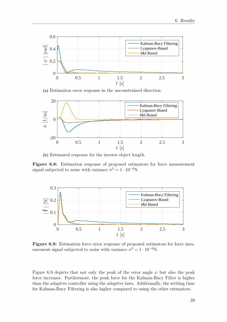
s . . . . . . . . . . . . . . . . . . . . . . . . . . . . . 386.8 Estimation response of proposed estimators for force measurement
signal subjected to noise with variance σ2 = 1 · 10−6N. . . . . . . . . 396.9 Estimation force error response of proposed estimators for force mea-
surement signal subjected to noise with variance σ2 = 1 · 10−6N. . . . 396.10 Estimation response of proposed estimators for initial estimation error
of the motion direction ψ(0) = 0.5rad. . . . . . . . . . . . . . . . . . 406.11 Estimation force error response of proposed estimators for initial es-
timation error of the motion direction ψ(0) = 0.5rad. . . . . . . . . . 41
xi

List of Figures
xii

List of Tables
4.1 Overview of the Estimators. . . . . . . . . . . . . . . . . . . . . . . . 27
6.1 Gains and parameters of the controllers and estimators. . . . . . . . . 316.2 Initial estimates. . . . . . . . . . . . . . . . . . . . . . . . . . . . . . 326.3 Standard values of the parameters. . . . . . . . . . . . . . . . . . . . 326.4 Values of the parameter with varying inverse object length simulation. 346.5 Values of the parameter with varying inverse object length simulation. 356.6 Values of the parameter with varying desired velocity. . . . . . . . . . 376.7 Values of the parameter with measurement signal noise. . . . . . . . . 386.8 Initial estimates. . . . . . . . . . . . . . . . . . . . . . . . . . . . . . 40
xiii

List of Tables
xiv

Acronyms
DOF degrees of freedom. 15
I&I Immersion and Invariance. v, ix, 3, 5, 9, 24, 25, 27, 31–33, 35–38, 41, 43
LLSME Linear Least Minimum Mean Square Estimator. 7
PI Proportional-Integral. v, 2, 19, 25, 30, 31
xv

Acronyms
xvi

1Introduction
The influence of service robotics has been increased over recent years [1]. An indica-tor for that is the growing trend towards using service robots not only for industrialpurposes, but also for personal and domestic usage. One crucial requirement for asuccessful manipulation of a number of tasks is to control the interaction between therobot and its environment. The best way to quantify the interaction is to measurethe interaction force at the end-effector, since high forces are undesirable in order toavoid damage to the structure of the robot and the manipulated environment. Theenvironment can consist of surfaces or objects, which possesses static or dynamicalproperties. In both cases, the permissible trajectory of the end-effector is restrictedby kinematic constraints.
po
pe
Figure 1.1: Object manipulation with pivoting dynamics.
There is a variety of possible interaction tasks. This thesis focuses on the manipula-tion of objects with pivoting dynamics, shown in Figure 1.1, since their manipulationenables to solve a wide range of problems within the service robotics field in domesticenvironment, for example opening doors. The scheme in Figure 1.1 shows an object,which possesses the aforementioned pivoting dynamics. More precisely, the objecthas one degree of freedom, so that it can only perform rotational motion aroundthe supporting point on the surface. Assuming that the object and its posture isunknown, implies that the position of the pivoting point is unknown. Within thisthesis a controller for a robot will be implemented to perform a manipulation taskfor unknown objects.
1

1. Introduction
1.1 Main research question
The objective of this thesis is to identify the relevant constraints of pivoting manip-ulation (Figure 1.1), and use them in an adaptive controller in order to achieve thefollowing manipulation task: rotating an unknown object around a pivot point bygrasping the object in a way that allows relative rotation between the gripper andthe object. In this case, two virtual revolute joints – one due to the pivot point onthe surface and one due to the non-fixed grasp – impose kinematic constraints onthe object. Since the object posture and its length is unknown, an adaptive con-troller has to be used to estimate these parameter uncertainties and to manipulatethe object. The research work will be applicable in performing service robots forexample to open unknown doors or turning a crank with a free knob.
1.2 Related Work
Since the topic of constrained manipulation is a common field of research in robotics,it is well-studied and lots of publications dealt with this topic. The books [2], [3] and[4] provide fundamental methods about modelling robot dynamics and kinematics inareas of unconstrained (non-contact) and constrained (interacted) manipulation. Es-pecially, the kinematic formulations in these books are important for the descriptionof the robot kinematics and its interaction with the environment. For this purpose,the interaction is modelled as geometric (kinematic) constraints. Furthermore, theaforementioned books give an overview of fundamental control techniques regardingmotion and force control. These control structures are also applied to regulate theinteraction of a robot with a dynamical environment assuming that the robot andthe environment are modelled as a rigid body system. Article [5] presents the mod-elling of kinematic constraints and describes an example in which a crank with a freeknob is turned. The manipulation of this crank possesses pivoting dynamics with apassive joint as is the case with the considered unknown object. Furthermore, arti-cle [6] analyses a camera navigation task on passive wrist-based robots and pivotingdynamics. Additionally, an adaptive PI-Cartesian position controller is presentedfor achieving the geometric modelled task of a laparoscopic assistant robot. Kine-matic constraints are frequently used for modelling the manipulation task, since itsimplifies the problem description. Article [7] analyses the manipulation with co-operating robots under uncertain kinematic parameters and presenting an adaptivecontroller which achieves parameter estimation during a desired object motion. Thearticles [8] and [9] cover the topic of opening doors under uncertainties with the aidof a velocity-controlled robot. The authors propose an adaptive controller whichestimates the unconstrained motion direction and the inverse length of a door. Theproposed adaptive laws - based on a Lyapunov function - are explained in this thesisand used for comparing the performance of different estimation methods, since adoor possesses dynamics with pivoting characteristics. Moreover, in [8] the gripperof the robot posses a fixed grasp such that the relative rotation velocity between theend-effector and the door is zero. Article [9] additionally considers also a gripperwith a non-fixed grasp which allows rotational velocity between the gripper and the
2

1. Introduction
unknown object. Both proposed velocity controllers rely on force measurements andestimate the unconstrained motion direction, rotational axis and the relevant size ofthe door.
Kalman-Bucy Filtering is the second used estimator in this thesis to estimate theunconstrained motion direction and object length during the manipulation task.Since Kalman Filtering is a widespread method to observe, smooth or filter signals,there is a vast literature with theory and background. Therefore, this thesis focuseson books [10] and [11] which present the theoretical background of different KalmanFilters and describes their function. Moreover, these books show how to design aKalman Filter for discrete or continuous systems.
The third used estimator is based on a relatively new design method for synthesisingthe adaptive laws. This framework is called Immersion and Invariance (I&I) andthe book [12] and its related articles, [13], [14] and [4] provide the relevant back-ground. The related literature cover not only the theory and methods synthesisingI&I based adaptive controllers but also general used designing methods (e.g. Lya-punov). Moreover, [12] provides examples of the different synthesising methods anddemonstrates the limits of the classical adaptive controllers.
1.3 MethodologyThe research work is organised as follows:
• System modelling with constraints description• Simulation environment development• Adaptive controller design• Scenario simulation• Performance evaluation
First of all the dynamical system containing the unknown object and manipulatorhave to be analysed. For this purpose the system is assumed to be a rigid multibodysystem. The model building phase is an important step, since both, the simulationmodel and the control method will be based on it. Furthermore, the simulationmodel has to be implemented on a simulation platform, e.g. MATLAB®/Simulink®,to run simulated experiments. Subsequently, an adaptive controller must be de-signed to estimate on-line the object length and the unconstrained motion direction,which are the uncertain parameters of the manipulated system. Furthermore, theperformance of the designed controller will be evaluated within the aforementionedsimulation environment.
1.4 Thesis OrganisationThis master thesis is organised with the following structure. First of all, Chapter2 provides the general mathematical notation and background knowledge on adap-
3

1. Introduction
tive control. Since the designed adaptive controller uses Kalman-Bucy Filtering,Lyapunov-based adaptive laws and I&I-based adaptive laws for estimating the un-known state and parameter, the background supplies the methods for synthesisingthese estimators. Chapter 3 describes the kinematic model of the unknown objectand the robot. Additionally, this chapter formulates the control objective for a suc-cessful task execution. Chapter 4, aims at developing the simulation environmentfor testing the designed controller and synthesising the adaptive controller whichincludes the control law and the estimators. The performance of the developedadaptive controller is evaluated within different simulation scenarios in Chapter 6.Finally, conclusions are drawn in Chapter 7.
4

2Background
This chapter gives an overview of the used notation followed by relevant theory ofadaptive control. Furthermore, Kalman-Bucy Filtering, Lyapunov-based and I&I-based adaptive controller are introduced for estimating parameters on-line.
2.1 Notation
The notation used in the thesis follows [15], [16] and [8] and is described in thefollowing.
Vectors and Matrices Small bold letters denote vectors and capital bold let-ters denote matrices. Additionally, ·, · and · denote vectors with unit magnitude,estimates and the error between the actual and the desired/estimated vector, re-spectively. The vectors
a(t) :=[ax(t) ay(t) az(t)
]>∈ R3,
b(t) :=[bx(t) by(t) bz(t)
]>∈ R3,
are used in the following paragraphs to introduce further notation. Furthermore,the time argument is often dropped out for notation convenience.
Projection Matrices A projection matrix projecting vectors along vector a isdefined as
P(a) = aa>
‖a‖2
and possesses the property P(a)> = P(a).
Matrix
P(a) = I3 −aa>
‖a‖2 ,
where I3 ∈ R3 denotes the identity matrix, projects vectors on a space consisting ofthe orthogonal complements of vector a and possesses the property P(a)> = P(a).
5

2. Background
Skew-Symmetric Tensor The skew-symmetric tensor
S(a) =
0 −az ayaz 0 −ax−ay ax 0
can be used for representing a cross product operation as follows
a × b = S(a)b.
Note that S(a)b = −S(b)a.
Rotation Matrix The orientation of a frame {I} with respect to the frame {J}is described by the rotation matrix IRJ ∈ R3. In case of {I} or {J} is identical tothe robot base frame {B}, the associated index will be omitted. A transformationfrom e.g. {J} to the base frame can be calculated as following
aI = RJJaI.
Note that a rotation matrix is orthogonal and the inverse transformation can bewritten as R−1 = R>.
Integral I(a(t)) denotes the element-wise time integration of the vector a(t) andis defined as
I(a(t)) =∫ t
t0a(τ) dτ.
2.2 Adaptive ControlThe performance of a conventional static control system is limited for dynamicalprocesses, which have uncertain system parameters. These parameters could be, forexample, unknown or time variant. Due to the dependency of the control law onthe system parameters, the controller performance can be improved by an adaptivecontrol structure which is shown in Figure 2.1.
Figure 2.1: Block diagram of a direct adaptive controller.
6

2. Background
Consider the dynamical system
x(t) = f (x(t), u(t),θ)y(t) = h (x(t), u(t),θ)
(2.1)
where x(t) ∈ Rn denotes the state vector, u(t) ∈ Rm the input vector, θ ∈ Rq
the parameter vector and y ∈ Rr the output vector. The plant in Figure 2.1 isrepresented by the dynamical system (2.1). Figure 2.1 shows also that the directadaptive control structure consists of a parameter estimator and a controller block.The former provides the on-line estimates of the system parameters, which are thearrays of the estimated parameter vector θ. Furthermore, the control law is designedfor the known parameter case, cf. [17]. There are many different methods to dealwith the on-line estimation. Since the performance of the adaptive controller highlydepends on the estimation quality, it is necessary to use suitable estimation methods.The following sections introduce the estimation methods used in the present thesis.
2.2.1 Kalman-Bucy FilterThe Kalman filter is a Linear Least Minimum Mean Square Estimator (LLSME) fora linear system, since it minimizes a quadratic function of estimation error, cf. [11].This type of filters is often used for filtering, prediction and smoothing of states, cf.[11]. The Kalman-Bucy filter is the continuous-time equivalent of the Kalman filter,which is formulated in discrete time. The following theory regarding the Kalmanand Kalman-Bucy filter is based on the books [11] and [10].
Consider the dynamical system
η(t) = F(t)η(t) + G(t)w(t)z(t) = H(t)η(t) + v(t)
(2.2)
where η(t) ∈ Rl and z(t) ∈ Rk denotes the state vector of a random process and themeasurement vector, respectively. F(t) ∈ Rl×l, G(t) ∈ Rl×w and H(t) ∈ Rk×l de-note the time-varying dynamic coefficient, process noise coupling and measurementsensitivity matrix, respectively. Furthermore, w(t) ∈ Rw and v(t) ∈ Rk are theuncorrelated process and observation noise process, respectively. To ensure that theestimated states η(t) converge to their actual values, the system (2.2) must be ob-servable. Furthermore, Q(t) ∈ Rl×l and R(t) ∈ Rk×k, which donates the covariancematrices of w(t) and v(t), are positive definite and are defined as
E〈w(t1)w>(t2)〉 = Q(t)δ(t2 − t1),E〈v(t1)v>(t2)〉 = R(t)δ(t2 − t1),
where E〈·〉 and δ(·) stands for the expectancy operator and the Dirac delta function,respectively. The update equation ˙η(t) for the state estimation is expressed as
˙η(t) = F(t)η(t) + K(t) (z(t)−H(t)η(t)) ,
7

2. Background
where K(t) ∈ Rl×k denotes the Kalman gain matrix and is defined as follows
K(t) = P(t)H>(t)R−1(t). (2.3)
The covariance matrix P(t) ∈ Rl×l in (2.3) are calculated with the aid of the fol-lowing Riccati differential equation
P(t) = F(t)P(t) + P(t)F>(t) + G(t)Q(t)G>(t)−P(t)H>(t)R−1(t)H(t)P(t).
The initial conditions for these estimated states and the covariance matrix is definedas
η(0) := η0
P(0) := P0.
2.2.2 Lyapunov-Based Adaptive LawConsider the dynamic system (2.1). As aforementioned, the adaptive control schemeincludes the controller and the on-line parameter estimation component, which com-prises the control law u(x,θ) for the known parameters and the update law
˙θ = w
(x, θ
).
Lyapunov functions are often used for analysing the stability of nonlinear systems.The direct Lyapunov method is also applicable for synthesising adaptive laws. Inparticular the problem of designing an adaptive controller is formulated as stabilityproblem.
Theorem 2.2.1 (Lyapunov Function). V (x,θ) ∈ R is said to be a Lyapunov func-tion of the system (2.1) if
V (x,θ) > 0 in D \ {0} (2.4)V (x,θ) ≤ 0 in D
is satisfied, where V (x,θ) ∈ R and D = {x ⊆ Rn,θ ⊆ Rq} denotes the deriva-tive with respect to time of the Lyapunov function and the domain, respectively.Additionally, V (x,θ) has to be a continuously differentiable function, c.f. [18].
For further reading, Khalil [18] provides more details on the Lyapunov theory.
Assumption 2.1. There exists a Lyapunov function V (x,θ) so that the update law˙θ cancels the unknown parameter terms in V (x,θ) and renders V (x,θ) negativesemi-definite, c.f. [12].
The first step is to find a Lyapunov function candidate, which satisfies the require-ment (2.4) of the Theorem 2.2.1. Furthermore, the update law ˙
θ has to be chosenin such a way so that V (x,θ) is independent of the unknown parameters.
8
2. Background
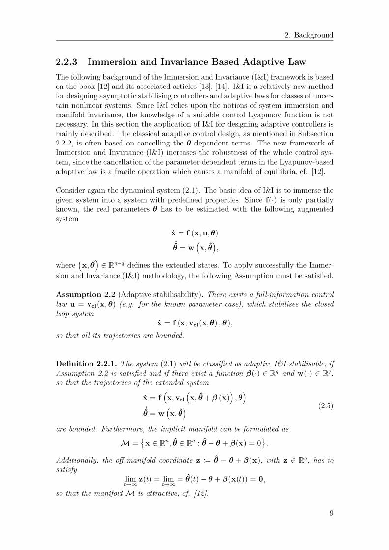
2.2.3 Immersion and Invariance Based Adaptive LawThe following background of the Immersion and Invariance (I&I) framework is basedon the book [12] and its associated articles [13], [14]. I&I is a relatively new methodfor designing asymptotic stabilising controllers and adaptive laws for classes of uncer-tain nonlinear systems. Since I&I relies upon the notions of system immersion andmanifold invariance, the knowledge of a suitable control Lyapunov function is notnecessary. In this section the application of I&I for designing adaptive controllers ismainly described. The classical adaptive control design, as mentioned in Subsection2.2.2, is often based on cancelling the θ dependent terms. The new framework ofImmersion and Invariance (I&I) increases the robustness of the whole control sys-tem, since the cancellation of the parameter dependent terms in the Lyapunov-basedadaptive law is a fragile operation which causes a manifold of equilibria, cf. [12].
Consider again the dynamical system (2.1). The basic idea of I&I is to immerse thegiven system into a system with predefined properties. Since f(·) is only partiallyknown, the real parameters θ has to be estimated with the following augmentedsystem
x = f (x,u,θ)˙θ = w
(x, θ
),
where(x, θ
)∈ Rn+q defines the extended states. To apply successfully the Immer-
sion and Invariance (I&I) methodology, the following Assumption must be satisfied.
Assumption 2.2 (Adaptive stabilisability). There exists a full-information controllaw u = vcl(x,θ) (e.g. for the known parameter case), which stabilises the closedloop system
x = f (x, vcl(x,θ) ,θ),so that all its trajectories are bounded.
Definition 2.2.1. The system (2.1) will be classified as adaptive I&I stabilisable, ifAssumption 2.2 is satisfied and if there exist a function β(·) ∈ Rq and w(·) ∈ Rq,so that the trajectories of the extended system
x = f(x,vcl
(x, θ + β (x)
),θ)
˙θ = w
(x, θ
) (2.5)
are bounded. Furthermore, the implicit manifold can be formulated as
M ={x ∈ Rn, θ ∈ Rq : θ − θ + β(x) = 0
}.
Additionally, the off-manifold coordinate z := θ − θ + β(x), with z ∈ Rq, has tosatisfy
limt→∞
z(t) = limt→∞
= θ(t)− θ + β(x(t)) = 0,
so that the manifoldM is attractive, cf. [12].
9

2. Background
More precisely, Definition 2.2.1 means that the trajectories of x and θ asymptoti-cally converges to the manifold M and remains there. Additionally, the unknownparameter vector θ is replaced by the expression θ+β(x), such that the parameterestimation is not directly applied to the extended system (2.5).
10

3System and Problem Description
Section 3.1 elaborates on the manipulation task and the interaction between themanipulator, which is considered to be a robot, and the unknown object. After thatthe kinematics of the manipulator are analysed and it is defined how the controlsignal affects the end-effector velocity of the robot. Finally, Section 3.3 provides adetailed description of the control problem by introducing the control objective.
3.1 Task KinematicsIn this section, the kinematic constraints involved in the manipulation task arederived. The robot and the unknown object can be considered as a rigid bodysystem in which the end-effector is connected with the object by a passive joint.
zb
yb
xb
{B}
zw
yw
xw
{W}
zs
ys
xs
{S}
pb
ps
po
xe
zeye
{E}
pe
r
Figure 3.1: Coordinate system transformation of the frames World{W}, Base{B},Supporting Point{S} and End-effector{E}.
Figure 3.1 shows an example for a possible constellation of the frames. The redvectors denote the translational relation between the used frames. The world frame{W} is a stationary reference coordinate system, which is the origin of a robot sys-tem. Furthermore, all other frames are related to {W}. The base coordinate system{B}, which is located at a robot’s base, is the reference frame of the robot. Fur-thermore, the end-effector frame {E} represents the position and orientation of theend-effector, which is mounted at the Tool Centre Point (TCP) of the manipulator.The supporting point frame {S} is located at the contact point between the surface
11

3. System and Problem Description
and the unknown object and is therefore the centre of the rotational motion of theobject. The unit vector zs ∈ R3 is normal to the surface, while xs ∈ R3, ys ∈ R3 canbe arbitrarily chosen. {H} denotes the handle frame which represents the positionand orientation of the moveable end of the unknown object. The origin of the handle{H} and the end-effector frame {E} are located at the same position. This impliesthe following constraint for the position of the end-effector:
pe − ph ≡ 0,
where pe ∈ R3 and ph ∈ R3 denotes the position vector of the end-effector {E} andhandle frame {H}, respectively.
Assumption 3.1. There exists no relative translation between the end-effector andhandle frame,
hpe ≡ 0.
Assumption 3.2 (Planar Motion). The motion of the unknown object is assumedto be planar. Therefore, the object can only afford one degree of freedom motion.Additionally, the rotation axis zh ∈ R3 can be arbitrary and it is not necessary thatzh ∈ R3 and zb ∈ R3 are parallel.
Regarding Assumption 3.2, the orientation of {H} can be defined based on therotational axis zh ∈ R3 and the position of the unknown object and consequentlyon the constraints of the manipulation task. The vector yh ∈ R3 is unit and pointstowards the origin of the supporting point frame {S}. Since Cartesian right-handcoordinate systems are used, the unconstrained motion direction xh ∈ R3 can beformulated as
xh = S(yh
)zh.
Figure 3.2 depicts an alternative parametrisation of the handle frame vectors, whichincludes the rotation angle ϕ ∈ R of the unknown object. The following vectors xh,yh and zh describe the orientation of the handle frame {H} with respect to the baseframe {B}
xh = Rs
cosϕ0
sinϕ
, yh = Rs
− sinϕ0
cosϕ
, zh = Rs
010
, (3.1)
where Rs ∈ R3 is the rotation matrix between the base {B} and surface frame {S}.
Assumption 3.3 (Object Grasp). The end-effector grasps the unknown object in away that allows relative rotation between the end-effector and the object. Hence, thegrasping point is considered as a passive joint.
Due to Assumption 3.3, the orientation of {H} with respect to the end-effector
12

3. System and Problem Description
Figure 3.2: Angle parametrisation.
frame {E} and therefore the rotation matrix eRh ∈ R3 can be time-varying.
The radial vector r ∈ R3 represents the unknown object and connects the origins ofthe frames {H} and {S}. Since the origins of {E} and {H} are identical, r connectsalso the origins of the frames {E} and {S}. Vector r can be defined based on poand ph or pe as follows:
r := po − ph = po − pe (3.2)The radial vector r is always parallel to yh, therefore
r = 1κ
yh. (3.3)
is an alternative description for r, where κ ∈ R+0 denotes the inverse length of
the object line. Figure 3.3 depicts an example object including the object line,which always connects the end-effector and the contact point between the objectand surface. Additionally, κ describes the curvature of the end-effector trajectory.By differentiating equation (3.2), the velocity r of the unknown object is as follows:
r = po − ph = Rhhr + Rh
hr= Rh
hr = RhRhT r
= S(ωh)r = −S(r)ωh,
(3.4)
where ωh ∈ R3 denotes the rotational velocity of the handle frame {H}. The handleframe {H} is a body-fixed coordinate system of the unknown object, the rotationalvelocity of the unknown object ω ∈ R3 can be expressed as
ω ≡ ωh.
The rotational axis of the object and zh are parallel, therefore an alternative ex-pression of the rotational velocity vector is
ωh = ωzh, (3.5)
13

3. System and Problem Description
Figure 3.3: Example object.
where ω denotes the magnitude of the rotational velocity. Since the end-effector{E} and handle frame {H} has the same origin, the end-effector velocity v ∈ R3
can be expressed with the aid of (3.4) as
v = −r = S(r)ω. (3.6)
During this manipulation task, the dynamics of the interaction between the robotand its environment is restricted by kinematic constraints. In other words, the mo-tion of the manipulated object is constrained, which causes forces, by moving alongthe constrained direction, cf. [2]. Since the end-effector trajectory is constrained bythe object, the unconstrained motion direction is perpendicular to the radial vectorr. Because of the planar motion, xh is the motion direction by definition. Fromthis it follows that the end-effector velocity v can be parametrized as following
v = vxh, (3.7)
where v ∈ R denotes the velocity magnitude of the end-effector.
Projecting the end-effector velocity v along xh gives the scalar value
v = xh>v (3.8)
of the end-effector velocity. Furthermore, equation (3.7) implies that the constrainedtranslational velocity of the end-effector is
P(xh)v = 0.
Additionally, Equations (3.3),(3.5),(3.6) and (3.7) give the following relation betweenthe translational and rotational velocities
v = ω
κ(3.9)
14
3. System and Problem Description
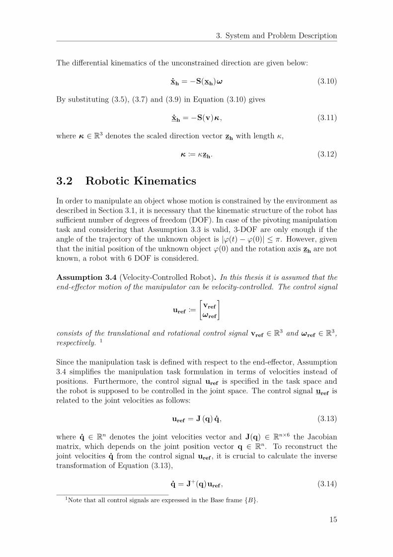
The differential kinematics of the unconstrained direction are given below:
xh = −S(xh)ω (3.10)
By substituting (3.5), (3.7) and (3.9) in Equation (3.10) gives
xh = −S(v)κ, (3.11)
where κ ∈ R3 denotes the scaled direction vector zh with length κ,
κ := κzh. (3.12)
3.2 Robotic KinematicsIn order to manipulate an object whose motion is constrained by the environment asdescribed in Section 3.1, it is necessary that the kinematic structure of the robot hassufficient number of degrees of freedom (DOF). In case of the pivoting manipulationtask and considering that Assumption 3.3 is valid, 3-DOF are only enough if theangle of the trajectory of the unknown object is |ϕ(t)− ϕ(0)| ≤ π. However, giventhat the initial position of the unknown object ϕ(0) and the rotation axis zh are notknown, a robot with 6 DOF is considered.
Assumption 3.4 (Velocity-Controlled Robot). In this thesis it is assumed that theend-effector motion of the manipulator can be velocity-controlled. The control signal
uref :=[vrefωref
]
consists of the translational and rotational control signal vref ∈ R3 and ωref ∈ R3,respectively. 1
Since the manipulation task is defined with respect to the end-effector, Assumption3.4 simplifies the manipulation task formulation in terms of velocities instead ofpositions. Furthermore, the control signal uref is specified in the task space andthe robot is supposed to be controlled in the joint space. The control signal uref isrelated to the joint velocities as follows:
uref = J (q) q, (3.13)
where q ∈ Rn denotes the joint velocities vector and J(q) ∈ Rn×6 the Jacobianmatrix, which depends on the joint position vector q ∈ Rn. To reconstruct thejoint velocities q from the control signal uref , it is crucial to calculate the inversetransformation of Equation (3.13),
q = J+(q)uref , (3.14)1Note that all control signals are expressed in the Base frame {B}.
15

3. System and Problem Description
where J+(q) = J(q)>[J(q)J(q)>
]−1∈ R6×n denotes the pseudo inverse matrix of
J(q), cf. [19]. Depending on the number of robot joints, the Jacobian matrix canbe not square and therefore the real inverse matrix does not exist.
A manipulator can be mechanically represented as a kinematic chain of multi rigidbodies, cf. [2] The kinematic structure of a robot is nearly always driven by anelectrical actuator, which generates torque and thus accelerates the joints. There-fore, a motion controller is required for regulating the joint velocities q and thusthe end-effector velocity v.
Assumption 3.5 (Ideal Motion Controller). The inner motion control loop of therobot is sufficiently fast and includes a force and torque compensation, so that thejoint velocity errors ˙q ∈ Rn between the desired and real value is negligible,
˙q := q − qd ≈ 0.
Assumption 3.5 and Equation (3.14) implies that not only the error of the jointvelocities ˙q but also the error of the end-effector velocity:
v := v − vref ≈ 0 (3.15)ω := ω − ωref ≈ 0
are negligible, where v ∈ R3 and ω ∈ R3. Furthermore, if Assumption 3.5 is valid,the object mass and inertia will have a strong influence on the force signal, which isgenerated by the wrist-mounted force sensors. Additionally, in order to reduce therisk of injuring humans in the domestic environment, the following Assumption hasto be considered.
Assumption 3.6 (Object Mass and Inertia). The commanded velocity signals urefof the end-effector and therefore, the unknown object is adequately low, such that theinfluence of object dynamics on the force measurement is negligible.
3.3 Control ObjectiveFigure 3.4 shows the relevant parts and the interaction of the overall system. The fol-lowing control objective is based on the article [9], that considers a similar manipula-tion task - opening a unknown door. First of all the interaction force finteraction ∈ R3
between the unknown object and the robot has to be regulated. Consider the desiredinteraction force fd ∈ R3, one goal is to adjust the control signal uref , so that the in-teraction force converges to the desired force fd. The interaction force objective canbe satisfied by projecting the desired force along the constrained motion direction.The following equation describes the aforementioned first control objective,
P (xh)f → P (xh)fd.
16

3. System and Problem Description
Figure 3.4: Block diagram of the total system, c.f. [9].
The second objective of the designed controller is to move the object, with a desiredvelocity vd ∈ R, on circular trajectory around the supporting point. Consider thatthe unconstrained motion direction is expressed in the object fixed handle frame{H},
vd = vdxh, (3.16)
where vd ∈ R3 denotes the desired velocity vector of the end-effector. The secondcontrol objective is therefore,
v → vd
Due to the fact that the orientation and length of the object is not known, theorientation and its differential kinematics have to be estimated in the end-effector{E} or robot base frame {B}. Consider the vector κ from Equation (3.12) whichconsists of the information of the rotation axis and the inverse length of the objectand therefore combines two unknown parameters in one vector.
Assumption 3.7 (Known Rotation Axis). The rotation axis zh of the handle frame{H} is known.
Assumption 3.8 (Unknown Rotation Axis). The rotation axis zh of the handleframe {H} is unknown.
Depending which one of the following Assumption is satisfied, the control problem,especially the dimension of the estimation problem, changes.
17

3. System and Problem Description
18

4Controller Design
This chapter describes the control law and design of the different estimation al-gorithms. Since the overall performance of the manipulation task depends on thecontroller design, this part is an essential part of this master thesis.
4.1 Control LawLet xh ∈ R3 denote the estimate of the unconstrained motion direction. Since therobot is velocity controlled (Assumption 3.4), the output of the designed controlleris the signal uref . It is not necessary to control the rotational velocity of the end-effector, since the robot grasps the unknown object in a non-fixed way (Assumption3.3). An additional rotational controller is only required for avoiding collisionsbetween the unknown object and the end-effector or optimising the position of therobot joints. Therefore, the control signal uref depends mainly on the translationalvelocity control signal vref . As described in Section 3.3, the control law can bedivided into two orthogonal terms. The first term is a feed-forward term controllingthe motion along the unconstrained xh and the second term is the term whichcontrols the force along the constrained motion direction P (xh). Consider thefollowing control law
vref = vdxh − P(xh)vf (4.1)which consists of the aforementioned orthogonal terms, c.f. [9]. Since xh is notknown, the control law (4.1) depends on the estimated unconstrained direction xh.Ideally, xh should have a unit magnitude, since it denotes a direction vector. If‖xh‖ = 1 the velocity of the end-effector v converge to the desired velocity vd. Thegain of the estimated motion direction vd represents the desired velocity term of thecontrol law, based on Equation (3.16). The second term of the control law (4.1),along the constrained direction, constructs the force controller. The vector vf ∈ R3
denotes the PI force feedback input with
vf = αf f + βfI[P(xh) f
], (4.2)
where αf , βf ∈ R are positive control gains and
f := f − fd
denotes the force error, c.f. [9]. The force control term (4.2) compensates thekinematic uncertainties of the unknown object during the manipulation task. Addi-tionally, term (4.2) also compensates partially the error between the estimated andreal motion direction, xh and xh respectively.
19

4. Controller Design
4.2 On-Line Estimator DesignAs mentioned in Section 2.2, the direct adaptive control structure contains a con-troller and an on-line parameter estimation component. The following describes thedetails of designing different on-line parameter estimators, that estimate the un-known parameters xh and κ. This parameter estimation adapts the control law inSubsection 4.1, since it uses these parameters for calculating the reference velocityof the end-effector.
In order to design an on-line estimator for the unknown parameters, the estimationerrors have to be defined. In this regard, κ ∈ R3 denotes the error of the scaledrotation axis and is given by
κ(t) = κ(t)− κ. (4.3)
Since κ is constant, the derivative of estimation error of the inverse object lengthvector has the following form
˙κ = ˙κ. (4.4)The second estimation error is ψ(t) ∈ R which defines the angular error of themotion direction. More precisely, it denotes the angle between the unknown xh andestimated unconstrained direction xh. Since both directions are unit vectors, theinner product can be formulated as
cosψ(t) = xh>(t) xh(t). (4.5)
To get the relationship between the derivative of the error angle ψ(t) and the deriva-tive of the estimated unknown direction, both sides of Equation (4.5) has to bedifferentiated as follows:
ddt(
cosψ(t))
= ddt((xh
>xh
)= xh
>xh + xh> ˙xh
= (−S(v)κ)> xh + xh> ˙xh
= −v>S(κ)xh + xh> ˙xh
= xh>(
˙xh − vS(κ)xh
)⇔ −ψ(t) sinψ(t) = xh
>(
˙xh − vS(κ)xh
)(4.6)
The differentiation of (4.5) reveals that the error angle ψ(t) depends on the esti-mation rate and the object motion velocity, c.f. [9]. The velocity error v can beexpanded into one term along xh and one term along its orthogonal complementspace. Substituting the object velocity (3.7) and control law (4.1) in the velocityerror formulation (3.15) leads to
v = vxh − vdxh + P(xh)vf
= P (xh) v + P (xh) v − vdxh + P(xh)vf
= v cosψ xh + P (xh) v − vdxh + P(xh)vf
= P (xh) (v + vf ) + (v cosψ − vd) xh.
20

4. Controller Design
Assumption 3.5 and the resulting negligible velocity error implies the followingclosed-loop relations
P (xh) vf = −vP (xh) xh (4.7)
v = vdcosψ (4.8)
Taking the norm of the term along the complement space of xh gives
‖P (xh) vf‖ = |vd tanψ|. (4.9)
For example 4.9 shows, how the estimation error ψ affects the force errors and theend-effector velocity error. Additionally, the closed-loop Equations (4.7), (4.8) and(4.9) give the evidence that the higher the unconstrained direction error ψ is, thehigher the force on the object can be, c.f. [9].
4.2.1 Kalman Filter with Known Rotation AxisIf Assumption 3.7 (Known Rotation Axis) is satisfied, the linear parameter systemwill possess the following form
θ(t) = F(t) θ(t)z(t) = H(t) θ(t),
(4.10)
where θ(t) =[xh>(t) κ
]>∈ R4 is the parameter vector, which consists of the
unknown parameters and F(t) ∈ R4×4
F(t) =[0 −S(v(t))zh0 0
]denotes the time-varying dynamic coefficient matrix. Its first row is based on theEquation (3.11) and since the object length is constant, κ is not varying. Onepossible measurement is the velocity of the end-effector, which is captured in themeasurement vector z(t) ∈ R3. From this it follows, that the measurement sensitiv-ity matrix H(t) ∈ R3×4 can be formulated as
H(t) =[v(t)I3 0
].
Since the robot is velocity-controlled the matrices F(t) and H(t) can be expressedin terms of the reference velocity,
F(t) =[0 −S(vref (t))zh0 0
]H(t) =
[vref (t)I3 0
].
Equation (3.8) and (3.15) shows that vref depends on the unknown state xh. Usingthe expression
vref (t) = ‖vref (t)‖ sgn(xh>(t) vref (t)
)(4.11)
21

4. Controller Design
it is possible to calculate vref without the knowledge of the motion direction forxh>xh > 0, c.f. [9].
The update equation for the parameter estimation with known rotation axis is de-fined as
˙θ = F(t)θ(t) + K(t)
(z(t)−H(t)θ(t)
),
where θ(t) =[xh>(t) κ(t)
]>denotes the estimated parameter vector. Furthermore,
the Kalman gain matrix K(t) ∈ R4 can be calculated with the following equations,
K(t) = P(t)H>(t)R−1,
where R(t) ∈ R3×3 denotes the covariance matrix of the measurement noise. Thecovariance matrix P(t) ∈ R4×4 is calculated with the aid of the Riccati differentialequation
P(t) = F(t)P(t) + P(t)F>(t) + G(t)Q(t)G>(t)−P(t)H>(t)R−1(t)H(t)P(t),
where Q ∈ R3 denotes the covariance matrix of the plant noise. The initial condi-tions for this Kalman filter are
θ(0) = θ0,
P(0) = P0.
4.2.2 Kalman Filter with Unknown Rotation AxisIn case of unknown rotation axis, Assumption 3.8 is satisfied, the parameter systemhas the same form as (4.10). Consider the parameter vector θ(t) =
[xh>(t) κ>
]∈
R6. The scaled rotation axis vector κ consists of the inverted length κ and therotation axis zh, as mentioned in (3.12). Since the time-varying dynamic coefficientmatrix F(t) ∈ R6×6
F =[0 −S (v(t))0 0
]does not include the information of the rotation axis zh, the parameter systemdimension increases to six. In this case the measurement sensitivity matrix H(t) ∈R3×6 has the following form,
H =[v(t)I3 0
].
The Kalman gain matrix K(t) ∈ R6×3 and Riccati differential equation have thesame form as in the known rotation axis case, only the dimension is different.
4.2.3 Lyapunov-Based Adaptive LawThe following design of the adaptive laws are based on the Article [9]. As describedin the background, Section 2.2.2, the first step of the Lyapunov-based adaptive lawdesign is to find an appropriate Lyapunov function candidate V , which depends on
22

4. Controller Design
the unknown motion direction xh and the scaled rotation axis vector κ. Considerthe estimation error definition (4.5) of the unconstrained direction and (4.3) of thescaled object length vector.
Consider the Lyapunov function candidate
V = 1− cosψ + 12 κ>Γκκ
which is positive definite for the domain D = {ψ ∈ R, κ ∈ R3 : |ψ| < π2}, cf. [9]. In
order to satisfy Theorem 2.2.1 and to synthesise the adaptive laws, we calculate thederivative of the Lyapunov function V (ψ, κ):
V = ψ sinψ + κ>Γκ˙κ,
where Γκ ∈ R3×3 denotes a positive definite gain matrix. Substituting (4.3), (4.4)and (4.6) in V leads to the following derivation:
V = −xh>(
˙xh − vS(κ− κ)xh
)+ κ>Γκ
˙κ
= −xh>(
˙xh − vS(κ)xh + vS(κ)xh
)+ κ>Γκ
˙κ
= −xh>(
˙xh + vS(xh)κ)− vxh
>S(κ)xh + κ>Γκ˙κ
= −xh>(
˙xh + vS(xh)κ)− vκ>S(xh)xh + κ>Γκ
˙κ
= −xh>(
˙xh + vS(xh)κ)− κ>
(vS(xh)xh − Γκ
˙κ)
= −xh>(
˙xh + vS(xh)κ)− κ>
(S(xh)v − Γκ
˙κ)
(4.12)
According to Theorem 2.2.1, the next step is to select the adaptive laws such thatV is negative semi-definite and the unknown parameters are cancelled. The article[9] proposes the following update law for xh
˙xh = −vref S(xh)κ − γvref P(xh)vf , (4.13)
where γ ∈ R+ is a positive constant control gain for tuning the update rate. Dueto Assumption 3.4 (Velocity-Controlled Robot) is valid, the scalar velocity of theend-effector v can be substituted by the scalar reference velocity vref . The first termupdate law (4.13) cancels the unknown parameters in (4.12) for sufficient high γ.Since the unconstrained direction xh is time varying, the second term is necessaryto ensure the convergence of xh to the unknown motion direction xh. The updatelaw for xh depends on the estimation of the estimated scaled rotation axis κ, whichcan be on-line estimated by the update law
˙κ = ΓκS(xh)vref . (4.14)
Projecting (4.7) along the motion direction xh and substituting (4.5) yields
xh>P(xh)vf = −vxh
>P(xh)xh
= −vxh>(I3 − xhxh
>)
xh
= −v(1− cos2 ψ) = −v sin2 ψ.
(4.15)
23

4. Controller Design
Due to the manipulator is velocity-controlled, v can be substituted by vref in (4.15).Substituting the update laws (4.13) and (4.14) shows that V is negative semi-definitedue to the cancelled terms and equation (4.15). Therefore, V satisfies the Theorem2.2.1. Additionally, vref can be calculated in the same way as in (4.11).
The control law (4.1) suggests that the estimated motion direction vector xh mustbe unit in order to achieve the desired control objective. The update law ˙xh ensuresthat the norm of the unconstrained direction vector xh(t) is invariant. Projecting˙xh along the xh yields
xh> ˙xh = −vref xh
>S(xh)κ− γvref xh>P(xh)vf
⇔ ddt
(12‖xh‖2
)= −vrefκ
>S(xh)xh − γvref xh>(I3 − xhxh
>)
vf
= −vrefκ>S(xh)xh − γvref
(xh> − xh
>xhxh>)
vf = 0
From this it follows that ‖xh(0)‖ = ‖xh(t)‖, ∀t ≥ 0 and therefore, if the initialvalue of the estimated motion direction is ‖xh(0)‖ = 1 the magnitude will be unitat all time.
The article [9] provides more details on the stability analysis and the convergenceof the estimated parameters.
4.2.4 Adaptive Law Design via Immersion and InvarianceConsidering the alternative parametrisation (3.1) of the handle frame {H} whichdepends on the scalar parameter ϕ and Assumption 3.7 is satisfied. Therefore, theestimation problem consists of two scalar parameters, the angle ϕ and the invertedobject length κ. Additionally, for this case the second column of the rotation matrixRs is known and the rotation axis zh can be calculated. Since the following problemformulation is based on the angle error ψ and its dynamics ψ, the rotational velocityof the object can be parametrised as
ϕ = −vκ.
Furthermore, the aforementioned angle error ψ is defined in this case as
ψ := ϕ− ϕ. (4.16)
The derivative of (4.16) yields to the first-order differential equation, which is partof the augmented system
ψ = ˙ϕ+ vκ
˙κ = w,(4.17)
where w ∈ R denotes the update law and define in the extended space (ψ, κ) ∈ R2
the implicit manifold
M = {ψ ∈ R, κ ∈ R : κ− κ+ β(ψ) = 0} .
24

4. Controller Design
The dynamics of the augmented system (4.17) is restricted by the manifoldM∈ R.The invariance property of the manifoldM is described by the equation
ψ = ˙ϕ+ v (κ+ β(ψ)) .
The update law for ϕ can be analogous designed for the known rotation axis withthe angle parametrisation case as for the unknown rotation axis (4.13). In particularthe update law is proposed as follows:
˙ϕ = −γvdvf − v (κ+ β(ψ)) , (4.18)
where γ ∈ R+ denotes the update rate gain. Furthermore, vf denotes the scalarexpression of the PI-force controller of the control law (4.1) and is defined as
vf = yh>vf ,
where yh is the estimated constrained direction (3.1). The next step of the I&Imethod is to select an update law for κ which renders the manifold M invariant.Consider the off-manifold z is given by
z := κ− κ+ β(ψ). (4.19)
The following off-manifold dynamics z, which is given by the time derivative of(4.19), must be asymptotic stable.
z = ˙κ+ ∂β(ψ)∂ψ
ψ (4.20)
= ˙κ+ ∂β(ψ)∂ψ
[ ˙ϕ+ v (κ+ β(ψ)− z)]
In the next step the update law ˙κ has to be chosen in such a way so that the manifoldM is invariant:
˙κ = −∂β(ψ)∂ψ
[ ˙ϕ+ v (κ+ β(ψ))]
(4.21)
Substituting the update law for κ (4.21) in the off-manifold dynamics (4.20) yields
z = −∂β(ψ)∂ψ
z. (4.22)
Consider the Lyapunov function candidate V in order to analyse the stability prop-erties of the off-manifold dynamics (4.22) by the direct Lyapunov method.
V = 12z
2 (4.23)
The Lyapunov function candidate V in (4.23) is positive definite for all z ∈ R\{0}.
V (z) = zz = −∂β (θ)∂θ
z2 (4.24)
25
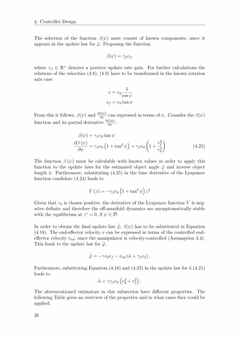
4. Controller Design
The selection of the function β(ψ) must consist of known components, since itappears in the update law for ϕ. Proposing the function
β(ψ) = γβvf ,
where γβ ∈ R+ denotes a positive update rate gain. For further calculations therelations of the velocities (4.8), (4.9) have to be transformed in the known rotationaxis case:
v = vd1
cosψvf = vd tanψ
From this it follows, β(ψ) and ∂β(ψ)∂ψ
can expressed in terms of ψ. Consider the β(ψ)function and its partial derivative ∂β(ψ)
∂ψ:
β(ψ) = γβvd tanψ∂β (ψ)∂ψ
= γβvd(1 + tan2 ψ
)= γβvd
(1 +
v2f
v2d
)(4.25)
The function β (ψ) must be calculable with known values in order to apply thisfunction to the update laws for the estimated object angle ϕ and inverse objectlength κ. Furthermore, substituting (4.25) in the time derivative of the Lyapunovfunction candidate (4.24) leads to
V (z) = −γβvd(1 + tan2 ψ
)z2
Given that vd is chosen positive, the derivative of the Lyapunov function V is neg-ative definite and therefore the off-manifold dynamics are asymptomatically stablewith the equilibrium at z∗ = 0, if ψ ∈ D.
In order to obtain the final update law ˙ϕ, β(ψ) has to be substituted in Equation(4.18). The end-effector velocity v can be expressed in terms of the controlled end-effector velocity vref , since the manipulator is velocity-controlled (Assumption 3.4).This leads to the update law for ϕ,
˙ϕ = −γvdvf − vref (κ+ γβvf ) .
Furthermore, substituting Equation (4.18) and (4.25) in the update law for κ (4.21)leads to
˙κ = γγβvf(v2d + v2
f
).
The aforementioned estimators in this subsection have different properties. Thefollowing Table gives an overview of the properties and in what cases they could beapplied:
26

4. Controller Design
Estimation Kalman-Bucy Filter Lyapunov-Based I&I-BasedUnconstrainedMotion Direction X X X
Object Line X X XRotation Axis X X
Table 4.1: Overview of the Estimators.
Table 4.1 shows that the I&I-based estimator is only applicable for objects withknown rotation axis.
27

4. Controller Design
28

5Simulation Model
In order to evaluate the performance of the designed adaptive controller, it is neces-sary to create a testing platform. This could be in this case a simulation model or aphysical experiment. It is advisable to indicate the generality of the controller withina simulation model, since the tests of different simulation scenarios can be imple-mented in a short time. Additionally, the risk of damaging the experiment hardwarecan be reduced by testing the approach first in simulation. Since a simulation modelis often an approximation of a real experiment setup, it is recommended to evaluatethe performance of the adaptive controller in further experiments. In the follow-ing sections the used modelling method of the mechanical system and end-effectoractuation is introduced.
5.1 Object-orientated Physical Modelling
As Albert Einstein said: "Everything should be made as simple as possible, butnot simpler." This axiom could be applied for the simulation model which shouldbe as simple as possible. In order to depict all relevant dynamics the simulationmodel should also be as close to the reality as necessary. Since the task kinematicsin Section 3.1 is described by the constraints and the object inertia is assumed tobe negligible (Assumption 3.6), it is reasonable to utilise a software platform forobject-orientated physical modelling. With this modelling method it is not neces-sary to identify all dynamical equations of the system. The simulation environmentSimMechanics™ Second Generation is used for modelling the mechanical structureof the systems, which is included in the SimScape™ toolbox. The considered rigidbody system can be modelled by using blocks representing body elements, joints,frames and sensors in Simulink®, cf. [20].
Figure 5.1 depicts the modelling of the task kinematic which consists of the in-teraction dynamics of the unknown object and the surface. This object-orientatedphysical model contains body elements and joints which are linked by physical con-nections. As described in Assumtion 3.2 the unknown object can rotate around thepivoting point on the surface. This constraint is represented by a revolute jointwhich also measures the angle, angular velocity and force between the unknown ob-ject and the surface. The passive joint, which is shown in Figure 5.1, represents thelose grasp of the unknown object by the robot end-effector. An additional advantageto use SimMechanics™ is that this toolbox provides an included animation frame-work. This animation gives users a visual feedback of the simulation and shows the
29

5. Simulation Model
simulation results without any additional implementation.
Figure 5.1: Cut-out from the Simulink® model of the task kinematics.
5.2 Velocity ControllerDuring the manipulation task, the robot end-effector must be able to move theobject with a desired velocity. Since the SimMechanics™toolbox does not supportvelocity commanded actuation, the end-effector is actuated by forces. Calculatingthe desired forces with feed forward terms cause errors for objects with differentgeometries or masses, therefore a velocity PI-controller is applied to regulate theforce fe ∈ R3 on the end-effector. This PI-controller has the following form
fe = αv ve + βvI[ve],
where αv, βv ∈ R are positive controller gains and
ve := vref − ve
denotes the velocity error of the end-effector between the controlled velocity vrefand the end-effector velocity ve ∈ R3.
30

6Results
This chapter contains the development of the simulation scenarios, in order to eval-uate the performance of the designed estimators Kalman-Bucy Filtering with un-known rotation axis, Lyapunov-based adaptive laws and Immersion and Invariance-based adaptive laws. Furthermore, different scenarios are presented for the purposeto make inferences regarding the robustness of the adaptive controller. The simula-tion results base on the simulation model in Chapter 5.
6.1 Simulation Results
The following scenarios cover different object lengths, different desired velocitiesalong the motion direction and the impact of the noise in the force sensor signal f.With the aid of these scenarios, it is possible to demonstrate the robustness of thedifferent estimation methods and reveal their strengths and weaknesses.
Parameter ValueVelocity αv 25controller βv 2Force αf 5 · 10−2
Controller βf 5 · 10−3
P(0) 1 · 105I6Kalman-Bucy R 1 · 10−4I3
Filter Q 1 · 10−5
G[1 1 1 1 1 1
]>Lyapunov γ 2 · 104
Γκ 2 · 104I3I&I γ 5 · 103
γβ 1 · 104
Table 6.1: Gains and parameters of the controllers and estimators.
The chosen parameters of the velocity PI-controller in the simulation model and theforce PI-controller in the control law are displayed in Table 6.1 and are same forevery scenario. Additionally, the initial values for the inverse object length and themotion direction offset are presented in the following Table.
31

6. Results
Parameter Initial Value Unitκ(0) 7 m−1
ψ(0) 0.2 rad
Table 6.2: Initial estimates.
All scenarios are tested with the same update rate gains or in case of Kalman-BucyFiltering, Kalman parameters. In order to reduce the effect of velocity steps at thestart, the following smooth trajectory of the desired velocity vd(t) is used for thescenario simulations, cf. [9]:
vd(t) = v∗d(1− e−10t
),
where vd(t) denotes the first order low pass filtered desired velocity for steps andv∗d ∈ R denotes the end value. This has the advantage that jerk is reduced duringthe manipulation task, because of avoiding sharp initial transients. Additionally,the desired force fd = 0 is chosen for every scenario.
Parameter Value Unitκ 5 m−1
v∗d 0.05 ms
Table 6.3: Standard values of the parameters.
Figure 6.1 depicts the simulation with so called standard values of the parameters,which are shown in Table 6.3.As shown in Figure 6.1, the simulation results of these standard scenario reveals thatthe estimated values with Kalman-Bucy Filtering, Lyapunov-based adaptive law andI&I converges to the actual values. However, every estimation method generates anovershoot of the estimated motion direction xh, which has the maximum for theImmersion and Invariance-based adaptive law at approximately 0.3s
∆|ψ||ψ(∞)− ψ(0)| = |35 · 10−3|
|0− 0.2| = 17.5%, (6.1)
where ∆|ψ| denotes the magnitude of the overshoot. Equation (6.1) shows that therelative overshoot is relatively large, however, the estimation of the motion directionwith the Immersion and Invariance-based adaptive law has the best settling time,since the estimation error has the fastest convergence to zero. Furthermore, theI&I-based estimator shows the best performance regarding the parameter κ andthe state xh convergence. However, this estimator has the highest overshoot for theestimated inverse object length κ, but this has no significant effect on the estimationof the motion direction xh.
32

6. Results
0 0.5 1 1.5 2 2.5 3t [s]
0
0.1
0.2
0.3
|ψ|[rad
] Kalman-Bucy FilteringLyapunov-BasedI&I-Based
(a) Estimation error response in the unconstrained direction.
0 0.5 1 1.5 2 2.5 3t [s]
-10
0
10
20
κ[1/m
]
Kalman-Bucy FilteringLyapunov-BasedI&I-Based
(b) Estimated response for the inveres object length.
Figure 6.1: Estimation response of proposed estimators for the standard parame-ters, Table 6.3
.
0 0.5 1 1.5 2 2.5 3t [s]
0
0.1
0.2
0.3
|f|[N
]
Kalman-Bucy FilteringLyapunov-BasedI&I-Based
Figure 6.2: Simulated force error of the wrist mounted force sensor.
As depicted in Figure 6.2 the shapes of the sensor signals are similar, but the adap-tive controller with Kalman-Bucy Filtering results to the slowest convergence tozero. The responses of the adaptive controller with Lyapunov-based and I&I-basedadaptive laws are more or less the same.
33

6. Results
6.1.1 Simulation Results for Varying Object LengthIn order to test the robustness of the adaptive controller with the different estimationmethods, the performance of the aforementioned three estimators are compared toeach other. Only the parameter inverse object length of the plant is varying in thissubsection. The controller and estimator parameters are the same. Table 6.4 showsthe used simulation parameters for the following scenario.
Parameter Value Unitκ 2 m−1
v∗d 0.05 ms
Table 6.4: Values of the parameter with varying inverse object length simulation.
0 0.5 1 1.5 2 2.5 3t [s]
0
0.1
0.2
0.3
|ψ|[rad
] Kalman-Bucy FilteringLyapunov-BasedI&I-Based
(a) Estimation error response in the unconstrained direction.
0 0.5 1 1.5 2 2.5 3t [s]
-10
0
10
20
κ[1/m
]
Kalman-Bucy FilteringLyapunov-BasedI&I-Based
(b) Estimated response for the inveres object length.
Figure 6.3: Estimation response of proposed estimators for inverse object lengthκ = 2m−1.
Comparing the Figure 6.1a and 6.3a reveals that increasing the object length has nosignificant affect on the estimation performance of the motion direction. Only itssettling time is slightly decreased. Changing of κ and keeping κ(0) constant meansthat the initial estimation error is different for the object length varying scenarios.The convergence speed of κ increases for the Lyapunov-based adaptive law anddecreases for Kalman-Bucy Filtering in this scenario. The estimation performance
34

6. Results
of the I&I-based adaptive law does not change. Table 6.5 shows the used simulationparameters for the following scenario.
Parameter Value Unitκ 20 m−1
v∗d 0.05 ms
Table 6.5: Values of the parameter with varying inverse object length simulation.
0 0.5 1 1.5 2 2.5 3t [s]
0
0.1
0.2
0.3
|ψ|[rad
] Kalman-Bucy FilteringLyapunov-BasedI&I-Based
(a) Estimation error response in the unconstrained direction.
0 0.5 1 1.5 2 2.5 3t [s]
-20
-10
0
10
κ[1/m
]
Kalman-Bucy FilteringLyapunov-BasedI&I-Based
(b) Estimated response for the inveres object length.
Figure 6.4: Estimation response of proposed estimators for inverse object lengthκ = 20m−1.
Different object lengths imply different rotation velocities of the handle frame {H}for constant vd. Figure 6.4a depicts that the overshoot for the unconstrained di-rection error increases for Kalman-Bucy Filtering and the Lyapunov-based adaptivelaw. This is caused by the the increased estimation rate, since both estimationsintersects the time-axis earlier compared to the standard value scenario. Comparingthe Figures 6.1a, 6.3a and 6.4a reveals that estimation performance for the motionaxis does not change significantly. Comparing the Figures 6.1b, 6.3b and 6.4b leadsto the same statement for the estimation of the inverse object length, whereby theI&I-based adaptive law has the shortest settling time of the κ estimation. The vary-ing object length scenarios shows that different κ and therefore different κ(0) hasno significant effect on the estimation with Kalman-Bucy Filtering and I&I-based
35

6. Results
adaptive law. In contrast, the settling time of the Lyapunov-based adaptive lawdepends on the object length in this case.
0 0.5 1 1.5 2 2.5 3t [s]
0
0.1
0.2
0.3
|f|[N
]
Kalman-Bucy FilteringLyapunov-BasedI&I-Based
(a) Simulated error response of the force for the inverse object lengthκ = 2m−1.
0 0.5 1 1.5 2 2.5 3t [s]
0
0.1
0.2
0.3
|f|[N
]
Kalman-Bucy FilteringLyapunov-BasedI&I-Based
(b) Simulated error response of the force for the inverse object lengthκ = 20m−1.
Figure 6.5: Estimation force error response of proposed estimators.
Figure 6.5a and 6.5b show that the occurring peak force is independent of theobject length. Furthermore, the settling time of |f| is affected by the object uncer-tainty of length, since the force error convergence for Kalman-Bucy Filtering and theLyapunov-based adaptive is faster for short objects. The simulation results of thisscenario indicate that the settling time for the I&I-based adaptive law is independentof the object length.
6.1.2 Simulation Results with Varying Desired Velocity
In this scenario, the desired velocity of the end-effector vd is changing. Therefore,the rotation velocity of the handle frame {H} is higher compared to the standardvalue scenario. Table 6.6 shows the used simulation parameters for the followingscenario.
36

6. Results
Parameter Value Unitκ 5 m−1
v∗d 0.1 ms
Table 6.6: Values of the parameter with varying desired velocity.
0 0.5 1 1.5 2 2.5 3t [s]
0
0.1
0.2
0.3
|ψ|[rad
] Kalman-Bucy FilteringLyapunov-BasedI&I-Based
(a) Estimation error response in the unconstrained direction.
0 0.5 1 1.5 2 2.5 3t [s]
-20
0
20
40
κ[1/m
]
Kalman-Bucy FilteringLyapunov-BasedI&I-Based
(b) Estimated response for the inveres object length.
Figure 6.6: Estimation response of proposed estimators for desired velocity v∗d =0.1m
s .
The higher velocity of end-effector significantly affects the settling time of the motiondirection in all three estimator cases, which can be recognised in Figure 6.6a. Inthis case, the Lyapunov-based estimation has a negligible overshoot and the fastestsettling time compared to the other estimators. The response of the object lengthis also different to the standard value scenario. First of all, the overshoot of theinverse object length estimation significantly increased for Kalman-Bucy Filteringand the I&I-based update law. Furthermore, the settling time of κ decreased for allthree estimators.
37

6. Results
0 0.5 1 1.5 2 2.5 3t [s]
0
0.2
0.4
0.6
|f|[N
]Kalman-Bucy FilteringLyapunov-BasedI&I-Based
Figure 6.7: Estimation force error response of proposed estimators for the desiredvelocity v∗d = 0.1m
s .
A comparison of Figure 6.2 and 6.7 shows that the peak force increases for a higherdesired velocity v∗d. Additionally, the shape of the force error of the Lyapunov-basedadaptive law and I&I adaptive law cannot be distinguished from each other. Duringthis scenario, f has a lower settling time as compared to the standard parameterscenario.
6.1.3 Simulation Results with Noise
In order to test the response of the adaptive controller with measurement noise, theforce sensor signal f is subjected to normally-distributed Gaussian noise with zeromean and the variance σ2. Table 6.7 shows the used simulation parameters for thefollowing scenario.
Parameter Value Unitκ 5 m−1
v∗d 0.05 ms
σ2 1 · 10−6 N
Table 6.7: Values of the parameter with measurement signal noise.
As shown in Figure 6.8, the estimated motion direction and inverse object lengthconverge to the actual values. Comparing the standard parameter and the noise sce-nario leads to the result that the performance of the Lyapunov-based and I&I-basedadaptive controller does not change significantly. Only for the estimation valuesclose to the actual values, the noise signal has a little influence on the estimation.In contrast, the estimation performance of Kalman-Bucy Filtering decreased for thenoise subjected force signal f. This could be seen clearly by comparing the peakvalue and the settling time of the error angle ψ in Figure 6.8 with Figure 6.1.
38
6. Results
0 0.5 1 1.5 2 2.5 3t [s]
0
0.2
0.4
0.6
|ψ|[rad
] Kalman-Bucy FilteringLyapunov-BasedI&I-Based
(a) Estimation error response in the unconstrained direction.
0 0.5 1 1.5 2 2.5 3t [s]
-20
0
20
κ[1/m
]
Kalman-Bucy FilteringLyapunov-BasedI&I-Based
(b) Estimated response for the inveres object length.
Figure 6.8: Estimation response of proposed estimators for force measurementsignal subjected to noise with variance σ2 = 1 · 10−6N.
0 0.5 1 1.5 2 2.5 3t [s]
0
0.1
0.2
0.3
|f|[N
]
Kalman-Bucy FilteringLyapunov-BasedI&I-Based
Figure 6.9: Estimation force error response of proposed estimators for force mea-surement signal subjected to noise with variance σ2 = 1 · 10−6N.
Figure 6.9 depicts that not only the peak of the error angle ψ but also the peakforce increases. Furthermore, the peak force for the Kalman-Bucy Filter is higherthan the adaptive controller using the adaptive laws. Additionally, the settling timefor Kalman-Bucy Filtering is also higher compared to using the other estimators.
39

6. Results
6.1.4 Simulation Results with Varying Initial Error AngleDuring this subsection, the initial value of the motion direction xh(0) is changed, inorder to evaluate the performance for different initial error angle ψ(0). The adaptivecontroller in this scenario uses the standard parameters in Table 6.3. Additionally,the used initial values are presented in the following Table.
Parameter Initial Value Unitκ(0) 7 m−1
ψ(0) 0.5 rad
Table 6.8: Initial estimates.
0 0.5 1 1.5 2 2.5 3t [s]
0
0.2
0.4
0.6
|ψ|[rad
] Kalman-Bucy FilteringLyapunov-BasedI&I-Based
(a) Estimation error response in the unconstrained direction.
0 0.5 1 1.5 2 2.5 3t [s]
-20
0
20
40
60
κ[1/m
]
Kalman-Bucy FilteringLyapunov-BasedI&I-Based
(b) Estimated response for the inveres object length.
Figure 6.10: Estimation response of proposed estimators for initial estimationerror of the motion direction ψ(0) = 0.5rad.
Comparing Figure 6.1 and 6.10 indicates that the estimations possess the sameshape, but due to the higher initial error of ψ, the course of the estimations arescaled up. That implies a higher peak and overshoot of the estimations.
The comparison of Figure 6.2 and 6.11 shows that the force error f has the sameconvergence property as the aforementioned estimation error ψ and κ. It followsthat a different initial motion direction offset ψ(0) has only influence on the peakand overshoot values. However, the settling time remains the same for this scenario.
40

6. Results
0 0.5 1 1.5 2 2.5 3t [s]
0
0.1
0.2
0.3
|f|[N
]Kalman-Bucy FilteringLyapunov-BasedI&I-Based
Figure 6.11: Estimation force error response of proposed estimators for initialestimation error of the motion direction ψ(0) = 0.5rad.
6.2 DiscussionThe simulation results show that the Immersion and Invariance has the best perfor-mance for estimating the inverse length κ of the unknown object. However, κ hasa quite high overshoot all the simulated scenarios, which has no significant effecton the manipulation task. The reason is that the control law of the adaptive con-troller depends on the unknown motion direction of the object. The performanceof I&I-based adaptive laws with respect to the estimation of the motion directionare comparable to the Lyapunov-based adaptive law. The latter one has often asmaller overshoot, but has a longer settle time. Additionally, both estimators havea sufficient high robustness against measurement noise. The simulated scenariosrevealed that the Kalman-Bucy Filter has the worst performance for estimating themotion direction. Also, the simulation results show that the Kalman-Bucy Filterpossesses a good performance in estimating the scaled rotation axis. Furthermore,the design method of the Kalman-Bucy Filter is quite simple compared to the othertested design methods.
41

6. Results
42

7Conclusion
In this master thesis a generalised adaptive velocity controller was designed formanipulating objects with pivoting dynamics. The manipulation task consisted ofrotating an unknown object around a pivot point on a supported surface. Addi-tionally, the object was grasped in a way that allowed relative rotation between theend-effector and the object. To perform the manipulation task a velocity-controlledrobot with a force/torque sensor was considered. The adaptive controller consistedof a control law using the force measurement signal and an on-line estimator forestimating the object posture and length. Kalman-Bucy Filtering, Lyapunov-basedadaptive laws and I&I-based adaptive laws have been employed to solve this esti-mation problem.
Considering the results of the simulations in Chapter 6, the proposed adaptive con-troller with its three different estimators successfully estimates the unconstrainedmotion direction and the inverse object length on-line. Additionally, it is neces-sary to estimate the rotation axis of the object by Kalman-Bucy Filtering or theLyapunov-based adaptive laws. Since the Immersion and Invariance framework usesa different parametrisation of the dynamical system, it is not necessary to solvethe estimation problem for estimating the rotation axis. Also, the main conditionψ(0) ∈ {ψ ∈ R : |π2 |} must be satisfied for every estimator to guarantee their per-formance.
In order to address possible extensions the following points could be added for furtherresearch on this field:
1. Position control2. Virtual joint instead of physical joint
First of all, controlling the position of the unknown object could be interesting fordoor opening tasks, since a further manipulation task could consist of opening anunknown door, tracking the door opening angle and passing the door if the angle islarge enough. The I&I-based estimator estimates the position of the object, sinceits design based on the alternative parametrisation (3.1) with known rotation axis.To take the estimation of the position for the other estimators into account, it isnecessary to change their parametrisation.
Modelling a virtual joint instead of a physical joint could be another extension of thesystem. This means that the current revolute joint absorbs all forces, independent oftheir direction or magnitude. Regarding the direction, a virtual joint would absorbforces which have a positive normal force on the surface. However, for negative nor-
43

7. Conclusion
mal force virtual joint would not absorb the force and the object would lose contactwith the surface. Another property of the virtual joint would be that it takes thefriction into account. More precisely, the object will start sliding if the lateral forceis high enough.
Additionally, in this master thesis the manipulation task of the object mainly consistsof pivoting dynamics. In order to expand the applicability of an adaptive controllerto more applications, it is possible to take friction and sliding effects into accountinstead of assuming a revolute joint.
44

Bibliography
[1] I. W. R. 2015, “IFR Press Conference.” http://www.worldrobotics.org/uploads/tx_zeifr/Charts_PC_09_30_2015.pdf, 2015. Accessed: 2016-01-19.
[2] L. Sciavicco and B. Siciliano, Modelling and Control of Robot Manipulators.New York;London: Springer, 2000.
[3] B. Siciliano and O. Khatib, Springer Handbook of Robotics. Berlin: Springer,2008.
[4] M. Vukobratovic, V. Potkonjak, and V. Matijevic, Dynamics of Robots withContact Tasks, vol. 26. Dordrecht: Springer Netherlands, 2003.
[5] A. De Luca and C. Manes, “Modeling of robots in contact with a dynamicenvironment,” IEEE Transactions on Robotics and Automation, vol. 10, no. 4,pp. 542–548, 1994.
[6] V. F. Muñoz, J. M. Gómez-de Gabriel, I. García-Morales, J. Fernández-Lozano,and J. Morales, “Pivoting motion control for a laparoscopic assistant robot andhuman clinical trials,” Advanced Robotics, vol. 19, no. 6, pp. 694–712, 2005.
[7] S. Erhart and S. Hirche, “Adaptive force/velocity control for multi-robotcooperative manipulation under uncertain kinematic parameters,” in 2013IEEE/RSJ International Conference on Intelligent Robots and Systems,pp. 307–314, Nov 2013.
[8] Y. Karayiannidis, C. Smith, F. E. Vina, P. Ogren, and D. Kragic, “Model-freerobot manipulation of doors and drawers by means of fixed-grasps,” pp. 4485–4492, IEEE, 2013.
[9] Y. Karayiannidis, C. Smith, F. E. V. n. Barrientos, P. Ögren, and D. Kragic,“An Adaptive Control Approach for Opening Doors and Drawers Under Un-certainties,” IEEE Transactions on Robotics, vol. 32, pp. 161–175, Feb 2016.
[10] D. E. Catlin, Estimation, Control, and the Discrete Kalman Filter, vol. 71. NewYork, NY: Springer New York, 1989.
[11] M. S. Grewal, Kalman Filtering: sTheory and Practice with MATLAB. S.l.:Wiley-IEEE Press, 2015.
[12] A. Astolfi, D. Karagiannis, and R. Ortega, Nonlinear and adaptive control withapplications. London: Springer, 2008.
[13] A. Astolfi and R. Ortega, “Immersion and invariance: a new tool for stabiliza-tion and adaptive control of nonlinear systems,” IEEE Transactions on Auto-matic Control, vol. 48, no. 4, pp. 590–606, 2003.
[14] D. Karagiannis, R. Ortega, and A. Astolfi, Nonlinear Adaptive Stabilizationvia System Immersion: Control Design and Applications, vol. 311, pp. 1–21.London: Springer London, 2005.
45

Bibliography
[15] I. N. Bronshtein, K. A. Semendyayev, G. Musiol, and H. Mühlig, Hand-book of Mathematics. Berlin, Heidelberg: Springer Berlin Heidelberg, 6th2015.;sixth; ed., 2015.
[16] L. Råde and B. Westergren, Mathematics Handbook for Science and Engineer-ing. Berlin, Heidelberg: Springer Berlin Heidelberg, fifth;5; ed., 2004.
[17] P. Ioannou and J. Sun, Robust Adaptive Control. Prentice Hall PTR, 1995.[18] H. K. Khalil, Nonlinear Systems. Pearson, third;3 ed., 2001.[19] Y. Karayiannidis, C. Smith, F. Viña, P. Ögren, and D. Kragic, “"Open
Sesame!" Adaptive Force/Velocity Control for Opening Unknown Doors,”IEEE, pp. 4040–4047, 2012.
[20] The MathWorks, Inc., Natick, SimMechanics Getting Started, 4.8 ed., 2015.
46