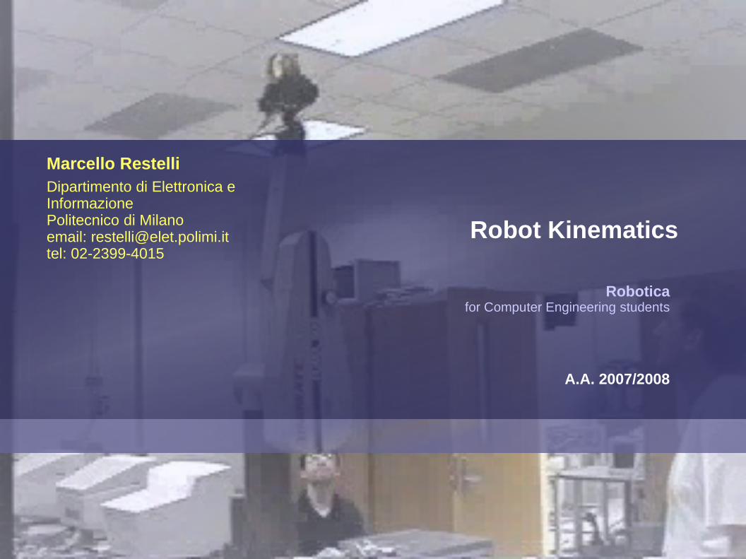
A.A. 2007/2008

Roboticafor Computer Engineering students

Marcello RestelliDipartimento di Elettronica e InformazionePolitecnico di Milanoemail: restelli@elet.polimi.ittel: 02-2399-4015

Robot Kinematics

2

Study of Motion

Kinematics studies the relation between the independent variables of the joints and the Cartesian positions reached by the robotDynamics studies the equations that characterize the robot motion (speed and acceleration)Trajectories computation consists of determining a way provide a robot for the sequence of points (or joint variables) to move from one point to another (kinematics) with suitable speeds and accelerations (dynamics)Control aims at performing trajectories that are similar to those computed

3

Kinematics

Two types of kinematics:Forward kinematics (angles to position):

what are you given:the length of each link

the angle of each joint

what you can find:the position of any point (i.e., its (x,y,z) coordinates)

Inverse Kinematics (position to angle):what are you given:

the length of each link

the position of some point on the robot

what you can findthe angles of each joint needed to obtain that position

4

Forward Kinematics: Example with Planar RR

Situationyou have a robotic arm that starts aligned with the x

0-axis

you tell the first link to move by θ1 and the second link to

move by θ2

The quest:what is the position of the end of the robotic arm?

Solution:Geometric approach

easier in simple situationsAlgebraic approach

involves coordinate transformations

5

Forward Kinematics: Example with 3 link arm

Situationyou have a 3 link arm that starts aligned with the x-axisl1,l

2,l

3 are the lengths of the 3 links

The three links are moved respectively by θ1, θ

2, θ

3

The questFind the Homogeneous matrix to get the position of the yellow dot in the X0Y0 frame

Solution H = Rz(θ1

) * Tx1(l1) * Rz(θ2) * Tx2(l2) * Rz(θ3

)

multiplying H by the position vector of the yellow dot in the X3Y3 frame gives its coordinates relative to the X0Y0 frame

X2\

X3Y2

Y3

θ1

θ2

θ3

1

2 3

X1

X0

Y0

6

Forward Kinematics

With more than 3 joints and with kinematic chains that do not lay on the plane the geometric method is too difficultWe need a systematic method:

represent the open kinematic chain with the same formalismfind algebraic solutions

using homogeneous coordinatesbuild references using a quasi-algorithmic procedure

Denavit-Hartenberg Notation

7

Denavit-Hartenberg Notation

Each joint is assigned a coordination frame

Using the Denavit-Hartenberg notation, you need 4 parameters to describe how a frame (i) relates to a previous frame ( i -1 )To align two axes we need 4 parameters: α, a, d, θ

8

The Parameters

1) ai

Technical definition: is the length of the perpendicular between the joint axes. The joint axes is the axes around which revolution takes place which are the Z(i-1) and Zi axes. These two axes can be viewed as lines in space. The common perpendicular is the shortest line between the two axis-lines and is perpendicular to both axis-lines.

9

The Parameters

1) ai

Visual approach: “A way to visualize the link parameter ai is to imagine an expanding cylinder whose axis is the Z(i-1) axis - when the cylinder just touches the joint axis i the radius of the cylinder is equal to ai ”(Manipulator Kinematics)

10

The Parameters

1) ai

It’s Usually on the Diagram Approach: If the diagram already specifies the various coordinate frames, then the common perpendicular is usually the X(i-1) axis. So ai is just the displacement along the X(i-1) to move from the i-1 frame to the i frame.If the link is prismatic, then ai is a variable

11

The Parameters

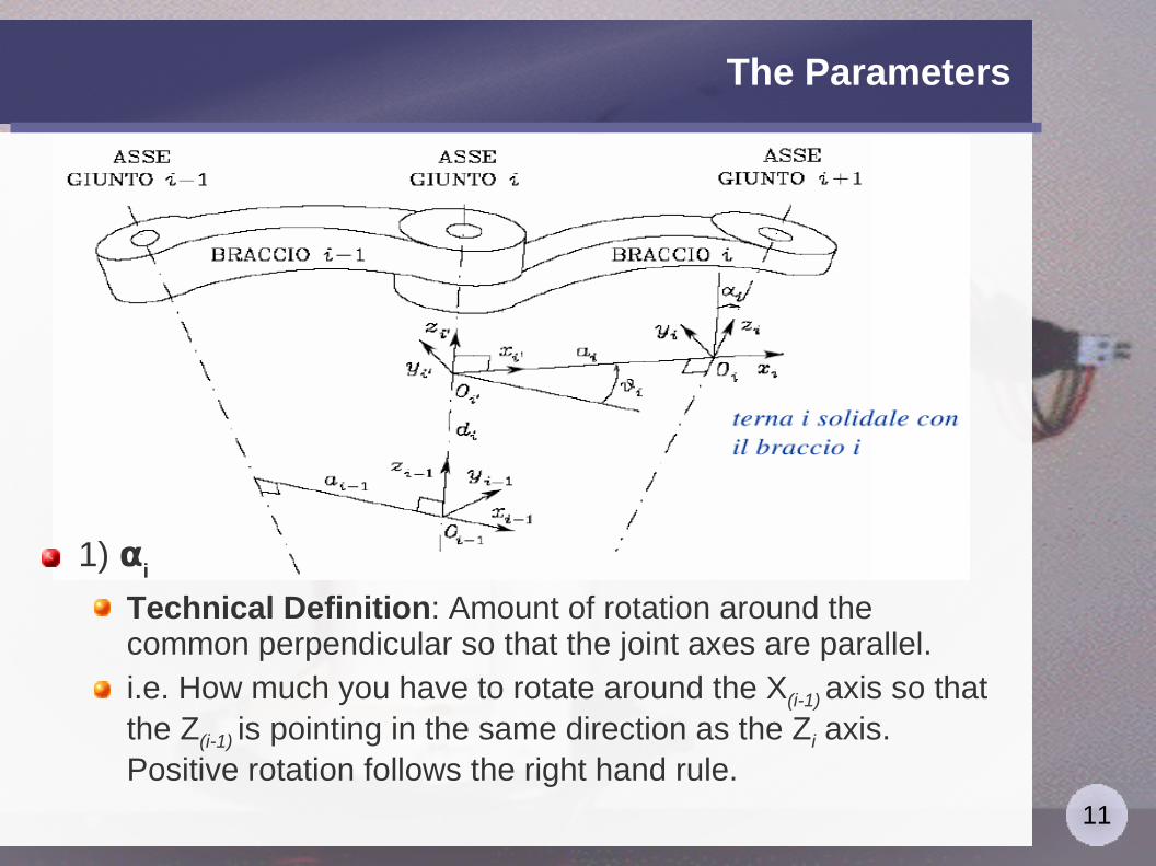
1) αi

Technical Definition: Amount of rotation around the common perpendicular so that the joint axes are parallel.i.e. How much you have to rotate around the X(i-1) axis so that the Z(i-1) is pointing in the same direction as the Zi axis. Positive rotation follows the right hand rule.

12

The Parameters

1) di

Technical Definition: The displacement along the Zi axis needed to align the a(i-1) common perpendicular to the ai

common perpendicular.In other words, displacement along the Zi to align the X(i-1) and Xi axes.

13

The Parameters

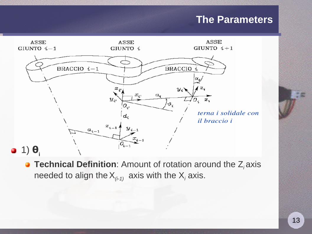
1) θi

Technical Definition: Amount of rotation around the Zi axis needed to align the X(i-1) axis with the Xi axis.

14

The Denavit-Hartenberg Matrix

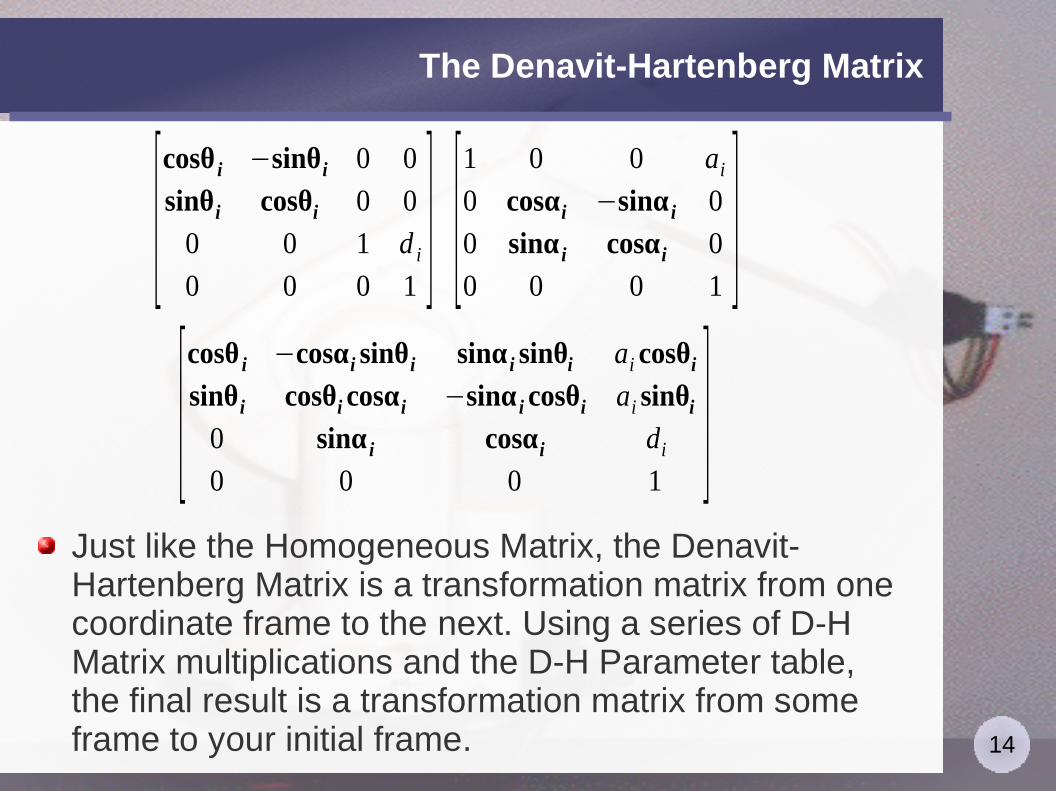
Just like the Homogeneous Matrix, the Denavit-Hartenberg Matrix is a transformation matrix from one coordinate frame to the next. Using a series of D-H Matrix multiplications and the D-H Parameter table, the final result is a transformation matrix from some frame to your initial frame.

[cosθ i −cosαi sinθi sinα i sinθi ai cosθisinθi cosθi cosαi −sinα i cosθi ai sinθi0 sinα i cosαi di

0 0 0 1]

[cosθ i −sinθi 0 0

sinθi cosθi 0 0

0 0 1 d i

0 0 0 1] [1 0 0 ai

0 cosαi −sinα i 0

0 sinα i cosαi 0

0 0 0 1]

15

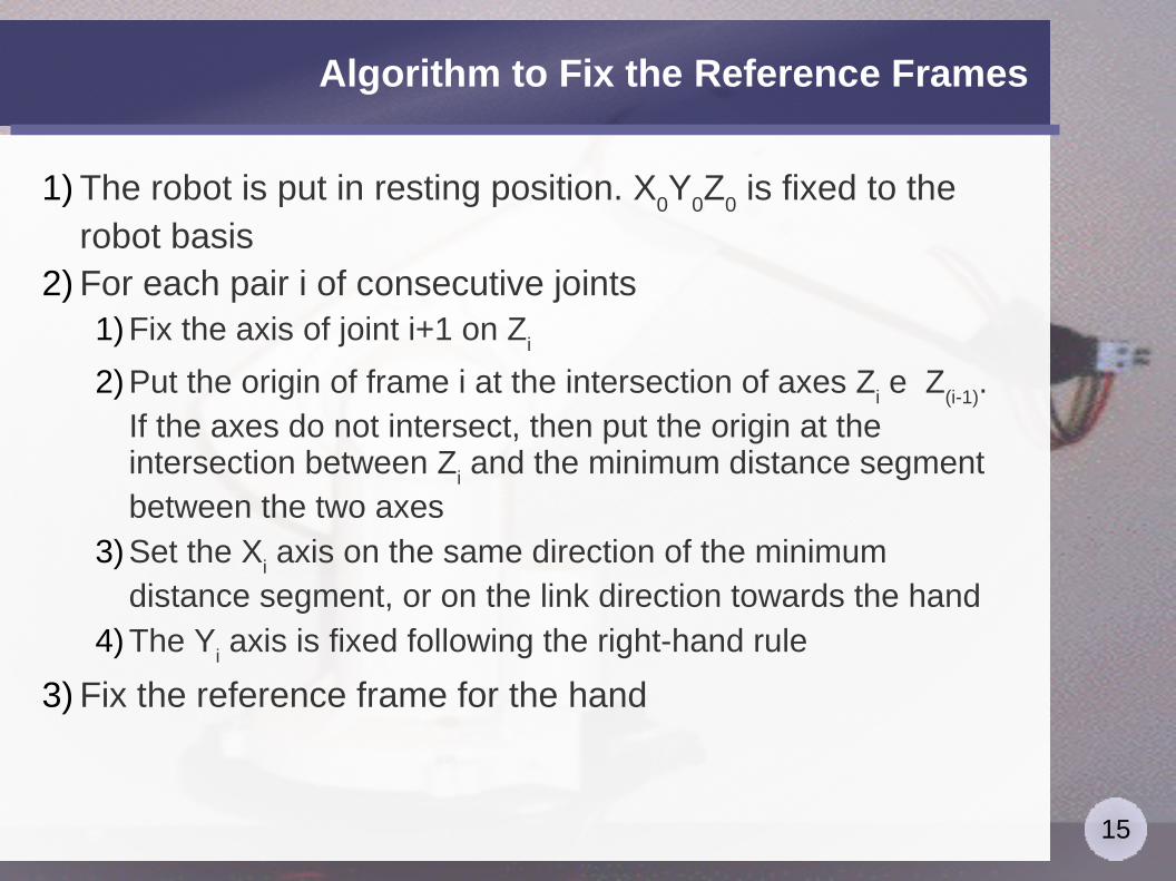
Algorithm to Fix the Reference Frames

1) The robot is put in resting position. X0Y

0Z

0 is fixed to the

robot basis2) For each pair i of consecutive joints

1) Fix the axis of joint i+1 on Zi

2) Put the origin of frame i at the intersection of axes Zi e Z

(i-1).

If the axes do not intersect, then put the origin at the intersection between Z

i and the minimum distance segment

between the two axes3) Set the X

i axis on the same direction of the minimum

distance segment, or on the link direction towards the hand4) The Y

i axis is fixed following the right-hand rule

3) Fix the reference frame for the hand

16

Algorithm to Fix the Reference Frames

4) For each pair i of consecutive reference frames compute the four parameters1) Compute d

i: distance between axes X

(i-1) and X

i along axis

Z(i-1)

(variable for a prismatic joint)

2) Compute a(i-1)

: distance between axes Z(i-1)

and Zi along axis

Xi (link length)

3) Compute θi: revolution angle between X

(i-1) and X

i around

axis Z(i-1)

(variable for a revolute joint)

4) Compute α(i-1)

: revolution angle between Z(i-1)

and Zi around

axis Xi (twist angle)

17

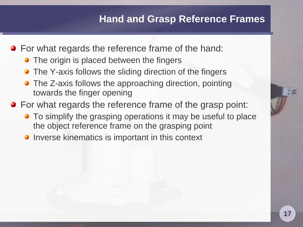
Hand and Grasp Reference Frames

For what regards the reference frame of the hand:The origin is placed between the fingersThe Y-axis follows the sliding direction of the fingersThe Z-axis follows the approaching direction, pointing towards the finger opening

For what regards the reference frame of the grasp point:To simplify the grasping operations it may be useful to place the object reference frame on the grasping pointInverse kinematics is important in this context

18

Algorithm for Forward Kinematics

1) Put the manipulator in resting position2) Set the reference frames to joints and links3) Compute Denavit-Hartenberg parameters4) Compute transformation matrix A

i that allows to pass from

the reference frame of the i-th joint to the one of the (i+1)-th joint

5) Multiply matrices Ai to get matrix T that allows to pass from

the reference frame of the base X0Y

0Z

0 to the one of the

hand XnY

nZ

n

6) From the matrix T extract the coordinates of the current position

7) Look at the rotation sub-matrix and extract orientation components

19

Transformation Matrix A

The transformations required to pass from reference frame i-1 to reference frame i w.r.t. joint i-1 are:

Rotate X(i-1)

by θi around Z

(i-1), to align it with X

i: Rot(Z

(i-1),θ

i)

Translate the origin of reference frame i-1 by di along Z

(i-1),

to overlap X(i-1)

and Xi: Transl(0,0,d

i)

Translate the origin of reference frame i-1 by ai along X

i, to

place it at the origin of reference frame i: Transl(ai,0,0)

Rotate Z(i-1)

around Xi by α

i to overlap the two reference

frames i-1 and i: Rot(Xi,α

i)

Ai-1,i

i-1 = Transl(0,0,di)*Rot(Z

(i-1),θ

i)*Transl(a

i,0,0)*Rot(X

i,α

i)

20

Transformation Matrix A

Revolute joint

Prismatic joint

[cosθ i −cosαi sinθi sinα i sinθi ai cosθisinθi cosθi cosαi −sinα i cosθi ai sinθi0 sinα i cosαi di

0 0 0 1]

[cosθ i −cosαi sinθi sinα i sinθi 0

sinθi cosθi cosαi −sinα i cosθi 0

0 sinα i cosαi d i

0 0 0 1]

21

Transformation Matrix T

Aim: given a point in the mobile system, we want its coordinates in the fixed systemT = A

0,60 = A

0,10· A1,2

1· A2,32· A3,4

3· A4,54· A5,6

5

Pi-1 = Ai-1,ii-1· Pi

T=[x i yi zi pi0 0 0 1 ]=[R i pi

0 1 ]

22

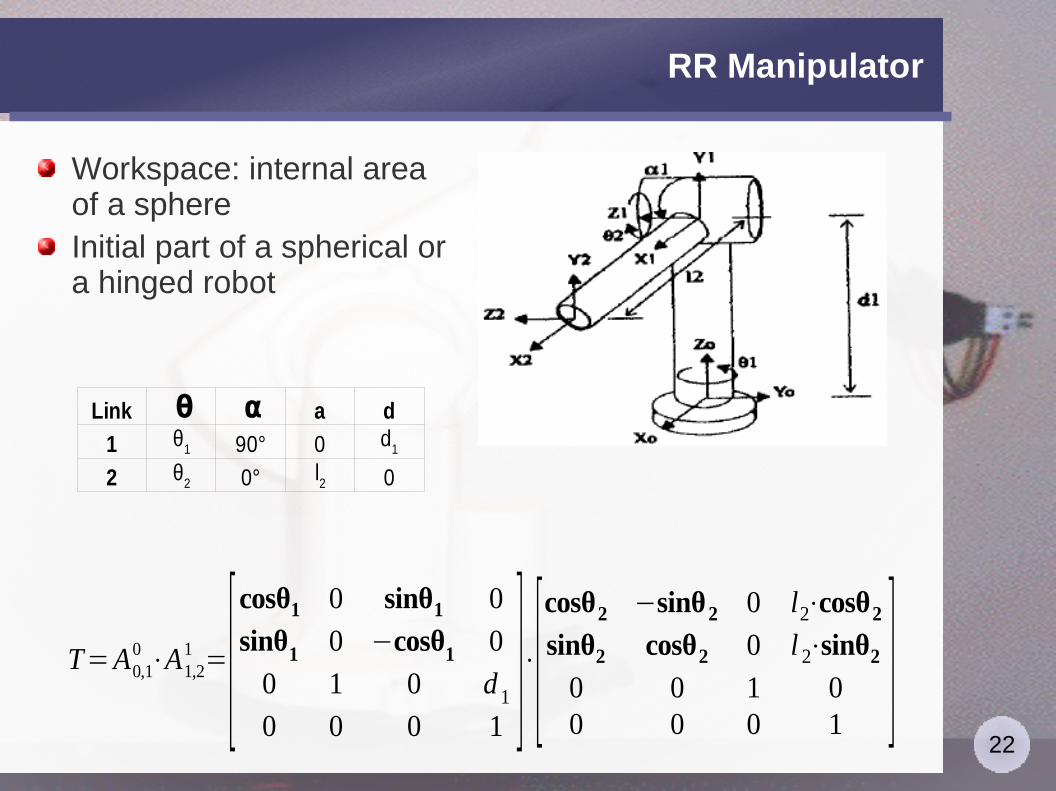
RR Manipulator

Workspace: internal area of a sphereInitial part of a spherical or a hinged robot

T=A0,10 ⋅A1,2

1 =[cosθ1 0 sinθ1 0

sinθ1 0 −cosθ1 0

0 1 0 d 10 0 0 1

]⋅[cosθ2 −sinθ2 0 l2⋅cosθ2sinθ2 cosθ2 0 l 2⋅sinθ20 0 1 00 0 0 1

]

Link θ α a d

1 90° 0

2 0° 0

θ1

d1

θ2

l2

23

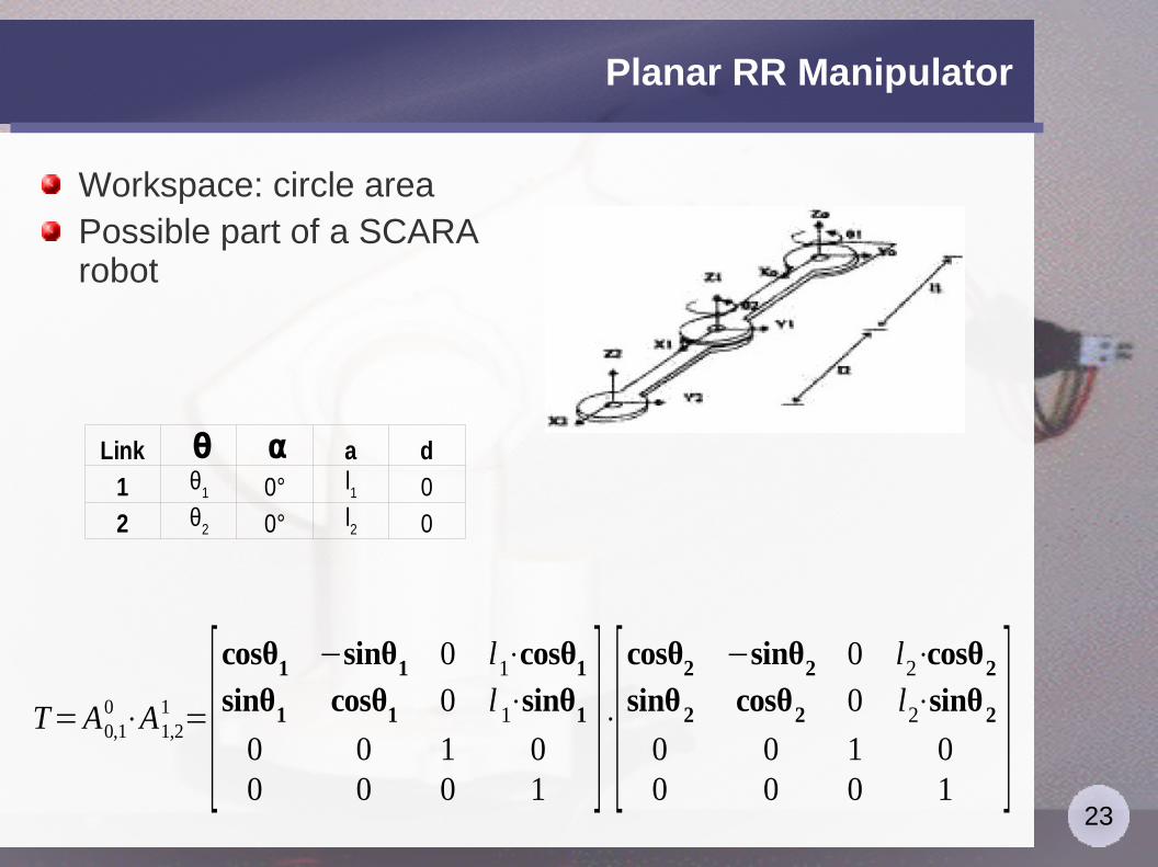
Planar RR Manipulator

Workspace: circle areaPossible part of a SCARA robot

T=A0,10 ⋅A1,2

1 =[cosθ1 −sinθ1 0 l1⋅cosθ1sinθ1 cosθ1 0 l 1⋅sinθ10 0 1 00 0 0 1

]⋅[cosθ2 −sinθ2 0 l2⋅cosθ2sinθ2 cosθ2 0 l2⋅sinθ20 0 1 00 0 0 1

]

Link θ α a d

1 0° 0

2 0° 0

θ1

l1

θ2

l2

24

RT Manipulator

Workspace: circle areaPossible part of a cylindric robot

T=A0,10 ⋅A1,2

1 =[cosθ1 0 sinθ1 0

sinθ1 0 −cosθ1 0

0 1 0 d 10 0 0 1

]⋅[1 0 0 00 1 0 00 0 1 d 20 0 0 1

]

Link θ α a d

1 90° 0

2 0° 0° 0

θ1

d1

d2

25

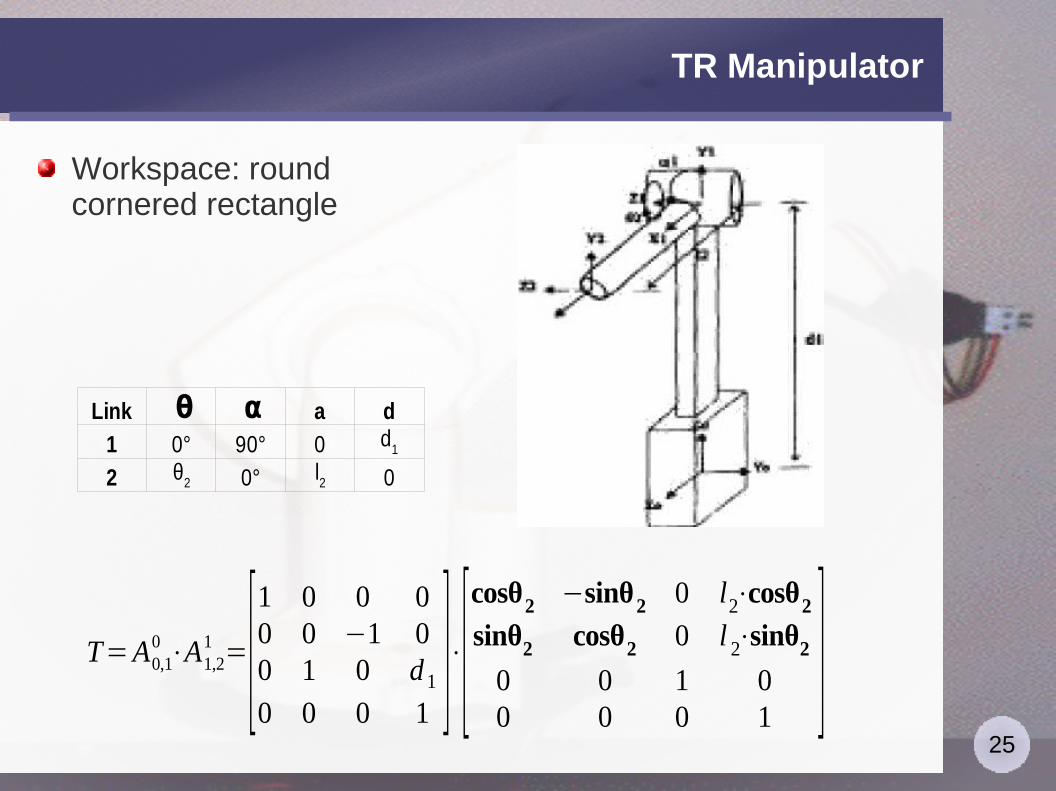
TR Manipulator

Workspace: round cornered rectangle

T=A0,10 ⋅A1,2

1 =[1 0 0 00 0 −1 00 1 0 d 10 0 0 1

]⋅[cosθ2 −sinθ2 0 l2⋅cosθ2sinθ2 cosθ2 0 l 2⋅sinθ20 0 1 00 0 0 1

]

Link θ α a d

1 0° 90° 0

2 0° 0

d1

θ2

l2

26

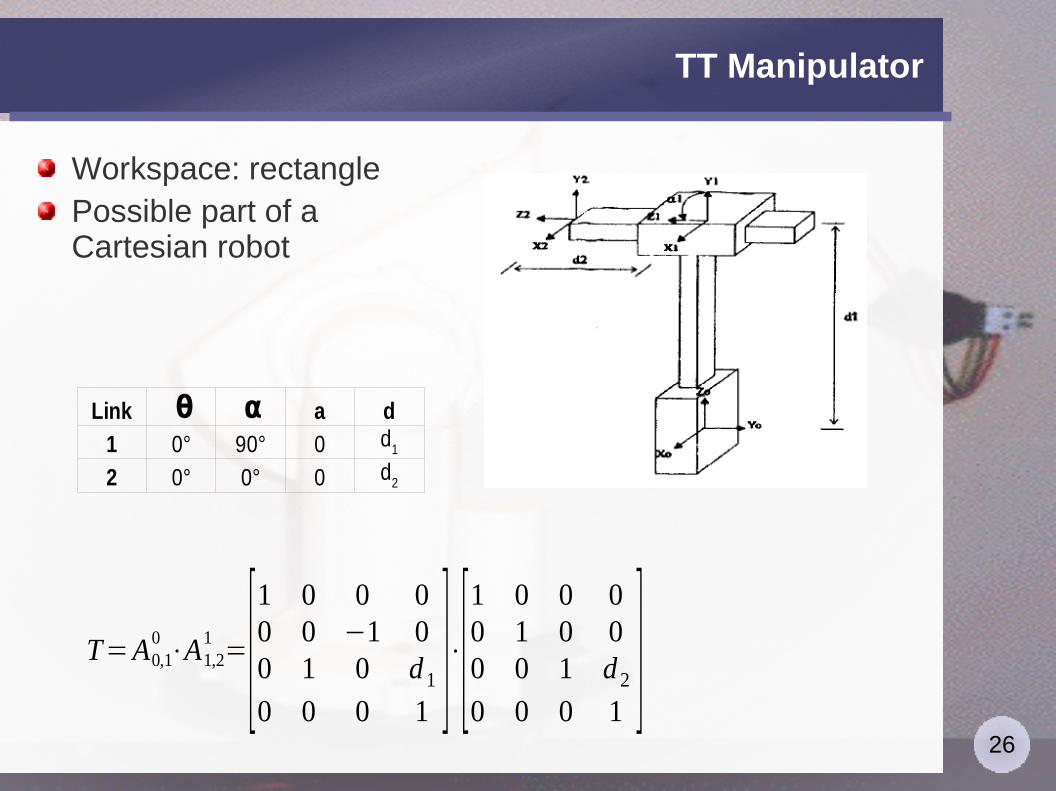
TT Manipulator

Workspace: rectanglePossible part of a Cartesian robot

T=A0,10⋅A1,2

1=[1 0 0 00 0 −1 00 1 0 d 10 0 0 1

]⋅[1 0 0 00 1 0 00 0 1 d 20 0 0 1

]

Link θ α a d

1 0° 90° 0

2 0° 0° 0

d1

d2

27

Hand Orientation

We use the Euler's angles...

... and equal them to the orientation sub-matrix:

R=Rot z ,⋅Rot u ,⋅Rot w ,=

=[coscos−sincos sin −cos sin−sin cos cos sin sin

sincoscoscos sin −sin sincos cos cos −cossin

sin sin sin cos cos ]

T=[x i yi zi pi0 0 0 1 ]=[R i pi

0 1 ]

R i=[nx ox axn y o y a ynz oz a z

]

28

Hand Orientation: A Simple Solution

A simple solution can be obtained by solving the set of 9 equations and 3 unknown quantities

This solution is useless:the accuracy of arccos function depends by the angle since cos(θ) = cos(-θ)

when θ approaches 0° or 180° the last two equations give inaccurate or indefinite solutions

=cos−1[az ]

=cos−1 [ o z

sin ]=cos−1 [−a y

sin ]

29

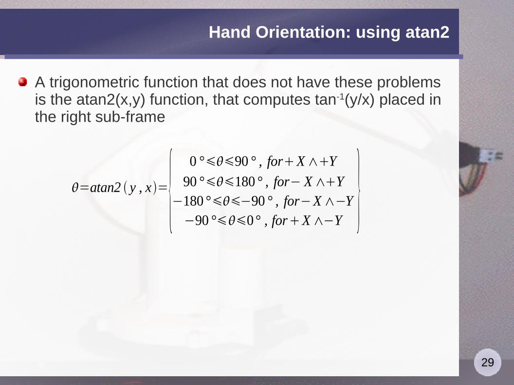
Hand Orientation: using atan2

A trigonometric function that does not have these problems is the atan2(x,y) function, that computes tan-1(y/x) placed in the right sub-frame

=atan2 y , x={0 °90 ° , forX∧Y

90 °180 ° , for− X∧Y−180 °−90 ° , for−X∧−Y−90 °0° , forX∧−Y

}

30

Hand Orientation: Paul Method

The Paul method computes the hand orientation using the atan2 functionThe method consists of pre-multiplying both ends of equation by the inverse of one of the rotation matrices.

Now Φ is on the left side

R z ,−1

⋅[n x ox axn y o y a ynz o z az

]=Ru ,⋅R w ,

= tan−1 [ ax

−a y ]=atan2 ax ,−a y

= tan−1 [ sincos ]= tan−1 [−ox cos−o y sin

nx cosny sin ]=atan2 −ox cos−o y sin ,nx cosn y sin

= tan−1[ sin cos ]=tan−1 [ax sin−ay cos

az ]=atan2 ax sin−a y cos ,az

31

Hand Orientation: Paul Method

The same method can be applied trough post-multiplying both ends of equation by the inverse of one of the rotation matrices.

We do not know when it it is better to use the pre or the post-method

[nx o x axn y o y a ynz oz a z

]⋅Rw ,−1=R z ,⋅Ru ,

= tan−1 [ nz

oz ]=atan2 nz ,oz

=tan−1 [ sincos ]= tan−1 [ ny coso y sin

nx cosox sin ]=atan2 n ycosoy sin , nx cosox sin

= tan−1[ sin cos ]=tan−1 [nz sinoz cos

az ]=atan2 nz sinoz cos ,az

32

Forward Kinematics: Conclusions

The forward kinematic problem has always one and only one solution, that can be obtain through the computation of transformation matrix TSince T is obtained through the product of 6 matrices, for computational reasons use only two matrices:

one for the 3 DOF of the armone for the 3 DOF of the hand

Nevertheless there are still some real-time problems to compute the Cartesian coordinates

Often joint variables are used

33

Inverse Kinematics: Problem Formulation

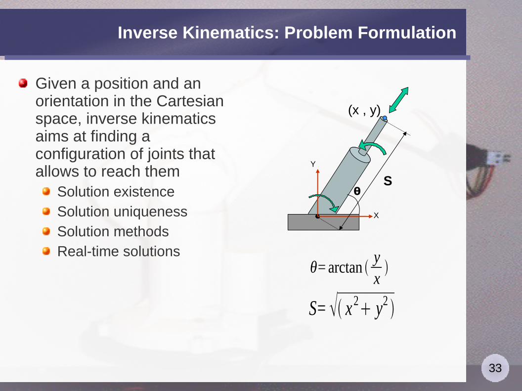
Given a position and an orientation in the Cartesian space, inverse kinematics aims at finding a configuration of joints that allows to reach them

Solution existenceSolution uniquenessSolution methodsReal-time solutions

θ

X

Y

S

(x , y)

θ=arctan yx

S= x2 y2

34

Inverse Kinematics: the Solution

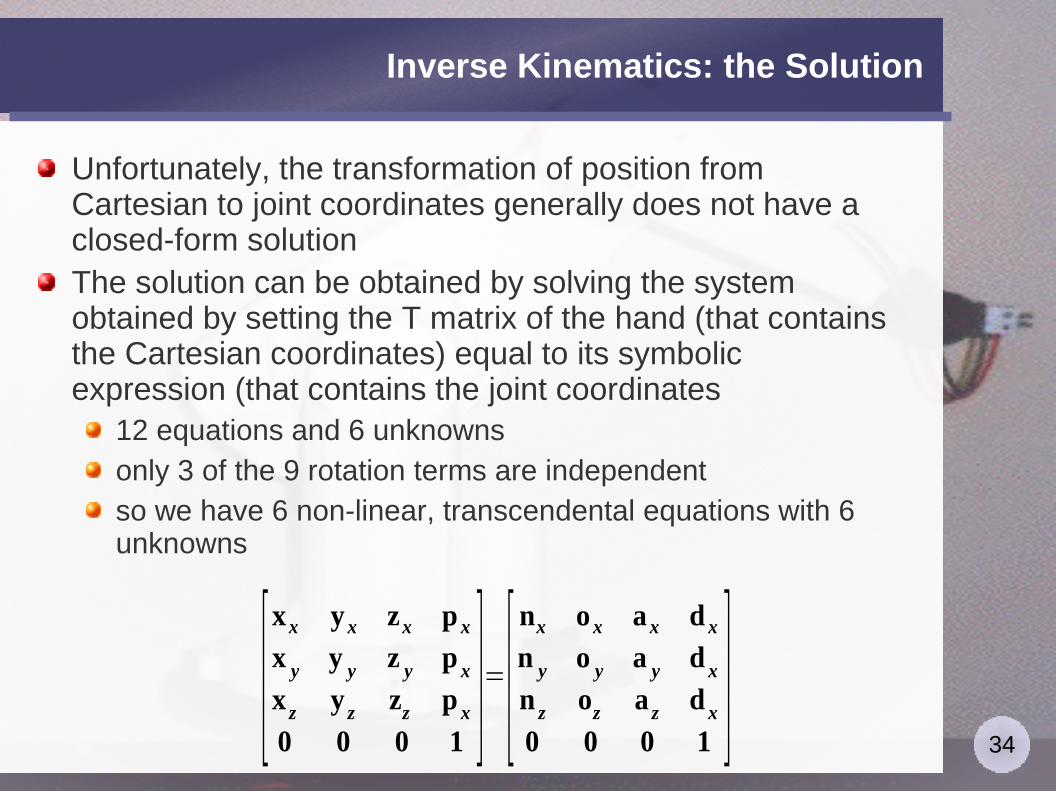
Unfortunately, the transformation of position from Cartesian to joint coordinates generally does not have a closed-form solutionThe solution can be obtained by solving the system obtained by setting the T matrix of the hand (that contains the Cartesian coordinates) equal to its symbolic expression (that contains the joint coordinates

12 equations and 6 unknownsonly 3 of the 9 rotation terms are independentso we have 6 non-linear, transcendental equations with 6 unknowns

[xx y x zx p xx y y y z y p xx z y z zz p x0 0 0 1

]=[nx o x a x d xn y o y a y d xn z oz a z d x0 0 0 1

]

35

Inverse Kinematics: Solution Existence

If the point to be reached falls into the workspace and the robot has 6 DOF then a solution existsIf the robot has less than 6 DOF it has to be verified that the point can be reachedIt is hard to determine whether a point falls or not inside the workspaceThings are even harder when considering the dexterous spaceThe solution does not exist when:

the goal point is outside the workspacethe goal point is inside the workspace but there are physical constraintsthe goal point must be reached following a trajectory that requires infinite acceleration

36

Inverse Kinematics: Solution Uniqueness

What makes Inverse Kinematics a hard problem?Redundancy: a uniques solution to this problem does not existThe number of possible solutionsincreases with the number of DOFThe number of solutionsdepends by the number of Denavit-Hartenberg non-null parameters

For a 6R manipulator we may have at most 16 solutions

We are interested in all the possible solutionswe need a criterion to select the best solution:

the “closest” to the current configurationmove outermost links the mostenergy minimizationminimum time

(x , y)l2

l1l2

l1

37

Inverse Kinematics: Solution Methods

Several solution methods have been proposed:Closed form solutions

Geometrical methodsreduce the larger problem to a series of plane geometry problems

Algebraic methodstrigonometric equations

Iterative (numerical) solutions

38

Geometrical Method: An Example

Using the law of cosines:

Using the law of sines:

l1

l2θ2

θ1

α

(x , y)

x 2 y2 =l12l2

2−2 l1 l 2cos −2

2=arccos x2 y 2−l1

2−l2

2

2 l1 l2 : REDUNDANT

sin 1−

l2=sin −2

x2 y2=sin 2

x 2 y2

1=arcsin l2sin 2 x2 y2 atan2 y , x: REDUNDANCY caused by the two values of 2

39

Algebraic Method: The Same Example

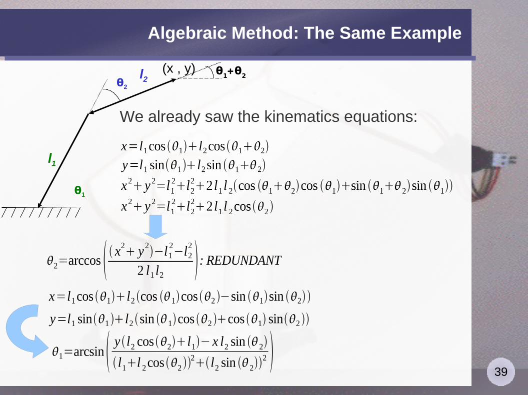
We already saw the kinematics equations:

l1

l2θ2

θ1

θ1+θ2(x , y)

x=l1cos 1l2cos12

y=l1 sin1 l2sin 12

x 2 y 2=l12l2

22 l1 l 2cos 12cos 1sin 12sin 1

x 2 y 2=l12l2

22 l1 l 2cos2

2=arccos x2 y 2−l1

2−l2

2

2 l1 l2 : REDUNDANT

x=l1cos 1l2 cos 1cos2 −sin 1sin 2

y=l1 sin1 l2 sin 1cos 2 cos 1 sin2

1=arcsin y l2 cos2l1− x l2 sin 2

l1l 2cos 2 2 l2 sin 2

2

40

Inverse Kinematics: Closed Form Solutions

An arbitrary 6 DOF manipulator cannot be solved using a closed form solutionPieper's method: solution of a 4th order polynomialPaul's method: pre- and post-multipliesOther methods

helicoidal algebradouble matricesquaternionsalgebraic approaches based on substitutions

u = tan(θ/2)cos(θ) = (1-u2)/(1+u2)sin(θ) = 2u/(1+u2)

41

Inverse Kinematics: Pieper's Solution

Suitable for manipulators with 6 DOF in which 3 consecutive axes intersect at a point (including robots with 3 consecutive parallel axes, since they met at a point at infinity)Pieper's method applies to the majority of commercially available industrial robots (Puma 560, SCARA)The Pieper's solution computes separately the first 3 and the last 3 joints:

Locate the intersection of the last 3 joint axesSolve IK for first 3 jointsCompute T

0,3 and determine T

3,6 as T

0.3'T

0.6

Solve IK for last three joints

42

Inverse Kinematics: Paul's Solution

Set the known Cartesian matrix T equal to the manipulator matrix (containing the joint unknowns)Search the second matrix for:

Elements with only one joint unknownPair of elements that lead to an expression with only one unknown once divided by each otherElements that can be simplified

Solve the equations involving the selected elements, thus finding joint unknowns as function of known elements belonging to the T matrixIf no element has been identified at step 2, pre-multiply both terms for the inverse of the transformation matrix of the first link (and iteratively for the following links)

as an alternative it is possible to post-multiply for the inverse of the transformation matrix of the last link

43

Example of Paul's method: RR

Select px e p

y

Pre-multiply by (A0,1

0)-1

T=[cosθ1 cosθ2 −cosθ1 sinθ2 sinθ1 l2 cosθ1 cosθ2sinθ1 cosθ2 −sinθ1 sinθ2 −cosθ1 l2 sinθ1 cosθ2sinθ2 cosθ2 0 d 1l 2 sinθ20 0 0 1

]=[n x ox a x pxn y o y a y p yn z o z a z p z0 0 0 1

]p y

p x

=l2⋅sen θ1 ⋅cos θ2

l2⋅cos θ1⋅cosθ2 ⇒θ1=tan

−1 p y

px

p x⋅cos θ1 p y⋅sin θ1

pz−d 1=

l2⋅cos θ 2

l2⋅sin θ 2 ⇒θ 2=tan

−1 p z−d 1p x⋅cos θ1 p y⋅sin θ1

44

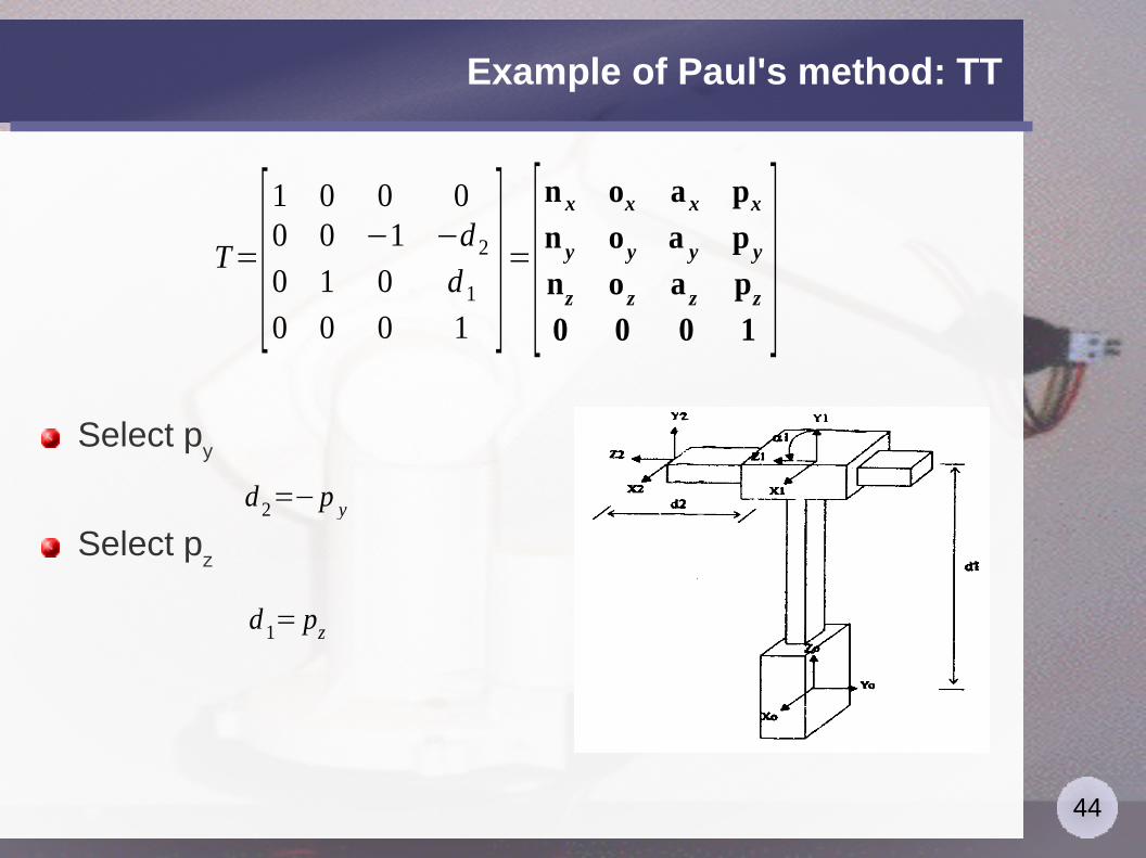
Example of Paul's method: TT

Select py

Select pz

T=[1 0 0 00 0 −1 −d 20 1 0 d 10 0 0 1

]=[n x ox a x pxn y o y a y p ynz o z a z pz0 0 0 1

]d 2=−p y

d 1= pz

45

Iterative Solutions

For robots with coupled geometries the closed form solution may not exist => iterative solutions

m equations with n unknownsit starts with an initial estimationcompute T matrix and error w.r.t. Cartesian valuesupdate the estimate to reduce the errorindefinite execution time to get a definite error or indefinite error to get a definite execution timeiterative methods may fail to find all the solutions to IK

While in the '80s these methods were not feasible, nowadays they represent an alternativeNevertheless, industrial robots are typically built to meet one of the Pieper's sufficient conditions in order to use closed form solutions

46

Redundancies and Degenerations

A manipulator is redundant if it can reach the same position with several different configurationsManipulators with more of 6 DOF are infinitely redundantA point reachable with infinite configurations is called degeneration pointPhysical constraints are imposed to avoid degeneration points

47

Static Precision

Accuracydifference between desired position and actually reached positionless tolerance => higher accuracy

Repeatabilitythe variance of the reached position while repeating the same commandimportant when the robot is programmed on the field

Spatial resolutionthe minimum distance that can be measured or commandedit depends by the resolution of the internal sensors

48

Manipulator Performances

Maximum payloadthe maximum weight that can be carried by a robot at low speed while keeping the accuracythe nominal payload is measured at maximum speed while keeping the accuracythe payload is any weight put on the wrist

Maximum speedthe maximum velocity at which the robot end can be moved while extended

Cycle timeThe cycle time is the time required to execute a standard cycle of pick-and-place of 12 inchesFor industrial robots ~ 1s