Semantic Foundations for Heterogeneous Systems

by

Roberto Passerone

Laurea (Politecnico di Torino) 1994M. S. (University of California, Berkeley) 1997

A dissertation submitted in partial satisfaction of the

requirements for the degree of

Doctor of Philosophy

in

Engineering - Electrical Engineering and Computer Sciences

in the

GRADUATE DIVISION

of the

UNIVERSITY OF CALIFORNIA, BERKELEY

Committee in charge:Professor Alberto L. Sangiovanni-Vincentelli, Chair

Professor Jan M. RabaeyProfessor Theodore A. Slaman

Doctor Jerry R. Burch

Spring 2004

The dissertation of Roberto Passerone is approved:

Chair Date

Date

Date

Date

University of California, Berkeley

Spring 2004

Semantic Foundations for Heterogeneous Systems

Copyright 2004

by

Roberto Passerone

1

Abstract

Semantic Foundations for Heterogeneous Systems

by

Roberto Passerone

Doctor of Philosophy in Engineering - Electrical Engineering and Computer Sciences

University of California, Berkeley

Professor Alberto L. Sangiovanni-Vincentelli, Chair

The ability to incorporate increasingly sophisticated functionality makes the design of electronic

embedded systems complex. Many factors, beside the traditional considerations of cost and perfor-

mance, contribute to making the design and the implementation of embedded systems a challenging

task. The inevitable interactions of an embedded system with the physical world require that its parts

be described by multiple formalisms of heterogeneous nature. Because these formalisms evolved in

isolation, system integration becomes particularly problematic. In addition, the computation, often

distributed across the infrastructure, is frequently controlled by intricate communication mecha-

nisms. This, and other safety concerns, demand a higher degree of confidence in the correctness of

the design that imposes a limit on design productivity.

The key to addressing the complexity problem and to achieve substantial productivity

gains is a rigorous design methodology that is based on the effective use of decomposition and mul-

tiple levels of abstraction. Decomposition relies on models that describe the effect of hierarchically

composing different concurrent parts of the system. An abstraction is the relationship between two

representations of the same system that expose different levels of detail. To maximize their benefit,

these techniques require a semantic foundation that provides the ability to formally describe and re-

late a wide range of concurrency models. This Dissertation proposes one such semantic foundation

in the form of an algebraic framework called Agent Algebra.

Agent Algebra is a formal framework that can be used to uniformly present and reason

about the characteristics and the properties of the different models of computation used in a design,

and about their relationships. This is accomplished by defining an algebra that consists of a set of

denotations, called agents, for the elements of a model, and of the main operations that the model

2

provides to compose and to manipulate agents. Different models of computation are constructed as

distinct instances of the algebra. However, the framework takes advantage of the common algebraic

structure to derive results that apply to all models in the framework, and to relate different models

using structure-preserving maps.

Relationships between different models of computation are described in this Dissertation

as conservative approximations and their inverses. A conservative approximation consists of two ab-

stractions that provide different views of an agent in the form of an over- and a under-approximation.

When used in combination, the two mappings are capable of preserving refinement verification re-

sults from a more abstract to a more concrete model, with the guarantee of no false positives.

Conservative approximations and their inverses are also used as a generic tool to construct a cor-

respondence between two models. Because this correspondence makes the correlation between an

abstraction and the corresponding refinement precise, conservative approximations are useful tools

to study the interaction of agents that belong to heterogeneous models. A detailed comparison also

reveals the necessary and sufficient conditions that must be satisfied for the well established notions

of abstract interpretations and Galois connections (in fact, for a pair thereof) to form a conservative

approximation. Conservative approximations are illustrated by several examples of formalization

of models of computation of interest in the design of embedded systems.

While the framework of Agent Algebra is general enough to encompass a variety of

models of computation, the common structure is sufficient to prove interesting results that ap-

ply to all models. In particular, this Dissertation focuses on the problem of characterizing the

specification of a component of a system given the global specification for the system and the

context surrounding the component. This technique, called Local Specification Synthesis, can be

applied to a solve synthesis and optimization problems in a number of different application ar-

eas. The results include sufficient conditions to be met by the definitions of system composition

and system refinement for constructing such characterizations. The local specification synthe-

sis technique is also demonstrated through its application to the problem of protocol conversion.

Professor Alberto L. Sangiovanni-VincentelliDissertation Committee Chair

i

To the ones I love

ii

Acknowledgments

I get to put my name on the cover of this dissertation, but many are the people who contributed in

part to the work and who supported me during these years. Without them, it wouldn’t have been

nearly as much fun.

First, I would like to thank Prof. Alberto Sangiovanni-Vincentelli for the privilege of

having him as my research advisor during my career as a student at UC Berkeley. He is the one

“responsible” for getting me started on this project and for getting me excited about it during all

these years. While giving me a lot of freedom in shaping the research direction, he was relentless in

keeping it on track. Alberto taught me what research is all about.

A special thank goes to Dr. Jerry Burch. His influence and contributions were critical

in many situations and are spread throughout this work. Jerry showed me how to do research and

how to look at problems from different perspectives. Our long discussions over the phone, at times

intense, and always stimulating, have had a profound impact on the way I approach a problem, both

in and outside research. His style is for me the model to be followed in any future endeavor.

I would like to thank Prof. Jan Rabaey and Prof. Ted Slaman for serving as members

of my Dissertation Committee. I am grateful to Jan for getting me involved with his group at the

BWRC, and for being a constant reminder that, in the end, we need “things that work”. I am grateful

to Ted for introducing me to the mysteries of logic and recursive functions, and for our delightful

discussions over lunch.

I would like to thank all the staff at UC Berkeley, and in particular Flora Oviedo, Jennifer

Stone, Lorie Brofferio, Mary Byrnes and Ruth Gjerde. If the students can get anything accomplished

it is because of their support.

During my career as a graduate student I had the opportunity to meet some of the finest

people there are. I would like to thank all the past and present members of Cadence’s VCC group

and of the Cadence Laboratories in Berkeley with whom I have shared these years of professional

life; I am indebted to all the students and the staff of the Berkeley Wireless Research Center for the

many pleasant hours spent at the center and for the exciting retreats; I want to thank the members and

the staff of the GSRC for promoting such interesting research and for organizing thought-provoking

meetings and workshops; and last but not least I am especially grateful to all the occupants of the

old 550 Cory Hall and to my office mates in 545 Cory Hall. In particular I would like to extend

a special thank to Alessandra Nardi, Alessandro Pinto, Alex Kondratyev, Claudio Pinello, Doug

Densmore, Elaine Cheong, Farinaz Koushanfar, Felice Balarin, Fernando De Bernardinis, Gerald

iii

Wang, Grant Martin, Guang Yang, Harry Hsieh, Huifang Qin, Jorn Janneck, Jerry Burch, Julio Silva,

Luca Carloni, Luca Daniel, Luciano Lavagno, Luigi Palopoli, Marco Sgroi, Marlene Wan, Massimo

Baleani, Max Chiodo, Mike Sheets, Mukul Prasad, Naji Ghazal, Paolo Giusto, Peggy Laramie,

Perry Alexander, Rong Chen, Rupak Majumdar, Subarna Sinha, Suet-Fei Li, Trevor Meyerowitz,

Vandana Prabhu, Yanmei Li and Yoshi Watanabe. It is the calibre of these people and the warmth

of their friendship that makes this a great place to live.

But foremost I owe the very chance of coming to Berkeley in the first place to the support

of my wife Barbara. I was fortunate to have her by my side during these years. The accomplishments

of this work are hers as much as mine. And life has taken a whole new meaning with the arrival of

our son Davide. It is with his smile in our hearts that we bring this work to a close. Barbara and

Davide are indispensable ingredients of my life.

iv

Contents

List of Figures vii

List of Definitions ix

1 Introduction 11.1 Models of Computation and Semantic Domains . . . . . . . . . . . . . . . . . . . 31.2 Levels of Abstraction . . . . . . . . . . . . . . . . . . . . . . . . . . . . . . . . . 51.3 Refinement Verification and Local Specification Synthesis . . . . . . . . . . . . . 7

1.3.1 Compatibility and Protocol Conversion . . . . . . . . . . . . . . . . . . . 101.4 Scope and Principles . . . . . . . . . . . . . . . . . . . . . . . . . . . . . . . . . 121.5 Major Results . . . . . . . . . . . . . . . . . . . . . . . . . . . . . . . . . . . . . 151.6 Motivating Example . . . . . . . . . . . . . . . . . . . . . . . . . . . . . . . . . 161.7 An Example Agent Algebra . . . . . . . . . . . . . . . . . . . . . . . . . . . . . . 18

1.7.1 Operations on Behaviors and Agents . . . . . . . . . . . . . . . . . . . . . 221.8 Related Work . . . . . . . . . . . . . . . . . . . . . . . . . . . . . . . . . . . . . 26

1.8.1 Algebraic Approaches . . . . . . . . . . . . . . . . . . . . . . . . . . . . 261.8.2 Trace Theory . . . . . . . . . . . . . . . . . . . . . . . . . . . . . . . . . 291.8.3 Tagged Signal Model . . . . . . . . . . . . . . . . . . . . . . . . . . . . . 301.8.4 Ptolemy II . . . . . . . . . . . . . . . . . . . . . . . . . . . . . . . . . . 311.8.5 Abstract Interpretations . . . . . . . . . . . . . . . . . . . . . . . . . . . . 331.8.6 Interface Theories . . . . . . . . . . . . . . . . . . . . . . . . . . . . . . 361.8.7 Process Spaces . . . . . . . . . . . . . . . . . . . . . . . . . . . . . . . . 391.8.8 Category Theoretic Approaches . . . . . . . . . . . . . . . . . . . . . . . 411.8.9 Rosetta . . . . . . . . . . . . . . . . . . . . . . . . . . . . . . . . . . . . 441.8.10 Hybrid Systems . . . . . . . . . . . . . . . . . . . . . . . . . . . . . . . . 441.8.11 Local Specification Synthesis . . . . . . . . . . . . . . . . . . . . . . . . 47

1.9 Outline of the Dissertation . . . . . . . . . . . . . . . . . . . . . . . . . . . . . . 49

2 Agent Algebras 532.1 Preliminaries . . . . . . . . . . . . . . . . . . . . . . . . . . . . . . . . . . . . . 542.2 Agent Algebras . . . . . . . . . . . . . . . . . . . . . . . . . . . . . . . . . . . . 562.3 Construction of Algebras . . . . . . . . . . . . . . . . . . . . . . . . . . . . . . . 612.4 Ordered Agent Algebras . . . . . . . . . . . . . . . . . . . . . . . . . . . . . . . 65

v

2.4.1 Construction of Algebras . . . . . . . . . . . . . . . . . . . . . . . . . . . 732.5 Agent Expressions . . . . . . . . . . . . . . . . . . . . . . . . . . . . . . . . . . 742.6 Relationships between Agent Algebras . . . . . . . . . . . . . . . . . . . . . . . . 78

2.6.1 Conservative Approximations . . . . . . . . . . . . . . . . . . . . . . . . 802.6.2 Inverses of Conservative Approximations . . . . . . . . . . . . . . . . . . 822.6.3 Compositional Conservative Approximations . . . . . . . . . . . . . . . . 85

2.7 Conservative Approximations Induced by Galois Connections . . . . . . . . . . . 972.7.1 Preliminaries . . . . . . . . . . . . . . . . . . . . . . . . . . . . . . . . . 972.7.2 Conservative Approximations and Galois Connections . . . . . . . . . . . 1062.7.3 Abstract Interpretations . . . . . . . . . . . . . . . . . . . . . . . . . . . . 111

2.8 Modeling Heterogeneous Systems . . . . . . . . . . . . . . . . . . . . . . . . . . 1152.8.1 Abstraction and Refinement . . . . . . . . . . . . . . . . . . . . . . . . . 1162.8.2 Interaction of Heterogeneous Models . . . . . . . . . . . . . . . . . . . . 1192.8.3 A Hierarchy of Models . . . . . . . . . . . . . . . . . . . . . . . . . . . . 1242.8.4 Model Translations . . . . . . . . . . . . . . . . . . . . . . . . . . . . . . 1262.8.5 Platform-Based Design . . . . . . . . . . . . . . . . . . . . . . . . . . . . 128

3 Conformance, Mirrors and Local Specification Synthesis 1323.1 Expression Equivalence and Normal Forms . . . . . . . . . . . . . . . . . . . . . 133

3.1.1 Construction of Algebras . . . . . . . . . . . . . . . . . . . . . . . . . . . 1543.2 Conformance . . . . . . . . . . . . . . . . . . . . . . . . . . . . . . . . . . . . . 155

3.2.1 Relative Conformance . . . . . . . . . . . . . . . . . . . . . . . . . . . . 1613.3 Mirrors . . . . . . . . . . . . . . . . . . . . . . . . . . . . . . . . . . . . . . . . 168

3.3.1 Mirrors with Predicates . . . . . . . . . . . . . . . . . . . . . . . . . . . . 1823.3.2 Mirrors and Subalgebras . . . . . . . . . . . . . . . . . . . . . . . . . . . 1923.3.3 Construction of Algebras . . . . . . . . . . . . . . . . . . . . . . . . . . . 194

3.4 Local Specification Synthesis . . . . . . . . . . . . . . . . . . . . . . . . . . . . . 1993.5 Conservative Approximations and Mirrors . . . . . . . . . . . . . . . . . . . . . . 207

4 Trace-Based Agent Algebras 2104.1 Introduction . . . . . . . . . . . . . . . . . . . . . . . . . . . . . . . . . . . . . . 2104.2 Trace Algebras and Trace Structure Algebras . . . . . . . . . . . . . . . . . . . . 213

4.2.1 Signatures and Behaviors . . . . . . . . . . . . . . . . . . . . . . . . . . . 2214.2.2 Concatenation and Sequential Composition . . . . . . . . . . . . . . . . . 222

4.3 Models of Computation . . . . . . . . . . . . . . . . . . . . . . . . . . . . . . . . 2234.3.1 Hybrid Systems . . . . . . . . . . . . . . . . . . . . . . . . . . . . . . . . 2244.3.2 Non-metric Time . . . . . . . . . . . . . . . . . . . . . . . . . . . . . . . 2264.3.3 CSP . . . . . . . . . . . . . . . . . . . . . . . . . . . . . . . . . . . . . . 2294.3.4 Process Networks . . . . . . . . . . . . . . . . . . . . . . . . . . . . . . . 2324.3.5 Discrete Event . . . . . . . . . . . . . . . . . . . . . . . . . . . . . . . . 2384.3.6 Pre-Post . . . . . . . . . . . . . . . . . . . . . . . . . . . . . . . . . . . . 241

4.4 Refinement and Conservative Approximations . . . . . . . . . . . . . . . . . . . . 2444.4.1 Conservative Approximations Induced by Homomorphisms . . . . . . . . 245

4.5 Examples of Conservative Approximations . . . . . . . . . . . . . . . . . . . . . 2564.5.1 Cutoff Control . . . . . . . . . . . . . . . . . . . . . . . . . . . . . . . . 256

vi

4.5.2 Homomorphisms . . . . . . . . . . . . . . . . . . . . . . . . . . . . . . . 2574.5.3 From Metric to Non-metric Time . . . . . . . . . . . . . . . . . . . . . . 2574.5.4 From Non-metric to Pre-post Time . . . . . . . . . . . . . . . . . . . . . . 260

4.5.4.1 Using Non-Metric Time Traces . . . . . . . . . . . . . . . . . . 2604.5.4.2 Using Metric Time Traces . . . . . . . . . . . . . . . . . . . . . 260

4.5.5 From Continuous Time to Discrete Event . . . . . . . . . . . . . . . . . . 2614.5.6 From Discrete Event to Process Networks . . . . . . . . . . . . . . . . . . 264

5 Protocol Conversion 2705.1 Conformance and Mirrors for Trace Structure Algebras . . . . . . . . . . . . . . . 2705.2 Two-Set Trace Structures . . . . . . . . . . . . . . . . . . . . . . . . . . . . . . . 279

5.2.1 Conformance and Mirrors . . . . . . . . . . . . . . . . . . . . . . . . . . 2825.3 Local Specifications and the Problem of Converter Synthesis . . . . . . . . . . . . 292

5.3.1 Automata-based Solution . . . . . . . . . . . . . . . . . . . . . . . . . . . 2925.3.2 Trace-Based Solution . . . . . . . . . . . . . . . . . . . . . . . . . . . . . 2985.3.3 End to End Specification . . . . . . . . . . . . . . . . . . . . . . . . . . . 301

6 Conclusions 3086.1 Summary . . . . . . . . . . . . . . . . . . . . . . . . . . . . . . . . . . . . . . . 3086.2 Future Work . . . . . . . . . . . . . . . . . . . . . . . . . . . . . . . . . . . . . . 309

6.2.1 Extensions to the Theory . . . . . . . . . . . . . . . . . . . . . . . . . . . 3096.2.2 Finitely Representable Models . . . . . . . . . . . . . . . . . . . . . . . . 3106.2.3 Applications . . . . . . . . . . . . . . . . . . . . . . . . . . . . . . . . . 3116.2.4 Generalized Conservative Approximations . . . . . . . . . . . . . . . . . 3126.2.5 Cosimulation . . . . . . . . . . . . . . . . . . . . . . . . . . . . . . . . . 313

Bibliography 314

vii

List of Figures

1.1 Compositional verification . . . . . . . . . . . . . . . . . . . . . . . . . . . . . . 91.2 Local Specification Synthesis . . . . . . . . . . . . . . . . . . . . . . . . . . . . . 91.3 Full system . . . . . . . . . . . . . . . . . . . . . . . . . . . . . . . . . . . . . . 171.4 Parallel composition of agents . . . . . . . . . . . . . . . . . . . . . . . . . . . . 24

2.1 Abstraction, Refinement and their inverses . . . . . . . . . . . . . . . . . . . . . . 1182.2 Determination of relations through common refinement . . . . . . . . . . . . . . . 1222.3 Heterogeneous composition in common refinement . . . . . . . . . . . . . . . . . 1232.4 A lattice of models . . . . . . . . . . . . . . . . . . . . . . . . . . . . . . . . . . 1252.5 Architecture and Function Platforms . . . . . . . . . . . . . . . . . . . . . . . . . 1292.6 Mapping of function and architecture . . . . . . . . . . . . . . . . . . . . . . . . . 130

3.1 Refinement sets and compatibility sets with mirrors . . . . . . . . . . . . . . . . . 1843.2 Compatibility sets of compatible agents . . . . . . . . . . . . . . . . . . . . . . . 1853.3 IO agent system . . . . . . . . . . . . . . . . . . . . . . . . . . . . . . . . . . . . 205

4.1 Algebras and their relationships . . . . . . . . . . . . . . . . . . . . . . . . . . . 2124.2 Proving A25 . . . . . . . . . . . . . . . . . . . . . . . . . . . . . . . . . . . . . . 2204.3 Table manager and UI interface . . . . . . . . . . . . . . . . . . . . . . . . . . . . 2304.4 A signal demodulator . . . . . . . . . . . . . . . . . . . . . . . . . . . . . . . . . 2334.5 Parallel composition with feedback . . . . . . . . . . . . . . . . . . . . . . . . . 2364.6 Protocol Stack . . . . . . . . . . . . . . . . . . . . . . . . . . . . . . . . . . . . . 2394.7 The control algorithm . . . . . . . . . . . . . . . . . . . . . . . . . . . . . . . . . 2584.8 Relations between trace algebras . . . . . . . . . . . . . . . . . . . . . . . . . . . 2644.9 Relations between trace structure algebras . . . . . . . . . . . . . . . . . . . . . . 2654.10 Inverter agent with delay Æ . . . . . . . . . . . . . . . . . . . . . . . . . . . . . . 268

5.1 Handshake and serial protocols . . . . . . . . . . . . . . . . . . . . . . . . . . . . 2935.2 Specification automaton . . . . . . . . . . . . . . . . . . . . . . . . . . . . . . . . 2955.3 Inputs and outputs of protocols, specification, and converter. . . . . . . . . . . . . 2965.4 Composition between handshake and serial . . . . . . . . . . . . . . . . . . . . . 2975.5 Converter computation, phase 1 . . . . . . . . . . . . . . . . . . . . . . . . . . . 2985.6 Converter computation, phase 2 . . . . . . . . . . . . . . . . . . . . . . . . . . . 2995.7 Converter computation, phase 3 . . . . . . . . . . . . . . . . . . . . . . . . . . . 300

viii

5.8 End to end specification . . . . . . . . . . . . . . . . . . . . . . . . . . . . . . . . 3025.9 The sender protocol . . . . . . . . . . . . . . . . . . . . . . . . . . . . . . . . . . 3035.10 The receiver protocol . . . . . . . . . . . . . . . . . . . . . . . . . . . . . . . . . 3045.11 The global specification . . . . . . . . . . . . . . . . . . . . . . . . . . . . . . . . 3055.12 The local converter specification . . . . . . . . . . . . . . . . . . . . . . . . . . . 3065.13 The optimized converter . . . . . . . . . . . . . . . . . . . . . . . . . . . . . . . 307

ix

List of Definitions

2.1 Alphabet . . . . . . . . . . . . . . . . . . . . . . . . . . . . . . . . . . . . . . 552.3 Renaming Operator . . . . . . . . . . . . . . . . . . . . . . . . . . . . . . . . . 552.4 Projection Operator . . . . . . . . . . . . . . . . . . . . . . . . . . . . . . . . . 552.5 Parallel Composition Operator . . . . . . . . . . . . . . . . . . . . . . . . . . . 552.6 Agent Algebra . . . . . . . . . . . . . . . . . . . . . . . . . . . . . . . . . . . 562.13 Product of Agent Algebras . . . . . . . . . . . . . . . . . . . . . . . . . . . . . 612.16 Disjoint Sum of Agent Algebras . . . . . . . . . . . . . . . . . . . . . . . . . . 632.18 Subalgebra of Agent Algebra . . . . . . . . . . . . . . . . . . . . . . . . . . . 632.20 >-?-monotonic function . . . . . . . . . . . . . . . . . . . . . . . . . . . . . . 652.21 Ordered Agent Algebra . . . . . . . . . . . . . . . . . . . . . . . . . . . . . . . 662.22 Order Equivalence . . . . . . . . . . . . . . . . . . . . . . . . . . . . . . . . . 662.43 Agent Expressions . . . . . . . . . . . . . . . . . . . . . . . . . . . . . . . . . 742.46 Expression Evaluation . . . . . . . . . . . . . . . . . . . . . . . . . . . . . . . 752.49 Expression Substitution . . . . . . . . . . . . . . . . . . . . . . . . . . . . . . 772.51 Expression Translation . . . . . . . . . . . . . . . . . . . . . . . . . . . . . . . 782.52 Conservative Approximation . . . . . . . . . . . . . . . . . . . . . . . . . . . . 812.55 Inverse of Conservative Approximation . . . . . . . . . . . . . . . . . . . . . . 822.60 Compositional Conservative Approximation . . . . . . . . . . . . . . . . . . . 852.74 Galois Connection . . . . . . . . . . . . . . . . . . . . . . . . . . . . . . . . . 972.102 Conservative Approximation induced by a pair of Galois connections . . . . . . 1072.107 Abstract Interpretation . . . . . . . . . . . . . . . . . . . . . . . . . . . . . . . 1122.117 Co-composition . . . . . . . . . . . . . . . . . . . . . . . . . . . . . . . . . . . 120

3.1 Expression Equivalence . . . . . . . . . . . . . . . . . . . . . . . . . . . . . . 1333.6 RCP Normal Form . . . . . . . . . . . . . . . . . . . . . . . . . . . . . . . . . 1343.12 Small Subset . . . . . . . . . . . . . . . . . . . . . . . . . . . . . . . . . . . . 1413.14 Normalizable Agent Algebra . . . . . . . . . . . . . . . . . . . . . . . . . . . . 1423.24 Expression Context . . . . . . . . . . . . . . . . . . . . . . . . . . . . . . . . . 1553.26 Conformance Order . . . . . . . . . . . . . . . . . . . . . . . . . . . . . . . . 1563.39 Relative Conformance . . . . . . . . . . . . . . . . . . . . . . . . . . . . . . . 1613.40 Conformance Relative to Composition . . . . . . . . . . . . . . . . . . . . . . . 1613.61 Mirror Function . . . . . . . . . . . . . . . . . . . . . . . . . . . . . . . . . . 1683.72 Compatibility Set . . . . . . . . . . . . . . . . . . . . . . . . . . . . . . . . . . 172

x

3.115 Local Specification . . . . . . . . . . . . . . . . . . . . . . . . . . . . . . . . . 199

4.1 Trace Algebra . . . . . . . . . . . . . . . . . . . . . . . . . . . . . . . . . . . 2134.2 Trace Structure . . . . . . . . . . . . . . . . . . . . . . . . . . . . . . . . . . . 2144.3 Trace Structure Algebra . . . . . . . . . . . . . . . . . . . . . . . . . . . . . . 2144.13 Labeled Partial Order . . . . . . . . . . . . . . . . . . . . . . . . . . . . . . . . 2264.14 Stutter Equivalence . . . . . . . . . . . . . . . . . . . . . . . . . . . . . . . . . 2284.16 Homomorphism on Traces . . . . . . . . . . . . . . . . . . . . . . . . . . . . . 2454.17 Axiality . . . . . . . . . . . . . . . . . . . . . . . . . . . . . . . . . . . . . . . 246

5.1 Agent Order for Trace Structures . . . . . . . . . . . . . . . . . . . . . . . . . 2715.6 Inverse Projection . . . . . . . . . . . . . . . . . . . . . . . . . . . . . . . . . 2745.14 Two-Set Trace Structure . . . . . . . . . . . . . . . . . . . . . . . . . . . . . . 2805.15 Two-Set Trace Structure Algebra . . . . . . . . . . . . . . . . . . . . . . . . . 280

1

Chapter 1

Introduction

Embedded systems are electronic devices that function in the context of a real environ-

ment, by sensing and reacting to a set of stimuli. Embedded systems are pervasive and very diverse.

One extreme is microscopic devices [1, 77, 94] powered by ambient energy in their environment,

that are able to sense numerous fields, position, velocity, and acceleration, and to communicate

with appropriate and sometimes substantial bandwidth in the near area. One the other extreme are

larger, more powerful systems within an infrastructure driven by the continued improvements in

storage and memory density, processing capability, and system-wide interconnects. Applications

are also diverse, ranging from control-dominated systems, such as those found in the automotive

and aerospace industry; to data-intensive systems, such as set-top boxes and entertainment de-

vices [3, 24, 35, 80]; to life-critical systems such as active prostheses and medical devices [97, 88].

Because of such diversity, currently deployed design methodologies for embedded sys-

tems are often based on ad hoc techniques that lack formal foundations and hence are likely to

provide little if any guarantee of satisfying a given set of constraints and specifications without re-

sorting to extensive simulation or tests on prototypes. However, in the face of growing complexity,

cost and safety constraints, this approach will have to yield to more rigorous methods [55]. These

methods will most likely include several common traits. In fact, despite their diversity, the chal-

lenges that designers of embedded systems in different application areas must face are often similar.

In all cases, concurrency, the simultaneous execution of several elements in a system, and design

constraints must be considered as first class citizens at all levels of abstraction and in both hardware

and software. In addition, complexity in the design not only arises from the size of the system, but it

also emerges from its heterogeneous nature, that is from the fact that in complex designs that inter-

act with the real world, different parts are more appropriately captured using different models and

2

different techniques. For example, the model of the software application that runs on a distributed

collection of nodes in a network is often concerned only with the initial and final state of the be-

havior of a reaction. In contrast, the particular sequence of actions of the reaction could be relevant

to the design of one instance of a node. Likewise, the notation employed in reasoning about the

a resource management subsystem is often incompatible with the handling of real time deadlines,

typical of communication protocols. These subsystems are not, however, necessarily decoupled.

In fact, applications in such distributed embedded systems will likely not be centered within a sin-

gle device, but stretched over several, forming a path through the infrastructure. Consequently, the

ability of the system designer to specify, manage, and verify the functionality and performance of

concurrent behaviors, within and across heterogeneous boundaries, is essential.

We informally refer to the notation and the rules that are used to specify and verify the

elements of a system and their collective behavior as a model of computation [37, 38, 61]. The

objective of this work is to provide a formal framework to uniformly present and reason about

the characteristics and the properties of the different models of computation used in a design, and

about their relationships. We accomplish this by defining an algebra that consists of the set of the

denotations, called the agents, of the elements of a model and of the main operations that can be

performed to compose agents and obtain a new agent. Different models of computation are still

constructed as distinct algebras in our framework. However, we can take advantage of the common

algebraic structure to derive results that apply to all models in the framework, and to relate different

models using structure-preserving maps. Abstraction and refinement relationships between and

within the relevant models of computation in embedded systems design, and the techniques that

take advantage of these relationships, are the focus of this work.

Modern design methodologies are turning to abstraction techniques to reduce the com-

plexity of designing a system. In addition, design reuse in all its shapes and forms is of paramount

importance. Together, abstraction, refinement and design reuse are the basis of the concept of

platform-based design [43, 20, 82]. A platform consists of a set of library elements, or resources,

that can be assembled and interconnected according to predetermined rules to form a platform

instance. One step in a platform-based design flow involves mapping a specification onto dif-

ferent platform instances, and evaluating its performance. By employing existing components

and interconnection resources, reuse in a platform-based design flow shifts the functional verifi-

cation problem from the verification of the individual elements to the verification of their interac-

tion [79, 85, 81, 16]. In addition, by exporting an abstracted view of the parameters of the model,

the user of a platform is able to estimate the relevant performance metrics and verify that they sat-

3

isfy the design constraints. The mapping and estimation step is then repeated at increasingly lower

levels of abstraction in order to come to a complete implementation.

Platform-based design is a methodology that can be applied to various application do-

mains [25, 52]. The Metropolis project is a software infrastructure and a design methodology

for heterogeneous embedded systems that supports platform-based design by exploiting refinement

through different levels of abstraction that are tuned to each application area [7]. For this reason,

Metropolis is centered around a meta-model of computation [6] that is a set of primitives that can be

used to construct several different models of computation that can all be used in a particular design.

We develop our work in the context of the Metropolis project. The long term objective of the work

presented here is to lay the foundations for providing a denotational semantics for the meta-model.

To reach that objective we begin by studying several of the models of computation of interest, and

by studying how relationships between these models can be established. Moreover, we propose a

formalization of the design methodology that makes precise the relationships between the elements

of the different platforms.

We begin this introduction by informally presenting our interpretation of certain concepts,

such as model of computation and levels of abstraction, that are at the basis of our approach. While

doing so, we also delimit the scope of this dissertation, and discuss the principles that influenced

the development of our framework. We then motivate our efforts by presenting an example of a

heterogeneous embedded system that includes a simple formalization of the semantic domain and

the operators of a model of computation suitable for describing objects in continuous time. The

example is followed by an extensive discussion and comparison with related work in this area. We

conclude this chapter with a short summary of the main contributions of this dissertation and with

an annotated outline of the work.

1.1 Models of Computation and Semantic Domains

In our terminology, a model of computation is a distinctive paradigm for computation,

communication, and synchronization of agents (we use “agent” as a generic term that includes soft-

ware processes, hardware circuits and physical components, and abstractions thereof). For example,

the Mealy machine model of computation [51] is a paradigm where data is communicated via sig-

nals and all agents operate in lockstep. The Kahn Process Network model [53, 54] is a paradigm

where data carrying tokens provide communication and agents operate asynchronously with each

other (but coordinate their computation by passing and receiving tokens). Different paradigms can

4

give quite different views of the nature of computation and communication. In a large system, dif-

ferent subsystems can often be more naturally designed and understood using different models of

computation.

The notion of a model of computation is related to, but different from, the concept of a

semantic domain for modeling agents. A semantic domain is a set of mathematical objects used to

model agents. For a given model of computation, there is often a most natural semantic domain.

For example, Kahn processes are naturally represented by functions over streams of values. In

the Mealy machine model, agents are naturally represented by labeled graphs interpreted as state

machines.

However, for a given model of computation there is more than one semantic domain that

can be used to model agents. For example, a Kahn process can also be modeled by a state machine

that effectively simulates its behavior. Such a semantic domain is less natural for Kahn Process

Networks than stream functions, but it may have advantages for certain types of analyses, such

as finding relationships between the Kahn process model of computation and the Mealy machine

model of computation. Our interpretation of these terms highlights the distinction between a model

of computation and a semantic domain. We use the term model of computation more broadly to

include computation paradigms that may not fit within any of the semantic domains we consider.

We interpret the term “model of computation” slightly differently than others. There, the

meaning of the term is based on designating one or more unifying semantic domains. A unifying se-

mantic domain is a (possibly parameterized) semantic domain that can be used to represent a variety

of different computation paradigms. Examples of unifying semantic domains include the Tagged

Signal Model [62], the operational semantics underlying the SystemC language [44, 90] and the ab-

stract semantics underlying the Ptolemy II simulator [28]. In this context, a model of computation

is a way of encoding a computation paradigm in one of the unifying semantic domains. With this

interpretation, it is common to distinguish different models of computations in terms of the traits of

the encoding: firing rules that control when different agents do computation, communication proto-

cols, etc. For example, in Ptolemy II, models of computation (also known as computation domains)

are distinguished by differences in scheduling policies and communication protocols.

There is an important trade-off when constructing a unifying semantic domain. The unify-

ing semantic domain can be used more broadly if it unifies a large number of models of computation.

However, the more models of computation that are unified, the less natural the unifying semantic

domain is likely to be for any particular model of computation. We want the users of our frame-

work to be able to make their own trade-offs in this regard, rather than be required to conform to

5

a particular choice made by us. In fact, it is not our goal to construct a single unifying semantic

domain, or even a parameterized class of unifying semantic domains. Instead, we wish to construct

a formal framework that simplifies the construction and comparison of different semantic domains,

including semantic domains that can be used to unify specific, restricted classes of other semantic

domains. Our aim therefore differs from that of the Ptolemy II project where the provision of a

simulator leads to a notion of composition between different models that is fixed in the definition

of the domain directors, resulting in a single specific unifying domain; there, a different notion of

interaction requires redefining the rules of execution. To do so, we have created a mathematical

framework in which to express semantic domains in a form that is close to their natural formulation

(i.e., the form that is most convenient for a given domain), and yet structured enough to give us

results that apply regardless of the particular domain in question.

1.2 Levels of Abstraction

An important factor in the design of heterogeneous systems is the ability to flexibly use

different levels of abstraction. Different abstractions provide a different trade-off in terms of expres-

sive power, accuracy and ability to support automated analysis, synthesis and verification. Different

abstractions are often employed for different parts of a design (by way of different models of com-

putation, for instance). Even each individual piece of the design undergoes changes in the level of

abstraction during the design process, as the model is refined towards a representation that is closer

to the final implementation. Different levels of detail are also used to perform different kinds of

analysis: for example, a high level functional verification versus a very detailed electromagnetic

interference analysis.

Abstraction may come in many forms. For example, most models include ways to talk

about the evolution of the behavior of a system in time. How the notion of time is abstracted by the

model is one of the fundamental aspects that characterizes its expressive power. For instance, mod-

els of computation that are intended to closely reflect physical phenomena usually employ a notion

of time based on a continuous, totally ordered metric space. It is possible to use this notion of time

to describe more “idealized” systems, such as systems that transition only at specified intervals. The

continuous nature of the space however introduces irrelevant details that makes the representation

more cumbersome to use. A discrete space, in this case, is more appropriate. Likewise, a software

application is often not concerned with the “distance” between the occurrence of events. In that

case, the space need not employ a metric. In general a partially ordered, or even a preordered set

6

is used to represent the notion of time. We refer the reader to the Tagged Signal Model of Lee and

Sangiovanni-Vincentelli for an excellent treatment of this subject [62].

A related form of abstraction has to do with the concurrency model. In general, a model

is concurrent if agents are capable of simultaneously executing over time (hence, different notions

of time support different notions of concurrency). The way the agents synchronize during the ex-

ecution distinguishes the different concurrency models. The terminology used in the literature to

describe concurrency models is varied, and often used inconsistently across communities. In hard-

ware design, the most common synchronization schemes are the synchronous and the asynchronous

models. In a synchronous model, all agents in a system execute in lockstep, by exchanging data and

simultaneously advancing their behavior [10]. This synchronization scheme is typical of systems

whose agents share the same global notion of time. Conversely, in an interleaved asynchronous

model, the agents take turns in executing, and advance their behavior one at a time [34]. This model

is more appropriate for systems where the lockstep execution is not practical, or systems whose

agents have a local, rather than global, notion of time. Most models of computation that are used in

practice employ some variation on these basic schemes.

Models of systems that include software components that execute on processors are usu-

ally based on an asynchronous scheme, to account for the unpredictability of their execution time.

For this reason, hardware/software co-design methodologies are often based on the combination

of the two models in what is known as Globally Asynchronous Locally Synchronous (GALS) sys-

tems [5]. Here, subsystems execute synchronously, while their global interaction occurs through

an asynchronous model. This model thus combines the analysis techniques that can be applied to

synchronous models with the flexibility afforded by the asynchronous model. A similar scheme can

also be employed in purely software-based systems [21]. Here, however, the distinction between

synchronous and asynchronous has to do with the communication paradigm, rather than with the

timing model. The communication is synchronous if the process that initiates it awaits the comple-

tion of the remote procedure call by transferring the flow of control. In contrast, the communication

is asynchronous if the process retains the flow of control and proceeds immediately without waiting

while the request is serviced by the remote agent [70].

The data exchanged during the interaction of agents may take different forms. The most

common means of interaction are either action-based or value-based. In an action-based scheme of

interaction changes in the environment are propagated through the system during its execution. This

usually indicates the occurrence of events that the system must react to, and is typical of control-

dominated applications. The event can be associated with a value. However, the occurrence, rather

7

than the value, is the most important piece of information carried by the event. In a value-base

scheme, on the other hand, the value of some quantity is continuously made available to the rest of

the system. This is the case, for instance, in data-dominated applications that process a continuous

stream of data [63]. These models can also be combined to take advantage of their strengths, at the

expense of additional complexity [32].

Another important abstraction technique consists of restricting the visibility of the internal

operations of an agent. This is an operation that alters the scope of signals and values, and is

employed by virtually all design languages and models of computation of interest. By hiding the

internal structure, an agent is effectively encapsulated and “protected” from the influence of the

environment. This mechanism is therefore able to localize the effects of certain behaviors, thus

making the analysis of large systems easier. Because this abstraction technique is fundamental to

the construction of well behaved models, we include scoping as one of the basic operators of the

models in our framework.

1.3 Refinement Verification and Local Specification Synthesis

Related to the concept of levels of abstraction is the ability in a model of computation to

verify the correctness of a design relative to a specification. Several methods for verifying concur-

rent systems are based on checking for language containment or related properties. In the simplest

form of language containment-based verification, each agent is modeled by a formal language of fi-

nite (or possibly infinite) sequences. If agent p is a specification and p0 is an implementation, then p0

is said to satisfy p if the language of p0 is a subset the language of p. The idea is that each sequence,

sometimes called a trace, represents a behavior; an implementation satisfies a specification if and

only if all the possible behaviors of the implementation are also possible behaviors of the specifi-

cation. Indeed this relationship between “implementation” and “specification” is a manifestation of

a hierarchy between models, whereby “specifications” are at a higher level of abstraction than “im-

plementations”. The fact that a lower-level model is an “implementation” of another higher-level

model is verified by “behavior containment”. Thus we need a formal way of describing behavior

and containment to be able to establish this relationship. Also, we like to think of the relationships

“implementation-specification” as indeed the implementation being a “refinement” of the specifi-

cation. Hence we may qualify refinement as the relationships between a higher-level model and a

lower one, while specification and implementation may relate more properly to the model used to

“enter” the design process and implementation as the one with which we “exit” the design process.

8

Our work in the framework is indeed inspired by relationships between models of this

sort. Hence, our definitions and theorems will proceed from a definition of agents and structural

properties of models towards the notion of “approximations” as a way of capturing the behavior

containment idea. Because of their properties, these relationships are called conservative approx-

imations. Once we have established this key relationship, it is possible to compare and combine

models by finding a common ground where behavior representations are consistent. Intuitively, we

may find different ways of approximating models and consequently compositions and comparisons

are dependent on the approximations. This has actually been observed in applications when het-

erogeneous models of computation are used for different parts of a design. The different parts of

the design have, of course, to interact and they eventually do so in the final implementation, but

the way in which we march towards implementation depends on our assumptions about the way the

two models communicate. These assumptions more often than not are implicit and may be imposed

by the tools designers use, leading to sub-optimal and even incorrect implementations. Therefore,

different models of computation are related in our framework by a set of approximations through a

common refinement, thus clearly establishing the assumptions regarding their interaction.

Operators of composition, scoping and instantiation in a model of computation together

make it possible to describe an implementation and its specification as a hierarchy of components.

Ideally, we would like to take advantage of the modularity afforded by the hierarchical representa-

tion to simplify the task of refinement verification, by decomposing a large problem into a set of

smaller problems that are collectively simpler to solve. This idea is depicted in figure 1.1. There,

a specification p0 is decomposed as the composition of two agents q01 and q02. Similarly, the imple-

mentation p is decomposed into two agents q1 and q2. If the model of computation supports com-

positional verification, then verifying that q1 implements q01 and that q2 implements q02 is sufficient

to conclude that p implements p0. This technique can be applied when the operators are monotonic

relative to the refinement relationship. The issue of monotonicity, which we extend to the case of

partial operators, is fundamental in our work and is the basis of many of the general results that hold

in our framework. It is also a distinguishing factor with respect to other approaches to agent model-

ing [30]. In particular, we insist on a notion of monotonicity, which we call >-monotonicity, that is

consistent with the interpretation of the refinement relationship as substitutability. These concepts

are fully developed in section 2.4.

A related problem is that of the synthesis of a local specification, depicted in figure 1.2.

Here, we are given a global specification p0 and a partial implementation, called a context, that

consists of the composition of several agents, such as q1 and q2. The implementation is only partially

9

implies p0

p

q1 q1 q2q2

q01 q01 q02q02

Figure 1.1: Compositional verification

specified, and is completed by inserting an additional agent q to be composed with the rest of the

context. The problem consists of finding a local specification q0 for q, such that if q implements q0,

then the full implementation p implements the global specification p0.

implies

Global Specification

Local Specification

p0

p

q0

qq

q1

q2

Figure 1.2: Local Specification Synthesis

The problem of local specification synthesis is very general and can be applied to a vari-

ety of situations. One area of application is for example that of supervisory control synthesis [4].

Here a plant is used as the context, and a control relation as the global specification. The problem

consists of deriving the appropriate control law to be applied in order for the plant to follow the

10

specification. Engineering Changes is another area, where modifications must be applied to part of

a system in order for the entire system to satisfy a new specification. This procedure is also known

as rectification. Note that the same rectification procedure could be used to optimize a design. Here,

however, the global specification is unchanged, while the local specification represents all the pos-

sible admissible implementation of an individual component of the system, thus exposing its full

flexibility [13].

We address and solve the problem of local specification synthesis in our framework. Un-

like the similar problems described above, our solution is independent of the particular model of

computation, since it is based on the properties of the framework, instead of some particular feature

of a specific model. This gives us the additional advantage of exposing the conditions under which

this technique can be applied.

1.3.1 Compatibility and Protocol Conversion

We have argued above that complexity issues can be addressed using a methodology that

promotes the reuse of existing components, also known as Intellectual Property, or IPs.1 However,

the correct deployment of these blocks when the IPs have been developed by different groups inside

the same company, or by different companies, is notoriously difficult. Unforeseen interactions often

make the behavior of the resulting design unpredictable.

Design rules have been proposed that try to alleviate the problem by forcing the designers

to be precise about the behavior of the individual components and to verify this behavior under a

number of assumptions about the environment in which they have to operate. While this is certainly

a step in the right direction, it is by no means sufficient to guarantee correctness: extensive simula-

tion and prototyping are still needed on the compositions. Several methods have been proposed for

hardware and software components that encapsulate the IPs so that their behavior is protected from

the interaction with other components. Interfaces are then used to ensure the compatibility between

components. Roughly speaking, two interfaces are compatible if they “fit together” as they are.

In this work we formally define compatibility as a consequence of a refinement order im-

posed on the agents. The order is interpreted as a relation of substitutability, called a conformance

order, and is represented in terms of a set of agents, called a conformance set. The conformance

set also induces the notion of compatibility in the model. Since our framework encompasses many

different models of computation, we are able to represent many forms of interfaces. Simple in-

1The term “Intellectual Property” is used to highlight the intangible nature of virtual components which essentiallyconsist of a set of property rights, rather than of a physical entity.

11

terfaces, typically specified in the type system of a system description language, may describe the

types of values that are exchanged between the components. More expressive interfaces, typically

specified informally in design documents, may describe the protocol for the component interaction

[34, 74, 87, 29, 30, 17]. All of these can be used in our framework, and will be presented by ways

of examples in this dissertation.

However, when components are taken from legacy systems or from third-party vendors,

interface protocols are unlikely to be compatible. This does not mean though that components

cannot be combined together: approaches have been proposed that construct a converter among

incompatible communication protocols. In [74], we proposed to define a protocol as a formal lan-

guage (a set of strings from an alphabet) and to use automata to finitely represent such languages.

The problem of converting one protocol into another was then addressed by considering their con-

junction as the product of the corresponding automata and by removing the states and transitions

that led to a violation of one of the two protocols. While the algorithm was effective in the examples

that were tried, it lacked a more formal and mathematically sound interpretation. In particular this

made it difficult to understand and analyse its limitations and properties. The techniques developed

in this work provide the formal basis to resolve those issues.

Informally, two interfaces are adaptable if they can be made to fit together by communi-

cating through a third component, the adapter. If interfaces specify only value types, then adapters

are simply type converters. However, if interfaces specify interaction protocols, then adapters are

protocol converters. Here, we cast the problem of protocol conversion as an instance of a local

specification synthesis. In this case, the context is represented by two different protocols that we

wish to connect. The specification simply asserts the properties that we want to be true of the com-

munication mechanism, such as no loss of data, and in order delivery. The local specification then

corresponds to a converter between the two protocols. In this way we provide a general formaliza-

tion and a uniform solution for the protocol conversion problem of [74].

The converter may need state to re-arrange the communication between the original in-

terfaces, in order to ensure compatibility2. A novel aspect of our approach is that the protocol

converter is synthesized from a specification that says which re-arrangements are appropriate in a

given communication context. For instance, it is possible to specify that the converter can change

the timing of messages, but not their order, using an n-bounded buffer, or that some messages may

2Hence the notion of protocol converter can be seen as a special case of the notion of behavior adapter introduced bySgroi et al. [81] to characterize a modeling approach for communication-based design that is the basis of the Metropolisframework [6].

12

be duplicated.

1.4 Scope and Principles

The main objective of our work is to provide a mathematical framework that can be used

to reason about and relate many different models of computation and forms of abstractions. A typ-

ical model consists of several components. Some syntax is used to describe the structure and the

functionality of the design. The syntax includes operations that allows the designer to construct

the structure of the design from smaller pieces. A semantic function is used to map the elements

of the syntax to elements of the semantic domain, where an equivalent set of functions and rela-

tions is defined to parallel the ones of the syntax. The semantic function is typically such that the

operations on the syntax are preserved across its application to the semantic domain. In our work,

we concentrate on the semantic domain and on the relations and functions that are defined on the

domain. In particular, we emphasize the relationships that can be constructed between different se-

mantic domains, and how these relationships affect the functions defined on the domain. This work

is therefore independent of the specific syntaxes and semantic functions employed. Likewise, we

concentrate on a formulation that is convenient for reasoning about the properties of the domain. As

a result, we do not emphasize finite representations or executable models. This and other aspects

are deferred for future work.

Section 1.2 above outlined the importance of using different abstraction mechanisms in a

design. The key to flexibly using abstractions is a framework that does not force too much detail in

the models, but at the same time allows one to express the relevant details easily. There is therefore

a trade-off between two goals: making the framework general, and providing structure to simplify

constructing models and understanding their properties. While our notion of Agent Algebra is quite

general, we have formalized several assumptions that must be satisfied by our domains of agents.

These include assumptions about the monotonicity of certain operators. In the case of trace-based al-

gebras, we use specific constructions that build process models (and mappings between them) from

models of individual behaviors (and their mappings). These assumptions allow us to prove many

generic theorems that apply to all semantic domains in our framework. In our experience, having

these theorems greatly simplifies constructing new semantic domains that have the desired proper-

ties and relationships. Thus, while generality allows us to encompass a wide variety of different

models and abstraction techniques, including different models of time and models of concurrency,

structure allows us to prove results that apply to all the models constructed in the framework, and

13

gives us mathematical “tools” that help build new models from existing ones. One objective of our

work is therefore to provide a trade-off between generality and structure that works well in most

situations. Because of its structure, our framework is capable of more than just classifying existing

models of computation.

The ability to exploit structure to derive general results in the framework is an important

aspect of our work. The structure that we impose is in fact sufficient to study approximations be-

tween models (see section 2.6), and to derive necessary and sufficient conditions for applying such

techniques as refinement verification (section 3.3) and local specification synthesis (section 3.4). In

the latter case, we are also able to derive an algebraic formulation of the solution that is independent

of the particular model of computation in question. This is a strong result that unifies the different

approaches to deriving implementation flexibility, as explained in section 1.3 and subsection 1.8.11.

It must be pointed out, however, that our solution is purely algebraic and makes no assumption with

regard to the implementation of the operators in general, and with the complexity of computing

the expression in particular. Nonetheless, our formulation guarantees the correctness of the solu-

tion whenever a finite representation of the model and of the operators is available. Having done

the theoretical work upfront thus allows the designer of the model to concentrate on improving the

efficiency of the implementation. This often requires tuning the model to account for particular sit-

uations where the computation may be easier by taking advantage of additional assumptions. In this

case, the conditions that we provide for the correctness of the solution can help the designer more

quickly identify the changes that must be applied to a model in order to achieve higher efficiency.

For every semantic domain we require that certain functions be defined to formalize con-

cepts such as composition, scoping and instantiation. The specific definition of these functions

depends upon the particular model of computation being considered. Nevertheless, we do require

that certain assumptions, in the form of axioms that formalize the intuitive interpretation of the op-

erators, be satisfied. A model of computation fits in our framework if and only if it satisfies the

axioms. Thus, we employ an axiomatic approach, as opposed to a constructive one. In a construc-

tive approach, a model possesses certain properties because of the way it is constructed. This could

be advantageous in certain situations, especially because one need not verify that the properties or

assumptions are true when an object is constructed according to the rules. The axiomatic approach

however provides us more flexibility in constructing different models, and clearly highlights the

conditions under which the techniques presented in this work can be applied. The axiomatic and the

constructive approach may also be combined, as proposed in chapter 4.

The properties that we require of the basic operators of composition, scoping and instan-

14

tiation of agents are inspired by the circuit algebra proposed by Dill [34]. Other properties and

operators are also possible. In particular, we do not present a complete treatment of the sequential

composition operator, and do not investigate in detail the distinction between partial and complete

behaviors [12]. Our choice of operators works well for most of the models of computation in use for

embedded systems, and it simplifies the presentation of the theory. In particular, the axioms ensure

that each operators performs one, and only one function. This separation of concerns is enforced

throughout our work. For example, the parallel composition operator is limited to combining the

behaviors of two agents, without altering the visibility of their internal signals. If one wishes to

hide its internal structure, the composition operator must be explicitly followed by a scoping, or

projection operation. This is unlike other models, like CCS [67, 68], that combine the operation of

composition with that of hiding (in fact, removing) internal transitions.

Similarly, the communication in a parallel composition typically occurs by equating sig-

nals (or other distinguished features) that share the same name and that belong to different agents.

This is especially true for our trace-based models (see chapter 4). This is unlike other frameworks

that use an explicit interconnection operator to specify the topology of the system [30]. The explicit

operator however essentially combines the instantiation of an agent with its interconnection, and we

therefore do not consider it fundamental. The choice of such a simple communication mechanism

is deliberate, and is a consequence of the communication-based design paradigm. In fact, if the

model requires a more complex interaction, additional agents can be used to model the presence

of a communication medium through which the interaction takes place. For example, an explicit

interconnection can easily be simulated by introducing an additional agent that works as an identity

while enforcing the required topology. Doing so allows us to use the full modeling power of agents

to describe interactions that could potentially involve complicated protocols. This paradigm is also

consistent with the Metropolis project. Furthermore, we have found that by describing the models at

their natural level of abstraction, the simple form of composition is sufficient in most circumstances.

Our models typically include an order on the agents to represent a relation of substitutabil-

ity or refinement. As discussed above, the operators of the algebra are required to be monotonic

relative to the order on the agents. This condition is, in fact, fundamental to the application of com-

positional methods. To apply these methods, we consider different alternative definitions that extend

the notion of monotonicity to functions which, like the operators of our algebras, are not total. We

then adopt a notion of monotonicity, called >-monotonicity, that is consistent with the interpreta-

tion of the order as a relation of substitutability. The ramifications of this choice can be observed

throughout our work. In particular, we derive the compositionality principle that is consistent with

15

our interpretation of the order.

The notion of substitutability is also formalized as a relation that involves evaluating the

effects of the agents under different contexts. We call this relation a conformance order. Under

certain conditions, and when the operators are monotonic, it is possible to restrict the number of

contexts that must be considered to determine the conformance relation. In particular, we are in-

terested in a characterization of the conformance order that relies on a simple parallel composition

of each agent with another agent, called its mirror. Intuitively, the mirror of an agent represents

its worst possible environment in relation to the conformance order. The existence of mirrors in a

model of computation allows us to apply several different techniques, from refinement verification

to local specification synthesis. It is for this reason that we study specific constructions, such as

trace-based agent algebras, that guarantee the existence of a mirror function.

1.5 Major Results

The major contributions of this work are listed below.

� Agent Algebras, which provide general and powerful tools to construct agent models.

� Particular examples of agent algebras for common models of computation used in the design

of embedded systems.

� A set of sufficient conditions for the normalization of expressions involving agents and the

operators of the algebra.

� An extended notion of monotonicity for partial operators (in particular, the notion of >-

monotonicity) and its consequences on compositional methods.

� A complete characterization of the relationships between the notion of a conservative approx-

imation and that of Galois connection and abstract interpretation.

� The use of conservative approximation to construct hierarchy of models and to formalize the

concept of platform-based design.

� Particular conservative approximations in the form of the axialities of a relation between

elements of a model of computation.

� The formalization of the concept of mirror function and its item complete and general char-

acterization and construction in terms of conformance orders and compatibility.

16

� Particular definitions of mirror functions for trace-based models.

� A characterization of the relationships between mirror functions between an algebra and its

subalgebras.

� A general solution of the local specification synthesis problem.

� An application of the local specification synthesis technique to solve a protocol conversion

problem.

1.6 Motivating Example

So far, we have discussed the considerations that influenced our framework for formally

modeling heterogeneous systems. Now we can give an informal overview of the framework before

describing it formally in the remaining chapters. We do so by presenting an example that motivates

the requirement for our framework to support multiple models of computation during the design

process. Our exposition in this introduction and in the rest of this dissertation will focus on the

definition of natural semantic domains, and their representation in our framework, for the set of

models of computation used in the example.

The example, shown in figure 1.3, is an abstracted version of the PicoRadio project [77],

developed at the Berkeley Wireless Research Center. A PicoRadio is a node in a network that ex-

changes information with its neighboring nodes. Depending on the application, a PicoRadio may

function as the intercom end of a communication system, or as a controller for a set of sensors and

actuators. Whatever its function is, the PicoRadio must include several subsystems, as shown in

figure 1.3. Since communication with neighboring nodes occurs on a wireless link, a Radio Fre-

quency (RF) subsystem is used to interface the design to the channel. Demodulation and decoding

is done at the baseband level, after conversion from the high transmission frequency. The data

streams obtained from the baseband is interpreted by a protocol stack, which feeds the application

that ultimately interfaces with the user.

The design of such systems is complex, not so much in terms of their size, but because of

the very stringent constraints on power and because of the intrinsic interactive nature of the nodes.

Together, they call for a new design methodology and indeed, developing the new methodology

was the primary task during the design of the first version of the PicoRadio ([26]). Because power

concerns are best attacked at the algorithmic level, new protocols are being devised whose primary

17

RF

User

Manager ParametersTables and

Transport Layer

Network Layer

MAC Layer

Link Layer

Physical Layer

Application

c1c1

fm

m

+ s

f1

f2

f1 f2+

f1 f2−

f1 f2−

Process Networks

Continuous Time

CSP

Pre−Post

Dis

cret

e E

vent

Figure 1.3: Full system

purpose is to maximize the up-time of the system. Consequently, the interaction between the differ-

ent subsystems becomes critical.

Each subsystem must be described in some model of computation in order to properly

verify its function through simulation and verification. Ideally, for each subsystem, we would like

to use the model that is best suited for the particular task. Hence, the design flow often includes

several different tools and models that offer characteristics appropriate to the specific subsystem

being considered. In practice, however, the segmentation of the design process that results makes

the interaction between different subsystems and the consequences of the design choices difficult to

analyze. Typically, the solution to the problem involves simplifying the interfaces between subsys-

tems by assuming certain timing behaviors. However, this not only may not be possible in certain

situations, but it also amounts to working at a lower level of abstraction where the benefits of an

application specific model could be diminished or lost.

The interaction between different models of computation can be understood when the

description of the models is embedded in the same unifying framework. Agent algebra is one such

framework. In this introduction we present the basic concepts and definitions by way of an example,

i.e., the formalization of a semantic domain suitable for the representation of behaviors in a model

of computation that supports continuous time. In particular, we will employ the techniques and

18

notation introduced in chapter 4, which constitute a particular class of agent algebras. We first

present a formalization that can be considerednatural for the domain of application, and then show

how the same can be cast in terms of a general set of definitions.

1.7 An Example Agent Algebra

This section presents a simple formalization of a model of computation that relies on

equations to express the relationships between the quantities that occur in the model. This is only

one specific example of several possible models of computation that fit in our framework. In particu-

lar, to make our presentation more intuitive, we construct the model using the trace-based technique

described in chapter 4 instead of the fully general agent algebra introduced in chapter 2. Other

examples using both techniques will be presented in the rest of this work.

More specifically, we are interested in a model of computation where the quantities (vari-

ables) are functions over the set of reals. By convention, it is assumed that the set of reals represents

time, and we talk about functions over time. Consequently, the equations we are interested in are

relations on functions over time, and we denote the independent variable with the lettert. This

model is therefore particularly indicated as a representation of the continuous time component of

the system shown in figure 1.3.

Consider the following equation:

x = 3t: (1.1)

This is an equation in the unknownx. Traditionally, the interpretation of the equation is done in

terms of the set of possible solutions. In our case, the set consists of functions that are associated

to the variablex. A functionx : R6� ! R is a solution of the equation if, when substituted for the

unknown, the resulting relation is true. The notationR6� denotes the set of non-negative reals (we

use non-negative reals because we assume there exists an initial point in time). In this particular

case there is only one solution

x(t) = 3t:

In our framework we want to make the interpretation in terms of the set of solutions more precise.

More specifically, we would like to define a collection of mathematical objects that represent the set

of solutions of an equation. A semantic function shall then be used to associate the correct solution

with an equation.

19

In the first place, we must associate with each agent the alphabetA � A of the variables

it uses, whereA represents the set of all possible variable names. An agent is also characterized

by a signature, which we denote with the symbol . The structure of the signature depends on

the particular model of computation, and it uses the symbols in the alphabet to model the visible

interface of the agent. For the equation in the example above, the alphabetA consists of the names

of the variables that appear in the equation:A = fxg: Note in particular thatt is not included in the

alphabet, because of its special role as an independent variable. Note also that the equation simply

describes a condition for a function to be a solution. Therefore, when constructing a model for an

agent represented by continuous time equations, we do not specify the direction of the signals (input

or output), but simply associate a set of signals to each agent. Hence, the signature for agents in the

continuous time model of computation simply consists of the set of symbolsA: = A:

Consider again equation 1.1. As mentioned, we interpret the equation (agent) as the set of

its possible solutions. In turn, we may interpret each solution as one possiblebehavior of the agent.

In the specific case of functions over time, an individual execution is a set of functions, one for each

unknown in the equation (a singleton in our example, since there is only one dependent variable).

An agent is a set of sets of functions.

We define behaviors in the framework of agent algebra for the continuous time model to

be a close formalization of the natural interpretation of a solution. However, we should make the re-

lationship between the solution and the variables precise. In what follows, and to be consistent with

the terminology that will be introduced in chapter 4, we will refer to a behavior as atrace. Because

the definition of a trace must be independent of the particular agent, it must take the alphabet as a

parameter. In the case of the continuous time model of computation, we must assign a function over

the reals to each of the symbols in the alphabet. For our example, we could use traces of the form

A! (R 6� ! V )

where the setV is the range of the functions. In our case we haveV = R. A trace thus contains

both the solution, and the association of each of the functions in the solution to the variables that

appear in the equation. A trace could therefore be expressed as a functionf : A ! (R6� ! V ).

Note that the domain of this function is the set of symbols in the alphabet. For each symbol, the

functionf associates a function over the independent variablet. For the example above, the (only)

solution can be expressed as the function

f(x) = �t [3t]:

20

Note that there might be several possible valid definitions of a trace. For example, the

reader may find it more convenient to define a trace as a function that associates to each moment in

time the values of the functions. The traces thus become functions of the form

R 6� ! (A! V ):

The choice of alternative, isomorphic, definitions is often a matter of convenience in defining the

operations that we discuss below, or it might reflect the desire to highlight certain aspects of the

behavior.

In this particular example, the equation admits only one solution. More generally, equa-

tions may have several solutions. Consider for example the modified equation

x = 3t+ x0:

In this case the solution varies according to the values of the parameterx0. We say that a function is a

solution to the equation if there exists a value of the parameter such that the equation is satisfied. The

solutions thus form a set. Since traces are individual solutions, agents must therefore be represented

using sets of traces. More formally we can write the denotation of the equation above as

P = f f :A! (R 6� ! V ) : 9x0[f(x) = �t[3t+ x0]g:

Hence, a model of an agent, which we call atrace structure, consists of the signature and of a set

P of traces. We usually denote the trace structure as the pairp = ( ; P ).

Systems of equations do not present any additional problem. Consider for example the

system

x = 3t+ x0;

y = 4t+ y0:

In this case we define the alphabet as the setA = fx; yg and the signature as = A. However,

the definition of a trace and of a trace structure is unchanged. A trace is again a function from the

alphabet to the set of functions on time, and a trace structure is the signature together with a set of

traces. What changes is the set of traces for this particular agent, which is now expressed as the set

P = ff : A! (R 6� ! V ) : 9x0; y0[f(x) = �t[3t+ x0] ^ [f(y) = �t[4t+ y0]g:

Systems of equations can have two interpretations. On the one hand, they represent an

agent whose constraints on the variables are expressed by different equations. On the other hand,

21

they may represent the interaction of different agents, each represented by disjoint subsets of the

equations in the system. The two views can be reconciled by interpreting the agent as a whole as the

result of the interaction of the individual agents. We discuss the details of this interpretation after

we introduce the relevant operations on traces.

Once we have established the notion of a trace and of a trace structure, the complexity

of the equation doesn’t really matter. In fact, we are not interested insolving the equation, but in

providing a structured semantic domain for itsinterpretation. In particular, interpreting differential

equations is no more complex than interpreting the simple linear equations shown above. As an

example, consider the following differential equation

d2s

dt2+ g2s = 0:

This is a homogeneous second order differential equation in the variablesg ands. The solutions

of this equation describe an oscillatory behavior. In fact, this equation might be used to model an

oscillator that generates a signal (for example a voltage) that we denote by the symbols, whose

frequency is controlled by another signal, denoted by the symbolg. Solutions to this equation are

in the form of pairs of functionss : R6� ! V andg : R 6� ! V .

In general, solutions to differential equations depend on arbitrary parameters, whose value

can be fixed by providing appropriate initial conditions. For instance we might require that

s(0) = 1;

ds

dt(0) = 0:

Given the initial condition, one possible solution to this equation is the following pair of functions:

s(t) = cos(10t);

g(t) = 10;

which represents a constant oscillation with frequency10 radiants per second. An agent, the de-

notation of the differential equation, is a set of individual executions, i.e., the set of all possible

solutions. In our example, the trace structure has alphabetA = f s; gg and signature = A. The

trace structurep = ( ; P ) is such thatP is the set of traces that satisfy the equation. Note that in

the definition above the trace structure doesn’t include an initial condition: this is intentional, as we

want the trace structure to model all possible solutions. Initial and boundary conditions, if any, arise

implicitly as a result of the interaction (parallel composition) of different trace structures.

22

1.7.1 Operations on Behaviors and Agents

To complete our overview we define the operations on individual behaviors and on agents.

These operations are defined to support common tasks used in design, like that of scoping, instanti-

ation and composition of agents.

Theprojection operation removes from a trace all information related to certain signals.

In our example of functions over time, this corresponds to retaining only the functions of interest

(for instances) in the solution, and dropping the others (g is our case). IfB � A is the set of signals

that we want to retain, we define the projection as a restriction on the domain of the functions that

characterize a tracex. Formally we write:

proj(B)(x) = �t 2 R 6��a 2 B[x(t; a)];

where the� notation introduces a function of the named variable, as usual. Projection on trace

structures (agents) can be seen as the natural extension to sets of the corresponding operation of

projection on individual traces. When applied to agents, the operation of projection corresponds to

that of hiding internal variables in the equation. Note that the constraints imposed by the equation

on the variables are retained, but their effect is only visible from outside through the remaining

signals. In other words, the scope of the hidden variables is limited to the equation they belong to.

Therenaming operation changes the names of the visible elements of the agent. Ifr is a

renaming function, we define renaming on traces as the corresponding operation on the signals in

the signature. Formally:

rename(r)(x) = �t 2 R 6� :�a 2 A:x(t; r(a)):

For functions over time, this corresponds to a substitution of variables. Substitution, however, must

be done carefully to avoid changing the underlying meaning of the equation. The restriction that

r be a bijection avoids conflicts of names that could potentially change the behavior of the agents.

As for projection, renaming of trace structures can be seen as the natural extension to sets of the

corresponding operation on individual traces. When applied to a trace structure, the effect is that of

a renaming of the variables in the corresponding differential equation. This process corresponds to

that of instantiation of a master agent into its instances.

Projection and renaming, seen as operators for scoping and instantiation, are common

operations that are meaningful to all models of computation. For trace structures, they are always

defined as the natural extension to sets of the corresponding operations on traces. The combination

23

of the set of tracesx for all alphabetsA, and of the operationsproj andrenamehas the structure of

an algebra. We call this algebra atrace algebra, and we usually denote it with the symbolC.

Similarly to trace algebra, the combination of all trace structuresp and the operations of

projection and renaming on trace structures form an algebra, that we calltrace structure algebra.

In addition to the operation on traces, a trace structure algebra includes the operation ofparallel

composition of agents. A system of equations is an example of a parallel composition in our model

of computation based on continuous time. Here, each equation is interpreted as a single agent. The

system is also interpreted as an agent, the one that is obtained by composing the individual agents.

An example of a system of equations is the following:

d2s

dt2+ g2s = 0

d2m

dt2+ I21m = 0

g = m+ I2

I2 = 3;

I1 = 2:

In the natural semantic domain, the agent that corresponds to the system of equations is

made of collections of functions that are solutions toall equations. Intuitively, this corresponds to

having the agents associated to each equation run concurrently by sharing the common signals.

We can easily formalize this notion in the framework of trace algebra. Letp1 = ( 1; P1)

andp2 = ( 2; P2) be two trace structures, and denote withp = p1 k p2 their parallel composition.

Clearly, to model this composition, the signature ofp must include the signals of bothp1 andp2.

Hence:

A = A1 [A2;

= 1 [ 2:

The set of tracesP of p must be such that each trace belongs to bothp1 andp2. However the traces

must first be converted from one alphabet to another. This can be achieved by first extending the set

of tracesP1 andP2 to P e1 andP e

2 , respectively, which are sets of traces over the alphabetA such

that

P e1 = fx : proj(A1)(x) 2 P1g

P e2 = fx : proj(A2)(x) 2 P2g:

24

The traces inP e1 clearly satisfy the system of equations forp1 (the additional functions are simply

ignored), but do not necessarily satisfy that forp2. Likewise, the traces inPe2 satisfy the equation

for p2 but do not necessarily satisfy that forp1. The parallel composition is the set of those traces

that satisfy both,

P = P e1 \ P

e2 :

Given this definition, it is straightforward to show that parallel composition corresponds to the

usual operation of taking the intersection of the solutions of two different equations. Consider

again the system of differential equations in equation 1.2. This system can be represented as the

parallel composition of 5 trace structures3, as shown in figure 1.4, where the rounds represent trace

structures, and the connections represent shared signals (functions over time). The signature of the

parallel composition is

A = f I1;m; I2; g; sg:

Each trace structure imposes its constraints to the overall solution. For example, ifx is a trace with

alphabetA, then the trace structure forI2 requires thatproj(f I2g)(x) be the function identically

equal to3.

s

2

I1

I2

I1

gm

m

+

I

Figure 1.4: Parallel composition of agents

The definition of parallel composition of agents shown above for the continuous time

model of computation can be generalized in a straightforward way in our framework. Parallel

composition corresponds to the concurrent execution of two agents. As discussed above, the parallel

compositionp = p1 k p2 is a set of traces in the unionA of the alphabets ofp1 andp2 that is

“compatible” with the restrictions imposed by the agents being composed. We can formalize the

notion of compatibility by requiring that ifx is a trace ofp with alphabetA, then its projection

3Parallel composition turns out to be associative and communative, therefore we can talk about the operation ofparallel composition of more than just 2 trace structures.

25

proj(A1)(x) on the alphabet ofp1 is in P1, and the projectionproj(A2)(x) on the alphabet ofp2 is

in P2. The set of traces inp must be maximal with respect to that property. It can be shown that

the previous definition of parallel composition for the continuous time model is equivalent to this

formulation.

The combination of the set of trace structures and the operations of projection, renaming

and parallel composition of trace structures forms an algebra that we calltrace structure algebra. In

chapter 4, we will show that a trace structure algebra is a particular case of the more general agent

algebra model introduced in chapter 2.

To summarize, the first step in defining a model of computation as a trace-based agent

algebra is to construct a trace algebra. The trace algebra contains the universe of behaviors for the

model of computation. The algebra also includes two operations on traces:projection andrenaming.

These operations intuitively correspond to encapsulation and instantiation, respectively.

The second step is to construct a trace structure algebra. Here each element of the algebra

is a trace structure, which consists primarily of a set of traces from the trace algebra constructed in

the first step. A trace structure algebra also includes three operations on trace structures:parallel

composition, projection andrenaming. Projection and renaming are simply the natural extension

to sets of the corresponding operations on traces, while parallel composition is derived from the

definition of projection on traces. Thus, constructing a trace algebra is the creative part of defining

a model of computation. Constructing the corresponding trace structure algebra is much easier.

Equations and systems of equations can be naturally ordered in terms of their solutions.

An equationE implies another equationE0 if the solutions ofE are also solutions ofE0. This

relation translates directly into a relation between trace structures. A trace structurep = ( ; P )

is contained in a trace structurep0 = ( ; P 0) if P � P 0. This containment relation, which is

sometimes calledrefinement in the model, can be applied to all models described as trace structure

algebras.

The example of this section shows how to formalize the natural semantic domain of a

model of computation based on continuous time and differential equations. It is worth noting how

our representation of the agents is completely denotational. In addition, while our formalization is

close to the natural semantic domain of traditional differential equations, the algebraic infrastructure

introduces additional concepts such as hierarchy, instantiation and scoping in a natural way. For

instance, the trace structures that correspond to the oscillators could be viewed as instantiations of a

primitive component obtained by a renaming operation. Also, the frequency modulator that results

from the parallel composition outlined above could be used as a primitive component: to that end,

26

it is enough to hide the internal signalsfm; I2; gg through a projection operation. This fact, and the

fact that algebraic equations on functions of real time are a subset of differential equations, makes

it possible to construct the trace structure corresponding to a differential equation incrementally, by

composing its pieces. In particular, trace structures corresponding to integrators are used to model

the relationships between a variable and its derivative, while more conventional trace structures

model the application of algebraic operations, like addition, multiplication, exponentiation and so

on. This model is widely used to describe DSP applications, and is often referred to assignal-flow

model [86].

In the rest of this work we will make these notion precise, and we will present the for-

malization of several other examples of models of computation. In particular, while distinguishing

between agents and their individual behaviors is convenient for constructing new models, our main

results are based on a less structured agent model, called agent algebra. Trace structure algebra

will be shown to be a particular class of agent algebra. Relationships between different models

of computation can be obtained as functions that map concrete agents to abstract agents, and vice

versa. To be useful, these functions must preserve certain relationships between agents, including,

in particular, the containment relationship. In addition, we will show how to characterize the con-

tainment relationship in terms of the operators of the algebra, and how to take advantage of this

characterization to derive techniques in the area of refinement verification and synthesis.

1.8 Related Work

1.8.1 Algebraic Approaches

Many are the approaches to modeling that use algebraic techniques. The most notable

are certainly process algebras CCS and CSP, originally proposed by Milner [67, 68, 69] and by

Hoare [50], respectively. There, atomic actions are combined with process variables to form expres-

sions that represent more complex processes. The algebra includes such operators as sequencing,

union (representing choice), parallel composition, projection and recursion. A process algebra ex-

pression can be interpreted in terms of a labeled transition system that consists of a set of states and

a set of transitions that are labeled by the actions that occur in the expression. The operators of the

algebra can be directly translated into operators that act upon the transition system. The expression,

in fact, is an implicit representation of the transition relation.

There is a fundamental difference between process algebras and the algebras used in our

27

framework. A process algebra is essentially a “language” that can be used to describe specific

instances of agents. The definition of the operators also reflects this intent. In our framework,

instead, although we also combine agents using algebraic expression, the operators of the algebra

are in general uninterpreted. Our knowledge about them is limited to the requirements that we

impose to formalize their intuitive meaning. In particular, an expression in our framework does not

include a notion of an atomic action and therefore isnot interpreted as a labeled transition system.

By doing so, we are able to uniformly consider models that are not “naturally” expressed in terms

of the specific operators of a process algebra, such as those used for hybrid systems and dataflow.

The expression, in other words, merely represents the hierarchical structure of the system that is

constructed by composing different instances of agents, according to rules that depend upon the

particular model of computation that is being considered.

Similar remarks apply to the framework of Abstract State Machines (formerly known as

Evolving Algebras) proposed by Gurevich [45, 46]. Abstract State Machines build on the concept

of mathematical structure [36]. A mathematical structure is the combination of a carrier setA,

together with the interpretation of a set of function and relation symbols�, called thesignature of

the structure. A structure with signature� can be transformed into another structure by modifying

the interpretation of the function and relation symbols. These modifications are calledupdates in

the terminology of Abstract State Machines. Given a signature�, the set of structures over� forms

a space that is taken as the state space of a class of state machines.

The approach is abstract in the sense that the mathematical structures used as the state

space, and the corresponding update operations, can be arbitrarily complex, or arbitrarily simple,

thus making it possible to represent computations at different levels of abstraction. Nevertheless,

the semantics of the operations is fixed and corresponds to modifying the values of the functions that

interpret the symbols in the signature. To put it another way, Abstract State Machines is a parameter-

ized state machine model, where states (the parameters) are first order mathematical structures. This

makes Abstract State Machines extremely useful for documenting an algorithm at different levels

of granularity and precision. Our emphasis, on the other hand, is on studying the relationships that

can be established across these levels of abstraction. For this reason, our operators are only defined

axiomatically, rather than constructively. If nothing else, Abstract State Machines could be viewed

as one of the models that fits in our framework.

Mathematical structures are also at the basis of the algebraic specification of data struc-

tures proposed by Ehrig et al. [39, 40, 41]. The basic idea is to specify data types independently of

any specific representation or programming language. In their work, a data type specification SPEC

28

is a tuple(S;OP;E), whereS is a set of sorts representing the domain of the data structure,OP is

a set of constant and operation symbols that act on the data structure, andE is a set of equations or

axioms that provide the description of the operations in a constructive (for equations) or axiomatic

(for axioms) way. A SPEC-algebraA is composed of a domain for each sort inS that defines the

elements of the data structure, and of an interpretation of the operations inOP (i.e., constants and

functions on the domains) that satisfies the equations and the axioms inE. Algebraic specifications

can be parameterized by a second algebraic specification, and a mechanism of parameter passing

(based on pushouts in an appropriate category) is provided for its actualization. In addition, a wide

variety of operators can be defined to transform and combine algebraic specifications. These include

products and unions, extensions and restrictions and refinement and implementations.

Our use of the algebraic framework is similar. In our case, however, the algebra is fixed

and includes only one sort (the set of agents in a model of computation), and the operators of pro-

jection, renaming and parallel composition. The axioms are also fixed, and formalize the intuitive

meaning of the operators. The objectives, and the style of presentation, are therefore similar to those

of algebraic specifications: to define axiomatically the intended properties of some objects, instead

of defining them constructively, for example as a parameterized, but fixed, model (such as, for ex-

ample, Abstract State Machines, mentioned earlier, or the Tagged Signal Model mentioned below).

However, our work concentrates on one particular “data type”, that of the models of computation for

concurrent systems. Our focus is therefore on the relationships between the objects (instantiations)

of the data type, that is the relationships between different models of computation, instead of the

relationships between different kinds of data types.

One specific interpretation of an algebraic specification of a data structure is itsinitial

semantics, defined as the quotient of the term generated structure relative to the congruence induced

by the axioms and the equations imposed by the algebra. This quotient represents the most abstract

interpretation of the data structure. We do not consider this problem in our work since it is not

consistent with our aims and scope. The problem is however addressed by Dill for the class of

circuit algebras [34]. There, he defines a particular interpretation of the circuit algebra, called a

circuit structure, which he shows isomorphic to the free circuit algebra (its initial semantics). Since

the framework of agent algebra is derived from that of circuit algebra, a similar result could be

expected to hold in our framework, as well.

On a different level, we can view algebraic specifications of data structures as part of

particular models that fit in our framework. In this case the agents themselves are composed of

algebraic specifications of data structures, which are used as a language to describe their internal

29

structure. In other words, algebraic specifications of data structures may form the basis for the

description of agents. The framework of agent algebra, on the other hand, could be used as the basis

for their interaction. Indeed, algebraic specification of data structures must be used in conjunction

with a concurrency model in order to describe thebehavior of a system, as exemplified by the

language LOTOS [41] which is based on a process calculus derived from CCS [68]. The relations

between the different data structures could be used as the basis for the construction of conservative

approximations between different models, that is of functions that preserve the refinement relation

in the models across the boundaries of the model of computation. We do not, however, address this

particular case in this work.

1.8.2 Trace Theory

Much of our inspiration comes from the work of Dill [34] and Burch [12]. In this com-

parison we highlight the extensions and the additional results and insights that were obtained by

generalizing their work.

Dill introduces a model where each execution is modeled by a sequence of actions, called

a trace [34]. Agents in the model, calledtrace structures, consist of two sets of traces, representing

valid and invalid executions, respectively. The trace structures, together with their operations, form

a circuit algebra and satisfy certain basic properties that formalize their intuitive interpretation.

Later, Burch generalized the model by considering abstract executions rather than a specific trace

model [12]. The term “trace” is here retained to denote arbitrary objects that together with their

operations satisfy the axioms oftrace algebra. To simplify the presentation, trace structures are

obtained simply as sets of traces, rather than two sets of traces. The generalized trace structures are

again shown to form a circuit algebra, there calledconcurrency algebra.

In our work, we further generalize the approach of Burch, and consider directly an algebra

of arbitrary agents, instead of arbitrary executions. Our contribution consists in part in rephrasing

many of concepts introduced by Dill and Burch in a more general setting. Free of the constraints of a

specific model of computation, we expose and derive the conditions for applying certain techniques,

such as conformance and conservative approximations, and therefore provide insights into the way

they operate.

In particular, we generalize the notion ofconformation ordering [34] and parameterize

the concept offailure freedom. Additionally, we derive necessary and sufficient conditions for the

existence of a mirror function. These generalization allow us to state and solve the problem of local

30

specification synthesis, in a form similar to that already suggested by Burch et al. [13]. Because of

the more general setting, however, our result is independent of the particular model.

The concept of a conservative approximation in our framework is derived from the one

introduced by Burch [12]. Here we decompose the definition to highlight and discuss its composi-

tionality properties, and study its relationship with traditional notions of abstraction, such as Galois

connections and abstract interpretations. In addition we further characterize the inverse of a con-

servative approximation, and use it to define interactions between different models of computation.

We also extend trace structures to two sets, and derive a mirror function for the appropriate notion

of conformance based on failure freedom. We use this derivation to study the problem of protocol

conversion.

Dill and Burch distinguish in their work between partial and complete traces. In partic-

ular, Burch provides a set of additional axioms that formalizes the intuitive interpretation of the

concatenation operator, which can be applied to partial traces. In our work we only informally con-

sider this distinction in the examples, and reserve a detailed treatment, including a revision of the

axioms, for our future work.

1.8.3 Tagged Signal Model

Several formal models have been proposed over the years (see e.g., [37]) to capture one or

more aspects of computation as needed in embedded system design. Many models of computation

can be encoded in the Tagged-Signal Model [62]. In the Tagged-Signal Model (TSM), a model of

computation is constructed in a fixed way by considering a set of valuesV , and a set of tagsT .

The set of values represents the type of data that can be exchanged by objects in the model. The

set of tags, on the other hand, carries an order relationship that is used in the model to encode the

particular notion of time, or, more properly, of precedence. Anevent, that is the change of a value

in the system, is represented by the pairht; vi, wheret 2 T tags the “time” of the event, andv 2 V

provides the new value. Asignal is an arbitrary collection of events, i.e., a subset ofT � V . Since

an order on events can be derived from the corresponding order on tags4, a signal can be seen as the

evolution in time of a set of values. Signals are organized in tuples, where each element of the tuple

corresponds to a particular “port” of an object. A tuple of signals is therefore the behavior that can

be collectively observed at a set of ports. Finally, a set of tuples of signals is called aprocess, and

represents the possible behaviors of an agent of the model.

4Strictly speaking the order induced on events is a preorder, since the condition of antisymmetry cannot be guaranteed.

31

The operations of projection and renaming are defined on the tuples as expected, by re-

moving a component of the tuple or by exchanging their position. The operation of parallel compo-

sition is obtained by an initial inverse projection of the processes to the common “alphabet” (strictly

speaking the alphabet here is positional in the tuple), followed by an intersection of the signals.

The Tagged-Signal Model is similar to our trace-based agent algebras. In particular, the

operations on agents are defined in almost exactly the same terms (although we use names for signal,

instead of a positional notation). However, because we do not dictate the structure of a trace, but

only its properties relative to the operators, our approach seems to be more general. In addition,

the extra flexibility allows us to construct a representation that is closer to the “natural” semantic

domain of the model.

We are not aware to date of a general theory that explains the relation between different

models encoded in the Tagged-Signal Model. Nonetheless, the work of Benveniste et al. [11] can be

seen as an attempt in that direction. In this work the authors study Globally Asynchronous Locally

Synchronous systems by considering sets of tags with different ordering relationships. Morphisms

on the sets of tags are used to relate the different models. The results include conditions on a correct

deployment of synchronous systems over asynchronous communication channels.

Informally, we can see morphisms on tags as corresponding morphisms on sets of traces,

or on agents in an appropriate agent algebra. It would be interesting to derive abstraction and refine-

ment relationships between the tagged systems in a way similar to our conservative approximations.

This is part of our future work.

1.8.4 Ptolemy II

The study of systems in which different parts are described using different models of

computation (heterogeneous systems) is the central theme of the Ptolemy project [27, 28]. Our

work shares the basic principles of providing flexible abstractions and an environment that supports

a structured approach to heterogeneity. The approach, however, is quite different. In Ptolemy II

each model of computation is described operationally in terms of a common executable interface.

For each model, a “director” determines the order of activation of the agents (a.k.a. actors; for

some models, the actors are always active and run in their own thread). Similarly, communication

is defined in terms of a common interface. A model of computation, ordomain, in Ptolemy II is a

pair composed of a director together with an implementation of the communication interface, called

a “receiver”. The domain defines the scheduling of the actors, the communication scheme and the

32

possible interactions with other models of computation. On the other hand, we base our framework

on a denotational representation and de-emphasize executability. Instead, we are more concerned

with studying the process of abstraction and refinement in abstract terms. For example, it is easy

in our framework to model the non-deterministic behavior that emerges when an abstract model is

embedded into a more detailed model. Any executable framework would require an upfront choice

that would make the model deterministic, potentially hiding some aspects of the composition.

The approach to heterogeneity in Ptolemy II is strictly hierarchical. This implies that each

node of the hierarchy contains exactly one domain, and that each actor interacts with the rest of the

system using the specific communication mechanism selected by the domain for the hierarchy node

it belongs to. Domains only interact at the boundary between two different levels of the hierarchy.

In contrast, our approach to heterogeneity is based on explicitly refining heterogeneous models into

a third model that is detailed enough to exactly represent the initial two. In addition, the framework

also supports agents that use several interaction mechanisms at the same time and at the same level

of hierarchy. The conjunction of these mechanisms can be seen as a new model of interaction. The

proliferation of models that results is intentional. For this reason our framework must provide tools

that make it easy to construct models of computation and to study their relationships. It is arguable

that hierarchical heterogeneity is a more structured approach. Such structure may be desirable in

a simulation context. However, we believe that in the context of formal models that support clean

mixing of models of computation, the clearest descriptions sometimes require more flexibility than

hierarchical heterogeneity. One example are the transducers of a hybrid model that translate from

the digital to the analog domain, and vice versa. Interestingly, these cases are also handled by

special transducers in the Ptolemy II framework, which appear to relax the requirement for strict

hierarchical heterogeneity.

One of the innovative concepts in the design of the Ptolemy II infrastructure is the notion

of domain polymorphism [64]. An actor is domain polymorphic if it can be used indifferently under

several directors, and therefore models of computation. To check whether an actor can be used

under a particular model, the authors set up a type system based on state machines, which is used to

describe the the assumptions of each director and each actor relative to the abstract semantics (i.e.,

it describes the subset of sequences of actions in the abstract semantics that are admissible for a

certain object).

We also introduce a similar notion. In our framework, an agent can be used in different

models of computation if it has an exact representation is such models. The notion of abstraction in

the form of a conservative approximation and its inverse provides us with the appropriate interpre-

33

tation of an agent from one model in another model . An agent is polymorphic precisely when this

interpretation is exact. This has the advantage of making the process of abstraction and refinement

of an agent explicit.

1.8.5 Abstract Interpretations

Abstract interpretations are a widely used means of relating different domains of compu-

tation for the purpose of facilitating the analysis of a system [22, 23]. An abstract interpretation

between two domains of computation consists of an abstraction function and of a concretization

function that form a Galois connection. The distinguishing feature of an abstract interpretation is

that the concretization of the evaluation of an expression using the operators of the abstract domain

of computation is guaranteed to be an upper bound of the corresponding evaluation of the same

expression using the operators of the concrete domain.

Our notion of conservative approximation is closely related to that of an abstract interpre-

tation, and a detailed account of the similarities and differences is presented in subsection 2.7.1. In

particular, the upper bound of a conservative approximation and the inverse of the conservative ap-

proximation form, in some cases, a Galois connection and/or an abstract interpretation. Conversely,

the lower bound of a conservative approximation does not have an analogue in the theory of abstract

interpretations. Nonetheless, in subsection 2.7.1 we show that the lower bound of a conservative

approximation can be explained as the concretization map of another Galois connection, one that

goes from the abstract to the concrete model. A conservative approximation is thus composed of

two pairs of related functions, instead of just one, and are used in combination to derive stronger

preservation results. In particular, by applying one pair to the implementation and the other to the

specification, we are able to not only guarantee that certain properties are preserved from the ab-

stract to the concrete domain, but also that a refinement verification result is preserved in the same

direction. To our knowledge, for abstract interpretations a positive refinement verification result

in the abstract domain implies a positive verification result in the concrete domain only if there is

no loss of information when mapping the specification from the concrete domain to the abstract

domain. Thus, conservative approximations allow non-trivial abstraction of both the implementa-

tion and the specification, while abstract interpretations only allow non-trivial abstraction of the

implementation.

One example of how additional structure allows one to derive stronger results is the work

presented by Loiseaux et al. [65] on property-preserving abstractions. The authors consider a spe-

34

cific model based on transition systems. In particular they show that the traditional notion of sim-

ulation based on a binary relation between the states of two transition systems (one concrete and

one abstract) can be rephrased in terms of a Galois connection between the powerset of the state

spaces. There is an isomorphism between the powerset of the set of states and the set of properties

of a transition system. Therefore, the Galois connection, and by transitivity the simulation relation,

can easily be seen as a property transformation. The detailed knowledge of the model allows the au-

thors to not only state results in terms of property preservation of the functions involved, but also to

determine the particular abstract transition system that exhibits the most properties of the concrete

transition system under study.

The techniques presented in [65] are applicable, to some extent, to trace-based agent al-

gebras. In fact, the correspondence between a simulation relation and a Galois connection is one

instance of anaxiality, that is of the one-to-one correspondence that exists between a binary relation

over two sets and a Galois connection between their powersets [42]. As proposed already in [12]

(although not exactly in these terms), a conservative approximation is constructed as an axiality,

where a relation between the set of traces, i.e., the trace algebra homomorphism, is converted into

a Galois connection on the powersets of traces, i.e., the upper bound of the conservative approxi-

mation on trace structures with its inverse. The homomorphism is a particular kind of relation on

traces, one that is sufficient to guarantee the compositionality properties of the conservative approx-

imation. The lower bound of the conservative approximation is also derived as an axiality, this time

from the inverse relation on traces, i.e., the inverse homomorphism. It is easy to show that this

axiality is related to the forward relation by a double complementation of the sets involved, as the

formulation proposed in [12] already suggests.

The homomorphism, similarly to the relation on the sets of states, defines a notion of

“simulation relation” between sets of traces, or trace structures. Given a trace algebra homomor-

phism, it would be interesting to address the problem of finding the most faithful approximation of

a trace structure, as described in [65]. Our framework provides the additional flexibility of leaving

the definition of what is an admissible agent to the designer of the model of computation. The

problem to be solved is that the simple extension of the homomorphism to sets of traces may not

yield a trace structure in the abstract domain, since the trace structure algebra does not in general

includeall trace structures (despite being closed under the operations). The tightest conservative

approximation proposed in [12] can be seen as one step in that direction, at least in terms of the

lower bound. However, we do not address the general problem here, and we reserve it for our future

work.

35

Note further the significant difference between a relation on states and a trace algebra ho-

momorphism. In the first case, the axiality gives an abstraction that to an agentp associates a more

abstract agentp0, wherep andp0 are part of thesame model of computation. In contrast, a trace

algebra homomorphism, by relating two possibly different algebras, is able to change the level of

abstraction of the model. The proper notion of homomorphism in trace algebra that doesn’t change

the level of abstraction would therefore be that of an endomorphism. Indeed, the projection and re-

naming operators on traces are trace algebra endomorphisms. Their axialities are the corresponding

operations of projection and renaming on trace structures, together with the inverse projection and

inverse renaming which are the adjoints function of the Galois connection (note, also, that renaming

is typically an automorphism, i.e., an isomorphism of trace algebra that does not give rise to any

abstraction). The reason why we consider these as basic operations of the model, rather than as

abstractions, is that in this way we are able to construct expressions that describe the hierarchical

structure of a system of components in an intuitive, and almost graphical sense.

The authors of [65] go even further, and derive compositionality rules for abstractions

obtained using a different relation on states for each component. This translates into using different

homomorphisms of trace algebra for each agent. This is a potentially very interesting technique,

especially in the framework of trace-based agent algebras, where the different homomorphisms

could translate different agents into yet different models of computation. In this way, it would

be possible to “tune” the abstraction of each component of a system for a specific problem. The

definition of compositionality must however be adapted to a new situation, one where the different

agents being composed reside in different models. While far from solving the problem, we move in

that direction by considering the issue of co-composition.

Similar results could be explored in the more general setting of agent algebra (as opposed

to trace-based agent algebra). Since in this case we do not “look” inside the agents, our knowledge of

the model is limited to the axioms of the algebra, and the condition of monotonicity. Nonetheless,

we can represent properties of agents as the collection of agents that satisfies them, essentially

relying again on powersets as done in the case of states and in the case of traces. We do not however

attempt to formulate the problem here, and we reserve it for our future work.

As noted above, the axiality that corresponds to the inverse of a relation is useful to obtain

a lower bound of a conservative approximation. Although in agent algebra we do not work with

powersets (and with the corresponding notion of complementation) we can still use the mirror, when

it exists, as a complementation operator. In section 3.5 we explore this fact in more details, and we

derive the necessary and sufficient conditions that the concretization function of a Galois connection

36

must satisfy in order for the upper and lower bound to form a conservative approximation.

1.8.6 Interface Theories

The agent algebra that we propose is similar in nature to theblock algebra proposed by

De Alfaro and Henzinger [30]. In this section we discuss the differences and similarities with our

work.

Block algebras are mathematical structures that are used to model a system as a hierar-

chical interconnection of blocks. The algebra consists of a set of blocks and interconnections; a

composition operator that returns the parallel composition of two blocks; aconnection operator

that composes blocks and interconnections to establish a relation between the ports of the blocks;

and a binary relation, calledhierarchy, that holds when a blockF refines a more abstract blockF0.

The operators and the hierarchy relation must also satisfy certain properties that are consistent with

their intuitive meaning.

Block algebras resemble agent algebras in several respects. Both are concerned with

building a model hierarchically through the application of composition starting from some basic

blocks. However, the operators that are used to construct the hierarchy work in different ways.

In particular, connection are formed in our framework by identifying signals with the same name,

rather than through an explicit object (the interconnection) as in block algebras. This choice reflects

our focus on the semantic domain, rather than in the language used to specify agents: if an inter-

connection operator is needed (because, for example, it is convenient to specify a system), it can

easily be obtained by syntactic transformations, or, more generically, by using a separate agent as

described in section 1.4. Moreover, block algebras lack a notion of scoping, which is in our opinion

essential in hierarchical designs to hide the internal details of a composite. Observe also that in

agent algebrashierarchy andrefinement are two distinct concepts. Refinement is a relation between

agents that establishes when one agent can be substituted for another. We instead reserve the term

hierarchy to denote the containment relation between a composite and its parts. In the remainder of

this section we further discuss the differences between the notion of refinement in block algebras

and the notion of refinement in agent algebras.

As in agent algebras, blocks can be very general objects. In block algebras, however,

blocks are further classified into two classes:components and interfaces. Informally components

are descriptions of agents that say what an agent does. Conversely, interfaces are descriptions of

agents that say the expectations that the agent has about its environment. This distinction is based

37

upon the observation that physical components do something in any possible environment, whether

they behave well or misbehave. In contrast, interfaces describe for each block the environments that

can correctly work with the block. On the other side, both components (through their behaviors)

and interfaces provide guarantees to the environment regarding their possible actions.

Assumptions and guarantees of components and interfaces are related to the refinement

relation in the algebra. If a blockF refines a blockF0, thenF may only make weaker assumptions

on its environment thanF 0. At the same timeF should make stronger guarantees thanF0. This

is consistent with the view of refinement as substitutability. If a more refined block is to replace

a more abstract one in any environment, then the more refined block shall not assume properties

about the environment that are not assumed by the abstract block. Because components make no

assumptions about their environment, abstraction simply weakens the guarantees, and refinement

strengthen them. Conversely, interfaces also exhibit a contravariant strengthening and weakening

of the environment assumptions.

The distinction between components and interfaces has, according to the authors, an im-

pact on the notion of compositionality (i.e., the relationships between the composition operators

and the refinement relation). Component algebras are block algebras that supportcompositional

abstraction. This implies that iff andg are two compatible components (i.e., their composition is

defined), and iff refinesf0, then alsof 0 andg are compatible. This is possible because “for com-

ponents, abstraction is weakening and compatibility is made more likely by weakening”. Interface

algebras, on the other hand, are block algebras that supportcompositional refinement. In this case,

if interfacesf 0 andg are compatible, and iff refinesf0, then alsof andg are compatible. This

is because “for interfaces, refinement weakens input assumptions and thus can make compatibility

more likely”.

Agent algebras do not distinguish between components and interfaces. Likewise, the

“direction” of compositionality in agent algebras is independent of the nature of the agents, and

always agrees with the notion of compositional refinement. There are several reasons for this.

In the first place, as already discussed, the notion of refinement in agent algebras always

represents substitutability. Later, we argue that compositional refinement is the only notion that

is compatible with this interpretation. Second observe that, according to their informal definition,

components are just a special case of interfaces. They are interfaces that make no assumptions about

their environment. Hence, any general result that holds for interfaces must hold for components,

as well. In particular, given an interface algebra we can find a subset of the interfaces that are

components (the interfaces that make no assumptions). If this set if closed under composition and

38

connection, it forms a subalgebra. However, the component subalgebra of an interface algebra

supports compositional refinement, and not compositional abstraction. This makes components a

subclass of interfaces, rather than a distinct class.

The argument that for components abstraction makes compatibility more likely is difficult

to explain. First, abstraction and refinement weaken and strengthen assumptions and guarantees in

the same way for both components and interfaces, and should therefore lead to the same compo-

sitionality result. In the case of components, however, assumptions are held constant (and empty)

and abstraction simply weakens the guarantees. However, it seems more intuitive that weaker guar-

antees should make compatibilityless likely, because it is harder to prove the assumptions of the

other components. In addition, because components make no assumptions, the guarantees can play

no role in deciding compatibility, since any guarantee will satisfy the empty assumption. Weaker

assumptions do make compatibility more likely, but in the case of components these are always

empty. Other conditions must be verified in order for compositional abstraction to work.

In block algebras, components can be related to interfaces by a relation calledimplemen-

tation. This relation can be seen as a form of refinement. It is, however, a refinement that occurs

across two different algebras. It is interesting to note that compositionality for the implementa-

tion relation follows the rule of compositional refinement. The implementation relation roughly

corresponds to our conservative approximation, or to a Galois connection. A relation, instead of

a function or pair of functions, may provide more flexibility. For example, a relation may express

the fact that a certain component implements interfaces that are unrelated. With conservative ap-

proximation this would translate in different upper and lower bounds. A relation could therefore

provide more information. We prefer to use functions because they provide additional results with

the problem of refinement verification.

The distinction between interfaces and components seems to ultimately arise from the fact

that components, by making no assumptions, are unable to constrain their environment. For this

reason, components are often calledinput-enabled, or receptive. Receptiveness and environment

constraints are not, however, mutually exclusive. The two notions coexist, and are particularly well-

behaved, for example in the trace-based agent algebra model presented in section 5.2, derived from

the two-set trace structures proposed by Dill [34] (or, in Negulescu’s Process Spaces [71, 72]). In

this model traces are classified as eithersuccesses or failures. In order for a system to befailure-

free, the environment of each agent must not exercise the failure traces. Failure traces therefore

represent the assumptions that an agent makes relative to its environment. However, the combination

of failure and success traces makes the agents receptive. Note in addition that the operations of

39

this algebra are monotonic and that they support compositional refinement (see the discussion in

section 2.4). Hence, two-set trace structures are “components” (because they are receptive), but

follow the compositionality principle of “interfaces”.

We believe that all of the interface models proposed in the framework of interface the-

ories [29, 18, 19, 31] can be explained in these terms. For example, interface automata [29] can

be explained almost exactly in terms of the prefix closed trace structures of Dill [34]. In partic-

ular, interface automata are always kept in canonical form, and their composition operator is an

implementation of Dill’s autofailure manifestation and failure exclusion.

The distinction between interfaces and components seems therefore unnecessary. Or, to

be more precise, the distinction between a component and its interface in our framework has to do

with a difference in the level of abstraction, rather than with a difference in their nature.

1.8.7 Process Spaces

Process Spaces [71, 72] is a very general class of concurrency models, and it compares

quite closely to our trace-based agent models, described in chapter 4. Given a set of executionsE ,

a Process SpaceSE consists of the set of all the processes(X;Y ), whereX andY are subsets of

E such thatX [ Y = E . The sets of executionsX andY of a process are not necessarily disjoint,

and they represent the assumptions (Y ) and the guarantees (X) of the process with respect to its

environment. This interpretation of the execution sets is enforced by the refinement relation, which

is defined asq v p if and only if Xq � Xp andYq � Yp (note that in [71, 72] the notation for the

order is reversed, so that the above case is writtenp v q).

In trace-based agent algebras executions are called traces, and processes are called trace

structures. In particular, our two-set trace structures express conditions that are similar to the as-

sumptions and guarantees of processes by distinguishing betweensuccess and failure traces. The

similarities between the two models are not coincidental, since both frameworks extend the trace

theory presented in [34]. The generalization to abstract executions that Process Spaces claim to

be their distinguishing aspect is in fact already present in trace structure algebra [12], the frame-

work that we take as our basis for generalization. Nevertheless, several differences distinguish trace

structures and processes. For example, in our generalization we do not require the elimination of

connectivity restrictions or of references to inputs and outputs, and instead deal with partial opera-

tors directly. Indeed, the notion of monotonicity for partial functions that we introduce in section 2.4

is used as the basis of our models throughout this work, and sheds light on the requirements that

40

must be met by a model to exhibit the necessary properties to apply compositional methods.

Process Spaces introduce a notion of conformance (called “testing”) and mirror (called

“reflection”) which closely reflect the corresponding notions of [34] and [96]. Similarly to [34],

these notions are fixed and are derived from a concept of robustness of processes that amounts to

not making any assumptions (i.e., for process(X;Y ), Y = E). Because of their construction, Pro-

cess Spaces always admit conformance orders and mirrors regardless of the set of executions. In

this work we introduce these notions in the framework of agent algebra. Agent algebra is a further

generalization of our trace-based models which are here presented as a special case. In particular,

agent algebras give up entirely the notion of an execution, and talk about agents in abstract terms.

Because of that, we use a parameterized notion of conformance that can be customized to the par-

ticular instance of agent algebra. Depending on the robustness criterion, which is embodied by a set

of agentsG (called a conformance set), mirrors may or may not exist for a particular model. With

agent algebra we derive an exact characterization of the existence of a mirror function in terms of

the conformance order and certain greatest elements in the sets of agents. We also derive a general

solution to the local specification synthesis problem, which is also solved, however limited to the

parallel composition operator, in process spaces (called the “design inequality”).

Process Spaces do not have such operators as projection and renaming (although they are

considered as process abstractions), which we instead take as fundamental operators of our algebra.

In addition Process Spaces enjoy a lattice structure which, because of the additional generality, is

not necessarily present in agent algebra. Therefore, Process Spaces are endowed with additional

meet and join operators. We introduce these operators only where they are necessary, i.e., when

characterizing mirror functions, and do not develop a general theory. Trace-based agent algebras

could be augmented with these operators. This extension is left as future work.

The notion of process abstraction in Process Spaces is related to the notion of conservative

approximation. Process abstractions are again defined as axialities of a relation and its inverse on

abstract executions, as discussed in subsection 1.8.5. In Process Spaces, a process abstraction is

classified as optimistic or pessimistic according to whether it preserves a robustness verification

(in our terminology, whether an agent is inG or not) from the concrete to the abstract or from

the abstract to the concrete model. These two kinds of abstractions can be used in combination to

preserve the verification result both ways. In that case, the two models are essentially isomorphic

since there is effectively no loss information.

Optimistic and pessimistic process abstractions roughly correspond to the upper and lower

bound of conservative approximations. However, our use of the two bounds is very different. In

41

particular we only deal with refinement verification, since robustness verification would not make

sense with our parameterized notion. More importantly, our use of the upper and lower bound is

significantly different, since we apply them in combination (the lower bound for the specification,

the upper bound for the implementation) without sacrificing the abstraction.

Like our examples of trace-based agent algebras, Process Spaces can be seen as a special

case of agent algebra as well. In fact, all of our trace-based models could be constructed in general

by providing for each agent a classification of the set of executions (or traces) into a set of distin-

guished classesI. For example,I could distinguish between the successes and the failures of our

two-set trace structures. Operations on agents could then be derived from corresponding operations

on the elements ofI. Both our trace structures models and Process Spaces could be seen as special

cases of this more general technique. We defer this generalization for our future work.

1.8.8 Category Theoretic Approaches

Category theory [66, 9, 75] is a particular form of algebraic approach in which elements

are partitioned intoobjects andmorphisms, i.e., into the objects under study and their relationships.

Similarly to our agent algebras, it is possible to construct different categories that correspond to

different models of computation.

The work that is more closely related to ours is due to Winskel et al. [83, 95, 84]. In

their formalism, each model of computation is turned into a category where the objects are the

agents, and the morphisms represent a refinement relationship based onsimulations between the

agents. The authors study a variety of different models that are obtained by selecting arbitrary

combinations of three parameters: behavior vs. system (e.g., traces vs. state machines), interleaving

vs. non-interleaving (e.g., state machines vs. event structures) and linear vs. branching time. The

common operations in a model are derived as universal constructions in the category. Given a set

of objects and morphisms in a category, a universal construction consists of a new set of objects

and morphisms that enjoy a particular universal property, that is a property that is truefor all the

elements (usually morphisms) of a certain set, relative to the original objects and morphisms. In

particular, the authors describe how to derive projections and renamings by lifting corresponding

morphisms on the alphabets to the category of the model, and how to use products and coproducts

(sums) to model parallel composition and choice. These constructions are the same across the

different models. However, for each model they give rise to different operations in accordance

to the difference between the structure of the objects and the morphisms that relate them. The

42

constructions are shown to “implement” the usual notions of operations on agents that are typical

of the models being considered.

A fundamental aspect addressed in this work, and which is also fundamental in our work,

is the development of relationships between models. This is accomplished by relating the categories

corresponding to different models of computation by means of functors, which are homomorphisms

of categories that preserve morphisms and their compositions. When categories represent models

of computation, functors establish connections between the models in a way similar to abstraction

maps and semantic functions. In particular, when the morphisms in the category are interpreted as

refinement, functors become essentially monotonic functions between the models, since preserving

morphisms is equivalent to preserving the refinement relationship.

In [84], the authors thoroughly study the relationships between the eight different models

of concurrency above by relating the corresponding categories through functors. In addition, these

functors are shown to be components ofreflections or co-reflections. These are particular kinds

of adjoints, which are pairs of functors that go in opposite directions and enjoy properties that are

similar to the order preservation of the abstraction and concretization maps of a Galois connection.

When the morphisms are interpreted as refinement, reflections and co-reflections generalize the con-

cept of Galois connection to preorders. In addition, reflections and co-reflections enjoy additional

preservation properties relative to the universal constructions in the category, and by transitivity to

the operators of the model. These properties are similar to those that are required of the abstrac-

tion function of an abstract interpretation, or those sufficient to make a conservative approximation

compositional.

There are certainly many similarities between our work and the category theoretic ap-

proach. In particular, the idea of generalizing the construction of the operators by extending corre-

sponding, but simpler operations on a different domain is at the basis of the relationship between

trace algebras and trace structure algebras [12], which we here revisit. The operators of the trace

structure algebra are in essence the “lifting” of the corresponding operators on the trace algebra, by

either a simple extension to sets or by a more complex definition as for parallel composition (which

involves, in fact, a sort of restricted product). It wouldn’t be surprising if this technique could be

explained exactly in the terms presented in [95]. In our work, however, we are concerned with a

more restricted set of operators (for example, we do not include choice in our basic set).

Our approach with agent algebra differs, since the agents, the operators on the agents,

and the order relationship can all be defined independently, as long as they satisfy the required

properties, including>-monotonicity. In other words, we take an axiomatic approach, instead of a

43

constructive approach. This is simply a different point of view, one that allows us to use the axioms

as basic building blocks in our proofs.

The similarities also extend to how we establish relationships between different models, or

algebras. In fact, the relationships between categories based on adjoints are similar in nature to the

abstractions and refinements obtained by abstract interpretations.5 However, as described above for

abstract interpretations, we use independent upper and lower bounds for the implementation and the

specification in order to derive a stronger result in terms of preservation of the refinement relation,

and avoidance of false positive verification results. Indeed, we require two Galois connections,

instead of one, to determine a single conservative approximation. In the work presented in [84], this

translates in two adjoints per pair of categories.

We also believe that the aim of our work is different. In [84], the authors are mostly

concerned with the classification of different models of concurrency, and they certainly go to great

length to establish certain particular relationships between certain particular models (and, in doing

so, they also propose a new, richer, model of concurrency). Our focus goes beyond the classification,

as we strive to find techniques that can be applied to most models that fit in our framework. The

refinement verification technique based on conservative approximations, and the local specification

synthesis based on mirrors are two examples of tools that apply to a variety of models. While these

questions are not raised by Winskel et al., it is true that we could have addressed them in a categorical

setting. The choice of the “language” of presentation is one that is often made upfront, and is often

resolved in favor of the ones that the authors are most comfortable with. In this case, one should

ask whether category theory could shed more light, for example by exposing more properties, or

save some of the work, by means of ready to use results. We believe that this is not the case for

agent algebras and that a simpler language, based on sets and relations, is sufficient for our aims.

For example, the specialization of the results on adjoints in category theory to Galois connections is

all we need to talk about conservative approximations. We also believe that the specialization of the

language is ultimately more intuitive. It is true that the categorical approach would, for example,

provide the extension to preorders (that we do not present here) essentially for free. However, such

an extension is straightforward for anyone familiar with preorders, by taking the appropriate notions

up to equivalence. Aspects of category theory may however prove useful for other extensions. As a

form of generalized homomorphism, functors could for example be used to provide a more powerful

notion of abstraction on agents executions, as discussed in section 6.2.

5It would certainly be interesting to see the authors’ own account of the similarities and differences between usingadjoints and an approach based on abstract interpretations.

44

1.8.9 Rosetta

The ability to define domains of agents for different models of computation is also a

central concept of the Rosetta language [56, 57, 58, 59]. In Rosetta, a model of computation is rep-

resented as a domain that is described declaratively as a set of assertions in a higher order logic. The

definition first declares the objects of the discourse, such as for example the variable that represents

time, or power, or a transition relation, thus representing the presence of state. The assertions then

axiomatically determine the interpretation of these quantities in the properties that they must satisfy.

Different domains can be obtained by extending a definition in a way similar to the sub-

typing relation of a type system. The extended domain inherits all the assertions (the terms) of

original domain, and adds additional constraints on top of them. Domains that are obtained this way

are automatically related by an abstraction/refinement relationship. Domains that are unrelated can

still be compared by constructing functions, called interactions, that (sometimes partially) express

the consequences of the properties and quantities of one domain onto another. This process is

particularly useful for expressing and keeping track of constraints during the refinement of the

design.

In contrast to Rosetta we are not concerned with the definition of a language. In fact,

we define a domain directly as a collection of elements of a set, not as the model of a theory. In

this sense, the approach taken by Rosetta seems more general. As already discussed, however, the

restrictions that we impose on our models allow us to prove additional results that help us create

and compare the models. In particular, the interactions between different domains in Rosetta are

essentially unconstrained. In our case we are interested in proving facts about these interactions,

and therefore require that our abstraction maps satisfy certain properties that have mostly to do with

preservation of refinement verification. In particular, while the interactions in Rosetta are exact, we

instead employ upper and lower approximations.

1.8.10 Hybrid Systems

In our framework we define a domain of agents that is suitable for describing the behavior

of systems that have both continuous and discrete components. The term hybrid is often used to

denote these systems. Many are the models that have been proposed to represent the behavior of

hybrid systems. Most of them share the same view of the behavior as composed of a sequence of

steps; each step is either a continuous evolution (a flow) or a discrete change (a jump). Different

models vary in the way they represent the sequence. One example is the Masaccio model proposed

45

by Henzinger et al. [47, 49].

In Masaccio the representation is based on components that communicate with other com-

ponents through variables and locations. Variables are used to exchange data, while locations are

used to transfer the flow of control. During an execution the flow of control transitions from one

location to another according to a state diagram that is obtained by composing the components that

constitute the system. Each transition in the state diagram models a jump or a flow of the system and

constrains the input and output variables through a difference or differential equation. The underly-

ing semantic model is based on sequences. The behavior of each component is characterized by a

set of finite executions, each of them composed of an entry location and a sequence of steps that can

be either jumps or flows. An exit location is optional. The equations associated with the transitions

in the state diagram define the legal jumps and flows that can be taken during the sequence of steps.

The operation of composition in Masaccio comes in two flavors: parallel and serial. The

parallel composition is defined on the semantic domain as the conjunction of the behaviors: each

execution of the composition must also match an execution of the individual components. Roughly

speaking, a sequence of stepss is an execution of the parallel compositionAjjB iff the projection of

s (obtained by restrictings to the variables ofA or B) is an execution ofA and B. This operation

models the concurrent activities of two components. Conversely, serial composition is defined as

the disjunction of the behaviors: each execution of the composition need only match the execution

of one of the components. A sequence of stepss is an execution of the serial compositionA+B iff

the projection ofs (obtained by restrictings to the variables ofA or B) is an execution ofA or B.

Despite its name, this operation doesn’t serialize the behaviors of the two components; it is more

like a choice operator. A further operation oflocation hiding is required to serialize executions.

To date we are not aware of a formal definition of parallel or serial composition for the

state transition representation.

In our work we take an approach that is based solely on the semantic domain. Note in

fact that the semantic model based on sequences and the representation based on a state transition

system are easily decoupled. In our framework we talk about hybrid models in terms of the semantic

domain only (which is based on functions of a real variable rather than sequences). This is a choice

of emphasis: in Masaccio the semantic domain is used to describe the behavior of a system which

is otherwise represented by a transition system. In our approach the semantic domain is the sole

player and we emphasize results that abstract from the particular representation that is used. It’s

clear, on the other hand, that a concrete representation (like a state transition system) is extremely

important in developing applications and tools that can generate or analyze an implementation of a

46

system.

In this work we present several models for semantic domains. Masaccio compares to our

more detailed model. In our approach we have decided to model the flows and the jumps using a

single function of a real variable: flows are the continuous segments of the functions, while jumps

are the points of discontinuity. This combined view of jumps and flows is possible in our framework

because we are not constrained by a representation based on differential equations, and hence we

do not require the function to be differentiable. Another difference is that different components

are allowed to concurrently execute a jump and a flow, as long as the conditions imposed by the

operation of parallel composition are satisfied.

Because in Masaccio the operations of composition are defined on the semantic domain

and not on the representation it is easy to do a comparison with our framework. Parallel composition

is virtually identical (both approaches use a projection operation). On the other hand we define serial

composition in quite different terms: we introduce a notion of concatenation that is difficult to map

to the sequence of steps that include serial composition and location hiding, which is contrary to our

principle of not mixing different operators. This could simply be an artifact of the representation

based on state transitions that requires the identification of the common points where the control

can be transferred.

The concept ofrefinement in Masaccio is also based on the semantic domain. Masaccio

extends the traditional concept of trace containment to a prefix relation on trace sets. In particular, a

componentA refines a componentB either if the behavior ofA (its set of executions) is contained

in the behavior ofB, or if the behaviors ofA are suffixes of behaviors ofB. In other words,B

could be seen as the prefix of all legal behaviors.

In our framework we must distinguish between two notions of refinement. The first is

a notion of refinement within a semantic domain: in our framework this notion is based on pure

trace containment. We believe this notion of refinement is sufficient to model the case of sequential

systems as well: it is enough to require that the specification include all possible continuations of

a common prefix. The second notion of refinement that is present in our framework has to do with

changes in the semantic domain. This notion is embodied in the concept of conservative approxi-

mation that relates models at one level of abstraction to models at a different level of abstraction.

There is no counterpart of this notion in the Masaccio model.

47

1.8.11 Local Specification Synthesis

We have already described the problem of local specification synthesis in section 1.3. The

literature on techniques to solve it is vast. Here we focus on two of the proposed techniques and

highlight in particular the differences in the scope and aim relative to our work.

Larsen et al. solve the problem of synthesizing the local specification for a system of

equations in a process algebra [60]. In order to represent the flexibility in the implementation,

the authors introduce the Disjunctive Modal Transition System (DMTS). Unlike traditional labeled

transition systems, the DMTS model includes two kinds of transitions: transitions thatmay exist

and transitions thatmust exist. The transitions that must exist are grouped into sets, of which only

one is required in the implementation. In other words, the DMTS is a transition system that admits

several possible implementation in terms of traditional transition systems.

The system is solved constructively. Given a context and a specification, the authors con-

struct a DMTS whose implementations include all and only the solution to the equation. To do

so, the context is first translated from its original equational form into an operational form where

a transition includes both the consumption of an event from the unknown component, and the pro-

duction of an event. The transitions of the context and of the specification are then considered in

pairs to deduce whether the implementation may or may not take certain actions. A transition is

possible, but not required, in the solution whenever the context does not activate such transition. In

that case, the behavior of the solution may be arbitrary afterwards. A transition is required whenever

the context activates the transition, and the transition is used to match a corresponding transition in

the specification. A transition is not allowed in the solution (thus it is neither possible, nor required)

whenever the context activates it, and the transition is contrary to the specification.

The solution proposed by Larsen et al. has the advantage that it provides a direct way

of computing the set of possible implementations. On the other hand it is specific to one model

of computation (transition systems). In particular, the solution does not provide any insight as to

why the technique works (despite the proof that it does work!). Conversely, our approach consists

of working at a sufficiently high level of abstraction (above the model of computation) so that the

conditions of applicability are exposed. Our solution is however not constructive, and is expressed

in an algebraic form that may or may not be computable. It does however ensure that if the result is

computable, then the solution is correct.

Yevtushenko et al. [98] present a formulation of the problem that is more closely related

to ours. The local specification is obtained by solving abstract equations over languages under

48

various kinds of composition operators. By working directly with languages, the solution can then

be specialized to different kinds of representations, including automata and finite state machines.

In the formalism introduced by Yevtushenko et al., a language is a set of finite strings over

a fixed alphabet. The particular notion of refinement proposed in this work corresponds to language

containment: languageP refines a languageQ if and only if P � Q. If we denote withP the

operation of complementation of the languageP (i.e.,P is the language that includes all the finite

strings over the alphabet that are not inP ), then the most general solution to the equation in the

variableX

A �X � C

is given by the formula

S = A � C:

The languageS is called the most general solution because a languageP is a solution of the equation

if and only if P � S. In the formulas above, the operator� can be replaced by different flavors

of parallel composition, including synchronous and asynchronous composition. These operators

are both constructed as a series of an expansion of the alphabet of the languages, followed by a

restriction. For the synchronous composition, the expansion and the restriction do not alter the

length of the strings of the languages to which they are applied. Conversely, expansion in the

asynchronous composition inserts arbitrary substrings of additional symbols thus increasing the

length of the sequence, while the restriction discards the unwanted symbols while shrinking the

string.

The language equations are then specialized to various classes of automata, including fi-

nite automata and finite state machines. This provides an algorithmic way of solving the equation

for restricted classes of languages (i.e., those that can be represented by the automaton). The prob-

lem in this case consists of proving certain closure properties that ensure that the solution can be

expressed in the same finite representation as the elements of the equation. In particular, the authors

consider the problem of receptiveness (there calledI-progression) and prefix closure.

The solution obtained in our work is similar to that proposed by Yevtushenko. Our ap-

proach is however more general. In particular, we work with abstract behaviors (in fact, our most

general formulation does not require behaviors at all) and do not require any particular form of

the composition operator, as long as it satisfies certain assumptions. In other words, we take an ax-

iomatic approach instead of a constructive one, as already noted in section 1.4. Therefore we need to

49

prove our result only once, instead of once for every model that fits in our framework. In particular,

our result applies whether we consider the synchronous or the asynchronous parallel composition

operator.

In our work, we however only marginally consider the problem of finite representation,

and therefore of the algorithmic solution of the equation. Indeed, questions of closure must be

solved upfront in order for a model to fit in our framework. In the case of the asynchronous and of

the synchronous operators above, these questions are also addressed by Dill [34], Wolf [96]. The

problem of the synthesis of the local specification for the combinational case is also addressed by

Burch et al. [13]. Since we generalize their work, we expect to be able to take full advantage of their

characterizations.

1.9 Outline of the Dissertation

This dissertation is divided in four parts. The first two parts develop the basic theory

underlying our algebraic framework, with simple examples that complement the theoretical presen-

tation. The third part introduces trace-based agent algebras, and is mainly devoted to examples of

different models of computation and their relationship. Finally, the fourth part further develops the

theory of trace-based agent algebras, and presents an example of application of local specification

synthesis to the problem of protocol conversion.

Chapter 2

Chapter 2 presents the basic framework of Agent Algebra with the definition of an agent

algebra and of an ordered agent algebra. One of the main contributions of this chapter is a param-

eterized notion of monotonicity that applies to partial functions (definition 2.20). The codomain

of the partial function is extended with an additional elementd, and a total extension of the partial

function is defined that maps tod the elements over which the original function was undefined. The

position of the elementd in the order of the codomain is particularly important. Differentd’s cor-

respond to different notions of monotonicity, and give rise to different compositionality principles.

We show that>-monotonicity, obtained by placing thed element at the top of the codomain, is the

only notion of monotonicity that is consistent with the interpretation of the order relationship as

substitutability (theorem 2.24).

In this chapter we also introduce the notion of a conservative approximation, that we take

50

from [12], to relate one domain of agents to another, more abstract, domain. A conservative approx-

imation has two functions. The first, called the lower bound, is used to abstract agents that represent

the specification of a design. The second, called the upper bound, is used to abstract agents that

represent possible implementations of the specification. A conservative approximation is defined so

that if the implementation satisfies the specification in the abstract domain, then the implementation

satisfies the specification in the more detailed domain, as well. Here we further develop the theory

related to the inverse of a conservative approximation, and find sufficient conditions to ensure that

it is an embedding (theorem 2.72).

Another contribution of this chapter is a detailed study of the relationship between conser-

vative approximations and the well established notions of Galois connections and abstract interpre-

tations. In particular we give the necessary and sufficient conditions for a pair of Galois connections

to form a conservative approximation (corollary 2.101). We also show that conservative approxi-

mations are in general more powerful than abstract interpretations. This study allows us to relate

two different models through a common refinement (or a common abstraction), and leads to the

definition of the notion of co-composition between agents that belong to different models. Our

contributions also include a formalization of the process of platform-based design that makes ex-

plicit the relationships between function and architecture by way of a common semantic platform

(subsection 2.8.5).

Chapter 3

Chapter 3 further develops the theory of agent algebras. Here we define what it means

for an agent toconform to another agent in terms of all possible contexts. Given a set of agentsG,

an agentp conforms to an agentp0 if substitutingp for p0 in any context keeps the evaluation of

the context withinG. The setG can therefore be seen as an initial partition for the conformance

order that is then refined by the evaluation of the contexts. We then develop techniques to reduce

the number of contexts that must be considered to check conformance, up to, in certain cases, a

single composition context that is called mirror. These are generalizations of the corresponding

definitions and results originally due to Dill [34]. In particular, the setG generalizes the notion

of failure freedom. However our contribution here is not limited to just the generalization of these

notions to abstract agents. By working above the level of a specific model, we are in fact able to

determine the precise conditions that must be met for the existence of mirrors. In particular, we

show that if the operators of the algebra are>-monotonic, and ifG is downward closed relative to

51

the agent ordering, then the relative notion of conformance (with fewer contexts) implies the full

notion of conformance (with all the contexts) (theorem 3.42). In addition, we introduce a notion

of compatibility and provide a complete and general characterization of the existence of mirror

functions and their construction in terms of conformance and compatibility (theorem 3.80). This is

a particularly strong result. Specifically, it helps us understand how a model should be extended in

case it is not already endowed with a mirror function. To that end, we also consider extensions of a

mirror function that include a predicate or that applies to partitions that form subalgebras.

In this chapter we also present a general formulation of the local specification synthesis

problem, that entails deriving a local specification for a component, given a global specification

and the context of the component. This solution requires that expressions be transformed into a

particular form that we call RCP normal form. We define the notion of expression equivalence and

show that if an algebra satisfies certain sufficient conditions, then every expression is equivalent

to an expression in RCP normal form (theorem 3.16). The concept of mirror, and the ability to

transform expressions in a suitable normal form are used to solve the problem in closed form, one

of the main contributions of this work (theorem 3.119).

Chapter 4

Chapter 4 introduces trace-based agent algebras, which are similar to the trace algebras

and trace structure algebras introduced by Burch [12]. The signature, which was fixed for trace

structure algebras, is here generalized using the more general notion of agent algebra and the con-

struction of direct products. Here we also develop more complex models of concurrent systems,

with particular attention to the models of computation used in todays heterogeneous embedded

systems, both control and data-dominated (section 4.3). In particular we develop models that are

useful for studying the behavior of hybrid systems. In addition we study relationships between these

models in terms of conservative approximations. Our main original contribution here, besides the

examples, is the derivation of conservative approximations between trace-based agent algebras in

terms of the axialities of relationships between the traces (corollary 4.20). This is a generalization

of the work of Burch [12], who proposes one specific form of conservative approximation induced

by homomorphisms.

52

Chapter 5

In chapter 5 we prove the existence of a mirror function for trace-based agent algebras

under a specific choice for the conformance ordering. We also extend the notion of a single-set

trace structure to that of a two-set trace structure, again generalizing the work of Dill [34], in order

to model successes and failures, and we derive a mirror function. We compare our results to those of

Dill, and explain Dill’s results and his canonical form in terms of a subalgebra of our more general

model. Besides the generalization of successes and failures to abstract behaviors, our contribution

includes necessary and sufficient conditions for the existence of canonical forms in a subalgebra

(theorem 5.28). We conclude the chapter by showing an example of application of the local speci-

fication synthesis technique using a trace-based synchronous model to solve a protocol conversion

problem.

53

Chapter 2

Agent Algebras

This chapter describes some very general methods for constructing different models of

concurrent systems, and for proving relationships between these models. We introduce the notion of

anagent algebra to formalize the model of a concurrent system. Agent algebras are a broad class of

models of computation. They developed out of Burch’s and our work onconcurrency algebra, trace

algebra andtrace structure algebra [12, 14, 15], which builds on Dill’s work oncircuit algebra and

trace theory [33]. Through trace structure algebra we have studied concepts, such asconservative

approximations, that help clarify the relationships between different models of computation. Agent

algebra provides a simpler formalism for describing and studying these concepts. The trade-off is

that agent algebra is more abstract and provides less support for constructing models of computation.

An agent algebra is a simple abstract algebra with three operations: parallel composition,

projection, and renaming. The three operations must satisfy certain axioms that formalize their

intuitive interpretation. The domain (or carrier) of an agent algebra is intended to represent a set of

processes, oragents. Any set can be the domain of an agent algebra if interpretations for parallel

composition, projection and renaming that satisfy the axioms can be defined over the set. In this

document, whenever we define an interpretation for these three operations, we always show that the

interpretation forms an agent algebra, which gives evidence that the interpretation makes intuitive

sense.

Agent algebras can be constructed from other agent algebras by the usual devices of direct

product and sum. We introduce these construction in this chapter, and show that they indeed yield

new agent algebras. Direct products will also be useful in the following chapters to construct hybrid

models and to provide a sort of “signature specification” to a set of agents.

In verification and design-by-refinement methodologies a specification is a model of the

54

design that embodies all the possible implementation options. Each implementation of a specifi-

cation is said torefine the specification. In our framework, agent algebras may include a preorder

on the agents that represents this refinement relationship. Proving that an implementation refines a

specification is often a difficult task. Most techniques decompose the problem into smaller ones that

are simpler to handle and that produce the desired result when combined. To make this approach

feasible, the operations on the agents must be monotonic with respect to the refinement order. In

this chapter we extend the notion of monotonic function to the case of partial functions, and show

under what circumstances compositional verification techniques can be applied.

An even more convenient approach to the above verification consists of translating the

problem into a different, more abstract semantic domain, where checking for refinement of a spec-

ification is presumably more efficient. Aconservative approximation is a mapping of agents from

one agent algebra to another, more abstract, algebra that serves that purpose. Thus, conservative

approximations are a bridge between different models of computation.

Informally, a model is a conservative approximation of a second model when the fol-

lowing condition is satisfied: if an implementation satisfies a specification in the first model, then

the implementation also satisfies the specification in the second model. Conservative approxima-

tions are useful when the second model is accurate but difficult to use in proofs or with automatic

verification tools, and the first model is an abstraction that simplifies verification.

Conservative approximations represent the process of abstracting a specification to a less

detailed semantic domain. Inverses of conservative approximations represent the opposite process

of refinement. In this chapter we introduce the notion of the inverse of a conservative approximation,

and relate our technique to the abstraction and concretization functions of Galois connections and

abstract interpretations.

2.1 Preliminaries

The algebras we develop in this document have many characteristics in common. This

section discusses several of those characteristics.

Each of the algebras has a domainD which contains all of the objects under study for

the algebra. We borrow the term “domain” from the programming language semantics literature;

algebraists callD a “carrier”.

Associated with each element ofD is a setA of signals, called analphabet. Signals are

used to model communication between elements ofD. Typically signals serve as actions and/or

55

state variables that are shared between elements ofD, but this need not be the case. Associated

with each algebra is amaster alphabet. The alphabet of each agent must be a subset of the master

alphabet. A master alphabet typically plays the role ofA in the following definition.

Definition 2.1 (Alphabet). If A is a set, thenA is analphabet over A if and only ifA � A.

We often make use of functions that areover some domain or master alphabet.

Definition 2.2. Let S be an arbitrary set. A functionf of arity n is over S if and only if dom(f) �

Sn andcodom(f) � S.

Agent algebras use three operators over the domain of agents. They are defined as follows.

Definition 2.3 (Renaming). Let A andD be sets. Arenaming operator over master alphabet A

and over domain D (written rename) is a total function such that

1. the domain ofrenameis the set of bijections overA, and

2. the codomain ofrenameis the set of partial functions fromD toD.

Definition 2.4 (Projection). LetA andD be sets. Aprojection operator over master alphabet A

and over domain D (written proj) is a total function such that

1. the domain ofproj is the set of alphabets overA, and

2. the codomain ofproj is the set of partial functions fromD toD.

Definition 2.5 (Parallel Composition). Let D be a set. Aparallel composition operator over

domain D (written a binary infix operatork) is a partial function overD such that

1. the domain ofk isD �D, and

2. the codomain ofk isD.

Intuitively, the renaming operator takes a renaming function over the master alphabet, and

applies it to an element of the domain to obtain the corresponding renamed element according to

the renaming function. Here the renaming function defines the desired correspondence between the

signals in the alphabet (e.g., signala is mapped to signal�, andb to �). The renaming operator,

on the other hand, defines how the renaming function should be applied to agents. Similarly, the

projection operator takes the set of signals that must beretained as a parameter. The operator must

56

then define how the remaining signals should be removed from the agent to which it is applied.

Parallel composition, on the other hand, does not take any alphabet as a parameter, and is simply a

binary function over the domain of the algebra. Examples of the definition and use of these operators

are found throughout this work.

The codomain of the operators above are partial functions, and can therefore be undefined

for certain arguments. In the rest of this work, we often say that the operator itself is undefined,

with the understanding that it is the resulting partial function that really is undefined at a certain

argument. In formulas, we use the notation# to indicate that a function is defined at a particular

argument, and" to indicate that it is undefined.

2.2 Agent Algebras

Informally, an agent algebraQ is composed of a domainD which contains the agents

under study for the algebra, and of the following operations on agents: parallel composition, projec-

tion and renaming. The algebra also includes a master alphabetA, and each agent is characterized

by an alphabetA overA. All of this is formalized in the following definitions. Throughout the

document, equations are interpreted to imply that the left hand side of the equation is defined if and

only if the right hand side is defined, unless stated otherwise.

Definition 2.6 (Agent Algebra). An agent algebra Q has a domainQ:D of agents, amaster alpha-

bet Q:A, and three operators:renaming (definition 2.3),projection (definition 2.4)parallel

composition (definition 2.5), denoted byrename, proj andk. The functionQ:� associates

with each element ofD an alphabetA overA. For anyp in Q:D, we say thatQ:�(p) is the

alphabet of p.

The operators of projection, rename and parallel composition must satisfy the ax-

ioms given below, wherep andp0 are elements ofD,A = �(p),A0 = �(p0),B is an alphabet

andr is a renaming function.

A1. If proj(B)(p) is defined, then its alphabet isB \A.

A2. proj(A)(p) = p.

A3. If rename(r)(p) is defined, thenA � dom(r) and�(rename(r)(p)) = r(A), wherer

is naturally extended to sets.

A4. rename(idA)(p) = p.

57

A5. If p k p0 is defined, then its alphabet isA [A0.

A6. Parallel composition is associative.

A7. Parallel composition is commutative.

The operators have an intuitive correspondence with those of most models of concurrent

systems. The operation of renaming corresponds to the instantiation of an agent in a system. Note

that since the renaming function is required to be a bijection, renaming is prevented from altering

the structure of the agent interface, by for example “connecting” two signals together. Projection

corresponds to hiding a set of signals. In fact, the projection operator is here used toretain the set

of signals that comes as an argument, and hide the remaining signals in the agent. In that sense it

corresponds to an operation of scoping. Finally, parallel composition corresponds to the concurrent

“execution” of two agents. It is possible to define other operators. We prefer to work with a limited

set and add operators only when they cannot be derived from existing ones. The three operators

presented here are sufficient for the scope of this work.

A1 through A7 formalize the intuitive behavior of the operators and provide some general

properties that we want to be true regardless of the model of computation. These properties, together

with the ones required for normalization later in the following chapter, are at the basis of the results

of this work. Specifically, A1 asserts thatproj is effectively hiding the signals not inB from the

agent, while A2 says that if all the signals of an agent are retained, then the agent is unchanged.

A3 and A4 assert similar properties for the renaming operator, where the identity function on the

alphabet results in a no-operation. Finally, A5 through A7 formalize the intuition that parallel

composition must be associative and commutative, and requires that the alphabet of the result be

obtained as the union of the original alphabets, thus ruling out the possibility of a simultaneous

projection. It is important to keep a clear separation between composition and projection, or else

the laws of the algebra would become entangled and more difficult to verify.

As described in the above definition, an agent in an agent algebra contains information

about what its alphabet is. A simple example of an agent algebraQ can be constructed by having

each agent be nothing more than its alphabet, as follows.

Example 2.7 (Alphabet Algebra). For this example, the master alphabetQ:A is an arbitrary set of

signal names. The domainQ:D of the algebra is the set of all subsets ofQ:A. The alphabet

of any p in Q:D is simply p itself. Thus,Q:� is the identity function. Ifr is a bijection

overA, thenrename(r)(p) is defined wheneverp � dom(r), in which caserename(r)(p)

58

is r(A) (wherer is naturally extended to sets). IfB is a subset of the master alphabetA,

thenproj(B)(p) is B \ p. Finally, p k p0 is p [ p0. It is easy to show that A1 through A7 are

satisfied.

On the opposite extreme from the previous example is an agent algebra where all the

agents have an empty alphabet. Later, we will show how such an agent algebra can be useful by

constructing more complex agent algebras in terms of simpler ones.

Example 2.8. This agent algebra can be used to model some quantitative property of an agent, such

as maximum power dissipation. The master alphabetQ:A is an arbitrary set of signal names.

The domainQ:D of the algebra is the set of non-negative real numbers. For anyp in Q:D,

the alphabet ofp is the empty set. Ifr is a bijection overA, thenrename(r)(p) is p. Similarly,

if B is a subset ofA, thenproj(B)(p) is p. Finally, p k p0 is p+ p0. Again it is easy to show

that the axioms are satisfied.

The agent algebra in example 2.8 illustrates a class of agent algebras which we callnon-

alphabetic, since the agents in the algebra have empty alphabets andrenameandproj are identity

functions. This class is formally defined as follows.

Definition 2.9. A nonalphabetic agent algebra Q is an agent algebra with the following properties

for anyp in Q:D:

1. the alphabet ofp is the empty set,

2. if r is a bijection overQ:A, thenrename(r)(p) = p, and

3. if B is a subset ofQ:A, thenproj(B)(p) = p.

We can use agent algebras to describe the interface that agents expose to their environ-

ment, in terms of the input and output signals. The following definitions provide some examples.

For all of the examples, it is straightforward to show that the axioms of agent algebras are satisfied.

Also, for all algebras, the master alphabetQ:A is an arbitrary set of signal names. In chapter 4 we

will explore agent algebras that also include a notion of behavior.

Example 2.10 (IO Agent Algebra). Consider the IO agent algebraQ defined as follows:

� Agents are of the formp = (I;O) whereI � Q:A, O � Q:A andI \ O = ;. The

alphabet ofp is �(p) = I [O.

59

� rename(r)(p) is defined whenever�(p) � dom(r). In that caserename(r)(p) =

(r(I); r(O)), wherer is naturally extended to sets.

� proj(B)(p) is defined wheneverI � B. In that caseproj(B)(p) = (I;O \B).

� p1 k p2 is defined wheneverO1 \ O2 = ;. In that casep1 k p2 = ((I1 [ I2) � (O1 [

O2); O1 [O2).

For each agent in this algebra we distinguish between the set of the input signals and the set

of the output signals. Notice that parallel composition is defined only when the intersection

of the output signals of the agents being composed is empty. In other words, for this algebra

we require that each signal in the system be controlled by at most one agent. Notice also that

it is impossible to hide input signals. This is required to avoid the case where a signal is not

part of the interface of an agent, but it is also not controlled by any other agent (similarly to a

floating wire).

The following example is based on the asynchronous trace structure algebra introduced

by Dill [33]. Here, we extract from his definitions only the part that concerns the input and output

interface of a trace structure. What we obtain is a slightly different notion of input and output

algebra.

Example 2.11 (Dill’s IO Agent Algebra). Consider the Dill’s IO agent algebraQ defined as fol-

lows:

� Agents are of the formp = (I;O) whereI � Q:A, O � Q:A andI \ O = ;. The

alphabet ofp is �(p) = I [O.

� rename(r)(p) is defined whenever�(p) = dom(r). In that caserename(r)(p) =

(r(I); r(O)).

� proj(B)(p) is defined wheneverB � �(p) andI � B. In that caseproj(B)(p) =

(I;O \B).

� p1 k p2 is defined wheneverO1 \ O2 = ;. In that casep1 k p2 = ((I1 [ I2) � (O1 [

O2); O1 [O2).

The definitions are similar to those in example 2.10, except that the operators of renaming and

projection are less often defined. When defined, however, the operators coincide with those

in example 2.10.

60

The above two examples are only concerned with the number and the names of the input

and output signals. This is appropriate for models that use signals as pure events. Sometimes

signals are associated to a set of values. Many models also include the ability to define atype for

each signal, that restricts the set of possible values that the signal can take. The following example

is a formalization of a valued and typed interface that builds upon example 2.10.

Example 2.12 (Typed IO Agent Algebra). In this example we extend the IO agent algebra de-

scribed in example 2.10 to contain typing information. LetV be a set of values and2V be its

powerset. The Typed IO agent algebraQ is defined as follows:

� Agents are of the formp = f :Q:A ! S where

S = f cUg [ f (cI ; v) : v � V g [ f (cO; v) : v � V g:

wherecU , cI and cO are constants that denote unused, input and output signals, re-

spectively. The setv that is associated to an input or an output represents the range

of values (i.e., the type) that the signal can assume. The alphabet ofp is �(p) =

f a 2 Q:A : f(a) 6= cUg. It is also convenient to define the set of inputs, outputs and

unused signals as follows:

inputs(p) = f a 2 Q:A : f(a) 2 f cIg � 2V g

outputs(p) = f a 2 Q:A : f(a) 2 f cOg � 2V g

unused(p) = f a 2 Q:A : f(a) = cUg

To simplify the notation we denote the individual components of the functionf by

f(a):c andf(a):v, respectively.

� rename(r)(p) is defined whenever�(p) � dom(r). When defined,rename(r)(p) = g

such that for alla 2 Q:A

g(a) =

8<:

f(r�1(a)) if r�1(a) is defined andr�1(a) 2 �(p)

cU otherwise

� proj(B)(p) is always defined andproj(B)(p) = g such that for alla 2 Q:A

g(a) =

8<:

f(a) if a 2 �(p) \B

cU otherwise

61

� p k p0 is defined if and only if

– outputs(p) \ outputs(p0) = ;;

– f(a):v � f 0(a):v wheneverf(a):c = cO andf 0(a):c = cI .

– f 0(a):v � f(a):v wheneverf 0(a):c = cO andf(a):c = cI .

When defined,p k p0 = g is such that for alla 2 Q:A

g(a) =

8>>>>>>>><>>>>>>>>:

f(a) if f(a):c = cO

f 0(a) if f 0(a):c = cO

f(a) if f 0(a):c = cU

f 0(a) if f(a):c = cU

(cI ; f(a):v \ f0(a):v) if f(a):c = cI andf 0(a):c = cI

The definitions are again similar to those in example 2.10. However, the parallel composition

operator is restricted to be defined only if the range of values of an output signal iscontained

in the range of values of the corresponding input signal. In addition, if a signal appears as an

input in both agents, the range of values for that input in the composition corresponds to the

intersection of the original ranges, so that only values consistent with both components can

be used when composing with other agents.

2.3 Construction of Algebras

Standard algebraic constructions, such as products and sums, apply to agent algebras.

These constructions are useful to build complex agent models out of simpler ones, which could be

easier to define and analyze. When defining these construction, however, we must make sure that

the axioms of the algebra are satisfied. In this section we define the most relevant constructions and

prove that they satisfy the desired properties.

Definition 2.13 (Product). Let Q1 andQ2 be agent algebras with the same master alphabet (i.e.,

Q1:A = Q2:A). The (cross) product ofQ1 andQ2, writtenQ1 �Q2, is the agent algebraQ

such that

1. Q:A = Q1:A = Q2:A,

2. Q:D = Q1:D �Q2:D,

62

3. �(hp1; p2i) = �(p1) [ �(p2),

4. rename(r)(hp1; p2i) is defined if and only ifrename(r)(p1) and rename(r)(p2) are

both defined. In that case,

rename(r)(hp1; p2i) = hrename(r)(p1); rename(r)(p2)i:

5. proj(B)(hp1; p2i) is defined if and only ifproj(B)(p1) andproj(B)(p2) are both de-

fined. In that case,

proj(B)(hp1; p2i) = hproj(B)(p1);proj(B)(p2)i:

6. hp1; p2i k hp01; p02i is defined if and only ifp1 k p01 andp2 k p02 are both defined. In that

case,

hp1; p2i k hp01; p

02i = hp1 k p

01; p2 k p

02i:

The domain of the product is formed by the set of all pairs of agents from the original

algebras. As expected, the operators are defined component-wise, and are defined whenever they

are defined on the individual components. It is easy to prove that the product of two agent algebras

is again an agent algebra.

Theorem 2.14. LetQ1 andQ2 be agent algebras, and letQ = Q1 �Q2 be their product. ThenQ

is an agent algebra.

Proof: To prove the validity of the axioms simply apply the definitions and the basic commutative,

distributive and associative properties of the operations involved.

Products of algebras are useful to combine in one single model the expressive power

contained in two different models. The following example illustrates this point.

Example 2.15. Recall the agent algebras in example 2.7 and example 2.8, which have domains

of 2A and the non-negative real numbers, respectively. The agents of their cross product

are of the formhA;wi, whereA is an alphabet overA, andw is a non-negative real. The

cross product of these two agent algebras thus combines the information of the two individual

algebras.

A construction similar to the product is the disjoint sum of two algebras.

63

Definition 2.16 (Disjoint Sum). Let Q1 andQ2 be agent algebras with master alphabetA1 =

Q1:A andA2 = Q2:A, respectively. The disjoint sum ofQ1 andQ2, writtenQ1UQ2, is the

agent algebraQ such that

1. Q:A = Q1:AUQ2:A,

2. Q:D = Q1:DUQ2:D,

3. �(p) =

8<:

Q1:�(p) if p 2 Q1:D

Q2:�(p) if p 2 Q2:D

4. rename(r)(p) =

8<:

Q1:rename(r)(p) if p 2 Q1:D

Q2:rename(r)(p) if p 2 Q2:D

5. proj(B)(p) =

8<:

Q1:proj(B)(p) if p 2 Q1:D

Q2:proj(B)(p) if p 2 Q2:D

6. p k p0 =

8>><>>:

p k p0 if both p 2 Q1:D andp0 2 Q1:D

p k p0 if both p 2 Q2:D andp0 2 Q2:D

" otherwise

In a disjoint sum, the algebras being composed are simply placed side by side to form a

new algebra. The agents of each algebra, however, have no interaction with the agents of the other

algebra. For this reason the rest of this work will concentrate on products of algebras. Nonetheless,

it is easy to show that the disjoint sum of agent algebras is again an agent algebra.

Theorem 2.17. LetQ1 andQ2 be agent algebras, and letQ = Q1UQ2 be their disjoint sum. Then

Q is an agent algebra.

If Q0 is an agent algebra andD � D0 is a subset of the agents that is closed inD0 under

the application of the operators, thenD can be used as the domain of a subalgebraQ of Q0.

Definition 2.18 (Subalgebra). Let Q andQ0 be agent algebras over the same master alphabetA.

ThenQ is called asubalgebra of Q0, writtenQ � Q0, if and only if

1. Q:D � Q0:D

2. The operators of projection, renaming and parallel composition inQ are the restrictions

toQ:D of the operators ofQ0.

64

Clearly, the above definition implies thatQ:D is closed inQ0:D under the application of

the operations of agent algebra. Conversely, every subset ofQ0:D that is closed under the applica-

tion of the operations is the domain of a subalgebraQ when the operators are the restriction to the

subset of the corresponding operators inQ0. It is easy to show thatQ is indeed an agent algebra.

The result follows from the fact that the axioms are valid in the substructure, since A1 to A7 are

true of all agents in the superalgebra, and therefore must be true of all agents in the subalgebra. The

following is an interesting example of this fact.

Theorem 2.19. Let Q1 andQ2 be agent algebras, and letQ0 = Q1 � Q2 be their cross product.

Consider the subsetS � Q0:D such that for all agentshp1; p2i 2 S, �(p1) = �(p2). ThenS

is closed inQ0:D under the operations of projection, renaming and parallel composition.

Proof: Let p = hp1; p2i andq = hq1; q2i be elements ofS. The proof is composed of the following

cases.

� Assumep 2 S and assumeproj(B)(p) is defined inQ0. Then,

p 2 S

by hypothesis

, �(p1) = �(p2)

by A1

) �(proj(B)(p1)) = �(proj(B)(p2))

) proj(B)(p) = hproj(B)(p1);proj(B)(p2)i 2 S

� Assumep 2 S and assumerename(r)(p) is defined inQ0. Then,

p 2 S

, �(p1) = �(p2)

by A3

) �(rename(r)(p1)) = �(rename(r)(p2))

) rename(r)(p) = hrename(r)(p1); rename(r)(p2)i 2 S

65

� Assumep 2 S, q 2 S, and assumep k q is defined inQ0. Then,

p 2 S ^ q 2 S

, �(p1) = �(p2) ^ �(q1) = �(q2)

by A5

) �(p1 k q1) = �(p2 k q2)

) p k q = hp1 k q1; p2 k q2i 2 S

SinceS is closed, the algebraQ that has the setS (the pairs of agents that have the

same alphabet) as the domain, and the restriction toS of the operators ofQ0 as the operators, is a

subalgebra ofQ1 �Q2.

2.4 Ordered Agent Algebras

To study the concepts of refinement and conservative approximations, we can add a pre-

order or a partial order to an agent algebra. The result is called apreordered agent algebra or a

partially ordered agent algebra, respectively.

We require that the functions in an ordered agent algebra be monotonic relative to the

ordering. However, since these are partial functions, this requires generalizing monotonicity to

partial functions. The following definition gives two different generalizations. Later we discuss

which of these best suits our needs.

Definition 2.20 (>-?-monotonic). LetD1 andD2 be preordered sets. Letf be a partial function

fromD1 toD2. Let

D>2 = D2 [ f>g

D?2 = D2 [ f?g;

where> and? are not elements ofD2. The preorders overD>2 andD?2 are the extensions

of the preorder overD2 such that

p2 � > ^> 6� p2

66

and

p2 6� ? ^ ? � p2;

respectively, for everyp2 in D2. Let f> andf? be the total functions fromD1 to D>2 and

D?2 , respectively, such that for allp1 in D1

f>(p1) =

8><>:f(p1); if f(p1) is defined;

>; otherwise;

f?(p1) =

8><>:f(p1); if f(p1) is defined;

?; otherwise.

We say the functionf is >-monotonic if and only if f> is monotonic. Analogously, the

functionf is?-monotonic if and only if f? is monotonic.

In this work we always interpret the formulap � p0 to mean intuitively thatp can be

substituted forp0 in any context. Letf be a partial function and assumef(p) is undefined. Then in-

tuitively, f(p) cannot be substituted for any other agent inD2, except for another undefined expres-

sion. This is always the case iff is>-monotonic. In that case, in fact,f(p) = > andf(p) � f(p0)

together imply thatf(p0) = >, i.e.,f(p0) is also undefined. A>-monotonic function is therefore

consistent with our interpretation of the order. Thus, an undefined expression should be treated as

a maximal element relative to the ordering. Therefore, we require that functions in ordered agent

algebras be>-monotonic.

Definition 2.21 (Ordered Agent Algebra). A preordered (partially ordered) agent algebra is an

agent algebraQ with a preorder (partial order)Q: � such that for all alphabetsB overQ:A

and all bijectionsr overQ:A, the partial functionsQ:rename(r), Q:proj(B) andQ:k are

>-monotonic. The preorder (partial order)Q: � is called theagent order of Q.

Our most general definition uses preorders, rather than partial orders, because a relation

of substitutability cannot in general be required to be antisymmetric. As usual, however, preorders

induce a natural equivalence relation on the underlying set and a natural partial order on the equiv-

alence classes.

Definition 2.22 (Order Equivalence). LetQ be a preordered agent algebra. We define the relation

“�” to be the equivalence relation induced by the preorder “�”. That is

p � q , p � q ^ q � p:

67

If p � q we say thatp andq are order equivalent. Order equivalence and equality are the

same if the agent algebra is partially ordered.

Corollary 2.23. If Q be a partially ordered agent algebra, then

p � q , p = q:

The parallel composition operator is the basis of compositional methods for both design

and verification. Monotonicity is required for these methods to work correctly. Henzinger et al.

[30] propose to distinguish betweeninterface andcomponent algebras. Corollary 2.25 below shows

that because parallel composition is>-monotonic in an ordered agent algebra, it supports an infer-

ence rule identical to the “compositional design” rule for interface algebras. Similarly, component

algebras have a “compositional verification” rule that corresponds to?-monotonic functions. This

suggests that the ordering of a component algebra cannot be interpreted as indicating substitutabil-

ity.

Theorem 2.24. Let f be a>-monotonic partial function. Ifp � p0 andf(p0) is defined, thenf(p)

is defined andf(p) � f(p0).

Proof: Let f> be as described in definition 2.20. Assumep � p0 andf(p0) is defined. To show by

contradiction thatf(p) is defined, start by assuming otherwise. Then,f>(p) is equal to> and

f>(p0) is not. This leads to a contradiction sincep � p0 andf> is monotonic. Also, sincef(p)

andf(p0) are defined, it follows easily from the monotonicity off> thatf(p) � f(p0).

Corollary 2.25. Let k be the composition function of a preordered agent algebra. Ifp1 � p01,

p2 � p02 andp01 k p02 is defined, thenp1 k p2 is defined andp1 k p2 � p01 k p

02.

Proof: Sincek is >-monotonic by the definition of a preordered agent algebra (definition 2.21),

this is simply specializing theorem 2.24 to a binary function.

The rest of this section is devoted to examples. For each example we derive necessary

conditions that the order must satisfy in order for the operators to be>-monotonic. We then choose

a particular order, and show that the operators are in fact>-monotonic relative to the order.

Example 2.26 (Alphabet Algebra). Consider the alphabet agent algebraQ described in exam-

ple 2.7. The condition of>-monotonicity imposes restrictions on the kind of orders that can

be employed in the algebra. In this particular case, the order must be such thatp � p0 only if

p � p0.

68

Theorem 2.27. Let � be an order forQ (example 2.7) such thatrename, proj and k are

>-monotonic. Thenp � p0 only if p � p0.

Proof: Let p � p0 and letr be a renaming function such thatp0 = dom(r). Then clearly

rename(r)(p0) is defined. Sincerenameis>-monotonic, alsorename(r)(p) is defined.

Thereforep � dom(r) = p0.

The above result only provides a necessary condition on the order so that the op-

erators are>-monotonic. Any particular choice of order must still be shown to make the

operators>-monotonic. Consider, for instance, the order� that corresponds exactly to�,

that isp � p0 if and only if p � p0. Then

Theorem 2.28. The operatorsrename, proj andk are>-monotonic with respect to�.

Proof: Let p � p0.

� Assumerename(r)(p0) is defined. Thenp0 � dom(r). Thus, sincep � p0, also

p � dom(r), so thatrename(r)(p) is defined. In addition sincer is a bijection

andp � p0

rename(r)(p) = r(p) � r(p0) = rename(r)(p0)

� Let B be a subset ofA. Thenproj(B)(p0) andproj(B)(p) are both defined. In

addition, sincep � p0,

proj(B)(p) = p \B � p0 \B = proj(B)(p0):

� Let q be an agent. Thenp0 k q andp k q are both defined. In addition sincep � p0

p k q = p [ q � p0 [ q = p0 k q:

Example 2.29 (IO Agent Algebra). Consider the IO agent algebraQ defined in example 2.10.

The requirement that the functions be>-monotonic places a corresponding requirement on

the order that can be defined in the algebra.

Theorem 2.30. Let � be an order forQ (example 2.10) such thatrename, proj andk are

>-monotonic. Thenp � p0 only if I � I0 andO = O0.

69

Proof: Let p � p0.

� We first prove thatI � I0. SinceI 0 � I 0, thenproj(I0)(p0) is defined. Since

proj is >-monotonic, then alsoproj(I0)(p) must be defined. Therefore it must

beI � I 0.

� We now prove thatO � O0. Assume, by contradiction, that there existso 2 O

such thato 62 O0. Considerq = (O0; I 0 [ f og). Thenp0 k q is defined because

O0 \ (I 0 [ f og) = ; since by hypothesisO0 \ I 0 = ; ando 62 O0. Sincek is>-

monotonic then alsopkq must be defined. But then it must beO\(I0[f og) = ;,

which implieso 62 O, a contradiction. HenceO � O0.

� Finally we prove thatO0 � O. Consider the agentq = (O0; I 0). Since by

definitionO0 \ I 0 = ;, thenp0 k q is defined and

p0 k q = ((I 0 [O0)� (O0 [ I 0); O0 [ I 0) = (;; O0 [ I 0):

Sincek is>-monotonic, then alsop k q is defined and

p k q = ((I [O0)� (O [ I 0); O [ I 0):

Sincek is>-monotonic it must bep k q � p0 k q. Sinceproj is>-monotonic, it

must be

(I [O0)� (O [ I 0) � ;

(I [O0)� (O [ I 0) = ;

(I [O0) � (O [ I 0)

SinceI � I 0

O0 � (O [ I 0)

SinceO0 \ I 0 = ;

O0 � O:

The converse is not true. That is, it is not the case that if� is an order forQ such that

p � p0 only if I � I0 andO = O0, then the operatorsrename, proj andk are>-monotonic.

70

For example, assumerename(r)(p0) is defined. Then we can show thatrename(r)(p) is

defined. However, since we don’t have sufficient conditions for the ordering, the hypothesis

are insufficient to show thatrename(r)(p) � rename(r)(p0). Similarly for the other functions

in the algebra.

For the purpose of this example we choose the order� so thatp � p0 if and only if

I � I 0 andO = O0.

Theorem 2.31. The functionsrename, proj andk are>-monotonic with respect to�.

Proof: Let p � p0.

� Assumerename(r)(p0) is defined. ThenA0 � dom(r). By hypothesis,A � A0,

so thatA � dom(r). Thereforerename(r)(p) is defined. Sincer is a bijection

I � I 0 ) r(I) � r(I 0)

O = O0 ) r(O) = r(O0)

Hencerename(r)(p) � rename(r)(p0).

� Assumeproj(B)(p0) is defined. ThenI0 � B. By hypothesis,I � I0, so that

I � B. Thereforeproj(B)(p) is defined. In addition

I � I 0 ) I � I 0

O = O0 ) O \B = O0 \B:

Henceproj(B)(p) � proj(B)(p0).

� Assumep0 k q is defined, whereq = (Iq; Oq). ThenO0\Oq = ;. By hypothesis,

O = O0 so thatO \Oq = ;. Thereforep k q is defined. In addition

p0 k q = ((I 0 [ Iq)� (O0 [Oq); O0 [Oq)

p k q = ((I [ Iq)� (O [Oq); O [Oq)

Clearly sinceO = O0

O [Oq = O0 [Oq:

71

Therefore, sinceI � I0

(I [ Iq)� (O0 [Oq) � (I 0 [ Iq)� (O0 [Oq):

Hencep k q � p0 k q.

Example 2.32 (Dill’s IO Agent Algebra). Consider now the Dill style IO agents described in

example 2.11. Because therenameoperator has a further restriction that the domain of the

renaming functionr be equal to the alphabet of the agent being renamed, the order that results

in >-monotonic function is completely determined. The following theorem proves this fact.

Theorem 2.33. Let � be an order forQ (example 2.11). Thenrename, proj andk are>-

monotonic with respect to� if and only if for all agentsp andp0, p � p0 if and only if

p = p0.

Proof: For the forward direction, assume that� is an order such that the functions are>-

monotonic. Letp = (I;O) andp0 = (I 0; O0) be two agents. We must show thatp � p0

if and only if p = p0. Clearly, if p = p0, thenp � p0, since� is reflexive. Conversely,

assumep � p0. We must show thatp = p0. To do so, we first show thatA = A0.

In fact, dom(idA0) = A0 = �(p0) and thereforerename(idA0)(p0) is defined. Since

renameis >-monotonic, and sincep � p0, by theorem 2.24, alsorename(idA0)(p) is

defined. ThusA = �(p) = dom(idA0) = A0.

We then show thatI � I0. In fact,I0 � A0 andI 0 � I 0 imply thatproj(I0)(p0)

is defined. Sinceproj is >-monotonic, alsoproj(I0)(p) is defined. ThusI0 � A and

I � I 0.

Finally we show thatI = I0 andO = O0. In fact, by definition of agent

O0 \ I 0 = ; and thereforep0 k (O0; I 0) is defined. Thus, sincek is >-monotonic, also

p k (O0; I 0) is defined. ThereforeO \ I0 = ;. But since, by the above arguments,

O [ I = O0 [ I 0, alsoI 0 � I, and thusI = I0. Therefore it must also beO = O0.

The reverse direction is trivial, since any function is>-monotonic relative to

the equality.

Thus for this example we must choose the order such thatp � p0 if and only if

I = I 0 andO = O0.

72

Example 2.34 (Typed IO Agent Algebra). Consider the Typed IO agent algebraQ defined in

example 2.12. As for IO agents,>-monotonicity restricts the set of orders that can be applied

to the algebra.

Theorem 2.35. Let� be an order forQ (example 2.12) such thatrename, proj andk are>-

monotonic. Thenp � p0 only if inputs(p) � inputs(p0) andoutputs(p) = outputs(p0),

and for alla 2 Q:A, if f(a):c = cI thenf(a):v � f 0(a):v, and if f(a):c = cO then

f(a):v � f 0(a):v.

Proof: It is easy to adapt the proof of theorem 2.30 to show thatp � p0 only if

inputs(p) � inputs(p0)

outputs(p) = outputs(p0)

To prove the rest of the theorem, letp � p0 and letq = fq be the agent such

that for alla 2 Q:A

fq(a) =

8>><>>:

(cO; v) if f 0(a) = (cI ; v)

(cI ; v) if f 0(a) = (cO; v)

cU otherwise

so thatinputs(q) = outputs(p0) andoutputs(q) = inputs(p0). Then clearlyp0 k q is

defined. Sincek is>-monotonic,pkq must also be defined. In fact, sinceoutputs(p) =

outputs(p0) we already know thatoutputs(p) \ outputs(q) = ;. Assume now that

a 2 Q:A andf(a):c = cI . Then alsof 0(a):c = cI , andfq(a):c = cO. Hence, since

p k q is defined,fq(a):v � f(a):v. But fq(a):v = f 0(a):v, thusf(a):v � f 0(a):v.

Similarly, assume thata 2 Q:A andf(a):c = cO. Then alsof 0(a):c = cO,

andfq(a):c = cI . Hence, sincep k q is defined,f(a):v � fq(a):v. But fq(a):v =

f 0(a):v, thusf(a):v � f 0(a):v.

Given this result, we choose to order the Typed IO agents so thatp � p0 if and only

if inputs(p) � inputs(p0) andoutputs(p) = outputs(p0), and for alla 2 Q:A, if a 2 inputs(p)

thenf(a):v � f 0(a):v, and ifa 2 outputs(p) thenf(a):v � f0(a):v.

Theorem 2.36. The operations ofrename, proj andk are>-monotonic with respect to�.

Proof: The proof of this theorem is similar to the proof of theorem 2.31 and is left as an

exercise.

73

2.4.1 Construction of Algebras

In section 2.3 we have introduced several constructions used to create new algebras from

existing ones. In this section we extend those constructions to include the agent order.

The order in the product is the usual point-wise extension.

Definition 2.37 (Product - Order). LetQ1 andQ2 be ordered agent algebras with the same master

alphabet. The product ofQ = Q1 � Q2 is the ordered agent algebra defined as in defini-

tion 2.13 with the order such that

hp1; p2i � hp01; p02i , p1 � p01 ^ p2 � p02:

Theorem 2.38. LetQ1 andQ2 be ordered agent algebras, and letQ = Q1 �Q2 be their product.

ThenQ is an ordered agent algebra.

Proof: We must show that the operators are>-monotonic. Here we only show the case for projec-

tion, since the other cases are similar.

Let hp1; p2i � hp01; p02i, and assumeproj(B)(hp01; p

02i) is defined. Then, by defi-

nition of product, bothproj(B)(p01) andproj(B)(p02) are defined. By definition 2.37, since

hp1; p2i � hp01; p02i, alsop1 � p01 andp2 � p02. Thus, sinceproj is >-monotonic inQ1 and

Q2, proj(B)(p1) andproj(B)(p2) are defined, and

proj(B)(p1) � proj(B)(p01) ^ proj(B)(p2) � proj(B)(p02):

Therefore, by definition 2.37, alsoproj(B)(hp1; p2i) is defined and

proj(B)(hp1; p2i) � proj(B)(hp01; p02i):

Henceproj is>-monotonic inQ.

The order in the disjoint sum corresponds to the orders in the components, and agents that

do not belong to the same algebra are otherwise unrelated.

Definition 2.39 (Disjoint Sum - Order). Let Q1 andQ2 be ordered agent algebras. The disjoint

sum ofQ = Q1UQ2 is defined as in definition 2.16 with the order such thatp � p0 if and

only if either

p 2 Q1:D ^ p0 2 Q1:D ^ p �Q1p0;

or

p 2 Q2:D ^ p0 2 Q2:D ^ p �Q2p0:

74

The fact that the disjoint sum is an ordered agent algebra follows easily from the defini-

tions, as stated in the next theorem.

Theorem 2.40. LetQ1 andQ2 be ordered agent algebras, and letQ = Q1UQ2 be their product.

ThenQ is an ordered agent algebra.

Agents in a subalgebra are ordered exactly as in the superalgebra. Since the domain of

the subalgebra is also closed under the application of the operators, it is not surprising that the

subalgebra is again an ordered agent algebra.

Definition 2.41 (Subalgebra - Order). LetQ0 be an ordered agent algebra. The agent algebraQ

is a subalgebra ofQ0 if and only if

� Q is a subalgebra ofQ0 (definition 2.18), and

� for all p; p0 2 Q:D, p �Q p0 if and only if p �Q0 p0.

Theorem 2.42. Let Q0 be an ordered agent algebra and letQ � Q0. ThenQ is an ordered agent

algebra.

2.5 Agent Expressions

As is customary in the study of algebraic systems, we can define expressions in terms of

the operators that are defined in an agent algebra. In this section we define agent expressions and

define their semantics.

Definition 2.43 (Agent Expressions). Let V be a set of variables, and letQ be an agent algebra.

The set of agent expressions overQ is the least setE satisfying the following conditions:

Constant If p 2 Q:D, thenp 2 E .

Variable If v 2 V , thenv 2 E .

Projection If E 2 E andB is an alphabet, thenproj(B)(E) 2 E .

Renaming If E 2 E andr is a renaming function, thenrename(r)(E) 2 E .

Parallel Composition If E1 2 E andE2 2 E , thenE1 kE2 2 E .

75

We denote bysub(E) the set of all subexpressions ofE, includingE.

Agent expressions have no binding constructs (e.g., quantifiers). Therefore every variable

in an agent expression is free. The set of free variables of an agent expressions can be defined by

induction on the structure of expressions as follows.

Definition 2.44 (Free variables). Let E be an agent expression overQ. The setFV(E) of free

variables ofE is

� If E = p for somep 2 Q:D, thenFV(E) = ;.

� If E = v for somev 2 V thenFV(E) = f vg.

� If E = proj(B)(E1) for some agent expressionE1 thenFV(E) = FV(E1).

� If E = rename(r)(E1) for some agent expressionE1 thenFV(E) = FV(E1).

� If E = E1 k E2 for some agent expressionsE1 andE2 thenFV(E) = FV(E1) [

FV(E2).

We call an expression that has no free variables aclosed expression.

Intuitively, an agent expression represents a particular agent in the underlying agent alge-

bra once the variables have been given a value. Hence, to define the semantics of agent expressions

we must first describe an assignment to the variables.

Definition 2.45 (Assignment). Let Q be an agent algebra and letV be a set of variables. An

assignment ofV onQ is a function� : V 7! Q:D.

The denotation [[E ]] of an expressionE is a function that takes an assignment� and

produces a particular agent in the agent algebra. Note however that since the operators in the agent

algebra are partial functions, the denotation of an expression is also a partial function. The semantic

function, the one that to each expressionE associates the denotation [[E ]] is, of course, a total

function.

Definition 2.46 (Expression Evaluation). Let � be the set of all assignments. The denotation of

agent expressions is given by the function [[� ]] :E 7! �! Q:D defined for each assignment

� 2 � by the following semantic equations:

� If E = p for somep 2 Q:D, then [[E ]]� = p.

76

� If E = v for somev 2 V then [[E ]]� = �(v).

� If E = proj(B)(E1) for some expressionE1 then [[E ]]� = proj(B)([[ E1 ]]�) if

[[ E1 ]]� is defined andproj(B)([[ E1 ]]�) is defined. Otherwise [[E ]]� is undefined.

� If E = rename(r)(E1) for some expressionE1 then [[E ]]� = rename(r)([[ E1 ]]�) if

[[ E1 ]]� is defined andrename(r)([[ E1 ]]�) is defined. Otherwise [[E ]]� is undefined.

� If E = E1 k E2 for some expressionsE1 andE2 then [[E ]]� = [[ E1 ]]� k [[ E2 ]]� if

both [[E1 ]]� and [[E2 ]]� are defined and [[E1 ]]�k [[ E2 ]]� is defined. Otherwise [[E ]]�

is undefined.

The following equivalent definition of expression evaluation highlights the fact that the se-

mantic equations are syntax directed.

[[ p ]]� = p

[[ v ]]� = �(v)

[[ proj(B)(E) ]]� =

8<:

proj(B)([[ E ]]�) if [[ E ]]�# andproj(B)([[ E ]]�)#

" otherwise

[[ rename(r)(E) ]]� =

8<:

rename(r)([[ E ]]�) if [[ E ]]�# andrename(r)([[ E ]]�)#

" otherwise

[[ E1 k E2 ]]� =

8<:

[[ E1 ]]� k [[ E2 ]]� if [[ E1 ]]�#, [[ E2 ]]�# and [[E1 ]]� k [[ E2 ]]�#

" otherwise

Since the semantic equations are syntax directed, the solution exists and is unique [78].

We extend the semantic function to sets of expressions and sets of assignments as follows.

Definition 2.47. Let E be a set of expressions and�0 a set of assignments. We denote the possible

evaluations of the expressions inE under the assignments in�0 as

[[ E ]]�0 = f [[ E ]]� : E 2 E and� 2 �0g:

Clearly, the value of an agent expression depends only on the value assigned by the as-

signment� to the free variables.

Lemma 2.48 (Coincidence Lemma). LetE be an expression, and let�1 and�2 be two assignments

such that for allv 2 FV(E), �1(v) = �2(v). Then

[[ E ]]�1 = [[ E ]]�2:

77

Since an agent expression involves only a finite number of free variables, we use the

notationE[v1; : : : ; vn] to denote thatE has free variablesv1; : : : ; vn. In that case, we use the

notationE[p1; : : : ; pn] for [[ E ]]� where�(vi) = pi for 1 � i � n. Note also that if an agent

expression has no free variables its value does not depend on the assignment�.

When an expression contains variables it is possible to substitute another expression for

the variable.1

Definition 2.49 (Expression Substitution). LetQ be an agent algebra and letE andE0 be a agent

expressions. The agent expressionE00 = E[v=E0] obtained by substitutingE0 for v in E is

defined by induction on the structure of expressions as follows:

� If E = p for somep 2 Q:D, thenE00 = p.

� If E = w for somew 2 V ,w 6= v thenE00 = w.

� If E = v thenE00 = E0.

� If E = proj(B)(E1) for some expressionE1 thenE00 = proj(B)(E1[v=E0]).

� If E = rename(r)(E1) for some expressionE1 thenE00 = rename(r)(E1[v=E0]).

� If E = E1 k E2 for some expressionsE1 andE2 thenE00 = E1[v=E0] k E2[v=E

0].

Expression substitution differs from expression evaluation in that substitution is a syntac-

tic operation that returns a new expression, while evaluation is a semantic operation that returns a

value. The two are related by the following result.

Lemma 2.50 (Substitution Lemma). Let E1[v] andE2[v] be two expressions in the variablev.

Then for all agentsp

E1[v=E2[v]][p] = E1[E2[p]]

Proof: The result follows by induction on the structure of expressions.

Expressions are defined over an agent algebraQ because agents fromQ appear as con-

stants in the expression. Sometimes it is necessary to translate one expression from one agent

algebraQ to another agent algebraQ0. Expressions can be so translated if there exists a function

that maps each agent ofQ to an agent ofQ0.

1While it is possible to define the simultaneous substitution of several expression for several variables, we limit theexposition to the single variable case to keep the notation simpler.

78

Definition 2.51 (Expression Translation). LetQ andQ0 be agent algebras and letE be a closed

expression overQ. LetH be a function fromQ:D toQ0:D. The expressionE0 = E[p=H(p)]

is the expression overQ0 formed fromE by replacing every instance of each agentp in E

with H(p). FormallyE0 is defined by induction on the structure of expressions as follows:

p[p=H(p)] = H(p)

proj(B)(E1)[p=H(p)] = proj(B)(E1[p=H(p)])

rename(r)(E1)[p=H(p)] = rename(r)(E1[p=H(p)])

E1 k E2[p=H(p)] = E1[p=H(p)] k E2[p=H(p)]:

Note that in the notation above the symbolp does not represent a particular agent in the

algebra, but is implicitly universally quantified as if it were a bound variable. Note also that expres-

sion translation differs from expression substitution (definition 2.49) in that expression translation

replaces constants (agents) in one agent algebra with constants in another agent algebra, while leav-

ing the structure of the expression unchanged. Therefore, whileE is an expression overQ,E0 is an

expression overQ0. Notice also that we are only considering closed expressions.

2.6 Relationships between Agent Algebras

As discussed in the introduction, agent algebras do not exist in isolation. It is often con-

venient to use different models for different parts of the design. It is oftennecessary to use different

models for different phases of the design. Conservative approximations represent the process of ab-

stracting a specification in a less detailed semantic domain. Inverses of conservative approximations

represent the opposite process of refinement.

As an example, consider an agent algebraQ that distinguishes between two events,a and

b. The algebra has four agents that encode all the possible combinations of the occurrence ofa and

b as follows: ab says that botha andb have occurred,ab says thata has occurred andb has not

occurred, occurred,ab says thatb has occurred anda has not occurred, andab says that neithera

nor b have occurred. We order the agents so thatab sits at the top,ab at the bottom, andab andab

are in the middle and mutually incomparable.

A more abstract agent algebraQ0 does not distinguish betweena and b, and can only

represent the occurrence of one eventc. Here we orderc andc so thatc � c. We build an abstraction

79

u (the notation employed here will become clear later on) fromQ:D toQ0:D as follows:

u(ab) = u(ab) = u(ab) = c;

u(ab) = c:

In other words, the abstraction is telling us that eventc in the abstract domain represents the occur-

rence of eithera, or b or both, and thatc the absence of botha andb. The interpretation ofc through

the abstractionu, denoted bycu andcu, is therefore the following:

cu ) a _ b _ ab = a _ b;

cu ) ab:

We wish to now construct an inverse, refinement mapinv . Given the above meaning ofc andc, we

should clearly assign

inv (c) = ab;

However, we are given a choice as to what to assign toinv (c). In fact,c determines an equivalence

class inQ, that is the set of the agentsp such thatu(p) = c. In other words, if we are given

u(p) = c, we are unable to identifyp uniquely.

Note however thatu is not the only possible abstraction. The functionu uses the

abstract event as an upper bound, by choosingc to represent the possibility that a concrete event

has occurred. Likewise, we may construct a lower boundl, that is an abstraction that takes the

abstract event to represent the possibility that a concrete eventhas not occurred. The definition of

l is as follows:

l(ab) = c

l(ab) = l(ab) = l(ab) = c

The interpretation of the abstract event is now different. In particular we have:

cl ) ab

cl ) a _ b _ ab = a _ b:

Hence, forl the inverse is uniquely determined only forc, and is such that

inv (c) = ab:

80

If, for an agentp, l(p) = u(p), then there is no ambiguity: eitherl(p) = u(p) = c,

and thereforep = ab (or, in other words,inv (c) = ab), or l(p) = u(p) = c, and therefore

p = ab (i.e.,inv (c) = ab). The inverse, or refinement function, is therefore completely determined

by the pair of functionsu andl.

In the case thatl(p) 6= u(p) we however still have a choice. Ifu(p) = c andl(p) =

c, then the interpretations of the abstractions give us

cu ^ cl = (a _ b) ^ (a _ b);

i.e., eithera or b occurs, but not both. This is consistent with bothab and withab, and hence we

cannot determinep uniquely. This is to be expected, since we must have some loss of information

by mapping a concrete into an abstract model.

Note the sense in whichu is an upper bound andl is a lower bound. For all agentsp,

we have

p � inv (u(p));

inv (l(p)) � p:

Whenu(p) = l(p) thenp is bounded from above and below by the same quantity, and is therefore

determined exactly.

The above properties could be taken as the definition of a conservative approximation.

However, unlike the simple example presented above, the inverse of an abstraction function is not

necessarily always defined. This occurs, for example, when each of the models that we are relating

are able to express information that is ignored by the other model. In that case, it is impossible to

define the upper and the lower bound of a conservative approximation in terms of its inverse, since

the inverse is not defined everywhere. We will therefore follow a different path. We first introduce

conservative approximations by stating a preservation condition relative to the refinement order,

without reference to the inverse function. We then later prove that when an inverse is defined, the

above properties hold. Conversely, we show that if the properties hold and the abstractions are also

monotonic, then we have a conservative approximation.

2.6.1 Conservative Approximations

A conservative approximation fromQ to Q0 is an ordered pair = (l;u), wherel

andu are functions fromQ:D toQ0:D. The first mapping is an upper bound of the agent relative

81

to the order of the algebra: for instance, the abstract agent represents all of the possible behaviors

of the agent in the more detailed domain, plus possibly some more. The second is a lower bound:

the abstract agent represents only possible behaviors of the more detailed one, but possibly not all.

We define conservative approximations as abstractions that maintain a precise relationship

between the orders in the two agent algebras.

Definition 2.52 (Conservative Approximation). LetQ andQ0 be ordered agent algebras, and let

l andu be functions fromQ:D to Q0:D. We say that = (l;u) is a conservative

approximation from Q to Q0 if and only if for all agentsp andq in Q:D,

u(p) � l(q)) p � q:

Thus, when used in combination, the two mappings allow us to relate refinement verifi-

cation results in the abstract domain to results in the more detailed domain. Hence, the verification

can be done inQ0, where it is presumably more efficient than inQ. The conservative approxima-

tion guarantees that this will not lead to a false positive result, although false negatives are possible

depending on how the approximation is chosen.

Usually a conservative approximation = (l;u) has the additional property that

l(p) � u(p) for all p, but this is not required. Also, havingl andu be monotonic (rela-

tive to the ordering on agents) is common, but not required.

Example 2.53. Recall example 2.8, which described an agent algebraQ where each agent was

simply a non-negative real number (representing, for example, maximum power dissipation).

We extendQ to be an ordered agent algebra by definingp � p0 if and only if p is less than or

equal top0. LetQ0 be the analogous ordered agent algebra where each agent is a non-negative

integer, rather than a real number. Then, = (l;u) is a conservative approximation from

Q toQ0, where

l(p) = bpc

u(p) = dpe

(i.e., the floor and the ceiling, respectively, of the real numberp).

Example 2.53 above is typical: neither the floor function, nor the ceiling function, when

used alone, would satisfy the requirements of a conservative approximation.

82

2.6.2 Inverses of Conservative Approximations

Let = (l;u) be a conservative approximation fromQ to Q0. Let p 2 Q:D and

p0 2 Q0:D be such thatp0 = u(p). As we have discussed,p0 represents a kind of upper bound on

p. It is natural to ask whether there is an agent inQ:D that is represented exactly byp0 rather than

just being bounded byp0. If no agent inQ:D can be represented exactly, then is abstracting away

too much information to be of much use. If every agent inQ:D can be represented exactly, then

l andu are equal and are isomorphisms fromQ to Q0. These extreme cases illustrate that the

amount of abstraction in is related to what agentsp are represented exactly byu(p) andl(p).

To formalize what it means to be represented exactly in this context, we define the inverse

of the conservative approximation. Normal notions of the inverse of a function are not adequate

for this purpose, since is a pair of functions. We handle this by only considering those agents

p 2 Q:D for which l(p) andu(p) have the same value, call itp0. Intuitively, p0 representsp

exactly in this case; the key property of the inverse of (written inv ) is thatinv (p0) = p. If

l(p) 6= u(p), thenp is not represented exactly inQ0. In this case,p is not in the image ofinv .

Characterizing wheninv (p0) is defined (and what its value is) helps to show what agents inQ:D

can be represented exactly (not just conservatively) by agents inQ0:D.

Before formalizing the idea of the inverse of a conservative approximation, we prove a

lemma needed to show that it is uniquely defined. The result applies only if the algebras are partially

ordered (i.e., the order is antisymmetric). Once the inverse of a conservative approximation is

defined, we show that it is one-to-one and that it is monotonic.

Lemma 2.54. LetQ andQ0 be partially ordered agent algebras, and let = (l;u) be a conser-

vative approximation fromQ toQ0. For everyp0 2 Q0:D, there is at most onep 2 Q:D such

thatl(p) = p0 andu(p) = p0.

Proof: The proof is by contradiction. Assume there exist two distinct agentsp1 andp2 inQ:D such

thatl(p1), u(p1), l(p2) andu(p2) are all equal top0. This impliesu(p1) � l(p2)

andu(p2) � l(p1). Thus, by the definition of a conservative approximation (def. 2.52),

p1 � p2 andp2 � p1. Therefore,p1 = p2, which is a contradiction.

Definition 2.55 (Inverse of Conservative Approximation). Let Q andQ0 be partially ordered

agent algebras, and let = (l;u) be a conservative approximation fromQ to Q0. Let

Q1:D be the set ofp 2 Q:D such thatl(p) = u(p). Let Q01:D be the image ofQ1:D

underl. Theinverse of is the partial functioninv with domainQ0:D and codomainQ:D

83

that is defined for allp0 2 Q01:D so thatinv (p0) = p, wherep is the unique (by lemma 2.54

and the definition ofQ01:D) agent such thatl(p) = p0 andu(p) = p0.

Corollary 2.56. inv is one-to-one. Furthermore, when restricted to the image ofinv , the func-

tionsl andu are equal and are the inverse ofinv .

Proof: For an arbitraryp0 in Q01:D, let p = inv (p0). By the definition ofinv , p0 = l(p) and

p0 = l(p). Thus, when restricted to the image ofinv , the functionsl andu are equal

and are the inverse ofinv . Therefore, since an inverse ofinv exists,inv is one-to-one.

We now show that if = (l;u) is a conservative approximation, thenl andu are

indeed lower and upper bounds.

Theorem 2.57. LetQ andQ0 be partially ordered agent algebras, and let = (l;u) be a con-

servative approximation fromQ toQ0. Let p 2 Q:D be an agent such that bothinv (l(p))

andinv (u(p)) are defined. Then

inv (l(p)) � p � inv (u(p)):

Proof: Clearly, by definition 2.55,

l(inv (u(p))) = u(p)

u(inv (l(p))) = l(p):

Therefore,

u(p) � l(inv (u(p)))

u(inv (l(p))) � l(p):

Hence, since is a conservative approximation, by definition 2.52,

p � inv (u(p))

inv (l(p)) � p:

As expected, the inverse of a conservative approximation, when defined, is monotonic.

This is true whether or not the upper and lower bound of the abstraction are monotonic. If they are,

however, then the inverse of a conservative approximation preserve the ordering of agents in both

directions. The following theorem proves these facts.

84

Theorem 2.58. Let Q andQ0 be partially ordered agent algebras, and let = (l;u) be a

conservative approximation fromQ to Q0. Assumep01 andp02 are agents inQ0:D such that

inv (p01) andinv (p

02) are both defined. Then

� if p01 � p02, theninv (p01) � inv (p

02).

� if eitheru or l is monotonic, thenp01 � p02 if and only ifinv (p01) � inv (p2).

Proof: The first part of the proof is composed of the following series of implications.

p01 � p02

by corollary 2.56

) u(inv (p01)) = p01 � p02 = l(inv (p

02))

since is a conservative approximation, by definition 2.52

) inv (p01) � inv (p

02):

For the second part, assumeu is monotonic. Then,

inv (p01) � inv (p

02)

sinceu is monotonic

) u(inv (p01)) � u(inv (p

02))

by corollary 2.56,u(inv (p01)) = p01 andu(inv (p

02)) = p02, therefore

, p01 � p02:

The proof is similar ifl is monotonic.

Every agentp0 2 Q0:D determines two equivalence classes inQ:D: the class of the agents

p such thatu(p) = p0, and the class of the agentsp such thatl(p) = p0. The inverse is defined

on p0 if and only if it is the greatest element of the first class and the lowest element of the second

class.

Theorem 2.59. Let Q andQ0 be partially ordered agent algebras, and let = (l;u) be a

conservative approximation fromQ to Q0. Let p0 2 Q0:D andp 2 Q:D be agents. Then

inv (p0) = p if and only if

p = maxf p1 : u(p1) = p0g;

p = minf p1 : l(p1) = p0g:

85

Proof: For the forward direction, assumeinv (p0) = p. Let p1 be such thatu(p1) = p0.

Then, by definition 2.55,u(p1) = l(p). Therefore, sinceinv is a conservative ap-

proximation, by definition 2.52,p1 � p. Therefore,p = maxf p1 : u(p1) = p0g. Simi-

larly, if p1 is such thatl(p1) = p0, thenu(p) = l(p1), and thereforep � p1. Hence,

p = minf p1 : l(p1) = p0g.

For the reverse direction, clearly, sincep = maxf p1 : u(p1) = p0g, u(p) = p0.

Similarly,l(p) = p0. Therefore,inv (p0) is defined andinv (p

0) = p.

2.6.3 Compositional Conservative Approximations

In this section we discuss compositionality issues for both the upper and lower bound

of a conservative approximation, and for the inverse. At the end of this section we give sufficient

conditions for the inverse of a conservative approximation to be an isomorphism between two par-

tially ordered agent subalgebras. We will later use the properties of the inverse of a conservative

approximation to “embed” one partially ordered agent algebra into another.

A refinement verification problem is often of the form [[E ]] � q, whereq is the speci-

fication andE is an expression over the agent algebra. Computingu([[ E ]] ) involves evaluating

the expressionE in the concrete domain, a potentially expensive operation. A compositional con-

servative approximation allows us to avoid this computation by translating the expression into the

abstract domain.

As an example, consider the verification problem

proj(A)(p1 k p2) � p;

wherep1, p2 andp are agents inQ:D. This corresponds to checking whether an implementation

consisting of two componentsp1 andp2 (along with some internal signals that are removed by the

projection operation) satisfies the specificationp. We say that a conservative approximation is a

compositional conservative approximation if showing

proj(A)(u(p1) ku(p2)) � l(p)

is sufficient to show that the original implementation satisfies its specification. The following defi-

nition makes this notion precise.

Definition 2.60 (Compositional Conservative Approx.). LetQ andQ0 be preordered agent alge-

bras, and letl andu be functions fromQ:D toQ0:D. We say = (l;u) is acompo-

sitional conservative approximation from Q to Q0 if and only if for all closed expressionsE

86

overQ, and for all agentsp1 2 Q:D,

[[ E[p=u(p)] ]] � l(p1)) [[ E ]] � p1:

Obviously, a compositional conservative approximation is also a conservative approxi-

mation. Note that the implication in the definition must be interpreted in the following sense: if

[[ E[p=u(p)] ]] is defined and [[E[p=u(p)] ]] � l(p1), then [[ E ]] is defined and [[E ]] � p1.

This form of the implication is a consequence of interpreting undefinedness as the> element of an

extended set, as explained in section 2.4.

The remainder of this section proves theorems that provide sufficient conditions for show-

ing that some is a compositional conservative approximation. First we show that if0 = (0l;0u)

provides looser lower and upper bounds than a compositional conservative approximation (i.e.,

0l(p) � l(p) andu(p) � 0u(p) for all p), then0 is also a compositional conservative approxi-

mation. Also, the functional composition of two compositional conservative approximations yields

another compositional conservative approximation. Although the theorems are stated in terms of

compositional conservative approximations, they apply to conservative approximations, as well.

Theorem 2.61. Let Q andQ0 be preordered agent algebras, and let = (l;u) be a composi-

tional conservative approximation fromQ toQ0. If 0 = (0l;0u) is such that0l(p) � l(p)

andu(p) � 0u(p) for all p 2 Q:D, then0 is a compositional conservative approximation.

Proof: LetE be a closed expression overQ. We first show that ifu(p) � 0u(p) for all agentsp 2

Q:D, then if [[E[p=0u(p)] ]] is defined, then [[E[p=u(p)] ]] is defined and [[E[p=u(p)] ]] �

[[ E[p=0u(p)] ]]. The proof is by induction on the structure of expressions. Here we prove the

base case, and the case for projection. The other cases are similar.

� LetE = p for some agentp 2 Q:D. Clearly, by definition 2.51 and by hypothesis,

[[ E[p=u(p)] ]] = u(p) � 0u(p) = [[ E[p=0u(p)] ]] :

� LetE = proj(B)(E1) be an expression and assume that if [[E1[p=0u(p)] ]] is defined,

then [[E1[p=u(p)] ]] is defined and [[E1[p=u(p)] ]] � [[ E1[p=0u(p)] ]]. Assume also

87

that [[E[p=0u(p)] ]] is defined. Then

[[ E[p=0u(p)] ]]#

By definition 2.51,

) [[ E[p=0u(p)] ]] = [[ proj(B)(E1[p=0u(p)]) ]]

By definition 2.46,

) [[ E[p=0u(p)] ]] = proj(B)([[ E1[p=0u(p)] ]] )

Sinceproj is>-monotonic,

and since by induction hypothesis [[E1[p=u(p)] ]] � [[ E1[p=0u(p)] ]],

proj(B)([[ E1[p=u(p)] ]] ) is defined and

) proj(B)([[ E1[p=u(p)] ]] ) � proj(B)([[ E1[p=0u(p)] ]] ) = [[ E[p=0u(p)] ]]

By definition 2.46 and by definition 2.51,

) [[ E[p=u(p)] ]] = proj(B)([[ E1[p=u(p)] ]] ) � [[ E[p=0u(p)] ]] :

Therefore, by induction, if [[E[p=0u(p)] ]] is defined, then [[E[p=u(p)] ]] is defined and

[[ E[p=u(p)] ]] � [[ E[p=0u(p)] ]].

To show that0 is a compositional conservative approximation, letp1 be an agent

in Q:D, and assume [[E[p=0u(p)] ]] is defined and [[E[p=0u(p)] ]] � 0l(p1). We must show

that [[E ]] � p1. The proof is composed of the following series of implications.

[[ E[p=0u(p)] ]] � 0l(p1)

by our earlier result, [[E[p=u(p)] ]] is also defined and

) [[ E[p=u(p)] ]] � [[ E[p=0u(p)] ]]

by transitivity, since [[E[p=0u(p)] ]] � 0l(p1),

) [[ E[p=u(p)] ]] � 0l(p1)

by transitivity, since0l(p1) � l(p1)

) [[ E[p=u(p)] ]] � l(p1)

since is a compositional conservative approximation, by definition 2.60,

) [[ E ]] � p1:

Therefore, by definition 2.60,0 = (0l;0u) is a compositional conservative approximation

fromQ toQ0.

88

Theorem 2.62. Let Q, Q0 andQ00 be preordered agent algebras and let = (l;u) and0 =

(0l;0u) be compositional conservative approximations fromQ to Q0 and fromQ0 to Q00,

respectively. Then00 = (00l ;00u ) is a compositional conservative approximation fromQ to

Q00, where

00l (p) = 0l(l(p))

00u (p) = 0u(u(p)):

Proof: Let E be a closed expression overQ. To show that00 is a compositional conservative

approximation, letp1 be an agent inQ:D, and assume [[E[p=00u (p)] ]] � 00l (p1). We must

show that [[E ]] � p1. The proof is composed of the following series of implications.

[[ E[p=00u (p)] ]] � 00l (p1)

by definition 2.51,

) [[ E[p=u(p)][p=0u(p)] ]] � 00l (p1)

by hypothesis, since00l (p) = 0l(l(p))

) [[ E[p=u(p)][p=0u(p)] ]] � 0l(l(p1))

since0 is a compositional conservative approximation, by definition 2.60,

) [[ E[p=u(p)] ]] � l(p1)

since is a compositional conservative approximation, by definition 2.60,

) [[ E ]] � p1:

Therefore, by definition 2.60,00 = (00l ;00u ) is a compositional conservative approximation

fromQ toQ00.

The next result gives sufficient conditions for a conservative approximation to be also

compositional. The conditions are restrictions on the upper bound of the conservative approxima-

tion. The theorem can be understood by recalling the example verification problem described above,

89

and by considering the following chain of implications:

proj(A)(u(p1) ku(p2)) � l(p)

assumingu(p1 k p2) � u(p1) ku(p2)

) proj(A)(u(p1 k p2)) � l(p)

assumingu(proj(A)(p0)) � proj(A)(u(p0))

) u(proj(A)(p1 k p2)) � l(p)

assumingu(p0) � l(p) impliesp0 � p

) proj(A)(p1 k p2) � p:

The theorem formalizes the above assumptions (along with an assumption for the renaming opera-

tion) and proves that they are sufficient to show that is a compositional conservative approxima-

tion.

Theorem 2.63. LetQ andQ0 be preordered agent algebras, and let = (l;u) be a conservative

approximation fromQ toQ0. If the following propositions S1 through S3 are satisfied for all

agentsp, p1 andp2 in Q:D, then is a compositional conservative approximation.

S1. If u(p1) ku(p2) is defined, thenu(p1 k p2) � u(p1) ku(p2).

S2. If proj(B)(u(p)) is defined, thenu(proj(B)(p)) � proj(B)(u(p)).

S3. If rename(r)(u(p)) is defined, thenu(rename(r)(p)) � rename(r)(u(p)).

Proof: Let E be a closed expression overQ. We first show that if [[E[p=u(p)] ]] is defined, then

[[ E ]] is defined andu([[ E ]] ) � [[ E[p=u(p)] ]]. The proof is by induction on the structure

of expressions. Here we prove the base case, and the case for projection. The other cases are

similar.

� LetE = p for some agentp 2 Q:D. Clearly

u([[ E ]] ) = u(p)

and, by definition 2.51,

[[ E[p=u(p)] ]] = u(p):

Therefore, since by reflexivityu(p) � u(p), u([[ E ]] ) � [[ E[p=u(p)] ]].

90

� Let E = proj(B)(E1) and assume that if [[E1[p=u(p)] ]] is defined, then [[E1 ]] is

defined andu([[ E1 ]]) � [[ E1[p=u(p)] ]]. Assume [[E[p=u(p)] ]] is defined. Then

[[ E[p=u(p)] ]]#

By definition 2.51,

) [[ E[p=u(p)] ]] = [[ proj(B)(E1[p=u(p)]) ]]

By definition 2.46,

) [[ E[p=u(p)] ]] = proj(B)([[ E1[p=u(p)] ]] )

Sinceproj is>-monotonic,

and since by hypothesisu([[ E1 ]] ) � [[ E1[p=u(p)] ]],

proj(B)(u([[ E1 ]] ) is defined and

) proj(B)(u([[ E1 ]]) � proj(B)([[ E1[p=u(p)] ]] ) = [[ E[p=u(p)] ]]

By S2,u(proj(B)([[ E1 ]] )) is defined and

) u(proj(B)([[ E1 ]])) � proj(B)(u([[ E1 ]]) � [[ E[p=u(p)] ]]

By definition 2.46,

) u([[ E ]]) = u([[ proj(B)(E1) ]] � proj(B)(u([[ E1 ]] ) � [[ E[p=u(p)] ]] :

Hence, since� is transitive,u([[ E ]] ) � [[ E[p=u(p)] ]].

Therefore, by induction, if [[E[p=u(p)] ]] is defined, then [[E ]] is defined andu([[ E ]] ) �

[[ E[p=u(p)] ]].

To show that is a compositional conservative approximation, letp1 be an agent

in Q:D, and assume [[E[p=u(p)] ]] � l(p1). We must show that [[E ]] � p1. By tran-

sitivity of the refinement ordering, sinceu([[ E ]]) � [[ E[p=u(p)] ]], u([[ E ]]) � l(p1).

Therefore, since is a conservative approximation, by definition 2.52, [[E ]] � p1. Hence,

by definition 2.60, = (l;u) is a compositional conservative approximation fromQ to

Q0.

When the upper bound of a conservative approximation satisfies S1 through S3 then we

can prove similar properties for the inverse of the conservative approximation.

Theorem 2.64. Let Q andQ0 be partially ordered agent algebras, and let = (l;u) be a

compositional conservative approximation fromQ to Q0 satisfying S1 through S3. Letp01

andp02 be agents inQ0:D such thatinv (p01) andinv(p

02) are both defined. Then

91

1. If inv (p01 k p

02) is defined, theninv (p

01) kinv (p

02) � inv (p

01 k p

02).

2. If inv (proj(B)(p01)) is defined, thenproj(B)(inv (p01)) � inv (proj(B)(p01)).

3. If inv (rename(r)(p01)) is defined, thenrename(r)(inv (p01)) � inv (rename(r)(p01)).

Proof: We prove the parallel composition case. The other cases are similar.

Let p01 andp02 be agents inQ0:D such thatinv (p01) andinv (p

02) are defined, and

assume thatinv (p01 k p

02) is also defined.

Sinceinv (p01) andinv (p

02) are both defined, then

p01 k p02 = u(inv (p

01)) ku(inv (p

02)):

Then, sinceu satisfies S1,u(inv (p01) kinv (p

02)) is defined and

u(inv (p01) kinv (p

02)) � u(inv (p

01)) ku(inv (p

02)) = p01 k p

02:

Likewise,

p01 k p02 = l(inv (p

01 k p

02)):

Therefore,

u(inv (p01) kinv (p

02)) � l(inv (p

01 k p

02)):

Hence, since is a conservative approximation,

inv (p01) kinv (p

02) � inv (p

01 k p

02):

In general we are mostly interested in compositionality for the upper bound side, or

implementation side, of the refinement inequality, as definition 2.60 shows. But we may con-

sider compositionality rules for the lower bound, or specification side, as well. The rules for>-

monotonicity require that we state this result in a dual way, by considering a sort of conservative

“counter-approximation”.

Definition 2.65 (Spec-Compositional Conservative Approx.). LetQ andQ0 be preordered agent

algebras, and letl andu be functions fromQ:D to Q0:D. We say = (l;u) is a

spec-compositional conservative approximation from Q to Q0 if and only if for all closed

expressionsE overQ, and for all agentsp 2 Q:D,

p 6� [[ E ]] ) u(p) 6� [[ E[p1=l(p1)] ]] :

92

The implication must again be interpreted in the sense that if [[E ]] is defined andp 6�

[[ E ]], then [[E[p1=l(p1)] ]] is defined andu(p) 6� [[ E[p1=l(p1)] ]].

Results similar to theorem 2.63 and theorem 2.64 apply to compositionality for the lower

bound. We prove them below.

Theorem 2.66. LetQ andQ0 be preordered agent algebras, and let = (l;u) be a conservative

approximation fromQ toQ0. If the following propositions S4 through S6 are satisfied for all

agentsp, p1 andp2 in Q:D, then is a spec-compositional conservative approximation.

S4. If l(p1 k p2) is defined, thenl(p1) kl(p2) � l(p1 k p2).

S5. If l(proj(B)(p)) is defined,proj(B)(l(p)) � l(proj(B)(p)).

S6. If l(rename(r)(p)) is defined, thenrename(r)(l(p)) � l(rename(r)(p)).

Proof: Let E be a closed expression over agent algebraQ. We first show that if [[E ]] is defined,

then [[E[p=l(p)] ]] is defined, and [[E[p=l(p)] ]] � l([[ E ]]). The proof is by induction on

the structure of expressions. Here we prove the base case, and the case for projection. The

other cases are similar.

� LetE = p for some agentp 2 Q:D. Clearly

l([[ E ]]) = l(p)

and, by definition 2.51,

[[ E[p=l(p)] ]] = l(p):

Therefore, since by reflexivityl(p) � l(p), [[ E[p=l(p)] ]] � l([[ E ]] ).

� Let E = proj(B)(E1) and assume that if [[E1 ]] is defined, then [[E1[p=l(p)] ]] is

defined and [[E1[p=l(p)] ]] � l([[ E1 ]] ). Assume [[E ]] is defined. Then,

[[ E ]]#

by definition 2.51,

) [[ E ]] = [[ proj(B)(E1) ]]

by definition 2.46,

) [[ E ]] = proj(B)([[ E1 ]])

93

thereforel(proj(B)([[ E1 ]] ))#, and by S5

) proj(B)(l([[ E1 ]] )) � l(proj(B)([[ E1 ]] ))

since, by induction hypothesis, [[E1[p=l(p)] ]] � l([[ E1 ]] )

and sinceproj is>-monotonic

) proj(B)([[ E1[p=l(p)] ]] ) � proj(B)(l([[ E1 ]])) � l(proj(B)([[ E1 ]]))

by definition 2.46,

) proj(B)([[ E1[p=l(p)] ]] ) � l(proj(B)([[ E1 ]])) = l([[ E ]] )

by definition 2.46 and definition 2.51,

) [[ E[p=l(p)] ]] = proj(B)([[ E1[p=l(p)] ]] ) = l([[ E ]])

Thus, by induction, if [[E ]] is defined, then [[E[p=l(p)] ]] is defined, and [[E[p=l(p)] ]] �

l([[ E ]] ).

Since we know the expressions are defined, we will now show the contrapositive of

definition 2.65, that is

u(p) � [[ E[p1=l(p1)] ]] ) p � [[ E ]] :

Let p be an agent inQ:D, and assumeu(p) � [[ E[p1=l(p1)] ]]. By transitivity of the

refinement relation, since [[E[p1=l(p1)] ]] � l([[ E ]]), u(p) � l([[ E ]] ). Therefore,

since is a conservative approximation,p � [[ E ]]. Hence, by definition 2.65, = (l;u)

is a spec-compositional conservative approximation fromQ toQ0.

Theorem 2.67. LetQ andQ0 be partially ordered agent algebras, and let = (l;u) be a spec-

compositional conservative approximation fromQ toQ0 satisfying S4 through S6. Letp01 and

p02 be agents inQ0:D such thatinv (p01) andinv (p

02) are both defined. Then

1. If inv (p01) kinv (p

02) is defined andinv (p

01 k p

02) is defined, then

inv (p01 k p

02) � inv (p

01) kinv (p

02):

2. If proj(B)(inv (p01)) is defined, then ifinv (proj(B)(p01)) is defined then

inv (proj(B)(p01)) � proj(B)(inv (p01)):

3. If rename(r)(inv (p01)) is defined, then ifinv (rename(r)(p01)) is defined then

inv (rename(r)(p01)) � rename(r)(inv (p01)):

94

Proof: We prove the projection case. The other cases are similar. Letp01 be an agent inQ0:D

such thatinv (p01) is defined, and assume thatproj(B)(inv (p

01)) is also defined. Then,

sincel is total, l(proj(B)(inv (p01))) is defined. Therefore, since satisfies S5, also

proj(B)(l(inv (p01))) is defined and

proj(B)(l(inv (p01))) = proj(B)(p01) � l(proj(B)(inv (p

01))):

Assume now thatinv (proj(B)(p01)) is defined. Then, since by corollary 2.56u is inverse

of inv , u(inv (proj(B)(p01))) = proj(B)(p01). Therefore

u(inv (proj(B)(p01))) � l(proj(B)(inv (p01))):

Finally, since is a conservative approximation,

inv (proj(B)(p01)) � proj(B)(inv (p01)):

We might be interested in applying compositionality to the implementation and to the

specification side of the inequality at the same time. In this case we talk about afully compositional

conservative approximation. Considerations of>-monotonicity require that we state a property that

is stronger than those for compositional and spec-compositional conservative approximations when

they are taken together.

Definition 2.68 (Fully Compositional Conservative Approx.). LetQ andQ0 be preordered agent

algebras, and letl andu be functions fromQ:D to Q0:D. We say = (l;u) is a

fully compositional conservative approximation from Q to Q0 if and only if for all closed

expressionsE1 andE2 overQ, if [[ E1[p=u(p)] ]] is defined then [[E1 ]] is defined and if

[[ E2 ]] is defined, then [[E2[p=l(p)] ]] is defined, and

[[ E1[p=u(p)] ]] � [[ E2[p=l(p)] ]] ) [[ E1 ]] � [[ E2 ]] :

Although a compositional and spec-compositional conservative approximation is not nec-

essarily fully compositional, the combined properties S1 through S3 and S4 through S6 are sufficient

to imply full compositionality.

Theorem 2.69. LetQ andQ0 be preordered agent algebras, and let = (l;u) be a conservative

approximation fromQ toQ0 satisfying propositions S1 through S3 and S4 through S6. Then

is a fully compositional conservative approximation.

95

Proof: Let E1 andE2 be expressions overQ and assume [[E1[p=u(p)] ]] and [[E2 ]] are both

defined. The combined proofs of theorem 2.63 and theorem 2.66 give us that [[E1 ]] and

[[ E2[p=l(p)] ]] are both defined and

u([[ E1 ]] ) � [[ E1[p=u(p)] ]]

[[ E2[p=l(p)] ]] � l([[ E2 ]] ):

Assume now that [[E1[p=u(p)] ]] � [[ E2[p=l(p)] ]]. Then, by transitivity,u([[ E1 ]] ) �

l([[ E2 ]]). Therefore, since is a conservative approximation, [[E1 ]] � [[ E2 ]]. Hence, by

definition 2.68, is a fully compositional conservative approximation.

Since the inverseinv of a conservative approximation is one-to-one (cor. 2.56), it is

natural to ask whether it is also an embedding. The next result shows that this is the case when the

assumptions of theorem 2.63 and theorem 2.66 are combined. Before we prove this result, we first

specialize the notion of homomorphism and of an embedding to the agent algebra case.

Definition 2.70 (Agent Algebra Homomorphism). LetQ andQ0 be partially ordered agent alge-

bras. LetH be a function fromQ:D toQ0:D. The functionH is ahomomorphism from Q to

Q0 if and only if

H(p1 k p2) = H(p1) kH(p2);

H(rename(r)(p)) = rename(r)(H(p));

H(proj(B)(p)) = proj(B)(H(p)):

Definition 2.71 (Agent Algebra Embedding). Let Q andQ0 be partially ordered agent algebras

and letH be a homomorphism fromQ toQ0. ThenH is anembedding fromQ toQ0 if and

only if H is one-to-one.

Theorem 2.72. LetQ andQ0 be partially ordered agent algebras, and let = (l;u) be a fully

compositional conservative approximation fromQ to Q0 satisfying propositions S1 through

S3 and S4 through S6. Further assume that for all agentsp 2 Q:D, l(p) � u(p). If inv

is defined anywhere, then it is an embedding from a subalgebra ofQ0 toQ.

Proof: LetQ01:D be the set of agents for whichinv is defined. We must show that ifQ01:D is non-

empty, then it forms a subalgebra ofQ0, andinv is an isomorphism from that subalgebra

to a subalgebra ofQ. In particular, we must show thatQ01:D is closed under the operations

of projection, renaming and parallel composition. The following lemma proves the case for

parallel composition. The other cases are similar.

96

Lemma 2.73. Let p01 andp02 be agents inQ01:D. If p01 k p02 is defined, theninv (p

01 k p

02) is

defined (i.e.,Q01:D is closed under parallel composition),inv (p01)kinv (p

02) is defined

and

inv (p01 k p

02) = inv (p

01) kinv (p

02):

Proof: Let p01 andp02 be agents inQ01:D, and letp1 = inv (p0) andp2 = inv (p

02). Clearly,

by definition 2.55,u(p1) = l(p1) = p01 andu(p2) = l(p2) = p02.

Assume now thatp01 k p02 is defined. We show thatinv (p

01) k inv (p

02) is

defined. In fact, sinceu(p1) = p01 andu(p2) = p02, u(p1) k u(p2) is also defined

andu(p1)ku(p2) = p01 kp02. Therefore, by S1,u(p1 kp2) is defined, which implies

p1 k p2 = inv (p01) kinv (p

02) is defined.

In addition, by S1,u(p1kp2) � u(p1)ku(p2). To show thatinv (p01kp

02)

is defined, consider the following series of inequalities:

u(p1 k p2) � u(p1) ku(p2) = p01 k p02

sincel(p1) = p01 andl(p2) = p02

� l(p1) kl(p2)

by S4,l(p1 k p2) is defined and

� l(p1 k p2)

since, by hypothesis,l(p1 k p2) � u(p1 k p2)

� u(p1 k p2)

Therefore all the quantities are equal, and, in particular,

u(p1 k p2) = l(p1 k p2) = p01 k p02:

Hence, by definition 2.55,inv (p01 k p

02) is defined, and

inv (p01 k p

02) = p1 k p2:

Finally, sinceinv (p01) kinv (p

02) = p1 k p2,

inv (p01 k p

02) = inv (p

01) kinv (p

02):

97

2.7 Conservative Approximations Induced by Galois Connections

In subsection 1.8.5 we have argued that there exists a close relationship between conser-

vative approximations and abstract interpretations that use Galois connections. In this section we

explore this relationship in details.

We begin by defining Galois connections [23], and proving some basic results about them,

including several necessary conditions for functions that form a Galois connection. These results

are common knowledge in the literature, with the exception of theorem 2.91, which slightly extends

the standard results to give sufficient conditions for a function to be the abstraction function of

some Galois connection. Later we show how a pair of Galois connections can be used to form a

conservative approximation.

Subsection 2.7.3 is devoted to abstract interpretations [23]. We define abstract interpre-

tations and characterize them in terms of the abstraction function of a Galois connection. We then

show how to use an abstract interpretation and an additional Galois connection to form a compo-

sitional conservative approximation. We conclude the section with a discussion of the similarities

and significant differences between abstract interpretations and conservative approximations.

2.7.1 Preliminaries

This section can be skipped by readers familiar with Galois connections. The following

definition of a Galois connection is adopted from one given by Cousot and Cousot [23], where

a Galois connections relates two posets. In order to highlight the relationship with conservative

approximations, we restrict the definition here to posets that are the domain of agent algebras.

Definition 2.74 (Galois Connection). Let D andD0 be partially ordered sets of agents. A Galois

connectionh�; i fromD toD0 consists of an abstraction map� :D 7! D0 and a concretiza-

tion map :D0 7! D such that for allp 2 D andp0 2 D0,

�(p) � p0 () p � (p0):

If the functions� and form a Galois connection, then they are monotonic.

Theorem 2.75. LetD andD0 be partially ordered sets of agents, and leth�; i be a Galois connec-

tion fromD toD0. Then the functions� and are monotonic.

98

Proof: We begin by showing that� is monotonic. Letp1 andp2 be agents inD. Then

p1 � p2 , p1 � p2 ^ �(p2) � �(p2)

by the definition of a Galois connection (def. 2.74)

, p1 � p2 ^ p2 � (�(p2))

since� is transitive

) p1 � (�(p2))

by the definition of a Galois connection (def. 2.74)

, �(p1) � �(p2):

The proof that is monotonic is analogous: ifp01 andp02 are agents inD0, then

p01 � p02 , p01 � p02 ^ (p01) � (p01)

by the definition of a Galois connection (def. 2.74)

, p01 � p02 ^ �( (p01)) � p01

since� is transitive

) �( (p01)) � p02

by the definition of a Galois connection (def. 2.74)

, (p01) � (p02):

While the abstraction and concretization maps of a Galois connection are not inverse of

each other, a weaker relation can be established.

Theorem 2.76. LetD andD0 be partially ordered sets of agents, and leth�; i be a Galois connec-

tion fromD toD0. For allp 2 D andp0 2 D0,

p � (�(p))

�( (p0)) � p0:

Proof: Let p 2 D be an agent. By reflexivity,�(p) � �(p). Sinceh�; i is a Galois connection,

by definition 2.74,p � (�(p)).

Similarly, if p0 2 D0 is an agent, then (p0) � (p0). Therefore, sinceh�; i is a

Galois connection, by definition 2.74,�( (p0)) � p0.

99

Corollary 2.77. Let D andD0 be partially ordered sets of agents, and leth�; i be a Galois con-

nection fromD toD0. AssumeD andD0 have least elements,? and?0 respectively. Then,

�(?) = ?0:

Proof: The proof consists of the following series of implications, which start from the result of

theorem 2.76 applied to?0.

�( (?0)) � ?0

Since? � ( (?0)), and since, by theorem 2.75,� is monotonic,

) �(?) � �( (?0)) � ?0

since?0 � �(?),

) �(?) = ?0:

The following result shows that a looser abstraction map implies a looser concretization

map, and vice versa.

Theorem 2.78. Let D andD0 be partially ordered sets of agents, and leth�1; 1i andh�2; 2i be

Galois connections fromD toD0. Then the following two statement are equivalent.

1. For all agentsp 2 Q:D, �1(p) � �2(p).

2. For all agentsp0 2 Q0:D, 2(p0) � 1(p0).

Proof: For the forward direction, letp0 2 Q0:D be an agent. Sinceh�2; 2i is a Galois connection,

by theorem 2.76,�2( 2(p0)) � p0. The result is then derived as follows.

�2( 2(p0)) � p0

since by hypothesis�1( 2(p0)) � �2( 2(p0))

) �1( 2(p0)) � p0

sinceh�1; 1i is a Galois connection

, 2(p0) � 1(p

0):

100

Similarly, for the reverse direction, letp 2 Q:D be an agent. Sinceh�2; 2i is a

Galois connection, by theorem 2.76,p � 2(�2(p)). Then,

p � 2(�2(p))

since by hypothesis 2(�2(p)) � 1(�2(p))

) p � 1(�2(p))

sinceh�1; 1i is a Galois connection

, �1(p) � �2(p):

The composition of Galois connections is again a Galois connection.

Theorem 2.79. Let D, D0 andD00 be partially ordered sets of agents, and leth�; i be a Galois

connection fromD to D0, andh�0; 0i a Galois connection fromD0 to D00. Then the pair of

functionsh�0 Æ �; Æ 0i is a Galois connection fromD toD0.

Proof: Let p 2 D andp00 2 D00 be agents. We show that�0(�(p)) � p00 if and only if p �

( 0(p00)). The result follows from the following series of double implications.

�0(�(p)) � p00

sinceh�0; 0i is a Galois connection, by definition 2.74

, �(p) � 0(p00)

sinceh�; i is a Galois connection, by definition 2.74

, p � ( 0(p00)):

In the following we characterize Galois connections in terms of least upper bounds and

greatest lower bounds of sets of agents. Here we specialize definitions and results on upper bounds

and least upper bounds to the case of sets of agents. The specializations for lower bounds and

greatest lower bounds are dual.

Definition 2.80 (Upper Bound). Let D be a partially ordered set of agents and letD0 � D. An

agentp 2 D is anupper bound of D0 if for all agentsp0 2 D0, p0 � p.

101

Definition 2.81 (Least Upper Bound). LetD be a partially ordered set of agents and letD0 � D.

An agentp 2 D is a least upper bound of D0, written p =FD0, if p is an upper bound of

D0 and for all upper boundsq of D, p � q.

Lemma 2.82. LetD be a partially ordered set of agents and letD0 � D. The least upper bound of

D0, if it exists, is unique.

Lemma 2.83. LetD be a partially ordered set of agents and letD0 � D. IfFD0 exists, then for

all agentsp 2 D,FD0 � p if and only if p is an upper bound ofD0, i.e.,

8p 2 DhG

D0 � p, 8p0 2 D0 [p0 � p]i:

Corollary 2.84. IfFD0 exists, then for all agentsp0 2 D0, p0 �

FD0.

Lemma 2.85. Let D be a partially ordered set of agents and letD0 � D. If there existsq0 2 D0

such that for allp0 2 D0, p0 � q0, then

q0 =G

D0:

The next series of results derive necessary and sufficient conditions for a function� to be

the abstraction map of a Galois connection. We first show how to characterize the concretization

map in terms of the abstraction map� as the upper bound of a sort of inverse function on the

powersets. This function is then used to show certain properties of the abstraction map, which will

then be proved sufficient for its characterization as a Galois connection.

Definition 2.86. LetD andD0 be partially ordered sets of agents, and let� be a function fromD

toD0. Define�� to be the function fromD0 to 2D such that for all agentsp0 2 D0,

��(p0) = f p 2 D : �(p) � p0g:

Theorem 2.87. LetD andD0 be partially ordered sets of agents, and leth�; i be a Galois connec-

tion fromD toD0. For allp0 2 D0,

(p0) 2 ��(p0): (2.1)

(p0) =G

��(p0) (2.2)

Proof: By definition 2.86 and definition 2.74,

��(p0) = f p 2 D : p � (p0)g: (2.3)

By reflexivity, (p0) � (p0), therefore (p0) 2 ��(p0). In addition, by equation 2.3, if

p 2 ��(p0), thenp � (p0). Therefore, by lemma 2.85, (p0) =

F��(p

0).

102

Corollary 2.88. Let D andD0 be partially ordered sets of agents, and leth�; i and h�0; 0i be

Galois connections fromD toD0. If � = �0 then = 0.

In other words, if� is the abstraction map of a Galois connection, the corresponding

concretization map is uniquely determined.

The following theorem strengthen the results of theorem 2.76 in case� maps certain

agents to unique agents.

Theorem 2.89. LetD andD0 be partially ordered sets of agents, and leth�; i be a Galois connec-

tion fromD to D0. Let p 2 D be an agent such that for all agentsp1 2 D, if �(p) = �(p1)

thenp = p1. Then (�(p)) = p.

Proof: To prove the theorem we show thatp =F��(�(p)). The result then follows from theo-

rem 2.87.

By definition 2.86,

��(�(p)) = f p1 2 D : �(p1) � �(p)g:

Then, clearly, since�(p) � �(p), p 2 ��(�(p)). Let nowp1 2 ��(�(p)) be such thatp �

p1. Sincep1 2 ��(�(p)), �(p1) � �(p). In addition, since, by theorem 2.75,� is monotonic,

and sincep � p1, �(p) � �(p1). Thus, by antisymmetry,�(p) = �(p1). Therefore, by

hypothesis,p = p1. Consequently, since by theorem 2.87,F��(�(p)) 2 ��(�(p)), and

since by definition 2.80,p �F��(�(p)), by the above result,p =

F��(�(p)).

The following properties hold of the abstraction function of a Galois connection.

Theorem 2.90. LetD andD0 be partially ordered sets of agents, and leth�; i be a Galois connec-

tion fromD toD0. If D0 is a subset ofD such thatFD0 is defined, then

��G

D0

�=G

�(D0);

where� is naturally extended to sets.

Proof: By theorem 2.75,� is monotonic. Thus, for allp0 2 D0, sincep0 �FD0, then�(p0) �

�(FD0). Therefore�(

FD0) is an upper bound of�(D0).

103

Consider now the following chain of implications that begins with the definition ofFD0 and lemma 2.83:

8p 2 Dh�G

D0

�� p, 8p0 2 D0 [p0 � p]

iby specialization of the universally quantified variablep to (p0)

) 8p0 2 D0h�G

D0

�� (p0), 8p0 2 D0 [p0 � (p0)]

iby the definition of a Galois connection (def. 2.74)

, 8p0 2 D0h��G

D0

�� p0 , 8p0 2 D0 [�(p0) � p0]

i:

Assume nowp0 is an upper bound of�(D0). Then, for allp0 2 D0, �(p0) � p0. Thus, by the

above result,��F

D0

�� p0. Therefore, since�

�FD0

�is an upper bound of�(D0), it is

also the least, i.e.,

��G

D0

�=G

�(D0):

Theorem 2.91. LetD andD0 be partially ordered sets of agents. A function� fromD toD0 is the

abstraction map of some Galois connection if and only if for allp0 in D0,

1. � is monotonic,

2. ��(p0) contains a unique maximal element, which implies thatF��(p

0) is defined and

is an element of��(p0), and

3. ��G

��(p0)�=G

�(��(p0)), where� is naturally extended to sets.

Proof: The forward implication follows from theorem 2.75, theorem 2.87 and theorem 2.90. To

prove the reverse implication, we show that if item 1 through item 3 (above) hold, thenh�; i

satisfies definition 2.74, i.e.,

8p 2 D;8p0 2 D0 [�(p) � p0 , p � (p0)]:

where is given by equation 2.2,

(p0) =G

��(p0):

104

It follows from item 2 that the necessary least upper bound exists so that (p0) is defined. We

separately prove the forward and backward implications of definition 2.74 as follows. For the

forward direction,

�(p) � p0

as noted above in formula 2.4

, p 2 ��(p0)

by the definition of least upper bound (def. 2.81)

) p �G

��(p0)

by the definition of (p0), above

, p � (p0):

For the reverse direction, letp be an agent inD. It follows from the definition of��(p0)

(def. 2.86) that

p 2 ��(p0), �(p) � p0:

Therefore, by definition 2.80,p0 is an upper bound of�(��(p0)). Hence, by definition 2.81,

G�(��(p

0)) � p0: (2.4)

The proof is then completed by the following series of implications.

p � (p0)

since� in monotonic, by item 1

) �(p) � �( (p0))

by the definition of (p0), above

, �(p) � ��G

��(p0)�

by item 3

, �(p) �G

�(��(p0))

by transitivity and by formula 2.4

) �(p) � p0:

105

These results give necessary and sufficient conditions for a function� to be the abstraction

map of a Galois connection (thm. 2.91), and characterize the uniquely determined concretization

map (cor. 2.88). Similarly, it is possible to characterize the abstraction map of a Galois connection

in terms of the concretization function. We here give the definitions and state the results without

proof.

Definition 2.92. LetD andD0 be partially ordered sets of agents, and let be a function fromD0

toD. Define� to be the function fromD to 2D0

such that for all agentsp 2 D,

� (p) = f p0 2 D0 : p � (p0)g:

Theorem 2.93. LetD andD0 be partially ordered sets of agents, and leth�; i be a Galois connec-

tion fromD toD0. For allp0 2 D0,

�(p) 2 � (p): (2.5)

�(p) =�

� (p) (2.6)

Corollary 2.94. Let D andD0 be partially ordered sets of agents, and leth�; i and h�0; 0i be

Galois connections fromD toD0. If = 0 then� = �0.

In other words, if is the concretization map of a Galois connection, the corresponding

abstraction map is uniquely determined.

Theorem 2.95. LetD andD0 be partially ordered sets of agents, and leth�; i be a Galois connec-

tion fromD toD0. Let p0 2 D0 be an agent such that for all agentsp01 2 D0, if (p0) = (p01)

thenp0 = p01. Then�( (p0)) = p0.

Theorem 2.96. LetD andD0 be partially ordered sets of agents, and leth�; i be a Galois connec-

tion fromD toD0. If D00 is a subset ofD0 such that

�D00 is defined, then

��

D00

�=

� (D0

0);

where is naturally extended to sets.

Theorem 2.97. LetD andD0 be partially ordered sets of agents. A function fromD0 toD is the

concretization map of some Galois connection if and only if for allp in D,

1. is monotonic,

106

2. � (p) contains a unique minimal element, which implies that�� (p) is defined and

is an element of� (p), and

3. ��

� (p)�=

� (� (p)), where is naturally extended to sets.

In a Galois connection, ifp is an agent inD, thenp � (�(p)) (see thm. 2.76). In other

words, going toD0 through� and then back through always results in an agent that is greater

than or equal to the one that we started from. Alternatively, a pair of functions may be such that the

resulting agent is always less than or equal to the original agent. This is the case, for example, if we

invert the direction of the refinement relationship in the definition of a Galois connection. We refer

to this kind of connection as a co-Galois connection [92].

Definition 2.98 (Co-Galois Connection). LetD andD0 be partially ordered sets of agents. A co-

Galois connectionh�; i from D to D0 consists of an abstraction map� : D 7! D0 and a

concretization map :D0 7! D such that for allp 2 D andp0 2 D0,

p0 � �(p) () (p0) � p:

The choice of name is intentional. In fact, a co-Galois connections is simply a Galois

connection that goes in the reverse direction, as shown by the following result.

Lemma 2.99. LetD andD0 be partially ordered sets of agents. Thenh�; i is a Galois connection

fromD toD0 if and only if h ; �i is a co-Galois connection fromD0 toD.

Proof: The result is immediate from the definitions.

It follows that the abstraction and concretization maps of a co-Galois connection can be

characterized in terms of the corresponding map, as shown above for Galois connections.

2.7.2 Conservative Approximations and Galois Connections

In the rest of this section we will use Galois and co-Galois connections in combination.

To simplify the presentation we will systematically take advantage of the result of lemma 2.99 and

always refer to a Galois connection fromQ0 toQ in place of a co-Galois connection fromQ toQ0.

For our notation, we will use symbolsh�u; ui for a Galois connection fromQ toQ0, andh l; �li

for a Galois connection fromQ0 to Q. This choice will be made clear later by our results on the

correspondence between conservative approximations and abstract interpretations.

The first result shows that a pair of Galois connectionsh�u; ui and h l; �li forms a

conservative approximation if and only if u � l.

107

Theorem 2.100. Let Q andQ0 be partially ordered agent algebras and leth�u; ui be a Galois

connections fromQ:D to Q0:D andh l; �li a Galois connection fromQ0:D to Q:D. Then

the following two statements are equivalent:

1. For all agentsp0 2 Q0:D, u(p0) � l(p0).

2. For all agentsp1 andp2 in Q:D, �u(p1) � �l(p2)) p1 � p2.

Proof: For the forward direction (1) 2), letp1 andp2 be agents fromQ:D, and assume�u(p1) �

�l(p2). Sinceh�u; ui is a Galois connection, by theorem 2.76,p1 � u(�u(p1)). The proof

is then completed by the following series of implications.

p1 � u(�u(p1))

since by hypothesis�u(p1) � �l(p2),

and since, by theorem 2.75, u is monotonic

) p1 � u(�l(p2))

since by hypothesis, u � l

) p1 � l(�l(p2))

since, by theorem 2.76, l(�l(p2)) � p2, and by transitivity

) p1 � p2:

For the reverse direction (2 ) 1), let p0 2 Q0:D be an agent. By theorem 2.76,

�u( u(p0)) � p0 andp0 � �l( l(p

0)). Therefore, by transitivity,�u( u(p0)) � �l( l(p0)) and

consequently, by hypothesis, u(p0) � l(p0).

Corollary 2.101. Let Q andQ0 be partially ordered agent algebras and leth�u; ui be a Galois

connections fromQ:D to Q0:D andh l; �li a Galois connection fromQ0:D to Q:D. Then

(�l; �u) is a conservative approximation if and only if for all agentsp0 2 Q0:D, u(p0) �

l(p0).

Corollary 2.101 justifies the following definition.

Definition 2.102 (Conservative Approx. induced by a pair of Galois connections). Let Q and

Q0 be partially ordered agent algebras and leth�u; ui be a Galois connections fromQ:D to

Q0:D andh l; �li a Galois connection fromQ0:D toQ:D such that for all agentsp0 2 Q0:D,

u(p0) � l(p

0).

108

By corollary 2.101 (above),(�l; �u) is a conservative approximation fromQ to

Q0, which we call aconservative approximation induced by the pair of Galois connections

h�u; ui andh l; �li.

The second result characterizes the inverse of the conservative approximation induced by

a pair of Galois connection. It shows that the inverse is defined if and only if u and l are equal,

and are “mutually” injective.

Theorem 2.103. Let Q andQ0 be partially ordered agent algebras and leth�u; ui be a Galois

connections fromQ:D toQ0:D andh l; �li a Galois connection fromQ0:D toQ:D such that

for all agentsp0 2 Q0:D, u(p0) � l(p0). Then for all agentsp 2 Q:D andp0 2 Q0:D the

following two statements are equivalent:

1. �u(p) = �l(p) = p0

2. � u(p0) = l(p

0) = p, and

� if p01 2 Q0:D is an agent such that u(p01) = l(p

01) = p, thenp01 = p0.

Proof: For the forward direction (1 ) 2), let p be an agent fromQ:D, and assume�u(p) =

�l(p) = p0. Sinceh�u; ui is a Galois connection, by theorem 2.76,p � u(�u(p)). Consider

the following series of implications.

p � u(�u(p))

since by hypothesis�u(p) = �l(p)

) p � u(�u(p)) = u(�l(p))

since by hypothesis, u � l

) p � u(�u(p)) = u(�l(p)) � l(�l(p))

by theorem 2.76

) p � u(�u(p)) � l(�l(p)) � p

since by hypothesis�u(p) = �l(p) = p0

) p � u(p0) � l(p

0) � p:

Therefore u(p0) = l(p0) = p. Let nowp01 2 Q

0:D be such that u(p01) = l(p01) = p. Then,

sinceh�u; ui andh�l; li are Galois connections, and since by hypothesisp � u(p01) and

l(p01) � p,

�u(p) � p01 � �l(p):

109

Since by hypothesis�u(p) = �l(p) = p0, p0 � p01 � p0. Therefore,p01 = p0.

For the reverse direction (2 ) 1), let p0 2 Q0:D be an agent such that u(p0) =

l(p0) = p, and assume that ifp01 2 Q0:D is such that u(p01) = l(p1) = p thenp01 = p0.

Note that becausep = u(p0), it is alsop � u(p

0), and therefore, sinceh�u; ui is a Galois

connection,�u(p) � p0. Then, consider the following series of implications that start from

the result of theorem 2.76:

p � u(�u(p))

since by hypothesis, u � l

) p � u(�u(p)) � l(�u(p))

since by the argument above�u(p) � p0 and since l is monotonic (by thm. 2.75)

) p � u(�u(p)) � l(�u(p)) � l(p0)

since by hypothesis l(p0) = p

) p � u(�u(p)) � l(�u(p)) � l(p0) = p:

Therefore, u(�u(p)) = l(�u(p)) = p. Hence, by hypothesis,�u(p) = p0. The proof that

�l(p) = p0 is similar.

Corollary 2.104. Let Q andQ0 be partially ordered agent algebras and leth�u; ui be a Galois

connections fromQ:D toQ0:D andh l; �li a Galois connection fromQ0:D toQ:D. Assume

= (�l; �u) is a conservative approximation fromQ toQ0. Then for all agentsp0 2 Q0:D,

inv (p0) is defined andinv (p

0) = p if and only if

� u(p0) = l(p

0) = p, and

� if p01 2 Q0:D is an agent such that u(p01) = l(p

01) = p, thenp01 = p0.

Given Galois connectionsh�u; ui and h l; �li, the closer l is to u, the tighter the

resulting conservative approximation, as shown by the next result.

Corollary 2.105. Let Q andQ0 be partially ordered agent algebras and leth�u; ui be a Galois

connections fromQ:D to Q0:D and h l; �li a Galois connection fromQ0:D to Q:D. Let

h 0l ; �0li be a Galois connection betweenQ0:D andQ:D such that for all agentsp0 2 Q0:D,

u(p0) � l(p

0) � 0l(p0):

110

Then = (�l; �u) and0 = (�0l; �u) are conservative approximations such that for all

agentsp 2 Q:D,

�0l(p) � �l(p):

Proof: The result follows from corollary 2.101 and theorem 2.78.

Given a Galois connectionh�u; ui betweenQ:D andQ0:D, the tightest conservative

approximation induced by a pair of Galois connections is obtained by a Galois connectionh l; �li

from Q0:D to Q:D such that u = l. Note that u is a concretization function and that l is an

abstraction function of their respective Galois connections. Therefore, in order for u to be equal to

l, u must necessarily satisfy all the conditions of both theorem 2.97 and theorem 2.91. However,

while u clearly satisfies the conditions of theorem 2.97 (since it is the concretization function of a

Galois connection), it does not necessarily satisfy the condition of theorem 2.91. In other words, u

is not in general the abstraction function of any Galois connection fromQ0:D toQ:D. In that case,

several “maximal” approximations may exist, but no tightest approximation.

Our last result gives sufficient conditions for a conservative approximation to form a pair

of Galois connections. It is sufficient that the upper and lower bound be monotonic (which is a

necessary condition for Galois connections), and that the inverse of the conservative approximation

be defined everywhere.

Theorem 2.106. LetQ andQ0 be agent algebras and let = (l;u) be a conservative approxi-

mation fromQ toQ0 such that

1. u andl are monotonic, and

2. inv (p0) is defined for allp0 2 Q0:D.

Then

� hu;inv i is a Galois connection fromQ:D toQ0:D, and

� hinv ;li is a Galois connection fromQ0:D toQ:D.

Proof: We show thathu;inv i is a Galois connection by proving that for all agentsp 2 Q:D and

p0 2 Q0:D,

u(p) � p0 , p � inv (p0):

111

We separately prove the forward and backward implications as follows.

u(p) � p0

by definition 2.55

, u(p) � l(inv (p0))

by definition 2.52, since(l;u) is a conservative approximation

) p � inv (p0):

Similarly,

p � inv (p0)

since, by hypothesis,u is monotonic

) u(p) � u(inv (p0))

by definition 2.55

, u(p) � p0:

The proof thathinv ;li is a Galois connection is similar.

In the previous result, the condition thatinv be defined everywhere is crucial. In fact,

there are monotonic conservative approximations such that the abstraction functions are not abstrac-

tion maps of any Galois connections. This occurs when the equivalence classes induced byu and

l do not have the necessary greatest and lowest element (see thm. 2.59).

2.7.3 Abstract Interpretations

Abstract interpretations were originally developed for static analysis of sequential pro-

grams in optimizing compilers [22]. They have also been used for abstracting and formally verify-

ing models of both sequential and reactive systems. This section discusses the relationship between

abstract interpretations and conservative approximations.

In the theory of abstract interpretations, a poset is used to model, for example, the data

values that can be manipulated by a computer program. Functions over the poset represent the

primitive operations available to the program. An abstract interpretation provides a formalization of

what it means for one poset (and it’s associated functions) to be an abstraction of another.

As we did for Galois connections, we restrict the definition here to posets that are sets

of agents. The standard definition of an abstract interpretation [23] also designates a least element

112

? that is used as the starting point for least fixed point computations. We have no need for such

computations, so we have removed? from the definition.

Definition 2.107 (Abstract Interpretation). Let Q andQ0 be partially ordered agent algebras.

ThenQ0 is an abstract interpretation ofQ if and only if there exists a Galois connection

h�; i fromQ:D toQ0:D such that for allp01 andp02 in Q0:D,

1. if p01 k p02 is defined, then�( (p01) k (p

02)) � p01 k p

02,

2. if proj(B)(p01) is defined, then�(proj(B)( (p01))) � proj(B)(p01), and

3. if rename(r)(p02) is defined, then�(rename(r)( (p02))) � rename(r)(p02).

The three conditions of definition 2.107 are equivalent to the conditions S1 through S3 of

theorem 2.63, as shown in the next theorem.

Theorem 2.108. LetQ andQ0 be partially ordered agent algebras. ThenQ0 is an abstract interpre-

tation ofQ if and only if there exists a function� from Q:D toQ0:D that is the abstraction

function of some Galois connection and such that for allp1 andp2 in Q:D,

1. if �(p1) k �(p2) is defined, then�(p1 k p2) � �(p1) k �(p2),

2. if proj(B)(�(p1)) is defined, then�(proj(B)(p1)) � proj(B)(�(p1)), and

3. if rename(r)(�(p2)) is defined, then�(rename(r)(p2)) � rename(r)(�(p2)).

Proof: We only give the proof for the composition operator case. The projection operator case and

the rename operator case are analogous (but notationally simpler, since they involve a unary

operator rather than a binary operator).

To prove the forward implication, assume thatQ0 is an abstract interpretation ofQ.

This implies by definition 2.107 that there is a Galois connectionh�; i from Q:D to Q0:D

and for allp01 andp02 in Q0:D, if p01 k p02 is defined,

�( (p01) k (p02)) � p01 k p

02:

Let p1 andp2 be inQ:D and assume that�(p1) k �(p2) is defined. The desired result can be

113

derived as follows:

�(p1) k �(p2)#

by definition 2.107

) �( (�(p1)) k (�(p2))) � �(p1) k �(p2)

since by theorem 2.76,p1 � (�(p1)) andp2 � (�(p2))

and since parallel composition is>-monotonic

) �(p1 k p2) � �(p1) k �(p2):

To prove the reverse implication, assume there is a Galois connectionh�; i from

D toD0 and that for allp1 andp2 in D, if �(p1) k �(p2) is defined, then

�(p1 k p2) � �(p1) k �(p2):

Let p01 andp02 be agents inD0 such thatp01 k p02 is defined. The desired result can be derived

as follows:

p01 k p02#

since by theorem 2.76,�( (p01)) � p1 and�( (p02)) � p2

and since parallel composition is>-monotonic

) �( (p01)) k �( (p02)) � p01 k p

02

by hypothesis

) �( (p01) k (p02)) � p01 k p

02:

Abstract interpretations inducecompositional conservative approximations.

Corollary 2.109. LetQ andQ0 be partially ordered agent algebras, and letQ0 be an abstract inter-

pretation ofQ by a Galois connectionh�u; ui. Let h l; �li be Galois connection between

Q0:D andQ:D. Then the following two statements are equivalent:

� For all p0 2 Q0:D, u(p0) � l(p0).

� (�l; �u) is a compositional conservative approximation fromQ toQ0.

Proof: The result follows from theorem 2.108, corollary 2.101 and theorem 2.63.

114

The inverse of the conservative approximation is again characterized as already discussed

in corollary 2.104 and corollary 2.105.

Abstract interpretations are used in program analysis because they preserve the applica-

tion of the operators from the abstract model to the concrete model. This well known result of the

theory of abstract interpretations is proved below.

Theorem 2.110. LetQ andQ0 be partially ordered agent algebras, and letQ0 be an abstract inter-

pretation ofQ by a Galois connectionh�u; ui. Then for all agentsp1 andp2 in Q:D,

1. if �(p1) k �(p2) is defined, thenp1 k p2 � (�(p1) k �(p2)),

2. if proj(B)(�(p1)) is defined, thenproj(B)(p1) � (proj(B)(�(p1))), and

3. if rename(r)(�(p2)) is defined, thenrename(r)(p2) � (rename(r)(�(p2))).

Proof: We only give the proof for the composition operator case. Letp1 andp2 be agents inQ:D

such that�(p1) k �(p2) is defined. The desired results can be derived as follows:

�(p1) k �(p2)#

by theorem 2.108

) �(p1 k p2) � �(p1) k �(p2)

since, by theorem 2.75, is monotonic

) (�(p1 k p2)) � (�(p1) k �(p2))

by theorem 2.76

) p1 k p2 � (�(p1 k p2)) � (�(p1) k �(p2))

Corollary 2.111. Let Q andQ0 be partially ordered agent algebras, and letQ0 be an abstract in-

terpretation ofQ by a Galois connectionh�u; ui. LetE be a closed expression overQ. If

[[ E[p=�(p)] ]] is defined, then

[[ E ]] � ([[ E[p=�(p)] ]] ):

Proof: By induction on the structure of expressions, by theorem 2.110.

Corollary 2.109 shows that abstract interpretations and compositional conservative ap-

proximations are very closely related. The two, however, serve very different purposes. Abstract

115

interpretations employ a single Galois connection, and can be used to approximate the evaluation

of an expression at the concrete level by the concretization of the evaluation of the corresponding

expression at the abstract level, as shown by corollary 2.111. The abstract interpretation guarantees

that the result computed at the concrete level conforms to the one computed at the abstract level,

where, presumably, the computation is more efficient. If a property' is preserved by the refinement

relationship, then if the evaluation at the abstract level has the property', also the evaluation at the

concrete level has the property'. Abstract interpretations, however, are unable to guarantee that a

positive refinement verification result at the abstract level implies a positive refinement verification

result at the concrete level. In other words, if�(p1) � �(p2), thenp1 � p2 is not necessarily true.

Conservative approximations, on the other hand, employ two mappings to guarantee the

above verification result. Similarly, abstract interpretations must use a second Galois connection,

that connects the abstract to the concrete domain. Corollary 2.109 gives necessary and sufficient

conditions for the pair of Galois connections to form a compositional conservative approximation,

while corollary 2.104 characterizes the inverse of the conservative approximation. Conservative ap-

proximation are however more general, since, unlike Galois connections, the mappings of a conser-

vative approximation are not required to be monotonic. Even if the mappings are monotonic, there

are conservative approximations that cannot be expressed in terms of Galois connections, since the

necessary least upper bounds and greatest lower bounds do not necessarily exist (cfr. thm. 2.97 and

thm. 2.91). We therefore view conservative approximations and abstract interpretations as related,

but complementary, concepts.

2.8 Modeling Heterogeneous Systems

In this section we study a model of interaction for agents that belong to two different

agent algebrasQ1 andQ2. If p1 2 Q1 andp2 2 Q2, there obviously isn’t a composition operator

defined on the pairp1 and p2. One may try, however, to compose the agents according to the

parallel composition of either model. This is possible, for example, if there exists a conservative

approximation from one algebra to the other, such that the inverse is defined at the agents that are

being considered. In that case, in fact, the agent can be represented exactly in both models, and we

can choose the representation that best fits our needs.

In the more general case where the inverse is not defined, we must, instead, define the

composition in terms of the operators of a third agent algebraQ which is related toQ1 andQ2 by

appropriate conservative approximations. We refer toQ as a “common refinement” ofQ1 andQ2.

116

The algebraQ must be chosen carefully, since we must require that the inverse of the conservative

approximations be defined for the agents that we wish to compose. Note that we do not require that

the inverses also be embeddings of agent algebras, since this condition could be too strong in many

practical cases. Instead, when the inverses are not embeddings, we show that the composition that

is obtained in the more concrete model is a refinement of the composition had the inverses been

embeddings. In other words, we are simply losing some of the flexibility in the implementation.

2.8.1 Abstraction and Refinement

We have argued in section 2.6 that a single functionu is not sufficient to characterize

an abstraction, and that a second function, which we calledl, was needed to identify both the

upper and lower bound of the abstraction. By doing so, we were able to determine which agents

could be representedexactly at the abstract level, which led us to the notion of the inverse of the

abstraction. Refinement, that is the notion of a correspondence that goes from the more abstract to

the more concrete agent model, is no different in our framework, and is symmetrically represented

as a pair of functions that form a conservative approximation. Thus, our notion of refinement does

not correspond exactly to the inverse of the abstraction, since, as we have noted, the inverse may

not be defined for all agents. Nonetheless, we require that if the inverseis defined for some agent,

then the refinement maps are equal to the inverse. In addition, we will consider an agent modelQ0

to be at ahigher level of abstraction than an agent modelQ whenever every agent inQ0 can be

represented exactly by an agent inQ.

In the following we will restrict our attention to conservative approximations induced

by a pair of Galois connections. In fact, because abstraction and refinement are symmetric, Galois

connections are particularly well behaved and make it easy to derive the tight relationship that exists

between the abstraction and the refinement functions. In particular, in the previous sections we have

considered agent algebrasQ andQ0 related by a Galois connectionh�u; ui from Q:D to Q0:D,

and by a Galois connectionh l; �li from Q0:D to Q:D. We have shown that(�l; �u) forms a

conservative approximation if and only if for allp0 2 Q0:D, u(p0) � l(p0) (theorem 2.100). In

addition, if�u satisfies certain properties, then the conservative approximation is also compositional

(see corollary 2.109). It is easy to change our point of view and consider constructing a conservative

approximation fromQ0 to Q. Observe that our hypothesis are symmetric relative toQ andQ0.

Thus our previous results can be restated by simply replacing all occurrences of�u by l, and all

occurrences of u by �l, and by exchanging the domains of agents. In particular, we here restate

117

theorem 2.100, corollary 2.101, corollary 2.104 and corollary 2.109.

Theorem 2.112. Let Q andQ0 be partially ordered agent algebras and leth�u; ui be a Galois

connections fromQ:D to Q0:D andh l; �li a Galois connection fromQ0:D to Q:D. Then

the following two statements are equivalent:

1. For all agentsp 2 Q:D, �l(p) � �u(p).

2. For all agentsp01 andp02 in Q0:D, l(p01) � u(p02)) p01 � p02.

Corollary 2.113. Let Q andQ0 be partially ordered agent algebras and leth�u; ui be a Galois

connections fromQ:D to Q0:D andh l; �li a Galois connection fromQ0:D to Q:D. Then

( u; l) is a conservative approximation if and only if for all agentsp 2 Q:D, �l(p) � �u(p).

Corollary 2.114. Let Q andQ0 be partially ordered agent algebras and leth�u; ui be a Galois

connections fromQ:D toQ0:D andh l; �li a Galois connection fromQ0:D toQ:D. Assume

0 = ( u; l) is a conservative approximation fromQ0 to Q. Then for all agentsp 2 Q:D,

0inv

(p) is defined and0inv

(p) = p0 if and only if

� �l(p) = �u(p) = p0, and

� if p1 2 Q:D is an agent such that�l(p1) = �u(p1) = p0, thenp1 = p.

Corollary 2.115. Let Q andQ0 be partially ordered agent algebras, and letQ be an abstract in-

terpretation ofQ0 by a Galois connectionh l; �li from Q0 to Q. Let h�u; ui be a Galois

connection betweenQ:D andQ0:D. Then the following two statements are equivalent:

� For all p 2 Q:D, �l(p) � �u(p).

� ( u; l) is a compositional conservative approximation fromQ0 toQ.

Suppose now thatQ andQ0 are agent algebras, and that = (�l; �u) is a conservative

approximation fromQ toQ0 induced by a pair of Galois connectionsh�u; ui andh l; �li. Corol-

lary 2.113 shows that in order for0 = ( u; l) to be a conservative approximation fromQ0 to Q

we need that�l(p) � �u(p) for all agentsp 2 Q:D. This condition is commonly satisfied by a

conservative approximation, and simply formalizes the intuition that the lower bound of an agent

must be less than or equal to its upper bound (although, as noted earlier, this is not a necessary

condition for a conservative approximation).

Note that the inversesinv and0inv

of the conservative approximations are inverse of

each other, as shown by the next result.

118

Theorem 2.116. Let Q andQ0 be partially ordered agent algebras and leth�u; ui be a Galois

connections fromQ:D toQ0:D andh l; �li a Galois connection fromQ0:D toQ:D. Assume

= (�u; �l) is a conservative approximation fromQ to Q0, and that0 = ( u; l) is a

conservative approximation fromQ0 toQ. Then, for allp 2 Q:D andp0 2 Q0:D,

inv (p0) = p , 0inv (p) = p0:

Proof: The two implications are symmetric, so we will only prove the forward direction. Assume

inv (p0) = p. Then, by definition of inverse of conservative approximation,�u(p) = �l(p) =

p0. In addition, by lemma 2.54, ifp1 is such that�u(p1) = �l(p1) = p0, thenp1 = p.

Therefore, by corollary 2.114,0inv

(p) = p0.

The situation is therefore the one depicted in figure 2.1, where Galois connections are

denoted by pairs of dotted arcs and by a straight arrow that indicates the direction of the connection.

The shaded region inQ corresponds to the set of agents that can be represented exactly inQ0. This

������������������������������������������������������������������������������������������������������������

������������������������������������������������������������������������������������������������������������

������������������������������������������������������������������������������������������������������������

������������������������������������������������������������������������������������������������������������

Q

Q0

inv

0inv

�u �l

u l

Figure 2.1: Abstraction, Refinement and their inverses

region is isomorphic to the corresponding shaded region inQ0 which consists of the agents inQ0

that can be represented exactly inQ. In other words, a subset of the agents of the two semantic

119

domains can be represented indifferently in either domain, while the remaining agents can only be

approximated by the other domain (i.e., their upper and lower bound do not coincide).

If Q0 is strictly more abstract thanQ, in the sense that the agents inQ0 contain strictly

less information than those inQ, theninv is total (assuming is the tightest conservative approx-

imation), and therefore, by theorem 2.58, it preserves the refinement relationship in both directions

(since Galois connections are always monotonic). In that case, the conservative approximation from

Q0 to Q is essentially an embedding ofQ0:D into Q:D, equipped with the respective orders, and

the shaded region inQ0 would extend to the whole domain.

If Q0 is an abstract interpretation ofQ, then if = (�l; �u) is a conservative approxi-

mation fromQ toQ0 then is also compositional. In this case, while0 = ( u; l) may still be a

conservative approximation fromQ0 toQ, it is more difficult to have it also be compositional. This

occurs whenQ is an abstract interpretation ofQ0. However, by theorem 2.108,Q is an abstract

interpretation ofQ0 by the Galois connectionh l; �li if and only if

l(p01) k l(p

02)# ) l(p

01 k p

02) � l(p

01) k l(p

02);

proj(B)( l(p01))# ) l(proj(B)(p01)) � proj(B)( l(p

01)); (2.7)

rename(r)( l(p02))# ) l(rename(r)(p02)) � rename(r)( l(p

02)):

In addition, by corollary 2.104, for agentsp0 2 Q0:D such that u(p0) = l(p0) (and if u and

l are jointly injective onp0), l corresponds to the inverse conservative approximationinv of

= (�l; �u). Therefore, since, by theorem 2.108,�u satisfies the hypothesis of theorem 2.64, for

the agentsp0 such that u(p0) = l(p0), l also satisfies

l(p01 k p

02)# ) l(p

01) k l(p

02) � l(p

01 k p

02);

l(proj(B)(p0))# ) proj(B)( l(p01)) � l(proj(B)(p0)) (2.8)

l(rename(r)(p0))# ) rename(r)( l(p01)) � l(rename(r)(p0)):

The conditions in equation 2.7 and equation 2.8, taken together, imply that the inverse conservative

approximationinv of is an embedding of agent algebras. In other words, ifinv is defined

everywhere, thenQ0 must essentially be a subalgebra ofQ.

2.8.2 Interaction of Heterogeneous Models

When agentsp andp0 belong to different agent algebras, we define their composition in

terms of the composition rules of either model. To do so, we require that the algebras be related

120

by a pair of conservative approximations, and that the inverse of the conservative approximation be

defined.

Definition 2.117 (Co-composition). Let Q andQ0 be agent algebras related by conservative ap-

proximations from andQ toQ0 and0 fromQ0 toQ induced by a pair of Galois connec-

tions. Let alsop 2 Q:D andp0 2 Q0:D be agents such thatinv (p0) is defined. Then the

co-composition of p and p0 in the context of Q, writtenp kQ p0, is given by

p kQ p0 = p kinv (p0):

Note that the co-composition of agents that belong to different models is always defined

in terms of one of the two models. This is possible when an agent can be represented exactly in the

other model, i.e., when the inverse of the conservative approximation is defined. Notice that while

the abstraction ensures that the interpretation ofp0 andinv (p0) is the same in the two models, the

rules for composition may be very different. In particular, the result of the co-composition computed

in Q may or may not be represented exactly inQ0.

When the inverse of a conservative approximation0inv

(p0) is defined at agentp0, thenp0

can be consideredpolymorphic, in the sense that the agent can be used under different notions of

composition. This is similar to the notion of domain polymorphism introduced in the Ptolemy II

project [64]. Note how our notion of polymorphism is derived from the particular abstraction being

used. The abstraction, in other words, formalizes the interpretation that one model of computation

has of the other model. A polymorphic agent under one abstraction may no longer be polymorphic

under a different abstraction.

It is possible that bothinv (p0) andinv (p) are defined. In that case the co-composition

may be carried either in the context ofQ or in the context ofQ0. If the conservative approximation

is compositional, then it is possible to relate the result of these composition, as shown next.

Theorem 2.118. Let Q andQ0 be agent algebras related by conservative approximations from

andQ to Q0 and0 from Q0 to Q induced by a pair of Galois connections. Assume is a

compositional conservative approximation satisfying S1 through S3. Let alsop 2 Q:D and

p0 2 Q0:D be agents such thatinv (p0) and0

inv(p) are defined. Then, ifinv (p kQ0 p0) is

defined,

p kQ p0 � inv (p kQ0 p0):

121

Proof: By definition 2.117,

inv (p kQ0 p0) = inv (0inv

(p) k p0):

Hence, by theorem 2.64,

inv (0inv

(p)) kinv (p0) � inv (p kQ0 p0):

Therefore, by theorem 2.116,

p kinv (p0) = p kQ p0 � inv (p kQ0 p0):

The assumptions of theorem 2.118 imply thatQ0 is an abstract interpretation ofQ. Hence,

when the composition is carried out in the more concrete model of computation, then the result is an

implementation of the corresponding result in the more abstract model. The equality holds in case

inv is an embedding (see theorem 2.72).

In practice, if two semantic domainsQ1 andQ2 corresponds to two different models of

computation, it is not always clear how to construct Galois connections between them, especially if

neither one is strictly more abstract than the other. In that case, it is possible to derive the appropriate

connections if a third common refinementQ of Q1 andQ2 is available. For the next result, refer to

figure 2.2.

Theorem 2.119. Let Q1, Q2 andQ be partially ordered agent algebras. Leth�1u; 1ui be a Galois

connections fromQ:D to Q1:D and h 1l ; �1l i a Galois connection fromQ1:D to Q:D and

assume that(�1l ; �1u) and ( 1u;

1l ) are conservative approximations. Similarly, leth�2u;

2ui

be a Galois connections fromQ:D toQ2:D andh 2l ; �2l i a Galois connection fromQ2:D to

Q:D and assume that(�2l ; �2u) and( 2u;

2l ) are conservative approximations. Let

�u = �1u Æ 2l ;

u = �2l Æ 1u;

�l = �1l Æ 2u;

l = �2u Æ 1l :

Then

1. h�u; ui is a Galois connection fromQ2:D toQ1:D andh l; �li is a Galois connection

fromQ1:D toQ2:D.

122

Q

Q1 Q2

�u

�l u

l

�1u �1l

1u 1l

�2u �2l

2u 2l

Figure 2.2: Determination of relations through common refinement

2. (�l; �u) is a conservative approximation fromQ2 toQ1 and( u; l) is a conservative

approximation fromQ1 toQ2.

Proof: Item 1 follows easily from theorem 2.79. For item 2, letp1 2 Q1:D be an agent. Then,

u(p1) = �2l ( 1u(p1))

since( 2u; 2l ) is a conservative approximation, by corollary 2.101,

� �2u( 1u(p1))

since(�1l ; �1u) is a conservative approximation

and since�2u is monotonic, by corollary 2.101,

� �2u( 1l (p1))

= l(p1):

Therefore, by corollary 2.101,(�l; �u) is a conservative approximation fromQ2 toQ1. The

proof that( u; l) is a conservative approximation fromQ1 toQ2 is similar.

The relationship between the agents inQ1 and the agents inQ2 is embodied by the derived

conservative approximations between the two models. Notice that, in particular, this relationship

123

depends on the conservative approximations that are used to embedQ1 andQ2 in their common

refinement. If we choose a different refinement, or if we choose a different conservative approxi-

mation into the same refinement, the relation betweenQ1 andQ2 will likely change. This is not

surprising, as the interaction between agents that belong to different models ultimately depends on

the implementation strategy, as already discussed in section 1.3.

The above construction is also useful in case the inverse is not defined on the agents

of interest when considering conservative approximations that directly relate the two models of

computationQ1 andQ2, but it is defined relative to the common refinementQ. In this case, the

parallel composition can only then be understood in the context ofQ. It is possible, however, to

relate the result back to the initial domains.

As an example, consider the problem of composing the two agentsp01 2 Q1 andp02 2 Q2

depicted in figure 2.3. Here we assumeQ, Q1 andQ2 are related by conservative approximations

1 fromQ toQ1 and2 fromQ toQ2, and such thatp1 = 1inv

(p01) andp2 = 2inv

(p02) are both

defined. Becausep1 andp2 belong to the same semantic domain, we can obtain their composition

p = p1 k p2.

Q

Q1 Q2

p

p1

p2

q1q2

p01p02

q01 q02

1inv

(p01)

2inv

(p02)

1u(q1)

2u(q2)

Figure 2.3: Heterogeneous composition in common refinement

We now want to reflect the effect of this composition back to the higher levels of ab-

straction. To do so, we consider the minimalq1 � p1 andq2 � p2 such that the composition of

q1 andq2 is p (minimality is intended with respect to the agent ordering). These objects represent

124

the behaviors ofp1 andp2 that are mutually compatible and concur in creating a behavior of the

compound objectp. In other words,q1 andq2 represent the behaviors ofp1 andp2 as constrained

by the composition. These agents exist in many practical cases, and in particular they exist for the

trace-based agent algebra models described later in chapter 4. In that case,q1 = proj(�(p1))(p)

andq2 = proj(�(p2))(p). The abstractionsq01 = 1u (q1) andq02 = 2

u(q2) represent at the higher

level of abstraction the constrained behaviors that are due to the effect of the composition. This

technique is therefore interesting when one agent model, sayQ1 is a model of behaviors, while the

other agent model, sayQ2, is a performance model. The net effect is therefore that of the constraint

propagation from one model to the other.

The result of applying this procedure is not to obtain a new compound object, as such an

object might not be defined in eitherQ1 or Q2. Instead, we obtain in each domain the restricted

behavior that is caused by the existence of an interaction. The particular effect of the interaction can

only be understood at a lower level of abstraction that can talk about both models at the same time.

Hence the composition is not only dependent upon the definition of composition at the lower level,

but also on the particular process of refinement employed to derive the new model.

An alternative technique consists of considering the maximal agentq1 in Q such that

q1 k p2 � p1 k p2. The solution forq1 is an instance of the local specification synthesis problem, to

be described in section 3.4. Intuitively,q1 in this case represents the flexibility for implementingp1.

In other words, more behaviors, which are incompatible withp2 and therefore are not observed in

the composition, may be added, without altering the result. At the abstract level,1u(q1) represents

the flexibility for p01, or its “behavioral don’t cares”. By doing so, it is possible to find alternative

implementation for the agents in the system that may prove more optimal relative to a cost function.

2.8.3 A Hierarchy of Models

Theorem 2.119 gives us a way to compute a conservative approximation between two

models starting from their relation to a third common domain. Note however that the assumptions

of theorem 2.119 do not imply that the common semantic domainQ be necessarily a “refinement”

of the other two, as figure 2.2 implies. That is, a common “abstraction” could also be employed to

compute a set of derived Galois connections, and therefore a pair of conservative approximations,

between two semantic domains. This provides us a way of organizing different models into a hier-

archy, and of checking the consistency of the relations that exist between the various models in the

hierarchy, by transitively applying the construction described in theorem 2.119.

125

More specifically, each application area must be equipped with the set of models of com-

putation that best support the design methodology and the formal techniques that are most appropri-

ate for the design and verification process. Several of these models can then be directly connected

by relations of abstraction and refinement, as depicted by the solid lines shown in figure 2.4. That is,

we assume that these direct connections are conservative approximations whose inverse is always

defined, thus clearly establishing a containment relation in terms of the information embodied by

each model. These relations also establish an order on the set of models, which becomes a lattice

structure whenever a greatest (more abstract) and a least (more concrete) model exist for the specific

application area.

D

B

A

C

Figure 2.4: A lattice of models

The levels of abstraction of models of computation that arenot directly related are incom-

parable, in the sense that each model is able to express information that the other ignores, and vice

versa. Nonetheless, these models can be related by conservative approximations, whether they are

established a priori by the designer, or whether they are derived from existing connections. Note

126

also that these relations can be derived using different abstractions and refinement paths. For exam-

ple, the relation between the semantic domainsB andC in figure 2.4 denoted by the dashed line

can be obtained by way of either the common abstractionA or the common refinementD. Since

the common refinementD is able to express more information than the common abstractionA, the

approximationD derived fromD will necessarily bestronger than the approximationA derived

from A. However, the two approximations cannot be arbitrarily different. If the existing approx-

imations do not contradict each other, thenA must be a looser approximation thanD, in the

sense of theorem 2.61. In fact, we say that a hierarchy of models isconsistent if the conservative

approximations between any pair of two models (whether the approximations are derived or not)

are related by a looser or tighter relationship. A consistent hierarchy of models essentially ensures

that the relations between the models interpret abstraction and refinement of the agents in the same

way.

Note also that hierarchies of models are not immutable or fixed. Different application

areas require different models, and therefore different hierarchies. Even when they employ the same

models, there might be differences in the implementation strategies. That means that abstraction and

refinement may be interpreted differently in different application areas, and therefore give rise to

different hierarchies.

2.8.4 Model Translations

Consider the configuration of agent algebras depicted in figure 2.1 such thatQ0 is an

abstraction ofQ by a conservative approximation induced by a pair of Galois connections, and

such thatinv is defined for all agents inQ0. Since, in this case, all agents ofQ0 can be represented

exactly inQ, it is straightforward to consider the heterogeneous composition in the context ofQ.

The co-composition in the opposite direction is more problematic. Assume in particular

thatp 2 Q:D is an agent such thatu(p) 6= l(p). In that case,p is not represented exactly inQ0,

or, to put it another way,p is not polymorphic relative to the chosen domains. There are different

ways to get around this problem, and they mainly consist of encapsulatingp using a translator that

does make the combination polymorphic. This is, for example, the technique used in the Ptolemy II

framework, where an intermediate director compatible with the agent is used to mediate the com-

munication between the agent that is not polymorphic, and the domain in which the designer wishes

to use it.

Translations in our framework take the form of closure or interior systems. We have

127

already seen that a conservative approximation = (l;u) determines for each agent the equiva-

lence classes of the agents that have the same upper bound and the same lower bound, respectively.

Theorem 2.59 shows that if the inverse of a conservative approximation is defined for an agentp0,

theninv (p0) is at the greatest and least element, respectively, of these equivalence classes. It is easy

to show when the upper and lower bound are monotonic functions, then these elements constitute a

closure and an interior for the elements of their respective equivalence classes.

Theorem 2.120. Let Q andQ0 be partially ordered agent algebras and let = (l;u) be a

conservative approximation fromQ to Q0 such thatl andu are monotonic andinv is

defined for all agentsp0 in Q0. LetC; I :Q:D 7! Q:D be operators ofQ defined as

C(p) = inv (u(p));

I(p) = inv (l(p)):

ThenC is a closure operator, andI is an interior operator.

Proof: To prove thatC is a closure operator we must show that for all agentsp; p1; p2 2 Q:D,

Monotonic p1 � p2 ) C(p1) � C(p2):

Increasing p � inv (u(p)):

Idempotent C(C(p)) = C(p):

It is easy to show thatC is monotonic, sinceu is monotonic by hypothesis, andinv is

monotonic by theorem 2.58. In addition,C is increasing by theorem 2.57. Finally, for all

agentsp, sinceu is inverse ofinv , u(inv (u(p))) = u(p). ThereforeC is also idem-

potent.

The proof thatI is an interior operator is similar, and it implies showing thatI is

decreasing.

The hypothesis of theorem 2.120 also imply, by theorem 2.106, thathu;inv i is a Galois

connection fromQ toQ0 and thathinv ;li is a Galois connection fromQ0 toQ.

The closure and the interior operator essentially “complete” an agent in order to make

it compatible with the requirements of the abstract domain. The closure produces an abstraction

within Q by choosing the greatest element of the equivalence class induced byu, thus potentially

“adding” behaviors that are required by the abstract domain. The interior, on the other hand, com-

putes a refinement inQ, by choosing the least element of the equivalence class induced byl, and

128

thus “removing” behaviors that are incompatible with the abstract domain. Other forms of comple-

tion are also possible. We do not however explore them further here, and reserve them for our future

work.

2.8.5 Platform-Based Design

The framework that we have presented is useful to formally describe the process of suc-

cessive refinement in a platform-based design methodology. There, refinement is interpreted as the

concretization of a function in terms of the elements of an architecture. The process of design con-

sists of evaluating the performance of different kinds of architectures by mapping the functionality

onto its different elements. The implementation is then chosen on the basis of some cost function.

Both the functionality and the architecture can be represented at different levels of ab-

straction. For example, an architecture may employ a generic communication structure that includes

point-to-point connections for all elements, and unlimited bandwidth. On a more accurate level, the

communication structure may be described as a bus with a particular arbitration policy and limited

bandwidth. Similarly, the functionality could be described as the interconnection of agents that

communicate through either unbounded (more abstract) or bounded (more concrete) queues.

In order to characterize the process of mapping and performance evaluation, we use three

distinct semantic domains. Two domains, called thearchitecture platform and thefunction plat-

form, are devoted to describing the architecture and the function, respectively. The third, called the

semantic platform, is an intermediate domain that is used to map the function onto an architecture.

An architecture platform, depicted in figure 2.5 on the right, is composed of a set of

elements, called thelibrary elements, and ofcomposition rules that define the admissible topologies.

In order to obtain an appropriate domain of agents to model an architecture platform we start from

the set of library elements. We then construct the free algebra generated by the library elements

by taking the closure under the operation of composition. In other words, we construct all the

topologies that are admissible by the composition rules, and add them to the set of agents in the

algebra. Thus, each agent in the architecture platform algebra, called aplatform instance, is a

particular topology that is consistent with the rules of the platform. This construction is similar to

a term algebra, subject to the constraints of the composition rules. For most architecture platforms

the composition must be constrained, since the number of available resources is bounded. For

example an architecture platform may provide only one instance of a particular processor. In that

case, topologies that employ two ore more instances are ruled out.

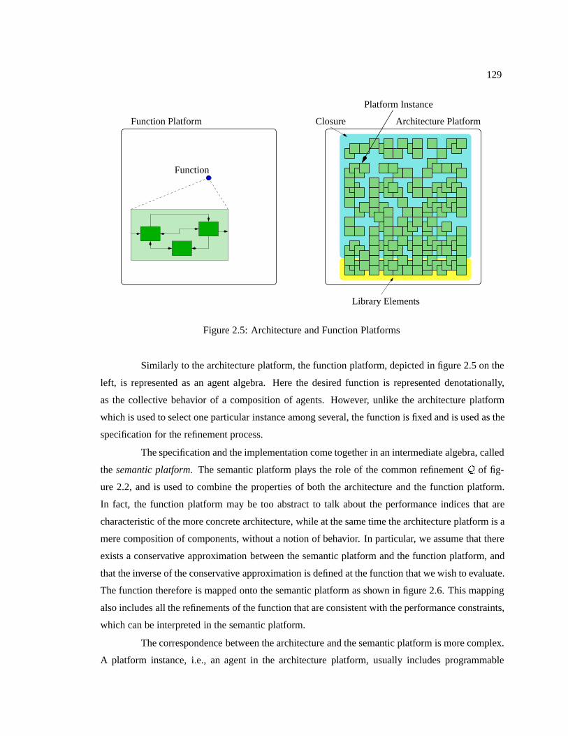
129

Library Elements

Platform Instance

Architecture PlatformFunction Platform

Function

Closure

Figure 2.5: Architecture and Function Platforms

Similarly to the architecture platform, the function platform, depicted in figure 2.5 on the

left, is represented as an agent algebra. Here the desired function is represented denotationally,

as the collective behavior of a composition of agents. However, unlike the architecture platform

which is used to select one particular instance among several, the function is fixed and is used as the

specification for the refinement process.

The specification and the implementation come together in an intermediate algebra, called

the semantic platform. The semantic platform plays the role of the common refinementQ of fig-

ure 2.2, and is used to combine the properties of both the architecture and the function platform.

In fact, the function platform may be too abstract to talk about the performance indices that are

characteristic of the more concrete architecture, while at the same time the architecture platform is a

mere composition of components, without a notion of behavior. In particular, we assume that there

exists a conservative approximation between the semantic platform and the function platform, and

that the inverse of the conservative approximation is defined at the function that we wish to evaluate.

The function therefore is mapped onto the semantic platform as shown in figure 2.6. This mapping

also includes all the refinements of the function that are consistent with the performance constraints,

which can be interpreted in the semantic platform.

The correspondence between the architecture and the semantic platform is more complex.

A platform instance, i.e., an agent in the architecture platform, usually includes programmable

130

Platform Realizations Library Elements

Platform Instance

Architecture PlatformSemantic Platform

Admissible Refinements

Mapped Instance

Function Space

Function

Closure

Figure 2.6: Mapping of function and architecture

elements (microprocessors, programmable logic) that may be customized for the particular function

required. Therefore, each platform instance may be used to implement a variety of functions, or

behaviors. Each of these functions is in turn represented as one agent in the semantic platform. A

platform instance is therefore projected onto the semantic platform by considering the collection of

the agents that can be implemented by the particular instance. These, too, can be organized as a

refinement hierarchy, since the same function could be implemented using different algorithms and

employing different resources even within a particular platform instance. Note that the projection

of the platform instance onto the semantic platform, represented by the rays that originate from the

architecture platform in figure 2.6, may or may not have a greatest element. If it does, the greatest

element represents the non-deterministic choice of any of the functions that are implementable by

the architecture.

An architecture and a function platform may be related using different semantic plat-

forms, and under different notions of refinement. The choice of semantic platform is particularly

important. The agents in the semantic platform must in fact be detailed enough to represent the per-

formance values of interest in choosing a particular platform instance, and a particular realization

(via programmability) of the instance. However, if the semantic platform is too detailed, the corre-

spondence between the platform instance and its realizations may be impractical to compute. This

correspondence is therefore usually obtained by estimation techniques, rather than by analytical

methods.

The semantic platform is partitioned into four different areas. We are interested in the

area that corresponds to the intersection of the refinements of the function and of the functions

131

that are implementable by the platform instance. This area is marked “Admissible Refinements” in

figure 2.6. In fact, the agents that refine the function, but do not refine the architecture, are possible

implementations that are not supported by the platform instance. The agents that refine the platform

instance, but not the function, are possible behaviors of the architecture that are either inconsistent

with the function (they do something else), or they do not meet the performance constraints. The

rest of the agents that are not in the image of any of the maps correspond to behaviors that are

inconsistent with the function and are not implementable by the chosen platform instance.

Among all the possible implementations, one must be chosen as the function to be used

for the next refinement step. Each of the admissible refinements encodes a particular mapping of

the components of the function onto the services offered by the selected platform instance. Of all

those agents, we are usually interested in the ones that are closer to the greatest element, as those

implementations more likely offer the most flexibility when the same refinement process is iterated

to descend to an even more concrete level of abstraction. In addition, several different platform

instances may be considered to search among the different topologies and available resources and

services.

Once a suitable implementation has been chosen, the process continues with the next

refinement step. The new function platform is obtained as the combination of the semantic platform

that provides information on the desired behavior, and the architecture platform, which provides

information on the topology and the structure of the mapped implementation. The new function

is then mapped to a new architecture, employing the same device of a semantic platform as an

intermediate domain.

132

Chapter 3

Conformance, Mirrors and Local

Specification Synthesis

This chapter is devote to studying the problem of refinement verification in general, and

the problem of local specification synthesis in particular. The techniques that we present here are a

generalization to agent algebras of the corresponding concepts introduced by Dill for asynchronous

trace structures [34]. By abstracting the notion of an agent, our definitions are based on more

fundamental properties of models of computation. Our results therefore provide more insights on the

interplay between the ordering on the agents, the notion of compatibility and its maximal elements.

In this chapter we show that the order of an agent algebra can often be characterized in

terms of substitutability as aconformance relation. We introduce the definition of a conformance

order by considering the effect of substituting an agent for another agent in every possible con-

text. We parameterize the notion of substitutability using a set of agents, called aconformance set.

Conformance can be used to verify the order relationship between agents. In this chapter we also

introduce the notion of themirror of an agent, which, together with a conformance order, reduces

the task of refinement verification to computing a parallel composition and checking membership

with the conformance set. The relationship between mirrors and conservative approximations is

also illustrated here.

The conformance order and the mirror function are used in agent algebras to formulate

and to solve the problem of synthesizing a local specification subject to a context. This construction,

which is independent of the particular agent algebra considered, is useful in developing synthesis

techniques, as already discussed in section 1.3. The solution to the problem requires that the context

133

expression be presented in a particular normal form. We show that under certain conditions every

expression can be transformed into an equivalent expression in this form. The normal form is

useful to deal with systems specified as complex interaction of hierarchies, as it allows flattening

the system to a single parallel composition. The normal form is also important for obtaining closed

form solutions to equations involving expressions on agents.

3.1 Expression Equivalence and Normal Forms

In this section we define what it means for two agent expressions to be equivalent and

prove that every expression can be transformed into an equivalent expression in a specific (normal)

form.

We say that two expressions are equivalent if they have the same value for all possible

assignments.

Definition 3.1 (Expression Equivalence). Let Q be an agent algebra. Two expressionsE1 and

E2 overQ are equivalent, writtenE1 � E2, if and only if for all assignments�, [[ E1 ]]� =

[[ E2 ]]�.

In particular the above definition implies that if two expressions are equivalent then they

are defined or undefined for exactly the same assignments. Notice also that because equivalence

depends on the evaluation of the expression, two expressions may be equivalent relative to one agent

algebra and not equivalent relative to another agent algebra. In other words, expression equivalence

depends on the particular choice of underlying agent algebra.

Sometimes it is convenient to consider only a subset of the possible assignments. In that

case we talk about equivalence modulo a set of assignments�0.

Definition 3.2 (Expression Equivalence modulo �0). Let �0 be a set of assignments. Two ex-

pressionsE1 andE2 are equivalent modulo�0, written E1 ��0 E2, if and only if for all

assignments� 2 �0, [[ E1 ]]� = [[ E2 ]]�.

We state the following results for expression equivalence only, but they extend to expres-

sion equivalence modulo�0 in a straightforward way.

Lemma 3.3. Expression equivalence is an equivalence relation.

Because the semantics of expressions is syntax directed, the value of an expression de-

pends only on the value of its subexpressions. Hence

134

Theorem 3.4. Expression equivalence is a congruence with respect to the operators of the agent

algebra.

Proof: We show that ifE1 andE2 are two agent expressions such thatE1 � E2, then for all

alphabetsB, proj(B)(E1) � proj(B)(E2). The cases forrenameandk are similar. The

proof consists of the following series of implications:

E1 � E2

by definition 3.1

, for all assignments�, [[ E1 ]]� = [[ E2 ]]�

) for all assignments�, proj(B)([[ E1 ]]�) = proj(B)([[ E2 ]]�)

by definition 2.46

, for all assignments�, [[ proj(B)(E1) ]]� = [[ proj(B)(E2) ]]�

by definition 3.1

, proj(B)(E1) � proj(B)(E2)

Lemma 3.5. LetE be an agent expression and letE be a subexpression ofE. If E � E0 for some

E0, thenE � E0, whereE0 is obtained fromE by replacingE with E0.

Proof: The proof is by induction on the structure ofE.

Equivalence is useful when we need to transform an expression into a form that is con-

venient for certain applications. In that case, we want to make sure that the transformations do not

change the meaning (the semantics) of the expression. In this work we are particularly interested in

a form where rename operator is applied first, then followed by the parallel composition operator,

and finally by the projection operator. We call this the RCP normal form.

Definition 3.6 (RCP Normal Form). LetQ be an agent algebra and letE0 be the set of expressions:

E0 = f p : p 2 Q:Dg [ f v : v 2 V g:

An agent expressionE is said to be in RCP (i.e., rename, compose, project) normal form if it

is of the form

E = proj(A)(rename(r1)(E1) k � � � k rename(rn)(En))

135

whereA is an alphabet,r1; : : : ; rn are renaming functions andE1; : : : ; En are expressions in

E0.

The RCP normal form is similar to the normal form Dill defined for circuit algebra expres-

sions [33]. In our case, however, we have extended the definition to expressions involving variables.

This normal form corresponds to flattening the hierarchy: all agents are first instantiated using the

rename operator, and are subsequently composed in parallel to form the entire system. The final

projection is used to hide the internal signals.

Other normal forms are also possible. In the rest of this section we will however con-

centrate on the RCP normal form, since we will need it to solve inequalities for variables in the

application shown in section 3.4. In particular, we are interested in sufficient conditions that an

algebra must satisfy in order for all expressions to have an equivalent RCP normal form. We will

approach this problem in steps of increasing complexity. First we will consider expressions that

do not involve variables, i.e., closed expressions. In that case, the expression is either defined or

undefined, a condition that greatly simplifies the search for the normal form. As a second step, we

will consider expressions where variables can only be assigned agents with a specific alphabet and

that always make the expression defined or not defined. This is a case that is interesting in practice,

and that does not require the stronger conditions of the general result. Finally we will explore a set

of restrictions that are needed to obtain an equivalent normal form in the general case. We will see

that alphabets again play a major role, and that they must be restricted in order for the appropri-

ate renaming functions and projection operators to exist. All of this is formalized in the following

definitions and results.

Definition 3.7 (Closed-Normalizable Agent Algebra). Let Q be an agent algebra. We say that

Q is a closed-normalizable agent algebra if the renaming, projection parallel composition

operators satisfy the axioms given below, wherep andp0 are elements ofD andA = �(p)

andA0 = �(p0).

A8. If rename(r)(p) is defined, then it is equal torename(r jA!r(A))(p).

A9. rename(r0)(rename(r)(p)) = rename(r0 Æ r)(p), if the left hand side of the equation

is defined.

A10. If proj(B)(p) is defined, then it is equal toproj(B \A)(p).

A11. proj(B)(proj(B0)(p)) = proj(B \ B0)(p), if the left hand side of the equation is

defined.

136

A12. If rename(r)(proj(B)(p)) is defined, then there exists a functionr0 such that

rename(r)(proj(B)(p)) = proj(r0(B))(rename(r0)(p)):

A13. If proj(B)(p) is defined, then there exists a functionr such thatr(A) \A0 � B and

proj(B)(p) = proj(B)(rename(r)(p)):

A14. rename(r)(pkp0) = rename(r jA!r(A))(p)k rename(r jA0!r(A0))(p0), if the left hand

side of the equation is defined.

A15. proj(B)(p k p0) = proj(B \A)(p) k proj(B \A0)(p0), if (A \A0) � B.

The axioms formalize certain assumptions regarding the semantic domain. In particular

they formalize the intuition that the renaming operator should only depend on the value of the

renaming function for the signals actually used by the argument, and that consecutive applications of

the renaming operator are equivalent to a single application with the appropriate renaming function.

Similar consideration apply for projection. A12 states that rename and projection commute when

the retained set and the renaming function are changed appropriately. Also, A14 states that rename

commutes with parallel composition, and A15 states a similar property for projection. Note that

projection commutes with parallel composition only if the common signals between the agents being

composed are retained after the composition. This is necessary, or else the expression on the right

hand side of the equation would lack the necessary information to compute the full synchronization

between the agents. Finally, A13 asserts that it is possible to arbitrarily rename the signals of an

agent that are not retained in a projection. This is essential to avoid conflicts of names when applying

A15 from right to left, in order to make the “local” signals of each of the agents unique.

The axioms can be used to algebraically transform an expression into an equivalent RCP

normal form, as the next result shows. Technically, since we are considering only sufficient and not

necessary conditions, the termnormalizable should apply to all agent algebras whose expression

can be put in RCP normal form, whether or not they satisfy the axioms. In practice, we restrict

our attention to only algebras that do satisfy the axioms for the purpose of normalization, and we

therefore use the term to distinguish them from those that do not. We will continue to use this

convention for the rest of this document, including the more general cases of normalizable agent

algebras.

Theorem 3.8 (Normal Form - Closed Expressions). LetQ be a closed-normalizable agent alge-

bra, and letE be a closed expression overQ. ThenE is equivalent to an expression in RCP

normal form.

137

Proof: Let E be a closed expression. IfE is undefined, thenE is equivalent to any undefined

closed expression in RCP normal form. IfE is defined, then we construct an equivalent

closed expression in RCP normal form by induction on the structure of expressions.

� AssumeE = p for some agentp 2 Q:D. ThenE = proj(A)(rename(idA)(p)) by A4

and A2.

� AssumeE = proj(B)(E1). Then, by induction,E1 is equivalent to an expression

E01 = proj(B0)(rename(r1)(p1) k � � � k rename(rn)(pn)) in RCP normal form. Then

E = proj(B)(proj(B0)(rename(r1)(p1) k � � � k rename(rn)(pn)))

By A11

= proj(B \B0)(rename(r1)(p1) k � � � k rename(rn)(pn))

which is in RCP normal form.

� AssumeE = rename(r)(E1). Then, by induction,E1 is equivalent to an expression

E01 = proj(B)(rename(r1)(p1) k � � � k rename(rn)(pn)) in RCP normal form. Then

E = rename(r)(proj(B)(rename(r1)(p1) k � � � k rename(rn)(pn)))

By A12 there exists a renaming functionr0 such that

= proj(r0(B))(rename(r0)(rename(r1)(p1) k � � � k rename(rn)(pn)))

By A6, A14 and A3

= proj(r0(B))(rename(r0 jr1(A1)!r0(r1(A1)))(rename(r1)(p1)) k � � �

k rename(r0 jrn(An)!r0(rn(An)))(rename(rn)(pn)))

By A9

= proj(r0(B))(rename(r0 jr1(A1)!r0(r1(A1))Æ r1)(p1) k � � �

k rename(r0 jrn(An)!r0(rn(An))Æ rn)(pn))

which is in RCP normal form.

� AssumeE = E1 k E2. Then, by induction,E1 is equivalent to an RCP normal form

E01 = proj(B1)(rename(r11)(p11) k � � � k rename(rn1)(pn1)) andE2 is equivalent to

an RCP normal formE02 = proj(B2)(rename(r12)(p12)k � � � k rename(rn2)(pn2)). Let

A1 be the alphabet of expressionE001 such thatE01 = proj(B1)(E001 ). We can assume,

138

without loss of generality, thatB1 � A1 andB2 � A2. By A13 there exists a function

r1 such thatr1(A1) \A2 � B1 and

proj(B1)(E001 ) = proj(B1)(rename(r1)(E001 )):

Similarly, there exists a functionr2 such thatr2(A2) \ (A1 [ r1(A1)) � B2 and

proj(B2)(E002 ) = proj(B2)(rename(r2)(E002 )):

By A10

proj(B1)(E001 ) = proj(B1 \ r1(A1))(rename(r1)(E

001 ))

proj(B2)(E002 ) = proj(B2 \ r2(A2))(rename(r2)(E002 ))

Note that sincer1(A1)\A2 � B1, and sinceB2 � A2, alsor1(A1)\B2 � B1. Thus

alsor1(A1) \B2 � B1 \ r1(A1). Hence

(B1 [B2) \ r1(A1) = (B1 \ r1(A1)) [ (B2 \ r1(A1)) = B1 \ r1(A1):

Likewise, sincer2(A2) \ (A1 [ r1(A1)) � B2, alsor2(A2) \ A1 � B2 and therefore

r2(A2) \B1 � B2. Thusr2(A2) \B1 � B2 \ r2(A2). Hence

(B1 [B2) \ r2(A2) = (B1 \ r2(A2)) [ (B2 \ r2(A2)) = B2 \ r2(A2):

Thus we have

proj(B1)(E001 ) = proj((B1 [B2) \ r1(A1))(rename(r1)(E001 ))

proj(B2)(E002 ) = proj((B1 [B2) \ r2(A2))(rename(r2)(E

002 ))

Moreover, sincer2(A2) \ (A1 [ r1(A1)) � B2, we also haver2(A2) \ r1(A1) � B2,

so thatr2(A2) \ r1(A1) � B1 [B2. Hence by A15

proj(B1)(E001 ) k proj(B2)(E

002 ) =

= proj((B1 [B2) \ r1(A1))(rename(r1)(E001 )) k

proj((B1 [B2) \ r2(A2))(rename(r2)(E002 ))

= proj(B1 [B2)(rename(r1)(E001 ) k rename(r2)(E002 ))

139

By A9 and A6

rename(r1)(E001 ) = rename(r1 Æ r11)(p11) k � � � k rename(r1 Æ rn1(pn1)

rename(r2)(E002 ) = rename(r2 Æ r12)(p12) k � � � k rename(r2 Æ rn2(pn2)

which proves the result.

If we consider an expression that involves variables, the axioms of agent algebras and the

axioms of definition 3.7 may not be sufficient to ensure the existence of an equivalent normal form.

Consider, for example, the expression

E = v:

We must find a renaming functionr and an alphabetB such that

E � proj(B)(rename(r)(v)):

The axioms are insufficient for two reasons. In the first place, A4 and A2 ensure the existence of an

appropriate renaming functionr and alphabetB for each agent. However, the algebra must be such

thatthe same renaming functionr and alphabetB can be used to construct an equivalent expression

for all agents (or, at least, for the subset of agents that are assigned tov). The same is true of all

the axioms that for all agents dictate the existence of a certain renaming function or alphabet. To

make the algebra normalizable, the order of the quantifiers of these axioms must be exchanged, thus

strengthening the requirements.

Secondly, we have dealt with the problem of definedness in theorem 3.8 by deriving a

different normal form, according to whether the original closed expression is defined or not. How-

ever, unlike a closed expression, an expression may be defined or not defined depending on the

assignment to its variables. To ensure equivalence, we must find an expression in normal form that

is defined and not defined for exactly the same assignments. In the particular case above, since the

expressionE = v is defined for all possible assignments tov, we must find a renaming functionr

and an alphabetB such thatproj(B)(rename(r)(v)) is also always defined. Consequently, we must

strengthen the axioms in two ways: by first requiring that the equalities that occur in the axioms are

valid whether or not the left hand side is defined; and by introducing additional assumptions on the

definedness of the operators to ensure the existence of the normal form.

140

However, one case that requires minimal strengthening of the axioms, and that is of great

practical interest, is when variables are always assigned agents with the same alphabet, and such

that the expression is always defined or always not defined. This is, for instance, the case in [33].

Definition 3.9 (Alpha-Normalizable Agent Algebra). Let Q be a normalizable agent algebra.

We say thatQ is alpha-normalizable if the renaming, projection and parallel composition

operators satisfy the following axioms:

A16. For all alphabetsA there exists a renaming functionr0 such that for all agentsp such

that�(p) = A, if rename(r)(proj(B)(p)) is defined, then

rename(r)(proj(B)(p)) = proj(r0(B))(rename(r0)(p)):

A17. For all alphabetsA there exists a renaming functionr such that for all agentsp such

that�(p) = A, if proj(B)(p) is defined, thenr(A) \A0 � B and

proj(B)(p) = proj(B)(rename(r)(p)):

Note that, as in definition 3.7, the axioms are stated directly in terms of the operators and

the agents of the algebra. However, by theorem 3.4, they can be used with expressions whenever

every evaluation (possibly restricted to a set of assignments�0) of the expressions involved satisfies

the requirements of the axiom. In that case, the equality must be replaced by equivalence (possibly

modulo�0). This remark applies especially to the proofs of theorem 3.10 and theorem 3.16 below.

Theorem 3.10 (Normal Form - Same Alphabet). LetQ be an alpha-normalizable agent algebra.

LetE be an expression overQ and let�0 be a set of assignments such that for all�1; �2 2 �0,

[[ E ]]�1# if and only if [[ E ]]�2# and for all variablesv, �(�1(v)) = �(�2(v)). ThenE is

equivalent modulo�0 to an expressionE0 in RCP normal form.

Proof: The proof is similar to the proof of theorem 3.8. In fact, the transformations in the induction

are the same and equally valid for every assignment (subject to the restrictions set forth in the

statement of the theorem) and therefore preserve the evaluation of the expression no matter

what agents replaces the variables.

In general, an equivalent RCP normal form for an expression that involves unrestricted

variables and quantities does not exist. To see why, consider the following expressionE:

E = proj(B)(p) k v:

141

To normalize this expression we must renamep so that the signals that are in its alphabet and that

are not inB do not conflict with the signals inv. The alphabet ofv however depends on its assigned

value. Thus, if we assume that for each signal in the master alphabetQ:A there is an agent that

has that signal in its alphabet, then there exists no renaming function with the above property. One

could avoid conflicts by renamingv by folding the master alphabet into a subset of itself (this can be

done only if the master alphabet is infinite), thus making the extra signals available forp. However,

in general this changes the meaning of the expression (sincev now appears renamed without being

guarded by a projection), thus making it difficult to obtain an equivalent expression.

One could of course require that projection and parallel composition always commute.

That, however, would not only unduly restrict the kinds of models of computation that can be

studied as agent algebras, but, more importantly, would be contrary to the intuitive interpretation

of the operations. Therefore, in the absence of conditions specific to particular agent algebras, we

must restrict the extent of the alphabets that are used in the expression and in the assignments to the

variables.

In the rest of this section we present sufficient conditions for the existence of an equivalent

RCP normal form for expressions involving variables. In particular, we are looking for restrictions

on the alphabet of agents while still maintaining full generality. This can be achieved by restricting

the use of the master alphabet to only a subset of the available signals, as long as the subset has

the same cardinality as the whole and still leaves enough signals available for the operations of

renaming. As a consequence, the equivalence will be modulo some set of assignments�0 that

satisfies the restrictions.

In what follows we will make use of the following lemmas and definitions.

Lemma 3.11. LetQ be an agent algebra. LetE1 andE2 be two expression overQ and�0 a set of

assignments such thatE1 ��0 E2. Then�([[ E1 ]]�0) = �([[ E2 ]]�0).

Proof: Let a 2 �([[ E1 ]]�0). Then there exists an assignment� 2 �0 such that [[E1 ]]� = p and

a 2 �(p). But sinceE1 ��0 E2, then also [[E2 ]]� = p. Thereforea 2 �([[ E2 ]]�0). The

reverse direction is similar.

Definition 3.12 (Small Subset). Let W be a set and letB be a subset ofW . We say thatB is a

small subset ofW , writtenB bW , if:

� W is infinite.

142

� The cardinality of the complementW �B is greater than or equal to the cardinality of

B.

Lemma 3.13. LetX andZ be sets such thatX b Z. Then there exists a setY such thatX b Y b

Z.

Proof: Let Y1 andY2 be two subsets ofZ �X of the same size such thatZ �X = Y1 [ Y2, and

let Y = X [ Y1. SinceZ �X is infinite, jY1j = jY2j = jZ �Xj. SincejZ �Xj � jXj, also

jY1j � jXj. ThereforeX b Y .

SinceX b Y , jXj � jY1j. Therefore, sinceY = X [ Y1, jY j = jY1j. Therefore

alsojY2j = jY j. HenceY b Y [ Y2 = Z.

We now have the vocabulary to state and prove the main result of this section.

Definition 3.14 (Normalizable Agent Algebra). Let Q be an agent algebra. We say thatQ is

a normalizable agent algebra if the renaming, projection and parallel composition operators

satisfy the following axioms:

A18. For all alphabetsA there exists an alphabetB such thatA � B and for all agentsp

such that�(p) � A

p = rename(idB)(p):

A19. For all alphabetsB and agentsp and for all alphabetsA0 such that�(p) \A0 = ;

proj(B)(p) = proj(B [A0)(p):

A20. For all alphabetsB andB0, and for all agentsp

proj(B)(proj(B0)(p)) = proj(B \B0)(p):

A21. For all renaming functionsr1 andr2 and for all agentsp

rename(r1)(rename(r2)(p)) = rename(r1 Æ r2)(p)

where for all signalsa,

(r1 Æ r2)(a) =

8<:

r1(r2(a)) if r1(r2(a))#

" otherwise.

143

A22. For all renaming functionsr and for all alphabetsB there exist renaming functionsr0

andr00 such that for all agentsp

rename(r)(proj(B)(p)) = proj(r0(B))(rename(r00)(p)):

A23. For all alphabetsB, for all alphabetsA and for all alphabetsA0 such thatj(Q:A �

A0)�Bj � jA�Bj there exists a renaming functionr such thatr(A)\A0 � B and

for all agentsp such that�(p) � A

proj(B)(p) = proj(B)(rename(r)(p)):

A24. For all renaming functionsr and for all agentsp1 andp2

rename(r)(p1 k p2) = rename(r)(p1) k rename(r)(p2):

A25. For all alphabetsB and for all agentsp1 andp2 such that�(p1) \ �(p2) � B

proj(B)(p1 k p2) = proj(B)(p1) k proj(B)(p2):

The axioms of normalizable agent algebras are essentially equivalent to those of defi-

nition 3.7 for closed-normalizable algebras. They differ in the way alphabets and variables are

handled.

It is easy to show that A19 is equivalent to a similar form that involves restricting the

retained alphabet, rather than extending it.

Lemma 3.15. LetQ be a normalizable agent algebra. Then the following two statements are equiv-

alent.

1. Q satisfies A19, i.e., for all alphabetsB and agentsp and for all alphabetsA0 such that

�(p) \A0 = ;

proj(B)(p) = proj(B [A0)(p):

2. for all alphabetsB and agentsp and for all alphabetsA0 such that�(p) � A0

proj(B)(p) = proj(B \A0)(p):

144

Proof: For the forward implication, assume item 1 is true. LetB be an alphabet,p an agent andA0

an alphabet such that�(p) � A0. LetK = B \A0 andJ 0 = B �A0. Then

�(p) � A0

sinceJ 0 \A0 = ;

, �(p) \ J 0 = ;

by item 1

) proj(K)(p) = proj(K [ J 0)(p)

, proj(B \A0)(p) = proj((B \A0) [ (B �A0))(p)

, proj(B \A0)(p) = proj(B)(p)

For the reverse implication, assume item 2 is true. LetB be an alphabet,p an agent andA0

an alphabet such that�(p) \A0 = ;. LetK = B [A0 andJ 0 = �(p) [B. Then

�(p) � J 0

by item 2

) proj(K)(p) = proj(K \ J 0)(p)

, proj(B [A0)(p) = proj((B [A0) \ (�(p) [B))(p)

, proj(B [A0)(p) = proj((B \ �(p)) [ (B \B) [ (A0 \ �(p)) [ (A0 \B))(p)

sinceB \ �(p) � B,A0 \ �(p) = ; andA0 \B � B

, proj(B [A0)(p) = proj(B)(p)

The following theorem shows that in a normalizable agent algebra any expression can be

turned into an equivalent expression in RCP normal form when enough signals are available. The

notation is simpler if we assume that the expression does not contain constants. This assumption is

without loss of generality, since the case when an expression contains constants can be obtained by

representing the constants with unique variables and by considering only assignments that assign

the corresponding constant to the variables.

Theorem 3.16 (Normal Form). Let Q be an agent algebra such thatQ:A is infinite, and letE

be an expression overQ that does not involve constants. Let�0 be a set of assignments and

W � Q:A be an alphabet such that�([[ sub(E) ]]�0) bW . ThenE is equivalent modulo�0

145

to an expressionE0 in RCP normal form such that�([[ sub(E0) ]]�0) � W . In addition, if a

variablev appearsk times inE, then it appearsk times inE0.

Proof: The proof uses the following result.

Lemma 3.17. Let E = rename(r1)(v1) k � � � k rename(rn)(vn) be an expression such that

�([[ E ]]�0) = A. Then

rename(r)(E) ��0 rename(r Æ r1)(v1) k � � � k rename(r Æ rn)(vn)

and both�([[ rename(r)(E) ]]�0) = r(A) and for alli, �([[ rename(r Æ ri)(vi) ]]�0) �

r(A).

Proof: By A6 and A24

rename(r)(E) ��0 rename(r)(rename(r1)(v1))k� � �krename(r)(rename(rn)(vn));

and by A21

rename(r)(E) ��0 rename(r Æ r1)(v1) k � � � k rename(r Æ rn)(vn):

Since�([[ E ]]�0) = A, and by A5, for alli, �([[ rename(ri)(vi) ]]�0) � A. Therefore

by A3, �([[ rename(r)(E) ]]�0) = r(A) and for all i, �([[ rename(r Æ ri)(vi) ]]�0) �

r(A).

The proof is by induction on the structure of expressions.

� LetE = v. LetA = �([[ E ]]�0). By A18 there exists an alphabetB such thatA � B

and for allp such that�(p) � A

p = rename(idB)(p):

146

Let now� 2 �0 be an assignment. Then by definition 2.46

[[ v ]]� = �(v)

Since�(�(v)) � A

= rename(idB)(�(v))

by A2, since�(�(v)) = �(rename(idB)(�(v)))

= proj(�(�(v)))(rename(idB)(�(v)))

by A19, since�(�(v)) \A � �(�(v))

= proj(A)(rename(idB)(�(v)))

by definition 2.46

= [[ proj(A)(rename(idB)(v)) ]]�:

Thus by definition 3.2

v ��0 proj(A)(rename(idB)(v)) = E0

which is in RCP normal form.

By inspection

sub(E0) = f v; rename(idB)(v);proj(A)(rename(idB)(v))g:

By hypothesis,

�([[ v ]]�0) = A �W:

Sincev ��0 rename(idB)(v), by lemma 3.11

�([[ rename(idB)(v) ]]�0) = A �W:

Sincev ��0 proj(A)(rename(idB)(v)), by lemma 3.11

�([[ proj(A)(rename(idB)(v)) ]]�0) = A �W:

Therefore,�([[ sub(E0) ]]�0) �W .

By inspection, if a variablev appearsk times inE, it appearsk times in the normal

form.

147

� LetE = proj(B)(E1). By hypothesis,�([[ sub(E) ]]�0) bW . Then, sincesub(E1) �

sub(E), also�([[ sub(E1) ]]�0) bW . Then, by induction hypothesis,E1 is equivalent

to an expressionE01 in RCP normal form

E01 = proj(B0)(rename(r1)(v1) k � � � k rename(rn)(vn))

and�([[ sub(E01) ]]�0) �W . Then by theorem 3.4

E ��0 proj(B)(proj(B0)(rename(r1)(v1) k � � � k rename(rn)(vn))):

By A20,E is equivalent modulo�0 to an expressionE0

E ��0 E0 = proj(B \B0)(rename(r1)(v1) k � � � k rename(rn)(vn))

which is in RCP normal form.

Let

E001 = rename(r1)(v1) k � � � k rename(rn)(vn):

Then

sub(E0) = fE0g [ sub(E001 ):

Since by hypothesis�([[ E ]]�0) �W , and sinceE ��0 E0, by lemma 3.11

�([[ E0 ]]�0) �W:

Sincesub(E001 ) � sub(E01), and since�([[ E01 ]]�0) �W ,

�([[ sub(E001 ) ]]�0) �W:

Therefore,�([[ sub(E0) ]]�0) �W .

In addition, if a variablev appearsk times inE, it appearsk times inE1, and therefore,

by induction, it appearsk times inE01 and in the final normal form.

� Let E = rename(r)(E1). By hypothesis,�([[ sub(E) ]]�0) b W . Then, since clearly

sub(E1) � sub(E), also�([[ sub(E1) ]]�0) b W . Then by inductionE1 is equivalent

to an expressionE01 in RCP normal form

E01 = proj(B0)(rename(r1)(v1) k � � � k rename(rn)(vn))

148

and�([[ sub(E01) ]]�0) �W .

LetE001 = rename(r1)(v1) k � � � k rename(rn)(vn). Then, by theorem 3.4

E ��0 rename(r)(proj(B0)(E001 )):

By A22 there exist renaming functionr0 andr00 such that

E ��0 proj(r0(B0))(rename(r00)(E001 )):

Let nowA = �([[ rename(r00)(E001 ) ]]�0) andB = r0(B0)\A. Since�([[ E ]]�0) bW ,

by A1 and lemma 3.11 alsoB bW . By lemma 3.15

E ��0 proj(B)(rename(r00)(E001 )):

Let nowA0 = Q:A�W . Then(Q:A�A0)�B =W �B. Note thatr00 is a bijection,

and for any assignment� 2 �0, if [[ rename(r00)(E001 ) ]]� is defined then also [[E001 ]]�

is defined. Thus, since�([[ E001 ]]�0) � W , jAj = j�([[ rename(r00)(E001 ) ]]�0)j �

j�([[ E001 ]]�0)j � jW j. Hence, sinceB � W andB � A, jW � Bj � jA � Bj.

Therefore, by A23 there exists a renaming functionr000 such thatr000(A) \A0 � B and

E ��0 proj(B)(rename(r000)(rename(r00)(E001 ))):

By A21

E ��0 proj(B)(rename(r000 Æ r00)(E001 )):

By lemma 3.17

E ��0 E0 = proj(r0(B))(rename(r000Ær00 Ær1)(v1)k� � � krename(r000Ær00 Ærn)(vn))

which is in RCP normal form.

By inspection

sub(E0) = f v1; : : : ; vng [

= [ f rename(r000 Æ r00 Æ r1)(v1); : : : ; rename(r000 Æ r00 Æ rn)(vn)g [

= [ f rename(r000 Æ r00 Æ r1)(v1) k � � � k rename(r000 Æ r00 Æ rn)(vn)g [

= [ fE0g

149

Since for alli, vi 2 sub(E01), and since�([[ sub(E01) ]]�0) �W ,

�([[ f v1; : : : ; vng ]]�0) �W:

Note thatr000(A) \A0 � B impliesr000(A) �W . Therefore, by lemma 3.17,

�([[ f rename(r000 Æ r00 Æ r1)(v1); : : : ; rename(r000 Æ r00 Æ rn)(vn)g ]]�0) � r000(A)

� W;

and

�([[ rename(r000 Æ r00 Æ r1)(v1) k � � � k rename(r000 Æ r00 Æ rn)(vn) ]]�0) � r000(A)

� W:

Since by hypothesis�([[ E ]]�0) �W , and sinceE ��0 E0, by lemma 3.11,

�([[ E0 ]]�0) �W:

Therefore,�([[ sub(E0) ]]�0) �W .

In addition, if a variablev appearsk times inE, it appearsk times inE1, and therefore,

by induction, it appearsk times inE01 and in the final normal form.

� LetE = E1 kE2.

LetA = �([[ E ]]�0).

Since by hypothesisA b W , by lemma 3.13, there exists an alphabetX such that

A b X andX bW .

Then, sincesub(E1) � sub(E) andsub(E2) � sub(E), also�([[ E1 ]]�0) b X and

�([[ E2 ]]�0) b X. Then, by induction,E1 andE2 are equivalent to expressionsE01 and

E02 in RCP normal form

E01 = proj(B01)(rename(r1;1)(v1;1) k � � � k rename(r1;n)(v1;n))

E02 = proj(B02)(rename(r2;1)(v2;1) k � � � k rename(r2;m)(v2;m))

and�([[ sub(E01) ]]�0) � X and�([[ sub(E02) ]]�0) � X.

150

Let

E001 = rename(r1;1)(v1;1) k � � � k rename(r1;n)(v1;n)

A001 = �([[ E001 ]]�0)

B1 = B01 \A001

E002 = rename(r2;1)(v2;1) k � � � k rename(r2;m)(v2;m)

A002 = �([[ E001 ]]�0)

B2 = B02 \A002

Then by theorem 3.4 and lemma 3.15

E01 ��0 proj(B1)(E001 )

E02 ��0 proj(B2)(E002 )

SinceX b W , by lemma 3.13 there exists an alphabetY such thatX b Y and

Y bW .

LetA01 = Q:A � (W � Y ) andA02 = Q:A � (Y �X). Clearly sinceX b Y b W

andA001 � X, jW � Y j � jY j � jXj � jA001j. Therefore, sinceB1 � Y , j(Q:A �

A01)�B1j = j(W � Y )�B1j = jW � Y j � jA001 �B1j.

Similarly jY �Xj � jXj � jA002 j. Therefore, sinceB2 � X, j(Q:A � A02) � B2j =

j(Y �X)�B2j = jY �Xj � jA002 �B2j.

Therefore, by A23 there exist renaming functionsr01 andr02 such thatr01(A001) \ A01 �

B1, r02(A002) \A

02 � B2 and

E01 ��0 proj(B1)(rename(r01)(E001 ))

E02 ��0 proj(B2)(rename(r02)(E002 ))

By definition, B2 � X � A01 and�([[ rename(r01)(E001 ) ]]�0) = r01(A

001), therefore

sincer01(A001) \ A01 � B1, alsor01(�([[ rename(r01)(E

001 ) ]]�0)) \ B2 � B1. Similarly,

r02(�([[ rename(r01)(E001 ) ]]�0)) \B1 � B2. Therefore by A19, denotingB = B1 [B2

E01 ��0 proj(B)(rename(r01)(E001 ))

E02 ��0 proj(B)(rename(r02)(E002 ))

151

By the previous definitions,

�([[ rename(r01)(E001 ) ]]�0) � B1 [ (W � Y );

�([[ rename(r02)(E002 ) ]]�0) � B2 [ (Y �X):

In addition, since(W � Y ) \ (Y �X) = ;, (B1 [ (W � Y )) \ (B2 [ (Y �X)) =

B1 \ B2 � B. Hence�([[ rename(r01)(E001 ) ]]�0) \ �([[ rename(r02)(E

002 ) ]]�0) � B.

Therefore, by A25

E ��0 proj(B)(rename(r01)(E001 ) k rename(r02)(E

002 )):

By lemma 3.17

rename(r01)(E001 ) ��0 rename(r01 Æ r1;1)(v1;1) k � � � k rename(r01 Æ r1;n)(v1;n)

rename(r02)(E002 ) ��0 rename(r02 Æ r2;1)(v2;1) k � � � k rename(r02 Æ r2;m)(v2;m):

Therefore by theorem 3.4

E ��0 E0 = proj(B)(rename(r01 Æ r1;1)(v1;1) k � � � k rename(r01 Æ r1;n)(v1;n) k

k rename(r02 Æ r2;1)(v2;1) k � � � k rename(r02 Æ r2;m)(v2;m))

which is in RCP normal form.

By inspection

sub(E0) = f v1;1; : : : ; v1;ng [

= [ f v2;1; : : : ; v2;mg [

= [ f rename(r01 Æ r1;1)(v1;1); : : : ; rename(r02 Æ r2;m)(v2;m)g [

= [ f rename(r01 Æ r1;1)(v1;1) k � � � k rename(r02 Æ r2;m)(v2;m)g [

= [ fE0g

Since for alli, v1;i 2 sub(E01), and since�([[ sub(E01) ]]�0) �W ,

�([[ f v1;1; : : : ; v1;ng ]]�0) �W:

Similarly

�([[ f v2;1; : : : ; v2;mg ]]�0) �W:

152

Note thatr01(A001) \ A01 � B1 implies r01(A

001) � W , sinceQ:A � W � A01 and

B1 � A001 �W . Therefore by lemma 3.17

�([[ f rename(r01 Æ r1;1)(v1;1); : : : ; rename(r01 Æ r1;n)(v1;n)g ]]�0) � r01(A001) �W

�([[ rename(r01 Æ r1;1)(v1;1) k � � � k rename(r01 Æ r1;n)(v1;n) ]]�0) � r01(A001) �W

Similarly

�([[ f rename(r02 Æ r2;1)(v2;1); : : : ; rename(r02 Æ r2;m)(v2;m)g ]]�0) � r02(A002) �W

�([[ rename(r02 Æ r2;1)(v2;1) k � � � k rename(r02 Æ r2;m)(v2;m) ]]�0) � r02(A002) �W

Since by hypothesis�([[ E ]]�0) �W , and sinceE ��0 E0, by lemma 3.11

�([[ E0 ]]�0) �W:

Therefore,�([[ sub(E0) ]]�0) �W .

In addition, assume a variable appearsm times inE. Then it appearsj times inE1 and

k times inE2 such thatm = j + k. By induction, it appearsj times inE01 andk times

in E02, and therefore it appearsj + k times in the final normal form.

The rest of this section is devoted to proving the validity of some of the axioms for a few

examples.

Example 3.18 (Alphabet Algebra). The alphabet agent algebraQ described in example 2.26 is a

normalizable agent algebra. Here we show that A23 is satisfied.

Lemma 3.19. Q satisfies A23.

Proof: Let B, A andA0 be alphabets overQ such thatj(Q:A � A0) � Bj � jA � Bj. Let

r0 : (A�B) 7! (Q:A�A0)�B be any injection fromA�B toQ:A�A0 �B. The

injection exists because of the assumption on the cardinality of the sets. Then define an

injectionr : A 7! Q:A as follows:

r(a) =

8<:

r0(a) if a 2 A�B

idA(a) otherwise

153

Then ifp is an agent such that�(p) � A, and restricting the codomain ofr to r(A),

proj(B)(p) = B \ �(p)

= B \ r(�(p))

= proj(B)(rename(r)(p)):

Therefore A23 is satisfied.

Example 3.20 (IO Agent Algebra). The IO agent algebraQ described in example 2.29 is normal-

izable. Here we show that A25 is satisfied.

Lemma 3.21. Q satisfies A25.

Proof: LetB be an alphabet and letp1 andp2 be two agents such that�(p1) \ �(p2) � B.

Assumeproj(B)(p1 k p2) is defined. Then by definition(I1 [ I2) � (O1 [ O2) � B.

We now show thatI1 � B. Let i 2 I1 be a signal. Then by definitioni 62 O1. Assume

i 62 O2. Theni 2 (I1 [ I2) � (O1 [ O2) and thereforei 2 B. On the other hand,

assumei 2 O2. Theni 2 �(p1) \ �(p2). Thereforei 2 B. HenceI1 � B. Similarly,

I2 � B. Thereforeproj(B)(p1) k proj(B)(p2) is defined. In addition

proj(B)(p1 k p2) = ((I1 [ I2)� (O1 [O2); (O1 [O2) \B)

proj(B)(p1) k proj(B)(p2) = ((I1 [ I2)� ((O1 [O2) \B); (O1 [O2) \B)

Clearly

(I1 [ I2)� (O1 [O2) � (I1 [ I2)� ((O1 [O2) \B):

Let nowi 2 (I1[I2)�((O1[O2)\B). Then eitheri 2 I1 or i 2 I2 (or both). Ifi 2 I1

theni 62 O1 andi 62 O2 \ B. If i 2 O2, theni 2 �(p1) \ �(p2) and thereforei 2 B.

But theni 2 O2 \B, a contradiction. Hencei 62 O2. Theni 2 (I1 [ I2)� (O1 [O2).

Similarly if i 2 I2. Therefore

(I1 [ I2)� ((O1 [O2) \B) = (I1 [ I2)� (O1 [O2)

and

proj(B)(p1 k p2) = proj(B)(p1) k proj(B)(p2):

Assume nowproj(B)(p1 k p2) is not defined. Then there existsi 2 (I1 [

I2)� (O1 [O2) such thati 62 B. But then eitheri 2 I1 or i 2 I2, and therefore either

154

I1 6� B or I2 6� B. Hence eitherproj(B)(p1) or proj(B)(p2) (or both) is undefined.

Thereforeproj(B)(p1) k proj(B)(p2) is undefined.

Example 3.22 (Dill’s IO Agent Algebra). The Dill’s style IO agent algebraQ described in exam-

ple 2.32 is not normalizable. In fact, it does not satisfy A18. The IO agent algebra described

in example 3.20 is a generalization ofQ that is normalizable.

However, Dill’s style IO agent algebra is closed-normalizable. This doesn’t appear

to be a limitation in Dill’s work, since the notion of refinement requires that two agents have

the same sets of inputs and outputs signals. Dill shows that, if assignments to variables are

restricted to assign only certain input and output signals, then the expressions are normaliz-

able [33]. While this is sufficient to prove the results on refinement verification using mirrors,

it is a special case that we need to generalize in our framework.

3.1.1 Construction of Algebras

It is natural to ask whether the constructions introduced in section 2.3 and subsection 2.4.1

preserve the properties of normalization of the expressions. In other words, ifQ1 andQ2 are nor-

malizable agent algebras, is their productQ1 � Q2 and their disjoint sumQ1UQ2 also normaliz-

able?

Clearly, this is the case for disjoint sum, since the resulting agent algebra is simply the

juxtaposition of two agent algebras, that are otherwise unrelated.

Theorem 3.23. LetQ1 andQ2 be normalizable agent algebras. Then their disjoint sumQ1UQ2

is a normalizable agent algebra.

The same is not necessarily true for products. The problem lies in A22 and A23, both of

which demand the existence of renaming functions that make certain equations true.

Take for example A22. SinceQ1 is normalizable, for all renaming functionsr and all

alphabetsB, there exist renaming functionsr01 andr001 such that for all agentsp1 2 Q1:D,

rename(r)(proj(B)(p1)) = proj(r01(B))(rename(r001)(p1)):

Similarly, sinceQ2 is normalizable, there exist renaming functionsr02 andr002 such that for all agents

p2 2 Q2:D,

rename(r)(proj(B)(p2)) = proj(r02(B))(rename(r002)(p2)):

155

In order for the productQ1 � Q2 to be normalizable, there must be renaming functionsr0 andr00

such that for all agentsp = (p1; p2) 2 Q1:D �Q2:D,

rename(r)(proj(B)(p)) = proj(r0(B))(rename(r00)(p)):

But the result follows from the hypothesis only ifr01 = r02 andr001 = r002 , which is not necessarily the

case.

In most practical cases, however, the product of normalizable agent algebras is in fact

normalizable. This is because in practice the renaming operator is defined similarly for different

algebras, given its strong intuitive interpretation. In addition, all other axioms are indeed preserved

by the product, so that only the validity of A22 and A23 must be established.

3.2 Conformance

Let p andp0 be two agents in an ordered agent algebra. Intuitively, if we interpret the order

as refinement, ifp � p0 thenp can be substituted forp0 in every context in whichp0 occurs. If this is

the case we say thatp conforms to p0. In this section we make this notion of substitutability precise.

In our formalization, conformance is parameterized by a set of agentsG, called a conformance set,

and we only require that forp to conform top0, p can be substituted forp0 for all contexts that

evaluate inG. Intuitively, the setG forms an initial partition of the agents. This partition is then

refined by considering the contexts whose evaluation falls in the conformance set. The remaining

contexts, which are of no interest for substitutability, are therefore ignored.

Conformance can be made more general by explicitly considering only a subset of the

possible contexts. We call this notionrelative conformance. In this section we will study these

generalizations, and show the conditions under which relative conformance corresponds to confor-

mance. We are particularly interested in composition contexts, also calledenvironments, which are

limited to the parallel composition with a single agent. Composition contexts will be the basis for

studying mirror functions in the next section.

The concept of the context of an agent in a system plays a central role in the definition of

conformance. It can be formalized using agent expressions.

Definition 3.24 (Expression Context). Let Q be an agent algebra. An expression contextE[�]

overQ is an expression overQ with one free variable.

An expression context may or may not be defined depending on the agent that replaces

156

the free variable. However, the property of>-monotonicity of the operators of an ordered agent

algebra transfers to expression contexts, as well.

Theorem 3.25. LetQ be an ordered agent algebra andp 2 Q:D andp0 2 Q:D be two agents such

thatp � p0. For all expression contextsE[�], if E[p0] is defined thenE[p] is also defined and

E[p] � E[p0].

Proof: The proof is by induction on the structure of the expression context.

� If E[�] = q orE[�] = � then the result follows directly from the hypothesis.

� LetE[�] = rename(r)(E0[�]) and assumeE[p0] is defined. Then alsoE0[p0] is defined.

By induction hypothesisE0[p] is defined andE0[p] � E0[p0]. Sincerename(r)(E0[p0])

is defined andrenameis>-monotonic, thenrename(r)(E0[p]) is defined and

rename(r)(E0[p]) � rename(r)(E0[p0]):

� Let E[�] = proj(B)(E0[�]) and assumeE[p0] is defined. Then alsoE0[p0] is defined.

By induction hypothesisE0[p] is defined andE0[p] � E0[p0]. Sinceproj(B)(E0[p0]) is

defined andproj is>-monotonic, thenproj(B)(E0[p]) is defined and

proj(B)(E0[p]) � proj(B)(E0[p0]):

� LetE[�] = E1[�]kE2[�] and assumeE[p0] is defined. Then alsoE1[p0] andE2[p0] are

defined. By induction hypothesisE1[p] is defined andE1[p] � E1[p0]. Similarly,E2[p]

is defined andE2[p] � E2[p0]. SinceE1[p

0] k E2[p0] is defined andk is>-monotonic,

thenE1[p] k E2[p0] is also defined andE1[p] k E2[p

0] � E1[p0] k E2[p

0]. Similarly we

concludeE1[p] k E2[p] � E1[p] k E2[p0] and therefore since� is transitive

E1[p] kE2[p] � E1[p0] kE2[p

0]:

An ordered agent algebraQ has a conformance order parameterized by a set of agentsG

when the order corresponds to substitutability in the following sense.

Definition 3.26 (Conformance Order). Let Q be an ordered agent algebra and letG be a set of

agents ofQ. We sayQ has aG-conformance order if and only if for all agentsp andp0,

p � p0 if and only if for all expression contextsE, if E[p0] 2 G thenE[p] 2 G.

157

The implication in this definition is strong in the sense that ifE[p0] 2 G, thenE[p] must

be defined (and be a member ofG).

Each set of agentsG induces a particular order, whether or not the algebra has aG-

conformance order.

Definition 3.27. LetQ be an agent algebra and letG be a set of agents ofQ. We defineQ:conf(G)

to be the agent algebra that is identical toQ except that it has aG-conformance order.

We denote the order ofQ:conf(G) with the symbol�G and we say thatG induces the

order�G. In the rest of this section we will study some of the properties ofQ:conf(G). In par-

ticular we are interested in characterizing whenQ:conf(G) is an ordered agent algebra (i.e., the

operators of projection, renaming and parallel composition are>-monotonic) and whenQ has a

G-conformance order,

Lemma 3.28. LetQ be an ordered agent algebra and letG be a subset ofQ:D. Consider the agent

algebrasQ:conf(G) andQ:conf(D). ThenQ:conf(G) is an ordered agent algebra if and

only if for all agentsp andp0,

p �G p0 ) p �D p0:

Proof: To show thatQ:conf(G) is an ordered agent algebra, we need only show that its renaming,

projection and parallel composition operators are>-monotonic relative to its agent ordering.

We prove the projection case (the others are similar).

Let p andp0 be two agents such thatp �G p0. We must show that ifproj(B)(p0) is

defined, thenproj(B)(p) is defined, andproj(B)(p) �G proj(B)(p0).

Sincep �G p0, by hypothesis,p �D p0. Therefore, by definition 3.26, for all

expression contextsE, if E[p0] 2 D thenE[p] 2 D. That is, ifE[p0] is defined, thenE[p] is

defined. Hence, ifE = proj(B)(�), if proj(B)(p0) is defined thenproj(B)(p) is defined.

Let nowE[�] be an expression context. We want to show that ifE[proj(B)(p0)] 2

G, thenE[proj(B)(p)] 2 G. By lemma 2.50

E[proj(B)(p0)] = E[proj(B)(�0)[p0]] = E[�=proj(B)(�)][p0]:

158

Let nowE0 = E[�=proj(B)(�)]. Then

E[proj(B)(p0)] 2 G

) E0[p0] 2 G

) E0[p] 2 G

) E[proj(B)(p)] 2 G

Therefore, by definition 3.26

proj(B)(p) �G proj(B)(p0):

Hence, the projection operator is>-monotonic relative to�G.

Conversely, assume the operators are>-monotonic relative to�G and letp andp0

be two agents such thatp �G p0. Then, by theorem 3.25, for all expression contextsE, if

E[p0] is defined, thenE[p] is defined. Hence, ifE[p0] 2 D, thenE[p] 2 D. Therefore, by

definition 3.26,p �D p0.

Corollary 3.29. LetQ be an ordered agent algebra. ThenQ:conf(D) is an ordered agent algebra.

AlthoughG can be any arbitrary set of agents,G must be downward closed relative to

Q: � in order forQ to have aG-conformance order.

Theorem 3.30. LetQ be an agent algebra and letG be a set of agents. ThenG is downward closed

relative to�G.

Proof: Let p0 2 G and letp �G p0. Consider the expression contextE = �. Then clearly

E[p0] 2 G. But then, by definition 3.26, sincep �G p0, alsoE[p] = p 2 G. ThereforeG is

downward closed.

Corollary 3.31. Let Q be an ordered agent algebra. IfQ has aG-conformance order, thenG is

downward closed relative toQ: �.

If an expression context evaluates inG for a certain agentp0, then it evaluates inG for all

agentsp � p0.

Corollary 3.32. Let Q be an ordered agent algebra andp 2 Q:D andp0 2 Q:D be two agents

such thatp � p0. For all expression contextsE[�], if E[p0] 2 G thenE[p] is also defined and

E[p] 2 G.

159

Proof: The result follows from theorem 3.25 and corollary 3.31.

In this work we will be particularly interested in the following special case.

Corollary 3.33. Let Q be an ordered agent algebra with aG-conformance order. Letp0 k q 2 G

and letp � p0. Thenp k q is defined andp k q 2 G.

In the following we will explore the relationships between the order ofQ and the orders

induced by various conformance sets.

Theorem 3.34. Let Q be an ordered agent algebra and letG be a downward closed set of agents.

Then

p � q ) p �G q:

Proof: Sincep � q and the operators are>-monotonic, then by theorem 3.25 for all expression

contextsE, if E[q] is defined thenE[p] is defined. In addition,E[p] � E[q]. Assume now

thatE[q] 2 G. Then, sinceG is downward closed, alsoE[p] 2 G. Thereforep �G q.

Notice that ifG is downward closed, then the forward implication in definition 3.26 fol-

lows from theorem 3.34. IfQ has aG-conformance order then the order is weak enough to ensure

that the reverse implication also holds.

Corollary 3.35. If Q has aG-conformance order, thenQ andQ:conf(G) are identical agent alge-

bras.

The set of all agentsD plays a special role, since it is always downward closed, no matter

what order the agent algebra may have, and the order it induces always makes the operators>-

monotonic. The following theorem shows that given an agent algebraQ, the ordered agent algebra

Q:conf(D) has the weakest order that makes the operators>-monotonic.

Corollary 3.36. LetQ be an ordered agent algebra. Then

p � q ) p �D q:

Proof: The result follows from theorem 3.34, sinceD is always downward closed.

Since the discrete order (i.e., the order such thatp � p0 if and only if p = p0) also makes

the operator>-monotonic, any order of an ordered agent algebra is bounded by the discrete order

and by�D.

160

The following two results show that ifQ has the weakest conformance order (i.e.,Q =

Q:conf(D)), then any downward closed set of agents characterizes the order.

Corollary 3.37. LetQ be an ordered agent algebra and letG be a downward closed set of agents

such thatQ = Q:conf(G). Then

p �G q ) p �D q:

Proof: SinceQ is an ordered agent algebra, andQ = Q:conf(G), alsoQ:conf(G) is an ordered

agent algebra. Then the result follows from corollary 3.36.

Corollary 3.38. Let Q be an ordered agent algebra such thatQ = Q:conf(D), and letG be a

downward closed set of agents such thatQ:conf(G) is an ordered agent algebra. ThenQ =

Q:conf(G).

Proof: Let p andq be two agents. We must show thatp � q if and only if p �G q. The forward

direction follows directly from theorem 3.34.

The following series of implications proves the reverse direction.

p �G q

by corollary 3.37

) p �D q

sinceQ = Q:conf(D)

) p � q

These results show that, in general, an ordered agent algebraQ can be characterized by

several conformance sets. The particular choice ofG influences the complexity of verifying the con-

formance relation, as we will see in the next few sections when we introduce relative conformance

and mirror functions.

Note also thatQ:conf(G) is not necessarily an agent algebra, in the sense that the opera-

tors may not be>-monotonic relative to the agent ordering, even if they are>-monotonic relative

to the original ordering (see lemma 3.28). This is in practice not a problem, since we typically start

from an ordered agent algebra, and then characterize its order in terms of a conformance set. In that

case, sinceQ = Q:conf(G), alsoQ:conf(G) is an ordered agent algebra.

161

3.2.1 Relative Conformance

In definition 3.26, conformance is defined in terms of all expression contexts. More gen-

erally, we can define conformance relative to a set of contexts.

Definition 3.39 (Relative Conformance). Let Q be an agent algebra and letG be a set of agents

of Q. We sayQ has aG-conformance order relative to a set of contexts E0 if and only if for

all agentsp andp0, p � p0 if and only if for all expression contextsE 2 E0, if E[p0] 2 G then

E[p] 2 G.

A particularly interesting subset of contexts is the set of environments that consist of a

parallel composition with an arbitrary agent.

Definition 3.40 (Composition Conformance). Let Q be an agent algebra and letG be a set of

agents ofQ. We sayQ has aG-conformance order relative to composition if and only if for

all agentsp andp0, p � p0 if and only if for all agentsq, if p0 k q 2 G thenp k q 2 G.

As with conformance, we defineQ:conf(G; E0) to be the agent algebra that is identical to

Q except that it has aG-conformance order relative toE0. We denote the order ofQ:conf(G; E0)

with the symbol�E0

G . In particular,Q:conf(G; k) and�kG denoteG-conformance relative to com-

position.

Unlike conformance,Q:conf(G; E0) is not necessarily an ordered agent algebra even if

p �E0

G p0 ) p �E0

D p0, since the operators of the algebra may not be>-monotonic (see lemma 3.28).

In addition, ifQ has aG-conformance order relative toE0, thenG is not necessarily downward

closed (see corollary 3.31).

Conformance implies relative conformance in the following sense.

Lemma 3.41. LetQ be an agent algebra and letE0 be a set of contexts. Then for all agentsp andp0

p �G p0 ) p �E0

G p0:

Proof: Definition 3.39 is verified since the condition is by hypothesis true of all contexts.

In particular, ifp �G p0, thenp �kG p0.

Despite the above result, ifQ is an ordered agent algebra andE0 is a set of contexts,

Q = Q:conf(G) does not necessarily implyQ = Q:conf(G; E0). This is because the reverse

implication above does not hold. However, ifQ has aG-conformance order relative to some set of

contextsE0 andG is downward closed, then it also has aG-conformance order.

162

Theorem 3.42. LetQ be an ordered agent algebra,E0 be a set of contexts and letG be a downward

closed set of agents. Assume for all agentsp andp0,

p �E0

G p0 ) p � p0:

ThenQ = Q:conf(G; E0) = Q:conf(G).

Proof: We must show that for all agentsp andp0, p � p0 if and only if p �G p0 if and only if

p �kG p0. The result follows from the following circle of implications:

p � p0

by theorem 3.34, sinceG is downward closed

) p �G p0

by lemma 3.41

) p �E0

G p0

by hypothesis

) p � p0:

Corollary 3.43. Let Q be an ordered agent algebra,E0 be a set of contexts andG a downward

closed set of agents such thatQ = Q:conf(G; E0). ThenQ = Q:conf(G).

Proof: The result follows from theorem 3.42, since by hypothesisp �E0

G p0 ) p �G p0.

In particular, ifQ has aG-conformance order relative to composition andG is downward

closed, then it has aG-conformance order. In the examples that follow we will try to show, when

possible, that conformance relative to composition corresponds exactly to conformance. When that

is the case, it may be possible to find efficient ways to check the conformance relation, as we shall

see in section 3.3.

Example 3.44 (Alphabet Algebra). Consider the agent algebraQ described in example 2.26, with

the order such thatp � p0 if and only if p � p0. This order is the weakest order that makes

the operators>-monotonic, henceQ = Q:conf(D). However,D does not characterize

the order in terms of conformance relative to composition. Instead, conformance relative to

composition induces the order such that every agent refines any other agent.

163

Theorem 3.45. For all agentsp andp0, p �kD p0.

Proof: The result follows from the fact that the conformance set in this case is the set of all

agentsD, andk is always defined. Therefore the condition in definition 3.40 is always

satisfied.

In order to characterize the order in terms of conformance relative to composition

we must consider the setG = 2A �A, i.e., the set of all subsets ofA exceptA itself. Then

Theorem 3.46. Let p andp0 be two agents. Then the following statements are equivalent:

1. p � p0.

2. p �G p0.

3. p �kG p0.

Proof: We already know that1) 2 (by theorem 3.34, sinceG is downward closed) and that

2) 3 (by lemma 3.41). The remaining implication is proved below.

Lemma 3.47. (3 ) 1): Let p andp0 be agents such that for all agentsq, if p0 k q 2 G

thenp k q 2 G. Thenp � p0.

Proof: Let p andp0 be agents such that for all agentsq, if p0 kq 2 G thenpkq 2 G. By

the definition ofG, for all agentsq, if p0 kq 6= A (i.e.,p0 kq 2 G), thenpkq 6= A.

Assume now, by contradiction, thata 2 p anda 62 p0. Considerq = A�p. Then

p0 k q = p0 [ q = p0 [ (A� p):

Sincea 62 p0 anda 62 A � p (becausea 2 p), thena 62 p0 k q. Thusp0 k q 6= A.

Thus, by hypothesis, alsop k q 6= A. However

p k q = p [ q = p [ (A� p) = A;

a contradiction. Thusp � p0.

This is the onlyG that characterizes the order in terms of conformance relative to

composition. In fact it is easy to show that for alla 2 A, the setA�f agmust be inG. Then,

to characterize the order,G must be downward closed. ThusG = 2A �A.

164

Example 3.48 (IO Agent Algebra). Consider the IO agent algebraQ defined in example 2.10 with

the order defined in example 2.29. We now characterize the order in terms of conformance.

LetG = f (I;O) : I = ;g, i.e., the set of all agents that have no inputs. Then

Theorem 3.49. Letp andp0 be IO agents. Then the following three statements are equivalent:

1. p � p0 (i.e.,I � I 0 andO = O0).

2. p �G p0.

3. p �kG p0.

Proof: First we show thatG is downward closed, then thatp �kG p0 implies p � p0. The

result then follows from theorem 3.42.

Lemma 3.50. G is downward closed with respect to�.

Proof: Let p0 2 G. Thenp0 is of the form(;; O0) for some alphabetO0. Letp = (I;O)

be an agent such thatp � p0. Then, by the definition of the order,I � ;, and

thereforeI = ;. Hencep 2 G. ThereforeG is downward closed.

Lemma 3.51. (3) 1): Let p andp0 be IO agents such that for all agentsq, if p0kq 2 G

thenp k q 2 G. ThenI � I0 andO = O0.

Proof: We prove the result in steps.

(O � O0) Assume, by contradiction, that there existso 2 O such thato 62 O0.

Considerq = (O0; I 0 [ f og). Thenp0 k q is defined becauseO0 \ (I 0 [

f og) = ; since by hypothesisO0 \ I 0 = ; and o 62 O0. In addition

p0 k q 2 G. But then by hypothesispk q is defined andpk q 2 G. However

f og � O \ (I 0 [ f og), henceO \ (I0 [ f og) 6= ;, a contradiction.

(O0 � O) Assume, by contradiction, that there existso 2 O0 such thato 62 O.

Considerq = (O0; I 0). By hypothesiso 62 I0. Clearlyp0 k q is defined and

p0 k q 2 G, so by hypothesis alsop k q 2 G is defined andp k q 2 G.

However

p k q = ((I [O0)� (O [ I 0); O [ I 0)

However, sinceo 2 (I [O0) ando 62 (O [ I 0), p k q 62 G, a contradiction.

165

(I � I 0) Assume, by contradiction, that there existsi 2 I such thati 62 I0. By

hypothesis we also havei 62 O. Considerq = (O0; I 0). Clearlyp0 k q is

defined andp0 k q 2 G, so by hypothesis alsop k q 2 G is defined and

p k q 2 G. However

p k q = ((I [O0)� (O [ I 0); O [ I 0)

However, sincei 2 (I [O0) andi 62 (O [ I 0), p k q 62 G, a contradiction.

Let us now consider the set of agentsG = Q:D that consists of all agents. Then an

expression evaluates inG if and only if the expression is defined. The following two theorems

show thatD still characterizes the order in terms of conformance, but it does not characterize

the order in terms of conformance relative to composition.

Theorem 3.52. Let p andp0 be IO agents. Thenp � p0 if and only if p �D p0.

Proof: The forward implication follows from theorem 3.34 sinceD is downward closed.

For the reverse implication, letp = (I;O) andp0 = (I 0; O0) be IO agents

such thatp �D p0. Then for all expression contextsE, if E[p0] is defined, thenE[p] is

defined.

(I � I 0) Consider the contextE = proj(I0)(�). ThenE[p0] = proj(I0)(p0) is defined

sinceI0 � I 0. Then alsoE[p] = proj(I0)(p) must be defined. ThereforeI � I0.

(O � O0) Assume by contradiction that there existso 2 O such thato 62 O0. Consider

the agentq = (;; f og) and the contextE = � k q. Then, sinceO0 \ f og = ;,

E[p0] = p0 k q is defined. Therefore alsoE[p] = p k q must be defined. But then

O \ f og = ;, a contradiction. HenceO � O0.

(O0 � O) Assume by contradiction that there existso 2 O0 such thato 62 O. Consider

the agentq = (f og; ;) and the contextE = proj(I0)(�kq). Then, sinceI0\O0 =

; ando 2 O0, p0 kq = ((I 0[f og)�O0; O0) = (I 0; O0). Therefore, sinceI0 � I 0,

E[p0] = proj(I0)(p0 k q) is defined. Therefore alsoE[p] = proj(I0)(p k q) must

be defined. However, sinceI \O = ; ando 62 O, p k q = ((I [f og)�O;O) =

166

(I [ f og; O). In addition,I [ f og 6� I0, sinceo 2 O0 implies o 62 I0, since

I 0 \ O0 = ;. Henceproj(I0)(p k q) is not defined, a contradiction. Therefore

O0 � O.

Theorem 3.53. Let p = (I;O) andp0 = (I 0; O0) be IO agents. Thenp �kD p0 if and only if

O � O0.

Proof: For the forward direction, assumep �kD p0. Then for all agentsq, if p0 k q is defined,

then alsop k q is defined. Assume by contradiction that there existso 2 O such that

o 62 O0. Consider the agentq = (;; f og). Then, sinceO0 \ f og = ;, p0 k q is

defined. Therefore, by definition of conformance, alsop k q must be defined. But then

O \ f og = ;, a contradiction. HenceO � O0.

For the reverse direction, assumeO � O0, and letq = (Iq; Oq) be such that

p0 k q is defined. ThenO0 \Oq = ;. SinceO � O0, alsoO \Oq = ;. Thereforep k q

is defined.

As expected, the order induced byD relative to composition does not make the

operators>-monotonic. The above results also confirm that� is the weakest order such that

the operators are>-monotonic.

Example 3.54 (Dill’s IO Agent Algebra). Consider Dill’s IO agent algebraQ defined in exam-

ple 2.11 and example 2.32. The algebra is an ordered agent algebra if and only ifp � p0

corresponds top = p0. Hence the only possible order is also the weakest possible order.

ThereforeQ = Q:conf(D).

It is difficult however to characterize the order with conformance relative to compo-

sition. The following theorems characterize the conformance orders relative to composition

induced by several conformance sets, and show that they do not correspond to the algebra’s

order.

Theorem 3.55. Let G = f (I;O) : I = ;g and letp = (I;O) andp0 = (I 0; O0) be agents.

Thenp �kG p0 if and only if I � I0 andO = O0.

Proof: The proof is the same as lemma 3.51.

Theorem 3.56. LetG = D and letp = (I;O) andp0 = (I 0; O0) be agents. Thenp �kD p0 if

and only ifO � O0.

167

Proof: The proof is the same as theorem 3.53.

Theorem 3.57. Let G = f (;;Q:A)g and letp = (I;O) andp0 = (I 0; O0) be agents. Then

p �kG p0 if and only ifO = O0.

Proof: For the forward direction, assumep �kG p0. Consider the agentq = (O0;A � O0).

Thenp0 k q = (;;A) 2 G. Hence alsop k q must be defined, and thereforeO \ (A�

O0) = ;. But thenO � O0. In additionp k q 2 G, and thereforeO [ (A� O0) = A.

But thenO � O0. HenceO = O0.

For the reverse direction, assumeO = O0. Let q = (Iq; Oq) be an agent. If

p0 k q is defined, thenO0 \Oq = ;. But then alsoO \Oq = ;, and therefore alsop k q

is defined. In addition, ifp0 k q 2 G then it must beO0 \ Oq = ; (for the composition

to be defined) andO0 [ Oq = A, and thereforeOq = A� O0. Hence alsop k q 2 G.

Thereforep �kG p0.

Example 3.58 (Typed IO Agent Algebra). Consider the Typed IO agent algebraQ defined in

example 2.12 with the order defined in example 2.34. We would now like to characterize the

order in terms of a conformance set. This can be done if we chooseG to be the set of agents

p such thatinputs(p) = ;.

Theorem 3.59. Let p andp0 be Typed IO agents. Then the following three statements are

equivalent:

1. p � p0.

2. p �G p0.

3. p �kG p0.

Proof: We already know that1) 2 (by theorem 3.34, sinceG is downward closed) and that

2) 3 (by lemma 3.41). The remaining implication is proved below.

Lemma 3.60. (3 ) 1): Let p andp0 be agents such that for all agentsq, if p0 k q 2 G

thenp k q 2 G. Thenp � p0.

Proof: It is easy to adapt the proof of lemma 3.51 to show thatinputs(p) � inputs(p0)

and thatoutputs(p) = outputs(p0). To prove the rest of the theorem, letq = fq

168

be the agent such that for alla 2 Q:A

fq(a) =

8>><>>:

(cO; v) if f 0(a) = (cI ; v)

(cI ; v) if f 0(a) = (cO; v)

cU otherwise

so thatinputs(q) = outputs(p0) andoutputs(q) = inputs(p0). Then clearlyp0 k

q is defined, and by definition ofk, p0 k q 2 G. Thus, by hypothesis, also

p k q 2 G. Let now a 2 Q:A. If a 2 inputs(p), thena 2 inputs(p0) and

a 2 outputs(q). Sincepkq is defined, thenfq(a):v � f(a):v, and thusf 0(a):v �

f(a):v. Similarly, if a 2 outputs(p), thena 2 outputs(p0) anda 2 inputs(q).

Sincep k q is defined, thenf(a):v � fq(a):v, and thusf(a):v � f 0(a):v. Thus

p � p0.

3.3 Mirrors

In this section we address the problem of checking in an ordered agent algebra whether

two agents are related by the order. If the algebra has aG-conformance order, then the problem

reduces to verifying the condition for conformance. This problem however is rather expensive,

since it requires considering all possible contexts. When conformance corresponds to conformance

relative to composition then we need only check contexts that consist of parallel compositions with

other agents. We define anenvironment of an agent to be a composition context. In this section

we show how, in certain cases, it is possible to construct for each agent a single environment that

determines the order. We call this environment themirror of an agent.

Definition 3.61 (Mirror Function). Let Q be an ordered agent algebra and letG be a downward

closed set of agents ofQ. Then,Q has a mirror function relative to G if and only if

1. Q:mirror (which we may simply write as “mirror” when there is no ambiguity about

what agent algebra is being considered) is a partial function fromD toD,

2. mirror(p) is defined if and only if there existsq such thatp k q 2 G,

3. p � p0 if and only if eithermirror(p0) is undefined orp kmirror(p0) 2 G.

169

When an ordered agent algebraQ has a mirror function relative to some set of agents

G, then we can verify thatp � p0 by simply looking at the compositionp k mirror(p0). Often,

computing the mirror and the composition, and verifying the membership inG, is computationally

less expensive than checking thatp � p0 directly.

In the rest of this section we will explore the consequences of having a mirror function.

Later, we will explore necessary and sufficient conditions for an ordered agent algebra to have a

mirror function.

Lemma 3.62. LetQ be an ordered agent algebra with a mirror function relative toG. For all agents

p, if mirror(p) is defined, thenp kmirror(p) 2 G.

Proof: Since� is reflexive,p � p. By definition 3.61, this impliesmirror(p) is undefined or

p kmirror(p) 2 G.

Theorem 3.63. Let Q be an ordered agent algebra with a mirror function relative toG. For all

agentsp, if mirror(p) is defined, thenmirror2(p) is also defined.

Proof: Assumemirror(p) is defined. By lemma 3.62,p k mirror(p) 2 G. This implies that there

exists ap0 (namelyp) such thatp0 k mirror(p) 2 G. By definition 3.61, this implies that

mirror2(p) is defined.

Corollary 3.64. Let Q be an ordered agent algebra with a mirror function relative toG. For all

agentsp, if mirror(p) is defined, thenmirrorn(p) is also defined, for any positive integern.

Proof: By induction onn.

Lemma 3.65. LetQ be an ordered agent algebra with a mirror function relative toG. Let p andq

be agents such thatmirror(p) andmirror(q) are both defined. Then,

mirror(p) � q , mirror(q) � p:

Proof: The proof is composed of the following series of double implications:

mirror(p) � q

by definition 3.61, sincemirror(q) is defined

, mirror(p) kmirror(q) 2 G

sincek is commutative by A7

170

, mirror(q) kmirror(p) 2 G

by definition 3.61

, mirror(q) � p

The mirror is a reflection of an agent with respect to the order and the conformance set.

As expected, two such reflections will bring us back to the original starting point.

Theorem 3.66. LetQ be an ordered agent algebra with a mirror function relative toG. Let p be an

agent and assumemirror(p) is defined. Thenmirror2(p) is defined and

p � mirror2(p):

Proof: It follows from corollary 3.64 thatmirror2(p) is defined andmirror3(p) is defined. By

definition 2.22, it is sufficient to show thatmirror2(p) � p andp � mirror2(p).

Lemma 3.67. mirror2(p) � p.

Proof: mirror(p) � mirror(p), since� is reflexive. Thus, by lemma 3.65,mirror2(p) �

p.

Lemma 3.68. p � mirror2(p).

Proof: p � p, since� is reflexive. We complete the proof with the following chain of

implications.

p � p

by definition 3.61, sincemirror(p) is defined

, p kmirror(p) 2 G

by lemma 3.67 and corollary 3.33

) p kmirror3(p) 2 G

by definition 3.61

, p � mirror2(p):

171

A mirror function inverts the order relationships that exists between its arguments.

Theorem 3.69. LetQ be an ordered agent algebra with a mirror function relative toG. Let p andq

be agents such thatmirror(p) andmirror(q) are defined. Then,

p � q , mirror(q) � mirror(p):

Proof: By corollary 3.64 we know thatmirror2(q) is defined. By applying lemma 3.65 toq and

mirror(p), we get

mirror2(p) � q:, mirror(q) � mirror(p)

By theorem 3.66, we know thatq � mirror2(q). Thus

mirror2(p) � q , p � q:

Together, these two facts imply the desired result.

The next result shows that order equivalence is preserved by the application of the mirror

function, and, at the same time, that the mirror function is one-to-one on the equivalence classes

induced by the preorder.

Corollary 3.70. LetQ be an ordered agent algebra with a mirror function relative toG. Let p and

q be agents such thatmirror(p) andmirror(q) are defined. Then,

p � q , mirror(q) � mirror(p):

If the agent algebra is partially ordered, then the mirror function is one-to-one on the

agents themselves.

Corollary 3.71. LetQ be a partially ordered agent algebra with a mirror function relative toG. Let

p andq be agents such thatmirror(p) andmirror(q) are defined. Then,

p = q , mirror(p) = mirror(q):

Since mirrors reduce the problem of verifying conformance to a single composition envi-

ronment, it is not surprising that their existence is related toG-conformance relative to composition.

In fact, the mirror of an agent has an exact characterization in terms of theG-conformance order

relative to composition and the greatest element of a certain set of agents.

LetG be a conformance set and letp andq be agents. Ifp k q 2 G then we say thatq is

compatible (orG-compatible if we want to emphasize the conformance set) withp. We call the set

of agents that are compatible withp thecompatibility set of p.

172

Definition 3.72 (Compatibility Set). LetQ be an ordered agent algebra andG a downward closed

set of agents. TheG-compatibility set of an agentp, writtencmp(p), is defined as follows:

cmp(p) = f q : p k q 2 Gg

If two agents are order equivalent, then their compatibility set is the same.

Lemma 3.73. Let Q be an ordered agent algebra andG a downward closed set of agents. Letp1

andp2 be agents such thatp1 � p2. Thencmp(p1) = cmp(p2).

Proof: We show that the compatibility sets are contained into each other. To show thatcmp(p1) �

cmp(p2), let q 2 cmp(p1) be an agent compatible withp1. Then,

q 2 cmp(p1)

by definition 3.72,

, p1 k q 2 G

sincep1 � p2, by corollary 3.33,

) p2 k q 2 G

by definition 3.72,

, q 2 cmp(p2):

Consequently,cmp(p1) � cmp(p2). The proof thatcmp(p2) � cmp(p1) is analogous.

The compatibility set gets larger as the agents are more refined according to the order of

the algebra, as shown in the next theorem.

Lemma 3.74. LetQ be an ordered agent algebra andG a downward closed set of agents. Letp and

p0 be agents such thatp � p0. Then

cmp(p0) � cmp(p):

Proof: We show that ifq 2 cmp(p0), thenq 2 cmp(p). The proof consists of the following series

173

of implications.

q 2 cmp(p0)

by definition 3.72

, p0 k q 2 G

sincek is>-monotonic andp � p0

) p k q � p0 k q

sinceG is downward closed

) p k q 2 G

by definition 3.72

, q 2 cmp(p):

When an agent algebra has aG-conformance order relative to composition, the order is

determined by the compatibility set of each agent.

Lemma 3.75. LetQ be an ordered agent algebra with aG-conformance order relative to composi-

tion. Then for all agentsp andp0,

p � p0 , p k cmp(p0) � G;

wherek has been naturally extended to sets.

Proof: The result follows directly from definition 3.40.

Since the operators of an ordered agent algebra are>-monotonic, the maximal elements

of the compatibility set are sufficient to completely determine the order.

Lemma 3.76. LetQ be an ordered agent algebra with aG-conformance order relative to composi-

tion. Then for all agentsp andp0,

p � p0 , for all q such thatq is maximal incmp(p); p k q 2 G:

Proof: The forward implication is simply a special case of lemma 3.75.

For the reverse implication, letq 2 cmp(p0) be an agent. Then there existsq0 2

cmp(p0) such thatq0 is maximal andq � q0. By hypothesis,p k q0 2 G. Note thatG is

174

downward closed, sinceQ has aG-conformance order relative to composition. Hence, since

k is >-monotonic andG is downward closed, alsop k q 2 G. Thereforep k cmp(p0) � G.

The desired result then follows from lemma 3.75.

We often denote the set of maximal elements ofcmp(p) asmaxcmp(p).

Lemma 3.76 suggests that the mirror of an agent should be found among the maximal

elements of the compatibility set. In fact, since the mirror alone is sufficient to determine the order,

it suggests that the mirror should be the greatest element of the compatibility set. In the following

we will make the relationship between the mirror and the compatibility set more precise.

Theorem 3.77. LetQ be an ordered agent algebra with a mirror function relative toG. If pkq 2 G,

thenq � mirror(p).

Proof: The proof is composed of the following implications:

p k q 2 G

by definition 3.61

, mirror(p) is defined

by lemma 3.67

) mirror2(p) � p

by corollary 3.33

) mirror2(p) k q 2 G

by definition 2.6 (commutativity)

, q kmirror2(p) 2 G

by definition 3.61

, q � mirror(p)

When an agent algebra has a mirror function relative to a conformance setG, then it has

aG-conformance order relative to composition and aG-conformance order, as shown by the next

results.

Theorem 3.78. LetQ be an ordered agent algebra and letG be a downward closed set of agents. If

Q has a mirror function relative toG, thenQ has aG-conformance order relative to compo-

sition.

175

Proof: We must show that for all agentsp andp0, p � p0 if and onlyp �kG p0.

The forward implication follows from theorem 3.34 and lemma 3.41 sinceG is

downward closed.

For the reverse implication we consider two cases. Assumemirror(p0) is not de-

fined. Then, by definition 3.61,p � p0.

Assumemirror(p0) is defined. Then, by lemma 3.62,p0 k mirror(p0) 2 G. Then,

sincep �kG p0, alsop kmirror(p0) 2 G. Therefore, by definition 3.61,p � p0.

Corollary 3.79. LetQ be an ordered agent algebra and letG be a downward closed set of agents.

If Q has a mirror function relative toG,Q has aG-conformance order.

Proof: The result follows from theorem 3.78 and theorem 3.42.

To put it another way, when an algebraQ has a mirror function relative toG, bothG-

conformance andG-conformance relative to composition characterize the order.

We can now completely characterize the mirror function in terms of conformance and the

compatibility sets.

Theorem 3.80 (Mirror Characterization). Let Q be an ordered agent algebra and letG be a

downward closed set of agents. Then the following two statement are equivalent:

1. Q has a mirror function relative toG.

2. Q has aG-conformance order relative to composition, and for all agentsp0, cmp(p0) is

either empty or if it is not empty it has a greatest element.

Proof: AssumeQ has a mirror function relative to the setG. Then, by theorem 3.78,Q has a

G-conformance order relative to composition. In addition, letp0 be an agent. Ifmirror(p0)

is undefined, then, by definition 3.61,cmp(p0) is empty. Otherwise, ifmirror(p0) is defined,

then, by definition 3.61,cmp(p0) is not empty, and, by theorem 3.77,mirror(p0) is its greatest

element.

Conversely, assumeQ has aG-conformance order relative to composition, and for

all agentsp0, cmp(p0) is either empty or if it is not empty it has a greatest element. We show

that the function

mirror(p0) =

8<:

max(cmp(p0)) if cmp(p0) 6= ;

undefined ifcmp(p0) = ;

176

is a mirror function relative toG.

Clearly mirror is a partial function, andmirror(p0) is defined if and only if there

exists an agentq such thatp0 k q 2 G. It remains to be shown that for all agentsp andp0,

p � p0 if and only if mirror(p0) is undefined orp kmirror(p0) 2 G.

Assumep � p0. If mirror(p0) is undefined we are done. Assumemirror(p0) is

defined. Sincemirror(p0) 2 cmp(p0), p0 kmirror(p0) 2 G. ButQ has aG-conformance order

relative to composition, hencep � p0 if and only if for all q, if p0 k q 2 G thenp k q 2 G.

Thereforep kmirror(p0) 2 G, since by hypothesisp � p0.

Conversely assumemirror(p0) is undefined orp k mirror(p0) 2 G. If mirror(p0) is

undefined, thencmp(p0) = ;, and therefore for all agentsq, if p0 k q 2 G thenp k q 2 G

vacuously. Hencep �kG p0, and sinceQ has aG-conformance order relative to composition,

alsop � p0.

On the other hand, assumemirror(p0) is defined andp k mirror(p0) 2 G. Let q

be an agent such thatp0 k q 2 G. Then, by our definition ofmirror(p0), q � mirror(p0),

sincemirror(p0) is the greatest compatible agent. Thenp k q 2 G, sincep k mirror(p0) 2 G,

q � mirror(p0), k is>-monotonic andG is downward closed. Hencep �kG p0, and sinceQ

has aG-conformance order relative to composition, alsop � p0.

These results show that the mirror of an agent corresponds to the greatest element of the

compatibility set. For general preordered agent algebra, the compatibility set may have several

different greatest elements. In that case there is some flexibility in the choice of the mirror function.

Corollary 3.81. LetQ be an ordered agent algebra, and letmirror1 andmirror2 be partial functions

fromQ:D toQ:D such that for all agentsp 2 Q:D,

mirror1(p) � mirror2(p)

(in particular,mirror1(p) is defined if and only ifmirror2(p) is defined). Then,mirror1 is a

mirror function forQ relative to some conformance setG if and only if mirror2 is a mirror

function forQ relative toG.

Proof: The result follows directly from the definition of mirror function (def. 3.61) and corol-

lary 3.33.

If the algebra is partially ordered (i.e., the order is antisymmetric), the greatest element is

unique. Hence, if a mirror function exists, it is uniquely determined.

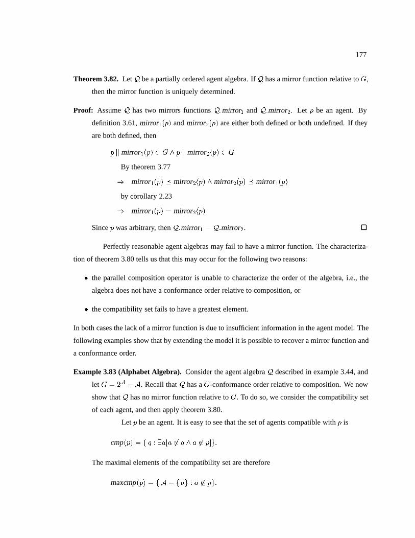
177

Theorem 3.82. LetQ be a partially ordered agent algebra. IfQ has a mirror function relative toG,

then the mirror function is uniquely determined.

Proof: AssumeQ has two mirrors functionsQ:mirror1 andQ:mirror2. Let p be an agent. By

definition 3.61,mirror1(p) andmirror2(p) are either both defined or both undefined. If they

are both defined, then

p kmirror1(p) 2 G ^ p kmirror2(p) 2 G

By theorem 3.77

) mirror1(p) � mirror2(p) ^mirror2(p) � mirror1(p)

by corollary 2.23

) mirror1(p) = mirror2(p)

Sincep was arbitrary, thenQ:mirror1 = Q:mirror2.

Perfectly reasonable agent algebras may fail to have a mirror function. The characteriza-

tion of theorem 3.80 tells us that this may occur for the following two reasons:

� the parallel composition operator is unable to characterize the order of the algebra, i.e., the

algebra does not have a conformance order relative to composition, or

� the compatibility set fails to have a greatest element.

In both cases the lack of a mirror function is due to insufficient information in the agent model. The

following examples show that by extending the model it is possible to recover a mirror function and

a conformance order.

Example 3.83 (Alphabet Algebra). Consider the agent algebraQ described in example 3.44, and

letG = 2A �A. Recall thatQ has aG-conformance order relative to composition. We now

show thatQ has no mirror function relative toG. To do so, we consider the compatibility set

of each agent, and then apply theorem 3.80.

Let p be an agent. It is easy to see that the set of agents compatible withp is

cmp(p) = f q : 9a[a 62 q ^ a 62 p]g:

The maximal elements of the compatibility set are therefore

maxcmp(p) = fA � f ag : a 62 pg:

178

Observe thatmaxcmp(p) is a set of incomparable agents. Thuscmp(p) does not have a

greatest element, and therefore, by theorem 3.80,Q does not have a mirror function relative

toG. BecauseG is the only set of agents that characterizes the order relative to composition,

Q has no mirror function relative to anyG.

Example 3.84 (Locked Alphabet Algebra). In this example we present an extension of exam-

ple 3.83 and we show that by adding extra information to the model it is possible to charac-

terize the order with a mirror function.

The locked alphabet algebraQ is defined as follows:

� Agents are of the formp = (A;L) whereA andL are disjoint subsets ofQ:A. The

alphabet ofp is �(p) = A [ L.

� rename(r)(p) is defined whenever�(p) � dom(r). In that caserename(r)(p) =

(r(A); r(L)), wherer is naturally extended to sets.

� proj(B)(p) = (A \B;L \B).

� p1 k p2 is defined wheneverL1 \ L2 = ;, A1 \ L2 = ; andA2 \ L1 = ;. In that case

p1 k p2 = (A1 [A2; L1 [ L2):

The additional set of signalsL is used by an agentp to indicate that no agentq can compose

with p if q uses signals inL.

Theorem 3.85. Let� be an order forQ such thatrename, proj andk are>-monotonic. Let

p = (A;L) andp0 = (A0; L0) be two agents. Thenp � p0 only if A � A0 [ L0 and

L � L0.

Proof: Consider the agentq = (A0;A� (A0 [L0)). Clearly,p0 k q is defined, sinceL0 \A�

(A0 [ L0) = ; andA0 \ L0 = ;. Therefore, sincek is >-monotonic andp � p0, also

p k q is defined. Hence:

L \A� (A0 [ L0) = ; ^ L \A0 = ; ^ A \A� (A0 [ L0) = ;

) L � A0 [ L0 ^ L \A0 = ; ^ A � A0 [ L0

) A � A0 [ L0 ^ L � L0:

The requirements ofrenameandproj are subsumed by those ofk.

179

We will consider the order such thatp � p0 if and only ifA � A0 [L0 andL � L0.

The proof that the operators are>-monotonic is left to the reader.

Note that the subset of agentsP = f (A;L) : L = ;g is closed under the operations

and thus constitutes a subalgebraP of Q. It is easy to show thatP is isomorphic to the

Alphabet Algebra of example 3.83. By extension, we consider the Locked Alphabet Algebra

a superalgebra of the Alphabet Algebra.

The order can be characterized as aG-conformance order relative to composition

whereG = D includes all the agents of the algebra. ClearlyG is downward closed relative

to�.

Let nowp0 = (A0; L0) be an agent, and consider the set of agentsq = (A;L) that

are compatible withp0. SinceG is the set of all agents, an agentq is compatible withp0 if and

only if q k p0 is defined, that is

L \ L0 = ; ^ A \ L0 = ; ^ A0 \ L = ;

which translates to

cmp(p0) = f (A;L) : A \ L = ; ^A � A� L0 ^ L � A� (A0 [ L0)g:

Note that ifA � A � L0 andL � A � (A0 [ L0), thenA � A0 [ (A � (A0 [ L0)) and

L � A � (A0 [ L0). Therefore, the agentq = (A0;A� (A0 [ L0) is the greatest element of

cmp(p0).

Theorem 3.86. Let p = (A;L) andp0 = (A0; L0) be two agents. Thenp � p0 if and only if

p k (A0;A� (A0 [ L0)) is defined.

Thereforemirror(p0) = (A0;A� (A0 [ L0)) is a mirror function relative toG, and

Q has aG-conformance order relative to composition.

Example 3.87 (IO Agent Algebra). Consider the IO agent algebraQ described in example 3.48

and letG be the set of agents that have no inputs. ThenQ has aG-conformance order relative

to composition. We now show thatQ has no mirror function relative toG. Let p0 = (I 0; O0)

be an agent. The set of agents compatible withp0 is

cmp(p0) = f q = (Iq; Oq) : Iq � O0 ^ I 0 � Oq � A�O0g:

The maximal elements of the compatibility set are therefore

maxcmp(p0) = f q = (Iq; Oq) : Iq = O0 ^ I 0 � Oq � A�O0g:

180

Since the agents inmaxcmp(p0) are incomparable,cmp(p0) does not have a greatest element,

and therefore, by theorem 3.80,Q does not have a mirror function relative toG.

Notice how every maximal element imposes a particular constraint for an agent to

refine another. Letp = (I;O) andp0 = (I 0; O0) be two agents. Then the maximal element

q1 = (O0; I 0) characterizes an order (which is not>-monotonic) such that

p � p0 , I � I 0 ^O � O0 ^O \ I 0 = ;:

On the other hand, the maximal elementq2 = (O0;A� O0) characterizes the different order

(again not>-monotonic) such that

p � p0 , I � A�O0 ^O � O0 ^O � O0:

In other words,q1 provides the constraint on the inputs, whileq2 constrains the outputs. Note

that in this case these two maximal elements are sufficient to characterize the order, which is

equal to the intersection of the two orders described.

Example 3.88 (Locked IO Agent Algebra). In this example we present an extension of exam-

ple 3.87 and we show that by adding extra information to the model it is possible to charac-

terize the order with a mirror function.

The locked IO Agent algebraQ is defined as follows:

� Agents are of the formp = (I;O; L) whereI, O andL are disjoint subsets ofQ:A.

The alphabet ofp is �(p) = I [O [ L.

� rename(r)(p) is defined whenever�(p) � dom(r). In that caserename(r)(p) =

(r(I); r(O); r(L)), wherer is naturally extended to sets.

� proj(B)(p) is defined wheneverI � B. In that case,proj(B)(p) = (I;O\B;L\B).

� p1 k p2 is defined whenever(O1 [L1)\ (O2 [L2) = ;, I1 \L2 = ; andI2 \L1 = ;.

In that case

p1 k p2 = ((I1 [ I2)� (O1 [O2); O1 [O2; L1 [ L2):

The additional set of signalsL is used by an agentp to indicate that no agentq can compose

with p if q uses signals inL.

181

Theorem 3.89. Let� be an order forQ such thatrename, proj andk are>-monotonic. Then

p � p0 only if I � I0,O0 � O � O0 [ L0 andL � L0.

Proof: The proof is similar to the proof of theorem 2.30. Letp = (I;O; L) and p0 =

(I 0; O0; L0) be two agents such thatp � p0. Then consider the agentq = (O0; I 0;A �

(I 0[O0[L0)) and deduce the conditions for whichrename(r)(p), proj(B)(p) andpkq

are all defined.

We will consider the order such thatp � p0 exactly whenI � I0,O0 � O � O0[L0

andL � L0.

Theorem 3.90. The functionsrename, proj andk are>-monotonic with respect to�.

Proof: The proof is similar to the proof of theorem 2.31.

Note that the subset of agentsP = f (I;O; L) : L = ;g is closed under the opera-

tions and thus constitutes a subalgebraP of Q. It is easy to show thatP is isomorphic to the

IO Agent Algebra of example 3.87. By extension, we consider the Locked IO Agent Algebra

a superalgebra of the IO Agent Algebra.

The order can be characterized as aG-conformance order relative to composition,

whereG = f (;; O; L)g includes all the only the agents with no inputs. ClearlyG is down-

ward closed relative to�.

Let nowp0 = (I 0; O0; L0) be an agent, and consider the set of agentsq = (I;O; L)

compatible withp0. We have

q k p0 = ((I [ I 0)� (O [O0); O [O0; L [ L0);

with the following conditions for membership inG and for definedness:

I [ I � O [O0;

(O [ L) \ (O0 [ L0) = ;;

I \ L0 = ; ^ L \ I 0 = ; ^ L \ L0 = ;:

These conditions imply (since also for each agent,I,O andL must be disjoint) that

; � I � O0

I 0 � O � A� (O0 [ L0)

; � L � A� (O [O0 [ L0)

182

Notice that the two agentsq1 = (I;O [ f ag; L), andq2 = (I;O; L [ f ag) are comparable

andq1 � q2. Therefore the set of compatible agents ofp0 has a greatest element. It is easy to

show that the greatest element is also a mirror function, so that

mirror(p0) = (O0; I 0;A� (I 0 [O0 [ L0)):

Hence, the algebra also has aG-conformance order relative to composition.

In the particular case of the simple IO agents,p0 is of the formp0 = (I 0; O0; ;).

Hencemirror(p0) = (O0; I 0;A � (I 0 [ O0)). Note how all the maximal elements found in

example 3.87 are contained inmirror(p0) in the superalgebra. In the superalgebra, however,

the compatibility set is extended upwards by agents that converge to a unique greatest element.

Example 3.91 (Dill’s IO Agent Algebra). We have seen in example 3.54 that the Dill’s IO Agent

Algebra does not have a characterization in terms of conformance relative to composition. It

is therefore impossible to find a mirror function in this case. We will however reconsider this

example when we restrict the order to agents that share the same alphabet, below.

In this section we have seen examples of agent algebras that don’t have a mirror function,

despite having aG-conformance order relative to composition (see example 3.83 and example 3.87).

The solution adopted in those cases consists of augmenting the model with enough information to

let a single environment characterize the order. In the next two sections we explore alternative

solutions that consist of adding some extra condition to the definition of the mirror function in order

to restrict the size of the compatibility set.

3.3.1 Mirrors with Predicates

Let Q be an ordered agent algebra, and letp0 be an agent. IfQ has aG-conformance

order relative to composition, then the compatibility setcmp(p0) of p0 completely characterizes the

set of agentsp such thatp � p0 (see lemma 3.75). Each individual agentq in the compatibility set

contributes to the characterization of the order by discriminating among two sets: the set of agents

p that are compatible withq do not conform to p0; and the set of agentsp that are compatible with

q thatpotentially conform top0. In other words, each compatible agent has a particular view of the

conformance order.

When a mirror function exists, one agent (the greatest element) has an exact view of the

conformance order. In that case, the compatibility set ofp0 is equal to the set of agents that conform

to mirror(p0), and, vice-versa, the compatibility set ofmirror(p0) is equal to the set of agents that

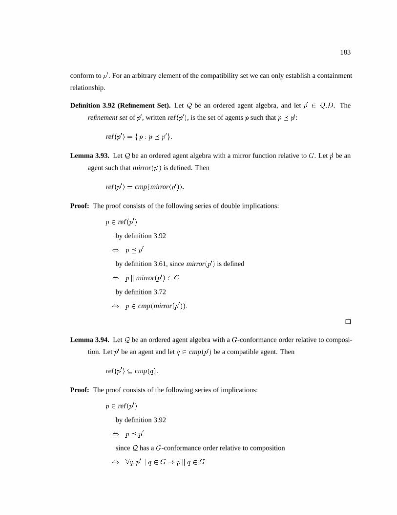
183

conform top0. For an arbitrary element of the compatibility set we can only establish a containment

relationship.

Definition 3.92 (Refinement Set). Let Q be an ordered agent algebra, and letp0 2 Q:D. The

refinement set of p0, written ref(p0), is the set of agentsp such thatp � p0:

ref(p0) = f p : p � p0g:

Lemma 3.93. LetQ be an ordered agent algebra with a mirror function relative toG. Let p0 be an

agent such thatmirror(p0) is defined. Then

ref(p0) = cmp(mirror(p0)):

Proof: The proof consists of the following series of double implications:

p 2 ref(p0)

by definition 3.92

, p � p0

by definition 3.61, sincemirror(p0) is defined

, p kmirror(p0) 2 G

by definition 3.72

, p 2 cmp(mirror(p0)):

Lemma 3.94. LetQ be an ordered agent algebra with aG-conformance order relative to composi-

tion. Letp0 be an agent and letq 2 cmp(p0) be a compatible agent. Then

ref(p0) � cmp(q):

Proof: The proof consists of the following series of implications:

p 2 ref(p0)

by definition 3.92

, p � p0

sinceQ has aG-conformance order relative to composition

, 8q; p0 k q 2 G) p k q 2 G

184

sinceq 2 cmp(p0), q k p0 2 G, therefore

) p k q 2 G

by definition 3.72

, p 2 cmp(q):

These two results are represented graphically in figure 3.1 and figure 3.2. Given an agentq

������������������������������������

������������������������������������

�������������������������������������������������������������������������������������������������������������������������������������������������������������������������������������������������������������������������������������������������������������������������������������������������������������������������������������������������������������������������������������������������������������������

�������������������������������������������������������������������������������������������������������������������������������������������������������������������������������������������������������������������������������������������������������������������������������������������������������������������������������������������������������������������������������������������������������������������

p0mirror(p0)

cmp(p0)

ref(p0)

q

mirror(q)

cmp(q)

Figure 3.1: Refinement sets and compatibility sets with mirrors

in the compatibility set ofp0, we call thediscrimination set of q the set of agents thatq discriminates

exactly for the purpose of conformance top0.

Definition 3.95 (Discrimination Set). Let Q be an ordered agent algebra with aG-conformance

order relative to composition. Letp0 be an agent and letq 2 cmp(p0) be a compatible agent.

Thediscrimination set of q overp0 is the set

disp0(q) = f p : p � p0 , p k q 2 Gg:

Lemma 3.96 (Discrimination). Let Q be an ordered agent algebra with aG-conformance order

relative to composition. Letp0 be an agent and letq 2 cmp(p0) be a compatible agent. Then

disp0(q) = (Q:D � cmp(q)) [ ref(p0):

Proof: We must show thatp 2 (Q:D � cmp(q)) [ ref(p0) if and only if p � p0 , p k q 2 G. For

the forward direction we consider the following two cases:

185

����������������������������������������������������������������������������������������������������������������������������������������������������������������������������������������������������������������������������������������������������������������������������������������������������������������������������������������������������������������������������������������������������������������������������������������������������������������������������������������������������������������������������������������������������������������������������������������������������������������������������������������������������������������������������������������������������������������������������������������������������������������������������������������

����������������������������������������������������������������������������������������������������������������������������������������������������������������������������������������������������������������������������������������������������������������������������������������������������������������������������������������������������������������������������������������������������������������������������������������������������������������������������������������������������������������������������������������������������������������������������������������������������������������������������������������������������������������������������������������������������������������������������������������������������������������������������������������

������������������������������������������������������������������������������������������������������������������������������������������������������������������������������������������������������������������������������������������

������������������������������������������������������������������������������������������������������������������������������������������������������������������������������������������������������������������������������������������

������������������������������������������������������������������������������������������������������������������������������������������������������������������������������������������������������������������

������������������������������������������������������������������������������������������������������������������������������������������������������������������������������������������������������������������

p0

cmp(p0)

ref(p0)

q1

cmp(q1)

q2

cmp(q2)

q3

cmp(q3)

Figure 3.2: Compatibility sets of compatible agents

� If p 2 Q:D � cmp(q), thenp 62 cmp(q) andp k q 62 G. By lemma 3.94,ref(p0) �

cmp(q), thereforep 62 ref(p0). Thereforep 6� p0. Hencep � p0 , p k q 2 G.

� If p 2 ref(p0), thenp � p0. By lemma 3.94,ref(p0) � cmp(q), thereforep 2 cmp(q).

Thereforep k q 2 G. Hencep � p0 , p k q 2 G.

For the reverse direction, letp be an agent such thatp � p0 , p k q 2 G. We then consider

the following two cases:

� If p � p0, thenp 2 ref(p0) and thereforep 2 (Q:D � cmp(q)) [ ref(p0).

� If p 6� p0, then, by hypothesis,p k q 62 G. Hencep 62 cmp(q). Thereforep 2

Q:D � cmp(q), and consequentlyp 2 (Q:D � cmp(q)) [ ref(p0).

Corollary 3.97. LetQ be an ordered agent algebra with a mirror function relative toG. Let p0 be

an agent such thatmirror(p0) is defined. Then

disp0(mirror(p0)) = Q:D:

186

Proof: The proof consists of the following equalities:

disp0(mirror(p0)) = f p : p � p0 , p kmirror(p0) 2 Gg

by lemma 3.96

= (Q:D � cmp(mirror(p0))) [ ref(p0)

by lemma 3.93

= (Q:D � ref(p0)) [ ref(p0)

= Q:D:

The above results show that every compatible agent can be used as a “mirror” if the

characterization is restricted to its discrimination set. This suggests an extended notion of mirror

function, whose applicability is subject to the satisfaction of a predicate.

Definition 3.98 (Mirror Function with Predicate). LetQ be an ordered agent algebra and letG be

a downward closed set of agents ofQ. For each agentp0, let pred(p0) � Q:D be a predicate

overQ:D such thatref(p0) � pred(p0). Then,Q has a mirror function with predicate relative

to G if and only if

1. Q:mirror (which we may simply write as “mirror” when there is no ambiguity about

what agent algebra is being considered) is a partial function fromD toD,

2. mirror(p) is defined if and only if there existsq such thatp k q 2 G,

3. If p 2 pred(p0), then p � p0 if and only if either mirror(p0) is undefined orp k

mirror(p0) 2 G.

Corollary 3.99. LetQ be an ordered agent algebra with a mirror function with predicate relative to

G. Then, for all agentsp andp0, the following two statements are equivalent

1. p � p0

2. p 2 pred(p0) and eithermirror(p0) is undefined orp kmirror(p0) 2 G.

The regular mirror function can be interpreted as a mirror function with predicate by

simply setting for all agentsp0

pred(p0) = Q:D:

187

Hence mirror functions with predicate are more general than the regular mirror functions.

Unfortunately mirror functions with predicate do not enjoy the same characterization in

terms ofG-conformance relative to composition and greatest elements of the compatibility set (see

theorem 3.80). A simple counterexample is obtained by considering the predicate

pred(p0) = f p : p � p0g:

In this case, any agent of the compatibility set can function as the mirror. This extreme case is,

of course, useless, since the complexity of checking membership with the predicate is the same as

the complexity of checking conformance. Mirror functions with predicate are therefore most useful

when the predicate is relatively easy to check.

The choice of the predicate is guided by the following result.

Theorem 3.100. Let Q be an ordered agent algebra with aG-conformance order relative to com-

position. For all agentsp0, let mirror(p0) 2 cmp(p0) be a compatible agent (mirror(p0) is

undefined ifcmp(p0) = ;), and letpred(p0) � Q:D be a predicate. Then the following two

conditions are equivalent:

1. mirror is a mirror function with predicatepred relative toG.

2. For all agentsp0, ref(p0) � pred(p0) and if mirror(p0) is defined, thenpred(p0) �

disp0(mirror(p0)).

Proof: For the forward direction, by definition 3.98, for all agentsp0, ref(p0) � pred(p0). Let now

p0 be an agent such thatmirror(p0) is defined and letp 2 pred(p0) be an agent. Then,

p 2 pred(p0)

by definition 3.98, sinceQ has a mirror function with predicate relative toG

) p � p0 , p kmirror(p0) 2 G

by definition 3.95

) p 2 disp0(mirror(p0)):

Hence,pred(p0) � disp0(mirror(p0)).

For the reverse direction, assumeref(p0) � pred(p0) � disp0(mirror(p0)). Clearly

mirror is a partial function, andmirror(p) is defined if and only if there existsq such that

p k q 2 G. Let nowp be an agent such thatp 2 pred(p0). We must show thatp � p0 if and

only if eithermirror(p0) is undefined orp kmirror(p0) 2 G. We consider two cases.

188

Assumemirror(p0) is undefined. Then, by hypothesis,cmp(p0) = ;, and there-

fore, sinceQ has aG-conformance order relative to composition, for all agentsp, p � p0.

Therefore,p � p0 if and only if mirror(p0) is undefined.

Conversely, assumemirror(p0) is defined. Then,

p 2 pred(p0)

since by hypothesispred(p0) � disp0(mirror(p0))

) p 2 disp0(mirror(p0))

by definition 3.95

) p � p, p kmirror(p0) 2 G:

Hencemirror is a mirror function with predicatepred relative toG.

The greater the element in the compatibility set, the larger the discrimination set.

Lemma 3.101. LetQ be an ordered agent algebra with aG-conformance order relative to compo-

sition. Letp0 be an agent and letq1 andq2 be compatible agents such thatq1 � q2. Then

disp0(q1) � disp0(q2):

Since greater elements have larger discrimination sets, and sincepred(p0) must be a subset

of the discrimination set ofmirror(p0), it is convenient to choose a maximal element of the compat-

ibility set for mirror(p0). In this way, we have the maximum flexibility in choosing a predicate that

is computationally easy to check. However, unlike regular mirror functions, the mirror of an agent

with predicate is not necessarily a maximal element of the compatibility set.

The following examples show the use of mirror functions with predicate in the cases

where a regular mirror function does not exist.

Example 3.102 (IO Agent Algebra). Example 3.87 shows that the IO agent algebra does not have

a mirror function relative toG, despite having aG-conformance order relative to composition.

In this example we show how to derive a mirror function with predicate.

Let p0 = (I 0; O0) be an agent. As shown in example 3.87, the agentq1 = (O0; I 0)

is a maximal element of the compatibility set ofp0. We now wish to useq1 as a mirror ofp0

189

with the use of a predicate. To do so, we compute the discrimination set ofq1:

disp0(q1) = (Q:D � cmp(q1)) [ ref(p0)

= (Q:D � f (I;O) : I � I 0 ^O0 � O � A� I 0g) [ f (I;O) : I � I 0 ^O = O0g

= f (I;O) : I 0 � I _O � O0 _A� I 0 � Og [ f (I;O) : I � I 0 ^O = O0g

= f (I;O) : I 0 � I _O � O0 _A� I 0 � O _ (I � I 0 ^O = O0)g

Recall thatpred(p0) must includeref(p0). A reasonable choice forpred(p0) in this case is the

following:

pred(p0) = f p : �(p) � �(p0)g:

This predicate is easy to check for finite alphabets, and satisfies the conditionref(p0) �

pred(p0) � disp0(q1). Therefore, by theorem 3.100,Q has a mirror function with predicate

relative toG, where

mirror((I;O)) = (O; I); pred(p0) = f p : �(p) � �(p0)g:

Note thatq1 is not the only compatible agent that can be used as a mirror with the above

predicate. For example, the maximally compatible agentq2 = (O0;A�O0) has the following

discrimination set:

disp0(q2) = (Q:D � cmp(q2)) [ ref(p0)

= (Q:D � f (I;O) : I � A�O0 ^O = O0g) [ f (I;O) : I � I 0 ^O = O0g

= f (I;O) : A�O0 � I _O 6= O0g [ f (I;O) : I � I 0 ^O = O0g

= f (I;O) : A�O0 � I _O 6= O0 _ (I � I 0 ^O = O0)g

It is easy to check that the conditionref(p0) � pred(p0) � disp0(q2) is satisfied. Hence,Q

has also the following mirror function with predicate:

mirror((I;O)) = (O;A�O); pred(p0) = f p : �(p) � �(p0)g:

We have noted how mirror functions with predicate lose the characterization in terms of

conformance order that simple mirror functions have. For a restricted case, however, we can re-

duce a mirror function with predicate to a regular mirror function by extending the model as in

example 3.84 and example 3.88. The construction consists of augmenting the model by providing

each agent with the information conveyed by the predicate of their mirror. This construction is

190

still somewhat preliminary, as it doesn’t guarantee a downward closed conformance set. In addi-

tion, the conformance set does not necessarily enjoy the properties that are necessary for applying

theorem 3.119 below.

Theorem 3.103. LetQ be an agent algebra with a mirror function with predicate relative toG, such

that pred(p) = pred(mirror(p)). If G is downward closed, then the agent algebraQ has a

mirror function relative toG, where

� Q:D = f (p; set) : p 2 Q:D ^ set � Q:D ^ pred(p) \ set = ;g

� (p; set) � (p0; set0) if and only if eitherQ:mirror(p0) is not defined, or, if defined,

set � set0;

pred(p) � set0 [ pred(p0) and

p k Q:mirror(p0) 2 G:

� proj(B)((p; setp)) = (proj(B)(p);proj(B)(setp)) if all quantities are defined.

� rename(r)((p; setp)) = (rename(r)(p); rename(r)(setp)) if all quantities are defined.

� (p; setp) k (q; setq) is defined if and only if

p k q is defined;

pred(p) \ setq = ;;

pred(q) \ setp = ; and

setp \ setq = ;:

In that case

(p; setp) k (q; setq) = (p k q; setp [ setq)

� Q:mirror((p; set)) is defined if and only ifQ:mirror(p) is defined. In that case,

Q:mirror((p; set)) = (Q:mirror(p);Q:D � (set [ pred(p))):

� G = G� 2Q:D

Proof: We must show thatQ:mirror is a mirror function relative toG.

ClearlyQ:mirror is a partial function fromQ:D to Q:D. Also, if, for an agent

(p; set), Q:mirror((p; set)) is defined, thenQ:mirror((p; set)) k (p; set) 2 G. Conversely,

191

if (q; setq) k (p; set) 2 G, thenq k p 2 G, henceQ:mirror(p) is defined, and therefore

Q:mirror((p; set)) is defined.

Assume now that(p; set) � (p0; set0), and assume thatQ:mirror((p0; set0)) =

(Q:mirror(p0);Q:D � (set0 [ pred(p0))) is defined. Then

� By hypothesisp k Q:mirror(p0) 2 G.

� pred(p) \ (Q:D � (set0 [ pred(p0))) = ;, sincepred(p) � set0 [ pred(p0).

� pred(Q:mirror(p0)) \ set = ;, since by hypothesispred(Q:mirror(p0)) = pred(p0),

pred(p0) \ set0 = ; andset � set0.

� set \ (Q:D � (set0 [ pred(p0))) = ;, sinceset � set0.

Therefore(p; set) k (Q:mirror(p0);Q:D � (set0 [ pred(p0))) 2 G.

Conversely, assume(p; set) k (Q:mirror(p0);Q:D � (set0 [ pred(p0))) 2 G. Then

� set � set0 [ pred(p0), sinceset \ (Q:D � (set0 [ pred(p0))) = ;. In addition,

set \ pred(p0) = ;, sinceset \ pred(Q:mirror(p0)) = ; andpred(Q:mirror(p0)) =

pred(p0). Therefore,set � set0.

� pred(p) � set0 [ pred(p0), sincepred(p) \ (Q:D � (set0 [ pred(p0))) = ;.

� By hypothesisp k Q:mirror(p0) 2 G.

Therefore(p; set) � (p0; set0).

Similarly, if Q:mirror((p0; set0)) is not defined, then(p; set) � (p0; set0) if and

only if Q:mirror((p0; set0)) is not defined.

Therefore, by definition 3.61,Q:mirror is a mirror function forQ relative toG.

Theorem 3.104. LetQ andQ be as in theorem 3.103. Then the functione :Q:D 7! Q:D such that

for all agentsp

e(p) = (p; ;)

is an embedding.

Proof: It is easy to show thate commutes with the operators of the algebra, that is, for example,

that

proj(B)(e(p)) = e(proj(B)(p)):

192

To complete the proof we must show thatp � p0 if and only if (p; ;) � (p0; ;).

Let p andp0 be such thatp � p0. If Q:mirror(p0) is not defined, then(p; ;) �

(p0; ;). Alternatively, assumeQ:mirror(p0) is defined. Then, sincep � p0, p 2 pred(p0) and

pkQ:mirror(p0) 2 G. Sincepred is monotonic relative to�, pred(p) � pred(p0). Therefore,

by definition ofQ, (p; ;) � (p0; ;).

Conversely, assume(p; ;) � (p0; ;). If Q:mirror(p0) is not defined thenp � p0.

Alternatively, assumeQ:mirror(p0) is defined. Then, by definition ofQ, pred(p) � pred(p0),

and therefore, sincep 2 pred(p), p 2 pred(p0). In addition,pkQ:mirror(p0) 2 G. Therefore,

by definition 3.98, alsop � p0.

Hence,p � p0 if and only if (p; ;) � (p0; ;).

Corollary 3.105. Let Q andQ be as in theorem 3.103 such thatG is downward closed, and let

(p0; ;) be an agent ofQ. If (p; set) � (p0; ;), thenset = ;.

The above results show that ifp0 is an agent inQ, then the mirror of(p0; ;) in Q charac-

terizes exactly the agentsp such thatp � p0.

3.3.2 Mirrors and Subalgebras

In the previous section we have employed a predicate to focus the application of the mirror

function to only those agents that the mirror can discriminate. Here we use an alternative approach,

and consider only a subset of the agents to reduce the size of the compatibility sets. We choose

the subset so that it is downward closed, and closed under parallel composition, thus effectively

constructing a subalgebra when the operators of projection and renaming are removed from the

signature. Since the compatibility sets are smaller, subalgebras have a greater chance to have a

G-conformance order relative to composition and a mirror function.

An example that is particularly useful in practice is the subset of agents that have the same

alphabet. In particular, we are interested in studying the conformance order and the corresponding

mirror function for algebras whose order satisfies the constraint

p � p0 ) �(p) = �(p0):

Note that if�(p) = �(q), then�(pkq) = �(p) = �(q). Therefore the subset of agents with a certain

alphabet that satisfy the above constraint is closed under parallel composition and thus constitute

a subalgebra of the original agent algebra (restricted to parallel composition only). Note also that

193

the projection and renaming operators have no effect in determining conformance relative to com-

position and mirror functions. Therefore, the results of the previous sections apply to this restricted

case, provided that the necessary restrictions on the alphabet are enforced throughout. Projection

and renaming can be used, instead, to transition from one subalgebra to another subalgebra with

a different alphabet. This will be useful in solving the local specification synthesis problem under

these specific assumptions.

Let Q be an agent algebra and assume that for all alphabetsA, the algebraP such that

P:D = f p : �(p) = Ag is a subalgebra ofQ and is closed under�. Assume also that each subal-

gebra has aG-conformance order relative to composition and a mirror function relative toG. Note

that sinceP:D must be downward closed for all alphabets,p � p0 only if �(p) = �(p0). The

results obtained in the subalgebras can be rephrased in terms of the original algebra by restricting

the definitions of conformance order and mirror function to apply only when the alphabets of the

agents involved are the same. Note that we arenot changing the definition of conformance, but we

are simply reflecting the restrictions of the subalgebra in the superalgebra.

Definition 3.106. LetQ be an agent algebra and letG be a downward closed set of agents ofQ. Q

has asame alphabet G-conformance order relative to composition if and only if for all agents

p andp0, p � p0 if and only if �(p) = �(p0) and for all agentsq such that�(q) = �(p0), if

p0 k q 2 G thenp k q 2 G.

Definition 3.107. LetQ be an ordered agent algebra and letG be a downward closed set of agents

of Q. Then,Q has a same alphabet mirror function relative to G if and only if

1. Q:mirror is a partial function fromD toD,

2. mirror(p) is defined if and only if there existsq such that�(q) = �(p) andp k q 2 G,

3. p � p0 if and only if�(p) = �(p0) and eithermirror(p0) is undefined orpkmirror(p0) 2

G.

The additional conditions in these definitions consistently restrict the alphabets of the

agents involved to the alphabet of the agent for which we are considering the mirror.

In particular we are interested in the characterization of the mirror in terms of the greatest

element of the compatibility set and of conformance relative to composition.

Definition 3.108 (Compatibility Set). LetQ be an ordered agent algebra andG a downward closed

set of agents. Thealphabet invariant G-compatibility set of an agentp, written cmp(p), is

194

defined as follows:

cmp(p) = f q : �(q) = �(p) ^ p k q 2 Gg

Theorem 3.109. LetQ be an ordered agent algebra and letG be a downward closed set of agents.

Then the following two statement are equivalent:

1. Q has an alphabet invariant mirror function relative toG.

2. Q has an alphabet invariantG-conformance order relative to composition, and for all

agentsp0, cmp(p0) is either empty or if it is not empty it has a greatest element.

These definitions and results apply, for example, to Dill’s trace structure algebra [34]

and can be applied to any model in which substitutability in defined only for agents that share the

same interface. These notion can however be generalized to any arbitrary equivalence relation that

partitions the sets of agents into equivalence classes that are closed under composition and under

the agent ordering. We omit the details of this generalization.

3.3.3 Construction of Algebras

In this section we explore conformance and mirrors for the direct product of algebras and

for subalgebras. We begin by showing that if two agent algebras have a conformance order, then

the agent order in their product is weaker than the corresponding conformance order. We also show

that the product does have a conformance order, in case the algebras have a mirror function, and the

mirror is defined for all agents.

Theorem 3.110. Let Q1 andQ2 be agent algebras with aG1 andG2-conformance order, respec-

tively. Let Q = Q1 � Q2 be the direct product (definition 2.13) ofQ1 andQ2 and let

G = G1 � G2. Then for allp; p0 2 Q:D, if p �Q p0 then for all expression contextsE, if

E[p0] 2 G thenE[p] 2 G.

Proof: Let p = hp1; p2i andp0 = hp01; p02i be agents such thatp � p0. The proof consists of the

195

following series of implications:

p � p0

by definition 2.13

, p1 �Q1p01 ^ p2 �Q2

p02

by hypothesis

, (8E;E[p01] 2 G1 ) E[p1] 2 G1) ^ (8E;E[p02] 2 G2 ) E[p2] 2 G2)

by definition 2.13

) 8E;E[p0] 2 G) E[p] 2 G:

Unfortunately the reverse of the last implication in the proof above does not hold, that is

Q does not necessarily have aG-conformance order. This is because a contextE may be defined

for an agentp1, while it may not be defined for the pairhp1; p2i. However, the result holds in the

presence of mirror functions, when the mirror function is always defined. In that case, in fact, the

expression contexts can be reduced to a single environment, and the difficulty above disappears.

Theorem 3.111. Let Q1 andQ2 be agent algebras with a mirror function relative toG1 andG2,

respectively, such that for all agentsp, mirror(p) is defined. LetQ = Q1 � Q2 be the

direct product (definition 2.13) ofQ1 andQ2 and letG = G1 � G2. Then for all agents

(p1; p2) 2 Q:D, mirror((p1; p2)) = (mirror(p1);mirror(p2)) is a mirror function forQ

relative toG.

Proof: ClearlyQ:mirror is a partial (in fact, total) function. Sincemirror is always defined, we

must show that for allp = hp1; p2i there existsq such thatp k q 2 G.

mirror(hp1; p2i)#

by hypothesis

, mirror(p1)# ^mirror(p2)#

by definition 3.61

, (9q1; p1 k q1 2 G1) ^ (9q2; p2 k q2 2 G2)

by definition 2.13

, 9hq1; q2i; hp1; p2i k hq1; q2i 2 G

, 9q; p k q 2 G

196

It remains to show that for allp; p0 2 Q:D, p � p0 if and only if p k mirror(p0) 2 G. Let

p = hp1; p2i andp0 = hp01; p02i.

p � p0

, hp1; p2i � hp01; p02i

by definition 2.13

, p1 � p01 ^ p2 � p02

by definition 3.61, sincemirror(p01) andmirror(p02) are both defined

, p1 kmirror(p01) 2 G1 ^ p2 kmirror(p02) 2 G2

by definition 2.13

, hp1; p2i k hmirror(p01);mirror(p02)i 2 G

by hypothesis

, hp1; p2i kmirror(hp01; p02)i 2 G

, p kmirror(p0) 2 G

In the rest of the section we consider subalgebras. We distinguish between two cases.

For the first case, we consider subalgebras that preserve the agent ordering, as described in defini-

tion 2.41. We show that, in that case, the conformance order in the subalgebra becomes stronger,

since fewer contexts may contribute to the notion of conformance. Consequently, the subalgebra

may fail to have a conformance order. If however the superalgebra has a mirror function, and if the

subalgebra is closed under that mirror function, then the subalgebra has the same mirror function

and therefore a conformance order.

Theorem 3.112. Let Q0 be an ordered agent algebra with aG0-conformance order and letQ be a

subalgebra ofQ0. LetG = G0 \Q:D. Then for all agentsp andp0 in Q, if p �Q p0 then for

all expression contextsE overQ, if E[p0] 2 G, thenE[p] 2 G.

Proof: Let E 0 be the set of expressions overQ0, and letE be the set of expressions overQ. Note

that sinceQ is a subalgebra ofQ0, an expression overQ is also an expression overQ0, and

thereforeE � E0.

Let nowp andp0 be elements ofQ:D. The proof consists of the following series of

197

implications.

p �Q p0

by definition 2.41

, p �Q0 p0

sinceQ0 has aG0-conformance order, by definition 3.26

, 8E 2 E 0; E[p0] 2 G0 ) E[p] 2 G0

sinceQ:D is closed inQ0:D under the operators,G = G0 \Q:D, E � E 0,

and since for allp 2 Q:D, E[p0] 2 G0 , E[p0] 2 G,

) 8E 2 E ; E[p0] 2 G) E[p] 2 G

The reverse of the last implication does not hold. In fact, while it is true that ifE[p] 2 G,

thenE[p] 2 G0, the subalgebra can only consider a subset of the contexts, and may therefore be

unable to completely characterize the order.

Theorem 3.113. Let Q0 be an ordered agent algebra with a mirror functionmirror relative toG0

and letQ be a subalgebra ofQ0 closed undermirror. Let G = G0 \ Q:D. ThenQ has a

mirror function relative toG.

Proof: We show that thatmirror is a mirror function forQ relative toG. Clearlymirror is a partial

function.

Let now p 2 Q:D be an agent. Ifmirror(p) is defined, then, sinceQ is closed

under mirror,mirror(p) 2 Q:D. Sincemirror is a mirror function relative toG0 for Q0,

by lemma 3.62,p k mirror(p) 2 G0. Sincep 2 Q:D, mirror(p) 2 Q:D, and sinceQ is

closed under parallel composition,p k mirror(p) 2 Q:D. Therefore, sinceG = G0 \ Q:D,

p k mirror(p) 2 G. Hence, ifmirror(p) is defined, then there existsq (i.e., mirror(p)) such

thatp k q 2 G.

Conversely, if there existsq 2 Q:D such thatp k q 2 G, then, sinceQ � Q0, also

p k q 2 G0. Therefore, by definition 3.61,mirror(p) is defined.

Let nowp 2 Q:D andp0 2 Q:D. It remains to show thatp � p0 if and only if

198

eithermirror(p0) is undefined orp kmirror(p0) 2 G.

p �Q p0

sinceQ � Q0

, p �Q0 p0

sinceQ0 has a mirror function relative toG0, by definition 3.61

, mirror(p0)" _ p kmirror(p0) 2 G0

sinceQ is closed under mirror andG = G0 \Q:D

, mirror(p0)" _ p kmirror(p0) 2 G

For the second case, we consider a subalgebra that does not preserve the order, but that

is simply closed under the operators. This notion of subalgebra corresponds to the one described

in definition 2.18. We assume that both the superalgebra and the subalgebra have a conformance

order. We show that the order in the subalgebra is stronger than the order in the superalgebra, since

in the subalgebra case there are fewer context to be satisfied in the definition of conformance.

Theorem 3.114. Let Q0 be an ordered agent algebra with aG0-conformance order and letQ be a

subalgebra ofQ0. LetG = G0 \ Q:D and assumeQ has aG-conformance order. Then for

all agentsp andp0 in Q,

p �Q0 p0 ) p �Q p0:

Proof: Let p andp0 be elements ofQ:D. The proof consists of the following series of implications.

p �Q0 p0

sinceQ0 has aG0-conformance order, by definition 3.26

, 8E 2 E 0; E[p0] 2 G0 ) E[p] 2 G0

sinceQ:D is closed inQ0:D under the operators,G = G0 \Q:D, E � E 0,

and since for allp 2 Q:D, E[p0] 2 G0 , E[p0] 2 G,

) 8E 2 E ; E[p0] 2 G) E[p] 2 G

sinceQ has aG-conformance order, by definition 3.26

, p �Q p0

199

3.4 Local Specification Synthesis

With conformance we have addressed the problem of characterizing substitutability under

all possible contexts. Relative conformance has been introduced to reduce (whenever possible)the

complexity of the problem by considering only a limited set of contexts. Relative conformance,

however, when applicable, does not change the notion of substitutability, since, in that case, relative

and general conformance coincide (see theorem 3.42).

In this section we address the problem of deriving the local specification for an agent in

a context, such that when an agent that satisfies the local specification is substituted in the context,

the resulting system satisfies a global specification. Instances of this problem include supervisory-

control synthesis [4], the rectification and optimization problem [13], and protocol conversion [73].

We will show that, under certain conditions, a mirror function provides us with a closed form solu-

tion.

Definition 3.115 (Local Specification). LetQ be an ordered agent algebra,E an expression con-

text, and letp0 be an agent. Alocal specification for p0 in E is an agentq such that for all

agentsp,

p � q , E[p] � p0:

In the rest of this section we address the problem of deriving the local specificationq,

given the expression contextE and the global specificationp0. The solution involves the use of the

mirror function. However, to solve the equation for the local specification, the conformance set must

have some additional closure properties. We call a conformance set with these additional properties

a rectification set.

Definition 3.116 (Rectification Set). LetQ be an agent algebra. A setG � Q:D is arectification

set if it satisfies the following requirements:

Downward closure If p0 2 G andp � p0, thenp 2 G.

Closure under projection If p 2 G, then for all alphabetsB, proj(B)(p) is defined and

proj(B)(p) 2 G.

Closure under inverse projection If p 2 G, then for all alphabetsB and all agentsp0, if

proj(B)(p0) = p thenp0 2 G.

200

Closure under renaming If p 2 G, then for all bijectionsr, if rename(r)(p) is defined then

rename(r)(p) 2 G.

An agent algebra must be normalizable to synthesize a local specification. In fact, we

need two additional properties to make sure that certain operations are well defined.

Definition 3.117 (Rectifiable Algebra). LetQ be a normalizable agent algebra. ThenQ is rectifi-

able if it satisfies the following axioms, wherep is an agent:

A26. rename(r)(p) is defined if and only if�(p) � dom(r).

A27. For all alphabetsA such that�(p) � A, rename(idA)(p) = p.

In order to find an algebraic solution to the problem of finding a local specification it is

convenient to first transform the expression context into an equivalent expression in RCP normal

form.

Lemma 3.118. Let Q be a normalizable agent algebra. LetE[�] be an expression context that

contains only one instance of the free variable. ThenE is equivalent to an expression

E0 = proj(B)(rename(�) k q)

in RCP normal form.

Proof: By theorem 3.16, and since parallel composition is associative (definition 2.6, axiom A6),

E is equivalent to an expression

E1 = proj(B)(rename(r)(�) k rename(r1)(p1) k � � � k rename(rn)(En));

where� is the free variable andp1 throughpn are the constant agents that appear in the

expressionE. Note that theorem 3.16 also ensures that� appears only once inE1, since it

appears only once inE.

Let nowq be the agent such that

q = [[ rename(r1)(p1) k � � � k rename(rn)(En) ]] :

Then, by theorem 3.4,

E1 � proj(B)(rename(r)(�) k q):

201

We can now state and prove the main result of this section.

Theorem 3.119 (Local Specification Synthesis). LetQ be an ordered rectifiable algebra and letG

be a rectification set, such thatQ has aG-conformance order relative to composition. Assume

Q has a mirror function relative toG.

Let E[�] be an expression context that contains only one instance of the free vari-

able, and letp be an agent such thatmirror(p) is defined. Let

proj(B)(rename(r)(�) k q)

be an expression in RCP normal form equivalent toE. The existence of this expression is

guaranteed by lemma 3.118 above. LetA1 = codom(r) [ �(q) [ B and let r�1 be an

extension ofr�1 toA1 such thatr�1 is a bijection. Then

E[�] � p

if and only if

� � mirror(rename(r�1)(q k proj(B)(mirror(p)))) and�(�) � dom(r):

Proof: The proof is composed of the following series of double implications.

proj(B)(rename(r)(�) k q) � p

by the characterization of “�” in terms ofG, sincemirror(p) exists

, proj(B)(rename(r)(�) k q) kmirror(p) 2 G

sinceG is closed under projection and inverse projection

, proj(B)(proj(B)(rename(r)(�) k q) kmirror(p)) 2 G

since, by A1,�(proj(B)(rename(r)(�) k q)) � B and

since�(proj(B)(rename(r)(�) k q) \ �(mirror(p)) � B,

therefore by A25

, proj(B)(proj(B)(rename(r)(�) k q)) k proj(B)(mirror(p)) 2 G

by A20

, proj(B)(rename(r)(�) k q) k proj(B)(mirror(p)) 2 G

by A20

, proj(B)(rename(r)(�) k q) k proj(B)(proj(B)(mirror(p))) 2 G

202

since, by A1,�(proj(B)(mirror(p))) � B and

since�(rename(r)(�) k q) \ �(proj(B)(mirror(p))) � B,

therefore by A25

, proj(B)(rename(r)(�) k q k proj(B)(mirror(p))) 2 G

sinceG is closed under projection and inverse projection

, rename(r)(�) k q k proj(B)(mirror(p)) 2 G

by A27

, rename(idA1)(rename(r)(�) k q k proj(B)(mirror(p))) 2 G

sincer�1 is a bijection overA1

, rename(r Æ r�1)(rename(r)(�) k q k proj(B)(mirror(p))) 2 G

by A21

, rename(r)(rename(r�1)(rename(r)(�) k q k proj(B)(mirror(p)))) 2 G

sinceG is closed under rename (and consequently under inverse rename)

, rename(r�1)(rename(r)(�) k q k proj(B)(mirror(p))) 2 G

by A24

, rename(r�1)(rename(r)(�)) k rename(r�1)(q k proj(B)(mirror(p))) 2 G

by A21

, rename(r�1 Æ r)(�) k rename(r�1)(q k proj(B)(mirror(p))) 2 G

sincer�1 is an extension ofr�1

, rename(iddom(r))(�) k rename(r�1)(q k proj(B)(mirror(p))) 2 G

by A27

, � k rename(r�1)(q k proj(B)(mirror(p))) 2 G and�(�) � dom(r)

by the characterization of “�” in terms ofG

, � � mirror(rename(r�1)(q k proj(B)(mirror(p)))) and�(�) � dom(r)

Theorem 3.119 applies in general to an agent algebra with the required properties. In

subsection 3.3.2 we have explored a notion of mirror that applies to individual partitions of an agent

algebra when the equivalence classes are closed under parallel composition and under the agent

203

ordering. There we have specifically considered the case wherep � p0 implies thatp andp0 have

the same alphabet. In that case, a simplified version of the theorem can be derived. Specifically, we

assume we are looking for the local specification of an agentp1 with a specific alphabetA1, under

a global specificationp with alphabetA. The context is represented by another agentp2. Note that

the projection in the normal form expression is required to retain alphabetA, since it must match

the alphabet of the specification. Also, we know that the mirror function preserves the alphabet.

Under this assumption, we may therefore prove the following result.

Theorem 3.120. LetQ be an ordered agent algebra with a same alphabet mirror function relative

to G (def. 3.107). Letp1, p2 and p be agents with alphabetA1, A2 andA respectively.

Assume thatmirror(p) is defined, thatA � A1 [ A2, A1 � A2 [ A. Assume further that

mirror(proj(A1)(p2 kmirror(p))) exists. Then

proj(A)(p1 k p2) � p

if and only if

p1 � mirror(proj(A1)(p2 kmirror(p))):

Proof: Note that sinceA � A1 [A2, then

�(proj(A)(p1 k p2)) = A \ (A1 [A2) = A:

The proof is given by the following series of double implications.

proj(A)(p1 k p2) � p

by the characterization of “�” in terms ofG, sincemirror(p) exists and

since�(proj(A)(p1 k p2)) = �(p)

, proj(A)(p1 k p2) kmirror(p) 2 G

By A2 since�(mirror(p)) = A

, proj(A)(p1 k p2) k proj(A)(mirror(p)) 2 G

By A5

, proj(A \ (A1 [A2))(p1 k p2) k proj(A \A)(mirror(p)) 2 G

by A15 since(A1 [A2) \A � A

, proj(A)(p1 k p2 kmirror(p)) 2 G

204

SinceG is closed under projection and inverse projection

, p1 k p2 kmirror(p) 2 G

SinceG is closed under projection and inverse projection

, proj(A1)(p1 k p2 kmirror(p)) 2 G

by A15 sinceA1 \ (A2 [A) � A1

, proj(A1)(p1) k proj(A1 \ (A2 [A))(p2 kmirror(p)) 2 G

By theorem 3.66 and theorem 3.63 since

mirror(proj(A1)(p2 kmirror(p))) exists

, proj(A1)(p1) kmirror2(proj(A1 \ (A2 [A))(p2 kmirror(p))) 2 G

by the characterization of “�” in terms ofG, since

A1 � A2 [A) A1 \ (A2 [A) = A1 and

mirror(proj(A1)(p2 kmirror(p))) exists

and has alphabetA1

, p1 � mirror(proj(A1)(p2 kmirror(p)))

Note that the requirements onG are unchanged, and it still must be closed under pro-

jection and inverse projection. This essentially allows us to switch from one equivalence class to

another during the proof of the theorem (see the steps that require closure of the conformance set un-

der projection and inverse projection in the proof above). Note also that certain of the assumptions

of the theorem are not really restrictions on its applicability. For example, since we are considering

the problemproj(A)(p1kp2) � p, it follows thatA\(A1[A2) = A (sincep � p0 ) �(p) = �(p0))

which impliesA � A1 [ A2. Likewise, we can derive the following series of equalities from the

form of the result:

A1 = �(mirror(proj(A1 \ (A2 [A))(p2 kmirror(p)))

= �(proj(A1 \ (A2 [A))(p2 kmirror(p))

= A1 \ (A2 [A) \ (A2 [A)

= A1 \ (A2 [A);

which implies thatA1 � A2 [A.

205

In the following example we show how to use the local specification synthesis technique

in the IO Agent Algebra.

Example 3.121 ((Locked) IO Agent Algebra). Consider the IO agent algebra described in exam-

ple 3.87. Figure 3.3 shows an intuitive graphical representation of the system

proj(f a; b; c; d; e; f g)(� k p1 k p2);

where

p1 = (f a; g; hg; f dg);

p2 = (f dg; f g; jg)

and� is an agent variable. Suppose we would like to solve the system for� so that it satisfies

a

d

g

h

j

p1

p2

�

proj(f a; b; c; d; e; fg)(�)

Figure 3.3: IO agent system

the specification

p0 = (f a; bg; f c; dg):

As discussed in example 3.87, this algebra does not have mirrors, and therefore we are unable

to apply our solution to the local specification synthesis. However we can embed the model

206

in the Locked IO agent algebra described in example 3.88 as follows:

p1 ! (f a; g; hg; f dg; ;);

p2 ! (f dg; f g; jg; ;)

p0 ! (f a; bg; f c; dg; ;):

Because of the embedding, the system expression is unchanged. Thus, by applying theo-

rem 3.119 we obtain

proj(f a; b; c; d; e; f g)(� k p1 k p2) � p0

if and only if

� � mirror(p1 k p2 k proj(f a; b; c; d; e; f g)(mirror(p0)))

Substituting the real quantities for the symbols:

mirror(p1 k p2 k proj(f a; b; c; d; e; fg)(p0)) =

= mirror((f a; g; hg; f dg; ;) k (f dg; f g; jg; ;) k

k proj(f a; b; c; d; e; fg)(mirror((f a; bg; f c; dg; ;))))

= mirror((f a; hg; f d; g; jg; ;) k

k proj(f a; b; c; d; e; fg)(f c; dg; f a; bg;A� f a; b; c; dg))

= mirror((f a; hg; f d; g; jg; ;) k proj(f a; b; c; d; e; fg)(f c; dg; f a; bg; f e; fg))

= mirror((fh; cg; f a; b; d; g; jg; f e; fg))

= (f a; b; d; g; jg; fh; cg;A� f a; b; c; d; e; f; g; h; jg)

Recall thatp � p0 if and only if I � I0, O0 � O � O0 [ L0 andL � L0. If we only consider

agents that haveL = ;, the agentsp = (I;O; L) that can be assigned to� must be such that

; � I � f a; b; d; g; jg

f c; hg � O � A� f a; b; d; e; f; g; jg

We interpret this result as follows. Agentp can have as input any of the inputs allowed by the

specification (i.e.,a andb) and any of the outputs that are already present in the system (d,

g andj), whether they are retained (d) or not (g andj). It cannot have any additional input,

since they would be left “unconnected” and hidden, a situation that is not allowed by the

207

definition of the algebra. Note thatp is notrequired to have any input, even thoughb (which

is in the specification) is not already present. That is because the order only requires that the

set of inputs of the implementation becontained in the set of inputs of the specification.

On the other hand,p must have outputsc andh in order for the system to satisfy the

specification. In fact,c is required by the specification and is not already present in the rest of

the system, whileh is an input top1, and it must be converted to an output in order to project

it away. Agentp can also have additional outputs, but nota andb which are inputs to the

system (having them as outputs would make them outputs, contrary to the specification),d, g

andj, which are already outputs in the system (and thus would collide and make the parallel

composition undefined), ande andf , which are retained in the projection but are not allowed

by the specification.

3.5 Conservative Approximations and Mirrors

In section 4.4 we show for trace-based agent algebras how a relation between models of

individual behaviors of different concurrent systems can be used to induce a conservative approxi-

mation between the corresponding agent models. The relation is used to derive a Galois connection

between the powersets of the behaviors. A second Galois connection, in the opposite direction, is

obtained by computing the complement of sets of behaviors relative to the universe of behaviors.

This technique is interesting because it simplifies the construction of a conservative approximation

by considering functions or relations on the simpler models of individual behaviors.

It is impossible to apply the same result in the framework of agent algebra, where agents

are not necessarily described as sets of behaviors. However, a similar technique of complementing

the components of a conservative approximation can be used when a mirror function exists. In this

case, the mirror takes the place of set complementation.

In the following, we start by defining the dual of a function relative to a mirror. We

then show that the duals of a Galois connection between two partially ordered domains of agents is

again a Galois connection, in the reverse direction. Finally we derive the necessary and sufficient

conditions for the pair of Galois connection to form a conservative approximation.

Definition 3.122 (Dual). LetQ andQ0 be ordered agent algebras with a mirror function relative to

G andG0, respectively. Letf :Q:D 7! Q0:D be a function from agents inQ to agents inQ0.

208

Thedual of f , written ef , is a function fromQ:D toQ0:D such that for all agentsp 2 Q:D,

ef(p) = mirror(f(mirror(p)):

Theorem 3.123 (Dual Connection). LetQ andQ0 be partially ordered agent algebras with a mirror

function relative toG andG0, respectively. Leth�; i be a Galois connection fromQ:D to

Q0:D. Thenhe ; e�i is a Galois connection fromQ0:D toQ:D.

Proof: Let p 2 Q:D andp 2 Q0:D be agents. We prove thate (p0) � p if and only if p0 � e�(p).The result can be derived as follows.

e (p0) � p

by definition 3.122

, mirror( (mirror(p0))) � p

by lemma 3.65

, mirror(p) � (mirror(p0))

sinceh�; i is a Galois connection, by definition 2.74

, �(mirror(p)) � mirror(p0)

by lemma 3.65

, mirror2(p0) � mirror(�(mirror(p)))

by theorem 3.66, sinceQ0 is partially ordered

, p0 � mirror(�(mirror(p)))

by definition 3.122

, p0 � e�(p):

Theorem 3.124. Let Q andQ0 be partially ordered agent algebras with a mirror function relative

to G andG0, respectively. Leth�; i be a Galois connection fromQ:D to Q0:D, and let

he ; e�i be the dual Galois connection fromQ0 toQ (by thm. 3.123). Then the following two

statements are equivalent.

1. For all agentsp0 2 Q0:D, (p0) � e (p0).2. For all agentsp0 2 Q0:D, (mirror(p0)) � mirror( (p0)).

209

Proof: Let p0 2 Q0:D be an agent. Then

(p0) � e (p0)by definition 3.122

, (p0) � mirror( (mirror(p0)))

by lemma 3.65

, mirror2( (mirror(p0))) � mirror( (p0))

by theorem 3.66, sinceQ is partially ordered

, (mirror(p0)) � mirror( (p0)):

Corollary 3.125. LetQ andQ0 be partially ordered agent algebras with a mirror function relative

toG andG0, respectively. Leth�; i be a Galois connection fromQ:D toQ0:D, and lethe ; e�ibe the dual Galois connection fromQ0 to Q (by thm. 3.123). Then(e�; �) is a conservative

approximation if and only if for all agentsp0 2 Q0:D, (mirror(p0)) � mirror( (p0)).

Proof: The result follows directly from theorem 3.124 and corollary 2.101.

210

Chapter 4

Trace-Based Agent Algebras

A trace-based agent algebra is a particular kind of agent algebra whose agents are com-

posed of sets of elementary elements that we call traces. Trace-based agent algebras are based on

trace algebras and trace structure algebras [12] and can be used to construct different models of

concurrent systems. In this chapter we introduce the concept of a trace-based agent algebra, show

its construction, and we then present several examples of trace-based algebras that span different

levels of abstraction and application areas of interest in the design of embedded systems.

4.1 Introduction

The models of computation in use for embedded concurrent systems represent a design

by a collection of agents (processes, actors, modules) that interact to perform a function. For any

particular input to the system, the agents react with some particular execution, or behavior. In the

trace-based agent algebras framework we maintain a clear distinction between models of agents and

models of individual executions. In different models of computation, individual executions can be

modeled by very different kinds of mathematical objects. We always call these objectstraces. A

model of an agent, which we call atrace structure, consists primarily of a set of traces. This is

analogous to verification methods based on language containment, where individual executions are

modeled by strings and agents are modeled by sets of strings. However, our notion of trace is more

general and so is not limited to strings.

Traces often refer to the externally visible features of agents: their actions, signals, state

variables, etc. We do not distinguish among the different types, and we refer to them collectively us-

ing the set of signals in the master alphabetA. Each trace and each trace structure is then associated

211

with an alphabetA � A of the signals it uses.

The first step in defining a model of computation as a trace-based agent algebra is to

construct atrace algebra. The carrier of a trace algebra contains the universe of traces for the

model of computation. The algebra also includes operations on traces such asprojection andre-

naming. Intuitively, these operations correspond to encapsulation and instantiation, respectively.

Any mathematical object that satisfies certain minimum requirements can be used as a trace. These

requirements are formalized as the axioms oftrace algebra.

The second step is to construct atrace structure algebra. Here each element of the algebra

is a trace structure, which consists primarily of a set of traces from the trace algebra constructed in

the first step. Given a trace algebra, and the set of trace structures to be used as the universe of

agent models, a trace structure algebra is constructed in a fixed way. The construction ensures that

the trace structure algebra is also an agent algebra. Thus, constructing a trace algebra is the creative

part of defining a model of computation. Constructing the corresponding trace structure algebra is

much easier. A trace structure algebra includes the operations ofprojection, renaming andparallel

composition on agents.

Each trace structure algebra has a refinement order that is based on trace containment.

We say that an agentp1 refines an agentp2, written p1 � p2, if the set of traces ofp1 is a subset

of the set of traces ofp2. Intuitively, this means that the implementationp1 can be substituted for

the specificationp2. It is easy to show that the refinement relationships constitutes a preorder on

the set of trace structures. The definitions and the construction given in this section make sure that

the operators of a trace structure algebra are>-monotonic relative to the refinement order, and that

therefore the trace structure algebra is an ordered agent algebra.

Conservative approximations can also be defined between trace structure algebras. Defin-

ing a conservative approximations and proving that it satisfies the definition can sometimes be dif-

ficult. However, a conservative approximation between trace structure algebras can be derived from

a homomorphism between the underlying trace algebras, which is often easier to define.

The relationships between trace algebras and trace structure algebras is depicted in fig-

ure 4.1. This figure also shows the relationships between different algebras in terms of conservative

approximations.

It is often convenient to make a distinction between two different kinds of behaviors:

complete behaviors andpartial behaviors. A complete behavior has no endpoint. Since a complete

behavior goes on forever, it does not make sense to talk about something happening “after” a com-

plete behavior. A partial behavior has an endpoint; it can be a prefix of a complete behavior or of

212

Refined Domain

Abstract Domain

Hom

omor

phis

mderive

Ψ Ψ

Ψ

u l

inv

An agent is a set of behaviors

Individual behaviors Agents

A

A’

C

Trace Algebra

h

C’

Trace StructureAlgebra

Trace StructureAlgebra

Trace Algebra

Figure 4.1: Algebras and their relationships

another partial behavior. Every complete behavior has partial behaviors that are prefixes of it; every

partial behavior is a prefix of some complete behavior. The distinction between a complete behavior

and a partial behavior has only to do with the length of the behavior (that is, whether or not it has an

endpoint), not with what is happening during the behavior; whether an agent does anything, or what

it does, is irrelevant.Complete traces andpartial traces are used to model complete and partial

behaviors, respectively.

Trace algebras that include complete and partial traces can be enriched with the additional

operation ofconcatenation, which intuitively corresponds to sequential composition. Concatenation

can be used to define the notion of a prefix of a trace. We say that a tracex is a prefix of a tracez

if there exists a tracey such thatz is equal tox concatenated withy. Likewise, the corresponding

trace structure algebra includes an operation ofsequential composition, which complements that of

parallel composition, and is particularly useful for modeling programmable embedded systems.

In summary, atrace algebra has a set of traces as its domain, and each trace is interpreted

as an abstraction of a physical behavior. A sequence of actions is a standard example of a trace, but

in trace algebra any mathematical object can used as a trace as long as certain axioms are satisfied.

An agent is modeled by atrace structure, which contains a set of traces from some trace algebra,

representing the set of possible behaviors of the agent.

The operations of parallel composition, projection and renaming are defined over a do-

213

main of trace structures, forming atrace structure algebra. These operations satisfy the axioms of

agent algebra, so a trace structure algebra is a special case of an agent algebra.

4.2 Trace Algebras and Trace Structure Algebras

We begin with the definition of trace algebra and of trace structure. We then construct

trace structure algebra and show that trace structure algebras are agent algebras. In the following

we assume thatA is the master alphabet.

Definition 4.1 (Trace Algebra). LetA be a master alphabet. Atrace algebra C overA is a triple

(B;proj; rename) such that

� For every alphabetA overA, B(A) is a non-empty set, called the set of traces overA.

Slightly abusing notation, we also writeB as an abbreviation for

[fB(A) : A is an alphabet overAg:

Note that for two alphabetsA1 andA2, B(A1) andB(A2) need not be disjoint.

� For every alphabetB overA, proj(B) is a partial function fromB to B.

� For every renaming functionr overA, rename(r) is a partial functions fromB to B.

The following axioms must also be satisfied. For each axiom, we assume thatA andB

(and their decorated versions) are alphabets overA, that r (and its decorated versions) is a

renaming function overA, and thatx 2 B(A).

T1. proj(B)(x) is always defined andproj(B)(x) 2 B(A \B).

T2. proj(A)(x) = x.

T3. proj(B)(x) = proj(B \A)(x).

T4. proj(B)(proj(B0)(x)) = proj(B \B0)(x).

T5. rename(r)(x) is defined wheneverA � dom(r) and in that caserename(r)(x) 2

B(r(A)).

T6. rename(idA)(x) = x.

214

T7. If rename(r)(x) is defined, thenrename(r)(x) = rename(r jA!r(A))(x).

T8. Let x1 2 B(A1) andx2 2 B(A2) be such thatproj(A1 \ A2)(x1) = proj(A1 \

A2)(x2). For all alphabetsA such thatA1 [A2 � A, there existsx 2 B(A) such that

x1 = proj(A1)(x) andx2 = proj(A2)(x).

T9. If A0 \A = ;, thenproj(B [A0)(x) = proj(B)(x).

T10. rename(r)(x1) = rename(r)(x2)) x1 = x2.

T11. rename(r1)(rename(r2)(x)) = rename(r1 Æ r2)(x).

T12. Assumer = r jdom(r), r0 = r jdom(r0), r

00 = r jdom(r00), and thatdom(r) � dom(r0)

anddom(r) � dom(r00). Then

rename(r)(proj(B)(x)) = proj(r0(B))(rename(r00)(x))

if both sides of the equation are defined.

T13. Assumer jB = id dom(r)\B . Then

proj(B)(x) = proj(B)(rename(r)(x))

if both sides of the equation are defined.

Definition 4.2 (Trace Structure). Let C = (B;proj; rename) be a trace algebra overA. The set of

trace structures overC is the set of ordered pairs(A;P ), where

� A is an alphabet overA, and

� P is a subset ofB(A).

We callA the alphabet andP the set of possible traces of a trace structurep = (A;P ).

Note that it is necessary to make the alphabet explicit in the definition of a trace structure,

since the setsB(A1) andB(A2) are not necessarily disjoint for distinct alphabetsA1 andA2. Con-

sequently, ifP � B(A1) andP � B(A2), it would be impossible to associate a unique alphabet to

the trace structure that hasP as its set of traces, unless the alphabet is itself part of the structure.

Definition 4.3 (Trace Structure Algebra). Let C = (B;proj; rename) be a trace algebra overA

and letT be a subset of the trace structures overC. ThenA = (C;T ) is a trace struc-

ture algebra overC if and only if the domainT is closed under the following operations on

trace structures: parallel composition (definition 4.4), projection (definition 4.5) and renam-

ing (definition 4.6).

215

Definition 4.4 (Parallel Composition). p = p1 k p2 is always defined and

A = A1 [A2

P = fx 2 B(A) : proj(A1)(x) 2 P1 ^ proj(A2)(x) 2 P2g:

Definition 4.5 (Projection). p = proj(B)(p0) is always defined and

A = B \A0

P = proj(B)(P 0);

whereproj is naturally extended to sets.

Definition 4.6 (Renaming). p = rename(r)(p0) is defined wheneverA0 � dom(r). In that case

A = r(A0)

P = rename(r)(P 0);

whererenameis naturally extended to sets.

Note that in definition 4.5 and definition 4.6, the operations effectively yield a trace struc-

ture, since by T1,proj(B)(P 0) � B(A), and by T5,rename(r)(P 0) � B(A).

Theorem 4.7. Trace structure algebras are agent algebras.

Proof: We need to show that A1 to A7 are satisfied. A1 follows from T1 and A2 follows from T2.

Also, A3 follows from T5. A5, A6 and A7 all follow easily from definition 4.4.

Theorem 4.8. Trace structure algebras are normalizable agent algebras.

Proof: It is easy to show, by simply extending to sets the corresponding axiom, that A18 follows

from T6 and T7, that A19 follows from T9, A20 follows from T4 and that A21 follows from

T11. The following lemmas prove the validity of the remaining axioms.

Lemma 4.9. Trace structure algebras satisfy A22.

Proof: Let r be a renaming function and letB be an alphabet overA. We wish to show that

there exist renaming functionsr0 andr00 such that for all trace structuresp,

rename(r)(proj(B)(p)) = proj(r0(B))(rename(r00)(p)):

216

Let r be an extension ofr toA. We constructr0 andr00 as follows:

r0 = r;

r00 = r jA�(B�dom(r)):

Let p be an agent with alphabetA. The following series of double implications shows

that rename(r)(proj(B)(p)) is defined if and only ifproj(r0(B))(rename(r00)(p)) is

defined.

rename(r)(proj(B)(p))#

by T1 and T5

, A \B � dom(r)

, A \B \ dom(r) = ;

, A \ (B � dom(r)) = ;

, A \ (A� (B � dom(r))) = ;

, A � A� (B � dom(r))

, A � dom(r00)

by T1 and T5

, proj(r0(B))(rename(r00)(p))#:

The desired result then follows from T12, sincer = r jdom(r), r0 = r jdom(r0), r

00 =

r jdom(r00), anddom(r) � dom(r0) anddom(r) � dom(r00).

Lemma 4.10. Trace structure algebras satisfy A23.

Proof: Let B, A andA0 be alphabets such thatj(A � A0) � Bj � jA � Bj. We need to

show that there exists a renaming functionr such thatr(A) \A0 � B and for all trace

structuresp such that�(p) � A,

proj(B)(p) = proj(B)(rename(r)(p)):

Let r be a renaming function such thatdom(r) = A and such that for alla 2 A,

r(a) =

8<:

a if a 2 B

c wherec 62 A0 [B, otherwise

217

The renaming functionr, which must be a bijection, exists since the size ofA � B is

smaller than the size of the available signalsA� (A0 [B). In addition, since the range

of r does not include any element ofA0 unless it is also inB, r(A)\A0 � B. Let now

p be a trace structure such that�(p) � A. Then, sincedom(r) = A, �(p) � dom(r).

Therefore,proj(B)(rename(r)(p)) is always defined, as isproj(B)(p). The equality

then follows from T13, sincer jB = iddom(r)\B .

Lemma 4.11. Trace structure algebras satisfy A24.

Proof: Let r be a renaming function. We wish to show that for all trace structuresp1 =

(A1; P1) andp2 = (A2; P2),

rename(r)(p1 k p2) = rename(r)(p1) k rename(r)(p2):

The following series of double implications shows thatrename(r)(p1 k p2) is defined

if and only if rename(r)(p1) k rename(r)(p2) is defined.

rename(r)(p1 k p2)#

by definition 4.4 and T5

, A1 [A2 � dom(r)

, A1 � dom(r) ^A2 � dom(r)

by definition 4.4 and T5

, rename(r)(p1) k rename(r)(p2)#:

We now prove that the two sides of the equation are equal. Clearly, sincer is a bijection,

r(A1 [A2) = r(A1) [ r(A2), so that

p = (r(A1 [A2); P ) = rename(r)(p1 k p2)

p0 = (r(A1) [ r(A2); P0) = rename(r)(p1) k rename(r)(p2):

have the same alphabet. In addition,

P = fy 2 B(r(A1 [A2)) : 9x 2 B(A1 [A2) [y = rename(r)(x)

^ proj(A1)(x) 2 P1 ^ proj(A2)(x) 2 P2]g

P 0 = fy 2 B(r(A1) [ r(A2)) : proj(A1)(y) 2 rename(r)(P1)

^ proj(A2)(y) 2 rename(r)(P2)g

218

We wish to show thaty 2 P if and only if y 2 P0. To do so, we will show that for

everyy 2 B(r(A1 [ A2)) there isx 2 B(A1 [ A2) such thaty = rename(r)(x) and

proj(Ai)(x) 2 Pi if and only if proj(r(Ai))(y) 2 rename(r)(Pi), for i = 1; 2.

Let y 2 B(r(A1 [ A2)). By T5, x = rename(r�1)(y) is defined, andx 2

B(A1 [A2). In addition,

rename(r)(x) = rename(r)(rename(r�1)(y))

by T11

= rename(r Æ r�1)(y)

sincer is a bijection

= rename(idcodom(r))(y)

by T6

= y:

Then,

proj(A1)(x) 2 P1

, 9z1 2 P1 [proj(A1)(x) = z1]

by T10

, 9z1 2 P1 [rename(r)(proj(A1)(x)) = rename(r)(z1)]

, rename(r)(proj(A1)(x)) 2 rename(r)(P1)

by T12

, proj(r(A1))(rename(r)(x)) 2 rename(r)(P1)

sincey = rename(r)(x)

, proj(r(A1))(y) 2 rename(r)(P1):

Similarly, proj(A2)(x) 2 P2 if and only if proj(r(A2))(y) 2 rename(r)(P2). There-

fore,y 2 P if and only if y 2 P 0.

Lemma 4.12. Trace structure algebras satisfy A25.

Proof: LetB be an alphabet. We wish to show that for all trace structuresp1 = (A1; P1) and

p2 = (A2; P2) such thatA1 \A2 � B,

proj(B)(p1 k p2) = proj(B)(p1) k proj(B)(p2):

219

By T1 and definition 4.4, both sides of the equation are always defined. We now prove

that ifA1 \ A2 � B, then they are also equal. ClearlyB \ (A1 [A2) = (B \ A1) [

(B \A2), so that

p = (B \ (A1 [A2); P ) = proj(B)(p1 k p2)

p0 = ((B \A1) [ (B \A2); P0) = proj(B)(p1) k proj(B)(p2):

have the same alphabet. In addition,

P = fy 2 B(B \ (A1 [A2)) : 9x 2 B(A1 [A2) [y = proj(B \ (A1 [A2))(x)

^ proj(A1)(x) 2 P1 ^ proj(A2)(x) 2 P2]g

P 0 = fy 2 B(B \ (A1 [A2)) : proj(B \A1)(y) 2 proj(B)(P1)

^ proj(B \A2)(y) 2 proj(B)(P2)g

We wish to show thaty 2 P if and only if y 2 P0.

For the forward direction, lety 2 B(B \ (A1 [ A2)) be such thaty 2 P .

Then there existsx 2 B(A1 [A2) such that

y = proj(B \ (A1 [A2))(x)

and

proj(A1)(x) 2 P1

proj(A2)(x) 2 P2

Then

proj(B \A1)(y)

= proj(B \A1)(proj(B \ (A1 [A2))(x))

by T4

= proj(B \A1 \B \ (A1 [A2))(x)

= proj(B \A1)(x):

But sinceproj(A1)(x) 2 P1, clearly by T4,proj(B \ A1)(y) 2 proj(B)(P1). Simi-

larly, proj(B \A2)(y) 2 proj(B)(P2). Therefore,y 2 P 0.

For the reverse direction, refer to figure 4.2. Lety 2 B(B \ (A1 [ A2)) be

220

z1 2 B(A1) z2 2 B(A2)

z01 2 B((B \ (A1 [A2)) [A1) z02 2 B((B \ (A1 [A2)) [A2)

y 2 B(B \ (A1 [A2))

x 2 B(A1 [A2)

proj(B \A1)(y) 2 B(B \A1) proj(B \A2)(y) 2 B(B \A2)

Figure 4.2: Proving A25

such thaty 2 P 0. Then

proj(B \A1)(y) 2 proj(B)(P1)

by T3

, proj(B \A1)(y) 2 proj(B \A1)(P1)

, 9z1 2 P1[proj(B \A1)(y) = proj(B \A1)(z1)]

by T8, sinceB \A1 = (B \ (A1 [A2)) \A1,

) 9z01 2 B((B \ (A1 [A2)) [A1))[proj(B \ (A1 [A2))(z01) = y

^ proj(A1)(z01) = z1]

221

Similarly

proj(B \A2)(y) 2 proj(B)(P2)

) 9z02 2 B((B \ (A1 [A2)) [A2))[proj(B \ (A1 [A2))(z02) = y

^ proj(A2)(z02) = z2]

SinceA1\A2 � B, ((B\(A1[A2))[A1)\((B\(A1[A2))[A2) = B\(A1[A2).

Therefore, by T8, since((B\ (A1[A2))[A1)[ ((B\ (A1[A2))[A2) � A1[A2,

there existsx 2 B(A1 [A2) such that

z01 = proj((B \ (A1 [A2)) [A1)(x)

z02 = proj((B \ (A1 [A2)) [A2)(x)

Therefore, by T4,

y = proj(B \ (A1 [A2))(x)

z1 = proj(A1)(x)

z2 = proj(A2)(x)

But then, sincez1 2 P1 andz2 2 P2, y 2 P .

4.2.1 Signatures and Behaviors

The simple model of agent and of the operations on agents introduced in definition 4.2

and definition 4.3 ignores any consideration regarding the “interface” of an agent. In other words,

an agent is simply a container of behaviors. The set of signals used by an agent, i.e., its alphabet,

is one example of what we call thesignature of an agent. The signature is a representation of the

interface of an agent in terms of its signals, their role and their properties. We consistently use

the term signature for this purpose, since the term interface is interpreted differently by different

communities.

Signatures can themselves form an agent algebra. For instance, the alphabet algebra in-

troduced in example 2.7 is an example of a signature algebra where each signature consists solely

of a set of signals. The IO agent algebra (example 2.10) extends the alphabet algebra by classifying

each signal as either an input or an output. In this case, parallel composition and projection must

222

be restricted to avoid intuitively inconsistent or problematic operations. Finally, typed IO agents

(example 2.12) is a signature algebra that includes typing information for each signal in the agent.

We view the signature and the behavior of an agent as orthogonal, although sometimes

related, representations. In other words, the signature and the behavior are two incomparable ab-

stractions of an agent. It is therefore natural to construct a complete model of an agent algebra by

combining a signature algebra with a trace structure algebra. In particular, the product of a signature

algebra� and a trace structure algebraQ is used to construct agents of the form( ; p), where is

the signature andp is the behavior of the agent. For consistency, we require that the alphabet of the

signature and the alphabet of the corresponding trace structure be the same. Theorem 2.19 proves

that the subset of agents of a product algebra that have this property is again an agent algebra.

4.2.2 Concatenation and Sequential Composition

In the presentation so far we have emphasized a kind of composition of agents that corre-

sponds to their parallel execution. Many models of computation, however, also include the ability

to compose agents in “sequence”. This could be seen as a parallel composition where control flows

from one agent to another, thus making only one agent active at a time. Nevertheless, this situation

is so common that it warrants the introduction of some special operations and notation.

For these models we introduce a third operation on traces calledconcatenation, which

corresponds to the sequential composition of behaviors. Similarly to the other operations, concate-

nation must also satisfy certain properties that ensure that its behavior is consistent with its intuitive

interpretation. Other than that, the definition of concatenation depends upon the particular model of

computation. Concatenation is also used to define the notion of a prefix of a trace. We say that a

tracex is a prefix of a tracez if there exists a tracey such thatz is equal tox concatenated withy.

Our treatment of concatenation and sequential composition is consistent with the one

introduced by Burch [12]. In particular, Burch introduces a set of axioms that formalize the intuitive

notion of concatenation and its properties. For example, concatenation is required to be associative,

but is not required to be commutative. We do not reconsider those axioms here, and reserve a

complete treatment of concatenation, including sequential composition and its consequences on

conformance orders and mirrors for our future work.

With concatenation, we distinguish between a complete behavior and a partial behavior.

A complete behavior has no endpoint. Since a complete behavior goes on forever, it does not make

sense to talk about something happening “after” a complete behavior. A partial behavior has an

223

endpoint; it can be a prefix of a complete behavior or of another partial behavior. Every complete

behavior has partial behaviors that are prefixes of it; every partial behavior is a prefix of some

complete behavior. The distinction between a complete behavior and a partial behavior has only

to do with the length of the behavior (that is, whether or not it has an endpoint), not with what is

happening during the behavior; whether an agent does anything, or what it does, is irrelevant.

Complete traces andpartial traces are used to model complete and partial behaviors, re-

spectively. A given object can be both a complete trace and a partial trace; what is being represented

in a given case is determined from context. For example, a finite string can represent a complete

behavior with a finite number of actions, or it can represent a partial behavior. In the following, we

will denote the set of partial traces with alphabetA asBP (A), and the set of complete traces with

alphabetA asBC(A).

As discussed above, concatenation induces a corresponding operation on trace structures

that we callsequential composition. Because of the different nature of complete and partial traces,

the definition of trace structures must be extended to contain a set of complete tracesPC � BC(A)

and a set of partial tracesPP � BP (A), whereA is the alphabet of the agent. We also denote with

P = PC [ PP the set of all traces (consistently with the previous formulation). The sequential

compositionp00 = p � p0 is then defined whenA = A0, and in that case:

A00 = A = A0;

P 00C = PC [ (PP � P0C);

P 00P = PP � P0P :

where concatenation is naturally extended to sets of traces. Note that the concatenation of a partial

trace with a complete trace is a complete trace, while the concatenation of two partial traces is again

partial. Because complete traces have no endpoint, the concatenation of a complete trace with a

partial trace is not defined. As for parallel composition, the definition of sequential composition is

constructed from equivalent concepts in the trace algebra. Therefore, the trace structure algebra can

still be constructed automatically.

4.3 Models of Computation

In this section we will present examples of agent models that use signatures and trace

structures as their building blocks. In section 1.6 we have introduced our motivating example (see

figure 1.3), and informally studied a model of computation for continuous time by first considering

224

its natural semantic domain, and then formalizing it in terms of traces and trace structures. The

examples in this section are formalizations of the semantic domain of the remaining models of

computation for that same example. In all cases we follow the same pattern by first presenting the

natural semantic domain, and then the formalization in terms of trace algebras. For each model of

computation we also sketch an example of its typical applications in terms of a subsystem of the

PicoRadio architecture shown before. Later we will show how we can derive relationships between

these models within the framework.

The proof that the trace algebras defined below satisfy the axioms of trace algebra is usu-

ally straightforward and typically follows directly from the definitions with minimal manipulation,

with the exception of T8 that requires exhibiting a witness to the existential quantifier. However,

our examples are usually fairly simple and it is easy to construct the right trace given the common

projection of two other traces. We therefore omit the details of these proofs.

4.3.1 Hybrid Systems

The example presented in section 1.7 is a simple formalization of a continuous time

model. Here we make the formalization more precise, and we also extend the model to not only

cover continuous time behavior, but also hybrid continuous and discrete behavior.

A typical semantics for hybrid systems includes continuousflows that represent the con-

tinuous dynamics of the system, and discretejumps that represent instantaneous changes of the

operating conditions. In our model we represent both flows and jumps with single piece-wise con-

tinuous functions over real-valued time. The flows are continuous segments, while the jumps are

discontinuities between continuous segments. We assume that the variables of the system take only

real or integer values and we defer the treatment of a complete type system for future work. The

sets of real-valued and integer-valued variables for a given trace are calledVR andVZ, respectively.

Traces may also contain actions, which are discrete events that can occur at any time.

Actions do not carry data values. For a given trace, the set of input actions isMI and the set of

output actions isMO.

The signature of each agent is a 4-tuple of the above sets of signals:

= (VR; VZ;MI ;MO):

The sets of signals may be empty, but we assume they are disjoint. The alphabet of , and therefore

225

the alphabet of an agent with signature , is

A = VR [ VZ[MI [MO:

Later we will define the operations on signatures, as well as those on traces and agents. The sig-

nature defined here, together with its operations, is an extension of both the alphabet algebra of

example 2.7 (in that the set of signalsVR andVZ have no direction) and the IO agent algebra of

example 2.10.

The set of partial traces for a signature is BP ( ). Each element ofBP ( ) is as a triple

x = ( ; Æ; f). The non-negative real numberÆ is theduration (in time) of the partial trace. The

functionf has domainA. Forv 2 VR, f(v) is a function in[0; Æ] ! R, whereR is the set of real

numbers and the closed interval[0; Æ] is the set of real numbers between0 andÆ, inclusive. This

function must be piece-wise continuous and right-hand limits must exist at all points. Analogously,

for v 2 VZ, f(v) is a piece-wise constant function in[0; Æ] ! Z, whereZ is the set of integers. For

a 2 MI [MO, f(a) is a function in[0; Æ] ! f0; 1g, wheref(a)(t) = 1 if and only if actiona

occurs at timet in the trace.

The set of complete traces for a signature isBC( ). Each element ofBC( ) is as a pair

x = ( ; f). The functionf is defined as for partial traces, except that each occurrence of[0; Æ] in

the definition is replaced byR6� , the set of non-negative real numbers.

To complete the definition of this trace algebra, we must define the operations of projec-

tion, renaming and concatenation on traces. The projection operationproj(B)(x) is always defined

and the trace that results is the same asx except that the domain off is restricted to the elements

that are inB. The renaming operationx0 = rename(r)(x) is defined if and only ifA � dom(r). If

x is a partial trace, thenx0 = ( 0; Æ; f 0) where 0 results from usingr to rename the elements of

andf 0 = r Æ f .

The definition of the concatenation operatorx3 = x1 � x2, wherex1 is a partial trace and

x2 is either a partial or a complete trace, is more complicated. Ifx2 is a partial trace, thenx3 is

defined if and only if 1 = 2 and for alla 2 A,

f1(a)(Æ1) = f2(a)(0)

(note thatÆ1, Æ2, etc., are components ofx1 andx2 in the obvious way). When defined,x3 =

( 1; Æ3; f3) is such thatÆ3 = Æ1 + Æ2 and for alla 2 A

f3(a)(Æ) =

8<:

f1(a)(Æ) if 0 � Æ � Æ1

f2(a)(Æ � Æ1) if Æ1 � Æ � Æ3:

226

Note that concatenation is defined only when the end points of the two traces match. The concate-

nation of a partial trace with a complete trace yields a complete trace with a similar definition. If

x3 = x1 � x2, thenx1 is aprefix of x3.

Trace structures in this model have again signature and are constructed as usual as sets

of partial and complete traces.

4.3.2 Non-metric Time

In the definition of this trace algebra we are concerned with the order in which events oc-

cur in the system, but not in their absolute distance or position. This is useful if we want to describe

the semantics of a programming language for hybrid systems that abstracts from a particular real

time implementation.

Although we want to remove real time, we want to retain the global ordering on events

induced by time. In particular, in order to simplify the abstraction from metric time to non-metric

time described below, we would like to support the case of an uncountable number of events1.

Sequences are clearly inadequate given our requirements. Instead we use a more general notion of

a partially ordered multiset to represent the trace. We repeat the definition found in [76], and due to

Gischer, which begins with the definition of a labeled partial order.

Definition 4.13 (Labeled Partial Order). A labeled partial order (lpo) is a 4-tuple(V;�;�; �)

consisting of

1. avertex set V , typically modelingevents;

2. analphabet � (for symbol set), typically modelingactions such as the arrival of integer

3 at portQ, the transition of pin 13 of IC-7 to 4.5 volts, or the disappearance of the 14.3

MHz component of a signal;

3. apartial order � on V , with e � f typically being interpreted as evente necessarily

preceding eventf in time; and

4. a labeling function � : V 7! � assigning symbols to vertices, each labeled event rep-

resenting anoccurrence of the action labeling it, with the same action possibly having

multiple occurrence, that is,� need not be injective.

1In theory, such Zeno-like behavior is possible, for example, for an infinite loop whose execution time halves withevery iteration.

227

A pomset (partially ordered multiset) is then the isomorphism class of an lpo, denoted

[V;�;�; �]. By taking lpo’s up to isomorphism we confer on pomsets a degree of abstractness

equivalent to that enjoyed by strings (regarded as finite linearly ordered labeled sets up to isomor-

phism), ordinals (regarded as well-ordered sets up to isomorphism), and cardinals (regarded as sets

up to isomorphism).

This representation is suitable for the above mentioned infinite behaviors: the underlying

vertex set may be based on an uncountable total order that suits our needs. For our application,

we do not need the full generality of pomsets. Instead, we restrict ourselves to pomsets where the

partial order is total, which we calltomsets.

It is easy to define a non-metric trace algebra using tomsets. Traces have the same form

of signature as in metric time model of the previous section:

= (VR; VZ;MI ;MO):

Both partial and complete traces are of the formx = ( ; L) whereL is a tomset. When describing

the tomsetL of a trace, we will in fact describe a particular lpo, with the understanding thatL is the

isomorphism class of that lpo. An action� 2 � of the lpo is a function with domainA such that for

all v 2 VR, �(v) is a real number (the value of variablev resulting from the action�); for all v 2 VZ,

�(v) is an integer; and for alla 2 MI [MO, �(v) is either0 or 1. The underlying vertex setV ,

together with its total order, provides the notion of time, a space that need not contain a metric. For

both partial and complete traces, there must exist a unique minimal elementmin(V ). The action

�(min(V )) that labelsmin(V ) should be thought of as giving the initial state of the variables inVR

andVZ. For each partial trace, there must exist a unique maximal elementmax(V ) (which may be

identical tomin(V )).

Notice that, as defined above, the set of partial traces and the set of complete traces are

not disjoint. It is convenient, in fact, to extend the definitions so that traces are labeled with a bit

that distinguishes partial traces from complete traces, although we omit the details.

According to this definition, it is possible for a trace to exhibit stutters. Astutter occurs in

a trace when two consecutive vertices in the vertex set are mapped onto the same label. In the case

of non-metric time we are interested in the first occurrence of an event, and not in its repetitions.

For that reason, and for other technical reasons, we define an operation ofstutter removal that takes

a non-metric time trace that possibly contains stutters, and produces a non-metric time trace without

stutters.

The key to defining this operation is a formalization of the intuitive notion ofconsecutive

228

vertices in the vertex set. This notion fails in the case of dense or continuous vertex sets, where it is

impossible to identify two vertices such that no other vertex is contained between them in the order

relation. Instead, we define an equivalence relation, calledstutter equivalence, that partitions the

entire vertex set into its set of stutters.

Definition 4.14 (Stutter Equivalence). Let L be an lpo andV be its vertex set. Thenv1; v2 2 V

are stutter equivalent if and only if for allv 2 V such thatv1 � v � v2, �(v) = �(v1).

This relation is clearly reflexive, symmetric and transitive, and is therefore an equivalence

relation on the vertex set.

In particular we can define an lpo based on the set of equivalence classes generated by

the equivalence relation. For an equivalence class[v], we define�([v]) = �(v). The function is

well defined. In fact, for allv1 2 [v] and v2 2 [v], �(v1) = �(v2), therefore the definition is

independent of the particular representative of the equivalence class. Analogously, if[v1] and [v2]

are two equivalence classes, then we define[v1] � [v2] if and only if [v1] = [v2] or v1 � v2. This

relation is also well defined, since each equivalence class is essentially an interval in the original

lpo. The structure composed of the set[V ] of equivalence classes, the induced total order and the

induced labeling function thus constitute an lpo without stutters. Note that this lpo is nothing more

than the quotient structure of the lpo with stutters with respect to stutter equivalence.

It is easy now to define the operation of stutter removal simply as as the process of taking

a tomset, an lpo representing the tomset, its quotient structure relative to stutter equivalence, and

finally the isomorphism class. To prove that this operation is well defined, we must show that the

result is independent of the particular choice of lpo taken as a representative of the tomset. This is

a rather technical argument, and we omit the details.

A tomset isstutter free if and only if it has no stutters, i.e., the equivalence classes under

stutter equivalence are all singletons. This is always the case after the application of stutter removal.

Therefore we define a non-metric time trace as a stutter free tomset.

By analogy with the metric time case, it is straightforward to define projection and re-

naming on actions� 2 �. This definition can be easily extended to lpo’s and, thereby, traces.

Projection, however, must be followed by an additional operation of stutter removal, since hiding

certain signals from the trace may expose stutters that were not present before.

The concatenation operationx3 = x1 � x2 is defined if and only ifx1 is a partial trace,

1 = 2 and�1(max(V1)) = �2(min(V2)). When defined, the vertex setV3 of x3 is a disjoint

229

union:

V3 = V1 ] (V2 �min(V 2))

ordered such that the orders ofV1 andV2 are preserved and such that all elements ofV1 are less than

all elements ofV2. The labeling function is such that for allv 2 V3

�3(v) = �1(v) for min(V1) � v � max(V1)

�3(v) = �2(v) for max(V1) � v:

Analogously to the operation of stutter removal, the operations of projection, renaming

and concatenation are well defined only if the result is independent of the particular choice of

representative of the lpo’s involved. Again, we omit the details of this proof.

Trace structures are constructed, as usual, as sets of traces. In particular, the operation

of parallel composition is defined in terms of the projection operation. It is interesting to note that

parallel composition need not be followed by stutter removal, since the composition of stutter free

trace structures is again stutter free.

4.3.3 CSP

Communicating Sequential Processes were introduced by Hoare [50]. It consists of a

collection of agents that interact through the exchange of actions. Actions are shared and must be

synchronized: when an agent wishes to perform an action with another agent, it must wait until the

other agent is ready to perform the same action.

CSP is particularly well suited to handle cases where a tight synchronization is required

or to schedule access to a shared resource. In our example we can use CSP to model a manager

subsystem that regulates access to a set of parameters and tables that can be set and read by the

user and by the protocol stack. To do this, the manager initially waits to synchronize with either the

protocol stack or the user input; once synchronized with one of the two parties, it reserves the shared

resource and handles the communication by performing a set of actions (e.g., read, write, update).

At the end of the transaction, the manager goes back to its initial state and waits to synchronize

again. Figure 4.3 shows a diagram of this subsystem.

Constructing a trace algebra and a trace structure algebra for this model is particularly

simple because the communication model fits very easily in our framework. A single execution of

an agent (a trace) is simply a sequence of actions from the alphabetA of possible actions. Formally,

230

Manager ParametersTables and

User

Protocol Stack

Figure 4.3: Table manager and UI interface

we define

B(A) = A1;

where the notationA1 includes both the finite and the infinite sequences overA. Projection and

renaming are defined as expected: ifx 2 B(A), thenproj(B)(x) is the sequence formed fromx

by removing every symbola not inB. More formally, if x0 = proj(B)(x), then the length ofx0

(written len(x0)) is

len(x0) = jfj 2 N : 0 � j < len(x) ^ x(j) 2 Bgj

wherelen(x0) = ! when the set is infinite. Thek-th element ofx0 corresponds to thek-th element

of x that belongs toB. Hence, ifx(n) 2 B, thenx0(k) = x(n) where

k = jfj 2 N : 0 � j < n ^ x(j) 2 Bgj:

Note that anyn andk combination is unique.

For renaming, assume without loss of generality thatx 2 B(A) is of the form

x = ha0; a1; a2; : : :i;

then

rename(r)(x) = hr(a0); r(a1); r(a2); : : :i:

The same can be restated more formally as

rename(r)(x) = �n 2 N [r(x(n))]:

231

Models of agents are obtained in the standard way, as a collection of sequences. For

the CSP model we use the IO agent algebra of example 2.10 as the signature algebra, so that the

signature of each agent includes a set of input actionsI and a set of output actionsO. Given the

definition of projection, parallel composition (see definition 4.4) clearly requires that trace structures

(agents) synchronize on the shared actions. Additionally, since we are taking the product with the

IO agent algebra, the parallel composition is defined only if the agents that are being composed have

disjoint sets of output actions.

This model is based solely on actions that bear no value. It is straightforward to extend

the model to include a value for each action. We define:

B(A) = (A� V )1;

whereV is the set of possible values. Projection and renaming are extended by having them act

only on the first component of the pair. Formally, ifx 2 B(A) andx0 = proj(B)(x) then the length

of x0 (written len(x0)) is

len(x0) = jfj 2 N : 0 � j < len(x) ^ x(j) 2 B � V gj

andx0(k) = x(n) for all k < len(x0), wheren is the unique integer such thatx(n) 2 (B; V ) and

k = jf j 2 N : 0 � j < n ^ x(j) 2 B � V gj:

Likewise for renaming. Without loss of generality, assume

x = h(a0; v0); (a1; v1); : : :i;

then

rename(r)(x) = h(r(a0); v0); (r(a1); v1); : : :i;

or, equivalently

rename(r)(x) = �n 2 N [(r(x1(n)); x2(n))];

With this definition we can construct a trace structure that represents the table manager

depicted in figure 4.3. The signature includes inputs and outputs to and from both the protocol

stack and the user interface, with actions that set and read the appropriate parameters. For example,

the parameters could be a set of virtual connections, specified as pair of addresses (vci andvpi) and

232

the packet length. Two typical traces for the manager deal with handling requests from the protocol

and from the user, as in

P = f< ps req; vci(10); vpi(13);ps release; : : : >;

< userreq; length(1500); vpi(0); : : : >; : : :g;

whereps refers to the protocol stack, anduser to the user interface. Note that while the manager

can non-deterministically choose to serve the protocol stack or the user, it must continue to serve

the party that was chosen until the shared resource is released.

Compared to the traditional CSP model, ours differ in some respects. For example, in our

model it is possible for several agents to synchronize on the same action, thus making it possible

for one agent tobroadcast an event. In a more traditional model, only one of the listeners is able to

react to the event. This is a consequence of our definition of parallel composition.

Another difference is that in our model (and in all other models constructed using trace

algebras), the operation of parallel composition and renaming are clearly differentiated. In other

words, parallel composition in our model does notcreate the connections, but is limited to con-

structing an agent whose projections are compatible with the ones being composed. Renaming

must be invoked separately (and before the composition) to create the appropriate instances of the

agents to be composed (see also the discussion on the operators in section 1.4).

4.3.4 Process Networks

Process networks are collections of agents that operate on infinite streams of data [53, 54,

32]. Streams are traditionally implemented as FIFO queues that connect processes that can produce

(write) and consume (read) tokens. Process networks are particularly well suited to modeling dig-

ital signal processing applications, given the good match between the typical data model of signal

processing and the communication model of process networks.

As an example we might consider a demodulator that uses a local reference to convert

an incoming signal from high to base band. The decoder receives a stream of tokens that corre-

sponds to, for instance, the output of the local oscillator described above in subsection 4.3.1. At

the same time it receives a stream of data tokens to be demodulated. The demodulator combines

the two streams and then applies a filter to retain only the component of interest. A diagram of this

subsystem is shown in figure 4.4.

The important property of this model is that the exact time at which tokens arrive at the

input is irrelevant, and that only their order within the same stream determines the output stream

233

E

2

f2f2f1 f2

1f +f1 −f1−

R

D

f

Figure 4.4: A signal demodulator

(together, of course, with their value). The natural domain for this kind of model is then clearly

that of a function on streams, which can in turn be formalized as sequences. In the case of our

demodulator, if we denote with R and E the reference and the modulated streams, and with D the

demodulated stream, we can represent the decoder in the natural domain as a function f from the

inputs to the output:

D = f(R;E):

Parallel composition of agents is defined by composing for each stream s the function

whose range is s with the function whose domain is s. This definition becomes circular in the

presence of loops in the structure of the parallel composition. In this case, the composition is

defined by breaking the loop at some point, and then looking for the fixed points of the function

that results. If we do not restrict the range of the possible functions f , the parallel composition

may have several fixed points (or even no fixed points at all), and hence exhibit non-deterministic

behavior. Because we ultimately want to model physical processes that are deterministic, we must

impose some constraints on f . These are well known properties required of process networks (see,

for example, the excellent presentation by Lee et al. [62]). Here we show how they impact the

construction of the semantic domain in our framework.

We say that a stream v is a prefix of a stream u if v is equal to some initial segment of

u. This relation can be extended to sets of streams by requiring that all streams in the first set be a

prefix of the corresponding stream in the second set. This relation is easily proved to be a partial

order on the streams.

To ensure that a composition of stream functions is determinate, the function f of each

of the components must be continuous with respect to the prefix ordering on the streams. If that is

case, then we are assured that there exists a unique least fixed point, and the parallel composition is

234

defined in terms of that. In addition, continuity implies monotonicity, which in turn ensures that the

response of the system to a specific input can be computed incrementally from progressively longer

prefixes.

In the following we will show two ways of describing the process networks model in our

framework. The first method is closer to the semantic domain based on functions on streams, but

falls short in the definition of parallel composition. The second method fixes this problem, at the

expense of modeling the traces at a more detailed level of abstraction.

In our initial attempt we follow the natural semantic rather closely. Similarly to the CSP

model, we use the IO agent algebra of example 2.10 as the signature algebra, since process networks

clearly distinguish between inputs and outputs. In the example above, we have

I = fR;Eg;

O = fDg:

Given a stream function, a trace is a single application from a set of input streams to a set of output

streams. If we define the alphabet of a trace to be the set A = I [ O, and formalize streams as

the finite and infinite sequences over a value domain V , denoted by V1, then the set of all possible

traces is

B(A) = A! V1:

As usual, a trace structure is simply the signature together with a set of traces, i.e., p = ( ; P ) where

P � A ! V1. If we separate the contributions of the inputs and the outputs, the set P of traces

can be seen as (is isomorphic to) a subset of

(I ! V1)� (O ! V1);

that is, as a function on streams.

In order to comply with the process network model, we also insist that the functions

so identified have the necessary continuity and monotonicity properties with respect to the prefix

ordering defined on the sequences. In other words, not all sets of traces may form a trace structure.

We define a functional trace structure as one that associates at most one output stream to

each input stream. More formally, the condition is equivalent to requiring that

proj (I)(x) = proj (I)(y)) x = y;

235

for all traces x; y 2 P . To define monotonicity we first need a partial order on traces. We say that

a trace x 2 B(A) is a prefix of a trace y 2 B(A), written x v y, if x(a) is a prefix of y(a) for all

a 2 A. Let p = ( ; P ) be a trace structure. Then p is monotonic if for all x; y 2 P ,

proj (I)(x) v proj (I)(y)) proj (O)(x) v proj (O)(y):

Note that, in particular, this also implies

proj (I)(x) v proj (I)(y)) x v y:

Finally we define the process network trace structure algebra as the algebra that contains all and

only the functional and monotonic trace structures.

The operations of projection and renaming on traces are easily defined. If x 2 B(A), B

is an alphabet and r is a renaming function, then

proj (B)(x) = �a 2 B \A [x(a)];

rename(r)(x) = �a 2 A [x(r(a))]:

Parallel composition on trace structures is defined as usual in terms of the projection operation. Note

that the trace structure obtained from a composition contains all the traces that are compatible with

the agents being composed; in particular, it will contain all the fixed-points in a composition that

involves a feedback loop. Figure 4.5 illustrates the point. Here two instances of the trace structure I

are composed so that the input of one corresponds to the output of the other. The trace structures are

also defined to be the identity function on streams, i.e., they contain all pairs of identical input and

output streams. It is easy to show that also the composition contains all pairs of identical streams.

This is a problem, as it doesn’ t faithfully represent the semantics of the original formulation of

process networks, that in this case includes only empty streams, the least of the fixed-points in the

composition. The problem with our model is that whether a trace is included in the composition

or not depends exclusively on whether its projections are part of the individual components. In

order to include only the least fixed-point, we would also need to check whether other traces (more

specifically, prefixes) are also included in the composition.

Our solution to this problem avoids changing the definition of parallel composition (which

is common to all trace structure algebras), but requires us to develop a new semantic domain at a

more detailed level of abstraction. The additional information is sufficient to determine the result of

the parallel composition exactly. Note that we could define the semantic domain in its exact natural

236

A

Id

IdB

Figure 4.5: Parallel composition with feedback

form in the more general framework of agent algebra. The framework of trace algebra, however,

provides us more flexibility in deriving relationships between agent models, as will be shown later.

In the new formalization, each trace is a totally ordered sequence of events. Formally we

have:

B(A) = (A� V )1:

Note that this is exactly the definition that we have for the semantic domain for communicating

sequential processes. The definition of projection and renaming also parallels the definitions given

in subsection 4.3.3, and will not be repeated here. The signature of the trace structures is again a pair

of disjoint sets = (I;O) as before. Despite the similarities with CSP, this formulation results in a

different model of computation because the class of trace structures that we construct must satisfy

some additional conditions, as was also the case in our initial formalization of process networks.

In the new formulation, the traces in the trace algebra carry order information for all

events. This means that we can tell whether an input (or an output) event occurred before or after

another input or output event. Because the semantics of process networks is independent of this

ordering, a trace structure must contain traces that represent all orderings of inputs and outputs that

are compatible with a particular stream function. The word “compatible” here has two meanings.

First we must only include those orderings that result in monotonic functions. Second, inputs and

outputs can not occur arbitrarily ordered in a trace: output tokens should never precede the input

tokens that caused them. The rest of this section makes these two requirements more precise.

It is easy to construct a homomorphism h to the previous trace algebra that loses the

ordering information. Given a trace x in the alphabet A, we isolate the sequence relative to a signal

237

a using a projection operation, and then construct the appropriate function. More formally:

h(x) = �a 2 A �n 2 N [(proj (f ag)(x))(n))v ];

where the subscript v denotes the second component of a pair in A � V . This function is a homo-

morphism in that it commutes with the application of the other operations on traces, projection and

renaming.

The functionality and monotonicity conditions are best expressed in the domain of stream

functions, as we don’ t want the particular order of a trace to affect the prefix relation. A functional

trace structure can be defined as follows. For all x; y 2 P , the following condition must be satisfied:

h(proj (I)(x)) = h(proj (I)(y)) ) h(x) = h(y):

Similarly for monotonicity. If p = ( ; P ), then p is monotonic if for all x; y 2 P ,

h(proj (I)(x)) v h(proj (I)(y)) ) h(proj (O)(x)) v h(proj (O)(y)):

In order to include all orderings in the trace structures, we might be tempted to state that

if x 2 P , then any other trace y such that h(y) = h(x) should be in P . Doing this would remove all

information regarding the ordering of inputs and outputs. As a result, the composition would again

suffer from the same problem (inclusion of all of the fixed-points) that we had with the previous

model. Instead, we must strengthen this condition.

We do this in two steps. Given a trace structure p = ( ; P ), we first look for a subset

P0 � P of only those traces that can be characterized as quiescent, in the sense that all the outputs

relative to the inputs have been produced. In fact, we are looking for the set P0 with the added

property that the outputs occur in the sequence as soon as possible. This is similar to the fundamental

model assumption in asynchronous design. In the formalization that follows, we will assume that

tokens have no value to simplify the notation. Under this assumption, P0 can be formalized as

follows:

P0 = f z 2 P : 8x; y 2 B(A) 8b 2 I [z = xhbiy ) x 2 P ]g;

where the notation hbi denotes the sequence made of only the symbol b. The intuition behind this

definition is as follows. Assume that a trace z 2 P can be written as the concatenation xhbiy with

x 2 P . Then, since p is functional, for any trace x0 such that h(proj (I)(x0)) = h(proj (I)(x)),

we have h(proj (O)(x0)) = h(proj (O)(x)). So, in particular, none of the output tokens that are

238

contained in the suffix y ever occur before the input token b in any other trace in P with the same

inputs as x. If y starts with an output token c, this condition tells us that c does not appear any sooner

in any other trace, and therefore that z outputs c as soon as possible. The universal quantification

on x, y and b extends the property to the entire trace z.

Since P0 is the “ fastest” subset of P , we can now construct a new set that includes all

possible delays of the output. We construct this set by induction. Given a set X of traces, we define

a function F that adds all traces where each output that precedes an input is delayed by one position.

Formally:

F (X) = X [ fxhb; ciy 2 B(A) : xhc; biy 2 X ^ b 2 I ^ c 2 Og: (4.1)

Intuitively we would like to repeatedly apply this function starting from P0 until we reach a fixed-

point. This function is monotonic relative to set containment (given X1 � X2, F (X2) will add at

least the traces that F (X1) adds, plus possibly some more). In addition, F creates progressively

larger sets, i.e.,

8X [X � F (X)]:

When this is the case, we say that F is inflationary at X . These two properties are enough to

guarantee the existence of a fixed-point [91]. In fact, they guarantee the existence of a least fixed-

point greater than or equal to P0, the minimal set that contains P0 and all the traces with delayed

outputs2. Let’s denote with Pfp(P ) the fixed-point obtained by starting the recursion with the P0

associated to P . Then we define the trace structure algebra for process networks as the one that

contains only those trace structures such that

P = Pfp(P ):

The system shown in figure 4.5 now results in a correct composition. In fact, the bottom

trace structure I will require that the input at A appear before any output on B in all its traces.

Likewise, the top trace structure will require its input, which corresponds to B, to occur before the

output A. This contradiction will rule out all traces except the empty one, as dictated by the least

fixed-point semantics.

4.3.5 Discrete Event

A discrete event system consists of agents that interact by exchanging events on a set of

signals. Each event is labeled with a time stamp that denotes the time at which the event occurred.2Technically it is the greatest lower bound of the set of fixed-points of F that are greater than or equal to P0.

239

The notion of time is global to the entire system, so that if any two events have the same time stamp

then they are considered to occur at the same time. The set of time stamps is often taken to be the

set of positive integers or real numbers, ordered by the usual order. The order is then extended to the

events so that events with smaller time stamps precede events with higher time stamps. The model

is called discrete because it is required that for each signal the set of time stamps is not dense in the

reals.

Examples of discrete event systems abound, as both Verilog [93] and VHDL [2] use this

model as their underlying simulation semantics. For our example, we might consider the subsystem

that implements the protocol stack that handles the data stream after it has been demodulated. The

stack includes functions that modify and depend on the tables and parameters managed by the sub-

system described in the section on CSP (subsection 4.3.3). In addition, the protocol stack interacts

with the physical layer at the lower levels, and then unpacks and delivers the raw data to the appli-

cation. The non-recurring nature of these operations, their unpredictable timing and the dependency

of the protocol behavior on their timing make a discrete event model more suitable than, say, a

data-flow model. A typical protocol stack of four layers is shown in figure 4.6.

To physical layers

To the application

Transport Layer

Network Layer

MAC Layer

Link Layer

Figure 4.6: Protocol Stack

240

In the natural semantic domain, each behavior of an agent can be characterized as a se-

quence of events, each associated to an increasing time stamp. Note that events that occur in un-

related parts of the system are still ordered by their time stamps. Different events may occur with

the same time stamp. In most cases, if two discrete event models differ at all, they differ in the way

events with the same time stamp are handled. For the purpose of simulating such systems, some

models define a notion of a delta cycle that orders the events with identical time stamps. Others

don’ t define any specific way to handle this occurrence, leading to non-determinism.

It is natural to construct a semantic domain in our framework based on the interpretation

of a behavior as a sequence of events with time stamps. If A is the set of signals, V the set of values

and R 6� the set of non-negative reals, we define the traces as follows:

B(A) = (A� V � R 6� )1:

Two conditions must be imposed on the time stamps of a trace. First, the time stamps in the sequence

must be non-decreasing, i.e., if x is a trace and n and m are two natural numbers such that n;m <

len(x), then

n < m) x(n)t � x(m)t;

where the subscript t denotes the time stamp of the event. Second, the time stamps of an infinite

sequence x must be divergent, i.e., for all t 2 R6� , there is an event in x with time stamp greater than

t. Discreteness can be enforced by requiring that for all non-negative reals t 2 R6� , there is only a

finite number of events in x such that x(n)t < t. Projection and renaming are defined similarly to

the functions defined for CSP in subsection 4.3.3.

The signature of a trace structure is taken from the IO agent algebra, and therefore it

distinguishes between the set of inputs I and the set of output O, that together form the alphabet A.

Trace structures are then built as a signature with a set of traces in a way similar to the models that

we have already presented. Constraints can be imposed on the set P of traces of a trace structure,

analogous to the monotonicity and continuity requirements for process networks.

As an example from our protocol stack, one of the layers may include, among others, two

traces, one for a successful operation, and the other for the occurrence of a timeout. The discrete

event model is required in this case, as the process network model is unable to handle timeouts.

In some discrete event models, a new event occurs on a signal if and only if the corre-

sponding value for that signal has changed since the previous occurrence. Traces that have this

property are called stutter free. If this is the case, it is convenient in our framework to define the

241

set of traces as the subset of stutter free traces. We can do this by defining a function that, given

a trace, produces its unique stutter free equivalent by removing the unnecessary events, similarly

to the stutter removal technique described for non-metric time models (see subsection 4.3.2). Note

that discrete traces result in discrete traces after stutter removal.

4.3.6 Pre-Post

One of the fundamental features of embedded software is that it interacts with the physical

world. Conventional axiomatic or denotational semantics of sequential programming languages

only model initial and final states of terminating programs. Thus, these semantics are inadequate to

fully model embedded software.

However, much of the code in an embedded application does computation or internal

communication, rather than interacting with the physical world. Such code can be adequately mod-

eled using conventional semantics, as long as the model can be integrated with the more detailed

semantics necessary for modeling interactions. The pre-post model is quite similar to conventional

semantics, in that we are concerned with modeling non-interactive constructs, such as the ones that

occur in a programming language. Thus, in this case, we are interested only in an agents possible

final states given an initial state. As described earlier, however, we can also embed the pre-post

model into more detailed models. Thus, we can model the non-interactive parts of an embedded

application at a high level of abstraction that is simpler and more natural, while also being able to

integrate accurate models of interaction, real-time constraints and continuous dynamics.

In our example, this model may be appropriate for the higher levels of the protocol stack,

and in particular for the application layer where most of the functionality can be described as non-

interactive procedure calls. Note how this model of computation differs from those that were in-

troduced in the previous sections, all of which included some notion of “evolution” of the system.

Nonetheless, traces do not necessarily require that notion, and we can easily fit this model in our

framework.

Traditionally, the semantics for this kind of models is constructed by first defining a state

as a set of variables S = f sig, and then indicating the rules according to which each construct in the

programming language modifies this state. A natural semantic domain for describing the constructs

is therefore a set of pairs of initial and final state, one for each possible initial state.

The formulation in the framework of trace algebra is almost identical to the natural do-

main. The signature of the agents is simply the set of variables A that the agent depends on and

242

writes to (and is identical to the alphabet algebra of example 2.7). The signature may also be ex-

tended to distinguish between different types of variables, as already seen in our previous hybrid

model. Each trace is made of pairs of states. A state s is a function with domain A that to each vari-

able a 2 A associates a value s(a) from a set of values V . We also define a degenerate, undefined

state ?. Given an alphabet A a trace is simply a pair of states

B(A) = (si; sf );

where si; sf : A ! V denote the initial and the final state, respectively. Here, the initial state must

be non-degenerate. A degenerate final state denotes constructs whose final state is either undefined,

or that fail to terminate.

If s :A! V is a state, we can define projection and renaming on states as follows:

proj (B)(s) = �a 2 B \A [s(a)];

rename(r)(s) = �a 2 A [s(r(a))]:

Then, if x = (si; sf ) is a trace, we define projection and renaming by the obvious extension:

proj (B)(x) = (proj (B)(si); proj (B)(sf ));

rename(r)(x) = (rename(r)(si); rename(r)(sf )):

A trace structure is easily constructed as a set of traces. As usual, the notion of paral-

lel composition arises automatically given the definition of projection. However, in this particular

model, parallel composition is not the main operation of interest, since we are modeling the be-

havior on non-interacting constructs. In fact, handling shared variables of concurrent programs is

problematic with these definitions, and we define parallel composition to be undefined when the

signatures of two agents overlap. Instead, we concentrate on the concatenation operation which is

relevant to define the concept of sequential composition.

As mentioned in subsection 4.2.2, we must distinguish between complete and partial

traces. The above definition of a trace can be interpreted either way, depending on whether we

consider the behavior to be completed or not. A non-terminating trace could be considered as a

partial trace, assuming that non-termination occurs within a bounded amount of time. This is quite

unusual: it may occur, for example, if the duration of an infinite loop decreases exponentially from

one iteration to the other.

If x = (si; sf ) and x0 = (s0i; s0f ) are traces, the concatenation operation x00 = x � x0 is

defined if and only if x is a partial trace, the signature A and A0 are the same, and the final state of

243

x is identical to the initial state of x0. As expected, when defined, x00 has alphabet A00 = A = A0

and contains the initial state of x and the final state of x0:

x00 = (si; s0f ):

Trace structures in this model have signature A which indicates the variables accessible in

the scope where the statement appears. For a block that declares local variables, the trace structure

for the statement in the block includes in its signature the local variables. The trace structure for the

block is formed by projecting away the local variables from the trace structure of the statement.

The trace structures of this model are used to provide a semantics of the statements of

a programming language. Clearly, the sequential composition of two statements is defined as the

concatenation of the corresponding trace structures: the definition of concatenation ensures that the

two statements agree on the intermediate state. In the rest of this section we discuss the semantics

of several constructs that are commonly found in programming languages.

For example, the traces in the trace structure for an assignment to variable v are of the

form (si; sf ), where si is an arbitrary initial state, and sf is identical to si except that the value of

v is equal to the value of the right-hand side of the assignment statement evaluated in state si (we

assume the evaluation is side-effect free).

The semantics of a procedure definition is given by a trace structure with an alphabet

f v1; : : : ; vrg where vk is the k-th argument of the procedure. The semantics of a procedure call

proc(a, b) is the result of renaming v1 ! a and v2 ! b on the trace structure for the definition

of proc. The parameter passing semantics that results is value-result (i.e., no aliasing or references)

with the restriction that no parameter can be used for both a value and result. More realistic (and

more complicated) parameter passing semantics can also be modeled.

To define the semantics of conditional constructs we introduce a function init(x; c) that

is true if and only if the predicate c is true in the initial state of trace x. For the semantics of

if-then-else, let c be the conditional expression and let PT and PE be the sets of possible traces

of the then and else clauses, respectively. The set of possible traces of the if-then-else is

P = fx 2 PT : init(x; c)g [ fx 2 PE : :init(x; c)g;

that is, we choose the traces from one or the other clause according to the truth value of the condition.

Notice that this definition can be used for any trace algebra where init(x; c) has been defined, and

that it ignores any effects of the evaluation of c not being atomic.

244

In the case of while loops we first define a set of traces E such that for all x 2 E and

traces y, if x � y is defined then x � y = y. For pre-post traces, E is the set of all traces with identical

initial and final states. If c is the condition of the loop, and PB the set of possible traces of the body,

we define PT;k and PN;k to be the set of terminating and non-terminating traces, respectively, for

iteration k, as follows:

PT;0 = fx 2 E : :init(x; c)g

PN;0 = fx 2 E : init(x; c)g

PT;k+1 = PN;k � PB � PT;0

PN;k+1 = PN;k � PB � PN;0

The concatenation of PT;0 and PN;0 at the end of the definition ensures that the final state of a

terminating trace does not satisfy the condition c, while that of a non-terminating trace does. Clearly

the semantics of the loop should include all the terminating traces. For non-terminating traces, we

need to introduce some additional notation. A sequence Z =< z0; : : : > is a non-terminating

execution sequence of a loop if, for all k, zk 2 PN;k and zk+1 2 zk �PB . This sequence is a chain in

the prefix ordering. The initial state of Z is defined to be the initial state of z0. For pre-post traces,

we define PN;? to be all traces of the form (s;?) where s is the initial state of some non-terminating

execution sequence Z of the loop. The set of possible traces of the loop is therefore

P = ([k

PT;k) [ PN;?:

4.4 Refinement and Conservative Approximations

In the previous section we have presented the formalization of several models of com-

putation at different levels of abstraction, and how they can all be described in the framework of

trace algebra. For each model we have suggested a particular application in the context of a system

similar to the PicoRadio project. The whole system is depicted in figure 1.3. In order to under-

stand the behavior and the properties of the whole system, we need to understand the interplay

between the different subsystems. We can accomplish this by relating the semantic domains that we

have developed in the previous section and by studying how the different notions of computation fit

together.

245

4.4.1 Conservative Approximations Induced by Homomorphisms

As discussed in section 2.6, we can relate different agent algebras, and therefore different

models of computation, through a conservative approximation. Burch shows that for trace based

agent algebras it is possible to build a conservative approximation starting from a function (or more

in general, from a relation) between the trace algebras [12]. To make the conservative approximation

compositional, it is required that the function be a homomorphism. In this section we revisit these

constructions, which are presented in more general terms. Our presentation also highlights the

similarities between this technique and the work of Sifakis [65] and Negulescu [71].

Before introducing conservative approximations, we must define a refinement order for

trace structures. This definition will be generalized in section 5.1 (definition 5.1).

Definition 4.15 (Refinement order). Let p = (A;P ) and p0 = (A0; P 0) be two trace structures.

Then

p � p0 , A = A0 ^ P � P 0:

In other words, an agent p refines an agent p0 if the possible behaviors of p are also possible

behaviors of p0. In this case, we also say that the implementation p satisfies the specification p0. This

definition is therefore similar to traditional notions of refinement using language containment. It is

easy to show that the operators of projection, renaming and parallel composition are >-monotonic

relative to this order. Therefore, a trace structure algebra is a partially ordered agent algebra.

Conservative approximations can be derived from a function that relates the underlying

trace algebras. In order to obtain compositional conservative approximations, the function must

commute with the operators of the trace algebra. Such a function is called a homomorphism. The

following definition is a specialization of the notion of homomorphism to trace algebras.

Definition 4.16 (Homomorphism). Let C and C0 be trace algebras. Let h : B 7! B0 be a function

such that for all alphabets A, h(B(A)) � B0(A). Then h is a homomorphism from C to C0 if

and only if

h(rename(r)(x)) = rename(r)(h(x));

h(proj (B)(x)) = proj (B)(h(x));

where the right hand side of the equation is defined if the left hand side is defined.

A conservative approximation on the trace structures is essentially a pair of functions that

operate on sets of traces. Given a function on traces, there are different ways one could derive

246

a function on sets of traces. Here we use the notion of an axiality, that is of the one-to-one cor-

respondence between relations between two sets and Galois connections between their powersets.

Lemma 4.18 below, which makes this correspondence precise, is a well known results in the theory

of Galois connections.

Definition 4.17 (Axiality). Let B and B0 be sets and let � � B�B0 be a binary relation between B

and B0. The axialities of � are the two functions �� : 2B 7! 2B0

and � : 2B0

7! 2B defined as

��(X) = f y 2 B0 : 9x 2 B [x 2 X ^ (x; y) 2 �]g;

� (Y ) = fx 2 B : 8y 2 B0 [(x; y) 2 �) y 2 Y ]g:

Lemma 4.18. Let B and B0 be sets. Then � � B � B0 is a binary relation between B and B0 if and

only if h��; � i is a Galois connection between 2B and 2B0

.

Proof: For the forward direction, assume � � B � B0 is a binary relation between B and B0. Let

X � B and Y � B0. We prove that ��(X) � Y if and only if X � � (Y ). The proof

consists of the following series of double implications.

��(X) � Y

by definition 4.17,

, f y 2 B0 : 9x 2 B [x 2 X ^ (x; y) 2 �]g � Y

, f y 2 B0 : 9x 2 B [x 2 X ^ (x; y) 2 �]g \ Y = ;

, 8y 2 B0 8x 2 B :[x 2 X ^ (x; y) 2 � ^ y 62 Y ]

, 8x 2 B 8y 2 B0 :[x 2 X ^ (x; y) 2 � ^ y 62 Y ]

, fx 2 B : 9y 2 B0 [x 2 X ^ (x; y) 2 � ^ y 62 Y ]g = ;

, fx 2 B : x 2 Xg \ fx 2 B : 8y 2 B0 :[(x; y) 2 � ^ y 62 Y ]g = ;

, X � fx 2 B : 8y 2 B0 [(x; y) 2 �) y 2 Y ]g

by definition 4.17,

, X � � (Y ):

For the reverse direction, assume that h�; i is a Galois connection and define, for all x 2 B

and y 2 B0,

(x; y) 2 � , y 2 �(fxg): (4.2)

We show that for all X � B, ��(X) = �(X). We proceed by induction on the size of X .

247

For the base case, by corollary 2.77, �(;) = ;, and clearly, by equation 4.2,

��(;) = ;. Therefore, ��(;) = �(;). Assume now ��(X) = �(X) and let X0 = X [ fx0g.

We show that ��(X 0) = �(X 0). The proof consists of the following series of implications,

starting from definition 4.17.

��(X0) = f y 2 B0 : 9x 2 B [x 2 X 0 ^ (x; y) 2 �]g

by the definition of � (equation 4.2),

= f y 2 B0 : 9x 2 B [x 2 X 0 ^ y 2 �(fxg)]g

= f y 2 B0 : 9x 2 B [x 2 X ^ y 2 �(fxg)]g [ f y 2 B0 : y 2 �(fx0g)g

by definition 4.17,

= ��(X) [ �(fx0g)

by hypothesis

= �(X) [ �(fx0g)

since, by theorem 2.90, � distributes over [,

= �(X [ fx0g) = �(X 0):

The following result is obtained by applying lemma 4.18 to the inverse relation ��1.

Lemma 4.19. Let B and B0 be sets. Then � � B � B0 is a binary relation between B and B0 if and

only if h(��1)�; (��1) i is a Galois connection between 2B0

and 2B .

We are interested in relations on traces that preserve the alphabet. In other words, we

are interested in relations � between B and B0 such that if (x; y) 2 �, then there exists an alphabet

A such that x 2 B(A) and y 2 B0(A), (i.e., � relates only traces with the same alphabet). Then,

for each alphabet A, the relation �A � B(A) � B0(A), obtained by restricting � to the traces

with alphabet A, determines two pairs of axialities between 2B(A) and 2B0(A), which form Galois

connections. Since in the following the alphabet will always be clear from context, we will drop the

subscript A from �A, and refer to its axialities simply as �� and � .

Let now C and C0 be trace algebras and let A and A0 be trace structure algebras over C

and C0, respectively. If � preserves the alphabets, then its axialities can be extended to functions

between the trace structures in A and A0. With a little abuse of notation we will write for a trace

248

structure p = (A;P ):

��(p) = (A; ��(P )):

Since they form a pair of Galois connections, it is natural to ask whether they also form a conserva-

tive approximation. In the following we will consider only trace structures algebras whose domain

consists of all the trace structures over the corresponding trace algebra. We call such trace structure

algebras complete.

Corollary 4.20. Let C = (B; proj ; rename) and C0 = (B0; proj 0; rename 0) be trace algebras and let

� � B�B0 be a binary relation between B and B0 that preserves the alphabets. Let A and A0

be the complete trace structure algebras over C and C0. Then the following two statements are

equivalent.

� h��; (��1) i is a conservative approximation from A to A0.

� For all trace structures p0 in A0:D, � (p0) � (��1)�(p0).

Proof: The result follows directly from corollary 2.101.

The following two results give sufficient conditions to prove that the axialities of a relation

on traces form a conservative approximation. The first shows that if � is total, the the corresponding

Galois connections indeed form a conservative approximation. The second shows that if � is also a

function, then the induced conservative approximation is also the tightest.

Lemma 4.21. Let B and B0 be sets and let � � B � B0 be a binary relation between B and B0. If �

is total, then for all Y � B0, � (Y ) � (��1)�(Y ).

Proof: Let Y � B0. Let x 2 � (Y ), and let y0 2 B0 be such that (x; y0) 2 �. We know that

y0 exists, since � is total. We must show that x 2 (��1)�(Y ). The proof consists of the

following series of implications.

x 2 � (Y )

by definition 4.17,

, 8y 2 B0 [(x; y) 2 �) y 2 Y ]

since (x; y0) 2 �,

) y0 2 Y

249

since (x; y0) 2 �,

) 9y 2 B0 [y 2 Y ^ (x; y) 2 �]

) x 2 fx 2 B : 9y 2 B0 [y 2 Y ^ (x; y) 2 �]g

, x 2 fx 2 B : 9y 2 B0 [y 2 Y ^ (y; x) 2 ��1]g

by definition 4.17,

, x 2 (��1)�(Y ):

Lemma 4.22. Let B and B0 be sets and let � : B 7! B0 be a function from B and B0. Then for all

Y � B0, � (Y ) = (��1)�(Y ).

Proof: Let Y � B0. Since � is total, by lemma 4.21, we only need to prove that (��1)�(Y ) �

� (Y ). Let x 2 (��1)�(Y ) and let y0 = �(x). Since � is a function, (x; y) 2 � if and only if

y = y0.

x 2 (��1)�(Y )

by definition 4.17,

, x 2 fx 2 B : 9y 2 B0 [y 2 Y ^ (y; x) 2 ��1]g

, x 2 fx 2 B : 9y 2 B0 [y 2 Y ^ (x; y) 2 �]g

since (x; y0) 2 � and since (x; y) 2 �) y = y0,

) y0 2 Y

since (x; y0) 2 � and since (x; y) 2 �) y = y0,

) 8y 2 B0 [(x; y) 2 �) y 2 Y ]

) x 2 fx 2 B : 8y 2 B0 [(x; y) 2 �) y 2 Y ]g

by definition 4.17,

, x 2 � (Y ):

The above result shows that, for complete trace structure algebras, a function between

the sets of traces induces the tightest conservative approximation (see corollary 2.105). Before we

derive the close form expression for the conservative approximation induced by a function (and

by a homomorphism of trace algebras in particular), we briefly review the notation proposed by

250

Loiseaux et al. [65] based on the forward and backward image of a relation. This notation is simpler

to use to derive the closed form expression of the conservative approximation. Here we show that

the forward and backward images are equivalent to the axialities of the relation.

Definition 4.23 (Forward and Backward Image Function). Let B and B0 be sets and let � �

B � B0 be a binary relation between B and B0. The forward image post [�] : 2B 7! 2B0

, and

the backward image pre [�] : 2B0

7! 2B of � are defined as

post [�](X) = f y 2 B0 : 9x 2 X [(x; y) 2 �]g;

pre [�](Y ) = fx 2 B : 9y 2 Y [(x; y) 2 �]g:

Definition 4.24 (Dual of Function). Let B and B0 be sets and let f : 2B 7! 2B0

be a function. The

dual of f is the function ef : 2B 7! 2B0

such that

ef(X) = f(X);

where X denotes the complement of the set X .

Theorem 4.25. Let B and B0 be sets and let � � B � B0 be a binary relation between B and B0.

Then,

�� = post [�];

� = pre [�]:

Proof: Clearly, by inspection of definition 4.17 and definition 4.23, �� = post [�]. The proof is

completed by the following series of equalities, which begins with the definition of dual of a

function (def. 4.24):

pre [�](Y ) = pre [�](Y )

by definition 4.23,

= fx 2 B : 9y 2 Y [(x; y) 2 �]g

= fx 2 B : :9y 2 Y [(x; y) 2 �]g

= fx 2 B : 8y 2 Y [(x; y) 62 �]g

= fx 2 B : 8y 2 B0 [(x; y) 2 �) y 2 Y ]g

by definition 4.17,

= � (Y ):

251

Corollary 4.26. Let B and B0 be sets and let � � B � B0 be a binary relation between B and B0.

Then,

(��1)� = post [��1];

(��1) = ^pre [��1]:

The forward image of a relation is related to the backward image of the inverse relation

as follow.

Lemma 4.27. Let B and B0 be sets and let � � B�B0 be a binary relation between B and B0. Then,

post [��1] = pre [�];

^pre [��1] = post [�]:

Hence we can express all axialities in terms of images of �. In particular, it is easy to

find a closed form expression for the conservative approximation induced by a homomorphism on

traces, as defined in corollary 4.20.

Theorem 4.28. Let C = (B; proj ; rename) and C0 = (B0; proj 0; rename 0) be trace algebras and let

h be a homomorphism from C to C0. Let A and A0 be the complete trace structure algebras

over C and C0, respectively. Then the pair of functions = (l;u) defined by

u(p) = (A; h(P ));

l(p) = (A;B0(A)� h(B(A) � P ))

is a conservative approximation from A to A0.

Proof: Recall that a homomorphism on trace algebras preserves the alphabets. Let (A;P ) be a

trace structure in A. Then,

��(p) = (A; post [h](P ))

= (A; h(P ));

(��1) (p) = (A; post [h](P ))

= (A; post [h](P ))

= (A; h(B(A) � P ))

= (A;B0(A)� h(B(A)� P )):

The result then follows from corollary 4.20 and lemma 4.22.

252

It is easy to show that because h is a homomorphism, then the conservative approximation

induced by h is also compositional. Burch [12] actually derives a different formulation for the lower

bound. Specifically, he has

0l(p) = (A; h(P ) � h(B(A)� P )):

The two formulas are equivalent if h is surjective.

Lemma 4.29. Let C and C0 be trace algebras and let h be a surjective homomorphism from C to C0.

Then for all P ,

B0(A)� h(B(A) � P ) = h(P )� h(B(A) � P ):

Proof: Let y 2 B0(A) and let x 2 B(A) be such that y = h(x). We know that x exists since h is

surjective. It is enough to show that if y 2 B0(A)� h(B(A)� P ) then y 2 h(P ).

y 2 B0(A)� h(B(A) � P )

) y 62 h(B(A) � P )

) x 2 P

) y 2 h(P ):

Even when h is not surjective, the two formulations give conservative approximations that

have the same “distinguishing power” in terms of their ability to reflect verification results from the

abstract to the concrete model.

Lemma 4.30. Let C and C0 be trace algebras and let h be a homomorphism from C to C0. Let

p1 = (A;P1) and p = (A;P ) be trace structures over C and C0, respectively. Then

u(p1) � l(p)

if and only if

u(p1) � 0l(p):

Proof: We will show that

h(P1) � B0(A)� h(B(A)� P )

253

if and only if

h(P1) � h(P )� h(B(A) � P ):

The backward implication is obvious. For the forward implication, assume that h(P1) �

B0(A) � h(B(A) � P ). We show that P1 � P , which implies h(P1) � h(P ). This, in turn,

implies the desired result. The proof consists of the following series of implications.

x 2 P1

since h(P1) � B0(A) � h(B(A) � P ),

) h(x) 2 B0(A) � h(B(A) � P )

) h(x) 62 h(B(A)� P )

) x 62 B(A)� P

) x 2 P:

Hence P1 � P .

Although the conservative approximations using the two different lower bounds are es-

sentially equivalent, they are not equal. In particular, the inverses of the conservative approximation

may be different. This is apparent if C0 contains traces that are not in the image of the homomor-

phism. In this case, the inverse of = (l;u) is never defined. To see why that is the case,

assume x0 2 B0(A) is not in the image of the homomorphism. Then, clearly, for all P � B(A),

x0 62 h(P ), and x0 2 B0(A) � h(B(A) � P ). Hence l(p) and u(p) are never equal. On the

other hand, if P = h�1(h(P )) (i.e., the set P includes all the traces that are mapped onto the set

h(P )), then h(B(A) � P ) \ h(P ) = ;. Then necessarily h(P ) = h(P ) � h(B(A) � P ), which

implies 0l(p) = u(p) and inv ((A; h(P )) = (A;P ). In other words, by ignoring the existence of

additional traces, 0l is effectively determining that certain agents can be represented “exactly” at

the abstract level.

In the case above, 0l is not even the concretization function of any Galois connection

from A0 to A. Assume, in fact, that p0 = (A;P 0) is a trace structure in A0 such that P 0 contains a

trace x0 that is not in the image of the homomorphism. By theorem 2.93, the abstraction map on p0

is the least element of the set

�0

l(P 0) = f p = (A;P ) : P 0 � h(P )� h(B(A)� P )g:

254

But, clearly, there is no P such that P0 � h(P ) � h(B(A) � P ), since x0 2 P 0 and for all P ,

x0 62 h(P ) since x0 is not in the image of h. Hence, since �0

l(P 0) is empty, it has no least

element, and therefore, by theorem 2.97, 0l is not the concretization map of any Galois connection.

Consequently, 0l is also not induced by any relation (or function) on the sets of traces in the form

of an axiality.

An upper bound that includes the information carried by extra traces not in the image of

the homomorphism also exists. Consider for example the following abstraction:

0u(p) = (B0(A)� h(B(A))) [ h(P ):

The following two results again show that the conservative approximation (l;0u) has the same

distinguishing power as (l;u), and that in case h is surjective, they are the same.

Lemma 4.31. Let C and C0 be trace algebras and let h be a homomorphism from C to C0. Let

p1 = (A;P1) and p = (A;P ) be trace structures over C and C0, respectively. Then

u(p1) � l(p)

if and only if

0u(p1) � l(p):

Proof: The backward implication is again obvious. For the forward direction, assume

h(P1) � B0(A) � h(B(A) � P ):

We wish to show that

(B0(A)� h(B(A))) [ h(P1) � B0(A)� h(B(A) � P ):

To do so, it is sufficient to show that (B0(A)� h(B(A))) � B0(A)� h(B(A)� P ), since we

already know, by hypothesis, that h(P1) � B0(A) � h(B(A) � P ). Let then x 2 B0(A) be

a trace in C0 such that x 2 B0(A) � h(B(A)). Then, necessarily, x 62 h(B(A)). Therefore,

since h(B(A) � P ) � h(B(A)), x 62 h(B(A) � P ). Hence, since x 2 B0(A), x 2 B0(A) �

h(B(A) � P ). Consequently, (B0(A)� h(B(A))) � B0(A)� h(B(A)� P ).

Lemma 4.32. Let C and C0 be trace algebras and let h be a surjective homomorphism from C to C0.

Then for all P ,

(B0(A)� h(B(A))) [ h(P ) = h(P ):

255

Proof: The result follows easily from the fact that if h is surjective, then h(B(A)) = B0(A) and

therefore B0(A)� h(B(A)) = ;.

In summary, given a homomorphism between trace structures, it is possible to derive

conservative approximations between the corresponding complete trace structure algebras. The

notion of axiality provides us with one formulation of the conservative approximation. We have

also shown how to derive conservative approximations that have the same distinguishing power, but

that differ in the existence of an inverse function. If the homomorphism is not surjective, then it is

impossible to derive such approximations as axialities of a relation on traces, evidence of the fact

that conservative approximations are more general than Galois connections.

In the rest of this chapter we will explore conservative approximations between some of

the models that were presented in the previous section. We will do so by establishing homomor-

phisms on trace structures, and by choosing the formulation of conservative approximation given

by (0l;u) above. We do so for several reason. First, our homomorphisms are, in general, surjec-

tive. Hence, for all purposes, and for refinement verification in particular, the choice of conservative

approximation is irrelevant. In addition, (0l;u) clearly highlights that the inverse is defined for

all trace structures p = (A;P ) such that P = h�1(h(P )), that is for all the agents whose set of

traces contains all the concretizations of their abstractions. This is convenient when considering the

embedding of one agent model into another, as explained in section 2.8. Further the formulation

also highlights that for all trace structures, 0l(p) � u(p), a necessary and sufficient condition for

the existence of a conservative approximation going in the opposite direction (since, because h is

surjective, we are using the axiality).

If the trace structure algebras considered are not complete, as it is the case in some of the

examples that we present, the upper and the lower bound computed according to our formulation

may not correspond to any trace structure in the more abstract model. In this case, the conservative

approximation must be altered. Specifically, a new conservative approximation (00l ;00u ) must be

found such that for all trace structures p,

00l (p) � 0l(p)

u(p) � 00u (p)

If that is the case, then, by theorem 2.61, (00l ;00u ) is also a conservative approximation. There

might be a choice of the specific looser bound to be used. We do not consider this problem here,

and reserve it for our future work.

256

4.5 Examples of Conservative Approximations

This section is devoted to extending the examples presented in section 4.3 by relating the

different models with conservative approximations. We will address two cases in particular. The

first is devoted to the study of an embedded software control application and to the construction

of relationships between the continuous time, the non-metric time and the pre-post model. This is

achieved by first constructing appropriate homomorphisms of trace algebra, and by applying the

results of the previous section to obtain a conservative approximation.

The second set of examples includes some of the models used by our motivating example

in section 1.6. Specifically, we will analyze how to construct conservative approximations from

the continuous time model of computation to the discrete event model, and from the discrete event

model to the process networks model. For this last example we will also consider the form of the

inverse of the conservative approximation.

4.5.1 Cutoff Control

Our example is a small segment of code used for engine cutoff control [8]. This example

is particularly interesting to us because the solution proposed in [8] includes the use of a hybrid

model to describe the torque generation mechanism.

The behaviors of an automobile engine are divided into regions of operation, each char-

acterized by appropriate control actions to achieve a desired result. The cutoff region is entered

when the driver releases the accelerator pedal, thereby requesting that no torque be generated by

the engine. In order to minimize power train oscillations that result from suddenly reducing torque,

a closed loop control damps the oscillations using carefully timed injections of fuel. The control

problem is therefore hybrid, consisting of a discrete (the fuel injection) and a continuous (the power

train behavior) systems tightly linked. The approach taken in [8] is to first relax the problem to the

continuous domain, solve the problem at this level, and finally abstract the solution to the discrete

domain.

Figure 4.7 shows the top level routine of the control algorithm. Although we use a C-like

syntax, the semantics are simplified, as described before for the pre-post model. The controller is

activated by a request for an injection decision (this happens every full engine cycle). The algorithm

first reads the current state of the system (as provided by the sensors on the power train), predicts

the effect of injecting or not injecting on the future behavior of the system, and finally controls

whether injection occurs. The prediction uses the value of the past three decisions to estimate the

257

position of the future state. The control algorithm involves solving a differential equation, which is

done in the call to compute sigmas (see [8] for more details). A nearly optimal solution can be

achieved without injecting intermediate amounts of fuel (i.e., either inject no fuel or inject the max-

imum amount). Thus, the only control inputs to the system are the actions action injection

(maximum injection) and action no injection (zero injection).

Even this small fragment of code highlights the different nature of several of the con-

structs. For example, the function call to compute sigmas, and the corresponding implemen-

tation, need not be described in a model that uses a notion of time. Thus, the pre-post model is

sufficient. On the other hand, the await statement depends upon the arrival of an event, and is

therefore best represent in a timed model, whether it has a metric or not. Conversely, performance

constraints, such as the maximum delay for an iteration of the loop, requires not only a notion of

time, but also a metric. The homomorphisms below and the corresponding conservative approxima-

tions can then be used to translate one representation into the other, according to the type of analysis

that must be performed on the design.

4.5.2 Homomorphisms

The trace algebras defined above cover a wide range of levels of abstraction. The first

step in formalizing the relationships between those levels is to define homomorphisms between the

trace algebras. As mentioned in section 4.4, trace algebra homomorphisms induce corresponding

conservative approximations between trace structure algebras.

4.5.3 From Metric to Non-metric Time

A homomorphism from metric time trace algebra to non-metric time should abstract away

detailed timing information. It is easy to define a homomorphism by simply interpreting the non-

negative reals as the vertex set, and the assignments on the non-negative reals as the labeling func-

tion. The result is an lpo to which we apply the stutter removal procedure defined in subsection 4.3.2,

and then take the isomorphism class.

Nevertheless, to better highlight what the homomorphism does, we here proceed in a

more direct way. This requires characterizing events in metric time and mapping those events into

a non-metric time domain. Since metric time trace algebra is, in part, value based, some additional

definitions are required to characterize events at that level of abstraction.

258

void control algorithm( void ) f

== State definition

struct state f

double x1;

double x2;

double !c;

g current state;

== Init the past three injections (assume injection before cutoff)

double u1; u2; u3 = 1:0;

== Predictions

double �m; �0;

loop forever f

await ( action request );

read current state ( current state );

compute sigmas ( �m; �0; current state; u1; u2; u3 );

== Update past injections

u1 = u2;

u2 = u3;

== Compute next injection signal

if ( �m < �0 ) f

action injection ( );

u3 = 1:0;

g else f

action no injection ( );

u3 = 0:0;

g

g

g

Figure 4.7: The control algorithm

259

Let x be a metric trace with signature and alphabet A such that

= (VR; VZ;MI ;MO)

A = VR [ VZ[MI [MO:

We define the homomorphism h by defining a non-metric time trace y = h(x). This requires

building a vertex set V and a labeling function � to construct an lpo. The trace y is the isomorphism

class of this lpo. For the vertex set we take all reals such that an event occurs in the trace x, where

the notion of event is formalized in the next several definitions.

Definition 4.33 (Stable function). Let f be a function over a real interval to R or Z. The function

is stable at t if and only if there exists an � > 0 such that f is constant on the interval (t��; t].

Definition 4.34 (Stable trace). A metric time trace x is stable at t if and only if for all v 2 VR[VZ

the function f(v) is stable at t; and for all a 2MI [MO, f(a)(t) = 0.

Definition 4.35 (Event). A metric time trace x has an event at t > 0 if it is not stable at t. Because

a metric time trace doesn’ t have a left neighborhood at t = 0, we always assume the presence

of an event at the beginning of the trace. If x has an event at t, the action label � for that event

is a function with domain A such that for all v 2 A, �(a) = f(a)(t), where f is a component

of x as described in the definition of metric time traces.

Now we construct the vertex set V and labeling function � necessary to define y and,

thereby, the homomorphism h. The vertex set V is the set of reals t such that x has an event at t.

While it is convenient to make V a subset of the reals, remember that the tomset that results is an

isomorphism class. Hence the metric defined on the set of reals is lost. The labeling function � is

such that for each element t 2 V , �(t) is the action label for the event at t in x.

Note that if we start from a partial trace in the metric trace we obtain a trace in the non-

metric trace that has an initial and final event. It has an initial event by definition. It has a final event

because the metric trace either has an event at Æ (the function is not constant), or the function is

constant at Æ but then there must be an event that brought the function to that constant value (which,

in case of identically constant functions, is the initial event itself).

To show that h does indeed abstract away information, consider the following situation.

Let x1 be a metric time trace. Let x2 be same trace where time has been “stretched” by a factor of

two (i.e., for all v 2 A1, x1(a)(t) = x2(a)(2t)). The vertex sets generated by the above process are

isomorphic (the order of the events is preserved), therefore h(x1) = h(x2).

260

4.5.4 From Non-metric to Pre-post Time

The homomorphism h from the non-metric time traces to pre-post traces requires that the

signature of the trace structure be changed by removing MI and MO. Let y = h(x). The initial

state of y is formed by restricting �(min(V )) (the initial state of x) to VR [ VZ. If x is a complete

trace, then the final state of y is ?. If x is a complete trace, and there exists a 2MI [MO and time

t such that f(a)(t) = 1, the final state of y is also ?. Otherwise, the final state of y is formed by

restricting �(max(V )).

4.5.4.1 Using Non-Metric Time Traces

Using an inverse conservative approximation, as described earlier, the pre-post trace se-

mantics described in the previous subsection can be embedded into non-metric time trace struc-

tures. However, this is not adequate for two of the constructs used in figure 4.7: await and the

non-terminating loop. These constructs must be describe directly at the lower level of abstraction

provided by non-metric time traces.

As used used in figure 4.7, the await(a) simply delays until the external action a

occurs. Thus, the possible partial traces of await are those where the values of the state variables

remain unchanged and the action a occurs exactly once, at the endpoint of the trace. The possible

complete traces are similar, except that the action a must never occur.

To give a more detailed semantics for non-terminating loops, we define the set of exten-

sions of a non-terminating execution sequence Z to be the set

ext(Z) = fx 2 B( ) : 8k [zk 2 pref (x)]g:

For any non-terminating sequence Z , we require that ext(Z) be non-empty, and have a unique

maximal lower bound contained in ext(Z), which we denote lim(Z). In the above definition of the

possible traces of a loop, we modify the definition of the set of non-terminating behaviors PN;! to

be the set of lim(Z) for all non-terminating execution sequences Z .

4.5.4.2 Using Metric Time Traces

Analogous to the embedding discussed in the previous subsection, non-metric time traces

structures can be embedded into metric-time trace structures. Here continuous dynamics can be

represented, as well as timing assumptions about programming language statements. Also, timing

261

constraints that a system must satisfy can be represented, so that the system can be verified against

those constraints.

4.5.5 From Continuous Time to Discrete Event

This abstraction is similar in nature to the one presented from continuous time to non-

metric time. Similarly to that case, to construct an approximation we must first define the notion

of an event at the level of the continuous time traces. Abstraction, in this case, can be done in

several ways. One, for example, is to consider an event as the snapshot of the state at certain

regular intervals. Another technique consists of abstracting the value domain, and identify an event

whenever the signals cross certain discrete thresholds. As was done previously, we take yet another

approach, and identify an event whenever any of the signals changes with respect to its previous

value. To do that, we refer again to definition 4.35 to make this notion precise.

In the continuous time model signals may change value simultaneously. In the discrete

event model, on the other hand, events are totally ordered, even when they have the same time

stamp. Hence, after identifying an event, we must also decide how to order simultaneous events in

the same time stamp. Because there is no obvious choice, we map each event in continuous time

to the set of all possible orderings in discrete event. This choice implies that for each trace in the

continuous time model there correspond several traces in the discrete event model. Consequently,

the approach based on the homomorphism on traces outlined in the previous section will not work.

To construct a trace in the discrete event model we must create a sequence where each

element corresponds to an event for some signal at some time in continuous time. To simplify the

task, we introduce two additional, and somewhat more elaborate, trace algebras for the discrete

event model.

In the first trace algebra, we construct a “sequence” by taking the set of reals as an index

set, and by mapping the index set to sequences of events that represent the delta cycles for each

particular time stamp. An empty sequence of delta cycles denotes the absence of events for the

particular time stamp. Formally, we define the set of possible traces as:

B(A) = R 6� ! (A� V )1;

where A is, as usual, the set of signals, and V is the corresponding set of possible values. This

formulation clearly includes systems that are not discrete: imagine, for instance, that the sequence

corresponding to the delta cycles is non-empty for every t 2 R6� . Thus we must further restrict the

262

set of possible traces to only those whose set of non-empty time stamps is discrete, as was discussed

in subsection 4.3.5.

Projection and renaming are defined as expected. Their formal definition gives us the

opportunity to introduce a construction theorems that allows one to build new trace algebras from

existing ones. In this particular case, note how the set of traces is defined as a function whose range

is the set of traces defined in subsection 4.3.3 for the CSP model. The following theorem shows that

when projection and renaming are defined appropriately, the result is always another trace algebra.

The proof is simple but tedious, so we omit the details.

Theorem 4.36. Let C0 = (B0(A); proj ; rename) be a trace algebra and let Z be a set. Then the trace

algebra C such that:

B(A) = Z ! B0(A);

proj (B)(x) = �d 2 Z [proj (B)(x(d))];

rename(r)(x) = �d 2 Z [rename(r)(x(d))];

is a trace algebra.

In our particular case we let B0(A) = (A � V )1, Z = R 6� and projection and renaming

as defined in subsection 4.3.3. Hence for a trace x 2 R6� ! (A� V )1 we have

proj (B)(x) = �t 2 R 6� [proj (B)(x(t))];

rename(r)(x) = �t 2 R 6� [rename(r)(x(t))]:

A trace structure has again signature = (I;O) and is otherwise obtained as usual as a

set of traces.

The second trace algebra that we introduce is similar to the one just presented, but without

ordering information within a time stamp. Then we build a mapping from each of the new traces to

a set of discrete event traces, that contain all possible interleavings of the events.

Recall (see above) that traces in the discrete event model of computation are of the form:

B(A) = R 6� ! (A� V )1:

The ordering information in the sequence of delta cycles can be removed by considering the more

abstract set of traces:

B0(A) = R 6� ! 2A�V :

263

It is easy to construct a function h from B to B0 that removes the ordering information. If x 2 B(A)

is of the form x = x(t; n), we define x0 = h(x) as the trace x0 = x0(t) such that for all t 2 R6�

x0(t) = f (a; v) 2 A� V : 9n 2 N [x(t; n) = (a; v)g:

It is easy to show that h is well defined, and that it is onto. However h is not one-to-one, so that its

inverse h�1 maps a single trace x0 2 B0(A) to a set of traces in B(A). This set of traces corresponds

to all possible interleavings of the set of pairs of signals and values, with or without repetitions.

It is now easy to define a function g from traces in the continuous time to traces in the

discrete event model without ordering. If y = y(t; a) is a continuous time trace, then define x0 =

g(y) as the trace x0 = x0(t) such that for all t 2 R6�

x0(t) = f (a; v) 2 A� V : x has an event on signal a at time t ^ x(t; a) = vg:

We can now define an approximation between the continuous time and the discrete event model

based on the functions g and h.

Let p = ( ; P ) be a trace structure in the continuous time model. To build an upper bound

we naturally extend the functions g and h to sets of traces as follows:

u(p) = ( ; h�1(g(P ))):

A lower bound could be constructed in several ways. Note, however, that without any further

constraint the discrete event model can represent continuous functions exactly. In other words,

since our mapping on trace structures is actually one-to-one, it does not constitute an abstraction.

The obvious choice in this case is therefore to simply have

l(p) = u(p);

for all T .

The key to getting a real abstraction is that of defining exactly the conditions that make

the discrete event model discrete. This can be done by replacing the set of reals in the definition of

the trace algebra with a different set D. The result is a parametrized trace algebra

B(A) = D ! (A� V )1:

Depending on the choice of D different kinds of abstractions are possible.

264

4.5.6 From Discrete Event to Process Networks

In this section we will explore the relationships between the discrete event model pre-

sented in subsection 4.3.5 and the process network model presented in subsection 4.3.4. We will

use the simple version of DE that consists of a sequence of events.

During the presentation we will refer to figure 4.8 and figure 4.9. Figure 4.8 depicts the

mappings that relate traces in the different domains. Figure 4.9 shows the corresponding mappings

when applied to the domains of trace structures (sets of traces).

g’ detailed

PNnatural

PNabstract

isomorphism

DE

h

g

PN

Figure 4.8: Relations between trace algebras

We have already pointed out that the natural domain is that of functions on streams. Our

initial abstract formalization is a model of traces that is isomorphic to the set of streams. However,

the corresponding formalization in terms of trace structures led to a problem with the composition

operator: in the original model, composition is defined so that it includes only the least fixed-point

of the functions that satisfy a certain equation; in our model, instead, composition includes all

the fixed-points. Thus we are unable to find an isomorphism between the trace structures of our

formalization and the agents in the natural domain, that is a one-to-one mapping that preserves

composition.

We have then developed a more detailed domain, in which sequences are used to em-

phasize the order relationships between inputs and outputs that allows us to build the fixed-point

265

g’ (P)detailed

PNnatural

PNabstract

DE

isomorphism

h−1(P)

h(P)

g(P)

PN

Figure 4.9: Relations between trace structure algebras

in the composition. By doing this we abandon the isomorphism of the traces with the domain of

streams. To be classified as process network agents, trace structures in this formalization must sat-

isfy constraints that ensure that a function on stream is in fact being constructed. The discussion

then suggests that there is an isomorphism (which preserves the operation of composition) between

the detailed model of trace structures and the agents in the natural semantic domain.

Recall that traces in the abstract process network algebra belong to the set:

B(A) = A! V1:

Traces in the more detailed algebra belong to the other set:

B(A) = (A� V )1:

As shown in subsection 4.3.4, traces in this more detailed model can be mapped into traces in the

more abstract model by virtue of a homomorphism h that removes the order relationships across

signals. When naturally extended to trace structures (i.e., to set of traces), h maps agents in the

detailed domain into agents in the abstract domain. The homomorphism on individual traces is

obviously not one-to-one. However, when considered as a mapping of trace structures from the

(restricted set of agents in the) detailed trace structure algebra into the more abstract algebra, the

function is a one-to-one mapping. In fact, if two trace structures p1 and p2 map into the same trace

266

structure in the abstract algebra, then they must have the same fundamental mode representation P0.

The inductive construction of equation 4.1 then shows that p1 = p2. Because h is one-to-one when

applied to agents, there is an inverse function h�1 from the abstract trace structure algebra into the

detailed algebra.

The relationships between the discrete event and the process network model of computa-

tion can be described as a mapping to one of the two formulations. Recall that traces in the discrete

event model are of the form:

B(A) = (A� V � R 6� )1:

A straightforward mapping can be constructed from the discrete event traces to the detailed process

network traces. The mapping is a function g that simply removes the time stamp from the sequence.

In other words, if

x = h(a0; v0; t0); (a1; v1; t1); : : :i

is a discrete event trace, then

g(x) = h(a0; v0); (a1; v1); : : :i:

This mapping is a homomorphism on traces, in that it commutes with the operations of projection

and renaming. In other words, if x is a discrete event trace, then

g(proj (B)(x)) = proj (B)(g(x));

g(rename(r)(x)) = rename(r)(g(x)):

The natural extension to sets of traces g(P ) of the homomorphism g is a function that maps discrete

event agents into process network agents. This function is an upper bound u of a conservative

approximation:

u(T ) = ( ; g(P )):

For the lower bound l we must map to a restricted set of traces. Namely, the inverse image of

l(P ) should map to traces that are only in P . This can be accomplished using the homomorphism

g as follows:

l(p) = ( ; g(P ) � g(B(A)� P ));

267

where B(A)�P is the complement of P with respect to the universe of traces. This lower bound can

be made tighter by considering only the traces that occur in the agents that form the trace structure

algebra.

It can be shown that the two mappings so defined form a conservative approximation.

This formulation can be generalized. In fact, nothing in the derivation of u and l depends on

the particular models of computation considered. Hence, whenever there is a homomorphism g

between the sets of traces of two different models of computation, we can construct a conservative

approximation using the same formulation. We refer the reader to [14] for more details on this

technique.

What does this mapping look like? Consider for example the inverter shown in figure 4.10.

It has an input a and an output b. If we assume the inverter has a constant positive delay Æ, then a

possible trace of the agent in the discrete event model might look like the following:

x = h(a; 0; 0); (b; 1; Æ); (a; 1; 3:5); (b; 0; 3:5 + Æ); : : :i;

assuming that Æ < 3:5. The corresponding trace in the process networks model is

x0 = h(a; 0); (b; 1); (a; 1); (b; 0); : : :i:

This trace is included in the upper bound computed by u. If the agent does not contain a trace for

any possible delay Æ, then this trace is not included in the lower bound l. In fact, a trace y with a

similar sequence of events, but different delay, would be in B(A) but not in P ; because g discards

the delays, g(x) = g(y) and, by definition of l above, x is removed from the mapping. In other

words, the process network model does not distinguish between agents with different delays and we

are indeed computing an approximation.

It is interesting to consider the inverse of this conservative approximation. The inverse

mapping corresponds to trying to embed an agent of the process networks model into a discrete

event context. Here we must find agents p such that u(p) = l(p) = p0. Because of the particular

abstraction we have employed, this occurs whenever the agent p has non-deterministic delay. In

this case, given a trace x, all other traces y with the same sequence of events but different delay are

included in the set of possible traces of the agent, and therefore retained in the computation of the

lower bound. Hence, for every agent p0 in the process network model of computation, there exists

an agent p = inv (p0) in the discrete event model, where p has the same behaviors as p0 and chooses

non-deterministically the delay of the outputs. Any deterministic implementation of this embedding

will therefore have to make an upfront choice regarding the timing of the agent.

268

δ

a b

Figure 4.10: Inverter agent with delay Æ

The functions u and l that we have just defined certainly constitute an abstraction.

However, in this particular case the abstraction does not ensure that the corresponding trace struc-

ture in the process network algebra satisfies the constraints for that model defined in subsection 4.3.4

involving equation 4.1. In fact, for each trace in the discrete event model there should correspond

several (possibly infinitely many) traces in the process network model that include all possible de-

layed outputs. It is possible to consider only a restricted version of the discrete event trace structures

that maps correctly in the detailed process network algebra. To simplify this task, we will take an

alternative route and use the abstract process network algebra as an intermediate step.

Notice that the abstract process network trace structure algebra requires that agents be

monotonic and functional. This requirement must still be satisfied by the discrete event agent that

we want to abstract. An equivalent constraint that can be imposed at the discrete event level is that

of receptiveness. Intuitively, a trace structure is receptive if it can’ t constrain the value of its inputs.

The technical definition of receptiveness (see [34]) requires the device of infinite games: an agent

is receptive if it can always respond to an input with outputs that make the trace one of its possible

traces.

We can show that if a discrete event agent p is both receptive and functional, then it is also

monotonic (where the prefix order corresponds to the usual prefix on sequences). In fact, assume

it is not monotonic. Then there are traces x and y in p such that proj (I)(x) v proj (I)(y), but

proj (O)(x) 6v proj (O)(y). But if p is receptive, then x can be extended to a trace x0 such that

proj (I)(x0) = proj (I)(y) and x0 2 T . By the functionality assumption, x0 = y. But x v x0, a

contradiction. Hence p must be monotonic.

A homomorphism g0 between the discrete event traces and the abstract process network

269

traces is given by the composition of g and h. The natural extension to sets gives us a mapping

g0(P ) on trace structures and a corresponding conservative approximation. An approximation from

the discrete event trace structure algebra to the detailed process networks trace structure algebra can

now be constructed by taking the composition of the mapping g0 and h�1 as shown in figure 4.9.

270

Chapter 5

Protocol Conversion

In the previous chapter we have presented several examples of models of computation

formalized as trace-based agent algebras. In this chapter we derive a conformance order and a mirror

function for trace structure algebras, and introduce a richer trace-based model, derived from Dill’s

trace structures [33], in which agents have two sets of traces, corresponding to successful and faulty

behaviors, respectively. This representation is extremely useful in interface specifications, where

the model must provide information about the conditions of correct operation. We demonstrate its

use in the problem of protocol conversion.

5.1 Conformance and Mirrors for Trace Structure Algebras

In section 4.4 we have defined a simple ordering of trace structures based on trace con-

tainment (see definition 4.15). The order relationship is there restricted to agents that have the same

alphabet. We now wish to generalize this definition, and to allow an order relationship to exist

between agents that have different alphabet. We do so in two steps. We initially define an order

which is convenient for deriving a mirror function in the algebra. This order, however, is such that

the renaming operator is not >-monotonic. Our venture into a non->-monotonic model is however

only temporary, and required simply to make the mathematics more tractable. The order can then

be modified to make all operators >-monotonic by restricting the set of refinements to agents that

have a smaller alphabet. In this case, the mirror function must also be modified, in a way similar to

the one used in example 3.84. To keep the presentation simple, we will omit the details of this last

step.

We begin by defining the agent order. Ideally, we would like to closely follow the def-

271

inition of definition 4.15. For example, if p and p0 are trace structures with alphabets A and A0,

respectively, we could require that the set of traces of p be a subset of the projection onto A of the

set of traces of p0. Our objective is however that of deriving a mirror function, which, as we know,

exists only if parallel composition is able to characterize the order using a single agent. This is in

turn possible only if the inverse of the projection operator is surjective, in the sense that if A � A0,

then for all traces x 2 B(A), there exists a trace y 2 B(A0) such that x = proj (A)(y). In that case,

in fact, agents with larger alphabets have complete knowledge about agents with smaller alphabets.

In addition, since we are not restricting the alphabets to be contained into one other, we look for

a more general definition. The following definition is equivalent to our first attempt when inverse

projection is surjective, and is convenient to use in our subsequent proofs. We say that p is less than

or equal to p0 whenever for all the traces in the combined alphabet A [A0, if the projection on A is

contained in p, then the projection on A0 is contained in p0.

Definition 5.1 (Agent Order). Let p = (A;P ) and p0 = (A0; P 0) be two trace structures. Then

p � p0 , 8x 2 B(A [A0); proj (A)(x) 2 P ) proj (A0)(x) 2 P 0:

Note that if A = A0, then the above definition reduces to P � P0, consistently with

definition 4.15. We must however show that the relation defined above is a preorder, i.e., that it is

reflexive and transitive. This is the case only if, as described earlier, the inverse of the projection

function is surjective.

Theorem 5.2. Let C be a trace algebra such that for all alphabets A and A0, if A � A0 then for

all traces x 2 B(A) there exists a trace y 2 B(A0) such that x = proj (A)(y). Then � is a

preorder.

Proof: The relation � is clearly reflexive. We will use the following result.

Lemma 5.3. Let A, A0 and A00 be alphabets such that A � A0 and A � A00. Then, for all u 2

B(A0) there exist v 2 B(A00) and w 2 B(A0[A00) such that proj (A)(u) = proj (A)(v),

proj (A0)(w) = u and proj (A00)(w) = v.

Proof: Let u 2 B(A0) be a trace. Let be u0 = proj (A0 \A00)(u). Clearly u0 2 B(A0 \ A00).

Therefore, by hypothesis, there exists v 2 B(A00) such that proj (A0 \A00)(v) = u0. By

T4, proj (A)(u) = proj (A)(proj (A0 \ A00)(u)) = proj (A)(u0) = proj (A)(proj (A0 \

A00)(v)) = proj (A)(v). In addition, by T8, there exists w 2 B(A0 [ A00) such that

proj (A0)(w) = u and proj (A00)(w) = v.

272

To show that it is transitive, assume p � p0 and that p0 � p00. We must show

that p � p00. To do so, let z 2 B(A [ A00) be such that proj (A)(z) 2 P . We show that

proj (A00)(z) 2 P 00.

In fact, by lemma 5.3, there exist x 2 B(A [ A0) and z0 2 B(A [ A0 [ A00) such

that proj (A)(z) = proj (A)(x), proj (A [ A00)(z0) = z and proj (A [ A0)(z0) = x. Note

also that proj (A)(z0) = proj (A)(proj (A [ A0)(z0)) = proj (A)(x) and that proj (A0)(z0) =

proj (A0)(proj (A [A0)(z0)) = proj (A0)(x).

Likewise, there exist y 2 B(A0 [ A00) and z00 2 B(A [ A0 [ A00) such that

proj (A0)(y) = proj (A0)(z0), proj (A [ A0 [ A00)(z00) = z0 and proj (A0 [ A00)(z00) = y.

Therefore, by T2, z00 = z0.

Since proj (A)(z) 2 P and proj (A)(z) = proj (A)(x), and since p � p0, by def-

inition 5.1, proj (A0)(x) 2 P 0. But proj (A0)(y) = proj (A0)(z0) = proj (A0)(x), therefore

proj (A0)(y) 2 P 0. Since p0 � p00, proj (A00)(y) 2 P 00. Note however that proj (A00)(z00) =

proj (A00)(z0) = proj (A00)(proj (A [ A00)(z0)) = proj (A00)(z). Similarly, proj (A00)(z00) =

proj (A00)(proj (A0 [ A00)(z00)) = proj (A00)(y). Hence, proj (A00)(z) = proj (A00)(y). There-

fore, proj (A00)(z) 2 P 00. Consequently, by definition 5.1, p � p00.

For the rest of this chapter we assume that the hypothesis of theorem 5.2 are satisfied by

the trace algebras that we work with. The constraints essentially implies that the set of traces with a

certain alphabet can be used to represent (via projection) all the traces that have smaller alphabet, or

that, in other words, adding information to a trace does not destroy the existing information. Note

that all of the examples presented in this work satisfy those assumptions.

As anticipated, the renaming operator is not >-monotonic relative to this agent order. For

the purpose of the mirror, however, we focus our attention on the parallel composition operator only,

since it is the only operator responsible for the conformance order relative to composition required

for a mirror function. The next result shows that, indeed, parallel composition is >-monotonic

relative to the agent order.

Theorem 5.4. Parallel composition is >-monotonic relative to �.

Proof: Let p = (A;P ) and p0 = (A0; P 0) be trace structures such that p � p0. We must show that

for all q = (Aq; Pq), p k q � p0 k q. We have

p k q = (A [Aq; PQ = fx 2 B(A [Aq) : proj (A)(x) 2 P ^ proj (Aq)(x) 2 Pqg)

p0 k q = (A0 [Aq; P0Q = fx 2 B(A0 [Aq) : proj (A0)(x) 2 P ^ proj (Aq)(x) 2 Pqg)

273

By hypothesis, since p � p0, for all x 2 B(A [A0),

proj (A)(x) 2 P ) proj (A0)(x) 2 P 0:

We must show that p k q � p0 k q, that is, for all x 2 B(A [A0 [Aq),

proj (A [Aq)(x) 2 PQ) proj (A0 [Aq)(x) 2 P 0Q:

Let x 2 B(A [A0 [Aq). The proof then consists of the following series of implications:

proj (A [Aq)(x) 2 PQ

) proj (A)(proj (A [Aq)(x)) 2 P ^ proj (Aq)(proj (A [Aq)(x)) 2 Pq

since A � A [Aq and Aq � A [Aq, by A20

) proj (A)(x) 2 P ^ proj (Aq)(x) 2 Pq

by hypothesis

) proj (A0)(x) 2 P ^ proj (Aq)(x) 2 Pq

since A0 � A0 [Aq and Aq � A0 [Aq, by A20

) proj (A0)(proj (A0 [Aq)(x)) 2 P ^ proj (Aq)(proj (A0 [Aq)(x)) 2 Pq

) proj (A0 [Aq)(x) 2 P 0Q:

The next step for deriving a mirror function is to choose a conformance set G such that the

algebra has a G-conformance order relative to composition. This can be accomplished by having

G = f p = (A;P ) : P = ;g. Clearly, G is downward closed relative to �. The next theorem shows

that G induces the required conformance order relative to composition. Note however that, in

general, a conformance order depends on the particular set of trace structures that a trace structure

algebra contains. Different sets of trace structures, in fact, induce different sets of contexts, and

therefore a different notion of conformance. For the purpose of our work here we assume that the

trace structure algebra is complete, i.e., it contains the set of all trace structures.

Theorem 5.5. Trace structure algebras have a G-conformance order relative to composition.

Proof: Let p = (A;P ) and p0 = (A0; P 0) be trace structures. We must show that p � p0 if and only

if for all trace structures q, p0 k q 2 G implies p k q 2 G.

The forward direction follows from >-monotonicity, since G is downward closed.

274

For the reverse direction, assume that for all trace structures q, p0 k q 2 G implies

p k q 2 G. We must show that for all traces x 2 B(A [A0),

proj (A)(x) 2 P ) proj (A0)(x) 2 P 0:

Let q = (A0;B(A0)� P 0). Then, clearly, p0 k q 2 G. Therefore, also

pkq = (A[A0; fx 2 B(A [A0) : proj (A)(x) 2 P ^ proj (A0)(x) 2 B(A0)� P 0g) 2 G:

Hence, for all traces x 2 B(A [A0),

proj (A)(x) 2 P ) proj (A0)(x) 62 B(A0)� P 0;

or, equivalently

proj (A)(x) 2 P ) proj (A0)(x) 2 P 0;

which proves the result.

We now explore the structure of the compatibility set of a trace structure p0 relative to the

conformance set G. The form of the compatibility set is in fact related to the order according to

the results of lemma 3.75 and lemma 3.76. The notation for the compatibility set makes use of the

inverse of the projection function, defined as follows.

Definition 5.6 (Inverse Projection). Let x 2 B(A) be a trace. Then

proj (A0)�1(x) = f y 2 B(A [A0) : proj (A)(y) = xg:

If a trace belongs to the trace sets of different alphabets (say, x 2 B(A1) and x 2 B(A2)),

then the notation that we use for inverse projection is ambiguous since it does not make clear which

alphabet is assumed for the argument. This is not usually a problem, since the alphabet of the trace

is clear from context. The alternative is to explicitly add the alphabet as a parameter to the operator.

We do not use this solution to avoid cluttering our notation.

Like projection, inverse projection is naturally extended to sets of traces, provided that all

the traces in the set have the same alphabet. The following result shows that projection and inverse

projection distribute over set union.

Lemma 5.7. Let A and A0 be alphabets and let S; F � B(A) be sets of traces. Then,

1. proj (A0)(S [ F ) = proj (A0)(S) [ proj (A0)(F ).

275

2. proj (A0)�1(S [ F ) = proj (A0)�1(S) [ proj (A0)�1(F ).

Proof: The proof of item 1 is composed of the following series of equalities.

proj (A0)(S [ F ) = f y 2 B(A0) : 9x 2 S [ F [y = proj (A0)(x)]g

= fy 2 B(A0) : 9x 2 S [y = proj (A0)(x)] _

_ 9x 2 F [y = proj (A0)(x)]g

= f y 2 B(A0) : 9x 2 S [y = proj (A0)(x)]g [

[ f y 2 B(A0) : 9x 2 F [y = proj (A0)(x)]g

= proj (A0)(S) [ proj (A0)(F ):

Similarly, the proof of item 1 is composed of the following series of equalities.

proj (A0)�1(S [ F ) = f y 2 B(A [A0) : proj (A)(y) 2 S [ Fg

= f y 2 B(A [A0) : proj (A)(y) 2 S _ proj (A)(y) 2 Fg

= f y 2 B(A [A0) : proj (A)(y) 2 Sg [

[ f y 2 B(A [A0) : proj (A)(y) 2 Fg

= proj (A0)�1(S) [ proj (A0)�1(F ):

Using this notation, the following result makes clear the connection between our notion

of order and the traditional ordering based on trace containment.

Corollary 5.8. Let p = (A;P ) and p0 = (A0; P 0) be trace structures. Then

p � p0 , proj (A0)(proj (A0)�1(P )) � P 0:

Proof: For the forward direction, assume p � p0. Let x0 2 proj (A0)(proj (A0)�1(P )). Then there

exists x 2 B(A [ A0) such that proj (A)(x) 2 P and proj (A0)(x) = x0. Since p � p0, by

definition 5.1, proj (A0)(x) 2 P 0. Therefore x0 2 P 0.

For the reverse direction, assume x 2 B(A [A0) is a trace such that proj (A)(x) 2

P . Then x 2 proj (A0)�1(P ) and proj (A0)(x) 2 proj (A0)(proj (A0)�1(P )). Hence, since

proj (A0)(proj (A0)�1(P )) � P 0, proj (A0)(x) 2 P 0. Therefore, by definition 5.1, p � p0.

If in addition A � A0, the above simply means that the inverse projection of p is contained

in p0, as shown below.

276

Lemma 5.9. Let A � A0. Then proj (A0)(proj (A0)�1(P )) = proj (A0)�1(P ).

Proof: Clearly, by definition 5.6, proj (A0)�1(P ) � B(A [ A0). But since A � A0, A [ A0 = A0.

Therefore, by T2, proj (A0)(proj (A0)�1(P )) = proj (A0)�1(P ).

Recall that two agents p and p0 are compatible if their parallel composition is defined and

the result of the composition is an agent in the conformance set. The compatibility set of an agent p0

is the set of all agents compatible with p0. Using inverse projection, we can express the compatibility

set of a trace structure p0 explicitly, as shown by the next theorem.

Theorem 5.10 (Compatibility Set). Let p = (A;P ) and p0 = (A0; P 0) be trace structures. Then

p 2 cmp(p0) if and only if

P � B(A)� proj (A)(proj (A)�1(P 0)):

Proof: Let p0 = (A0; P 0) be a trace structure. The compatibility set of p0 is the set

cmp(p0) = f p = (A;P ) : p k p0 2 Gg:

Therefore

p = (A;P ) 2 cmp(p0)

, fx 2 B(A [A0) : proj (A)(x) 2 P ^ proj (A0)(x) 2 P 0g = ;

, P \ proj (A)(proj (A)�1(P 0)) = ;

, P � B(A)� proj (A)(proj (A)�1(P 0)):

Recall that since parallel composition is >-monotonic and since G is downward closed

and the algebra has a G-conformance order relative to composition, the set of maximal elements

of the compatibility set are sufficient to characterize the entire set. Our next result shows that the

compatibility set actually contains a greatest element. Recall, however, that since � is a preorder,

in general there may be several greatest elements.

Theorem 5.11 (Greatest Elements). Let p0 = (A0; P 0) be a trace structure. A trace structure

p = (A;P ) such that A0 � A and

P = B(A)� proj (A)(proj (A)�1(P 0)):

is a greatest element of cmp(p0).

277

Proof: To prove the result, we start by showing that all the agents with the required property above

are equivalent relative to the agent ordering. We then choose one representative of the equiv-

alence class, and show that it is a greatest element.

Let p1 = (A1; P1) and p2 = (A2; P2) be two trace structures such that

P1 = B(A1)� proj (A1)(proj (A1)�1(P 0))

P2 = B(A2)� proj (A2)(proj (A2)�1(P 0))

and such that A0 � A1 and A0 � A2. We show that p1 � p2. In fact, since A0 � A1 and

A0 � A2, by lemma 5.9,

P1 = B(A1)� proj (A1)�1(P 0)

P2 = B(A2)� proj (A2)�1(P 0)

To show that p1 � p2, we use the contrapositive of the definition and show that if x 2

B(A1 [ A2) is a trace such that proj (A2)(x) 62 P2, then proj (A1)(x) 62 P1. The proof

consists of the following series of implications:

proj (A2)(x) 62 P2

) proj (A2)(x) 2 proj (A2)�1(P 0)

) proj (A0)(proj (A2)(x)) 2 P 0

since A0 � A2

) proj (A0)(x) 2 P 0

since A0 � A1

) proj (A0)(proj (A1)(x)) 2 P 0

) proj (A1)(x) 2 proj (A1)�1(P 0)

) proj (A1)(x) 62 P1:

Therefore, p1 � p2. Symmetrically, p2 � p1. Hence, p1 � p2.

We now take q = (A0;B(A0) � P 0) as a representative of the class of compatible

agents such that A0 � A. It remains to show that if p = (A;P ) is a trace structure such that

P � B(A)� proj (A)(proj (A)�1(P 0))

(i.e., p is in the compatibility set of p0), then p � q.

278

Recall that for agents with the same alphabet the order reduces to trace inclusion.

Therefore it is sufficient to show that p � q only for the agents such that

P = B(A)� proj (A)(proj (A)�1(P 0));

since the result holds for the remaining agents by transitivity. In addition, we have already

showed that p � q in case A0 � A, since, in that case, p and q are order equivalent.

Assume now that A does not include A0 (i.e., A0 6� A). We again use the contra-

positive and show that if x 2 B(A [A0) is a trace such that proj (A0)(x) 62 B(A0)� P 0, then

proj (A)(x) 62 P . In fact,

proj (A0)(x) 62 B(A0)� P 0

) proj (A0)(x) 2 P 0

) x 2 proj (A)�1(P 0)

) proj(A)(x) 2 proj (A)(proj (A)�1(P 0))

) proj(A)(x) 62 B(A)� proj (A)(proj (A)�1(P 0))

) proj(A)(x) 62 P:

Hence p � q, which proves the result.

The compatibility set contains several greatest elements, which are equivalent to each

other in terms of the agent ordering. Notice that as the alphabet gets larger more behaviors are

added to a greatest element so that the new signals are used in ways (in fact, in all the ways) that are

compatible with the behaviors of the original agents. This information is however irrelevant to the

characterization of the order. Therefore it is natural to choose among the greatest element the one

that has the smaller alphabet.

Corollary 5.12. p = (A0;B(A0)� P 0) is a greatest element of cmp(p0).

Given our choice of conformance set G, we have shown that trace structure algebra have a

G-conformance order relative to composition, and that the compatibility set of every trace structure

has a greatest element. The following result is now straightforward.

Corollary 5.13. Trace structure algebras have a mirror function relative to G, and for all trace

structures p = (A;P ),

mirror(p) = (A;B(A) � P ):

279

Proof: The result follows directly from theorem 3.80.

It is easy to show that trace structure algebras are also rectifiable, so that we can apply

the local specification synthesis technique. It is instructive to compare our result with the solution

proposed by Yevtushenko et al. [98] (see subsection 1.8.11 for their notation and a comparison),

where the local specification is given by

S = A � C;

for different notions of the composition operator. To do so, we must restrict our attention to a so-

lution with a specific alphabet, and therefore consider the formulation of theorem 3.120. Assuming

that trace structures are built over the language (set of strings) of an alphabet, we have

p1 � mirror(proj (A1)(p2 k mirror(p));

where p is the global specification, p2 is the context, and p1 the unknown component. Our definition

of mirror is equivalent to complementing the language, therefore

p1 � proj (A1)(p2 k p):

Yevtushenko et al. prove their solution for both parallel and synchronous composition. In our case,

the specialization involves only changing the definition of projection, since the definition of parallel

composition is derived from that of projection. It is easy to show that the parallel composition

corresponds to having projection retain the length of the sequence by inserting empty symbols in

place of those that must be removed. Analogously, parallel composition corresponds to having

projection alter the length of the sequence by removing the symbols that should not be retained.

Note, however, that by employing our framework we need only prove that the operations satisfy the

required properties for trace algebras in order to ensure the validity of the result.

5.2 Two-Set Trace Structures

The trace structure algebra model that we have been using so far is able to characterize

the set of possible traces that each agent might exhibit in response to actions from its environment.

There are applications however where we would like to express more than simply the possibility of a

behavior occurring for an agent. For example, while a behavior may be possible for an agent, it may

cause the agent to fail, or to enter a bad state. In other words, we are looking for a model that is able

to express the circumstances under which the agent is operated on correctly by the environment.

280

One such model is the trace structure for asynchronous circuits based on successes and

failures introduced by Dill [34]. In this model, a trace is a success if it is a possible behavior and is

accepted as a correct use by the agent. A trace is a failure if it is a possible behavior of the agent, but

is contrary to its intended use. In this section we generalize the model introduced by Dill to abstract

executions, and derive a conformance order and a mirror function.

The agent model is based on the same notion of trace algebra as the traditional one-set

trace structure. Trace structures are however augmented with an additional set of traces, as follows.

Definition 5.14 (Two-Set Trace Structure). Let C = (B; proj ; rename) be a trace algebra over A.

The set of two-set trace structures over C is the set of ordered tuples (A;S; F ), where

� A is an alphabet over A,

� S is a subset of B(A), and

� F is a subset of B(A).

We call A the alphabet of the trace structure, S the set of successful traces and F the set of

failure traces of the trace structure p = (A;S; F ).

Both successes and failures are legal behaviors of an agent. Therefore, for a two-set trace

structure p = (A;S; F ) we define P = S [ F to be the set of possible traces of the trace structure.

This notation is consistent with the one employed for the traditional one-set model. Note also that

S and F need not be disjoint.

A trace structure algebra based on two-set trace structures is defined as usual, with the

appropriate changes in the way the operators are computed.

Definition 5.15 (Two-Set Trace Structure Algebra). Let C = (B; proj ; rename) be a trace algebra

over A and let T be a subset of the two-set trace structures over C. Then A = (C; T ) is a two-

set trace structure algebra if and only if the domain T is closed under the following operations

on trace structures: parallel composition (definition 5.16), projection (definition 5.17) and

renaming (definition 5.18).

Definition 5.16 (Parallel Composition). p = p1 k p2 is always defined and

A = A1 [A2

S = fx 2 B(A) : proj (A1)(x) 2 S1 ^ proj (A2)(x) 2 S2g

F = fx 2 B(A) : proj (A1)(x) 2 F1 ^ proj (A2)(x) 2 P2g [

fx 2 B(A) : proj (A1)(x) 2 P1 ^ proj (A2)(x) 2 F2g:

281

Definition 5.17 (Projection). p = proj (B)(p0) is always defined and

A = B \A0

S = proj (B)(S0);

F = proj (B)(F 0);

where proj is naturally extended to sets.

Definition 5.18 (Renaming). p = rename(r)(p0) is defined whenever A0 � dom(r). In that case

A = r(A0)

S = rename(r)(S0);

F = rename(r)(F 0);

where rename is naturally extended to sets.

The particular definition of parallel composition (def. 5.16) can be explained as follows.

A trace is a success of the composite p1 k p2 whenever the trace is a success of both p1 and p2. A

trace is a failure of the composite if it is a possible traces of one component, and it is a failure of the

other component. Note that if a trace is a failure of one component, but it is not a possible trace of

the other component, the trace does not appear as a failure of the composite. This is because, in the

interaction, the particular behavior that results in a failure will never be exercised, as it is ruled out

by the other component.

The proofs of theorem 4.7 and theorem 4.8 can be adapted to show that two-set trace

structure algebras are agent algebras, and normalizable agent algebras, respectively. We omit the

details of these proof, and focus the rest of this section on defining an agent order and deriving the

appropriate notions of conformance and mirror. As was already the case for one-set trace structures,

the proposed ordering is such that the rename operator is not >-monotonic. We remind the reader

that we do so to simplify the notation and the presentation. The Locked Alphabet Algebra described

in example 3.84 should be used as a guide to transform the model to a fully >-monotonic agent

algebra.

We have defined the order for one-set trace structures as the containment relationship

between the trace sets. To put it another way, we are interpreting the trace set of a specification

as the set of allowed behaviors. An agent is an implementation of the specification if it contains

only allowed behaviors. The definition of order for two-set trace structures is similar. As for the

282

one-set case, we require that a trace is a possible behavior of an implementation p only if it is also a

possible behavior of the specification p0, i.e., P � P 0. At the same time, an implementation should

operate correctly whenever its specification does. This implies that an implementation may fail only

if its specification fails, which is equivalent to requiring that the failures of the implementation be

contained in the set of failures of the specification, or in other words, that F � F0. The following

definition generalizes these requirements to trace structures with arbitrary alphabet.

Definition 5.19 (Ordered Two-Set Trace Structure Algebra). Let A = (C;T ) be a two-set trace

structure algebra, and let p = (A;S; F ) and p0 = (A0; S0; F 0) be two trace structures. We say

that p is less than or equal to p0, written p � p0, if and only if for all x 2 B(A [A0),

proj (A)(x) 2 P ) proj (A0)(x) 2 P 0 and

proj (A)(x) 2 F ) proj (A0)(x) 2 F 0:

The proof that � is a preorder is similar to the proof of theorem 5.2.

Using inverse projection, we can express the same definition in the more traditional nota-

tion of trace inclusion.

Corollary 5.20. Let p = (A;S; F ) and p0 = (A0; S0; F 0) be trace structures. Then p � p0 if and

only if

proj (A0)(proj (A0)�1(P )) � P 0 and

proj (A0)(proj (A0)�1(F )) � F 0:

As expected, when the alphabets of the agents are the same, the definition reduces to

requiring that P � P 0 and that F � F 0. Note that the above definitions also imply that S �

S0 [ F 0. This simply indicates that an implementation may have a non-failing behavior where the

specification had a failure.

It is easy to adapt the proof of theorem 5.4 to show that parallel composition is >-

monotonic relative to the defined agent ordering. We here state the result without proof.

Theorem 5.21. Parallel composition of two-set trace structures is >-monotonic relative to �.

5.2.1 Conformance and Mirrors

In order to derive a mirror function, we first need to characterize the order in terms of

conformance relative to composition. For this purpose we must choose a conformance set G. Recall

283

that the set of failures in a two-set trace structures represent the behaviors that are possible for an

agent, but that denote an incorrect use of the agent on behalf of its environment. Recall also that

a conformance set induces a notion of compatibility in the form of a compatibility set. In this

case, it makes sense to consider two agents compatible whenever the two agents do not fail each

other, or, in other words, when the set of failures of their parallel composition is empty. This

notion is equivalent to the failure-free requirement of the asynchronous trace structures introduced

by Dill [34]. The next result shows that two-set trace structures have a conformance order relative

to composition with respect to this notion of compatibility. As for the one-set case, we assume that

the trace structure algebra is complete.

Let G = f p = (A;S; F ) : F = ;g. Clearly G is downward closed relative to �.

Theorem 5.22. Two-Set trace structure algebras have a G-conformance order relative to composi-

tion.

Proof: Let p = (A;S; F ) and p0 = (A0; S0; F 0) be trace structures. We must show that p � p0 if

and only if for all trace structures q, p0 k q 2 G implies p k q 2 G. As usual, the forward

direction follows from >-monotonicity, since G is downward closed.

For the reverse direction, assume that for all trace structures q, p0 k q 2 G implies

p k q 2 G. We must show that for all traces x 2 B(A [A0),

proj (A)(x) 2 P ) proj (A0)(x) 2 P 0 and

proj (A)(x) 2 F ) proj (A0)(x) 2 F 0:

Let q = (A0; S0 � F 0;B(A0) � P 0). The set of possible traces of q is P0q = (S0 � F 0) [

(B(A0)� (S0 [ F 0)) = B(A0)� F 0. Then

p0 k q = (A0; S0 \ (S0 � F 0); (F 0 \ (B(A0)� F 0)) [ ((B(A0)� P 0) \ P 0))

= (A0; S0 � F 0; ;);

therefore p0 k q 2 G. Hence, by assumption, also p k q 2 G. Therefore, since

p k q = (A [A0; fx 2 B(A [A0) : proj (A)(x) 2 S ^ proj (A0)(x) 2 (S0 � F 0)g;

fx 2 B(A [A0) : proj (A)(x) 2 F ^ proj (A0)(x) 2 B(A0)� F 0g

[ fx 2 B(A [A0) : proj (A)(x) 2 P ^ proj (A0)(x) 2 B(A0)� P 0g)

284

it must also be

fx 2 B(A [A0) : proj (A)(x) 2 F ^ proj (A0)(x) 2 B(A0)� F 0g = ; and

fx 2 B(A [A0) : proj (A)(x) 2 P ^ proj (A0)(x) 2 B(A0)� P 0g) = ;

or, equivalently, for all traces x 2 B(A [A0),

proj (A)(x) 2 F ) proj (A0)(x) 2 F 0 and

proj (A)(x) 2 P ) proj (A0)(x) 2 P 0;

which proves the result.

Analogously to one-set trace structures, we now explore the form of the compatibility set

and search for a greatest element. The greatest element is then used to construct a mirror function.

As mentioned above, and given the particular conformance set G, two agents are compatible if they

don’ t fail each other. Therefore, the failures of one should not be possible traces of the other. The

following result expresses formally this intuitive notion.

Theorem 5.23 (Compatibility Set). . Let p = (A;S; F ) and p0 = (A0; S0; F 0) be trace structures.

Then p 2 cmp(p0) if and only if

F � B(A)� proj (A)(proj (A)�1(P 0)) (5.1)

P � B(A)� proj (A)(proj (A)�1(F 0)) (5.2)

Proof: Recall that the set of failures of the parallel composition p k p0 is given by (definition 5.16)

F 00 = fx 2 B(A [A0) : proj (A)(x) 2 F ^ proj (A0)(x) 2 P 0g [

fx 2 B(A [A0) : proj (A)(x) 2 P ^ proj (A0)(x) 2 F 0g:

Since G is composed of all and only the agents with an empty set of failures, p and p0 are

compatible if and only if F 00 = ;. Consequently, both terms in the union above must be

empty. The proof can therefore be completed by a series of double implications similar to the

one used in the proof of theorem 5.10.

When the alphabets are the same, p is compatible with p0 if and only if F � P 0 and P �

F 0, where complementation includes only traces with the given alphabet. The greatest elements of

the compatibility set are again to be found as those agents whose alphabet includes the alphabet of

p0, and whose sets of traces satisfy equation 5.1 and equation 5.2 when the containment relation

285

is replaced by equality. The following result states this property in terms of the successes and the

failure sets, rather than the possible and the failure traces.

Theorem 5.24 (Greatest Element). Let p0 = (A0; S0; F 0) be a trace structure. A trace structure

p = (A;S; F ) such that A0 � A and

F = B(A)� proj (A)(proj (A)�1(P 0))

S � proj (A)(proj (A)�1(S0))� proj (A)(proj (A)�1(F 0))

S � B(A)� proj (A)(proj (A)�1(F 0))

is a greatest element of cmp(p0).

Proof: We refer to the proof of theorem 5.11 to show that p is a greatest element if

F = B(A)� proj (A)(proj (A)�1(P 0))

P = B(A)� proj (A)(proj (A)�1(F 0))

To express the result in terms of S, recall that, by definition, P = S [ F . Therefore S must

be a subset of P and must contain at least all the elements of P that are not in F . Thus,

P � F � S � P:

Hence,

S � P = B(A)� proj (A)(proj (A)�1(F 0));

286

and

S � P � F

� (B(A)� proj (A)(proj (A)�1(F 0)))� (B(A)� proj (A)(proj (A)�1(P 0)))

� B(A)� (B(A)� proj (A)(proj (A)�1(P 0))) � proj (A)(proj (A)�1(F 0))

since P 0 = S0 [ F 0

� B(A)� (B(A)� proj (A)(proj (A)�1(S0 [ F 0)))� proj (A)(proj (A)�1(F 0))

since, by lemma 5.7, projection and inverse projection distribute over set union

� B(A)� (B(A)� (proj (A)(proj (A)�1(S0)) [ proj (A)(proj (A)�1(F 0)))) �

� proj (A)(proj (A)�1(F 0))

� B(A)� (B(A)� proj (A)(proj (A)�1(S0))� proj (A)(proj (A)�1(F 0)))�

� proj (A)(proj (A)�1(F 0))

since proj (A)(proj (A)�1(F 0)) is removed anyway

� B(A)� (B(A)� proj (A)(proj (A)�1(S0))) � proj (A)(proj (A)�1(F 0))

� proj (A)(proj (A)�1(S0)))� proj (A)(proj (A)�1(F 0)):

As for the single-set case, we choose among the greatest element the one that has the

smaller alphabet. In addition, we select the greatest element with the smallest success set.

Corollary 5.25. p = (A0; S0 � F 0;B(A0)� P 0) is a greatest element of cmp(p0).

Since two-set trace structure algebra have a G-conformance order relative to composition,

and since the compatibility set of every trace structure has a greatest element, the algebra has a

mirror function.

Corollary 5.26. Two-set trace structure algebras have a mirror function relative to G, and for all

two-set trace structures p = (A;S; F ),

mirror(p) = (A;S � F;B(A)� P ):

Proof: The result follows directly from theorem 3.80.

It is instructive to compare our results with the one obtained by Dill [34]. In his work,

Dill defines two models based on trace structures for asynchronous circuits. There, a trace structure

287

distinguishes between input and output signals. In addition, trace structures are defined so that they

are receptive relative to their input signals. This implies that the trace structure must contain a

possible trace for all possible sequences of input signals (the trace may indifferently be a success or

a failure, as long as it is a possible trace). This ensures that a component, viewed as a trace structure,

always exhibits some behavior in response to any possible input from the environment, whether or

not the behavior is consistent with the intended use of the component. However, this also restricts

the kind of trace structures that can be part of the trace structure algebra. In particular, only trace

structures that are receptive are considered in the set of trace structures of the algebra.

In contrast, we have assumed so far that trace structure algebras are complete. With that

assumption, we have shown that the agent order defined in definition 5.19 is a G-conformance order

relative to composition, when G is taken to be the set of trace structures that are failure-free (theo-

rem 5.22). As trace structures are removed from the trace structure algebra, and the notion of com-

patibility is left constant, the conformance order changes, as already demonstrated in theorem 3.114.

More specifically, the conformance order in the subalgebra is stronger than the conformance order

in the superalgebra, in the sense that if p � p0 in the complete algebra, then p � p0 in the incomplete

algebra.

Dill defines the order for asynchronous trace structures to correspond exactly to a G-

conformance order, where G is the set of failure-free agents. By our previous argument, the or-

der in Dill’s trace structure algebra is therefore stronger than the order defined in definition 5.19.

Consequently, Dill’s trace structure algebra is not closed under the mirror function derived in corol-

lary 5.26 (if it were, then the orders would be the same, as shown in theorem 3.113). This is not

surprising: if p = (A;S; F ) is a receptive trace structure, then mirror(p) = (A;S � F;B(A)� P )

is not necessarily receptive, and therefore may not be included in the trace structure algebra.

Nonetheless, Dill’s trace structures do have a mirror function. Dill proves this result

by showing that each trace structure p in his model is order equivalent to a trace structure p in

canonical form. A trace structure p in canonical form is essentially the most general representative

of an equivalence class under the agent ordering, and is obtained by applying two operations, called

autofailure manifestation and failure exclusion, that extend the sets of traces of a trace structure

by adding those traces that do not affect the conformation order. The mirror of a trace structure

in canonical form is the same as the mirror had the algebra been complete, and can therefore be

computed as described in corollary 5.26. The mirror for a trace structure p that is not in canonical

form is obtained by first transforming p into the order equivalent trace structure p in canonical form,

and by then taking the mirror. Since p is order equivalent to p, then mirror(p) = mirror(p).

288

The construction employed in Dill’s asynchronous trace structures is in fact a special case

of a more general fact. As the order in the subalgebra is strengthened by the removal of agents, trace

structures get organized into equivalence classes. The mirror for an equivalence class corresponds

to the mirror of an upper bound of the equivalence class in the superalgebra. If the upper bound

is also the greatest element of the equivalence class, then it is a canonical form. The next result

makes these conditions precise. In the following we will consider an algebra Q0 and a subalgebra

Q. Hence, the primed version of the operators and relations will refer to the operators and relations

of Q0, while the un-primed version to those of Q.

Lemma 5.27. Let Q0 be an agent algebra with a mirror function mirror0 relative to a conformance

set G0. Let Q be a subalgebra (def. 2.18) of Q0, with a mirror function mirror relative to

G = G0 \Q:D. Then for all agents p 2 Q:D,

1. cmp(p) � cmp 0(p),

2. if mirror(p) is defined, then mirror0(p) is defined,

3. if mirror(p) is defined, then mirror(p) �0 mirror 0(p), and

4. if mirror 0(p) �0 q and q 2 Q:D, then mirror(p) � q.

Proof: To show item 1, we show that if q 2 cmp(p), then q 2 cmp0(p). The proof consists of the

following series of implications.

q 2 cmp(p)

by definition 3.72,

, q k p 2 G

since Q is a subalgebra of Q0, q k p = q k0 p, therefore

) q k0 p 2 G

since G � G0,

) q k0 p 2 G0

by definition 3.72,

, q 2 cmp 0(p):

Therefore, cmp(p) � cmp0(p).

289

Item 2 follows directly from item 1. In fact, if mirror(p) is defined, then by defi-

nition 3.61, cmp(p) 6= ;. Therefore, since cmp(p) � cmp0(p), also cmp 0(p) 6= ;. Hence,

again by definition 3.61, mirror0(p) is defined.

We now show item 3. Assume that mirror(p) is defined. Then, by item 2, mirror0(p)

is also defined. By theorem 3.80, mirror(p) = max(cmp(p)), hence mirror(p) 2 cmp(p).

By the argument above, then, mirror(p) 2 cmp0(p). Therefore, since also mirror0(p) =

max0(cmp 0(p)), mirror(p) �0 mirror 0(p).

To show item 4, assume q 2 Q:D and that mirror0(p) �0 q. Consider the following

series of implications that start from lemma 3.62.

p k0 mirror 0(p) 2 G0

since mirror0(p) �0 q,

) p k0 q 2 G0

since both p and q are in Q, and since Q is a subalgebra of Q0,

) p k q 2 G0

since p k q 2 Q:D and G = G0 \Q:D,

) p k q 2 G

by definition 3.72,

) q 2 cmp(p)

since mirror(p) = max(cmp(p)),

) q � mirror(p):

On the other hand, by item 3, mirror(p) �0 mirror 0(p). Therefore, since q �0 mirror 0(p), also

mirror(p) �0 q. Hence, by theorem 3.114, mirror(p) � q. Hence, since both q � mirror(p)

and mirror(p) � q, mirror(p) � q.

Theorem 5.28 (Canonical Form). Let Q0 be an agent algebra with a mirror function mirror0 rela-

tive to a conformance set G0. Let Q be a subalgebra (def. 2.18) of Q0, with a mirror function

mirror relative to G = G0 \ Q:D. Let p 2 Q:D be an agent such that mirror(p) is defined,

and let [p] denote the set of agents that are order equivalent to p in Q. Then,

1. mirror 0(mirror(p)) is an upper bound of [p] in Q0, and

290

2. mirror 0(p) �0 mirror(p) if and only if p = max0([p]) and mirror0(mirror(p)) �0 q and

q 2 Q:D.

Proof: We first show that the relevant mirrors are defined. In fact, since mirror(p) is defined,

then, by item 2 of lemma 5.27, mirror0(p) is also defined. In addition, by theorem 3.63,

mirror(mirror(p)) is defined. Therefore, by item 2 of lemma 5.27, also mirror0(mirror(p)) is

defined.

To prove item 1, we show that if q 2 [p], then q �0 mirror 0(mirror(p)). The proof

is composed of the following series of implications.

q 2 [p]

by definition of [p],

) q � p

since Q has a mirror function relative to G,

, q kmirror(p) 2 G

since Q is a subalgebra of Q0

) q k0 mirror(p) 2 G

since G � G0,

) q k0 mirror(p) 2 G0

since mirror0(mirror(p)) is defined, by theorem 3.63, theorem 3.66 and corollary 3.33,

) q k0 mirror 0(mirror 0(mirror(p))) 2 G0

since mirror0 is a mirror function relative to G0 for Q0,

, q �0 mirror 0(mirror(p)):

To prove the forward direction of item 2, assume that mirror0(p) �0 mirror(p).

To prove that p = max0([p]), observe that, by item 1, mirror0(mirror(p)) is an upper bound

of [p]. In addition, by theorem 3.66, mirror0(mirror 0(p)) �0 p. Also, since by hypothe-

sis mirror 0(p) �0 mirror(p), by corollary 3.70, mirror0(mirror(p)) �0 mirror 0(mirror 0(p)).

Therefore, since �0 is transitive, mirror0(mirror(p)) �0 p. Hence, p is also an upper bound

of [p]. But since by definition p 2 [p], p = max0([p]). In addition, since p 2 Q:D,

mirror 0(mirror(p)) � q = p and q 2 Q:D.

We now prove the backward direction of item 2. The proof is composed of the

291

following series of implications.

mirror 0(mirror(p)) �0 q ^ q 2 Q:D

by item 4 of lemma 5.27,

) mirror(mirror(p)) � q

since, by theorem 3.66, mirror(mirror(p)) � p, by transitivity,

) q � p

by definition of order equivalence,

, q 2 [p]

since, by hypothesis, p = max0([p]),

) q �0 p

since mirror0(p) is defined, by definition 3.61,

) q k0 mirror 0(p) 2 G0

since q �0 mirror 0(mirror(p)), by corollary 3.33,

) mirror 0(mirror(p)) k0 mirror 0(p) 2 G0

by definition 3.61,

) mirror 0(p) �0 mirror(p)

by item 3 of lemma 5.27, mirror(p) �0 mirror 0(p), therefore,

) mirror 0(p) �0 mirror(p):

Theorem 5.28 shows that if the mirror of an agent p in the subalgebra is equal to (more

precisely, order equivalent to in Q0) its mirror in the superalgebra, then p is the greatest element in

terms of the order in Q0 of the equivalence class of the order equivalent agents in the subalgebra. In

this case, p is the canonical form of [p], and the mirror function of the superalgebra can be applied

to any agent in [p] after canonicalization. A sufficient condition that a subalgebra must satisfy to

apply this technique is the following.

Theorem 5.29. Let Q0 be an agent algebra with a mirror function mirror0 relative to a conformance

set G0. Let Q be a subalgebra (def. 2.18) of Q0, with a mirror function mirror relative to

G = G0 \ Q:D. Assume also that for all agents p 2 Q:D, [p] has a greatest element in Q0,

and let C = f q 2 Q:D : 9p 2 Q:D [q = max0([p])]g be the set of the greatest elements, If

292

for all q 2 C , mirror 0(q) 2 Q:D, then mirror1(p) = mirror 0(max0([p])) is a mirror function

relative to G for Q.

Proof: By item 4 of lemma 5.27, for all q 2 C , mirror(q) � mirror0(q). In addition, by corol-

lary 3.70, for all agents p 2 Q:D, mirror(p) � mirror(max0([p])), and therefore mirror(p) �

mirror1(p). Hence, by corollary 3.81, mirror1(p) is a mirror function for Q relative to G.

Analogously to one-set trace structure algebras, also two-set trace structure algebras are

rectifiable. The next section illustrates the use of two-set trace structures and the local specification

synthesis technique to solve the problem of protocol conversion.

5.3 Local Specifications and the Problem of Converter Synthesis

Two-Set trace structures are particularly well suited to modeling behavioral interfaces and

protocols. The set of failure traces, in fact, states the conditions of correct operation of an agent.

They can therefore be interpreted as assumptions that agents make relative to their environment.

Two agents are compatible whenever they respect those assumptions, i.e., they do not engage in

behaviors that make the other agent fail. Interface protocols can often be described in this way. The

transactions that do not comply with the protocol specification are considered illegal, and therefore

result in an incorrect operation of the agent that implements the protocol.

In this section we present an example of use of such interface specifications, together

with an application of the local specification synthesis technique to deriving a converter between two

incompatible protocols. We first set up and solve the conversion problem for send-receive protocols,

where the sender and the receiver are specified as automata. A third automaton, the requirement,

specifies constraints on the converter, such as buffer size and the possibility of message loss. We

then repeat and extend the example using a two-set synchronous trace structure model and the local

specification synthesis technique.

5.3.1 Automata-based Solution

We illustrate our approach to protocol conversion by way of an example, which is an

extension (and in some sense, also a simplification) of the one found in [74]. A producer and a con-

sumer component wish to communicate some complex data across a communication channel. They

both partition the data into two parts. The interface of the producer is defined so that it can wait

an unbounded amount of time between the two parts. Because the sender has only outputs, this is

293

equivalent to saying that the interface does not guarantee to its environment that the second part will

follow the first within a fixed finite time. On the other hand, the interface of the consumer is defined

so that it requires that once the first part has been received, the second is also received during the

state transition that immediately follows the first. Because the receiver has only inputs, this speci-

fication corresponds to an assumption that the receiver makes on the set of possible environments

that it can work with. Clearly, the two protocols are incompatible. Below, we illustrate how to

synthesize a converter that enables them to communicate correctly. In particular, the guarantees of

the sender are not sufficient to prove that the assumptions of the receiver are always satisfied. Thus

a direct composition would result in a possible violation of the protocols. Because no external envi-

ronment can prevent this violation (the system has no inputs after the composition), an intermediate

converter must be inserted to make the communication possible.

The two protocols can be represented by the automata shown in figure 5.1. There, the

a) Handshake

1

0

a’

T’

b) Serial

b’

1

0

ba

T

T

Figure 5.1: Handshake and serial protocols

symbols a and b (and their primed counterparts) are used to denote the first and the second part of

the data, respectively. The symbol > denotes instead the absence or irrelevance of the data. In other

words, it acts as a don’ t care.

Figure 5.1.a shows the producer protocol. The self loop in state 1 indicates that the trans-

mission of a can be followed by any number of cycles before b is also transmitted. We call this

protocol handshake because it could negotiate when to send the second part of the data. After b is

transmitted, the protocol returns to its initial state, and is ready for a new transaction. The ability to

294

handle multiple transactions is also an extension of our previous work.

Figure 5.1.b shows the receiver protocol. Here state 1 does not have a self loop. Hence,

once a has been received, the protocol assumes that b is transmitted in the cycle that immediately

follows. This protocol is called serial because it requires a and b to be transferred back-to-back.

Similarly to the sender protocol, once b is received the automaton returns to its initial state, ready

for a new transaction.

We have used non-primed and primed versions of the symbols in the alphabet of the

automata to emphasize that the two sets of signals are different and should be connected through a

converter. It is the specification (below) that defines the exact relationships that must hold between

the elements of the two alphabets. Note that in the definition of the two protocols nothing relates the

quantities of one (a and b) to those of the other (a0 and b0). The symbol a could represent the toggling

of a signal, or could symbolically represent the value of, for instance, an 8-bit variable. It is only in

the interpretation of the designer that a and a0 actually hold the same value. The specification that

we are about to describe does not enforce this interpretation, but merely defines the (partial) order

in which the symbols can be presented to and produced by the converter. It is possible to explicitly

represent the values passed; this is necessary when the behavior of the protocols depends on the

data, or when the data values provided by one protocol must be modified (translated) before being

forwarded to the other protocol. The synthesis of a protocol converter would then yield a converter

capable of both translating data values, and of modifying their timing and order. However, the price

to pay for the ability to synthesize data translators is the state explosion in the automata to describe

the interfaces and the specification.

Observe also that if a and b are symbolic representation of data, some other means must

be available in the implementation to distinguish when the actual data corresponds to a or to b. At

this level of the description we don’ t need to be specific; examples of methods include toggling bits,

or using data fields to specify message types.

What constitutes a correct transaction? Or in other words, what properties do we want the

communication to have? In the context of this particular example the answer seems straightforward.

Nonetheless, different criteria could be enforced depending on the application. Each criterion is

embodied by a different specification.

One example of a specification is shown in figure 5.2. The alphabet of the automaton

is derived from the Cartesian product of the alphabets of the two protocols for which we want

to build a converter. This specification states that no symbols should be discarded or duplicated

by the converter, and symbols must be delivered in the same order in which they were received;

295

moreover, the converter can store at most one undelivered symbol at any time. The three states in

(b,a’)

0

a b

(T,T’) (a,a’) (b,b’)

(a,a’)

(T,T’)

(a,T’)

(T,a’) (T,b’)(b,T’)

(b,b’)

(T,T’)(a,b’)

Figure 5.2: Specification automaton

the specification correspond to three distinct cases.

� State 0 denotes the case in which all received symbols have been delivered (or that no symbol

has been received, yet).

� State a denotes the case in which symbol a has been received, but it hasn’ t been output yet.

� Similarly, state b denotes the case in which symbol b has been received, but not yet output.

Note that this specification is not concerned with the particular form of the protocols being con-

sidered (or else it would itself function as the converter); for example, it does not require that the

symbols a or b be received in any particular order (other than the one in which they are sent). On

the other hand, the specification makes precise what the converter can, and cannot do, ruling out for

instance converters that simply discard all input symbols from one protocol, never producing any

output for the destination protocol. In fact, the specification admits the case in which a and b are

transferred in the reversed order. It also does not enforce that a and b always occur in pairs, and

admits a sequence of a’s without intervening b’s (or vice versa). The specification merely asserts

that a0 should occur no earlier than a (an ordering relation), and that a0 must occur whenever a new

a or b occurs. In fact, we can view the specification as an observer that specifies what can happen (a

transition on some symbol is available) and what should not happen (a transition on some symbol is

not available). As such, it is possible to decompose the specification into several automata, each one

296

of which specifies a particular property that the synthesized converter should exhibit. This is similar

to the monitor-based property specification proposed by Shimizu et al. [87] for the verification of

communication protocols. In our work, however, we use the monitors to drive the synthesis so that

the converter is guaranteed to exhibit the desired properties (correct-by-construction).

a,b,T a’ ,b’ ,T’Handshakeprotocol protocol

SerialConverter

Specification

a,b,T a’,b’,T’

Figure 5.3: Inputs and outputs of protocols, specification, and converter.

A high-level view of the relationship between the protocols and the specification is pre-

sented in figure 5.3. The protocol handshake produces outputs a and b, the protocol serial accepts

inputs a0 and b0. The specification accepts inputs a, b, a0, b0, and acts as a global observer that states

what properties the converter should have. Once we compose the two protocols and the specifica-

tion, we obtain a system with outputs a, b, and inputs a0, b0 (figure 5.3). The converter will have

inputs and outputs exchanged: a and b are the converter inputs, and a0, b0 its outputs.

The synthesis of the converter begins with the composition (product machine) of the two

protocols, shown in figure 5.4. Here the direction of the signals is reversed: the inputs to the pro-

tocols become the outputs of the converter, and vice versa. This composition is also a specification

for the converter, since on both sides the converter must comply with the protocols that are being

interfaced. However this specification does not have the notion of synchronization (partial order, or

causality constraint) that the specification discussed above dictates.

We can ensure that the converter satisfies both specifications by taking the converter to be

composition of the product machine with the specification, and by removing transitions that violate

either protocol or the correctness specification. Figure 5.5 through figure 5.7 explicitly show the

steps that we go through to compute this product. The position of the state reflects the position of

the corresponding state in the protocol composition, while the label inside the state represents the

297

b/T’

1

0

0 1

ba

T’

a’

b’

T

T

T/T’

T/T’

T/a’

a/T’

T/a’

a/a’

b/b’ b/a’

a/b’

T/b’

T/b’

Figure 5.4: Composition between handshake and serial

corresponding state in the specification. Observe that the bottom-right state is reached when the

specification goes back to state 0. This procedure corresponds to the synthesis algorithm proposed

in our previous work [74]. The approach here is however fundamentally different: the illegal states

are defined by the specification, and not by the particular algorithm employed.

The initial step is shown in figure 5.5. The composition with the specification makes the

transitions depicted in dotted line illegal (if taken, the specification would be violated). However,

transitions can be removed from the composition only if doing so does not result in an assumption

on the behavior of the sender. In figure 5.5, the transition labeled >=a0 leaving state 0 can be

removed because the machine can still respond to a > input by taking the self loop, which is legal.

The same applies to the transition labeled b=>0 leaving state a which is replaced by the transition

labeled b=a0. However, removing the transition labeled >=b0 leaving the bottom-right state would

make the machine unreceptive to input >. Equivalently, the converter is imposing an assumption

on the producer that > will not occur in that state. Because this assumption is not verified, and

because we can’ t change the producer, we can only avoid the problem by making the bottom-right

298

1

0

0 1

ba

T’

a’

b’

T

T/T’

T/a’

T/a’

a/a’

b/b’ b/a’

T/b’

T/b’0

a/T’

b/T’

a 0

b

a/b’

T

T/T’

Figure 5.5: Converter computation, phase 1

state unreachable, and remove it from the composition.

The result is shown in figure 5.6. The transitions that are left dangling because of the

removal of the state should also be removed, and are now shown in dotted lines. The same reasoning

as before applies, and we can only remove transitions that can be replaced by others with the same

input symbol. In this case, all illegal transitions can be safely removed.

The resulting machine shown in figure 5.7 has now no illegal transitions. This machine

complies both with the specification and with the two protocols, and thus represents the correct

conversion (correct relative to the specification). Notice how the machine at first stores the symbol

a without sending it (transition a=>0). Then, when b is received, the machine sends a0, immediately

followed in the next cycle by b0, as required by the serial protocol.

5.3.2 Trace-Based Solution

The solution to the protocol conversion problem as described in the previous section re-

quires that we develop a trace-based model of a synchronous system. The model that we have in

299

1

0

0 1

ba

T’

a’

b’

T

T/T’

T/a’

a/a’

b/a’

a/b’

T/b’0

a

b

a/T’

T

T/T’

Figure 5.6: Converter computation, phase 2

mind is essentially identical to the synchronous models proposed by Burch [12] and Wolf [96]. For

our simple case, an individual execution of an agent (a trace) is a sequence of actions from the al-

phabet A = f>; a; b; a0; b0g of signals, where > denotes the absence of an action. This is similar to

the form of the traces of the CSP model described in subsection 4.3.3. The renaming operator is also

defined similarly. Projection however is different. In the CSP case, projection shrinks the sequence

as it removes elements. This would be appropriate for an asynchronous model. Here, instead, we

need to retain the information on the cycle count. Therefore, projection simply replaces the action

to be hidden by the special value >. For instance,

proj (f ag)(ha; b; a;>; b; a; b; b; a; : : :i) = ha;>; a;>;>; a;>;>; a; : : :i:

Parallel composition is defined as usual (def. 5.16). Because the length of the sequence is retained,

parallel composition results in a lock step execution of the agents.

It is easy to represent the two protocols and the correctness specification as two-set trace

structures constructed from the trace algebra just described. We can represent the sets of traces

using the automata of figure 5.1 and figure 5.2. Note that now the specification consists of only

300

b/a’

1

0

0 1

ba

T

a’

b’

T

T

T/T’

T/T’

T/b’0

a

b

a/T’

a/b’

Figure 5.7: Converter computation, phase 3

outputs, since even the inputs to the receiver protocols are converted into outputs once the final

system that includes the converter is constructed. Therefore, we do not need to add any failure to

the specification, nor to the sender protocol, which also consists of just outputs. The receiver, on

the other hand, must be augmented with a state representing the failure traces. A transition to this

additional state is taken from each state on all the inputs for which an action is not already present.

We are interested in a solution with a specific alphabet. Therefore we adopt the simple

agent ordering that requires the alphabets of the agents being compared to be the same. In this case,

if S is the sender protocol, R the receiver, C the converter and P the specification, we may compute

the converter by setting up the following local specification synthesis problem:

S k R k C � P:

The solution is given by theorem 3.120, as

C � mirror(S kR k mirror(P )):

Note that projections are not needed in this case, since after the composition of S and R the alphabet

301

is always A = f>; a; b;>0; a0; b0g, which is also the alphabet of C . Note also that the mirror

switches inputs with outputs, so that the parallel composition in the solution is well defined.

We require that our agents be receptive, that is that they have a possible transition on every

input. We are therefore working in a subalgebra of the complete trace structure algebra. The mir-

ror of an agent is thus computed by first determining the greatest element of its equivalence class

(the canonical form) according to the results of theorem 5.28. This can be achieved by applying

the operations of autofailure manifestation and failure exclusion, similarly to the the synchronous

trace structure algebra of Wolf [96]. A state is an autofailure if all its outgoing transitions are fail-

ures. Failure exclusion, instead, results in the removal of successful transitions whenever they are

matched by a corresponding failing transition on the same input. After these operation, the mirror

can be computed by applying the formula of corollary 5.25. Because language complementation is

involved, this is most easily done by first making the automaton deterministic. For a deterministic

and receptive agent the mirror can be computed by replacing for each state the existing outgoing fail-

ing transitions with transitions whose input symbol is not already handled by some other outgoing

transition.

When doing so in the example above, we obtain exactly the result depicted in figure 5.7,

with additional failing transitions that stand to represent the flexibility in the implementation. In

particular, the state labeled 0 in figure 5.7 has failing transitions on input b, the state labeled 1 on

input a and the state labeled 2 on input b.

5.3.3 End to End Specification

A potentially better approach to protocol conversion consists of changing the topology of

the local specification problem, by providing a global specification that extends end to end from the

sender to the receiver, as shown in figure 5.8. The global specification in this case may be limited

to talking about the behavior of the communication channel as a whole, and would be independent

of the particular signals employed internally by each protocol. In addition, in a scenario where the

sender and the receiver function as layers of two communicating protocol stacks, the end to end

behavior is likely to be more abstract, and therefore simpler to specify, than the inner information

exchange.

We illustrate this case by modifying the previous example. In order to change the topol-

ogy, the sender and receiver protocols must be modified to include inputs from (for the sender)

and outputs to (for the receiver) the environment. This is necessary to let the protocols receive and

302

Specification

Handshakeprotocol protocol

SerialConverter

Figure 5.8: End to end specification

deliver the data transmitted over the communication channel, and to make it possible to specify

a global behavior. In addition to adding connections to the environment, in this example we also

explicitly model the data. Thus, unlike the previous example where the specification only required

that a certain ordering relationship on the data be satisfied, we can here express true correctness by

specifying that if a value is input to the system, the same value is output by the system at the end

of the transaction. Since the size of the state space of the automata increases exponentially with

the size of the data, we will limit the example to the communication of a two-bit integer value. To

make the example more interesting, we modify the protocols so that the sender serializes the least

significant bit first, while the receiver expects the most significant bit first. In this case, the converter

will also need to reorder the sequence of the bits received from the sender.

All signals in the system are binary valued. The protocols are simple variations of the

ones depicted in figure 5.1. The inputs to the sender protocol include a signal ft that is set to 1 when

data is available, and two additional signals that encode the two-bit integer to be transmitted. The

outputs also include a signal st that clocks the serial delivery of the data, and one signal sd for the

data itself. The sender protocol is depicted in figure 5.9. We adopt the convention that a signal is

true in the label of a transition when it appears with its original name, and it is false when its name

is preceded by an n. Hence, for example, ft implies that ft = 1, and nft that ft = 0. The shaded

state labeled F in the automaton accepts the failure traces, while the rest of the states accept the

successful traces. Note that the protocol assumes that the environment refrains from sending new

data while in the middle of a transfer. In addition, the protocol may wish to delay the transmission

of the second bit of the data for as many cycles as desired.

Similarly, the receiver protocol has inputs rt and rd, where rt is used to synchronize

the start of the serial transfer with the other protocol; the output tt finally informs the environment

303

00

01 10

F

s

ft, 00 / st, 0

nft, −− / st, 0

ft, 01 / st, 1 ft, 10 / st, 0

ft, 11 / st, 1

nft, −− / st, 1

nft, −− / st, 1

nft, −− / st, 0

ft, −− / nst, 0

nft, −− / nst, 0 nft, −− / nst, 0

nft, −− / nst, 0

ft, −− / nst, 0

ft, −− / nst, 0 ft, −− / nst, 0

ft, −− / nst, 0

nft, −− / nst, 0

11

−, −− / nst, 0

Figure 5.9: The sender protocol

when new data is available. The receiver protocol is depicted in figure 5.10. The receiver fails if the

second bit of the data is not received within the clock cycle that follows the delivery of the first bit.

The automaton for the global specification is shown in figure 5.11. The global specifica-

tion has the same inputs as the sender protocol, and the same outputs as the receiver protocol. A

trace is successful if a certain value is received on the sender side, and the same value is emitted

immediately or after an arbitrary delay on the receiver side. Analogously to the sender protocol, the

specification fails if a new data value is received while the old value has not been delivered yet.

Following the same notation as the previous example, the solution to the conversion prob-

lem can be stated as

C � mirror(proj (f st; sd; rt; rdg)(S k R k mirror(P ))):

The projection is now essential to scope down the solution to only the signals that concern the

conversion algorithm. The agents of the algebra are again receptive, therefore similar considerations

as those expressed before for the computation of the mirror in a subalgebra apply. In particular,

autofailure manifestation and failure exclusion is applied before computing the mirror in order to

reach the greatest element of the equivalence class of order equivalent agents. The agent is also

304

0 1

F

r

nrt, − / ntt, 00

t, 0 / ntt, 00

nrt, − / tt, 00

rt, 1 / tt, 01rt, 0 / tt, 00

rt, 0 / tt, 10rt, 1 / tt, 11

rt, 1 / ntt, 00

nrt, − / tt, 00

−, − / ntt, 00

Figure 5.10: The receiver protocol

made deterministic if necessary. The result of the computation is shown in figure 5.12, where, for

readability, the transitions that lead to the failure states have been displayed in dotted lines. The

form of the result is essentially identical to that of figure 5.7. Note how the converter switches the

position of the most and the least significant bit of the data during the transfer. In this way the

converter makes sure that the correct data is transferred from one end to the other. Note, however,

that the new global specification (figure 5.11) had no knowledge whatsoever of how the protocols

were supposed to exchange data. Failure traces again express the flexibility in the implementation,

and at the same time represent assumptions on the environment. These assumption are guaranteed

to be satisfied (modulo a failure in the global specification), since the environment is composed of

the sender and the receiver protocol, which are known variables in the system.

The solution excludes certain states that lead to a deadlock situation. This is in fact an

important side effect of our specific choice of synchronous model, and has to do with the possibility

of combinational loops that may arise as a result of a parallel composition. When this is the case,

the mirror of an otherwise receptive agent may not be receptive. This is because it is perfectly ad-

missible in the model to avoid a failure by witholding an input, i.e., by constraining the environment

not to generate an input. But since the environment is not constrained, this can only be achieved by

305

00

01 10

F

pnft, −− / tt, 00

ft, 01 / ntt, −− ft, 10 / ntt, −−

ft, 11 / ntt, −−

nft, −− / tt, 11

nft, −− / tt, 01

ft, −− / ntt, −− nft, −− / ntt, −−

ft, −− / −, −−

ft, 11 / tt, 11

11

−, −− / −, −−

ft, 00 / ntt, −−

nft, −− / tt, 10

nft, −− / ntt, −− nft, −− / ntt, −−

ft, −− / −, −− ft, −− / −, −−

ft, −− / −, −−

ft, 10 / tt, 10ft, 01 / tt, 01ft, 00 / tt, 00

nft, −− / ntt, −−

Figure 5.11: The global specification

“stopping time” before reaching the deadlock state. Since this would be infeasible in any reasonable

physical model, we consider deadlock states tantomount to an autofailure, and remove them from

the final result. This problem can be solved by employing a synchronous model that deals with com-

binational loops directly. This is an aspect of the implementation that has been extensively studied

by Wolf [96], who proposes to use a three-valued model that includes the usual binary values 0 and

1, and one additional value to represent the oscillating, or unknown, behavior that results from the

combinational loops. Exploring the use of this model in the context of protocol specification and

converter synthesis is part of our future work.

A similar condition may occur when an agent tries to “guess” the future, by speculating

the sequence of inputs that will be received in the following steps. If the sequence is not received,

the agent will find itself in a deadlock situation, unable to roll back to a consistent state. This is

again admissible in our model, but would be ruled out if the right notion of receptiveness were

adopted. These states and transitions are also pruned as autofailures.

We have implemented this trace structure algebra in a prototype application in approxi-

306

c

nst, 0 / nrt, −

F

st, 1 / nrt, −

nst, 0 / nrt, −

nst, 0 / nrt, − nst, 0 / nrt, −

st, 1 / rt, 1st, 0 / rt, 0

st, 1 / nrt, −

nst, 0 / rt, 0 nst, 0 / rt, 1

nst, 1 / −, −

nst, 1 / −, −st, − / −, −

nst, 1 / −, −st, − / −, −

nst, 1 / −, −

st, 0 / nrt, −

nst, 0 / nrt, −

nst, 0 / nrt, −nst, 0 / nrt, −

st, 1 / rt, 1st, 0 / rt, 0

st, 1 / nrt, − st, 0 / nrt, −

nst, 0 / rt, 0nst, 0 / rt, 1

nst, 0 / rt, 0

nst, 1 / −, −

nst, 1 / −, −st, − / −, −

nst, 1 / −, −st, − / −, −

nst, 1 / −, −st, − / −, −

nst, 1 / −, −

st, − / −, −

st, 0 / nrt, −

nst, 0 / rt, 1

−, − / −, −

−0 −1

10 00 01 11

*0 *1

Figure 5.12: The local converter specification

mately 2400 lines of C++ code. In the code, we explicitly represent the states and their transitions,

while the formulas in the transitions are represented implicitly using BDDs (obtained from a sep-

arate package). This representation obviously suffer from the problem of state explosion. This is

particularly true when the value of the data is explicitly handled by the protocols and the specifi-

cation, as already discussed. A better solution can be achieved if the state space and the transition

relation are also represented implicitly using BDDs. Note, in fact, that most of the time the data is

simply stored and passed on by a protocol specification and is therefore not involved in deciding its

control flow. The symmetries that result can therefore likely be exploited to simplify the problem

and make the computation of the solution more efficient.

Note that the converter that we obtain is non-deterministic and could take paths that are

“slower” than one could expect them to be. This is evident in particular for the states labeled -0

and -1 which can react to the arrival of the second piece of data by doing nothing, or by transition-

ing directly to the states *0 and *1, respectively, while delivering the first part of the data. This

is because our procedure derives the full flexbility of the implementation, and the specification de-

307

picted in figure 5.11 does not mandate that the data be transferred as soon as possible. A “ faster”

implementation can be obtained by selecting the appropriate paths whenever a choice is available,

as shown in figure 5.13. In this case, the converter starts the transfer in the same clock cycle in

*0 *1

F

−, − / −, −

c

nst, 0 / nrt, −

st, 1 / nrt, −

nst, 0 / nrt, −

st, 1 / rt, 1st, 0 / rt, 0

st, 0 / nrt, −

nst, 0 / nrt, −

st, 1 / rt, 1st, 0 / rt, 0

t, 1 / nrt, −

−0 −1

nst, 0 / rt, 0 nst, 0 / rt, 1

nst, 1 / −, −st, − / −, −

nst, 1 / −, −st, − / −, −

nst, 1 / −, −

nst, 1 / −, − nst, 1 / −, −

Figure 5.13: The optimized converter

which the last bit from the sender protocol is received. Other choices as also possible. In general, a

fully deterministic converter can be obtained by optimizing certain parameters, such as the number

of states or the latency of the computation. More sophisticated techniques might also try to enforce

properties that were not included already in the global specification.

308

Chapter 6

Conclusions

6.1 Summary

In this thesis, we have described general techniques for constructing semantic domains

for different models of computation at different levels of abstraction. Each semantic domain is

constructed as an algebra, called an agent algebra, that includes a set of agents and three operators

on agents. The operators, called renaming, projection and parallel composition, correspond to the

operation of instantiation, scoping and composition of the model of computation.

The approach that we have taken in building our framework is axiomatic. The semantic

domains that fit in our framework can take any form. Our only requirement is that the operators

on agents satisfy certain properties (axioms) that formalize their intuitive interpretation. The results

that we derive in the framework depend only on the axioms, and they therefore apply to all the

semantic domains that satisfy the requirements.

In particular we have considered semantic domains that are ordered by a relation of refine-

ment. We have introduced the notion of a >-monotonic function as an extension of monotonicity to

partial functions, that is justified by interpreting the refinement relation as a substitutability ordering.

We have then studied relationships between different semantic domains in the form of conservative

approximations, i.e., pairs of functions that preserve refinement verification results across different

semantic domains. We have also shown that conservative approximations are more general than the

traditional notion of abstract interpretation.

We have then characterized the order of a semantic domain in terms of a conformance

relationship, which is based on substitutability of agents under every context. We have also shown

under what conditions a single context, called the mirror, can be used to characterize the confor-

309

mance relationship. We have used the mirror to algebraically solve the problem of the synthesis of

the local specification, a useful technique that can be applied in many different circumstances.

6.2 Future Work

In this work we have laid the semantic foundations, and derived general properties and

results, for studying the relationships and the verification and synthesis techniques of different se-

mantic domains. Here we outline possible directions for further research and for applications of our

framework.

6.2.1 Extensions to the Theory

In this dissertation we have presented the basic theory of agent algebras and of the subclass

of trace-based agent algebras. While we have provided exact or sufficient characterizations of many

of the concepts involved in the design of semantic domains, several extensions to the theory are still

possible.

We have introduced a preorder on the agents to model a relationship of substitutability.

One aspect that is of particular interest is to study the properties of the semantic domain when the

order gives rise to a lattice structure. In this case, certain upper bounds and greatest elements that

are required for constructions that involve mirror functions and/or conservative approximations are

guaranteed to exist. In particular, we have shown in section 3.5 that the mirror, when it exists, can

be used as a complementation operator to construct a conservative approximation from a Galois

connection. The ramifications of this technique are yet to be explored.

We have also shown in theorem 2.59 that the inverse of a conservative approximation

always corresponds to the greatest and the least element of the equivalence classes induced by the

upper and lower bound of a conservative approximation. If the inverse is not defined, these elements

do not exist. It would be interesting to explore how a semantic domain should be “completed” to

add the necessary elements that make the inverse of a conservative approximation always defined.

In the context of trace-based agent algebras we have introduced the concept of complete

and partial traces, which is inspired by the work of Dill [34] and Burch [12]. The axioms intro-

duced by Burch should be reconsidered in light of our new results on trace-based agent algebras.

In particular, we are interested in deriving sufficient conditions for the set of partial traces to ex-

actly characterize the set of complete traces of an algebra. This is interesting when the verification

310

problem is limited to considering only safety properties. Our current work includes exploring these

conditions. In particular we have characterized complete traces as the limit of directed sets of par-

tial traces and defined the concept of a basis set of traces that is similar to the one introduced by

Stoy [89]. The main result of this characterization shows that the set of partial traces completely

characterizes the algebra if and only if the algebra is closed under limits and the limit of the set of

prefixes of a complete trace is equal to the complete trace. Considerations of space have precluded

us from presenting these results in this work. We are currently exploring sufficient conditions that

are simpler to check, and that guarantee the desired characterization.

6.2.2 Finitely Representable Models

The work in this dissertation is based on a denotational representation of the semantic

domains that is convenient for manual, formal reasoning. In doing so, we have de-emphasized

finitely representable, or executable models. The applications of the techniques described in this

thesis, however, will likely have to be supported by a finite representation of the models for which

the operators of the algebra are computable. This is, for example, essential to carry out simulations,

or to solve problems of refinement verification. In our work we have concentrated on problems

that relate to the correctness of the technique. A finite representation also raises the question of

the efficiency of a certain computation. We believe that the upfront theoretical work is useful in

two ways. First, once a model of computation is shown to fit in our framework, the results are

guaranteed to be correct no matter what the implementation looks like. The model designer can

therefore concentrate on improving the efficiency of the implementation. Second, the conditions

that are sufficient and (often) necessary to apply a certain result may guide the model implementer

and suggest ways of increasing the efficiency of the implementation.

Among the models that we are most interested in are synchronous and asynchronous

models at different levels of abstraction. The relationship between these models could shed light on

the properties of GALS systems and on their correct deployment. In particular we intend to adapt

the work of Benveniste et al. [11] by deriving conservative approximations between synchronous

and asynchronous models. These approximations are interesting, because it can be shown that

their inverses are not embeddings. In addition, we plan to use the more expressive synchronous

model proposed by Wolf [96] that correctly handles combinatorial loops, and, therefore hierarchical

designs.

In the context of trace-based agent algebras, finitely representable models often rely on

311

an implicit representation in the form of a machine that distinguishes the traces that are part of an

agent from those that are not. Automata are one example of such recognizers for the special case of

languages over a set of symbols. Partial behaviors, and the operation of concatenation, could be used

to extend the automata model to recognize arbitrary traces. To do so, it is sufficient to partition the

set of partial traces of an agent into equivalence classes. Each equivalence class consists of the set

of traces that share the same suffixes within a particular agent. Thus, an equivalence class encodes

all the information necessary to determine the future behavior of the agent. The equivalence classes

can therefore be taken as the set of states of the generalized automaton. An agent transitions from

one equivalence class to another by executing a partial trace. Partial traces thus form the labels of

the transitions of the generalized automaton.

A simple construction can be used in order to represent a generalized automaton as a trace-

based agent algebra. We first define the set of atomic partial traces as the set of triples (s; x; s0),

where s and s0 are generalized states, and x is a partial trace that labels a transition between s and s0.

The set of partial and complete traces can then be obtained simply as the closure of the set of atomic

traces under a special operation of concatenation that is defined only if the final state of the first

trace matches the initial state of the second trace (and if the concatenation of the partial traces on

the transition is also defined). We are exploring the use of this construction in our implementation

of the local specification synthesis technique.

6.2.3 Applications

Several applications of this framework can be considered. Our main interest is in the

study of heterogeneous systems. In particular, our future research includes applying our results to

the formal definition of the interaction of models of computation in the Metropolis framework. The

concept of a conservative approximation plays here a central role.

The formalization of the process of platform-based design presented in subsection 2.8.5 is

also part of our current research. The concept and the formalization of the common semantic plat-

form employed in the mapping process can be used to study new ways of combining the functional

and the architectural representations of a system. More efficient estimation techniques can thus be

devised if the correct abstractions are employed.

Many are the applications of the local specification synthesis technique. As explained

in the introduction, several engineering problems can be stated in those terms, and therefore alge-

braically solved using our solution. Our future research includes applying our results to optimize the

312

efficiency of the computation for specific finitely representable models. One such application is the

automatic generation of modules that translate an abstract, transaction-level, protocol specification

to one that is more detailed and suitable for design at the RTL level. By employing a combination

of transaction-level and RTL-level models, verification and simulation can be made more efficient.

6.2.4 Generalized Conservative Approximations

Conservative approximations have been introduced as a broad class of relationships be-

tween models of computation that preserve refinement verification results. We have explored ex-

amples of conservative approximations for trace-based agent algebras, and we have shown how

these can be obtained from homomorphisms on traces. The homomorphism however is defined to

preserve the alphabet of traces, so that the conservative approximation, too, must preserve the alpha-

bet. More interesting conservative approximations can be constructed by letting the homomorphism

change the “signature” of a trace. For example, we might adopt the following definition.

Definition 6.1 (Homomorphism). Let C and C0 be trace algebras. Let h : B 7! B0 be a function

such that for all alphabets A, there exists an alphabet A0 such that h(B(A)) � B0(A0). Then

h is a homomorphism from C to C0 if and only if

h(rename(r)(x)) = rename(r)(h(x));

h(proj (B)(x)) = proj (B)(h(x));

where the right hand side of the equation is defined if the left hand side is defined.

While such a homomorphism can change the alphabet of a trace, it can’ t change it arbi-

trarily. In fact, in order for the right hand side above to be defined in the case of rename, the alphabet

of h(x) must be a subset of the alphabet of x. This is sufficient if we are abstracting certain sig-

nals, like clocks and activation signals, that have no meaning in a more abstract model. This is also

appropriate for converting a detailed protocol specification into a more abstract, transaction-based,

specification.

Arbitrary changes of the signature are also possible. In that case, however, we must

consider functions between trace algebras that are not only applied to traces, but also to the operators

of the algebra. In that case, the function h must satisfy the following conditions,

h(rename(r)(x)) = rename(h(r))(h(x));

h(proj (B)(x)) = proj (h(B))(h(x));

313

where h(r) and h(B) are the appropriate renaming function and projection sets to be applied in the

abstract model. By doing so we can modify the alphabet of a trace in arbitrary ways. Note that in

this case the homomorphism becomes similar to a functor between categories, where a category has

traces as objects and the operators of the algebra as morphisms.

We have considered conservative approximations induced by a homomorphism for com-

plete trace structure algebras. A promising avenue of future research consists in studying conditions

to obtain the most faithful abstraction in case the trace structure algebra is not complete (see also

the discussion in subsection 1.8.5).

6.2.5 Cosimulation

We have mostly worked with denotational models. Yet, agent algebras can be constructed

where agents are described operationally, for example using transition systems. Partial traces, in

this case, would be essential to describe the state that a system reaches after a finite number of tran-

sitions, or simulation steps. Agent algebras could then be used to study the behavior of a simulator

for a model of computation, by relating its executions to a denotational semantic domain through

the use of a conservative approximation.

Our current interest however is directed towards understanding the relationships between

the operational semantics of simulators for different models of computation. In particular, we are

considering the co-composition of agents that belong to pairs of models of computation related

by a common refinement, as described in section 2.8. The common refinement also induces a

relationship between the partial executions of the simulators of the individual models, which must

be kept under synchronization to approximate the behavior obtained in the common refinement.

We are researching ways to derive the correct synchronization between the simulators, so that the

cosimulation is consistent with the common refinement. This technique can therefore be applied to

formally describe the interaction of different simulation engines, and to the process of architecture

exploration in particular. In this context, we are also exploring the use of closure operators as

described in subsection 2.8.4.

314

Bibliography

[1] M. Josie Ammer, Michael Sheets, Tufan C. Karalar, Mika Kuulusa, and Jan Rabaey. A low-

energy chip-set for wireless intercom. In Proceedings of the Design Automation Conference

(DAC), Anaheim, CA, June 2-6 2003.

[2] Peter J. Ashenden. The Designer’s Guide to VHDL. Morgan Kaufmann, 1995.

[3] J. Augusto De Oliveira and Hans Van Antwerpen. The Philips Nexperia digial video platforms.

In Grant Martin and Henry Chang, editors, Winning the SoC Revolution. Experiences in Real

Design, pages 67–96. Kluwer Academic Publishers, 2003.

[4] Adnan Aziz, Felice Balarin, Robert K. Brayton, Maria D. Di Benedetto, Alex Saldanha, and

Alberto L. Sangiovanni-Vincentelli. Supervisory control of finite state machines. In Pierre

Wolper, editor, Proceedings of Computer Aided Verification: 7th International Conference,

CAV’95, Liege, Belgium, July 1995. Springer, 1995. LNCS vol. 939.

[5] F. Balarin, M. Chiodo, P. Giusto, H. Hsieh, A. Jurecska, L. Lavagno, C. Passerone,

A. Sangiovanni-Vincentelli, E. Sentovich, K. Suzuki, and B. Tabbara. Hardware-Software

Co-Design of Embedded Systems: The Polis Approach. Kluwer Academic Press, June 1997.

[6] Felice Balarin, Luciano Lavagno, Claudio Passerone, Alberto Sangiovanni-Vincentelli, Yosi-

nori Watanabe, and Guang Yang. Concurrent execution semantics and sequential simulation

algorithms for the metropolis meta-model. In Proceedings of the Tenth International Sympo-

sium on Hardware/Software Codesign, Estes Park, CO, May 2002.

[7] Felice Balarin, Luciano Lavagno, Claudio Passerone, Alberto L. Sangiovanni Vincentelli,

Marco Sgroi, and Yosinori Watanabe. Modeling and designing heterogeneous systems. In

J. Cortadella and A. Yakovlev, editors, Advances in Concurrency and System Design. Springer-

Verlag, 2002.

315

[8] A. Balluchi, M. Di Benedetto, C. Pinello, C. Rossi, and A. Sangiovanni-Vincentelli. Cut-off

in engine control: a hybrid system approach. In IEEE Conf. on Decision and Control, 1997.

[9] M. Barr and C Wells. Category Theory for Computer Science. Prentice Hall, 1990.

[10] Albert Benveniste and Gerard Berry. The synchronous approach to reactive and real-time

systems. Proceedings of the IEEE, 79(9):1270–1282, September 1991.

[11] Albert Benveniste, Luca P. Carloni, Paul Caspi, and Alberto L. Sangiovanni-Vincentelli. Het-

erogeneous reactive systems modeling and correct-by-construction deployment. In Rajeev

Alur and Insup Lee, editors, Third International Conference on Embedded Software, volume

2855 of Lecture Notes in Computer Science, pages 35–50, Philadelphia, PA, October 2003.

Springer-Verlag.

[12] Jerry R. Burch. Trace Algebra for Automatic Verification of Real-Time Concurrent Systems.

PhD thesis, School of Computer Science, Carnegie Mellon University, August 1992.

[13] Jerry R. Burch, David L. Dill, Elizabeth S. Wolf, and Giovanni De Micheli. Modeling hierar-

chical combinational circuits. In Proceedings of the IEEE/ACM International Conference on

Computer-Aided Design (ICCAD’93), pages 612–617, November 1993.

[14] Jerry R. Burch, Roberto Passerone, and Alberto L. Sangiovanni-Vincentelli. Overcoming het-

erophobia: Modeling concurrency in heterogeneous systems. In M. Koutny and A. Yakovlev,

editors, Application of Concurrency to System Design, 2001.

[15] Jerry R. Burch, Roberto Passerone, and Alberto L. Sangiovanni-Vincentelli. Using multiple

levels of abstractions in embedded software design. In Henzinger and Kirsch [48], pages

324–343.

[16] Luca P. Carloni, Alberto L. Sangiovanni-Vincentelli Fernando De Bernardinis, and Marco

Sgroi. The art and science of integrated systems design. In Proceedings of the 28th European

Solid-State Circuits Conference, ESSCIRC 2002, Firenze, Italy, September 2002.

[17] S. Chaki, S.K. Rajamani, and J. Rehof. Types as models: Model checking message-passing

programs. In Proc. 29th ACM Symp. Princ. of Prog. Lang., 2002.

[18] Arindam Chakrabarti, Luca de Alfaro, Thomas A. Henzinger, , and Freddy Y. C. Mang. Syn-

chronous and bidirectional component interfaces. In Proceedings of the 14th International

316

Conference on Computer-Aided Verification (CAV), volume 2404 of Lecture Notes in Com-

puter Science, pages 414–427. Springer-Verlag, 2002.

[19] Arindam Chakrabarti, Luca de Alfaro, Thomas A. Henzinger, and Marielle Stoelinga. Re-

source interfaces. In Proceedings of the Third International Conference on Embedded Soft-

ware (EMSOFT), volume 2855 of Lecture Notes in Computer Science. Springer-Verlag, 2003.

[20] Henry Chang, Larry Cooke, Merrill Hunt, Grant Martin, Andrew J. McNelly, and Lee Todd.

Surviving the SOC Revolution. A Guide to Platform-Based Design. Kluwer Academic Pub-

lishers, Norwell, MA, 1999.

[21] Elaine Cheong, Judy Liebman, Jie Liu, and F. Zhao. TinyGALS: a programming model for

event-driven embedded systems. In Proceedings of the 18th Annual ACM Symposium on Ap-

plied Computing, pages 698–704, March 2003.

[22] P. Cousot and R. Cousot. Abstract interpretation: a unified lattice model for static analysis of

programs by construction or approximation of fixpoints. In Conference Record of the Fourth

Annual ACM SIGPLAN-SIGACT Symposium on Principles of Programming Languages, pages

238–252, Los Angeles, California, 1977. ACM Press, New York, NY.

[23] P. Cousot and R. Cousot. Comparing the Galois connection and widening/narrowing ap-

proaches to abstract interpretation, invited paper. In M. Bruynooghe and M. Wirsing, edi-

tors, Proceedings of the International Workshop Programming Language Implementation and

Logic Programming, PLILP ’92,, Leuven, Belgium, 13–17 August 1992, Lecture Notes in

Computer Science 631, pages 269–295. Springer-Verlag, Berlin, Germany, 1992.

[24] Peter Cumming. The TI OMAPTM platform approach to SoC. In Grant Martin and Henry

Chang, editors, Winning the SoC Revolution. Experiences in Real Design, pages 97–118.

Kluwer Academic Publishers, 2003.

[25] Julio L. da Silva Jr., Marco Sgroi, Fernando De Bernardinis, Suetfei Li, Alberto L.

Sangiovanni-Vincentelli, and Jan Rabaey. Wireless protocols design: Challenges and op-

portunities. In Proceedings of teh 8th IEEE International Workshop on Hardware/Software

Codesign, CODES 2000, pages 147–151, San Diego, CA, May 2000.

[26] Julio L. da Silva Jr., Jason Shamberger, M. Josie Ammer, Chunlong Guo, Suetfei Li, Rahul

Shah, Tim Tuan, Mike Sheets, Jan M. Rabaey, Bora Nikolic, Alberto L. Sangiovanni-

317

Vincentelli, and Paul Wright. Design methodology for picoradio networks. In Proceedings of

the Design Automation and Test in Europe, Munich, Germany, March 2001.

[27] J. Davis II, M. Goel, C. Hylands, B. Kienhuis, E. A. Lee, Jie Liu, X. Liu, L. Muliadi, S. Neuen-

dorffer, J. Reekie, N. Smyth, J. Tsay, and Y. Xiong. Overview of the ptolemy project. ERL

Technical Report UCB/ERL No. M99/37, Dept. EECS, University of California, Berkeley,

July 1999.

[28] John Davis II, Christopher Hylands, Bart Kienhuis, Edward A. Lee, Jie Liu, Xia Liu, Lukito

Muliadi, Steve Neuendorffer, Jeff Tsay, Brian Vogel, and Yuhong Xiong. Heterogeneous

concurrent modeling and design in java. Technical Memorandum UCB/ERL M01/12, EECS,

University of California, Berkeley, March 2001.

[29] Luca de Alfaro and Thomas A. Henzinger. Interface automata. In Proceedings of the Ninth

Annual Symposium on Foundations of Software Engineering, pages 109–120. ACM Press,

2001.

[30] Luca de Alfaro and Thomas A. Henzinger. Interface theories for component-based design. In

Henzinger and Kirsch [48], pages 148–165.

[31] Luca de Alfaro, Thomas A. Henzinger, and Marielle Stoelinga. Timed interfaces. In Proceed-

ings of the Second International Workshop on Embedded Software (EMSOFT), volume 2491

of Lecture Notes in Computer Science, pages 108–122. Springer-Verlag, 2002.

[32] E. A. de Kock de, G. Essink, W. J. M. Smits, P. van der Wolf, J. Y. Brunel, W. M. Kruijtzer,

P. Lieverse, and K. A. Vissers. YAPI: application modeling for signal processing systems.

Proceedings of the 37th Design Automation Conference, 2000.

[33] David L. Dill. Trace Theory for Automatic Hierarchical Verification of Speed-Independent

Circuits. PhD thesis, Carnegie Mellon University, Pittsburgh, PA, 1988. Also appeared as [34].

[34] David L. Dill. Trace Theory for Automatic Hierarchical Verification of Speed-Independent

Circuits. ACM Distinguished Dissertations. MIT Press, 1989.

[35] Santanu Dutta, Rune Jensen, and Alf Rieckmann. Viper: A multiprocessor SOC for advanced

set-top box and digital tv systems. IEEE Design & Test of Computers, September-October

2001.

318

[36] H. D. Ebbinghaus, J. Flum, and W. Thomas. Mathematical Logic. Undergraduate Texts in

Mathematics. Springer-Verlag, second edition, 1994.

[37] S. Edwards, L. Lavagno, E.A. Lee, and A. Sangiovanni-Vincentelli. Design of embedded

systems: Formal models, validation, and synthesis. Proceedings of the IEEE, 85(3):366–390,

March 1997.

[38] Stephen Edwards. Languages for Digital Embedded Systems. Kluwer Academic Publishers,

Norwell, MA, 2000.

[39] H. Ehrig and B. Mahr. Fundamentals of Algebraic Specification 1. Equations and Initial

Semantics, volume 6 of EATCS Monographs on Theoretical Computer Science. Springer,

1985.

[40] H. Ehrig and B. Mahr. Fundamentals of Algebraic Specification 2. Module Specifications and

Constraints. EATCS Monographs on Theoretical Computer Science. Springer, 1989.

[41] Hartmut Ehrig, Paul Boehm, and Werner Fey. Algebraic concepts for formal specification

and transformation of modular software systems. In Proceedings of the 23rd Annual Hawaii

International Conference on System Sciences, volume 2, pages 153–164, January 2-5 1990.

[42] M. Erne, J. Koslowski, A. Melton, and G. E. Strecker. A primer on galois connections. In

Papers on General Topology and Applications, volume 704 of Ann. New Yosk Acad. Sci.,

pages 103–125. Madison, WI, 1993.

[43] Alberto Ferrari and Alberto L. Sangiovanni-Vincentelli. System design: Traditional concepts

and new paradigms. In Proceedings of the International Conference on Computer Design,

ICCD 1999, pages 2–12, October 1999.

[44] Thorsten Grotker, Stan Liao, Grant Martin, and Stuart Swan. System Design with SystemC.

Kluwer Academic Publishers, Norwell, MA, 2002.

[45] Yuri Gurevich. Evolving algebra 1993: Lipari guide. In Egon Boerger, editor, Specification

and Validation Methods, pages 9–36. Oxford University Press, 1994.

[46] Yuri Gurevich. Sequential abstract state machines capture sequential algorithms. ACM Trans-

actions on Computational Logic, 1(1):77–111, July 2000.

319

[47] Thomas A. Henzinger. Masaccio: a formal model for embedded components. In J. van

Leeuwen, O. Watanabe, M. Hagiya, P.D. Mosses, and T. Ito, editors, TCS 00: Theoreti-

cal Computer Science, volume 1872 of Lecture Notes in Computer Science, pages 549–563.

Springer-Verlag, 2000.

[48] Thomas A. Henzinger and Christoph M. Kirsch, editors. Embedded Software, volume 2211 of

Lecture Notes in Computer Science. Springer-Verlag, 2001.

[49] Thomas A. Henzinger, M. Minea, and V. Prabhu. Assume-guarantee reasoning for hierarchical

hybrid systems. In M. di Benedetto and A. Sangiovanni-Vincentelli, editors, HSCC 00: Hy-

brid Systems—Computation and Control, volume 2034 of Lecture Notes in Computer Science,

pages 275–290. Springer-Verlag, 2001.

[50] C. A. R. Hoare. Communicating Sequential Processes. International Series in Computer

Science. Prentice-Hall, 1985.

[51] J. E. Hopcroft and J. D. Ullman. Introduction to Automata Theory, Languages, and Computa-

tion. Addison-Wesley, Reading, MA, 1986.

[52] Ben Horowitz, Judy Liebman, C. Ma, T. John Koo, Thomas A. Henzinger, Alberto L.

Sangiovanni-Vincentelli, and Shankar Sastry. Embedded software design and system inte-

gration for rotocraft uav using platforms. In Proceedings of the 15th IFAC World Congress on

Automatic Control. Elsevier, December 2002.

[53] Gilles Kahn. The semantics of a simple language for parallel programming. In J. L. Rosen-

feld, editor, Proceedings of the IFIP Congress 74, Information Processing 74, pages 471–475,

Amsterdam, The Netherlands, 1974. North Holland.

[54] Gilles Kahn and David B. MacQueen. Coroutines and networks of parallel processes. In

B. Gilchrist, editor, Proceedings of IFIP Congress, Information Processing 77, pages 993–

998, Toronto, Canada, August 1977.

[55] Kurt Keutzer, Richard Newton, Jan Rabaey, and Alberto L. Sangiovanni-Vincentelli. System-

level design: Orthogonalization of concerns and platform-based design. IEEE Transactions on

Computer-Aided Design of Integrated Circuits and Systems, 19:1523–1543, December 2000.

[56] Cindy Kong and Perry Alexander. Heterogeneous computer-based system specification. In

Formal Specification of Computer-Based Systems Workshop, Washington, DC, April 20 2001.

320

[57] Cindy Kong and Perry Alexander. Modeling model of computation ontologies in rosetta. In

Formal Specification of Computer-Based Systems Workshop, Lund, Sweden, April 10-11 2002.

[58] Cindy Kong and Perry Alexander. Multi-faceted requirements modeling and analysis. In IEEE

Joint International Requirements Engineering Conference, Essen, Germany, September 9-13

2002.

[59] Cindy Kong and Perry Alexander. The rosetta meta-model framework. In Proceedings of the

IEEE Engineering of Computer-Based Systems Symposium and Workshop, Huntsville, AL,

April 7-11 2003.

[60] Kim G. Larsen and Liu Xinxin. Equation solving using modal transition systems. In Proceed-

ings of the Fifth Annual IEEE Symposium on Logic in Computer Science (LICS 90), pages

108–117, June 4-7 1990.

[61] Luciano Lavagno, Alberto L. Sangiovanni-Vincentelli, and Ellen Sentovich. Models of com-

putation for embedded system design. In Proceedings of the NATO ASI on System Level

Synthesis for Electronic Design, Il Ciocco, Italy, August 1998. Kluwer Academic Publishers.

[62] E. A. Lee and A. L. Sangiovanni-Vincentelli. A framework for comparing models of computa-

tion. IEEE Transactions on Computer-Aided Design of Integrated Circuits, 17(12):1217–1229,

December 1998.

[63] Edward A. Lee and David G. Messerschmitt. Synchronous data flow. Proceedings of the IEEE,

75:1235–1245, September 1987.

[64] Edward A. Lee and Yuhong Xiong. System-level types for component-based design. In Hen-

zinger and Kirsch [48].

[65] Claire Loiseaux, Susanne Graf, Joseph Sifakis, Ahmed Bouajjani, and Saddek Bensalem.

Property preserving abstractions for the verification of concurrent systems. Formal Methods

in System Design, 6:1–35, 1995.

[66] S. MacLane. Categories for the Working Mathematician. Graduate Text in Mathematics.

Springer Verlag, New York, 1971.

[67] Robin Milner. A Calculus of Communicating Systems, volume 92 of Lecture Notes in Com-

puter Science. Springer-Verlag, 1980.

321

[68] Robin Milner. Calculi for synchrony and asynchrony. Theoretical Computer Science, 25:267–

310, 1983.

[69] Robin Milner. Communication and Concurrency. Prentice-Hall, 1989.

[70] T. J. Mowbray, W. A. Ruh, and R. M Soley. Inside CORBA: Distributed Object Standards and

Applications. Addison-Wesley, 1997.

[71] Radu Negulescu. Process Spaces and the Formal Verification of Asynchronous Circuits. PhD

thesis, University of Waterloo, Canada, 1998.

[72] Radu Negulescu. Process spaces. In C. Palamidessi, editor, CONCUR, volume 1877 of Lecture

Notes in Computer Science. Springer-Verlag, 2000.

[73] Roberto Passerone, Luca de Alfaro, Thomas A. Henzinger, and Alberto L. Sangiovanni-

Vincentelli. Convertibility verification and converter synthesis: Two faces of the same coin.

In Proceedings of the IEEE/ACM International Conference on Computer-Aided Design (IC-

CAD’02), November 2002.

[74] Roberto Passerone, James A. Rowson, and Alberto L. Sangiovanni-Vincentelli. Automatic

synthesis of interfaces between incompatible protocols. In DAC, San Francisco, CA, June

1998.

[75] B. C. Peirce. Category Theory for Computer Scientists. MIT Press, 1991.

[76] Vaughan R. Pratt. Modelling concurrency with partial orders. International Journal of Parallel

Programming, 15(1):33–71, February 1986.

[77] Jan Rabaey, M. Josie Ammer, Julio L. da Silva jr., Danny Patel, and S. Roundy. Picoradio

supports ad hoc ultra-low power wireless networking. IEEE Computer Magazine, pages 42–

48, July 2000.

[78] John C. Reynolds. Theories of Programming Languages. Cambridge University Press, 1998.

[79] James A. Rowson and Alberto L. Sangiovanni-Vincentelli. Interface-based design. In Pro-

ceedings of the 34th Design Automation Conference, DAC 1997, pages 178–183, June 1997.

322

[80] Martijn J. Rutten, Jos T. J. van Eijndhoven, Egbert G. T. Jaspers, Pieter van der Wolf,

Om Prakash Gangwal, Adwin Timmer, and Evert-Jan D. Pol. A heterogeneous multipro-

cessor architecture for flexible media processing. Design & Test of Computers, pages 39–50,

July-August 2002.

[81] Alberto Sangiovanni-Vincentelli, Marco Sgroi, and Luciano Lavagno. Formal models for

communication-based design. In Proceedings of the Eleventh International Conference on

Concurrency Theory, August 2000.

[82] Alberto L. Sangiovanni-Vincentelli. Defining platform-based design. EEdesign, February

2002.

[83] Vladimiro Sassone, Mogens Nielsen, and Glynn Winskel. A classification of models for con-

currency. In Proceedings of the 4th International Conference on Concurrency Theory, CON-

CUR ’93, volume 715 of Lecture Notes in Computer Science, pages 82–96. Springer-Verlag,

1993.

[84] Vladimiro Sassone, Mogens Nielsen, and Glynn Winskel. Models for concurrency: Towards

a classification. Theoretical Computer Science, 170:297–348, 1996.

[85] Marco Sgroi, Michael Sheets, Andrew Mihal, Kurt Keutzer, Sharad Malik, Jan Rabaey, and

Alberto Sangiovanni-Vincentelli. Addressing system-on-a-chip interconnect woes through

communication-based design. In Proceedings of the 38th Design Automation Conference,

DAC 2001, pages 667–672, Las Vegas, NV, June 2001.

[86] C. J. Richard Shi. Entity overloading for mixed-signal abstraction in VHDL. In Proceedings of

EURO-DAC ’96, European Design Automation Conference, pages 562–567, September 23-27

1996.

[87] Kanna Shimizu, David L. Dill, , and Alan J. Hu. Monitor-based formal specification of PCI.

In FMCAD, Austin, Texas, 2000.

[88] Pete Sterrantino, David Hacker, and Ralph Fravel. An embedded computer-based intraopera-

tive spinal nerve integrity monitor. In Proceedings of the 16th IEEE Symposium on Computer-

Based Medical Systems (CBMS 2003), pages 367–370, June 2003.

[89] Joseph E. Stoy. Denotational Semantics: The Scott-Strachey Approach to Programming Lan-

guage Theory. The MIT Press, 1997.

323

[90] Functional specification for SystemC 2.0, January 2001. Available from the Open SystemC

Initiative (OSCI) at http://www.systemc.org.

[91] Alfred Tarski. A lattice-theoretical fixpoint theorem and its applications. Pacific Journal of

Mathematics, 5:285–309, 1955.

[92] Paul Taylor. Practical Foundations of Mathematics. Cambridge Studies in Advanced Math-

ematics. Cambridge University Press, 1999. Also available on the web at the address

http://www.dcs.qmul.ac.uk/�pt/Practical-Foundations/index.html.

[93] D. E. Thomas and P. Moorby. The Verilog Hardware Description Language. Kluwer Academic

Publishers, 1991.

[94] Brett Warneke, Matt Last, Brian Leibowitz, and Kris Pister. Smart Dust: Communicating with

a cubic-millimeter computer. IEEE Computer, 34:44–51, January 2001.

[95] Glynn Winskel and Mogens Nielsen. Models for concurrency. In S. Abramsky et al., ed-

itor, Handbook of Logic in Computer Science, volume Vol. 4, Semantic Modelling. Oxford

University Press, Oxford, 1995.

[96] Elizabeth S. Wolf. Hierarchical Models of Synchronous Circuits for Formal Verification and

Substitution. PhD thesis, Department of Computer Science, Stanford University, October

1995.

[97] B. Woodward, R. S. H. Istepanian, and C. I. Richards. Design of a telemedicine system using

a mobile telephone. IEEE Transactions on Information Technology, 5(1):13–15, March 2001.

[98] Nina Yevtushenko, Tiziano Villa, Robert K. Brayton, Alex Petrenko, and Alberto L. San-

giovanni-Vincentelli. Sequential synthesis by language equation solving. Memorandum No.

UCB/ERL M03/9, Electronic Research Laboratory, University of California at Berkeley, 2003.