ro conference paper-tao-40610
TRANSCRIPT

MMaassssaacchhuusseettttss IInnssttiittuuttee ooff TTeecchhnnoollooggyyEEnnggiinneeeerriinngg SSyysstteemmss DDiivviissiioonn
Working Paper Series
ESD-WP-2005-05
BUILDING REAL OPTIONS INTO PHYSICAL SYSTEMS
WITH STOCHASTIC MIXED-INTEGER PROGRAMMING
Tao Wang and Richard de Neufville
Massachusetts Institute of TechnologyEngineering Systems Division
June 2005

1
Building Real Options into Physical Systems
with Stochastic Mixed-Integer Programming by
Tao Wang and Richard de Neufville Massachusetts Institute of Technology
Engineering Systems Division Direct correspondence to [email protected]
Prepared for the 8th Real Options Annual International Conference in Montreal, Canada
June 2004
Abstract The problem of building real options into physical systems has three features:
real options are not as easily defined as financial options;
path-dependency and interdependencies among projects mean that the standard
tools of options analysis tools are insufficient; and
the focus is on identifying the best way to build flexibility into the design – not to
value individual options.
This paper suggests a framework for exploring real options in physical systems that
especially addresses these two difficulties. This framework has two stages: options
identification and options analysis. The options identification stage consists of screening
and simulation models that focus attention on a small subset of the possible combination
of projects. The options analysis stage uses stochastic mixed-integer programming to
manage the path-dependency and interdependency features. This stochastic formulation
enables the analyst to include more technical details and develop explicit plans for the
execution of projects according to the contingencies that arise. The paper illustrates the
approach with a case study of a water resources planning problem, but the framework is
generally applicable to a variety of large-scale physical systems.
Keywords: real options, stochastic mixed-integer programming, physical systems, and
water resources planning

2
Building Real Options into Physical Systems
with Stochastic Mixed-Integer Programming by
Tao Wang1 and Richard de Neufville2
The future is inherently unknown, but the unknown is not unmanageable. Engineers
increasingly recognize the great value of real options in addressing intrinsic uncertainties
facing large-scale engineering systems and, more importantly, are learning to manage
the uncertainties proactively [de Neufville et al, 2004]. This paper is part of a series of
explorations of how to build real options analysis into the physical design of engineering
systems. This task requires us to adapt financial real options theory and develop new
tools.
Introduction Powerful and flexible analyses of options can be built on a simple binomial
representation of the evolution of the value of an underlying asset. Developed by Cox,
Ross, and Rubinstein [1979], this method has been widely adopted, for example by
Luenberger [1998], who provides textbook examples to value investment opportunities.
In another text, Copeland and Antikarov [2001] show how to use binomial trees to value
real projects and indicate that this method provides solutions equal to those of the partial
differential equations (PDE) approach, and is easy to use without losing the insights of
the PDE model.
Most real options are not well-defined simple options. They can be compound or parallel.
Compound options are often options on options, and the interactions between them are
significant. For example, the opportunity to take a new product into mass production is
an option on the R&D investment, whose value depends on the opportunity to proceed
with R&D if the latter is exercised and successful. The methodology for valuing
compound options is important for the application of real options to the development and
deployment of technologies. Geske [1979] developed approaches to the valuation of
1 Doctoral candidate and research assistant, MIT Engineering Systems Division 2 Professor of Engineering Systems and of Civil and Environmental Engineering, MIT, Cambridge, MA 02139 (Address correspondence to [email protected])

3
compound options. Trigeorgis [1993a and 1993b] focused on the nature of the
interactions of real options. The combined value of a collection of real options usually
differs from the sum of separate option values. The incremental value of an additional
option, in the presence of others, is generally less than its value in isolation, and declines
as more options are present.
Parallel options are different options built on the same project, such as the several
possible applications or target markets of a new product. Oueslati [1999] for example
explored compound and three parallel options in Ford’s investment in fuel cell
technology in automotive applications, stationary power, and portable power.
The real options concept has been successfully applied in the energy industry. Siegel,
Smith, and Paddock [1987] valued offshore petroleum leases, and provided empirical
evidence that options values are better than actual DCF-based bids. Since then,
research on real options on energy has been a hot topic. Cortazar and Casassus [1997]
suggested a compound option model for evaluating multistage natural resource
investments. Goldberg and Read [2000] found that a simple modification to the Black-
Scholes model provides better estimates of prices for electricity options. Their
modification combines the lognormal distribution with a spike distribution to describe the
electricity dynamics. Bodily and Del Buono [2002] examined different models for
electricity price dynamics, and proposed a new mean-reverting proportional volatility
model.
Stochastic integer programming is the most important tool this paper suggests to deal
with the path-dependency problem of real options valuation. Bertsimas and Tsitsiklis
[1997] provided a textbook introduction to integer programming. Birge and Louveaux
[1997] discussed stochastic programming in detail. Ahmed, King, and Parija [2003]
suggested using a scenario tree approach to model uncertainty, developed a multi-stage
stochastic integer programming formulation for the problem, and outlined a branch and
bound algorithm to solve the problem of capacity expansion under uncertainty.
Real options can be categorized as those that are either “on” or “in” projects (de
Neufville, 2002). Real options “on” projects are financial options taken on technical
things, treating technology itself as a ‘black box’”. Real options “in” projects are options

4
created by changing the actual design of the technical system. For example, de Weck
et al (2004) evaluated real options “in” satellite communication systems and determined
that their use could increase the value of satellite communications systems by 25% or
more. These options involve additional positioning rockets and fuel in order to achieve a
flexible design that can adjust capacity according to need. In general, real options “in”
systems require a deep understanding of technology. Because such knowledge is not
readily available among options analysts, there have so far been few analyses of real
options “in” projects, despite the important opportunities available in this field.
Besides knowledge of technology, there are more difficulties facing the analysis of real
options “in” projects:
1. Financial options are well-defined contracts that are traded and that need to be
valued individually. But real options “in” projects are fuzzy, complex, and
interdependent: To what extent is there a predetermined exercise price? What is
the time to expire? Moreover, it is not obvious the usefulness to value each
element that provides flexibility.
2. Real options “in” projects are likely to be path-dependent. For example, the
capacity of a thermal power system at some future date may depend on the
evolutionary path of electricity use. If the demands on the system have been
high in preceding periods, the electric utility may have been forced to expand to
meet that need, as it might not have done if the demand had been low. Real
options for public services may thus differ fundamentally from stock options,
whose current value only depends on the prices at that time. The evolutionary
path of a stock price does not matter. Its option value is path-independent. This
is not true for many real options.
3. Real options “in” projects are likely to be highly interdependent, compound
options. Their interactions need to be studied carefully as they may have major
consequences for important decisions about the design of the engineering
system. The associated interdependency rapidly increases the complexity and
size of the computational burden.
To develop a method for building real options “in” physical projects, the paper offers
suggestions for addressing the above difficulties:

5
1. It proposes to identify candidate real options “in” projects by screening and
simulation models. This is important because, in an interdependent system, it
may not be obvious where flexibility in the system may be most valuable. The
paper focuses on developing the most appropriate designs of flexibility and
building up suitable contingency plans for dealing with future uncertainties.
2. To simplify highly complicated path-dependent problem, it divides the decision
time horizon into a small number of periods, then solves the path-dependent
problem by a timing model using stochastic mixed-integer programming. This
process also deals with compound options difficulty mentioned in point 3 above.
A case of a river basin in China illustrates the central ideas in this paper about real
options “in” projects. It involves a set of possible hydropower station sites, reservoir
capacities, and installed capacity alternatives. The first phase of analysis uses
screening and simulation models to identify a subset of projects (with specified locations,
reservoir capacities, and installed capacities) for consideration in the real options
analysis. The second phase addresses the options for timing and choice of projects
over 30 years given the uncertain development of energy prices, and of course subject
to budget constraints and costs. The issue of whether to build any particular project in a
certain period can be considered an option. The model for the analysis of these real
options readily examines the set of compound options “in” projects. The final products of
the analysis include a contingent developing strategy for the river basin development
that provides significant improvement in performance (thanks to the use of flexible
design and an implementation process that responds to actual situations) and a much
improved valuation of the projects important for investors interested in the projects.
Analysis framework The analysis for the case of water resources planning builds upon standard procedures
described by Major and Lenton [1979]. These divide the process into:
a deterministic screening model that identifies the possible elements of the
system that seem most desirable;
a simulation model that explores the performance of candidate designs under
stochastic loads; and
a timing model that defines an optimal sequence of projects.

6
The process of analysis for real options “in” water resources systems modifies these
traditional elements. At a higher level, it divides the analysis into 2 phases as indicated
in Figure 1:
options identification, and
options analysis.
Screening Model
Simulation Model
Options Identification Options Analysis
Timing Model
Execute and redesign when new information arrives
Figure 1: Process for Analysis of Real Options “in” Projects
Options identification For real options “in” projects, the first task is to define the options. This is in contrast
with financial options, whose terms (exercise price, expiration day, and type such
European, American or Asian) are clearly defined. For financial options, the main task is
to value the option and develop a plan for its exercise. For real options “in” projects, it is
only possible to analyze the options to show their value and develop a contingency plan
for the management of the projects, after the options have been identified. This first task
for real options “in” projects is not trivial.
Screening model
The options “in” projects for an engineering system are complex. It is not obvious how to
decide their exercise price, expiration day, current price, or even to identify the options
themselves. An engineering system involves a great many choices about the date to
build, capacity, and location, etc. The question is: which options are most important and
justify the resources needed for further study?
7
To identify significant options “in” projects for further analysis, it is desirable to use a
simple screening model. In water resources planning, this is a linear (or non-linear)
programming model that optimizes the system assuming steady state, i.e. all projects
are built all at once. It does not consider all the complexities of the system; it considers
a large numbers of possibilities, screens out most of them, and focuses attention on the
promising designs.
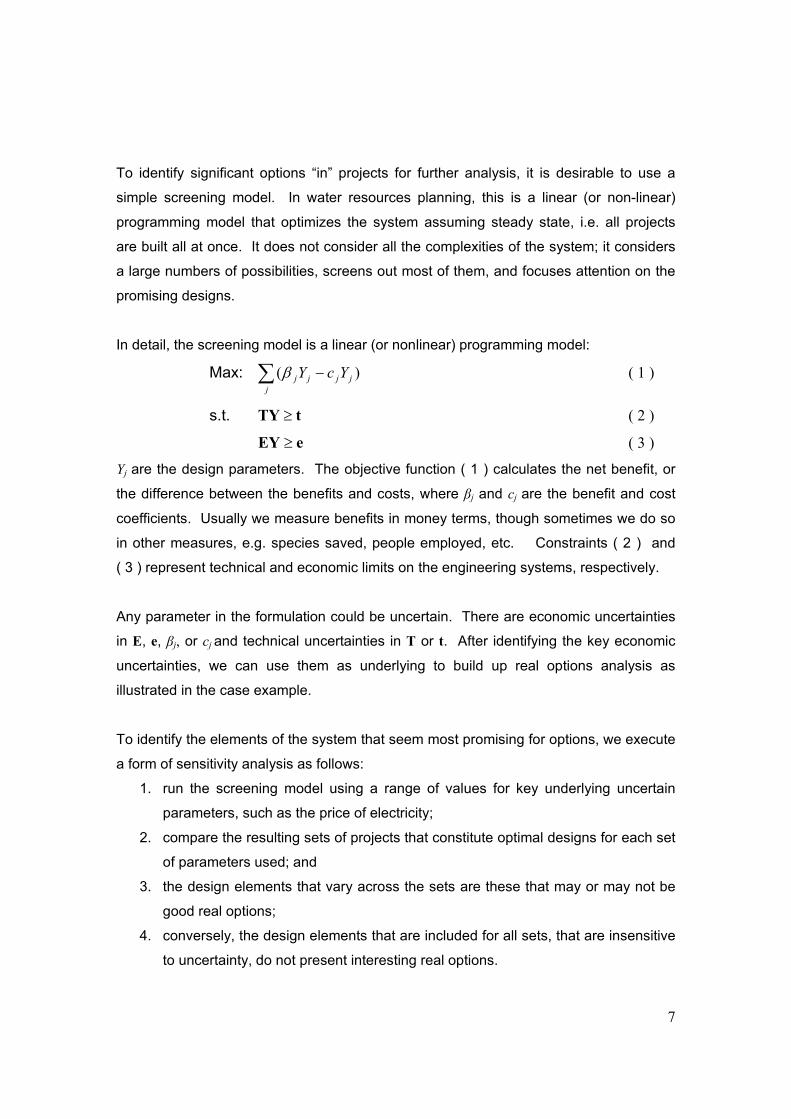
In detail, the screening model is a linear (or nonlinear) programming model:
Max: )(∑ −j
jjjj YcYβ ( 1 )
s.t. tTY ≥ ( 2 )
eEY ≥ ( 3 )
Yj are the design parameters. The objective function ( 1 ) calculates the net benefit, or
the difference between the benefits and costs, where βj and cj are the benefit and cost
coefficients. Usually we measure benefits in money terms, though sometimes we do so
in other measures, e.g. species saved, people employed, etc. Constraints ( 2 ) and
( 3 ) represent technical and economic limits on the engineering systems, respectively.
Any parameter in the formulation could be uncertain. There are economic uncertainties
in E, e, βj, or cj and technical uncertainties in T or t. After identifying the key economic
uncertainties, we can use them as underlying to build up real options analysis as
illustrated in the case example.
To identify the elements of the system that seem most promising for options, we execute
a form of sensitivity analysis as follows:
1. run the screening model using a range of values for key underlying uncertain
parameters, such as the price of electricity;
2. compare the resulting sets of projects that constitute optimal designs for each set
of parameters used; and
3. the design elements that vary across the sets are these that may or may not be
good real options;
4. conversely, the design elements that are included for all sets, that are insensitive
to uncertainty, do not present interesting real options.

8
Simulation model
The simulation model tests several candidate designs from runs of the screening model.
Its main purpose is to examine, under technical and economic uncertainties, the
robustness and reliability of the designs, as well as their expected benefits from the
designs. Such extensive testing is hard to do using the screening model. After using the
simulation model, we find a most satisfactory configuration with design parameters
),...,,( 21 jYYY in preparation for the options analysis.
In standard water resources planning, the simulation model involves many years of
simulated stochastic variation of the water flows, generated on the basis of historical
records. This process leads to a refinement of the designs identified by the screening
model. For the analysis of real options “in” water resources systems, we propose to
modify this standard simulation process. Specifically, we will simulate the combined
effect of stochastic variation of hydrologic and economic uncertain parameters.
If the time series of the water flow consisted of the seasonal means repeating
themselves year after year (no shortages with regard to the design obtained by the
screening model) and the price of electricity were not changing, the simulation model
should provide the same results as the screening model. But the natural variability of
water flow and electricity price will make the result (net benefit) of each run different, and
the average net benefit is not going to be the same as the result from the screening
model. The simulated results should be lower because the designs are not going to
benefit from excess water when water is more than the reservoir can store. Thus
occasional high levels of water do not provide compensation for lost revenues by
occasional low levels of water. Due to these uncertainties, the economies of scale
seemingly apparent under deterministic schemes are reduced.
Options analysis After identifying the most promising real options “in” projects, designers need a model
that enables them to value the set of options and develop a contingency strategy for their
exercise. In contrast to standard financial options analysis, more characteristics are

9
required for the analysis of real options “in” projects, such as technical details and
interdependency/path-dependency among options.
This paper proposes a model based on the scenarios established by a binomial lattice.
In essence, it proposes a new way to look at the binomial tree, recasting it in the form of
a stochastic mixed-integer programming model. The idea is to:
Maximize: binomial tree
Subject to: constraints consisting of 0-1 integer variables representing the
exercise of the options (= 0 if not exercised, =1 if exercised)
Appendix I illustrates the use of this model to value binomial lattices. Such formulation is
unnecessarily complicated for a simple financial option. But for complex and highly
interdependent real options “in” projects, we can specify the relationship of options using
the 0-1 integer variable constraints. Without integer programming, a binomial tree for a
path-dependent real option “in” projects may be too messy to build. With technical,
budget, and real options constraints, a stochastic mixed-integer programming model
accounts for highly complex and interdependent issues, and delivers both a valuation of
the options and a contingency strategy.
Stochastic mixed-integer programming and real options constraints
This section develops a general formulation for the analysis of real options “in” projects,
especially these with path-dependency.
The stochastic mixed-integer programming assumes that the economic uncertain
parameters in E, e, βj, or cj in objective function ( 1 ) and constraints ( 2 ) and ( 3 ) evolve
as discrete time stochastic processes with a finite probability space. A scenario tree is
used to represent the evolution of an uncertain parameter [Ahmed, King, and Parija,
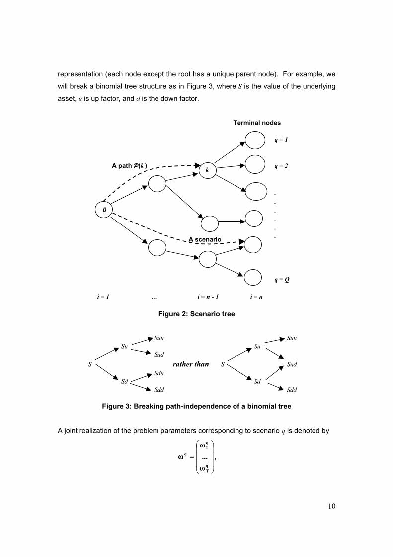
2003]. Figure 2 illustrates the notation. The nodes k in all time stages i constitute the
states of the world. iδ denotes the set of nodes corresponding to time stage i. The path
from the root node 0 at the first stage to a node k is denoted by P(k). Any node k in the
last stage n is a terminal node. The path P(k) to a terminal node represents a scenario,
a realization over all periods from 1 to the last stage n. The number of terminal nodes Q
corresponds to all Q scenarios. Note there is no recombination structure in this tree
10
representation (each node except the root has a unique parent node). For example, we
will break a binomial tree structure as in Figure 3, where S is the value of the underlying
asset, u is up factor, and d is the down factor.
Terminal nodes
q = 1
A path P(k ) q = 2
.
.
.
.
.
.
q = Q
i = 1 … i = n - 1 i = n
0
k
A scenario
Figure 2: Scenario tree
Suu SuuSu Su
SudS rather than S Sud
SduSd Sd
Sdd Sdd
Figure 3: Breaking path-independence of a binomial tree
A joint realization of the problem parameters corresponding to scenario q is denoted by
=qT
q1
q
ω...ω
ω ,

11
where qiω is the vector consisting of all the uncertain parameters for time stage i in
scenario q. pq denotes the probability for a scenario q. The real options decision
variables corresponding to scenario q is denoted by
=qT
q
R
R...
1qR ,
where qiR is the decision on the option at time stage i in scenario q. 0 denotes no
exercise and 1 denotes exercise.
At any intermediate stage i, the decision maker cannot distinguish between any scenario
passing through the same node and proceeding on to different terminal node, because
the state can only be distinguished by information available up to time stage.
Consequently, the feasible solution qiR must satisfy:
21 qi
qi RR = nikkqq i ,...,1,, node through ),( 21 =∀∈∀∀ δ
where q1 and q2 represent two different scenarios. These constraints are known as non-anticipativity constraints.
To illustrate the use of the above approach, we apply it to some standard financial
options. The formulation is:
Max )( )1(
1∑ ∑ −⋅∆⋅−
=
⋅⋅⋅q
iTrT
i
qi
qi
q eREp ( 4 )
s.t. KSE qi
qi −= (American call) or q
iqi SKE −= (American put) qi,∀ ( 5 )
∑ ≤i
qiR 1 q∀ ( 6 )
21 qi
qi RR = nikkqq i ,...,1,, node through ),( 21 =∀∈∀∀ δ ( 7 )
}1,0{∈qiR qi,∀ ( 8 )
where qiS is the value of underlying asset at time stage i in scenario q, K is the exercise
price, r is the risk-free interest rate, and ∆T is the time interval between two consecutive
stages.

12
The objective function ( 4 ) is the expected value of the option along all scenarios.
Constraint ( 5 ) can be any equations that specify the exercise condition. Constraint ( 6 )
makes sure that any option can only be exercised at most once in any scenario.
Constraint ( 7 ) are the non-anticipativity constraints. We call constraints ( 6 ) and ( 7 )
real options constraints.
To illustrate and validate the above formulation, consider an example of an American put
option without dividend payment. For this case, unlike similar call options, it may be
optimal to exercise before the last period. The variables for this example are S = $20, K
= $18, r = 5% per year, σ = 30%, ∆T = 1 year, and time to maturity T = 3 years. Up factor
u = 1.35, down factor d = 0.74. A standard binomial lattice gives the value of the options
as $2.20 as in Table 1.
Now considering the reformulated problem according to equations ( 4 ) to ( 8 ). Solve it
using GAMS©, the maximum value of the objective function is also 2.20. The optimal
solution of 0-1 variables is shown in Table 2. Since 1 means exercise, the result exactly
corresponds to that of the ordinary binomial tree (Table 1). Note there is an exercise in
scenarios 7 and 8 that is not at the last time point. This means the formulation can
successfully find out early exercise points and define contingency plans for decision
makers.
Table 1: Binomial tree for the example American put Period 1 Period 2 Period 3 Period 4Stock Price 20.00 27.00 36.44 49.19Exercise Value -2.00 -9.00 -18.44 -31.19Hold Value 2.20 0.69 0.00 0.00Option Value 2.20 0.69 0.00 0.00Exercise or not? No No No No
Stock Price 14.82 20.00 27.00Exercise Value 3.18 -2.00 -9.00Hold Value 4.00 1.48 0.00Option Value 4.00 1.48 0.00Exercise or not? No No No
Stock Price 10.98 14.82Exercise Value 7.02 3.18Hold Value 6.15 0.00Option Value 7.02 3.18Exercise or not? Yes Yes
Stock Price 8.13Exercise Value 9.87Hold Value 0.00Option Value 9.87Exercise or not? Yes

13
Table 2: Stochastic programming result for the example American put
Stock Price Realization Decision Scenario i = 1 i = 2 i = 3 i = 4 Probability i = 1 i = 2 i = 3 i = 4
q = 1 S Su Suu Suuu 0.132 0 0 0 0 q = 2 S Su Suu Suud 0.127 0 0 0 0 q = 3 S Su Sud Sudu 0.127 0 0 0 0 q = 4 S Su Sud Sudd 0.123 0 0 0 1 q = 5 S Sd Sdu Sduu 0.127 0 0 0 0 q = 6 S Sd Sdu Sdud 0.123 0 0 0 1 q = 7 S Sd Sdd Sddu 0.123 0 0 1 0 q = 8 S Ds Sdd Sddd 0.118 0 0 1 0
Formulation for the real options timing model
The stochastic mixed-integer programming reformulation is much more complicated than
a simple binomial lattice. It is like using a missile to hit a mosquito to value ordinary
financial options. But such reformulations empower analysis of complex path-dependent
real options “in” projects for engineering systems.
Technical constraints in the screening model are modified in the real options timing
model. Since the screening and simulation models have identified the configuration of
design parameters, these are no longer treated as decision variables. On the other hand,
the timing model relaxes the assumption of the screening model that the projects are
built together all at once. It decides the possible sequences of the construction of each
project in the most satisfactory designs for the actual evolution of the uncertain future.
Y is the most satisfactory configuration of design parameters obtained by the “options
identification” stage, it is a vector ),...,,( 21 jYYY corresponding to j design parameters.
The real options decision variable corresponding to scenario q is expanded to:
=qij
qi
qj
q
RR
RR
...::
...
1
111qR , }1,0{∈q
ijR

14
qijR denotes the decision on whether to build the feature according to jth design
parameter for ith time stage in scenario q. The objective function ( 1 ) corresponding to
scenario q is denoted by )(⋅qf . qp and )(⋅qf are derived from the specific scenario tree
based on the appropriate stochastic process for the subject under study. The real
options constraints ( 6 ) to ( 7 ) are concisely denoted by φ. Most importantly, the
objective function is modified to get the expected value along all scenarios.
The real options timing model formulation is as follows.
Max )(∑ ⋅q
qq fp Y,Rq
s.t. tT ≥
qijj
qi
RY
RY:
11
and eE ≥
qijj
qi
RY
RY:
11
iq,∀
ϕ∈qR
}1,0{∈qijR jiq ,,∀
In short, the formulation has an objective function averaged over all the scenarios,
subject to three kinds of constraints: technical, economic, and real options. By
specifying the interdependencies by constraints, we can take into account highly
complex relationship among projects.
Case study: Development of river-run hydropower stations The case example concerns the development of a river basin involving decisions to build
dams and hydropower stations in China. The developmental objective is mainly hydro-
electricity production. Irrigation and other considerations are secondary because the
river basin is in a remote and barren place.
Screening model
The screening model identifies initial configurations of design parameters for the river
basin development, which are sites, reservoir storage capacity, and installed electricity
generation capacity. The objective function is to maximize the net present value (NPV)

15
from the river basin development projects. The constraints include water continuity,
reservoir storage capacity, hydropower production, and budget constraints. See
Appendix II for details.
The key uncertain economic parameter here is the price of electricity, which may vary
dramatically as China develops economically and moves toward market determination of
prices. We should account carefully for this critical uncertain element in planning. If we
optimize using expected electricity price, the problem usually leads to economies of
scale arguments indicating that bigger is better. Unfortunately, given the uncertain
economic elements, in many cases it does not pay to build as big as possible by
exploiting economies of scale, since the demand is often insufficient to justify the biggest
capacity. It may well be more attractive to build smaller projects with options thinking
[Mittal, 2004]. This reality is a prime motive for studying real options in large-scale
engineering systems. To identify the options worth investigating due to the uncertainty
of electricity price, we run the screening model with different electricity prices ranging
around the estimated current price of 0.25 RMB/KwH.
This example screening model involves 3 sites and 2 seasons. According to practice, it
is run for a typical year with mean water flows for the dry and wet seasons, implying that
all years are the same by setting the initial storage of season 1 equal to the final storage
of season 2. (Once the screening model has determined optimal designs of the system,
and thus reduced the number of variables, the subsequent simulation and timing models
introduce the stochastic elements. This strategy allocates computational effort to where
it is most productive.)
This example screening model involves 46 variables and 58 constraints. It contains only
the most important considerations, yet has a fair amount of technical details, and shows
how complex the interdependencies among real options “in” projects for large-scale
engineering systems can be.
The optimization model was written in GAMS©, and the results are as in Table 3.
“Optimal value” represents the optimal net benefit calculated by the objective function.
Vs and Hs represent the reservoir storage capacity and the installed electricity generation
capacity for site s. Note that for the first site, the design with reservoir storage capacity

16
of 9600×106 m3 and installed electricity generation capacity of 3600 MW is robust since it
is the best choice for any price scheme except when the price is extremely low. For the
other two sites, the optimal design depends on the price of electricity. For case 1, no
projects are built; for cases 2 and 3, site 3 is screened out. In a real application
considering many more sites, there may be a great number of sites entered the
screening models and most of them are screened out. Although current electricity price
was 0.25 RMB/KwH at the time of the study, we cannot assume that the design that
corresponds to this price is optimal, because this screening model does not consider the
uncertainty of electricity price. Follow-on analysis is needed.
Table 3: Results from the screening model
Case Electricity Price
(RMB/KwH)
H1
(MW)
V1
(106m3)
H2
(MW)
V2
(106m3)
H3
(MW)
V3
(106m3)
Optimal Value (106RMB)
1 0.09 0 0 0 0 0 0 0
2 0.12 3600 9600 1700 25 0 0 367
3 0.15 3600 9600 1700 25 0 0 796
4 0.18 3600 9600 1700 25 1564 6593 853
5 0.22 3600 9600 1700 25 1723 9593 1607
6 0.25 3600 9600 1700 25 1946 12242 2196
7 0.28 3600 9600 1700 25 1966 12500 2796
8 0.31 3600 9600 1700 25 1966 12500 3396
Simulation model
The example simulation model introduces stochastic considerations, both in electricity
price and in seasonal flows. In that respect, it uses 60 years of 6-month flows to account
for the aspects of over year storage not considered in the screening model. Using the
simulation model reveals more aspects of the designs chosen by the screening model,
especially the hydrologic reliability. The example simulation model does not look into the
hydrologic reliability issue deeply, because its main purpose is to validate the
identification of the real options.
The simulation model was constructed using Excel© and Crystal Ball©. All designs from
the screening model in Table 3 were tested. The optimal design by the screening model

17
that corresponds to the current electricity price of 0.25 RMB/KwH is not necessarily the
best design after various uncertainties enter the picture.
For cases 5 and 6 (electricity price = 0.22 RMB/KwH and 0.25 RMB/KwH), the
simulation results are as Figure 4. Note that the expected NPV in both cases are
substantially below those indicated in Table 3 (1138 vs. 1607 for case 5; 1098 vs. 2196
for case 6). As indicated before, this result is not unexpected since higher capacity
designs often cannot be fully used (due to lower flows) yet cannot take advantage of
higher flows (due to limited capacity). Note also that the lower capacity design (case 5)
provides higher expected NPV than the higher capacity design (case 6) that appeared
better in the deterministic design. This is a common, but not necessary, result.
The final design chosen is the design for case 5. It was analyzed further using real
options “in” projects timing model. Each project in the design is an option. We have the
right but not obligation to exercise it; in other words, we can choose whether to build a
project at a specific time.
Frequency Chart
Mean = 1138 .000
.009
.019
.028
.037
0
23.25
46.5
69.75
93
-1086 441 1969 3496 5024
2,500 Trials 0 Outliers Forecast: Net Benefits
Figure 4a: Simulation result for electricity price = 0.22 RMB/KwH (case 5)
Frequency Chart
Mean = 1098 .000
.008
.016
.024
.032
0
20
40
60
80
-968 417 1801 3185 4569
2,500 Trials 0 Outliers Forecast: Net Benefits
Figure 4b: Simulation result for electricity price = 0.25 RMB/KwH (case 6)

18
Real options timing model
After applying the screening and simulation models, the next step is to relax their
assumption that all projects are built at once, and study the development process from
no project onwards. The key issues in the real options timing model is the order and
timing of the construction of the projects, given various constraints.
The example real options timing model assumes that projects can be constructed during
3 time periods of 10 years. The calculation considers a 70-year life for each project.
As a baseline, consider the result of the timing model when the electricity price is
deterministic, that is, when we do not consider the real options. (The Use of GAMS© to
solve the timing model without real options considerations as described in Appendix III.)
The timing model takes into account the transition process that projects, once built,
gradually increase the production to full capacity. It recognizes that it takes time to build
reservoirs and power plants and to fill up reservoirs. This deferral of benefits over many
years has a huge impact on the NPV for large, capital-intensive projects. Thus, projects
that appeared good in the screening or simulation model analyses may turn out to be
less attractive when timing issues are considered.
The real options timing model incorporates uncertainty in the hydropower benefit
coefficient (energy price). It gives a contingency plan in reaction to the actual realization
of energy price. In this connection, we would again like to point out the path-dependent
feature of this problem. Refer to Figure 3. For example, in the second stage, if electricity
price goes up, a project is built; but if it goes down, no project is built. According to the
formula for binomial tree, the middle point of the third stage has a price of Sud or Sdu,
numerically the same, however, it is different for the following two paths leading into the
point because of the hydrological conditions: first path, the price goes up in the second
stage, and goes down the third stage with a project changing the water flow; the second
path, the price goes down in the second stage, and goes up in the third stage with no
project and the natural water flow.
For the example analysis, the movement of electricity price is assumed to follow a
geometric Brownian motion (GBM). This is not necessarily the best model for electricity
price: a mean-reverting proportional volatility model might improve the quality of analysis

19
[Bodily and Del Buono, 2002]. However, GBM is sufficient to illustrate the analysis
framework and stochastic mixed-integer programming methodology. To use a different
stochastic process, we only need to generate an appropriate scenario tree, and the
analysis framework remains valid. In this example, we use the volatility of electricity
price as %96.6=eσ , its current electricity price as 0.25 RMB/KwH, and its drift rate as µ
= –0.33% per year [Wang, 2003].
Compared to the timing model without real options considerations (Appendix III), the
objective of the real options timing model is changed to:
Max ∑∑∑
∑∑ ∑∑ ∑ ∑∑∑∑
⋅+−
+−−=
s q ii
qisssss
q
s q i t
i
j s q i t
qisiist
qPT
qi
qis
qjsist
qPi
q
PVCRHVp
RPVOPpPVRfRPp
})]()({[
])1([1
δα
ββ
where
∑+−= +
=i
ijji r
PV10
1)1(10 )1(1
∑= +
=70
31 )1(1
jjo r
PV
)1(10)1(1
−+= ii r
PVC
Likewise, the constraints differ because this formulation adds the real options constraints:
∑ ≤i
qisR 1
qs,∀
21 qis
qis RR = nikkqq i ,...,1,, node through ),( 21 =∀∈∀∀ δ
Using GAMS©, we obtain the results for the real options timing model as Table 4. For
example, for the first scenario q = 1 that occurs with probability = 0.138: the electricity
prices for the first, second, and third 10-year time period (i = 1, 2, and 3) are 0.250,
0.312, and 0.388 RMB/KwH, respectively. The real options decision variables for Project
2 in the first period and Project 1 in the third period are 1’s, and the other 7 real options
decision variables are 0’s (we have 9 real options decision variables for each scenario, 3
projects times 3 periods each). Therefore, for scenario 1, the decision is to build Project

20
2 in the first period and Project 1 in the third period. The rest of Table 4 can be read in
the same way. In summary, as in Figure 5, the optimal strategy or contingency plan is to
build Project 2 in the first time stage whatever the electricity price is. And build nothing
in the second stage. In the last stage, we only build Project 1 in the case that price is up
for the second stage and up again for the third stage, for other cases, we build nothing.
Table 4: Results for real options “in” projects timing model (Current electricity price 0.25 RMB/KwH)
Electricity Price Realization Decision
Scenario i = 1 i = 2 i = 3 Prob i = 1 i = 2 i = 3Project 1 0 0 1 Project 2 1 0 0 q = 1 0.250 0.312 0.388 0.138Project 3 0 0 0 Project 1 0 0 0 Project 2 1 0 0 q = 2 0.250 0.312 0.250 0.233Project 3 0 0 0 Project 1 0 0 0 Project 2 1 0 0 q = 3 0.250 0.201 0.250 0.233Project 3 0 0 0 Project 1 0 0 0 Project 2 1 0 0 q = 4 0.250 0.201 0.161 0.395Project 3 0 0 0
The overall expected net benefit is 4345 Million RMB. This is almost 4 times bigger than
the simulation result in Figure 4a. There are two reasons for it:
1. Timing model can eliminate the unprofitable projects, while the simulation model
cannot. As a comparison, the timing model without real options considerations
as in Appendix III suggests that only project 2 should be built in the first time
period and that projects 1 and 3 should never be built, with an overall expected
net benefit of 4239 million RMB.
2. Real options add additional value by building project 1 in favorable situation
(electricity price high) and avoiding it in unfavorable situation (electricity price
low). Refer to Figure 5. In this example, the added value is not enormous, but
the principle is established.
.

21
Price = 0.388 RMB/KwHProject 1 build
Project 3 no build
Price = 0.312 RMB/KwH Price = 0.250 RMB/KwHProject 1 no build Project 1 no build
Price = 0.25 RMB/KwH Project 3 no build Project 3 no buildProject 1 no buildProject 2 build Price = 0.250 RMB/KwH
Project 3 no build Price = 0.201 RMB/KwH Project 1 no buildProject 1 no build Project 3 no buildProject 3 no build
Price = 0.250 RMB/KwHProject 1 no buildProject 3 no build
Figure 5: Contingency plan
There are three important notes regarding the results:
1. This real options timing model provides a contingency plan (as Figure 5)
depending on how events roll out, as well as the value of the system with real
options. Using the real options timing model, we learn to build Project 2 in the
first stage, and build Project 1 in the third stage given certain electricity price
condition; if using the timing model without real options considerations, the
decision is to build Project 2 in the first stage, and then build nothing else, surely
missing something compared to the real options timing model.
2. This contingency plan takes into account the complex interdependencies among
projects, in this case, through the water flows (for example, one dam in the
upstream will store water and help downstream stations to produce more in dry
season). Using conventional options analysis, it is hard to deal with such
interdependencies. This example is simpler than real water resources planning;
nevertheless, we can use exactly the same methodology, with more computation
and other resources, to tackle much more complex real water resources planning
problem.
3. The value of options is the difference between the optimal benefits from the
timing model with and without real options considerations, 106 million RMB.
Note the valuation of real options “in” projects looks not for an exact numeric
result as valuation of financial options, but assesses whether flexible designs are
worth. The cost to get the real options “in” projects is usually 0 as in this case
study. This process about real options valuation is more about the process of
designing flexibility itself rather than a specific value of optimal benefit.

22
Before we finish our analysis, let us see how the optionality of the plan can be more
significant if the current electricity price is higher. If we take the current electricity price
as 0.30 RMB, the result is as Table 5. The contingency plan is to build Project 2 in the
first stage, build Project 1 in the second stage if the price goes up, build Project 3 in the
third stage if the price goes up both in the second and third stage. Refer to Figure 6.
Note the path-dependent feature: in the third stage, for the same electricity price of 0.30
RMB/KwH, Project 1 can have been built or not, depending whether the electricity price
in the second stage were high or low.
Table 5: Results for real options “in” projects timing model (Current electricity price taken to be 0.30 RMB/KwH)
Electricity Price Realization Decision Scenario i = 1 i = 2 i = 3 Prob i = 1 i = 2 i = 3
Project 1 0 1 0 Project 2 1 0 0 q = 1 0.300 0.374 0.466 0.138 Project 3 0 0 1 Project 1 0 1 0 Project 2 1 0 0 q = 2 0.300 0.374 0.300 0.233 Project 3 0 0 0 Project 1 0 0 0 Project 2 1 0 0 q = 3 0.300 0.241 0.300 0.233 Project 3 0 0 0 Project 1 0 0 0 Project 2 1 0 0 q = 4 0.300 0.241 0.193 0.395 Project 3 0 0 0
Price = 0.466 RMB/KwH
Project 3 buildPrice = 0.374 RMB/KwH
Project 1 build Price = 0.300 RMB/KwHPrice = 0.300 RMB/KwH Project 3 no build Project 3 no build
Project 1 no buildProject 2 build Price = 0.300 RMB/KwH
Project 3 no build Price = 0.241 RMB/KwH Project 1 no buildProject 1 no build Project 3 no buildProject 3 no build
Price = 0.193 RMB/KwHProject 1 no buildProject 3 no build
Figure 6: Contingency plan (if current electricity price = 0.30 RMB/KwH)

23
Computational issues A key consideration in solving a stochastic mixed-integer programming is whether a
result is a global or local optimum. It is not simple to prove the result of an integer
programming problem is a global optimum. And it may be hard to find a general
solution for the real options timing model because of the special structure of the
technical and economic constraints. Nevertheless, integer programming improves
solutions to highly complex and interdependent real options that cannot be solved by
ordinary binomial trees. When there is no dependency among nodes, it is possible to
optimize on each node and roll back to get the option value. When dependency exists,
this simple approach no longer works. A stochastic mixed-integer programming at least
provides a local optimum better than the results from conventional approaches or human
intuition.
Finally, a few words about the computational costs: for the example river basin
development problem, the number of variables is 187, of which 36 are 0-1 discrete
variables, and the number of constraints is 261. It takes a laptop (PIII 650, 192M RAM)
less than 2 seconds to use GAMS© to figure out a solution.
Conclusion By proposing a new way to formulate real options “in” projects, this paper attacks the
possibility of building real options into the design of the physical facilities themselves.
This generalizable solution will improve the design and planning of large engineering
systems, such as manufacturing systems, commercial satellite systems, and logistics
systems. It is not only in the sense of designing with full awareness of uncertainties, but
also how to design options (flexibility) into systems to proactively manage inevitable
uncertainties.
Three most important points in the paper are:
two stage analysis, identifying the most interesting real options “in” projects
before analyzing them;
using stochastic mixed-integer programming to value real options as well as to
find a contingency plan for excising the options. In the stochastic mixed-integer
programming formulation, there are real options constraints added onto technical

24
constraints and economic constraints. Highly complex interdependencies among
options can be specified using constraints; and
focusing on developing the most appropriate design of system flexibility and
building up suitable contingency plan for dealing with future uncertainties, rather
than valuing individual options.
Acknowledgements
The authors deeply appreciate the guidance of Denis McLaughlin and Gordon Kaufman
in the formulation of this work, and anonymous Chinese friends for providing details to
support the case study.
References Ahmed, S., King, A.J., and Parija, G. (2003) “A Multi-stage Stochastic Integer
Programming Approach for Capacity Expansion under Uncertainty,” Journal of Global
Optimization 26, pp. 3 – 24.
Bertsimas, D. and Tsitsiklis, J. (1997) Introduction to Linear Programming, Athena
Scientific, Belmont, MA.
Birge, J.R. and Louveaux, F. (1997) Introduction to Stochastic Programming. Springer,
New York, NY.
Bodily, S and Del Buono, M. (2002) “Risk and Reward at the speed of Light: A New
Electricity Price Model,” Energy Power Risk Management, Sept., pp. 66 –71.
Cortazar, G. and Casassus, J. (1997) “A Compound Option Model for Evaluating
Multistage Natural Resource Investment,” in Project Flexibility, Agency, and Competition
(2000) pp. 205 - 223, edited by Brennan, M. and Trigeorgis, L., Oxford University Press,
New York, NY.
Copeland, T.E. and Antikarov, V. (2001) Real Options - A Practitioner's Guide, TEXERE,
New York, NY.
Cox, J., Ross, S., and Rubinstein, M. (1979) “Option Pricing: A Simplified Approach,”
Journal of Financial Economics, 7, pp. 263 - 384.
de Neufville, R. (2002) Class notes for Engineering Systems Analysis for Design, MIT
engineering school-wide elective, Cambridge, MA.

25
de Neufville, R. et al. (2004) ”Uncertainty Management for Engineering Systems
Planning and Design.” Monograph, Engineering Systems Symposium, MIT, Cambridge,
MA. March. http://esd.mit.edu/symposium/pdfs/monograph/uncertainty.pdf
de Weck, O. et al. (2004) “Staged Deployment of Communications Satellite
Constellations in Low Earth Orbit," Journal of Aerospace Computing, Information, and
Communication, March, pp. 119-136.
Geske, R. (1979) “The valuation of compound options,” Journal of Financial Economics,
March, pp. 63 - 81.
Goldberg, R and Read, J (2000) “Dealing with a Price-Spike World,” Energy and Power
Risk Management, May, pp. 39 – 41.
Luenberger, D. (1998) Investment Science, Oxford University Press, New York, NY.
Major, D. and Lenton, L. (1979) Applied Water Resource Systems Planning, Prentice-
Hall, Englewood Cliffs, NJ.
Mittal, G. (2004) “Real Options Approach to Capacity Planning under Uncertainty,”
Master of Science Thesis, Department of Civil and Environmental Engineering, MIT,
Cambridge, MA.
Oueslati, S.K. (1999) “Evaluation of Nested and Parallel Real Options: Case Study of
Ford's investment in Fuel Cell Technology,” Master of Science Thesis, Technology and
Policy Program, MIT, Cambridge, MA.
Siegel, D., Smith, J., and Paddock, J. (1987) “Valuing Offshore Oil Properties with
Option Pricing Models,” Midland Corporate Finance Journal, Spring, pp. 22 - 30.
Trigeorgis, L. (1993a) “The Nature of Options Interactions and the Valuation of
Investments with Multiple Options,” Journal of Financial and Quantitative Analysis,
Spring, pp. 1 - 20.
Trigeorgis, L. (1993b) “Real Options and Interactions with Financial Flexibility,” Financial
Management, Autumn, pp. 202 - 224.
Wang, T. (2003) “Analysis of Real Options in Hydropower Construction Projects: A Case
Study in China,” Master of Science Thesis, Technology and Policy Program, MIT,
Cambridge, MA.

26
Appendix I: Using mixed-integer programming to solve a binomial lattice By simple examples on financial options, we would illustrate the basic idea of using
stochastic mixed-integer programming model to value options.
Important variables for options valuation are as follows
S: Current Stock Price
K: Exercise Price
T: Time to Expiration
r: Risk free interest rate
σ: Volatility
∆T: Time interval between nodes
Important Formulas for Binomial Tree Model include:
dudep
ed
eu
Tr
T
T
−−
=
=
=
∆
∆−
∆
σ
σ
On each node of a binomial tree, the calculation is as Table 6. Note this is for the
valuation of American options, and p is risk-neutral probability.
Table 6: Decision on each node of a binomial lattice
Stock Price S Exercise Value S – K (for call); K – S (for put) Hold Value
rdu
epdownpriceifValueOptionpuppriceifValueOption ⋅+⋅ ________
Options Value Max (Exercise Value, Hold Value) (0 for the last period)
Now we will compare an ordinary binomial tree and an integer programming binomial
tree. The interesting part is to compare the option value from the binomial tree and the
optimal value from the integer programming, as well as the “exercise or not” result for
each node of the binomial tree and the value of 0-1 integer variables in the optimal

27
solution of the integer programming. The American option is of special interest because
we want to examine if the integer programming can correctly identify the case of early
exercise before the last period.
For example, the parameters for an American call option are S = $20, K = $21, T = 3
years, r = 5% per year, σ = 30%, ∆T = 1 year. The binomial tree is as Table 7, and the
value of the options is $5.19.
Table 7: Binomial tree for the American call option Period 1 Period 2 Period 3 Period 4 Stock Price 20.00 27.00 36.44 49.19 Exercise Value -1.00 6.00 15.44 28.19 Hold Value 5.19 9.34 16.47 0.00 Option Value 5.19 9.34 16.47 28.19 Exercise or not? No No No Yes
Stock Price 14.82 20.00 27.00 Exercise Value -6.18 -1.00 6.00 Hold Value 1.41 2.91 0.00 Option Value 1.41 2.91 6.00 Exercise or not? No No Yes
Stock Price 10.98 14.82 Exercise Value -10.02 -6.18 Hold Value 0.00 0.00 Option Value 0.00 0.00 Exercise or not? No No
Stock Price 8.13 Exercise Value -12.87 Hold Value 0.00 Option Value 0.00 Exercise or not? No
Node 11
Node 21
Node 22
Node 31
Node 32
Node 33
Figure 7: Node representation for a binomial tree

28
Now let us use Integer programming to value this binomial tree. The node im on a
binomial tree is indexed in the following way: i represents the ith stage, m represents the
mth node for a specific stage. Because of the nice feature of recombination of a binomial
tree when there is path independence, the number of nodes at ith time point is exactly i,
so m takes the number from 1 to i. Please refer to Figure 7.
At node im, let imS denote the stock price, imE denote the exercise value, imH denote
the hold value, imV denote the option value, imR be a 0-1 integer variable denoting
whether the option is exercised at node im, 0 is not exercise and 1 is exercise. The
number of stages is n.
The objective function is to get the maximum value of V11 at the beginning node. The
option value imV is specified by
)1( imimimimim RHREV −⋅+⋅=
Since the programming maximizes the value, its final result will satisfy that imV is the
maximum of imE and imH .
The exercise value imE for a call options is
KSE imim −=
The hold value for the last time point is 0, or 0, =mnH . For ni < , the hold value
Trmimi
im epVpV
H ∆⋅+++ −⋅+⋅
=)1(1,1,1
We are using continuous compounding here.
The stock price imS at node im is defined by the following formula
Tmiim eSS ∆−+= σ)21(
11
where 11S is the current stock price.

29
Complete formulation of the integer programming problem is as follows:
Maximize 11V ( 9 )
Subject to )1( imimimimim RHREV −⋅+⋅= imi ,...,1; =∀ ( 10 )
KSE imim −= imi ,...,1; =∀ ( 11 )
Trmimi
im epVpV
H ∆⋅+++ −⋅+⋅
=)1(1,1,1 imni ,...,1;1,...,1 =−= ( 12 )
0, =mnH m∀ ( 13 )
Tmiim eSS ∆−+= σ)21(
11 imi ,...,1; =∀ ( 14 )
Solve the integer programming using GAMS, the maximum value of the objective
function is 5.19. The values for 0-1 integer variables are as Table 8. Since 1 means
exercise, the result is exactly correspondent to the ordinary binomial tree as Table 7.
oo
Table 8: Result of the stochastic programming for the American call option
Rij i = 1 i = 2 i = 3 i = 4 j = 1 0 0 0 1 j = 2 0 0 1 j = 3 0 0 j = 4 0
30
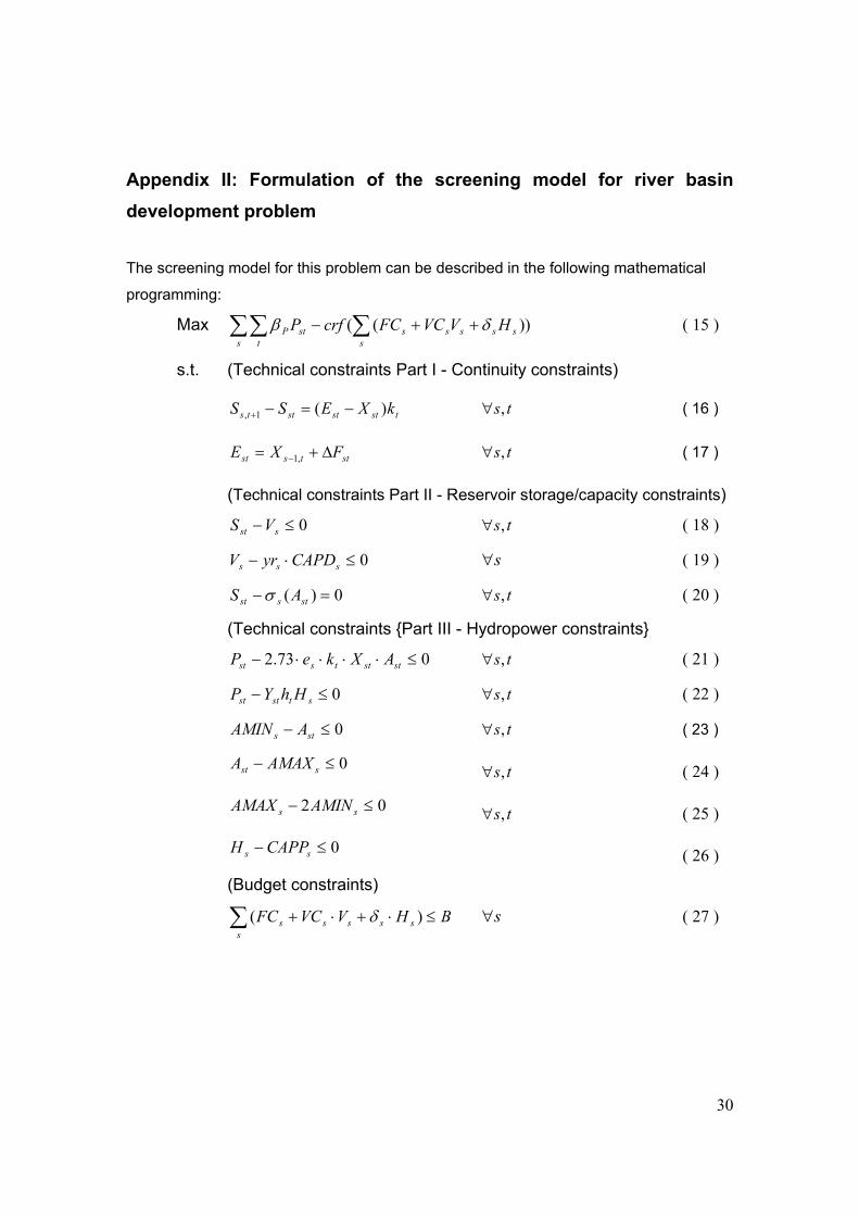
Appendix II: Formulation of the screening model for river basin development problem
The screening model for this problem can be described in the following mathematical
programming:
Max ))(( sss t s
sssstP HVVCFCcrfP δβ ++−∑∑ ∑
( 15 )
s.t. (Technical constraints Part I - Continuity constraints)
tstststts kXESS )(1, −=−+ ts,∀ ( 16 )
sttsst FXE ∆+= − ,1 ts,∀ ( 17 )
(Technical constraints Part II - Reservoir storage/capacity constraints)
0≤− sst VS ts,∀ ( 18 )
0≤⋅− sss CAPDyrV s∀ ( 19 )
0)( =− stsst AS σ ts,∀ ( 20 )
(Technical constraints {Part III - Hydropower constraints}
073.2 ≤⋅⋅⋅⋅− ststtsst AXkeP ts,∀ ( 21 )
0≤− ststst HhYP ts,∀ ( 22 )
0≤− sts AAMIN ts,∀ ( 23 )
0≤− sst AMAXA ts,∀ ( 24 )
02 ≤− ss AMINAMAX ts,∀ ( 25 )
0≤− ss CAPPH ( 26 )
(Budget constraints)
BHVVCFCs
sssss ≤⋅+⋅+∑ )( δ s∀ ( 27 )

31
Table 9: List of Variables for the screening model
Variable Definition Units yrs Integer variable indicating whether or not the reservoir is
constructed at site s
Sst Storage at site s for season t 106m3
Xst Average flow from site s for season t m3/s Est Average flow entering site s for season t m3/s Pst Hydroelectric power produced at site s for season t MwH Ast Head at site s for season t m Hs Capacity of power plant at site s MW VS Capacity of reservoir at site s 106m3
AMAXs Maximum head at site s m AMINs Minimum head at site s m
Table 10: List of Parameters for the screening model
Parameter Definition Units Value Qin,t Upstream inflow for season t m3/s (374,283) CAPDs Maximum feasible storage capacity
at site s 106m3 (9600, 25,
12500) CAPPs Upper bound for power plant
capacity at site s MW ( 3600, 1700,
3200) ∆Fst Increment to flow between sites s
and the next site for season t m3/s (212, 105)
for site 3, others are 0
es Power plant efficiency at site s 0.7 kt Number of seconds in a season Million
Seconds 15.552
ht Number of hours in a season Hours 4320 Yst Power factor at site s for season t 0.35 βP Hydropower benefit coefficient 103 RMB
/MwH 0.25
FCs Fixed cost for reservoir at site s B RMB (11.19,0,8.41)VCs Variable cost for reservoir at site s B
RMB/106m3 (4.49×10⁻⁴, 0, 6.68 ×10⁻⁴)
δs Variable cost for power plant at site s B RMB/MW (7.65×10⁻⁴, 1.85×10⁻³, 8.80 ×10⁻⁴)
r Discount rate 0.086 crf Capital recovery factor for 60 years 0.087 B Total Budget available 103 RMB 80,000,000

32
Above is a simplest version of a river basin planning screening model without losing the
critical considerations, there will be much more details added for real planning. The
objective function
( 15 ) is to maximize the annualized profit from electricity sales.
Technical constraints include continuity constraints, reservoir storage and capacity
constraints, and hydropower constraints. Besides the information from the lists of
variables and parameters (Table 9 and Table 10), several notes: constraint ( 20 )
specifies the relationships between reservoir storage volume and head, they are decided
by specific geological conditions for sites; constant 2.73 in constraint ( 21 ) is a
conversion factor; constraints ( 23 ) to ( 25 ) are to limit marked head variation that is
very inefficient for power production.
The calculation of the conversion factor in constraint ( 21 ) is as follows: Since 1 Joule =
1 N·m (or m2·kg/s2), and per m3 of water weighs 103 Kg, so per m3 of water can generate
103·g power (where g is the acceleration of gravity, equal to 9.81 m/s2). One more issue
to think about is that the energy is counted in MwH, and the time unit in the formulation is
“million seconds”, so we need a conversion factor:
326
6233
73.210min/60min/6010/81.9/10
smhourkg
shoursmmkg ⋅
=⋅⋅⋅⋅

33
Appendix III: Formulation of the timing model without real options considerations
The timing model has almost all 0-1 integer variables except for the flow variables
representing stream flow at different points of the river basin and the energy variables
representing the energy production, while the screening model has most continuous
variables to decide reservoir capacity and power plant sizes that can take any real value
within the constraints. In the timing model, the sizes of the projects have been decided.
The remaining decisions are whether to construct a particular project within a specific
period of time. Such decisions are appropriately represented by integer variables.
The calculation considers 70 years of life for each project. Different time span can be
used, but the difference on results would be small. Complete formulation of the timing
model:
Objective function:
Max })]()({[
][])1([1
∑∑
∑∑∑ ∑∑∑∑
⋅+−
+−−=
i siisssss
i s t s t iisiist
Pi
jiisjsistP
PVCRHV
RPVOPPVRfRP
δα
ββ
Where ∑+−= +
=i
ijji r
PV10
1)1(10 )1(1
∑= +
=70
31 )1(1
jjo r
PV
)1(10)1(1
−+= ii r
PVC
Continuity constraints:
3311
3311,31 i
i
jjini RcRYQX −+= ∑
=
3321
3322,32 i
i
jjini RcRYQX −+= ∑
=

34
∑=
−+∆+=i
jijii RcRYFXX
1112112323212
1121 ii XX ≤
1222 ii XX ≤
Construction constraint:
∑ ≤i
isR 1
Hydropower constraints:
∑=
⋅⋅⋅⋅=i
jjsstisitsist RAXkeP
173.2
0≤− ststist HhFP
Budget constraint:
1≤∑s
isR
Table 11: List of variables for the timing model
Variable Definition Units Xist Average flow from site s for season t for time period i m3/s Pist Hydroelectric power produced at site s for season t for time
period i MwH
Ris 0-1 variable indicating whether or not the project is built at site s for time period i

35
Table 12: List of parameters for the timing model
Parameter Definition Units Values Qin,t Upstream inflow for season t m3/s (374,283) ∆Fst Increment to flow between sites s and
the next site for season t m3/s (389, 154) for site
3, others are 0 es Power plant efficiency at site s 0.7 kt Number of seconds in a season Million
Seconds 15.552
ht Number of hours in a season Hours 4320 Fst Power factor at site s for season t 0.35 βP Hydropower benefit coefficient 103 RMB
/MwH 0.25
βPi Hydropower benefit coefficient for time stage i in the real options timing model
FCs Fixed cost for reservoir at site s B RMB (11.19,0,8.41) VCs Variable cost for reservoir at site s B
RMB/106m3(4.49×10-4, 0, 6.68 ×10⁻⁴)
sH Capacity of power plant at site s MW (3600, 1700, 1723)
sV Capacity of reservoir at site s 106m3 (9600, 0, 9593)
stA Head at site s for season t m (262, 262; 280, 280; 240, 253)
stY Reservoir yield at site s for season t (the change of the flow if a reservoir is built)
m3/s (0, 0; 0, 0; -63.6, 63.6)
stc Part of flow at site s season t to be used in the construction period to ensure a full reservoir of the next period
m3/s 0
f The ratio of average yearly power production during the construction period over the normal production level
0.226
δs Variable cost for power plant at site s B RMB/MW
(7.65×10⁻⁴, 1.85×10⁻³, 8.80 ×10⁻⁴)
PVi Factor to bring 10-year annuity of benefit back to the present value as of year 0 (now)
(6.532, 2.863, 1.254)
PVOi Factor to bring the annuity from year 31 to year 70 back to year 0
(0.896, 0.943, 0.963)
PVCi Factor to bring cost in the ith period back to year 0
(1, 0.438, 0.192)
r Discount rate 0.086
syr Indicating whether or not the project is built at site s
(1, 1, 1)
crf Capital recovery factor 0.087