rna$seq(dataanalysis(tutorial(physiology.med.cornell.edu/.../2015/...sboner.pdf ·...

RNA-‐seq data analysis tutorial

Andrea Sboner 2015-‐05-‐21

NGS Experiment

Data management:

Mapping the reads CreaCng summaries

Downstream analysis: the interes)ng stuff DifferenCal expression, chimeric transcripts, novel transcribed regions, etc.

What is RNA-‐seq?

•  Next-‐generaCon sequencing applied to the “transcriptome” ApplicaCons:

Gene (exon, isoform) expression esCmaCon Differen)al gene (exon, isoform) expression analysis Discovery of novel transcribed regions Discovery/Detec)on of chimeric transcripts Allele specific expression …

NGS Experiment

Data management:



QC and pre-‐processing •  First step in QC:

–  Look at quality scores to see if sequencing was successful

•  Sequence data usually stored in FASTQ format:

@BI:080831_SL-XAN_0004_30BV1AAXX:8:1:731:1429#0/1 GTTTCAACGGGTGTTGGAATCCACACCAAACAATGGCTACCTCTATCACCC + hbhhP_Z\[`VFhHNU]KTWPHHIKMIIJKDJGGJGEDECDCGCABEAFEB

Header (typically w/ flowcell #) Sequence

Quality scores

flow cell lane Cle number x-‐coordinate y-‐coordinate provided by user 1st end of paired read

40,34,40,40,16,31,26,28,27,32,22,6,40,8,14,21,29,11,20,23,16,…

ASCII table

Numerical quality scores

Typical range of quality scores: 0 ~ 40

Freely available tools for QC •  FastQC

–  hep://www.bioinformaCcs.bbsrc.ac.uk/projects/fastqc/ –  Nice GUI and command line interface

•  FASTX-‐Toolkit –  hep://hannonlab.cshl.edu/fastx_toolkit/index.html –  Tools for QC as well as trimming reads, removing adapters, filtering by read quality, etc.

•  Galaxy –  hep://main.g2.bx.psu.edu/ –  Web interface –  Many funcCons but analyses are done on remote server

FastQC •  GUI mode

fastqc

•  Command line mode

fastqc fastq_files –o output_directory – will create fastq_file_fastqc.zip in output directory

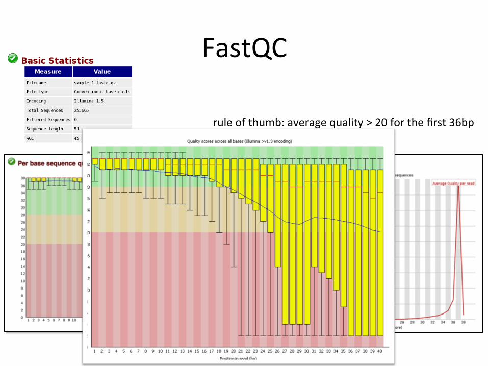
FastQC

read 1

rule of thumb: average quality > 20 for the first 36bp

-‐ median -‐ mean

What to do when quality is poor? •  Trim the reads

•  FASTX-‐toolkit –  fastx_trimmer

–f N –l N

–  fastq_quality_filter -‐q N –p N

–  Fastx_clipper -‐a ADAPTER

NGS Experiment

Data management:



Mapping InsCtute for ComputaConal Biomedicine

Mapping ATCCAGCATTCGCGAAGTCGTA

Mapping to a reference

•  Genome •  Transcriptome •  Genome + Transcriptome •  Transcriptome + Genome •  Genome + splice juncCon library

reference transcriptome

Alignment tools •  BWA

–  hep://bio-‐bwa.sourceforge.net/bwa.shtml –  Gapped alignments (good for indel detecCon)

•  BowCe –  hep://bowCe-‐bio.sourceforge.net/index.shtml –  Supports gapped alignments in latest version (bowCe 2)

•  TopHat –  hep://tophat.cbcb.umd.edu/ –  Good for discovering novel transcripts in RNA-‐seq data –  Builds exon models and splice juncCons de novo. –  Requires more CPU Cme and disk space

•  STAR –  heps://code.google.com/p/rna-‐star/ –  Detects splice juncCons de novo –  Super fast: ~10min for 200M reads but –  Requires 21Gb of memory

•  More than 70 short-‐read aligners: –  hep://en.wikipedia.org/wiki/List_of_sequence_alignment_sooware

NGS Experiment

Data management:



Analyzing RNA-‐Seq experiments

•  How many molecules of mRNA1 are in my sample? – EsCmaCng expression

•  Is the amount or mRNA1 in sample/group A different from sample/group B ? – DifferenCal analysis

Es)ma)ng expression: counCng how many RNA-‐seq reads map to genes

•  Using R – summarizeOverlaps in GenomicRanges – easyRNASeq

•  Using Python – htseq-‐count

•  How it works: – SAM/BAM files (TopHat2, STAR, …) – Gene annotaCon (GFF, GTF format)

GFF/GTF file format: hep://en.wikipedia.org/wiki/General_feature_format

hep://useast.ensembl.org/info/website/upload/gff.html hep://www.sanger.ac.uk/resources/sooware/gff/ hep://www.sequenceontology.org/gff3.shtml

Tutorial: RNA-‐seq count matrix

•  Download – hep://icb.med.cornell.edu/faculty/sboner/lab/EpigenomicsWorkshop/count_matrix.txt

•  Load into R, inspect

Tutorial: RNA-‐seq count matrix # working directory getwd()

# read in count matrix

countData <- read.csv("count_matrix.txt", header=T, row.names=1, sep="\t")

dim(countData)

head(countData)

Read counts GENE ctrl1 ctrl2 ctrl3 treat1 treat2 treat3

0610005C13Rik 1438 1104 1825 1348 1154 1005

0610007N19Rik 1012 1152 1139 878 885 835

0610007P14Rik 704 796 881 826 865 929

0610009B22Rik 757 802 780 885 853 987

0610009D07Rik 1107 1183 1220 1258 1221 1428

… … … … … … …

24009 rows, i.e. genes 6 columns, i.e. samples

Tutorial: Basic QC barplot(colSums(countData)*1e-6, names=colnames(countData),

ylab="Library size (millions)")

Analyzing expression

•  How many molecules of mRNA1 are in my sample? – EsCmaCng expression

•  Is the amount or mRNA1 in sample/group A different from sample/group B ? – DifferenCal analysis

Tutorial: Installing BioConductor packages

source("http://bioconductor.org/biocLite.R")

biocLite("DESeq2")

hep://www.bioconductor.org/

M. I. Love, W. Huber, S. Anders: Moderated esCmaCon of fold change and dispersion for RNA-‐Seq data with DESeq2. bioRxiv (2014). doi:10.1101/002832 [1]

Tutorial: DESeq2 analysis # load librarylibrary(DESeq2)

# create experiment labels (two conditions)colData <- DataFrame(condition=factor(c("ctrl","ctrl", "ctrl", "treat", "treat", "treat")))

# create DESeq input matrix dds <- DESeqDataSetFromMatrix(countData, colData, formula(~ condition))

# run DEseqdds <- DESeq(dds)

# visualize differentially expressed genesplotMA(dds)

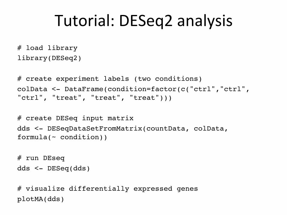
Tutorial: DESeq2 analysis # load librarylibrary(DESeq2)

# create experiment labels (two conditions)colData <- DataFrame(condition=factor(c("ctrl","ctrl", "ctrl", "treat", "treat", "treat")))

# create DESeq input matrix dds <- DESeqDataSetFromMatrix(countData, colData, formula(~ condition))

# run DEseqdds <- DESeq(dds)

# visualize differentially expressed genesplotMA(dds)

# get differentially expressed genesres <- results(dds)

# order by BH adjusted p-valueresOrdered <- res[order(res$padj),]

# top of ordered matrixhead(resOrdered)

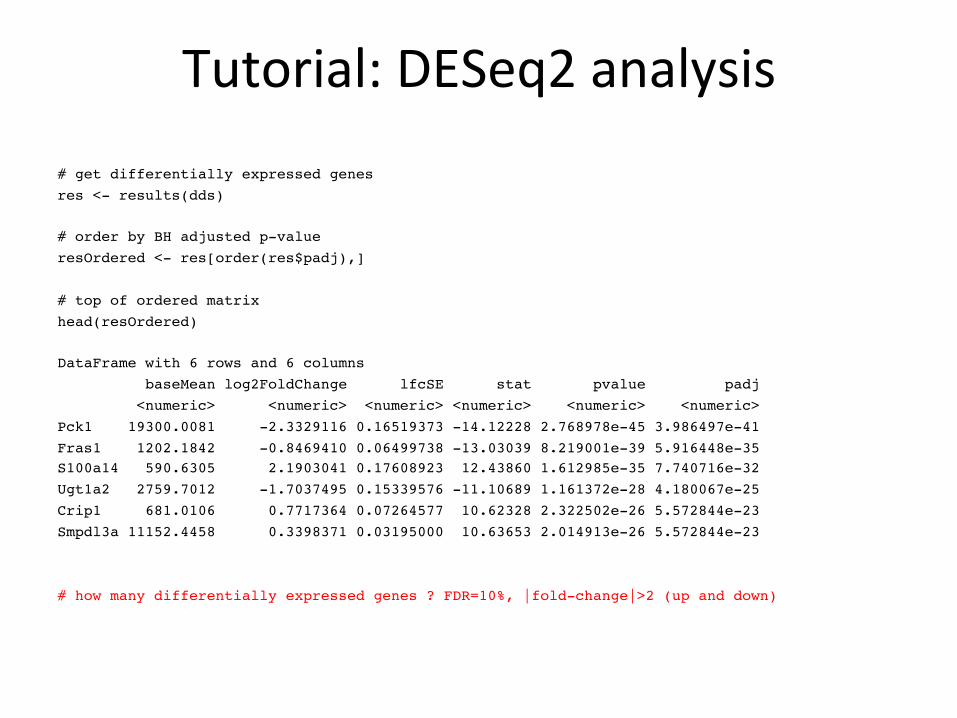
Tutorial: DESeq2 analysis # get differentially expressed genesres <- results(dds)

# order by BH adjusted p-valueresOrdered <- res[order(res$padj),]

# top of ordered matrixhead(resOrdered)

DataFrame with 6 rows and 6 columns baseMean log2FoldChange lfcSE stat pvalue padj <numeric> <numeric> <numeric> <numeric> <numeric> <numeric>Pck1 19300.0081 -2.3329116 0.16519373 -14.12228 2.768978e-45 3.986497e-41Fras1 1202.1842 -0.8469410 0.06499738 -13.03039 8.219001e-39 5.916448e-35S100a14 590.6305 2.1903041 0.17608923 12.43860 1.612985e-35 7.740716e-32Ugt1a2 2759.7012 -1.7037495 0.15339576 -11.10689 1.161372e-28 4.180067e-25Crip1 681.0106 0.7717364 0.07264577 10.62328 2.322502e-26 5.572844e-23Smpdl3a 11152.4458 0.3398371 0.03195000 10.63653 2.014913e-26 5.572844e-23

# how many differentially expressed genes ? FDR=10%, |fold-change|>2 (up and down)

Tutorial: DESeq2 analysis


# get differentially expressed gene matrixsig <- resOrdered[!is.na(resOrdered$padj) &

resOrdered$padj<0.10 & abs(resOrdered$log2FoldChange)>=1,]

Tutorial: DESeq2 analysis


# get differentially expressed gene matrixsig <- resOrdered[!is.na(resOrdered$padj) &

resOrdered$padj<0.10 & abs(resOrdered$log2FoldChange)>=1,]

head(sig)DataFrame with 6 rows and 6 columns baseMean log2FoldChange lfcSE stat pvalue padj <numeric> <numeric> <numeric> <numeric> <numeric> <numeric>Pck1 19300 -2.33 0.165 -14.12 2.77e-45 3.99e-41S100a14 591 2.19 0.176 12.44 1.61e-35 7.74e-32Ugt1a2 2760 -1.70 0.153 -11.11 1.16e-28 4.18e-25Pklr 787 -1.00 0.097 -10.34 4.62e-25 9.49e-22Mlph 1321 1.20 0.117 10.20 1.90e-24 3.42e-21Ifit1 285 1.39 0.156 8.94 3.76e-19 3.38e-16

dim(sig)

# how to create a heat map

Tutorial: Heat Map # how to create a heat map

# select genesselected <- rownames(sig);selected

## load libraries for the heat maplibrary("RColorBrewer")

source("http://bioconductor.org/biocLite.R")biocLite(”gplots”)

library("gplots")

# colors of the heat map

hmcol <- colorRampPalette(brewer.pal(9, "GnBu"))(100) ## hmcol <- heat.colors

heatmap.2( log2(counts(dds,normalized=TRUE)[rownames(dds) %in% selected,]), col = hmcol, scale="row”,

Rowv = TRUE, Colv = FALSE, dendrogram="row", trace="none", margin=c(4,6), cexRow=0.5, cexCol=1, keysize=1 )

Tutorial: Heat Map # how to create a heat maplibrary("RColorBrewer")library("gplots")

# colors of the heat maphmcol <- colorRampPalette(brewer.pal(9, "GnBu"))(100) ## hmcol <- heat.colors

heatmap.2(log2(counts(dds,normalized=TRUE)[rownames(dds) %in% selected,]), col = hmcol, Rowv = TRUE, Colv = FALSE, scale="row", dendrogram="row", trace="none", margin=c(4,6), cexRow=0.5, cexCol=1, keysize=1 )

SelecCng the most differenCally expressed genes and run GO analysis

# universeuniverse <- rownames(resOrdered)

# load mouse annotation and ID librarybiocLite(“org.Mm.eg.db”)library(org.Mm.eg.db)

# convert gene names to Entrez IDgenemap <- select(org.Mm.eg.db, selected, "ENTREZID", "SYMBOL")univmap <- select(org.Mm.eg.db, universe, "ENTREZID", "SYMBOL")

# load GO scoring packagebiocLite(“GOstats”) library(GOstats)

# set up analysisparam<- new ("GOHyperGParams", geneIds = genemap, universeGeneIds=univmap, annotation="org.Mm.eg.db", ontology="BP",pvalueCutoff=0.01, conditional=FALSE, testDirection="over")

# run analysishyp<-hyperGTest(param)

# visualizesummary(hyp)

## Select/sort on Pvalue, Count, etc.

Summary

•  Intro of RNA-‐seq •  EsCmaCng expression levels •  DifferenCal expression analysis with DESeq2

•  Andrea Sboner: [email protected]

rna$seq(dataanalysis(tutorial(physiology.med.cornell.edu/.../2015/...sboner.pdf ·...

Documents