risk premia in the repo market - new york university

Risk Premia in the Repo Market

Josephine Smith∗

November 2012

Abstract

This papers studies movements in short-term repurchase agreement (repo) interestrates. The term structure of U.S. Treasury, agency, and mortgage-backed securityrepos are analyzed from 1997-2012, and the general factor representation is commonacross all of the markets. We also analyze the term structure of spreads between U.S.Treasury and mortgage-backed security repo rates and find unique dynamics, as thesespreads are capturing a term structure of relative collateral risk. When we turn to theissue of risk premia, we find that excess holding period returns are predictable withR2’s higher than 0.2. Additionally, looking at excess holding period returns in thespread market, we find that while the term structure factors do provide some predic-tive power, other measures of macroeconomic and financial stress provide additionalpredictive power. This result provides insight into the type(s) of risk premia beingcaptured in this short-term credit market.

Keywords: Credit spreads; repurchase agreement; risk premia; term structure

∗PRELIMINARY AND INCOMPLETE. Correspondence: Stern School of Business, New York Univer-sity, 44 West 4th Street, Suite 9-86, New York, NY 10012. Email: [email protected]. Phone: (212)998-0171. I’d like to thank my colleagues at NYU Stern for the input, as well as seminar participants atStanford University and Tsinghua University.

1

1 Introduction

Studying the time variaton in risk premia of the term structure of interest rates is a research

area that has been fruitful for decades. Two of the seminal papers in this line include

Fama and Bliss (1987) and Campbell and Shiller (1991), which provided some of the first

empirical documentation of the failure of the expectations hypothesis via forecasting excess

returns. However, much of the research has been focused on U.S. Treasury securities at

maturities of longer than one year for a variety of reasons. First and foremost there are data

limitations, since the U.S. government does not issue extremely short-term debt (i.e. less

than a month). Another reason has been the economic importance of long-term interest

rates, as macro-financial economists have stressed that these interest rates are crucial for

understanding firm investment. While monetary policy is aimed at the short end of the

yield curve (overnight), the idea has always been that movements on the short end can, in

normal times, provide corresponding, desired movements for longer-term rates.

The question of whether time-variation in risk premia, or better yet time-variation in

excess returns, for long-term U.S. Treausry rates exists and if it is predictable has been

asked time and time again. A major contribution to this literature is Cochrane and Piazzesi

(2005), which looks at rates of bonds with maturities between one and five years and finds

that a single, tent-shaped factor constructed from forward rates can predict time-variation

of excess returns with an R2 as high as 0.4. This finding was monumental, since standard

predictability regressions that often used factors of the term structure as predictive variables

failed to generate significant R2’s. Furthermore, these other papers relied on a theoretical

framework of a stochastic discount factor that is capable of pricing all of these factors. The

single factor was novel, but further work by Cochrane and Piazessi (2008) has shown that,

indeed, these term structure factors provide explanatory power above and beyond a single

2

factor for prediction of excess returns on longer-term Treasuries.1

The contribution of this paper is three-fold. First, we study the term structure properties

of short-term repurchase agreement (repo) markets. Repurchase agreements, while com-

plicated in the exact nature of how each market operates and the participants, are at the core

just collateralized loans. The maturity structure we analyze runs from overnight to three-

months. Financial institutions are known to finance their credit using the short end of the

yield curve and lend at the long end, so studying these very short-term lending markets is

interesting from that perspective. We analyze three separate repo markets based on the type

of underlying collateral: U.S. Treasuries, agency securities, and mortgage-backed securi-

ties. Figures (1) and (2) plot the repo rates for each particular type of collateral from 1997

and 2012 at the overnight and three-month maturity, respectively. Until the recent financial

crisis, these repo rates moved nearly one-for-one with the Federal Funds rate. However,

during the crisis, repos with mortgage-backed securities as collateral saw a spike in bor-

rowing rates, being driven by the (potentially mis-priced) risk of the underlying collateral.

We will address this when we study the term structure of repo spreads between rates of

mortgage-backed security and U.S. Treasury repos.

Our next contribution is to document the factor structure of these repo markets. Using

a standard principal component analysis, we show that these short-term repo markets share

a very common underlying factor structure, with the standard level, slope, and curvature

factors prevailing as they do in the more traditional bond market studies. However, the

shape of the factor loadings differ slightly from their more long-term bond market coun-

terparts. In addition, we analyze the factor structure of the term structure of repo spreads

(using mortgage-backed security less U.S. Treasury repo rates), and show that while this

factor structure still contains its own level, slope, and curvature components, the shape

1The breadth of research in this area is enormous. Other work focusing on predictability of bond excessreturns with methodologies similar to this paper include Stambaugh (1988), Kim and Wright (2005), Kimand Orphanides (2005), and Smith (2012).

3

of the factor loadings associated with these is different, leading to contrasting economic

interpretations.

Lastly, we assess the predictability of excess returns in repo markets. We begin by dis-

cussing the definition of excess returns in these markets, since the construction relies on a

strategy of rolling over short-term debt. As a starting point for our predictability regres-

sions, we use the simple term structure factors as our predictive variables. At the quarterly

investment horizon, we find R2’s as high as 0.27. When we analyze predictability of ex-

cess returns of spreads between mortgage-backed security and U.S. Treasury repo rates, we

find that using just the repo term structure factors does not provide much predictive power.

However, this result does not shock us, since we interpret this spread term structure as

fundamentally different from the simple repo term structures as it is reflecting relative risk

across markets. Because of this, we feel as if other variables that reflect macroeconomic

and/or financial risk might provide predictability power for this spread term structure. Us-

ing the VIX as a proxy for financial risk and the Bloom et. al. (2012) policy uncertainty

index as a proxy for macroeconomic risk, we see an increase in R2’s by a factor of four for

the spread term structure. This helps to confirm our hypothesis that, indeed, these spreads

are capturing relative risks, but we do find that it is a combination of macroeconomic and

financial risks. One paper that has addressed short-term bond markets and risk premia with

uncertainty is Mueller, Vedolin, and Zhu (2011), albeit looking at long-term bonds over

short-term investment horizons.

The structure of the paper is as follows. Section 2 describes the data used in the anal-

ysis and the general structure of repurchase agreement markets. Section 3 documents the

factor analysis of each repo market. Section 4 analyzes our excess return predictability

regressions. Section 5 extends the excess return analysis to macroeconomic and financial

risk. Section 6 concludes.

4

2 Description of the Data

Before diving into the analysis of the repo market and its potential risks, it will be of service

to describe the data used in this paper. Three different repo markets will be analyzed:

U.S. Treasury repos, agency repos, and mortgage-backed security repos. These three repo

markets differ in the type of collateral used for the loan. Since the financial crisis, the

literature on repo markets has exploded. Some work on repo markets and risk in the repo

market via haircuts, particularly during the financial crisis, includes Gorton and Metrick

(2012), Jurek and Stafford (2010), and Krishnamurthy, Nagel, and Orlov (2012). We do

not analyze haircuts in this analysis as we are using aggregate repo data, so please reference

these papers for a discussion of haircut volatility during the crisis. We look at overnight,

one-week, two-week, three-week, one-month, two-month, and three-month maturities.2

U.S. Treasury repos are the safest form of repo transaction. The borrower must post

collateral in the form of a pre-specified U.S. Treasury security. Given the low credit risk

of the U.S. government, this type of repo is thought of as safe, and lenders require small

haircuts and charge lower interest rates to borrow in this market. Since we don’t have

U.S. Treasury securities at a maturity of less than one-month, repo rates have provided

practitioners with a measure of short-term, relatively riskless borrowing rates in U.S. fixed

income markets.

Agency repos are considered a slightly less safe form of major repo transactions. The

collateral posted in this transaction takes the form of Federal agency and government-

sponsored enterprise (e.g. Fannie Mae and Freddie Mac) securities. Given the potential

risks underlying these institutions, agency repos are considered slightly less safe compared

to U.S. Treasury repos. However, the recent backing of these institutions via the federal

government has driven some to the opinion that these repos are now much safer, though

2Over 50% of repo transaction occur are overnight repos, though often they remain as open repos and arerolled over.

5

this issue remains a hot topic for discussion.

We also consider mortgage-backed security repos. The collateral underlying these repos

takes the form of high-grade mortgage-backed securities and related derivatives. Since

their inception, these repos have traded at noticeably higher rates than their U.S. Treasury

counterparts given the inherent default risks of the underlying mortgages. However, the

crisis saw a wave of value losses in the underlying collateral of these repos, and the market

seized for quite a bit of time, even though they were ex-ante rated with high credit ratings.

Even now, the current mortgage-backed repo market is noticeably smaller as a fraction of

overall repos.3

Figure (3) plots the breakdown of the repo market as a function of all types of collat-

eral as of July 2012. The data is provided by the Tri-Party Repo Infrastructure Reform

Task Force at the Federal Reserve Bank of New York. The collateral value of the market

totaled nearly $1.8 trillion dollars at the time of the latest data release. As you can see,

U.S. Treasury securities make up a large piece of the repo market, but Agency MBS have

begun to take a larger role in the market since the Federal Reserve began accepting these

as collateral. At the peak of the repo market, nearly $4 trillion dollars of collateral were

outstanding in repos.

Another repurchase agreement we use as a measure of a risk-free repo rate for part

of our analysis is the U.S. Treasury general collateral repo rate. This repo is similar the

U.S. Treasury repo rate, with the exception being that any form of general U.S. Treasury

collateral is accepted. Duffie (1996) formalizes how these repo contracts control for the

specialness that some issues of U.S. Treasuries might face that affects the value of the

underlying collateral, and thus the repo rate itself. We use the overnight general collateral

repo rate when calculating our daily excess returns. For other maturities, we use one-month,

3See the previously-mentioned literature on repo markets for a more detailed analysis on this phenomenon.

6

three-month, and one-year U.S. Treasury strips calculated from Bloomberg.4

3 Factor Analysis of the Repo Term Structure

As a starting point for the empirics, it is useful to perform a standard principal component

analysis on each of the three term structures of repos with varying collateral that were

discussed previously. Models of the term structure in finance often aim to break down

the movements of all yields into a small number of factors. The most common factors

include level, slope, and curvature.5 While the pure finance literature links these factors to

their implied movements in the yield curve, modern macro-finance literature has aimed to

link these factors to macro-financial variables. As an example, Ang and PIazzesi (2003)

found the relationship of similar factors to inflation, output, and monetary policy rates

using an affine model developed theoretically in Duffie and Singleton (1999).6 However,

that analysis was done on the longer-term U.S. Treasury yield curve at a lower frequency

of data collection. Here, our goal is simply to identify these factors at the short end of the

repo yield curve using daily data. In the end, this analysis will prove fruitful when we move

to the analysis of repo spread term structures, as well as using the estimated behavior to

understanding general risk premia in short-term repo markets.

3.1 Repo Term Structure Factor Loadings

Figure (4) plots how a U.S. Treasury repo with maturity from overnight to three-months

loads onto each of the level, slope, and curvature factors. It is here we see where the name

4All data is available from the author upon request. Except for the repo statistics reported in Figure(3), all available data was collected from Bloomberg. To collect the tri-party repo statistics, please visithttp://www.newyorkfed.org/tripartyrepo/.

5The factor analysis was done with more factors, and we will be using the fourth factor in regressionslater in the paper.

6Other work linking the term structure to macroeconomics includes Ang, Dong, and Piazzesi (2007),Gallmeyer et. al. (2007), Rudebusch and Swanson (2008), and Smith and Taylor (2009).

7

of each factor is derived, as is common in the fixed income literature. Each repo loads with

a magnitude of approximately 0.4 on the level factor. Turning to the slope factor, Figures

(5) to (6) plot the factor loadings of the agency and mortgage-backed security repo markets,

respectively, from the estimation using the full time series of data. At first glance, it should

be obvious that yields in all three markets load onto the level, slope, and curvature factors

with similar magnitudes. The loading on the level factor is around 0.4 across all maturities

and markets, as evidenced by the solid line in each figure. The slope factor loadings are

upward-sloping, and the curvature factor loadings have a hump shape. The shapes of these

loadings are also in line with the previous literature on longer-term bond markets, as in

Cochrane and Piazzesi (2005) and (2008), with the exception being that the slope factor

loads onto each maturity in a decreasing fashion. Therefore, increases in the slope factor

in each of these markets is associated with a flattening (or inversion) of the yield curve for

these repos.7 The main takeaway is that these factor loadings are nearly identical in shape

and magnitude across markets, with slight differences in how the curvature factor loading

peaks (at one-week or two-week maturity).

3.2 Spread Term Structure Factor Loadings

Now we move to the factor structure of the mortgage-backed security repo minus U.S. Trea-

sury repo term structure. At each maturity, we compute the spread between the repo rate on

the mortgage-backed security repo and the repo rate on the U.S. Treasury repo. Figure (7)

plots the spreads themselves at the overnight, one-month, and three-month maturities. As

evidenced by the picture, these spreads have not always been zero. There was volatility in

7The correlation of the level factor with other measures of general interest rate movements (i.e. the FederalFunds rate, short-term Treasury rates) is over 0.9 in all cases. As expected, this level factor is capturing theup-and-down movements of all yields in the term structure. Similarly, the slope and curvature factors (barringthe sign of the slope) are capturing the similar movements as their counterparts in the longer-term Treasurymarket, albeit with a slight change in interpretation for the slope factor given the short-term maturities westudy here.

8

the late 1990s, in 2005, and during the recent financial crisis. The spreads have decreased

since the end of the worst part of the crisis. Given that the only difference between these re-

pos is the underlying collateral, the spread is most likely being driven by fundamental risk

differences in the underlying collateral. It is not a surprise that mortgage-backed securities

carry much more credit risk than U.S. Treasuries, and there may also be subtle liquidity

differences across the markets, as well. Regardless of where the risk is coming from, we

see the spread between these repo rates as a measure of financial risk in the repo market.8

It is not common to see a factor analysis performed on a spread term structure, so it

is useful to describe what the factors in this framework are capturing. Figure (8) plots the

first three principal components of this spread term structure, and Figure (9) plots how the

spreads with maturity from overnight to three-months load onto each of the level, slope, and

curvature factors. We call them level, slope, curvature for a reason: they share a similar

shape to the factor loadings we have observed previously. The first factor loads at the same

magnitude across maturities, the second factor loads in a monotonic fashion with maturity,

and the third factor loads in a curved shape across maturities.

What is interesting is to think about the interpretation of these factors. We know that

the level factor of both the mortgage-backed security and U.S. Treasury repos are highly

correlated; they each have a correlation of 0.99 with the Federal Funds rate. However, the

level factor of the spreads has a correlation of 0.09 with the Federal Funds rate. Therefore,

the level factor here is not meant to capture the general level of interest rates, but rather the

general level risk in these repo markets. As discussed above, this relative risk is predomi-

nantly capturing the differential risk in the underlying collateral. An increase in this level

risk causes spreads to increase at the same magnitude across all maturities.

The slope and curvature factors remain a bit of a mystery in terms of their economic

8We could also look at the difference between agency and U.S. Treasury repo markets, and the appendixprovides results for this analysis.

9

interpretation. An increase in the slope factor causes the shortest-term rates to fall and the

longer-term rates to rise, in contrast to the slope factor for each of the individual repos mak-

ing up the spread. This is an interesting phenomenon. While an increase in the slope factor

of each of the mortgage-backed security and U.S. Treasury repos causes their individual

yield curves to flatten (or invert), an increase in the slope factor of their spread causes its

yield curve to become more upward-sloping. While a flattening of the yield curve for the

level of interest rates can often signal worsening economic conditions, it is of interest that

more study be done on the flattening of the yield curve for spreads, since it is not nec-

essarily capturing the flattening of the yield curve of the individual securities making up

the spread. Turning to the curvature factor, we again see a shift in the shape relative to

the mortgage-backed security and U.S. Treasury repo factor loadings, which each had a

hump shape. Here, the factor loadings for the curvature factor of the spreads is u-shaped.

Increases in the curvature factor cause the shortest- and longest-term interest rates to rise

and those in-between to fall.

To summarize, the factor loadings for the spread term structure have stark contrasts to

the factor loadings of both of the mortgage-backed security and U.S. Treasury repos. There

is a large open question as to what these spread factors represent, but in general they are

capturing movements in relative collateral risk across the two markets.

4 Excess Return Predictability

Before barraging the reader with excess return regressions, it is important to understand

how excess returns are calculated in this framework. To do this, let us solidify some general

notation. Though repos don’t function exactly like zero-coupon bonds, we can borrow the

notation since we are simply just formalizing theory for a shorter-term collateralized loan

contract with no intermediate interest payments.

10

4.1 Excess Return Notation and Theory

Let p(n)t denote the log price of a n-period discount bond at time t. The continuously-

compounded yield of this n-period discount bond is therefore

i(n)t =−n−1 p(n)t . (1)

It is important to keep track of n and t throughout the analysis. t represents the time sample,

which is daily. n, on the other hand, represents the maturity of the repo, which ranges from

overnight to three months.

Let’s begin with a situation where we purchase a n-period bond (i.e. lend money) at

time t and sell it one period later at time t +1 when it is now a n−1 period bond. The log

holding period return from this strategy is given by

r(n)t+1 = p(n−1)t+1 − p(n)t (2)

= ni(n)t − (n−1)i(n−1)t+1 . (3)

We denote the excess log holding period return as

rx(n)t+1 = r(n)t+1 − i(1)t , (4)

where i(1)t is the market risk-free return over the holding period.9 From the expectations

hypothesis, any time variation in this excess log holding period return is capturing time-

varying risk premia, and the goal of this section is to understand if it is predictable.

This analysis is appropriate when we are looking at bonds whose maturity is longer than

the investment horizon (holding period). What about when bonds mature before the end of

9Admittedly, this notation ignores approximation results from using logs, but we will rely on conveniencefor this framework.

11

the investment horizon? For this, we must determine how to calculate excess log holding

period returns from rolling over short-term debt. For the sake of an example, suppose our

investment horizon is n. There are two ways of getting money from time t to time t + n:

either invest in the n-period bond, or roll over one-period bonds until the n− 1-maturity

bond matures. The expectations hypothesis states that the return from these two strategies

must be the same, namely that:

i(n)t =1nEt[i(1)t + i(1)t+1 + · · ·+ i(1)t+n−1

]. (5)

If this equation does not hold, then the expectations hypothesis is violated, and any time

variation in the difference is capturing time-varying risk premia. The log holding period

return is being captured by the right-hand side of equation (5), and thus the excess log

holding period return is captured by the difference of the righthand side and lefthand side

of equation (5).

While it may not seem obvious, equation (2) and (4) are capturing the same excess hold-

ing period return. However, it is important to remember how it is calculated, and to note

that studying the behavior of time-varying risk premia via equation (5) is not commonplace

in the literature since risk premia are not studied in such short-term markets frequently.10

We find it important to understand if risk premia are indeed predictable when calculated

in this way, since we are now capturing the risk of rolling over short-term debt (one of the

main uses of the repo market).

10An exception to this is the work of Smith (2012), who studies risk premia in the LIBOR-OIS termstructure and finds evidence of predictable time variation in risk premia at a weekly investment horizon.

12

4.2 Are Excess Returns Predictable?

With the yield curve factors in hand for each repo market, the next logical question is

whether or not these factors can predict time-varying risk premia in these markets. There

are two immediate concerns with this. First, the markets we are analyzing have a maximum

maturity of three months, truly capturing the short end of the yield curve. Most of the

previous work on fixed income risk premia looks at longer-term bonds, and it is sometimes

difficult to predict time variation in risk premia in these markets. One obvious exception to

this observation is Cochrane and Piazessi (2005), who identify a single tent-shaped factor

comprised of forward rates that explains up to 44% of the variation in risk premia. However,

we are trying to assess whether or not time-varying risk premia exist in these short-term

markets and if, indeed, they are predictable.

A second issue is that fact that, conditional on the existence of time-varying risk premia

in bond markets, it is not often the case that standard yield curve factors like level, slope,

and curvature provide much predictive power. Intuitively, general movements in yields

(captured by the factors) are not necessarily correlated with general movements in risk pre-

mia. This intuition is not new, but the results below will show that the previously published

magnitude of predictive power of yield curve factors using longer-term bond yields differs

when we looks at short-term yields from the repo market.

For the U.S. Treasury, agency, and mortgage-backed security repos, excess holding pe-

riod returns are calculated using daily data at the daily, quarterly, and annual frequency.11

While repos are not standard bonds, there is a natural interpretation of each of these re-

turns. The holding period return at the daily frequency captures the return captured from

unwinding a repo position after one day. It is more interesting to look at the holding pe-

11SInce we do not have repos at each continuous maturity, we use the Campbell-Shiller approximation:

aprx(n)t+1 = ni(n)t −ni(n)t+1 − i(1)t . (6)

13

riod returns at the quarterly and annual frequencies. For example, let’s use the one-month

repo as our maturity of interest. What does it mean if we hold a one-month repo for one

quarter? This holding period return is constructed to be the same as the return from rolling

over a one-month repo each month for one quarter. Similarly, the annual holding period

return of a one-month repo is constructed to be the same as the return from rolling over a

one-month repo each month for one year. To construct excess returns, we must substract

from the holding period return a measure of the riskless rate for that given return horizon.

For the daily frequency, we use the overnight general collateral repo rate. For the quarterly

frequency, we use the three-month U.S. Treasury strip. Lastly, for the annual frequency, we

use the one-year U.S. Treasury strip.

The baseline regression of excess returns for maturity n on factors for the corresponding

market will be of the form

aprx(n)t+1 = α(n)+β (n)1 PCt(1)+β (n)

2 PCt(2)+β (n)3 PCt(3)+β (n)

4 PC(4)+ ε(n)t+1, (7)

where PC(1), PC(2), PC(3), and PC(4) are the first four principal components of the term

structure in each of the three repo markets. We will run this regression for each maturity n

in each individual repo market. Later, we will ask the question of whether other financial

variables have predictive power.

4.2.1 U.S. Treasury Repos

Table (2) displays the coefficients[β (n)

1 β (n)2 β (n)

3 β (n)4

]as a function of the maturity for the

U.S. Treasury repo. Panel A captures the coefficients for daily returns, Panel B captures the

coefficients for quarterly returns, and Panel C captures the coefficients for annual returns.

Under each coefficient estimate, we provide standard errors computed using a Newey-West

adjustment with 18 lags. To begin with Panel A, we can see that daily returns are high

14

predictable using just the first four principal components of the U.S. Treasury repo term

structure. The R2’s are falling with maturity with these daily excess returns, which is not

surprising. The magnitude of the R2’s is promising, particularly for the one-, two-, and

three-month repo daily excess returns.

Moving onto the quarterly returns, this will be the reader’s first glimpse into excess

return predictability when looking at a rollover holding period return strategy. For the sake

of exposition, we abbreviate the results and display only the predictability results for the

overnight, one-week, and one-month repos. There is strong predictive power for each type

of repo over a quarterly return horizon with R2’s of approximately 0.2. Finally, with the

annual returns, we still have noticeable predictability, with R2’s as high as 0.18 for the

one-month repo. This implies that if one were to roll over one-month repos for a year and

compare the return of that strategy to holding just a one-year bond, then 18% of the time-

variation in that excess return is captured by the first four principal components of the repo

term structure. While some of these R2’s may not be of the magnitude of those in Cochrane

and Piazzesi (2005), we are looking at a much shorter-term market and rollover returns

comparisons, and we believe these results are strong.

Looking at the coefficients themselves, we see that for each investment horizon, all

maturities are loading on the first principal component with similar magnitude, though this

factor does not carry much explanatory power for the annual returns in Panel C. For daily

returns, this factor loads with a coefficient of around -0.4, while with quarterly returns the

loading hovers around 0.9. Interestingly, the statistical significance of the term structure

factors varies depending on the investment horizon. The third and fourth principal com-

ponents are statistically significant for daily returns at various horizons (above and beyond

that provided by the first principal component). For quarterly returns, the first two princi-

pal components provide statistically significant coefficients and predictive power. Lastly,

for annual returns, we see that the second and third principal components are statistically

15

significant, and the first principal component does not provide much predictive power for

these regressions.

4.2.2 Agency Repos


1 β (n)2 β (n)

3 β (n)4

]as a function of the maturity for

the agency repo market. Panel A captures the coefficients for daily returns, Panel B cap-

tures the coefficients for quarterly returns, and Panel C captures the coefficients for annual

returns. Under each coefficient estimate, we provide standard errors computed using a

Newey-West adjustment with 18 lags. Starting again with daily returns, we see continued

predictive power of the agency repo term structure factors, in line with those we saw for

U.S. Treasury repos (though marginally lower at the three-month maturity). The magnitude

of the coefficients is even the same across the U.S. Treasury and agency repo markets. At

the quarterly return horizon, we have R2’s hovering around 0.23, and most of the action

is coming from the first principal component. For annual returns, the predictive power

drops, but interestingly the second and third principal components are again the drivers of

predictive movements in excess returns.

4.2.3 Mortgage-Backed Security Repos


1 β (n)2 β (n)

3 β (n)4

]as a function of the maturity for the

mortgage-backed security repo market. Panel A captures the coefficients for daily returns,

Panel B captures the coefficients for quarterly returns, and Panel C captures the coefficients

for annual returns. Under each coefficient estimate, we provide standard errors computed

using a Newey-West adjustment with 18 lags. In the end, much of the same predictabil-

ity results remain as for U.S. Treasury and agency repos, with slightly better predictive

performance at the quarterly return horizon.

To sum up these excess returns regressions, we have found significant predictive power

16

of the principal components in each repo market for the excess returns in that repo market at

the daily, quarterly, and annual investment horizon. At the daily return horizon, predictabil-

ity is decreasing in maturity of the underlying repo. For the quarterly and annual horizons,

however, the predictability content is rather stable. Recall that these last two investment

horizons were taking account of the fact that the excess returns were from a rolling over

strategy of short-term debt for the length of the investment horizon.

4.3 Excess Return Predictability for Repo Spreads

We now turn to the term structure of spreads between mortgage-backed security repo rates

and U.S. Treasury repo rates. In an effort to assess whether excess returns are predictable,

we choose to link this term structure of spreads to the term structure of our safest type of

repo, the U.S. Treasury repo.12 To begin, it is important to understand what we mean by an

excess returns on a strategy involving investment in an interest rate spread. While this trade

is not as natural in interpretation as for a long-term bond, the way in which excess returns

are computed is identical. For spread maturities longer than the investment horizon, the

holding period return is derived from holding a portfolio of the spread between mortgage-

backed security repos and U.S. Treasury repos for a given maturity and then selling it at the

end of the investment horizon. For spread maturities shorter than the investment horizon,

the holding period return is derived from rolling over a portfolio of the spread between

mortgage-backed security repos and U.S. Treasury repos. We compare these holding period

returns from the return one would derive from holding the spread with a maturity equal to

the investment horizon.


1 β (n)2 β (n)

3 β (n)4


spreads between mortgage-backed security and U.S. Treasury repo rates, and the predictive

12Interestingly, there is very little predictability derived from the principal components of the spread termstructure itself, which provides a new set of questions for future research.

17

variables are the first four principal components of the U.S. Treasury repo term structure

used in Table (2). Panel A captures the coefficients for daily returns, Panel B captures the

coefficients for weekly returns, and Panel C captures the coefficients for quarterly returns.13


adjustment with 18 lags. The R2’s for these regressions are substantially lower than those

for the level term structures, with a peak of 0.11 for the daily excess return on one-month

repo. However, moving to the quarterly investment horizon sees the R2’s cut in half. While

these results are not as exciting as the previous predictability results, we will discuss in

more detail the interpretation of excess returns in this market in the next section and show

that other macro-financial indices provide more predictive power.

4.4 Sharpe Ratios of the Repo Term Structure

An interesting statistic commonly used to understand average risk premia in bond markets

is the Sharpe ratio. The Sharpe ratio in this environment is going to capture constant risk

premia, or risk premia on average over the sample period addressed. The formula for

computing the Sharpe ratio is given by:

SR(n) =E[arx(n)t+1]

σ [arx(n)t+1], (8)

i.e., it is the mean of the excess return divided by its standard deviation. Sharpe ratios are

most commonly used in portfolio optimization analysis to determine how one can maxi-

mize portfolio performance via the mean-variance frontier. A standard benchmark is that

the market stock portfolio has a Sharpe ratio of approximately 0.5.

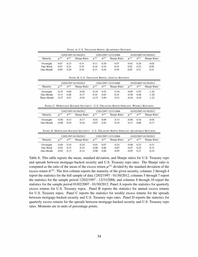
Table (6) provdes a breakdown of Sharpe ratios using excess returns of both the U.S.

13We only go out to the quarterly return horizon since we want to benchmark to the quarterly spread as thecomparable security.

18

Treasury repos and the spread between mortgage-backed security and U.S. Treasury re-

pos. We also compute the Sharpe ratios over different subsamples to provide the reader a

glimpse into how Sharpe ratios might have changed after the start of the recent financial

crisis. Panel A looks at Sharpe ratios computed from quarterly returns of U.S. Treasury

repos, while Panel B looks at annual returns of U.S. Treasury repos. The first column is the

maturity of the underlying repo. Columns 2 through 4 provide the mean µ(n) of the excess

returns, the standard deviation σ (n) of the excess returns, and the Sharpe ratio for the entire

sample period. Columns 5 through 7 do the same, but just for the period of 12/01/1997-

12/31/2006. The last three columns focus on the period that includes the financial crisis,

and thus this period starts on 01/02/2007 and ends at the end of our full sample.

Starting with Panel A at the quarterly investment horizon, we see that Sharpe ratios are

small, particularly during the crisis period. In fact, there is a surprising drop in the level of

the Sharpe ratio during the financial crisis, being driven by the fact that both the mean of

the excess returns fell while the volatility of the excess returns rose. Turning to Panel B at

the annual investment horizon, we see a shift in both the sign and magnitude of the Sharpe

ratios. Almost all of the Sharpe ratios are negative, and during the crisis they are largely

negative, on the order -1.25. This is not particulary surprising to us, since we are assessing

a very risky strategy of rolling over short-term debt for a year. Particularly during the crisis,

we might expect that the risk of such a strategy is further exacerbated by the high volatility

of interest rates during the period.

Panels C and D report the results from a similar analysis for the weekly and quarterly

returns, respectively, of spreads between mortgage-backed security and U.S. Treasury repo

rates. Here, it is important to note that the Sharpe ratios are always negative and small,

mostly driven by the fact that the mean of all of these excess returns is negative and small.

It is important to note that the Sharpe ratios are, again, much higher during the financial

crisis period than before the crisis. However, we provide these Sharpe ratio results as a

19

method for the reader to understand average risk premia in these markets. Note that these

strategies look awful by the investment horizon measures we entertain. Why in the world

would investors ever roll over short-term repo instead of investing in the long-term? That is

a fundamental question for a variety of financial institutions, as they perform this strategy

every single day. One of the easiest ways to answer the question is that they simply don’t

care about mean and variance over these investment horizons, which is the stance that we

also take. Also, these institutions, as discussed previously, can find rolling over short-term

debt as ex-ante less costly if they face enormous credit risk when trying to issue long-term

debt.

5 Macroconomic vs. Financial Risks and Repo Markets

With a barrage of risk premia predictability results, we now turn to the bigger picture of

understanding if there are other macroeconomic or financial measures of risk or uncer-

tainty that provide additional predictive power for excess returns in the repo markets as

well as the spread repo market. Our motivation for this analysis comes from the fact that

macroeconomic and/or financial market uncertainty plays a role in explaining risk premia

in short-term fixed income markets.14

As a laboratory for studying whether macroeconomic or financial risks are predictive

of risk premia in repo markets, we use two different variables to proxy for risk. The first

is an old standard: the S&P VIX. The VIX, or volatility index, is constructed to capture

volatility in the stock market, and is often used as a proxy for uncertainty in the stock

market. Even though it is meant to capture stock market volatility, it is without question

that the fixed income and stock markets are correlated, and we believe that the VIX can

provide particularly informative power for the short-end of the yield curve given its reliance

14That is not to say that it doesn’t also play a role in longer-term fixed income markets. Some papersaddressing this topic include Buraschi and Whelan (2010) and Hsu (2011).

20

on day to day fluctuations in market news and uncertainty.

The second variable we use to proxy for uncertainty is the newly-developed policy

uncertainty index found in Bloom et. al (2012). This index is constructed using three types

of information: newspaper articles covering policy-related economic news, federal tax code

provisions nearing expiration, and dispersion among forecasters regarding policy-related

forecasts. While this index is calculated ex-post, we are using it here to ascertain whether it

has predicted power for future returns over varying investment horizons. Interestingly, this

index is constructed using what the authors believe is purely policy-related macroeconomic

news, and thus it is in contrast to the VIX which is meant to capture high-frequency stock

market volatility.15 Figure (13) plots the movements in these two indices over our sample

period.

We run a set of regressions similar in spirit to (7) with a slight adjustment:

aprx(n)t+1 = α(n)+4

∑i=1

β (n)i PCt(i)+β5PIt +β6V IXt + ε(n)t+1, (9)

where now we have added in both the policy index PI and the VIX V IX as part of the

predictability regression. We will run these regressions in two stages: first, we include just

the policy index, and then we add in both the policy index and the VIX. While these two

indices are correlated (our sample correlation is approximately 0.5), our prior is that they

are capturing fundamentally different types of risk.

15This index has been used in as empirical tests for the importance of policy risk. See Pastor and Veronesi(2012) as an example of such an application.

21

5.1 U.S. Treasury Repo Excess Returns and Uncertainty

Our first set of excess returns regressions looks at the U.S. Treasury repo market.16 Table

(7) displays the coefficients[β (n)

1 β (n)2 · · · β5

]as a function of the maturity for the U.S.

Treasury repo market, where we include just the policy index PI as an additional explana-

tory variable. Panel A captures the coefficients for daily returns, Panel B captures the

coefficients for quarterly returns, and Panel C captures the coefficients for annual returns.


adjustment with 18 lags. The takeaway from this that the policy index does not help in

predictability of excess returns at the daily investment horizon, there is slight improvement

at the quarterly horizon, and there is predictability improvement at the annual investment

horizon. At the annual horizon, R2’s increase by three percentage points for each repo ma-

turity, peaking at an R2 of 0.21 for the one-month maturity repo. While these changes are

not large, we are, to our knowledge, the first to document the potential predictive power of

this new policy index for longer-term excess returns using short-term financial assets.

Turning to our second set of excess returns regressions for the U.S. Treasury repo mar-

ket, Table (8) displays the coefficients[β (n)

1 β (n)2 · · · β5 β6

]as a function of the maturity

for the U.S. Treasury repo market, where we include both the policy index PI and the VIX

V IX as additional explanatory variables. Panel A captures the coefficients for daily returns,

Panel B captures the coefficients for quarterly returns, and Panel C captures the coefficients

for annual returns. Under each coefficient estimate, we provide standard errors computed

using a Newey-West adjustment with 18 lags. Here, we only see slight or no increase in

predictive power for these excess returns. Therefore, while the policy index does provide

some noticeable predictability benefit for U.S. Treasury repos, the VIX is almost insignifi-

cant. Our general interpretation of this results is that movements in the U.S. Treasury repo

16Regression results for the agency and mortgage-backed security repos are available on request. Theresults are robust across these markets, as well.

22

term structure are picking up movements in policy uncertainty, predominantly due to their

close linkage to movements in the Federal Funds rate over time. Risk premia of U.S. Trea-

sury repos, as constructed here, is correlated with some elements of macroeconomic risk.

However, we would not argue that there is not financial risk; it may just be picked up in the

principal components used in the regression.

5.2 Repo Rates Spreads and Macroeconomic vs. Financial Risks

In the previous section, we found that standard factors did not explain excess returns on

spreads between mortgage-backed security and U.S. Treasury repos with meaningful R2’s.

However, given that this spread is a measure of relative collateral risk, and the excess

returns captures risk premia embedded in spreads, it is interesting to analyze whether the

policy uncertainty index or VIX provide any insight into predictability of excess returns.


1 β (n)2 · · · β5 β6


spreads between mortgage-backed security and U.S. Treasury repo rates, where we include

both the policy index PI and the VIX V IX as additional explanatory variables. Panel A

captures the coefficients for daily returns, Panel B captures the coefficients for quarterly

returns, and Panel C captures the coefficients for annual returns. Under each coefficient

estimate, we provide standard errors computed using a Newey-West adjustment with 18

lags. We do two sets of regressions, one with just the policy index and one with both the

policy index and the VIX.

Looking at the first two rows of each panel, which report the results using the policy

index as an additional explanatory variable and comparing to Table (5), we see that the

R2’s do not change at the daily or weekly investment horizons, but there is a dramatic

increase at the quarterly horizon. The R2 doubles from around 0.05 using just the U.S.

Treasury repo principal components to around 0.1 after including the policy index. Even

23

more impressive, when we add in the VIX we see that the R2 doubles yet again, ending

with an R2 of around 0.2. This leads us to two conclusions: first, the VIX carries much

more explanatory power for these excess returns than the policy index, and second that

both variables carry significant power in predicting excess returns over longer investment

horizons. In contrast to the U.S. Treasury repo term structure, we believe that the spread

term structure is picking up both macroeconomic and financial risks, though predominantly

the latter.

6 Conclusion

We study the term structure of short-term repo markets with varying types of collateral

from 1997-2012. We find that the term structure of repos have unique qualities above

and beyond their extremely short maturity. Computing excess holding period returns, we

assess that predictability of these excess returns is possible using standard level, slope,

and curvature factors from the repo markets. As a measure of repo stress, we look at the

term structure of the spread between mortgage-backed security and U.S. Treasury repo

rates. The underlying factor structure of this market differs substantially to that of each

of the underlying repos, mostly due the fact that these spreads are, in and of themselves,

capturing relative risk of the underlying collateral. Using repo factors, as well as measures

of macroeconomic and financial risk, we are able to show meaningful predictability of risk

premia in this spread term structure, as well.

There are a variety of open questions and further avenues of research coming from these

results. An obvious extension is to use a more theoretical framework to model the behavior

these term structures, such as an affine model, in an effort to use no-arbitrage restrictions to

back out time varying risk premia. It is also important to understand exactly which type of

risks we are capturing in these markets. Is the risk macroeconomic, financial, or both? Is

24

there ever a hope of distinguishing between the two? We feel that the identification of short-

term risk premia is crucial for our understanding of the linkages between macroeconomic

and financial risk due to the prevalence of financing activity by major financial institutions

using repo markets and the correlation of these short-term rates with policy rates in the U.S.

and globally.

25

References

ANG, A., S. DONG, AND M. PIAZZESI (2007): “No-Arbitrage Taylor Rules,” Unpublished

Manuscript.

ANG, A., AND M. PIAZZESI (2003): “A No-Arbitrage Vector Autoregression of Term

Structure Dynamics with Macroeconomic and Latent Variables,” Journal of Monetary

Economics, 50(4), 745–787.

BAKER, SCOTT, B. N., AND S. DAVIS (2012): “Measuring Economic Policy Uncertainty,”

Unpublished Manuscript.

BLISS, R. R., AND E. F. FAMA (1987): “The Information in Long-Maturity Forward

Rates,” American Economic Review, 77, 680–692.

BURASCHI, A., AND P. WHELAN (2010): “Macroeconomic Uncertainty, Difference in

Beliefs, and Bond Risk Premia,” CAREFIN Research Paper No. 27/2010.

CAMPBELL, J. Y., AND R. J. SHILLER (1991): “Yield Spreads and Interest Rate Move-

ments: A Bird’s Eye View,” Review of Economic Studies, 58, 495–514.

COCHRANE, J., AND M. PIAZZESI (2008): “Decomposing the Yield Curve,” Unpublished

Manuscript.

COCHRANE, J. H., AND M. PIAZZESI (2005): “Bond Risk Premia,” American Economic

Review, 95(1), 138–160.

DUFFIE, D. (1996): “Special Repo Rates,” Journal of Finance, 51(2), 493–526.

DUFFIE, D., AND K. SINGLETON (1999): “Modeling Term Structures of Defaultable

Bonds,” Review of Financial Studies, 12, 687–720.

26

GALLMEYER, M. F., B. HOLLIFIELD, F. J. PALOMINO, AND S. E. ZIN (2007):

“Arbitrage-Free Bond Pricing with Dynamic Macroeconomic Models,” Federal Reserve

Bank of St. Louis REVIEW, pp. 205–326.

GORTON, G., AND A. METRICK (2012): “Securitized Banking and the Run on Repo,”

Journal of Financial Economics, 104(3), 425–451.

HSU, A. (2011): “Does Fiscal Policy matter for Treasury Bond Risk Premia?,” Unpub-

lished Manuscript.

JUREK, J. W., AND E. STAFFORD (2010): “Crashes and Collateralized Lending,” Unpub-

lished Manuscript.

KIM, D. H., AND A. ORPHANIDES (2005): “Term Structure Estimation with Survey Data

on Interest Rate Forecasts,” Finance and Economics Discussion Series, 2005.

KIM, D. H., AND J. H. WRIGHT (2005): “An Arbitrage-Free Three-Factor Term Struc-

ture Model and the Recent Behavior of Long-Term Yields and Distant-Horizon Forward

Rates,” Finance and Economics Discussion Series, 2005.

KRISHNAMURTHY, A., S. NAGEL, AND D. ORLOV (2012): “Sizing Up Repo,” Unpub-

lished Manuscript.

MUELLER, PHILIPPE, V. A., AND H. ZHU (2011): “Short-Run Bond Risk Premia,” Fi-

nancial Markets Group Discussion Paper 686.

PASTOR, L., AND P. VERONESI (2012): “Political Uncertainty and Risk Premia,” Unpub-

lished Manuscript.

RUDEBUSCH, G., AND E. SWANSON (2008): “Examining the Bond Premium Puzzle with

a DSGE Model,” Journal of Monetary Economics, 55, 111–126.

27

SMITH, J. (2012): “The Term Structure of Money Market Spreads during the Financial

Crisis,” Unpublished Manucript.

SMITH, J., AND J. B. TAYLOR (2009): “The Term Structure of Policy Rules,” Journal of

Monetary Economics, 56, 907–917.

STAMBAUGH, R. F. (1988): “The Information in Forward Rates: Implications for Models

of the Term Structure,” Journal of Financial Economics, 21, 41–70.

28

PANEL A: U.S. TREASURY REPOS

12/02/1997-01/30/2012 01/02/2007-01/30/2012Maturity Mean Standard Deviation Mean Standard Deviation

Overnight 2.79 2.18 1.33 1.91One-Week 2.79 2.16 1.35 1.90Two-Week 2.79 2.16 1.34 1.89

Three-Week 2.79 2.16 1.34 1.88One-Month 2.79 2.16 1.34 1.87Two-Month 2.80 2.16 1.34 1.86

Three-Month 2.81 2.16 1.34 1.86

PANEL B: AGENCY REPOS




Three-Month 2.89 2.16 1.46 1.93

PANEL C: MORTGAGE-BACKED SECURITY REPOS




Three-Month 2.93 2.17 1.53 1.94

Table 1: This table reports the mean and standard devation of each yield comprising the term struc-ture of the U.S. Treasury, agency, and MBS repos. Panel A reports the summary statistics for theU.S. Treasury repo term structure, Panel B reports the summary statistics for the agency repo termstructure, and Panel C reports the summary statistics for the MBS repo term structure. ColumN 1reports the maturity of the repo. Columns 2 and 3 report the mean and standard deviation, respec-tively, of the repos over the full time sample 12/02/1997 - 01/30/2012. Columns 4 and 5 reportthe mean and standard deviation, respectively, of the repos over the late time sample 01/01/2007 -01/30/2012. Units are in percentage points.

29

PANEL A: DAILY RETURNS

Maturity PC(1) PC(2) PC(3) PC(4) R2

One-Week -0.38 -0.33 1.07 -0.29 0.96(0.00) (0.12) (0.30) (0.87)

Two-Week -0.38 -0.25 1.89 -0.39 0.89(0.00) (0.16) (0.45) (1.02)

Three-Week -0.38 -0.30 2.15 -2.36 0.80(0.00) (0.35) (0.52) (1.92)

One-Month -0.37 -0.44 2.84 10.35 0.62(0.00) (0.51) (0.86) (5.57)

Two-Month -0.37 -0.92 3.71 -5.86 0.43(0.00) (0.79) (1.08) (4.01)

Three-Month -0.37 -1.83 2.71 -10.13 0.25(0.01) (0.99) (2.05) (5.80)

PANEL B: QUARTERLY RETURNS


Overnight 0.02 -0.10 -0.23 0.03 0.17(0.00) (0.06) (0.15) (0.10)

One-Week 0.02 -0.10 -0.09 0.04 0.18(0.00) (0.06) (0.15) (0.10)

One-Month 0.02 -0.05 0.15 -0.10 0.23(0.00) (0.05) (0.13) (0.09)

PANEL C: ANNUAL RETURNS


Overnight -0.01 -0.65 -1.80 0.00 0.15(0.01) (0.17) (0.26) (0.31)

One-Month 0.02 -0.82 -2.06 0.09 0.18(0.01) (0.19) (0.30) (0.36)

Three-Month -0.00 -0.55 -1.37 0.02 0.12(0.01) (0.15) (0.23) (0.25)

Table 2: This table displays the results from the regressions aprx(n)t+1 = α(n) +

β (n)1 PCt(1)+β (n)

2 PCt(2) + β (n)3 PCt(3)+β (n)

4 PCt(4) + ε(n)t+1, where aprx(n)t+1 is the approximate

excess holding period return over holding period n at time t + 1 for the given U.S. Treasury repoand PCt(i) is the ith principal component of the U.S. Treasury repo term structure. The first columnis the maturity of the repo, the second through fifth columns display the coefficient estimates, andthe sixth column is the R2 of the regression. Below each coefficient estimate is a standard error witha Newey-West correction with 18 lags. Panel A reports daily excess returns regressions, Panel Breports quarterly excess returns regressions, and Panel C reports annual excess returns regressions.The sample period is daily from 12/02/1997-01/30/2012.

30



One-Week -0.37 -0.14 0.95 -1.36 0.92(0.00) (0.13) (0.29) (0.42)

Two-Week -0.37 0.04 2.52 2.71 0.73(0.00) (0.21) (0.88) (2.05)

Three-Week -0.37 0.06 3.27 4.57 0.56(0.01) (0.27) (1.12) (3.17)

One-Month -0.37 -0.11 2.83 -3.20 0.46(0.01) (0.27) (1.12) (1.82)

Two-Month -0.36 -0.24 2.69 -0.62 0.20(0.01) (0.56) (1.17) (0.73)

Three-Month -0.35 -0.21 2.77 -0.31 0.10(0.02) (0.82) (1.63) (1.12)



Overnight 0.02 0.05 -0.17 -0.14 0.22(0.00) (0.08) (0.10) (0.11)

One-Week 0.02 0.01 -0.08 -0.12 0.23(0.00) (0.07) (0.09) (0.09)

One-Month 0.02 0.02 0.13 0.11 0.24(0.00) (0.07) (0.10) (0.10)



Overnight 0.00 -0.74 -1.29 -0.31 0.11(0.01) (0.23) (0.27) (0.38)

One-Month 0.02 -1.01 -1.56 -0.38 0.16(0.01) (0.25) (0.30) (0.45)

Three-Month 0.00 -0.66 -1.06 -0.31 0.10(0.01) (0.19) (0.23) (0.30)


β (n)1 PCt(1)+β (n)

2 PCt(2) + β (n)3 PCt(3)+β (n)


excess holding period return over holding period n at time t + 1 for the given agency repo andPCt(i) is the ith principal component of the agency repo term structure. The first column is thematurity of the repo, the second through fifth columns display the coefficient estimates, and thesixth column is the R2 of the regression. Below each coefficient estimate is a standard error witha Newey-West correction with 18 lags. Panel A reports daily excess returns regressions, Panel Breports quarterly excess returns regressions, and Panel C reports annual excess returns regressions.The sample period is daily from 12/02/1997-01/30/2012.

31



One-Week -0.37 -0.40 0.66 -1.10 0.97(0.00) (0.14) (0.27) (0.42)

Two-Week -0.37 -0.41 1.64 -0.87 0.93(0.00) (0.20) (0.49) (0.41)

Three-Week -0.37 -0.50 2.12 0.96 0.87(0.00) (0.27) (0.51) (0.65)

One-Month -0.37 -0.68 1.38 5.45 0.80(0.00) (0.30) (0.41) (0.70)

Two-Month -0.37 -1.42 -0.47 4.67 0.42(0.01) (0.66) (1.28) (1.69)

Three-Month -0.37 -2.23 -2.42 -7.63 0.26(0.01) (0.90) (2.29) (4.15)



Overnight 0.02 0.01 -0.17 0.34 0.27(0.00) (0.07) (0.09) (0.17)

One-Week 0.02 -0.07 -0.12 0.33 0.27(0.00) (0.06) (0.09) (0.16)

One-Month 0.02 -0.14 0.09 0.45 0.27(0.00) (0.06) (0.11) (0.20)



Overnight 0.00 -0.32 -1.08 -1.01 0.06(0.01) (0.26) (0.26) (0.59)

One-Month 0.02 -0.51 -1.29 -1.12 0.11(0.01) (0.30) (0.31) (0.66)

Three-Month 0.00 -0.39 -0.88 -0.65 0.07(0.01) (0.19) (0.22) (0.41)


β (n)1 PCt(1)+β (n)

2 PCt(2) + β (n)3 PCt(3)+β (n)


excess holding period return over holding period n at time t + 1 for the given mortgage-backedsecurity repo and PCt(i) is the ith principal component of the mortgage-backed security repo termstructure. The first column is the maturity of the repo, the second through fifth columns displaythe coefficient estimates, and the sixth column is the R2 of the regression. Below each coefficientestimate is a standard error with a Newey-West correction with 18 lags. Panel A reports dailyexcess returns regressions, Panel B reports quarterly excess returns regressions, and Panel C reportsannual excess returns regressions. The sample period is daily from 12/02/1997-01/30/2012.

32



One-Week 0.00 0.36 -1.26 0.89 0.10(0.00) (0.14) (0.33) (0.63)

One-Month -0.01 0.79 -2.10 -9.65 0.11(0.00) (0.60) (0.85) (6.01)

PANEL B: WEEKLY RETURNS


Overnight 0.00 0.05 0.33 -0.04 0.08(0.00) (0.03) (0.10) (0.11)

One-Month 0.00 0.02 -0.50 -2.67 0.11(0.00) (0.16) (0.26) (0.84)

PANEL C: QUARTERLY RETURNS


Overnight 0.00 0.10 -0.22 0.06 0.05(0.00) (0.08) (0.10) (0.13)

One-Week 0.00 0.05 -0.28 0.06 0.06(0.00) (0.07) (0.09) (0.12)

One-Month 0.00 0.00 -0.21 0.15 0.05(0.00) (0.06) (0.07) (0.15)


β (n)1 PCt(1)+β (n)

2 PCt(2) + β (n)3 PCt(3)+β (n)


excess holding period return over holding period n at time t + 1 for the given spread betweenmortgage-backed security and U.S. Treasury repo rates and PCt(i) is the ith principal componentof the U.S. Treasury repo term structure. The first column is the maturity of the repo, the secondthrough fifth columns display the coefficient estimates, and the sixth column is the R2 of theregression. Below each coefficient estimate is a standard error with a Newey-West correction with18 lags. Panel A reports daily excess returns regressions, Panel B reports weekly excess returnsregressions, and Panel C reports quarterly excess returns regressions. The sample period is dailyfrom 12/02/1997-01/30/2012.

33

PANEL A: U.S. TREASURY REPOS: QUARTERLY RETURNS

12/02/1997-01/30/2012 12/01/2997-12/31/2006 01/02/2007-01/30/2012Maturity µ(n) σ (n) Sharpe Ratio µ(n) σ (n) Sharpe Ratio µ(n) σ (n) Sharpe Ratio

Overnight 0.07 0.23 0.31 0.11 0.20 0.55 -0.01 0.26 -0.02One-Week 0.07 0.21 0.35 0.10 0.19 0.53 0.02 0.23 0.09One-Month 0.09 0.20 0.45 0.11 0.44 0.59 0.05 0.21 0.23

PANEL B: U.S. TREASURY REPOS: ANNUAL RETURNS


Overnight -0.35 0.60 -0.58 -0.19 0.55 -0.34 -0.69 0.55 -1.26One-Month -0.11 0.68 -0.17 0.10 0.65 0.16 -0.58 0.48 -1.20

Three-Month -0.27 0.51 -0.54 -0.15 0.49 -0.31 -0.54 0.44 -1.22

PANEL C: MORTGAGE-BACKED SECURITY - U.S. TREASURY REPOS SPREADS: WEEKLY RETURNS


Overnight -0.00 0.13 -0.17 -0.01 0.09 -0.13 -0.00 0.16 -0.03One-Month -0.08 0.54 -0.16 -0.07 0.45 -0.16 -0.11 0.66 -0.17

PANEL D: MORTGAGE-BACKED SECURITY - U.S. TREASURY REPOS SPREADS: QUARTERLY RETURNS


Overnight -0.04 0.16 -0.24 -0.01 0.07 -0.25 -0.08 0.25 -0.31One-Week -0.03 0.15 -0.19 -0.00 0.06 -0.07 -0.07 0.24 -0.31One-Month -0.02 0.13 -0.14 -0.00 0.06 -0.05 -0.05 0.21 -0.24

Table 6: This table reports the mean, standard deviation, and Sharpe ratios for U.S. Treasury repoand spreads between mortgage-backed security and U.S. Treasury repo rates. The Sharpe ratio iscomputed as the ratio of the mean of the excess return µ(n) divided by the standard deviation of theexcess return σ (n). The first column reports the maturity of the given security, columns 2 through 4report the statistics for the full sample of data 12/02/1997 - 01/30/2012, columns 5 through 7 reportthe statistics for the sample period 12/02/1997 - 12/31/2006, and columns 8 through 10 report thestatistics for the sample period 01/02/2007 - 01/30/2012. Panel A reports the statistics for quarterlyexcess returns for U.S. Treasury repos. Panel B reports the statistics for annual excess returnsfor U.S. Treasury repos. Panel C reports the statistics for weekly excess returns for the spreadsbetween mortgage-backed security and U.S. Treasury repo rates. Panel D reports the statistics forquarterly excess returns for the spreads between mortgage-backed security and U.S. Treasury reporates. Moments are in units of percentage points.

34


Maturity PC(1) PC(2) PC(3) PC(4) PI R2

One-Week -0.38 -0.33 1.11 -0.32 0.00 0.96(0.00) (0.12) (0.32) (0.83) (0.00)

Two-Week -0.38 -0.25 1.96 -0.44 0.00 0.89(0.00) (0.16) (0.48) (0.98) (0.00)

Three-Week -0.38 -0.30 2.21 -2.40 0.00 0.80(0.00) (0.35) (0.54) (1.91) (0.00)

One-Month -0.37 -0.43 2.75 10.41 0.00 0.62(0.01) (0.50) (0.79) (5.54) (0.00)

Two-Month -0.37 -0.92 3.74 -5.89 0.00 0.43(0.01) (0.79) (1.13) (3.99) (0.00)

Three-Month -0.35 -1.81 2.40 -9.92 0.00 0.25(0.01) (0.99) (2.13) (5.88) (0.00)



Overnight 0.01 -0.10 -0.19 0.00 0.00 0.18(0.00) (0.07) (0.16) (0.09) (0.00)

One-Week 0.01 -0.11 -0.06 0.01 0.00 0.19(0.00) (0.06) (0.15) (0.09) (0.00)

One-Month 0.02 -0.05 0.15 -0.11 0.00 0.23(0.00) (0.05) (0.13) (0.09) (0.00)PANEL C: ANNUAL RETURNS


Overnight -0.02 -0.67 -1.59 -0.15 0.00 0.18(0.01) (0.15) (0.24) (0.25) (0.00)

One-Month 0.01 -0.84 -1.81 -0.09 0.00 0.21(0.01) (0.17) (0.27) (0.29) (0.00)

Three-Month -0.01 -0.56 -1.19 -0.11 0.00 0.15(0.01) (0.13) (0.22) (0.20) (0.00)

Table 7: This table displays the results from the regressions aprx(n)t+1 = α(n) +∑4i=1 β (n)

i PCt(i) +

β5PIt + ε(n)t+1, where aprx(n)t+1 is the approximate excess holding period return over holding period

n at time t + 1 for the given U.S. Treasury repo, PCt(i) is the ith principal component of the U.S.Treasury repo term structure, and PIt is the Bloom et. al. (2012) policy uncertainty index. Thefirst column is the maturity of the repo, the second through sixth columns display the coefficientestimates, and the seventh column is the R2 of the regression. Below each coefficient estimate isa standard error with a Newey-West correction with 18 lags. Panel A reports daily excess returnsregressions, Panel B reports quarterly excess returns regressions, and Panel C reports annual excessreturns regressions. The sample period is daily from 12/02/1997-01/30/2012.

35


Maturity PC(1) PC(2) PC(3) PC(4) PI V IX R2

One-Week -0.38 -0.33 1.11 -0.33 0.00 0.00 0.96(0.00) (0.12) (0.32) (0.83) (0.00) (0.00)

Two-Week -0.38 -0.25 1.94 -0.46 0.00 0.00 0.89(0.00) (0.16) (0.49) (0.99) (0.00) (0.00)

Three-Week -0.38 -0.30 2.15 -2.44 0.00 0.00 0.80(0.00) (0.35) (0.54) (1.92) (0.00) (0.00)

One-Month -0.37 -0.43 2.78 10.43 0.00 0.00 0.62(0.01) (0.50) (0.82) (5.55) (0.00) (0.00)

Two-Month -0.37 -0.92 3.56 -6.01 0.00 0.01 0.43(0.01) (0.78) (1.14) (4.02) (0.00) (0.00 )

Three-Month -0.35 -1.81 2.08 -10.14 0.00 0.03 0.25(0.01) (0.98) (2.15) (5.92) (0.00) (0.01)



Overnight 0.01 -0.10 -0.19 -0.01 0.00 0.00 0.18(0.00) (0.07) (0.16) (0.09) (0.00) (0.00)

One-Week 0.01 -0.11 -0.07 0.00 0.00 0.00 0.19(0.00) (0.06) (0.15) (0.09) (0.00) (0.00)

One-Month 0.02 -0.05 0.11 -0.14 0.00 0.00 0.25(0.00) (0.05) (0.13) (0.10) (0.00) (0.00)



Overnight -0.02 -0.67 -1.47 -0.07 0.00 -0.01 0.19(0.01) (0.15) (0.23) (0.23) (0.00) (0.00)

One-Month 0.01 -0.84 -1.68 0.00 0.00 -0.01 0.22(0.01) (0.16) (0.26) (0.27) (0.00) (0.00)

Three-Month -0.01 -0.56 -1.10 -0.04 0.00 -0.01 0.16(0.01) (0.13) (0.21) (0.18) (0.00) (0.00)


i PCt(i) +

β5PIt +β6V IXt + ε(n)t+1, where aprx(n)t+1 is the approximate excess holding period return over holding

period n at time t +1 for the given U.S. Treasury repo, PCt(i) is the ith principal component of theU.S. Treasury repo term structure, PIt is the Bloom et. al. (2012) policy uncertainty index, and V IXt

is the VIX. The first column is the maturity of the repo, the second through seventh columns displaythe coefficient estimates, and the eighth column is the R2 of the regression. Below each coefficientestimate is a standard error with a Newey-West correction with 18 lags. Panel A reports daily excessreturns regressions, Panel B reports quarterly excess returns regressions, and Panel C reports annualexcess returns regressions. The sample period is daily from 12/02/1997-01/30/2012.

36



One-Week 0.00 0.36 -1.26 0.89 0.00 – 0.10(0.00) (0.14) (0.34) (0.63) (0.00) –0.00 0.36 -1.27 0.87 0.00 0.00 0.10

(0.00) (0.14) (0.35) (0.63) (0.00) (0.00)One-Month 0.00 0.79 -2.06 -9.68 0.00 – 0.11

(0.01) (0.59) (0.79) (6.00) (0.00) –0.00 0.79 -2.15 -9.74 0.00 0.01 0.11

(0.01) (0.59) (0.81) (5.99) (0.00) (0.00)PANEL B: WEEKLY RETURNS


Overnight 0.00 0.05 0.35 -0.05 0.00 – 0.08(0.00) (0.03) (0.10) (0.10) (0.00) –0.00 0.05 0.37 -0.04 0.00 0.00 0.09

(0.00) (0.03) (0.10) (0.10) (0.00) (0.00)One-Month 0.00 0.02 -0.47 -2.69 0.00 – 0.11

(0.00) (0.16) (0.26) (0.83) (0.00) –-0.01 0.02 -0.46 -2.68 0.00 0.00 0.11(0.00) (0.16) (0.25) (0.84) (0.00) (0.00)

PANEL C: QUARTERLY RETURNS


Overnight 0.00 0.10 -0.14 0.01 0.00 – 0.11(0.00) (0.08) (0.09) (0.11) (0.00) –0.00 0.10 -0.06 0.07 0.00 -0.01 0.21

(0.00) (0.07) (0.09) (0.10) (0.00) (0.00)One-Week 0.00 0.04 -0.21 0.01 0.00 – 0.11

(0.00) (0.07) (0.09) (0.10) (0.00) –0.00 0.05 -0.13 0.07 0.00 -0.01 0.21

(0.00) (0.06) (0.09) (0.10) (0.00) (0.00)One-Month 0.00 -0.01 -0.16 0.11 0.00 – 0.09

(0.00) (0.05) (0.07) (0.12) (0.00) –0.00 -0.01 -0.09 0.16 0.00 -0.01 0.18

(0.00) (0.05) (0.08) (0.13) (0.00) (0.00)


i PCt(i) +

β5PIt +β6V IXt + ε(n)t+1, where aprx(n)t+1 is the approximate excess holding period return over holding

period n at time t + 1 for the spread between mortgage-backed security and U.S. Treasury repos,PCt(i) is the ith principal component of the U.S. Treasury repo term structure, PIt is the Bloom et. al.(2012) policy uncertainty index, and V IXt is the VIX. The first column is the maturity of the repo, thesecond through seventh columns display the coefficient estimates, and the eighth column is the R2

of the regression. Below each coefficient estimate is a standard error with a Newey-West correctionwith 18 lags. Panel A reports daily excess returns regressions, Panel B reports quarterly excessreturns regressions, and Panel C reports annual excess returns regressions. In each panel, for eachmaturity, the first set of results corresponds to the regressions without V IX , while the second set ofresults corresponds to the full regression. The sample period is daily from 12/02/1997-01/30/2012.

37

1998 2000 2002 2004 2006 2008 2010 2012−1

0

1

2

3

4

5

6

7

8Overnight Repos

Date

Per

cent

TreasuryAgencyMortgage−Backed

Figure 1: This figure plots the overnight repo rates for U.S. Treasury (black), agency (blue), andmortgage-backed security (red) repos. The time period is September 1997 through January 2012using daily data. Data is collected from Bloomberg.

38

1998 2000 2002 2004 2006 2008 2010 20120

1

2

3

4

5

6

7Three−Month Repos

Date

Per

cent

TreasuryAgencyMortgage−Backed

Figure 2: This figure plots the three-month repo rates for U.S. Treasury (black), agency (blue), andmortgage-backed security (red) repos. The time period is September 1997 through January 2012using daily data. Data is collected from Bloomberg.

39

!"#$%&'()*+,)'+$-$./'$

&'()*+,)'+$0123)45$6789$

!:)';<$=>?*5$

@769$

!:)';<$A)B)'+C1)*$-$

#+1DE*5$F7G9$

!:)';<$>"#5$GH789$

=>?$I1D(2+)$J2B)K$

%&'()*+,)'+$-$./'$

&'()*+,)'+$0123)45$L7M9$

=/1E/12+)*$%&'()*+,)'+$

-$./'$&'()*+,)'+$

0123)45$G7L9$

NOCDP)*5$

Q7F9$>/')<$>21R)+5$67G9$

>C'D;DE2KD+<$A)B+5$6769$

S#$T1)2*C1D)*$

#+1DE*5$L7@9$

S#$T1)2*C1D)*$)U;KC3D':$

#+1DE*5$GM7Q9$

?+V)1W5$

M7Q9$

Figure 3: This chart breaks down the total tri-party repo market into the type of collateral underlyingeach repurchase agreement. Data is from the Federal Reserve Bank of New York.

40

O/N 1W 2W 3W 1M 2M 3M−0.6

−0.4

−0.2

0

0.2

0.4

0.6

0.8

Maturity

Loadings of U.S. Treasury Repo Rates on Factor

LevelSlopeCurvature

Figure 4: This figure plots how each of the first three principal components of the U.S. Treasuryrepo market load onto each individual U.S. Treasury repo. The x-axis is maturity of the underlyingrepo. The solid black line is the loadings on the first principal component (the level factor), thedashed blue line is the loadings on the second principal component (the slope factor), and the dottedred line is the loadings on the third principal component (the curvature factor).

41

O/N 1W 2W 3W 1M 2M 3M−0.8

−0.6

−0.4

−0.2

0

0.2

0.4

0.6

0.8

Maturity

Loadings of Agency Repo Rates on Factors

LevelSlopeCurvature

Figure 5: This figure plots how each of the first three principal components of the agency repomarket load onto each individual agency repo. The x-axis is maturity of the underlying repo. Thesolid black line is the loadings on the first principal component (the level factor), the dashed blueline is the loadings on the second principal component (the slope factor), and the dotted red line isthe loadings on the third principal component (the curvature factor).

42

O/N 1W 2W 3W 1M 2M 3M−0.6

−0.4

−0.2

0

0.2

0.4

0.6

0.8

Maturity

Loadings of MBS Repo Rates on Factors

LevelSlopeCurvature

Figure 6: This figure plots how each of the first three principal components of the mortgage-backedsecurity repo market load onto each individual mortgage-backed security repo. The x-axis is ma-turity of the underlying repo. The solid black line is the loadings on the first principal component(the level factor), the dashed blue line is the loadings on the second principal component (the slopefactor), and the dotted red line is the loadings on the third principal component (the curvature factor).

43

1998 2000 2002 2004 2006 2008 2010 2012−0.5

0

0.5

1

1.5

2

2.5

3Spreads between Mortgage−Backed and U.S. Treasury Repo Rates

Date

Per

cent

OvernightOne−MonthThree−Month

Figure 7: This figure plots the spreads between mortgage-backed security and U.S. Treasury reporates at the overnight (blue), one-month (green), and three-month (red) maturities. The time periodis September 1997 through January 2012 using daily data. Data is collected from Bloomberg.

44

1998 2000 2002 2004 2006 2008 2010 2012−3

−2

−1

0

1

2

3

4

5Principal Components of Mortgage−Backed − Treasury Repo Spreads

Date

Per

cent

LevelSlopeCurvature

Figure 8: This figure plots the first three principal components of the term structure of the spreadsbetween mortgage-backed security and U.S. Treasury repo rates. The blue line represents the firstprincipal component (the level factor), the green line represents the second principal component(the slope factor), and the red line represents the third principal component (the curvature factor).The time period is September 1997 through January 2012 using daily data. Data is collected fromBloomberg.

45

O/N 1W 2W 3W 1M 2M 3M−0.8

−0.6

−0.4

−0.2

0

0.2

0.4

0.6

Maturity

Loadings of MBS−U.S. Treasury Repo Spreads on Factors

LevelSlopeCurvature

Figure 9: This figure plots how each of the first three principal components of the U.S. Treasuryrepo market load onto each spread between mortgage-backed security and U.S. Treasury repo rates.The x-axis is maturity of the underlying repo spread. The solid black line is the loadings on the firstprincipal component (the level factor), the dashed blue line is the loadings on the second principalcomponent (the slope factor), and the dotted red line is the loadings on the third principal component(the curvature factor).

46

1998 2000 2002 2004 2006 2008 2010 2012−1.5

−1

−0.5

0

0.5

1

1.5

2Quarterly Excess Returns on Treasury Repos

Date

Per

cent

OvernightOne−WeekOne−Month

Figure 10: This figure plots quarerly excess returns on U.S. Treasury repos at the overnight (blue),one-week (green), and one-month (red) maturities.

47

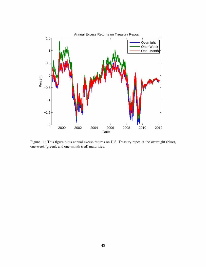
2000 2002 2004 2006 2008 2010 2012−2

−1.5

−1

−0.5

0

0.5

1

1.5Annual Excess Returns on Treasury Repos

Date

Per

cent


Figure 11: This figure plots annual excess returns on U.S. Treasury repos at the overnight (blue),one-week (green), and one-month (red) maturities.

48

1998 2000 2002 2004 2006 2008 2010 2012−2

−1.5

−1

−0.5

0

0.5

1Quarterly Excess Returns on MBS−Treasury Repo Spreads

Date

Per

cent


Figure 12: This figure plots quarterly excess returns on the spreads between mortgage-backed se-curity and U.S. Treasury repo rates at the overnight (blue), one-week (green), and one-month (red)maturities.

49

1998 2000 2002 2004 2006 2008 2010 20120

200

400

600

800Policy Uncertainty Index

Date

1998 2000 2002 2004 2006 2008 2010 20120

20

40

60

80

100VIX

Date

Figure 13: This first panel of this figure plots the Bloom et. al. (2012) policy uncertainty index fromSeptember 1997 to January 2012 at the daily frequency. The second panel of this figure plots theSP VIX index from September 1997 to January 2012 at the daily frequency.

50

risk premia in the repo market - new york university

Documents