Risk Overhang and Loan Portfolio Decisions: Small Business Loan Supply Before and During the Financial Crisis

Robert DeYoung, University of Kansas Anne Gron, NERA Economic Consulting

Gokhan Torna, State University of New York at Stony Brook Andrew Winton, University of Minnesota

This draft: April 22, 2014

Abstract: We find evidence that community banks restricted credit to small and medium sized enterprises in the U.S. during the global financial crisis. We estimate a structural model of bank portfolio lending with market imperfections, and exploit two sources of exogenous within-sample variation to identify our tests. Banks became less tolerant of risk during the crisis as loans became more difficult to sell and equity capital more expensive, resulting in pro-cyclical risk overhang effects. Our findings are consistent with crisis-era studies of European bank lending, but go further by showing that these behaviors can be explained by financial intermediation theory.

The opinions expressed in this paper do not necessarily reflect the views of NERA Economic Consulting. We thank three anonymous referees, the journal editor, Allen Berger, Lamont Black, Paolo Fulghieri, Ted Juhl, Greg Udell and seminar participants at Bangor University, the Bank of Canada, the Federal Deposit Insurance Corporation, the Federal Reserve Bank of Chicago, the University of Groningen, the University of Kansas and the University of Limoges for their insightful comments and suggestions.

1. Introduction

Small businesses, defined as having less than 500 employees, employ about one-half of the U.S.

labor force and create nearly two-thirds of net new private sector jobs in the U.S. annually (U.S. Small

Business Administration, 2012). Virtually all of these small firms are privately held and lack access to

public capital markets. To ensure access to credit, these informationally opaque businesses establish

close borrower-lender relationships with small, so-called ‘community banks’ (e.g., Petersen and Rajan

1994; Berger, Saunders, Scalise, and Udell 1997; Berger, Miller, Petersen, Rajan and Stein 2005). This

confluence of small firms and small banks is uniquely important for macro-economic growth both in the

U.S. and elsewhere: Berger, Hasan, and Klapper (2004) found a strong positive link between a large,

healthy small banking sector and macro-economic growth across 49 developed and developing nations.

The financial crisis took a toll on the U.S. small banking sector. About 6% of for-profit

depository institutions (commercial banks and thrift institutions) failed between 2007 and 2012, and 411

of those 478 insolvencies were small institutions with assets less than $1 billion (http://www.fdic.gov). It

is understandable that small business clients of these failed institutions would suffer interruptions,

reductions or even outright loss of their credit lines as the FDIC fashioned resolutions for these banks.1

But it remains an open question whether the stress of the financial crisis caused healthy banks in the U.S.

to reduce the amount of new credit they supplied to small and medium enterprises (SMEs). A reduction

in SME credit supply by healthy banks—that is, a credit crunch or credit rationing—would have pro-

cyclical effects, exacerbating the economic downturn by denying firms the short-term credit necessary to

finance increased inventories and retain workers. Moreover, credit rationing by small banks would be

antithetical to the whole idea of a banking relationship, which carries with it the presumption that

additional credit will be available when needed. In this paper, we investigate whether, how and why

small U.S. banks reduced their supply of credit to small businesses during the financial crisis.

1 The FDIC arranged ‘purchase and assumption’ resolutions for 427 of these failed banks. In these transactions, the FDIC arranges for a healthy bank to acquire all of the assets of the failed bank, so clients of these failed bank were unlikely to fully lose access to credit. In the other 51 bank insolvencies, the FDIC seized the failed bank’s assets and disposed of them piecemeal over time; clients of these banks were more likely to fully lose access to new credit.

1

Some evidence has emerged—mainly from European economies where credit registries provide

researchers with highly detailed data on loans and loan applications—that the financial crisis was

accompanied by reduced credit supply to SMEs (e.g., Popov and Udell 2010; Cotugno, Monferra and

Sampagnaro 2012; Jimenéz, et al 2012). These studies document that credit supply declined more during

the crisis at banks experiencing financial stress (low levels of equity capital, poorly performing loan

portfolios) but declined relatively less for SMEs with strong bank-borrower relationships. While this

body of research is informative and in some cases impressive, it remains incomplete. First, none of the

extant research examines credit to U.S. small businesses. By necessity, U.S. research has focused on the

syndicated loan supply to large firms during the crisis (e.g., Ivashina and Scharfstein 2010a, 2010b)

because systematic loan-level data for SMEs are not available. Given that the business, banking and

financial environments in the U.S. and Europe are substantially different, one cannot simply assume that

small business credit supply behaved similarly on both sides of the Atlantic. Second, the extant studies

employ pure empirical methodologies and ad hoc econometric test specifications. While these studies

find well-identified statistical associations between financial conditions and SME credit supply, they

leave un-modeled and unexplained the behavioral phenomena that drive these empirical associations and

the channels through which these associations occur. In order to successfully prevent credit supply

inefficiencies during recessions, policymakers need to know not just whether the actions of small business

lenders help perpetuate the downturn, but more importantly why and how this pro-cyclical behavior

occurs. We address both of these shortcomings in the extant literature, using data from small U.S.

commercial banks to estimate a structural econometric model of loan supply to small business firms.

We estimate a small business loan supply model for U.S. commercial banks both before and

during the financial crisis. Because loan-level data for SME loans are not systematically available in the

U.S., we use lender-level data from small U.S. commercial banks. These banks are not large enough to

make or even participate in loans to large firms; all of their new business loan originations, as well as all

of their business loans held in portfolio, are SME loans. Having limited our sample in this way, the

observed quarter-to-quarter change in bank-level business loans become a natural measure of net new

2

SME loan supply. We base our empirical loan supply equation closely on the theoretical loan supply

function, which we derive from a bank loan portfolio model in which market imperfections (illiquid

loans, costly external capital) make bank lenders effectively risk averse (Froot, Scharfstein and Stein,

1993; Froot and Stein, 1998). Thus, in the course of testing empirically whether U.S. banks reduced

and/or rationed credit to SMEs during the global financial crisis, we also perform an important empirical

test of financial intermediation theory.

Froot, Scharfstein and Stein (1993) predict that, when external finance is costly, value-

maximizing firms make investment decisions in a risk-averse manner: they base decisions not only on the

expected returns from the investment opportunity in question, but also on their stock of available

investment capital and the new investment’s return covariance with the rest of their business. These

considerations increase a firm’s expected profits by reducing the probability that it will forego a valuable

future investment opportunity when the return on the prospective investment does not justify the costs of

raising additional external capital—either because the firm has too little internal capital to make the

investment or it is unable to free-up internal capital by selling off lower yielding assets because they are

illiquid.

Froot and Stein (1998) apply this theory to banks. In their role as delegated monitors, banks have

private information that makes their loans relatively or completely illiquid, which leads to the central

implications of our theory model: if existing loans are illiquid and cannot be cheaply sold off, and if the

returns on these existing exposures positively covary with the returns on business loans, then capital

constrained banks will make fewer new business loans. Similarly, if a bank with largely illiquid existing

loans suffers a reduction in its equity capital, then the bank will also make fewer new illiquid loans. We

refer to these phenomena as ‘risk overhang’ or ‘loan overhang’ effects (Gron and Winton 2001). These

effects should grow stronger during economic downturns—during which preexisting loans become both

riskier and more illiquid, and equity capital both shrinks and becomes more costly—and as a result bank

lenders will become effectively more risk averse. Should we find that small banks did reduce their supply

of credit to SMEs during the financial crisis, then our theory provides several testable hypotheses about

3

the motivations for doing so and the channels through which it was done.

The assumptions upon which we base our theory model are especially appropriate for SME

lending by small banks. SME loans are illiquid assets and must be held in portfolio where they lock up

equity capital. Small banks are seldom publicly traded, rarely have public credit ratings, and face

relatively inelastic deposit markets,2 all of which make external capital expensive. Small bank

shareholders tend to be poorly diversified—ownership is often concentrated within a single extended

family, with a disproportionate share of owners’ wealth invested in the bank (Spong and Sullivan 2007)—

which further encourages risk-averse business practices. Likewise, the financial crisis provides a natural

environment for testing the predictions of our theory model: bank equity capital became more costly,

financial markets became less liquid, and (casual empiricism suggests) lenders became more risk averse.

We test the loan supply predictions of our model for a panel of quarterly data on U.S. banks with

assets less than $2 billion (2010 dollars) operating in metropolitan and urban markets between 1991 and

2010. We use a standard 2SLS-IV estimation approach—with bank fixed effects, time fixed effects, and

theoretically consistent economic conditions variables to absorb variation in local loan demand—to

account for the simultaneity of banks’ new SME loan supply decisions with their new lending decisions

in other loan sectors (consumer loans, real estate loans). We gain identification by embedding two

separate difference-in-differences frameworks into the empirical supply equation, which we specify using

exogenous variation in the market imperfections central to our model: exogenous bank-specific

differences in loan liquidity and exogenous bank-specific differences in the cost (availability) of external

equity capital.

For our first source of exogenous variation we exploit differences in bank corporate organization

form. Banks organized as subchapter S corporations do not pay corporate income tax, but they are

required to regularly distribute a large portion of their net income to shareholders as dividends, where

personal income tax rates are then applied to the income. Moreover, tax law places an upper limit on the

number of shareholders in an S corporation. Hence, external capital is especially costly for subchapter S

2 For evidence that bank deposit markets are fairly inelastic, see Amel and Hannan (1999).

4

banks. According to our theory, a shock to personal income tax rates in the home states of S corporation

banks should result in especially strong loan overhang effects. Our empirical tests confirm this

expectation. For our second source of exogenous variation we exploit differences in bank business

strategies. At small banks, loans to small companies (e.g., SME business loans, commercial real estate

loans) are informationally opaque and especially illiquid, but loans to households (e.g., consumer loans,

mortgage loans) are relatively less illiquid because these loans are often securitizable. Hence, the loan

portfolios of banks with long-established “commercial focused” lending strategies will be more illiquid

than banks with other business strategies. According to our theory, a shock to the cost or availability of

external capital (i.e., the onset of the financial crisis) should result in especially strong loan overhang

effects at these banks. Our empirical tests also confirm this expectation.

On average, our empirical results indicate that small U.S. banks reduced their supply of credit to

SMEs during the financial crisis. Moreover, these findings look like credit rationing: we find a strong

positive relationship between net new SME lending and the expected returns on SME loans prior to the

crisis, but after the onset of the crisis SME loan supply becomes insensitive (perfectly inelastic) on

average to expected loan returns. However, the small segment (about 13%) of the banks in our data with

commercial focused lending strategies supplied increased amounts of credit to small businesses during

2008 (the first full year of the crisis) and then maintained this higher level of SME credit supply during

both 2009 and 2010. These results imply that borrower-lender relationships help mitigate credit supply

shocks to small businesses, consistent with the findings of non-U.S. studies based on loan-level data

(Cotugno, Monferra and Sampagnaro 2012 for Italian banks; Liberti and Sturgess 2012 for a single

multinational lender).

Our results are largely consistent with the predictions of our theory. We find strong evidence of

loan overhang effects. All else equal, banks make fewer new business loans when their portfolios contain

large amounts of preexisting business loans, and make more new business loans when their portfolios

contain large amounts of loans to other sectors (e.g., consumer loans) that covary negatively with business

loans. These loan overhang effects grew stronger during the financial crisis, consistent with reductions in

5

loan liquidity and lender risk tolerance during an economic downturn. We also find strong evidence

consistent with the theoretical ‘risk tolerance’ predicted by our model, in which the new supply of illiquid

loans varies positively with fluctuations in a bank’s equity capital. Prior to the crisis, a decrease in a

bank’s equity capital cushion is associated with a reduction in new business loan supply. During the

crisis, this risk-averse lending behavior continues for well-capitalized banks, but it disappears for banks

with less equity capital. While the latter result is consistent with the literature on risk-seeking behavior at

poorly capitalized banks (Merton 1977, Marcus 1984), it may simply indicate that rebuilding their equity

capital bases was the paramount objective for poorly capitalized banks during the crisis, thus

disconnecting for a time their capital levels from their new lending decisions.3

While our results confirm the main findings of previous studies of small business lending during

the financial crisis—namely, that supply-side phenomena were important drivers of reduced credit

availability for SMEs—we also extend this body of knowledge in a number of ways. First, our

econometric methodology allows us to estimate the impact of the financial crisis on SME lending in the

U.S., even in the absence of loan-level data. Second, by using theory to inform these empirical tests, we

are able to empirically identify some of the meta-drivers of SME lender behavior, i.e., loan illiquidity,

equity capital supply and lender risk aversion. Third, we find that these determinants of SME loan supply

vary in strength across the business cycle, consistent with models of pro-cyclical bank lending driven by

internal bank behavior (e.g., Rajan, 1994; Berger and Udell, 2004; Ruckes, 2004; Repullo and Suarez,

2013). Risk overhang effects are pro-cyclical: small business loan supply declines during economic

downturns by even more than would be implied by recessionary reductions in bank capital alone. When

loan securitization markets broke down during the financial crisis, banks were less able to sell their

outstanding stocks of real estate and consumer loans, and this increase in loan portfolio illiquidity tied up

equity capital that could otherwise have been used to back new small business lending. When declining

stock market conditions (lower prices, higher price volatility) made issuing new risk capital more

3 Differentiating between these two possible explanations lies beyond the scope of this study.

6

expensive, banks became more circumspect (effectively more risk averse) when allocating their existing

risk capital, which exacerbated extant loan portfolio overhang effects and made banks less likely to

extend new business credit at the margin.

The plan of the paper is as follows. In Section 2 we review the previous research studies that are

most relevant for our investigation. In Section 3 we derive a theoretical loan supply function from a

model of bank loan portfolio allocation with capital market imperfections. In Section 4 we make some

adjustments to the theoretical loan supply equation to make it suitable for empirical estimation and

hypothesis testing. In Section 5 we show that community banks in the U.S. have characteristics that

comply closely with the maintained assumptions of our theory model, and as such provide a natural venue

for testing its predictions for SME loan supply. In Section 6 we present the data and variables used in our

regression models. In Section 7 we describe our empirical identification schemes. In Section 8 we

present the results of our main regression tests and robustness tests. In Section 9 we summarize our

findings and discuss their implications for policy.

2. Related literature

A large body of empirical studies investigate whether implementation of the Basel I capital

requirements caused a credit crunch in the U.S. (e.g., Bernanke and Lown 1991, Hall 1993, Haubrich and

Wachtel 1993, Berger and Udell 1994, Hancock and Wilcox 1993, Brinkman and Horvitz 1995, Peek and

Rosengren 1995). In general, these studies relate loan growth to capital measures and other controls.

Although this literature does not generate a consensus on the relationship between bank capital and loan

supply, Sharpe (1995) identifies two robust results across the studies: bank profitability has a positive

effect on loan growth, and loan losses have the opposite effect. Since profits (loan losses) tend to increase

(decrease) bank capital, these findings are consistent with a positive bank capital-loan growth link. In

more recent work, Beatty and Gron (2001) find that banks with stronger capital growth have greater loan

growth, with the most significant effects coming from the most capital-constrained banks.

The global financial crisis has motivated a new stream of studies on bank capital and bank loan

7

supply. Perotti, Ratnovski and Vlahu (2011) derive a non-monotonic theoretical relationship between

bank capital and bank risk-taking. When banks are operating near their regulatory capital minimums,

additional capital results in fewer tail risk projects (consistent with a reduction in the value of the deposit

put option, e.g., Merton 1977, Marcus 1984). However, when capital is so high that banks have no worry

of breaching their regulatory capital minimums, additional capital results in more tail risk projects; hence,

capital supports risk tolerance. Empirical studies by Black and Hazelwood (2011), Duchin and Sosyura

(2010) and Li (2011) all find at least some evidence of increased lending (i.e., greater risk-taking) at

banks that received government capital injections, while Carlson, Shan and Warusawitharana (2011) find

bank lending during the financial crisis was most sensitive to increases in capital at banks with low capital

ratios. These findings have obvious policy implications; however, because they focus narrowly on bank

lending behavior in response to artificial (non-market) capital injections during a period of severe

financial stress, they provide an incomplete treatment of the bank capital-loan supply relationship.

Much of our current knowledge about the impact of the financial crisis on small business loan

markets comes from European economies, where credit registries provide researchers with highly detailed

data on loans and loan applications. Jimenéz, Ongena, Peydro and Saurina (2012) find that reductions in

business lending in Spain during the financial crisis were predominantly caused by supply-side effects

due to weak bank balance sheets, rather than demand-side forces. Popov and Udell (2010) find that both

supply-side and demand-side factors led to reduced SME lending in 14 European countries: banks

experiencing stress to their assets and equity values extended less credit, and high-risk SMEs with fewer

tangible assets received less credit, during the early stages of the financial crisis. Cotugno, Monferra and

Sampagnaro (2012) find that SMEs in Italy experienced reduced credit supply during the financial crisis,

but that credit rationing was substantially mitigated for loan applicants with exclusive borrowing

relationships with their banks.

Research on U.S. bank lending during this period tends to use data on large business lending.

Ivashina and Scharfstein (2010a, 2010b) show that shocks to bank liquidity (e.g., deposit withdrawals,

credit line draw downs) were associated with reduced lending to large corporate customers during the

8

crisis. Montorial-Garriga and Wang (2012) derive a model of bank loan pricing with endogenous credit

rationing, and estimate it using a sample of U.S. bank loans during the 2000s; the authors conclude that

large business borrowers were less likely than small firms to be rationed out of the bank loan market

during the financial crisis. Garcia-Appendini and Montoriol-Garriga (2011) show that large, liquid firms

provided increased trade credit to their customers during the crisis, perhaps substituting for a reduction in

credit supply from banks.

Our study differs from the previous literature in several respects. First, while most previous

studies focused on large banks, we focus exclusively on small banks to ensure that the loan supply we are

observing is going to small businesses. Second, previous studies estimated reduced-form regression

models, whereas we estimate a structural econometric model based on a theory of loan supply that is

highly descriptive of the opportunities and constraints facing small bank lenders. Third, most previous

studies used annual data over a limited period of time, whereas we observe detailed changes in portfolio

composition and loan supply at quarterly intervals over 20 years. Observing data at these more frequent

quarterly intervals is essential for testing the loan portfolio hypotheses in our theory model. Fourth,

within the small set of studies that test the impact of the financial crisis on bank lending, we are the first

to examine this question exclusively for small business lending in the U.S. Finally, and perhaps crucially,

we are able to empirically identify the relationships between SME loan supply and bank balance sheet

conditions and lending behavior (e.g., loan overhang, loan illiquidity, risk tolerance) without access to

either loan-level data or a convenient natural experiment.

Our work is rooted in the theoretical literature that models financial institution portfolio

management when external financing is costly due to capital market imperfections. These theories apply

particularly to banks with enough equity so that moral hazard via risk shifting does not become an issue.4

4 It is well-known that banks with very low capital levels may engage in moral hazard via risk-shifting, possibly by overly aggressive lending, as in Marcus (1984). This is more likely if deposit insurance is priced at a flat rate. By contrast, if capital levels are not very low, banks may become more conservative in their lending when capital levels fall, as in Besanko and Kanatas (1996), Thakor (1996), Holmstrom and Tirole (1997), Diamond and Rajan (2000) and Perotti, Ratnovski and Vlahu (2011).

9

Froot, Scharfstein and Stein (1993) show that firms facing costly external finance, stochastic net worth,

and attractive future investment opportunities will behave in a risk-averse manner. Froot and Stein (1998)

extend this model to include the influence of preexisting portfolios of investments on financial institutions

new investment decisions. These authors show that the amount the institution will want to invest in a new

opportunity will depend upon its level of capital, the covariance of that investment’s cash flows with the

cash flows of the firm’s stock of illiquid (or non-tradable) asset exposures, and the covariance of the non-

tradable cash flows of any other new investments the firm is considering. Froot (2007) extends the

framework further in a model of insurance companies, introducing product market imperfections and

allowing some of the risks faced by insurers to be hedged. Several empirical applications of this

framework exist. Froot and O’Connell (1999) apply this model to price determination in the catastrophe

reinsurance market. They show that such financing imperfections can lead to costly reinsurer capital and

also to reinsurer market power, and estimate the corresponding supply and demand curves. Gron and

Winton (2001) use the term ‘risk overhang’ to describe how outstanding and illiquid risk exposure from

long-term insurance policies can affect the current supply of new insurance policies. In extreme cases,

increases in risk overhang may lead firms to reduce their total exposure to the underlying risk by

canceling existing policies.

3. Loan Supply with Capital Market Imperfections: Theory

In this section we develop a portfolio model of bank loan supply. We begin with a representative

bank which has lending opportunities in several sectors. Loans can be funded out of net internal capital

W or external funds F, where external funds are assumed to be more costly than internal funds. This

additional cost reflects information asymmetries between the firm and outside investors (e.g., Myers and

Majluf 1984, DeMarzo and Duffie 1999), as well as other transaction costs in accessing public markets.

In addition to current period loans, the bank may be able to make profitable loans in future periods. As

shown by Froot, Scharfstein and Stein (1993), profitable future investment opportunities combined with

costly external funds and stochastic internal funds cause the firm's objective function to be increasing and

10

generally concave in the stock of internal funds. Intuitively, more internal funds lessen the extent to

which a bank must rely on costly external funds, but this benefit is generally decreasing because, at the

margin, there are fewer profitable uses for these funds. Denoting the indirect form of the bank's objective

function as P(W), we have PW > 0 and PWW < 0 where the subscript denotes the partial derivative.

The bank begins period t with Wt-1 in net internal funds, Lt-1,i in outstanding loans in each sector i,

and net external finance of Ft-1=∑i (Lt-1,i) -Wt-1 > 0. For simplicity, we assume that all external finance

takes the form of debt.5 For the moment, assume that all of the bank’s outstanding loans are illiquid and

cannot be sold due to the bank’s private information on loan quality. Since the bank must bear the risk of

Lt-1,i loans in each sector i regardless of its subsequent decisions in period t, Lt-1,i is the bank’s risk

overhang in sector i in period t.

During period t the bank can make new loans NLt,i ≥ 0 to each sector i, resulting in end-of-period

outstanding debt of Ft = ∑i (Lt-1,i+ NLt,i) - Wt-1. The gross per dollar cost of debt funding is 1+rt, which

includes any costs of accessing external markets rather than using internal capital. During period t, the

bank realizes the gross per dollar return of 1/,~

−titR on loans to sector i that were originated in period t-1.

1/,~

−titR equals 1+rt+pt-1,i-η~ t,i, where pt-1,i is the per dollar credit spread or markup charged on sector i loans

that originated in period t-1, and η~ ti is the random per dollar loan losses on sector i loans in period t.

Similarly, the bank realizes the gross per dollar return titR /,~ = 1+rt+pt,i-η~ t,i on the new loans to sector i

5 Regardless of its form, external finance is costly for banks. In the presence of binding (or even close to binding) minimum regulatory capital requirements, banks must raise external debt in combination with new equity. Indeed, Berger, DeYoung, Flannery, Lee and Oztekin (2008) show that when commercial banks fall closer to their regulatory minimums, they actively manage their capital to return quickly to their internal capital targets. Issuing new equity involves significant transaction and informational costs, especially for banking companies that are not publicly traded (the majority of the industry). For banks that are not too-big-too-fail (again, the majority of the industry), issuing subordinated debt or large denomination deposit contracts also entails such costs. And although (non-TBTF) banks can issue federally insured retail deposits that would seem to be unaffected by such information concerns, there is evidence that these debt contracts are not perfect, costless substitutes for uninsured debt. Billett et al. (1998) find that large banks increase their use of insured deposits following downgrades of their publicly traded debt, but also find that total debt finance (insured plus uninsured liabilities) declines, consistent with increased external costs of debt finance. Further support that external funding is costly for banks comes from Jayaratne and Morgan (2000), who find that banks finance an unusually large portion of their assets with internal funds. Finally, Amel and Hannan (1999) show that markets for insured deposits are relatively price inelastic, indicating that banks cannot raise large additional amounts of these funds without significantly increasing the rate they pay.

11

originated in period t, where pt,i is the per dollar credit spread on these loans. For simplicity, we assume

that all losses on loans to sector i borrowers in period t are perfectly correlated, regardless of when the

loan was made. Current period loan losses are assumed to be normally distributed: ),(~~,,, ititit N σµη

where both μt,i and σt,i depend on the sector’s economic outlook at the start of that period.6 Both μt,i and

σt,i are decreasing in the sector's economic outlook: when borrowing firms have better prospects, both ex

ante credit risk and ex post realized loan losses are lower because the borrowing firms’ chances of default

are reduced. Given these assumptions, it follows that the bank’s net capital at the end of period t is

)]~()~([)1(

)1(]~~[~

,,,1

,,1,10

/,,1

1/,,1

ititit

n

iitititt

tttitit

n

itititt

pNLpLrW

rFRNLRLW

ηη −+−++=

+−+=

∑

∑

=−−

=−−

(1)

where we have made use of the definitions of 1/,~

−titR , titR /,~ , and Ft.

The bank chooses new loan amounts NLt,i that maximize expected profit E[P( tW~ )], given the

financing constraints. This leads to the first order condition for each sector i

)~,()]([)]~([]~

[0 ,,,,,,

itWititWititWit

tW PCovpPEpPE

NLWPE ηµη −−=−=

∂∂

= , (2)

where we have made use of (1) and the identity E(xy) = E(x)E(y) + Cov(x,y). Since loan losses it ,~η and

the level of internal funds tW~ are both normally distributed, we can apply Stein’s Lemma and the

definition of covariance to derive the bank’s supply of new loans SitNL , to sector i 7

.1 ,,,1,1,,

ii

itit

ii

ijij jtit

ii

ijSjtij

Sit

pG

LLNLNLσ

µσσ

σσ −

⋅+−−−= ∑∑ ≠ −−≠ (3)

6 In reality, loan losses are skewed to the right: they cannot be less than zero, there is a high probability that they won’t be too large, and a low probability of very large losses. The assumption of normality allows us to give a simple, tractable analytic solution to the bank’s portfolio choice problem. 7 Stein’s lemma implies Cov(PW, it,

~η ) = E[PWW]Cov( tW~ , it,~η ). We also use Cov( tW~ , it,

~η ) =

ji)σj jtNLjt(L ,,,1∑ +−− .

12

where for convenience we have suppressed the time subscript on the loan performance variance and

covariance terms. In (3), σii is the variance of loan losses in sector i over time; σij is the covariance of loan

losses across sectors i and j over time; ][][

W

WW

PEPEG −= measures the bank’s effective risk aversion

induced by the costs of external finance, and hence we shall refer to its reciprocal 1/G as the bank’s risk

tolerance.

The bank’s supply of new loans to sector i is determined by several factors on the right-hand side

of equation (3). The first term is the effect of covariance-adjusted lending opportunities in other sectors

j≠i at time t. The second term is the preexisting portfolio exposure in sector i, that is, the overhang of

outstanding loans in sector i at time t. The third term is the effect of the covariance-adjusted loan

overhangs in other sectors j≠i. The final term is the bank’s tolerance 1/G multiplied by the risk-adjusted

profit ratio (pt,i-μt,i)/σii. It is straightforward to verify that equation (3) has the features of a supply curve.

The supply of new loans to sector i is increasing in the current credit spread (or ‘markup’) pt,i and

decreasing in expected loan losses (or costs) μi,t. Assuming that pt,i exceeds μt,i, new loan supply is also

decreasing in the bank’s effective risk aversion G. Further, the supply of new loans to sector i is

decreasing in the overhang of outstanding loans in that sector, Lt-1,i. Finally, if the covariance between

sector i and sector j is positive, then the supply of new loans in sector i is decreasing in both the overhang

of outstanding loans in sector j and the supply of new loans in sector j; by contrast, if the covariance is

negative, then the supply of new loans in sector i is increasing in loans to sector j.

4. Loan Supply with Capital Market Imperfections: Issues for Empirical Specification

Equation (3) forms the basis for our empirical analysis. Before estimating this model, we must

make adjustments for two features of the banking data that are not perfectly consistent with the theoretical

assumptions above: some bank loans are not perfectly illiquid, and new loan supply is not directly

observable.

4.1. Banks hold liquid and illiquid loan stocks

13

During a given accounting period, some loans will mature and be repaid. The remaining loan

stocks exhibit varying degrees of liquidity. As shown by Froot and Stein (1998), under optimal portfolio

allocation with imperfect capital markets, it is optimal for banks to shed all loans that can be sold at fair

value. However, due to information asymmetries or transactions costs, the market prices of loans may be

less than banks’ expected values, resulting in illiquid loans which banks hold rather than sell.

Let δt-1,i ∈(0,1) be the illiquid portion of the outstanding loans at the beginning of period t (end of

period t-1). The remaining loans are assumed to be liquid and will be sold off at no cost, or will run off

naturally, to make room for new loans. Since only illiquid loan stocks will affect new lending, we can

rewrite equation (3) as

ii

itit

ii

ijij jtjtitit

ii

ijSjtij

Sit

pG

LLNLNLσ

µσσ

δδσσ ,,

,1,1,1,1,,1 −

⋅+∑−−∑−= ≠ −−−−≠ (3′)

where we have substituted the illiquid stock of outstanding loans δt-1,iLt-1,i and δt-1,jLt-1,j in place of the total

(liquid and illiquid) stock of outstanding loans Lt-1,i and Lt-1,j. Unfortunately, while equation (3') is the

theoretically correct relationship, we cannot observe the fractions δt-1,i and δt-1,j in the available banking

data. Thus, although the theoretical equation (3') predicts that the coefficient on the outstanding (illiquid)

same-sector loan stock variable (δt-1,iLt-1,i) will be exactly -1 (that is, every dollar of illiquid loans causes

the bank to forgo one dollar of new loans), in our regressions the estimated coefficient on the total

outstanding same-sector loan stock variable (Lt-1,i) will simply absorb the theoretical illiquidity term δt-1,i.

Thus, we would expect the estimated regression coefficients on Lt-1,i and Lt-1,j to be larger (i.e., closer to 1

in absolute value) as these outstanding loan stocks become more illiquid.

The degree to which outstanding loans are liquid or illiquid is not fixed but can change with

exogenous conditions. For example, a recession may reduce the liquidity of outstanding loans: borrowers

will be more likely to roll over rather than repay drawn down credit, and increased adverse selection

problems make it more costly for banks to sell or securitize loans. Additionally, a recession may have a

capital effect: with the expectation of increased future losses on outstanding loans—and thus lower equity

capital levels in the future—banks will become more risk averse lenders.

14

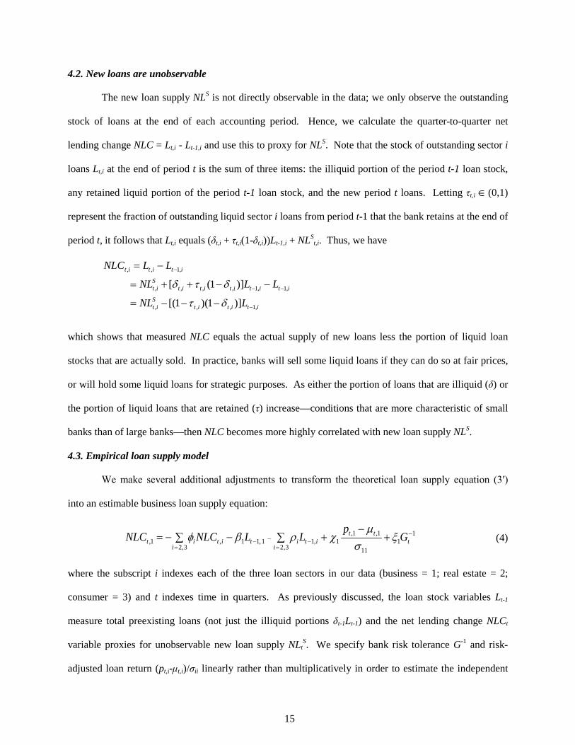
4.2. New loans are unobservable

The new loan supply NLS is not directly observable in the data; we only observe the outstanding

stock of loans at the end of each accounting period. Hence, we calculate the quarter-to-quarter net

lending change NLC = Lt,i - Lt-1,i and use this to proxy for NLS. Note that the stock of outstanding sector i

loans Lt,i at the end of period t is the sum of three items: the illiquid portion of the period t-1 loan stock,

any retained liquid portion of the period t-1 loan stock, and the new period t loans. Letting τt,i ∈(0,1)

represent the fraction of outstanding liquid sector i loans from period t-1 that the bank retains at the end of

period t, it follows that Lt,i equals (δt,i + τt,i(1-δt,i))Lt-1,i + NLSt,i. Thus, we have

itititS

it

itititititS

it

ititit

LNL

LLNL

LLNLC

,1,,,

,1,1,,,,

,1,,

)]1)(1[(

)]1([

−

−−

−

−−−=

−−++=

−=

δτ

δτδ

which shows that measured NLC equals the actual supply of new loans less the portion of liquid loan

stocks that are actually sold. In practice, banks will sell some liquid loans if they can do so at fair prices,

or will hold some liquid loans for strategic purposes. As either the portion of loans that are illiquid (δ) or

the portion of liquid loans that are retained (τ) increase—conditions that are more characteristic of small

banks than of large banks—then NLC becomes more highly correlated with new loan supply NLS.

4.3. Empirical loan supply model

We make several additional adjustments to transform the theoretical loan supply equation (3′)

into an estimable business loan supply equation:

11

11

1,1,1

3,2,11,11

3,2,1,

−

=−−−

=+

−+∑−∑−= t

tt

iitit

iitit G

pLLNLCNLC ξ

σµ

χρβφ (4)

where the subscript i indexes each of the three loan sectors in our data (business = 1; real estate = 2;

consumer = 3) and t indexes time in quarters. As previously discussed, the loan stock variables Lt-1

measure total preexisting loans (not just the illiquid portions δt-1Lt-1) and the net lending change NLCt

variable proxies for unobservable new loan supply NLtS. We specify bank risk tolerance G-1 and risk-

adjusted loan return (pt,i-μt,i)/σii linearly rather than multiplicatively in order to estimate the independent

15

effects of these measures.8 The regression coefficients φ, β, ρ, χ and ξ are parameters to be estimated.

The coefficients φ and ρ absorb (and hence will reflect) the effects of the suppressed covariance-variance

ratios σij/σii while the coefficients β and ρ absorb (and hence will reflect) the unobserved liquidity effects

δt and τt as discussed above.

In our estimations, we additionally control for fixed bank effects, fixed time effects, and

economic conditions in banks’ local markets. Since banks make new business loan supply decisions

simultaneously with new real estate and consumer loan supply decisions, the right-hand side NLCt,i terms

are endogenous, and we account for this by estimating equation (4) using two-stage instrumental variables

techniques. Full details of our estimation methods appear below.

4.4. Predicted signs for estimated coefficients

Based on the discussion above, we can make the following predictions about the estimated

coefficients of equation (4):

• Same-sector loan overhang: Within the business loan sector, net lending change will be negatively

related to overhang (β1<0). This effect will be stronger when the sector is less liquid.

• Cross-sector loan overhang: If the portfolio model is the primary determinant of net lending

changes, then the impact of cross-sector loan overhang on net lending change (ρji) will be

increasingly negative (or less positive) as the covariance between loan losses in sectors i and j

increases. Holding covariance constant (and not equal to zero), the magnitude of ρji will be larger the

more illiquid is loan stock j.

• Cross-sector net lending change: If our model holds strictly, the estimated effect of net lending

change in sector j on net business lending change (φji) should be the same sign as the estimated effect

of sector j loan stocks on net business lending change (ρji). The coefficients will be exactly the same

(φji=ρji) only if the loan stocks and net lending change have the same degree of liquidity and if loan

losses for each have the same correlation with loan losses for the net business lending change.

8 Estimating the model in its multiplicative form yields only trivial differences in the other coefficients.

16

• Risk tolerance: Within the business loan sector, net lending change will increase with the bank’s risk

tolerance (ξ>0).

• Risk-adjusted loan return: Within the business loan sector, net lending change will increase with the

risk-adjusted return ratio (χ>0). Effectively, this coefficient captures the risk-adjusted slope of the

business loan supply function.

5. Market imperfections and small bank lenders

The assumptions underlying our theory (i.e., imperfect capital markets, loan illiquidity, risk

averse lending decisions) are especially descriptive of the business lending environment faced by small

commercial banks. The limited lending capacity of these banks precludes them from making or

participating in business loans to large publicly traded firms; instead, small banks specialize in business

loans to small, privately-held businesses that are opaque to public capital markets. These loans typically

rely on relationships between a small bank’s loan officers and its business borrowers that allow the bank

to observe soft (i.e., not quantifiable) information about the borrower that can be used to evaluate the

borrower’s creditworthiness (Stein 2002). Although relationship loans are not based solely on soft

information—for example, banks usually require collateral for which a hard value can be determined—

these loans remain far less liquid than loans based solely upon quantifiable information.9 They are not

securitizable and can be sold to other banks only at large discounts, because the informational value of the

borrower-lender relationship cannot be credibly conveyed to outside investors. Moreover, when a bank

makes a relationship loan it knows that such an option does not exist—the exit barrier created by these

loans serves as an entry barrier for (larger, hard information-based) lenders that wish to avoid the

illiquidity that comes with relationship lending. Berger et al. (2005) find evidence consistent with this

9 While a large portion of these loans have short maturities, confusing maturity with liquidity belies the nature of the long-term borrower-lender relationship at the core of small banks’ business lending strategies. All else equal, community banks will be reticent to allow these loans to roll off their balance sheets, as this represents the loss of intangible relationship value in which the bank has invested. Moreover, as per Rajan (1992), the borrowers are likely to face informational lock-in costs if they try to repay their lender by seeking other sources of finance. Thus, the short (usually one-year) contractual maturities of small business credit lines are better interpreted as a risk-management tool that provides a periodic opportunity for adjusting loan terms and prices.

17

description.

Similarly, the real estate loans and consumer loans made by small banks may be less liquid than

those made by larger banks. Large banks originate with the intent to securitize large portions of their real

estate loans (e.g., residential mortgages, home equity lines of credit) and consumer loans (e.g., auto loans,

student loans, credit card receivables). The originate-and-securitize production process generates

additional costs that are not present in portfolio lending (e.g., legal and credit rating agency fees, overhead

for performing statistical analysis, establishing a reputation in the asset-backed securities market,

providing credit enhancements to the buyers of the asset-backed securities), but these additional expenses

may be more than offset by reduced expenses for credit screening, increased noninterest revenues (from

mortgage origination, servicing and securitization fees) and cost scale economies associated with this

production process. Because high volumes of loan origination are necessary to run this process

efficiently, and because selling off rather than holding loans is antithetical to close bank-borrower

relationships, small banks typically choose to securitize only a small portion of the real estate and

consumer loans they originate, and hold a larger portion as portfolio investments. The principle exception

to this are conforming home mortgage loans sold to government-sponsored enterprises such as Fannie

Mae, Freddie Mac and Ginnie Mae.

Small banks are also more likely to be sensitive to the risk overhang effects associated with

illiquid loan portfolios. These lenders lack access to public funding markets; this increases their cost of

external financing, which in turn magnifies the consequences of all new lending decisions. Because

credit derivatives are not a viable hedging strategy for these banks (CDS do not exist for small business

loans, and using existing CDS to hedge these loans would entail extreme basis risk), they must manage

risk in their loan portfolios by adjusting on-balance sheet loan concentrations. And small bank managers

are often placing their family’s capital at risk when making lending decisions (community banks are often

owner-managed), so risk-averse lending behavior should be relatively free of potentially confounding

principal-agent effects (DeYoung, Spong and Sullivan 2001; Spong and Sullivan 2007).

All of these small bank sensitivities likely grew stronger during the financial crisis, when access

18

to liquidity in general became tighter. Data from the fed funds market—a major source of short-run

liquidity for small and large banks alike—is indicative. Small U.S. banks (defined here as banks with less

than $2 billion in assets) tend to be deposit-rich, while large U.S. banks (defined here as banks with more

than $50 billion in assets) tend to be deposit-poor, and in normal times the fed funds market transfers

excess liquidity from small banks to large banks. Prior to the crisis, fed funds sold fluctuated between 3%

and 5% of small bank assets, but fell to only about 2% of small bank assets during the crisis. Similarly,

fed funds purchased fluctuated between 10% and 12% of large bank asset funding prior to the crisis, but

plunged to about 5% during the crisis. These two developments are strongly linked: the quarterly time

series correlation between small bank fed funds sold-to-assets and large bank fed funds purchased-to-

assets was 0.57 during the crisis (2008-2010); this correlation was -0.03 during the 17 years leading up to

the crisis. Hence, both large banks and small banks experienced unusual liquidity pressure during the

crisis: small banks felt it necessary to hold higher stores of precautionary liquidity, and this resulted in a

reduced supply of liquidity to large banks.

6. Data and variables

We estimate the model using quarterly financial statement data for small U.S. commercial banks.

These data are taken from the Federal Reserve’s Report of Condition and Income (call reports) database

from the first quarter of 1991 (1991: Q4) through the fourth quarter of 2010 (2010:Q4). This sample

period includes data from before and during the global financial crisis. We define the beginning and the

end of the crisis based on the small business lending behavior by U.S. banks reported in the Federal

Reserve’s Senior Loan Officer Opinion Survey on Bank Lending Practices (SLOOS). The SLOOS is

administered four times each year to a relatively stable set of around 55 large and medium sized U.S.

commercial banks. Among other questions, the survey asks each bank whether its credit standards for

approving small business loan applications have eased, remained unchanged, or tightened over the past

three months. Not surprisingly, banks reported that they tightened lending standards early in the crisis,

and reported that they eased lending standards as the crisis waned. The net percentage of banks

19

tightening their small business lending standards exceeded 10 percent for the first time in the January

2008 SLOOS, so we mark 2007:Q4 as the beginning of the crisis. The net percentage of banks easing

their small business lending standards exceeded 10 percent for the first time in the April 2011 SLOOS, so

we mark 2010:Q4 as the final quarter of the crisis.10 Hence, we refer to the 64 quarters of data from

1991:Q4 though 2007:Q3 as the ‘pre-crisis’ period and the 13 quarters of data from 2007:Q4 through

2010:Q4 as the ‘crisis’ period.

We apply three primary filters to select the banks in our data set. First, for the reasons stated

above, we include only small, so-called community banks with less than $2 billion in assets in real 2010

dollars.11 Second, we only include banks located in urban geographic areas (in SMAs); banks located in

rural areas face a different set of lending opportunities than urban banks, which results in different

exposures to loan overhang and different incentives for dealing with this risk.12 Third, we only consider

banks that make non-trivial amounts of business loans, real estate loans, and consumer loans—the three

main categories of loans reported in the call reports. We define these ‘non-specialist’ lenders each period

as follows: the dollar value of their sector i loans must be no more than ten times, and no less than one-

tenth, of the dollar value of either of their sector j loans (i≠j).13 As shown in Figure 1, the asset share of

10 In the January 2008 SLOOS, 17 banks tightened standards, 39 did not change their standards, and 0 eased their standards. Thus, the net percentage of banks that tightened standards = (17–0)/56 = 30.4%, up from just 9.6% in the previous survey. In the April 2011 SLOOS, 0 banks tightened standards, 45 did not change their standards, and 7 eased their standards. Thus, the net percentage of banks that eased standards = (7–0)/52 = 13.5%, up from just 1.9% in the previous survey. 11 For decades, both bank regulators and bank researchers used $1 billion as a convenient upper size threshold to define the U.S. community bank sector (DeYoung, Hunter, and Udell 2004). Our $2 billion threshold is similarly convenient, but recognizes several decades of inflation. 12 Rural banks typically have local market power; with greater rents at stake, their ability and willingness to absorb risk overhang may differ markedly from those of urban banks. The extreme localness, or ‘ruralness,’ of these banks influences the manner in which they underwrite loans and results in lower levels of credit risk (DeYoung, Glennon, Nigro and Spong 2011). Rural banks hold relatively low levels of total loans, high levels of marketable securities, and high levels of equity compared to similarly sized urban banks (DeYoung, Hunter, and Udell, 2004), consistent with a less sophisticated approach to risk management. And because the agricultural economy permeates the performance of all lending sectors at rural banks (e.g., business loans are dominated by agricultural production loans and loans to farm-related business concerns, and real estate loans include large amounts of farm mortgages and farm residential mortgages), the loan performance covariances will differ from those observed in urban markets. 13 These upper and lower boundary restrictions eliminated around one-third of the bank-quarter observations and became more binding over time. To test whether these restrictions introduced selection effects, we re-estimated our basic models using a data set that included both specialist and non-specialist lenders (not shown, results available upon request). In nearly all cases, the estimated coefficients carry the same signs, statistical significance, and order of magnitude as those generated using the non-specialist bank-only data set.

20

real estate loans for the average non-specialist bank approximately doubled during our sample period

before declining somewhat during the financial crisis; the asset share of consumer loans declined by about

half during our sample period; but the asset share of business loans remained relatively stable over time.14

As real estate loan shares increased, and consumer loan shares decreased, fewer banks qualified as non-

specialist lenders; hence, the number of observations in our tests unavoidably declines over time.

We make a number of additional adjustments to mitigate the potential effects of data errors,

merging banks, or banks with abrupt changes in lending strategies. We delete bank-quarter observations

in which the assets of another bank are acquired, bank-quarters when banks are less than 5 years old or

less than $25 million in assets, all observations for banks that lend out fewer than 25% of their assets, and

all observations for banks that were not present in the data for at least five consecutive quarters. We

delete bank-quarter observations when the ratio of nonperforming loans to beginning-of-period loans, the

ratio of net lending change to beginning-of-period assets, the quarterly change in assets, or the quarterly

change in equity capital are over the 99th percentile or below the 1st percentile of the sample distributions.

Similarly, we delete bank-quarter observations when the expected profit variable in any of the three loan

sectors is less than the 0.5th or greater than the 99.5th percentile of the sample distribution.

6.1. Regression variables

The empirical versions of the variables in theoretical loan supply equation (4) are defined in

Table 1. Descriptive statistics for these structural variables, as well as all other variables used in our

estimations, are displayed in Table 2. We define the existing stock of loans Lt-1,i for three categories of

loans: business loans (BUS), real estate loans (RE) and consumer loans (CON) and the end of quarter t-1.

Each of these three broad categories contains different types of loans; this high level of aggregation is

unavoidable given the structure of the call reports.15 BUS includes all commercial and industrial loans.

14 The sum of these three loan-to-asset shares increases over time. This mirrors the secular increase in total loan-to-asset ratios at small U.S. banks during the post-deregulation era, during which increased competition and industry consolidation removed inefficient banks that loaned out only a small portion of their assets (DeYoung, Hunter and Udell 2004, Tables A1 and A2). 15 While the call reports do disaggregate the portfolio balances for BUS, RE and CON loans into a variety of sub-categories, they do not similarly disaggregate the loan interest revenues associated with these sub-categories. This

21

RE includes all loans secured by a lien on real estate: commercial and development loans, first and second

mortgages on single family and multi-family residential properties, and mortgages on commercial

properties. CON includes all revolving, installment, or single payment loans to individuals (e.g., auto

loans, student loans, personal lines of credit), with the exception of credit card loans which we exclude

because they are relatively unimportant for small banks.16 We normalize BUS, RE and CON by end-of-

quarter t-1 bank assets to control for bank size. We define new lending supply NLSt,i (or net lending

change NLCt,i) for business loans (NEW_BUS), real estate loans (NEW_RE) and consumer loans

(NEW_CON) as follows: end-of-quarter t loan stock minus end-of-quarter t-1 loan stock, plus net loan

charge-offs (loans charged off minus loans recovered) during quarter t. Again, we normalize by t-1 bank

assets.17

The statistics displayed in Table 3, Panel B provide confirmation that business loans are on

average less liquid, and exhibit greater credit risk, than consumer and real estate loans. Credit risk data

are displayed in item 1. For the banks in our sample, business loans have the largest average quarterly

loan charge-off ratio (0.65%), followed by consumer loans (0.51%) and then real estate loans (0.10%).

This ranking is unchanged when specialist lenders are included in the averages. Although real estate

loans defaulted at high rates during the financial crisis, they have historically exhibited a relatively low

level of credit risk. Loan liquidity data are displayed in item 2. Unfortunately, the call reports do not

contain complete or uniform data on loan liquidity across loan types or across time. We use the sum of

the best variables available—“Outstanding principal balances of assets sold and securitized by the

reporting banks with serving retained or with recourse or other seller-provided credit enhancements” plus

“Assets sold with recourse of other seller-provided credit enhancements and not securitized by the

prevents us from calculating risk-adjusted loan returns (RAR) for loan sub-categories, and as such we are limited to using only the three highly aggregated loan categories in our tests. 16 Small banks exited credit card lending with the development of loan production processes (i.e., credit scoring and loan securitization) that exhibited huge scale economies. For the banks in our data, credit card loans never exceeded 1% of bank assets on average during our sample period. Loans to government entities, loans to other financial institutions, loans to finance agricultural production, and loans to finance the purchase of farm land also comprise a negligible portion of the loan portfolios of the small, urban banks in our sample. 17 In the theory model we assume that loans are perfectly illiquid and once made never leave the balance sheet. Hence, the theoretical term NL is non-negative. In contrast, our empirical proxies for NL are often negative because actual bank loans are only imperfectly illiquid, and can leave the balance sheet via sales, maturity, or charge-offs.

22

reporting bank”—to construct loan liquidity ratios for the second half of our sample. For the banks in our

sample, business loans are the least liquid ( 0.07%), followed by consumer loans (1.01%) and then real

estate loans (1.29%).18 Again, this ranking is unchanged when specialist lenders are included in the

averages.19

Specifying (pt,1-μt,1)/σ11 for business loans is an imperfect exercise and involves making some

choices. In our main tests, we define risk-adjusted returns on business loans (RAR) as the ratio of the

bank-specific expected returns on business loans in quarter t divided by the market-specific variance of

these returns over the preceding twenty quarter period. The numerator in this ratio is the expected percent

return (the bank’s interest and fee income from business loans during period t, divided by its stock of

accruing business loans at the beginning of period t) multiplied by the expected performance of business

loans (the within-state percentage of performing loans averaged over the preceding twenty quarters)

minus the average deposit rate paid by the bank (the interest paid on deposits during period t divided by

the average deposits in the current and prior period). The denominator in this ratio is the quarterly

variance of the within-state quarterly average of the numerator over the preceding twenty quarters. By

measuring loan performance and expected return variance at the market level, we capture average risk in

the pool of small businesses from which the bank is drawing its loans; this specification reduces (though

does not eliminate) problems associated with endogenous business loan returns. While we believe that

‘expected’ loan returns is the theoretically appropriate return concept, we also specify two other measures

of RAR: ‘realized’ loan returns and ‘perfect foresight’ loan returns. Appendix B contains detailed

definitions of these alternative RAR concepts and compares their performance in robustness tests of our

baseline models. There is no evidence that these alternative measures of RAR perform better than our

preferred RAR definition.

18 The small magnitudes of the liquidity ratios understate the extent of loan liquidity for two reasons. First, small banks do not sell loans continuously throughout the year; hence, in any given quarter, the average ratios contain lots of zeros. Second, these data report only loans for which the selling bank is still exposed to recourse or other credit guarantees, which often expire with a year after the loan has been sold. 19 Not surprisingly, the specialist lenders exhibit higher overall levels of both credit risk and loan liquidity. By specializing rather than diversifying, these banks (a) are signaling that they are willing to operate with higher levels of credit risk and (b) must rely more on loan sales to manage their risk profiles.

23

We define bank-specific risk tolerance G-1 as the bank’s total equity capital divided by its total

assets at the beginning of quarter t (EQ).20 Intuitively, banks with lower financial leverage (higher equity

capital) will in general be more risk tolerant in their lending decisions: they are better able to absorb loan

losses and better able to sustain increased illiquidity in any one loan sector without making compensating

adjustments in other portions of their loan portfolio.

Note that, because the preferences of bank managers are idiosyncratic, the intrinsic level of

managerial risk aversion may vary across banks, with more risk-averse managers holding more capital on

average and less risk-averse managers holding less capital on average. Our fixed effects estimation

techniques will absorb these cross-section differences. Thus, the estimated coefficient on EQ will reflect

how an increase (decrease) in capital relative to that bank’s average capital will create (deplete) a capital

cushion and allow the bank to act in a more (less) risk tolerant fashion.

6.2. Loan performance covariances

In our theory model (3), the cross-sector overhang effects of non-business loans on new business

loan supply are explicitly related to the sign of the loan performance covariances (σij). In our empirical

model (4), however, the influence of these covariances on new business loan supply is absorbed into the

estimated coefficients ρji and φji. Hence, we need to observe the loan performance covariances in the data

in order to predict for the signs of these two coefficients.

Table 4 displays the number and percentage of banks in our data for which these covariances are

positive, where loan performance is measured as expected returns (pt - μt).21 For both pairs of loans, the

performance covariances tend to be negative: Cov(BUS,CON) is positive for 46.1% of the banks,

20 We construct EQ using the book values of equity and assets. The component parts of the Basel I risk-adjusted capital ratios are not available for our entire 1991-2010 sample period. 21 Although the theoretical loan supply function in (3) is expressed in terms of co-movements in nonperforming loans, in our empirical implementation we focus on co-movements in expected loan returns (e.g., for business loans, this would be the numerator from RAR). Banks have incentives to delay reporting reductions in loan quality, which requires them to make additional provisions for loan losses that reduce accounting net income. Given that we use quarterly data in our tests, even short delays in making these accounting adjustments will be problematic for our tests. Our measure of expected loan returns (pt - μt) does not rely on discretionary judgments by individual banks (e.g., the historical level of performing loans in this calculation is a state-wide average); hence, the covariances reported in Table 4 should be more accurate indicators of expected co-movements in loan performances.

24

Cov(BUS,RE) is positive for 43.6% of the banks, and both figures are statistically different from 50%.

Negative covariances suggest the existence of diversification gains from mixing business loans with real

estate loans and/or consumer loans in banks’ loan portfolios.22 More importantly, our theory model

strictly predicts positive signs for the cross-sector overhang and cross-sector net lending coefficients ρji

and φji when these covariances are negative. In empirical application, however, these predictions are

weak ones. First, the split between positive and negative covariances is close to 50-50, so our empirical

expectations of positive signs on RE, NEW_RE, CON and NEW_CON are not strong ones. Second, while

the theory model assumes that all loans are perfectly illiquid, home mortgage loans were far from illiquid

investments during our sample period; hence, we have less confidence in the prediction of positive

coefficients for RE and NEW_RE.

7. Estimation and identification

For clarity, we re-express equation (4) here using the variable names just described plus several

additional right-hand side terms:

tititititi

tiCONtiBUStiRE

tiCONtiREti

TBDSEQRAR

CONBUSRE

CONNEWRENEWBUSNEW

,,,,

1, 1, 1,

, , ,

__ _

εγϕωξχ

βββ

φφα

+⋅+⋅+⋅+⋅+⋅+

⋅+⋅+⋅+

⋅ +⋅ + =

−−− (5)

where i indexes banks, t indexes time in quarters, B indicates bank fixed effects, T indicates time

22 Given that the locally focused banks in our sample are not diversified across regional business cycles, one might expect largely positive loan performance covariances. There are a number of reasons for negative covariances in loan performance. Historically, households under stress have tended to default on consumer loans (auto loans, credit cards) relatively early in a recession while continuing to service their home mortgage loans (Andersson, et al 2013). While small banks have local geographic focus in business lending, it is not unusual for them to make out-of-market real estate loans. The financial health of the average local household will be more closely related to local economic conditions, while the financial health of local businesses that export goods and services to other geographic markets will be exposed to non-local economic conditions. By construction, our measure of expected loan performance (pt - μt) increases with the ex ante risk spreads in the loan contracts; these risk spreads reflect local conditions for business loans, but follow economy-wide conditions for mortgage and consumer loans.

25

(quarters) fixed effects, DS is a vector of business loan demand shifters, and the error term ε is normally

distributed around zero. We refer to equation (5) as our baseline regression model. In all of the

estimations results reported below, standard errors are clustered at the bank level.

Three methodological adjustments allow us to more cleanly identify the coefficients in equation

(5). First, we embed information on SME loan demand into the vector of demand shifters DS, based on

changes in business loan demand conditions reported to the Federal Reserve by commercial bank loan

officers during our sample period. Second, we instrument for the two obviously endogenous right-hand

side variables in our model (NEW_CON and NEW_RE) as well as for the potentially endogenous right-

hand side variable RAR. Third, we use both exogenous shocks during our sample period, as well as

exogenous variation within our data sample, to increase our confidence that the statistical associations

that we find in the data are actually strong tests of our theory. We explain these three methodological

adjustments in order.

7.1. Business loan demand

The Federal Reserve reports changes in the demand for loans by small and medium sized

businesses, based on its quarterly Senior Loan Officer Opinion Survey (SLOOS). These data, which

begin in 1991, reflect the responses to a battery of in-person questions asked of senior loan officers at

both large and mid-sized U.S. commercial banks in each of the twelve Federal Reserve Districts. We

draw our data from the responses to question 4b: “Apart from normal seasonal variation, how has demand

for C&I loans changed over the past three months, from small firms with annual sales of less than $50

million?” The surveyed loan officers have five choices—substantially stronger, moderately stronger,

about the same, moderately weaker or substantially weaker—and the Federal Reserve makes public the

net percentage of loan officers reporting stronger loan demand each quarter.

While the SLOOS data provide us with a high quality time series measure of the average

fluctuation in SME loan demand each quarter, these data contain no cross sectional variation.23 We gain

23 The SLOOS is a confidential survey. We requested, but were denied, access to the disaggregated (region-by-region) data for Question 4b. Nevertheless, these region-by-region averages would have provided us with only a

26

cross-sectional variation in small business loan demand by combining these quarterly SLOOS data with

state-specific economic conditions that should be related to business loan demand—for example, the

quarterly state unemployment rate, Unemployment Rate. For each of the fifty states in our data, we

estimate a separate time series regression of the state unemployment rate on the SLOOS measure of

business loan demand conditions. The quarterly fitted values of these regressions should contain only

information on fluctuations in local economic conditions that are related to SME loan demand. We repeat

this process for two additional measures of state-level economic conditions (the quarterly percent change

in unemployment, %ΔUnemployment, and the quarterly percent growth in personal income, Per Capita

Income) and use the resulting set of three fitted values as our vector of demand shifters DS.24

In Table 6 below, we estimate two baseline versions of equation (5): once using the raw values of

Unemployment Rate, %ΔUnemployment and Per Capita Income, and then again using the fitted values of

these demand shifters as described here. The fitted versions have larger coefficients, are more statistically

precise (both individually and as a group), and have economically intuitive signs.

7.2. Endogenous right-hand side variables

Because banks make their lending decisions in each loan sector i simultaneously, NEW_RE and

NEW_CON are endogenous by definition in equation (5). If community banks have market power in

small business lending (Petersen and Rajan 1995), then the right-hand side variable RAR in equation (5) is

also potentially endogenous. We use standard two-stage least squares instrumental variables (2SLS-IV)

estimation methods to address this endogeneity.

We select four instruments, all of which we observe at the state-level and vary across time:

limited amount of cross sectional variation. (For example, the quarterly averages for the 12th Federal Reserve District combine data from nine very different and far-flung western states.) 24 Each of the state-level economic conditions variables are seasonally adjusted. Data on personal income growth are from the Bureau of Economic Analysis; data on unemployment rates and unemployment growth are from the Bureau of Labor Statistics. These measures should be strongly related to local businesses’ demand for credit: all microeconomics textbooks list household income—and hence employment—as key theoretical driver of household demand for goods and services, which in turn should be strongly correlated with sales by small businesses and hence their own demand for credit. While these measures also contain information correlated with small business loan supply, this information should be left in the time series residuals and hence will not enter the demand shifters. Because the banks in our sample are all very small relative to state-level macro-economic conditions, these measures are clearly exogenous to the banks’ business lending decisions.

27

unexpected (actual minus historical median) snowfall, the percentage of vacant rental units, the average

marginal tax rate (federal plus state) on personal income, and traffic fatalities per licensed drivers. First,

these instruments are clearly exogenous to the banks in our data. Second, these instruments can be

excluded from the second-stage regression. For instance, NEW_BUS should be largely unaffected by

weather conditions because the call report definition on which it is based (C&I loans) excludes loans for

weather-sensitive construction or agriculture projects, should be unrelated to rental vacancies because its

call report definition explicitly excludes loans that are secured by real estate, and should be relatively

unrelated to personal tax rates because the large majority of banks in our sample are taxed at the corporate

level.25 Third, there are plausible reasons to expect these instruments will be correlated with the right-

hand side endogenous variables. Extreme winter weather conditions can affect construction schedules

and hence are related to the supply of real estate loans; weather can also alter consumer purchase behavior

and hence the supply of consumer loans.26 Changes in rental vacancies should be related to the number

and size of residential housing loans, while personal tax rates should be related to the number and size of

consumer loans. Traffic fatality data capture variation in a number of primary factors—such as highway

conditions (and hence investment in infrastructure), commuting distances (and hence the real estate rent

gradient and automobile longevity) and destroyed vehicles—that may be correlated with variation in loan

supply. 27 By similar reasoning, these four instruments should also be correlated with bank profitability

and risk (RAR).

As displayed in Appendix A, each of these four instrumental variables is statistically significant

in at least one of the first-stage regressions and the coefficients tend to have economically sensible signs.

Moreover, when we included these instruments in the second-stage regressions, they had statistically non-

25 Only 13.7% of the bank observations in our sample were organized as Subchapter S corporations, in which all bank earnings are passed through to shareholders and fully subject to personal income tax. 26 Construction company contracts include clauses that extend deadlines if rainfall or snow totals exceed amounts that will make it difficult to deliver their projects on time, especially in winter season. 27 Traffic fatalities are projected to be the fifth leading cause of death by 2030 (World Health Organization 2009). The economic damage done by traffic accidents and fatalities—e.g., the destruction of vehicles, the loss of goods being shipped by trucks, the death of employees—has been estimated equivalent to one percent of national output in the typical country (Fouracre and Jacobs 1976). Replacing these lost resources is likely to have nontrivial effects on financial institution profitability, via additional loans and insurance policies.

28

significant coefficients (results not shown, available upon request).

7.3. Exploiting exogenous variation

In our baseline estimates of equation (5) in Table 6, we rely solely on variation in the right-hand

side variables BUS, CON, RE, EQ, and RAR to identify our risk overhang tests. For four of these five

variables, the baseline tests generate statistically and economically significant coefficient estimates with

signs consistent with the predications of our theory.28 In a series of additional tests displayed in Tables 7

through 11, we exploit exogenous variation in state tax laws, bank tax status, macro-economic conditions

and long-term bank lending strategies to more strongly identify our risk overhang tests. These additional

tests tend to generate even stronger economic and statistical evidence consistent with our theory.

7.3.1. The crisis and bank lending strategies. The main objectives of this study are (a) to

determine whether the financial crisis caused a significant reduction in small banks’ loan supply to SMEs,

and if so, (b) to test whether and how the reduction in SME loan supply varied across bank lenders.

Recent studies of bank loan supply in Europe (e.g., Popov and Udell 2010, Puri, Rocholl and Steffen

2011, Jimenéz et al 2012) have gained the identification necessary to address objective (a) by exploiting

exogenous heterogeneity (natural experiments), detailed loan-level credit registry databases, and/or firm-

level survey data. Unfortunately for us, firm-level and loan-level data for SMEs and SME lenders in the

U.S. is extremely limited; moreover, there is no obvious useful natural experiment (other than the

financial crisis itself). Given these data limitations, we must address objective (a) using much coarser

bank-level (as opposed to loan-level or firm-level) data—but this is the natural empirical approach for

testing the bank-level predictions of our theory model in pursuit of our objective (b).

We define a financial crisis dummy variable CRS that is equal to one for all quarterly

observations from 2007:Q4 through 2010:Q4, and we interact CRS with each of the main test variables

BUS, RE, CON, EQ and RAR in equation (5). The CRS dummy is doubly useful: not only was the

28 The coefficient on RE is statistically zero in our baseline tests, and continues to be zero in all but a few of our subsequent tests. As discussed below, this is likely due to data limitations that force us to combine very different types of real estate-backed loans (e.g., home mortgages with construction and development loans) into the single RE variable.

29

financial crisis an exogenous shock, it was associated with loan write-downs that reduced internal bank

equity capital, an increased cost of raising external equity finance (stock price declines) and reduced

opportunities to sell loans in secondary markets and/or into loan securitizations—conditions under which

our hypothesized risk overhang effects should be stronger. For example, to test whether the financial

crisis was associated with a reduction in small business loan supply and whether our hypothesized risk

tolerance effect played a role in any such reduction, we specify the right-hand side of (5) to include the

following terms:

,2,1 ttitit CRSEQEQCRS ⋅⋅+⋅+⋅ ξξλ (6)

where the impact of the crisis on the supply of new business lending is given by ,2 tiEQ⋅+ ξλ and a

positive value for 2ξ would indicate that bank risk tolerance mitigates crisis-driven reductions in lending.

Still, the approach shown in (6) provides only weak identification of the hypothesis in question,

because the estimates of λ and 2ξ will capture all of the changes in the bank lending environment

contemporaneous with the crisis, not just those associated with the hypothesis (i.e., risk tolerance) we are

testing. We strengthen our tests by adding a third interaction term that identifies banks with ex ante

illiquid loan portfolios—according to our theory, the small business lending behavior of these banks

should exhibit especially strong risk overhang effects during the crisis. We note that SME loans and

commercial real estate loans are more illiquid than other types of loans held in bank loan portfolios—the

illiquidity of SME loans is a well-established fact, and the illiquidity of commercial real estate loans is

supported by recent research by Levitin and Wachter (2012), who report that approximately 80% percent

of U.S. commercial real estate debt in 2011 was held in portfolio rather than securitized, and even higher

percentages were held in portfolio during the 1990s and early 2000s.29 We define an arguably exogenous

29 In contrast, the majority of retail loans—e.g., auto loans, student loans, home mortgage loans—are securitizable, as they are underwritten based on credit scores, are highly collateralized, and/or carry government or private

30

‘commercial focus’ dummy COMM that equals one at time t if the bank was in the highest quartile of

commercial loans (in our data, BUS plus the portion of RE comprised of commercial real estate loans),

and also in the lowest quartile of retail loans (in our data, CON plus the portion of RE not comprised of

commercial real estate loans), in each of the past 10 quarters (t-11 through t-1). We choose this 10-

quarter time threshold based on the results of the Kaplan-Meier hazard estimation in Figure 2, in which

the probability of a bank switching away from this commercial focus strategy falls below 1% after having

engaged in this strategy for 10 consecutive quarters. Thus, COMM captures exogenous cross sectional

variation in banks’ business models and also reflects differences in the illiquidity of banks’ existing loan

stocks. About 13% of the observations in our sample have ‘commercial focus.’ For ease of exposition,

we will refer to the remaining 87% of the observations in our sample as having ‘retail focus.’ Table 5

compares the average composition of the loan portfolios at these two sets of banks.

We can now specify a stronger set of tests by expanding (6) to include the following set of terms:

tittititi

ttititit

COMMCRSEQCOMMEQ

CRSEQEQCOMMCRS

,,4,,3

,2,1,

⋅⋅⋅+⋅⋅+

⋅⋅+⋅+⋅+⋅

ξξ

ξξηλ

(7)

This specification employs a difference-in-difference logic in which CRS is the treatment variable and

COMM is the control variable. The impact of the crisis on the supply of new business lending is now

given by ,4,2 COMMEQEQ titi ⋅⋅+⋅+ ξξλ where a positive value for 4ξ would indicate that the bank

risk tolerance effect is strongest when banks conform most closely to the maintained assumptions of our

theory model, i.e., that banks hold illiquid loans. Applying this identification scheme to each of the main

test variables—not just to EQ, but also to BUS, RE, CON and RAR—provides strong and internally

consistent identification for each of the main predictions of our theory.

guarantees.

31

7.3.2. Tax status and tax rate shocks. We construct a second alternative specification that

exploits exogenous variation in the tax status of our sample of banks and exogenous shocks to the tax

rates applied to the profits of those banks during our sample period. First, let SUB_S be a dummy

variable equal to one when bank i is organized as a subchapter S corporation at time t. The profits of

subchapter S firms are not exposed to double taxation: net income passes through to shareholders untaxed

and is exposed only to personal income taxes. In exchange for this favorable tax treatment, subchapter S

firms cannot be widely held and must maintain a high dividend payout. Because these restrictions reduce

their ability to raise both internal and external equity capital, risk overhang effects should be especially

strong at subchapter S banks. It seems reasonable that the decision to organize as an S corporation is a

fixed decision and is not systematically related to the bank’s supply of new business loans, which is just

one of the several financial products produced by the non-specialist banks in our sample. Second, let

TAXINC be a dummy variable equal to one during each of the first four quarters after state personal tax

rates increased in bank i’s home state. We derive this variable using data from the National Bureau of

Economic Research (NBER) Taxsim model of U.S. taxpayers. A personal income tax increase will

further raise the cost of internal equity capital, because shareholders will require a higher dividend payout

to cover their increased tax liabilities. For the risk tolerance effect, the new right-hand side specification

will include the following terms:

tittititi

ttititit

SSUBTAXINCEQSSUBEQ

TAXINCEQEQSSUBTAXINC

,,4,,3

,2,1,

_ _

_

⋅⋅⋅+⋅⋅+

⋅⋅+⋅+⋅+⋅

ξξ

ξξηλ

(8)

This specification also employs a difference-in-difference logic in which TAXINC is the treatment

variable and SUB_S is the control variable. The impact of the tax increase on the supply of new business

lending is now given by _ ,4,2 SSUBEQEQ titi ⋅⋅+⋅+ ξξλ where a positive value for 4ξ would

32

indicate that the bank risk tolerance effect is strongest when banks conform most closely with the

maintained assumptions of our theory model, i.e., that external capital is costly. We apply this

identification scheme to each of the main test variables—not just to EQ, but also to BUS, RE, CON and

RAR. We also include an additional stand-alone variable TAX CHANGE on the right-hand side, a

continuous measure of the change in the state marginal personal tax rates from the Taxsim model.30

While specification (8) provides another clean test of the risk overhang predications of the theory

model, it does not provide a test of our main question of interest, i.e., whether the financial crisis resulted

in reduced business loan supply by U.S. community banks. Moreover, because U.S. commercial banks

were prohibited from organizing as subchapter S corporations prior to 1997, we cannot estimate this

specification for our full sample period.

7. Results

We begin by estimating equation (5) as written above. These baseline estimates are substantially

in-line with the predications of our theory model. Moreover, these estimates provide strong indications

that our controls for business loan demand, as well as our treatments for endogeneity (new consumer loan

supply, new real estate loan supply, risk-adjusted returns), are performing effectively. To generate

cleaner tests of the theory, we augment the model specification as described in equations (7) and (8) and

estimate it using exogenous variation in the market imperfection highlighted in the theory (loan

illiquidity, equity capital supply, bank risk aversion). Importantly, the data indicate that new business

loan supply from small commercial banks declined during the financial crisis on average, with the

exception of banks with a commercial lending focus which increased their supply of new business loans

during the first year of the crisis. In addition, the evidence is consistent with stronger business loan

overhang effects, stronger risk tolerance effects, and business loan credit rationing, during the financial

crisis.

30 We include the continuous variable TAX CHANGE to soak up any variation in loan demand resulting from changes in the personal income tax rates, while allowing the separate dummy variable TAXINC to capture only the negative shock to subchapter S owners.

33

7.1. Baseline model

The results from our baseline model (5) are displayed in Table 6. We use both panel OLS and

2SLS-IV estimation techniques and we employ two different versions of the business loan demand

shifters DS. Column 3 is our preferred specification, in which we use fitted demand shifters and

instrument for all three potentially endogenous regressors.

As expected, the same-sector overhang effect (BUS) is negative, statistically significant and

economically large throughout. Using the column 3 estimates, a 10% increase in overhanging business

loans is associated with a next quarter decline in new business lending equal to about 2.5% of a bank’s

outstanding business loan balances (BUS).31 This substantial one-quarter effect understates the eventual

impact of loan overhang, as the initial ‘shock’ will result in additional (though diminishing) quarterly

reductions in the quarters that follow. If we make the relatively reasonable assumptions that business

loans are illiquid, are originated uniformly across quarters, and have one-year maturities, then the

cumulative reduction caused by a 10% increase in overhanging business loans equals roughly 6.3% of

outstanding business loan balances.32

The cross-sector overhang effect for consumer loans (CON) is positive. Given that the Table 4

covariances between business and consumer loan returns tend to be negative, this result is consistent with

the predictions of our theory model. Based on the column 3 estimates, a 10% quarterly increase in

overhanging consumer loans is associated with an increase in net new business lending of about 1.5%

over the next four quarters. The cross-sector net lending change effect (NEW_CON) is also positive as

predicted—an additional dollar of new consumer lending is associated with a $0.23 increase in new

business lending—but this finding is not statistically significant.

The coefficients on RE and NEW_RE are both statistically zero in our preferred column 3

specification. Given that the Table 4 covariances between business and real estate loan returns tend to be

negative, our model strictly predicts positive signs for these coefficients. This strict prediction is based on

31 The result is obtained by multiplying -0.0300 (the same-sector loan overhang coefficient in column 3) by 0.10 and then dividing the result by 0.1183 (the sample mean BUS). 32 The result is calculated as follows: -0.0300*(.10 + .075 + .05 + .025)/0.1183 = 0.0640.

34

the assumption of perfect loan illiquidity, but we also show that these overhang effects will attenuate to

zero as loans become more liquid: setting δt-1,,j = 0 in equation 3′ above defuses the cross-sector overhang

effects regardless of the value of σij. Indeed, highly liquid residential real estate loans (home mortgages

plus home equity loans) comprise 53% of RE during our sample period. Levitin and Wachter (2012)

report that 62% of residential mortgages originated in the U.S. in 2011 were securitized, and that

securitization rates for these loans had been more than 80% prior to the financial crisis. The non-

significant coefficients on RE and NEW_RE are consistent with an option to sell that defuses the RE

overhang effects.

As expected, the risk-adjusted return variable RAR carries a positive and statistically significant

coefficient throughout. Though we are not estimating a formal loan supply function, this result is

strongly consistent with a loan supply relationship: when the expected returns from making business

loans increase, banks supply more net business loans. Using the estimates in column 3, a one standard

deviation increase in RAR is associated with a next quarter increase in net new business lending equal to

about 3.2% of a bank’s outstanding business loan balances.33 Note that treating expected business loan

returns as potentially endogenous, and thus including RAR among the instrumented-for variables in

column 3, substantially increases the magnitude of the RAR coefficient and in a theoretically consistent

direction. (In Appendix B we re-estimate these baseline models using two alternative definitions of RAR:

one that measures ‘realized RAR’ and one that measures ‘perfect foresight RAR.’ Neither alternative

measure outperforms the ‘expected RAR’ measure used in Table 6.)

The risk tolerance variable EQ also carries a positive and statistically significant coefficient.

Thus, increases in banks’ capital cushions—the most basic form of credit risk mitigation at community

banks—are linked with increases in business loan supply. In column 3, a one standard deviation increase

in EQ is associated with a next quarter increase in net new business lending equal to about 0.22% of a

bank’s outstanding business loan balances. While this seems a small economic effect, one must

33 Multiplying the RAR coefficient (0.00221) by the standard deviation of RAR (1.59) and dividing by mean BUS (0.1183) yields the result.

35

remember that book value equity (so-called ‘leverage capital’) supports the entire bank loan portfolio, not

just business loans. Given that business loans comprise on average only about 20% of total bank loans,

the full impact of increased risk tolerance on bank loan supply will be at least several times larger than

this.

We estimated the baseline model for two different versions of the demand shifters Per Capita

Income, %ΔUnemployment and Unemployment Rate. In the first three columns of Table 6, these demand

shifters (DS) are fitted to the Federal Reserve SLOOS data on small business loan demand, as described

above. The coefficients on these fitted DS always carry the expected sign, are always statistically

significant, and are statistically significant as a group (F-statistics). In the final three columns of Table 6,

we simply use the raw values of the DS variables. The results imply that the theoretically superior fitted

DS are also empirically superior. The fitted DS carry substantially larger, more often statistically

significant, and collectively stronger coefficients than do the raw DS.

The diagnostic tests at the bottom of Table 6 indicate that our instruments for NEW_RE,

NEW_CON and RAR are relevant and valid. The p-values for the underidentification tests (where we seek

to reject the null) and overidentification tests (where we seek to not reject the null) are strong. The test

statistics for the weak identification test are border-line, about equal to the critical value above which the

instruments are strong at the 10% level; we note that this test statistic tends to clear the critical value by

more comfortable margins in the additional regression results reported below that use our full sample (see

Tables 8, 10 and 11).

7.2. Identification using tax status and tax rate shocks

We attempt to more cleanly identify our tests by exploiting exogenous variation in bank tax status

within our data as well as exogenous shocks to the tax rates paid by those banks. We augment the

baseline model (5) to include a full set of the right-hand side terms introduced above in (8). SUB_S is a

dummy variable equal to one for banks organized as subchapter S corporations, while TAXINC is a

dummy variable equal to one during each of the first four quarters following an increase in state personal

tax rates in the bank’s home state. As explained above, subchapter S status effectively constrains a firm’s

36

access to external capital. Because banks were not permitted to use subchapter S of the U.S. tax code

prior to 1997, we estimate this version of our model for a much smaller number of bank-quarter

observations.

The results are displayed in Table 7 and largely conform to our theory, which predicts that loan

overhang effects will be larger, and risk tolerance effects will be smaller, as external capital grows more

costly (or equivalently, less available). The same-sector overhang effect is substantially stronger for

subchapter S banks on average (coefficient on BUS*SUB_S = -0.0289) and is twice again stronger when S

corporation owners are faced with an increase in taxes (coefficient on BUS*SUB_S*TAXINC = -0.0624).

Comparing the partial derivatives in columns 2 and 5 shows the full effect of increasingly costly equity

capital on the same-sector business loan overhang effect—more than a three-fold increase.

We also find statistically significant increases in the cross-sector loan overhang effects for both

overhanging consumer loans (coefficient on CON*SUB_S*TAXINC = 0.0573) and overhanging real

estate loans (coefficient on RE*SUB_S*TAXINC = 0.0220). Moreover, the risk tolerance effect

disappears entirely for subchapter S banks (∂NEW_BUS/∂EQ is statistically zero in columns 3 and 5), a

very reasonable finding given that equity capital build-ups at these banks are largely targeted for

distribution and hence are temporary. The risk-adjusted return effect (partial derivative with respect to

RAR) is statistically positive for the C corporation banks (column 2) but is never statistically positive for

the S corporation banks; this is consistent with the spirit of our theory that new business loan supply is

essentially return-inelastic at banks that are funding constrained.

7.3. Impact of the financial crisis

We now address our main questions: Did the financial crisis cause a reduction in small business

loan supply from U.S. community banks? Do the data more strongly conform to the predictions of our

model (loan overhang, risk tolerance) when market imperfections grew larger during the financial crisis

(increased loan illiquidity, more costly external capital)? We augment the baseline model (5) to include a

full set of the right-hand side terms introduced above in (7). COMM is a dummy variable equal to one for

banks with long-standing strategies of lending to commercial borrowers, which all else equal reduces the

37

liquidity of their loan portfolios. CRS is a dummy variable equal to one during the financial crisis, during

which equity capital became more expensive.

The results are displayed in Table 8. On average, the results indicate that community banks did

reduce their supply of small business loans during the crisis. Our main test comes from evaluating the

derivative ∂BUS_NEW/∂CRS separately for the retail focused banks which comprise 87% of our sample

(COMM=0) and the commercial focused banks which comprise 13% of our sample (COMM=1). These

derivatives appear at the bottom of the table. At retail focused banks, net new business lending per dollar

of assets declined on average by 33 basis points per quarter during the crisis, an amount equal to 1.69% of

existing business loans at these banks.34 In contrast, new business lending per dollar of assets increased

on average by 157 basis points per quarter during the crisis for the commercial focused banks, or by about

4.79% of existing business loans at these banks. This result is stark: the typical (retail focused)

community bank effectively reduced its ongoing new supply of credit to SMEs by 6.5% (1.69% + 4.79%)

during the crisis relative to banks that were strategically dedicated to making and holding illiquid SME

loans (commercial focused banks).

It is well-known that the volume of commercial loans outstanding at U.S. banks continued to

increase well into the financial crisis—banks were not necessarily originating new loans, but rather firms

were for a time able to draw down their existing credit lines (Berrospide, Meisenzahl and Sullivan 2012).

The National Bureau of Economic Research (NBER) dates the U.S. recession as lasting from December

2007 to June 2009, but total commercial and industrial (C&I) loan balances at U.S. commercial banks did

not peak until 2008:Q3, and small business loan balances (defined as C&I loans with principle amounts

less than $1 million) did not peak until 2008:Q4. Both of these peaks were followed by sharp and long-

lasting declines in outstanding loans.35 In Table 9 we illustrate how the behavior of the banks we define

34 The former result is simply the derivative with respect to CRS evaluated for retail focused banks. The latter result is produced by dividing the estimated derivative by the average BUS/LOANS ratio of 0.195 for the banks in this subsample. 35 Total C&I loans at U.S. banks peaked at $1.503 trillion in 2008:3Q, bottomed out at about $1.165 trillion in 2010:Q2-Q3, and then began a steady quarterly increase. Small business loans peaked at $0.336 at the end of 2008, but did not hit bottom until 2011, and since then have fluctuated between $0.278 and $0.285 trillion with no clear

38

here as commercially focused partially mitigated the decline in SME lending during the recession. The

results come from models identical to the one in Table 8, with one exception: we replaced the CRS

dummy with a dummy equal to one in the first year of the recession (2007:Q4-2008:Q4), or in the second

year of the recession (2009), or in the third year of the recession (2010). Net new business lending at

retail focused banks declined during all three years of the recession, but increased at commercial focused

banks during the first year of the recession—which likely captures the aforementioned drawing down of

pre-exiting lines of credit—and then held steady without declining during the second and third years of

the recession.

These findings imply the existence of valuable bank-borrower relationships at the commercial

focused banks in our data. Notably, these banks increased SME loan supply during the recession even

though they arguably suffered from greater loan illiquidity. For these banks, it appears that the value of

preserving bank-borrower relationships offset any crisis-induced reduction in asset liquidity (loan

overhang effects) or crisis-induced scarcity in equity capital (risk tolerance effects). Overall, these

actions were not enough to prevent the decline in total SME lending total during the financial crises,

driven by retail focus or mixed focus lenders for whom close relationships with business clients were

relatively less important.

Returning to Table 8, we consider the channels through which small banks increased or decreased

business loan supply, both before and during the financial crisis. For pre-crisis banks (CRS=0) with retail

banking strategies (COMM=0)—that is, banks with relatively low amounts of loan illiquidity during times

of relatively plentiful and inexpensive equity capital—we obtain the following results: negative same-

sector overhang effects for business loans; positive cross-sector overhang and new lending effects for

consumer loans; zero cross-sector effects for real estate loans; positive risk tolerance effects; and positive

risk-adjusted return effects. The signs, significance and relative economic magnitudes of these results

(see column 2) are the same our baseline results in Table 6.

increasing trend (as of the date of this draft). The figures are based on data from the various editions of the FDIC Quarterly Banking Profile, http://www2.fdic.gov/qbp/index.asp.

39

The loan overhang effects tend to be stronger both during the crisis (CRS=1) and/or for banks

with commercial lending strategies (COMM=1). The same-sector overhang effect (BUS) is larger for

commercial focus banks (coefficient on BUS*COMM) and during the financial crisis (coefficient on

BUS*CRS). Consistent with our theory, this effect increases to twice its baseline magnitude for the most

illiquid banks during the most illiquid quarters in our data (compare columns 2 and 5). Similarly, the

cross-sector overhang effect for consumer lending (CON) is larger for commercial focused banks both

before and during the crisis. The cross-sector overhang effect for real estate lending (RE) remains near

zero in all four cases.36

Also consistent with our theory, the risk tolerance effect (EQ) is larger for banks with more

illiquid loan portfolios (coefficient on EQ*COMM) and grows substantially larger for these banks during

the crisis (coefficient on EQ*CRS*COMM). Finally, the estimated risk-adjusted return effects (RAR) are

consistent with SME credit rationing during the financial crisis. For pre-crisis banks (columns 2 and 4)

we find the expected positive relationship between net new business lending NEW_BUS and expected

business loan returns RAR. But this positive loan supply effect disappears during the crisis (columns 3

and 5); the unresponsiveness of SME loan supply to expected SME loan returns suggests that the decline

in SME loan supply during the crisis was the result of quantity rationing rather than price rationing.

7.4. Cross-study comparisons

It is instructive to compare the economic magnitudes of our results to those found in other

studies. Because we employ a substantially different empirical approach from other studies of SME loan

supply during the financial crisis, direct comparisons are difficult and for some studies impossible. Still,

placing some of these estimates side-to-side provides insight. We restrict our comparisons to studies

cited above that, like our study, estimate loan supply regressions that contain a right-hand side financial

crisis variable.

In our bank-level study of small commercial banks in the U.S., we find that net new SME loan

36 The outlying result here is the coefficient on RE*COMM, which is relatively small but statistically negative. This likely arises because real estate lending increases at COMM=1 banks will be heavily weighted toward commercial real estate loans, which are relatively illiquid loans that perform similar to BUS loans across the business cycle.

40

volume declined by about 6.5% at the typical bank in our sample during the crisis (relative to the small set

of banks with long-established commercial lending strategies from which we gain identification).

Jimenéz et al (2012) estimate a model of SME loan application acceptance rates in Spain during the crisis.

Using their regression estimates, it is straightforward to calculate that the loan application acceptance rate

attributable to supply-side conditions declined by 554 basis points during the crisis, or about a 14%

reduction in the average acceptance rate.37 Puri, Rocholl and Steffen (2011) estimate a model of

consumer loan application acceptance rates at Germany savings and loans during the crisis. At savings

and loans that were exogenously exposed to the financial crisis, mortgage loan application acceptance

rates declined by about 1150 basis points during the crisis, compared to an increased in acceptance rates

of about 70 basis points at savings and loans that were not exposed to the crisis. The relative difference

represents about a 12.5% reduction in the average acceptance rate.38

It is not surprising that our estimates of loan reductions are smaller than those in the extant

literature—by necessary empirical design, our estimates understate the impact of the crisis on SME new

lending agreements. NEW_BUS includes net lending flows from both newly approved loan contracts and

from previously approved lines of credit; the latter phenomenon is partially offsetting the former in our

regressions, resulting in smaller estimated crisis-induced reduction in SME lending. Re-estimating our

models based purely on lending flows from newly approved loan contracts (i.e., netting out the

drawdowns of pre-existing loan contracts) would result in a larger lending reduction and more direct

comparison to the above studies, which are based solely on new loan applications. Unfortunately, the

U.S. bank data do not report separately drawdowns from existing facilities.

7.5. Robustness tests

Thus far, we have established that small banks in the U.S. reduced their supply of business credit

during the financial crisis, and we have provided strong suggestive evidence that three phenomena—

overhanging illiquid loans, reduced tolerance for risk, and credit rationing—were important drivers or

37 We performed these calculations using the linear probability estimates from the first column of Table 3, and the descriptive statistics from Table 1, in Jimenéz et al (2012). 38 The reduction in the average consumer loan application acceptance rate was smaller, about 7.5%.

41

facilitators of this reduction in credit. We finish our analysis with a series of robustness tests to determine

the pervasiveness of our findings across the U.S. community banking sector.

First, we tested whether and to what extent our results are driven by banks that eventually failed,

and hence may not represent the long-run behavior of banks across the business cycle. To investigate, we

dropped all observations of banks seized and resolved out of existence (via forced mergers, asset

liquidation, or depositor payouts) by the FDIC during our 20-year sample period. We then re-estimated

our Table 8 model for the remaining subsample of financially healthy banks. These subsample results

were qualitatively identical and quantitatively very similar to the full sample results. (Results not shown,

available upon request.) We conclude that bank distress had little if any impact on our main findings.

Second, we tested whether our findings vary by bank size. It is common in empirical banking

studies to separate banks by asset size. While all of the banks in our data are relatively small to begin

with, they vary in size by two orders of magnitude, ranging from $18 million to $1.9 billion in assets.

The potential for loan portfolio diversification, access to short-run liquidity, the ability to hire skilled

financial professionals are all likely to increase non-trivially with bank size in this data set; hence, loan

overhang and risk tolerance effects may also vary across these banks. To investigate, we re-estimate our

Table 8 model after replacing the COMM dummy variable with a LARGE dummy variable, which equals

one for banks above the median value of bank assets during each quarter. The coefficient on the LARGE

variable, the coefficients on all ten of the variables with which LARGE was interacted, and the derivative

∂BUS_NEW/∂LARGE were all statistically zero in this specification. (Results not shown, available upon

request.) So at least within our sample of community banks (all with assets less than $2 billion), bank

size influenced neither the impact of the financial crisis on net new SME lending nor the strength of loan

overhang or risk tolerance effects on net new SME lending.

Third, we tested whether banks’ geographic diversification influenced their risk tolerance, their

sensitivity to loan overhang, or their response to the crisis. During the Great Depression—the deep

economic downturn to which the financial crisis is often compared—banks in states that freely allowed

branching were less likely to fail than banks in unit banking states that prohibited branching (Wheelock

42

1995), which suggests that broader geographic footprints yield diversification benefits that mitigate

banks’ exposure to idiosyncratic credit risk. To test this thesis, we replaced the COMM dummy with the

dummy variable GEO, which equals one for banks whose deposits are well-diversified across counties.39

As with bank size, the coefficient on the GEO variable, the coefficients on all ten of the variables with

which GEO was interacted, and the derivative ∂BUS_NEW/∂GEO were all statistically zero in this

specification. (Results not shown, available upon request.) So at least within our sample of community

banks (all with small footprints to start with), geographic diversification influenced neither the impact of

the financial crisis on net new SME lending nor the strength of loan overhang or risk tolerance effects on

net new SME lending.

Fourth, we tested whether and how our findings vary by bank equity ratios. While our results

above indicate that some banks (commercial focused banks) became less risk tolerant during the financial

crisis—that is, a drop in equity capital during the crisis resulted in an even larger reduction in new SME

lending—it would be instructive to know whether this effect was, say, weaker at low-capital banks that

may be experiencing moral hazard incentives. For these tests, we replaced COMM with the dummy

variable LOWEQ, which equals one for banks with EQ ≤ 8%.40 The results are displayed in Table 10.

All else equal, the financial crisis induced similar reductions in net new business lending at both low-

equity and high-equity banks: ∂NEW_BUS/∂CRS equals -0.0033 at the former and -0.0049 at the latter.

The same-sector overhang effect grew weaker for low-equity banks during the crisis (coefficient on

BUS*CRS*LOWEQ > 0), a result that is consistent with risk-seeking behavior at poorly capitalized banks

(e.g., Merton 1977, Marcus 1984), but one that would require additional evidence before drawing a strong

conclusion. Cross-sector overhang effects for consumer loans are stronger at low-equity banks, consistent

39 We calculate a Herfindahl index of deposit concentration for each bank, based on the county-by-county dispersion of its deposits. A bank in the bottom quartile of the quarterly distribution of this index is considered to be well-diversified. 40 The median value of EQ is 0.0864, so LOWEQ equals one for slightly less than half of the banks in the sample. We also tried using thresholds lower than 8% to define LOWEQ, which produced robust results. A variety of regulatory capital minimums prevent bank equity ratios from falling very low for any length of time—hence, the distribution of EQ is bunched up tightly between 6% and 8% (i.e., the distribution of EQ is highly skewed upward), so using thresholds between 6% and 8% to define LOWEQ does not meaningfully differentiate across subset of banks.

43

with the predicted risk tolerance effect, while cross-sector overhang effects for real estate loans are

unchanged at low-equity banks. Given the relatively high liquidity of the real estate loans in our sample

(53% home mortgage and home equity loans), the latter result is consistent with the substitutability of

equity and liquid loans that lies at the center of our theory model. Our credit rationing result is robust to

bank equity: during the crisis, neither high-equity nor low-equity banks exhibit business lending

sensitivity to RAR. The risk tolerance effect is substantially stronger at low-capital banks (coefficient on

EQ*LOWEQ = 0.0719) but this effect disappears during the crisis (compare ∂NEW_BUS/∂EQ in columns

4 and 5). The former result sensibly indicates that an equity capital shock will have a relatively bigger

effect on lending at capital-deficient banks. The latter result likely indicates that any net new capital

raised by or otherwise injected into low-capital banks during the crisis years was absorbed rather than

used to back new SME lending, consistent with pressure from bank supervisors to increase risk-weighted

capital ratios.

Finally, we investigate whether banks exhibit consistent changes in business lending behavior

across different recessions. One would expect to find less pronounced changes in bank lending behavior

during the relatively mild 2001 recession than during the financial crisis. We test this conjecture by

estimating our model using only the pre-crisis data subsample (1991:Q4 to 2007:Q3) and replacing the

CRS variable with the dummy variable REC2001, which equals one for all observations from 2000:Q2

through 2003:Q2.41 The results, displayed in Table 11, provide little evidence that the 2001 recession

interrupted community banks’ supply of small business credit or otherwise influenced their lending

behaviors. The baseline theoretical results (see column 2) for loan overhang, risk tolerance and risk-

adjusted loan return are similar in sign, magnitude and statistical significance as those in Table 8.

Moreover, loan illiquidity still results in enhanced same-sector overhang and risk tolerance effects (see

the coefficients on BUS*COMM and EQ*COMM). But ∂NEW_BUS/∂REC2001 is not statistically

significant, and only none of the coefficients on variables that include REC2001 are statistically

41 As with the financial crisis, we based these beginning and end dates based on small banks’ response to the ‘demand for business lending’ question in the periodic Federal Reserve Surveys of Senior Lending Officers.

44

significant.

8. Conclusion and discussion

Small businesses are especially reliant on bank finance. But during recessions, credit can become

less available to small firms if bank lenders—who face declining loan quality, potential or actual

reductions in the equity capital necessary to back new loans, and illiquid asset markets that make it

difficult to raise funds via loan sales—take risk-averse actions to conserve equity capital. Such behavior

by banks can exacerbate economic downturns by restricting credit to job-creating small businesses. We

estimate a structural econometric model of new business lending by small U.S. banks between 1991 and

2010, paying special attention to the impact of the global financial crisis on small business credit supply

in 2007-2010. The empirical loan supply equation is derived from a model of portfolio lending in which

lenders are risk averse, originate and hold illiquid loans, and have costly external capital (Froot,

Scharfstein and Stein 1993, Froot and Stein 1998, Gron and Winton 2001), conditions which are

especially descriptive of community bank lenders. The model predicts that a bank’s small business

lending decisions will be constrained by the composition of the preexisting (overhanging) loans on its

balance sheet, its available equity capital balances, and the expected returns to making new business

loans. Thus, our study not only extends the literature on small business credit supply during the global

financial crisis to include the U.S. experience, but also provides a micro-theoretic framework to better

understand the results from studies of small business lending in Europe during the financial crisis (e.g.,

Popov and Udell 2010; Jimenez, Ogena, Peydro and Saurina 2012; Cotugno, Monferra and Sampagnaro

2012).

Our primary result is consistent with the prior studies of small business lending in Europe. On

average, during the financial crisis U.S. community banks reduced by a non-trivial amount their supply of

credit to SMEs. This suggests that there are important similarities in U.S. and European SME lending

markets, despite substantial institutional and regulatory differences across these two sets of markets. But

we also identify a small segment of U.S. community banks (about 13% of our data)—those that

45

persistently practiced a strategy of making illiquid loans to commercial entities—for which the supply of

credit increased during the crisis. The latter result (evocative of the exclusive relationship finding of

Cotugno, Monferra and Sampagnaro 2012) suggests a difference in the intensity of business borrower-

bank lender relationships between these two sets of small banks, and highlights an important feature of a

strong banking relationship: credit is made available when it is most needed.

Our empirical results offer strong support for the predictions of our theory. During the pre-crisis

period (1991-2007:Q3), small U.S. banks allocated additional capital to business loans when the expected

returns to making those loans was high, when they had plentiful amounts of equity capital, and when the

expected returns on business loans covaried negatively with the preexisting illiquid (overhanging) loans

in their portfolios. During the financial crisis (2007:Q4-2010), new business lending became increasingly

sensitive to overhanging loans and equity capital balances, implying that banks became less tolerant of

risk during the downturn as overhanging loans became less liquid and external equity capital became

more expensive. We also find evidence of lending inefficiencies. Prior to the crisis, new small business

lending was strongly and positively associated with the expected return on small business loans,

indicative of a loan supply relationship. But during the crisis, new lending became insensitive (perfectly

inelastic) to expected loan return, indicative of credit rationing behavior by banks.

Overall, our findings for small bank business lending in the U.S. are consistent with portfolio

management in which current credit is allocated efficiently and scarce capital is conserved for future

profitable lending opportunities. Some borrowers will face tighter credit supply during short-run periods

of heightened bank risk aversion, when lender balance sheets exhibit an unusually high amount of risk

overhang and/or when banks experience internal or external pressure to increase their equity capital. But

in the long run, a risk-averse lender is more likely to be around to provide funding and other financial

services, thus making bank-borrower relationships possible.

It is worth wondering about how the small and relatively less sophisticated banks in our data have

been able to manage loan portfolio risk with the degree of efficiency suggested by our estimates. Plainly

stated, these banks probably do not make calculations on cross-sector loan performance covariances, but

46

they may approximate modern portfolio theory by using rules of thumb or crude risk management tools.

One such tool is loan concentration limits, which can mimic modern portfolio management when it

restricts banks from making new loans which covary strongly and positively with preexisting portfolio

loans. Of course, binding concentration limits will cause banks to forego risk-return gains when they

restrict banks from making new loans that covary negatively with preexisting portfolio loans. And

clearly, the secular build-up of real estate loans in banks portfolios (see Figure 1) indicates that the typical

small bank did not tightly apply concentration limits at the loan-sector level, often to its detriment.

Our findings suggest that bank loan supply has pro-cyclical tendencies, and these tendencies may

exacerbate macro-economic cycles. As bank lending becomes more profitable due to an economic or

sector-specific expansion, banks’ equity capital, lending capacity, and tolerance for risk will all increase.

The resulting increase in loan supply will be further enhanced by the relatively liquid nature of well-

performing loans. As the expansion continues, at some point banks will need to compete for new

business by providing loans to riskier borrowers and/or by providing loans at lower interest rates. When

the expansion ends—as a result of banks’ behavioral excesses or exogenous economic shocks—defaulting

loans will reduce bank capital, lending capacity, and risk tolerance. The resulting decrease in loan supply

will be further reduced, as highlighted in our data, by the effects of loan overhang as loans become more

risky and less liquid. These effects will be moderated if banks hold precautionary balances of liquid

assets and/or a significant portion of their loans in sectors whose shocks are less positively correlated with

the sector-specific downturn. As such, our findings suggest that the pro-cyclical capital buffers included

in Basel III will result in social welfare gains.

Our findings also have implications for bank solvency policy during severe economic downturns.

In response to the financial crisis, the Troubled Asset Relief Program (TARP) and related programs

injected nearly $600 billion of equity capital into over 900 financial institutions, the majority of which

were commercial banks.42 The objective was two-fold: to stabilize systemically important banks, and to

42 The U.S. Treasury has not yet reported a detailed list of all recipients of TARP funds. These numbers can be found at http://projects.propublica.org/bailout/list/index.

47

replenish the industry capital base so that banks would increase lending. With respect to the latter

objective, our robustness tests suggest that government equity capital purchase programs would be most

effective at already well-capitalized banks, where it would have increased these banks’ tolerance for

taking new lending risks during a severe recession, but ineffective at poorly capitalized banks, where the

funds would have simply been retained in order to increase lagging capital ratios.

With regard to the banks in our data set, a caveat is in order. We have focused on the behavior of

small and relatively diversified banks; large banks or more specialized banks may behave differently. For

example, large banks may be able to use alternative risk management techniques to reduce overhang

effects. Similarly, specialized banks’ loan performance may be better than that of diversified banks due

to the expertise derived from greater lending focus, which might lead to improved risk-bearing ability in

downturns. Alternatively, their lack of diversification may make them behave in a more pro-cyclical way,

exacerbating the effects we have found here.

48

References

Amel, Dean, and Timothy Hannan (1999) “Establishing banking market definitions through estimation of residual deposit supply equations.” Journal of Banking and Finance 23(11): 1667-1690.

Andersson, Fredrik, Souphala Chomsisengphet, Dennis Glennon and Feng Li (2013) “The Changing

Pecking Order of Consumer Defaults.” Journal of Money, Credit and Banking 45(2-3): 251-275. Beatty, Anne, and Anne Gron (2001) “Capital, Portfolio, and Growth: Bank Behavior Under Risk-Based

Capital Guidelines.” Journal of Financial Services Research 20:1, 5-31. Berger, Allen, Robert DeYoung, Mark Flannery, David Lee and Özde Öztekin (2008) “How Do Large

Banking Companies Manage Their Capital?” Journal of Financial Services Research 34: 123-149.

Berger, Allen, Iftekhar Hasan, and Leora Klapper (2004) “Further Evidence on the Link Between Finance

and Growth: An International Analysis of Community Banking and Economic Performance” Journal of Financial Services Research 25(2/3), 169-202.

Berger, Alan, Nathan Miller, Mitchell Petersen, Raghuram Rajan and Jeremy Stein (2005) “Does function

follow organizational form? Evidence from the lending practices of large and small banks.” Journal of Financial Economics 76(2), 237-269.

Berger, Allen, Richard Rosen, and Gregory Udell (2001) “The effect of market size structure on

competition: the case of small business lending,” October. Berger, Allen, Anthony Saunders, Joseph Scalise and Gregory Udell (1997) “The Effects of Bank

Mergers and Acquisitions on Small Business Lending,” Wharton Working paper Berger, Allen and Gregory Udell (2004). “The institutional memory hypothesis and the procyclicality of

bank lending behavior,” Journal of Financial Intermediation 13(4): 458-495. Berger, Allen, and Gregory Udell (1994) “Did Risk-Based Capital Allocate Bank Credit and Cause a

‘Credit Crunch’ in the U.S.?” Journal of Money, Credit and Banking 26, 585-628. Berger, Allen, and Gregory Udell (2003) “The Institutional Memory Hypotheses and the Procylicality of

Bank lending Behavior,” working paper April. Bernanke, Ben and Cara Lown (1991) “The Credit Crunch.” Brookings Papers on Economic Activity 2,

205-247. Berrospide, Jose, Ralf Meisenzahl and Briana Sullivan (2012) “Credit Line Use and Availability in the

Financial Crisis: The Importance of Hedging, Federal Reserve Board of Governors, Finance and Economics Discussion Series 2012-27.

Besanko, David, and George Kanatas (1996) “The Regulation of Bank Capital: Do Capital Standards

Promote Bank Safety?” Journal of Financial Intermediation 5:2 (April), 160-183. Billett, Matthew T., Jon A. Garfinkel, and Edward S. O’Neal (1998) “ The Cost of Market versus

Regulatory Discipline in Banking,” Journal of Financial Economics 48, 333-358.

49

Bitler, Marianne P., Alicia M. Robb, and John D. Wolken (2001) “Financial Services Used by Small Businesses: Evidence from the 1998 Survey of Small Business Finances,” Federal Reserve Bulletin, vol. 87, pp. 183-205.

Black, Lamont and Lieu Hazelwood (2011) “The Effect of TARP on Bank Risk-Taking,” Federal Reserve

Board of Governors, working paper. Brinkman, Emile J. and Paul M, Horvitz (1995) “Risk-Based Capital Standards and the Credit Crunch.”

Journal of Money, Credit and Banking 27, 848-863. Carlson, Mark, Hui Shun, and Missaka Warusawitharana (2011) “Capital Ratios and Bank Lending: A

Matched Bank Approach,” Federal Reserve Board of Governors, staff working paper 2011-34. Carroll, Robert, Dauglas Holtz-Eakin, Mark Rider, and Harvey S. Rosen (2001) “Personal Income Taxes

and the Growth of Small Firms,” NBER Tax Policy and the Economy, vol. 15, 121-148. Cotugno, Matteo, Stefano Monferra and Gabriele Sampagnaro (2012) “Relationship Lending,

Hierarchical Distance and Credit Tightening: Evidences from the 2007-09 Financial Crisis,” Bocconi School of Management, unpublished working paper.

Crone, Theodore (2003) “Consistent Economic Indexes for the 50 states,” working paper, Federal

Reserve Bank of Philadelphia, June. Daley, Mary, John Krainer and Jose Lopez (2003) “Does Regional Economic Performance Affect Bank

Conditions? New Analysis of an Old Question,” working paper, Federal Reserve Bank of San Francisco, November.

DeMarzo, Peter, and Darrell Duffie (1999) “A Liquidity-Based Model of Security Design," Econometrica

67, 65-99. DeYoung, Robert, Dennis Glennon, Peter Nigro and Kenneth Spong (2011) “Ruralness and the Quality of

Small Business Credit,” University of Kansas, working paper. DeYoung, Robert, William C. Hunter, and Gregory F. Udell (2004) “The Past, Present, and Probable

Future for Community Banks.” Journal of Financial Services Research 25(2/3): 85-133. DeYoung, Robert, Kenneth Spong, and Richard J. Sullivan (2001) “Who's Minding the Store? Motivating

and Monitoring Hired Managers at Small Closely Held Commercial Banks,” Journal of Banking and Finance 25: 1209-1244.

Diamond, Douglas and Raghuram Rajan (2000) “A Theory of Bank Capital,” Journal of Finance 55,

2431-2465. Duchin, Ran and Denis Sosyura (2010) “Safer Ratios, Riskier Portfolios: Banks’ Response to

Government Aid,” University of Michigan, working paper. Fouracre, P.R. and G.D. Jacobs (1976) “Comparative Accident Costs in Developing Countries,” TRRL

Supplementary Report 206, Crowthome, United Kingdom: Transportation Research Laboratory. Froot, Kenneth (2007) “Risk Management, Capital Budgeting, and Capital Structure Policy for Insureres

and Reinsurers,” Journal of Risk and Insurance 74(2): 273-299.

50

Froot, Kenneth, and Paul O’Connell (1999) “The Pricing of U.S. Catastrophe Reinsurance.” In Kenneth

Froot (ed.), The Financing of Catastrophe Risk, University of Chicago Press, London. Froot, Kenneth, David Scharfstein, and Jeremy Stein (1993) “Risk Management: Coordinating Corporate

Investment and Financing Policies.” Journal of Finance 48:5 (December), 1629-1658. Froot, Kenneth and Jeremy Stein (1998) “Risk Management, Capital Budgeting, and Capital Structure

Policy for Financial Institutions: An Integrated Approach.” Journal of Financial Economics 47:1 (January) 55-82.

Garcia-Appendini, Emilia, and Judit Montoriol-Garriga (2011) “Firms as liquidity providers: Evidence

from the 2007-2008 financial crisis,” Bocconi University, working paper. Gron, Anne, and Andrew Winton (2001) “Risk Overhang and Market Behavior.” Journal of Business

74:4 (October), 591-612. Hall, Brian (1993) “How Has the Basel Accord Affected Bank Portfolios?” Journal of the Japanese and

International Economies 7, 408-440. Hancock, Diana and James A. Wilcox (1993) “Has There Been a ‘Capital Crunch’ in Banking? The

Effects on Bank Lending of Real Estate Market Conditions and Bank Capital Shortfalls.” Journal of Housing Economics 3, 31-50.

Hancock, Diana and James A. Wilcox (1994a) “Bank Capital, Loan Delinquencies, and Real Estate

Lending.” Journal of Housing Economics 3, 121-146. Hancock, Diana and James A. Wilcox (1994b) “Bank Capital and the Credit Crunch: The Roles of Risk-

Weighted and Unweighted Capital Regulation.” Journal of the American Real Estate And Urban Economics Association 22, 59-94.

Haubrich, Joseph and Paul Wachtel (1993) “Capital Requirements and Shifts in Commercial Bank

Portfolios,” Federal Reserve Bank of Cleveland Economic Review 29, 2-15. Holmstrom, Bengt and Jean Tirole (1997) “Financial Intermediation, Loanable Funds, and the Real

Sector,” Quarterly Journal of Economics 112, 663-691. Ivashina, Victoria and David Scharfstein (2010a) “Loan Syndication and Credit Cycles,” American

Economic Review, Papers and Proceedings 100(2): 1-8. Ivashina, Victoria and David Scharfstein (2010b) “Banking lending during the financial crisis of 2008,”

Journal of Financial Economics 97: 319-338. Jayaratne, Jith and Donald P. Morgan (2000) “Capital Market Frictions and Deposit Constraints at

Banks,” Journal of Money, Credit and Banking 32(1): 74-92. Jimenéz, Gabriel, Steven Ogena, José-Luis Peydró and Jesús Saurina (2012) “Credit Supply versus

Demand: Bank and Firm Balance-Sheet Channels in Good and Bad Times,” Tilburg University, European Banking Center Discussion Paper 2012-003.

51

Levitin, Adam J. and Susan M. Wachter (2012) “The Commercial Real Estate Bubble,” Georgetown University, Business, Economics and Regulatory Policy Working Paper Series, No. 12-005.

Li, Lei (2011) “TARP Funds Distribution and Bank Loan Supply,” Boston College, working paper. Liberti, Jose and Jason Sturgess (2012) “The Anatomy of a Credit Supply Shock: Evidence from an

Internal Credit Market,” DePaul University and Tilburg University, unpublished working paper. Merton, Robert C. (1977) “An Analytic Derivation of the Cost of Deposit Insurance Loan Guarantees,”

Journal of Banking and Finance 1: 3-11. Marcus, Alan (1984) “Deregulation and Bank Financial Policy.” Journal of Banking and Finance 8, 557-

565. Montorial-Garriga, Judit and Christina Wang (2012) “The Great Recession and Bank Lending to Small

Businesses.” Federal Reserve Bank of Boston Working Paper 11-16. Myers, Stewart C. and Nicholas S. Majluf (1984) "Corporate financing and investment decisions when

firms have information that investors do not have," Journal of Financial Economics 13 (2): 187–221.

Peek, Joe and Eric Rosengren (1995) “The Capital Crunch: Neither a Borrower Nor a Lender Be.”

Journal of Money, Credit and Banking 27, 625-638. Perotti, Enrico, Lev Ratnovski and Razvan Vlahu (2011) “Capital Regulation and Tail Risk,” Dutch

Central Bank, working paper. Petersen, Mitchell and Raghuram Rajan (1994) “The benefits of lending relationships Evidence from

small business data,” The Journal of Finance vol. 49, no. 1, march, pp. 3-37. Petersen, Mitchell A., and Raghuram G. Rajan (2002) “The Information Revolution and Small Business

Lending: Does Distance Still Matter?” Journal of Finance 57: 2533-2570. Popov, Alexander and Gregory F. Udell (2010) “Cross-Border Banking and the International

Transmission of Financial Distress During the Crisis of 2007-2008,” European Central Bank Working Paper 1203.

Puri, Manju, Jörg Rocholl, and Sascha Steffen (2011) “Global Retail Lending in the Aftermath of the US

Financial Crisis: Distinguishing between Supply and Demand Factors,” Journal of Financial Economics 100(3): 556-578.

Rajan, Raghuram (1992) “Insiders and Outsiders: The Choice between Informed and Arm’s-Length

Debt.” Journal of Finance 47(4): 1367-1400. Rajan, Raghuram (1994) “Why Bank Credit Policies Fluctuate: A Theory and Some Evidence,” The

Quarterly Journal of Economics 109(2): 399-441. Repullo, Rafael, and Javier Suarez (2013) “The Procyclical Effects of Bank Capital Regulation.” Review

of Financial Studies 26(2):452-490.

52

Ruckes, Martin (2004) “Bank Competition and Credit Standards,” The Review of Financial Studies 17(4): 1073-1102.

Sharpe, Steven (1995) “Bank Capitalization, Regulation, and the Credit Crunch: A Critical Review of the

Research Findings.” Finance and Economics Discussion Series Paper No. 95/20, Board of Governors of the Federal Reserve System.

Spong, Kenneth and Richard J. Sullivan (2007) “Manager Wealth Concentration, Ownership Structure,

and Risk in Commercial Banks,” Journal of Financial Intermediation (April), 229-248. Stein, Jeremy C. (2002) “Relevance of Soft Information in Credit Rating: The Case of a Social Bank

Financing Small Businesses,” American Economic Review 71(3), 393-410. Thakor, Anjan (1996) “Capital Requirements, Monetary Policy, and Aggregate Bank Lending: Theory

and Empirical Evidence,” Journal of Finance 51:1 (March), 279-324. Wheelock, David C. (1995) “Regulation, Market Structure, and the Bank Failures of the Great

Depression,” Review, Federal Reserve Bank of St. Louis, March/April, pp. 27-38. World Health Organization (2009) “Global Status Report on Road Safety: Time for Action,” Geneva,

Switzerland.

53

Table 1 Correspondence between theoretical variables and regression variables and definitions of regression

variables.

Variable name in theory model

Corresponding regression

variable name Description of regression variable

Li,t-1 BUS RE

CON

Outstanding loan stock: The loan stock in sector i at the end of period t-1, normalized by bank assets. Call report codes: real estate loans = RCFD1410; business loans = RCFD1766; consumer loans = RCFD2011 + RCFDB539; assets = RCFD2170.

NLSi,t

NEW_BUS NEW_RE

NEW_CON

New lending: The change in sector i loan stock during period t (from the end of period t-1 through the end of period t), plus net loan charge-offs (charge-offs less recoveries) during the period, normalized by bank assets at the beginning of the period. Additional call report codes: net real estate charge-offs = RIAD4613 - RIAD4616; net business charge-offs = RIAD4638 - RIAD4608; net consumer charge-offs = RIADB516 - RIADB517.

Gt-1 EQ

Risk tolerance: Bank equity capital divided by bank assets at end of period t-1. Additional call report codes: equity = RCFD3210.

(pi,t - µi,t)/σii RAR

Risk-adjusted return: Expected return for business loans in period t divided by the Variance of expected return for business loans divided by 100, where: Expected return is bank-specific interest revenue from business loans, divided by accruing business loans (loan stock minus non-accruing loans) during period t-1, multiplied by the historical percentage of performing business loans in the state (twenty-quarter lagging average), minus the bank’s opportunity cost of funds (interest payments on deposits during the period divided by the average level of deposits during the period). Variance of expected return is the variance over the preceding twenty-quarter period of the quarterly average of bank-specific expected returns on business loans in the state in which the bank’s main office is located. Additional call report codes: interest revenues from business loans = RIAD4012; non-accruing business loans = RCON1608; nonperforming business loans = RCON1607 + RCON1608; deposit interest expense = RIAD4170 + RIAD4180; deposits = RCON2215 + RCON2385 + RCONB993 + RCONB995.

54

Table 2 Descriptive Statistics. Small U.S. commercial banks between 1991:Q4 and 2010:Q4. Unbalanced panel

includes 66,798 quarterly observations from 3,210 separate banks.

N Mean Median Std Dev Min Max

Number of quarters per bank -- 39.6 37.0 20.2 5 88 Bank assets (millions of 2010 $) 66,798 212.6 110.3 267.1 18.1 1975.2 Structural variables NEW_BUS 66,798 0.0027 0.0018 0.0111 -0.1448 0.1008 NEW_RE 66,798 0.0089 0.0068 0.0169 -0.0602 0.1549 NEW_CON 66,798 0.0012 0.0005 0.0079 -0.1684 0.1868 BUS 66,798 0.1183 0.1034 0.0635 0.0154 0.5420 RE 66,798 0.3387 0.3375 0.1093 0.0278 0.7216 CON 66,798 0.1019 0.0838 0.0631 0.0160 0.7037 EQ 66,798 0.0921 0.0864 0.0250 0.0010 0.3709 RAR 66,798 0.8139 0.3115 1.5929 -0.0624 12.4435 Demand Shifters (DS) Per Capita Income 66,798 26.2944 25.2525 6.0509 14.1412 56.8060 %∆Unemployment 66,798 0.0044 -0.0074 0.1312 -0.5031 0.8057 Unemployment Rate 66,798 5.3150 5.1000 1.5380 1.7000 14.3000 Instruments Personal Income Tax Rate 66,798 0.1466 0.1514 0.0152 0.1021 0.1822 Traffic Fatalities 66,798 0.0003 0.0002 0.0001 0.0001 0.0006 Rental Vacancies 66,798 8.7295 8.4000 2.7065 2.7000 18.1000 Unexpected Snowfall 66,798 0.2367 0 0.8167 -6.2385 15.6 Variables capturing exogenous variation COMM 66,798 0.1253 0 0.331 0 1 CRS 66,798 0.0522 0 0.2224 0 1 SUB_S 31,380 0.255 0 0.4359 0 1 TAX CHANGE 31,380 0.0000 0 0.0002 -0.0113 0.0147 TAXINC 31,380 0.0104 0 0.1014 0 1 Variables used in robustness testing LOWEQ 66,798 0.3474 0 0.4761 0 1 RAR_Realized 66,798 1.2654 1.0284 1.0452 -2.5889 8.6441 RAR_Foresight 66,798 1.5841 1.1967 1.2402 -0.2973 10.1583 REC2001 63,313 0.1681 0 0.3739 0 1

55

Table 3 Comparing characteristics of bank sample (non-specialist community banks) to bank population (all community banks). Data on credit risk and loan liquidity for sample banks (first column) and all banks with less than $2 billion in assets (second column). The mean values for the loan charge-off ratios reported in item 1 are computed using bank-quarter observations during the 1991-2010 sample period for the three loan variables BUS, RE and CON. The mean aggregate values for the loans sold or securitized ratios reported in item 2 are the average of the quarterly sample aggregate ratios, and are based on the sum of two call report items: “Outstanding principal balances of assets sold and securitized by the reporting banks with serving retained or with recourse or other seller-provided credit enhancements” plus “Assets sold withy recourse of other seller-provided credit enhancements and not securitized by the reporting bank.”

Sample banks

Specialist and non-specialist banks

community banks 1. Loans charged-off, % of total loans (means of bank-quarter observations): BUS 0.65% 0.97% RE 0.10% 0.18% CON 0.51% 0.62% 2. Loans sold or securitized for which banks have existing recourse exposure, % of total loans (means of quarterly aggregate ratios): BUS 0.07% 0.19% RE (excluding commerical real estate) 1.29% 3.25% CON 1.01% 0.45%

56

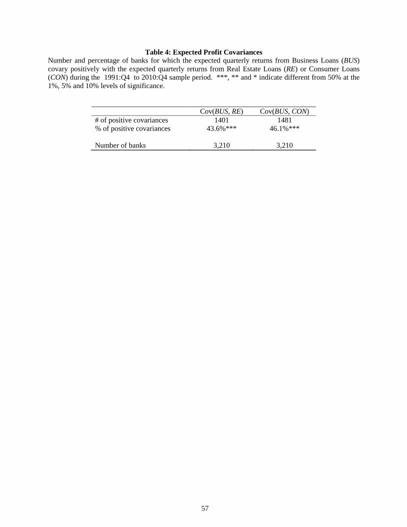
Table 4: Expected Profit Covariances Number and percentage of banks for which the expected quarterly returns from Business Loans (BUS) covary positively with the expected quarterly returns from Real Estate Loans (RE) or Consumer Loans (CON) during the 1991:Q4 to 2010:Q4 sample period. ***, ** and * indicate different from 50% at the 1%, 5% and 10% levels of significance.

Cov(BUS, RE) Cov(BUS, CON) # of positive covariances 1401 1481 % of positive covariances 43.6%*** 46.1%*** Number of banks 3,210 3,210

57

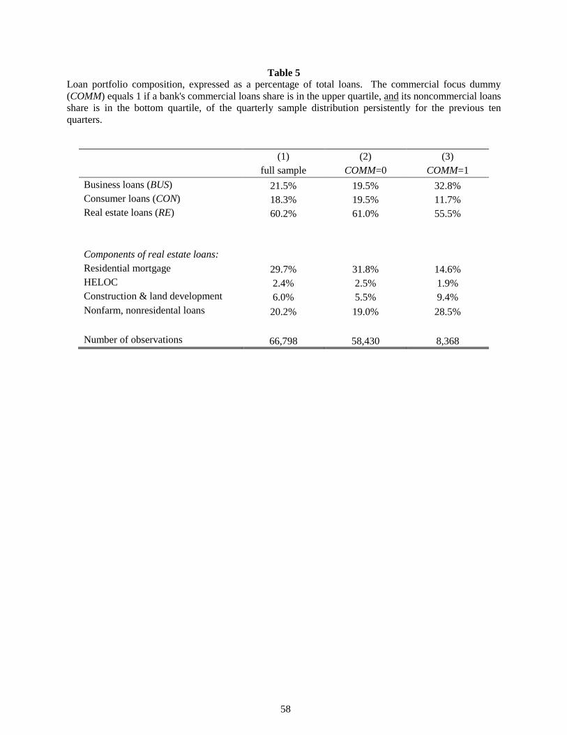
Table 5 Loan portfolio composition, expressed as a percentage of total loans. The commercial focus dummy (COMM) equals 1 if a bank's commercial loans share is in the upper quartile, and its noncommercial loans share is in the bottom quartile, of the quarterly sample distribution persistently for the previous ten quarters.

(1) (2) (3)

full sample COMM=0 COMM=1

Business loans (BUS) 21.5% 19.5% 32.8% Consumer loans (CON) 18.3% 19.5% 11.7% Real estate loans (RE) 60.2% 61.0% 55.5%

Components of real estate loans: Residential mortgage 29.7% 31.8% 14.6% HELOC 2.4% 2.5% 1.9% Construction & land development 6.0% 5.5% 9.4% Nonfarm, nonresidental loans 20.2% 19.0% 28.5% Number of observations 66,798 58,430 8,368

58

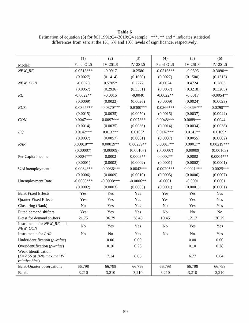
Table 6 Estimation of equation (5) for full 1991:Q4-2010:Q4 sample. ***, ** and * indicates statistical

differences from zero at the 1%, 5% and 10% levels of significance, respectively.

(1) (2) (3) (4) (5) (6)

Model: Panel OLS IV-2SLS IV-2SLS Panel OLS IV-2SLS IV-2SLS NEW_RE -0.0513*** -0.0917 -0.2580 -0.0516*** -0.0895 -0.3090**

(0.0027) (0.1414) (0.1660) (0.0027) (0.1500) (0.1313) NEW_CON -0.0023 0.5705* 0.2277 -0.0024 0.4724 0.2803

(0.0057) (0.2936) (0.3351) (0.0057) (0.3218) (0.3285) RE -0.0022** -0.0015 -0.0040 -0.0022** -0.0017 -0.0054**

(0.0009) (0.0022) (0.0026) (0.0009) (0.0024) (0.0023) BUS -0.0365*** -0.0370*** -0.0300*** -0.0366*** -0.0369*** -0.0290***

(0.0015) (0.0035) (0.0050) (0.0015) (0.0037) (0.0044) CON 0.0047*** 0.0097*** 0.0073** 0.0048*** 0.0089*** 0.0044

(0.0014) (0.0035) (0.0036) (0.0014) (0.0034) (0.0038) EQ 0.0142*** 0.0137** 0.0103* 0.0147*** 0.0141** 0.0109*

(0.0037) (0.0057) (0.0061) (0.0037) (0.0055) (0.0062) RAR 0.00018*** 0.00019** 0.00239** 0.00017** 0.00017* 0.00219*** (0.00007) (0.00009) (0.00107) (0.00007) (0.00009) (0.00103) Per Capita Income 0.0004*** 0.0002 0.0003** 0.0002** 0.0002 0.0004*** (0.0001) (0.0002) (0.0002) (0.0001) (0.0002) (0.0001) %ΔUnemployment -0.0034*** -0.0036*** -0.0042*** -0.0020*** -0.0021*** -0.0025*** (0.0006) (0.0009) (0.0010) (0.0005) (0.0006) (0.0007) Unemployment Rate -0.0008*** -0.0008*** -0.0006** -0.0001 -0.0001 0.0001 (0.0002) (0.0003) (0.0003) (0.0001) (0.0001) (0.0001) Bank Fixed Effects Yes Yes Yes Yes Yes Yes Quarter Fixed Effects Yes Yes Yes Yes Yes Yes Clustering (Bank) No Yes Yes No Yes Yes Fitted demand shifters Yes Yes Yes No No No F-test for demand shifters 21.75 36.79 38.43 10.45 12.17 20.29 Instruments for NEW_RE and NEW_CON No Yes Yes No Yes Yes

Instruments for RAR No No Yes No No Yes Underidentification (p-value) 0.00 0.00 0.00 0.00 Overidentification (p-value) 0.10 0.23 0.10 0.28 Weak Identification (F=7.56 at 10% maximal IV relative bias)

7.14 8.05 6.77 6.64

Bank-Quarter observations 66,798 66,798 66,798 66,798 66,798 66,798 Banks 3,210 3,210 3,210 3,210 3,210 3,210

59

Table 7 Testing for risk overhang effects using exogenous variation in bank organization form and state tax law. SUB_S is a dummy equal to one for banks with subchapter S status. TAXINC is a dummy equal to one during each of the first four quarters following an increase in state personal tax rates in the bank’s home state. The baseline 2SLS-IV model of equation (5) is augmented to include interactions of SUB_S and TAXINC with the main variables of interest as well as a control variable (TAX CHANGE) for changes in state level personal income tax rates. Model is estimated for a subsample of our main database from 1998:Q1 to 2010:Q4. ***,**, and * indicate statistical differences from zero at the 1%, 5%, and 10% levels of significance, respectively.

(1) (2) (3) (4) (5)

Estimated partial derivatives evaluated for different values of the SUB_S and TAXINC dummy variables:

SUB_S = 0 SUB_S = 1 SUB_S = 0 SUB_S = 1

TAXINC = 0 TAXINC = 0 TAXINC = 1 TAXINC = 1 NEW_RE 0.0972 (0.1515) NEW_CON 1.0189** (0.4520) RE 0.0011 0.0011 0.0029 0.0067 0.0305**

(0.0044) (0.0044) (0.0056) (0.0088) (0.0137) RE*SUB_S 0.0018 (0.0038) RE*TAXINC 0.0056 (0.0071) RE*SUB_S*TAXINC 0.0220** (0.0110) BUS -0.0428*** -0.0428*** -0.0717*** -0.0442*** -0.1355***

(0.0062) (0.0062) (0.0071) (0.0136) (0.0253) BUS*SUB_S -0.0289*** (0.0075) BUS*TAXINC -0.0014 (0.0124) BUS*SUB_S*TAXINC -0.0624** (0.0257) CON 0.0204*** 0.0204*** 0.0234* 0.0463** 0.1066**

(0.0078) (0.0078) (0.0137) (0.0193) (0.0511) CON*SUB_S 0.0030 (0.0113) CON*TAXINC 0.0259 (0.0162) CON*SUB_S*TAXINC 0.0573** (0.0286)

60

EQ 0.0240** 0.0240** -0.0040 0.0181 0.0382

(0.0098) (0.0098) (0.0149) (0.0288) (0.0313) EQ*SUB_S -0.0280* (0.0152) EQ*TAXINC -0.0058 (0.0274) EQ*SUB_S*TAXINC 0.0481 (0.0376) RAR 0.00049** 0.00049** 0.00042 0.00065 -0.00011

(0.00024) (0.00024) (0.00032) (0.00044) (0.00092) RAR*SUB_S -0.0001 (0.0002) RAR*TAXINC 0.0002 (0.0004) RAR*SUB_S*TAXINC -0.0007 (0.0009) SUB_S 0.0044* (0.0025) TAXINC -0.0031 (0.0048) TAX CHANGE 0.0453 (0.2892) Bank Fixed Effects Yes Quarter Fixed Effects Yes Clustering (Bank) Yes Fitted demand shifters Yes F-Test for demand shifters 9.40 Instruments for NEW_RE, NEW_CON and RAR Yes

Underidentification (p-value) 0.00 Overidentification (p-value) 0.21 Weak Identification (F=7.56 at 10% level) 7.40 Bank-Quarter Observations 31,380 Banks 1,918

61

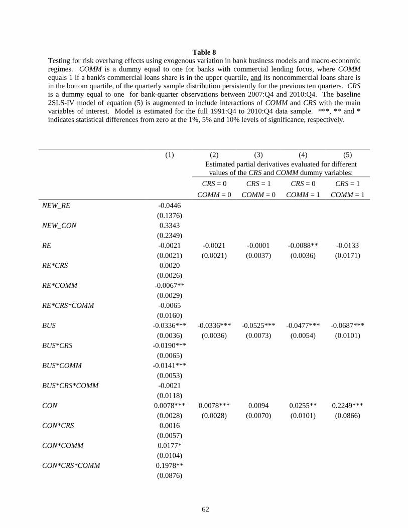
Table 8 Testing for risk overhang effects using exogenous variation in bank business models and macro-economic regimes. COMM is a dummy equal to one for banks with commercial lending focus, where COMM equals 1 if a bank's commercial loans share is in the upper quartile, and its noncommercial loans share is in the bottom quartile, of the quarterly sample distribution persistently for the previous ten quarters. CRS is a dummy equal to one for bank-quarter observations between 2007:Q4 and 2010:Q4. The baseline 2SLS-IV model of equation (5) is augmented to include interactions of COMM and CRS with the main variables of interest. Model is estimated for the full 1991:Q4 to 2010:Q4 data sample. ***, ** and * indicates statistical differences from zero at the 1%, 5% and 10% levels of significance, respectively.

(1) (2) (3) (4) (5)

Estimated partial derivatives evaluated for different values of the CRS and COMM dummy variables:

CRS = 0 CRS = 1 CRS = 0 CRS = 1

COMM = 0 COMM = 0 COMM = 1 COMM = 1 NEW_RE -0.0446

(0.1376) NEW_CON 0.3343

(0.2349)

RE -0.0021 -0.0021 -0.0001 -0.0088** -0.0133

(0.0021) (0.0021) (0.0037) (0.0036) (0.0171)

RE*CRS 0.0020

(0.0026)

RE*COMM -0.0067**

(0.0029)

RE*CRS*COMM -0.0065

(0.0160)

BUS -0.0336*** -0.0336*** -0.0525*** -0.0477*** -0.0687***

(0.0036) (0.0036) (0.0073) (0.0054) (0.0101)

BUS*CRS -0.0190***

(0.0065)

BUS*COMM -0.0141***

(0.0053)

BUS*CRS*COMM -0.0021

(0.0118)

CON 0.0078*** 0.0078*** 0.0094 0.0255** 0.2249***

(0.0028) (0.0028) (0.0070) (0.0101) (0.0866)

CON*CRS 0.0016

(0.0057)

CON*COMM 0.0177*

(0.0104)

CON*CRS*COMM 0.1978**

(0.0876)

62

EQ 0.0080* 0.0080* 0.0213** 0.0494*** 0.1243***

(0.0058) (0.0058) (0.0102) (0.0126) (0.0352)

EQ*CRS 0.0133

(0.0097)

EQ*COMM 0.0414***

(0.0129)

EQ*CRS*COMM 0.0616*

(0.0338)

RAR 0.00042** 0.00042** 0.00028 0.00060*** -0.00480

(0.00021) (0.00021) (0.00030) (0.00021) (0.00294)

RAR*CRS -0.0001

(0.0001)

RAR*COMM 0.0002

(0.0001)

RAR*CRS*COMM -0.0053**

(0.0023)

COMM -0.0012 (0.0017) CRS -0.0031 (0.0021) Bank Fixed Effects Yes Quarter Fixed Effects Yes Clustering (Bank) Yes Fitted demand shifters Yes F-Test for demand shifters 8.36 Instruments for NEW_RE, NEW_CON and RAR Yes

Underidentification (p-value) 0.00 Overidentification (p-value) 0.19 Weak Identification (F=7.56 at 10% maximal IV relative bias) 9.86

∂NEW_BUS/∂CRS(COMM=0) -0.0033** ∂NEW_BUS/∂CRS(COMM=1) 0.0157*** Bank-Quarter Observations 66,798 Banks 3,210

63

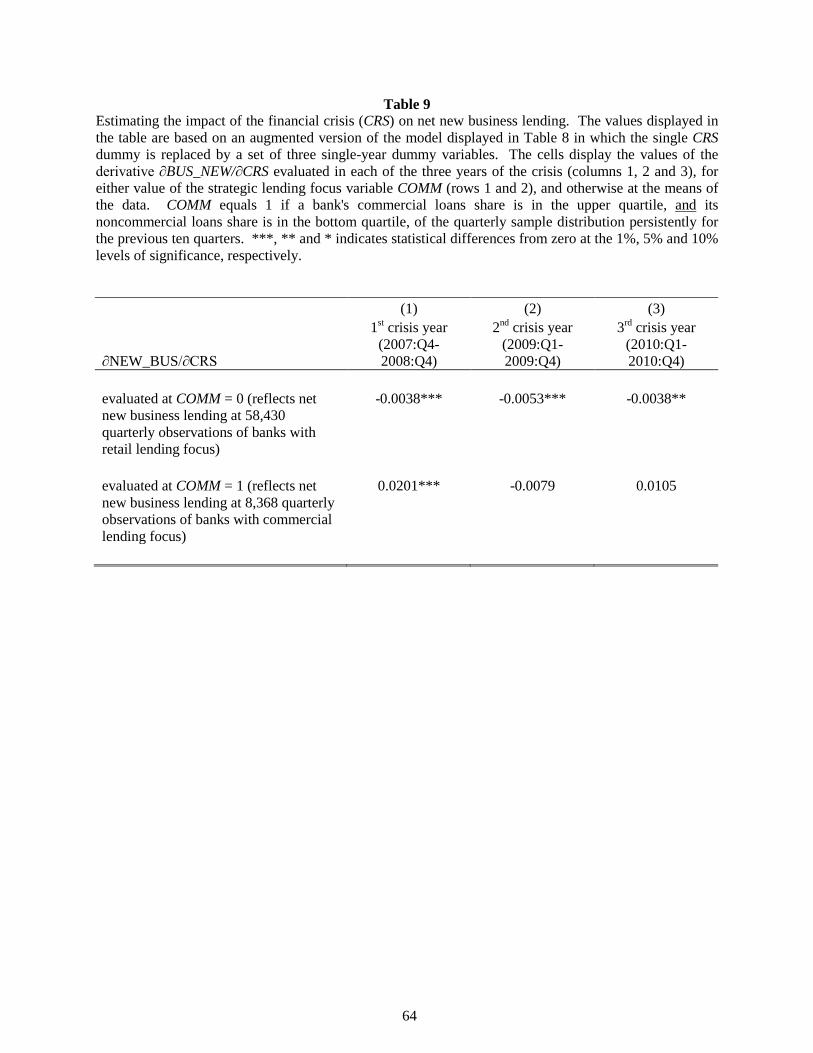
Table 9 Estimating the impact of the financial crisis (CRS) on net new business lending. The values displayed in the table are based on an augmented version of the model displayed in Table 8 in which the single CRS dummy is replaced by a set of three single-year dummy variables. The cells display the values of the derivative ∂BUS_NEW/∂CRS evaluated in each of the three years of the crisis (columns 1, 2 and 3), for either value of the strategic lending focus variable COMM (rows 1 and 2), and otherwise at the means of the data. COMM equals 1 if a bank's commercial loans share is in the upper quartile, and its noncommercial loans share is in the bottom quartile, of the quarterly sample distribution persistently for the previous ten quarters. ***, ** and * indicates statistical differences from zero at the 1%, 5% and 10% levels of significance, respectively.

(1) (2) (3)

∂NEW_BUS/∂CRS

1st crisis year (2007:Q4-2008:Q4)

2nd crisis year (2009:Q1-2009:Q4)

3rd crisis year (2010:Q1-2010:Q4)

evaluated at COMM = 0 (reflects net new business lending at 58,430 quarterly observations of banks with retail lending focus)

-0.0038*** -0.0053*** -0.0038**

evaluated at COMM = 1 (reflects net new business lending at 8,368 quarterly observations of banks with commercial lending focus)

0.0201*** -0.0079 0.0105

64

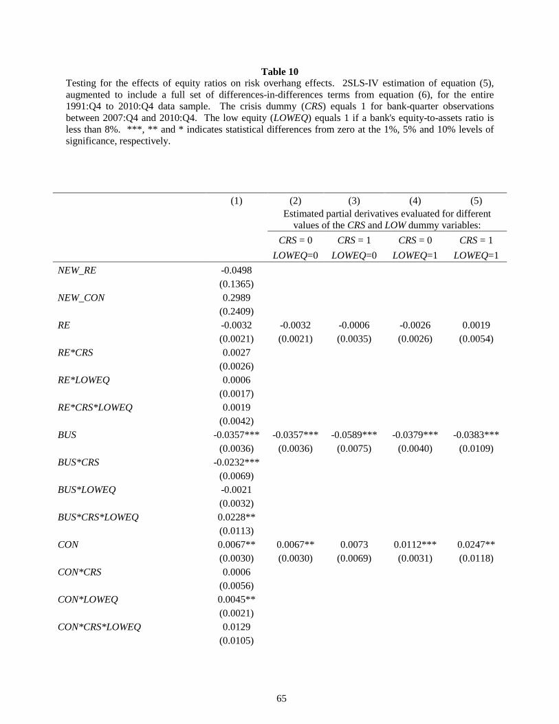
Table 10 Testing for the effects of equity ratios on risk overhang effects. 2SLS-IV estimation of equation (5), augmented to include a full set of differences-in-differences terms from equation (6), for the entire 1991:Q4 to 2010:Q4 data sample. The crisis dummy (CRS) equals 1 for bank-quarter observations between 2007:Q4 and 2010:Q4. The low equity (LOWEQ) equals 1 if a bank's equity-to-assets ratio is less than 8%. ***, ** and * indicates statistical differences from zero at the 1%, 5% and 10% levels of significance, respectively.

(1) (2) (3) (4) (5)

Estimated partial derivatives evaluated for different values of the CRS and LOW dummy variables:

CRS = 0 CRS = 1 CRS = 0 CRS = 1

LOWEQ=0 LOWEQ=0 LOWEQ=1 LOWEQ=1 NEW_RE -0.0498

(0.1365)

NEW_CON 0.2989

(0.2409)

RE -0.0032 -0.0032 -0.0006 -0.0026 0.0019

(0.0021) (0.0021) (0.0035) (0.0026) (0.0054)

RE*CRS 0.0027

(0.0026)

RE*LOWEQ 0.0006

(0.0017)

RE*CRS*LOWEQ 0.0019

(0.0042)

BUS -0.0357*** -0.0357*** -0.0589*** -0.0379*** -0.0383***

(0.0036) (0.0036) (0.0075) (0.0040) (0.0109)

BUS*CRS -0.0232***

(0.0069)

BUS*LOWEQ -0.0021

(0.0032)

BUS*CRS*LOWEQ 0.0228**

(0.0113)

CON 0.0067** 0.0067** 0.0073 0.0112*** 0.0247**

(0.0030) (0.0030) (0.0069) (0.0031) (0.0118)

CON*CRS 0.0006

(0.0056)

CON*LOWEQ 0.0045**

(0.0021)

CON*CRS*LOWEQ 0.0129

(0.0105)

65

EQ 0.0093 0.0093 0.0269** 0.0812*** 0.0276

(0.0063) (0.0063) (0.0115) (0.0187) (0.0491)

EQ*CRS 0.0176*

(0.0103)

EQ*LOWEQ 0.0719***

(0.0202)

EQ*CRS*LOWEQ -0.0712*

(0.0429)

RAR 0.00037* 0.00037* 0.00010 0.00048*** 0.00071

(0.00021) (0.00021) (0.00031) (0.00020) (0.00070)

RAR*CRS -0.0003

(0.0002)

RAR*LOWEQ 0.0001

(0.0001)

RAR*CRS*LOWEQ 0.0005

(0.0007)

LOWEQ -0.0057*** (0.0016) CRS -0.0030 (-0.0021) Bank Fixed Effects Yes Quarter Fixed Effects Yes Clustering (Bank) Yes Fitted demand shifters Yes F-Test for demand shifters 9.24 Instruments for NEW_RE, NEW_CON and RAR Yes

Underidentification (p-value) 0.00 Overidentification (p-value) 0.29 Weak Identification (F=7.56 at 10% level) 9.99 ∂NEW_BUS/∂CRS(LOWEQ=0) -0.0033** ∂NEW_BUS/∂CRS(LOWEQ=1) -0.0049** Bank-Quarter Observations 66,798 Banks 3,210

66

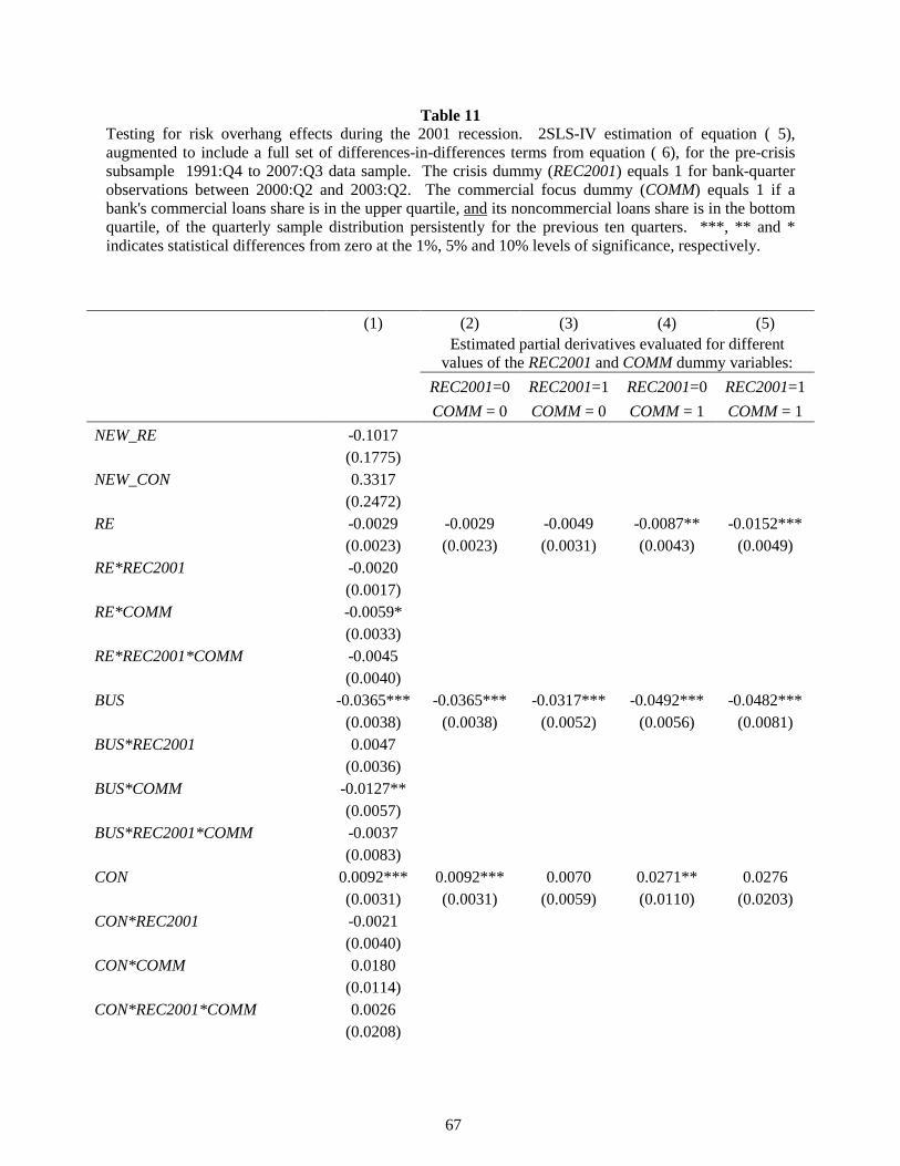
Table 11 Testing for risk overhang effects during the 2001 recession. 2SLS-IV estimation of equation ( 5), augmented to include a full set of differences-in-differences terms from equation ( 6), for the pre-crisis subsample 1991:Q4 to 2007:Q3 data sample. The crisis dummy (REC2001) equals 1 for bank-quarter observations between 2000:Q2 and 2003:Q2. The commercial focus dummy (COMM) equals 1 if a bank's commercial loans share is in the upper quartile, and its noncommercial loans share is in the bottom quartile, of the quarterly sample distribution persistently for the previous ten quarters. ***, ** and * indicates statistical differences from zero at the 1%, 5% and 10% levels of significance, respectively.

(1) (2) (3) (4) (5)

Estimated partial derivatives evaluated for different values of the REC2001 and COMM dummy variables:

REC2001=0 REC2001=1 REC2001=0 REC2001=1

COMM = 0 COMM = 0 COMM = 1 COMM = 1 NEW_RE -0.1017

(0.1775) NEW_CON 0.3317

(0.2472)

RE -0.0029 -0.0029 -0.0049 -0.0087** -0.0152***

(0.0023) (0.0023) (0.0031) (0.0043) (0.0049)

RE*REC2001 -0.0020

(0.0017)

RE*COMM -0.0059*

(0.0033)

RE*REC2001*COMM -0.0045

(0.0040)

BUS -0.0365*** -0.0365*** -0.0317*** -0.0492*** -0.0482***

(0.0038) (0.0038) (0.0052) (0.0056) (0.0081)

BUS*REC2001 0.0047

(0.0036)

BUS*COMM -0.0127**

(0.0057)

BUS*REC2001*COMM -0.0037

(0.0083)

CON 0.0092*** 0.0092*** 0.0070 0.0271** 0.0276

(0.0031) (0.0031) (0.0059) (0.0110) (0.0203)

CON*REC2001 -0.0021

(0.0040)

CON*COMM 0.0180

(0.0114)

CON*REC2001*COMM 0.0026

(0.0208)

67

EQ 0.0100 0.0100 -0.0011 0.0494*** 0.0461***

(0.0063) (0.0063) (0.0083) (0.0135) (0.0159)

EQ*REC2001 -0.0110

(0.0084)

EQ*COMM 0.0395***

(0.0137)

EQ*REC2001*COMM 0.0076

(0.0152)

RAR 0.00043** 0.00043** 0.00028 0.00057** 0.00084***

(0.00022) (0.00022) (0.00024) (0.00023) (0.00032)

RAR*REC2001 -0.0001

(0.0001)

RAR*COMM 0.0001

(0.0001)

RAR*REC2001*COMM 0.0004

(0.0003)

COMM -0.0015 (0.0018) REC2001 0.0024

(0.0015) Bank Fixed Effects Yes

Quarter Fixed Effects Yes Clustering (Bank) Yes Fitted demand shifters Yes F-Test for demand shifters 7.57 Instruments for NEW_RE, NEW_CON and RAR Yes

Underidentification (p-value) 0.00 Overidentification (p-value) 0.49 Weak Identification (F=7.56 at 10% level) 8.41 ∂NEW_BUS/∂CRS(COMM=0) -0.0002 ∂NEW_BUS/∂CRS(COMM=1) 0.0001 Bank-Quarter Observations 63,313 Banks 3,192

68

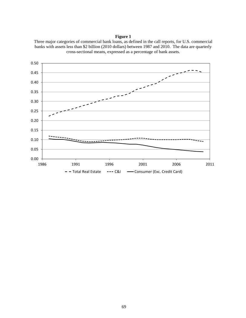
Figure 1

Three major categories of commercial bank loans, as defined in the call reports, for U.S. commercial banks with assets less than $2 billion (2010 dollars) between 1987 and 2010. The data are quarterly

cross-sectional means, expressed as a percentage of bank assets.

0.00

0.05

0.10

0.15

0.20

0.25

0.30

0.35

0.40

0.45

0.50

1986 1991 1996 2001 2006 2011

Total Real Estate C&I Consumer (Exc. Credit Card)

69

Figure 2

Kaplan-Meier estimates. Hazard probability that a commercial focus bank (COM=1) will abandon its strategy after having practiced it for a given number of consecutive quarters (horizontal axis).

0.00

0.01

0.02

0.03

0.04

0.05

0.06

0.07

0.08

0.09

0.10

0.11

0.12

1 3 5 7 9 11 13 15 17 19 21 23 25 27 30 32 34 37 42 45 51 53 65Quarters

70

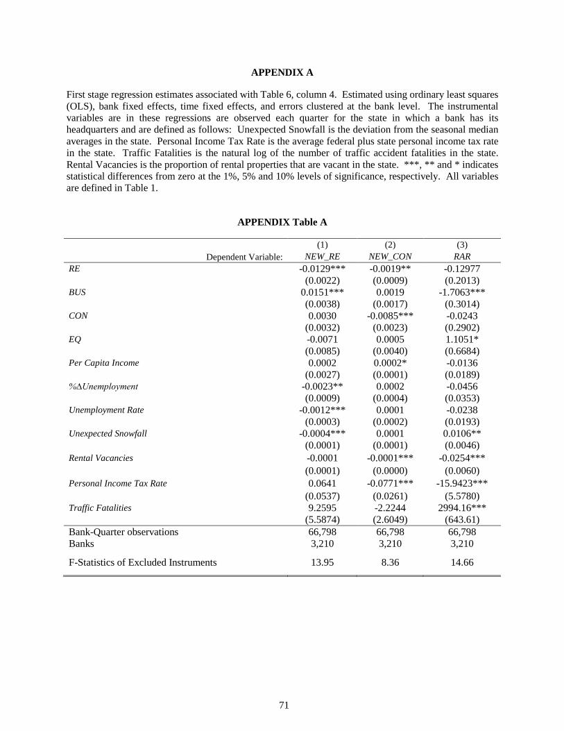
APPENDIX A First stage regression estimates associated with Table 6, column 4. Estimated using ordinary least squares (OLS), bank fixed effects, time fixed effects, and errors clustered at the bank level. The instrumental variables are in these regressions are observed each quarter for the state in which a bank has its headquarters and are defined as follows: Unexpected Snowfall is the deviation from the seasonal median averages in the state. Personal Income Tax Rate is the average federal plus state personal income tax rate in the state. Traffic Fatalities is the natural log of the number of traffic accident fatalities in the state. Rental Vacancies is the proportion of rental properties that are vacant in the state. ***, ** and * indicates statistical differences from zero at the 1%, 5% and 10% levels of significance, respectively. All variables are defined in Table 1.

APPENDIX Table A (1) (2) (3)

Dependent Variable: NEW_RE NEW_CON RAR RE -0.0129*** -0.0019** -0.12977 (0.0022) (0.0009) (0.2013) BUS 0.0151*** 0.0019 -1.7063*** (0.0038) (0.0017) (0.3014) CON 0.0030 -0.0085*** -0.0243 (0.0032) (0.0023) (0.2902) EQ -0.0071 0.0005 1.1051* (0.0085) (0.0040) (0.6684) Per Capita Income 0.0002 0.0002* -0.0136 (0.0027) (0.0001) (0.0189) %∆Unemployment -0.0023** 0.0002 -0.0456 (0.0009) (0.0004) (0.0353) Unemployment Rate -0.0012*** 0.0001 -0.0238 (0.0003) (0.0002) (0.0193) Unexpected Snowfall -0.0004*** 0.0001 0.0106** (0.0001) (0.0001) (0.0046) Rental Vacancies -0.0001 -0.0001*** -0.0254*** (0.0001) (0.0000) (0.0060) Personal Income Tax Rate 0.0641 -0.0771*** -15.9423*** (0.0537) (0.0261) (5.5780) Traffic Fatalities 9.2595 -2.2244 2994.16*** (5.5874) (2.6049) (643.61) Bank-Quarter observations 66,798 66,798 66,798 Banks 3,210 3,210 3,210

F-Statistics of Excluded Instruments 13.95 8.36 14.66

71

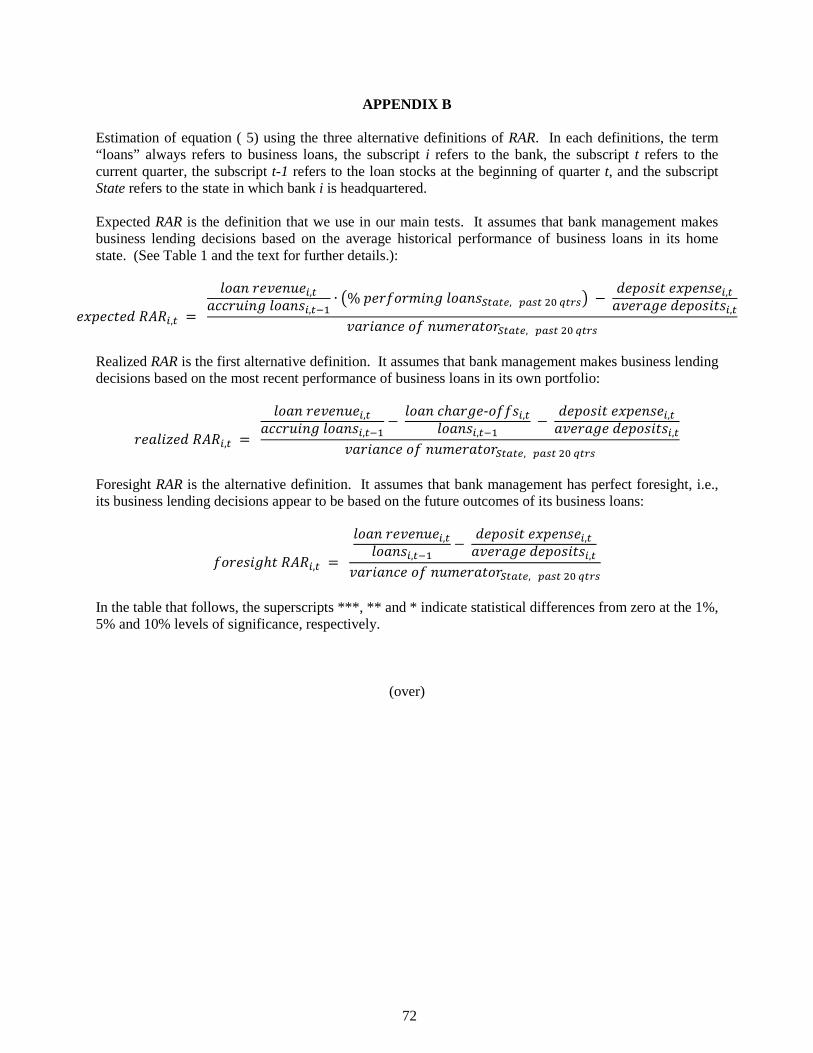
APPENDIX B Estimation of equation ( 5) using the three alternative definitions of RAR. In each definitions, the term “loans” always refers to business loans, the subscript i refers to the bank, the subscript t refers to the current quarter, the subscript t-1 refers to the loan stocks at the beginning of quarter t, and the subscript State refers to the state in which bank i is headquartered. Expected RAR is the definition that we use in our main tests. It assumes that bank management makes business lending decisions based on the average historical performance of business loans in its home state. (See Table 1 and the text for further details.):

𝑒𝑥𝑝𝑒𝑐𝑡𝑒𝑑 𝑅𝐴𝑅𝑖,𝑡 =

𝑙𝑜𝑎𝑛 𝑟𝑒𝑣𝑒𝑛𝑢𝑒𝑖,𝑡𝑎𝑐𝑐𝑟𝑢𝑖𝑛𝑔 𝑙𝑜𝑎𝑛𝑠𝑖,𝑡−1

∙ �% 𝑝𝑒𝑟𝑓𝑜𝑟𝑚𝑖𝑛𝑔 𝑙𝑜𝑎𝑛𝑠𝑆𝑡𝑎𝑡𝑒, 𝑝𝑎𝑠𝑡 20 𝑞𝑡𝑟𝑠� − 𝑑𝑒𝑝𝑜𝑠𝑖𝑡 𝑒𝑥𝑝𝑒𝑛𝑠𝑒𝑖,𝑡𝑎𝑣𝑒𝑟𝑎𝑔𝑒 𝑑𝑒𝑝𝑜𝑠𝑖𝑡𝑠𝑖,𝑡

𝑣𝑎𝑟𝑖𝑎𝑛𝑐𝑒 𝑜𝑓 𝑛𝑢𝑚𝑒𝑟𝑎𝑡𝑜𝑟𝑆𝑡𝑎𝑡𝑒, 𝑝𝑎𝑠𝑡 20 𝑞𝑡𝑟𝑠

Realized RAR is the first alternative definition. It assumes that bank management makes business lending decisions based on the most recent performance of business loans in its own portfolio:

𝑟𝑒𝑎𝑙𝑖𝑧𝑒𝑑 𝑅𝐴𝑅𝑖,𝑡 =

𝑙𝑜𝑎𝑛 𝑟𝑒𝑣𝑒𝑛𝑢𝑒𝑖,𝑡𝑎𝑐𝑐𝑟𝑢𝑖𝑛𝑔 𝑙𝑜𝑎𝑛𝑠𝑖,𝑡−1

− 𝑙𝑜𝑎𝑛 𝑐ℎ𝑎𝑟𝑔𝑒-𝑜𝑓𝑓𝑠𝑖,𝑡

𝑙𝑜𝑎𝑛𝑠𝑖,𝑡−1 −

𝑑𝑒𝑝𝑜𝑠𝑖𝑡 𝑒𝑥𝑝𝑒𝑛𝑠𝑒𝑖,𝑡𝑎𝑣𝑒𝑟𝑎𝑔𝑒 𝑑𝑒𝑝𝑜𝑠𝑖𝑡𝑠𝑖,𝑡

𝑣𝑎𝑟𝑖𝑎𝑛𝑐𝑒 𝑜𝑓 𝑛𝑢𝑚𝑒𝑟𝑎𝑡𝑜𝑟𝑆𝑡𝑎𝑡𝑒, 𝑝𝑎𝑠𝑡 20 𝑞𝑡𝑟𝑠

Foresight RAR is the alternative definition. It assumes that bank management has perfect foresight, i.e., its business lending decisions appear to be based on the future outcomes of its business loans:

𝑓𝑜𝑟𝑒𝑠𝑖𝑔ℎ𝑡 𝑅𝐴𝑅𝑖,𝑡 =

𝑙𝑜𝑎𝑛 𝑟𝑒𝑣𝑒𝑛𝑢𝑒𝑖,𝑡𝑙𝑜𝑎𝑛𝑠𝑖,𝑡−1

− 𝑑𝑒𝑝𝑜𝑠𝑖𝑡 𝑒𝑥𝑝𝑒𝑛𝑠𝑒𝑖,𝑡𝑎𝑣𝑒𝑟𝑎𝑔𝑒 𝑑𝑒𝑝𝑜𝑠𝑖𝑡𝑠𝑖,𝑡

𝑣𝑎𝑟𝑖𝑎𝑛𝑐𝑒 𝑜𝑓 𝑛𝑢𝑚𝑒𝑟𝑎𝑡𝑜𝑟𝑆𝑡𝑎𝑡𝑒, 𝑝𝑎𝑠𝑡 20 𝑞𝑡𝑟𝑠

In the table that follows, the superscripts ***, ** and * indicate statistical differences from zero at the 1%, 5% and 10% levels of significance, respectively.

(over)

72

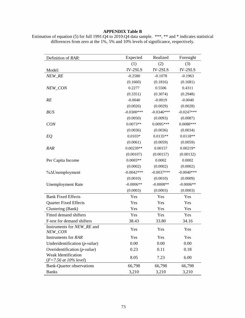
APPENDIX Table B Estimation of equation (5) for full 1991:Q4 to 2010:Q4 data sample. ***, ** and * indicates statistical

differences from zero at the 1%, 5% and 10% levels of significance, respectively.

Definition of RAR: Expected Realized Foresight (1) (2) (3) Model: IV-2SLS IV-2SLS IV-2SLS NEW_RE -0.2580 -0.1078 -0.1963

(0.1660) (0.1816) (0.1681) NEW_CON 0.2277 0.5506 0.4311

(0.3351) (0.3074) (0.2948) RE -0.0040 -0.0019 -0.0040

(0.0026) (0.0029) (0.0028) BUS -0.0300*** -0.0346*** -0.0247***

(0.0050) (0.0093) (0.0087) CON 0.0073** 0.0095*** 0.0088***

(0.0036) (0.0036) (0.0034) EQ 0.0103* 0.0135** 0.0118**

(0.0061) (0.0059) (0.0059) RAR 0.00239** 0.00157 0.00219* (0.00107) (0.00157) (0.00132) Per Capita Income 0.0003** 0.0002 0.0002 (0.0002) (0.0002) (0.0002) %ΔUnemployment -0.0042*** -0.0037*** -0.0040*** (0.0010) (0.0010) (0.0009) Unemployment Rate -0.0006** -0.0008** -0.0006** (0.0003) (0.0003) (0.0003) Bank Fixed Effects Yes Yes Yes Quarter Fixed Effects Yes Yes Yes Clustering (Bank) Yes Yes Yes Fitted demand shifters Yes Yes Yes F-test for demand shifters 38.43 33.80 34.16 Instruments for NEW_RE and NEW_CON Yes Yes Yes

Instruments for RAR Yes Yes Yes Underidentification (p-value) 0.00 0.00 0.00 Overidentification (p-value) 0.23 0.11 0.18 Weak Identification (F=7.56 at 10% level) 8.05 7.23 6.00

Bank-Quarter observations 66,798 66,798 66,798 Banks 3,210 3,210 3,210

73