risk management series -...

RiskManagementSeries

AAAAAAAAAAAAAAAAAAAAAAAAAAAAAAAAAAAAAAAA





































AAAAAAAAAAAAAAAAAAAAAAAAAAAAAA

January 1996 Managing MarketExposure

Robert LittermanKurt Winkelmann


Acknowledgements The authors are grateful to Mike Asay, Alex Bergier, Jean-

Robert Litterman is a Partner in Firmwide Risk at Gold-man, Sachs & Co. in New York. Kurt Winkelmann is anExecutive Director in Fixed Income Research at GoldmanSachs International in London.

Editor: Ronald A. Krieger

Copyright © 1996 by Goldman, Sachs & Co.

This material is for your private information, and we are not soliciting any actionbased upon it. Certain transactions, including those involving futures, options, andhigh yield securities, give rise to substantial risk and are not suitable for all inves-tors. Opinions expressed are our present opinions only. The material is based uponinformation that we consider reliable, but we do not represent that it is accurate orcomplete, and it should not be relied upon as such. We, or persons involved in thepreparation or issuance of this material, may from time to time have long or shortpositions in, and buy or sell, securities, futures, or options identical with or relatedto those mentioned herein. This material has been issued by Goldman, Sachs & Co.and has been approved by Goldman Sachs International, a member of The Securi-ties and Futures Authority, in connection with its distribution in the UnitedKingdom, and by Goldman Sachs Canada in connection with its distribution inCanada. Further information on any of the securities, futures, or options mentionedin this material may be obtained upon request. For this purpose, persons in Italyshould contact Goldman Sachs S.I.M. S.p.A. in Milan, or at its London branch officeat 133 Fleet Street. Goldman Sachs International may have acted upon or used thisresearch prior to or immediately following its publication.

Paul Calamaro, Tom Macirowski, Scott Pinkus, and KenSingleton for their helpful suggestions. We owe specialthanks to Ugo Loser for his help in developing the ideas forusing Market Exposure in bond trading. We are also indebt-ed to the late Fischer Black for his incisive comments on anearlier draft of this report, as well as for his continuingintellectual support and unfailing wisdom over many yearsof fruitful collaboration.

Robert LittermanNew York212-902-1677

Kurt WinkelmannLondon44-171-774-5545


Managing Market Exposure

Contents

Executive Summary

I. Introduction . . . . . . . . . . . . . . . . . . . . . . . . . . . 1

II. Risk Factors, Benchmarks, andMarket Exposure . . . . . . . . . . . . . . . . . . . . . . . 3Market Exposure of a Global Portfolio . . . . . . . . . 5Market Factors vs. Residual Factors . . . . . . . . . . 6The Relevant `Market' . . . . . . . . . . . . . . . . . . . . 7

How Goldman Sachs Uses Market Exposurein Monitoring Its Bond Trading Risk . . . . . . . . . 9

III. Market Exposure and the GlobalBond Fund Manager . . . . . . . . . . . . . . . . . . . 10Market Exposure and Portfolio Performance . . . 11Residual Risk and Portfolio Performance . . . . . . 18

IV. Market Exposure and the GlobalBond Trader . . . . . . . . . . . . . . . . . . . . . . . . . . 20Creating `Market-Neutral' Weights forRelative Value Trades . . . . . . . . . . . . . . . . . . . . 21Alternative Approaches . . . . . . . . . . . . . . . . . . . 24

V. Summary and Conclusions . . . . . . . . . . . . . . 27

Appendix A. Optimal PortfolioConstraints and Weights . . . . . . . . . 28

Appendix B. The Mapping Between Viewsand Portfolio Weights . . . . . . . . . . . . 31


Executive Summary In this paper, we introduce a new method for measuring andcontrolling a portfolio's market risk. We call this measure a port-folio's Market Exposure, which we compute by explicitly accountingfor the volatilities and correlations of different assets. We arguethat computing a portfolio's Market Exposure in this way providesthe best answer to the central question that a fund manager (ortrader) faces: “How is my portfolio likely to perform if the marketrallies?”

Our starting point in this report is a discussion of risk factors andMarket Exposure. Under ideal circumstances, a portfolio's risk(and a benchmark portfolio's risk) can be described in terms ofexposures to “risk factors.” Identification and interpretation ofthese risk factors can often be difficult. Nonetheless, in manysituations, the most important risk factor to control is the MarketExposure — that is, the exposure of the manager's (or trader's)portfolio to the overall market. And for that purpose, all that is re-quired is the set of covariances between the assets in the inves-tor's portfolio and those in the market portfolio.

After discussing risk factors and market risk, we proceed to applyour measure of Market Exposure to the problem faced by a globalbond fund manager. We contrast our measure of Market Exposurewith the usual alternative measure of market risk in a bond port-folio — duration — and show how the assumptions required to useduration correctly are typically violated in practice. We then pro-vide an example that shows how a manager's market risk is bettercontrolled using our measure of Market Exposure.

Finally, we discuss the problem a bond trader faces in the contextof choosing weights for a relative value trade. Usually, tradersattempt to establish weights in a relative value trade in order tobe neutral with respect to market moves. We develop an a priorimeasure of market neutrality (by using a portfolio's implied viewon the market's excess return) and show how our measure ofMarket Exposure can be used to generate market-neutral tradeweights. We then compare our approach to creating market-neutral trades with other methods for calculating trade weights.


Managing Market Exposure

I. Introduction or most investment managers, the fundamental portfo-Flio management problem is to select a portfolio of as-sets that outperforms their benchmark. This problem is

neutral with respect to the choice of benchmark: The bench-mark can be a liability stream (e.g., for a pension fund man-ager), a performance index (e.g., for an investment plan coun-selor) or cash (e.g., for a trader). Naturally, solutions to thisproblem depend on security valuation. However, solving thisproblem also requires a robust risk management framework.

Two developments have increased the complexity of riskmanagement for many investors in recent years. First, in-vestors have greatly expanded their purchases of non-domestic securities. Second, many investors have expandedtheir use of derivatives. Both of these activities have ex-posed investors to risks with which they have had littleprevious experience. Investors have thus become increasing-ly concerned with understanding their global market expo-sures and managing unfamiliar combinations of risk.

Unfortunately, the development of risk management toolshas not kept pace with these investment trends. It is becom-ing harder for investors to answer the question: How muchrisk does my portfolio have relative to my benchmark? Thispaper introduces a new risk management tool that we havedeveloped at Goldman Sachs to help manage our own portfo-lios, as well as to help our customers manage theirs. We callthis tool the Market Exposure. In this paper, we show thatthis simple concept can be very useful for understanding andmanaging global portfolio risk. Indeed, it plays the same rolefor global and multi-asset portfolios that duration and betahave historically played for domestic fixed income and equi-ty portfolios.1

Intuitively, a portfolio's Market Exposure measures its sensi-tivity to market moves. Strictly speaking, the definition ofMarket Exposure is the coefficient in a regression of the

1 While market participants often speak of “market exposure” in a gener-

al sense when discussing risk, we use the term Market Exposure inthis paper in the precise sense of our statistical measure of risk.

5


return of a portfolio on the return of the market.2 The defi-nition of the “market” is not really the issue and can beadjusted as different contexts might warrant.3 For mostinvestors, the market should represent the normal mix ofsecurities that he invests in. For example, for a domesticequity investor, the market should refer to the domesticequity market. In this case, the Market Exposure is exactlythe usual definition of the market beta. Alternatively, for adomestic fixed income investor, the market might refer toone of the standard domestic fixed income indexes. For thiscase, the Market Exposure roughly corresponds to the ratioof the duration of the investor's portfolio to that of thebenchmark (adjusted for the relative yield volatilities).

In the domestic portfolio management examples mentionedabove, Market Exposure corresponds to familiar risk mea-sures. However, determining Market Exposure becomesmore important, and more difficult, in the global context inwhich investors increasingly find themselves. For example,the best measure of the market for a global bond manager isa global bond index. In this case, the manager's MarketExposure is a coefficient that relates the returns on hisportfolio to those of the global bond index and provides ananswer to the most important question an investor faces: “Ifthe market that I invest in goes up, am I likely to outper-form my index?” As we will show below, the usual approachto this question, which is to compare portfolio and indexdurations, can be very misleading in the global context.

Not all investors compare their performance against that ofan index. Hedge fund managers or Goldman Sachs traders,for example, usually try to maximize their returns and mini-mize risk in an absolute sense. In other words, their bench-mark is cash. Such investors may use currencies, commodi-ties, bonds, and equities as asset classes. For investors with

2 The regression coefficient, in this simple context, is the covariance of

these returns divided by the variance of the market return.

3 In particular, we do not require that the “market” in our definition ofMarket Exposure refer to the market portfolio that plays a central rolein the Capital Asset Pricing Model. While that is the most naturalMarket Exposure for the individual investor to be concerned about fromthe perspective of economic theory (since that is the exposure for whicha risk premium should be paid), most investment managers are morenarrowly focused on a particular class of assets.

6


such portfolio management objectives, there is no obviouschoice of the “market.” Nonetheless, the concept of MarketExposure may still be useful. For example, a trader maywell have a portfolio with long and short positions in manysectors of the world's fixed income markets. This trader maywant to know whether the portfolio will make money if allfixed income markets rally. The usual approach is to sumthe durations. But as we will argue in this report, such acalculation can give a very misleading answer. A betterapproach is to calculate the Market Exposure of the posi-tions to an appropriately weighted “global fixed income mar-ket.” In Section III, we provide an example of how this canbe done.

Similarly, a currency trader may want to measure exposureto a dollar rally. A better measure than simply summinglong and short positions in foreign currencies is to measureexposure to a market defined as a set of appropriate weightsin foreign currencies. By predefining a set of such “markets,”a trader can quickly and easily monitor his net long andshort exposures to a wide variety of risks.

In the next section of this report, we discuss the relationshipbetween risk factors, benchmarks, and Market Exposure.Then, in Section III, we examine Market Exposure in thecontext of a portfolio manager measured against a perfor-mance index. Section III also contrasts Market Exposurewith more traditional risk management tools and providesexamples of how Market Exposure improves risk manage-ment. In Section IV, we apply Market Exposure to the riskmanagement problem of traders or hedge fund managers.Finally, Section V summarizes the discussion and providesa brief concluding comment.

II. Risk Factors,Benchmarks, andMarket Exposure

ntuitively, most portfolio managers think about asset re-Iturns in terms of exposure to risk factors that are eitherunderlying fundamentals or related to underlying funda-

mentals. For example, an equity manager might considerindustry classification as an important determinant of equi-ty returns. In general, sources of value are also sources ofrisk; for this manager, therefore, the exposure to differentindustries is a factor that will affect the portfolio's risk.

7


Alternatively, a U.S. fixed income portfolio manager mayregard credit ratings as an important characteristic influenc-ing bond returns. For this manager, exposures to differentcredit ratings become an important determinant of portfolioperformance and risk.

Similarly, a U.S. fixed income manager may treat bondreturns as dependent on three term structure factors — thelevel, slope, and curvature of the yield curve — that explainvirtually all the returns in the U.S. Treasury market. Thesethree risk factors, then, determine the performance of theportfolio relative to the benchmark. In this context, as withthe previous examples, it is natural to think about portfoliostrategies that might trade off exposures to one risk factoragainst another. For example, the portfolio might have 90%of its risk come from being overexposed to one term struc-ture factor: “level.” Or — holding the risk fixed relative toits benchmark — we could restructure the portfolio to focusthe risk on the “slope” factor or on the “curvature” factor.

This approach of defining risk factors is especially useful forcategorizing the types of positions the manager is taking. Inthe examples discussed above, the manager finds his port-folio's risk relative to the benchmark by looking at the expo-sures to the risk factors. We can attribute any volatility ofthe performance in the portfolio relative to the benchmark todifferences in exposures to risk factors plus a residual that,if this approach is to be useful, should be relatively small.

Of course, the risk factors described in the examples abovehave the advantage of being easy to identify. Consequently,it is usually relatively straightforward to structure portfolioswith the desired factor exposure. However, portfolio manage-ment and risk measurement become more problematic inportfolios of global assets, where there are many more fac-tors affecting return, and the factors are more complex andthus not easy to describe or measure. Nonetheless, there arecertain basic exposures that most managers need to under-stand. In particular, almost every manager wants to knowthe answer to the question, “If the market rallies, will Ioutperform my benchmark?” Put differently, a managerwants to know his portfolio's Market Exposure.

8


Market Exposure ofa Global Portfolio

Let's consider a global bond portfolio. Clearly, this portfolio'sperformance and volatility are affected by the level anddirection of changes in interest rates for each country in theportfolio. Suppose for the moment that we are in the sim-plest of all worlds, and that all interest rates move together.In this case, the portfolio's performance is affected not bythe levels and changes in interest rates in each country butrather by a common factor called, perhaps, the “global inter-est rate factor.” Consequently, a portfolio's risk relative toanother portfolio (or benchmark) could be measured in termsof its relative sensitivity to the global interest rate factor,that is, its relative duration. In this simple context, a port-folio's Market Exposure relative to a global benchmark ismerely the ratio of the portfolio's duration to that of thebenchmark. A portfolio is more exposed to the global interestrate factor if it has a longer duration than the benchmark.In this case, if the global interest rate factor rallies, theportfolio will outperform the benchmark, and vice versa.

The real world is not so simple. Interest rates do not allmove together, and the total duration of a global portfoliowill probably not be a good proxy for its Market Exposure.Consider a slightly more complicated and realistic view ofthe global fixed income markets: Suppose that global inter-est rate movements can be described in terms of three sepa-rate blocs, and that interest rate movements are perfectlycorrelated within each bloc and completely uncorrelatedamong the blocs. One such bloc could be a “Europe” bloc,while a second bloc could be a “dollar” bloc, and a third bloccould be a “Japan” bloc. In this case, the blocs themselvesconstitute separate “factors” (e.g., a “Europe” factor). Wemeasure one portfolio's risk relative to another portfolio (orbenchmark) in terms of exposures to the blocs.

For example, suppose that the Europe factor is more volatilethan the dollar or Japan factors, and that the portfolio isoverweighted in the Europe bloc and underweighted in thedollar bloc, relative to the benchmark weights. Since theEurope factor is more volatile and the dollar factor is lessvolatile, and since all three factors are uncorrelated, theportfolio's returns are more volatile than those of the bench-mark. Furthermore, we can describe the volatility of theportfolio's performance relative to that of the benchmark interms of the relative exposures to the Europe, dollar, andJapan factors. Finally, since the factors are uncorrelated, we

9


can describe the portfolio's Market Exposure as a linearcombination of the factor volatilities, with the consequencethat higher exposure to the more volatile Europe factorleads to more Market Exposure. If, on the other hand, thedollar block is more volatile, then the Market Exposure of aportfolio overweighted in the Europe bloc will be lower thanthat of the benchmark.

Consider the two examples of this section. In both cases, westarted with an assumption about the structure of the un-derlying sources of risk. We then used this structure todescribe the correlation between asset returns. The finalstep was to show that the Market Exposure was a functionof the relative exposures to the risk factors. Some readersfamiliar with equity valuation theories may recognize thistype of distinction between risk factors and Market Expo-sure in the context of equity portfolios, where the risk factorapproach forms the basis for the Arbitrage Pricing Theorywhile the Market Exposure approach is the basis for theCapital Asset Pricing Model.

Market Factors vs.Residual Factors

In the real world, unfortunately, trying to identify sources ofrisk by uncovering a set of “factors” from an actual covari-ance matrix of asset returns is a very complicated process,particularly in the context of global fixed income securities.For instance, instability in the correlation matrix of assetreturns suggests that identification of factors is time-depen-dent. Moreover, even if we can isolate factors, finding aneconomic interpretation for these factors is difficult.

However, even though a stable set of “factors” cannot easilybe identified, we can obtain a very natural and useful de-composition of risk of a portfolio by measuring (1) the expo-sure of a portfolio to the risk factors that affect the overallmarket, versus (2) the “residual” exposure to factors thataffect the performance of the portfolio but do not affect thereturns of the market.

In this approach, we avoid the difficult and unnecessary stepof trying to decompose the covariance structure of returnsinto underlying risk factors. Rather, we directly quantify theexposure of a portfolio to the market risk factors.

10


Measuring a portfolio's market risk is fundamentally a fore-casting problem. Consequently, several trade-offs arise indeveloping market risk measures. We would like measuresthat are easy to understand but that simultaneously encom-pass exposure to all risk factors. Since our measure of Mar-ket Exposure is statistical in nature, it provides a moreaccurate, though more complex, answer than accountingmeasures (such as duration) to the forecasting problem,“How is my portfolio likely to perform when the marketrallies?” While our measure does not mitigate the estimationissues surrounding time-varying correlations (and volatili-ties), it has the virtue of being more easily interpreted thanmore-complicated multifactor models.

The Relevant `Market' In general, no single definition of the “market” portfolio willsuffice. For the purpose of understanding risks, most invest-ment managers will want to focus on a capitalization-weighted portfolio that includes securities in which theytransact. A fixed income manager is likely to care about hisexposure to the fixed income markets but not about hisexposure to the equity market. In such a context, the mana-ger's benchmark is likely to be a good proxy for the relevantsubcomponent of the market portfolio.

More generally, however, a diversified investor will careabout exposures to a broad aggregation of asset classes.Such an investor may indeed care about any equity risksembedded in his fixed income portfolio. Our feeling is thatwhile the broadest possible definition of the market is thebest one for this investor, for many purposes it makes senseto measure exposures to a subcomponent. Moreover, in cer-tain contexts, customizing a portfolio and referring to it as a“market” portfolio — even though it is not all-inclusive — isa natural thing to do. For the sake of brevity, we will hence-forth refer to measures of exposure to both broad aggregatesand subcomponents as Market Exposures.

Consider a manager whose benchmark serves a proxy for his“market.” If his portfolio has the same aggregate exposure tothe unobservable factors that affect the market as does thebenchmark portfolio, then the two portfolios should moveequally in response to broad market moves, so the MarketExposure equals 1.0. On the other hand, if the portfolio isless exposed in the aggregate to the unobservable factors

11


than the benchmark, then the portfolio's performance (inabsolute terms) will be less than that of the benchmark, andthe Market Exposure will be less than 1.0. Finally, if theportfolio is more exposed in the aggregate to the unobserv-able factors than the benchmark, the portfolio's performancewill exceed that of the benchmark (in absolute terms), andthe Market Exposure will exceed 1.0.

Note that a benchmark portfolio is not always a proxy forthe relevant market portfolio. The benchmark is sometimesa proxy for liabilities, as opposed to a measure of the uni-verse of investable assets. For example, a pension managercould easily define a benchmark portfolio of long bonds torepresent the interest rate risk of the plan's liability stream.In this case, while it may be quite interesting to measureand manage the exposure of the asset portfolio to the factorsaffecting the valuation of the liabilities — and the approachwe describe could be used to do that — we might not wantto call this quantity a Market Exposure.

Although it is very difficult to find a stable set of risk factorsin global markets, we feel that Market Exposure is one of asmall set of fundamental risk measures that all portfoliomanagers should understand. Together with portfolio volatil-ity, portfolio tracking error relative to a benchmark, andbenchmark volatility, the Market Exposure of the portfoliois something that all portfolio managers should monitor ona regular basis. Market Exposure is the best statistical mea-sure to use to answer the basic question, “How will my port-folio perform if my market rallies?”

At Goldman Sachs, we have found the concept of MarketExposure useful not only in portfolio analysis but also inmanaging our market making and proprietary trading posi-tions. The box on page 9 provides an illustration of how weuse Market Exposure to help manage our positions.

The next two sections of this report describe in more detailhow benchmark portfolios and Market Exposure can be usedin practice to improve risk measurement. Section III consid-ers the problems of a global bond manager measured againsta performance index, while Section IV explores how MarketExposure can be extended to a trading portfolio.

12


How Goldman Sachs Uses Market Exposure in Monitoring Its Bond Trading Risk

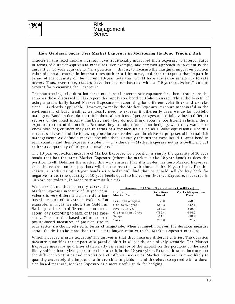
Traders in the fixed income markets have traditionally measured their exposure to interest ratesin terms of duration-equivalent measures. For example, one common approach is to quantify theamount of “10-year equivalents” in a position — that is, to measure the marginal impact on positionvalue of a small change in interest rates such as a 1 bp move, and then to express that impact interms of the quantity of the current 10-year note that would have the same sensitivity to ratemoves. Thus, over time, traders have become comfortable with a “10-year-equivalent” unit ofaccount for measuring their exposure.

The shortcomings of a duration-based measure of interest rate exposure for a bond trader are thesame as those discussed in this report that apply to a bond portfolio manager. Thus, the benefit ofusing a statistically based Market Exposure — accounting for different volatilities and correla-tions — is clearly applicable. However, to make the Market Exposure measure meaningful in theenvironment of bond trading, we clearly need to express it differently than we do for portfoliomanagers. Bond traders do not think about allocations of percentages of portfolio value to differentsectors of the fixed income markets, and they do not think about a coefficient relating theirexposure to that of the market. Because they are often focused on hedging, what they want is toknow how long or short they are in terms of a common unit such as 10-year equivalents. For thisreason, we have found the following procedure convenient and intuitive for purposes of internal riskmanagement: We define a market portfolio that is simply the current most liquid 10-year bond ineach country and then express a trader's — or a desk's — Market Exposure not as a coefficient butrather as a quantity of “10-year equivalents.”

The 10-year-equivalent measure of Market Exposure for a position is simply the quantity of 10-yearbonds that has the same Market Exposure (where the market is the 10-year bond) as does theposition itself. Defining the market this way ensures that if a trader has zero Market Exposure,then the returns on his positions will be uncorrelated with those of the 10-year bond. For thisreason, a trader using 10-year bonds as a hedge will find that he should sell (or buy back fornegative values) the quantity of 10-year bonds equal to his current Market Exposure, measured in10-year equivalents, in order to minimize his risk.

We have found that in many cases, the Amount of 10-Year-Equivalents ($, millions) U.S. Bond Duration- Market-Exposure-Market Sector Based Based

Less than one-year -6.0 -68.3One- to five-year 686.3 732.4Five- to 15-year 389.2 389.4Greater than 15-year -782.4 -944.0Swaps -51.1 -38.3Total 236.0 71.2

Market Exposure measure of 10-year equi-valents is very different from the duration-based measure of 10-year equivalents. Forexample, at right we show the GoldmanSachs positions in different sectors on arecent day according to each of these mea-sures. The duration-based and market-ex-posure-based measures of position size ineach sector are clearly related in terms of magnitude. When summed, however, the duration measureshows the desk to be more than three times longer, relative to the Market Exposure measure.

Which measure is more accurate? The answer is that they measure different entities. The durationmeasure quantifies the impact of a parallel shift in all yields, an unlikely scenario. The MarketExposure measure quantifies statistically an estimate of the impact on the portfolio of the mostlikely shift in bond yields, conditional on a shift in the 10-year yield. Because it takes into accountthe different volatilities and correlations of different securities, Market Exposure is more likely toquantify accurately the impact of a future shift in yields — and therefore, compared with a dura-tion-based measure, Market Exposure is a more useful guide for hedging.

13


III. Market Exposureand the GlobalBond FundManager

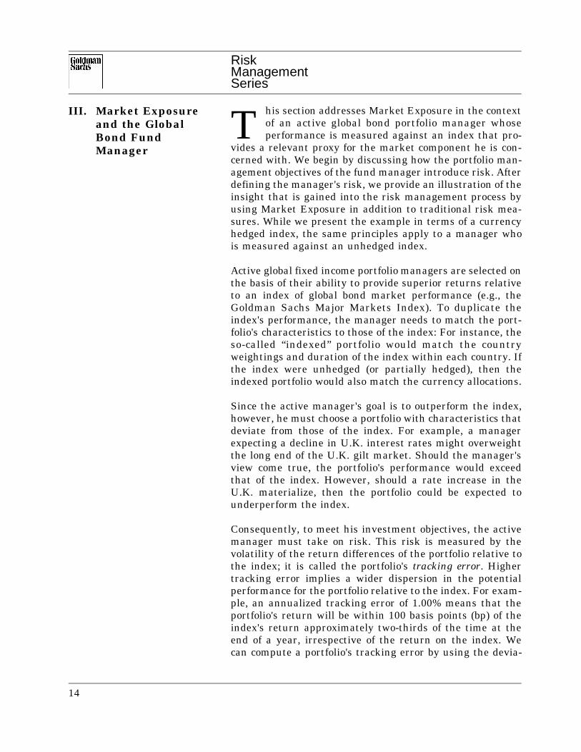
his section addresses Market Exposure in the contextT of an active global bond portfolio manager whoseperformance is measured against an index that pro-

vides a relevant proxy for the market component he is con-cerned with. We begin by discussing how the portfolio man-agement objectives of the fund manager introduce risk. Afterdefining the manager's risk, we provide an illustration of theinsight that is gained into the risk management process byusing Market Exposure in addition to traditional risk mea-sures. While we present the example in terms of a currencyhedged index, the same principles apply to a manager whois measured against an unhedged index.

Active global fixed income portfolio managers are selected onthe basis of their ability to provide superior returns relativeto an index of global bond market performance (e.g., theGoldman Sachs Major Markets Index). To duplicate theindex's performance, the manager needs to match the port-folio's characteristics to those of the index: For instance, theso-called “indexed” portfolio would match the countryweightings and duration of the index within each country. Ifthe index were unhedged (or partially hedged), then theindexed portfolio would also match the currency allocations.

Since the active manager's goal is to outperform the index,however, he must choose a portfolio with characteristics thatdeviate from those of the index. For example, a managerexpecting a decline in U.K. interest rates might overweightthe long end of the U.K. gilt market. Should the manager'sview come true, the portfolio's performance would exceedthat of the index. However, should a rate increase in theU.K. materialize, then the portfolio could be expected tounderperform the index.

Consequently, to meet his investment objectives, the activemanager must take on risk. This risk is measured by thevolatility of the return differences of the portfolio relative tothe index; it is called the portfolio's tracking error. Highertracking error implies a wider dispersion in the potentialperformance for the portfolio relative to the index. For exam-ple, an annualized tracking error of 1.00% means that theportfolio's return will be within 100 basis points (bp) of theindex's return approximately two-thirds of the time at theend of a year, irrespective of the return on the index. Wecan compute a portfolio's tracking error by using the devia-

14


tions of the portfolio from its benchmark's weights, the vola-tilities of the assets in the portfolio and benchmark, and thecorrelations between asset returns.

To outperform the index, the manager can either changeexposure to those factors that affect the index or changeexposure to factors that are not reflected in the index's per-formance. By changing exposure to either of these factors,the manager changes the tracking error. Thus, we want todistinguish between two sources of tracking error: the MarketExposure, or exposure to factors that influence the index re-turn; and the residual risk, or exposure to factors that do notinfluence the index. We will examine each of these in turn.

Market Exposure andPortfolio Performance

A portfolio's Market Exposure is a coefficient that quantifiesthe expected performance of the portfolio for a given indexperformance.

Equation (1) shows the relationship between expected portfo-lio return, index return, and Market Exposure. Portfolio andindex returns are expressed relative to cash — i.e., as re-turns over (or under) the cash rate. Notice that if the Mar-ket Exposure equals 1.0, then we can anticipate that theportfolio's performance will match the index return, all elseequal. However, if the Market Exposure is greater than 1.0,then we can expect the portfolio to outperform the index inrallies and underperform the index in sell-offs. For example,if global interest rate changes have a greater impact on theportfolio than on the index, then the Market Exposure wouldexceed 1.0. As global interest rates decline, the portfolio willoutperform the index, while in sell-offs the portfolio willunderperform the index.

(1)ExpectedPortfolioReturn

MarketExposure × Index

Return

Suppose that the portfolio's Market Exposure is 1.20 andthat the declines in interest rates lead to an index return of10%. In this case, we expect the portfolio's return to be 12%,meaning that the portfolio will outperform the index by 20%.However, if the index return is -10% the portfolio's expectedreturn is -12%, indicating that the portfolio will underper-form the index by 20%.

15


In a domestic portfolio management context, the active man-

Exhibit 2

Correlations Across Markets

France Germany Japan U.K. U.S.

France 1.00Germany .75 1.00Japan .17 .21 1.00U.K. .62 .64 .05 1.00U.S. .36 .41 -.02 .36 1.00

ager who anticipates a rate decline will implement this viewby selecting a portfolio whose duration exceeds that of theindex. For example, suppose that the portfolio and indexdurations are 5.00 and 4.00, respectively. In this case, a 100bp decline in all interest rates is translated into the portfoliooutperforming the index by 1 percentage point, or a 25%outperformance. Similarly, if all interest rates increase by100 bp, the portfolio will underperform the index by 1 per-centage point, or a 25% underperformance. Because in adomestic market all interest rate changes are highly corre-lated, the Market Exposure is approximately the ratio of theportfolio and index durations. In our example, the MarketExposure is about 1.25. Of course, in practice, not all domes-tic interest rates will move by the same amount; therefore,as a measure of exposure for a domestic fixed income portfo-lio, duration may on occasion be highly misleading. Nonethe-less, duration is widely used for risk management in thiscontext.

However, an attempt to extend duration to risk measure-ment for a global fixed income portfolio requires two condi-tions that are not even approximately true. These are (1)that yield volatilities are similar across markets and (2) thatinterest rates movements are highly correlated across mar-kets. If both the portfolio and the benchmark are unhedged(i.e., include currency risk), then a third condition is re-quired: that currency movements and interest rate move-ments are highly correlated.

16


For example, let's consider the first condition. Exhibit 1

Exhibit 1

GS LMI Yield Volatilities

Country 1–3 Years 10+ Years

France 15.12 14.96Germany 13.50 13.00Japan 30.11 12.83U.K. 15.95 14.74U.S. 17.22 12.36

shows the yield volatilities for two of the sectors of the Gold-man Sachs Liquid Market Index™ (GS LMI) in the French,German, Japanese, U.K., and U.S. government bond mar-kets. The two sectors shown in Exhibit 1 are the one- tothree-year and the greater-than-10-year sectors. (We calcu-lated volatilities using daily data covering the period fromFebruary 1988 to March 1995, with a 10% monthly decay.)As the table illustrates, volatilities vary both within marketsand across markets. For instance, while the one- to three-year volatility roughly equals the greater-than-10-year vola-tility in France and Germany, the short sector volatilityexceeds the longer sector volatility in Japan and the UnitedStates. Similarly, the longer sector volatility in Japan is lessthan those of the other markets.

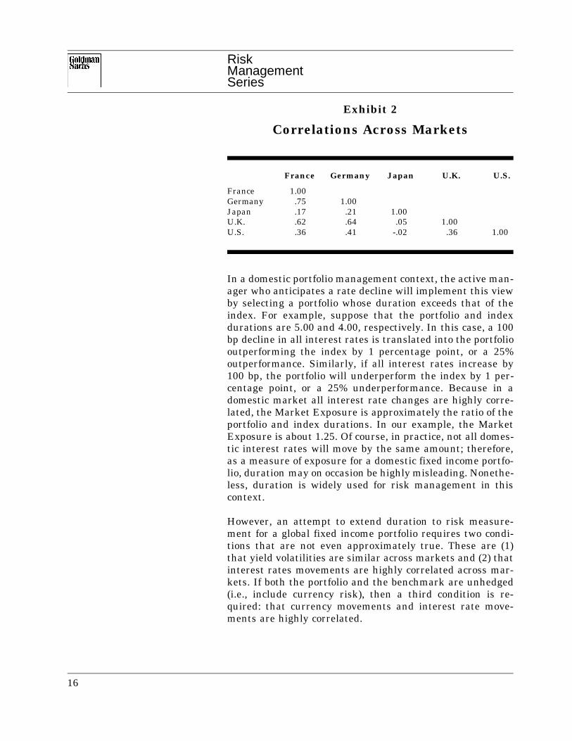
Now let's consider the second condition, that of high corre-lations both across and within markets. As Exhibit 2 makesclear, this condition is also violated in practice. Exhibit 2summarizes the correlations for the GS LMI (full index) forthe five countries shown in Exhibit 1 (we calculated correla-tions using the same data and procedure as in Exhibit 1).Again, inspection of the data in Exhibit 2 indicates that mostof the major markets are not highly correlated. For example,the correlation between the Japanese market and the othermarkets ranges from -0.02 to +0.21. The correlation betweenthe German and French markets is higher than all othercorrelations. By way of comparison, the correlations in theU.S. market range from 0.80 between the one- to three-yearand greater-than-10-year sectors to 0.97 between the seven-to 10-year and greater-than-10-year sectors.

17


The final condition required to justify using duration in the

Exhibit 3

Currency and Bond Correlations

Currency____________________________________________

1–3 Year Sector France Germany Japan U.K.

France -.19 -.23 -.13 -.17Germany -.16 -.15 -.01 -.19Japan .18 .21 .26 .04U.K. -.19 -.21 -.10 -.14U.S. -.05 -.04 -.08 -.03

Exhibit 4

Benchmark Asset Weights

Country Country Weight Country Duration

France 7.70 5.42Germany 12.08 4.36Japan 22.56 5.66U.K. 6.92 5.89U.S. 50.75 5.04

context of an unhedged global fixed income management isthat currency and interest rate movements are highly corre-lated. Exhibit 3 summarizes the correlations between cur-rencies and the GS LMI, using the U.S. dollar as the basecurrency. This table shows the correlation between the re-turn to each currency and the return to the GS LMI(hedged) for all countries. For example, the correlation be-tween the return to the yen and the return to the GS LMIfor the United Kingdom is -0.10; that is, as the yen rallies,the U.K. gilt market sells off. As the table clearly shows,correlations between currencies and bonds have been farfrom highly correlated.

The numbers in Exhibits 1–3 are quite compelling and raisetwo questions: First, does it make any practical difference ifduration is used as a risk measure in a global context? Sec-

18


ond, how is Market Exposure to be computed if duration isnot used?

Looking at the first question, let's suppose that actual yieldvolatilities and correlations are as shown in Exhibits 1–3. Atthe risk of seeming complicated, let's consider a real worldexample. Suppose that a global manager uses the globalduration to calculate the exposure of his portfolio to interestrate changes, and that the manager is measured against anindex whose weights and duration within each country (as ofJanuary 3, 1994) are shown in Exhibit 4. The index — as-sumed to be fully hedged — consists of the market capital-ization weights in the GS LMI for France, Germany, Japan,the United Kingdom, and the United States. Combining theweights and durations of Exhibit 4 leads to a benchmarkduration of 5.2; i.e., for a 100 bp yield decline in all markets,the benchmark's return will be 5.2%.

Now suppose that the manager is bullish on global bondmarkets and expects yields to decline in all five markets.However, he also believes that there will be relative perfor-mance differences between the markets. In particular, sup-pose that the manager believes that the German market willoutperform cash by 208 bp, that the Japanese market willoutperform cash by 159 bp, that the excess return on the U.K.market is 125 bp, that the excess return in the United Statesis 98 bp, and that the worst performing market will be theFrench, which he expects to outperform cash by only 76 bp.

To implement these views, the manager constructs a portfo-lio whose duration is 10% longer than that of the bench-mark; i.e., the portfolio's duration is 5.72 years. Since themanager is concerned about risk control, the portfolio'stracking error is constrained to be 100 bp. The managerbelieves that all yields will decline by 100 bp, the bench-mark will rally by 5.2%, and the portfolio will outperform itby at least 52 bp. Since the manager has views on relativeperformance between markets (or spread views), the portfo-lio could outperform the benchmark by more than 52 bp. Onbalance, then, the manager believes that two sources of riskhave been controlled: First, volatility relative to the indexhas been controlled, since the tracking error has been con-strained at 100 bp. Second, risk from market movementshas been controlled, since the portfolio's duration has beenconstrained to 10% more than the benchmark's duration.

19


How would these constraints have worked in practice? Sup-pose that the manager had developed a portfolio using theseviews and constraints at the beginning of 1994. In this case,the optimal portfolio would have 42.02% of its weight inGerman bonds, 17.42% of its weight in Japanese bonds,1.10% in U.K. bonds, and 39.45% in U.S. bonds. Combiningthese weights with the expected return views means that theportfolio is expected to outperform the benchmark by 81 bp.

Of course, 1994 was a very volatile period for the fixed in-come markets; rather than rally, most markets actually soldoff. Reflecting the market sell-off, the benchmark underper-formed cash by 7.20%. The manager's exposure to marketmoves, as measured by the relative durations, is 1.1(5.67/5.15). Thus, the manager would have anticipated un-derperforming the benchmark by 73 bp, all else equal. How-ever, the portfolio's actual performance in 1994 was -8.52%.In other words, the portfolio underperformed the benchmarkby 132 bp, 60 bp more than would have been predicted bysimply looking at the relative durations.

What went wrong? In developing the optimal portfolio, themanager used the relative durations as the measure of expo-sure to market moves. As discussed above, this approachimplicitly assumes that all markets are perfectly correlated;in other words, all curves move in the same direction at thesame time by the same amount. Exhibits 1–3 clearly demon-strate that this condition is violated in practice.

Now suppose that the manager had decided to recognize thelimitations in using duration, and that he used Market Ex-posure instead of duration. That is, rather than develop aportfolio whose duration was 10% longer than that of thebenchmark, the manager developed a portfolio whose Mar-ket Exposure was 1.1. To achieve this end, he would need toknow the Market Exposures for each of the proposed assetsin the portfolio. Exhibit 5 shows the Market Exposures foreach of the countries in the benchmark, calculated with thevolatilities and correlations of Exhibits 1–3 (i.e., explicitlyrecognizing that interest rate movements are not perfectlycorrelated across and within markets). We can also calculateMarket Exposures for each of the maturity sectors in eachcountry. (Appendix A provides the Market Exposures foreach of the maturity sectors against the capitalization-weighted benchmark.)

20


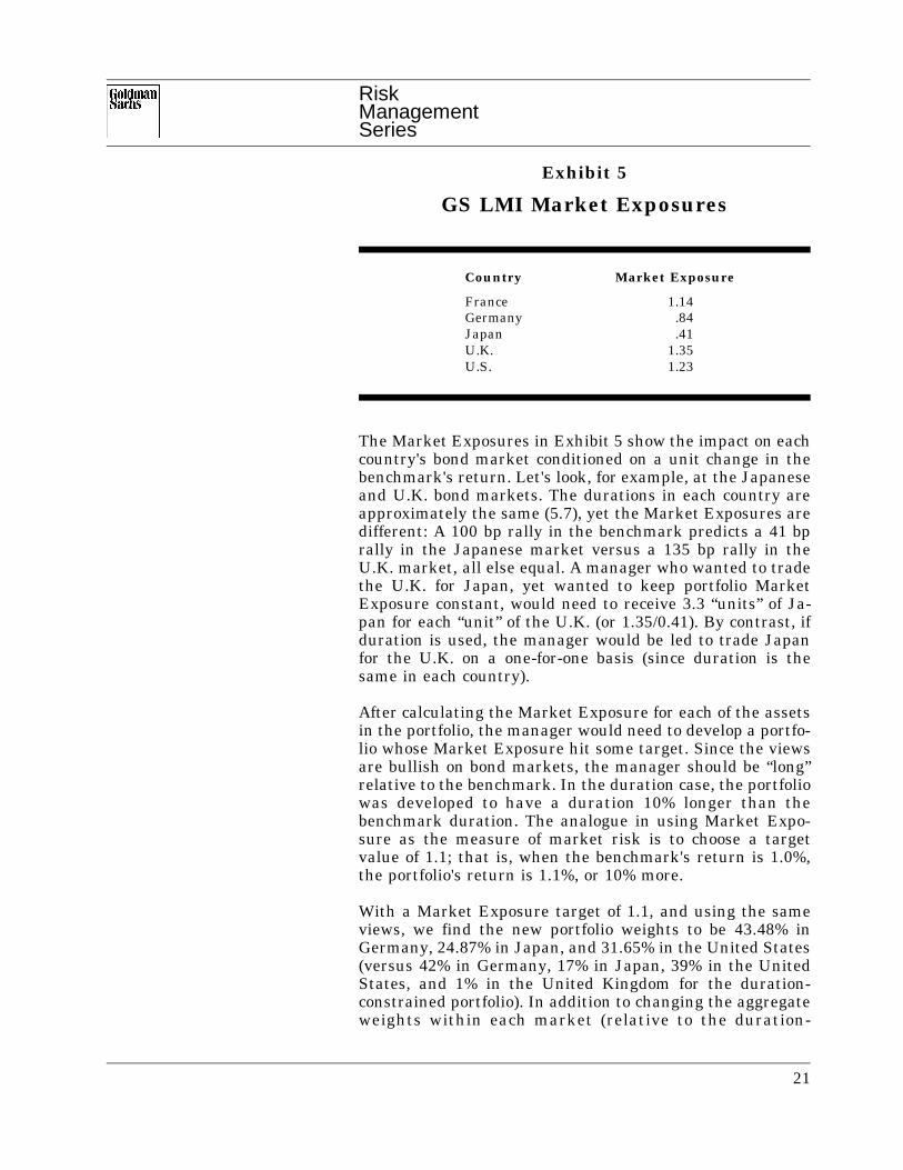
The Market Exposures in Exhibit 5 show the impact on each

Exhibit 5

GS LMI Market Exposures

Country Market Exposure

France 1.14Germany .84Japan .41U.K. 1.35U.S. 1.23

country's bond market conditioned on a unit change in thebenchmark's return. Let's look, for example, at the Japaneseand U.K. bond markets. The durations in each country areapproximately the same (5.7), yet the Market Exposures aredifferent: A 100 bp rally in the benchmark predicts a 41 bprally in the Japanese market versus a 135 bp rally in theU.K. market, all else equal. A manager who wanted to tradethe U.K. for Japan, yet wanted to keep portfolio MarketExposure constant, would need to receive 3.3 “units” of Ja-pan for each “unit” of the U.K. (or 1.35/0.41). By contrast, ifduration is used, the manager would be led to trade Japanfor the U.K. on a one-for-one basis (since duration is thesame in each country).

After calculating the Market Exposure for each of the assetsin the portfolio, the manager would need to develop a portfo-lio whose Market Exposure hit some target. Since the viewsare bullish on bond markets, the manager should be “long”relative to the benchmark. In the duration case, the portfoliowas developed to have a duration 10% longer than thebenchmark duration. The analogue in using Market Expo-sure as the measure of market risk is to choose a targetvalue of 1.1; that is, when the benchmark's return is 1.0%,the portfolio's return is 1.1%, or 10% more.

With a Market Exposure target of 1.1, and using the sameviews, we find the new portfolio weights to be 43.48% inGermany, 24.87% in Japan, and 31.65% in the United States(versus 42% in Germany, 17% in Japan, 39% in the UnitedStates, and 1% in the United Kingdom for the duration-constrained portfolio). In addition to changing the aggregateweights within each market (relative to the duration-

21


constrained portfolio), the distribution across maturities ineach country is different. (Appendix A contrasts the matu-rity distribution for each portfolio.)

The 1994 performance characteristics of the new portfolioare strikingly different from those of the previous portfolio.Using Market Exposure, the portfolio underperforms cash by7.99%, or by 79 bp more than the benchmark. Notice, how-ever, that the portfolio's performance is 113% of the bench-mark's, or roughly what the Market Exposure would predict.Furthermore, the actual tracking error is within the 100 bpband specified by the tracking error constraint.

These results are instructive for determining what wentwrong with the earlier portfolio. Using the Market Expo-sures for each of the assets in the initial portfolio, we calcu-late the overall Market Exposure as 1.18. Consequently, theactual performance of the portfolio relative to the bench-mark is in line with the performance that would be predict-ed by using Market Exposure instead of relative durations.

In this example, the manager was nearly twice as long rela-tive to his benchmark as he wanted to be. As a result, hesuffered nearly twice as much pain! This example illustratesthat correctly measuring Market Exposure can have a majorimpact on portfolio risk management. However, there areother sources of portfolio risk beyond Market Exposure. Wediscuss these briefly below.

Residual Risk andPortfolio Performance

Thus far, our discussion has focused on Market Exposure,i.e., the sensitivity of a portfolio's risk purely to marketmovements. However, portfolio managers can take on riskfrom other sources. For example, suppose that a domesticfixed income manager is measured against a governmentbond index and adopts the following strategy: Maintainduration equal to the index duration but purchase corporatebonds (assuming that this is permissible in the investmentmandate). Since this is a domestic portfolio, the governmentbond Market Exposure is likely to be neutralized by settingthe duration equal to the index duration. However, the port-folio is nonetheless exposed to risk attributable to move-ments in the corporate bond spread.

Alternatively, a global fixed income manager who is mea-sured against a government bond index could pursue thefollowing strategy: Maintain a duration equal to the indexduration in each country but adjust holdings to account for

22


differences in curve shape across countries. For example, hisstrategy might be to position for the convergence of yieldcurve slopes of countries within a currency block. In thiscase, the manager's portfolio again is exposed to risk beyondthe pure movements in the index: The risk this time is afunction of curve shapes.

As a final example, consider again a global fixed incomemanager whose benchmark is a fully hedged index. In thiscase, suppose that the manager's portfolio matches the indexweight, duration, and maturity composition in each country.He seeks to enhance return by taking on currency exposure(even though the benchmark is a fully hedged index). Again,the manager's portfolio is exposed to risks beyond thoseinherent in the index: In this case, the risk is attributable tothe currency exposure.

A consistent feature of all of these examples is that exposureto pure index movements can be neutralized (i.e., MarketExposure equals 1.0), yet the portfolio is still exposed torisk. In this case, the risk is what we have called residualrisk.

Traditional portfolio management focuses only on risk andexpected return. The risk measure in that context does notdistinguish between market risk and residual risk. We be-lieve the distinction is important. Most investors today donot manage their own funds. Individuals and pensions typi-cally make basic asset allocation decisions, such as the pro-portions to invest in equities versus bonds and domesticversus foreign securities, but they hire investment managersto actually invest the funds in the particular asset class. Inthis context, an investment manager who chooses a MarketExposure substantially different from 1.0 relative to hisbenchmark can potentially expose the investor to more mar-ket risk than was intended by the original asset allocationdecision. Since market risks are nondiversifiable, the inves-tor should decide how much of such risk he wants. Residualrisks are diversifiable, and thus the investor should be muchless concerned about the amount of such risks taken by aparticular portfolio manager. Since residual risks are diver-sifiable, there is no risk premium hurdle required to justifytaking such risk. Thus, these are the types of risks thatportfolio managers who are hired to add value through ac-tive management should be encouraged to take.

23


IV. Market Exposureand the GlobalBond Trader

raders and portfolio managers very often try to createTtrade weights that they believe are market-neutral. Inthe fixed income markets, common examples are yield

curve steepening or flattening trades; butterfly positions,long at two points in the curve and short in between, or viceversa; and international spread trades. In the equity mar-ket, examples include being long one stock and short relatedstocks or being long one industry and short another. Incurrencies, a typical example would be a position long onecurrency against a related basket of other currencies. Ineach of these cases, the motivation is the same: to capturethe special relative value of one security versus another, orone sector versus another, without being exposed to thegeneral risk affecting all related securities.

In the absence of a definition of “market-neutral,” or even of“the market,” traders have improvised many schemes forweighting relative value trades. For example, a standardapproach to creating relative value trades in fixed incomemarkets is to weight the legs in such a way that the totalposition has zero duration. This weighting is motivated bythe observation that with such a position, a small parallelshift in yields has no impact on its value. Of course, theproblem with such an approach is that market moves aremost often not associated with parallel shifts — typicallyyield curves steepen in rallies and flatten in sell-offs — andtraders with zero duration weights find that their positionshave a market-directional bias.

In this section, we describe a general approach to creatingmarket-neutral trade weights. We will then compare thisapproach with some alternatives that are commonly used.However, we will not argue that the “market-neutral”weights are necessarily better than alternative weights.What we do maintain is that for any set of weights thereexists a set of implied views — i.e., expected excess returnsfor each security in the trade — for which those weights areoptimal. What is special about the views that motivate a“market-neutral” trade is that they are intended to expressa view about relative value of individual securities or sectorsof the market; they are not intended to express a view on themarket as a whole. Thus, for a market portfolio, the expect-ed excess returns implied by the relative value trade shouldbe zero. After reviewing the relationship between weightingsof trades and views, we will conclude that the market-neu-tral weighting, as defined here, is appropriate whenever thedesire is to express an opinion about relative value.

24


Creating `Market-Neutral'Weights for RelativeValue Trades

We define a market-neutral trade as a set of positions forwhich the aggregate returns are uncorrelated with the re-turns of the market — i.e., with zero Market Exposure.Thus, the first step in a procedure to create market-neutraltrade weights is to identify the market to which the trade isdesigned to be neutral. This is actually the most difficultissue. For example, if the desire is to create a trade that willprofit when German bonds outperform French bonds, then itis not clear to which market the trade should be neutral. Isit the German market, the French market, some combina-tion of the two, or a larger market such as all of Europe?There is no right or wrong answer to this question. We havefound, however, that in practice a simple definition of themarket works best. For example, in this context we mightdefine the market as an equally weighted combination ofFrench and German 10-year bonds. In most contexts, thesimplicity of such a definition far outweighs the potentialbenefits of a more precise measurement.

Given a defined market portfolio, we can state the conditionfor market neutrality of a spread trade quite simply, interms of covariances. By a spread trade, we mean a portfolioof two assets — e.g., the German bond and the French bondin the above example. We will call these two assets “x” and“y.” We label the market portfolio “z.” Let σxz be the covari-ance of asset x and the market portfolio, and let σyz be thecovariance of asset y with the market portfolio. Normalizingon the amount of asset x, we solve for a weight, w, of assety such that the portfolio [x - (w × y)] has zero covariancewith the market portfolio, z. In other words, we solve for aweight, “w,” such that if we short w units of y for each unitof x we obtain a market-neutral portfolio. It is apparent thatthe correct value for w is the ratio of σxz to σyz.

4 How wouldthis work in practice?

We start with the problem of constructing a market-neutralportfolio long German 10-year bonds and short French 10-year bonds. We suppose that the portfolio to which we wantto remain market-neutral is an equally weighted sum ofGerman and French 10-year bonds. Using daily data fromFebruary 1, 1988, through October 6, 1995, and down-weighting older data at a rate of 10% per month, we esti-mate the annualized covariance of the German bond withthis portfolio to be 35.63. The covariance with the French 4 Let p = [x - (w × y)]. The covariance between p and the market, z, is

given as σpz = σxz - wσyz. We want σpz = 0, so we want σxz - wσyz = 0.Solving for w gives us w = σxz /σyz .

25


bond is 42.99. Thus, using the above formula, we shouldshort 35.63/42.99 = 0.8288 units of market value of Frenchbonds for every unit of market value of German bonds. Forexample, a position long $100 million of German bondsshould be hedged with a short position of $82.88 million ofFrench bonds.

More generally, when the market-neutral portfolio that weare trying to construct has more than two assets, then thereis no unique set of weights. In general, market neutralityimposes a condition, a linear constraint, that the relativeweights of other assets in the portfolio must satisfy. Again,we normalize the weights relative to one unit of security x.Consider a portfolio of assets x and y(1), y(2) . . . y(n) de-fined by [x - Σ aj × y(j)]. Again we let z represent the marketportfolio. Let σy(j)z represent the covariance of asset y(j) withthe market and σxz represent the covariance of asset x withthe market. In this case, the condition for market neutralityis that Σajσy(j)z = σxz. Notice that the situation of two-assetweights is a special case where aj equals zero for all but oneasset.

In many cases, traders may have access to volatilities ofindividual assets but not to the covariances of those assetswith each other or a market portfolio. In the context of aspread trade, we can simplify matters further and avoid thisproblem if we adopt as the market portfolio a positivelyweighted average of the two assets where the weights areinversely proportional to their volatilities — that is, if wedefine the market portfolio to be a linear combination of theassets in which each asset contributes equally to volatility.In this special case, which is actually a rather intuitivedefinition of the market portfolio, the market-neutral portfo-lio is also a portfolio in which each asset contributes equallyto volatility — except that while the market portfolio is longboth assets, the market-neutral portfolio is long one assetand short the other. For example, in the case of German andFrench bonds, the volatilities of the bonds are 6.03 and 7.14,respectively. The ratio of German volatility to French vola-tility is 0.8436. Thus, using a market portfolio with 1.0 unitof German bond market value per 0.8436 unit of Frenchbond market value, the market-neutral portfolio must short0.8436 unit of French bonds for each unit of German bonds.For a position long $100 million of German bonds, we re-quire a short of $84.36 million of French bonds. Notice thatthe size of the hedge position is relatively insensitive to thecomposition of the market portfolio.

26


As another example, let us consider a butterfly trade in U.S.bonds long the five-year benchmark and short the two-yearand 10-year benchmarks. This position will look attractivewhen the yield curve is unusually curved — i.e., the five-year yield is high relative to a weighted average of the two-and 10-year yields, and the yield curve is expected tostraighten. To simplify matters, we consider a market port-folio defined as equal weights of each bond. The covariancesof the two-year, the five-year, and the 10-year bond with thismarket portfolio are 10.55, 24.84, and 37.48, respectively.Thus, using the formula given above, for each unit of thefive-year bond long, we must short a weighted average oftwo- and 10-year bonds using weights w2 and w10 such thatw2×10.55 + w10×37.48 = 24.84. There are many such pairsof relative weights that we could use. For example, we couldpick weights to match the value in both sides of the trade —i.e., we could also require that w2+w10 = 1. Using this addi-tional constraint, we would require short positions of 46.94in two-year bonds and 53.06 in 10-year bonds against a longposition of $100 million in the five-year bond. Although thisweighting is market-neutral, as we shall see, it may notexpress the relative value view that is desired.

Let us revisit this butterfly trade and consider another pos-sible constraint. Remember that the motivation for the tradewas to benefit from a straightening of the yield curve. Thus,in addition to being market-neutral, we might also want toinsulate ourselves from a flattening or a steepening of theyield curve. A natural way to do this is to weight the tradeso that it is also neutral relative to a portfolio constructed tohave returns sensitive to such moves.

To accomplish this, we follow a procedure analogous to thatused in creating a market-neutral set of weights. First, weconstruct a market-neutral portfolio long two-year bonds andshort 10-year bonds. This portfolio, which we call the “steep-ening” portfolio, has 10.55/37.48 = 0.2814 unit of 10-year perunit of two-year (based on the above reported covariances).We then measure the covariances between the individualbonds and the steepening portfolio returns. We find that thetwo-, five-, and 10-year bonds have covariances of 57.38,18.70, and -105.51, respectively, with the steepening portfo-lio. Thus, the “market” and “steepening” neutral portfoliomust have weights w2 and w10 such that, as above,

w2×10.55 + w10×37.48 = 24.84, and also thatw2×57.38 + w10×(-105.51) = 18.70.

27


Simple algebra reveals that the appropriate short positionsare $101.77 million in two-year bonds and $37.63 million in10-year bonds against the long position of $100 million inthe five-year bond. Notice that neutralizing with respect tosteepening or flattening of the yield curve has a substantialeffect on the weights.

Alternative Approaches How do these market-neutral weights compare with morefamiliar trade weightings? We return to the German bondversus French bond example. The most common weightingwould be to match the durations of each side of the trade.Given durations of 6.72 and 6.61, respectively, for the Ger-man and French bonds, the “duration-neutral” weight inFrench bonds is $101.66 million against a $100 million longposition in German bonds. The problem with such weights,as many traders could testify, is that the French market isgenerally more volatile than the German market. Thus, sucha trade will perform well in sell-offs and suffer in risingmarkets. That is, such weights are not market-neutral.

Another common approach to hedging is to use “regression”weights. This approach is motivated by the desire to find the“best hedge” using French bonds against the long position inGerman bonds. The best hedge — that is, the position thatminimizes volatility — is given by the coefficient in theregression of German bond returns on French bond returns.That regression coefficient is the ratio of the covariance ofGerman and French bonds to the variance of the Frenchbonds. That covariance, using the same data as mentionedabove, has a value of 34.91, and the variance of Frenchbonds is 51.07. Thus, the regression coefficient is 0.6835,and the best hedge of the German $100 million position is ashort French position of $68.35 million. Notice, first, thatsuch an approach is not symmetric between the markets.The best hedge of a short position in French bonds usingGerman bonds does not lead to the same relative weights inthe markets as does the best hedge of a long position inGerman bonds using French bonds. In other words, thereader may verify (using the fact that German bond vari-ance is 36.35) that the best hedge of a short French bondposition of $68.35 is not a long German position of $100million but rather a long German bond position of only$65.63 million. Although it may not be obvious, it turns outthat relative to any market portfolio consisting of positiveweights in the two bonds, the best hedge of the long Germanposition using French bonds will always create a portfoliowith a long market-directional bias. And the best hedge of

28


the short French position using German bonds will alwayscreate a portfolio with a short market-directional bias. (Wederive this result in Appendix B.)

A third common approach to hedging a spread trade is tomatch volatility-weighted durations. This approach is moti-vated by the well-known problem of market directionalityobserved above with respect to trades that match durationsdirectly. The volatility-weighted duration trade scales theduration of one side of the trade by the relative volatilitiesof the yield changes in the two markets. To illustrate, in theabove example we find that French 10-year bond yields are20.6% more volatile than German bond yields (measured inbasis points, the German annualized volatility is 89.7 andthe French is 108.2). Thus, to remove the market-directionalbias, it seems natural to use 20.6% less duration in Frenchbonds than in German bonds. For a position long $100 mil-lion of German bonds, we short $84.34 million of Frenchbonds rather than $101.66 million. Perhaps surprisingly,this approach actually works quite well. Notice first that inthis example, the weight in French bonds is almost exactlywhat we discovered above in the example where we used thereturn volatility ratio — which was motivated by the sim-plicity that obtains from defining the market portfolio tohave equal volatility contributions from each bond. This isnot an accident. Yield volatility (measured in basis points)times duration is a reasonably good approximation of returnvolatility. Thus, the volatility-weighted duration approachwill generally be a quite good approximation of a market-neutral weighting — at least relative to this particular mar-ket weighting!

We have now gone through several examples of market-neutral weightings of trades and compared them with alter-native weightings. However, as we stated at the top of thissection, we do not wish to argue that market-neutralweights are always better than alternative weights. Rather,we show in Appendix B that there is a mapping betweenviews — defined as expectations of future excess returns onassets — and optimal weights. Thus, just as we can find anoptimal portfolio for any set of expected returns, we canback out a set of implied views for which any given portfolioweighting is optimal. In this sense, we cannot argue that amarket-neutral portfolio is better than some alternativeweighting without considering the implications of the alter-native weights for expected returns.

29


What we can show in Appendix B is an intuitive result: thata portfolio is market-neutral if, and only if, it implies a zeroexpected excess return on the market portfolio. A portfoliowith a positive Market Exposure will imply a positive ex-pected excess return on the market, while a portfolio with anegative Market Exposure will imply a negative expectedexcess return on the market. Thus, we can make precise thesense in which a market-neutral portfolio may be desirable.Market neutrality is a desirable condition if, and only if, wedo not wish to express a view about the expected excessreturns of the market. We would characterize this conditionof market neutrality as a minimum condition for a “relativevalue” trade, and we thus conclude that the use of market-neutral weights, as defined here, is an appropriate consider-ation for all relative value trades.

30


V. Summary andConclusions

his paper has addressed the measurement and man-Tagement of market risk from the perspective of theglobal bond fund manager and the global bond trader.

We began by describing the fund manager's (or trader's)problem as seeking to outperform some benchmark portfoliowhile simultaneously controlling risk. We then discussedhow, under ideal circumstances, the manager would deter-mine a set of “risk factors” that would be responsible for thereturns of the manager's portfolio. We proceeded to arguethat while this ideal is not easily achieved, managers (ortraders) can nonetheless identify what is generally the mostimportant risk factor, their portfolio's Market Exposure.

After discussing the advantages of making broader use ofcorrelations across markets in describing market risk, weproceeded to demonstrate, through specific examples, howthe use of our measure of Market Exposure could improveportfolio performance and risk control. We showed that fora global bond fund manager, our Market Exposure measureprotected a portfolio's performance, even given views thatwere the exact opposite of actual market moves. We con-trasted market risk with residual risk, arguing that activemanagers can add value by exploiting opportunities that addresidual risk while controlling market risk. One advantageof this approach is that residual risk can be easily diversi-fied, while market risk cannot.

For traders, we examined the problem of identifying weightsfor relative value trades that are intended to be market-neutral. We first offered a definition of market neutralityand then showed how our measure of Market Exposureprovides a set of trade weights that are neutral with respectto market moves. We contrasted the trade weights providedby our measure of Market Exposure with alternative meth-ods and discussed how (and why) they differed.

Our conclusion is straightforward: By explicitly accountingfor the volatilities and correlations of different assets, ourmeasure of Market Exposure can result in improved port-folio management.

31


Appendix AOptimal Portfolio Constraints and Weights

This appendix shows the maturity sector weights for the benchmark and the two optimalportfolios described in Section III. We also describe the constraints used in developing the twoportfolios.

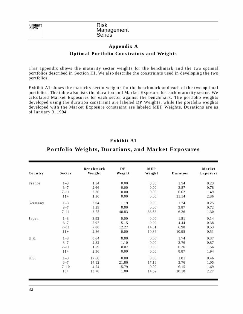
Exhibit A1 shows the maturity sector weights for the benchmark and each of the two optimalportfolios. The table also lists the duration and Market Exposure for each maturity sector. Wecalculated Market Exposures for each sector against the benchmark. The portfolio weightsdeveloped using the duration constraint are labeled DP Weights, while the portfolio weightsdeveloped with the Market Exposure constraint are labeled MEP Weights. Durations are asof January 3, 1994.

Exhibit A1

Portfolio Weights, Durations, and Market Exposures

Benchmark DP MEP MarketCountry Sector Weight Weight Weight Duration Exposure

France 1–3 1.54 0.00 0.00 1.54 0.233–7 2.66 0.00 0.00 3.87 0.787–11 2.20 0.00 0.00 6.62 1.4911+ 1.30 0.00 0.00 11.14 2.36

Germany 1–3 3.04 1.19 9.95 1.74 0.253–7 5.29 0.00 0.00 3.87 0.727–11 3.75 40.83 33.53 6.26 1.30

Japan 1–3 3.92 0.00 0.00 1.81 0.143–7 7.97 5.15 0.00 4.44 0.387–11 7.80 12.27 14.51 6.90 0.5311+ 2.86 0.00 10.36 10.95 0.51

U.K. 1–3 0.64 0.00 0.00 1.74 0.373–7 2.32 1.10 0.00 3.76 0.877–11 1.59 0.07 0.00 6.26 1.5611+ 2.36 0.00 0.00 8.87 1.94

U.S. 1–3 17.60 0.00 0.00 1.81 0.463–7 14.82 21.86 17.13 3.76 1.057–10 4.54 15.79 0.00 6.15 1.6910+ 13.78 1.80 14.52 10.18 2.27

32


We obtained the overall portfolio duration and Market Exposure for each portfolio by takingappropriate weighted averages of the duration and Market Exposure columns. For example,the duration of the benchmark portfolio is 5.15, while the duration of the duration-constrainedportfolio is 5.67 and that of the Market Exposure-constrained portfolio is 6.53. Similarly, theMarket Exposure of the Market Exposure-constrained portfolio is 1.10, while that of theduration-constrained portfolio is 1.17.

In developing the optimal portfolios shown in Exhibit A1 and discussed in Section III, we usedthe following assumptions: In both portfolios, we constrained the tracking error (standarddeviation of the excess return over the benchmark) to be 100 bp. We also assumed that bothportfolios were currency hedged into U.S. dollars, as was the benchmark. To control exposureto market movements, we constrained the first portfolio's duration to be 10% more than thatof the index and the second portfolio's Market Exposure to be 1.1.

Of course, optimization requires expected excess returns. We used the following process todevelop excess returns across each market: In the first step, we projected yield changes for theseven- to 11-year (or 10-year for the United States) sector in each market. For France andGermany, we assumed that yields in the seven- to 11-year sector declined by 10 and 20 bp,respectively, while we projected that Japanese yields would not change from their January1994 levels. In the United Kingdom and the United States, we projected yields to decline by5 and 13 bp, respectively.

In the second step, we used the projected yield changes in the seven- to 11-year (or U.S. 10-year) sector to determine projected excess returns for the sector. Finally, we combined theexpected excess returns for the seven- to 11-year sector with the correlation matrix of excessreturns (as of January 1994) to develop excess returns for each of the remaining sectors.5 Wecombined these projected excess returns with the market capitalization weights to obtain theprojected returns across each market discussed in Section III.

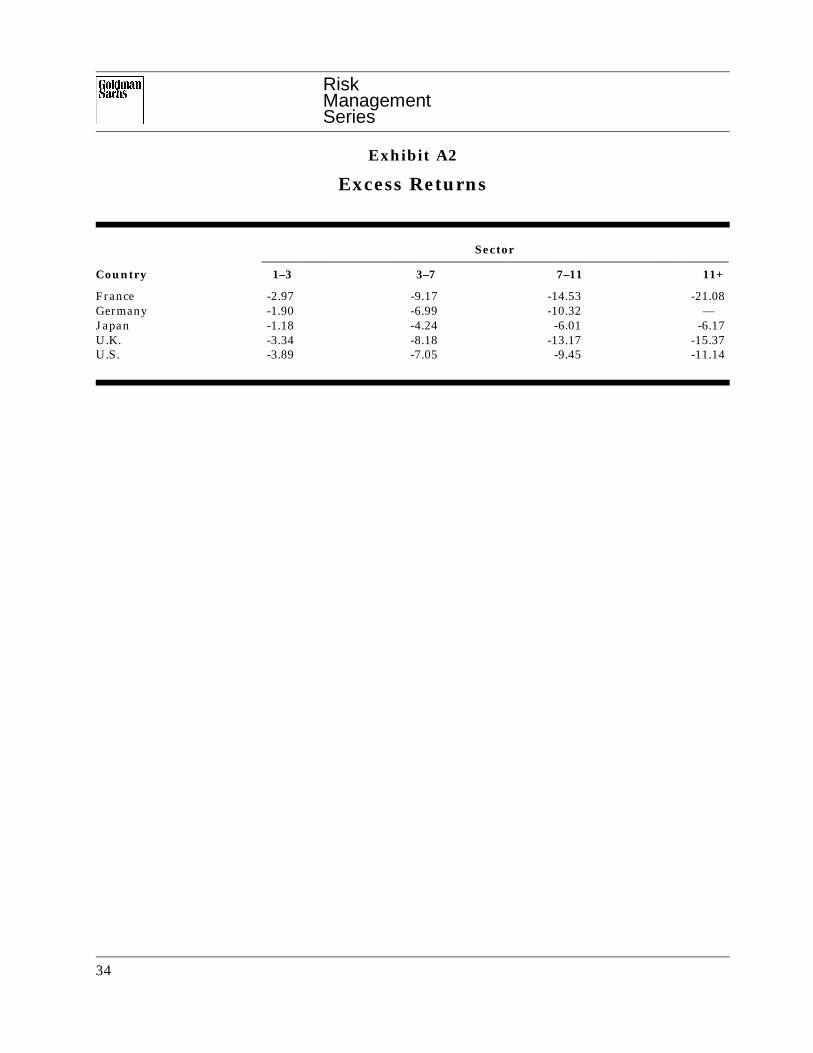
Exhibit A2 shows the actual excess returns for 1994 (i.e., returns over cash) for each of thematurity sectors. We calculated excess returns for each of the portfolios (including the bench-mark) shown in Exhibit A1 by combining the weights in Exhibit A1 with the excess returnsof Exhibit A2. Using this procedure, we found the excess return on the benchmark over 1994to be -7.20, while the excess return on the duration-constrained portfolio was -8.52 and theexcess return on the Market Exposure portfolio was -7.99.

5 The procedure for implementing this calculation is described in Fischer Black and Robert Litterman, Global

Asset Allocation With Equities, Bonds, and Currencies, Goldman, Sachs & Co., October 1991.

33


Exhibit A2

Excess Returns

Sector_____________________________________________________________________________

Country 1–3 3–7 7–11 11+

France -2.97 -9.17 -14.53 -21.08Germany -1.90 -6.99 -10.32 —Japan -1.18 -4.24 -6.01 -6.17U.K. -3.34 -8.18 -13.17 -15.37U.S. -3.89 -7.05 -9.45 -11.14

34


Appendix BThe Mapping Between Views and Portfolio Weights

Even in its simplest form, portfolio optimization is generally considered mathematically as aquadratic optimization subject to linear constraints. However, when we wish to consider themapping between views and portfolio weights, we can solve for a unique mapping only in thecase where constraints are not binding. We generally make this assumption in solving forimplied views, which allows us to simplify the problem considerably.

Let us assume that a portfolio manager has a set of expected excess returns given by thevector µ for a given set of assets. Suppose the covariance matrix of those assets is given by Σ.Then, if we assume that no constraints are binding, the optimal portfolio weights — those thatprovide the greatest expected excess return for a given degree of risk — are proportional to avector w, where w = (Σ)-1 m. Of course, these weights are not unique unless we specify aparticular level of risk. Clearly, we can invert this mapping, at least up to a scale factor. Thatis, given a set of weights, w, and assuming that no constraints are binding, we can solve fora vector µ, where µ = Σw. This vector, and all positive scalar multiples of it, will provide a setof expected excess returns such that the given portfolio weights, w, are optimal relative tothose views.

The first point to make is that a portfolio is market-neutral if, and only if, the implied view ofthe return on the market portfolio is zero. This follows directly from the formula for impliedviews. Let the market portfolio weights be given by a vector, m. A market-neutral portfolio isone for which the covariance of the returns of the portfolio with the returns of the marketportfolio is zero. This covariance is given by the expression [m Σw]. Notice that the expectedreturn on the market portfolio is given by [m µ]. By the above expression for µ, it is clear thatthis expected return on the market portfolio is also given by the expression [m Σw]. Thus, theresult follows.

Why Regression Hedges Are Never Market-Neutral

The next point concerns the implied view of a risk-minimizing spread portfolio, relative to amarket portfolio that includes positive weights in each of the two assets. As above, for a givenportfolio, w, the implied expected excess return on the market is given by [m Σw]. Here weassume that the market weight vector, m, consists of two positive weights, m1 and m2, andthat the portfolio weights in the trade are given by w1 and w2, where either w1 = 1 and w2 =-β (in which case we wish to show that the implied view on the market is positive), or w1 = -1and w2 = β (in which case we wish to show that the implied view on the market is negative).The regression coefficient, β, is given by the ratio σxy to σyy where again we adopt the notationx and y to represent the first and second assets, respectively. First consider the case in whichthe weights are w1 = 1 and w2 = -β. The form [m Σw] can be written as a sum, m1×σxw +m2×σyw. Here we use σxw and σyw to represent the covariances of the returns of asset x andasset y, respectively, with the trade returns using the weights, w. To demonstrate that thissum is positive, we show first that σyw is, by construction, zero. We then show that σxw isnonnegative and can be zero only if the two assets have a correlation of 1.0, which, becausethey are distinct, we assume is not the case. That σyw is zero will not surprise those familiar

35


with regression theory. This is the covariance of a variable with the residuals of a regressionon that variable.

In particular, given the weights in the spread trade, the expression for this covariance is givenby σyw = (σxy - β×σyy). Substitution for β leads to the result. Similarly, if we write out theexpression for σxw, we obtain σxw = (σxx - β×σxy) = σxx × (1 - ρ2), where ρ is the correlationcoefficient between x and y. Thus, we see that the implied expected excess return on themarket portfolio must be positive. The case where the signs are reversed follows similarly,with the conclusion that regression hedging will always create a positive implied view on themarket when the variable being hedged is long and a negative view on the market when thevariable being hedged is short.

36

risk management series -...

Documents