risk management in smes using data mining methods with
TRANSCRIPT

Risk Management in SMEs using Data Mining Methods with
Financial and Non-financial Indicators
A thesis submitted for the degree of Doctor of Philosophy
By
Chenyang He
Brunel Business School
Brunel University London, UK
August 2018

2
Abstract
As the economy develops, the importance of risk management increases significantly.
Newly-developed data mining techniques have also provided an extended range of
information for decision-makers and scholars about the Risk Management (RM)
process. This study thus assessed the use of financial and non-financial indicators in
the RM process based on a Business Intelligence (BI) approach and using data mining
(DM) methodology. Its assessment focused on the selection of Key Risk Indicators
(KRIs) among the various risk indicators for performance measurement and risk
control. This study used a sample of 853 Chinese SMEs listed on the Shenzhen Stock
Exchange. After comparison of LR, GA, NN, and CHAID, CHAID was found to be
the most suitable mode, as it incorporates both financial and non-financial indicators
and is also able to provide roadmaps to improve RM performance. This study also
used a BI approach to quantify and standardise information from government reports
and firms’ annual reports to better generalise the available information for non-
financial indicators. Four different types of risks were considered, following the
enterprise risk management (ERM) framework, and using CHAID as the underlying
method, the threshold values and roadmaps of the KRIs were thus identified. This
study thus provides an integrated method for the risk management process in SMEs
by using both financial and non-financial information generalised using a BI approach
with the DM process. The critical contribution of this study is its combination of the
DM process and RM process, which also allowed examination of the usefulness of
non-financial indicators in the RM process with the ERM framework. Additionally, it
provides practical guidance for using a BI approach for capturing information and
transferring data.

3
Acknowledgement
I would like to express my deep gratitude to my supervisor Dr. Kevin Lu. I am thankful
for his guidance, valuable comments and constructive suggestions throughout my PhD
journey. I am honoured and proud to be one of Dr. Lu’ students and work under his
supervision.
I would like to extent my sincere gratitude to my wife Yu Ge, and my parents, who
have provided me through moral and emotional support in my life.
Last but not least, I am grateful to all my friends and PhD colleagues with whom I
shared my PhD journey.

4
Publications Associated with this Thesis
Journal paper
He C., and Lu K., 2018. The Value of Non-Financial Indicators in Risk Management
and Data Mining: Evidence from listed Chinese SMEs, European Journal of
Operational Research (Under review)
Conference paper
He C., and Lu K., 2018. Risk management in SMEs with financial and non-financial
indicators using Business Intelligence methods, Management, Knowledge and
Learning International Conference 2018.

5
CONTENT
ABSTRACT .......................................................................................................................................... 2
PUBLICATIONS ASSOCIATED WITH THIS THESIS ................................................................. 4
ABBREVIATIONS............................................................................................................................... 9
LIST OF FIGURES ............................................................................................................................ 10
LIST OF TABLES .............................................................................................................................. 13
1. INTRODUCTION ...................................................................................................................... 1
1.1 BACKGROUND .............................................................................................................................. 1
1.2 EXISTING STUDIES IN RISK MANAGEMENT FOR SMES ............................................................... 11
1.3 RESEARCH AIMS ......................................................................................................................... 19
1.4 RESEARCH OBJECTIVES .............................................................................................................. 20
1.5 RESEARCH QUESTIONS ............................................................................................................... 21
1.6 RESEARCH CONTRIBUTIONS ....................................................................................................... 22
1.7 THESIS STRUCTURE .................................................................................................................... 24
1.8 SUMMARY .................................................................................................................................. 25
2. LITERATURE REVIEW .............................................................................................................. 27
2.1 THE DEVELOPMENT OF RISK MANAGEMENT .......................................................................... 27
2.2 THE ISO 31000 FRAMEWORK ................................................................................................. 30
2.3 THE COSO ENTERPRISE RISK MANAGEMENT FRAMEWORK .................................................. 35
2.4 THE CONCEPTS OF RISK MANAGEMENT ................................................................................. 42
2.4.1 Introduction ....................................................................................................................... 42
2.4.2 Enterprise Risk Management Risk types ............................................................................ 44
2.4.3 Risk Management in SMEs ........................................................................................... 54
2.4.4 Indicators in Risk Management .................................................................................... 67
2.4.5 Data Mining and Business Intelligence ........................................................................ 74
2.5 GAP ANALYSIS ........................................................................................................................ 77

6
2.6 SUMMARY ............................................................................................................................... 83
3. DEVELOPMENT OF THE THEORETICAL FRAMEWORK FOR RISK MANAGEMENT
IN SMES ............................................................................................................................................. 85
3.1 INTRODUCTION ........................................................................................................................... 85
3.2 THEORETICAL BACKGROUND ..................................................................................................... 85
3.2.1 The ERM Framework ........................................................................................................ 86
3.2.2 The Risk Management Process .......................................................................................... 93
3.2.3 The Early Warning System ................................................................................................. 96
3.2.4 The Data Mining Process ................................................................................................ 100
3.3 THE CONCEPTUAL MODEL ....................................................................................................... 103
3.4 HYPOTHESES DEVELOPMENT ................................................................................................ 113
3.4.1 Data Mining Process and Risk Management process ...................................................... 114
3.4.2 ERM Framework, KPIs and KRIs .................................................................................... 116
3.4.3 Early Warning System and Risk Treatment ...................................................................... 119
3.4.4 BI approach and SMEs .................................................................................................... 121
3.5 SUMMARY ............................................................................................................................. 122
4. RESEARCH METHODOLOGY ................................................................................................ 125
4.1 INTRODUCTION ......................................................................................................................... 125
4.2 RESEARCH DESIGN ................................................................................................................... 125
4.3 DATA COLLECTION ................................................................................................................... 128
4.4 VARIABLE SELECTION .............................................................................................................. 136
4.5 METHODS INTRODUCTION ........................................................................................................ 141
4.5.1 Decision tree .................................................................................................................... 141
4.5.2 Logit Regression .............................................................................................................. 146
4.5.3 Genetic algorithms........................................................................................................... 149
4.5.4 Artificial Neural Network ................................................................................................ 152
4.5 SUMMARY ................................................................................................................................ 155

7
5 RESULTS AND ANALYSIS .................................................................................................. 157
5.1 INTRODUCTION ......................................................................................................................... 157
5.2 INDICATORS SELECTION ........................................................................................................... 157
5.2.1 Financial and Non-financial Indicators .......................................................................... 157
5.2.2 K-means Clustering ......................................................................................................... 164
5.3 CHAID RESULTS ...................................................................................................................... 167
5.3.1 CHAID algorithms ........................................................................................................... 167
5.3.2 Dependent variable: Z-score ........................................................................................... 168
5.3.3 Dependent variable: growth of ROA; .............................................................................. 181
5.3.4 Summary .......................................................................................................................... 192
5.4 LOGIT REGRESSION RESULTS ................................................................................................... 210
5.4.1 Logit Regression .............................................................................................................. 210
5.4.2 Logit Regression with financial and non-financial indicators ......................................... 211
5.4.3 Logit Regression with financial indicators ...................................................................... 214
5.4.4 Logit Regression with non-financial indicators ............................................................... 216
5.4.5 Summary .......................................................................................................................... 218
5.5 GENETIC ALGORITHM RESULTS ................................................................................................ 221
5.5.1 Genetic Algorithm in variable selection .......................................................................... 221
5.5.2 Genetic Algorithm with financial and non-financial indicators ...................................... 222
5.5.3 Genetic Algorithm with financial indicators .................................................................... 224
5.5.4 Genetic Algorithm with non-financial indicators ............................................................ 226
5.5.5 Summary .......................................................................................................................... 228
5.6 NEURAL NETWORK RESULTS .................................................................................................... 231
5.6.1 BPNN ............................................................................................................................... 231
5.6.2 BPNN with financial and non-financial indicators .......................................................... 233
5.6.3 BPNN with financial indicators ....................................................................................... 236
5.6.4 BPNN with non-financial indicators ................................................................................ 238
5.6.5 Summary .......................................................................................................................... 240

8
5.7 SUMMARY ................................................................................................................................ 244
6. DISCUSSION .......................................................................................................................... 246
6.1 INTRODUCTION ..................................................................................................................... 246
6.2 SELECTION OF KPI ............................................................................................................... 247
6.3 SELECTION OF KRIS ............................................................................................................. 248
6.4 RESULT EVALUATION ............................................................................................................ 254
6.5 HYPOTHESES VERIFICATION ................................................................................................. 259
6.6 COMPARISON WITH OTHER STUDIES ...................................................................................... 266
6.7 SUMMARY ............................................................................................................................. 267
7. CONCLUSION ....................................................................................................................... 269
7.1 OVERVIEW ................................................................................................................................ 269
7.2 ACHIEVEMENTS OF AIMS, OBJECTIVES AND RESEARCH QUESTIONS........................................... 270
7.3 CONTRIBUTIONS ....................................................................................................................... 276
7.3.1 Theoretical Contributions ................................................................................................ 276
7.3.2 Practical Contributions ................................................................................................... 277
7.4 LIMITATION .............................................................................................................................. 279
7.5 RECOMMENDATION .................................................................................................................. 280
7.6 SUMMARY ................................................................................................................................ 282
8. REFERENCE.......................................................................................................................... 284
APPENDICES ...................................................................................................................................... 1
APPENDIX 1: RESULTS OF CHAID ...................................................................................................... 1
APPENDIX 2: RESULTS OF BPNN ........................................................................................................ 7

9
Abbreviations
AUC Area Under Curve
BI Business Intelligence
BPNN Back Propagation Neural Network
CART Classification and Regression Trees
CAS Casualty Actuarial Society
CHAID Chi-square Automatic Interaction Detector
COSO Committee of Sponsoring Organisations of the Treadway Commission
DLI Development and Life Index
DM Data Mining
EWS Early Warning System
ERM Enterprise Risk Management
F and NF Financial and Non-Financial
GAs Genetic Algorithms
ISO International Organization for Standardization
KDD Knowledge Discovery in Databases
KRI Key Risk Indicator
KPI Key Performance Indicator
LR Logit Regression
MDA Multiple Discriminant Analysis
NSBC National Statistical Bureau of China
NN Neural Network
ST Special Treatment
SMEs Small and Medium sized Enterprises
RM Risk Management
RMSE Root Mean Square Error
ROC Receiver Operation Characteristic

10
List of Figures
Name Page
Figure 2.2 The ISO standard risk management process 32
Figure 2.3 The COSO 2013 framework cube 38
Figure 2.4.2 ERM risk catalogues 43
Figure 2.4.5-a Collectable information types by BI 73
Figure 2.4.5-b The Process of BI 73
Figure 2.4.5-c Elements in Data Mining 74
Figure 3.2.1-a The Risk management cycle with ERM 86
Figure 3.2.1-b The Use of KRIs 88
Figure 3.2.2 The ISO standard risk management process 89
Figure 3.2.3 The Process of establishing EWS 94
Figure 3.2.4 Data mining Steps 97
Figure 3.3-a The Detailed RM process 100
Figure 3.3-b Flowcharts of DM-RM model 102
Figure 3.3-c The Research Conceptual model of DM-RM model 103
Figure 3.4 Flowcharts of DM-RM model 110
Figure 3.5 Research Questions 118
Figure 4.2 The Detailed DM process 120
Figure 4.3 List of F and NF indicators 129
Figure 4.4 ERM risk catalogues 131
Figure 4.5.1.1 The Process of CHAID 139
Figure 4.5.2 The Process of LR 142
Figure 4.5.3 The Process of GAs 146
Figure 4.5.4-a The Structure of BPNN 147
Figure 4.5.4-b The Process of BPNN in flowcharts 148

11
Figure 5.2.1 The Frequency of locations 159
Figure 5.2.2 The Result of K-means 162
Figure 5.3.4-a The Visualisation of Feature importance 203
Figure 5.3.4-b The Result of ROC curve of CHAID (ROA) 206
Figure 5.4.2-a The Result of LR with F and NF indicators 208
Figure 5.4.3-a The Result of LR with F indicators 211
Figure 5.4.4-a The Result of LR with NF indicators 213
Figure 5.4.5-a Significant indicators in all LR models and feature importance 217
Figure 5.5.2-a The Result of GA with F and NF (2) 220
Figure 5.5.2-b The Features Importance of GA with F and NF Indicators 221
Figure 5.5.3-a The Result of GA with F indicators (2) 222
Figure 5.5.3-b The Features Importance of GA with F Indicators 223
Figure 5.5.4-a The Result of GA with NF indicators (2) 224
Figure 5.5.4-b The Features Importance of GA with NF Indicators 225
Figure 5.5.5-a The Prediction accuracy of all GA models 226
Figure 5.5.5-b Significant indicators of GA models 228
Figure 5.6.2-a The Result of BPNN with F and NF indicators 230
Figure 5.6.2-b The Prediction accuracy of BPNN with F and NF indicators 231
Figure 5.6.2-c ROC curve of BPNN with F and NF indicators 231
Figure 5.6.3-a The Result of BPNN with F indicators 232
Figure 5.6.3-b The Prediction accuracy of BPNN with F indicators 233
Figure 5.6.3-c The ROC curve of BPNN with F indicators 234
Figure 5.6.4-a The Result of BPNN with NF indicators 235
Figure 5.6.4-b The Prediction accuracy of BPNN with NF indicators 235
Figure 5.6.4-c The ROC curve of BPNN with NF indicators 236
Figure 5.6.5-a The Result of BPNN with F indicators (1000 times iterations) 237
Figure 5.6.5-b The Prediction accuracy of three BPNN models 238

12
Figure 5.6.5-c The Description of three BPNN models 239
Figure 6.3-a The Visualisation of prediction accuracy (1) 248
Figure 6.3-b The Visualisation of prediction accuracy (2) 249
Figure 6.4-a Rules by CHAID models 250
Figure 6.4-b Significant indicators by LR methods 252
Figure 6.4-c Significant indicators in GAs method 253
Figure 6.4-d Converging results of BPNN models 254
Figure 6.5-b Flowcharts of DM-RM model with hypotheses 257

13
List of Tables
Name Page
Table 2.4.3 Definitions of SMEs in China 54
Table 3.5 The Summary of hypotheses 119
Table 5.2.1-a Selected F indicators 154
Table 5.2.1-b Selected NF indicators 156
Table 5.2.1-c The DLI in China 158
Table 5.3.2-a2 The Prediction accuracy of CHAID with F and NF indicators (Z-score) 169
Table 5.3.2-b2 The Prediction accuracy of CHAID with F indicators (Z-score) 173
Table 5.3.2-c2 The Prediction accuracy of CHAID with NF indicators (Z-score) 177
Table 5.3.3-a2 The Prediction accuracy of CHAID with F and NF indicators (ROA) 180
Table 5.3.3-b2 The Prediction accuracy of CHAID with F indicators (ROA) 184
Table 5.3.3-c2 The Prediction accuracy of CHAID with NF indicators (ROA) 187
Table 5.3.4-a The Overall prediction accuracy of CHAID (Z-score) 190
Table 5.3.4-b The Overall prediction accuracy of CHAID (ROA) 191
Table 5.3.4-c Significant indicators in CHAID models 196
Table 5.3.4-d The Feature importance of all indicators 201
Table 5.4.2-a Significant indicators of LR with F and NF indicators 208
Table 5.4.2-b The Prediction accuracy of F and NF indicators with LR 209
Table 5.4.3-a Significant indicators of LR with F indicators 210
Table 5.4.3-b The Prediction accuracy of F indicators with LR 211
Table 5.4.4-a Significant indicators of LR with NF indicators 212
Table 5.4.4-b The Prediction accuracy of NF indicators with LR 212
Table 5.5.2 The Result of BPNN with F and NF Indicators (1) 218
Table 5.5.3 The Result of BPNN with F Indicators (1) 220
Table 5.5.4 The Result of BPNN with NF Indicators (1) 222

14
Table 6.3-a The Comparison of prediction accuracy of four data mining methods 245
Table 6.5-a The Summary of hypotheses 254

1. Introduction
1.1 Background
Risk management (RM) has become an increasingly important issue for small and
medium enterprises in recent years (Verbano and Venturini, 2011, 2013). The study of
risk management began in the mid-twentieth century, and one of the first definitions
of risk is attributed to Bernoulli, who proposed measuring risk as a geometric mean
and minimising it by spreading it across a set of independent events (Bernoulli, 1954).
Accordingly, using the traditional definition, risk is measured by combining two
variables: a) frequency of occurrence (probability) of the “risky” event, also defined
as the number of times the event under investigation would be expected to be repeated
in a predetermined period, and b) the extent of the consequences (magnitude) of the
event, which includes all of the results of its occurrence. However, there is no unified
definition of risk concepts applied in the business literature (Wolke, 2017). Following
Chapman and Cooper (1983), the risk is more clearly defined as the possibility of
suffering economic and financial losses or physical material damage as a result of an
inherent uncertainty associated with an action taken. In a later definition developed
within the management literature, the concept of risk includes both the positive and
negative consequences of an event wherever these may affect the achievement of the
strategic, operational, and financial objectives of a company (BBA et al., 1999).
Given the complexity and magnitude of the risks that companies now face, scholars
also recognise a macro classification of risks into two main categories (Mowbray et
al., 1979). The first is the pure or static risk; this is the risk that only causes damage,
and which offers no opportunity of benefit from its occurrence. It is characteristically
unexpected because it is determined only by chance events. This risk falls entirely

2
under the concept of the insurance policy (Ekwere, 2016). The second type is the
speculative or dynamic risk; this is the sort of risk that can both cause damage and
create opportunities (Ekwere, 2016). These are often thought of as typical
entrepreneurial risks, with negative consequences only in some instances, for example,
where investment does not generate a profit. Risks are generally related to planning
and managing the different businesses and functions of an enterprise, such as
production, product, marketing, and sales. Risky events can be triggered by external
factors (economic, environmental, social, political, and technological aspects) or
internal factors (infrastructure, human resources, processes, and technology as used
by a company) (COSO, 2004).
Risk management is defined as the process of attempting to safeguard the assets of the
company against the losses that it may incur in the exercise of its activities through
the use of instruments of various kinds, including prevention, retention, and insurance,
under best cost conditions (Urciuoli and Crenca, 1989). A related definition of risk
management (RM) refers to the process of planning, organising, directing, and
controlling resources to achieve given objectives when unpredictable good or bad
events are nevertheless possible (Head, 2009). The International Organization for
Standardization (ISO 31000, 2009) identifies the following principles of RM: it should
create value; be an integral part of the organizational processes; be a part of decision
making that explicitly addresses uncertainty; be systematic and structured; be based
on the best available information; be tailored; take into account human factors; be
transparent and inclusive; be dynamic, iterative, and responsive to change; and be
capable of continual improvement and enhancement. The adoption of a risk
management methodology can help firms to reduce uncertainty in enterprise
management, ensure continuity in production and trading in the market, decrease the
risk of failure, and promote the enterprise’s external and internal image. In this way,
risk management can create business value and maximise business profits by
3
minimising costs (Urciuoli and Crenca, 1989).
Wolke (2017) stated that the risk management is considered as a process in most
literature, which is as a sequence of events in time. More specifically, risk management
follows a stage-gate process (Henschel, 2009; ISO 31000, 2009; Urciuoli and Crenca,
1989), and a critical preparatory step requires defining the risk management plan in a
way that is consistent with strategic business objectives, as well as conducting context
analysis. This initial stage aims to identify all the risks to which the enterprise is
exposed. The second stage is risk assessment and analysis, which aims to determine
the probability and expected magnitude associated with any such occurrence of
damage. A threshold of acceptability must be defined in order to move to the next stage,
which reflects the risk appetite of top management and the resources available for risk
management. The third stage is the treatment of unacceptable risks, which identifies
the most appropriate actions that can be taken to reduce either the probability or effect
of the risk (Verbano and Venturini, 2013). The final process is supervision. In the
literature, the first two phases (identification and evaluation and analysis) are often
called risk assessment.
The implementation of a risk management system is a long-term, dynamic, and
interactive process that must be continuously improved, and which should be
integrated into the organisation’s strategic planning (Di Serio et al., 2011). Compared
with their larger counterparts, however, small- and medium-sized enterprises (SMEs)
may not have sufficient capital and human resource to achieve this, which makes
SMEs less competitive than other companies (Kim and Vonotas, 2014; Ekwere, 2016).
Street and Cameron (2007) noted that newer and smaller enterprises are much more
vulnerable to all types of risks, and thus, according to Organization for Economic
Cooperation and Development (2001), smaller and newer companies are more likely
to exit than their larger counterparts. Although SMEs are often more flexible regarding

4
their ability to change their strategies and structures, they are also more likely to fail
during economic crises due to their lack of capital and reliance on offering a smaller
range of products and services. It is thus essential to identify and manage the risks
faced by all SMEs to help them avoid such crises and to promote growth.
Proper risk management procedures can help companies to create value (Nocco and
Stulz, 2006). Traditional risk management has adopted several different techniques,
many of which began in the 1980s for dealing with crises in the insurance market. Lam
(2004) stated that traditional risk management transferred the risks to third parties
using insurance coverage. In the 1990s, the economic-financial context of firms
pushed risk management towards managing the volatility of businesses and financial
results (Lam, 2004). Here again, traditional risk management mainly focused on the
financial aspects of companies.
Verbano and Venturini (2013) noted that risk management changed after the year 2000.
The new methods take more holistic, integrated, future-focused, and process-oriented
approaches, which aim to help companies to manage their critical business risks and
maximise shareholder value. Verbano and Venturini (2013) also pointed out that, in
recent decades, the types of risks, definitions, methods, techniques, and approaches
that risk management is concerned with have changed significantly. Alquier and
Tignol (2006) similarly stated that the SMEs are now more sensitive to business risk
and competition, pointing out that a specific risk management method can be applied
to SMEs that differs from the methods used for larger companies. Thus, the risk
management procedures most suitable for SMEs are not same as those used in larger
companies, making it necessary to determine suitable methods that consider the
features, advantages, weaknesses, and unique requirements of SMEs.
The RM for SMEs and for large companies is different. Falkner (2015) stated that the

5
SMEs cannot profit as much as large companies from economics of scale. Meanwhile,
most of SMEs have limited access to resources (Falkner, 2015). Altman et al (2010)
also pointed out that the SMEs are more vulnerable to external environment than large
companies. Brustbauer (2014) stated that the RM can help SMEs to identify and treat
significant risks. However, the misjudging and failing to recognise risks can finally
cause bankruptcy (Falkner, 2015). Marcelino-Sadaba, Pérez-Ezcurdia, Echeverría
Lazcano and Villanueva (2014) stated that many SMEs cannot apply adequate RM due
to the constrains of their limited resources and capital. As a result, the RM process
designed for SMEs should consider different aspects than large companies.
Specifically, the efficiency and accuracy are more important. Brustbauer (2014) stated
that the RM in SMEs is usually lack of resources and reliable mechanisms. Brustbauer
(2014) then emphasised that ERM framework can help the RM process in SMEs.
However, many of SMEs do not have enough knowledge and awareness of RM
process (Brustbauer, 2014). Therefore, the RM process for SMEs should be
customised, which should also be easy to apply and provide reliable strategies.
The risk management methods that are suitable for SMEs are not the same as the risk
management methods used successfully by larger companies (Verbano and Venturini,
2013; Ekwere, 2016). Carrier (1994) stated that the large firms and SMEs are different
in structure and decision-making, where large firms are formalised, and SMEs are
dynamic and adaptable. Rivaud-Danset, Dubocage and Salais (2001) found that the
financial structure of SMEs and large firms are also different, where SMEs are more
flexible in financial structure, rely more on short-term debts, and more highly
leveraged. It therefore indicated that the SMEs are not stable as large firms, since the
large firms have more constant financial structure. Alquier and Tignol (2006) stated
that the SMEs are more sensitive to risks and competition. They pointed out that a
specific risk management method is needed for SMEs, which differs from the methods
used for larger companies. The RM for SMEs should consider the financial structure,

6
the overall process and the focuses. Meanwhile, the significant indicators in larger
companies may be also different, since many indicators and ratios in SMEs are
different from larger companies. The RM process for SMEs is also different.
According to Brustbauer (2014), the management should pay more attention on the
resources and mechanisms for RM process in SMEs. The SMEs usually have less
capital, knowledge and resources to conduct RM process, which means it is difficult
for them to achieve the goals of RM process. The RM process for SMEs should
consider the costs, the efficiency and the accuracy, where the larger companies can
hedge and insure their risks with their abundant resources (Nocco and Stulz, 2006). In
addition, the indicators of performance measurement for SMEs may be different as
well. These significant indicators in RM for large companies may be not significant in
SMEs. Brustbauer (2014) stated that the risk identification step are more important in
RM process, which means the steps of RM process for SMEs will differ from large
firms. Ekwere (2016) supported this point by stating that the methods of risk
management required adoptions while applied in SMEs. However, as risk
management practice by SMEs is a recent development, most of the existing research
has focused on project management, research and development, accounting, finance,
and insurance (Verbano and Venturini, 2013). The lack of research into appropriate
risk management for SMEs is particularly apparent about the empirical evidence on
risk management methods and process in SMEs (Kim and Vonortas, 2014). A focus on
the study of risk management in SMEs is thus required to help improve the knowledge
and performance of SMEs.
However, as risk management practice by SMEs is a recent development, most of the
existing research has focused on project management, research and development,
accounting, finance, and insurance. The lack of research into appropriate risk
management for SMEs is particularly apparent about the absence of systematic
empirical evidence on the nature, extent, and antecedents of risk management in small

7
firms (Kim and Vonortas, 2014). A focus on the study of risk management in SMEs is
thus required to help improve the knowledge and performance of SMEs. Previous
research on risk management has mainly focused on large companies (Verbano and
Venturini, 2011) or, at best, how risk changes with time (Barrieu and Karoui, 2004).
However, SMEs are the predominant type of business throughout all Organization for
Economic Cooperation and Development (OECD) economies and typically account
for two-thirds of all employment (Altman et al, 2010), to the extent that these small
and medium-sized enterprises represent over 90 percent of all firms in OECD member
countries (OECD, 2011). SMEs are thus an important force for both domestic and
international economic development (Liu, Li and Zhang, 2012). The number of SMEs
is also increasing rather than decreasing, a development anticipated by economists
(Liu et al., 2012). Their contribution to economic development is thus also
significantly increased. In Italy, Japan, and France, SMEs account for 99 per cent of
all enterprises, while in the United States, there are more than 2,000 million SMEs,
representing 98 per cent of total companies. Small companies generate about 33 per
cent of total industrial employment and output in Europe overall (Smit and Watkins,
2012). In Germany, SMEs contribute more than 60 per cent of the export value for the
country (Liu et al., 2012), and in China, according to recent statistics, SMEs represent
99.3 per cent of the total number of enterprises.
Liu et al. (2012) took China's most economically developed city, Shanghai, as an
example to prove the contributions made by SMEs to Chinese financial development.
They stated that 98.7 per cent of total companies in that area is SMEs and that these
contribute 30 per cent of the total output of the whole economy. In developing
countries, SMEs play vital roles in the overall economy. For example, in China, SMEs
generate 70 per cent of local employment, 60 per cent of industrial output, and 40 per
cent of profits and taxes (Liu et al., 2012). Smit and Watkins (2012) further noted that
the SMEs in the developing countries could contribute far more to the promotion of

8
economic growth, job creation, and poverty mitigation than larger organisations.
Nevertheless, the risks faced by SMEs are very different from those risks faced by
large enterprises. Corazza, Funari and Gusso (2016) stated: “the SMEs typically over-
react to the phase of growth and decrease of economic cycle”. In defiance of their
contributions to the economy, SMEs, therefore, find it much more difficult to obtain
external financing from formal financial institutions (Shen, Shen, Xu and Bai, 2009).
More than large companies, SMEs required the adoption of risk management strategy
and methodology, because the capital and resources cannot support them promptly
respond to the changes in the internal and external environment (Ekwere, 2016). In
the past decades, most managers of large corporations have focused on the purchase
of insurance to manage risk (Nocco and Stulz, 2006). However, in recent decades, risk
management as a process has expanded to much more than using insurance and
hedging to limit financial exposure (Nocco and Stulz, 2006). New developments in
risk management theory have driven these changes, and Nocco and Stulz (2006)
pointed out that companies can now manage one risk at a time or manage all risks
together by using an integrated framework. It should be clear that the latter method is
more useful for small and medium companies in many ways because their structures
are more flexible (Kim and Vonortas, 2014). As a result, the risk management process
developed for SMEs becomes increasingly essential.
The variables used to analyse the success of larger companies and SMEs are also not
the same; Altman et al. (2010) noted, for example, that non-financial variables play
significant roles in financial analysis in the latter situation. However, few researchers
have focused on applying non-financial variables when making predictions for
companies. Fantazzni and Figini (2008) created a non-parametric model and compared
the result with a standard logit model, while Gurent, Norden and Weber (2004)

9
attempted to include non-financial variables such as age, type of business, and
industrial sector alongside financial ratios in their models. However, these studies still
did not focus on SMEs and only included limited amounts of non-financial
information. As risk management frameworks have been developed and updated in
recent years (Kim and Vonortas, 2014), it is, however, important to consider non-
financial indicators in their role key indicators in the analysis of SMEs' issues.
Traditional risk management mainly focused on the financial risks faced by firms (Hull,
2000). However, as Keith (2014) stated, organisations almost invariably misestimate
their readiness to assess potential risks and efficiently apply this knowledge to solve
risk management problems. The risks management applications have been classified
into nine different frameworks, where the enterprise risk management is one of them
(Verbano and Venturuni, 2011, 2013). The risk frameworks decide the risk types and
process (CAS, 2003). De Loach (2000) recommended integrated risk management
(also called enterprise risk management or holistic risk management), which is a
structured and disciplined approach to manage threats and opportunities, and Verbano
and Venturini (2011) agreed that enterprise risk management could help firms manage
all key business risks and opportunities as a whole, thus maximising shareholder value.
The types of risks, definitions, methods, techniques, and approaches utilised are often
based on cultural context, which differs between cases, making it difficult to construct
a model that covers all aspects. Nevertheless, enterprise risk management is a step
forward from basic financial risk management frameworks, as it deliberately includes
non-financial circumstances (Verbano and Venturini, 2011). Thus, enterprise risk
management can take into consideration all the aspects of a firm's management,
including strategies, market, process, financial resources, human resources, and
technologies (O’Donnell, 2005).
Nocco and Stulz (2006) stated that the ERM provides a long-run competitive

10
advantage by optimising the trade-off between risk and return; however, the
application of ERM in SMEs remains understudied (Verbano and Venturini, 2013).
Each firm faces different risks based on its external and internal environment (COSO,
2004), and regarding capturing all aspects of this risk, the use of quantising and
standardising the information in the form of indicators by using a business intelligence
approach is also still understudied. The results of using non-financial indicators to
examine enterprise risk management s thus remain unclear, and the effectiveness of
different data mining methods for risk management in SMEs has also yet to be
investigated and evaluated thoroughly. There are total nine risk frameworks in risk
management applications (Verbano and Venturini, 2013), which includes financial risk
management, enterprise risk management, etc. The ERM framework is to consider all
the risks faced by firms in an integrated model. Although FRM and ERM are the most
studied frameworks (Verbano and Venturini, 2013), the full steps of ERM framework
are still understudied. In an attempt to provide possible solutions to these issues, this
research aims to investigate the enterprise risk management framework for risk
management in SMEs; to use non-financial indicators within the enterprise risk
management framework; to compare different methods of selection of KRIs amongst
risk indicators; and to provide roadmaps and to order risks within the enterprise risk
management framework as part of the risk management process.
There are other studies attempted to integrate risk management process with other
systems. Samani, Ismail, Leman and Zulkifli (2017) stated that they integrated quality
management system with the RM process. Seghezzi, Schweikardt and Shiha (2001)
combined business model with the quality system. Samani et al. (2017) also pointed
out that there is a clause called ‘Integration into organisational processes’ in the ISO
31000: 2009 standard. According to this clause, RM should be effectively and
efficiently embedded across all organisational practices and processes. If the risk
management process was implied in a particular target, it is necessary to integrate the
11
RM process with other systems in order to achieve better performance. Under the ISO
31000 standard, there are three steps to risk assessment: risk identification, risk
analysis, and risk evaluation (ISO 31000, 2009). The data mining has been used by
some scholars (Koyuncugil and Ozgulbas, 2012) to detect the risks faced by firms.
The data mining also followed a process that can discover patterns and rules from a
large amount of data (Han, Kamber and Pei, 2012). Also, the data mining process can
be embedded with other components to make it more specific for the research targets.
As a result, the details in the integration of risk management process and data mining
process will be developed in this study.
1.2 Existing Studies in Risk Management for SMEs
The study of risk management in small and medium-sized enterprises has become
increasingly important in recent years. Altman et al. (2010) stated that, in the past few
years, many scholars had done considerable research on the reasons for and rates of
SME risk management, including Phillips and Kirchhoff (1989), Waston and Everett
(1993) and Headd (2003). According to Verbano and Venturini (2011), however, much
risk management is still performed based on only limited knowledge of the problems,
strategies, and tools involved. A lack of sufficient capital and the absence of clear plans
are significant problems in risk management for most SMEs. Chen, Wang and Wu
(2010) similarly pointed out funding shortages are significant problems for most
SMEs, and that they may thus not have sufficient capital and human resources to
protect them from the economic recession. Although SMEs are often more flexible
regarding adapting their strategies and structures, their particular characteristics make
them less able to raise capital from outside (Chen et al., 2010). Thus, it is important
to identify and manage the risks faced by all SMEs to help them avoid damage caused
by funding shortages.

12
Hubbard (2009) stated that risk management is the “identification, assessment, and
prioritisation of risks followed by coordinated and economical application of resources
to minimise, monitor, and control the probability and impact of unfortunate events or
to maximise the realisation of opportunities”. Risk management, therefore, aims to
predict and control risks that include issues caused by poor management skills,
insufficient marketing, lack of ability to compete with other similar businesses, and
the domino effect of business failures on the part of related organisations (Wu, 2010).
Dedicated study of risk management in SMEs is a recent development (Verbano and
Venturini, 2013), it is important to work out what distinguishes SMEs from other
companies. It is also necessary to make sure that any study adequately captures the
problems faced by SMEs. Unfortunately, there is no universal definition for SMEs
across all countries (Altman et al., 2009). Koyuncugil and Ozgulbas (2012) defined
SMEs in the EU as enterprises in the non-financial business economy which employ
less than 250 people, and which make less than 50 million euros per year in sales. This
definition was commonly accepted in 1996, and it was updated in 2003 (Altman et al.,
2009). In the US, the definition of SMEs is different, however. In general, SMEs in
the US are considered to be those organisations employing fewer than 500 employees
with annual receipts of fewer than 28.5 million dollars. Definitions of SMEs do not
carry between different areas; this makes it necessary to specify the definition of SMEs
in the target area in order to identify the study objects for any investigation in this field.
Although SMEs are a significant element in the global economy, the study of risk
management for SMEs has not been a focus for most scholars. In contrast, the study
of risk management in large companies began as early as 1970, and many scholars
have developed sophisticated methods to manage the risks faced by large companies.
During the past two decades, several models focused on large enterprises have been
developed to detect different risks, including scorecard models, regression models,

13
and financial ratio analysis (Altman and Sabato, 2007, Hill and Wilson, 2007, Lussier,
1995, Becchetti and Sierra, 2002). These models, which allow large enterprises to
manage risks, are thus relatively mature. Additionally, based on previous studies, large
companies frequently cover risks using insurance and hedge funds (Wu and Olson,
2009). SMEs do not have sufficient capital to allocate to risks in this, and compared
with large companies, the failure rate of SMEs is exceptionally high, running at a high
as 80 per cent in South Africa (Waston, 2004). The situation makes it essential to
develop a model to allow SMEs to predict and control risks. All SMEs are tied to local
economic conditions, and thus, if there is an economic recession, SMEs may suffer
due to the unfavourable external environment and thus encounter financial difficulty
(Smit and Watkins, 2012). Alongside these external factors, however, there are also
internal factors that may affect the performances of SMEs. Smit and Watkins (2012)
pointed out that human resource issues are important to SMEs' success, and
managerial skills and training can also dramatically affect the success of SMEs. To
understand the problems faced by SMEs, it is thus helpful to focus at least in part on
human resource and management skills related problems.
Despite the paucity of general research in the field, several scholars have constructed
models of risk management in SMEs (Altman and Sabato, 2007, Hill and Wilson, 2007,
Lussier, 1995, Becchetti and Sierra, 2002). Bajo et al. (2012) applied an innovative
tool, based on experts’ knowledge and opinions (qualitative data) about firms in order
to detect potential risks, while Chen et al. (2010), Wu (2010), and Ravisankar et al.
(2011) applied data mining methods based on financial ratio (quantitative data)
analysis. Those models attempted to ascertain risks via changes in key financial ratios
(quantitative data). However, where such studies focused on financial ratio analysis,
few of the scholars included non-financial indicators (qualitative variables) in their
models. Although many scholars have suggested the study of a combination of non-
financial indicators and financial indicators, no reliable model has yet been produced
14
to predict risks using both kinds of data.
Enterprise risk management (ERM) was developed quickly since 2000 (Keith, 2014).
In recent years, the enterprise risk management has offered a more holistic and
integrated framework that makes it possible to integrate all risks into a single system
in order to assess, monitor, and control them simultaneously (Verbano and Venturini,
2013). To achieve the goal of managing all risks in one model, it is, however, necessary
to construct models based on ERM framework. Verbano and Venturini (2013) stated
that the ERM is the most studied framework.
Casualty Actuarial Society (2003) defined ERM as a discipline can be used in any
industries to increase the value of stakeholders. The purpose of using the ERM
framework is to maximise the firm’s value (Lam, 2000). The conceptual framework
of ERM includes ERM risk types and the ERM process (CAS, 2003). As a result, the
ERM framework can provide directions in indicators selection, process optimisation
and risk identification, which can support the integration of RM process with another
process, such as data mining process, quality management process, etc. The ERM
framework was developed by CAS (2001), which was further studied by COSO (2003).
The ERM framework provided more specific explanations about the definition, scope,
risk appetite, assessment and process of RM framework than ISO 31000 standard
(Gjerdrum and Peter, 2011). In the different RM frameworks, the risk types and steps
of the RM process are also different. Verbano and Venturini (2013) stated that there
are total of nine different RM frameworks (i.e. Financial RM framework). In the
studies of the ERM framework, the most studied risk type is operational risk, which
takes ten out of sixteen studies (Verbano and Venturini, 2013). However, the ERM
framework is a holistic risk management framework, which can consider all the risks
in one model. CAS (2003) emphasised that the ERM provided a comprehensive view

15
of risk management, which includes four risk types (Hazard risks, Financial risks,
Operational risks and Strategic risks). Also, there are only five out of fourteen studies
of ERM framework considered the total process rather than a part of the total process
(i.e. Identification, evaluation, etc.). Since the ERM framework can be applied in any
industries or organisations (CAS, 2003), the SMEs can use ERM framework to
improve risk management process, which is also understudied (Verbano and Venturini,
2013). It thus emerges the need for studying the whole process with all risk types in
the ERM framework. In this study, the ERM framework will consider the total process
and all risk types by empirical methods.
The data mining process brought improvements to modern business operations (Choi,
Chan and Yue, 2017). Johnson (2010) stated that the data mining techniques include
association, classification, clustering and time-series analysis. In the risk management
process by ISO 31000 standard, the association, classification and clustering will be
mainly applied. The association techniques can discover the relationships between
indicators (Johnson, 2010). The risk identification step in RM process can use
association rules to find out potential rules and patterns. Risk assessment step can also
apply data mining techniques, where the clustering can group similar data in the same
groups. The features of groups can be obtained and then analysed. Johnson (2010)
stated that, in data mining, classification techniques scored the risks and predicted
future performance. Johnson (2010) also pointed out that the learning algorithm
applied in the data mining methods can identify the relationships between indicators.
The risk treatment step required to take steps to reduce the negative impact caused by
risks.
Business Intelligence was used by firms to improve decision-making in the 1970s
(Choi et al., 2017). The combination of BI systems and the data mining process has
been developed to identify patterns, behaviours and specific relationships, which was

16
first discussed in the 1950s (Choi et al., 2017). Waston and Wixom (2007) defined BI
as a system that can get data in and out. Choi et al. (2017) pointed out that data mining
is not easy for some databased, such as governmental big data, private firms. The BI
system can provide support to the data mining process in data collection, data
transferring steps. It concluded that data mining is still the “core engine” of BI system
(Choi et al. (2017).
Business intelligence is defined as the systems that collect, transform, and present
structured data from multiple sources for organisational use (Negash, 2004). It can
reduce the time needed to obtain relevant business information and enable efficient
use of such data in the management decision-making process (Den Hamer, 2004). A
business intelligence system can also allow dynamic enterprise data searches, retrieval,
analysis, and explanation, based on the needs of managerial decisions (Nofal and
Yusof, 2013). Pirttimäki (2007) described Business Intelligence as a process that
includes a series of systematic activities, which is driven by the specific information
needs of decision-makers and has the objective of achieving a competitive advantage.
According to Tyson (1986), business intelligence focuses on collecting, processing,
and presenting data concerning customers, competitors, the markets, technology,
products, and the environment. With BI approach, the data collection, data clean-up
and data input will be more efficient, which can help the whole data mining process.
Research in this field is made more efficient by using the BI approach to analyse the
target SMEs and to identify the risks. Thus, the first task for the current researcher was
to become familiar with the needs of decision makers and how the BI approach is
embedded in the risk management system. It was facilitated by the exploration of the
BI literature to develop knowledge about BI and its relation to decision making, in
order to identify whether the decision makers prefer specific technologies, tools, or
applications, as well as to define the process of accessing, retrieving, and analysing

17
data. However, when referring to the use of BI in their decision-making practices, it
became clear that, for the subject group, BI used in organisational decision making
was seen as neither a process nor a technology. Instead, the output of the BI processes
and technologies was used as a key element in decision-making, created using analysis
of data collected from different information systems within the organisation. It was
thus natural for decision-makers to talk about how this BI output or analysis was
created; however, they found it difficult to provide details, when they were asked to
elaborate on the use of this output in their decision-making processes.
The idea of BI was first introduced in 1958 in the IBM Journal (Tutunea and Rus,
2012). Business intelligence systems are data-driven decision support systems, and the
primary objective of BI is to provide timely and high-quality information for the
decision-making process by allowing the analysis of large amounts of data about
companies and their activities (Tutunea and Rus, 2012). BI can convert data into useful
information, which helps transfer the data into knowledge using human analysis
(Negash, 2004). Business intelligence systems can thus help decision makers to make
decisions by facilitating access to structured and unstructured data, which helps to turn
information into decisions. A risk management process involving data mining process
can thus be represented as follows: in the “establish context” step, the purposes and
objectives are confirmed; in the “risk assessment” step, the risk types and risk
indicators are identified first, prior to the data being analysed using BI approach and
input variables obtained; finally, the results are explained and checked. In the “risk
treatment step”, the rules and pattern generated from the previous step will be applied
to support decision making. Therefore, the BI approach can be used in the whole risk
management process, while the detailed steps of integration were needed.
Contrary to conventional views of BI as a process or a set of technologies, there are
no standard templates, procedures, or manuals that define how to use BI output in risk

18
management procedures. Also, an initial exploration of the BI literature and its
relationship to decision-making reveals that few studies have addressed how the
output of BI can be used in decision-making processes (Shollo, 2013). Most previous
work has concentrated on the methods and technologies used to collect, store, and
analyse the data (Arnot and Pervan, 2008). Thus, the literature viewed BI as a
processor technology, with little research on how BI outputs or products are used in
risk management processes. Further, there is no accepted definition of what BI output
is. The BI literature is characterised by normative ideas of what should happen when
BI is used in decision-making and how it can enable people to make better decisions
(Shollo, 2013). It also assumes an entirely rational approach to decision-making in
which data is used to inform decisions by reducing uncertainty, ambiguity, or
complexity (Shollo and Kautz, 2010). The underlying basis for the informative nature
of BI output in decision-making is the assumption that there is a two-stage
transformation process from data to information and from information to the
knowledge that ultimately leads to making proper decisions (Shollo and Kautz, 2010).
The early warning system (EWS) can be used to improve the risk management process
as well. Koyuncugil and Ozgulbas (2012) stated that the EWS is a monitoring and
reporting system, which provides alerts for the potential problems and risks become
harmful to firms. In the risk management process, “the risk treatment” step is going to
use the results to support decision-making. The EWS can find out the specific
indicators that result in crises of the organisations (Koyuncugil and Ozgulbas, 2012).
Also, “the risk treatment” step can interact with the previous two steps of the risk
management process (Samani et al., 2017). Koyuncugil and Ozgulbas (2012) stated:
“the BI approach data mining accelerated the accuracy” of the EWS. However, the
EWS should be designed upon the needs of specific situations. The risk factors in each
EWS are not the same, where the EWS used in this study are required to be developed
individually. Meanwhile, Koyuncugil and Ozgulbas (2012) pointed out the definitions

19
of EWS and data mining are similar. The data mining process can discover the hidden
rules and patterns of the database, which can be used in the EWS in order to generate
warning signals. Therefore, the use of EWS will explain the results of the data mining
process in a more specific aspect.
As mentioned above, the RM in SMEs is different from the RM in large firms. The
difference in financial structure, sensitivity to the environment, focuses and resources
make the RM process for SMEs more complicated, where the accuracy and efficiency
should be considered ahead to other requirements. It is necessary to design the RM
process for SMEs. The data mining process can improve the efficiency of the RM
process, where the result of the DM process can provide more detailed and accurate
views for the management. The ERM framework can help risk identification by using
KPI and KRIs, which increases the efficiency of the RM process. The BI approach can
standardise and visualise the full dataset, which can help the management to identify
and focus on the main problems and improve the efficiency and accuracy of the DM
process. The EWS provides more comprehensive views for risk treatment, where the
threshold values and significance of KRIs can be found out. The effectiveness of the
RM process will be improved by using EWS. The adoption of the DM process, ERM
framework, BI approach and EWS can improve the performance of the RM process,
which will simultaneously work with the existing problems in the RM process for
SMEs. As a result, how the DM process, BI approach, ERM framework and EWS
work in RM process for SMEs should be evaluated.
1.3 Research Aims
This study aimed to integrate data mining process to the risk management process with
enterprise risk management framework to analyse both financial and non-financial
indicators to improve the performance of SMEs by using BI approach. The research

20
was based on the need to improve the accuracy of firm performance predictions and
to control all the risks in an integrated model. Furthermore, the BI approach provided
support regarding using non-financial indicators by quantising and standardising the
information involved. It could thus provide a more comprehensive result than seen in
other studies by including non-financial indicators in the proposed model. Thus, the
aim of this research is:
To investigate how financial and non-financial indicators can be used in risk
management procedures with the data mining process based on ERM by applying a
BI approach for SMEs.
1.4 Research Objectives
In order to achieve the research aim, the primary research objective is to develop an
approach to investigate the particular risks applicable to SMEs and model those risks.
The research thus strives to find a model based on both financial and non-financial
indicators using data mining methods. The financial variables are analysed to uncover
which key indicators best predict business failure. Also, the non-financial indicators
are included in the model by using the BI approach to quantise and standardise the
indicators that can be used in the data mining process. This research thus focuses not
on one risk at a time, as discussed by previous scholars such as Altman (2008) and
Chen et al. (2010), but rather on a range of risks such as technology risk, operating
risk, and market risk, as suggested by Kim and Vonortas (2014); indeed, it strives to
take into account all risks in the enterprise risk management framework suggested by
Verbano and Venturini (2013). This research is conducted using the listed companies’
published data. As listed companies publish their statements every year, the data for
these companies are generally reliable, and the data can be collected efficiently. Also,
the use of secondary data can provide a more objective view, where the rules and
patterns are generated by the data mining process.

21
Based on this, the underlying research objectives are
1. To integrate the risk management process data mining process.
2. To measure risks with both financial and non-financial information by using a
business intelligence approach.
3. To comprehensively consider all the risk types within the enterprise risk
management framework and integrate the use of KPIs and KRIs in the risk
management process.
4. To find out the threshold value and importance of KRIs for SMEs based on the
idea of the early warning system.
5. To evaluate the usefulness of financial indicators and non-financial indicators in
the risk management process.
6. To examine the performance of different data mining methods in the risk
management process in SMEs.
1.5 Research Questions
Achieving the objective noted above should make it possible to address the following
questions:
1. Is it possible to integrate the data mining process with the risk management process
and increase the effectiveness and efficiency of the risk management process?
2. How could the business intelligence approach increase the explanatory and
provide a more comprehensive view of risk management process with financial
and non-financial indicators for SMEs?
3. Can the risk types, KRIs and KPIs in the enterprise risk management framework
improve the performance of the risk management process?
4. How can early warning system increase the explanatory and efficiency of the risk
management process?

22
5. Are financial and non-financial indicators helpful regarding creating a model to
measure firm performance, and if so, to what extent?
6. Which data mining method has the best performance in the risk management
process for SMEs?
The first research question aims to find out the possibility of integration RM process
and DM process. Then, the second one attempted to find out the usefulness of BI
approach in data visualisation and data standardisation. The third question tried to find
out the effectiveness of the ERM framework. There are two components of ERM
framework were included, which are four risk types and KPI, KRIs. It is important to
examine whether the two components are effective or not in the RM process for SMEs.
The fourth question is going to explore how the EWS generate the rules and patterns
from the DM process. The EWS can explain the results by identifying the threshold
values and the importance of the indicators. It can then help the SMEs focus on
significant indicators rather than all indicators, which increases the efficiency of the
RM process. The fifth question attempted to find out the value of non-financial
indicators, which is rarely tested in other studies. The value of non-financial indicators
will be found out by comparing the performance of different groups of indicators (FIs
and Non-FIs, FIs and Non-FIs). The last question examined four different DM
methods, where the methods with the best performance will be suggested to apply in
the RM process for SMEs. The prediction accuracy, the function and the explanatory
of all DM methods will be compared, which aimed to provide more detailed results to
improve the understanding of existing studies.
1.6 Research Contributions
The main contributions resulted from the aim and objectives of this research are
summarised as:

23
1. This research is a valuable contribution to the existing RM process with ERM
concepts and frameworks. It is achieved from a review of the current risk
management process and researchers’ views of the ERM framework. The
importance of ERM framework is recognised, which covers the most
comprehensive risk types in total of nine frameworks of risk management.
2. This research also contributes to the literature in the development of the risk
management process and data mining process with the ERM framework. The data
mining process found the potential rules and patterns from the database, where the
idea was used in the risk management process with ERM frameworks in order to
provide comprehensive solutions to reduce the risks faced by firms. Furthermore,
the research selected SMEs as a research target, which tried to cover the
understudied area mentioned by Verbano and Venturini (2013). In this research,
the data mining process provides the analysis and evaluation of risk indicators,
which could be applied for making decisions and reducing risks.
3. This research also contributes to a better understanding of the value of non-
financial indicators with different data mining methods. This research examined
the usefulness and meaningfulness of non-financial indicators in the risk
management process based on ERM framework. Furthermore, the application of
non-financial indicators could help to address the total four risks under the risk
catalogues in the ERM framework. Meanwhile, the application of BI approach
helps to collect non-financial indicators from annual reports and other materials,
which solved the problem that the non-financial indicators were always ignored
(Geng et al., 2015).
4. In the practical aspects, the process of constructing the model provides guidance
about the combination of the data mining process and risk management process.
The process includes the data collection, goal development, KPIs and KRIs
selection, methods comparison and result evaluation. Each step will be detailed
and discussed in order to provide an in-depth view of the entire framework. The

24
results obtained from this research could help decision-makers and scholars to
focus on KRIs rather than all the indicators, which provide a more effective
solution. Additionally, the combination of the data mining process and risk
management process could be developed in other research areas, as long as the
research topic could be in sync with the data mining process. The embedded BI
approach and EWS provide support to the data mining process and risk
management in many steps. The useful information can be transferred into
indicators by using BI approach, which provided a broader view of risk catalogues.
The EWS can efficiently use the rules and patterns generated in the data mining
process to achieve the goals in the risk management process by providing warning
signals and desire trends. As a result, this research could provide several practical
guidelines for the whole risk management process, since the integrated framework
is proposed to be developed.
1.7 Thesis Structure
This study is structured into seven chapters, including the current introductory chapter.
The thesis is thus presented in two parts, which focus on theoretical and practical
research, respectively.
The Outlines of this thesis are described as follow. Chapter 1 provides a brief overview
of the research background, existing studies, research aims, research objectives, and
research questions. It ends with a summary of the research structure and introduces an
overview of each chapter.
Chapter 2 then reviews the existing literature on risk management frameworks and
risk management in small and medium-sized enterprises. In that chapter, a review of
the latest studies of risks faced by SMEs is also provided, as these are different from

25
many past studies of risk management. Furthermore, this chapter provides the
conceptual framework for the work and introduces several essential concepts.
Chapter 3 introduces a theoretical framework for risk management in SMEs. In
particular, this chapter reviews the existing frameworks and theories, and based on an
in-depth discussion of these frameworks, provides the focus of this study and
emphasises its differences from existing studies. This chapter also introduces the data
mining process and risk management process, linked by the BI approach. This chapter
thus provides detailed information about the creation of the theoretical framework of
this research. Then, Chapter 4 explains the methods used in this study in detail. A
summary of the primary research paradigms and approaches is provided, and the
reasons for choosing a positivist approach with a quantitative methodology are
explained. Then, the proposed methods are explained in more depth based on an initial
analysis of the collected data.
Chapter 5 includes an examination of clustering models and other feature clustering
methods (CHAID, Logistic regression, genetic algorithms, and neural networks). The
results for each method are introduced and discussed before Chapter 6 examines the
results of the data analysis and compares the results with those from other studies in
order to verify the effectiveness of the research. Finally, Chapter 7 summarises the
research, discussing its achievements, limitations, and contributions and providing
recommendations for further research
1.8 Summary
This research supports a new integration of risk management process with the data
mining process. It also utilised the enterprise risk management framework for the risk
management process, which aims to manage all risks simultaneously in an attempt to

26
obtain more accurate and comprehensive predictions. After initial review, enterprise
risk management framework was deemed to be a suitable approach for this research
due to this propensity for increased accuracy. Based on the development path of the
enterprise risk management framework, it is possible to include all risks in a model by
developing an in-depth understanding of the risk management process.
The main difference between the current research and previous work is thus that this
research aims to integrate all risks factors together before predicting risk within a
single model. As mentioned by Verbano and Venturini (2013), there are fewer studies
considered all risks in one model. The enterprise risk management framework supports
this more holistic approach to analysing and monitoring all risks, while more
traditional researches provide the experience of how to analyse risk, which has
supported the development of risk management. Traditional risk management methods
have, in particular, deeply analysed a wide range of financial factors and financial-
related risks. A lack of full considerations for all types of risks in these financial results,
however, leads this research to include non-financial factors in order to achieve more
accurate predictions. The application of EWS and BI approach in data mining process
provided more specific functional support, which helps the data mining process to be
embedded into the risk management process.

27
2. Literature Review
2.1 The Development of Risk Management
Risk management was first developed in the USA between 1955 and 1960 (Mehr and
Hedges, 1963), and it was initially used to reduce insurance costs. Verbano and
Venturini (2011) stated that the traditional risk management function arose as part of
insurance management; thus, the only risks identified and assessed were pure risks
such as fires or storms. At that stage, financial or strategic risks were not considered.
Mehr and Hedges (1963) suggested that scholars began to outline the complete process
of risk management in the 1960s and that this included identifying, evaluating, and
dealing with many more forms of risk. In the 1980s, insurance coverage thus became
one of the methods used to deal with risks, in the form of transferring risks to third
parties (Verbano and Venturini, 2011). Lam (2004) defined this stage of development
in risk management as "traditional risk management". Later, in the 1990s, the
evolution of the economic-financial context of firms pushed risk management towards
managing the volatility of the business and financial results in an attempt to optimise
firm performance (Lam, 2004; Doherty, 2000; Verbano and Venturini, 2011). In 2000,
De Loach claimed that integrated risk management (enterprise risk management or
holistic risk management) offered a structured and disciplined approach which could
create value by evaluating and managing threats and opportunities
Hubbard (2009) similarly stated that risk management is the “identification,
assessment, and prioritisation of risks followed by coordinated and economical
application of resources to minimise, monitor, and control the probability and impact
of unfortunate events or to maximise the realisation of opportunities”. Risk
management thus aims to predict and control the risks caused by poor management
skills, insufficient marketing, lack of ability to compete with other similar businesses,

28
and any domino effect from business failures in related organisations (Wu, 2010).
Kloman (1990) noted that risk management is a discipline for living with the
possibility that future events may have adverse effects. Sweeting (2011) further argued
that risk management could reduce volatility in a firm’s return, helping to increase the
value of the firm and reducing the probability of insolvency. However, risks do not
solely mean the possibility of losses, and firms should aim to adopt a reasonable level
of risk to ensure capital is used effectively. Risk management thus does not aim to
reduce the risk level to zero. On the contrary, risk management aims to achieve the
optimum level of risk to achieve higher profits. For example, where a new project is a
high risk, and high return, a firm that has just experienced financial problems may not
be able to launch it; however, the same project may be more acceptable to another firm
with more available capital.
When deciding whether to take on a project or not, it is thus essential to apply risk
management systems as part of the operating procedures of a firm. Sweeting (2011)
pointed out that improved risk management can also allow the development of more
profit for a given risk level. Firms can thus choose the most profitable projects with
proper risk levels to maximise their returns. Such risk management procedures are not
one-step actions, and the on-going process can help firms consistently choose the risk
levels that match their risk appetites (Sweeting, 2011). In this way, firms can use a risk
management system to allocate their capital wisely. When firms are considering
developing strategies for development, it is essential for them to consider the risks that
may be harmful to their objectives. Thus, firms should manage risks not only in their
strategy but also among their operational activities, as well as taking account of the
risks introduced by their counterparties and their internal departments. It is vital for
firms to measure the whole range of risks they may face adequately to avoid a higher
probability of bankruptcy.
29
According to Nocco and Stulz (2006), in the last decade, risk management has been
developed beyond the simple use of insurances and hedges, and as such, risk
management procedures need to take into account a wide variety of other kinds of
risks. However, as there can be many different meanings of the term risk, it is essential
to use an unambiguous definition (Sweeting, 2011). The risk is, in essence, uncertainty
within a range of possible outcomes. There are two main possibilities for each event
based on this concept, making it essential to distinguish between the upside and
downside results of risk. When using the word risk, most people are referring to the
downside effects. Based on this, risk refers to problems and missed opportunities that
lead to the expected outcomes not being achieved. Sweeting (2010) stated that risks
could be divided into risks dependant on uncertainty in the future and those that are
the consequences of past events. The institution must have a clearly defined set of risk
policies and the ability to measure that risk in order to manage the risks. Regarding
the financial aspects, the risk is thus any event or action that may negatively affect the
firm’s ability to achieve its objectives and execute its strategies, or the quantifiable
likelihood of loss or lower than expected returns. This definition of risk makes it clear
that the function of risk management is to find the balance between maximising profit
and minimising loss.
According to Verbano and Venturini (2011), risk management was developed from
1963; however, it did not reach what is now known as the traditional risk management
stage until the 1980s, where it was mainly used to transfer risks to third parties using
hedging and insurance. Over the subsequent decade, risk management developed as
an evolution of the economic-financial context of firms, as the focus point moved
towards optimising firm performance (Lam, 2004). In 2000, a new concept named
integrated risk management (enterprise risk management or holistic risk management),
emerged, aligning human resource, strategy, technology, finance, and operating risks

30
faced by firms. Verbano and Venturini (2011) argued that this enterprise risk
management approach indicates that the risk management system can neglect
traditional functional, divisional, departmental, or cultural barriers, thus managing all
business risks and opportunities for a given firm as an integrated whole.
2.2 The ISO 31000 Framework
In recent years, scholars working on risk management topics have tended to have very
similar goals, centred around identifying a sound basis for defining acceptable risks
and obtaining reliable information to analyse those risks. However, when processing
the information available, the same basic information has been examined using
different processes with different assumptions; indeed, often, scholars have used the
same word, but the meanings have been different. Against this slightly chaotic
background, as ISO framework was thus developed to regulate the applicable forms
and standards. Under this ISO framework, several standards are implemented to
ensure the consistency and reliability of risk management systems (ISO 31000, 2009).
The ISO framework creates rules whereby all firms should use a single set of
vocabulary to enable the consistent use of definitions; firms should also use a pre-
identified set of performance criteria and a common overarching process for
identifying, analysing, evaluating, and treating risks; finally, all of these processes
should be integrated into the decision-making steps for the organisation. The ISO
framework was created by many specialist organisations guiding the development of
the standards and based on input from hundreds of risk management specialists and
their customers all over the world, ISO 31000:2009 and Guide 73 were created. This
standard thus represents the experience of hundreds of experts in all aspects of the risk
management area.
The first thing the standards do is to give a universal and acceptable definition of risk.

31
The definition of risk indicates what risk is and how it occurs, and the working group
considered hundreds of candidate definitions. Eventually, the ISO standard definition
was set in this way: “risk is the effect of uncertainty on objectives”. Based on this, the
risk could be caused by internal or external factors where the consequence of any effect
cannot be completely controlled, making it possible that organisations may fail to
achieve objectives or suffer delay. The risk here is not defined as positive or negative;
as a result, this definition of risk emphasises the process of optimising the likelihood
of achieving the firm's objectives. The concept of risk control here is thus the aim of
modifying the effects of risk. Previous definitions of risk have tended to describe only
the negative aspects of risk, and thus the recognised ways to manage risk were to avoid
risk or transfer it to others. However, as risk can bring both negative and positive
effects, any responses should recognise the positive effect that also comes with risk,
which can also be called an opportunity. Where it becomes possible to detect and
understand risk, it is similarly possible to make use of the associated positive effects
to achieve objectives. Risks can also be created or shifted when making decisions, and
it could thus be argued that decisions made at different points in time could become
either risks or opportunities. It should be clear from this that the risk management
process is a natural part of the decision-making process, and should thus be considered
in a much more comprehensive way. Risk management must also respond to the
internal and external environment and be synchronised with other aspects of the
decision-making process.
There are two components to the ISO 31000 standard for risk management. The first
is the definitions of all terms used in risk management, to ensure consistency and to
help people understand the guidance. The ISO has combined the creation of the
standard with existing ISO and IEC vocabulary, as seen in Guide 73 published in 2002.
The second component is the performance criteria. There are several requirements to
ensure the effectiveness of the risk management process. In general, risk management

32
under ISO 31000 standards should create and protect value; be part of decision making;
be systematic, structured, and timely; be based on best available information; take into
account human and cultural factors; be transparent and inclusive; be tailored; be
dynamic, iterative, and responsive to change; and facilitate continual improvement of
the organization (ISO 31000:2009). Also, further characteristics of risk management
performance are provided in the annexe to the standard. The annexe describes the key
outcomes, reflecting the results of risk management. If an organisation compares these
objectives with its target, it can quickly determine whether its objective has been
achieved or not. The annexe thus includes the following essential characteristics:
setting performance goals and measurements by means of risk management; clearly
defined and fully accepted accountability for risks, controls, and risk treatment tasks;
explicit consideration of risks and the application of risk management in all decision
making; keeping lines of communication with internal and external stakeholders open
and reporting on risk management performance frequently and comprehensively;
considering risk management to be central to the organisation's management progress.
The risk management process that has mainly been adopted is the same as AS/NZS
4360:2004. The process iterates in a continuous cycle of communication and
consultation, monitoring and review. There are two parts to the process, one of which
should be considered as a continuous activity. There are also two elements to this
activity. The first is communication and consultation with internal and external
stakeholders, as it is vital that the stakeholders’ objectives be fully understood and
implemented when setting risk criteria. The monitoring and review of this should also
be treated as a continuous process, as risks may occur or change at any time and the
external and internal environment could also change, making it important to monitor
such changes. Firms’ managers should thus monitor environmental factors, assure
controls, take new information into account, and adjust their controls based on current
success and failure markers.

33
Alongside the two continuous processes of risk management, there are five other
procedures which could be considered one-step procedures. The first is to establish
context, which is the most critical step in the whole risk management process. This
step starts with defining objectives to achieve and listing potential external and internal
factors before starting the risk assessment procedure. Under the ISO 31000 standard,
there are three steps to risk assessment: risk identification, risk analysis, and risk
evaluation. In the risk identification step, the risk is thoroughly investigated regarding
what, how, when, and why the risk may happen. Risk analysis is the most complicated
step in a risk assessment. The risks analysis step should provide an understanding of
each risk, the consequences of the risk and the likelihood of those consequences are
occurring. The results of the risk analysis may be qualitative, semi-quantitative, or
quantitative, but based on those results, the effect of current controls should be
analysed in order to determine any gaps in existing control methods.
In the ISO 31000 standard, there are no rules about the format of the approach used
for analysis, which may thus be either qualitative or quantitative. However, any results
should consider both the consequences and likelihood of a given event to determine
the level and type of risk. Also, all available information and the risk assessment output
should be used appropriately. All of these factors should also be held consistent with
the risk criteria chosen. Another critical factor in risk analysis is the analytic method
chosen. The confidence level and the sensitivity to assumptions should be considered
throughout the analysis, which should be accomplished based on the requirements of
the decision makers and shareholders. Risk analysis can use a variety of different
variables depending on the type of the risk, the purpose of the analysis, and the dataset
available. As mentioned, that data could be quantitative, semi-quantitative, or
qualitative, again depending on the circumstances and the available dataset. Finally,
the risk evaluation step brings together the decision-making process and the action

34
taking process based on the results of the contextual step.
After the risk assessment process, existing control methods should be used to treat the
risks. However, as the external and internal environment changes over time, such
treatment should also follow these changes. Risk treatment thus also includes
improving the existing control methods and developing new controls. It should also
include an evaluation of different treatment methods, including a thorough analysis of
the costs and benefits of the assessment of new risks and the prioritising and planning
of the selected risk treatment options. Overall, the process is a complicated
combination of different steps, and each step should be tested until the best option,
with the most benefit and least cost, is found.
Figure 2.2 ISO standard risk management process (ISO 31000, 2009)
Figure 2.2 shows the process of RM by the ISO 31000 standard (2009). ISO 31000
requires the risk management process to be integrated into the decision-making
process of a firm. However, due to the number of applicable standards, it is difficult
to achieve them all in practice. The risk management framework not only describes
the required elements but also describes the creation, implementation, sustaining and
improving all elements. It is a complicated process which requires firms to design and
revise their risk management system continuously over time. Additionally, the
implementation of a plan may take longer than expected and change the culture of a

35
company, and indeed, hierarchies of risk management plans may be required by large
and complex companies to complement an overall plan which reflects the strategies
of the board. The ISO 31000 standards could also be applied in project management;
while it is true that risk management processes in various projects and companies are
naturally different, applying the standards could ensure that more projects achieve
their targets and that any changes are made based on an assessment of potential risks.
2.3 The COSO Enterprise Risk Management Framework
The Committee of Sponsoring Organizations (COSO) was established in the mid-
1980s; initially, it was intended to sponsor research into the causes of fraudulent
financial reporting (ACCA, 2017). Recently, the mission of COSO has become to
"provide thought leadership through the development of comprehensive frameworks
and guidance on enterprise risk management, internal control and fraud deterrence
designed to improve organisational performance and governance and to reduce the
extent of fraud in organisations" (COSO, 2017).
Although COSO’s guidance is non-mandatory, it is influential because it provides
frameworks against which risk management and internal control systems can be
assessed and improved (ACCA, 2017). Many cases involving corporate scandals and
deficient internal controls still arise, and COSO is a voluntary private sector initiative
dedicated to improving organisational performance and governance by encouraging
effective internal control, enterprise risk management, and fraud deterrence. The
sponsoring organisations are five non-profits: the AAA (American Accounting
Association), AICPA (American Institute of Certified Public Accountants), FEI
(Financial Executives International), IIA (Institute of Internal Auditors), and IMA®
(Institute of Management Accountants). On May 14th, 2013, COSO released an
updated version of its Internal Control—Integrated Framework (COSO, 2017).

36
COSO’s new Framework is the result of a significant multiyear project that included
two rounds of public review, intended to refresh and modernise the original
Framework, ensuring it remains relevant. Business models have changed significantly
over the organisation's period of existence, including the more excellent use of shared
services and outsourced service providers (COSO, 2003; Stephen, 2013). The
complexity and pace of change regarding rules, regulations, and standards have also
intensified demands on companies, as have evolving technology, and improvements
to business performance, business processes, and decision making. The regulators and
other stakeholders thus have higher expectations regarding governance oversight, risk
management, and the detection and prevention of fraud. Since 1992, many such
changes have significantly increased business risk, resulting in a much higher need for
competence and accountability. Also, collectively, many lessons have been learned
from applying the 1992 Framework.
The original Framework included lengthy discussions of internal control concepts that
are now institutional knowledge. Further, although the concept of internal control
principles may have been embedded in the original Framework, the principles
themselves were “hidden” within the details. Practitioners have previously used the
framework primarily for internal control over external financial reporting, yet the
framework encompasses three significant categories of objectives, operations, overall
reporting, and compliance objectives. Thus, streamlining the original Framework;
codifying the underlying principles; increasing focus on operations, non-external
financial reporting, and compliance objectives; and enhancing usability were
additional drivers behind COSO’s Internal Control— Integrated Framework (ICIF)
Refresh Project (COSO, 2003).

37
The COSO Board has emphasised that the fundamental concepts and principles
embedded in the original Framework remain fundamentally sound for designing,
implementing, and maintaining systems of internal control and assessing their
effectiveness (COSO, 2003). Therefore, COSO continued to make the original
Framework available through December 15, 2014, at which point the 1992 Framework
was considered superseded. During this transition period, COSO believed continued
use of the 1992 Framework was acceptable. COSO’s Internal Control Integrated
Framework for external reporting purposes during the transition period required firms
to disclose whether they used the 1992 or 2013 version, however. In the spirit of
continuous improvement, companies should periodically reassess their system of
internal control over external financial reporting to identify opportunities to improve
efficiency and effectiveness in any case (COSO, 2017).
The COSO 2013 Framework, which formalised the principles embedded in the
original more explicitly, also incorporated business and operating environment
changes over the past two decades, as well as improving the operation and application
of the framework. Specifically, the 2013 Framework makes it easier for management
to see what is covered and where gaps exist in their current SOX 404 compliance
programmes. For example, some companies may not have fully documented their
internal control applications in line with the 1992 Framework (COSO, 2013), while
others may have misinterpreted or misapplied the narrative in the original, thus falling
short of an adequate assessment process in respect of one or more principles, or may
have missed a principle outright. The new framework thus points out the missing parts
of compliance, which makes it easier for management to apply the compliance process
(COSO, 2013) fully.
The COSO 1992 framework introduced 17 principles associated with the components
of internal control, and these were the focus of the COSO 2013 framework. The

38
internal control consists of five integrated components: control environment, risk
assessment, control activities, information and communication, and monitoring
activities. The control environment is the set of standards, processes, and structures
that provide a basis for internal control across the organisation (COSO, 2017). The
board of directors and senior management establish the tone at the top regarding the
importance of internal control, including expected standards of conduct (COSO, 2017).
Management also reinforces expectations at various levels of the organisation. The
control environment represents the integrity and ethical values of the organisation; the
parameters enabling the board of directors to carry out its governance oversight
responsibilities; the organisational structure and assignment of authority and
responsibility; the process for attracting, developing, and retaining competent
individuals; and the rigor around performance measures, incentives, and rewards that
drive accountability for performance. The resulting control environment has a
pervasive impact on the overall system of internal control, and the risk assessment
contribution must consider a variety of risks from external and internal sources (COSO,
2017).
The risk is defined as the possibility that an event will occur and adversely affect the
achievement of objectives and risk assessment is a dynamic and iterative process for
identifying and assessing these possible impediments to the achievement of objectives.
Thus, risk assessment forms the basis for determining how risks will be managed
(UNC, 2018). The purpose of risk assessment is the establishment of objectives, which
are linked at different levels of the entity. Management must specify these objectives
within categories relating to operations, reporting, and compliance with sufficient
clarity to be able to identify and analyse risks to those objectives (Alexander, 2017).
Management must also consider the suitability of the objectives for the entity. Risk
assessment further requires management to consider the impact of possible changes in
39
the external environment and within its business model that may render internal
control ineffective (UNC, 2017).
Control activities help ensure that management’s directives to mitigate risks to the
achievement of objectives are carried out; these are performed at all levels of the entity,
at various stages within business processes, and over the full technology environment
(COSO, 2017). They may be preventive or detective in nature and may encompass a
range of manual and automated activities such as authorisations and approvals,
verifications, reconciliations, and business performance reviews. Information is
necessary for the entity to carry out internal control responsibilities to support the
achievement of its objectives, and management must obtain or generate and use
relevant, high-quality information from both internal and external sources to support
the functioning of other components of internal control (UNC, 2017).
Communication is the continual, iterative process of providing, sharing, and obtaining
the necessary information. The communication is external or internal. Both of the
communications can pass information to the whole company. The final part of
monitoring activities are an on-going evaluation, separate evaluation, or some
combination of the two; these are used to ascertain whether each of the five
components of internal control is in place and active. On-going evaluations, which are
built into business processes at different levels of the entity, provide timely
information, while separate evaluations, conducted periodically, vary in scope and
frequency depending on assessment of risks, effectiveness of on-going evaluations,
and other management considerations. Findings must be evaluated against criteria
established by regulators, recognised standard-setting bodies, or management and the
board of directors, and deficiencies should be communicated to management and the
board of directors as appropriate.

40
Figure 2.3 COSO 2013 framework cube (COSO, 2013)
The COSO framework can be presented as a cube as shown in Figure 2.3 (COSO,
2013). A direct relationship exists between objectives as an entity strives to achieve
all components. It also shows the organisational structure of the entity (the operating
units, legal entities, and other sections). The three categories of objectives, which are
operations, reporting, and compliance, are represented by the columns, and the rows
represent the five components. An entity’s organisational structure is thus represented
in three dimensions. The five components should operate together in an integrated
manner, allowing all components to collectively work to reduce the risk of not
achieving objectives to an acceptable level. Thus, all five components should be
considered to be an integrated system, as they are interdependent, with a multitude of
interrelationships and linkages among them. Organisations thus cannot conclude that
they meet the standards of effective systems of internal control when any deficiency
could affect these functions or principles.
If organisations want to secure the efficiency of internal control systems, senior
management and board members should, therefore, ensure the control system achieves
effective and efficient operations when external events are unlikely to have a
significant impact on the objectives or the organisations can predict external events to

41
an acceptable level. It is also essential for organisations to prepare reports based on
applicable rules, regulations, and standards to demonstrate compliance with the laws,
rules, regulations, and external standards. The COSO framework requires the
judgment of management to ensure internal control and its efficiency. The use of such
judgment could enhance management ability to make better decisions; however, it
cannot guarantee perfect outcomes.
The COSO framework has a few limitations: although internal control provides
reasonable assurance of achieving objectives, internal controls cannot prevent bad
decisions, wrong predictions, or external events causing failure in achieving target
objectives. The internal control system must be established based on suitable
objectives, and the decision making progress could be biased and faulty due to human
errors. Another reason for internal control failure may be management overriding the
internal control systems. Furthermore, the management or third parties could override
the control system by collusion. Finally, external events could cause the internal
control system to fail where such external events are beyond the maximum ability of
the system. Although such control systems can provide reasonable assurance, the
board and management cannot, therefore, guarantee to achieve target objectives, and
the management should be aware of these limitations when selecting, developing, and
applying internal controls.
After review, it can be concluded that the COSO framework provides theoretical
support. The COSO (2004) framework states that the process should be “applied in
strategy setting across the enterprise” and “designed to identify potential events that
may affect the entity, and manage risks to be within its risk appetite to provide
reasonable assurance regarding the achievement of entity objectives” (COSO, 2004,
p. 2).

42
2.4 The Concepts of Risk Management
2.4.1 Introduction
A well-thought-out risk management plan is essential to the future of a current or
forthcoming venture (Kim and Vonortas, 2014). Risk management must focus on risk
control, aiming to reduce loss by preventing, avoiding, or reduce issues leading to such
loss. Bekefi et al. (2008) also stated, however, that risk management should consider
the upside gains of risk. The primary goal of risk management then becomes to
maximise shareholder value (CAS, 2003; COSO, 2004; Beasley et al., 2008; Pagach
and Warr, 2011; Quon, Zeghal and Maingot, 2012). The approach named enterprises
risk management (ERM) seeks to manage risks holistically (Kim and Vonortas, 2014).
Nocco and Stulz (2006) stated that the ERM system could provide competitive
advantages in the long run by optimising the trade-off between risk and return. As the
existing literature has focused on large incumbent companies (Kim and Vonortas,
2014), however, there is a dearth of empirical evidence about risk management in
SMEs.
The identification of the process of risk management is also essential. Many scholars
have used failure or non-failure (Altman et al., 2010), ST or non-ST (Chen and Yi,
2007; Xie and Me, 2013), Z-scores (Altman, 1968 and Li et al., 2017), and the mean
of financial ratios (Koyuncugil and Ozgulbas, 2012). However, the determination of
risk impact could be yet more logical and precise. As the effects of risk have both
upsides and downsides, while risk management seeks to reduce the loss caused by
downside effects, enterprise risk management aims to maximise the shareholder value
(Verbano and Venturini, 2011). Therefore, it could be concluded that enterprise risk
management is likely to make the firms using it generate more profit. As their ability

43
to make profits frequently measure the performance of firms, this is a comprehensive
measure of both the positive and negative impacts of risks. It also indicates how risks
impact the performance of firms. Thus, if management or scholars neglect the effects
of risks and apply risk management procedures, they will not identify the where, when,
how, and why of those risks. The risks can be identified and assessed after their
impacts are measured and classified.
Scholars have used different classification of risks. According to Kim and Vonortas
(2014), there are four risk domains for small companies: technology risk, market risk,
financial risk, and operational risk. Meanwhile, Wu and Olson (2009) developed
specific indicators of four perspectives, similar to these four risks, which were
financial, customer, internal business, and innovation and learning perspectives, used
in bank risk management. They also pointed out the goals and measures of the four
different perspectives. Changes in financial ratios can measure financial risk, and the
goal of financial risk management is to survive, succeed, and prosper (Wu and Olson,
2009). Market risk as described by Kim and Vonortas (2014) can be matched to
customer perspective described by Wu and Olson (2009). The measurement of market
risk relates to sales of new products and proprietary products; inventory turnover ratios,
which could indicate a new product; responsive supply; and preferred suppliers and
customer partnerships. The internal business perspective could be treated as a
measurement of operational risk. The selected variables thus include cycle time, unit
cost, schedules, and competition. These indicators can reflect the technological
capability, manufacturing excellence, design productivity, and new product innovation
of a firm. Finally, the technology risk can be measured by time to develop the next
generation, process time to maturity, and new product introduction versus the
competition. The technology perspective incorporates technology leadership, product
focus, time to market, and manufacturing learning.

44
2.4.2 Enterprise Risk Management Risk types
Identifying the effect of risks by types is to control them more effectively and
purposefully; after the effect of risks is precisely measured, the procedures for risk
management can be invoked (Florio and Leoni, 2017). It is thus necessary to discover
what could affect the performance of firms in order to find these risk indicators. This
research applied an enterprise risk management framework and followed the
classification of risk types given by CAS (2003). Before identifying the risk indicators
in companies, it is important to identify the types of risks face by those companies.
Sweeting (2011) pointed out that the particular risks differ from firm to firm, and that
risk develops over time. Thus, it is not possible to consider every single risk in a given
project. However, it is possible to discuss the main categories of risk faced by firms
and their consequences (Sweeting, 2011). Based on the descriptions offered by the
Casualty Actuarial Society (2003), there are four types of risk: hazard risk, financial
risk, operational risk, and strategic risk. It is thus important to know the definitions
and impacts of each type of risk in order to reduce the potential loss of firms affected
by these factors.

45
Classification of Risks
Hazard risks Financial risks Operational risks Strategic risks
Fire and other
property damage Price Business operations
Reputational
damage
Wisdom and other
natural perils Liquidity
Empowerment,
information technology Competition
Theft and other
crime, personal
injury
Credit Information/business
reporting Customer wants
Business
interruption
Inflation/purchasing
power
Demographic and
socio-cultural
trends
Disease and
Disability
(Including work-
related ones)
Hedging/basis risk Technological
innovation
Liability claims Capital
availability
Regulatory and
political trends
Figure 2.4.2 ERM risk catalogues (CAS, 2003; Verbano and Venturini, 2011)
Figure 2.4.2 shows the types of risks and the aspects of each risk under consideration
(CAS, 2003). The details of each risk type are discussed below.

46
2.4.2.1 Hazard Risk
⚫ Definition
Several different classifications of hazard risk emerge from the CAS report. These
include the possibility of fire or tornadoes damaging plant and equipment, which could
result in loss of revenue and assets (CAS, 2003). Other hazard risks include injury or
illness of employees, including employees’ compensation claims for work-related
injuries; similarly, the hazard risk also includes product liabilities. Thus, the hazard
risk can be summarised as the risk from fire and other property damage; windstorm
and other natural perils; theft and other crime; personal injury; business interruption;
disease and disability; and liability claims.
⚫ The Importance of Hazard Risk
Based on the description of hazard risk, it is clear that the hazard risk includes events
that can cause harm or damage to humans, property, or the environment (William,
2001). William (2001) further stated that traditional risk management minimises
exposure to product liability, employee compensation, etc. Many managers prefer to
assume as much risk as deemed affordable and only transfer exposures where there
may be a material impact on financial results, such as in hurricanes or fire. There are
also many tools used to manage such exposures, such as captive insurers, self-
insurance, and deductible arrangements (William, 2001).
There are several methods of classifying hazard, but most systems use the factor
likelihood of the hazard turning into an incident and the impact of that incident if it
happens. The hazard risk can thus be given as a formula:
Hazard risk = Hazard * Vulnerability / Capacity
When management believes that transferring risk to an insurer may be more expansive
than accepting that risk, they may decide to accept the risk. The goal of hazard risk

47
management thus also includes considering risk as precisely as possible in order to
avoid premium charges by retaining relatively predictable losses (William, 2006).
Hazard risks generally contain only the possibility of loss and are usually not
reversible. Hazard risk management therefore usually works differently than other
risks, for both practical and accounting purposes, as there are no upside gains to hazard
risk. For example, a company may recognise a forecast of employee compensation
based on its best measurement of such loss during a previous year. For accounting
purposes, the management will take out insurance and show the reverse accrual. At
the end of the year, an adjustment will be made based on the experience, and this may
impact on further accounting periods.
2.4.2.2 Operational Risk
⚫ Definition
Operational risk is the risk of losses resulting from inadequacy or failure of internal
processes, people, and systems, or from specific potentially controllable or predictable
external events. Operational risk is thus comprised of business operations (human
resources, product development, capacity, efficiency, product/service failure, channel
management, supply chain management, and business cyclicality); empowerment
(leadership and change readiness); information technology (relevance and availability);
and information/business reporting (budgeting and planning, accounting information,
pension funds, investment evaluations, and taxation) (Kim and Vonortas, 2014).
Operational risk refers to the internal organisation and management of the firm's
operations team in so far as it promotes development, production, supply, and
distribution. Sweeting (2011) stated that operational risk had attracted increasing
attention over the past few years, while Deloitte (2011) found that about two-thirds of
surveyed financial institutions calculated their economic capital for operational risk.
As more corporate scandals such as Enron, WorldCom, and J.P. Morgan have emerged,

48
the urgency of discussions regarding operational risk has increased, especially about
corporate governance and compliance.
⚫ The Importance of Operational Risk
Operational risk is a broad term capturing the business dangers and challenges arising
mainly from the people, systems, and processes a company utilises. Broader use of the
term can also include other business challenges related to the supply chain, the
physical environment, legal liabilities, and other directly influential external
environment factors. Among these diverse sources of operational risk, human resource
availability is a crucial factor (Epstein and Rejc Buhovan, 2005), as one of the most
significant difficulties for any firm is to attract employees with the requisite skills and
motivate them appropriately. This problem is exaggerated in small fledgeling
companies, which may face acute difficulties in attracting top candidates, and may
have inadequately trained people, which creates the potential for significant loss when
internal systems and processes fail. Sweeting (2011) stated that senior management
often acts solely regarding operational risks being interrelated with other risks, such
as credit risk and market risk. If the operational risk is not treated as a distinct
discipline of risk, the other parts of the company will, however, become more
challenging to manage. Sweeting (2011) further stated that poor operational
management could lead to the neglect of key risk issues and too biased performance
measurements, which could impede decision making progress based on inaccurate
information.
According to a CAS report (2003), operational risks include risks from business
operations (human resources, product development, capacity, efficiency,
product/service failure, channel management, supply chain management, business
cyclicality); empowerment (leadership, change readiness); information technology
(relevance, availability), and information/business reporting (budgeting and planning,

49
accounting information, pension funds, investment evaluations, taxation). As stated by
Sweeting (2011), people are thus a factor in a large number of risks faced by
organisations, and this hazard risk also overlaps with the possibility of criminal actions,
beginning with the risk of hiring the wrong people for open positions. It is critical that
employees have the proper skills for their positions and the company as a whole.
Recruitment costs time and money and losing current employees results in a loss of
valuable intellectual capital, thus leading to potential damage.
The term empowerment refers to the kind of agency risk suggested by Sweeting (2011),
where one party that is supposed to act on behalf of another instead acts on its behalf.
For example, managers may act for themselves rather than protecting the benefits of
shareholders, whose benefits they are supposed to be protecting. Sweeting (2011) also
pointed out that regulatory risk is another kind of operational risk, which has a negative
impact using changes in legislation or regulation. These may lead to extra costs in
compliance, existing activities being prohibited, or sales of parts of a business being
required. There are also residual risks, which refers to risks regarding pension funds
and investments. For example, a pension scheme may use interest rates and inflation
swaps to reduce interest risk. However, these actions may result in other risks, such as
another party refusing to make payment. These particular types of residual risk are
known as basis risk, as they arise from imperfect hedging (Sweeting, 2011). Overall,
the consequences of operational risks can be both critical and harmful to a company’s
equity, reputation, shareholders, and employees.
2.4.2.3 Financial risk
⚫ Definition
Financial risk always refers to the tangible losses experienced when a firm suffers
from business failure, but it is especially relevant to the financial aspects. Most

50
scholars consider the financial risk to be a significant risk in corporate operation
(Horcher, 2005). Financial risk arises from all transactions of a financial nature,
including sales and purchases, investments and loans, and most other business
activities (Horcher, 2005). However, financial risk is prevalent in new projects,
mergers and acquisitions, debt financing, and the activities of management,
shareholders, and counterparts. Horcher (2005) stated that there are three main sources
of financial risk: a firm’s exposure to changes in market prices, such as interest rates,
exchange rates, and commodity prices; transactions with other organisations such as
vendors, customers, and counterparties in derivatives transactions; and internal actions
or failures, especially with regard to people, processes, and systems.
⚫ The Importance of Financial Risk
Financial risk management is thus a process that deals with the uncertainties resulting
from financial markets (Horcher, 2005), due to the importance of managing those
financial risks. Horcher (2005) stated that addressing financial risks gives an
organisation a competitive advantage. The financial risks in such circumstances
include risks from prices (asset values, interest rates, foreign exchanges, and
commodities), liquidity (cash flows, call risk, and opportunity costs), credit (defaults
or downgrading), inflation/purchasing power, and hedging and basis risks (CAS,
2003). These can be categorised as interest risks, foreign investment risks, liquidity
risks, market risks, and credit risk. The process of financial risk management enables
an organisation to manage these risks associated with financial markets. However, as
risk management is a dynamic process, it is essential to include both internal and
external analysis in the process and to examine the products, management, customers,
suppliers, competitors, pricing, industry trends, balance sheet structure, and position
of the firm in the industry overall (Horcher, 2005).
Horcher (2005) pointed out that significant market risks, which include foreign

51
exchange risks, interest rate risks, commodity price risks, and equity price risks, are
the most obvious types of financial risk. Charles and Betty (2005) also proved that
foreign exchange risk is a significant financial risk among companies. They stated that
regarding FX (Financial Exchange) risk management; there was a positive relationship
between FX risk management and the value of the firm. Lam (2014) also noted that
market risk was defined as exposure to potential loss resulting from changes in market
prices or rates. The most common measure of market risk is thus Value-at-Risk (VaR)
(Horcher, 2005), which offers a systematic methodology to quantify potential financial
loss based on statistical estimates of probability. Horcher (2005) also emphasised that
the use of value-at-risk could focus both nonfinancial and financial managers on the
issue of measuring risk. To measure equity price risk, Charles and Betty (2005)
referred to the capital asset price model (CAPM), which specifies a linear relationship
between the rate of return on particular equity and the rate for the market portfolio. It
can be written using a formula:
which calculates the expected return on capital asset E(Ri), which equals the risk free
rate of interest Rf plus the beta (the sensitivity of the expected asset returns to the
expected market returns) times the market premium (the difference between the
expected market rate of return and the risk free rate of return).
As mentioned by CAS (2003), credit risk is also crucial regarding measuring financial
risk. Horcher (2005) stated that credit risk is the probability of loss as a result of the
failure or unwillingness of a counterparty or borrower to fulfil a financial obligation;
it is thus one of the most common risks of finance and business. Credit risk can be
measured by the probability of counterparty default, the exposure in case of
counterparty default, and the loss gave counterparty default. Credit risk increases as
the time to expiry, time to settlement, or time to maturity increases. All organisations
are exposed to credit risk throughout any business and financial tractions that depend

52
on payment from or obligations of others. The traditional way of handling credit risk
is to monitor borrowers carefully; many variables should be considered, such as
financial stability, acceptable ratings, familiarity, political stability, satisfactory
geographic location, and appropriate legal forms of organisation (Horcher, 2005).
Interest rate risk is a type of market risk that affects the value of long-term financial
liabilities and the value of fixed interest investments. Interest rate risk arises from
changes in the level of interest rates; changes in the shape of the yield curve; or
mismatches between exposure and the risk management strategies (Horcher, 2005).
Usually, the interest rate risk is managed using forward rate agreements, futures, and
swaps. Horcher (2005) stated that interest rate derivatives, however, replace interest
rate exposure with exposure to risks from the performance of counterparties and raise
other issues that mean the interest rate risk cannot be considered independently. It has
also been argued that the interest rate risk and credit risk are key components of overall
market risk (Horcher, 2005), making it essential to focus on these risks and consider
them as a whole.
2.4.2.4 Strategic Risk
⚫ Definition
Strategic Risk Management is a process for identifying, assessing, and managing risks
and uncertainties that are affected by internal and external events or scenarios and
which could inhibit an organisation’s ability to achieve its strategy and strategic
objectives; its ultimate goal is to create and protect shareholder and stakeholder value
(Frigo and Anderson, 2011). Strategic risks include fluctuations in the demand and
market price for finished products and substitute products, competition from suppliers
of other products, regulatory or political issues associated with the industry, and
technological advances that could potentially render products obsolete or undesirable

53
(CAS, 2003). In general, strategic risks include risks from reputational damage
(trademark or brand erosion, fraud, and unfavourable publicity), competition, changes
in customer demand, demographic and social or cultural trends, technological
innovation, capital availability, and regulatory and political trends.
⚫ The Importance of Strategic Risk
According to a Harvard Business Review (2005) article, Gates (2006) stated that there
are seven major classes of strategic risk. Industry margin squeeze is one of these seven
strategic risks. To deal with industry competition, it is thus better to adjust the
competitive or collaborative ratio, varying competition or collaboration between
counterparts. Technology changes also result in strategic risk. The recommended
practice is to use double bet counter-measures to solve this issue (Gates, 2006).
Reputational damage is also important, and the CAS (2003) stated that brand erosion
is a major source of reputational damage. It is wise to redefine the scope of brand
investment and to reallocate brand investment in order to deal with brand or trademark
erosion, (Gates, 2006). Sweeting (2011) also pointed out that reputational risk may
also include the consequences of losing data, which could result in a loss of confidence
and thus should be enthusiastically avoided.
Regarding competition, one-of-a-kind competitors also present the strategic risk
(Gates, 2006). Competitors are always major risks to a firm, as they may create the
threat of new products or lower price substitutes. Gates (2006) stated that it is thus
important to develop non-overlapping business designs; firms must create different
strategies and establish unique, profitable positions. Changes in customer demand also
represent an important strategic risk. It is possible to avoid customer priorities shifting
unexpectedly by creating and analysing proprietary information and conducting
market experiments, which can be relatively quick and cheap (Gates, 2006).

54
The sixth strategic risk is the failure of new projects. It is not possible to avoid failure
by avoiding launching new projects if a business wishes to thrive. Therefore, to reduce
the impact of this risk, Gates suggested that the firms should engage in smart
sequencing, developing excess options and employing the stepping-stone method.
Market stagnation is the final kind of strategic risk. The economic environment is
changing all the time, and Sweeting (2011) noted that there are some depictions of
business cycles, which include stagnation phases. When the market is in a stagnation
phase, Gates (2006) suggested that firms should generate demand-innovation, while
Slywotzky (2003) opined that many companies had been stuck in a “no growth zone”
for the last decade or more because their businesses have failed to move on from strong
growth in the past into a future state of low or no growth. Demand innovation starts
by examining current products and uncovering the issues and hassles inherent in those
products for current customers. Gates (2006) stated that management should adjust
their capital allocation decisions by applying higher rates of capital to riskier projects
as well as building more flexible structures in more competitive environments. Taylor
(2012) also stated that it is not possible to avoid strategic risks if a firm seeks to achieve
its goals. Thus, the best solutions to strategic risks are to transfer the risks using
insurances and to adjust acceptable risk levels.
2.4.3 Risk Management in SMEs
⚫ SME Definition
There is no single globally agreed definition of the SME segment (Altman et al., 2009).
According to Altman et al. (2009), in the United States, the Small Business
Administration deals with policies relating to all SMEs, and North American Industry
Classification System provides a basic definition of those SMEs, which states that the
small business should have a maximum of 500 employees and average receipts of less
than 28.5 million dollars. However, this standard may differ between industries. The

55
Basel Committee, in contrast, defined small and medium companies based mainly on
annual turnover such that the annual turnover of small and medium companies should
be less than 50 million dollars (Altman et al., 2009). In Europe, SMEs are defined as
businesses employing fewer than 250 members of staff with annual turnovers of less
than 50 million euros, or annual balance sheets of less than 43 million euros (European
Commission, 2006). The Interim Categorizing Criteria on Small and Medium-sized
Enterprises (SMEs), published in 2003 and based on the SME Promotion Law of
China, also set guidelines for classifying SMEs in that country. This new standard
replaced the old guidelines from 1988 and the additional criteria of 1992. The current
definitions of SMEs in China are thus shown below in Table 2.4.3:
Size Category Industries Employment Total assets Business revenue
Small Industry Less than 300 Less than 40 million Less than 30 million
Construction Less than 400 Less than 40 million Less than 30 million
Wholesale Less than 100 Less than 30 million
Retail Less than 100 Less than 30 million
Transport Less than 500 Less than 30 million
Post Less than 400 Less than 30 million
Hotel and
restaurant
Less than 400 Less than 30 million
Medium Industry 300 to 2000 40 million to 400
million
30 million to 300 million
Construction 600 to 3000 40 million to 400
million
30 million to 300 million
Wholesale 100 to 200 30 million to 300 million
Retail 100 to 500 10 million to 150 million
Transport 500 to 3000 30 million to 300 million
Post 400 to 1000 30 million to 300 million
Hotel and 400 to 800 30 million to 150 million

56
restaurant
Table 2.4.3 Definitions of SMEs in China (SME promotion law of China, 2003)
Medium enterprises should meet the three listed conditions, and small enterprises
should meet one or more of the conditions. The standard is mainly focused on the
industry, staff numbers, total assets, and annual business revenue of each organisation.
As seen in the table, the maximum number of employees for SMEs in China is 3,000
people, and total assets should not exceed 400 million Chinese Yuan (about US$ 63.5
million); similarly, annual business receipts should not be over 300 million Chinese
Yuan (about US$ 47.6 million) (Zhao et al., 2012). The definition of SMEs in China
is thus very complicated and retains a great deal of ambiguity, as some large companies
hire very few people. In the Asia-Pacific Economic Cooperation, the definition of
SMEs differs again from that applied in China. The primary standard used to classify
SMEs there is the number of employees; SMEs commonly employ 100 to 500 people
(Liu, 2008). However, in China, companies with up to 3,000 employees are also
classified as medium companies, and when judged by standards such as the 250 people
marker used in the EU or the 500 people used in the US, small companies in China
may quickly fall into the large firm category in other regions. Thus, SMEs in China
are comparatively large than SMEs in other areas; however, the annual receipt
limitations are not dramatically different.
2.4.3.1 SME Situation
⚫ SMEs Worldwide
As SMEs have begun playing increasingly important roles throughout the world, the
study of SMEs has drawn additional attention. Small and medium enterprises are now
the primary sector of business in all economies. In the United Kingdom, SMEs account
for 99.7 per cent of all 4.7 million businesses. These SMEs also account for 47.5 per
cent of employment and 48.7 per cent of turnover (Wilson et al., 2012). In Italy, SMEs

57
account for over 90 per cent of companies and employ over 80 per cent of the
workforce (Gordini, 2014). SMEs also play an important role in developing economies.
Rogerson (2001) stated that the growth of small and medium enterprises in Africa is
closely related to the promotion of economic growth, job creation, and the mitigation
of poverty. However, the performance of many SMEs is inferior, when examined
individually. Mead and Liedholm (1998), for example, stated that many small and
medium enterprises face business failure, and there are more SME closures than
expansions, with only around 1 per cent of microenterprises growing from five or
fewer employees to ten or more.
It has nevertheless long been proposed that SMEs are pivotal to employment creation
and economic growth, particularly in countries such as South Africa with high
unemployment rates, which have been estimated at up to 40 per cent (Friedrich, 2004;
Watson, 2004). Upgrading the role of the SME sector in the South African economy
to improve economic growth by increasing competitiveness and by generating
employment and redistributing income (Rogerson, 2004, 2006) has thus been the focus
of new development policies in that country since its democratic transition (Berry et
al., 2002; GCIS, 2002). In order to aid in the facilitation of the SME environment, the
South African government tabled the National Small Business Act of 1996, amended
by Act 29 of 2004, to provide equal standing to SME enterprises (Rwigema and Venter,
2004; Ntsika, 2001) in South Africa’s economy. The vital role the SME sector plays
in the South African economy regarding addressing sustainable development was also
highlighted by the 2003 Human Development Report (UNDP, 2003) for South Africa
(Rogerson, 2004). It is estimated that 90 per cent of all formal businesses in South
Africa is small, medium, or micro enterprises (Rwigema and Karungu, 1999), and the
SME sector is, therefore, one of the most significant contributors to the South African
economy.

58
SMEs are not only seen as an employment creator but also as an absorbent of
retrenched people from the private and public sectors (Ntsika, 2001). Although the
SME sector in South Africa is responsible for 75 per cent of new jobs, mainly due to
the emergence of new microenterprises, this nevertheless compares poorly to Asian
countries, where SMEs' employment contribution is estimated at 80 per cent overall
(Friedrich, 2004; Watson and Godfrey, 1999). Even in countries that are less developed
than South Africa in that region, the SME sector contributes a much higher proportion
to the GDP and employment (UNDP, 2003; OECD, 19971 cited by Watson and
Godfrey, 1999). This may be because the majority of South African SMEs are micro
and survivalist enterprises which show no signs of enterprise growth due to inadequate
firm dynamics, constraining SMEs to a conservative contribution to employment
compared to other countries; even in dynamic South African SMEs, a "jobless growth"
strategy (Kesper, 2000) tends to be employed.
⚫ SMEs in China
In the past two decades, small and medium-sized enterprises in China have generally
undergone three development phases (Chen, 2006). The first phase, from 1978 to 1992,
saw the number and scale of SMEs expanded dramatically. During the first stage, the
Chinese government provided a great deal of help and support for entrepreneurs from
towns, collectives, and self-employed firms. The rapid expansion of these enterprises
made a significant contribution to economic development, and the government
benefited from the taxes as the people involved benefited from increased income. The
second phase was from 1992 to 2002. In this stage, the most important targets for
the government were the reform of the state-owned SMEs formed in the prior stage
and the development of non-public economic sectors (Liu, 2006). China’s economic
situation is unique, and the government plays a particularly important role in its
development, making the majority of relevant decisions. In the second stage,
restructuring, mergers and acquisitions, joint partnerships, leasing, contracting, and

59
sell-offs between SMEs were thus encouraged. Several SMEs owned by the
government were reformed to become self-owned or partly self-owned, and
simultaneously privately-owned SMEs experienced rapid development as the market
economy began to take hold. As China’s economy changed from a non-public
economy to a market economy, this phase was critical regarding the development of
Chinese SMEs.
The third phase began in June 2002, when China launched the small and medium-
sized enterprises promotion law, which set the standards and rules for SMEs. The main
purpose of this government action was to implement laws to promote SMEs by further
improving policies and measures supporting the development of SMEs; removing
institutional barriers that hindered the development of SMEs, especially private-
owned ones; creating a level playing field for the development of SMEs; promoting
scientific and technological innovation and upgrades; optimising the industrial
structure of SMEs; and enhancing the overall quality and competitiveness of SMEs
(Liu, 2006). Generally, Chinese SMEs have experienced fast growth since the reform,
measured regarding size, number, financial status, or profitability.
Two factors played significant roles in this period. The first was the rapid development
of township enterprises, that is, the enterprises established in towns and small cities.
Most township enterprises are small and medium-sized, and as the distributed
population in China is enormous, such township enterprises quickly became one of
the key elements supporting the development of Chinese SMEs. This development of
township enterprises transferred labour from rural and farm work to non-agricultural
sectors, increasing the remaining farmers’ income. Other policies were thus developed
based on this to establish a solid foundation for the strategy of reform and development.
The second factor was the rapid growth of the non-public sectors of the economy,

60
especially privately-owned SMEs. As the economic reforms proceeded, privately-
owned SMEs played an increasingly important role in the economy as state-owned
businesses retreated from the market economy. In the initial phase of the reform and
opening-up period, the government was aware that the non-public sector of the
economy would have to be developed into a necessary supplement to the socialist
public economy (Liu, 2006). In 2004, the government, therefore, amended the
constitution in order to grant the non-public economy legal status in the socialist
market economy. This legislative move reflected China’s deepening understanding of
the role of the non-public sector in the economy, which in turn gave greater impetus
to the development of privately-owned enterprises
In 1980 in China, the number of industrial enterprises at the level of collectives,
townships, and village enterprises was about 377,300 (Wang, 2004). There were only
1,400 large enterprises. There were 3,400 medium enterprises and 372,500 small
enterprises, representing about 0.90 and 98.73 per cent of all firms, respectively
(National Bureau of Statistics, 1981, p. 204). In that year, China also had 1.81 million
commercial enterprises (including private businesses), more than 99 per cent of which
were SMEs (Wang, 2004). There were 686,000 individually owned enterprises, which
accounted for about a third of all commercial enterprises. The number of SMEs was
boosted rapidly with the development of China’s economy in the 1980s, and in 1990,
there were nearly 8 million industrial enterprises. The proportions of large, medium
and small enterprises were 0.95, 2.27 and 96.78 per cent, respectively. The number of
small and medium enterprises had increased dramatically. Furthermore, the number of
construction, commercial, food-and-beverage, and service enterprises had all
increased by over 300 per cent since 1980 (NBS, 1991, p. 16-17).
By the end of 2001, there were about 2.4 million small and medium-sized enterprises
in China, accounting for 99 per cent of all registered corporations. Including less

61
apparent forms of SMEs such as self-employed businesses, leasehold farm households,
and individual partnerships not registered as legal persons, this number becomes larger.
Chinese SMEs have thus clearly played an important role in stimulating economic
growth, increasing employment, expanding exports, and promoting science and
technology innovation. Regarding economic growth, the output value, sales revenue,
and tax revenue of SMEs in the industrial sector accounted for 60, 57, and 40 per cent
of their sector totals, respectively (Liu, 2006). Since the 1990s, SMEs have created 75
per cent of the incremental industrial output value in the country, and SMEs also
dominate in most industrial sectors, with over 70 per cent of the gross output value in
the food, papermaking, and printing industries. The SMEs also dominated over 80 per
cent of the garment tannery, recreation and sports outfits, plastic, and metalwork
industries; and over 90 per cent of the wood and furniture industries (Liu, 2006). Due
to the limitations of statistical data, such data is only available at industrial sector level;
however, it is reasonable to extend this data to reach a conclusion about SMEs in other
sectors based on observation. For example, SMEs in the wholesale and retail industry
accounted for about 33 per cent of the total number of SMEs and must thus have played
a crucial role in enhancing commodity circulation. Employees in SMEs account for a
significant proportion of the total employees nationwide, with more than 85 per cent
in the industrial sectors, 90 per cent in the retail industry, and over 65 per cent in the
construction industry.
In recent years, the development of privately-owned SMEs has dramatically expanded
employment opportunities and caused a significant increase in the labour force. The
government started to reduce the number of employees in state-owned enterprises in
the 1990s, and since that time, SMEs have played an important role in supporting this
change in economic structure by hiring workers laid-off or dispersed from both state-
owned enterprises and urban collective enterprises. From 1998 to 2003, nearly 19
million workers laid-off from state-owned enterprises were re-employed, most of

62
whom went to SMEs (Information Office of the State Council, 2004).
SMEs have also played an important role in China’s foreign trade. China's total export
value in 2003 was over US$ 430 billion, the fourth highest global figure, and SMEs
played a significant role in the export of commodities such as garments, shoes and
hats, handicrafts and metal goods, light industrial products, textiles, and toys; the
impact was seen mainly in high-tech or labour-intensive products (Liu, 2006).
Regarding technology innovation, SMEs in China have also achieved significant
progress and gradually become the leading force behind the spread and application of
new technologies and innovations. Liu et al (2012) noted that SMEs have contributed
significantly to technology innovation and engineering in China, and by the end of
2003, China had established more than a hundred high-tech enterprise parks, over 30
university science parks, over 20 enterprise parks for returned overseas students, over
40 service centres for SME technology innovation, and more than 500 productivity
promotion centres (Liu, 2006). All these institutions provide strong support for the
technological innovation of SMEs.
Compared with large enterprises, SMEs have numerous advantages for such
development. As SMEs are so small and low level, they can make highly efficient
business decisions. In smaller companies, research and development (R&D) staff and
production and marketing staff can remain in closer contact, facilitating better
communication and cooperation. SMEs also have high business conversion
adaptability and rapid technology absorption, as well as tending to display innovative
spirits. Due to low creation cost, high-quality, and the potential to create more
exclusive products, the majority of SMEs also have enhanced professional features.
However, SMEs are generally inferior to large enterprises about technical reserves,
R&D capabilities, and financing capabilities, as well as risk tolerance.

63
Differences in Risk Management for SMEs
In recent decades, a significant change in the role of risk management among
companies has been seen as risk management has expanded well beyond the insuring
and hedging of financial exposures to include many other types of risks (Nocco and
Stulz, 2006). Nocco and Stulz (2006) stated that corporations could manage risks on
a largely compartmentalised and decentralised basis. They also stated that preventing
underinvestment problems, which make the cost of issuing equity very high, is the
most important reason for managing risk. By managing risks, firms can limit the
probability of massive cash shortfalls to acceptable levels. However, it can be
challenging to decide which kind of risks companies should accept in order to grow.
Currency and interest risk and commodity prices can be hedged with inexpensive
derivatives such as forwards, futures, swaps, and options. However, these kinds of
risks are mainly financial risks, and companies also need to face business and strategic
decisions. Nocco and Stulz (2006) pointed out that companies cannot create economic
hedges when they are launching promising business plans, and that proper risk
management does not aim to reduce the risk level to zero. Failure is the cost associated
with total risk, and it should be accounted for while assessing the risk-return trade-off
of all major new investments. If the company takes on a project that increases the
firm’s total risk, the project should be predicted to be sufficiently profitable to provide
an adequate return on capital after compensating for the costs associated with that
increase in risk. Thus, a risk-return trade-off must be evaluated for all corporate
decisions that are expected to have a material impact on total risk.
The traditional method for predicting business failure is to pair up failed and non-
failed firms, which first requires distinguishing failed firms from non-failed firms (Wu,
2010). However, Wu (2010) stated that this traditional method could not adequately
detect business failure. For instance, when a firm becomes a business failure, the
traditional method succeeds or fails based on the extent of classification accuracy

64
rather than predicting failure. It is also unhelpful for risk management to focus on the
question of whether bankruptcy or zero-profit represents failure. The most important
thing is to identify the common features of failed firms directly and to ascertain why
they failed. Wu (2010) therefore recommended financial ratio analysis as a more
effective and direct method to explore the model of business failure prediction.
Credit risk is the risk of not receiving promised repayments on outstanding
investments such as loans and bonds due to default by the borrower; this is thus also
known as default risk (Sweeting, 2011). Credit risk is the most critical risk faced by
small and medium enterprises, as whenever debtors cannot fulfil their legal obligations
to the debt holders, default occurs. Such defaults may, therefore, happen on many types
of debt obligations, such as bonds, mortgages, and loans. As the development of new
debt products never stops, the detection and measurement of credit risk have become
increasingly important. Chen et al. (2010) stated that SMEs caused 64 per cent of gross
bad bank loans in China in the period 2003 to 2005 in six major cities. As SMEs are
therefore often deemed to have a lack of collateral and guarantees, banks are often not
willing to lend to them. Chen et al. (2010) further stated that, according to a credit
rating issued by the ICBC in 2001, only 16.31 per cent of 350,041 SMEs achieved an
A rating or higher. Most SMEs were graded BBB or below, indicating that most of the
SMEs in China find it very difficult to get loans from banks. The situation creates an
issue, as sufficient access to capital is one of the essential elements in their
development.
Financial statements are companies’ basic documents, which should reflect their
financial status. It is thus necessary to analyse financial statements to detect whether
a company is running well or is in crisis (Ravisankar, Ravi, Rao, and Bose, 2011). By
reading financial statements critically, it is possible to uncover the current situation of
the firm, the most important elements in the financial statement, and the most

65
important departments of the firm in the period covered. Financial ratios are a valuable
and simple way to understand the facts behind the numbers shown in the financial
statement (Ravisankar et al., 2011), and the application of financial ratio analysis is
thus widespread. The study of business failure based on the use of financial ratios (Z-
scores) began in 1966 with Beaver (Koyuncugil and Ozgulbas, 2012); later, Altman
(1968) established a Z-score model based on five key financial ratios, and in the
ensuing decades, several scholars focused on similar questions to discover ways of
reducing risk. Different models and methods, such as logistic regression, multivariable
statistical models, neural network methods, early warning systems, Chi-Square
automatic interaction detector decision trees, were used; however, although the
methods differed between studies, all of the research was based on financial ratios
used to create models.
There are four aspects to financial ratio application, which are liquidity, safety,
profitability, and efficiency (Ravisankar et al., 2011). Liquidity focuses on calculating
a company’s capacity to pay off short-term debts; the most important ratios for this are
the current ratio and quick ratio. Safety indicates the ability to pay the long-term debt;
here, debt to equity, interest cover, and cash flow to long-term debt ratio play
significant roles. The profitability reflects a company's ability to achieve returns from
its operation; for this, scholars focus on gross profit margin, net profit margin, return
on assets, and return on equity. Also, DuPont analysis (Groppelli and Ehsan, 2000) has
been promoted as the most useful way to calculate return on equity, as this considers
three or five essential ratios’ effect on the return on equity. Finally, efficiency
measures whether the managers manage assets well or not; thus, the relationships
between sales, accounts receivable, cost of goods sold, and inventory are most relevant.
About 20 years ago, risk management mainly involved the use of swaps and options
to hedge interest rates and commodity prices. Back then, risk management was thought

66
of as a generally decentralised or compartmentalised activity that helped a firm mainly
by making modest contributions to its P&L statistics. The purview of today’s risk
manager is much broader, however, encompassing all aspects of the corporation,
including investment and operating decisions as well as financing, with a particular
focus on anything that affects the level and variability of cash flows going forward. It
is seen as a way of ensuring the company’s access to capital and thus its ability to carry
out its strategic plans, and, in this sense, it has become a critical part of the business
model. Nocco and Stulz (2006) stated that a corporation could manage all risks
together as a single concern within a coordinated and strategic framework; this
approach is often called enterprise risk management (ERM). An effective ERM
approach offers a long-term competitive advantage over firms that manage and
monitor risks individually. Nocco and Stulz (2006) also stated that ERM helps a firm
maintain access to capital markets and other resources that are necessary to implement
its strategic and business plan. In SMEs, the risk management function is usually based
on the owner’s assessment of threats and opportunities pertaining to the enterprise
(Watt, 2007), and although risk management principles are common in all types of
enterprises, the owner-managers risk perception and attitudes towards risk
management influence the adequacy of the risk management actions deployed
(Ntlhane, 1995). Smit and Watkins (2012) suggested that most SME owners and
managers do not have systems in place for structured risk identification; thus, in most
SMEs, risks are left unmanaged until they become apparent, and only then are
managers spurred into action to address these (Ntlhane, 1995). Furthermore, while
SME managers may be able to identify obvious risks, but their unsystematic risk
knowledge may impede attempts to identify indirect risks, or to recognise the internal
relationships of risks (Watt, 2007). It is important to embed a structured, matured, and
incremental framework to help SMEs identify, assess, control, evaluate, and monitor
risks.

67
2.4.4 Indicators in Risk Management
2.4.4.1 KPIs and KRIs
Several scholars have applied the special treatment (ST) and non-special treatment
(Non-ST) as a classification standard when studying Chinese listed companies (Chen
and Yi, 2007; Xie and Me, 2013). The ST system is unique; it was introduced on 22nd
April 1998 (Green, Czernkowski, and Wang, 2009). A company is a special treatment
company, if it satisfies one or more of the following criteria: the company has negative
net profits for two consecutive fiscal years; the shareholders’ equity for the company
is lower than the registered capital (the par value of the share); the auditors of the firm
have issued negative opinions or have been unable to issue an opinion; the company’s
operations have been stopped due to natural disaster or serious accident and cannot be
restored within three months; the company is involved in a damaging lawsuit or
arbitration; or the company is bankrupt (Green et al., 2009). However, the usefulness
of the ST procedure is debatable. The ST standards do not require a strict measurement
of performance of firms, acting more like a regulation system, which emphasises
operational activities. In contrast, the potential risks faced by firms cause damage or
unexpected loss of the value of these firms. The ST standard operates as activity
regulation, while risk management is more like a value-increase system. Thus,
judgements unlike those used for ST standards must be used to measure performance.
The ERM framework also mentioned the use of KRIs and KPIs (CAS, 2003;
Mestchian and Cokins, 2006; Keith, 2014). The use of KPIs and KRIs can make the
ERM process more efficiently. Performance measurement is a fundamental principle
of management (Weber and Thomas, 2006). The most intuitive and simple
measurement of a firm's performance is the increase in profit or value. As key
performance indicators (KPIs) are similarly used to assess and evaluate the

68
performance of target objectives, it is also important to define KPIs before
commencing measurement (Yuan, Zeng, Skibniewski, and Li, 2009). Yuan et al. (2009)
stated that KPIs compare actual and estimated performance regarding effectiveness,
efficiency, and quality. However, the purposes of KPIs and their ranges of application
may differ between investigations. Yuan et al. (2009) also pointed out that appropriate
KPIs must be decided on before focusing on and measuring performance. As part of
the risk management process, a successful result should increase the firm’s value
(Verbano and Venturini, 2011). Thus, in this research, any KPIs used should be able to
measure the firm's performance effectively as well as being easily obtained. Also,
Keith (2014) stated that KPIs could be used to develop key risk indicators (KRIs).
Therefore, it is necessary to select KPIs based on the characteristics of the research,
and these may then be used in other studies.
Scarlat, Chirita, and Bradea (2012) claimed that many researchers are concerned about
the problem of risk indicators and the extent to which they help to detect and reduce
risk at an enterprise level. Risk indicators can provide forward direction and
information about risk, which can thus be used as a warning system; also, many
scholars have noted that whether an indicator is a key indicator or not can provide very
important information (Davies, Finlay, Mclenaghen, and Wilson, 2006). Coleman
(2009) claimed that KRIs could provide information about companies’ risk positions
that can thus alert companies to relevant changes; this information could then be used
by management to ascertain the risk level of proposed activities and projects. Scarlat,
Chirita, and Bradea (2012) argued that risk varies from one enterprise to another, from
one process to another, and from one system to another. To ensure the implementation
of KRIs, it is thus important to maintain the qualification of indicators, usage of
standards and methodologies, and connections between KRIs and business objectives.
Scarlat, Chirita and Bradea (2012) also emphasised that KRIs must not be mistaken
for KPIs, which are focused on historical performance, although these can also be used

69
to measure management performance. While KPIs help management to understand
whether the firm has reached its objectives, KRIs can help management to understand
ongoing changes in risk profile, impact, and likelihood, better permitting them to
complete the firms’ goals (Scarlat, Chirita and Bradea, 2012). They also claimed that
KRIs could be used as metrics for measuring risk levels, which requires the use of the
right number of indicators. For instance, where firms select too many indicators, the
efficiency of other tasks will be reduced, and the information may be excessive for
decision makers; similarly, if firms select too few indicators, it might be too
complicated for decision-makers to capture critical information. This makes it clear
that the selection of KRIs and KPIs is a very important part of the risk management
process.
Davies, Finlay, Mclenaghen, and Wilson (2006) argued that there are distinct criteria
for selecting the right KRIs. KRIs should be efficient, comparable, and easy to use.
For efficiency, indicators should be applied to at least one specific risk and one
business function or activity; be measurable at specific points in time; reflect objective
measurements rather than subjective judgements; track at least one aspect of the loss
profile or event history; and provide useful management information. For
comparability, indicators should be quantified regarding comparable values, such as
ratios or percentages; be reasonably precise and of definite quantity; be comparable
internally across the business, and be auditable and identifiable across organisations.
The chosen indicators should be available reliably on a timely basis; cost-effective to
collect, and readily understood and communicated; to promote ease of use. (Davies et
al., 2006). High-quality KRIs should also include full definitions and descriptions of
what was collected, the measurement and calculation, and offer guidance for
implementation. Following research by Davies et al. (2006), KRIs may be financial
indicators or non-financial indicators; they also argued that the selection of KRIs
should begin by identifying the areas of highest risk for the business. Scandizzo (2005)
70
further stated that a KRI could be either quantitative (e.g. turnover rate) or qualitative
(e.g. adequacy of the system), and thus either objective or subjective. In any case,
KRIs should be regularly reviewed and updated to remove irrelevant or redundant data;
identification and location of the risk indicators is thus a significant step in the overall
risk management process.
2.4.4.2 The Importance of Non-financial Indicators
This study applied the non-financial factors as risk indicators in risk management
procedures as assessed using business intelligence (BI) approach. Although financial
ratios are essential elements in the analysis of risk management, it is also important to
consider non-financial indicators. Meyer (1998) pointed out the value of non-
quantitative information for evaluating the credit levels of firms, while Cooper (1991)
noted that the educational level of management, experience, and capital gained could
contribute to predicting firms’ performance. Also, Lussier (2001) found that the cycle
of economy and production and the owner’s age should be included in predictive
models. Wu (2010) pointed out that the general environment, immediate environment,
management/entrepreneur characteristics (education, motivation, qualities, skills, and
personal characteristics), corporate policy, and company characteristics were also
important factors for predicting business failure; however, his study was focused on
large companies rather than SMEs. As Wang and Zhou (2011) stated, large companies
always have different scales of measurement, and although auditors are responsible
for detecting financial fraud, it is difficult for them to find clues within a manipulated
financial statement. Financial fraud can be detected by human experts mainly based
on experience, and thus the subjective bias of experts cannot be avoided (Ravisankar
et al., 2011). Also, many corporate governance factors can affect risk management in
large firms. Based on Cressey’s Triangle theory, there are three elements of financial
fraud: opportunity, incentives/pressures, and attitudes/rationalisation. The

71
measurements of these three elements may not be numerical, however. For instance,
to measure opportunity, it is common to use high or low ratings rather than a precise
number.
The enterprise life cycle is also an important part of the prediction of business failure
(Cao, Chen, Wu, and Mo, 2011). To determine the potential risk for firms, the analysis
of company life stage is also important, as entering the decline stage always leads to
financial distress (Cao, Chen, Wu and Mo, 2011). This makes it important to take pre-
emptive steps before firms fall into the decline stage. The best solution for avoiding
business failure is to detect the earliest signals of entering the decline stage. Many
scholars also mention the existence of early warning systems based on business
intelligence analysis (Yu et al., 2011, Koyuncugil and Ozgulbas, 2011, Gordini, 2014).
By analysing internal and external information, such a system could warn managers
where firms are likely to encounter financial distress.
Shuai and Li (2005) also emphasised the significance of non-financial information
such as abnormal changes of CEO, financial managers, or auditors in the year before
failure. Seeking to improve the accuracy of existing models, some scholars have thus
suggested that the use of both qualitative data and quantitative data could improve the
prediction of financial failure. Altman and Sabato (2007) showed that an applied Z-
score model could result in 30 per cent less accuracy than applied logistic regression,
and noted that Multiple Discriminant Analysis (MDA) default prediction models are
even less capable of distinguishing defaulting and non-defaulting clients than logistic
models. Furthermore, based on the enterprise risk management framework suggested
by CAS (2003), some risks cannot be fully explained using either financial indicators
or non-financial indicators alone. Thus, a combination of financial and non-financial
indicators is necessary to measure all types of risks.

72
Many scholars have done studies using only either financial factors or non-financial
factors. Koyuncugil and Ozgulbas (2012) constructed a CHAID model including 18
ratios to analyse 7,853 firms. In their research, they found that only using financial
ratios did not wholly explain the risks faced by SMEs; hence, they suggested the use
of non-financial factors can support their findings in further study. Rubin and Rubin
(2013) applied a GARCH model by using time series data from 2000 to 2007; this
proved that the use of business intelligence could improve company performance. Wu
(2010) used 15 financial ratios to predict business failure, applying automatic
clustering methods to detect 163 failed firms. Chen et al. (2010) used a KMV model
based on Merton Option Pricing Theory to try to compare ST and non-ST companies
in China, while Ravisanker et al. (2010) used support vector machines and genetic
programming to detect financial fraud, including 33 financial ratios. However, none
of the above studies included non-financial indicators. They suggested that non-
financial factors should be included to improve model accuracy. Derelioglu and
Gurgen (2011) tried to explain credit risk using binary class variables, while Lussier
and Pfeifer (2001) used 15 non-financial factors within a true/false questionnaire.
None of these scholars actively included both financial and non-financial factors in
their models, despite many suggesting that the combination of both factors would
improve model accuracy.
Altman et al. (2008) tried to apply both financial and non-financial factors to credit
risk modelling, using seventeen financial ratios and eight dummy variables in a Z-
scores model, based on Altman's initial risk management model from the 1970s. They
concluded that non-financial factors could improve the accuracy of financial models.
Cao et al. (2011) similarly used the business cycle as a non-financial factor, combined
with twenty-nine financial ratios, to attempt to create an early warning system. Wang
and Zhou (2011) used eight financial ratios and five non-financial ratios to conduct
logistic regression to create a model based on data from 193 firms to try to explain

73
SMEs’ defaults. The number of indicators in the previous work is relatively small. As
stated by Han et al. (2012), the data mining process can discover knowledge from a
large amount of data. The amount of financial and non-financial indicators can be
increased to improve the prediction accuracy of the model or enhance the analytical
ability of the model.
Overall, non-financial indicators have been more widely used by scholars since 2001,
though the amount of research of this type remains limitations, and most existing
studies in risk management for SMEs focus on one risk type only. For instance, 64 per
cent of studies were not empirical studies, and some applied questionnaires as their
research method (Verbano and Venturini, 2013). Although most of the risk features
can be explained by using both financial and non-financial indicators, the study
considered all risks and the whole risk management process is still understudied. This
belies the need to conduct research, based on entirely objective indicators using a
method to include all the risks in a model for risk management process in SMEs.
According to Verbano and Venturini (2013), previous studies from 1999 to 2009
mainly focused on operational risk (54 percent), with the other three types of risks
featuring in only 46 percent of previous studies (financial risk, 29 percent; strategic
risk, 14 percent; and hazard risk, 3 percent). It indicated that there are fewer studies
considered all the risks at the same time. There are fourteen out of thirty-four papers
applied ERM framework in this risk management model (Verbano and Venturini,
2013). However, in the fourteen studies, there are only five of them studied total risk
management process. It emerges from the results of other studies that the study of how
to use ERM framework for the whole risk management process is needed. Also, the
use of financial and non-financial indicators in the risk management process should
also be evaluated.

74
Verbano and Venturini (2013) also noted that internal and external effects created
production risks, human resource risks, and market share; and financial losses amongst
SMEs. The analysis indicates that, for risk management in SMEs, non-financial
indicators play a large part in risk identification; in particular, several key indicators
should be non-financial rather than financial, including human resources-related
indicators such as educational background, which are not numerical variables, and
thus must be indicated by non-financial indicators. The use of non-financial indicators
in models that comprehensively explain risk management in SMEs is thus obligatory.
2.4.5 Data Mining and Business Intelligence
Data mining is the process of discovering interesting patterns and knowledge within
large quantities of data (Han, Kamber, and Pei, 2012). The data resources used could
come from databases, data warehousing, the internet, or any other information
repositories (Han et al., 2012). Negash and Gray (2008) mentioned that business
intelligence could assist with corporate performance management and provide
decision support; they also stated that business intelligence includes both structured
and unstructured data in ways that provide actionable information. Business
intelligence gathers unstructured information from spreadsheets, emails, and similar
sources.
Figure 2.4.5-a The Collectable information types by BI (Negash, 2004)
Figure 2.4.5-a shows, unstructured data or semi-structured data can be used in the
analysis and decision-making process. In a similar manner to structured data, the
unstructured data can be used in models via acquisition, integration, and clean up.

75
Figure 2.4.5-b The Process of BI (Negash, 2004)
Figure 2.4.5-b shows the process of using structured data and unstructured data to
support the decision-making process. Chaudhuri, Dayal, and Narasayya (2011) also
stated that business intelligence plays a vital role in building predictive models,
allowing integration of data mining into the overall process. As business intelligence
can provide data input to the data mining process, the efficiency of the data mining
process is improved (Chaudhuri et al., 2011). Han et al. (2012) also pointed out that
business intelligence provides historical, current, and predictive views of business
operations, stating that data mining is the core of business intelligence and that data
mining supports business decisions.
Han et al. (2012) stated that the data mining process can use relational database data,
data warehouse data, and transaction data, along with other kinds of data (such as
internet sources, graphs, maps, and videos), and that the output of data mining may be
either descriptive or predictive. They also mentioned that data mining is inherently
connected with statistical analysis.
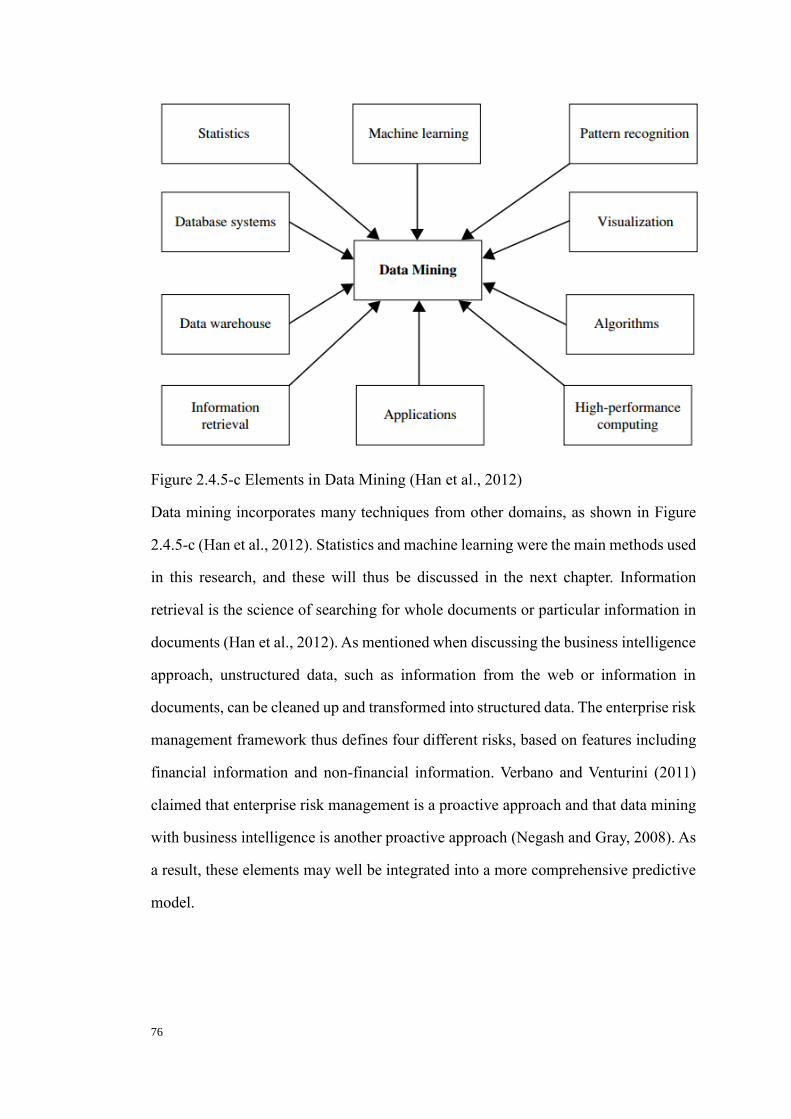
76
Figure 2.4.5-c Elements in Data Mining (Han et al., 2012)
Data mining incorporates many techniques from other domains, as shown in Figure
2.4.5-c (Han et al., 2012). Statistics and machine learning were the main methods used
in this research, and these will thus be discussed in the next chapter. Information
retrieval is the science of searching for whole documents or particular information in
documents (Han et al., 2012). As mentioned when discussing the business intelligence
approach, unstructured data, such as information from the web or information in
documents, can be cleaned up and transformed into structured data. The enterprise risk
management framework thus defines four different risks, based on features including
financial information and non-financial information. Verbano and Venturini (2011)
claimed that enterprise risk management is a proactive approach and that data mining
with business intelligence is another proactive approach (Negash and Gray, 2008). As
a result, these elements may well be integrated into a more comprehensive predictive
model.
77
2.5 Gap Analysis
As risk may bring both losses and gains, research on risk management is a highly
contentious issue. However, although a great deal of the literature shows an interest in
applying risk management in SMEs, the number of published papers remains limited,
which means that many areas are still understudied. Islam et al. (2006) claimed that
while many studies have been done on risk and risk management, most of them focus
on particular industrial contexts, and in particular on the industries associated with
safety and occupational health hazards. As a result, risk management in the SME
sectors has been given lower priority, as it is generally considered less catastrophic.
Risk management for SMEs requires the adoption of risk management strategy and
methodology, unlike risk management in larger organisations (Verbano and Verturini,
2013). Islam et al. (2006) also argued that the SMEs have specific limitations which
lead to their risk types and factors differing from those of other organisations, requiring
risk identification and categorisation to be developed specifically for this sector.
Verbano and Verturini (2013) argued that the tasks of risk management include
identifying risks, measuring the potential consequences of events, and reducing or
mitigating any possible loss. Vergas-Hernandez (2011) also claimed that SMEs needed
to obtain competitive advantages and succeed in the market by protecting their
innovative projects. Risk management in SMEs thus presents new challenges for
scholars, requiring more specific and systemic methods for risk identification,
evaluation, and treatment. The three mains steps mentioned previously as part of risk
management are called risk assessment in the ISO 31000 standard, and the elements
and factors in each step should be adjusted based on the features of SMEs to provide
more helpful information to decision makers. It has also been argued by Samani et al.
(2017) that the integration of the RM process with other processes or systems is
possible. It concluded that the three main steps in the risk management process could

78
be integrated with other process and components to improve efficiency and
effectiveness.
The data mining process provided a solution to the whole risk management process.
Johnson (2010) attempted to provide a conceptual mapping of risk management and
data mining. In Johnson’s study, he did not select a standard risk management process
like ISO 31000 standard. Also, he applied the Cross-Industry Standard Process
(CRISP) for the data mining process. However, compared with the data mining process
developed by Han et al. (2012), the CRISP-DM process does not show a significant
advantage in the whole process. On the other hand, the standard risk management by
ISO 31000 was widely used and mentioned by scholars (Verbano and Venturini, 2013;
Samani et al., 2017). Meanwhile, follow the ERM framework and risk management
process, the use of KRIs and KPIs mainly belongs to feature selection, which may not
require all the functions provided by the CRISP-DM process. According to Di Serio
et al. (2011), the risk management is a dynamic process, where the ‘monitor and
control’ step in ISO 31000 standard also required to adjust goals upon the need of
specific firms. The risk management process in this study will also be embedded with
other elements such as BI approach, EWS and ERM framework. Therefore, the
standard risk management process can be integrated with other processes more
effectively and efficiently, while the standardised data mining process is not suitable
for the risk management process in this study for SMEs.
The application of non-financial indicators presents new challenges. Altman et al.
(2010) studied the value of non-financial information in the prediction of SMEs;
however, although they used a combination of financial and non-financial indicators
in their models, the financial indicators were selected from their previous study, and
only five were used. Further, the performance of firms had already been decided by
the provider of the data. It could thus be concluded that that research did not follow

79
the whole procedure of risk management laid out by ISO 31000 standards or COSO.
According to Verbano and Venturini (2013), of the thirty-three relevant papers from
1999 to 2009, none covered all types of risks in a single piece of research, and only a
third of researchers covered the whole risk management process (identification,
evaluation, treatment, and context analysis). As risk management requires the adoption
of the whole process to support decision makers, it is necessary to create a model that
includes the processes mentioned in the ISO 31000 standards. The application of non-
financial indicators should not be solely instituted at the risk treatment step, but instead,
should be integrated into the whole risk management process. The current study's
application and integration of financial and non-financial indicators is thus an
innovative attempt to examine the risk management process.
Regarding risk assessment processes following ISO 31000 standards, several scholars
have studied these using their methods (Altman et al., 2010, Geng, Bose and Chen,
2015, Koyuncugil and Ozgulbas, 2012). Geng et al. (2015) stated that several
classification algorithms are available for financial distress prediction. In their
research, they compared four different algorithms to predict the distress of firms;
however, it was not possible to identify which algorithm provided the most accuracy
before a comparison of methods. If only one method were applied, there might thus
be a lack of evidence that the selected method was the most suitable and accurate
choice. Moreover, risk indicators may change over time, as they are determined by the
external and internal environments (COSO, 2003). It is thus not meaningful to use the
same indicators for varying time periods or countries, as the situations are different
and change over time. As each method uses different core algorithms, the results
should naturally be different, and the significant indicators may differ from one
method to another. Several methods should, therefore, be applied in the risk
assessment process to achieve more convincing results, and these methods should be
compared with each other to help select the most suitable.

80
Business intelligence provides a unique way of thinking about data analysis. Negash
(2004) defined business intelligence as “a system combined data gathering, data
storage, and knowledge management with analytical tools to present complex internal
and competitive information to planners and decision makers”. Comparing this with
the definition of the risk management process provided by ISO 31000 standards,
which includes establishing the context, risk assessment, and risk treatment, each risk
management process can be matched with business intelligence steps to a certain
extent. For example, when decision-makers need to establish context, they must
determine the purposes and objects of actions; data gathering, and data storage could
provide enough information to allow the decision makers or planners to ascertain
patterns or rules for specific groups. Business intelligence can thus convert data into
useful information, which people could use to develop knowledge (Negash, 2004).
According to Negash (2004), business intelligence makes use of both structured and
unstructured data, where the unstructured data is gathered from reports, research,
spreadsheet files, and so on. As discussed, this non-financial information and some
financial information can be classified as unstructured data. Thus, the use of business
intelligence approach can help the DM process, which also improves the risk
identification step in the risk management process.
The identification of KPIs and KRIs in SMEs is also a relatively new area. Scarlat et
al. (2012) stated that KPIs are focused on the historical performance of firms and their
key operations, while KRIs provide real-time information about future risks. The main
difference between KPIs and KRIs is thus that the former indicates whether goals are
achieved or not, while the latter explains the changes in risk profiles, the situation of
firms and the probability of achieving the target goals (Scarlat et al., 2012). As a result,
the key performance indicators should indicate whether the past performance of the
firm has been good or not. Davies et al. (2006) also pointed out that the key indicators

81
provide important information, serving this purpose very well. Based on this
characteristic, the key risk indicators should not be solely decided by decision makers
or management. Instead, the key risk indicators should be founded on rational and
logical algorithms, considering their importance, threshold values, significance, and
sequencing. Although Scarlat, Chirita and Bradea (2012) noted the importance of KPIs
and KRIs, they did not suggest a method of identification and classification of key
indicators. The resulting lack of procedures for the assessment of KPIs and KRIs thus
requires amendment; results will be more convincing where one or more sophisticated
algorithms guide the process.
There are thus several gaps in the existing research: the application of enterprise risk
frameworks in SMEs, the value of non-financial indicators in risk management in
SMEs, the selection of algorithms in risk assessment for SMEs, the method of
identification of KPIs and KRIs, and the use of business intelligence in risk
management in SMEs. Furthermore, the integration of the whole process within risk
management remains a challenge, as the risk management process is not a single-step
method. Following ISO 31000 standards helps to establish a more precise procedure
for management or decision makers, but the selection of algorithms is also an
important part of the risk management process, which requires efficiency and efficacy
(Scarlat et al., 2012). It is therefore clear that the challenges of risk management for
SMEs should be further studied, based on the existing framework and theories.
After reviewed existing literature, the current gap can be then identified. Firstly, the
integration of the DM process to the RM process is needed. Although Johnson (2010)
used the CRISP-DM process to a RM process, the RM process in his research is not a
standardised process. Gjerdrum and Peter (2011) thoroughly described the ISO 31000
and COSO ERM framework. They concluded that the ISO 31000 increased
‘accountability and strengthens communication’, which means the standardised RM

82
process has advantages. Therefore, the integration of the DM process to a standardised
RM process can increase the ability of SMEs to deal with potential risks. Secondly,
the BI approach has been used to visualise and quantities data for years (Nagash, 2004).
The BI approach can provide a general view of dataset from the beginning of the DM
process. It can also transfer non-numerical information into numerical format that can
be directly used as input data for the DM process. But the use of BI approach can
extract a high level of knowledge from raw data (Cortez and Silva, 2008). But the use
of BI approach with the DM process in the RM process is still a new area, which
requires more guidance on relevant theory and practice. Thirdly, the effectiveness of
ERM framework in the RM process should be examined. There are two components
in the ERM framework were used, which are risk types, KRIs and KPI (CAS, 2003).
The ERM framework is a holistic framework, which aims to capture both financial
and non-financial features from the risk management views. There are four different
risk types, which cover financial and non-financial features of firms. On the other hand,
the use of KPI and KRIs can reduce the number of indicators that the SMEs should
focus on. The SMEs can monitor KRIs rather than all indicators, since the other
indicators are not important as KRIs. The cost will be reduced, and the efficiency of
the RM process will be then increased. Fourthly, the EWS can be used in the risk
treatment step. The rules and pattern generated from the DM process can be analysed
in detail. The threshold value of KRIs and the importance of KRIs will be found out,
which provides explanations about the KRIs. Based on this information, it can know
how and why the risks affect firm performance. Fifthly, The Financial and Non-
financial factors have been used together in the DM process, which captured more
comprehensive features of the RM. In the other studies, the financial indicators have
been applied at the most time, while the use of non-financial indicators was only
suggested by many scholars (Altman, 2007). However, some scholars tried to find out
the value of non-financial indicators in relative topics (Altman et al., 2010; Geng et
al., 2015). In this study, there are more financial indicators have been considered and

83
included, which followed the risk catalogues of the ERM framework. Followed the
existing framework, the explanatory and meaningfulness of non-financial indicators
can be addressed and specified more clearly. As a result, through comparing prediction
accuracy of the data mining methods with different groups of financial and non-
financial indicators, the value of non-financial indicators can be shown directly.
Finally, the performance of DM methods in RM for SMEs will be compared. In the
RM process for SMEs, it is important to reduce the costs and increase accuracy. To
achieve these goals, the feature selection functions of DM methods will be mainly
considered. To evaluate the performance of DM methods, the prediction accuracy,
comprehensiveness of the results, and complexity of the methods will be compared.
The comparison of different DM methods has been applied in other studies (Geng et
al, 2015). However, the comparison of the methods (LR, CHAID, GA, BPNN) in this
study is a new set. Therefore, based on the evaluation of these four methods, it is
possible to find out the most suitable DM method for RM in SMEs.
2.6 Summary
In this chapter, general background to risk management was introduced. As the
development of risk management has occurred over only a few decades, the stages of
risk management are not yet mature. As Verbano and Venturini (2011) stated, there are
nine main paths of development in all the fields of risk management. The paths differ
from one another, and depend on the different approaches used, risks considered,
techniques and methodologies proposed, and fields of application. Therefore, if the
research target selected is enterprise risk management for SMEs, the corresponding
financial theories and tools for risk identification and assessment must be selected
(Verbano and Venturini, 2011). The ISO 31000 standard and COSO framework for
enterprise risk management were reviewed, and it was noted that enterprise risk
management considers all the risks suggested by CAS (2003), which is the most

84
holistic and integrated framework of the seven main risk management methods
(Verbano and Venturini, 2011). To identify the most accuracy and efficient risk
management method for SMEs, it is appropriate to use the enterprise risk management
framework, while to determine the correct risk management process for SMEs, it is
also important to introduce the background and definition of SMEs. Furthermore, the
application of enterprise risk management frameworks to SMEs is a new field, which
requires a careful selection of indicators and methods. Verbano and Venturini (2013)
pointed out that there were only thirty-three papers about risk management for SMEs
between 1999 and 2009, and that only fourteen out of the thirty-three papers used
enterprise risk management frameworks. Further, only one paper included more than
two risk types. Consequently, the framework of risk management processes for all
types of risks in SMEs requires an introduction and a more detailed discussion.

85
3. Development of the Theoretical Framework for
Risk Management in SMEs
3.1 Introduction
The previous chapter has reviewed the risk management process, risk management
framework and ERM framework, the related concepts of risk management and
identified the gaps in research, which is focusing on the risk management process, data
mining process and ERM framework. It emphasised the usage of non-financial
indicators and the solution of combining the data mining process and risk management
process. The purpose of this chapter is to develop a theoretical model for risk
management, which combined with the data mining process, ERM framework and BI
approach in order to address the purpose of this research.
The structure of this chapter is shown as followed. The Theoretical Background
discussed the frameworks in detail. After that, the components of the purposed
framework have been introduced. Then, the hypotheses are developed and justified
based on previous research.
3.2 Theoretical Background
Risk management in small and medium-sized enterprises has been less developed
because SMEs have a comparative lack of resources and reliable mechanisms
(Brustbauer, 2014). The risk management processes in SMEs are thus mainly based
on the perception of the owners rather than expert boards of directors as in large
companies (Herbane, 2010; Leopoulus, Kirytopoulos and Malandrakis, 2006; Nocco

86
and Stulz, 2006). In recent years, the overarching view of risk management has
changed from evaluating risks from an individual perspective to taking a more
generally encompassing perspective, which is also known as enterprise risk
management (Brustbauer, 2014). However, Florio and Leoni (2017) stated that the
empirical evidence on the relationship between ERM and performance is still limited.
Florio and Leoni (2017) argued that the reason for little empirical evidence is that it is
difficult to explain the relationship between ERM and firm performance. Verbano and
Venturini (2011) stated that ERM is the application of financial theories (Value
Maximisation and RM) and the adoption of tools for risk identification and risk
assessment, with the aim of maximising the firms’ value. Therefore, the risk
management process could combine with ERM framework to specify the risk
catalogues, reduce the impact of uncertainty and then increase the firms’ value.
In this section, the discussion will point out the theoretical foundations of this research.
This chapter was divided into subsections: the first one introduces the ERM
framework and risk management process. The second subsection focuses on the data
mining process and the combination of the data mining process and risk management
process. The third subsection describes the process of constructing the risk
management framework with ERM framework with all the components together. The
last one developed the hypotheses.
3.2.1 The ERM Framework
Enterprise risk management can increase risk management awareness by supporting a
firm-wide risk management approach, which translates more effectively into mature
operational and strategic management decisions (Nocco and Stulz, 2006). The
enterprise risk management framework provides general guidance and key principles,
leaving details to the individual firm (Brustbauer, 2014); even the definitions of risks

87
may thus be different. However, the general agreement about risks in recent years is
that the risks include both downside effects and positive effects. As defined by COSO
(2017), enterprise risk management is a process that it is effected by an entity’s board
of directors, management, and other personnel, applied in both strategy setting and
across the enterprise, that is designed to identify potential events that may affect the
entity and thus manage risk such that it remains within the entity's risk appetite, thus
providing reasonable assurance of the achievement of objectives. Pagach and Warr
(2011) stated that the enterprise risk management framework aims to identify, assess,
and monitor all threats and opportunities faced by the firms. As mentioned in Chapter
2, there are four main kinds of risks faced by SMEs under the ERM framework: hazard
risk, operational risk, financial risk, and strategic risk. In many studies, scholars have
constructed models to predict company performance by analysing financial ratios
(Altman and Sabato, 2007; Altman et al., 2010; Lussier and Pfeifer, 2001). It can be
concluded, however, that the risks faced by companies can be monitored more
effectively using the changes in both financial ratios and non-financial ratios. To
systematically manage different risks, this research will thus adopt existing developed
frameworks and add additional variables to explain the risks and thus improve the
efficiency of risk assessment and monitoring procedures.
As Verbano and Venturini (2011) stated, ERM is an extension of financial risk
management (FRM) to non-financial circumstances, where the non-financial part is
not studied as much as the financial part. Beaver (1967) and Altman (1968) first
applied financial ratios to building business failure prediction models, while Nocco
and Stulz (2006) found that financial risk management and firm value are correlated.
Chen et al. (2010) applied a KMV model in the analysis of credit risk, and Wu and
Olson (2009) demonstrated validation of predictive scorecards for large bank risk
management. However, none of these previous studies provided a holistic and
integrated model in the term of all risks. Verbano and Venturini (2013) stated that

88
integrated risk management (also called enterprise risk management or holistic risk
management) began in 2000 as an approach to align strategy, processes, people,
technology, and knowledge with the process of evaluating and managing risks (threats
and opportunities) (De Loach, 2000). Verbano and Venturini (2013) also stated that
this required a re-ordering of the risk management discipline into a single framework
to identify and characterise the different approaches to risk management. Based on
this complete framework, future scholars would then be able to pool knowledge
accumulated from individual development experiences (Verbano and Venturini, 2013).
Verbano and Venturini (2013) also pointed out that the ERM is the most studied
framework since it covers all risk types. Enterprise risk management framework
adopts the tools for risk identification and assessment to maximise the expected value
of a firm; there are thus many advantages of applying an enterprise risk management
framework in the risk management process. Several organisations also provide
frameworks to help risk management, including COSO, ISO, and CAS. However, in
the past, only a few researchers, such as Fraser and Simkins (2016) and Bromiley et
al. (2014), focused on the usefulness of enterprise risk management in companies.
According to many scholars (Lam, 2001; Liebenberg and Hoyt, 2003), enterprise risk
management framework provides a higher probability of reaching a firm's goals; a
reduction in the cost of capital; a greater understanding of the main risks; optimisation
of the portfolio of risks; a reduction in the volatility of cash flows; a definition for
intervention priorities; improvement in compliance to norms; a smaller number of
unforeseen events and consequent losses; a more significant push for change; greater
response speeds to varying business conditions; and a greater tendency to accept risk
in order to gain higher returns (Verbano and Venturini, 2013).
Key performance indicators (KPIs) and key risk indicators (KRIs) can be identified
and monitored more efficiently by integrating the four major types of risks into one

89
complete framework in order to improve the prediction of business failure and to
detect potential risks. The KPIs are used to measure firms’ performance, which
allowed the firms to set goals on performance (Delcea et al., 2013). The KRIs can
provide information about unfavourable trends (Delcea et al., 2013). Delcea et al.
(2013) also mentioned using EWS to monitor KRIs to control risks. CAS (2003) also
stated the KPIs and risks are linked to the ERM framework. Keith (2014) also pointed
out that the ERM framework linked KPIs and KRIs to manage the risks effectively.
The risk management process could be simplified to control KPI and KRIs instead of
considering and monitoring all indicators. Therefore, the application of ERM
framework in the risk management process could provide an integrated view, which
may also improve the efficiency of the whole risk management process.
Many scholars have studied risk management in different aspects, including its
elements, steps, methods, and so on. Kloman (1976) started such research with “The
Risk Management Revolution”, and many practitioners have since advocated a
coordinated approach to risk management. Kloman (1992) described the concepts
coming out of Europe from the mid-'70s to the early '80s, with theory now associated
with ERM. Gustav Hamilton, a risk manager in Sweden, argued for “a new and
collective view of risks” (Kloman, 1992). Kloman (1992) also argued that the elements
of risk management for enterprises must be based on the enterprise being treated as a
system. The process of risk management in enterprises could thus be considered as a
kind of information system. In such a system, the risk managers need to keep sending
risk and uncertainty information from enterprise to managers and other departments
to deal with future risk. Gleason (1999) stated that the risk management process
includes the processes of identifying, measuring, and solving. Initially, it is imperative
to measure the risks faced by the firm, and after this risk measurement, a process for
evaluating the impacts of those risks should be applied. It is also important to set up
a department to manage and control risk and to evaluate the potential loss inherent in

90
any risk accepted.
Figure 3.2.1-a The Risk management cycle with ERM (Source: Keith (2014))
The five steps required by ISO standards are thus accomplished within the framework
(Keith, 2014). As shown in Figure 3.2.1 a, the external environment mainly affects
only the first step of the framework, while the ensuing four steps are closely linked
with the internal environment. The most important elements in the internal
environment are the key risk indicators and key performance indicators. The KRIs and
KPIs build links between risk identification, risk assessment, and risk response steps,
and these three steps are the main processes in the ISO framework, collectively known
as the risk assessment phase. Keith (2014) argued that KPIs and KRIs work
simultaneously in the enterprise risk management framework, interacting with risk
identification risk assessment and risk response. However, these risks could thus be
only identified after firms have been affected; meaning that KPIs can be considered
ineffective, as they measure events that have already happened, and which have thus
already had an impact on the enterprise’s performance (Kaplan, 2009). The key
performance indicators can be used to see whether performance has been achieved or
not, while key risk indicators can indicate how the risk profile has changed within

91
desired tolerance levels. Thus, while KPIs provide information about past events,
KRIs can thus potentially provide insights into future potential risk events (Taylor and
Davies, 2003). For example, performance metrics can be used to measure expected
performance, and KRIs can predict the downside risk or volatility of such performance
(Smart and Creelman, 2009).
KRIs play critical roles in the whole risk management process. For instance, if
organisations use self-assessment tools for risk identification and control, KRIs can
facilitate the monitoring process at set intervals. They can also indicate what the
entity's risk appetite is (Immaneni et al. 2004). When used appropriately, these tools
can provide the insight needed to track business strategies and thus drive through the
benefits of change (Kaplan and Norton, 1992; Frigo 2002). Developing a set of
effective KRIs should, therefore, enable managers to identify relevant measures. It can
also provide information about the impact of risks on the accomplishment of target
objectives. Based on this, developing a good understanding of target objectives is more
important than creating enterprise-wide KRIs, though developing effective KRIs is
treated as the most important process in most organisations. Financial organisations
usually focus on indicators of credit risk and market risk (Lam, 2005), and thus some
of them may be challenged when required to develop KRIs for financial risk,
technology risk, or operational risk.
Lam (2003) stated that KPIs could be developed from various sources such as policies
and regulations, strategies and objectives, previous losses and incidents, stakeholder
requirements, and risk assessments. According to Immaneni et al. (2004), there are
two approaches to effectively addressing KPIs, which are top-down or bottom-up. The
top-down method assesses general objectives and risks, then designs appropriate risk
indicators. In contrast, the bottom-up approach defines specific processes and risks.
Some unique business areas may be better suited to the bottom-up approach; for

92
example, where there are special requirements in some corporations, the bottom-up
approach could provide more accurate information on targeting objectives, which
could be used to develop unique KRIs based on those unique corporate environments.
One proposed way to overcome this challenge in other cases is to select measures that
edge over the limit and to transform them into an index that acts as a tool to merge
findings from different indicators and report them in aggregate (Immaneni et al., 2004).
Figure 3.2.1-b The Use of KRIs (Immaneni et al., 2004; Keith, 2014)
The objective of KRIs is to create a better business performance. Thus, management
will always set goals to increase profitability. An entity can either increase revenues
or reduce costs to increase revenue. If firms want to achieve these two different results,
different strategies must be applied, and whenever strategies are set to achieve target
goals, these may come with potential risks. As stated in COSO 2010, potential risks
can be highlighted and mapped to core strategic initiatives so that management can
create metrics to contribute most effectively to the execution of the strategic goal. As
the framework represents a dynamic process, continuous monitoring and analysis of
internal and external environmental changes are also important. The framework thus
demonstrates that the use of KRIs and KPIs can enhance monitoring and control risk
to achieve target objectives (COSO, 2010).

93
3.2.2 The Risk Management Process
The risk management follows a stage-gate process (Verbano and Venturini, 2013). The
process of risk management is thus shown in Figure 3.2.2 below:
Figure 3.2.2 ISO standard risk management process (ISO 31000, 2009)
There are total of three main parts of the risk management process, which are Establish
the Context, Risk Assessment and Risk Treatment. Additionally, the Risk Assessment
part contains three sub-steps, which are Risk Identification, Risk Analysis and Risk
Evaluation. Meanwhile, the Communication and Consultation step and Monitor and
Review step will constantly interact with all other steps to control the quality of the
risk management. The most important step is the Risk Assessment, which contains
three sub-steps (Verbano and Venturini, 2013). They stated that the first sub-step aims
to identify all the risks that the firms faced. The second sub-step aims to determine the
probability and magnitude of the potential damage. The third substep is to identify the
most suitable actions to reduce the effect of risk. The whole risk management process
is a long-term, dynamic and interactive process (Di Serio et al., 2011). As a result, a
process that considers all the steps and complies with long-term, dynamic and
interactive is ideal for the risk management process.
During daily activities, enterprises may realise they will face future risks. However, it

94
is not easy for them to identify what kind of risks and how those risks will affect their
operational activities. There might be many indicators under each risk category, and
these the indicators may or may not be related to firm performance. This makes it
important to uncover these risks and to figure out how to assess them effectively. The
biggest issue is to identify the firm's performance at the very beginning, which makes
the risk management process more difficult. It is also necessary to identify one or more
key performance indicators (KPIs) to measure the firm's performance, which should
be readily comparable and allow classification of firms into different groups. So that
firms can be classified, it has been assumed that the performance of firms differs and
that selected KPIs can explain these differences. Based on these different performance
levels, it would thus be possible to identify the risk indicators adopted by annual
reports and government institutions. Risk indicators could also be classified by types
of risk under the enterprise risk management framework created by CAS (2003). This
makes it possible to identify key risk indicators under four risk categories. If these key
risk indicators are confirmed, the risks can be ranked, evaluated, and explained by
management in many different ways. The risks faced by SMEs have unique features,
which are not same as in other sizes of the enterprise; thus, to assess these risks, it is
important to discover directly effective methods rather than using universal methods.
Unique threshold values, road maps, classifications and sequencing must thus be used
to capture the features of SMEs, which should also guide decision makers. More
specifically, decision-makers can use those methods to build an early warning system
to control the risks and improve performance.
The risk assessment process can thus be explained as follow. Before any risk
assessment steps, the performance of the firm should be assessed from the data sets.
Delcea et al. (2013) stated that enterprise performance could be measured by using
key performance indicators (KPIs). They also noted that the Risk Management
Associations (RMA) had developed a project about Key Risk Indicators (KRIs) that

95
can be helpful regarding accessing, measuring, and controlling different types of risks.
Enterprise performance is most generally reflected in financial status, and based on
the information provided by KPIs; it is possible to set objectives and monitor progress
within a reasonable interval. Taylor et al. (2008) mentioned that enterprises could also
monitor and predict the value of key performance indicators using a simulation tool.
However, since the purposes of KPIs and KRIs are different, there might be conflicts
in setting KPIs and KRIs. The risks faced by each company are different, and every
company has its unique focus on risk management. Once again, it should be
emphasised that KPIs and KRIs must not be confused with each other, and the
application of KPIs should come before the identification of KRIs. Risks may affect
the performance of firms, which indicates that risks can, therefore, be identified by
comparing the performance of different firms.
As there are four different types of risks, and each different display characteristics, it
becomes necessary to treat different risks separately; KRIs and KPIs are both
important in this risk management process. KRIs, for example, can be used to detect
unfavourable trends (Delcea et al., 2013). The risk identification step should come first,
to classify the different risks. In the risk identification phase, the problems faced by
companies can be classified using the four major risk types to help them focus the
problems more efficiently. For example, where companies find that financial problems
are the main issue, it is likely that financial risk has existed and not been treated in the
past.
When a company is expanding, its operations and progress become more complex,
and within these more complicated situations, the potential risks also grow. Risk
indicators at that point could be either financial or non-financial, but Altman et al.
(2010) argued that using non-financial variables could improve the accuracy of
predicting company failure. Islam et al. (2006) agreed that the indicators could be

96
financial or non-financial depending on the problems to be solved. For example, if
decision makers want to know the financial situation of a firm, the most direct form
of measurement is financial ratios, while if they need to measure other information,
such as industry, employee education, or audit information, the non-financial
indicators could more directly indicate this kind of information. Both financial and
non-financial indicators can be integrated into a combined model as risk indicators,
where they can be filtered and treated via business intelligence tools to determine key
risk indicators. It is important to reassess and measure key risk indicators regularly in
order to detect risks before they become harmful. Whenever one or more variables
meet the thresholds set, it is possible that the company will be affected by future risks.
KPIs are also important in the risk management process, and thus if enterprises set
their goals and define their risk requirements, both KPIs and KRIs can be appropriately
used in risk analysis progress. Although KPIs and KRIs are helpful in the risk
management process, the application is still needed to be specified and optimised.
3.2.3 The Early Warning System
Based on the different types of risks, it is possible to evaluate most enterprise situations
and to use key risk indicators to set up an early warning system, which could be useful
to Risk Evaluation step. According to Bussiere and Franzscher (2006), early warning
systems are developed to detect underlying economic weaknesses and vulnerabilities;
furthermore, an early warning system can make it possible to reduce risks before a
crisis by allowing management to take some pre-emptive steps. Koyuncugil and
Ozgulbas (2012) defined an early warning system as an analysis technique used to
predict the achievement conditions of enterprises and to decrease their risk of the
financial crisis. It is thus apparent that KPIs and KRIs can be adequately fitted within
early warning systems. Koyuncugil and Ozgulbas (2009) noted that a good early

97
warning system can provide identification of changes in environment; identification
of speed and direction of changes projected into the future; identification of the
importance of the degree of changes; determination of deviations and signals;
determination of possible reactions in the direction of privileged deviations; and
investigation of the factors which cause changes and transactions between these
factors. Such an early warning system is the type of predictive model, offering the
chance to take corrective precautions in the long-term (Koyuncugil and Ozgulbas,
2009). An early warning system based on financial ratios could predict the profits of
firms, potential bankruptcy risks, and any impending crisis for enterprises' economic
trends. More importantly, it could make use of KRIs and KPI to increase the efficiency
of the RM process.
The application of early warning systems is complicated. As Koyuncugil and Ozgulbas
(2009) noted, financial early warning systems are based on financial ratio analysis. In
these financial ratio based systems, administrative and structural factors are ignored,
as are human factors. Thus, financial early warning system does not consider all of the
relevant variables, which may lead to bias in the results. Striving to complete and
improve on the application of early warning systems, many scholars have contributed
studies on the use of early warning systems. Canbas, Cabuk, and Kilic (2005) created
an integrated early warning system by combining three parametric models based on
the principal component analysis (PCA). Oh, Kim, Lee, and Lee (2005) further stated
that it is important to establish an alarm zone to predict potential crises. The basic
process of establishing an early warning system is shown in Figure 3.2.3:

98
Figure 3.2.3 The Process of establishing EWS
Firstly, the firms should be classified into two groups based on the KPI, which
indicates the performance of firms. The target Canbas et al. (2005) pointed out that, in
bank failure studies, banks were split into two different groups: healthy and failed.
Thus, to establish an early warning system for SMEs, it is important to classify the
enterprises into two or more different groups, where the features of indicators could
be studied. Based on the classification results, different sets of characteristics can then
be generated in order to uncover the differences between groups. It is also necessary
to define the standards of good and poor performance. Secondly, the most important
step in this system is the generation of characteristics, as the conditions and thresholds
defined later are based on the results of this step. Thus, to obtain more accurate results,
it is necessary to apply more than one data mining method in the selection of KRIs.
Furthermore, the focuses and process of each data mining method are not the same,
where using more methods may provide more comprehensive views of KRIs. Finally,
the Rules and Patterns are explored by evaluating KRIs. The KRIs will be deeply
analysed in order to generalise the ranges and significances of them, which will help
the decision makers to focus on fewer indicators. Since the early warning system starts
with the firms’ performance, the aim of the early warning system and risk management
process could be synchronised. As a result, the early warning system could increase
the efficiency of the risk management process, especially for Risk Evaluation step.

99
After generating characteristics, the groups of sample data can be classified clearly.
The characteristics of poorly performing enterprises may then indicate why they have
been classified into this group. The classification of different risks was discussed in
chapter two, and following categorisation into the four different risk types, it is
possible to uncover the thresholds between high-performance enterprises and poor
performance enterprises. These thresholds can be defined by using one or more
variables above or below pre-set values. It may also be much easier to generate
patterns of financial ratios and non-financial ratios from one of the groups. Based on
these patterns, it is possible to uncover the influences of different risks and to
determine the most important risk-related ratios. After this, the weights and
independent variables should be optimised based on the results of the previous steps.
For example, if the financial risk is the most significant risk, it is necessary to increase
the weight of the financial risk related ratios, so that these ratios will play more
important roles in the model and other, less significant, variables will take on less
weight.
Setting up an early warning system also requires defining the desired values. To
understand the performance of enterprises, examining examples of poor performance
could be helpful to identify the risks and the weakness of an enterprise. In contrast,
defining and identifying the desired values could be also helpful in understanding the
good performance and the achievement of objectives for enterprises. Any indicator
exceeding or missing a specified threshold value could thus be interpreted as a signal.
There are many signals amongst the ratio analysis results of most enterprises. If these
signals indicate that the enterprise is performing well, these signals could be adopted
into desired variables. On the other hand, if the signals indicate that the enterprise is
performing poorly or getting into financial distress, these signals should be taken as
warning signals. In high-performance groups, the desired variables will thus outweigh

100
warning signals. The features of different types of risks could also be identified during
this process, and the weights of different risks in different groups ascertained. For
instance, the sequencing could provide the rank of risk importance. As a result,
warning signals based on the various risk categories can be created within the early
warning system, making it possible to build integrated models, which indicate a range
of potential risks for enterprises. Such integrated models can allow enterprises to
improve their performance purposively, tactically setting their objectives to focus on
the improvement of one or more targets.
3.2.4 The Data Mining Process
This research used data mining theory to build models and select methods for the risk
management process. Soman, Diwakar, and Ajay (2009) pointed out that data mining
algorithms are included in the knowledge discovery in databases (KDD). A data
mining system allows users of databases to discover new knowledge from the data
(Adriaans and Zantinge, 1996). Some data mining algorithms use statistical methods,
but in essence, data mining refers to any means of discovering patterns within and
extracting hypotheses from the data. Soman et al. (2009) also stated that the data
mining differs from the traditional statistics in that data mining is used to extract
qualitative models using logical rules or visual representations. Rokach and Maimon
(2014) further noted that data mining is a term which describes the process of sifting
through large databases in search of interesting, previously unidentified patterns. Data
mining thus can make predictions about specific phenomena, and Soman et al. (2009)
argued that data mining is a part of the KDD process, providing algorithms to support
the overall KDD process.
Rokach and Maimon (2014) stated that data mining describes the process of finding
unknown patterns through large databases; it is the accessibility and abundance of data

101
that makes data mining possible. Data mining is also part of the Knowledge Discovery
in Database (KDD) process, which is shown in Figure 3.2.4:
Figure 3.2.4 Data mining Steps (Rokach and Maimon, 2014)
Rokach and Maimon (2014) defined the KDD process, including the data mining
process, as choosing the appropriate data mining task; choosing the data mining
algorithm, and employing the Data Mining algorithm. Figure 3.2.4 also shows the
steps taken to prepare data for mining, as well as showing how the data is transferred
to knowledge. Han and Kamber (2001) pointed out that many people treat data mining
as identical to KDD; they also stated that the data mining is often used to refer to the
entire KDD process in the industry, media, and research milieus. Soman et al (2009)
reaffirmed the four steps of the data mining process as data selection, data
transformation, mining the data, and interpreting the results, while Han, Kamber, and
Pei (2012) argued that there are seven steps to KDD, which are data cleaning; data
integration; data selection; data transformation; data mining; pattern evaluation, and
knowledge presentation. They also pointed out that the first four steps refer to different
forms of data processing, which prepare the data for mining. The data mining step is
the essential process, where intelligent methods are applied to extract data patterns
(Han et al., 2012), and the final two steps identify the patterns and present knowledge
102
to users. This affirms that the data mining process aims to uncover useful information
from large datasets which can then be applied to risk management procedures to
uncover potential risk factors.
3.2.4.1 Business Intelligence
BI approach could provide many helpful functions regarding ERM framework and
data mining process. McBride (2014) stated that BI provides the information and tools
for statistical analysis of large-scale trends, which also includes detailed characters.
McBride (2014) also pointed out that the KPIs could be examined and monitored at
every point, which is also complied with the risk management process. Han et al. (2012)
also stated that the BI approach provides reporting, business performance management,
benchmarking, and so on. The data collection is the basic step in the data mining
process, which will construct the database. The BI approach could support the
construction of data base by using software to collect the data from websites (Chen et
al., 2010; Han et al., 2012). Additionally, the BI approach also includes data cleaning
and arranging functions (McBride, 2014). It is evident that the whole data mining
process could be supported by using the BI approach. Moreover, the ERM framework
required both financial information and non-financial information to cover all four risk
types. It is important to collect information from any possible resources. As a result,
the database could be built by using BI approach in the data mining process.
Business intelligence can help decision makers to make decisions through the
application of both structured and unstructured data (Negash, 2004). Structured data
includes information from data warehouses, data mining, executive information
systems, online analytic processing, and enterprise requirement planning, while
unstructured data may include conversations, graphics, images, movies, news, and
web pages. BI converts data into useful information, which helps to transform the data

103
into knowledge using human analysis (Negash, 2004). The listed firms provide annual
reports to the public, which contains the balance sheet, cash flow sheet and other
related information (CFA, 2015). The financial information is more accessible to
collect than non-financial information, where the financial indicators could be directly
calculated by information in the balance sheet and cash flow sheet. However, the non-
financial indicators required to be cleaned and standardised before applied in data
mining methods, which should also be complied with the risk features under the ERM
framework. As a result, it is necessary to use the BI approach to generate financial and
non-financial information in order to use them in the data mining process.
The application of BI approach in data collection and data cleaning is very important
in this research. By using BI approach, it is possible to select any available resources
According to Tutunea and Rus (2012), BI in SMEs is variously perceived. Tutunea
and Rus (2012) noted that the BI solutions and products include dashboards,
localisation and business data visualisation, what-if analysis, interactive reports, and
readily interpretable formats for users. The most important part of BI in this research
is in the data collection and data cleaning steps. The SMEs required different focuses
on risk management (Kim and Vonortas, 2014). As a result, the BI approach may
provide more flexible adjustments, which could also dynamically adjusted (Chen et
al., 2010). The BI approach is also helpful in other parts of the data mining process.
For example, ‘mining the data’ and ‘rules and patterns’ may require BI approach to
provide classification and clustering. Specifically, data mining is the core of BI (Han
et al., 2012). Therefore, it would be helpful to use the BI approach in the whole data
mining process to provide support for most steps in the model.
3.3 The Conceptual Model
As discussed earlier, the conceptual model for this research includes the risk

104
management process, the data mining process, which also adopts the ERM framework,
EWS and BI approach.
Following the risk management process in ISO 31000 (2009), risk management is a
stage gate process (Henschel, 2009; ISO 31000, 2009) described in Figure 3.3-a:
Figure 3.3-a The Detailed RM process
The purpose of RM should be recognised in the “Establish the Context” step (Verbano
and Venturini, 2013) before the three sub-steps in the risk assessment phase are
completed. In the risk identification step, the risk should be thoroughly investigated
regarding what, how, when, and why risk may occur. The risk analysis is the most
complicated section of the risk assessment step and should provide a generally
complete understanding of each risk, the consequences of those risks, and the
likelihood of those consequences. Finally, the risk treatment phase provides possible
solutions and improvements for the firms concerned. It is possible to conclude that
data mining steps can be used to support the risk management process naturally by
combining this risk management process with a data mining process. For example, the
Establish the Context process specifies the purposes of risk management, making it
important to decide the KPIs and KRIs at this stage; this can be related to the data

105
selection step in the data mining process.
Similarly, in the risk assessment step, the target risks should be analysed and explained
in detail; the data transformation and mining the data stages of the data mining process
can thus provide theoretical and practical support for these stages, including selecting
and transforming appropriate information to create risk indicators. Further, based on
the interpretation stage of the results of the data mining process, decision makers could
decide on the actions to be used in the risk treatment step of the risk management
process. In this way, it is possible to use data mining methods in the risk management
process to achieve risk management goals.
The data mining process includes four steps: data selection; data transformation;
mining the data and interpretation of results (Soman et al., 2009). The most important
part of this process is data selection, which provides the resource for the ensuing steps.
Soman et al. (2009) stated that the variables selected, and the range of the data to be
examined should be specified in this step before data transformation is used to shift
the data into the particular formats required by the chosen data mining tools. After that,
the data is analysed using those data mining tools, and the results of the data analysis
represented numerically or visually. The data mining process is not a one-step process,
making it similar to the risk management process as outlined in ISO 31000.

106
Figure 3.3-b Flowcharts of DM-RM model
Figure 3.3-b shows the combination of risk management procedures with a business
intelligence approach in an enterprise risk management framework in the flowchart.
The data mining process and risk management process are combined via KRIs and
KPIs. As the purpose of the risk management process and data mining are similar, it
is possible to combine the two processes to achieve risk management goals. The two
frameworks can be connected by using KPIs and KRIs, where the KPIs provide a
measurement of purposes or goals and the KRIs provide insight into rules and patterns.
Also, the business intelligence approach supports the use of information from
databases, data warehouses, the internet, and other information repositories. While the
information collected from the internet or other external information repositories may
not be basic forms of data (Han, Kamber and Pei, 2012), these non-basic forms can be
transferred into basic forms of data to be used in the data mining process.

107
Figure 3.3-c The Research Conceptual model
Figure 3.3-c shows the conceptual model of this research. The model indicates the idea
of combining the data mining process to the risk management process, which also
considers enterprise risk management (ERM), early warning system (EWS), business
intelligence (BI). Also, the research objectives are selected as SMEs. The RM process
is a stage gate-process, which includes three main steps (Verbano and Venturini, 2013).
The data mining process could also be presented as a stage-gate process. It is possible
to combine two processes in one model, which could achieve risk management goals
by using the data mining process. Han et al. (2012) defined data mining is: “the process
of discovering interesting patterns and knowledge from a large amount of data”.
Therefore, in the data mining process, the data is the most important component. The
data mining process also includes several steps, such as four steps by Soman et al.
(2009) and seven steps by Han et al. (2012).
The ERM, EWS, BI will support the data mining process by providing guidance on
data selection, data collection and data analysis for SMEs. Since these systems or
models cannot be directly applied in the model, it is necessary to introduce the
mediators to link them together. Initially, the information provided by firms and
government or other institutions will be transferred into the indicator format. The BI

108
approach can collect the data and clean the data by using Web clawer, classification
tools, etc. The listed Chinese SMEs were selected as research targets, where the annual
reports were downloaded by using Web claws and the useful information are generated
and cleaned by using classification tools. The ERM provided risk catalogues, which
includes four different risk types (CAS, 2003). The indicators can explain the risk
features defined by the ERM. As many scholars emphasised the importance of non-
financial indicators (Altman et al., 2010; Geng et al., 2015; Li et al., 2017; Koyuncugil
and Ozgulbas, 2012), the indicators were classified as Financial Indicators (FIs) and
Non-Financial Indicators (Non-FIs) in this research. Then, these indicators will be
used as candidates of KPIs and KRIs based on the ERM framework, which provides
the linkage between the components shown in Figure 3.3-c. After that, the KPIs and
KRIs could be used as input data to the data mining process and risk management
process, where KPIs and KRIs will link each component of the two processes. The
EWS will use the rules and patterns of KRIs and KPIs to achieve the goals of the risk
management process by providing threshold values, risk sequencing, etc. Based on the
results of EWS, the warning signals and desirable trends can be found out, which will
support the decision-making. As a result, the data mining process has been
supplemented by many components to fit in the risk management process. The data
mining process will be discussed in the rest of this section, where the steps in the
process will be explained. Therefore, the developed model is called DM (Data Mining)
-RM (Risk Management) model in the following parts of this research.
The enterprise risk management framework can work throughout the whole model.
Based on the risk categories provided by CAS (2003), risks are divided into four
different groups, which guide capturing the features of each risk. As a result, the data
selection step follows the enterprise risk management framework, while it also
supports the risk identification step. The transferred data can then be used in the
mining the data and model and patterns steps to identify KRIs among all risk indicators.

109
All of the basic form data and non-basic form data can be used as risk indicators, and
the model and patterns step identifies the rules and patterns behind that data. The
patterns identified are based on the needs of the risk management procedure, though
the purposes of the two processes may be the same. As these patterns can be used as
thresholds, ranges, or other descriptors of KRIs, the risk evaluation and risk treatment
processes focus on dealing with these KRIs. Thus, problems are simplified by
identifying KPIs and KRIs for risk management.
Soman et al. (2009) stated that there are many classes of tools that can be used in data
mining processes, including Associations; Sequential patterns; Classifiers/Regression
analysis; Decision trees, Clustering; Data transformation and cleaning; Estimation and
forecasting; and Statistical analysis. According to the stage gate processes defined by
Henschel (2009) and ISO 31000 (2009), the entire risk management process may
require more than one method to achieve risk management goals. For instance, at the
beginning of the RM process, the decision makers may not know what the future risks
are precise. They must, therefore, identify potential risk factors and find out how to
detect risks before those risks become harmful to their firms. At that point, associations,
clustering, and classifier analysis could support decision-makers in the identification
of risk indicators and performance indicators for potential risks, while other tools
could be used to provide solutions for the on-going process of risk management.
Estimation and forecasting could provide prediction accuracy for the applied models,
and based on statistical analysis; the most important indicators could be selected for
observation to improve the efficiency of the decision-making process. The decision
makers could also generate patterns and rules in order to control KRIs to facilitate risk
reduction. In this way, data mining tools could be helpful throughout the risk
management process.
Data collection is one of the most important stages in data analysis (Rokach and

110
Maimon, 2014). Soman et al. (2009) pointed out that there are several research
challenges in the data mining process, which include improving the scalability of data
mining algorithms, mining non-vector data, mining distributed data, improving the
ease of use of data mining systems and environments, and privacy and security issues.
In the risk management process, the risk analysis part of the risk assessment step
requires decision makers to focus on dealing with data. Soman et al. (2009) stated that
information could be generalised into different types of data. Klieštik, Kočišová, and
Mišanková(2015) also argued that there are several different types of classification
variables: nominal variable, ordinal variable, interval variable, and ratio variable.
Nominal variables are quantitative, and cannot be identified into certain categories,
but only expressed by words or numerical codes (Kliestik et al., 2015). These include
the names of people or the names of places, which can be expressed as numerical
codes (such as 1, 2…, n) in modelling. Ordinal variables can be rationally listed in
some order (Soman et al., 2009) and included all the features required from nominal
variables (Kliestik et al., 2015). For example, the educational background of
employees is an ordinal variable, as it follows a set of levels such as primary, college,
masters, and so on. However, while it is clear that the master's degree is higher than
the college education, the ordinal listing does not specify how much higher. An
interval variable could be used to define the quantified difference between them
(Kliestik et al., 2015); however, this type of quantified difference may be arbitrary
(Soman et al., 2009). Taking temperature as an example, while 10 degrees is higher
than 0 degrees, 10 degree is not 10 times higher than 0 degrees. Ratio variables are
defined based on a "rational zero", which means that ratio variables have a true zero
point (Kliestik et al., 2015; Soman et al., 2009). Ratio variables can thus demonstrate
how many times one variable is higher or lower than another (Kliestik et al., 2015).
Mass is a ratio variable, as 100 kg is two times as massive as 50 kg.
In the data sets used in risk management processes, all the financial indicators are ratio

111
variables, such as quick ratio and net profit margin. Some non-financial indicators are
nominal variables, such as the names of provinces and audit opinions, while some are
ordinal variables, such as the educational background of employees. As most models
required input variables to be ratio variables, it is essential to quantise and standardise
the information into indicators. Data transformation steps thus play an important role
in both data mining and risk management processes.
In the ‘mining the data’ and ‘interpretation of results’ steps, data mining methods are
used to select KRIs, generate rules and develop roadmaps. The CHAID and Logit
regressions were used in this research, based on statistical probability theory (Geng et
al., 2015). The CHAID was developed by Kass (1980), based on AID (automatic
interaction detection). The CHAID utilises a nominal scaled dependent variable, with
an applied chi-squared statistic at each node (Kass, 1980). CHAID also reduces the
operative difficulty for inexperienced researchers due to its significance testing
framework. By using the significance of a statistical test as a criterion, CHAID can
evaluate all of the potential predictors (IBM, 2011). It can then merge all the values,
making them statistically homogeneous with the chosen dependent variable and
distinguishing all the different values to create branches. As the tree is grown based
on statistical testing, CHAID is thus based on statistical probability theory.
The Logit regression model is a well-established statistical method for the prediction
of binomial or multinomial outcomes (IBM, 2011). The Logit regression was used for
the selection of KRIs in this study, to provide a binary classification based on the
performance of firms (good or poor). The model assumed a dichotomous dependent
variable with a probability dependent on the weighted independent variables. For the
selection of KRIs, the likelihood ratio statistic was used to determine whether a
variable should be included in the model or not. The likelihood ratio statistic is defined
as two times the log of the ratio of the likelihood functions of the two models evaluated

112
at maximum likelihood estimates. The likelihood ratio statistic is asymptotically Chi-
square distributed with a degree of freedom equal to the difference between the
numbers of estimated parameters in the two models (IBM, 2011). Akaike (1987) stated
that the minimum AIC represents the best fit among models; as a result, the Logit
regression for selection of KRIs is a process of identifying the minimum AIC among
different combinations of indicators applied in the Logit, regression model. As both
CHAID and Logit regression apply statistical probability theory in their inner
algorithms, it is important to consider the threshold value of such statistical tests long
side other parameters.
As well as statistical methods, several other methods have been popular in addressing
similar problems in risk management. Artificial Neural Networks (ANN or NN) and
Genetic algorithms are also commonly used in data mining (Koyuncugil and Ozgulbus,
2012). An ANN is a non-linear predictive model that mimics the impulses from
biological neural networks. An ANN thus consists of a large number of "neurons" and
connections between those neurons, where the weights of factors are associated with
neurons (Back, Laitinen, and Sere, 1996). The weights can then be optimised for
certain outputs using a learning process. Genetic Algorithms simulate the Darwinian
evolutionary process. The algorithm defines a fitness value regarding the performance
of each basic component. The component is treated as a gene in biology, as each
component can produce different results in different permutations (Back, et al., 1996).
The whole process resembles a biological process whereby a population evolves to
become stronger by optimising the genes of its members. Three operators can thus be
used to optimise the results: reproduction, crossover, and mutation. Reproduction
allows the copying of the strings of information with higher fitness values to the next
generation, which makes that generation's fitness value closer to the desired result.
Crossover refers to one string being combined with another; the combination creates
a new string with more good parts (Back, et al., 1996). Mutation indicates a randomly

113
selected gene in a string becoming amended. Both of these data mining methods have
machine learning mechanisms, which mean that the results self-optimise via iteration
according to their algorithmic settings. These data mining methods try to find the
patterns for KPIs and KRIs from other aspects, which help reduce the possible bias
introduced by using statistical methods.
So far, the process of data mining was explained in details, and how the supplemented
components were introduced as well. Each component in Figure 3.3-c will be linked
with each other by the proposed hypotheses, which will be thoroughly discussed in the
next section.
3.4 Hypotheses Development
In this study, a research model to explain the combination of the risk management
process and data mining process has been proposed. Moreover, this research also
implied several elements to improve the two main processes, such as the Early
Warning System, BI approaches and ERM framework.
Based on the review of the previous literature, the following hypotheses were
developed to provide explicit verification of the research questions. The whole model
could be described as Figure 3.4, which will be discussed in the following part of this
section.

114
Figure 3.4 Flowcharts of DM-RM model
Figure 3.4 shows each component of this research in the flowchart, which is connected
by hypotheses. The idea of combining risk management process and data mining
process was purposed at the beginning. Followed that idea, the ERM framework will
provide empirical evidence for the whole risk management process. Specifically, the
usage of KPIs and KRIs is attempted to cover all risk features mentioned by the ERM
framework. The early warning system is also attempted to be embedded into the risk
management process, especially for risk treatment and interpretation result steps. After
that, the application of BI approach to collect data of SMEs is introduced. Since this
research focused on the risk management process for SMEs, it is necessary to build a
suitable database, especially for SMEs. Meanwhile, the BI approach may be helpful
in transferring information into both financial and non-financial indicators. Therefore,
the model provides very detailed and logical methods of monitoring and reviewing
risks, which is often helpful in the decision-making process.
3.4.1 Data Mining Process and Risk Management process
Data mining includes four steps: data selection; data transformation; mining the data
and interpretation of results (Soman et al., 2009). The most important part of this
process is data selection, which provides the resource for the ensuing steps. Soman et

115
al. (2009) stated that the variables selected, and the range of the data to be examined
should be specified in this step before data transformation is used to shift the data into
the particular formats required by the chosen data mining tools. After that, the data is
analysed using those data mining tools, and the results of the data analysis represented
numerically or visually. The data mining process is apparently not a one-step process,
making it similar to the risk management process as outlined in ISO 31000 standard.
The purpose of RM should be recognised in the “Establish the Context” step (Verbano
and Venturini, 2013) before the three sub-steps in the risk assessment phase are
completed. In the risk identification step, the risk should be thoroughly investigated
regarding what, how, when, and why risk may occur. The risk analysis is the most
complicated section of the risk assessment step and should provide a generally
complete understanding of each risk, the consequences of those risks, and the
likelihood of those consequences. Finally, the risk treatment phase provides possible
solutions and improvements for the firms concerned. Combining this risk management
process with a data mining process, it is possible to conclude that data mining steps
can be used to support the risk management process naturally. For example, the
‘establish the context’ process specifies the purposes of risk management, making it
important to decide the KPIs and KRIs at this stage; this can be related to the data
selection step in the data mining process. Similarly, in the risk assessment step, the
target risks should be analysed and explained in detail; the data transformation and
mining the data stages of the data mining process can thus provide theoretical and
practical support for these stages, including selecting and transforming appropriate
information to create risk indicators. Further, based on the interpretation stage of the
results of the data mining process, decision makers could decide on the actions to be
used in the risk treatment step of the risk management process. In this way, it is
possible to use data mining methods in the risk management process to achieve risk
management goals.

116
As previously discussed, whether the risk management process and data mining
process could be combined is uncertain. However, since the flows of the two processes
are similar, it is very likely that the two processes could be synchronised. As a result,
the hypothesis could be developed as:
H1: If the data mining process and risk management process could be synchronised
together to achieve risk management purposes.
3.4.2 ERM Framework, KPIs and KRIs
Liebenberg and Hoyt (2003) defined enterprise risk management as a global approach
to risk management, which aims to increase and protect the value of enterprises in both
the short and long term. The integrated enterprise risk management framework used
in this research is based on the ISO 31000, COSO, and enterprise risk management
frameworks. Freeman, Harrison, Wicks, Parmar, and Colle (2010) pointed out that
management scholars have entertained the proposition that firms have objectives
beyond profits or shareholder wealth; however, as noted by Verbano and Venturini
(2011), the purpose of risk management is to maximise shareholder value. It is thus
important to be clear that the measurements of firms’ performance, include increasing
the probability of achieving the firm's goals, reducing the costs of raising capital,
understand the risks faced by the firm, smoothing the volatility of cash flows,
improving compliance to norms, decreasing loss in unforeseen circumstances,
adapting to changes in external environment appropriately, and creating more profits
by accepting manageable risks. As a result, the KPIs should be selected with the aim
to maximise the firm’s value, which is the same as the purpose of the ERM framework.
Meanwhile, since indicators could measure the firms' performance, it is also important
to select KRIs to link with KPIs in order to increase the efficiency of the risk
management process. Since the indicators are collected based on ERM framework, the

117
usage of KRIs also complies with the ERM framework. Therefore, the application of
ERM framework, KPIs and KRIs could be in sync with the same aim, which is to
maximise the firm’s value.
After the purpose of using the model has been clarified, the risks faced by the
enterprises must be identified. The risk identification step also provides the necessary
input for subsequent steps. According to Verbano and Venturini (2011), enterprise risk
management is the extension of financial risk management to non-financial
circumstances. They also pointed out that the number of types of recognised risks has
proliferated in recent decades, and that definition, methods, techniques, and
approaches have been developed for a wide range of fields. The Casualty Actuarial
Society (CAS) has classified risks in four different types: hazard risks, financial risks,
operational risks, and strategic risks. These risks can be measured using both financial
and non-financial factors, based on information obtained from annual reports. The
most challenging part of this step is to classify the risks accurately and to categorise
the variables within each type of risk accurately. Based on the definitions given by
CAS, it is, however, possible to distinguish between the different types of risks.
Moreover, the risks as described by the CAS can be used to map risk overall based
simply on annual reports and other information provided by enterprises. CAS (2003)
stated that risk management is with enterprise risk management regarding the creation
of enterprise value and impact on the firms’ goals. Therefore, the risk identification
step should strictly follow the purpose decided in the previous step in order to
maximise the efficiency of the model. The risk identification step also includes
integrating risks, which means aggregating the risk distributions, reflecting on any
correlations and portfolio effects, and expressing the results of the impact on KPIs
(CAS, 2003).
The KRIs based on ERM framework could be helpful to improve the risk management

118
process, where KRIs could be decided on after identifying the risks. After the samples
are grouped, it is possible to determine the features of the variables in each group and
to identify common and distinct variables. Based on the results, the reasons why some
enterprises are classified as failed companies may emerge from financial-related ratios.
Other variables could be selected as control variables in the data mining methods to
distinguish between groups; thus, classification can be improved by optimising
variable selection. The accuracy of grouping results could be improved by repeating
the classification step and adding more variables, while the features of the failed group
and non-failed group could be generated, by utilising the KPIs of each group. Based
on this, the desired value and warning signals could be identified and monitored within
the model. There are four different risk types under the ERM framework, where only
financial indicators cannot adequately cover them. As a result, the usage of non-
financial indicators is necessary in order to capture all the risk features under the ERM
framework. The KRIs will be selected from financial and non-financial indicators.
Although the use of non-financial indicators is suggesting and applied by many
scholars (Altman et al., 2010; Li et al., 2017; Koyuncugil and Ozgulbas, 2012), the
usefulness and effectiveness of them are still not evident. Therefore, it is necessary to
specify the usefulness and effectiveness of non-financial indicators by the KPIs and
KRIs by ERM framework.
As discussed above, the application of ERM framework, KPIs and KRIs should be
specified, the research hypotheses could be developed as follow:
H2: The ERM framework could be embedded in the risk management process.
H3: The usage of KPIs and KRIs is complied with the ERM framework and can
improve the risk management process
H4: Combining financial and non-financial indicators in the selection of KRIs can

119
explain most of the features required by the enterprise risk management framework.
H5: Non-financial indicators are essential in the whole risk management process.
3.4.3 Early Warning System and Risk Treatment
The early warning system could be built based on the result of risk assessment. In the
risk evaluation step, it is important to decide which factors are the most significant
variables that affect the enterprises’ performance. The features of different groups
could be used to determine performance, and each group will have different values for
these variables. The key performance indicators can be used as control variables and
decision trees drawn to uncover the nodes of relative performance development paths.
Meanwhile, the key risk indicators are helpful in identifying the most important risks
faced by enterprises. Threshold values should be used to filter the KPI and KRI values
in the target range in order to meet common objectives. When these objectives are
targeted, it is thus also important to classify which types of risks are the major
problems faced by the enterprise, thus making identifying the different paths in the
decision tree model possible using tracking the nodes. The different nodes thus
identify which variables are the most important determinants in an early warning
system. It is also possible to create different profiles by using different control
variables. For example, Koyuncugil and Ozgulbas (2012) applied a decision tree
method with over thirty variables as independent variables to classify samples in
thirty-one different profiles. They also linked the key performance indicators with
financial ratios using correlation coefficients. These profiles could be used to identify
which control variables created most nodes and thus uncover the target control
variables. In this way, the variables affecting the four types of risks can be identified
and monitored within the early warning system. The risk profiles thus show the
variables within risk categories, allowing decision makers to uncover problems more
efficiently. The relative weights of different risks can also be ascertained if the

120
system uses variables based on the risk type categories within the enterprise risk
management framework, making it possible to identify the effects of each type of risk
and thus to improve the risk indicators in order to reduce the possibility of failure.
In the risk treatment step, managers must decide how to deal with results from previous
steps. Koyuncugil and Ozgulbas (2012) posited that decision makers could create risk
profiles by selecting different indicators as control variables. By distinguishing the
sample into two groups based on financial performance, it is possible to choose
profiles based on the logical application of real economic rules. In these cases, profiles
with no good performance indicators or only good performance indicators would not
include the best profiles to choose from. A chosen profile should make it easy to create
filter variables and select the ranges for risk identification. The possible risk factors
could solidify in this step, with each possible risk factor measured and considered
along with all the possible effects on enterprise performance. The data mining methods
could provide the relationship between KPIs and KRIs, and the rules and patterns in
KRIs. For instance, Koyuncugil and Ozgulbas (2012) found that risk profiles could
identify as good or bad, providing a financial roadmap in the decision making step.
The key performance indicators were also used to detect distress positions of
enterprises. When the risk profiles and key risk indicators were considered together,
early warning signals could be identified. For example, where two risk indicators were
found, these were more likely to affect enterprise positions significantly. Similarly,
key risk indicators located in a specific range showed that the enterprises with such
features were more likely to be in financial distress. Where the risk profiles indicated
that the enterprises were performing well, the risk profile was then used as a
benchmark for road maps. Firms were thus encouraged to reduce risks by improving
variables falling within the ranges of the warning signals, and to develop higher level
risk profiles by increasing the target indicators closer to desired values. In this way,

121
both warning signals and desired values can be used to improve enterprise
performance, while the road maps produced by the early warning system provide a
bright look at relevant variables. As a result, the usage of an early warning system
could be helpful in complying with the risk management process.
As discussed above, the use of an early warning system in the risk treatment step could
provide the information on desired signals and warning signals of selected KRIs. If
the results of early warning system were combined with rules and patterns found by
the data mining process, it is clear that the threshold values and sequencing of KRIs
will be specified. As a result, the efficiency of the risk management process will be
improved. The hypothesis could be described as follow:
H6: The early warning system could provide solutions for KRIs in the risk treatment
step.
3.4.4 BI approach and SMEs
The BI approach could be useful in all the data mining process. The BI approach will
be helpful in building the database of research targets, which will be SMEs in this
research. The database will be built upon the purpose of the data mining process, which
is an essential part of the whole process. Since this research considers both financial
and non-financial indicators, the traditional data-based will not be helpful in the
assessment of non-financial indicators. Meanwhile, the non-financial information will
be transferred to non-financial indicators in the data cleaning step, which could be
supported by BI approach and tools (Chaudhuri et al., 2011). Therefore, the important
things are the way of collecting data and transferring information into indicators.
The BI approach could build a database by using the information on SMEs, which will
make the risk management process focused on SMEs. The financial information will

122
be easier to collect since listed SMEs will publish their annual reports annually. The
financial information could be directly collected from the balance sheet and cash flow
sheet. As Koyuncugil and Ozgulbas (2012) did, the financial data will be calculated
for financial indicators. For non-financial indicators, the process is complicated. Since
the risk management process followed the ERM framework, the indicators should
cover as much risk features as they can. As a result, the non-financial indicators need
to support financial indicators in order to explain all risk features in the ERM
framework. Therefore, the BI approach could help the risk management process follow
the ERM framework in the term of indicators selection.
As discussed in this section, the BI approach may be useful in the risk management
process. The hypothesis will be described as follow:
H7: The business intelligence approach can help the enterprise risk management
framework become embedded into the risk management process.
H8: The business intelligence approach can enhance the ability to capture useful
information to be used as indicators in the risk management process for SMEs.
3.5 Summary
The research questions and hypotheses of this study can be linked. The research
questions and hypotheses were listed in Figure 3.5 and Table 3.5 respectively.
Figure 3.5 Research Questions

123
No. Research Hypotheses
H1 The data mining process and risk management process could be synchronised
together to achieve risk management purposes.
H2 The ERM framework could be embedded in the risk management process.
H3 The usage of KPIs and KRIs is complied with the ERM framework and can improve
the risk management process
H4 Combining financial and non-financial indicators in the selection of KRIs can
explain most of the features required by the enterprise risk management framework.
H5 Non-financial indicators are essential in the whole risk management process.
H6 The early warning system could provide solutions for KRIs in the risk treatment
step.
H7 The business intelligence approach can help the enterprise risk management
framework become embedded in the risk management process.
H8 The business intelligence approach can enhance the ability to capture useful
information to be used as indicators in the risk management process for SMEs.
Table 3.5 The Summary of hypotheses
The Q1 aims to find a way of integrating the RM process with the DM process, which
will be further explained by H1. If the two processes were successfully integrated, the
prediction accuracy of the DM methods will be significantly more than 50%. The Q2
is going to find out how the BI approach can be used in gathering financial and non-
financial indicators. Since the BI approach can quantise and standardise the
information into indicators, the numbers of indicators can be expanded. These
indicators can cover more aspects of risk catalogues, which is not only limited in the
financial aspect. The H7 and H8 can further explore how the BI approach helps in the
whole process. If the indicators generated by the BI approach work in the process, the
results of DM methods can include and be improved by these indicators. The Q3
attempted to discover the usefulness of the ERM framework in the RM process. The
most useful parts of the ERM framework in this study is risk types, KPI and KRIs.
The risk types provide a more comprehensive and clear view of risks, while the use of
KPI and KRIs can improve the efficiency of the RM process. The H2, H3 and H4 are
therefore developed to provide insight views of these parts of the ERM framework.
The risk types can be used to provide guidance in data selection, where the indicators

124
will cover the features under risk types. The KPI provides a benchmark of the
performance measurement, which can be modified upon the request of the RM process.
The KRIs can be found among all the risk indicators, where the significant ones can
be treated as KRIs. The KRIs can reduce the time and costs in the RM process, since
the number of focused indicators will be significantly reduced.
The Q4 is going to find out the usefulness of EWS in the RM process. Since the EWS
can explain rules and patterns, it is possible to conclude clearer views of the results.
The H6 tried to find out how the EWS works in the RM process. The results of the
DM process can provide some insightful information on the data, where can be used
in EWS to generate more comprehensive and organised rules and patterns. The Q5
attempted to explore the value of non-financial indicators. Although the usefulness of
non-financial indicators is studied by some scholars, it is still not clear that the value
of non-financial indicators in the RM process for SMEs. The H5 attempted to find out
the value of non-financial indicators. If the prediction accuracy of the data set
including non-financial indicators has been improved, the value of non-financial
indicators can be verified. It, therefore, can confirm the usefulness and effectiveness
of non-financial indicators. The Q6 is going to compare the four data mining methods
applied in this study. The data mining methods provide the empirical evidence to
support the findings of previous questions, where the accuracy, comprehensiveness
and effectiveness will be shown. The H4, H5 and H8 can be examined by using
empirical evidence from DM methods. The different DM methods produced the
different format of results, which can be used to support findings and verify the
hypotheses. Therefore, the research questions and hypotheses in this study have been
linked together.

125
4. Research Methodology
4.1 Introduction
This chapter provides detailed information about the methodology of this research.
The process of the DM-RM model will be introduced, which will thoroughly describe
each step of the model. After that, the data collection part will be introduced. Since the
research is going to use the data mining process with BI approach, the building up of
the database is important. Furthermore, the raw data will be transferred into indicators.
The candidates of potential KRIs and the path of development will be shown. Since
the data mining methods supported the risk management process, the details of the
four methods will be introduced.
4.2 Research design
The research is developed based on risk management process by enterprise risk
management framework (Verbano and Venturini, 2011). The purposed model is also a
data mining process, which includes data collection, data selection, mining the data,
model and patterns and interpretation results steps (Han, et al., 2012; Soman et al.,
2009). The model is shown as follow:
Figure 4.2 The Detailed DM process
As Figure 4.2 shows, the process of data mining started with Data collection step. In
this step, the research used Web clawers to collect listed Chinese SMEs from Chinese

126
Shenzhen Stock Exchange website (www.szse.cn). Then, the raw data was cleaned
and inputted into the database. The second step is Data selection. In this step, the KPIs
will be selected, which indicated the performance of the firms. All of the information
collected by the previous step will be transferred into indicators. The indicators will
be classified into financial indicators group and non-financial indicators group. After
that, the third step is mining the data. There are four different data mining methods
were applied in this step, which is CHAID, LR, GA and BPNN. The main purpose of
this step is to find out the significant indicators from all the indicators generated by
the previous step and produce the preliminary results for the next step. After that, the
model and patterns step is going to generate KRIs based on the results of mining the
data step. In this step, the results of different data mining methods will be tested and
compared in order to discover the hidden rules and patterns in the data. Meanwhile,
the meaningfulness and robustness of the KRIs will also be examined. Finally, in the
interpretation results step, the early warning system will be applied. Based on the
results of previous steps, the KRIs are identified based on selected KPIs, where the
roadmaps and threshold values have been found out based on the KRIs and KPIs. The
firms will improve their performance and control their risks by monitoring KRIs. As
a result, the DM-RM model will directly monitor and control the all the risks in an
integrated model.
An important step in risk management is a selection of KRIs, which means the key
problems in achieving risk control in selected groups. The selection of KRIs could be
achieved by using a statistical test to check the significance of the indicators or by
comparing the coefficient of the indicators. However, it is more challenging to choose
potential KRIs based on enterprise risk management framework, which required four
risk catalogues in total. It is necessary to use the balance sheet, cash flow sheet and
the statistical reports published by the Chinese Statistical Bureau (www.stats.gov.cn)
to collect related information to build financial indicators and non-financial indicators

127
as potential KRIs. Since data mining requires a considerable number of samples to
support the whole process, the database should include as much as possible raw data
in order to transfer into indicators. After gathering enough indicators, the indicators
were used into different data mining tools to find out KRIs based on selected KPI.
After interpreted by the listed data mining tools, the most important indicators, which
contain the most information to decide KPIs, will be picked out of potential indicators
as KRIs. In the following stage, the threshold values and patterns of KRIs, which
indicated the importance and the ranges, could be used to build roadmaps for selected
groups (SMEs in this research). It is also important to verify the prediction accuracy
of the data mining methods to ensure the performance of selected data mining tools
and information gathered by the BI approach. If the prediction accuracy meets the
expected, the result indicated that the process worked well with existing indicators,
which could go forward to the explanation and discussion stage for decision makers
to control risks. If the prediction accuracy does not meet the expected level, it means
the indicators could not thoroughly explain the KPI, while the KRIs should be
reselected in order to increase the prediction accuracy and model meaningfulness.
Since Altman et al. (2011), Lussier and Pfeifer (2001), Wu and Olson (2009), Wang
and Zhou (2011) and Eckles, Hoyt and Miller (2014) mentioned, it could be more
reliable to include qualitative data in their financial ratio analysis. It is possible to
achieve better accuracy of risk management by combing the two kinds of variables.
Following the framework developed in Chapter 3, the risk management process in this
research is combined with the data mining process. Recently, there are several scholars
have applied different methods in risk management of SMEs. Koyuncugil and
Ozgulbas (2012) used data mining to construct an early warning model based on both
qualitative and quantitative (major) data of SMEs, but the number of qualitative
indicators are limited, and the performance measurement may not be able to tell the
performance of the firms directly. Wu (2010) selected financial ratios and tested them

128
in three different automatic clustering algorithms (EM, X-means, Filtered Clusterer).
Ravisankar, Ravi, Rao and Bose (2011) used SVM, LR and other methods to
distinguish financial failed firms from 202 Chinese companies. Therefore, it is
possible that the business method could be helpful in generating features of financial
distress firms. Kim and Vonortas (2014) used probit models to detect different risks in
business. There are 15 variables in their model: technology strategy, market strategy,
financial strategy, operational strategy, technology risk, market risk, financial risk,
operation risk, firm size, founder education, previous work, life cycle and new product.
Based on their research, they concluded that there were some relationships between
non-numerical data and risks. However, their researches are based on questionnaires
and only in European countries. Thus, there might be some subjective biases from
interviewees. Meanwhile, due to the selected samples, it is difficult to compare the
competitive advantage and market performance.
In this study, it is argued that the financial ratios are crucial. It has been proved and
applied by many scholars that the changes in financial ratios could tell the potential
business failure and business success. However, the value of non-financial information
and the methods/models for applications of non-financial information are still in
development. The study is to identify the value of the non-financial information and
try to synchronise the non-financial information and the financial ratios in a promising
model. The combination of two variables could result in more accurate predicting
result. Therefore, it could help managers to make decisions on projects and alert the
potential risks in advance.
4.3 Data Collection
The data collection part is very important, which includes setting up the database, data
gathering, data clean up and data input. The database will be consisted of information

129
from annual reports, government report and information from websites. The database
will mainly specify the range of information, which is upon the purpose of the risk
management process. The data gathering step will collect the information based on the
range of the data, which provided by the database in the previous step. Since the annual
reports could be downloaded from the Chinese Shenzhen Stock Exchange websites, it
is possible to gather the information by using Web Clawer that could automatically
collect the data. The data is required to be used to clean up the step in order to provide
useful data for the model. Han et al. (2012) stated that the real-world data is incomplete,
noisy and inconsistent. The data clean up step will try to smooth the noise and make
the indicators usable in the model. Furthermore, the data clean up step also included
the ratio calculation, where most of the indicators will be calculated in this step. Lastly,
the data input step is to use the indicators in the model, which will produce the results
of the selection of KPI and KRIs.
The variables have different types, where could be classified into four groups: nominal,
ordinal, interval and ratios. The nominal variable is classified only qualitative, where
the value could belong to any particular category. Words or numerical codes could
express the values of nominal variables. For example, the marital status (single,
married, divorced, widowed) could be coded as 1, 2, 3 and 4. The place of birth (name
of cities), nationality (name of countries) could also be coded, which makes it easier
to process with computers. The ordinal variables have all the features that nominal
variables have, where the order of ordinal variables could be determined. For example,
the level of education, which could be classified as primary, secondary, bachelor and
so on, is one of the ordinal variables.
Another example is the level of customer satisfaction, such as low, medium and high.
The interval variables provide more information than ordinal and nominal variables.
The interval variables have value, but it does not have “rational zero” in its scale of

130
values (Kliestik et al., 2015). For example, the temperature is one of the interval
variables; it could be compared, where the 30 degrees is higher than 15 degrees.
However, it cannot be said that the 30 degree is twice higher as 15 degree. Finally, the
ratios variables could provide the most information amongst four different kinds of
variables. The ratios variables could be compared with each other, where the ratios
variables can indicate more information. For example, the profit of firms is one of the
ratio variables. The profit could be compared with each other, while it could also be
divided by sales to calculate the profit margin. The nominal and ordinal variables are
marked as qualitative, while the interval and ratios are known as quantitative. In other
word, the qualitative variables could provide the non-financial related information,
while the quantitative variables could provide the financial related information.
The data was collected from the annual reports of listed SMEs in China to gather
financial indicators. Since the listed companies could provide financial data annually,
it is the better choice for tracking the performance of the companies. Meanwhile, since
the managers and board members should be public information, it could be easier to
find the background and other information about them. The information could be used
in the analysis of characters, education background, attitude, strategic planning and
other non-financial information. In the research of Quon et al. (2012), they applied
EBIT margins, changes in sales and Tobin’s Q as indicators to measure the
performance of enterprises. Meanwhile, in Gordini (2014)’s research, the return on
equity, return on investment, EBITDA/turnover, Interest charges/EBITDA, cash
flow/total debt, financial debt/equity, total debt/EBITDA and current ratio were
selected as main measurements to predict bankrupt problems in SMEs. Based on the
research of Koyuncugil and Ozgulbas (2012), the financial indicators could be applied
includes: current ratio, quick ratio, absolute liquidity, inventories to current assets,
current liabilities to total assets, debt ratio, current liabilities to total assets, long-term
liabilities to total liabilities, equity to asset ratio, current assets turnover rate, fixed

131
assets turnover rate, days in accounts receivables, inventories turnover rate, asset
turnover rate, equity turnover rate, profit margin, return on equity, return on assets.
Therefore, the financial indicators are required to reflect the profitability, liquidity,
leverage and stakeholder’s interest of firms.
There are also many non-financial indicators would be selected in the research.
However, most of the non-financial indicators were not clearly listed in the annual
reports. Followed the BI thinking, the information in resources could be quantised and
standardised into indicators, which could be used in models. As suggested by Li et al.
(2017), there is the non-linear relationship between CEO power and capital structure
in SMEs. They also applied dummy variables to measure the CEO power of the
company, such as whether the CEO is the founder of the company or not; whether the
CEO is the chairman of the company or not; whether the CEO owns more than 10%
of the firm’s share or not. In the research of Altman et al. (2010), there were several
non-financial indicators could be selected in measurements of the performance of
companies. Altman et al. (2010) stated that the type and sector, size and age (less than
3 years/ 3 to 9 years), reporting and compliance (provide full statement/ cash flow
statement/ audited company) and court actions to recover debt/auditor opinions could
be included in the research as potential non-financial indicators. Based on the research
of Li et al. (2017), it is evident that the role of the CEO in the SMEs is significant.
Therefore, it is possible to consider the manager's ability and characteristic in the
analysis to conclude a more accurate predicting model.
However, there might be other aspects, which are not covered by other studies. Since
the researchers also needed to follow the ERM framework by CAS (2003), it is
important to find out indicators that could cover information as more as it can.
Therefore, follow the other scholars’ work (Koyuncugil and Ozgulbas, 2012; Altman
et al., 2010; Geng et al., 2015), the candidate indicators should include the information

132
about both financial and non-financial aspects, which should also be complied with
four risk catalogues by ERM framework.
Current ratio x1
Quick ratio x2
Absolute liquidity x3
inventory to current asset x4
inventory to total asset x5
current account receivables to total assets x6
total loans to total assets x7
equity to total assets x8
equity to total loans x9
short-term liability to total liability x10
long-term liability to total liability x11
long-term liability to long-term liability + equity x12
tangible fixed asset to equity x13
tangible fixed asset to long-term liability x14
fixed asset to total loans x15
fixed assets to equity x16
fixed assets to equity + long-term loans x17
short-term liability to total loans x18
bank loans to total assets x19
bank loans to short-term liability x20
bank loans to total loans x21
current asset to total asset x22
tangible fixed asset to total asset x23

133
receivable turnover x24
working capital turnover x25
net working capital turnover x26
tangible fixed asset turnover x27
fixed asset turnover x28
equity turn over x29
total asset turn over x30
net profit to equity x31
profit before tax to equity x32
EBIT/EBT + finance expense x33
net profit to asset x34
operating profit to net sales x35
interest expense to net sales x36
gross profit to net sales x37
net profit + interest expense + finance expense to interest expense x38
cost of goods sold to net sales x39
capital employed to total liability x40
inventory/working capital x41
inventory turn over x42
Industry y1
Number of employees y2
Develop and life index y3
Economic development index y4
Wellbeing index y5
Development of society index y6
Environment index y7

134
Technology innovation index y8
Employees education y9
Audit opinions y10
Cost of Audited y11
Numbers of subsidiary y12
CEO shareholding y13
Numbers of research staff y14
CEO tenure y15
Tax rate y16
Listed duration y17
Goodwill and intangible asset y18
Size of firms y19
Figure 4.3 The List of F and NF indicators
The Figure 4.3 shows all of the 42 financial indicators and 19 non-financial indicators
used in this research. The total 61 ratios are designed to cover all of the risks catalogues
under ERM framework. These ratios will be used as input indicators, which are also
the candidates of KRIs. It is also important to standardise the indicators in order to use
the indicators in data mining methods smoothly. However, the significance of each
indicator cannot be obtained in this step. As a result, all of the indicators will be treated
as candidates of KRIs, which means all of the indicators will be input in the models at
the same time. The calculations of financial indicators are quite straightforward, while
the calculation of non-financial indicators required detailed discussed. The y1
(Industry) classified the manufacture or not, where the manufacture equals to 1 and
others equal to 0. There are three groups in y2 (Number of employees), which are less
than 1000, between 1000 and 3000, and above 3000. The three groups are based on
the distribution of employees in target firms. The indicators y3 to y8 are from the
government reports by National Statistical Bureau of China (NSBC), which are based

135
on the idea of human development index. The y9 (Employee education) classified the
educational background of employees, which are based on the portion of high school
or under the high school. The threshold values of the portion are 0.1, 0.25 and more
than 0.25 respectively. The y10 (auditor’s opinion) and y11 (audition expense) are
related to firm’s audition. The y10 classified standard unqualified equals to 1 and
others equal to 0. For y11, the expense is under three groups, which are less than 500k,
between 500k and 1M, and more than 1M (in RMB). The indicator y12 (Number of
subsidiaries) tells the number of subsidiaries of the listed firm, which are grouped as
5, 15 and more than 15. The y13 (CEO shareholding) indicated the portion of shares
held by CEO, which are classified as 0.05%, between 0.05% and 0.25%, and more
than 0.25%). The y14 (Number of research staff) indicates the number of employees
in the research and development department, which are classified as less than 150,
between 150 and 500, and more than 500. The y15 (CEO tenure) indicates how long
the CEO has held on this position, which are classified as 12 months, between 12
months and 36 months, and longer than 36 months. The y16 (tax rate) indicates which
tax rate applied to the firm, where the tax rate less than 20% is group 0, and the tax
rate greater than 20% is group 1. The y17 (listed duration) indicates the duration since
IPO for the firm, which are grouped as 5 years, 5 to 10 years and more than 10 years.
The y18 (goodwill and intangible asset) indicates the goodwill and intangible assets
of the firm, which is measured by the actual value of goodwill and intangible assets
provided in the balance sheet. The size of firms indicates the logarithm value of the
firm, which could reduce the effect of the large size firms and small size firms. The
use of financial and non-financial indicators attempted to cover all the risk features in
ERM framework, where including non-financial indicators may explain some parts
that cannot be covered by financial indicators.

136
4.4 Variable Selection
Based on the report by CAS (2003), the four risk types of enterprise risk management
could be defined as follow: hazard risk, financial risk, operational risk and strategic
risk. The CAS provided the general descriptions of each risk. Verbano and Venturini
(2013) adopted the catalogues of risk types based on the CAS committee.
Classification of Risks
Hazard risks Financial risks Operational risks Strategic risks
Fire and other property
damage
Price Business operations
Reputational
damage
Wisdom and other
natural perils
Liquidity
Empowerment,
information technology
Competition
Theft and other crime,
personal injury
Credit
Information/business
reporting
Customer wants
Business interruption
Inflation/purchasing
power
Demographic and
socio-cultural trends
Disease and Disability
(Including work-
related ones)
Hedging/basis risk
Technological
innovation
Liability claims Capital availability
Regulatory and
political trends
Figure 4.4 ERM risk catalogues (CAS, 2003)
As shown in Figure 4.4 above, the four types of risks are provided with brief
descriptions. The variables selection is the most complicated and challenging process
in this study.

137
In order to describe the hazard risks, the variables could be selected as geography,
natural disasters, products recall and crime rate. According to CAS (2003), the hazard
risks are more likely about nature and external physical environment, such as fire,
crime, disease, etc. Therefore, the variables could include the geography information
of the target enterprises. For example, in China, the developed levels of cities are not
the same. The capital or large cities, such as Shanghai, Shenzhen, could be considered
as the top level. Moreover, there will be less developed cities, such as provincial
capitals, or the prefecture-level cities, which usually are less developed than provincial
capitals. Therefore, the developed levels of the enterprises could affect the external
environment of the enterprises, which includes the cost, the salary of employees, etc.
Meanwhile, nature disasters will be another hazard risk variable. If a company located
above earthquake zones, it is possible that the company will spend more on insurance
and other welfare than companies in other areas. The probability of products recalls
also could be considered as a component of hazard risk. The reasons for products recall
could be quality problems or the frauds in customers. If the quality of products did not
change significantly, the suddenly increased in the rate of products recall is possibly
caused by frauds. Finally, the crime rate should also be considered. If the crime rate is
very high around the company, it is possible that the company will spend more on
securities, the insurance on steal, stock damage, and possible lost on equipment.
Therefore, if the crime rate around the company is relatively lower than another area,
the potential cost could be saved. The hazard risk could affect the cost of companies.
If a company could significantly reduce the hazard risk, it is possible that they will
have more available funds in their other activities.
The financial risk is the most important risk in companies. Verbano and Venturini
(2013) stated that financial risks are a firm’s choice in debt, investments, which include
credit risk and market risk. Kim and Vonortas (2014) stated that financial risk is
referring to the tangible value of the financial aspects of a business. However, in their

138
research, the variables that measured the financial risk and other risks are the levels of
the risks perceived by the firms. The level of the risks is from 1 (not at all) to 5 (to a
great extent). It could be more accurate if the financial ratio analysis measures the
financial risk. In order to quantitatively measure the financial risk, it is better to apply
financial ratios analysis. As stated by CAS (2003), the financial risk includes the price,
liquidity, credit, inflation and hedging/basis risk. The CFA Institute (2015) also stated
that the activity ratios, liquidity ratios, solvency ratios, profitability ratios and
valuation ratios. The activity ratios referred to the asset utilisation or turnover ratios,
which often indicated how the firms use various assets like inventory and fixed assets.
The credit risk could be measured by the ratios about the interest, the working capitals,
and cash flow ratios, etc. The CFA Institute also mentioned that the liquidity ratios and
solvency ratios reflected the firm’s ability to pay short-term and long-term debts,
which matched the needs of credit risk management. Therefore, the liquidity and
solvency ratios, which suggested by the CFA Institute, could be used to measure credit
risk. The profitability ratios measure how well the firms get operation profits. As
mentioned by Quon et al. (2012), the changes in sales, EBIT margins could be selected.
Nocco and Stulz (2006) also pointed out that a firm could choose from market, credit
and operational risk by Value at Risk (VaR) measures. Although the catalogues of the
risks are not the same, it still provides a suggestion in measuring the probability of
financial distress for a firm. In their study, they pointed out that the typical
distributions in VaR of market risk, credit risk and operational risk are different.
Therefore, it is important to select variables for each aspect of the financial risk
respectively. Gordini (2014) also mentioned that there were twenty-eight financial
ratios were selected by other scholars to measure the firms’ liquidity, profitability and
solidity as predictive variables. In this research, the financial risk will be explained
within activity ratios, liquidity ratios, solvency ratios and profitability ratios in order
to describe the more comprehensive result.

139
The operational risk includes business operations, such as human resources, product
research and development, product or service failure, supply chain management;
empowerment, such as leadership, change readiness; information technology, such as
relevance, availability and information/business reporting, such as budgeting and
planning, accounting information, pension fund, investment evaluation, taxation (CAS,
2003). The operational risk is about human errors, the employees, the supply chain
management and the R&D. Therefore, the ratios for operational risk should be able to
explain these aspects. The research by Li et al. (2017) suggested that the CEO power
is related to the performance of SMEs to measure the human resource. For instance,
the CEO power could be measured by the control power of the CEO to the firm. The
board membership shows the CEO control power, the portion of the share ownership
and the founder or not.
Furthermore, the CEO and senior management educational background could also
affect the firm performance, which could be included in the operational risk in order
to get a more comprehensive result. The quality of the management is also included in
the empowerment aspect, which is under the catalogue of operational risks. The supply
chain management could be measured by stock turnover ratios and the cash flow ratios.
These ratios could explain the efficiency of a firm in managing its capital, stock and
cash to create more value. In the research of Li et al. (2017), they also mentioned that
the firm’s official tax rate is also related to firm performance. According to CAS
(2003), the information/business reporting includes the firm’s behaviours such as
budgeting and planning, accounting information, pension fund, investment evaluation,
taxation. For instance, the new project investment, the tax ratios, the format of
accounting should be all considered. Furthermore, Altman et al. (2010) also found
out that the age of the firms is significant in measuring the performance. For example,
they classified the age into two groups, which are less than 3 years and between 3 to
9 years. They suggested that the risk level of the firms of different ages not be the

140
same. They also stated that auditing is another important factor in measuring
operational risk. They suggested that the auditors’ opinions, auditors switched should
also be considered. On the other hand, Li et al. (2017) stated that the opportunity cost
of the new project and the beta of the industry could provide information about how
much a firm needs to spend when it is launching new projects. These variables could
explain the operational risk to some extent. However, it is also important to adjust the
weights of each variable in order to measure the credit risk comprehensively.
The strategy risk includes the risk of reputational damage, competition, the customer
wants, demographic and social/culture trends, technological innovation, capital
availability and regulatory and political trends (CAS, 2003). The reputational damage
could be caused by the trademark/brand erosion, which could result from the scandals.
It is true that the risk levels of different industries are not the same. Therefore, the
industrial catalogues could be considered as a variable. Meanwhile, the situation of
the industry, which is the external environment of the firms, should also be included.
For example, if a firm is in a new and unstable industry, where the prospect of the firm
and the industry cannot be forecasted based on experienced, the risk level should be
increased as a result. The regulatory and policy could be affected by the industrial
news. As a result, the external industrial environment could be affected by political
changes. Altman et al. (2010) also stated that the size of the firm is also related to the
total risk of the firm. They suggested that the log of the firms’ sizes could be included
in the model as an independent variable, where the relationship between asset size and
insolvency rate is significant. The demographic and social/cultural trends could also
affect the risk level of firms. For instance, the changes in demographics will potentially
affect the sales, the structure of customers and the new projects. Social or cultural
trends could also affect the profit of the firms similarly. It is possible that the interest
of customers for products or services will change when there is a significant change
in the social or cultural trends. In the circumstance, the sales and profits of firms will

141
be affected, and the firms may spend more capital on the development of their new
products or services. The strategic risk is more likely about how the firms deal with
the changes from the external environment. Therefore, the ratios and variable that
indicate the changes from the external economic environment should be considered
carefully in measuring strategic risk.
4.5 Methods Introduction
4.5.1 Decision tree
Decision tree learning is one of the widely used and practical methods for inductive
learning. Rule induction refers to the rules derived from the decision tree techniques
in data mining. The data set is separated into many partitions in a way to increase the
purity, which is the degree to which the dependent variable belongs to a certain class.
The rules that are applied for splitting the data are called the inducted rules. A decision
tree is a non-parametric method and suitable for figuring out the interaction effect or
non-linearity. In many cases, a decision tree is used for the sake of interpretation of
the analysis results. Decisions trees have four types of methods such as CHAID (Kass,
1980), CART (Breiman, Friedman, Olshen, and Stone, 1984), QUEST (Loh and Shih,
1997), and C5.0 (Quinlan, 1993). CHAID (Chi-squared automatic interaction
detection) method is based on the chi-square test of association. A CHAID tree is a
decision tree that is constructed by repeatedly splitting subsets of the space into two
or more child nodes, beginning with the entire data set (Michael and Gordon, 2004).
In order to determine the best split at any node, any allowable pair of categories of the
predictor variables is merged until there is no statistically significant difference within
the pair concerning the target variable. This CHAID method naturally deals with
interactions between the independent variables that are directly available from an
examination of the tree. The final nodes identify subgroups defined by different sets

142
of independent variables (IBM, 2011). CART (Classification and regression tree) is a
recursive partitioning method to be used both for regression and classification. The
CART is constructed by splitting subsets of the data set using all predictor variables
to create two child nodes repeatedly, beginning with the entire data set. The best
predictor is chosen using a variety of impurity or diversity measures (Gini, towing,
ordered towing, and least-squared deviation). The goal is to produce subsets of the
data which are as homogeneous as possible concerning the target variable (Breiman et
al., 1984). QUEST (Quick, unbiased, efficient statistical tree) is a binary-split decision
tree algorithm for classification and data mining.
QUEST can be used with uni-variate or linear combination splits. A unique feature is
that its attribute selection method has a negligible bias. If all the attributes are
uninformative concerning the class attribute, then each has approximately the same
chance of being selected to split a node (Loh & Shih, 1997). C5.0 (Commercial version
5.0) is a supervised learning classification algorithm used to construct decision trees
from the data (Quinlan, 1993). Most empirical learning systems are given a set of pre-
classified cases; each described by a vector of attribute values and constructs from
them a mapping from attribute values to classes. C5.0 is one such system that learns
decision tree classifiers. It uses a divide-and-conquer approach to growing decision
trees. The main difference between C5.0 and other similar decision tree building
algorithms is in the test selection and evaluation process.
4.5.1.1 Chi-Square Automatic Interaction Detector (CHAID)
Chi-Square Automatic Interaction Detector can be used for classification and threshold
value selection, in addition to this several classification segmentation methods can be
mentioned. However, in the process of finding the methods for SMEs, one of the basic
objectives is to help SME administrators and decision makers to understand their

143
situations. It has been argued by Wu (2010) that some of the managers do not have
financial expertise, knowledge of data mining and analytic perspective, which makes
the managers not easy to understand, easy to interpret and easy to apply results about
the risk condition of their enterprises. Therefore, Decision Tree algorithms that are one
of the segmentation methods can be used because they are easy to understand and easy
to apply visualisation. Although several DT algorithms have widespread usage today,
CHAID is separated from other DT algorithms because CHAID can produce different
numbers of the branches. The difference between CHAID and other Decision Tree
algorithms is that the other algorithms are branched in binary, but CHAID manifests
all the different structures in data with its multi-branched characteristic. Hence, the
CHAID is a better choice with the non-binary data, such as financial ratios.
In CHAID analysis, the following are the components of the decision tree: Root node,
Parent’s node, Child node and Terminal node. Root node contains the dependent
variable. For example, CHAID is appropriate if a firm wants to predict the
performance based upon information like profit margin, inventory turnover, etc. The
performance is the Root node in this example and remain indicators are independent
variables. The algorithm splits the dependent variable into two or more categories.
These categories are called parent node or initial node. In the firm example, good or
poor performance is the parent’s node. Independent variable categories, which come
below the parent’s categories in the CHAID are called the child node. The last
categories of the CHAID are called the terminal node. In the CHAID model, the
category that is a major influence on the dependent variable comes first, and the less
important category comes last. Thus, it is called the terminal node. The Child node
and terminal node could be the same one if the hierarchy of the CHAID is not greater
than 3.

144
Assume that X1 to XN denote discrete or continuous independent variables and Y
denotes the dependent variable as the target variable. Y is classified into two groups:
good and poor. ‘Poor’ shows poor financial performance, where the growth of ROA is
less than 0; ‘Good’ shows good financial performance, where the growth of ROA is
greater than 0. The CHAID Decision Tree is given in Figure 4.5.1.1.
Figure 4.5.1.1 The Process of CHAID
In Figure 4.5.1.1 a, there are only two variables of N have a statistically significant
relationship with the target Y, X1 has most statistically significant relation with target
Y, X2 has statistically significant relation with X1, where X1 is less than b11.
Determination of risk profiles CHAID algorithm organises Chi-square independence
test among the dependent variable and independent (predictor) variables. The test
starts from the branch of the variable, depends on which one has the closet relationship
and statistically significant variables on the branches of the tree. Thus, all of the
important relationships in data can be investigated until the subtle details have been
found. In general, the study identifies all possible nodes by using the Chi-square test.

145
For instance, it shows that there are five risk profiles, where the interval indicates the
profile is at risk or not. For example, profile B1 shows that there are n11 samples
where X1 is less than or equal to b11 and X2 is less than or equal to b21, where g111
has poor financial performance, g211 has good financial performance. Similarly,
profile B2 shows that there are n12 samples where X1 is less than or equal to b11 and
X2 is greater than b21, where g112 has poor performance, g212 has good performance.
Since there are no further child nodes under B1 and B2, the B1 and B2 are terminal
nodes.
All of the risk profiles are investigated separately. Profile B1 shows that if any firm’s
variables X1 and X2 have values with X1 is less than or equal to b11 and X2 is less
than or equal to b21, poor financial performance rate or risk rate of the firm will be
rate (B1) = g111. Profile B2 shows that if any firm’s variables X1 and X2 have values
where X1 is less than or equal to b11 and X2 is greater than b21, poor financial
performance rate or in another words risk rate of the firm will be rate (B2) = g112.
After identified for the current situation of firms according to risk profiles and early
warning signs, the result could be used to define the relationships between the
dependent variable and independent variables as well as the risk profiles. This
identification is realised by taking the group of variables in the risk profiles into
consideration. All of the firms will look for the values of independent variables, in the
light of the statistically significant variables in the Decision Tree.
According to the risk profiles, it is possible to detect the early warning signs that show
the highest risk. In other words, this method could help managers to locate the most
important variables and observe the changes in variables. According to Figure 4.5.2.1
a, it is not difficult to determine the risk grades of the firms. For example, if the risk
rates of the firms in the order of B, C, D > B2 > B1. There are two variables X1 and
X2 related with profile B1. If any firm wants to be in Profile B1, the firm must take

146
steps to ensure values X1 is less than or equal to b11 and X2 is less than or equal to
b21. The firms can identify the path to reach upper-level risk level and the indicators
that require improvement for the variables on the roadmap. As a result, the path of
improving performance has been obtained by focusing on the value of certain
independent variables.
4.5.2 Logit Regression
The Logit Regression is a standard statistical method, which has been developed from
the 1970s in early warnings of bank failure (Klistik, Kocisova and Misankova, 2015).
In order to improve the MDA method, the conditional Logit analysis has been used for
predicting the probability of default, which requires less restrictive statistical
assumptions. The Logit regression could explain binary variables, which could be used
to classify whether the firm is failed or not. Spuchl’kova and Cug (2014) stated that
the classic regression could not be used under this circumstance if the value of the
variable indicates the status of “yes or no”. Thus, the Logit and Probit model was
introduced to solve this kind of problems. The aim of logistic regression is expressed
dependence of magnitude Y on the independent variable X. The observed data are
interleaved by a logistic curve instead of a line, so that the regression is not linear. The
Logit analysis is designed to predict the probability of the event occurs or not. The
interval of the probability is from 0 to 1. The Logit transformation is based on the
“ratio of chances and hopes” (Klistik et al., 2015). The relationship between dependent
variable Y and a vector of independent variables X could be interpreted with the Logit
transformation.

147
Figure 4.5.2 The Process of LR
The Figure 4.5.2 described the process of Logit regression for KRIs selection. Firstly,
the target indicators need to be specified. In this research, there are three target groups
of indicators, which are financial and non-financial, financial only and non-financial
only. The target indicators could be changed upon the purpose of the study or the
requirement of a specific question. Secondly, the performance of the model requires
to be measured. For instance, there are about 60 different indicators were included in
the model. Based on the AIC developed by Akaike (1987), the minimum AIC value
indicates the model is the most accurate one. Meanwhile, the AIC value depends on
the combinations of included indicators. Therefore, to select the minimum AIC value,
it is necessary to adjust the indicators included in the model. There are two methods
of methods used, where both of the methods are based on the idea of the exhausting
method. The direct and reverse selection of indicators included in the Logit regression
would calculate each AIC value of different combinations and select the minimum one
as a financial selection. The exhausting direct selection method means including a few
indicators at the beginning and increasing the number of indicators applied, while the
AIC values of different groups will be compared to choose the minimum one. The
reverse selection is on the contrary, which means excluding indicators from all
indicators. Based on exhausting method, it is possible to calculate AIC values of all
the combinations of indicators. Finally, based on the previous step, the minimum AIC
value could be found out and the indicators included in the Logit regression equation
could be listed by software. The rest indicators are still needed to pass the significant

148
test to insure they are significant variables to the dependent variable. Furthermore, if
scholars or decision makers need stronger judgments in the KRIs selection, the feature
importance method could also be applied to decide significance. Therefore, the KRIs
were selected by several steps to make sure the significance and meaningfulness to
explain target question.
The Logit regression could explain the dependence variable Y by the independent
variable X. However, the Logit regression is not using a linear dependence. Logistic
curve interleaves the data instead of a line, and its prescript is (Kliestik et al., 2015):
P is the probability of a firm becomes a business failure or financial distress given the
independent variable (X1, X2…Xi), while 1 minus P is the probability of the firm that did
not become a failure. The coefficient a, bi, are the estimated parameters, while Xi (i=1, 2,…,
m) is the independent variables. The equation could be transferred as:
or
The variables Xi are the financial indicators with the coefficient bi, where maximal
likelihood could estimate the coefficients. The probability of default does not have a
theoretical threshold value, which means the probability should be manually selected
upon the macroeconomic environment. The target should be carefully selected as well
as the financial indicators. The indicators could be optimised with principal
component analysis. There are many indicators could express the performance of the
firms (CAS, 2003). However, Chen and Shimerda (1981) stated that many of the ratios
are highly correlated with other ones, which is the overlapping problem in the ratio
analysis. Chen and Shimerda (1981) stated that the use of principal component
analysis with other methods could produce a more powerful and basic analysis. The
principal component analysis is going to group variables in a few factor groups, which
retains the maximum of information contained in the original variable set. The purpose
of using principal is to reduce the selected variables, which could help scholars to
149
focus on few variables in order to get more accurate results. Chen and Shimerda (1981)
pointed out that the ratios classified by the same factor are highly correlated, which
may lead to multicollinearity. Therefore, it is important to select one ratio to represent
a factor, which could account for most of the features provided amongst all the ratios
of the factor.
4.5.3 Genetic algorithms
Genetic algorithms (GA) are population-based evolutionary searching methods. These
algorithms have used probability-based search methods, which gained ideas drawn
from natural genetic and evolutionary principles (Chamber, 1995). Genetic algorithms
are particularly suitable for solving scheduling and machine layout problems. There
were many scholars deeply research this method and applied it in the textile and
apparel production (Chan, Hui, Yeung, & Ng, 1998; Wong, Mok, & Leung, 2006).
Furthermore, genetic algorithms are very useful for product packing optimisation and
product assortment management as well (Leung, Wong, & Mok, 2008).
The genetic algorithms differ from other non-linear optimisation techniques. The
search by maintaining a population (or in this case a database) of solutions from which
better solutions are created rather than making incremental changes to a single solution
to the problem (Min, Ko and Ko, 2006). Genetic algorithms mimic Darwinian forces
of natural selection to find optimal values of some function (Mitchell, 1996). An initial
set of candidate solutions are created, and their corresponding fitness values are
calculated (where larger values are better). This set of solutions is referred to as a
population and each solution as an individual. The individuals with the best fitness
values are combined randomly to produce offspring, which make up the next
population. Individuals are selected, and cross-over and also are subject to random
mutations. For real-world applications of GAs, choosing the fitness function is the

150
most critical step. In each generation, the fitness of every individual in the population
is evaluated, multiple individuals are stochastically selected from the current
population (based on their fitness), and modified (recombined and possibly randomly
mutated) to form a new population (Gordini, 2014). The new population is then used
in the next iteration of the algorithm. This process is repeated again and again, while
many generations are produced (i.e. iterations of the search procedure) that should
create better and better solutions.
The random forest has been applied in multi-dimensions analysis in recent years (Zhao,
Zhang, and Li, 2016). The random forest applied bootstrap sampling to generate trees
from a subset of the total number of features (Elyan and Gaber, 2017). Kumar and
Sahoo (2017) stated that the feature selection reduces the dimension of data and the
computational time of the process. Since this study aims to select KRIs among all
indicators in the DM process, the importance of feature selection is obvious. The
combination of GA and RF has been applied in the classification in order to increase
accuracy and efficiency. Each tree in RF method only contains some features selected
by GA, which aimed to increase the prediction accuracy. Meanwhile, the mutation
function in GA method can increase the diversity of the included features, which can
potentially increase the comprehensiveness of the results.
The GARF is going to be used to select features among all indicators in order to find
out KRIs. For feature selection, the individuals are subsets of predictors that are
encoded as binary; a feature is either included or not in the subset. The fitness values
are some measure of model performance, such as the root-mean-square error or
classification accuracy (Max, 2018). One issue with using GARF for feature selection
is that the optimisation process can be very aggressive and is possible to cause
overfitting problems. Technically, the fitness function for this research is accuracy in
cross-validation of the models for predicting the firm performance. The training data

151
are split into many groups, which are depending on the resampling method in the
control function. It is normal to verify the result based on the idea of K-fold cross-
validation (Max and Kjell, 2018). For example, if 10-fold cross-validation is selected,
the entire genetic algorithm is conducted ten separate times. In the first fold, nine-
tenths of the data are used in the model while the remaining one out of ten is used to
estimate the external performance since these data points were not used in the model.
The algorithm terminates when either a maximum number of generations have been
reached, or a satisfactory fitness level has been achieved for the population. In the 10-
fold cross-validation, the accuracy of prediction will be compared to select the
combination of variables.
Figure 4.5.3 The Process of GAs
The Figure 4.5.3 shows the process of the genetic algorithm. Mitchell (1996) stated
that the method mimics natural selection to find optimal values of the function. In
order to solve a certain question, the potential combinations of indicators were created
to calculate the corresponding solutions. The set of the solutions could be considered
as a population, which are referred to as an individual, just like in biology. In order to
measure the performance of the individuals, the fitness values were used. As a result,
the individuals with the best fitness value will be gathered to produce the next
generation. This process will be repeated several times, which is called iteration. The
fitness values could be the measurements of model performance to select the most

152
important indicators, such as RMSE or accuracy. The indicators were split into several
groups, which are used to conduct the cross-validation method in order to select the
best performance of predicting model. After several iterations, the process will
terminate as long as the set times reached. Then, the combinations of the indicators
will be obtained, which could be listed by using the feature importance method. Finally,
the result will be used to predict for the target question, which is the performance of
the firms in this research.
4.5.4 Artificial Neural Network
In business research, the back propagation artificial neural network (BPNN) could be
used to calculate scores for the determination of attributes (Mikulić and Prebežac,
2012). The BPNN particularly used for forecasting purposes by many scholars (Enke
and Thawornwang, 2005; Law and Au, 1999), while other scholars used it for the
importance of determinants (Tsaur, Chiu and Huang, 2002). There are several
advantages to BPNNs. Compared with traditional regression methods, BPNNs do not
strictly require normal distributions of data and could explain large portions of
variance among dependent variables (Mikulić and Prebežac, 2012). Furthermore, the
BPNNs could learn from the data, which is a basic concept of knowledge mining.
Mikulić and Prebežac (2012) stated that the BPNNs could use iterative methods to
make the output closing to specified target outputs, which is going to minimise the
mean square error between predicted and target values by applying backpropagation.

153
Figure 4.5.4-a The Structure of BPNN
As Figure 4.5.4-a shows, there usually are three hierarchy layers in a BPNN model,
which are the input layer, the hidden layers and the output layer. The neurons
comprised the layers, which contained information linked to provide answers to the
given questions (Mikulić and Prebežac, 2012). The information linked together with
different weights, which depends on the importance of information to the target
problems. Unlike in other regression methods, the neurons in input layers and output
layers are not directly related to each other but indirectly connected by neurons in
hidden layers. The neural network could have many hidden layers. However, Lippman
(1987) has proved that the one layer hidden BPNN can provide enough accuracy for
any reflections between input and output layers and two hidden layers cannot
significantly increase the prediction accuracy. In this research, there are two output
values, which are good performance and poor performance of firms. Moreover, the
input values are different, which depend on the types of indicators.

154
Figure 4.5.4-b The Process of BPNN in flowcharts
Figure 4.5.4-b shows the process of BPNNs in this research. The data should be
transferred to a certain format in order to be used in the BPNNs model, since the
BPNNs used neurons as data format rather than other methods. To conduct neurons,
the data should be transferred to a value between 0 and 1. This research applied the
function “norm Training And Test Set” in R programming, where the function is:
Since the BPNN is a flexible method in data mining methods, there are many
selections to decide the number of neurons in hidden layers, which could depend on
the specific case. The amount of input neurons depends on the target question,
specifically, financial and non-financial indicators, financial indicators only or non-
financial indicators only. The output neurons are the performance of selected firms
(good or poor). The initial weight and threshold value could be set as any value, which
will be automatically adjusted by the method. The learning process of BPNNs is as
follow: Firstly, the number of input neurons, hidden neurons and output neurons
155
should be determined, where are set as n, p, m respectively. Secondly, the output value
of hidden layers needs to be calculated, the formula for hidden layer output is:
, where w is the weight value; b is a threshold value. To make sure the
value is between 0 and 1, the activation function is (Mikulić and
Prebežac, 2012). Thirdly, the value of neurons in output layers could be calculated
based on the hidden layer output and weights, which is equal to .
The learning mechanism of BPNN is to minimise the error between the actual value
and the output value of output layers, which is equal to , where Y is the
actual value. Finally, to minimise the error, it is necessary to adjust the weight value
and repeat the step in order to make sure the error is minimised within a set iteration.
The formula to explain this step is: , where is the learning rate.
The learning rate could be used a different value to get expect error (Warren, 1995).
However, low learning rate will make the method running slowly. As a result, the
learning rate was set as 0.1 in this research to make sure the method could finish within
the expected time. In this research, the repeat time was set as 200. If the error reached
the expected value, the method could be used to predict firm performance.
4.5 Summary
This chapter started by introducing the research design, where the process of data
mining process was thoroughly discussed. The data collection part described how did
the researcher collect potential indicators in order to select KRIs based on KPI. Then,
the variable selection part discussed how the indicators were fitted into the ERM
framework, which provided an integrated model for risk management. After that, the
main research paradigms and approaches are provided and the reasons for choosing
the positivism approach with a quantitative method. The GA, CHAID, Logit

156
Regression and ANN have been thoroughly introduced, where each of the methods
will be applied in the data mining process. Since all the methods are based on different
statistical or data mining theories, they could be applied to discover different rules and
patterns. As a result, after the rationales of these methods were introduced, all the
methods could be applied in the whole process, since they comply with the usage of
KRIs and KPI.
The four DM methods aimed to achieve a feature selection function to select KRIs
among all candidate indicators. Recalled the research questions listed in Figure 3.5,
the Q2, Q3, Q4, Q5 and Q6 required the results of DM methods. The use of KPI and
KRIs, the value of non-financial indicators and the best DM methods need to be
investigated from the results of DM methods. The financial and non-financial
indicators have been divided into three different groups, which are financial indicators
and non-financial indicators, financial indicators only, and non-financial indicators
only. To find out the value of non-financial indicators, the results of different groups
of indicators will be compared. The indicator group with the most accurate prediction
will illustrate the effectiveness of the indicators group. The results of this step can be
used to answer Q2 and Q3. On the other hand, the prediction accuracy of four different
DM methods will be also compared. To evaluate the performance of four DM methods,
the comprehensiveness, accuracy, time and costs will be examined. The Q5 and Q6
can be answered with the results of this step. The rules and patterns generated from
the DM process will be applied to draw an overall picture of SMEs, where can show
the roadmaps for the RM process. The Q4 can be examined in this step. Therefore, the
research questions and applied methods can be linked together.

157
5 Results and Analysis
5.1 Introduction
The previous chapter has described and discussed the methodology used in this study.
The purpose of this chapter is to apply data mining methods to analyse the collected
data and describes the results emerged from different data mining methods. In order
to analyse the data, this study applied SPSS and R programming. The Chapter starts
with the variable selection, which includes the data collection, data selection and risk
identification. After the initial preparation, the CHAID, LR, GAs and BPNN were used
to select KRIs upon the selected KPI. The additional test, such as variable importance
and receiver operation curve (ROC) was used to support the results of data mining
methods. At last, a summary has been provided for the whole chapter.
5.2 Indicators Selection
5.2.1 Financial and Non-financial Indicators
The research is going to use both financial and non-financial indicators in the data
mining progress. The research used 849 listed SMEs on Chinese Shenzhen Stock
board from 2012 to 2013. The relationship between firm performance and risk
indicators was thoroughly investigated by using CHAID, LR, GAs and BPNN. The
financial indicators and non-financial indicators are selected based on ERM
framework (Verbano and Venturini, 2011; CAS, 2003). There were forty-two financial
ratios, and nineteen non-financial indicators were included in the data mining methods.
The financial indicators considered four areas of firms, which are profitability ratio,
liquidity ratio, activity ratio and solvency ratio. The financial indicators were obtained
from the balance sheets, income statements and cash flow statements. The non-

158
financial indicators were generated from the reports published by National Statistical
Bureau of China (NSBC, www.stats.gov.cn); the suggestions by other scholars
(Altman et al., 2010; Li et al., 2016; etc.); and the risk features suggested in ERM
framework by CAS (2003). The non-financial indicators considered risk catalogues
under ERM framework by CAS (2003), such as human resource, leadership, research
and development investment, age of the firms, size of the firms, industry catalogues,
social trends, etc. The detailed indicators will be introduced in the following part.
In this study, the financial indicators have been collected from annual reports, which
are used to calculate financial ratios in order to find the hidden rules from the data.
The calculations of the financial indicators are shown below:
Table 5.2.1-a Selected F indicators
There were forty-two financial indicators in Table 5.2.1-a selected from annual reports,
which measured the performance, operational risk and financial risk. The financial
indicators were selected from the indicators used in the study by Altman et al. (2010),
Koyuncugil and Ozgulbas (2012), CAS (2003), and Beaver (1966). The financial
indicators indicated the profitability, liquidity, activity and solvency of firms. Based
on the ERM framework (Verbano and Venturini, 2011), the financial indicators can

159
indicate all features in financial risks and most of features in operational risks.
The non-financial indicators selection is a relatively new area. Li et al. (2017) stated
that the variables about non-financial indicators about CEOs are significant in their
study. Altman et al. (2010) stated that the audit information is significant in their
estimated model. They also stated that the age of the firms followed “Liability of
newness” theory by Stinchicombe (1965), which means the age of the firm could be
classified into different groups. Bunn and Redwood (2003) stated that the subsidiary’s
performance could affect the parent company. Therefore, the CEO related variables,
audit information and subsidiary related variables should be collected from the annual
reports of listed SMEs. Furthermore, the human resources variables have also been
mentioned by Wu, Zhu, Wu and Ding (2014). The educational background of
employees and employers was mentioned by Kim and Vonortas (2014). The business
environment variables were suggested by Kim and Vonortas (2014). They stated that
the external environment, such as country or industry, could affect the risk level of
firms. However, in their studies, they only applied surveys method and defined the
variables form “completely disagree” to “completely agree”. It will be more logical
and convincible if the indicators were quantised and standardised from calculations of
other variables. As a result, the Development and Life Index (DLI) reports providing
by NSBC (2013) were selected supplementary materials in order to consider the non-
financial aspects of risk features in the ERM framework.
The non-financial indicators provided additional explanations of the financial
indicators. The ERM framework described the classification of risks, which was
detailed discussed in Section 4.4. Some of the risk features cannot be explained by
financial indicators, such as Wisdom and other natural perils (Hazard risks);
Information/Business reporting (Operational risks); and Demographic and socio-
cultural trends (Strategic risks). The non-financial indicators are then designed to

160
consider these aspects. As stated in the reports by the Development Research Centre
(DRC) of NBSC, there were a few indicators could indicate the macroeconomic
environment (Zhao and Wang, 2015). This information explains part of Strategic risks,
such as socio-cultural trends, customer wants; etc. They listed four aspects of
Development and Life Index. Based on the report by (Zhao and Wang, 2015), the
thirty-one provinces of China were rated in public services, public security, living
environment and citizen lives. These indicators could also explain some aspects of
Hazard risks and Strategic risks.
Furthermore, the National Bureau of Statistics of China (2013) investigated the
development and life index (DLI) for thirty-one provinces in China. They calculated
development and life index, economic development index, development of society
index, environment index, well-being index and technology innovation index (NBSC,
2013). The report by NBSC (2013) stated that the indexes are based on the Human
Development Index by the United Nations, which can provide information about
Operational risks. Altman et al. (2010) suggested the goodwill and intangible asset
may be possible significant variables in measuring the performances. The goodwill
and intangible assets can be collected from balance sheets and income statement.
Therefore, there are total nineteen non-financial indicators selected, in order to capture
the information which cannot be told in the annual reports of listed Chinese SMEs.

161
Table 5.2.1-b Selected NF indicators
This research also includes several non-financial indicators which are not discussed or
included in other previous studies, which were listed in Table 5.2.1-b. The hazard risks
contained information about disease and disabilities; wisdom and other natural perils;
theft and other crime, and personal injury. Geographic information and DLI can
explain these features by NBSC (2013). Strategic risk includes technological
innovation, demographic and socio-cultural trends and regulatory and political trends.
The DLI reports by NBSC (2013) calculated indexes, which contains this kind of
information. In a 2013 report by NBSC, the development and life indexes were
published, which disclosed development and life index and other social indexes of
total thirty-one provinces in China. Since the provinces of firms could be obtained
from annual reports by firms, the necessary information for measuring hazard risk and
strategic risks has been obtained. NBSC (2013) stated that there are six indexes
measure the social development situation of different provinces. They have calculated
development and life index, economic development index, well-being index,
development of society index, environment index and technology innovation index.

162
NBSC (2013) stated that the indexes were calculated based on the statistical data and
the Delphi method to evaluate the weights. The main calculation has based the method
used in the Human Development Index (HDI) provided by the United Nations (NBSC,
2013).
Index
Development
and life
Economic
development
Well-being
Development
of society
Environment
Technology
innovation
Beijing 90.57 99.88 93.5 80.04 79.65 99.56
Tianjin 79.74 96.18 83.31 74.72 74.64 63.26
Hebei 61.08 67.19 72.7 70.95 60.4 13.56
Shanghai 86.44 99.98 88.82 79.51 80.61 71.5
Jiangsu 77.98 87.48 81.62 72.31 72.11 74.25
Zhejiang 77.8 83.55 87.53 69.12 75.45 67.13
Fujian 70.86 80.64 78.04 71.08 77.53 30.84
Shandong 67.79 76.43 76.77 70.23 69.33 30.2
Guangdong 74.79 89.62 77.74 67.65 76.51 54.97
Hainan 62.4 71.95 69.05 71.12 68.16 11.49
Shanxi 61.54 68.63 67.54 72.3 57.92 26.8
Anhui 63.62 67.03 69.32 70.27 70.34 25.93
Jiangxi 62.07 66.93 71.2 71.52 66.92 13.64
Henan 60.91 64.21 68.19 68.24 64.63 23.74
Hubei 63.98 71.41 70.82 68.7 66.24 27.76
Hunan 62.42 69.33 68.6 71.08 67.26 17.97
Neimenggu 59.64 77.05 65.02 67.07 60.19 9.28
Guangxi 59.48 65.47 66.57 67.12 67.63 11.22
Chonqing 68.67 77.9 72.67 67.61 73.8 40.29
Sichuan 63.82 68.7 67.87 70.35 66.15 34.06
Guizhou 55.83 64.25 60.86 66.9 60.56 7.64

163
Yunnan 57.59 65.27 60.84 67.97 65.06 11.05
Tibet 52.54 60.64 58.14 69.58 51.31 3.25
Shanxi 63.94 70.02 62.96 72.36 66.28 39.37
Gansu 54.1 62.44 60.43 64.42 54.65 11.07
Qinghai 52.6 66.18 60.12 63.03 47.97 6.91
Ningxia 55.75 67.97 62.92 65.73 53.11 10.55
Xinjiang 53.47 66.79 65.42 60.92 46.89 7.13
Liaoning 67.07 81.61 72.64 70.24 71.81 21.17
Jilin 61.54 72.71 70.18 69.25 62.7 12.86
Heilongjiang 60.89 73.76 67.83 67.47 61.64 15.47
Table 5.2.1-c DLI in China
In Table 5.2.1-c, the six indexes of thirty-one provinces in China were shown. NBSC
(2013) also provided detailed calculation methods for the indexes. Since firms
provided the geographic information in their annual reports, the six different indexes
have been into the models, which provided information about strategic risk and hazard
risk.
Province Frequency Province Frequency
Anhui 28 Qinghai 1
Beijing 50 Shandong 67
Fujian 39 Shanxi 4
Gansu 5 Shan(3)xi 5
Guangdong 217 Shanghai 30
Guangxi 6 Sichuan 27
Guizhou 7 Tianjin 9
Hainan 4 Tibet 4
Hebei 10 Xinjiang 12
Henan 25 Yunan 10

164
Heilongjiang 4 Zhejiang 137
Hubei 12 Chongqing 6
Hunan 27 Jiangxi 9
Jilin 6 Liaoning 13
Jiangsu 106 Neimenggu 2
Ningxia 1 Total 833
Figure 5.2.1 The Frequency of locations
Figure 5.2.1 shows the frequency of locations of all the listed SMEs. The difference
of the listed SMEs was significant in some provinces. For example, there are 217 listed
firms in Guangdong, but only one firm in Qinghai. If the rank of the index was implied,
it is possible that the result will be biased since the imbalance of the frequency.
Therefore, in this research, the indexes calculated by the Delphi method were selected
and used in all the models (NBSC, 2013).
5.2.2 K-means Clustering
The K-means Clustering is used to verify the meaningfulness of using KPIs. Altman
(1968) proposed the original Z-score model use five ratios: working capital/ total
assets, retained earnings/ total assets, earnings before interest and tax (EBIT)/ total
assets, market value equity/ book value of total debt and sales/ total assets. Based on
this formula, the Z-score of a firm could be divided into three catalogues: bankruptcy
might be bankruptcy and stable. It is evident that the Z-score is a ternary variable.
Another option for the dependent variable is the growth rate of ROA (ROA for short),
ROE or Net profit ratio. The return of assets, return on equity and net profit ratio could
directly measure the performance of the firms in profitability aspect, while the positive
growth rate of profitability ratios means the good performance, and vice-versa. There
are many studies concluded that the changes in ROA significantly affect the earnings
growth (Altman et al., 2010; Heikal, Khaddafi and Ummah, 2014).

165
Most of the studies in Chinese firms applied ST and Non-ST as dependent variables
(Geng et al., 2015; Xie and Me, 2013). In their studies, they used special treatment
(ST) and non-ST as the dependent variable. For instance, Yao and Shen (2005) selected
80 firms, where 40 non-ST firms and 40 ST firms in China. The ST firms in the
Chinese stock market are special treatment firms, which the profits are negative two
years in a row or the net asset per share is lower than the book value per shares.
However, in their study, there were 80 firms selected, and the classifications of the
firms were based on ST or non-ST. Although the special treatment (ST) is the official
standard in the Chinese stock market, it may be biased since there were over 1,000
firms listed. For the datasets used in this research, there are only 11 out of 839 firms
are ST firms. If the ST classification was applied, the samples in two groups would be
a biased result due to too fewer samples in the ST group. Meanwhile, the sample size
is significantly larger than other studies in China (Yao and Shen, 2005; Li et al., 2017;
Xie and Me, 2013). Therefore, it could make more sense to use statistical classification
methods but not ST/Non-ST as KPI for this study.
The purpose of using K-means is to verify that there are at least two groups with
different performance. The K-means method is one of the well-known methods for
clustering. K-means clustering method could group the data based on their closeness
to each other according to the Euclidean distance (Arora, Deepali and Varshney, 2016).
K-means method takes k𝑦 as input parameter and partition a set of n objects from
k𝑦 cluster. The cluster mean or centre is formed by the random selection k𝑦 object.
The primary step is:
1. Select initial cluster centres
2. Assign each record to the nearest cluster
3. Update the cluster centres based on the records assigned to each cluster
4. Repeat step 2 and 3 until in step 3 there is no change in the cluster centre or the

166
number of iterations exceeds the maximum parameter
Suppose it is going to classify two different groups, which are good performance and
poor performance. The results were shown below:
Groups x34 x31 x32 x37 x39
1 0.0157 0.0262 0.0243 0.0253 0.8213
2 0.0615 0.0911 0.1058 0.1367 0.6893
Figure 5.2.2 The Result of K-means
The result of K-means is shown above in Figure 5.2.2. Since the two groups are shown
in a different colour, it is clear that the sample data includes at least two different
groups. For example, there are two groups in x34; the means are 0.0157 and 0.0615
respectively. It could also be seen from the graphic that there are two kinds of spots

167
with different colours. It indicated that there are different groups in the sample data.
The results of K-means also supported that there is another classification method other
than ST/Non-ST in the study of listed Chinese SMEs. Therefore, the KPI can be
selected from Z-score or ROA
5.3 CHAID Results
5.3.1 CHAID algorithms
The CHAID method is started from the raw data treatment. Firstly, the dependent
variables should be selected, where are the results of Z-score and ROA. Then, the
independent variables could be selected as nodes, and the chi-square value was
calculated in order to choose the first node. After the first node was decided, the first
step will be repeated in order to decide the following nodes until the p-value of the
chi-square is greater than the 𝛼𝑠𝑝𝑙𝑖𝑡. The algorithm is shown below:
1. For each independent variable X, there will be a distribution that the difference in
regards to the dependent variable is minimum. In other word, the difference
between the two groups will be very small. Thus, the p-value will reach the
maximum. If the dependent variable is a continuous variable, the F-test will be
applied. If the dependent variable is a nominal variable, the Pearson Chi-squared
test will be applied. The dependent variable will be the column and the dependent
variable will be the raw of the conducted two cross-classification chart. The Chi-
square is:
(1),
where 𝑓𝑖𝑗 = 𝑌𝑖𝑗/𝑛 is the real distribution frequency, n is the number of samples.
𝑌𝑖𝑗 is the distribution frequency Y with the number i, and number j. the 𝑌𝑖𝑗 is the
theoretical estimated value corresponding to 𝑓𝑖𝑗 . , where 𝑌𝑗 is the

168
sum of row i, 𝑌𝑖 is the sum of column j.
2. For all the independent variables, compared the p-value to the merging value,
𝛼𝑚𝑒𝑟𝑔𝑒. If the p-value is greater than the 𝛼𝑚𝑒𝑟𝑔𝑒, the two independent variables
should be merged as a new independent variable.
3. The Bonferroni method is used to calculate adjusted p-value.
Where c is the number of the independent variables, r is the number of the independent
variables after merged.
4. Moreover, the independent variables with the minimum p-value will be compared
with the 𝛼𝑠𝑝𝑙𝑖𝑡. If the p-value is less than the 𝛼𝑠𝑝𝑙𝑖𝑡, the nodes should be split. If
the p-value is greater than the 𝛼𝑠𝑝𝑙𝑖𝑡, the node is the end node.
This research will select Z-score and ROA as dependent variables respectively, and
the independent variables will be selected from Table 5.2.1-a and 5.2.1-b. The 𝛼𝑠𝑝𝑙𝑖𝑡
is set equal to 𝛼𝑚𝑒𝑟𝑔𝑒 = 0.05. The Z-score as dependent variable will be shown firstly.
The train set selected the 75% data in 2012 from listed SMEs board in Shenzhen,
China (www.szse.cn). And the test set selected the corresponding data in 2013 from
listed SMEs board in Shenzhen, China. The maximal depth is 5 and the minimal size
for split is 50, while all other settings are default.
5.3.2 Dependent variable: Z-score
A. Independent variables: financial and non-financial indicators
The dependent variable of CHAID is chosen as Z-score, while the independent
variables are financial indicators and non-financial indicators. The full decision tree
was shown in Appendix 1, Figure 5.3.2-a. The detailed explanations of each branch
and node are provided flowingly, which includes the threshold values of each
independent variable. Meanwhile, the detailed values of nodes and classification were
listed in Appendix 1, Table 5.3.2-a1.

169
The results from SPSS were shown above in Figure 5.3.2-a. The Z-score was selected
as the dependent variable, while the catalogues were bankrupt, might be bankrupt and
stable, (respectively 1, 2 and 3). The parent node is x7, which is debt to asset ratio.
There are seven child nodes were split from the Z-score, the range of the debt to asset
ratio is from 0.248 to 0.635. The second nodes are x28, y2, x29 and x30, which are
fixed asset turnover, number of employees, equity turnover and total asset turnover
respectively. The threshold value of x28 is 1.141. The y2 variable was classified into
three groups, less than 1000, between 1000 and 3000 and higher than 3000. The x29
was classified into two groups, and the threshold values of x29 are 0.8378 and 0.9421
respectively. There are two different second hierarchy nodes were classified by
variable x30. The first one is from 0.7945 to 1.2677, which contains three threshold
points, 0.6015, 0.7946 and 1.2677. Moreover, the threshold value of the second one is
0.9421. The terminal nodes are x32, x39 and x17, which are profit before tax to equity,
cost of goods sold to net sales and fixed assets to equity and long-term loans. The
threshold value of x32 is 0.1075. The threshold value of x39 is 0.7417, and the
threshold value of x17 is 0.3036. The x7, debt to assets ratio has the strongest
relationship with performance under the Z-score model, and it could bring out seven
branches from the root node.
The classified rule for the first branch is when x7 less than 0.2483 and x28 less than
1.1477. The stable firms are 17 out of 18, and the might be bankrupt firm is 1 out of
18. The second rule is when x7 is less than 0.2483 and x28 is greater than 1.1477. The

170
stable firms are 231 out of 233, while the bankrupt firm and might be bankrupt firm is
1 out of 233 respectively.
The classified rule for the second branch is x7 between 0.2483 and 0.3071. Given y2
is belong to group 1, there are 20 out of 24 stable firms and 4 out of 24 might be
bankrupt firms. The second rule is given x7 between 0.2483 and 0.3071, and y2
belongs to group 2 and 3. There are 53 out of 61 stable firms and 8 out of 61 might be
bankrupt firms.
The third branch is the x7 between 0.3071 and 0.3597. Given x29 is less than 0.8377,
there are 1 out of 21 bankrupt firms, 14 out of 21 might be bankrupt firms and 6 out
of 21 stable firms. Given x29 is greater than 0.8377 and x32 is less than 0.1075, there
are 12 out of 23 stable firms and 11 out of 23 might be bankrupt firms. Given x29 is
greater than 0.8377 and x32 is greater than 0.1075, there are 25 out of 27 stable firms

171
and 2 out of 27 might be bankrupt firms.
The fourth branch is the x7 between 0.3597 and 0.4103. Given x30 is less than 0.7946,
there are 4 out of 39 bankrupt firms, 28 out of 39 might be bankrupt firms and 7 out
of 39 stable firms. Given x30 is greater than 0.7946, there are 27 out of 34 stable firms
and 7 out of 34 might be bankrupt firms.
The fifth branch is x7 between 0.4103 and 0.4789. Given x29 greater than 1.4397,
there are 15 out of 47 might be bankrupt firms and 32 out of 47 stable firms. Given
x29 is less than 1.4397 and x39 is less than 0.7417, there are 7 out of 27 bankrupt
firms, 18 out of 27 might be bankrupt firms and 2 out of 27 stable firms. Given x29 is
less than 1.4397 and x39 is greater than 0.7417, there are 9 out of 21 bankrupt firms
and 12 out of 21 might be bankrupt firms.

172
The sixth branch is x7 between 0.4789 and 0.6350. Given x30 is greater than 1.2677,
there are 17 out of 38 firms might be bankrupt and 21 out of 38 stable firms. Given
x30 is between 0.7946 and 1.2677, there are 6 out of 43 bankrupt firms, 34 out of 43
might be bankrupt firms and 3 out of 43 stable firms. Given x30 is between 0.6015
and 0.7946, there are 25 out of 45 bankrupt firms and 20 out of 45 might be bankrupt
firms. Given x30 is less than 0.6015, there will be another leaf nodes. Given x30 is
less than 0.6015 and x17 is less than 0.3036, there are 13 out of 16 bankrupt firms and
3 out of 16 might be bankrupt firms. Given x30 is less than 0.6015 and x17 is greater
than 0.3036, there are 33 out of 34 bankrupt firms and 1 out of 34 might be bankrupt
firms.

173
The seventh branch is x7 greater than 0.6350. Given x30 is less than 0.9421, there are
65 out of 69 bankrupt firms and 4 out of 69 might be bankrupt firms. Given x30 is
greater than 0.9421, there are 8 out of 29 bankrupt firms, 18 out of 29 might be
bankrupt firms and 3 out of 29 good performance firms.
Classification
Observed
Predicted
1 2 3
Per cent
Correct
1 145 26 1 84.3%
2 40 129 49 59.2%
3 0 42 417 90.8%
Overall
Percentage
21.8% 23.2% 55.0% 81.4%
Table 5.3.2-a2 The Prediction accuracy of CHAID with F and NF (Z-score)
The prediction accuracy is shown above in Table 5.3.2-a2, where for bankrupt firms,
there are 84.3% predicted correct, 59.2% predicted correctly for might be bankrupt
firms and 90.8% predicted correctly for good performance firms. Overall the
prediction accuracy is 81.4 per cent.

174
B. Independent variable: financial indicators
In this section, the dependent variable is selected as Z-score, while the independent
variables are financial indicators only. The results of SPSS was shown in Appendix 1,
Figure 5.3.2-b and the exact values of the nodes were shown in Appendix 1, Table
5.3.2-b1. The decision tree was detailed explained below.
The parent node of this CHAID is x8, equity to total assets. There are seven different
branches. The second hierarchy nodes are x30, x29, x17 and x23, which are total assets
turnover, equity turnover, fixed assets to equity and long-term loans, and tangible fixed
assets to total assets respectively. The third hierarchy nodes are x23, x34 and x17,
which are tangible fixed assets to equity, net profit to assets and fixed assets to equity
plus long-term loans.
The first branch is x8 less than 0.3642. Given x30 is less than 0.8446, there are 67 out
of 69 bankrupt firms and 2 out of 69 might be bankrupt firms. Given x30 is greater
than 0.8446, there are 9 out of 27 bankrupt firms, 13 out of 27 might be bankrupt firms
and 5 out of 27 stable firms.

175
The second branch is x8 between 0.3642 and 0.5079. Given x30 is less than 0.5450,
there are 36 out of 37 bankrupt firms and 1 out of 37 might be bankrupt firm. Given
x30 is between 0.5450 and 0.8446, there are 31 out of 50 bankrupt firms and 19 out of
50 might be bankrupt firms. Given x30 is greater than 0.8446 and x23 is less than
0.3551, there are 4 out of 17 bankrupt firms, 12 out of 17 might be bankrupt firms and
1 out of 17 stable firms. Given x30 is greater than 0.8446, and x23 is greater than
0.3551, there are 18 out of 35 might be bankrupt firms and 17 out of 35 stable firms.
The third branch is x8 between 0.5079 and 0.5667. Given x30 is greater than 0.8446,
there are 8 out of 25 might be bankrupt firms and 17 out of 25 stable firms. Given x30
is less than 0.8446 and x34 is less than 0.0398, there are 16 out of 24 bankrupt firms

176
and 8 out of 24 might be bankrupt firms. Given x30 is less than 0.8446 and x34 is
greater than 0.0398, there are 6 out of 22 bankrupt firms and 16 out of 22 might be
bankrupt firms.
The fourth branch is x8 between 0.5667 and 0.6324. Given x29 is greater than 1.5470,
there are 3 out of 38 might be bankrupt firms and 35 out of 38 stable firms. Given x29
is less than 1.5470 and x17 is less than 0.3780, there are 3 out of 32 bankrupt firms,
25 out of 32 might be bankrupt firms and 4 out of 32 stable firms. Given x29 is less
than 1.5470 and x17 is greater than 0.3780, there are 11out of 44 bankrupt firms, 25
out of 44 might be bankrupt firms and 8 out of 44 stable firms.
The fifth branch is x8 between 0.6324 and 0.6857. Given x30 is less than 0.7359, there
are 33 out of 44 might be bankrupt firms and 11 out of 44 stable firms. Given x30 is
greater than 0.7359, there are 3 out of 27 might be bankrupt firms and 24 out of 27
stable firms.

177
The sixth branch is x8 between 0.6857 and 0.7513. Given x17 is less than 0.3780,
there are 7 out of 72 might be bankrupt firms and 65 out of 72 stable firms. Given x17
is greater than 0.3780, there are 7 out of 32 might be bankrupt firms and 25 out of 32
stable firms.
The seventh branch is x8 greater than 0.7513. Given x23 is less than 0.6618, there are
32 out of 32 stable firms. Given x23 is greater than 0.6618, there are 2 out of 219
might be bankrupt firms and 217 out of 219 stable firms.
Classification
Observed
Predicted
1 2 3
Percent
Correct
1 150 33 0 82.0%
2 30 142 30 70.3%
3 0 46 418 90.1%
Overall Percentage 21.2% 26.0% 52.8% 83.6%

178
Table 5.3.2-b2 The Prediction accuracy of CHAID with F indicators (Z-score)
The table 5.3.2-b2 shows the accuracy of bankrupt firms is 82.0%, the accuracy of
might be bankrupt firms is 70.3%, and the accuracy of stable firms is 90.1%. The
overall prediction accuracy is 83.6%.
C. Independent variable: non-financial indicators
In this section, the dependent variable is selected as Z-score, while the independent
variables are non-financial indicators only. The results of SPSS was shown in
Appendix 1, Figure 5.3.2-c and the detailed values of the nodes were shown in
Appendix 1, Table 5.3.2-c1. The decision tree was detailed explained below.
The parent node is y19, the size of firms. The child nodes are y17 and y7, which are
listed duration and environment index. The terminal nodes are y19, y13 and y16,
which are the size of firms, CEO shareholdings and tax rate. The size of firms was
modified by logarithm. The CEO shareholdings are classified into three groups, less
than 0.05, between 0.05 and 0.25 and greater than 0.25, which represent 1, 2 and 3
respectively. The tax rate is classified into two groups, greater than 0.20 and less than
0.20, which represent 1 and 0 respectively.

179
The first branch is y19 less than 20.8392. Given y17 is belong to group 3, there are 12
out of 37 bankrupt firms, 10 out of 37 might be bankrupt firms and 15 out of 37 stable
firms. Given y17 is belong to group 2, there are 4 out of 115 bankrupt firms, 22 out of
115 might be bankrupt firms and 89 out of 115 stable firms. Given y17 is belong to
group 3 and y19 is greater than 20.1740, there are 7 out of 44 bankrupt firms, 17 out
of 44 might be bankrupt firms and 20 out of 44 stable firms. Given y17 is belong to
group 3 and y19 is less than 20.1740, there are 1 out of 76 bankrupt firms, 12 out of
76 might be bankrupt firms and 63 out of 76 stable firms.
The second branch is y19 between 20.8392 and 21.3128. Given y17 is belong to group
3, there are 14 out of 41 bankrupt firms, 15 out of 41 might be bankrupt firms and 12
out of 41 stable firms. Given y17 is not in group 3 and y13 is belonged to group 1,
there are 5 out of 76 bankrupt firms, 22 out of 76 might be bankrupt firms and 49 out
of 76 stable firms. Given y 17 is not in group 3 and y13 is belonged to group 2 and
gourp3, there are 8 out of 69 bankrupt firms, 18 out of 69 might be bankrupt firms and
43 out of 69 stable firms.

180
The third branch is y19 between 21.3128 and 21.9923. Given y17 is belong to group
1 and group 3, there are 24 out of 66 bankrupt firms, 21 out of 66 might be bankrupt
firms and 21 out of 66 stable firms. Given y17 belongs to group 2 and y16 is belong
to group 1, there are 4 out of 34 bankrupt firms, 12 out of 34 might be bankrupt firms
and 18 out of 34 stable firms. Given y17 is belong to group 2 and y16 is belong to
group 0, there are 21 out of 111 bankrupt firms, 33 out of 111 might be bankrupt firms
and 57 out of 111 stable firms.
The fourth branch is y19 between 21.9923 and 22.57. Given y7 is less than 72.110,

181
there are 17 out of 40 bankrupt firms, 12 out of 40 might be bankrupt firms and 11 out
of 40 stable firms. Given y7 is greater than 72.110, there are 10 out of 46 bankrupt
firms, 17 out of 46 might be bankrupt firms and 19 out of 46 stable firms. The fifth
branch is y19 greater than 22.5717; there are 37 out of 65 bankrupt firms, 17 out of 65
might be bankrupt firms and 11 out of 65 stable firms.
Classification
Observed
Predicted
1 2 3
Per cent
Correct
1 78 0 86 47.6%
2 50 0 178 .0%
3 43 0 385 90.0%
Overall Percentage 20.9% .0% 79.1% 56.5%
Table 5.3.2-c2 The Prediction accuracy of CHAID with NF indicators (Z-score)
The Table 5.3.2-c2 shows the prediction accuracy of bankrupt firms is 47.6%, and the
prediction accuracy of stable firms is 90.0%. However, the developed tree cannot
detect the group 2 of Z-score, which is might be bankrupt firms. Therefore, the overall
accuracy is 56.5%.
5.3.3 Dependent variable: growth of ROA;
A. Independent variable: financial and non-financial indicators
In this section, the dependent variable is selected as growth of ROA, while the
independent variables are financial indicators and non-financial indicators. The results
of SPSS were shown in Appendix 1, Figure 5.3.3-a and the detailed values of nodes
were shown in Appendix 1, Table 5.3.2-a1. The decision tree was detailed explained
below.

182
The growth of return on assets (ROA) could directly reflect the growth of profitability
of firms. Based on the ratio, the performance of firms could be classified into two
different groups: good and poor, where the classification rule is ROA greater or less
than 0. The root node is the ROA, and the most significant ratio of ROA is x31, net
profit to equity. There are five different branches from the root node. The range of net
profit to equity is from 0.0124 to 0.2000. The child nodes are x2, y19 and y17
respectively, which are quick ratio, logarithm size of firms and listed ages. The
secondary child nodes are x24 and x34, which are receivable turnover and net profit
to asset. Moreover, the terminal node is x15, which is fixed assets to total loans.
The first branch is shown above. Given x31 is less than 0.0124 and x2 is less than
0.4472, there are 2 out of 39 good performance firms and 37 out of 39 poor
performance firms. Given x31 is less than 0.0124 and x2 is greater than 0.4472, there
are 5 out of 52 good performance firms and 47 out of 52 poor performance firms.
The second branch is relatively simple. If x31 is between 0.0124 and 0.0501, there are
47 out of 187 good performance firms and 140 out of 187 poor performance firms.

183
The third branch is x31 between 0.0501 and 0.0818. Given y19 is less than 20.7991,
there are 14 out of 34 good performance firms and 20 out of 34 poor performance
firms. Given y19 is greater than 20.7991 and x24 is less than 0.2494, there are 14 out
of 27 good performance firms and 13 out of 27 poor performance firms. Given y19 is
greater than 20.7991 and x24 is greater than 0.2494, there are 44 out of 87 good
performance firms and 43 out of 87 poor performance firms.
The fourth branch is x31 between 0.0818 and 0.2000. Given y17 is belong to group 1,
there are 34 out of 72 good performance firms and 38 out of 72 poor performance
firms. Given y17 is belong to group 3, there are 48 out of 65 good performance firms

184
and 17 out of 65 poor performance firms. Given y17 is belong to group 2 and x34 is
greater than 0.0740, there are 75 out of 96 good performance firms and 21 out of 96
poor performance firms. Given y17 is belong to group 2, x34 is less than 0.0740 and
x15 is less than 0.3037, there are 21 out of 26 good performance firms and 5 out of 26
poor performance firms. Given y17 is belong to group 2, x34 is less than 0.0740 and
x15 is greater than 0.3037, there are 40 out of 54 good performance firms and 14 out
of 54 poor performance firms.
The fifth branch is x31 greater than 0.2000. Given y19 is less than 21.2779, there are
74 out of 87 good performance firms and 13 out of 87 poor performance firms. Given
y19 is greater than 21.2779, there are 27 out of 31 good performance firms and 4 out
of 31 poor performance firms.
Classification
Observed
Predicted
1 2
Per cent
Correct
1 333 112 74.8%
2 125 287 69.7%
Overall Percentage 53.4% 46.6% 72.3%
Table 5.3.3-a2 The Prediction accuracy of CHAID with F and NF indicators (ROA)
The predicted accuracy is shown above in Table 5.3.3-a2. The root node indicates that

185
there are 445 good performance firms, which takes 51.9% of the total sample and 412
poor performance firms, which takes 48.1% of the total sample. Based on the CHAID
method, there are 333 good performance firms, the predicted accuracy is 74.8% and
287 poor performance firms, and the predicted accuracy is 69.7%. The overall
predicted accuracy is 72.3%.
B. Independent variable: financial indicators
In this section, the dependent variable is selected as growth of ROA, while the
independent variables are financial indicators only. The results of SPSS were shown
in Appendix 1, Figure 5.3.2-b the detailed values of the nodes were shown in Appendix
1, Table 5.3.2-b1. The decision tree was detailed explained below.
The parent node of this CHAID is x31, net profit to equity. The range of x31 is between
0.0140 and 0.2075. The child nodes are x4 and x12, inventory to current assets and
long-term liability to long-term liability and equity. The terminal nodes are x19 and
x5, which are bank loans to total assets and inventory to total assets respectively. The
group 1, 2 at the root node represents good performance and poor performance
respectively.

186
The first branch is x31 less than 0.0140. Given x4 is less than 0.3631, there are 9 out
of 79 good performance firms and 70 out of 79 poor performance firms. Given x4 is
greater than 0.3631, there are 5 out of 19 good performance firms and 14 out of 79
poor performance firms.

187
The second branch is x31 between 0.0140 and 0.0506; there are 50 out of 186 good
performance firms and 136 out of 186 poor performance firms. The third branch is
x31 between 0.0506 and 0.0686; there are 42 out of 98 good performance firms and
56 out of 98 poor performance firms. The fourth branch is x31 between 0.0686 and
0.0852; there are 50 out of 75 good performance firms and 25 out of 75 poor
performance firms. The sixth branch is x31 greater than 0.2075; there are 75 out of 84
good performance firms and 9 out of 84 poor performance firms.

188
The fifth branch is x31 between 0.0852 and 0.2075. Given x12 is less than 0 and x19
is less than 0, there are 59 out of 73 good performance firms. Given x12 is less than0
and x91 is between 0 and 0.0461, there are 34 out of 45 good performance firms and
11 out of 45 poor performance firms. Given x12 is less than 0 and x19 is between
0.0461 and 0.0858, there are 10 out of 14 good performance firms and 4 out of 14 poor
performance firms. Given x12 is less than 0 and x19 is greater than 0.0858, there are
53 out of 75 good performance firms and 22 poor performance firms. Given x12 is
greater than 0 and x5 is less than 0.1201, there are 32 out of 45 good performance
firms and 13 out of 45 poor performance firms. Given x12 is greater than 0 and x5 is
greater than 0.1201, there are 34 out of 52 good performance firms and 18 out of 52
poor performance firms.

189
Classification
Observed
Predicted
1 2
Per cent
Correct
1 313 140 69.1%
2 98 294 75.0%
Overall Percentage 48.6% 51.4% 71.8%
Table 5.3.3-b2 The Prediction accuracy of CHAID with F indicators (ROA)
The Table 5.3.3-b2 shows the predicted accuracy of good performance firms is 69.1%,
while the predicted accuracy of poor performance is 75%. The overall accuracy is
71.8%.
C. Independent variable: non-financial indicators
In this section, the dependent variable is selected as growth of ROA, while the
independent variables are non-financial indicators only. The results of SPSS were
shown in Appendix 1, Figure 5.3.3-c, the detailed values of the nodes were shown in
Appendix 1, Table 5.3.2-c1. The decision tree was detailed explained below.
The result from SPSS is shown above. The variable y7, environmental index is the
most significant variable to dependent variable. The second hierarchy node is y5, well-
being index. The third hierarchy nodes are y8 and y19, which are technology
innovation index and size of firms. The fourth hierarchy node is y1, industry. Moreover,
the fifth hierarchy node is y19, the size of firms.

190
The first branch is that y7 is greater than 75.45. There are 182 out of 304 good
performance firms and 122 out of 304 poor performance firms.

191
The second branch is y7 less than 75.45. Given y5 is less than 67.87 and y8 is less
than 15.47, there are 31 out of 48 good performance firms and 17 out of 48 poor
performance firms. Given y5 is less than 67.87 and y8 is less than 15.47, there are 31
out of 48 good performance firms and 17 out of 48 poor performance firms. Given y5
is less than 67.87 and y8 is greater than 15.47, there are 20 out of 37 good performance
firms and 17 out of 37 poor performance firms. Given y5 is greater than 67.87 and y19
is less than 20.7978, there are 62 out of 122 good performance firms and 60 out of 122
poor performance firms. Given y5 is greater than 67.87, y19 is greater than 20.7978
and y1 is belonged to group 1 (manufacture), there are 148 out of 286 good

192
performance firms and 138 out of 286 poor performance firms. Given y5 is greater
than 67.87, y19 is greater than 20.7978, y1 is belonged to group 0 (non-manufacture)
and y19 is less than 21.6809, there are 9 out of 29 good performance firms and 20 out
of 29 poor performance firms. Given y 15 is greater than 67.87, y19 is greater than
20.7978, y1 is belonged to group 0 and y 19 is greater than 21.6809, there are 15 out
of 37 good performance firms and 22 out of 37 poor performance firms.
Classification
Observed
Predicted
1 2
Pre cent
Correct
1 147 320 31.5%
2 73 309 80.9%
Overall Percentage 25.9% 74.1% 53.7%
Table 5.3.3-c2 The Prediction accuracy of CHAID with NF indicators (ROA)
The Table 5.3.3-c2 shows the prediction accuracy of good performance firms is 31.5%,
and the prediction accuracy of poor performance firms is 80.9%. The overall accuracy
is 53.7%.
5.3.4 Summary
This research has included 849 firms listed on the small and medium-size enterprises
board in Shenzhen in China. There are only ten firms is special treatment firms (ST
firms). Although the special treatment is the official announcement of firm
performance, there might be lack of accuracy in the procedure. If the sample data used
ST and non-ST as a classification rule, the sample would be grouped as 839: 10. Xie
and Me (2013) have selected 2207 from A-share listed companies, where there are 158
ST firms. They have randomly selected 30% of the full sample with 158 ST firms as
a sample set, where the sample set includes 766 firms in total. Moreover, they

193
randomly selected 70% of the sample set as train set and 30% of the sample set as a
test set. Chen and Yi (2007) also applied the CHAID method in Chinese stock market.
They selected the listed firms that total shares of the firms are less than 50 million
Yuan and operational revenue or total assets are less than 500 million Yuan. They
manually excluded the special treatment firms and selected 111 firms as sample data.
Koyuncugil and Ozgulbas (2012) have collected financial data of 7,853 firms in
Turkey from Turkey Centre Bank database. They measured the financial performance
using all financial variables of a firm. In their study, financial performance indicators
are the target variable, and all other financial variables are predictor variable. However,
in their study, there is not a uniform standard to select the dependent variable. The
performance measure could follow an existing standard or the objective fact.
Therefore, the Z-score, which was developed by Altman in 1968, was selected as the
existing standard. The profitability of firms could be considered as performance
measurement, such as return on assets, return on equity, net profit growth, etc.
Moreover, the growth rate or return on assets has been selected as the dependent
variable in this study. If the growth rate is positive, the firm was considered as good
performance, while the firms with negative growth rate on ROA are poor performance.
Therefore, this research has applied two different dependent variables in order to
compare the difference in prediction accuracy.
The independent variables are also different from other studies. This research has
applied two different ratios as the dependent variable (Z-score and ROA) and two
groups of independent variables (financial and non-financial). The model came from
the Enterprise risk management framework suggested by CAS (2003) and concluded
by Verbano and Ventruini (2013). It is going to find the relationship between financial
and non-financial indicators and firm performance. There are six combinations of
dependent variable and independent variables, which are Z-score with financial and
non-financial indicators, Z-score with financial indicators, Z-score with non-financial

194
indicators, ROA with financial and non-financial indicators, ROA with financial
indicators and ROA with non-financial indicators. The model accuracy for Z-score
with both financial and non-financial indicators model is 81.4%, for Z-score with
financial indicators is 83.6% and for Z-score with non-financial indicators is 56.5%.
Classification Z-score with financial and non-financial
Observed
Predicted
1 2 3
Percent
Correct
1 145 26 1 84.30%
2 40 129 49 59.20%
3 0 42 417 90.80%
Overall
Percentage
21.80% 23.20% 55.00% 81.40%
Classification Z-score with financial
Observed
Predicted
1 2 3
Percent
Correct
1 150 33 0 82.00%
2 30 142 30 70.30%
3 0 46 418 90.10%
Overall
Percentage
21.20% 26.00% 52.80% 83.60%
Classification Z-score with non-financial
Observed
Predicted
1 2 3
Percent
Correct
1 78 0 86 47.60%
2 50 0 178 0.00%

195
3 43 0 385 90.00%
Overall
Percentage
20.90% 0.00% 79.10% 56.50%
Table 5.3.4-a The Overall prediction accuracy of CHAID (Z-score)
The Table 5.3.4-a shows the prediction accuracy. It could be seen that the prediction
accuracy for the group 2 (might be bankrupt firms) is relatively lower than the other
two groups. It is clear that the grey area of Z-score, which is group 2, is very difficult
to accurately predict by using CHAID with any combinations of independent variables.
The highest accuracy is 83.6%, which is Z-score with financial indicators as
independent variables. Since the calculation of Z-score is mainly based on financial
ratios, it is reasonable that the financial indicators are the most significant variables in
the Z-score based CHAID models. However, if we excluded the group 2 in the result,
it could be seen that the overall accuracy for Z-score with financial and non-financial
indicators is the most accurate predict model (84.3% and 90.8% versus 82% and 90.1%
or 47.6% and 90%). Followed the Z-score with financial and non-financial model, it
could be concluded that x7, x28, y2, x29, x30, x32, x39 and x17 are significant to the
Z-score, where are total loans to total assets, fixed asset turnover, number of
employees, equity turnover, total assets turnover, profit before tax to equity, cost of
goods sold to net sales and fixed assets to equity and long-term loans. There are several
roadmaps could be developed based on the CHAID model. If x7 (total loans to total
assets) is less than 0.2483 and x28 (fixed asset turnover) is greater than 1.1417, the
firms have 99.1% to be stable firms. If x7 (total loans to total assets) is between 0.3071
and 0.3597, x29 (equity turnover) is greater than 0.8377 and x32 (profit before tax to
equity), the firms have 92.6% to be stable firms. If x7 (total loans to total assets) is
between 0.4789 and 0.6350, x30 (total assets turnover) is less than 0.6015 and x17
(fixed assets to equity and long-term loans) is greater than 0.3036; the firms have 97.1%
to be bankrupt firms. If x7 (total loans to total assets) is greater than 0.6350 and x30
(total assets turnover) is less than 0.9421, the firms have 94.2% to be bankrupt firms.

196
Classification ROA Financial and non-financial
Observed
Predicted
1 2 Percent Correct
1 333 112 74.80%
2 125 287 69.70%
Overall
Percentage
53.40% 46.60% 72.30%
Classification ROA Financial
Observed
Predicted
1 2 Percent Correct
1 313 140 69.10%
2 98 294 75.00%
Overall
Percentage
48.60% 51.40% 71.80%
Classification ROA Non-financial
Observed
Predicted
1 2 Percent Correct
1 147 320 31.50%
2 73 309 80.90%
Overall
Percentage
25.90% 74.10% 53.70%
Table 5.3.4-b The Overall prediction accuracy of CHAID (ROA)
The prediction accuracy of CHAID with ROA was shown in Table 5.3.4-b. The
classification rules for ROA are relatively simple, which are good performance (group
1) and poor performance (group 2). The sample includes 863 firms. The prediction
accuracy of ROA with financial and non-financial indicators for good performance
firms is 72.3%, where the accuracy of good performance firms is 74.8%, and accuracy

197
of poor performance firms is 69.7%. The prediction accuracy of ROA with financial
indicators only is 71.8%, where the accuracy of good performance firm is 69.1%, and
accuracy of poor performance is 75%. The prediction accuracy of ROA with non-
financial indicators only is 53.7%, where the accuracy of good performance is 31.5%,
and accuracy of poor performance is 80.9%. It is true that including non-financial
indicators in the CHAID model could increase the accuracy of prediction. For instance,
in the ROA with financial and non-financial indicator model, the prediction accuracy
of good performance firms is 74.8%, which is higher than 69.1% in ROA with the
financial indicators model and 31.5% in ROA with the non-financial indicators model.
However, the prediction accuracy of poor performance firms in ROA with financial
and non-financial is 69.7%, which is lower than the other two models (75% and 80.9%
respectively). In the ROA with the non-financial indicators model, the prediction for
poor performance firms is exceptionally high. Therefore, it is important to find out the
roadmap for ROA with financial and non-financial and the poor performance firms in
ROA with non-financial indicators.
There are several variables significant in measuring firm performance in ROA based
CHAID models. The x31, x2, y19, y17, x24, x34 and x15, which are net profit to
equity, quick ratio, size of firms, listed time, receivable turnover, net profit to assets
and fixed assets to total loans, are significant to the dependent variable ROA. There
are several roadmaps could be obtained from the CHAID model. In the ROA with the
financial and non-financial indicators model, if x31 (net profit to equity) is less than
0.0124 and x2 (quick ratio) is less than 0.4472, there is 94.9% that the firms are poor
performance firm. If x31 (net profit to equity) is less than 0.0124 and x2 (quick ratio)
is greater than 0.4472, there is 90.4% that the firms are poor performance firms. If x31
(net profit to equity) is between 0.0818 and 0.2000, y17 (listed time) is in group 2, x34
(receivable turnover) and x15 (fixed assets to total loans) are less than 0.3037, there is
80.8% that the firms are good performance firms. If x34 (net profit to equity) is greater

198
than 0.2000 and y19 (logarithm size of firms) is greater than 21.277, there is 87.1%
that the firms are good performance firms. Since the ROA with non-financial
indicators is superior in the prediction of poor performance firms, it is necessary to
find out the roadmap for poor performance firms in the model. In the model, y7, y5,
y8, y19 and y1, which are environment index, well-being index, technology
innovation index, logarithm size of firms and industry, are significant to the ROA. If
y7 (environment index) is less than 75.45, y5 (wellbeing index) is greater than 67.87,
y19 (logarithm size of firms) is greater than 20.7978, y1 (industry) belongs to group 0
(not manufacture) and (logarithm size of firms) is less than 21.68, there is 69% that
the firms are poor performance firms.
The result of CHAID model is not quite the same compared with other studies. In the
research by Koyuncugil and Ozgulbus (2012), the sample includes 7,853 firms. Since
they have way more samples in their model, they could build CHAID tree with more
branches and hierarchies. Meanwhile, with more detailed nodes, they could also obtain
the 100% roadmaps with enough samples at end nodes. However, they did not provide
the prediction accuracy in their research. Instead of predict accuracy, they provide
several roadmaps of no risk for the firms. In the other study in China stock market,
Chen and Yi (2007) only applied 14 financial ratios with 111 sample firms built a
CHAID model, in which the accuracy is 88.6%. The CHAID model in their study is
relatively simple, where there are only three hierarchies.
Meanwhile, their study manually selected 111 firms and excluded all the ST (special
treatment) firms. Xie and Me (2013) also applied CHAID in the Chinese stock market.
They selected the combination of 158 ST firms and non-ST firms as sample data,
which includes 766 firms. Moreover, they built a train set and a test set from the same
sample data. The accuracy of the test set is 81.14%. However, they applied the CHAID
model to identify whether the firm is ST firm or not. Moreover, they used the same

199
year to test the accuracy of the model, which may be argued the meaningfulness of the
test set may be biased. Therefore, it could be concluded that this research has applied
the more logical method in building sample data, train set and test set. The accuracy
is acceptable, and the result is more convincing since the train set was all the listed
SMEs in 2012 and the test set is the same data set in 2013. There are also several
roadmaps have been obtained for firms in order to improve the performance or reduce
the probability of being bankrupt.
The result also complied with the studies of other scholars. Altman et al. (2010) have
applied Logit regression to test the significance of financial ratios and qualitative
information. They suggested twenty-two potential non-financial variables. In this
study, the age bands, auditor information, total assets and subsidiary information were
included. Li et al. (2017) also suggested potential non-financial about CEO power. In
the balance sheet of listed SMEs in China, CEO tenure and CEO shareholdings could
be obtained, which were included in the non-financial variables in this study. In this
study, the size of firms and age of firms on board (listed duration) were significant to
the firm performance. However, the CEO related information is different from the
research of Li et al. in 2017, where only CEO shareholdings are significant in CHAID
model. Since the research by Li et al. (2017) used linear regression and principal
components analysis (PCA) to conduct their main variables. It is possible that the CEO
power related variables are not significant in CHAID model. In the research of
Koyuncugil and Ozgulbas (2012), there are 15 financial variables significantly related
to the firm performance. There are several variables overlapped in this study, which
are receivable turnover, bank loans to total assets, fixed assets to long-term loans and
equity, return on equity, profit before tax to equity and equity turnover. It could be
concluded that the result for financial indicators result is quite similar in different
research, while there is still part of non-financial ratios are overlapped with other
scholars’ studies. Therefore, it has been proved that the CHAID model verified the

200
significance of financial and non-financial ratios in the analysis of firm performance.
In order to deeply investigate the risk indicators in the DM-RM model, it is necessary
to find out the variables under risk catalogues developed by CAS (2003). Followed
the ERM framework by CAS (2003), the selected variables could be generated under
each risk catalogue.

201
Model Significant variables
Z-score with financial
and non-financial
indicators
x7, x28, y2, x29, x30, x32, x39,
x17
total loans to total assets, fixed assets
turnover, number of employees,
equity turnover, total assets turnover,
profit before tax to equity, cost of
goods sold to net sales, fixed assets to
equity and long-term loans
Z-score with financial
indicators
x8, x30, x29, x17, x23, x34
equity to total assets, total assets
turnover, equity turnover, fixed
assets to equity and long-term loans,
tangible fixed assets to total assets,
net profit to total assets
Z-score with non-
financial indicators
y19, y17, y7, y13, y16
size of firms, listed duration,
environment index, CEO
shareholding, tax rate
ROA with financial
indicators and non-
financial indicators
x31, x2, y19, y17, x24, x34,
x15
net profit to equity, quick ratio, size
of firms, listed duration, receivable
turnover, net profit to assets, fixed
assets to total loans
ROA with financial
indicators
x31, x4, x12, x19, x5
net profit to equity, inventory to
current assets, long-term liability to
long-term liability and equity, bank
loans to total assets, inventory to total
assets.
ROA with non-
financial indicators
y7, y5, y8, y19, y1
Environment index, well-being
index, technology innovation index,
size of firms, industry
Table 5.3.4-c Significant indicators in CHAID models

202
From Table 5.3.4-c above, it indicates that there are several financial and non-financial
indicators are significant in the CHAID model. The hazard risks could be explained
by the development of society index, environment index. The financial risks could be
explained by profit before tax to equity, cost of goods sold to net sales, net profit to
total assets, equity to total assets, net profit to assets, long-term liability to long-term
liability and equity, bank loans to total assets and fixed assets to equity and long-term
loans. The operational risks could explain by fixed assets turnover, equity turnover,
total assets turnover, quick ratio, receivable turnover, inventory to current assets, CEO
shareholdings and inventory to total assets. The strategic risks could be explained by
listed duration, industry, development of society index, economic development index,
tax rate, size of firm and number of employees. Therefore, it is clear that the risk
indicators from the CHAID models matched the risk catalogues provided by CAS
(2003).
Followed the result of CHAID model, it is possible to generate the warning signals for
each risk indicator based on four different risks. Firstly, the hazard risk includes
wellbeing index and environment index, which are three non-financial indicators.
When the environment index is greater than 75.45, there is 60% that the firms are good
performance firms. The environment index includes the resource consumption and
environment improvement (NBSC, 2013). NBSC (2013) stated that resource
consumption includes energy consumption per GDP, water consumption per GDP and
construction land occupancy per GDP. The environment improvement includes
investment in environmental improvement, industrial waste compliance rate, domestic
wastewater treatment rate, environmental quality index and domestic garbage
treatment rate. The wellbeing index includes the income allocation, life quality and
employment. NBSC (2013) stated that income allocation reflects the relationship
between income and GDP. The life quality includes disposable income, average net
income of rural population, Engel coefficient of urban and rural families, average

203
living space, council housing proportion, internet popularising rate, average vehicles
per 10,000 people; average expected lifespan, water supply rate and social service bad
spaces per 1,000 people. The employment tells the unemployment rate of rural and
urban areas. Followed the catalogues under hazard risks by CAS (2003), it could be
concluded that the environment index could tell wisdom and other natural perils and
fire and other property damage. Meanwhile, there are other indicators included in other
variables, which may be not significant in this model, such as development of society
index, economic development index, etc. Although not all of the indexes are
significant with the CHAID method, it could be concluded that theft and other crime,
personal injury, disease and disability (include working related ones). According to
NBSC (2013) report, the indexes could indicate social security, social welfare, etc.
Therefore, it is true that the hazard risks could be mainly explained by selected non-
financial indicators, which could also provide accepted predicted accuracy.
The financial risks consider the price, liquidity, credit, inflation/purchasing power and
Hedging/basis risk (CAS, 2003). The ratios that measure the ability to make profit,
credit, liquidity could be catalogued under financial risks. In the CHAID models, profit
before tax to equity, costs of goods sold to net sales, fixed assets to equity and long-
term loans, net profit to total assets, net profit to equity and bank loans to total assets
are significant with firms performance. Koyuncugil and Ozgulbas (2012) stated that
the profitability ratios include net profit to equity, profit before tax and cost of goods
sold to net sales. These ratios indicate that the ability of making profit, which is the
main financial related function for firms. The liquidity and credit are similar in
measuring the ability of paying debts of firms. In the CHAID models, fixed assets to
equity and long-term loans, quick ratio, long-term liability to long-term liability and
equity, inventory to current assets and bank loans to total assets are significant to firm
performance. These ratios could explain the liquidity and credit-related problems
faced by firms. Koyuncugil and Ozgulbas (2012) also selected quick ratio and

204
inventory to current assets as liquidity indicators. Moreover, they chose long-term
liability to long-term liability and equity and bank loans to total assets and fixed assets
to equity as an indicator for ‘financial position’, which indicates the situation of long-
term and short-term debts.
The operational risks include business operations, empowerment information
technology, information/ business reporting (CAS, 2003). It could be concluded that
the firms’ turnover ratios represent the business operations. In the CHAID models,
fixed assets turnover, equity turnover, total assets turnover and receivable turnover are
significant with firm performance. Meanwhile, the information/business reporting
could be indicated by audit related variables, such as auditor opinions, auditor fees.
However, empowerment information technology cannot be found in the annual report
provided by listed firms. Although not all of the information about operational risks
was included in CHAID models, the turnover rations and audit information could
explain significant operational risks. Therefore, it could be concluded that the CHAID
models could explain the operational risks.
The strategic risks indicated the macro-environment of firms, which included
competition, firms’ strategic, technology support and policy support (CAS, 2003). The
inventory to current assets and inventory to total assets could indicate the customer
wants and purchasing trends. When the inventory to current assets is less than 0.3631
or inventory to total assets is less than 0.1201, there is 88.6% or 71.1% respectively;
the firm is a good performance firm. Meanwhile, the costs of goods sold to sales could
also partly explain the trends in customers. Similarly, in financial risks, the cost of
goods sold to sales should not exceed a certain range, which means the cost of
principal operating activity should maintain an acceptable level in order to avoid poor
performance. The technology innovation index explained the technology innovation
under strategic risks. When technology innovation index is less than 15.47, there is

205
64.6% that the firms are good performance firms. The industry catalogue indicates if
the firms are not in the manufacture, there is 63.6% the firms are good performance
firms. The tax rate stated that if the tax rate of firms is greater than 0.2%, there is 52.9%
that the firm is a good performance firm. It could be concluded that the tax rate is not
a dominated variable in the classification of firm performance since the probability is
more like a fifty-fifty chance. The technology innovation is not the higher, the better
in listed Chinese SMEs. It is possible that the spending on research and development
could increase the burden on SMEs’ capital usage. The SMEs in manufacture are more
likely become poor performance since the manufacture required more capital and
large-scale than other industries. Therefore, it is clear that the major business is the
most important element in strategic risks, which reflected the customer wants. The
technology innovation may have negative impact on the firm performance, and the
policy support does not take an essential part in the classification of firm performance.
Variables Importance Variables Importance
x34 0.070 x18 0.014
x31 0.059 x23 0.014
x32 0.057 x27 0.014
x37 0.031 x11 0.013
x39 0.025 x26 0.013
x17 0.019 y17 0.013
x4 0.018 x7 0.013
x6 0.018 x8 0.013
x16 0.018 y5 0.013
x30 0.017 y8 0.013
x15 0.017 y15 0.013
x35 0.017 y3 0.013

206
x22 0.016 y11 0.013
x28 0.016 x12 0.013
x38 0.015 x24 0.013
x33 0.015 x19 0.013
y19 0.015 x2 0.013
x21 0.015 y9 0.013
y18 0.015 x20 0.013
x5 0.015 y14 0.012
x29 0.015 x1 0.012
x25 0.014 y4 0.012
y13 0.014 y12 0.012
y6 0.014 y7 0.012
x10 0.014 y2 0.012
x42 0.014 x14 0.010
x40 0.014 y1 0.009
x13 0.014 y16 0.008
x3 0.014 y10 0.005
x41 0.014 x36 0.001
x9 0.014
Table 5.3.4-d The Feature importance of all indicators
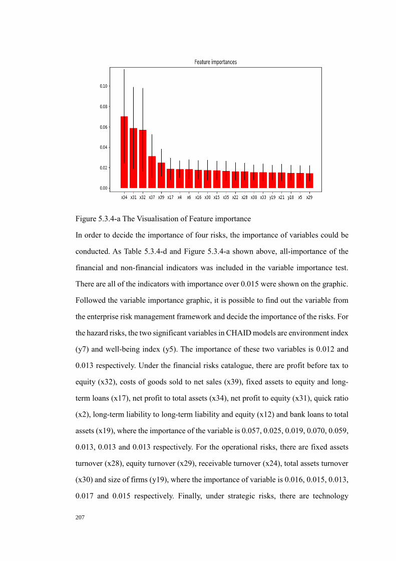
207
Figure 5.3.4-a The Visualisation of Feature importance
In order to decide the importance of four risks, the importance of variables could be
conducted. As Table 5.3.4-d and Figure 5.3.4-a shown above, all-importance of the
financial and non-financial indicators was included in the variable importance test.
There are all of the indicators with importance over 0.015 were shown on the graphic.
Followed the variable importance graphic, it is possible to find out the variable from
the enterprise risk management framework and decide the importance of the risks. For
the hazard risks, the two significant variables in CHAID models are environment index
(y7) and well-being index (y5). The importance of these two variables is 0.012 and
0.013 respectively. Under the financial risks catalogue, there are profit before tax to
equity (x32), costs of goods sold to net sales (x39), fixed assets to equity and long-
term loans (x17), net profit to total assets (x34), net profit to equity (x31), quick ratio
(x2), long-term liability to long-term liability and equity (x12) and bank loans to total
assets (x19), where the importance of the variable is 0.057, 0.025, 0.019, 0.070, 0.059,
0.013, 0.013 and 0.013 respectively. For the operational risks, there are fixed assets
turnover (x28), equity turnover (x29), receivable turnover (x24), total assets turnover
(x30) and size of firms (y19), where the importance of variable is 0.016, 0.015, 0.013,
0.017 and 0.015 respectively. Finally, under strategic risks, there are technology
208
innovation index (y8), tax rate (y16), cost of goods sold to net assets (x39), inventory
to current assets (x4), industry (y1) and inventory to total assets (x5), where the
importance of the variable is 0.013, 0.008, 0.025, 0.018, 0.009 and 0.015 respectively.
Therefore, it could be concluded that the financial risks are the most important risk
amongst total four risk types, where the most important indicators are net profit to total
assets (x34), profit before tax to equity (x32) and net profit to equity (x31). The most
important aspect of financial risks is profitability. The strategic risks and operational
risks are similarly important risks. The most important indicators for operation risks
are turnover ratios, while the most important indicators for strategic are inventory and
prime operating-related ratios. Accordingly, the most important element under
operational risks is business operations. Moreover, the most important element under
strategic risks is costumer wants and competition. For hazard risks, the two indicators
are similarly important, where could not be decided the importance. Therefore, if the
Chinese listed SMEs need to improve the performance, the financial risks are the most
critical risk they need to consider. The strategic risks and operational risks are the
secondary risks to be considered, while the Chinese listed SMEs can not neglect the
capital efficiency and prime operating activities.
In order to test the accuracy of the predicted models, the further test could be applied.
Since the result is a binary result, which means the performance could be only good
or poor in CHAID models, the receiver operation characteristic (ROC) curve could be
used to test the prediction accuracy. The ROC curve plots the true positive rate against
the false positive rate (SPSS, 14.2). For a good model, the curve will rise sharply near
the left axis and cut across near the top, which will draw a graph like a semicircle. For
an uninformative model, the curve will like a line with slope equal to 1.

209
Figure 5.3.4-b The Result of ROC curve of CHAID (ROA)

210
As the result of ROC shows, the highest AUC value is in the model A with CHAID,
which is 0.739. The AUC value is higher than the model B with CHAID (0.725) and
model C with CHAID (0.567). Fawcett (2006) introduced that the AUC is a portion of
the area of a unit square under the ROC curve, which means the AUC value should
always be between 0 and 1.0. For a unit square within a coordinate system, a randomly
guess could produce an area with the minimum square of 0.5 (Fawcett, 2006).
Therefore, it could be concluded that the model A with CHAID has the highest
accuracy in predicting firm performance and finding risk indicators. The model C with
CHAID could not explain the question well.
5.4 Logit Regression Results
5.4.1 Logit Regression
The Logit Regression is a standard statistical method, which has been developed from
the 1970s in early warnings of bank failure (Klistik, Kocisova and Misankova, 2015).
The LR could explain binary variables, which could be used to classify whether the
firm is failed or not. Spuchl’kova and Cug (2014) stated that the classic regression
could not be used under this circumstance if the value of the variable indicates the
status of “yes or no”. Thus, the Logit model was introduced to solve this kind of
problems. The aim of LR has expressed dependence of magnitude Y on the
independent variable X. The observed data are interleaved by a logistic curve instead
of a line, so that the regression is not linear. Meanwhile, the Logit Regression does not
require the data should follow a strictly normal distribution. The Logit transformation
is based on the “ratio of chances and hopes” (Klistik et al., 2015). Each LR function
could provide the AIC for the model, which could measure the effectiveness of the
regression. This research used LR to determine the KRIs and verify the value of non-

211
financial indicators.
The exhaustive method is used in LR regression for this research. In LR regression,
the AIC value will measure the accuracy of the model, so that the question was
transferred as finding out the minimum AIC value. The AIC value depends on the
independent indicators applied in the regression model, where the minimum AIC
means the most accurate result. As a result, the minimum AIC could be found by
attempting all the different combinations of indicators applied. The exhaustive method
will be applied in the selection of indicators included in the model. There are two
different ways of exhaustive, where the applied indicators could be from more to less
or less to more. The AIC values of each combination will be calculated, which will be
compared with each other to find out the minimum one. This step will be repeated
several times, where the repeated step could be considered as an iterative process.
5.4.2 Logit Regression with financial and non-financial
indicators
The dependent variable is selected as growth rate of ROA (ROA for short in the
following parts), which is a binary variable. The independent variables were selected
as financial indicators and non-financial indicators in this section.

212
Figure 5.4.2-a Result of LR with F and NF indicators
The Logit Regression could also be used to find the key risk indicators and explain the
risks. Figure 5.4.2-a above shows the model from the beginning, which contains forty-
two financial indicators and nineteen non-financial indicators. The AIC value is
1036.73 in the beginning model. In order to achieve a better result, it is necessary to
delete the insignificant variables in order to maximise the AIC value. After 42 times
of iteration steps, there are twelve financial indicators and five non-financial indicators
left in the Logit model.

213
Estimate Std.Error z value Pr(>|z|)
(Intercept) -6.90E-01 1.40E+00 -0.483 0.629 .
x2 9.60E-02 3.80E-02 2.487 0.013 *
x4 1.40E+00 6.00E-01 2.296 0.022 *
x8 2.90E+00 6.70E-01 4.29 0 ***
x10 -1.30E+07 7.40E+06 -1.751 0.08 .
x11 -1.30E+07 7.40E+06 -1.751 0.08 .
x17 8.20E-01 3.80E-01 2.174 0.03 *
x21 1.30E+07 7.40E+06 1.751 0.08 .
x31 7.30E+00 2.00E+00 3.638 0 ***
x34 -4.00E+01 5.00E+00 -8.109 0 ***
x38 1.70E-03 1.10E-03 1.481 0.139 .
x42 3.20E-04 1.80E-04 1.718 0.086 .
y2 3.20E-01 1.40E-01 2.299 0.021 *
y4 1.80E-02 8.00E-03 2.292 0.022 *
y10 -2.10E+00 1.10E+00 -1.899 0.058 .
y12 -2.00E-01 1.10E-01 -1.854 0.064 .
y14 -2.50E-01 1.30E-01 -1.945 0.052 .
Table 5.4.2-a Significant indicators of LR with F and NF indicators
The significance values of indicators were shown in Table 5.4.2-b. If the significance
value of variables was set as 0.05, there are x2, x4, x8, x17, x31, x34, y2 and y4 are
significant, which are quick ratio, inventory to current assets, equity to total assets,
fixed assets to equity and long-term loans, net profit to equity, net profit to assets,
number of employees and economic development index.

214
Predicted group 1 0
LOGIT Profit 1 66.88% 33.12% 70.71%
Loss 0 24.60% 75.40%
Table 5.4.2-b Prediction accuracy of F and NF indicators with LR
The prediction accuracy of Logit Regression is shown in Table 5.4.2-b. The data in
2012 was chosen as a training group, and the data in 2013 was chosen as a test group.
The overall prediction accuracy is 70.71%.
5.4.3 Logit Regression with financial indicators
The dependent variable is selected as growth rate of ROA. The independent variables
were selected as financial indicators only in this section.

215
Figure 5.4.3-a Result of LR with F indicators
The results of Logit Regression with financial indicators only were shown in Figure
5.4.3-a. After 26 iterations, there are only 12 variables left. The AIC value was
improved from 1026.97 to 984.1. The iteration steps were stopped since the AIC value
cannot be reduced. There are x2, x5, x10, x11, x13, x21, x22, x23, x31, x34, x38 and
x42 were left in the formula.
Estimate Std.Error z value Pr(>|z|)
(Intercept) 1.58E+00 5.49E-01 2.867 0.004 **
x2 1.00E-01 3.91E-02 2.568 0.01 *
x5 2.21E+00 8.91E-01 2.483 0.013 *
x10 -1.22E+07 7.26E+06 -1.679 0.093 .
x11 -1.22E+07 7.26E+06 -1.679 0.093 .
x13 -1.30E+00 8.44E-01 -1.545 0.122
x21 1.22E+07 7.26E+06 1.679 0.093 .
x22 -1.83E+00 6.41E-01 -2.852 0.004 **
x23 2.59E+00 7.64E-01 3.392 0.001 ***
x31 6.15E+00 1.98E+00 3.115 0.002 **
x34 -3.79E+01 4.82E+00 -7.878 0 ***
x38 1.40E-03 1.12E-03 1.253 0.21
x42 2.81E-04 2.06E-04 1.362 0.173
Table 5.4.3-a Significant indicators of LR with F indicators
The Table 5.4.3-a shows the z-values of indicators. If the significance level is 0.05, the
x2, x5, x22, x23, x31 and x34 are significant, which are quick ratio, inventory to total
assets, current assets to total assets, tangible fixed assets to total assets, net profit to
equity and net profit to assets.

216
Groups 1 0
LOGIT Profit 1 64.94% 35.06% 68.98%
Loss 0 26.98% 73.02%
Table 5.4.3-b The Prediction accuracy of F indicators with LR
Table 5.4.3-b above shows the model accuracy of Logit Regression with financial
indicators, where the overall accuracy is 68.98%. The training set and test set selection
is the same as the Logit Regression with financial indicators and non-financial
indicators model.
5.4.4 Logit Regression with non-financial indicators
The dependent variable is selected as the growth rate of ROA. The independent
variables were selected as non-financial indicators only in this section.
Figure 5.4.4-a Result of LR with NF indicators
Figure 5.4.4-a above showed the result of Logit Regression with non-financial

217
indicators only. In the beginning, there are nineteen non-financial indicators were
included in the model. After eight times iterations, there are only eight variables left
in the model. The AIC was improved from 1162.72 to 1151.89. The eight variables are
y3, y4, y5, y6, y7, y8, y10, y14, y17 and y19.
Estimate Std.Error z value Pr(>|z|)
(Intercept) 3.68977 3.83546 0.962 0.33604
y3 -
1.00576 0.46441 -2.166 0.03034 *
y4 0.21761 0.10262 2.121 0.03396 *
y5 0.27097 0.1258 2.154 0.03124 *
y6 0.2171 0.12652 1.716 0.08617 .
y7 0.20449 0.09145 2.236 0.02534 *
y8 0.12651 0.0576 2.196 0.02807 *
y10 -
2.31224 1.07007 -2.161 0.03071 *
y14 -
0.27044 0.10283 -2.63 0.00854 **
y17 0.31125 0.15378 2.024 0.04297 *
y19 -
0.19107 0.09527 -2.005 0.04492 *
Table 5.4.4-a Significant indicators of LR with NF indicators
Table 5.4.4-a shows the z-values of indicators. If the significance level was set as 0.05,
the variables y3, y4, y5, y7, y8, y10, y14, y17 and y19, which are develop and life
index, economic development index, well-being index, environment index,
technology innovation index, audit opinions, number of employees, listed duration and
size of firms.

218
Group 1 0
LOGIT Profit 1 50.92% 49.08% 53.67%
Loss 0 43.59% 56.41%
Table 5.4.4-b The Prediction accuracy of NF indicators with LR
Table 5.4.4-b shows the overall accuracy of the Logit Regression model with non-
financial indicators is 53.67%. The training set and test set selection is the same as the
Logit Regression with financial indicators and non-financial indicators model.
5.4.5 Summary
The Logit Regression method also selected forty-two financial variables and nineteen
non-financial variables. The dependent variable was selected as the growth in ROA
rather than Z-score since the Logit Regression requires a binary dependent variable.
The Logit Regression is also used for the selection of KRIs among risk indicators. To
select the KRIs amongst risk indicators, it followed a combination of financial and
non-financial indicators, only financial indicators and only non-financial indicators.
The usage of different groups could be helpful to find the KRIs and the value of non-
financial indicators. The measurement of performance is AIC value, which could
produce a satisfactory solution to the target problems based on the number of factors
(Akaike, 1987). Akaike (1987) stated that the minimum AIC represents the best fit. In
this research, the process to select the variables with the LR regression could be
described as follow: include all the groups of indicators first and get the result; exclude
one of the indicators and get the result; compare the AIC from two groups and choose
the minimum AIC; repeat the process until the AIC reached the minimum. It is also
important to check the significant value of indicators, where the insignificant variable
should be excluded from KRIs. After using three different groups of indicators, it is
possible to conclude the KRIs from indicators.

219
Groups Code Indicators
F and NF x2 quick ratio
x4 inventory to current assets
x8 equity to total assets
x17 fixed assets to equity and long-term loans
x31 net profit to equity
x34 net profit to assets
y2 number of employees
y4 economic development index
F x2 quick ratio
x5 inventory to total assets
x22 current assets to total assets
x23 tangible fixed assets to total assets
x31 net profit to equity
x34 net profit to assets
N y3 develop and life index
y4 economic development index
y5 wellbeing index
y7 environment index
y8 technology innovation index
y10 audit opinions
y14 number of employees
y17 listed duration
y19 size of firms

220
Figure 5.4.5-a Significant indicators in all LR models and feature importance
Figure 5.4.5-a shows the significant variables and feature importance. Although the
significance of indicators to firm performance could be detected, it is not possible to
decide the threshold values and the order of importance based on the LR method only.
As a result, it is necessary to use extra methods to decide the KRIs, where the variable
importance could be a choice. As the graph above shows, the 21 indicators with the
highest importance have been detected. It could be concluded that x4, x5, x17, x31,
x34 and y19 matched the result of variable importance. Therefore, it could say that the
x4, x5, x17, x31, x34 and y19 are KRIs from the LR method, where the threshold
values and roadmaps could not be detected by using LR method.
The research also considered applying the CHAID and LR method together in order
to find threshold values and roadmaps. Since the CHAID method runs a Chi-square
test on each independent variable to dependent variable and every node, it is clear that
the CHAID potentially consider all the variables to build the decision tree. If the Logit
Regression was implied before building CHAID, it is possible that the hierarchy nodes
and branches will be reduced. There is a problem called overfitting. Hawkins (2004)
stated that models and procedures should contain all necessary but nothing more. For

221
example, if a regression model with two indicators can explain the dependent variable,
there should no more than these two indicators be included. The overfitting problem
is that the usages of models or procedures violate such parsimony, which includes
more terms than necessary or uses more complicated approaches than necessary.
Therefore, since the CHAID and Logit Regression may overlap on the variable
classification or test, it is better to use only one of these methods separately.
5.5 Genetic Algorithm Results
5.5.1 Genetic Algorithm in variable selection
Genetic algorithms (GA) are population-based evolutionary searching methods. These
algorithms have used probability-based search methods, which gained ideas drawn
from natural genetic and evolutionary principles (Chamber, 1995). Genetic algorithms
are particularly suitable for solving scheduling and machine layout problems. The
genetic algorithms differ from other non-linear optimization techniques. In a genetic
algorithm, a population of strings, which encode a potential solution to the problem,
is evolved toward a better solution (Chamber, 1995). A population of candidate
solutions, whose individuals are characterised by possessing a chromosome, is
maintained, and after a generation is accomplished, the population evolves until
converges at levels regarded as optimal. The evolution (initialisation stage) usually
starts from a population of randomly generated individuals and happens in generations.
Each chromosome is evaluated utilising a user-defined fitness function. For real-world
applications of GAs, choosing the fitness function is the most critical step. In each
generation, the fitness of every individual in the population is evaluated, multiple
individuals are stochastically selected from the current population (based on their
fitness), and modified (recombined and possibly randomly mutated) to form a new
population. The new population is then used in the next iteration of the algorithm. The

222
algorithm terminates when a maximum number of generations has been produced, or
a satisfactory fitness level has been reached for the population.
In this study, the fitness value is the Cross Validation, which indicates the accuracy of
the predicting result. For example, if 10-fold cross-validation is selected, the entire
genetic algorithm is conducted ten separate times. For the first fold, nine-tenths of the
data are used as comparing groups, while the remaining tenth is used to estimate the
result. Moreover, this process will be repeated ten times, while the accuracy will be
compared after that. This function determines the optimal number of generations for
the GA. In order to get the best results, the indicators were regrouped as many as
possible. If the indicators produced lower accuracy predicted results, the indicators
would be removed from the training set. Since the iteration process needs
exceptionally high computing power, the maximum iteration times were set as three
times.
5.5.2 Genetic Algorithm with financial and non-financial
indicators
In this section, the individuals were selected from forty-two financial indicators and
nineteen non-financial indicators. The method aims to select the most important
indicators from all input neurons.
Iterations Variables Accuracy Kappa Accuracy SD Kappa SD
1 1 0.6269 0.2476 0.09421 0.1906
2 2 0.7265 0.448 0.07791 0.1578
3 3 0.7449 0.486 0.06549 0.1307

223
4 4 0.7495 0.4943 0.07077 0.1436
5 5 0.7517 0.5008 0.06889 0.1374
6 6 0.7494 0.496 0.1024 0.2066
7 7 0.7676 0.5311 0.08542 0.1733
8 8 0.7607 0.5179 0.07919 0.1606
Table 5.5.2 Result of GA with Financial and Non-Financial Indicators (1)
There are forty-two financial indicators, and nineteen non-financial indicators were
used as individuals. Table 5.5.2 shows the iterations, number of variables and accuracy
of the method. For the financial indicators and non-financial indicators group, the
accuracy of the predicted result reached the maximum at seven variables left.
Figure 5.5.2-a Result of GA with Financial and Non-Financial Indicators (2)
As Figure 5.5.2-a shows, the maximum accuracy is 0.7676. To find out the most
important indicators, it is also necessary to apply the feature importance method.

224
Figure 5.5.2-b The Features Importance of GA with F and NF Indicators
As Figure 5.5.2-b above shown, the most important indicators are x31, x32, x34, x37,
x33, x3 and x12, which are net profit to equity, profit before tax to equity, net profit to
assets, gross profit to net sales, EBIT to EBT and finance expense, absolute liquidity,
and long-term liability to long-term liability and equity. The seven indicators are all
financial indicators. It means that the firm performance prediction with the GA method
mostly depended on the financial indicators than non-financial indicators.
5.5.3 Genetic Algorithm with financial indicators
In this section, the individuals are selected as financial indicators only. There are total
forty-two financial indicators were used in this part.
Iterations Variables Accuracy Kappa Accuracy SD Kappa SD
1 1 0.646844 0.2900703 0.05338264 0.10295596
2 2 0.7378201 0.4732482 0.04489754 0.08560919
3 3 0.7630796 0.5237937 0.04315571 0.08598116
4 4 0.7586375 0.5150284 0.04773482 0.09330309

225
5 5 0.7472187 0.4914868 0.04845589 0.09483429
6 6 0.7518147 0.5001206 0.06731957 0.13304206
7 7 0.7496453 0.4967097 0.05543584 0.10863941
8 8 0.7519204 0.5001481 0.05826773 0.11675416
Table 5.5.3 The Result of GA with Financial Indicators (1)
Table 5.5.3 shows the iterations, number of variables and accuracy in this method. The
method reached the highest accuracy when the number of variables equals to 3. At this
point, the predicted accuracy is 0.7630.
Figure 5.5.3-a The Result of GA with F indicators (2)
As Figure 5.5.3-a shown, the accuracy is increased significantly as the number of
variables increased until there are three variables were included. After this point, the
accuracy fluctuated until the number of variables reached eight. Then, the accuracy
was increasing slowly as the number of variables increases. The accuracy of prediction
could not exceed 0.76 as the number of indicators increased until the number of
variables reached the maximum.

226
Figure 5.5.3-b Features Importance of GA with F Indicators
In order to detect the most important indicators, it is necessary to use feature
importance method to measure the importance of indicators. As Figure 5.5.3-b shows,
the most important indicators are x31, x32 and x34, which are net profit to equity,
profit before tax to equity and net profit to assets respectively.
5.5.4 Genetic Algorithm with non-financial indicators
In this section, the individuals are selected as non-financial indicators only. There are
total nineteen non-financial indicators were used in this part.
Iterations Variables Accuracy Kappa Accuracy SD Kappa SD
1 1 0.5239464 -0.0102644 0.0211053 0.0270737
2 2 0.5262192 -0.0079348 0.0121068 0.0135439
3 3 0.5105626 -0.0172180 0.0542413 0.1042585
4 4 0.4984202 -0.0206483 0.0768341 0.1604554
5 5 0.4988384 -0.0123038 0.0545900 0.1154158
6 6 0.4851492 -0.0421573 0.0517080 0.1079851
7 7 0.5078788 0.0034385 0.0500580 0.1024859
15.03821378 15.00426021
12.30907294
0
2
4
6
8
10
12
14
16
x31 x32 x34
Feature Importance

227
8 8 0.4850987 -0.0407024 0.0683793 0.1327973
Table 5.5.4 The Result of BPNN with NF Indicators (1)
Table 5.5.4 shows the iterations, number of variables and accuracy in this method. The
highest accuracy has been reached, when the number of variables equals to two. At the
moment, the accuracy is 0.526.
Figure 5.5.4-a The Result of GA with NF indicators (2)
As Figure 5.5.4-a shows, the accuracy of GA with non-financial indicators is
fluctuating dramatically. After the highest accuracy has been reached at number of
variable equals 2, the accuracy dropped significantly till number of variable equals 6.
Afterwards, the accuracy of prediction could not exceed 0.52 as the number of
indicators increased.

228
Figure 5.5.4-b Features Importance of GA with NF Indicators
Figure 5.5.4-b shows the result of feature importance. In order to detect the most
important indicators, it is necessary to use feature importance method to measure the
importance of indicators. As Figure 5.5.4-b shown, the most important indicators are
y10 and y9, which are audit opinions and education background of employees
respectively.
5.5.5 Summary
The GA methods have applied three different groups of indicators, which are financial
and non-financial indicators, financial indicators only and non-financial indicators
only. The fitness value of GA is selected as the accuracy of cross validation, where the
value is going to measure internal performance. In other word, the accuracy of cross-
validation has been applied in selecting the number of indicators. Specifically, for the
GA methods, including non-financial indicators could slightly increase the accuracy
of cross validation from 0.763 (financial indicators only) to 0.767 (financial indicators
and non-financial indicators. It is clear that the non-financial indicator groups have the
worst performance in the GA method, where the accuracy is only 0.526. It is clear that
the GA method determines the firm performance mostly depending on the financial
4.385605748
2.295658305
0
0.5
1
1.5
2
2.5
3
3.5
4
4.5
5
y10 y9
Feature Importance

229
indicators since the accuracy of non-financial indicators group is only 0.526. However,
it has been confirmed that including the non-financial indicators could increase the
accuracy of the GA method. After three iterations, the financial and non-financial
indicators group has 4 more indicators than financial indicator group only, which
means including non-financial indicators could provide more comprehensive
information.
GA Real group Predicted group
Firms correctly (incorrectly)
classified
1 0
Financial and
non-financial
indicators
Profit 1 70.59% 29.41%
74.87%
Loss 0 20.85% 79.15%
Financial
indicators
Profit 1 73.53% 26.47%
75.91%
Loss 0 21.70% 78.30%
Non-financial
indicators
Profit 1 0.00% 100.00%
47.38%
Loss 0 1.70% 98.30%
Figure 5.5.5-a The Prediction accuracy of all GA models
Figure 5.5.5-a shows the prediction accuracy of GA models with three different groups
of indicators. There is only a slight difference between the accuracy of GA with
financial and non-financial indicators model and GA with financial indicators model.
Comparing two models, the GA with financial and non-financial indicators model
predicted poor performance firms better than the GA with financial indicator model.
The prediction accuracy of both models is acceptable, where the accuracy is around
75%.
On the contrary, the accuracy of GA with non-financial is only 47.38%, which means
the model cannot be used to predict the firm performance. However, the prediction

230
accuracy of poor performance firms with the model is 98.3%, while the prediction
accuracy of good performance firms with the model is 0%. The result indicates that
the non-financial indicators groups cannot be used to predict the firm performance.
The predicted group could be classified all of the samples in one catalogue, which may
result in the fifty-fifty result. This kind of result is more like the statistical experiment
‘coin tossing’, which result randomly 50% for each catalogue. For instance, the model
classified all of the samples in poor performance, which will result in the 100% for
poor performance firms prediction, but 0% for good performance firms. Therefore, it
could be concluded that the non-financial indicators cannot be independently used to
predict firm performance. On the other hand, the financial and non-financial indicator
group and financial indicator group models could be used to predict firm performance.
Since both models have more than 74% accuracy for two predicted groups, it means
that the result is not like non-financial indicators model. The accuracy was slightly
dropped by including non-financial indicators to the model, where the highest
accuracy among GA models is the one with financial indicators group.
Groups Overall Var
F and NF 1 15.12184885 x31 net profit to equity
2 12.94503794 x32 profit before tax to equity
3 12.07511835 x34 net profit to asset
4 8.728316218 x37 gross profit /net sales
5 4.852187639 x33 EBIT/EBT and Finance expense
6 3.93329857 x3 absolute liquidity
7 3.574172304 x12 long-term liability to long-term liability and equity
F 1 15.03821378 x31 net profit to equity
2 15.00426021 x32 profit before tax to equity
3 12.30907294 x34 net profit to asset
NF 1 4.385605748 y10 audit opinions

231
2 2.295658305 y9 employees education
Figure 5.5.5-b Significant indicators of GA models
Figure 5.5.5-b indicated the different significant indicators in three different models
by GA methods. Although the accuracy of GA with financial indicators is slightly
higher than GA with financial and non-financial indicators, more variables are
significant in the latter one. Compared the two different models, the financial and non-
financial indicators considered the cost, tax, liquidity and liability than financial
indicators model, which may provide more comprehensive information regarding the
enterprise risk management framework. It could be concluded that the non-financial
indicators will indirectly improve the predictive results in the risk management
process, which included the features under operational risks and strategic risks. Figure
5.5.5-b also shows the GA model with financial indicators model only included three
risks, which are the features of financial risks only. As a result, the non-financial
indicators could provide more information to decision makers in considering all the
risks.
5.6 Neural Network Results
5.6.1 BPNN
The (artificial) neural network (NN) is made up of a large number of neurons and
connections between them (Back, Laitinen and Sere, 1996). The neurons in the
networks are arranged in the layers, which included input layers, hidden layers and
output layers. Each layer is fully interconnected to the preceding layer and the
following layer (SPSS, 2011). It is necessary to determine the weights of neurons,
which are used to connect each layer. Based on the weights, the importance of the
neurons could be described. Meanwhile, the weights could be adjusted iteratively in
order to generate better prediction results. The network starts to mimic the biological

232
neural network, which one neuron passes information to another. In the neural network,
the input layers contained input neurons, which determined the neurons in output
layers via hidden layers. Since the weights are learned using iteration, the network
could get a desirable input to output by a learning mechanism (Back et al., 1998).
There are two different types of learning mechanism of learning, which are supervised
learning and unsupervised learning. The supervised learning is used to get the answers
to a specific question, which is firm performance in this study. Unsupervised learning
is to get answers to unknown questions. The target problems are defined by KPIs and
the target data set is used to select KRIs, all of the output and input are certain, so that
unsupervised learning may not be suitable for this study.
The backpropagation artificial neural network (BPNN) means the model is not a
simple feed-forward neural network, where it uses backpropagation to iteratively
adjust the weights of neurons to get the minimum error output (IBM, 2011; Back et
al., 1996). The information flow goes through the network from the input layer to the
output layer, then get a prediction result. The prediction result is compared with the
recorded value of the output layer to calculate the error, while the difference between
the predicted and actual output is propagated backward through the network (IBM,
2011). At the start of training, the weights of neurons are randomly valued between -
0.5 and 0.5. During cycles from the input layer to the output layer, the weights of the
neurons will be continuously adjusted based on the errors of prediction results. After
several iterations, the error could be minimized, and the prediction results will be close
to the actual result. The errors were measured by the sum of squared errors of
prediction (SSE). Therefore, the final result shows the minimised error between the
actual value and prediction result by iteratively adjusting the weights of input neurons.

233
5.6.2 BPNN with financial and non-financial indicators
In this section, the input neurons were selected as financial and non-financial
indicators. There are forty-two financial indicators, and nineteen non-financial
indicators were used in this part. The detailed results were listed in Appendix 2, Table
5.6.2-a and Table 5.6.2-b.
Figure 5.6.2-a The Result of BPNN with F and NF indicators
Figure 5.6.2-a shows the SSE of BPNN with financial and non-financial indicators.
The weighted SSE, which shows as a black line, is converged with less than 40 after
200 times iterations. In the beginning, the SSE decreased significantly from 150 to 75.
After 50 times iterations, the SSE decreased slowly from 75 to 35. The difference
between the highest SSE to the lowest is about 120. The red line shows the SSE in the
test set, which is around 110. The converging speed of the test set line is respectively
lower than the training set. During the 50th iteration and 150th iteration, there are
continually fluctuating between 110 and 130. The SSE of the test set finally converged
to around 130. The table 5.6.2-a shows all the neurons applied in the BPNN method.
The performance is measured as a binary variable, where value 1 represents good, and
0 represent poor. As the table 5.6.2-a shown, it is clear that the value of output neurons

234
converged to 1 and 0. In order to verify the training result, the rules should be applied
to the test set.

235
Model
Real group
membership
Predicted group
Firms correctly(incorrectly)
classified
1 0
BP Profit 1 68.97% 31.03%
67.59%
Loss 0 33.78% 66.22%
Figure 5.6.2-b Prediction accuracy of BPNN with F and NF indicators
As Figure 5.6.2-b shows, the overall prediction accuracy of BPNN with financial and
non-financial indicators is 67.59%. The prediction accuracy of good performance
firms is 68.97%, while the prediction accuracy of poor performance is 66.22%. The
prediction accuracy of good performance firms is a little bit higher than the other one.
Figure 5.6.2-c The ROC curve of BPNN with F and NF indicators
Figure 5.6.2-c shows the result of the ROC test. In order to test the accuracy of the
predicted models, the ROC test could be applied. The receiver operation characteristic
(ROC) curve could be used to test the accuracy since the results are binary. The area
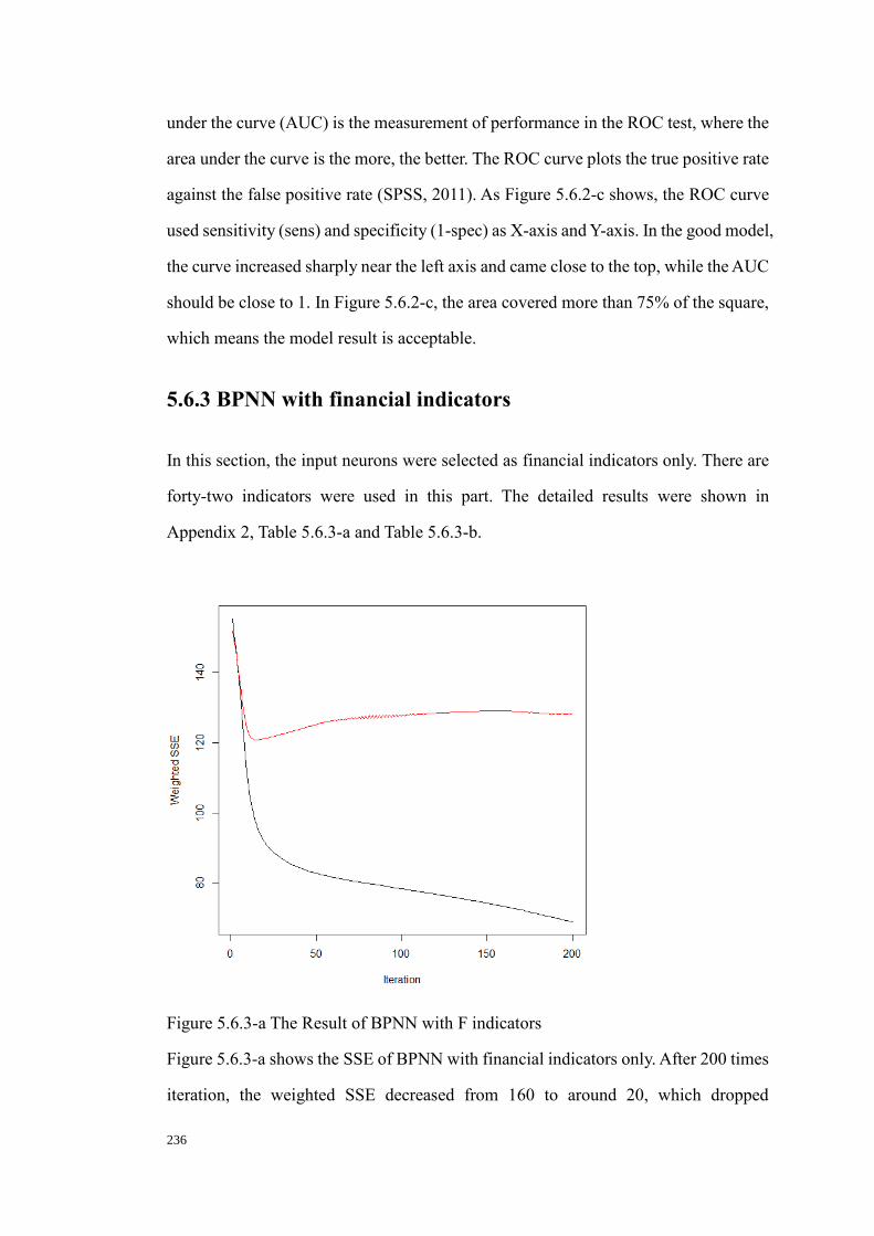
236
under the curve (AUC) is the measurement of performance in the ROC test, where the
area under the curve is the more, the better. The ROC curve plots the true positive rate
against the false positive rate (SPSS, 2011). As Figure 5.6.2-c shows, the ROC curve
used sensitivity (sens) and specificity (1-spec) as X-axis and Y-axis. In the good model,
the curve increased sharply near the left axis and came close to the top, while the AUC
should be close to 1. In Figure 5.6.2-c, the area covered more than 75% of the square,
which means the model result is acceptable.
5.6.3 BPNN with financial indicators
In this section, the input neurons were selected as financial indicators only. There are
forty-two indicators were used in this part. The detailed results were shown in
Appendix 2, Table 5.6.3-a and Table 5.6.3-b.
Figure 5.6.3-a The Result of BPNN with F indicators
Figure 5.6.3-a shows the SSE of BPNN with financial indicators only. After 200 times
iteration, the weighted SSE decreased from 160 to around 20, which dropped

237
significantly from 160 to 90 at around 40th iteration. After that, the weighted SSE
decreased slowly to 200th iteration. The difference between the highest SSE to the
lowest SSE is 140. The SSE of training set decreased significantly from 150 to 120 in
the first 20 iterations. After that, it smoothly increased about 5, while finally converged
to 125. Table 5.6.3-a shows the values of each neuron, while the important ones are
the value of output layers. Table 5.6.3-b shows the weighted value of hidden neurons
and output neurons. The most important thing is that the converging values of the
model are not close to 0 and 1, which means the result may not be able to classify the
poor performance and good performance firms.
Model
Real group
membership
Predicted group
Firms correctly(incorrectly)
classified
1 0
BP Profit 1 68.97% 31.03%
68.94%
Loss 0 31.08% 68.92%
Figure 5.6.3-b The Prediction accuracy of BPNN with F indicators
The prediction result is shown in Figure 5.6.3-b. The overall prediction accuracy for
BPNN with financial indicators is 68.94%. The prediction accuracy for good
performance firms is 68.97%, while the prediction accuracy for poor performance
result is 68.92%. There is not a significant difference between the prediction accuracy
for good or poor performance firms.

238
Figure 5.6.3-c ROC curve of BPNN with F indicators
Figure 5.6.3-c shows the result of the ROC test. As mentioned before, the AUC should
be close to 1, which indicates the prediction accuracy is good. As the figure shows, the
AUC is greater than 0.5, while the total AUC is around 75% of the full area. Therefore,
it indicates that the result could explain well.
5.6.4 BPNN with non-financial indicators
In this section, the input neurons were selected as non-financial indicators. There are
nineteen non-financial indicators were used in this part. The detailed results were listed
in Appendix 2, Table 5.6.4-a and Table 5.6.4-b.

239
Figure 5.6.4-a The Result of BPNN with NF indicators
Figure 5.6.4-a shows the result of BPNN with non-financial indicators only. The
weighted SSE smoothly dropped from around 160 to 110 after 200 times iteration.
Although the process is smooth, the absolute difference between the highest SSE to
the lowest is about 50. The SSE of training set cannot converge to a stable value. It
shows the SSE of training set increased over 150, while the converged value does not
exist during the 200 iterations. Table 5.6.4-a shows the value of each neuron in the
network. The value of the output layer did not converge to 0 and 1, where is around
40:60. Table 5.6.4-b shows the weighted value of each neuron in the hidden layer.
Model
Real group
membership
Predicted group
Firms correctly(incorrectly)
classified
1 0
BP Profit 1 27.59% 72.41%
41.50%
Loss 0 44.59% 55.41%
Figure 5.6.4-b The Prediction accuracy of BPNN with NF indicators
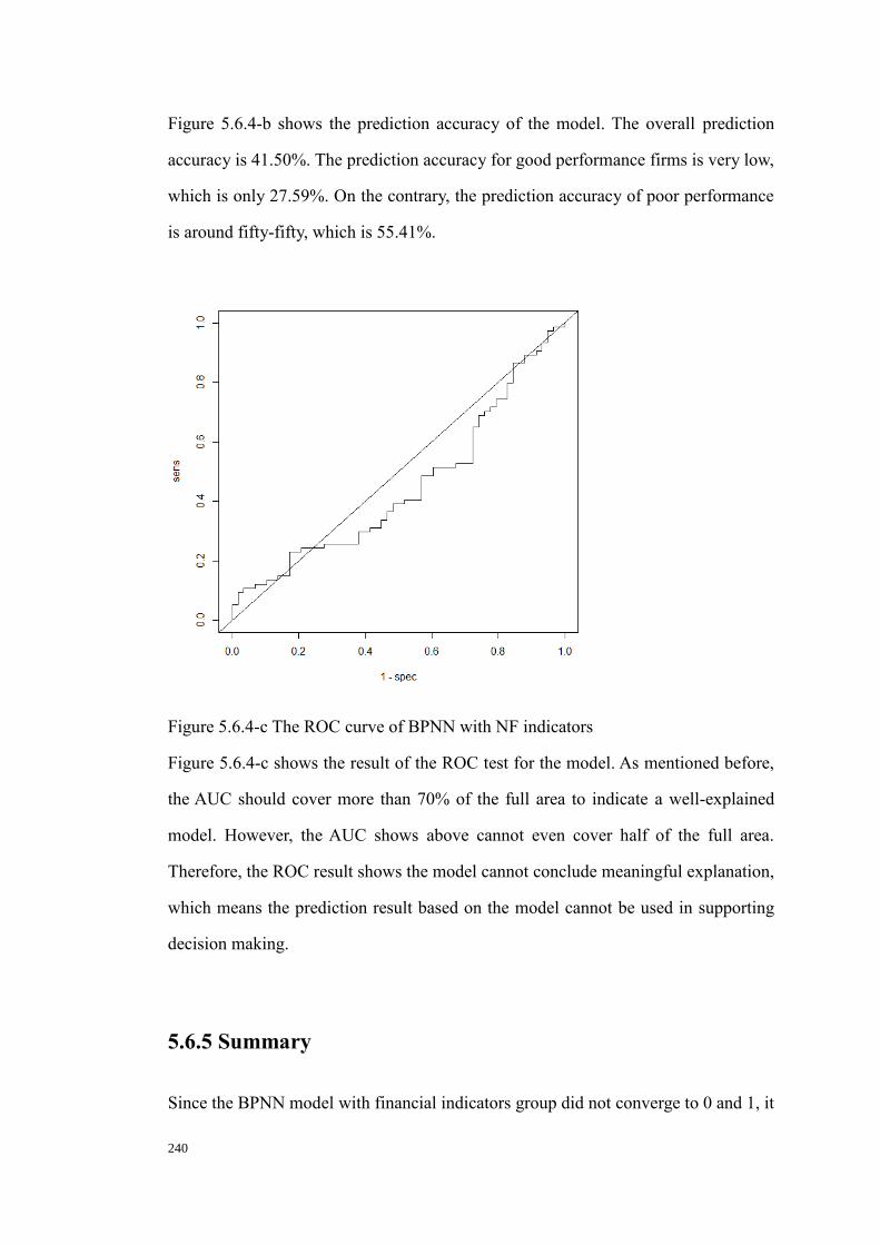
240
Figure 5.6.4-b shows the prediction accuracy of the model. The overall prediction
accuracy is 41.50%. The prediction accuracy for good performance firms is very low,
which is only 27.59%. On the contrary, the prediction accuracy of poor performance
is around fifty-fifty, which is 55.41%.
Figure 5.6.4-c The ROC curve of BPNN with NF indicators
Figure 5.6.4-c shows the result of the ROC test for the model. As mentioned before,
the AUC should cover more than 70% of the full area to indicate a well-explained
model. However, the AUC shows above cannot even cover half of the full area.
Therefore, the ROC result shows the model cannot conclude meaningful explanation,
which means the prediction result based on the model cannot be used in supporting
decision making.
5.6.5 Summary
Since the BPNN model with financial indicators group did not converge to 0 and 1, it

241
is possible to optimise the result by increasing the iteration times and the number of
hidden neurons. The detailed results were shown in Appendix 2, Table 5.6.5-a.
Figure 5.6.5-a Result of BPNN with F indicators (1000 times iterations)
Figure 5.6.5-a shows the weighted SSE in 1000th iterations, where the black line shows
the SSE of the training set and the red line shows the SSE of the test set. The table
5.6.5-a shows the values of output neurons, which are 0.998 and 0.00. The values of
output neurons are close to 0 and 1. However, the result still could not be used to
predict firm performance. The SSE of the test set in Figure 5.6.5-a did not coverage to
a constant value, on the contrary, the SSE of training set continually decreased as
iteration times increased. Although the SSE of the training set is quite low as iteration
increased, the increasing SSE of test set indicates that the rules cannot be applied with
other samples than the training set. More specifically, increased iterations led to the
problem of overfitting, which means the patterns or rules found by the training set
could only explain itself only. Therefore, the result in section 5.6.3 was selected as a
final result, since increasing iteration times cannot improve the model.

242
Indicators Real group membership Predicted group Firms correctly(incorrectly) classified
Financial and non-financial
1 0
Profit 1 68.97% 31.03%
67.59%
Loss 0 33.78% 66.22%
Real group membership Predicted group Firms correctly(incorrectly) classified
Financial
1 0
Profit 1 68.97% 31.03%
68.94%
Loss 0 31.08% 68.92%
Real group membership Predicted group Firms correctly(incorrectly) classified
Non-financial
1 0
Profit 1 27.59% 72.41%
41.50%
Loss 0 44.59% 55.41%
Figure 5.6.5-b The Prediction accuracy of three BPNN models
Figure 5.6.5-b shows the summary of the prediction accuracy of BPNN models with
three different indicator groups. The most accurate one is the BPNN with financial
indicators model, which is 68.94%. The BPNN with financial and non-financial
indicators model is the second accurate one, which the prediction accuracy is 67.59%.
There is not a significant difference between these two models. The prediction of good
performance firms is same for two models, while there is a slight difference (2.7%)
with the prediction of poor performance firms. However, the prediction accuracy of
BPNN with non-financial indicators model is inferior, which is only 41.5%.
Specifically, the prediction of good performance firms in BPNN with non-financial
indicators is the worst one, which is only 27.59%. Therefore, it could be concluded
that the most accurate model is BPNN with financial indicators. The prediction

243
accuracy will slightly decrease when the financial indicators and non-financial
indicators are used simultaneously in the model. According to the result, the non-
financial indicators cannot be solely used as input neurons to build the BPNN model.
SSE
Converging speed
(Training set)
Converging speed (Test
set)
Absolute
difference
AUC
Financial and non-
financial
quick at beginning
Quick at the beginning,
fluctuating
120 0.75
Financial quick at beginning
Quick at the beginning,
Smooth
140 0.75
Non-financial slow Does not converge 40
less than
0.5
Figure 5.6.5-c Description of three BPNN models
Figure 5.6.5-c shows the result of weighted SSE calculated by BPNN with three
different indicator groups. The result of the financial and non-financial indicators
group is very similar to the financial indicator groups. The Converging speeds of SSE
in training set in both groups are quick at the beginning, while the shape of the curve
is also similar. The converging speeds of SSE in the test set are different. As shown in
Figure 5.6.5-b, the converging speed of SSE for the test set in financial and non-
financial indicators group is quick at the beginning, but the whole process comes with
fluctuations. The converging speed of SSE for the test set in financial indicators group
is quick at the beginning but smoother than the previous group.
On the other hand, the SSE for the test set in non-financial indicators group does not
converge to a specific value after 200 iterations, which means the methods cannot be
used to predict with non-financial indicators group. There is only a slight difference in
the Absolute difference of weighted SSE, where the value of the Absolute difference
in financial indicators group is 20 higher. The AUC of both groups is the same, which

244
is shown in Figure 5.6.2-c and Figure 5.6.3-c. On the contrary, the Converging speed
of weighted SSE in non-financial indicator group is slow, where the value of the
Absolute difference is only 40. Most importantly, the AUC is less than 0.5, which
means it cannot explain the result well. Therefore, for BPNN models, the best one is
BPNN with financial indicators and including non-financial indicators simultaneously
with financial indicators cannot increase the prediction accuracy.
5.7 Summary
This chapter has shown the analytical procedures and the results of the analysis. There
are 849 listed Chinese SMEs in Shenzhen Stock Exchange has been selected. The data
was collected by Web Clawer. The main steps of applied data mining methods were
using SPSS 20.0 and R programming.
Firstly, the data was collected as discussed in previous chapters, which includes
financial information and non-financial information. Then, all the information was
transferred into indicators. After that, the financial ratios were calculated, and the non-
financial indicators were generated. The results of K-means clustering supported that
there are two different groups of firms, which means the classification should not
strictly follow ST/Non-ST standards in Chinese stock market.
Then, the CHAID, LR, GAs and BPNN were applied as data mining methods.
Followed the ERM framework, the dependent variables are KPIs and independent
variables are candidates of KRIs. To investigate the value of non-financial indicators
in DM-RM model, the KRIs were selected from three indicator groups, which are
financial and non-financial indicators groups, financial indicators group and non-
financial groups. In the CHAID method, the dependent variables are selected as Z-
score (Altman et al., 2010) and growth of ROA. In the rest three methods, the

245
dependent variables are selected as the growth of ROA. In order to provide additional
tests to verify the meaningfulness and robustness of the results, the variable
importance and RUC test have also been applied. At the end of each subsection, the
results of the data mining methods were summarised. Also, the rules and patterns
found by the data mining methods have also been initially discussed. The subsequent
chapter will discuss the results generated from this part and provide links between
results, hypothesis and findings.

246
6. Discussion
6.1 Introduction
This Chapter is going to discuss the main findings of the data mining methods. The
data mining process examined the usefulness and meaningfulness of KPIs and KRIs
in the DM-RM model. In order to test the relationship between the KPIs and KRIs,
four different data mining methods were applied in the empirical examination. The
data mining methods examined the selection of KPIs, selection of KRIs, the value of
non-financial indicators and the combination of data mining process and risk
management process.
The study has developed a research model that linked data mining process and risk
management process together. In order to improve the risk management process, the
data mining process was fitted into all steps in the risk management process. The two
processes were linked by using KPIs and KRIs. Meanwhile, the usage of EWS and BI
helped the DM-RM model focused on a specific purpose in this study. These
components improved the DM-RM model in risk treatment, data collection, and data
clean up. The usage of DM-RM model successfully captured the rules and patterns in
listed Chinese SMEs, which indicated the model is suitable for analysis of specific
targets. Furthermore, the results of this research were compared with other scholars’
work to verify the effectiveness of accuracy.
The purpose of this chapter is to provide a thorough discussion of all results obtained
from empirical examinations in the previous chapter. In doing so, this chapter was
divided into seven sections, including this introductory part. The following section 6.2
and 6.3 discusses the selection of KPI and KRIs. Next, the rules and patterns found by
the DM-RM model were detailed explained. After that, the hypotheses of this research

247
have been verified. Then, the results of this study have been compared to other studies
in order to verify the effectiveness. At last, a summary of this chapter is provided.
6.2 Selection of KPI
Coleman (2009) claimed that key risk indicators (KRIs) provided the information
about companies’ risk positions to alert the companies about the changes, which can
be used by management to show the risk level of activities and projects. Meanwhile,
according to Verbano and Venturini (2011), the purpose of ERM is to maximise the
firms’ value. It is also important for firms to present their profitability to stakeholders
and investors. As a result, some indicators that could represent the firm performance
could be selected as KPI, which will provide information regarding the profitability of
the firm. Altman et al. (2009) stated that the Z-score, which was developed by Altman,
could be used to measure the situation of the firms. To measure the firms’ risk positions,
Li et al. (2017) selected Altman’s Z-score as the performance indicator. On the other
hand, there are some other indicators could be used for the measurement of firm
performance. The growth rate of return on assets (short for ROA) is one of the
measurements of firms’ performance since the growth rate could indicate the life-cycle
of firms (Young, 1996). The ROA measures the change in ROA, which is not only
considering the absolute value of ROA. It is more objective to use the change rate of
ratios to measure the profitability since the absolute value of the ROA depends on the
size of the firms.
There are some scholars used ST and Non-ST in the analysis of Chinese companies.
However, there are limitations to using ST standards in Chinese stock market, which
was detailed discussed in Section 2.4.4.1. It concluded that the ST/Non-ST might be
biased since it is subjectively selected by many scholars (Xie and Me, 2013; Yao and
Shen, 2005). On the other hand, Koyuncugil and Ozgulbas (2012) used the mean of

248
financial ratios as performance measurement, which may not directly reflect the
performance of firms. Therefore, the possible KPIs could be selected from Z-score and
ROA. Since the Z-score provides a ternary classification, the result may be lack of
evidence to support the performance in the grey area. The ternary variable should be
transferred to a binary variable to use Logit regression and GA method. Meanwhile,
after comparing the accuracy of CHAID models, the accuracy of Z-score models is
less than ROA models. Therefore, the KPI is finally decided to use ROA.
The prediction accuracy of data mining methods can support chosen ROA as KPI. The
highest average accuracy is around 75% for financial and non-financial indicators
group with ROA as KPI. On the other hand, there are three groups of performance
with Z-score as KPI, which are bankruptcy, might be bankruptcy and stable (Altman,
1968; Altman et al., 2010). Since there is a grey area in the Z-score, it means the risks
positions of the firms in this area are uncertain (Gerantonis, Vergos and Christopoulos,
2009). The prediction accuracy of CHAID with Z-score for three different
performance groups cannot avoid calculating the accuracy of the grey area, which does
not make sense in performance prediction. On the contrary, the ROA only classified
two groups, which are good or poor performance. Choosing ROA as KPI is more
straightforward and meaningful. As a result, the ROA has been selected as KPI in this
study.
6.3 Selection of KRIs
The selection of KRIs is complicated since the number of candidate indicators is much
more than KPIs. In order to find the hidden rules and patterns from data for decision
makers to improve risk management, the accuracy, function, and operability of the
models are very important. This research has applied four different data mining
methods in the selection of KRIs. As stated by Han et al. (2012), Mining the data step

249
is essential in the data mining process. To find out the rules of KRIs, it is also important
to analyse the result of Patterns and Models step (discussed in section 3.4.2). The
accuracy of the prediction models is important, where it indicates the meaningfulness
and robustness of the rules. This research has applied four different methods (CHAID,
LR, GAs and BPNN) with three different indicator groups (F and NF, F, NF). The
results are shown below:
Financial and Non-financial indicators
Model
Real group
membership
Predicted group
Firms
correctly(incorrectly)
classified
1 0
CHAID Profit 1 74.80% 25.20%
72.30%
Loss 0 30.30% 69.70%
GA Profit 1 70.59% 29.41%
74.87%
Loss 0 20.85% 79.15%
LOGIT Profit 1 66.88% 33.12%
70.71%
Loss 0 24.60% 75.40%
BPNN Profit 1 68.97% 31.03%
67.59%
Loss 0 33.78% 66.22%
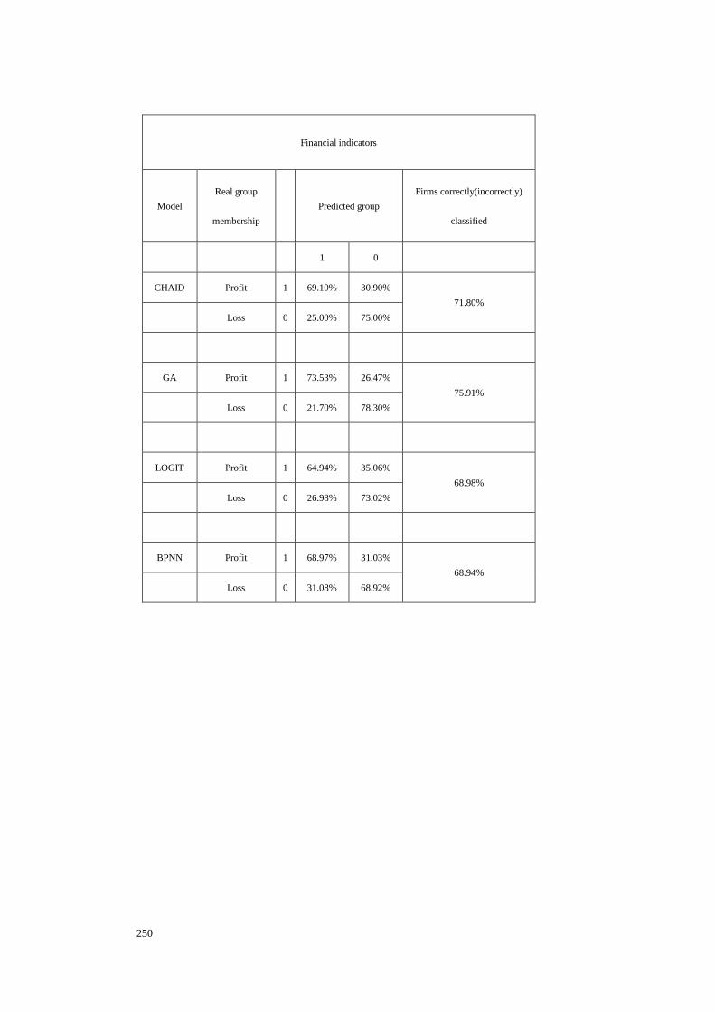
250
Financial indicators
Model
Real group
membership
Predicted group
Firms correctly(incorrectly)
classified
1 0
CHAID Profit 1 69.10% 30.90%
71.80%
Loss 0 25.00% 75.00%
GA Profit 1 73.53% 26.47%
75.91%
Loss 0 21.70% 78.30%
LOGIT Profit 1 64.94% 35.06%
68.98%
Loss 0 26.98% 73.02%
BPNN Profit 1 68.97% 31.03%
68.94%
Loss 0 31.08% 68.92%

251
Non-financial indicators
Model
Real group
membership
Predicted group
Firms correctly(incorrectly)
classified
1 0
CHAID Profit 1 31.50% 68.50%
53.70%
Loss 0 19.10% 80.90%
GA Profit 1 0.00% 100.00%
47.38%
Loss 0 1.70% 98.30%
LOGIT Profit 1 50.92% 49.08%
53.67%
Loss 0 43.59% 56.41%
BPNN Profit 1 27.59% 72.41%
41.50%
Loss 0 44.59% 55.41%
Table 6.3-a The Comparison of prediction accuracy of four data mining methods
Table 6.3-a indicated all three combinations of indicators used in this research, the
accuracy of data mining methods with different indicator groups are listed. The
information included in Table 6.3-a has been visualised in order to find the patterns
more straightforward.

252
Figure 6.3-a, The Visualisation of prediction accuracy (1)
Figure 6.3-a indicated the Accuracy of four methods. It is evident that the highest
prediction accuracy is the GA model with financial indicators. Including non-financial
indicators could increase the accuracy of prediction models was proved in CHAID and
Logit model. Although the value of non-financial indicators is not directly shown on
the GA and BPNN models, there is other evidence shows the usefulness of non-
financial indicators. Individually, in the GA models, the significant indicators in the
Financial and Non-Financial model are more than in Financial indicators group. As
previously discussed in Section 5.5.5, the GA model with financial and non-financial
indicators may be more comprehensive in explaining the features of operational and
strategic risks.
On the other hand, as discussed in Section 5.6.5.1, the BPNN model with financial
indicators did not converge to target output value, which means the predictive result
cannot be used in risk evaluation. Compared the result of BPNN model with three
different indicator groups, there is only the BPNN model with financial and non-
financial indicators converged to target output value within set iteration times.
Although the results of the ROC test and prediction accuracy of BPNN model with the
financial indicators group were acceptable, the output value cannot converge to target
0.00%
10.00%
20.00%
30.00%
40.00%
50.00%
60.00%
70.00%
80.00%
CHAID GA LOGIT BPNN
Accuracy
F and NF
F
NF

253
ranges of KPI. The overfitting problem will occur as the iteration times increased to
1000. As a result, the BPNN model provides a meaningful result only with financial
and non-financial indicators. The usefulness of non-financial indicators was examined
in four different models, which included statistical methods and non-statistical
methods. Therefore, the non-financial indicators played an important role in the
selection of KRIs in increasing accuracy, providing a more comprehensive explanation
and optimising the predictive result.
Figure 6.3-b The Visualisation of prediction accuracy (2)
Figure 6.3-b shows the prediction accuracy of the same indicator groups in the
different four models. As it shows, there is not a significant difference between
financial indicators group and financial indicators and non-financial indicators group.
The accuracy of all models with non-financial indicators group is relatively low, which
cannot be used to predict. Since the selected KPI is the firm performance, the selected
KRIs should be able to measure the firm performance well. However, only around 50%
accuracy cannot support the risk evaluation, since the tossing coin process is also with
a fifty-fifty chance. The accuracy of GA and CHAID model is similar, which is higher
than the other two models. Compared to the mechanism of two GA and CHAID model,
the CHAID model could provide information about significant indicators and the
0.00%
10.00%
20.00%
30.00%
40.00%
50.00%
60.00%
70.00%
80.00%
F and NF F NF
Accuracy
CHAID
GA
LOGIT
BPNN

254
value of the indicator, while the GA model could only provide the significant
indicators. In the risk management process, it is also important to know the treatment
of the risks, where the information of KRIs is the more, the better. Therefore, it could
be concluded that the CHAID model will be selected as the primary model since the
information provided by the CHAID model will be more than the other three models.
6.4 Result Evaluation
The Risk Treatment is to interpret the rules and patterns generated in the Risk
Assessment step, which will also be supported by Interpretation result step in Data
mining process. Based on the enterprise risk management framework, the features of
risks have been classified into four different risk catalogues. Since the two processes
have been connected via KPI and KRIs, the threshold values of KRIs could be used to
find out to reduce risks.
Figure 6.4-a Rules by CHAID models
Figure 6.4-a described the roadmaps of firms, which generated by CHAID method.
The yellow rows indicated the strong rules, which the rules could determine the firm
performance with probability around 90%. To comprehensively consider the risks, it
is necessary to find patterns and rules from all the three combinations of the indicators
for selected methods. The probability of performance good around 90% or less than

255
10% could be considered as convincible rules, which have been marked as yellow. It
could also be concluded that the variables in the rules are KRIs, which are more
important to detect the potential risk.
Furthermore, the rules generated by other methods could also be used to interpret the
result. The financial risks are the most important risk among other three risks. There
are total of six out of nine convincible rules are related to financial risks. There are
also five out of nine convincible rules are related to strategic risks, and four out of nine
convincible rules are about operational risks. All of the convincible rules are related
to financial risks, which indicated the importance of financial risks. From the Figure
6.3-a, the KRIs generated by CHAID model are net profit to equity (x31), Quick ratio
(x2), Size of firms (y19), Listed duration (y17), fixed assets to total loans (x15), long-
term liability to long-term liability and equity (x12), bank loans to total assets (x19),
environment index (y7), technology innovation index (y8) and industry (y1).

256
F and NF Estimate Std.Error z value Pr(>|z|)
x2 9.60E-02 3.80E-02 2.487 0.013 *
x4 1.40E+00 6.00E-01 2.296 0.022 *
x8 2.90E+00 6.70E-01 4.29 0 ***
x17 8.20E-01 3.80E-01 2.174 0.03 *
x31 7.30E+00 2.00E+00 3.638 0 ***
x34 -4.00E+01 5.00E+00 -8.109 0 ***
y2 3.20E-01 1.40E-01 2.299 0.021 *
y4 1.80E-02 8.00E-03 2.292 0.022 *
F x2 1.00E-01 3.91E-02 2.568 0.01 *
x5 2.21E+00 8.91E-01 2.483 0.013 *
x22 -1.83E+00 6.41E-01 -2.852 0.004 **
x23 2.59E+00 7.64E-01 3.392 0.001 ***
x31 6.15E+00 1.98E+00 3.115 0.002 **
x34 -3.79E+01 4.82E+00 -7.878 0 ***
NF y3 -1.00576 0.46441 -2.166 0.03034 *
y4 0.21761 0.10262 2.121 0.03396 *
y5 0.27097 0.1258 2.154 0.03124 *
y7 0.20449 0.09145 2.236 0.02534 *
y8 0.12651 0.0576 2.196 0.02807 *
y10 -2.31224 1.07007 -2.161 0.03071 *
y14 -0.27044 0.10283 -2.63 0.00854 **
y17 0.31125 0.15378 2.024 0.04297 *
y19 -0.19107 0.09527 -2.005 0.04492 *
Figure 6.4-b Significant indicators by LR methods
Figure 6.4-b shows the result of Logit Regression. There are eight significant

257
indicators in the financial and non-financial group, where the top three z-value
indicators are net profit to equity (x31), net profit to assets (x34) and equity to assets
(x8). There are six significant indicators in the financial group, where the most
significant indicators are net profit to assets (x34) and tangible fixed assets to total
assets (x23). There are nine indicators are significant in the non-financial group, where
the most significant indicator is a number of research staffs (y14). Although the KRIs
are significant to the KPI, the coefficient of the KRIs cannot interpret how the
importance of the indicators in measuring KPI. Since Logit regression can not generate
the threshold values of the KRIs, the rules and patterns of KRIs may not be able to
describe all aspects of the KPI.
Group Iteration Importance Accuracy Indicator Name
Financial and
non-financial
1 15.12184885 0.6269 x31 Net profit to equity
2 12.94503794 0.7265 x32 Profit before tax to equity
3 12.07511835 0.7449 x34 Net profit to asset
4 8.728316218 0.7495 x37 Gross profit /net sales
5 4.852187639 0.7517 x33 EBIT/EBT and finance expense
6 3.93329857 0.7494 x3 Absolute liquidity
7 3.574172304 0.7676 x12
Long-term liability to long-term
liability and equity
Financial
1 15.03821378 0.646844 x31 Net profit to equity
2 15.00426021 0.7378201 x32 Profit before tax to equity
3 12.30907294 0.7630796 x34 Net profit to asset
Non-financial
1 4.385605748 0.5239464 y10 Audit opinions
2 2.295658305 0.5262192 y9 Employees education
Figure 6.4-c Significant indicators in GAs method

258
Figure 6.4-c indicated the most significant indicators in all the three indicators groups
with the GAs method. The financial and non-financial group generated the most KRIs,
where the amount of the KRIs is seven. The financial group generated 3 KRIs, and the
non-financial group only has two KRIs. As discussed in Section 5.6.5, the accuracy of
the non-financial group cannot be used to predict KRI. There is less KRIs in financial
indicators group than the financial and non-financial group, which means including
the non-financial indicators could provide more comprehensive result in selecting
KRIs. Therefore, in GA models, the financial and non-financial will be the optimised
choice in the selection of KRIs, which is considered the comprehensiveness and the
accuracy.
F and NF Output_0 0.94401 0.34138
Output_1 0.05605 -0.3466
F Output_0 0.76269 -0.11104
Output_1 0.2396 0.0811
NF Output_0 0.36506 0.12428
Output_1 0.63826 -0.02857
Figure 6.4-d Converging results of BPNN models
Figure 6.4-d shows the converging results of three indicators group in BPNN models.
The KPI was coded as 0 and 1, which means poor performance and good performance
respectively. It is clear that there is only financial and non-financial group converged
to target output value, where the other two indicator groups cannot converge to 0 and
1. As discussed in Section 5.6.5, although the accuracy of financial and non-financial
indicators group is the second one, the model converged to target output indicated this
one predicted the KPI better than the other two models. Compared with other methods,
the BPNN model cannot indicate the threshold and the patterns of the KRIs. As there
is the black box mechanism built in the algorithm, it is not possible to interpret the
result with the certain rules. Therefore, in the BPNN models, the prediction accuracy

259
is not the most important aspect, while the converged value and accuracy should be
considered at the same time.
After compared all four models with three different indicator groups in addressing the
KRIs and KPIs problems, the optimum algorithm is CHAID method, which provided
the second highest accurate prediction and threshold values of KRIs. Although the
CHAID is better than other algorithms, it is necessary to consider the results of other
algorithms to get the most comprehensive view. To sum up, the roadmaps and
threshold values were described as follow: to achieve good performance, the listed
SMEs in China can follow such rules:
1. Net profit to equity greater than 0.12 and quick ratio greater than 0.447
2. Net profit to equity greater than 0.2 and firm size (log) greater than 21.278
3. Net profit to equity less than 0.014 and inventory to current assets less than 0.363
4. Net profit to assets has a native effect on firm performance, and the research stuff
is important to firm performance
5. Profitability and liability are the most important aspects generated by GA
algorithms, while the employee education and audit opinion are critical non-
financial indicators in GA algorithms
6. The profitability ratios, liability ratios, firm size and Goodwill and intangible asset
are essential aspects, which are belonging to financial risks, operational risks and
strategic risks.
6.5 Hypotheses Verification
There are eight hypotheses have been purposed to verify the DM-RM model. The
hypotheses were listed below:

260
No. Research Hypotheses
H1 The data mining process and risk management process could be synchronised together
to achieve risk management purposes.
H2 The ERM framework could be embedded in the risk management process.
H3 The usage of KPIs and KRIs complied with the ERM framework and can improve the
risk management process
H4 Combining financial and non-financial indicators in the selection of KRIs can explain
most of the features required by the enterprise risk management framework.
H5 Non-financial indicators are essential in the whole risk management process.
H6 The early warning system could provide solutions for KRIs in the risk treatment step.
H7 The business intelligence approach can help the ERM framework become embedded
into the risk management process.
H8 The business intelligence approach can enhance the ability to capture useful
information to be used as indicators in the risk management process for SMEs.
Table 6.5-a The Summary of hypotheses
Table 6.5-a shows the contents of eight research hypotheses. The hypotheses attempted
to examine the relationship between the data mining process and risk management
process. KPIs and KRIs have linked the data mining process and risk management
process. Also, the ERM framework, EWS, BI and SMEs have also been examined.
The value of non-financial indicators in DM-RM model has also been tested.
Figure 3.3-c shows the connections with hypotheses in DM-RM model discussed in
Section 3.4. The results were recalled verifying the hypotheses. There are total eight
hypotheses were initially proposed as follow:
H1: If the data mining process and risk management process could be synchronised
together to achieve risk management purposes.
H2: The ERM framework could be embedded in the risk management process.
H3: The usage of KPIs and KRIs complied with the ERM framework and can improve
the risk management process
H4: Combining financial and non-financial indicators in the selection of KRIs can
explain most of the features required by the enterprise risk management framework.
H5: Non-financial indicators are essential in the whole risk management process.

261
H6: The early warning system could provide solutions for KRIs in the risk treatment
step.
H7: The business intelligence approach can help the enterprise risk management
framework become embedded into the risk management process.
H8: The business intelligence approach can enhance the ability to capture useful
information to be used as indicators in the risk management process for SMEs.
The H1 is the foundation of this study. In order to test H1, the results need to show the
data mining process and risk management process have been integrated together.
There are three main steps in the RM process (ISO 31000, 2009). Moreover, there are
five data mining steps (Han et al., 2012). The connections were shown below:
Figure 6.5-b Flowcharts of DM-RM model with hypotheses
Figure 6.5-b shows the explicit connections between the DM process and risk
management process. It is clear that each sub-step was synchronised by using KPIs
and KRIs. If the KPIs and KRIs were found and meaningful, it indicated that the two
processes had been integrated. The results of the data mining methods have found out
the KPI and KRIs, where the usefulness and meaningfulness of KPI and KRIs have

262
also been proved. Therefore, if the usage of KPI and KRIs was successful, the H1 can
be proved. From the empirical view, the results of DM should support the RM process,
which means the feature selection functions should be effective. As discussed in the
previous section, the overall prediction accuracy is over 75% for all models, it means
the two different performance groups can be distinguished by using DM methods in
this study. As a result, the empirical evidence supports that the DM process can be
integrated to the RM process.
For H2 examined, it is necessary to specify the risk catalogues mentioned in the ERM
framework, and the results should also follow the ERM framework. The four risk
catalogues under the ERM framework (CAS, 2003; Verbano and Venturini, 2011) have
been applied in order to capture all the risk features. In Section 4.4, the information
was collected based on the risk catalogues under the ERM framework. Meanwhile, the
indicators have been calculated upon the ERM framework as well. In Section 5.7, the
results of four different data mining methods have been verified, which indicated that
the results are meaningful and reasonable. Moreover, the empirical findings in Section
6.4 illustrated that the four different risk types are all important in the RM process.
The results from the CHAID model directly show the connections and importance
between rules and risk types. Therefore, the H2 has been proved that the ERM
framework has been embedded into the RM process.
The H3 examined the effectiveness of using KPIs in the DM-RM model. The KPIs
aimed to provide measurements for the research targets. The KPIs have been used in
‘Establish the Context’ step in the RM process, where the purpose of the RM process
was specified. In Section 5.3.4, the usage of different KPIs (Altman’s Z-score and
ROA) has been compared. Based on the empirical results, the ROA has been selected
as KPI in this study. Verbano and Venturini (2011) stated that the ERM aims to
maximise the firms’ value. The ROA directly measured the performance of the firms,

263
which was used by other studies as well (Altman et al., 2010; Heikal et al.; 2014). Also,
the selection of KRIs is also complied with the risks features by ERM framework.
Since the KRIs determined the prediction accuracy of KPIs, the KPIs are also based
on the ERM framework. The data mining methods helped in reducing the number of
indicators that decision-makers need to focus, which means the efficiency of the whole
RM process has been simplified. Therefore, it concluded that the usage of KPIs
enhanced the efficiency of the RM process and complied with the ERM framework.
The H4 required that both a financial indicator and non-financial indicators were
applied in data mining methods, where the results required proving the value of non-
financial indicators. In the applied four data mining methods, there were three different
indicators groups (financial and non-financial; financial; and non-financial) indicators
have been applied in order to verify the value of non-financial indicators. In Section
5.3 to 5.6, each data mining method applied three different indicator groups. It
concluded that the non-financial indicators are essential in the DM-RM model,
because including non-financial indicators can increase the accuracy of the prediction.
However, as stated in Section 6.4, the non-financial indicators cannot solely predict
the performance. Using financial and non-financial indicators together is necessary.
On the other hand, the results indicated that the financial indicators could not explain
some of the characters of strategic risks and hazard risks. The usage of non-financial
indicators considered the aspects that financial indicator cannot explain. The
effectiveness and meaningfulness of using non-financial indicators were thoroughly
discussed in Section 6.4. Also, because the prediction accuracy of all models is over
75%, it means the results are meaningful. Especially, the KRIs were selected from
financial and non-financial indicators, which proved the usefulness of the indicators
in the whole RM process. Therefore, with over 70% accuracy, the financial and non-
financial indicators could be used to explain the risk features under the ERM
framework.

264
H5 examined the usefulness and meaningfulness of non-financial indicators in the
model. The non-financial indicators were generated based on the risk catalogues in
ERM framework by CAS (2003), where some information was transferred into
indicators based on the understanding of the risk features. As discussed in Section 6.3,
the prediction accuracy increased as non-financial indicators included in the CHAID
and Logit regression models. In the GA method, the non-financial indicators can
provide a more comprehensive view of the KPI, which takes four more indicators into
account. In the BPNN model, only the financial and non-financial indicators group
could converge to the target result. However, the result also proofed that the non-
financial indicators cannot independently predict the KPI as KRIs. Since the selected
KPI should clearly state the financial position of firms, the KPI is more like a financial
indicator. As a result, the non-financial indicators cannot explain the feature of
financial indicator makes sense, where the result of prediction accuracy with non-
financial indicators group is acceptable. Although the non-financial indicators cannot
predict KPI independently, it still can proof the usage of non-financial indicators is
meaningful and useful.
To examine H6, the usefulness of EWS required to be proved. The EWS monitored
and reported alerts of the potential risks (Koyuncugil and Ozgulbas, 2012). In the risk
treatment step in the RM process, the EWS provided explanations of rules and patterns
found by the data mining process. Risk treatment thus also includes improving the
existing control methods and developing new controls (ISO 31000, 2009). As
discussed in Section 6.4, the threshold values provided the specific ranges of KRIs in
good and poor performance firms. If the decision makers followed the path of KRIs in
good performance firms, the effect of risks would be reduced to a minimum level. As
stated in Section 6.4, there are several convincible rules have been found out. The RM
roadmaps for the SMEs have been developed. If the ratios in convincible rules were

265
reached, it means the performance will be in danger or getting better. As a result, the
EWS provided solutions for controlling risks by improving KRIs.
To verify H7, the usefulness of BI approach in helping the ERM framework for RM
process required to be proved. The BI approach suggested that the information could
be anything useful, which may be obtained from websites, reports, emails, etc., while
the non-financial indicators generated by the BI approach considered this information.
Most of the aspects described by the ERM framework were considered with the non-
financial indicators generated by the BI approach. The BI approach provided solutions
in data collection, data clean up and data transferred. As discussed in Section 6.4, the
KRIs have been selected from all indicators, the effectiveness of the data mining
methods has been confirmed. Therefore, the BI approach can help the ERM
framework by providing candidates of KRIs, which was embedded in the RM process.
To examine H8, the functions of the BI approach in data collection required to be
specified. This study has collected 849 listed Chinese SMEs in the Shenzhen Stock
Exchange. There are forty-two financial indicators, and nineteen non-financial
indicators were collected from each frim. The BI approach provided solutions in
transferring information into indicators (Chen et al., 2012). The useful information can
be transferred into indicators upon the requirements by ERM framework, which has
been discussed in Section 6.4. Since the prediction accuracy is acceptable, the DM-
RM model for SMEs is successfully developed. Also, the risk features of SMEs have
also been captured by analysing the indicators provided by the BI approach. As a result,
the BI approach provided solutions in transferring information into data, which
captured the risk features of SMEs.
No. Result Explanation
H1 Verified The model prediction accuracy over 70%
H2 Verified ERM risk types covered most of the features

266
H3 Verified KPIs and KRIs have been selected and can be used to predict
H4 Verified
The FIs and Non-FIs can do feature selection with over 70%
accuracy
H5 Verified
Including both FIs and Non-FIs can increase the prediction
accuracy
H6
Partly
Verified
The rules and patterns can build a roadmap for SMEs, but can
be improved with more information
H7 Verified The indicators can be visualised by using BI approach
H8
Partly
Verified
The information can be quantised by using the BI approach,
but can be expanded
Table 6.5-b Hypotheses verification
Table 6.5-b shows the hypotheses verification. All the eight hypotheses have been
thoroughly discussed above, where each clarification of each hypothesis has also been
provided. This study shows the detailed steps in integrating the RM process and DM
process. Meanwhile, as shown in Figure 6.5-b, all connections among all the
components have been linked with hypotheses. Meanwhile, the quantised
measurements of the model performance have shown, which illustrated the prediction
accuracy of DM methods. Three combinations of data groups have been compared,
where the value of non-financial indicators has been recognised. Furthermore, the
most suitable DM method for RM in SMEs has been found out by comparing the
comprehensiveness and accuracy of the prediction. On the other hand, the BI approach
and EWS can be improved by using broader information and more systematic
framework, which means these two components can be improved. Therefore, all the
hypotheses have been verified.
6.6 Comparison with other studies
The data mining methods in financial distress prediction is a classic topic. Geng et al.
(2015) stated that the statistical techniques were commonly applied in the prediction
of this area. However, due to the unrealistic assumptions, some of the statistical

267
methods may not perform well in the area. Some scholars used Logit regression to
overcome the drawbacks of traditional statistic methods, while others tried to use
machine learning methods based on artificial intelligence. Geng et al. (2015) stated
that researchers applied neural network (Fletcher & Goss, 1993; Wilson & Sharda,
1994), decision trees (Frydman, Altman, & Kao, 1985), genetic algorithms (Shin &
Lee, 2002). In this research, the data mining methods: LR, CHAID, GAs and NN were
applied, which were used to build the integrated model to manage risks. The main
purpose of DM-RM model is to select KRIs to determine KPI, which is used to link
the data mining process and risk management process. Therefore, these data mining
methods were purposed to find out KRIs based on KPI to support the whole framework,
which means these methods focused on the feature selection aspect.
The prediction accuracy of the DM-RM model has also been compared with other
studies. According to Geng, et al. (2015), the most accurate model is Neural Network
in their research, where the accuracy is around 78%. Shin and Lee (2002) applied the
GA method to predict bankrupt, where the accuracy is about 80%. Gordini (2014)
stated that the accuracy of GA, SVM and LR were 78%, 77.2%, 72% respectively.
Since the purpose of studies may not be the same, some of the research will not only
focus on the prediction of firm performance to achieve risk management process.
Compared with other studies, the result of this research is about 77% accuracy with
four different methods, which is not entirely different from other studies. Therefore, it
is possible to conclude that the result of this research is acceptable in the academic
aspect.
6.7 Summary
This chapter evaluated the result of all methods applied in this research, verified the
constructed framework, and compared the result with other methods. The main finding

268
is that there are connections between KRIs and KPI, which could be used to link the
data mining process and risk management process. Furthermore, the selection of KRIs
and KPI provided evidence that the ERM framework could be used to risk
management process. The successful usage of KRIs and KPI also proved that the
meaningfulness and usefulness of two different processes. Meanwhile, the value of
non-financial indicators has also been verified, which was clearly described by the
comparison of different methods. Furthermore, the CHAID model provided the
roadmap and threshold values of KRIs, which is complied with the idea of the early
warning system. The ERM steam was also explained by the model, where the rules
generated by the four models followed the risk catalogues classified by the ERM
framework. Additionally, the result of this research was also compared with other
studies in order to verify the meaningfulness and robustness of models. Since there is
not a significant difference between the result of this research and other scholars’ work,
it is concluded that the result is acceptable and useful.
This section has discussed the results of four different data mining methods. It detailed
introduced four data mining methods for KRIs selection. In general, the results
obtained from this study empirically suggested that the data mining process and risk
management process has been combined. The results also supported that the usage of
KPIs and KRIs is successful, where the KRIs have been selected upon the selected
KPI. The DM-RM model also successfully embedded with ERM framework in risk
identification; EWS in risk treatment; BI approach in data collection and SMEs in data
selection.
The results of this study also supported that the usage of non-financial indicators is
essential to building the DM-RM model for SMEs. It has been proved that the non-
financial indicators can provide supports to financial indicators.

269
7. Conclusion
The study aims to improve the risk management process with the data mining process.
In doing so, it incorporated the data mining process with ERM framework, BI
approach, EWS and SMEs as components. This study also examined the usage of KRIs
and KPIs in addressing risk management to capture all the risk features. Also, the study
also examined the value of non-financial indicators in the risk management process.
The DM-RM model was developed in this study, which can consider all the risks
together in order to improve the firms’ performance purposively. The study has also
introduced the importance of risk management and discussed the four types of risks
based on the ERM framework by CAS in 2003. The study also made initial attempts
in the integrated risk management process with the data mining process and
successfully concluded the listed SMEs in China can be grouped based on the
performance.
The purpose of this chapter is to provide a conclusion of the study. The chapter
discussed how the study’s aim and objectives are achieved; outlined the theoretical and
practical contributions; identified the limitations of this study; and provided
recommendations for future research.
7.1 Overview
This study has combined the data mining process and risk management process and
concluded a method in the application of KPIs and KRIs by BI approach for SMEs.
The ISO and COSO risk management framework provided a solution for improving
the efficiency of the risk management process. The risks are required to be detected
and identified in the risk management process, which required detailed practical
guidance. However, the ISO framework only provided the brief process in the risk
270
management, which included the build the context, risk assessment and risk treatment.
In order to achieve risk management goals in daily operating, it is necessary to explain
more specific guidance in risk management. The COSO framework gives the
management prototype of the framework in their risk management activities, which
includes control environment, risk assessment, control activities, information and
communication and monitoring activities. In order to apply an enterprise risk
management framework in firms, there should be more practical guidance from the
theory of enterprise risk management (Nocco and Stulz, 2006). The enterprise risk
management framework has been studied by many scholars (Verbano and Venturini,
2011), which considers both financial and non-financial aspects of firms’ operation.
Verbano and Venturini (2011) claimed that enterprise risk management is one step
further from traditional financial risk management. O’ Donnel (2005) pointed out that
the strategies, market, processes, financial resources, human resources and
technologies were all structured into enterprise risk management. To measure all
aspect of firms operation, the application of only financial indicators is not enough.
As a result, the non-financial indicators have been suggested and developed to improve
the risk management process. This study developed the DM-RM model with the ERM
framework, BI approach, EWS, and SMEs components. The usage of data mining
process will also be discussed and recommend other studies in different areas.
7.2 Achievements of aims, objectives and research questions
This section reviews the aims, objectives and research questions presented in Chapter
1 in order to verify that they have been achieved. The research aim is:
To investigate how financial and non-financial indicators can be used in risk
management procedures with the data mining process based on ERM framework by
applying a BI approach for SMEs.

271
The aim has been achieved. Chapter 2 has introduced the relationship between other
concepts and financial and non-financial indicators. Chapter 3 has thoroughly
discussed how to use financial and non-financial indicators in the proposed DM-RM
model. Since the usage of non-financial indicators is a recent development, there are
many scholars have proposed to apply it with their existing financial indicators
research (Geng et al., 2015; Koyuncugil and Ozgulbas, 2012). To use non-financial
indicators in the models, it is necessary to apply BI approach to capture the information
required in the ERM framework by CAS (2003). On the other hand, practical guidance
was obtained as the DM-RM model has been successfully built. As discussed in
Chapter 5 and 6, the result of the data mining process could support that the model is
valid. Therefore, the step-by-step practical guidance was obtained, which was shown
by the process of model development.
There are also six detailed research objectives:
1. To develop a risk management process with enterprise risk management
framework and data mining process.
2. To measure risks with both financial and non-financial information by using a
business intelligence approach.
3. To comprehensively consider the risks applicable to the enterprise risk
management framework and to integrate all necessary risk management and data
mining steps for this consideration into one model.
4. To examine different data mining methods that can be applied in the analysis of
the risk management process in SMEs.
5. To evaluate the usefulness of non-financial indicators in the risk management
procedure.
6. To establish a robust early warning system to predict the likelihood and impact of
different kinds of risks for SMEs based on financial and non-financial factors
using data mining methods.

272
Chapter 2 and 3 reviewed concepts in the risk management process and data mining
process, which introduced the fundamental components of the theoretical framework.
Furthermore, the two chapters also discussed the usage of BI approach in capturing
non-financial indicators, which could support the risk catalogues by ERM framework.
Meanwhile, since the theoretical framework was developed and verified in this
research, the model could comprehensively explain all the four risks under the ERM
framework in one-step. Chapter 5 and 6 discussed different data mining methods in
KRIs selection, which also provided an insight view of the risk management process.
In Chapter 6, the total of four different methods applied in this research were compared
with each other to evaluate the prediction results. Also, the prediction results also
indicated the usefulness of non-financial indicators. Since the added non-financial
indicators could either improve the accuracy or indicate more KRIs, it could be
concluded that the non-financial indicators are usefulness in this research. Finally, the
early warning system could be built via the rules and patterns found in Chapter 5 and
6. The threshold values and significance of KRIs could be generated with all four
models, which could provide the essential components of building an early warning
system. As a result, the early warning system could be built with the results gathered
in this research.
The aim and objectives of this research were used to address six research questions:
1. Is it possible to use the risk management framework in SMEs by using Enterprise
risk management framework?
In order to address this question, it is important to obtain the prediction result based
on the ERM framework, which indicates the risk positions of the target firms. Since
there are different types of risk management framework (Verbano and Venturini, 2011),
it is necessary to specify the risk management framework. After that, the risk
catalogues of the risk framework should be followed in the whole risk management
process. In this research, the risk management process is followed the ERM

273
framework. Also, the database is selected from the listed Chinese SMEs, which is also
complied with the question.
2. How to conduct the risk management procedure under the enterprise risk
management framework with business intelligence approach?
According to Han et al. (2012), the data mining process could use BI approach to
generate data and build a database. Under the ERM framework, there are total of four
different risk catalogues, which cannot be fully covered by financial indicators only.
As a result, it is necessary to use some non-financial indicators to explain features of
all risks. Since BI approach could support the data collection step, it is possible to
gather enough information and transfer information to indicators to complete the risk
management process.
3. Is the business intelligence approach useful in quantising and standardising the
information into indicators?
The BI approach is useful in transferring the information to data, where the
information gathered from Websites and other reports could be used in the data transfer
step. Han et al. (2012) stated that the data mining process includes data cleaning up
and data transferring steps. The raw data required to be cleaned and transferred before
it becomes indicators that could be directly used in the model. The BI approach could
be used to clean up and transfer the data format via coding or software. Therefore, the
question could be answered, since BI approach provided supports to quantising and
standardising the data.
4. How to use financial indicators and non-financial indicators in the prediction
models to capture the risks under the enterprise risk management framework?
The financial indicators and non-financial indicators could be used as input indicators
in data mining methods. Since there are four different risk catalogues in ERM

274
framework suggested by CAS (2003), the indicators should cover financial risks,
operational risks, hazard risks and strategic risks. As discussed in Section 4.4 and
Section 5.2.1, the indicators are collected from the risk catalogues by CAS (2003).
Since selected indicators could cover most of the features mentioned in the ERM
framework, it is true that the indicators could capture most of the features. Therefore,
the question could be solved, since the indicators were developed based on the
requirements by ERM steam.
5. Are the non-financial indicators helpful in the promising model to measure firm
performance? If yes, how much can it help?
In order to address this question, it is necessary to use at least two groups of indicators,
where the results of financial indicators and non-financial indicators should be able to
be compared. As discussed in Chapter 5 and 6, there are total of three different
indicators groups, which are financial and non-financial indicators, financial
indicators only and non-financial indicators only. The prediction accuracy could be
used as the measurements of each indicator group. As discussed in Chapter 6,
including non-financial indicators in the model could increase the prediction accuracy
or increase the range of KRIs selection. The detailed discussion about how much non-
financial indicators can help was listed in Section 6.4. Therefore, it can prove that the
non-financial indicators are helpful.
6. Could the BI approach and the enterprise risk management framework integrate
together in addressing risk management in SMEs?
In order to address this question, it is necessary to find out the function of BI approach
in the risk management process and ERM framework. As discussed in Chapter 2 and
4, the BI approach could gather risk features required by the ERM framework. Also,
the risk management process is required to follow one of the frameworks (Verbano
and Venturini, 2011), where the ERM framework would be more suitable for this

275
research. The important thing is to capture enough information require by ERM
framework to complete the risk management process. The BI approach will provide
information to support ERM and not limited to specific risk frameworks. The ERM
framework provides risk catalogues for the risk management process, which limited
the range of indicators selections. The ERM framework and BI approach played
different roles in the whole risk management process. As a result, it is necessary to use
both the ERM framework and BI approach in this research to complete the risk
management process.
The decision makers may concern how to improve the performance and reduce the
uncertainty. In section 6.4, the advantages of each method were discussed, which could
be selected by decision makers. In order to reduce risks, the decision makers could
control the ranges of KRIs or monitor the values of KRIs in order to improve the
performance, which is complied with the purpose of risk management mentioned by
Verbano and Venturini (2011). Furthermore, as discussed in Chapter 3, the purpose of
this model could be changed upon required, which could provide more broad
applications for different decision-making processes. The scholars may concern the
implementation of data mining process into other areas. The data mining process can
be easily adjusted based on a general purpose in another area, which will be used to
find hidden rules and patterns. The BI approach in data mining process provided
supports in data collection and data clean-up, which can be used in collecting data for
other areas and topics. Also, the embedded ERM framework and usage of KPIs and
KRIs provided a more comprehensive view of the risk management process, which
improved the efficiency and coverage for the current knowledge. Therefore, these
questions provided theoretical extension and practical guidance of the developed
model in this study, which was answered by the discussion in section 6.4.

276
7.3 Contributions
7.3.1 Theoretical Contributions
Although the study in risk management started decades ago, the risk management is
still a relatively new topic in SMEs, especially with the data mining process and BI
approach. By providing empirical evidence on the enterprise risk management
amongst SMEs in China, the study contributes to risk management literature by
integrating numbers of processes and concepts from risk management, enterprise risk
management, early warning system and business intelligence. Specifically, this
research combined risk management process and data mining process and built a
comprehensive framework to improve the current risk management process. Although
the combination of the data mining process and risk management process was
attempted before (Johnson, 2010), but the use of standard risk management process is
the first time. The attempt of combing the data mining process and risk management
process is a new area, which provided a different view of the data mining process.
Furthermore, the application of ERM framework in risk management for SMEs is also
be developed, which was considered understudied by Verbano and Venturini (2013).
The total risk process and four risk types were fully considered in this study, which
followed the ERM framework (Verbano and Venturini, 2013). As a result, this study
provides a boarder view extended from existing literature by combining risk
management process with the data mining process, with ERM, BI and EWS.
The business intelligence approach provided the support in data collection and
indicator selection for the data mining process. This study followed the ERM
framework in SMEs risk catalogues, which has developed the risk indicators under
four risk types claimed by CAS (2003). Furthermore, this study extends the enterprise
risk management framework by applying business intelligence concepts. It solved the
problem of building up database, which provides the foundation of a data mining
277
process. It has contributed to the current risk management process in model selections,
variable selections and methods integration. In the studies of Chinese listed firms,
many scholars applied ST and non-ST as a classifier. Differently, in this study, the
classification did not follow the ST and non-ST classification, while the classifier was
objectively selected by using statistical methods. This study also tried to provide the
dependent variables other than ROE in other studies and attempted to provide more
dimensions to explain the risks faced by SMEs. The study considered all the risks in
an integrated framework rather than analysing the risks separately, which could
provide a more comprehensive view of decision makers. As stated by Verbano and
Venturini (2011), most of the studies did not cover all of the four risk catalogues, since
collecting all the information required by the ERM framework is relatively tricky.
However, this study attempted to capture all the risk features mentioned in the ERM
framework and achieved acceptable prediction accuracy. The use of EWS in the DM-
RM model has successfully found the convincible rules from all the rules and patterns
and detected the warning signals. It indicated that the EWS was integrated into the risk
management process and data mining process. Therefore, it concludes that this study
has contributed to this topic and expanded the data mining process to other similar
areas.
7.3.2 Practical Contributions
The findings contribute to the SMEs in China as well as broader risk management
participants in other areas and industries. The developed process of building the
integrated DM-RM model provides detailed steps for using the data mining process.
Additionally, the data mining process has been developed based on the risk
management process, which means the purpose of the data mining process is defined
by the purpose of the risk management process. For a specific research target, it is
possible to apply the DM-RM model to build a specific model, which was used to find

278
potential rules and patterns for targeted objectives. This study thoroughly discussed
the steps for risk management and the essential steps in decision-making. It specified
the necessary steps in integrating data mining process and risk management process,
which required symmetrically developed.
The risk management process provides the targets and goals for the data mining
process, which resulted in closer connections between the two processes. It also
proved that risk management would require more complex and integrated methods to
find the benchmarks to avoid business failure. It also proved that a data mining method
might not provide full explanations of the ERM framework since the risk features can
be insignificant with different data mining methods. The study provided a detailed
variable selection based on the four types of risks. Moreover, it is also possible to
conduct models with different catalogues of risks. It also suggested that the difference
between good performance and poor performance enterprises may not only depend on
the financial ratios. This study also provided a different view in listed Chinese SMEs,
which did not apply ST/Non-ST classification as many previous studies (Xie and Me,
2013; Geng et al., 2015). The classification was completely objective, which comes
from the results of statistical data mining methods. This study has successfully avoided
using imbalance database (Xie and Me, 2013), where the Non-ST firms are much more
than ST firms in the imbalance database. It indicated that the ST and Non-ST is not
the only classification rule in the studies of listed Chinese SMEs.
Meanwhile, the KPI and KRIs under different risk catalogues were redefined, which
provided more accurate predictions and more efficient monitors in the whole process.
The use of BI approach collected the information from annual reports, and government
reports, which transferred useful information into indicators. The BI approach
provided more abundant information on the requirements of the risk framework. The
use of EWS efficiently explained the rules and patterns generated by data mining

279
methods. Based on the ERM framework, the rules and patterns were obtained by risk
catalogues, which provides a more specific view of the risk management process. The
convincible rules, significant variables were concluded in Section 6.4, where the
warning signals and desired trends were generated by EWS. It thus indicated that the
EWS supported risk treatment in the risk management process and result interpretation
step in the data mining process. At last, the study also allowed the companies to
benchmark themselves to their peers and competitors across different KPI and KRIs.
7.4 Limitation
This section identifies three critical limitations to this research, based on the
knowledge of the subject, the availability of time, access to information and skills.
⚫ Confining information to create indicators
There are total of four aspects of risk catalogues defined by ERM framework, which
includes hazard risks, financial risks, operational risks and strategic risks. Since the
study of financial risks and operational risks are the primary interest of the previous
studies (Verbano and Venturini, 2013), this research tried to capture the features of
hazard risks and strategic risks. Although the information was tried to collect as much
as possible, there are still some areas may not be covered. Specifically, the theft and
other crime, personal injury in Hazard risks can only be explained by geographic
information provided by firms. Similarly, the Disease and disability and Liability
claim can only be described with the closest indicators that could be found in the
reports, web information or annual reports. For strategic risks, there are also some
features could not be perfectly captured by using existing information as well.
Therefore, the result may be improved by using more appropriate indicators to
describe the features listed in the ERM framework.

280
⚫ Possible more data mining methods
Although there are total of four different data mining methods were used in this
research, it is possible to apply more data mining methods to select KRIs more
comprehensively. Other studies are using different methods to select KRIs, Rough set
analysis (Xiao et al., 2012); Clustering methods (Chen, 2013); Support vector
machines (Geng et al., 2015). Although section 6.6 discussed the results of this
research and other studies, it is possible to include more data mining methods to show
the difference of methods directly.
⚫ Limited sample size and access to information
This research analysed over 800 listed Chinese SMEs. However, as the big data study
developed, the sample size could be increased as many as possible in order to train the
model. Furthermore, since the data of unlisted SMEs in China cannot be directly
obtained by researchers, this research only publicly available data to build a database.
It is true that the listed SMEs takes only a small portion of all SMEs all over the world,
which means the rules provided by this database cannot explain part of the risk
management process among SMEs.
Although there are some limitations to this research, the researcher has attempted to
minimise the effects of the limitations. As discussed in Chapter 4 and 5, the variable
selection was attempted to capture as much information as it can, which covered most
features required by the ERM framework. Furthermore, as discussed in Chapter 6, this
research has already completed the tasks of the framework, which means currently
applied data mining methods are somehow enough.
7.5 Recommendation
Further research could be applied in several aspects based on the result of this research.

281
Firstly, the study targets may be not limited to SMEs. Since the DM-RM model has
been developed, the purpose of the model could be changed upon the users. The
research questions could then expand to other topics as long as the purposes are similar
to this research. Since Verbano and Venturini (2013) stated that risk management in
SMEs is understudied, there might be other aspects of risk management are
understudied as well. As a result, the model could be used in other risk management
related topics. Secondly, the usage of non-financial indicators could be developed. As
many scholars stated, the non-financial indicators are useful in the prediction of firms’
performance. This study has examined the usefulness of the non-financial indicators.
However, the non-financial indicators are based on the ERM framework. As Verbano
and Venturini (2011) stated that there are other risk management frameworks, it is
possible to expand the usage of non-financial indicators to other topics. Furthermore,
there is not a standard range of non-financial indicators. The range of non-financial
indicators could be different from this research to cover different features.
Further research could focus on the selection of non-financial indicators to develop
the universe ranges of non-financial indicators applied in risk management related
topics or other topics. Thirdly, the usage of data mining method to deal with large data
sample could be expanded to other topics in management academic studies. Since the
data mining method could found hidden rules and patterns from the database, it is
possible to collect related data and find out potential connections in other areas. As the
development of data mining methods, there might be other frameworks could be
combined with the data mining process to gather more rules and patterns from existing
findings. Finally, the comparison of different data mining methods could be applied.
There are many different data mining methods based on different theories. Although
the popular data mining methods were used in this research, there are still many
methods could be used, such as SVM, MV, etc. For a certain database, the different
method may conclude a similar result with a slight difference, which could be used to

282
find out the insufficiency of applied methods. Other scholars have made a similar
comparison as well, such as Geng, et al. (2015) applied three methods to predict
financial distress. Therefore, there are still many possible areas could be developed
from this research, which may produce a better understanding of the risk management
process and data mining process.
7.6 Summary
The final chapter has drawn upon the thesis to conclude the study. Some findings in
this study have been summarised, which led to several practical and theoretical
contributions. The development of DM-RM model provided a combination of risk
management process and data mining process. There are many scholars supported that
risk management process could effectively deal with risks (Cumming and Hirtle 2001;
Liebenberg and Hoyt 2003; Miccolis and Shah 2000). The developed model provides
the theory of how to assess risks after the purpose of risk management was settled. It
concluded the four different types of risks, which gives decision makers and scholars
the research direction of variable selection. Followed the catalogues by ERM
framework, the indicators have been classified and clustered within specific risk type.
If the decision makers followed the DM-RM model, the efficiency of the process
would be improved.
This study has built DM-RM model with the data from listed SMEs in China, followed
the ERM framework; and provided practical guidance in details. The predictive results
verified the accuracy of the model. The usefulness of financial factors and non-
financial factors was studied and examined in the model, where both financial and
non-financial indicators were selected as KRIs. This study also compared different
data mining methods in the selection of KRIs. The whole process of risk management,
such as variable selection; risk indicators filtering; and risk identification, was studied

283
and explained in details. As BI developed, the decision makers can get information
from structured and unstructured data by using the idea of a business intelligence
system (Negash, 2004). In order to consider risk features, this research has used forty-
two financial indicators and nineteen non-financial indicators. This study achieved
data mining methods by using SPSS, and the R Programming, which finally selected
CHAID model as the best approach. By using the data mining methods and other tests
(ROC and variable importance), the DM-RM model has successfully found out KRIs
from risk indicators and made the sequencing of four types of risk.
Moreover, the usage of non-financial risk indicators increased the accuracy of the
model, which has been proved the usefulness of non-financial indicators in SMEs. The
roadmap for improving firm performance was developed by finding threshold values
of KRIs, which is compiled with EWS. Since this study provided a solution to improve
the risk management process, the DM-RM model can be used in other related topics
that can be applied data mining process. This chapter was closed by discussing the
main findings and recommendations for further study areas.

284
8. Reference
ACCA, 2017, COSO Enterprise Risk Management Framework, ACCA,
www.accaglobal.com
Adriaans, P.W. and Zantinge, R., 1996, Data mining. Addison-Wesley, 1996.
Alexander, A.G., 2017, Enterprise risk management and business continuity,
continuity central.com.
Altman, E.I., Sabato, G., 2007. Modeling credit risk for SMEs: Evidence from the US
market. Abacus 43,332–357.
Altman, E.I., Sabao, G., Wilson, N., 2010. The value of non-financial information in
small and medium-sized enterprise risk management. Journal of Credit Risk 6 (2), 95–
127.
Altman, E.I., Narayanan, P., 1996. Business failure classification models: an
international survey, Working paper series, 1996.
Alquier, A.M.B., Tignol, M.H.L., 2006. Risk Management in Small and Medium-
sized Enterprises. Production Planning & Control, 17(3), 273-282
Akaike, H., 1987, Factor analysis and AIC, Psychometrika, September 1987, Volume
52, Issue 3, pp. 317–332
Andersen, T.J., 2008. The performance relationship of effective risk management:
exploring the firm-specific investment rationale. Long Range Planning 41

285
(2), 155e176
Arnott, D., & Pervan, G., 2008. Eight key issues for the decision support systems
discipline. Decision Support Systems, 44(3), 657-672
Arora P., Deepali, and Shipra V.,2016, Analysis of K-Means and K-Medoids
Algorithm For Big Data”, International Conference on Information Security & Privacy,
India, Science Direct, Vol. 78, pp. 507-512, 2016.
BBA – British Bankers’ Association, International Swaps and Derivatives Association,
Price water house Coopers LLP, 1999. Operational risk: the next frontier, RMA,
Philadelphia.
Beaver, W., 1967,Financial ratios predictors of failure. Empirical research in
accounting: selected studies 1966, Journal of Accounting Research, Supplement to
Vol. 4, 1967, pp.71-111.
Bajo J., Borrajo M. L., De Paz J. F., Corchado J. M., Pellicer M., 2012. A multi-agent
system for web-based risk management in small and medium business. Expert
Systems with Applications, Volume 39, Issue 8, 15 June 2012, Pages 6921-6931
Back B., Laitinen T., Sere K., 1996, Neural networks and genetic algorithms for
bankruptcy predictions, Expert Systems with Applications, Volume 11, Issue 4,
1996, Pages 407-413, ISSN 0957-4174,
Barrieu, P., El Karoui, N., 2004. Optimal derivative design under dynamic risk
measures. In Mathematics of Finance, Contemporary Mathematics.

286
Beasley, M.S., Clune, R., Hermanson, D.R. (2008). The impact of enterprise risk
management on the internal audit function, Journal of Forensic Accounting,
Becchetti, L., and Sierra J., 2002. Bankruptcy risk and productive efficiency in
manufacturing firms. Journal of Banking and Finance 27, 2099–2120.
Berman, K., Knight, J., Case, J., 2006. Financial Intelligence: A Managers Guide to
Knowing What the Numbers Really Mean. Massachusetts: Harvard Business School
Press
Bunn P, and Redwood V., 2003. Company accounts based modelling of business
failures and the implications for financial stability. Bank of England Working Paper
210.
Bussiere M. and Franzscher M., 2006, Towards a new early warning system of
financial crises. Journal of International Money and Finance, Volume 25, Issue 6,
October 2006, Pages 953-973
Breiman, L., Friedman, J., Olshen, R. A., & Stone, C. J., 1984. Classification and
regression trees. Belmont, Calif: Wadsworth International Group.
Brustbauer J., 2016, Enterprise risk management in SMEs: Towards a structural model,
International Small Business Journal, 2016, Vol. 34(1) 70–85
Calandro J., 2015. "A leader’s guide to strategic risk management", Strategy &
Leadership, Vol. 43 Issue: 1, pp. 26-35
Cao Y., Chen X., Wu D. D., Mo M., 2011.Early warning of enterprise decline in a life

287
cycle using neural networks and rough set theory. Expert Systems with Applications,
Volume 38, Issue 6, June 2011, Pages 6424-6429
Canbas S., Cabuk A., and Kilic S.B., Prediction of commercial bank failure via
multivariate statistical analysis of financial structures: The Turkish case, European
Journal of Operational Research, Volume 166, Issue 2, 2005, Pages 528-546, ISSN
0377-2217,
Chamber L., 1995, Practical Handbook of Genetic Algorithms, CRC Press, Boca
Raton, FL (1995)
Chan C.C. K., Hui C.L. P., Yeung K.W., and Ng S.F. F., (1998) "Handling the assembly
line balancing problem in the clothing industry using a genetic algorithm",
International Journal of Clothing Science and Technology, Vol. 10 Issue: 1, pp.21-37,
Casualty Actuarial Society (CAS), 2001, Final Report of the Advisory Committee on
Enterprise Risk Management
Casualty Actuarial Society (CAS), 2003, Overview of Enterprise Risk Management
Chen X. and Yi S., 2007, Financial crisis research: Evidence from listed SMEs based
on CHAID, Research of Economic and Management,2007,3:50 - 54
Choi T., Chan H. K. and Yue X., 2017, Recent Development in Big Data Analytics for
Business Operations and Risk Management, in IEEE Transactions on Cybernetics, vol.
47, no. 1, pp. 81-92, Jan. 2017.
COSO, 2003, 2004, 2017. Enterprise Risk Management Integrated Framework. The

288
Committee of Sponsoring Organizations of the Treadway Commission.
Chen H., Chiang R. H.L., Storey V. C., 2012, Business intelligence and analytics:
From big data to big impact, MIS Quarterly Vol. 36 No. 4, pp. 1165-1188/December
2012
Chen K. H., Shimerda T. A, 1981, An Empirical Analysis of Useful Financial Ratios,
Financial Management, Vol. 10, No. 1 (Spring, 1981), pp. 51-60
Chen M., 2011. Bankruptcy prediction in firms with statistical and intelligent
techniques and a comparison of evolutionary computation approaches, Computers &
Mathematics with Applications, Volume 62, Issue 12, December 2011, Pages 4514-
4524
Chen X., Wang X., Wu D. D., 2010.Credit risk measurement and early warning of
SMEs: An empirical study of listed SMEs in China. Decision Support Systems,
Volume 49, Issue 3, June 2010, Pages 301-310
Cisko, Š., & Klieštik, T., 2013. Finančný manažment podniku II. Žilina: EDIS
Publisher.
Cooper, Arnold C., 1991, A resource-based prediction of new venture survival and
growth, Academy of Management Proceedings, 1991, pp. 68-72.
Corazza, M., Funari, S., and Gusso, R. 2016. Creditworthiness evaluation of Italian
SMEs at the beginning of the 2007–2008 crisis: an MCDA approach, North American
Journal of Economics and Finance 38: 1–26.

289
Cumming C. M. and Hirtle, B., 2001. The challenges of risk management in
diversified financial companies, Economic Policy Review, Federal Reserve Bank of
New York, issue Mar, pages 1-17.
Davies J., Finlay M., Mclenaghen T., and Wilson D., 2006, Key Risk Indicators –
Their Role in Operational Risk Management and Measurement. Risk Business
International Limited
Delcea, C., Cotfas, L., Bradea, I. Scarlat E., and Maracine V., 2013, KRI and firms’
performance—a grey theory approach. Proceedings of 2013 IEEE International
Conference on Grey Systems and Intelligent Services (GSIS), pp. 260–264 (2013c)
De Loach, J. 2000. Enterprise-wide risk management: Strategies for linking risk and
opportunities. London: Financial Times/Prentice Hall
Den Hamer, P., 2004, Business Intelligence, Academic service; 01 edition (1 July
2004)
Derelioglu, G., and Gurgen, F., 2011. Knowledge Discovery Using Neural Approach
for SME’s Credit Risk Analysis Problem in Turkey. Expert Systems with Applications
(38), 9313-9318. http://dx.doi.org/10.1016/j.eswa.2011.01.012
Di Serio, L.C., de Oliveira, L.H., and Siegert Schuch, L.M., 2011. Organizational Risk
Management: A Study Case in Companies that Have Won the Brazilian Quatity Award
Prize. Journal of Technology Management and Innovation, 6(2), 230-243.
Dickinson G., 2001, Enterprise risk management: Its origins and conceptual
foundation, The Geneva Papers on Risk and Insurance Vol. 26 No. 3 (July 2001) 360–

290
366
Dora-Anca B., 2014. Study Regarding the Perception of the Concept of “Business
Intelligence” Among Application Designers. Procedia - Social and Behavioural
Sciences, Volume 109, 8 January 2014, Pages 402-406
Doering, D.S., and Parayre, R., 2000. Identification and assessment of emerging
technologies. In: Day, G., et al., Whartonon Managing Emerging Technologies. Wiley,
NewYork, pp.75–98.
Ebben, J.,2005. Managing risk in a new venture. www.Inc.com.
Eckles D. L., Hoyt R. E., and Miller S. M, 2014. The impact of enterprise risk
management on the marginal cost of reducing risk: Evidence from the insurance
industry. Journal of Banking & Finance, Volume 43, June 2014, Pages 247-261
Elyan, E., and Gaber, M. M., 2017. A genetic algorithm approach to optimising
random forests applied to class engineered data. Information Sciences, 384, 220–234.
Epstein, M., and Rejc Buhovan, A., 2005. The Reporting of Organizational Risks for
Internal and External Decision-making. Society of Management Accountants of
Canada and American Institute of Certified Public Accountants
Enke D., Thawornwong S., 2005, The use of data mining and neural networks for
forecasting stock market returns, Expert Systems with Applications, Volume 29, Issue
4, 2005, Pages 927-940, ISSN 0957-4174,
Fawcett T., 2006, An Introduction to ROC Analysis, Pattern Recognition Letters, vol.

291
27, no. 8, pp. 861-874, 2006.
Fraser J. R.S., Simkins B. J., 2016, The challenges of and solutions for implementing
enterprise risk management, 2016 Kelley School of Business, Indiana University
Freeman, R.E., Harrison, J.S., and Wicks, A.C., Parmar, B.L., Colle, S. 2010.
Stakeholder theory: The state of the art. Cambridge: Cambridge University Press.
Frigo, M. L., 2002, Strategy, Business Execution and Performance Measures. Strategic
Finance, May (2002).
Frigo M. L., Anderson R. J., 2011, What is Strategic Risk Management, Strategic
Finance, April 2011
Florio, C., & Leoni, G., 2017. Enterprise risk management and firm performance: The
Italian case. British Accounting Review, 49(1), 56–74.
Gates S., 2006, Incorporating Strategic Risk into Enterprise Risk Management: A
Survey of Current Corporate Practice, Journal of Applied Corporate Finance, Vol. 18
Number 4, Fall 2006.
Geng R., Bose I., Chen X., 2014., Prediction of financial distress: An empirical study
of listed Chinese companies using data mining, European Journal of Operational
Research, 241 (1) (2015), pp. 236-247
Gerantonis, N., Vergos, K. and Christopoulos, A.G., 2009. Can Altman Z-score
Models Predict Business Failures in Greece?, Research Journal of International
Studies, 12: 21-28

292
Glancy, F.L and Yadav S.B, 2011. Business Intelligence Conceptual Model Volume 2,
Issue 2. 19 pages. International Journal of Business Intelligence Research.
Gjerdrum, D. and Peter, M. 2011. The New International Standard on the Practice of
Risk Management – A Comparison of ISO 31000:2009 and the COSO ERM
Framework. Risk Management 21, 8–12.
Gordini N., 2014. A genetic algorithm approach for SMEs bankruptcy prediction:
Empirical evidence from Italy. Expert Systems with Applications, Volume 41, Issue
14, 15 October 2014, Pages 6433-6445
Green W., Czernkowski R., Wang Y, 2009. "Special treatment regulation in China:
potential unintended consequences", Asian Review of Accounting, Vol. 17 Issue: 3,
pp.198-211
Grunet, J. Norden L and Weber M, 2004.The role of Non-financial Factors in Internal
Credit Ratings, Journal of Banking and Finance, Vol 29 No.2.
Hawkins, D. M., 2004, The Problem of Overfitting, Journal of Chemistry Information
Computer Science, 2004, 44 (1), pp 1–12
Han J., and Kamber M., 2001, Data Mining Concept and Technology. Beijing: Higher
Education Press, 2001
Han J., Kamber M., and Pei J., 2012, Data mining: concepts and techniques, Morgan
Kaufmann Publishers, Elsevier. 225 Wyman Street, Waltham, MA 02451, USA

293
Head, L.G., 2009. Risk Management - Why and How. International Risk Management
Institute, Dallas, Texas.
Headd B., 2003, Redefining business success: distinguishing between closure and
failure, Small Business Economics, 21 (1) (2003), pp. 51-61
Henschel, T., 2009. Implementing a Holistic Risk Management in Small and Medium
Sized Enterprises (SMEs). Edinburgh Napier University School of Accounting,
Economics and Statistics, UK.
Herbane B., 2010. Small business research: time for a crisis-based view, Strategic
Direction, Vol. 26 Issue: 8,
Hill, P., and Wilson, N., 2007. Predicting the insolvency of unlisted companies.
Unpublished manuscript, Credit Management Research Centre, Leeds University
Horcher K. A., 2005, Essentials of Financial Risk Management, Published by John
Wiley & Sons, Inc., Hoboken, New Jersey
Huang, G., & Song, F. M., 2006. The determinants of capital structure: Evidence from
China. China Economic Review, 17(1), 14–36.
IBM, 2011, SPSS Modeller 14.2 Algorithms Guide, IBM Corporation 1994, 2011
International Organizations for Standardization, 2009, Risk management - Principles and
guidelines.
Islam, M.A., Tedford, J.D., Haemmerle, E., 2006. Strategic Risk Management

294
Approach for Small and Medium-Sized Manufacturing Enterprises (SMEs): A
Theoretical Framework. Proceedings of IEEE International Conference on
Management of Innovation and Technology, Singapore pp.694-698.
Immaneni, A., Mastor, C. and Haubenstock, M., 2004. A Structured Approach to Building
Predictive Key Risk Indicators. The RMA Journal, May (Operational Risk: A Special Edition),
pp. 42-47
Johnson T., 2010, Conceptual Mapping of Risk Management to Data Mining, 2010
3rd International Conference on Emerging Trends in Engineering and Technology,
Goa, 2010, pp. 636-641.
Kaplan, R.S., 2009, Conceptual Foundations of the Balanced Scorecard, Handbooks
of Management Accounting Research, Elsevier, Volume 3, 2009, Pages 1253-1269,
ISSN 1751-3243, ISBN 9780080554501,
Kaplan R. S. and Norton D. P., 1992, The balanced scorecard: measures that drive
performance. Harvard Business Review, Jan – Feb, pp. 71-80.
Kass, G. V., 1980, An Exploratory Technique for Investigating Large Quantities of
Categorical Data. Applied Statistics, Vol. 29, No. 2. (1980), pp. 119- 127
Keizer, J., Halman, J., Song, M., 2002. From experience: applying the risk diagnosing
methodology. J. Prod. Innovation Manage.19, 213–232
Keith J. L., 2014, Enterprise Risk Management: Developing a Strategic ERM
Alignment Framework – Finance Sector, PhD Thesis, Brunel University

295
Klieštik T., Kočišová K., Mišanková M., 2015, Logit and Probit Model used for
prediction of financial health of company. Procedia Economics and Finance 23 (2015)
850 – 855
Kloman, H.F., 1992. Rethinking risk management. The Geneva Papers on Risk and
Insurance-Issues and Practice 17 (3), 299e313.
Kim Y. J., Vonortas N. S., 2014. Managing risk in the formative years: Evidence from
young enterprises in Europe, Technovation, Volume 34, Issue 8, August 2014, Pages
454-465
Koyuncugil A. S. and Ozgulbas N., 2009, Measuring and hedging operational risk by
data mining, Proceedings Book of World Summit on Economic Financial Crisis and
International Business, Washington, p.1-6, 2009
Koyuncugil A.S, Ozgulbas N, 2012. Financial early warning system model and data
mining application for risk detection, Expert Systems with Applications, Volume 39,
Issue 6, May 2012, Pages 6238-6253
Kumar, S., & Sahoo, G., 2017. A random forest classifier based on genetic algorithm
for cardiovascular diseases diagnosis. International Journal of Engineering,
Transactions B: Applications, 30(11), 1723–1729.
Kumar P. R, Ravi V., 2006. Bankruptcy prediction in banks and firms via statistical
and intelligent techniques – A review, European Journal of Operational Research,
Volume 180, Issue 1, 1 July 2007, Pages 1-28
Lam, J., 2003. Enterprise Risk Management: From Incentives to Controls. Hoboken, NJ: John
296
Wiley & Sons, Inc.
Lau R., and Au N., 1999, A neural network model to forecast Japanese demand for
travel to Hong Kong, Tourism Management 20 (1999) 89—97
Leopoulos, V. N., Kirytopoulos, K. A., and Malandrakis C., 2006. Risk Management
for SMEs: Tools to Use and How. Production Planning & Control 17 (3): 322–332.
Leung S.Y.S., Wong W.K., Mok P.Y., 2008, Multiple-objective genetic optimization
of the spatial design for packing and distribution carton boxes, Computers &
Industrial Engineering, Volume 54, Issue 4, 2008, Pages 889-902, ISSN 0360-8352,
Liebenberg, A. and Hoyt, R., 2003. The Determinants of Enterprise Risk Management:
Evidence from the Appointment of Chief Risk Officers. Risk Management and
Insurance Review. 6. 10.1111/1098-1616.00019.
Li T., Munir Q., Abd Karim M.R., 2017, Nonlinear relationship between CEO power
and capital structure: Evidence from China’s listed SMEs, International Review of
Economic and Finance 47, 2017, 1-21
Liu M., Li M., and Zhang T., 2012, Empirical Research on China's SMEs Technology
Innovation Engineering Strategy, Systems Engineering Procedia, Volume 5, 2012,
Pages 372-378, ISSN 2211-3819,
Liu, Q. G., and Tian, G. G., 2009. Leverage ratio and determinants of capital structure
in SMEs: Evidence from China. University of Wollongong (Working Paper)
Lippman R.P., 1987, An introduction to computing with neural nets, IEEE

297
Transactions on Acoustics, Speech, and Signal Processing Magazine (1987), pp. 4-22
Loh, W., and Shih, Y., 1997. Split selection methods for classification trees. Statistica
sinica, 7(4), 815-840.
Lussier, R. N., 1995. A non-financial business success versus failure prediction model
for young firms. Journal of Small Business Management 33, 8–20.
Lussier, R.N. and Pfeifer S, 2001, A cross national prediction model for business
success,” Journal of Small Business Management, Vol.39 (3), 2001, pp.228-239.
Martin D., 1977, Early warning of bank failure: a logit regression approach, Journal
of Banking and Finance 1 (1977) 249-276.
Max K. and Kjell J., 2018, Applied Predictive Modelling, Springer, ISBN-13: 978-
1461468486
Mehr R. I. and Hedges B. A., 1963. Risk Management in the Business Enterprise.
Richard D. Irwin, Inc. Homewood, IL
Mestchian P. and Cokins G., 2006, Risk-based performance management - making it
work. Business Credit, 108 (5), pp. 28-30.
Miccolis J., & Shah, S, 2000. Enterprise risk management: An analytic approach:
Tillinghast-Towers Perrin Monograph. Retrieved April 8, 2005, from
http://www.tillingast.com.
Mikulić J., Prebežac, D., 2012, Accounting for dynamics in attribute-importance and

298
for competitor performance to enhance reliability of BPNN-based importance–
performance analysis, Expert Systems with Applications, Volume 39, Issue 5, 2012,
Pages 5144-5153, ISSN 0957-4174,
Mitchell M., 1996, Introduction to Genetic Algorithms, MIT Press, Cambridge, MA,
1996.
Miles D.A, 2010. Risk factor and business models: Understanding the Five Forces of
Entrepreneurial Risk and the Causes of Business Failure. Boca Raton, Florida.
Mikulić J, Prebežac D, 2012, Accounting for dynamics in attribute-importance and for
competitor performance to enhance reliability of BPNN-based importance–
performance analysis, Expert Systems with Applications, Volume 39, Issue 5, 2012,
Pages 5144-5153, ISSN 0957-4174,
Min H., Ko H. J., Ko C. S., 2006, A genetic algorithm approach to developing the
multi-echelon reverse logistics network for product returns, Omega, Volume 34, Issue
1, 2006, Pages 56-69, ISSN 0305-0483,
McBride, N., 2014, Business intelligence in magazine distribution, International
Journal of Information Management, Volume 34, Issue 1, February 2014, Pages 58-
62
NBSC, 2013, The analysis of development and life index of 2013,
http://www.stats.gov.cn/tjsj/zxfb/201412/t20141231_661933.html
Negash S., 2004, Business intelligence, Communications of the Association for
Information Systems, Volume 13, Article 15

299
Negash S., Gray P. , 2008, Business Intelligence. In: Handbook on Decision Support
Systems 2. International Handbooks Information System. Springer, Berlin, Heidelberg
Ntlhane K.E., 1995. The application of risk management principles to smaller
enterprises. A research report submitted in partial fulfilment of the requirements for
the degree of Masters of Business Administration in the Faculty of Management at the
University of the Witwatersrand.
Nofal M.I. and Yusof Z.M., 2013, Integration of Business Intelligence and Enterprise
Resource Planning within Organizations, Procedia Technology, Volume 11, 2013,
Pages 658-665, ISSN 2212-0173,
Nocco B.W., Stulz R.M., 2006, Enterprise risk management: Theory and Practice,
Journal of Applied Corporate Finance, Vol. 18, Number 4, Fall 2006.
O'Donnell Ed, 2005, Enterprise risk management: A systems-thinking framework for
the event identification phase, International Journal of Accounting Information
Systems, Volume 6, Issue 3, 2005, Pages 177-195, ISSN 1467-0895,
Oet M. V., Bianco T., Gramlich D., Ong S. J., 2013, SAFE: An early warning system
for systemic banking risk, Journal of Banking & Finance 37 (2013) 4510–4533
Oh K.J., Kim T.Y., Lee H.Y., Lee H., 2005, Using Neural Networks to Support Early
Warning System for Financial Crisis Forecasting. In: Zhang S., Jarvis R. (eds) AI 2005:
Advances in Artificial Intelligence. AI 2005. Lecture Notes in Computer Science, vol
3809. Springer, Berlin, Heidelberg

300
Pagach, D., and Warr, R., 2011. The characteristics of firms that hire chief risk officers,
The Journal of Risk and Insurance, Vol. 78, No. 1, pp. 185-211.
Peng W. M., 2010, Research streams, Provost’s Distinguished Professor of Global
Strategy, University of Texas at Dallas, 2010
Pirttimäki, V., 2007, Business intelligence as a managerial tool in large Finnish
companies, Tampera University of Techology, PhD thesis.
Quinlan, J. R., 1993. C4.5: Programs for machine learning. San Mateo, Calif: Morgan
Kaufmann Publishers.
Quon T. K., Zeghal D., Maingot M., 2012. Enterprise Risk Management and Firm
Performance. Procedia - Social and Behavioral Sciences, Volume 62, 24 October 2012,
Pages 263-267
Rokach L. and Maimon O., 2014. Data Mining with Decision Trees: Theory and
Applications, Published by World Scientific Publishing Co. Pte. Ltd.,
#9789814590082, 2014
Ravisankar P., Ravi V., Rao G. R., and Bose I., 2011.Detection of financial statement
fraud and feature selection using data mining techniques, Decision Support Systems,
Volume 50, Issue 2, January 2011, Pages 491-500
Rubin E., Rubin A., 2013. The impact of Business Intelligence systems on stock return
volatility, Information & Management, Volume 50, Issues 2–3, March–April 2013,
Pages 67-75

301
Samani M. A., Ismail N., Leman Z. and Zulkifli N., 2017, Development of a
conceptual model for risk-based quality management system, Total Quality
Management & Business Excellence.
Scarlat, E., Chirita, N., and Bradea, I. A., 2012. Indicators and Metrics Used in the
Enterprise Risk Management (ERM). Economic Computation and Economic
Cybernetics Studies and Research Journal, (4), 5-18
Seghezzi, H. D., Schweickardt, S., and Sinha, M. N., 2001. Integration of quality
management into business management: An IAQ project report. The Best on Quality,
12, 3–50
Smart, A. and Creelman, J., 2009. Embedding Risk Appetite within the strategy
process. London, UK: Manigent.
Shen Y., Shen M., Xu Z., and Bai Y., 2009. Bank Size and Small- and Medium-sized
Enterprise (SME) Lending: Evidence from China, World Development, Volume 37,
Issue 4, April 2009, Pages 800-811
Siegel J. G.; Shim J. K. and Hartman S, 1997. Schaum's quick guide to business
formulas: 201 decision-making tools for business, finance, and accounting students.
McGraw-Hill Professional
Shuai, J. J., & Li, H. L., 2005.Using rough set and worst practice DEA in business
failure prediction. Lecture Notes in Computer Science, 3642(2), 503–510.
Shollo A, 2013. The Role of Business Intelligence in Organizational Decision-making,
2013, PhD thesis.

302
Smit Y., Watkins J. A., 2012, A literature review of small and medium enterprises
(SME) risk management practices in South Africa, African Journal of Business
Management Vol. 6(21), pp. 6324-6330, 30 May 2012
Soman K.P., Diwakar S. and Ajay V., 2009, Data mining: theory and practice, PHI
Learning Pvt. Ltd., ISBN 9788120328976.
Spuchľáková, E., & Cúg, J., 2014. Lost Given Default and the Credit risk.
International Conference on Management, Education, Business, and Information
Science, 12-15.
Sperber, William H. , 2001. "Hazard identification: from a quantitative to a qualitative
approach". Food Control. 12: 223–228.
Stephen M., 2013, The 2013 COSO framework and SOX compliance, The Committee
of Sponsoring Organizations of the Treadway Commission (COSO).
Stinchcombe, A. L., 1965. Social Structure and Organizations. In The Handbook of
Organizations, James G. March (Ed.). Chicago: Rand McNally & Co.
Sweeting P., 2010, Financial Enterprise Risk Management, Cambridge University
Press
Taylor, C., Davies, J., 2003, Getting traction with KRIs: Laying the groundwork.
RMA J. 2003, 58–62.
Tyson, K., 1986. Business Intelligence Putting It All Together. Leading Edge

303
Publications, Illinois, 275.
Tsaur S., Chiu Y., and Huang, C, 2002, Determinants of guest loyalty to international
tourist hotels—a neural network approach, Tourism Management, Volume 23, Issue
4, 2002, Pages 397-405, ISSN 0261-5177,
Tutunea M. F., Rus R. V., 2012. Business Intelligence Solutions for SME's, Procedia
Economics and Finance, Volume 3, 2012, Pages 865-870
UNC, 2018, Components Of The Internal Controls Process – Finance,
https://finance.unc.edu/departments/internal-controls/components-ic-process/
Urciuoli, V., Crenca, G., 1989, Risk management: strategie e processi decisionali nella
gestione dei rischi puri d’impresa. ISBA, Rovereto
Valverde R., 2011. A Business Intelligence System for Risk Management in the Real
Estate Industry, International Journal of Computer Applications (0975 – 8887),
Volume 27– No.2, August 2011
Vergas-Hernandez, J. G., 2011, Modeling Risk and Innovation Management.
Advances in Competitiveness Research, 19 (3-4), 45-57.
Verbano, C., and Venturini, K., 2011.Development paths of risk management:
approaches, methods and fields of application. Journal Risk Research 14(5-6),519–
550.
Verbano, C., and Venturini, K., 2013. Managing Risks in SMEs: A Literature Review
and Research Agenda, Journal of Technology Management and Innovation. 2013,

304
Volume 8, Issue 3
Xiao Z., Ye S., Zhong B., and Sun C., 2009, BP neural network with rough set for short
term load forecasting, Expert Systems with Applications, Volume 36, Issue 1, 2009,
Pages 273-279, ISSN 0957-4174,
Xie and Me, 2013, The financial crisis model based on CHAID method in Chinese
listed companies, Statistic and Decision, 2013, Vol 1, 83-85
Watson H. J. and Wixom B. H., 2007, The current state of business intelligence,” IEEE
Computer, vol. 40, no. 9, pp. 96–99, Sep. 2007.
Watt J, 2007, Strategic risk management in small businesses. In: Reuvid J (ed.)
Managing Business Risk: A Practical Guide to Protecting your Business (2nd edn).
London: Kogan Page, pp.31–40.
Wang W, and Zhou X, 2011, Could traditional financial indicators predict the default
of small and medium-sized enterprises?, International Conference on Economics and
Finance Research, IPEDR vol.4 (2011) © (2011) IACSIT Press, Singapore
Wang Y, 2004, Financing Difficulties and Structural Characteristics of SMEs in China,
China and World Economy / 34-49, Vol.12, No.2, 2004
Warren S. S., 1995, Stopped training and other remedies for overfitting, Proc. 27th
Symposium of Interface Computer Science Statistics, pp. 352-360, 1995.
Weber A., Thomas R., 2006, Key Performance Indicators: Measuring & Managing the
Maintenance Function, Ivara Corporation

305
Wong, W., Mok, P. and Leung, S., 2006, The International Journal of Advanced
Manufacturing Technology (2006) 28: 387.
Wu W., 2010, Beyond business failure prediction, Expert Systems with Applications,
Volume 37, Issue 3, 2010, Pages 2371-2376, ISSN 0957-4174,
Wu D.D, and Olson D. L., 2009, Introduction to the Special Section on “Optimizing
Risk Management: Methods and Tools”, Human and Ecological Risk Assessment: An
International Journal, 15:2, 220-226,
Wu X., Zhu X., Wu G. and Ding W., 2014, Data mining with big data, in IEEE
Transactions on Knowledge and Data Engineering, vol. 26, no. 1, pp. 97-107, Jan.
2014
Wu W.W., 2009. Beyond business failure prediction. Expert Systems with
Applications, Volume 37, Issue 3, 15 March 2010, Pages 2371-2376
Yao H., and Shen Y., 2005, Predicting the financial distress of firms using genetic,
neural networks, Journal of central China Normal University (Vol 39 No.2, Jun 2005)
Young, M., 1996, Critical Business Knowledge and Competencies: diagnostic
through the business life-cycle. Academy of Entrepreneurship Journal. (1), 25-26.
Yuan J., Zeng, Y. A. Miroslaw, Skibniewski J., and Li Q., 2009, Selection of
performance objectives and key performance indicators in public–private partnership
projects to achieve value for money, Construction Management and Economics, 27:3,
253-270

306
Zhao and Wang, 2015, The analysis and design of development and life index,
Development Research Centre of NBSC, 201
Zhao F., Zhang T., and Li K., 2016, An Optimized Random Forest Based on Genetic
Algorithm and its Application to Feature Selection for Gene Data, Chinese Statistics,
2016 Aug, volume 33

Appendices
Appendix 1: Results of CHAID
Figure 5.3.2-a The Result of CHAID with F and NF indicators (Z-score) (1)

Node N N N Percent
Predicted
Category
Parent
Node
Variable Sig.a
Chi-
Square
df Split Values
0 172 218 459 100.00% 3
1 1 2 248 29.60% 3 0 x7 0 669.203 12 <= .2483442574739
2 0 12 73 10.00% 3 0 x7 0 669.203 12 (.2483442574739, .3071782588959]
3 1 27 43 8.40% 3 0 x7 0 669.203 12 (.3071782588959, .3597916960716]
4 4 35 34 8.60% 2 0 x7 0 669.203 12 (.3597916960716, .4103775024414]
5 16 45 34 11.20% 2 0 x7 0 669.203 12 (.4103775024414, .4789607524872]
6 77 75 24 20.70% 1 0 x7 0 669.203 12 (.4789607524872, .6350130438805]
7 73 22 3 11.50% 1 0 x7 0 669.203 12 > .6350130438805
8 0 1 17 2.10% 3 1 x28 0.02 9.356 1 <= 1.141779780388
9 1 1 231 27.40% 3 1 x28 0.02 9.356 1 > 1.141779780388
10 0 4 20 2.80% 3 2 y2 0.027 6.798 1 1
11 0 8 53 7.20% 3 2 y2 0.027 6.798 1 2.0; 3.0
12 1 14 6 2.50% 2 3 x29 0 38.411 1 <= .8377791047096
13 0 13 37 5.90% 3 3 x29 0 38.411 1 > .8377791047096
14 4 28 7 4.60% 2 4 x30 0 49.326 2 <= .7946652173996
15 0 7 27 4.00% 3 4 x30 0 49.326 2 > .7946652173996
16 16 30 2 5.70% 2 5 x29 0 55.529 2 <= 1.439722180367
17 0 15 32 5.50% 3 5 x29 0 55.529 2 > 1.439722180367
18 46 4 0 5.90% 1 6 x30 0 117.409 6 <= .6015269160271
19 25 20 0 5.30% 1 6 x30 0 117.409 6 (.6015269160271, .7946652173996]
20 6 34 3 5.10% 2 6 x30 0 117.409 6 (.7946652173996, 1.267790794373]
21 0 17 21 4.50% 2 6 x30 0 117.409 6 > 1.267790794373
22 65 4 0 8.10% 1 7 x30 0 49.822 2 <= .9421494007111

2
23 8 18 3 3.40% 2 7 x30 0 49.822 2 > .9421494007111
24 0 11 12 2.70% 3 13 x32 0.003 12.675 1 <= .1075927317142
25 0 2 25 3.20% 3 13 x32 0.003 12.675 1 > .1075927317142
26 7 18 2 3.20% 2 16 x39 0.034 8.37 1 <= .7417142391205
27 9 12 0 2.50% 1 16 x39 0.034 8.37 1 > .7417142391205
28 13 3 0 1.90% 1 18 x17 0 17.5 1 <= .3036176860332
29 33 1 0 4.00% 1 18 x17 0 17.5 1 > .3036176860332
Table 5.3.2-a1 The Result of CHAID with F and NF indicators (Z-score) (2)

Figure 5.3.2-b Result of CHAID with F indicators (1)

Node N N N
Predicted
Category
Parent
Node
Variable Sig.a
Chi-
Square
df Split Values
0 183 202 464 3
1 76 15 5 1 0 x8 0 632.853 12 <= .3642740547657
2 71 50 18 1 0 x8 0 632.853 12 (.3642740547657, .5079892873764]
3 22 32 17 2 0 x8 0 632.853 12 (.5079892873764, .5667012333870]
4 14 53 50 2 0 x8 0 632.853 12 (.5667012333870, .6324978470802]
5 0 36 35 3 0 x8 0 632.853 12 (.6324978470802, .6857464313507]
6 0 14 90 3 0 x8 0 632.853 12 (.6857464313507, .7513226270676]
7 0 2 249 3 0 x8 0 632.853 12 > .7513226270676
8 67 2 0 1 1 x30 0 38.409 2 <= .8446073532104
9 9 13 5 2 1 x30 0 38.409 2 > .8446073532104
10 36 1 0 1 2 x30 0 96.572 4 <= .5450149178505
11 31 19 0 1 2 x30 0 96.572 4 (.5450149178505, .8446073532104]
12 4 30 18 2 2 x30 0 96.572 4 > .8446073532104
13 22 24 0 2 3 x30 0 46.044 2 <= .8446073532104
14 0 8 17 3 3 x30 0 46.044 2 > .8446073532104
15 14 50 12 2 4 x29 0 45.937 2 <= 1.547065854073
16 0 3 38 3 4 x29 0 45.937 2 > 1.547065854073
17 0 33 11 2 5 x30 0 33.144 2 <= .7359719276428
18 0 3 24 3 5 x30 0 33.144 2 > .7359719276428
19 0 7 65 3 6 x17 0.002 13.939 1 <= .3780299425125
20 0 7 25 3 6 x17 0.002 13.939 1 > .3780299425125
21 0 0 32 3 7 x23 0.013 12.842 2 <= .6618465185165
22 0 2 217 3 7 x23 0.013 12.842 2 > .6618465185165

2
23 4 12 1 2 12 x23 0.019 10.748 2 <= .3551903069019
24 0 18 17 2 12 x23 0.019 10.748 2 > .3551903069019
25 16 8 0 1 13 x34 0 21.803 2 <= .0398052781820
26 6 16 0 2 13 x34 0 21.803 2 > .0398052781820
27 3 25 4 2 15 x17 0.002 16.496 2 <= .3780299425125
28 11 25 8 2 15 x17 0.002 16.496 2 > .3780299425125
Table 5.3.2-b1 The Result of CHAID with F indicators (2)

Figure 5.3.2-c The Result of CHAID with NF indicators (Z-score) (1)

Node N N N Percent
Predicted
Category
Parent
Node
Variable Sig.a
Chi-
Square
df Split Values
0 164 228 428 100.00% 3
1 24 61 187 33.20% 3 0 y19 0 142.083 8 <= 20.83925437928
2 27 55 104 22.70% 3 0 y19 0 142.083 8
(20.83925437928,
21.31283187867]
3 49 66 96 25.70% 3 0 y19 0 142.083 8
(21.31283187867,
21.99239730835]
4 27 29 30 10.50% 3 0 y19 0 142.083 8
(21.99239730835,
22.57177352906]
5 37 17 11 7.90% 1 0 y19 0 142.083 8 > 22.57177352906
6 12 10 15 4.50% 3 1 y17 0 33.777 4 3
7 4 22 89 14.00% 3 1 y17 0 33.777 4 2
8 8 29 83 14.60% 3 1 y17 0 33.777 4 1
9 14 15 12 5.00% 3 2 y17 0 21.421 2 3
10 13 40 92 17.70% 3 2 y17 0 21.421 2 2.0; 1.0
11 24 21 21 8.00% 1 3 y17 0 20.588 2 3.0; 1.0
12 25 45 75 17.70% 3 3 y17 0 20.588 2 2
13 17 12 11 4.90% 1 4 y7 0.002 16.204 2 <= 72.110
14 10 17 19 5.60% 3 4 y7 0.002 16.204 2 > 72.110
15 1 12 63 9.30% 3 8 y19 0.034 8.152 2 <= 20.17408180237
16 7 17 20 5.40% 3 8 y19 0.034 8.152 2 > 20.17408180237
17 5 22 49 9.30% 3 10 y13 0.01 13.021 2 1.0, <missing>
18 8 18 43 8.40% 3 10 y13 0.01 13.021 2 2.0; 3.0
19 4 12 18 4.10% 3 12 y16 0.047 6.118 2 1

2
20 21 33 57 13.50% 3 12 y16 0.047 6.118 2 0
Table 5.3.2-c1 Result of CHAID with NF indicators (Z-score) (2)

Figure 5.3.3-a The Result of CHAID with F and NF indicators (ROA) (1)

Node N N
Predicted
Category
Parent Node Variable Sig.a
Chi-
Square
df Split Values
0 445 412 1
1 7 84 2 0 x31 0 225.489 4 <= .0124546969309
2 47 140 2 0 x31 0 225.489 4
(.0124546969309, .050
1272380352]
3 72 76 2 0 x31 0 225.489 4
(.0501272380352, .081
8352997303]
4 218 95 1 0 x31 0 225.489 4
(.0818352997303, .200
0472545624]
5 101 17 1 0 x31 0 225.489 4 > .2000472545624
6 2 37 2 1 x2 0.005 11.975 1 <= .4472877085209
7 5 47 2 1 x2 0.005 11.975 1 > .4472877085209
8 14 20 2 3 y19 0.026 8.875 1 <= 20.79911994935
9 58 56 1 3 y19 0.026 8.875 1 > 20.79911994935
10 136 40 1 4 y17 0 29.081 2 2
11 48 17 1 4 y17 0 29.081 2 3
12 34 38 1 4 y17 0 29.081 2 1
13 74 13 1 5 y19 0.044 7.921 1 <= 21.27791023255
14 27 4 1 5 y19 0.044 7.921 1 > 21.27791023255
15 14 13 1 9 x24 0.033 8.441 1 <= 2.494390487671
16 44 43 2 9 x24 0.033 8.441 1 > 2.494390487671
17 61 19 1 10 x34 0.004 12.067 1 <= .0740171596408
18 75 21 1 10 x34 0.004 12.067 1 > .0740171596408
19 21 5 1 17 x15 0.01 10.577 1 <= .3037534058094

2
20 40 14 1 17 x15 0.01 10.577 1 > .3037534058094
Table 5.3.3-a1 Result of CHAID with F and NF indicators (ROA) (2)

3
Figure 5.3.3-b The Result of CHAID with F indicators (ROA) (1)

4
Node N N N Per cent
Predicted
Category
Parent
Node
Variable Sig.a
Chi-
Square
df Split Values
0 453 392 845 100.00% 1
1 14 84 98 11.60% 2 0 x31 0 233.309 5 <= .0140449926257
2 50 136 186 22.00% 2 0 x31 0 233.309 5 (.0140449926257, .0506036058068]
3 42 56 98 11.60% 2 0 x31 0 233.309 5 (.0506036058068, .0686889812350]
4 50 25 75 8.90% 1 0 x31 0 233.309 5 (.0686889812350, .0852200314403]
5 222 82 304 36.00% 1 0 x31 0 233.309 5 (.0852200314403, .2075241804123]
6 75 9 84 9.90% 1 0 x31 0 233.309 5 > .2075241804123
7 9 70 79 9.30% 2 1 x4 0.006 11.6 1 <= .3631933033466
8 5 14 19 2.20% 2 1 x4 0.006 11.6 1 > .3631933033466
9 156 51 207 24.50% 1 5 x12 0.001 14.361 1 <= .0
10 66 31 97 11.50% 1 5 x12 0.001 14.361 1 > .0
11 59 14 73 8.60% 1 9 x19 0.041 16.92 3 <= .0000000000000
12 34 11 45 5.30% 1 9 x19 0.041 16.92 3 (.0000000000000, .0461287237704]
13 10 4 14 1.70% 1 9 x19 0.041 16.92 3 (.0461287237704, .0858266577125]
14 53 22 75 8.90% 1 9 x19 0.041 16.92 3 > .0858266577125
15 32 13 45 5.30% 1 10 x5 0.027 8.837 1 <= .1201166585088
16 34 18 52 6.20% 2 10 x5 0.027 8.837 1 > .1201166585088
Table 5.3.3-b1 The Result of CHAID with F indicators (ROA) (2)

5
Figure 5.3.3-c The Result of CHAID with NF indicators (ROA) (1)

6
Node N N N Percent Predicted Category Parent Node Variable Sig.a Chi-Square df Split Values
0 467 396 863 100.00% 1
1 285 274 559 64.77% 1 2 y7 0.001 15.62 1 <=75.450
2 182 122 304 35.23% 1 2 y7 0.001 15.62 1 >75.450
3 51 34 85 15.21% 1 3 y5 0.026 7.89 1 <= 67.870
4 234 240 474 84.79% 2 3 y5 0.026 7.89 1 >67.870
5 31 17 48 17.58% 1 4 y8 0.035 5.66 1 <=15.47
6 20 17 37 13.55% 1 4 y8 0.035 5.66 1 >15.47
7 62 60 122 44.69% 1 4 y19 0.031 8.564 1 <= 20.798
8 24 42 66 24.18% 2 4 y19 0.031 8.564 1 >20.798
9 148 138 286 81.25% 1 5 y1 0.019 5.507 1 1
10 24 42 66 18.75% 2 5 y1 0.019 5.507 1 0
11 9 20 29 43.94% 2 6 y19 0.007 10.526 1 <=21.68
12 15 22 37 56.06% 2 6 y19 0.007 10.526 1 >21.68
Table 5.3.3-c1 The Result of CHAID with NF indicators (ROA) (2)

7
Appendix 2: Results of BPNN
no. unitName act bias st position act func
1 Input_1 2.03472 -0.18352 i 1, 0, 0 Act_Identity
2 Input_2 2.68214 -0.02815 i 2, 0, 0 Act_Identity
3 Input_3 2.27534 0.14185 i 3, 0, 0 Act_Identity
4 Input_4 -1.42709 0.15137 i 4, 0, 0 Act_Identity
5 Input_5 -1.18488 -0.20774 i 5, 0, 0 Act_Identity
6 Input_6 -1.25795 0.27966 i 6, 0, 0 Act_Identity
7 Input_7 -1.45902 -0.14182 i 7, 0, 0 Act_Identity
8 Input_8 1.45902 0.13926 i 8, 0, 0 Act_Identity
9 Input_9 1.94211 0.248 i 9, 0, 0 Act_Identity
10 Input_10 -1.05788 -0.24611 i 10, 0, 0 Act_Identity
11 Input_11 0.21919 -0.1203 i 11, 0, 0 Act_Identity
12 Input_12 -0.38945 -0.23118 i 12, 0, 0 Act_Identity
13 Input_13 0.65765 -0.09012 i 13, 0, 0 Act_Identity
14 Input_14 1.63515 -0.00444 i 14, 0, 0 Act_Identity
15 Input_15 -0.67607 0.23669 i 15, 0, 0 Act_Identity
16 Input_16 -0.68781 0.08777 i 16, 0, 0 Act_Identity
17 Input_17 -1.05788 0.24082 i 17, 0, 0 Act_Identity
18 Input_18 -0.88773 -0.22832 i 18, 0, 0 Act_Identity
19 Input_19 -0.87146 0.00825 i 19, 0, 0 Act_Identity
20 Input_20 0.79674 0.20714 i 20, 0, 0 Act_Identity
21 Input_21 1.51821 0.21426 i 21, 0, 0 Act_Identity
22 Input_22 -0.05866 0.27631 i 22, 0, 0 Act_Identity
23 Input_23 -1.00537 0.05787 i 23, 0, 0 Act_Identity
24 Input_24 0.05992 0.12943 i 24, 0, 0 Act_Identity
25 Input_25 -0.02228 -0.02239 i 25, 0, 0 Act_Identity

8
26 Input_26 -0.33038 0.09706 i 26, 0, 0 Act_Identity
27 Input_27 -0.83448 0.09594 i 27, 0, 0 Act_Identity
28 Input_28 -0.96232 0.16474 i 28, 0, 0 Act_Identity
29 Input_29 -0.03289 0.18164 i 29, 0, 0 Act_Identity
30 Input_30 -0.03926 -0.24957 i 30, 0, 0 Act_Identity
31 Input_31 -0.2179 -0.13303 i 31, 0, 0 Act_Identity
32 Input_32 0.2952 -0.15458 i 32, 0, 0 Act_Identity
33 Input_33 -0.96214 0.19384 i 33, 0, 0 Act_Identity
34 Input_34 1.39562 -0.14243 i 34, 0, 0 Act_Identity
35 Input_35 -0.13433 0.00666 i 35, 0, 0 Act_Identity
36 Input_36 -2.19603 0.28572 i 36, 0, 0 Act_Identity
37 Input_37 1.95652 0.05107 i 37, 0, 0 Act_Identity
38 Input_38 0.06145 0.08015 i 38, 0, 0 Act_Identity
39 Input_39 -0.07863 -0.11133 i 39, 0, 0 Act_Identity
40 Input_40 0.58267 0.2258 i 40, 0, 0 Act_Identity
41 Input_41 -1.49648 -0.26504 i 41, 0, 0 Act_Identity
42 Input_42 -1.29219 0.11004 i 42, 0, 0 Act_Identity
43 Input_43 -0.79411 0.25829 i 43, 0, 0 Act_Identity
44 Input_44 -1.28472 -0.11792 i 44, 0, 0 Act_Identity
45 Input_45 -0.81881 0.10516 i 45, 0, 0 Act_Identity
46 Input_46 -1.64085 -0.11339 i 46, 0, 0 Act_Identity
47 Input_47 -1.401 -0.23513 i 47, 0, 0 Act_Identity
48 Input_48 1.32313 -0.29008 i 48, 0, 0 Act_Identity
49 Input_49 0.11471 -0.09941 i 49, 0, 0 Act_Identity
50 Input_50 -0.98276 -0.25477 i 50, 0, 0 Act_Identity
51 Input_51 -0.39354 0.26855 i 51, 0, 0 Act_Identity
52 Input_52 -0.91511 -0.27535 i 52, 0, 0 Act_Identity

9
53 Input_53 -1.31459 0.24542 i 53, 0, 0 Act_Identity
54 Input_54 0.63289 -0.21322 i 54, 0, 0 Act_Identity
55 Input_55 -0.51236 -0.01758 i 55, 0, 0 Act_Identity
56 Input_56 -0.7198 -0.06969 i 56, 0, 0 Act_Identity
57 Input_57 0.04606 -0.23804 i 57, 0, 0 Act_Identity
58 Input_58 0.13257 -0.11413 i 58, 0, 0 Act_Identity
59 Hidden_2_1 0.97381 0.00798 h 1, 2, 0
60 Hidden_2_2 0.94407 0.14939 h 2, 2, 0
61 Hidden_2_3 0.00003 0.15256 h 3, 2, 0
62 Hidden_2_4 0.22891 -1.1014 h 4, 2, 0
63 Hidden_2_5 0.9987 0.82715 h 5, 2, 0
64 Output_0 0.94401 0.34138 o 1, 4, 0
65 Output_1 0.05605 -0.3466 o 2, 4, 0
Table 5.6.2-a The Result of BPNN with F and NF indicators (1)

10
Table 5.6.2-b The Result of BPNN with F and NF indicators (2)
target source:weight
59 | | 58: 0.86315 57: 0.13271 56:-0.81009 55: 2.15298 54:-0.22827 53:-1.14306 52: 0.21397 51: 0.68260 50:-1.00892
49:-1.01955 48:-0.71456 47:-0.53835 46: 0.31776 45:-0.38124 44:-0.39049 43:-0.11878 42:-0.54213 41: 0.99769
40:-0.44505 39:-0.02372 38:-0.43764 37: 0.82045 36:-0.06025 35: 0.62044 34:-1.07023 33: 0.14152 32:-1.63176
31: 0.24948 30:-1.64284 29:-1.54067 28: 0.16166 27: 0.63244 26:-0.82932 25: 0.28943 24:-0.05935 23: 0.13846
22:-0.18754 21: 0.83414 20: 0.25647 19:-0.91347 18:-0.52938 17:-0.55235 16:-0.36725 15:-0.10872 14:-0.94928
13:-0.17491 12: 0.16769 11:-0.48960 10:-0.34178 9: 0.40588 8: 0.41751 7: 0.06347 6:-0.21746 5:-0.73396
4:-0.71043 3:-0.93706 2: 0.42252 1:-0.27900
60 | | 58: 0.19610 57:-0.00321 56: 0.27474 55:-0.24051 54:-0.81437 53:-0.65934 52:-0.08972 51:-0.54014 50:-0.50347
49: 0.14730 48:-0.13140 47:-0.31921 46: 0.08213 45:-0.68156 44:-0.72782 43:-0.48943 42:-0.49704 41: 0.89821
40: 0.66229 39:-0.11344 38: 0.22455 37:-0.23512 36:-0.35714 35:-0.53756 34:-0.10220 33:-0.45813 32: 0.19310
31: 0.87249 30: 0.34376 29: 0.41712 28:-0.57570 27:-0.43320 26: 0.01692 25:-0.11633 24: 0.08245 23:-0.47349
22: 0.13158 21:-0.35611 20: 0.67960 19: 0.48446 18: 0.62243 17: 0.24959 16: 0.53163 15: 0.66580 14: 0.47146
13: 0.20093 12: 0.10271 11: 0.18347 10: 0.30263 9:-0.15744 8:-0.32232 7: 0.41664 6: 0.11591 5: 0.24789
4:-0.27966 3: 0.40519 2: 0.07179 1:-0.14698
61 | | 58: 0.05207 57: 0.29956 56: 1.03111 55:-0.79173 54:-0.66042 53:-0.26212 52:-0.36488 51:-0.31742 50:-0.06268
49:-0.28453 48:-0.14051 47: 0.36591 46: 1.01339 45: 0.50498 44:-0.13727 43: 0.67929 42: 0.48435 41: 0.58811
40: 0.43258 39: 0.35189 38: 0.01836 37:-0.20727 36:-0.63487 35: 0.63460 34:-0.52677 33: 0.35522 32:-0.57897
31: 0.16071 30: 0.16252 29:-0.75727 28: 0.50173 27: 0.39720 26:-0.27704 25:-0.01981 24:-0.00269 23: 0.76397
22: 0.17111 21:-0.08884 20:-0.67800 19: 0.37254 18:-0.17086 17:-0.21942 16: 0.37788 15: 0.51089 14:-0.30609
13:-0.64547 12:-0.46839 11:-0.12895 10: 0.26400 9:-0.40389 8:-0.26955 7: 0.09667 6: 0.25534 5:-0.17355
4: 0.62786 3:-0.36915 2: 0.28967 1: 0.15120
62 | | 58: 0.37752 57:-0.85420 56:-0.26453 55:-0.61845 54:-0.50917 53: 0.73625 52:-0.04294 51:-0.98660 50: 0.43770
49:-0.44662 48: 0.78295 47: 0.38602 46:-1.62533 45: 0.79516 44: 0.29603 43:-0.74942 42:-0.03910 41: 1.29002
40: 0.25368 39: 0.56073 38:-0.27787 37: 0.10570 36:-0.63605 35: 0.31112 34:-0.34143 33:-0.41845 32:-1.67934
31: 0.13106 30:-0.51413 29:-1.27957 28:-0.73896 27: 0.55945 26: 0.52674 25: 0.01925 24:-0.13181 23: 0.06112
22:-0.00637 21:-0.07530 20:-0.20410 19: 0.07593 18:-0.85965 17: 0.98564 16: 0.08283 15:-0.36221 14:-0.33649
13: 0.24431 12:-0.78165 11:-0.86469 10: 0.92677 9: 0.27926 8:-0.19787 7:-0.10093 6:-0.50395 5:-0.28937
4: 0.38640 3:-0.45863 2: 0.24772 1:-0.00180
63 | | 58: 1.21113 57: 0.07533 56:-0.47499 55: 0.90143 54:-0.10694 53: 0.24621 52: 0.86965 51: 0.40055 50:-1.26146
49: 0.45147 48:-0.74859 47:-0.00201 46:-0.81177 45: 0.61419 44: 0.39921 43:-0.56570 42: 0.03660 41:-0.17160
40:-0.92570 39: 0.17816 38:-0.10126 37:-0.51860 36:-1.49180 35:-0.29513 34: 2.02681 33: 0.90436 32: 1.82112
31: 0.25689 30: 0.10532 29: 1.77975 28: 1.16407 27: 1.07690 26:-0.06915 25:-0.00326 24:-0.38944 23: 0.24213
22: 0.11101 21:-0.62658 20: 0.86880 19:-0.43364 18: 0.69260 17: 0.03492 16:-0.55020 15:-0.77881 14: 0.23665
13:-0.72104 12:-0.46595 11:-0.81113 10: 0.02616 9:-0.26296 8:-0.45518 7: 0.24595 6:-1.26030 5:-0.11882
4:-0.87906 3: 1.00657 2: 0.32924 1:-0.43981
64 | | 63: 3.87418 62:-2.95038 61:-1.98943 60: 2.75882 59:-3.40385
65 | | 63:-3.87166 62: 2.94871 61: 1.99137 60:-2.75520 59: 3.40469

11
no. unitName act bias st position act func
1 Input_1 2.03472 0.01687 i 1, 0, 0 Act_Identity
2 Input_2 2.68214 0.11197 i 2, 0, 0 Act_Identity
3 Input_3 2.27534 0.22449 i 3, 0, 0 Act_Identity
4 Input_4 -1.42709 0.2065 i 4, 0, 0 Act_Identity
5 Input_5 -1.18488 -0.06445 i 5, 0, 0 Act_Identity
6 Input_6 -1.25795 0.27793 i 6, 0, 0 Act_Identity
7 Input_7 -1.45902 -0.02359 i 7, 0, 0 Act_Identity
8 Input_8 1.45902 0.02358 i 8, 0, 0 Act_Identity
9 Input_9 1.94211 0.1827 i 9, 0, 0 Act_Identity
10 Input_10 -1.05788 -0.05847 i 10, 0, 0 Act_Identity
11 Input_11 0.21919 -0.24741 i 11, 0, 0 Act_Identity
12 Input_12 -0.38945 -0.02286 i 12, 0, 0 Act_Identity
13 Input_13 0.65765 0.20017 i 13, 0, 0 Act_Identity
14 Input_14 1.63515 0.19673 i 14, 0, 0 Act_Identity
15 Input_15 -0.67607 0.01568 i 15, 0, 0 Act_Identity
16 Input_16 -0.68781 0.10069 i 16, 0, 0 Act_Identity
17 Input_17 -1.05788 0.12169 i 17, 0, 0 Act_Identity
18 Input_18 -0.88773 0.18044 i 18, 0, 0 Act_Identity
19 Input_19 -0.87146 0.22609 i 19, 0, 0 Act_Identity
20 Input_20 0.79674 -0.21055 i 20, 0, 0 Act_Identity
21 Input_21 1.51821 0.07094 i 21, 0, 0 Act_Identity
22 Input_22 -0.05866 -0.17011 i 22, 0, 0 Act_Identity
23 Input_23 -1.00537 0.0319 i 23, 0, 0 Act_Identity
24 Input_24 0.05992 0.00595 i 24, 0, 0 Act_Identity
25 Input_25 -0.02228 0.07595 i 25, 0, 0 Act_Identity
26 Input_26 -0.33038 -0.29817 i 26, 0, 0 Act_Identity
27 Input_27 -0.83448 -0.18838 i 27, 0, 0 Act_Identity

12
28 Input_28 -0.96232 -0.04042 i 28, 0, 0 Act_Identity
29 Input_29 -0.03289 0.0446 i 29, 0, 0 Act_Identity
30 Input_30 -0.03926 -0.10025 i 30, 0, 0 Act_Identity
31 Input_31 -0.2179 0.1956 i 31, 0, 0 Act_Identity
32 Input_32 0.2952 -0.09041 i 32, 0, 0 Act_Identity
33 Input_33 -0.96214 -0.08698 i 33, 0, 0 Act_Identity
34 Input_34 1.39562 0.05403 i 34, 0, 0 Act_Identity
35 Input_35 -0.13433 0.24434 i 35, 0, 0 Act_Identity
36 Input_36 -2.19603 0.23533 i 36, 0, 0 Act_Identity
37 Input_37 1.95652 0.24119 i 37, 0, 0 Act_Identity
38 Input_38 0.06145 0.12269 i 38, 0, 0 Act_Identity
39 Input_39 -0.07863 0.17077 i 39, 0, 0 Act_Identity
40 Hidden_2_1 0.92712 0.84756 h 1, 2, 0
41 Hidden_2_2 0.00364 1.15699 h 2, 2, 0
42 Hidden_2_3 0.81123 0.66103 h 3, 2, 0
43 Hidden_2_4 0.81468 -0.25265 h 4, 2, 0
44 Hidden_2_5 0.88775 -1.12039 h 5, 2, 0
45 Output_0 0.76269 -0.11104 o 1, 4, 0
46 Output_1 0.2396 0.0811 o 2, 4, 0
Table 5.6.3-a The Result of BPNN with F indicators (1)

13
Table 5.6.3-b The Result of BPNN with F indicators (2)
target 40 | | 39:-0.36622 38: 0.18323 37:-0.15617 36: 1.06645 35:-0.34002 34: 0.49887 33: 0.69974 32: 0.49647 31: 0.03024 30:-0.67205 29: 0.39794 28: 0.30276 27: 0.26678 26:-0.25704 25: 0.05773 24:-0.03517 23:-0.47354 22: 0.17909 21:-0.25681 20: 0.43555 19:-0.20669 18: 0.20438 17: 0.15648 16:-0.03484 15:-0.34923 14: 0.98363 13:-0.18235 12:-0.09396 11: 0.28519 10:-0.19626 9: 0.05360 8:-0.45971 7: 0.14897 6:-0.42744 5: 0.03043 4:-1.25753 3: 0.32169 2:-0.09082 1: 0.09926 41 | | 39: 0.49810 38: 0.00468 37: 0.41692 36: 1.02813 35: 0.23698 34:-1.45852 33:-0.50585 32:-1.88176 31: 0.05071 30:-1.16904 29:-1.32183 28:-0.43371 27: 0.02154 26:-0.27899 25:-0.14123 24: 0.23882 23:-0.31546 22:-0.16196 21: 0.42675 20:-0.33529 19: 0.29613 18: 0.37772 17: 0.20086 16:-0.11300 15: 0.35473 14: 0.13602 13:-0.47693 12:-0.23064 11:-0.05660 10: 0.74050 9: 0.51601 8: 0.26388 7:-0.07554 6: 0.10058 5: 0.17701 4: 1.27311 3:-0.71290 2:-0.43997 1: 0.38176 42 | | 39:-0.39136 38: 0.35948 37: 0.03949 36:-0.57001 35:-0.64610 34: 0.99839 33:-0.26407 32: 2.29160 31:-0.15073 30: 1.27618 29: 2.07567 28:-0.03494 27:-0.03635 26: 0.60939 25:-0.04874 24:-0.20113 23:-0.21883 22: 0.02035 21:-0.04011 20:-0.16542 19: 0.82856 18: 0.54415 17: 0.31701 16:-0.18170 15:-0.00022 14: 0.47255 13:-0.80030 12: 0.11520 11: 1.23426 10: 0.67562 9: 0.14431 8: 0.10766 7:-0.41569 6: 0.23238 5: 1.14159 4: 0.47312 3: 0.59865 2:-0.44900 1:-0.00558 43 | | 39: 0.03241 38: 0.05196 37:-0.18080 36:-0.78385 35: 0.06616 34: 0.30094 33: 0.34178 32: 0.44636 31:-0.15136 30: 0.11910 29: 0.32160 28: 0.39600 27:-0.14434 26:-0.11513 25: 0.11077 24: 0.00849 23: 0.32002 22:-0.13699 21: 0.11769 20:-0.53950 19: 0.43475 18:-0.10428 17: 0.16897 16: 0.39545 15: 0.34718 14: 0.18898 13: 0.07421 12:-0.42784 11: 0.18606 10:-0.11182 9:-0.05322 8: 0.08442 7:-0.30220 6:-0.26104 5:-0.31453 4: 0.20600 3: 0.02586 2: 0.15734 1:-0.06765 44 | | 39:-0.41448 38:-0.08919 37: 0.15639 36: 0.34686 35: 0.14648 34:-0.82866 33: 0.55010 32:-0.67137 31:-0.83494 30:-0.58886 29:-1.14233 28: 0.37575 27: 0.41839 26: 0.06705 25:-0.00985 24:-0.22794 23: 0.08527 22:-0.11006 21: 0.56167 20: 0.05294 19:-0.48757 18:-0.50818 17:-0.34169 16:-0.54710 15:-0.05303 14:-0.66920 13:-0.08094 12: 0.33258 11: 0.36211 10:-0.24125 9: 0.48847 8: 0.17858 7: 0.09375 6:-0.73251 5:-0.65905 4:-0.46077 3:-0.48604 2: 0.61502 1: 0.25824 45 | | 44:-1.59936 43:-1.24231 42: 2.42213 41:-2.33299 40: 1.89194 46 | | 44: 1.64884 43: 1.24603 42:-2.39272 41: 2.35178 40:-1.92251
source:weight

14
no. unitName act bias st position act func
1 Input_1 0.58267 0.15474 i 1, 0, 0 Act_Identity
2 Input_2 -1.49648 0.26845 i 2, 0, 0 Act_Identity
3 Input_3 -1.29219 -0.25543 i 3, 0, 0 Act_Identity
4 Input_4 -0.79411 -0.28789 i 4, 0, 0 Act_Identity
5 Input_5 -1.28472 0.0059 i 5, 0, 0 Act_Identity
6 Input_6 -0.81881 -0.07621 i 6, 0, 0 Act_Identity
7 Input_7 -1.64085 0.04427 i 7, 0, 0 Act_Identity
8 Input_8 -1.401 0.29467 i 8, 0, 0 Act_Identity
9 Input_9 1.32313 0.16074 i 9, 0, 0 Act_Identity
10 Input_10 0.11471 0.19406 i 10, 0, 0 Act_Identity
11 Input_11 -0.98276 0.09941 i 11, 0, 0 Act_Identity
12 Input_12 -0.39354 0.26137 i 12, 0, 0 Act_Identity
13 Input_13 -0.91511 -0.23197 i 13, 0, 0 Act_Identity
14 Input_14 -1.31459 -0.22719 i 14, 0, 0 Act_Identity
15 Input_15 0.63289 -0.01107 i 15, 0, 0 Act_Identity
16 Input_16 -0.51236 0.05668 i 16, 0, 0 Act_Identity
17 Input_17 -0.7198 0.04922 i 17, 0, 0 Act_Identity
18 Input_18 0.04606 0.08854 i 18, 0, 0 Act_Identity
19 Input_19 0.13257 0.09284 i 19, 0, 0 Act_Identity
20 Hidden_2_1 0.01192 -0.58406 h 1, 2, 0
21 Hidden_2_2 0.59197 -0.17259 h 2, 2, 0
22 Hidden_2_3 0.29163 0.08967 h 3, 2, 0
23 Hidden_2_4 0.09723 -0.78529 h 4, 2, 0
24 Hidden_2_5 0.50892 0.31 h 5, 2, 0
25 Output_0 0.36506 0.12428 o 1, 4, 0
26 Output_1 0.63826 -0.02857 o 2, 4, 0
Table 5.6.4-a The Result of BPNN with NF indicators (1)

15
Table 5.6.4-b The Result of BPNN with NF indicators (2)
target 20 | | 19:-0.42313 18: 0.91401 17:-1.20651 16: 1.93711 15:-0.58579 14:-1.14252 13:-0.45185 12:-0.69424 11:-0.06442 10:-0.58003 9:-0.95132 8: 0.08238 7: 1.03387 6:-0.48668 5: 0.28789 4: 0.06985 3: 0.25727 2: 1.26771 1:-0.31462 21 | | 19:-1.43734 18:-2.23469 17: 0.39984 16: 0.94921 15: 0.98284 14: 1.55306 13:-0.61593 12:-0.18694 11: 0.01682 10:-0.62133 9: 1.02811 8:-0.34195 7:-1.38929 6:-0.38243 5:-0.22671 4: 0.19681 3:-0.19218 2: 1.63259 1: 0.18914 22 | | 19:-0.80067 18:-0.06453 17:-0.43753 16:-0.11501 15:-0.49494 14: 0.32990 13:-0.82690 12:-1.82681 11:-0.63707 10: 0.31421 9:-0.57742 8: 0.22732 7: 0.41648 6:-0.45566 5: 0.39863 4: 0.10171 3: 0.30870 2:-0.00374 1:-0.43558 23 | | 19: 0.66303 18: 1.32619 17:-0.68877 16: 1.81563 15: 1.08309 14:-0.80267 13: 0.87177 12: 0.72924 11: 0.76703 10: 0.37807 9: 0.40701 8:-1.26280 7: 2.42271 6: 0.76337 5:-0.93118 4:-0.42043 3:-0.37570 2: 0.18839 1:-0.93389 24 | | 19:-0.01459 18: 0.49176 17:-0.04458 16:-0.24610 15: 0.14186 14:-0.17130 13: 0.34324 12: 0.12525 11: 0.46552 10:-0.05562 9: 0.24655 8: 0.00914 7: 0.01039 6:-0.07494 5: 0.11180 4: 0.48561 3:-0.10112 2:-0.07766 1:-0.02792 25 | | 24:-0.76046 23: 2.35380 22: 1.99332 21:-1.81081 20:-2.42925 26 | | 24: 0.65086 23:-2.35350 22:-2.03285 21: 1.78704 20: 2.43079
source:weight

no. unitName act bias st position act func
1 Input_1 2.03472 0.24513 i 1, 0, 0 Act_Identity
2 Input_2 2.68214 0.27887 i 2, 0, 0 Act_Identity
3 Input_3 2.27534 0.24243 i 3, 0, 0 Act_Identity
4 Input_4 -1.42709 0.1706 i 4, 0, 0 Act_Identity
5 Input_5 -1.18488 -0.29382 i 5, 0, 0 Act_Identity
6 Input_6 -1.25795 -0.014 i 6, 0, 0 Act_Identity
7 Input_7 -1.45902 0.22704 i 7, 0, 0 Act_Identity
8 Input_8 1.45902 0.29965 i 8, 0, 0 Act_Identity
9 Input_9 1.94211 -0.20991 i 9, 0, 0 Act_Identity
10 Input_10 -1.05788 0.06647 i 10, 0, 0 Act_Identity
11 Input_11 0.21919 0.24854 i 11, 0, 0 Act_Identity
12 Input_12 -0.38945 -0.09044 i 12, 0, 0 Act_Identity
13 Input_13 0.65765 0.22868 i 13, 0, 0 Act_Identity
14 Input_14 1.63515 0.29447 i 14, 0, 0 Act_Identity
15 Input_15 -0.67607 0.13917 i 15, 0, 0 Act_Identity
16 Input_16 -0.68781 -0.04322 i 16, 0, 0 Act_Identity
17 Input_17 -1.05788 0.18876 i 17, 0, 0 Act_Identity
18 Input_18 -0.88773 -0.11444 i 18, 0, 0 Act_Identity
19 Input_19 -0.87146 0.16055 i 19, 0, 0 Act_Identity
20 Input_20 0.79674 -0.01594 i 20, 0, 0 Act_Identity
21 Input_21 1.51821 0.12243 i 21, 0, 0 Act_Identity
22 Input_22 -0.05866 0.26107 i 22, 0, 0 Act_Identity
23 Input_23 -1.00537 0.27886 i 23, 0, 0 Act_Identity
24 Input_24 0.05992 0.1431 i 24, 0, 0 Act_Identity
25 Input_25 -0.02228 0.2697 i 25, 0, 0 Act_Identity

17
17
26 Input_26 -0.33038 0.20235 i 26, 0, 0 Act_Identity
27 Input_27 -0.83448 -0.2445 i 27, 0, 0 Act_Identity
28 Input_28 -0.96232 0.23263 i 28, 0, 0 Act_Identity
29 Input_29 -0.03289 0.20071 i 29, 0, 0 Act_Identity
30 Input_30 -0.03926 -0.10768 i 30, 0, 0 Act_Identity
31 Input_31 -0.2179 -0.23593 i 31, 0, 0 Act_Identity
32 Input_32 0.2952 0.01207 i 32, 0, 0 Act_Identity
33 Input_33 -0.96214 -0.04806 i 33, 0, 0 Act_Identity
34 Input_34 1.39562 0.28215 i 34, 0, 0 Act_Identity
35 Input_35 -0.13433 -0.00466 i 35, 0, 0 Act_Identity
36 Input_36 -2.19603 -0.22074 i 36, 0, 0 Act_Identity
37 Input_37 1.95652 0.25147 i 37, 0, 0 Act_Identity
38 Input_38 0.06145 -0.24621 i 38, 0, 0 Act_Identity
39 Input_39 -0.07863 0.11184 i 39, 0, 0 Act_Identity
40 Hidden_2_1 0.90838 1.94591 h 1, 2, 0
41 Hidden_2_2 0.21332 0.89579 h 2, 2, 0
42 Hidden_2_3 0.99996 -2.10405 h 3, 2, 0
43 Hidden_2_4 1 1.9028 h 4, 2, 0
44 Hidden_2_5 0 -2.65348 h 5, 2, 0
45 Hidden_2_6 0.14673 -1.57451 h 6, 2, 0
46 Hidden_2_7 0.08457 -1.31883 h 7, 2, 0
47 Hidden_2_8 0.42111 1.92943 h 8, 2, 0
48 Hidden_2_9 0.82852 0.49692 h 9, 2, 0
49 Hidden_2_10 0.78993 -1.40775 h 10, 2, 0
50 Output_0 0.99842 -1.2202 o 1, 4, 0
51 Output_1 0.00158 1.20597 o 2, 4, 0
Table 5.6.5-a The Result of BPNN with F indicators (1000 times iterations)