Risk Factors for Consumer Loan Default:

A Censored Quantile Regression Analysis

Sarah Miller∗

June 26, 2014

Abstract

The most widely-used econometric technique for analyzing default behavior in con-

sumer credit markets is the proportional hazard model, which assumes that borrower

characteristics increase or decrease default probability in a similar way over the life of a

loan. In this paper, I employ an alternative method using censored quantile regression

(Portnoy (2003)) on a data set of over 17,000 loans. This approach evaluates the ef-

fect of a borrower’s financial characteristics on the entire distribution of default times,

allowing co-variates to influence early and late defaulters in different ways. I find that

several typical predictors of credit-worthiness influence default probability differently

depending on the amount of time that a loan has been active. I illustrate the impor-

tance of this heterogeneity by comparing predicted default probability and expected

profit across the two models. Because the quantile regression model takes into account

the effect of characteristics on the timing of default, rather than the overall probabil-

ity of default, it finds a significantly higher expected profit for low- and medium-risk

∗University of Michigan Stephen M. Ross School of Business. Email address: mille@umich.edu. I would

like to thank Roger Koenker for his generous advice and guidance. I am grateful to an anonymous referee

whose comments substantially improved this paper. This paper also benefited from helpful discussions with

Dan Bernhardt and Darren Lubotsky and comments from seminar participants at the University of Illinois,

Urbana-Champaign.

1

loans, suggesting that neglecting to model these effects would lead lenders to over-value

high-risk loans relative to low-risk loans.

1 Introduction

The timing of loan defaults has important implications for loan recovery rates and lender

profitability. This paper explores how the impact of borrower characteristics on default

probability changes over the life of a loan. Standard empirical models of loan performance

analyze whether borrower characteristics, such as credit score, increase or decrease the prob-

ability that a loan will default on average.1 However, the effect of typical credit-worthiness

indicators may change over the life of the loan if, for example, very early or late defaulters

behave in systematically different ways. Neglecting to model these differences may lead re-

searchers to conclude that no effect is present, when in fact strong effects exist for early and

late defaulters but have different signs.

I apply the censored quantile regression technique developed by Portnoy (2003) to esti-

mate the effects of borrower characteristics over the complete distribution of default timing

for over 17,000 personal loans from a peer-to-peer lending website. I compare the conclu-

sions from a censored quantile regression model of default risk to those derived from the

widely-used Cox proportional hazard model. The censored quantile regression model reveals

significant heterogeneity among early and late defaulters in the effect of traditional predic-

tors of loan default, such as credit score, past bankruptcies, and number of credit report

inquiries, that cannot be captured by a proportional hazard model.

I illustrate the importance of modeling these time-varying effects with two examples

relevant to credit markets. First, I consider a typical high-, medium-, and low-risk loan

1Some recent examples are Adams et al. (2009), Ravina (2012), Pope and Sydnor (2011), Duarte et al.

(2009), Lin, Prabhala, and Viswanathan (2012), Agarwal et al. (2009), Agarwal et al. (2011), and Bellotti

and Crook (2007), who use a proportional hazard model to analyze personal loan default. Pennington-Cross

(2003) and Ciochetti et al. (2003) apply the model to mortgage default. Glennon and Nigro (2005) use a

similar approach to model small-business loan default rates.

2

to be sold to a third party after two years. Although the proportional hazard model and

the censored quantile regression estimate similar probabilities that these loans ever default,

the proportional hazard model finds a substantially lower probability of default in the last

year. The difference is most pronounced for the low-risk loan: the quantile regression model

estimates a probability of default in the last year that is about four percentage points, or 70

percent, higher than that predicted by the proportional hazard model.

Second, I evaluate the expected net profit of these loans using both the proportional

hazard and the censored quantile regression model. Because the censored quantile regression

model takes into account the difference in default timing for high-quality borrowers, it finds

significantly higher expected net profit for the low- and medium-risk loans and lower profit

for high-risk loans. In this example, failing to account for the heterogeneity in the effects of

borrower characteristics over time would lead to an over-valuation of high-risk loans relative

to low-risk loans.

2 Credit Market Context

My paper uses publicly-available data on loans made to first-time borrowers on the peer-to-

peer lending website Prosper.com between February 2007 and November 2009. This website

connects borrowers and lenders in the United States to facilitate small loans. Potential

borrowers post a request for a loan and also specify the maximum interest rate they are

willing to pay. Prosper pulls the borrower’s credit history from a credit bureau and posts

it with the loan request. Lenders can then choose to invest in the loan. If enough lenders

invest such that the full amount requested by the borrower is funded, then lenders compete

with each other by bidding down the interest rate below the borrower-set maximum. When

the bidding ends, the lowest interest rate on the marginal winning bid becomes the interest

rate on the loan and Prosper facilitates the transaction. If too few lenders are attracted and

the loan is not sufficiently funded, the loan request is canceled and no money changes hands.

The website’s peer-to-peer format attracts many high-risk borrowers who are unable to

secure credit from traditional lending institutions. As such, Prosper loans have a relatively

3

high default rate: over 35% of the approximately 17,600 loans in my sample are currently in

default. Although the default probability for a Prosper loan is high, it is similar to default

rates in other high-risk credit markets (e.g., Adams et al. (2009)). Clearly, avoiding loans

that will eventually default is critical for the profitability of lenders. In the event of a loan

default, however, the timing of default has a large impact on net losses. Loans that default

in the first year have an average recovery rate of only 10.5%; that is, among these early

defaulters, only 10.5% of the principal is recovered. In contrast, loans that default after the

second year have an average recovery rate of 70.2%. The median time to default for bad

loans is 413 days from loan origination.

There is a large and growing body of literature that uses Prosper data to explore various

aspects of credit markets. Many of these studies focus on the role of “soft” information

unique to peer-to-peer lending. Ravina (2012) and Pope and Sydnor (2011) find evidence

that borrowers receive preferential loan terms if they post photographs of attractive people;

Duarte et al. (2009) find that lenders are influenced by the trustworthiness conveyed in the

posted photograph. Freedman and Jin (2008) and Lin, Prabhala, and Viswanathan (2012)

focus on the impact of Prosper online social groups on loan outcomes such as interest rate,

funding probability and loan performance. Iyer et al. (2013) and Miller (2012) analyze

how lenders use a wide range of information to infer the quality of potential borrowers.

Ramcharan and Crowe (2013) use Prosper data to analyze how changes in house prices

across states affect interest rates, delinquency, and credit rationing for Prosper borrowers.

Rigbi (2011) analyzes the effect of usury laws on access to credit, interest rates, and default

probability, using an exogeneous change in usury laws that apply to Prosper borrowers.

In this study, I use the same financial borrower characteristics as other studies using

Prosper data, but focus on how inference is affected by modeling default behavior more

flexibly using quantile regression. To this end, I use all of the verified financial information

available to lenders on Prosper, and supplement it with information about social group

membership and self-reported employment status, but do not include other unverified or

subjective information, such as the beauty or trustworthiness conveyed by the photo included

in the listing.

4

Prosper makes its data publicly available, and every financial variable available to the

lenders is observed. The financial characteristics posted by Prosper are the current number

of delinquent accounts, the total number of credit lines in the borrower’s name (and how

many of these are paid on time and currently open), the number of delinquent accounts in

the last seven years, the number of credit inquiries in the last six months, self-reported em-

ployment status, debt to income ratio, homeownership status, the number of public records

(for example, bankruptcies) on a borrower’s credit report in the last year and the last 10

years, the total dollar amount that the borrower is currently delinquent, their revolving

credit balance, and the ratio of their total debt to their current available credit. Data are

available on the amount of the loan and the interest rate of the loan, as well as the complete

repayment history of all loans for all borrowers. All transactions on Prosper are three-year,

uncollateralized loans. Table 1 presents descriptive statistics, as well as a brief description

of each variable.

In addition to data on borrower’s credit history, I also use 20-point Experian credit score

ranges. To facilitate the estimation, I map these ranges to the median credit score within

the bin, as described in Table 2, to get a value for credit score.2 Credit bureaus create

credit scores by estimating the relationship between observed borrower credit-worthiness

metrics and default probability, then rescaling and ordering the predicted values in such a

way that lenders can use them as a convenient measure of credit risk. As such, it is not

obvious that the credit score necessarily provides different or better information than the

borrower characteristics on their own. Furthermore, because these credit scores were not

created specifically for Prosper, it is doubtful that they accurately capture the expected

default probability in this market. However, because of their convenience, most lenders rely

on credit scores for guidance. I include the credit score in my analysis of default probability

in order to reflect the information set that lenders actually use when making a decision about

funding a loan.

2I find similar results when randomly assigning values within these ranges or assigning high-risk borrowers

to lower than average credit scores within the bin. These results are available upon request.

5

3 Cox Proportional Hazard Model

The standard approach to modeling default probability is the proportional hazard model,

first proposed by Cox (1974). This section uses the proportional hazard model to analyze

the effect of borrower characteristics on default probability, or default “hazard.” The model

for default probability at time t, h(t), for borrower i with characteristics xi is:

h(t) = h0(t) exp(x>i β), (1)

or, after a log transformation,

log(h(t)) = α(t) + β1x1i + ...+ βkxki. (2)

Here α(t) = log(h0(t)). In the Cox model, the baseline hazard function, α(t), is the same

for all borrowers but varies over time. The model makes no assumptions about the shape of

α(t), but assumes a parametric time-constant form on the effects of observed characteristics.

A key assumption is that the effect of the covariates is separable from the temporal effect

embodied in α(t), so that a covariate xj simply shifts the underlying probability of default

up or down depending on the sign of βj.

The borrower characteristics and loan terms, xi, are described in Table 1. Loan char-

acteristics are the amount of the loan, the interest rate on the loan, and the interest rate

squared. Loans that are not in default have censored default times.

The Cox estimates are found in Table 3. The first column presents the estimated coef-

ficients, β̂. The second column reports eβ̂ for each coefficient. There are two observations

about the estimates that may appear unusual. The first is that having a public record, such

as a bankruptcy, in the last year has a small, negative impact on default probability, although

it is not statistically significant. This result is surprising because it implies that recent legal

entanglements due to poor credit behavior may have no effect on – or even decrease – the

probability that a borrower will default on a new loan.

The second observation is that once other financial characteristics are controlled for,

credit score does not measurably impact default probability. Credit score is a function of

6

both the financial variables included in the model and other financial characteristics that are

not displayed on Prosper. The Cox estimates suggest that the available variables capture

the aspects of credit score that influence default probability and thus the remaining marginal

information contained in credit score is negligible. Even in a model that includes only credit

score and credit score squared, the proportional hazard model does not find individually

significant effects, although a model with only credit score finds a strong negative relationship

between credit score and default probability.3

Other indicators of credit-worthiness predict lower default probabilities in the propor-

tional hazard model. Borrowers with full-time employment when the loan is originated are

about 11% less likely to default than those who are not and those who list a city as their

place of residence when they request a loan are about 13% less likely to default. Having open

lines of credit also is associated with lower default risk, as borrowers are able to fall back

on other lending sources to make payments. Alternatively, credit card companies may have

access to additional credit-worthiness metrics that are not observed on Prosper, and the low

default probability associated with open credit lines may be related to these measures of

credit risk. In contrast, no significant effects are found for current and total credit lines.

A high debt to income ratio is associated with higher default risk, indicating that bor-

rowers that have significant debt at the time of their loan request are more likely to default

than other borrowers with similar characteristics. Revolving credit balance and amount

delinquent do not significantly affect default probability. Membership in a Prosper group is

also associated with higher credit risk, although it is not statistically significant.4 A larger

number of credit inquiries, the number of times banks or businesses request the borrower’s

credit report, is associated with higher default rates, as is home ownership. Interest rate has

a positive effect on the probability a loan will default and the coefficient on its quadratic

term is negative. Loan size also is associated with higher default risk.

Although the Cox model provides a good overview of the effect of borrower characteristic

on default rates, relaxing the assumptions of the model may lead to more nuanced insights.

3The estimates from these models are available upon request.4See Lin, Prabhala, and Viswanathan (2012) or Freedman and Jin (2008) for more information on Prosper

groups.

7

In the next section, I explore whether the analysis of defaults can be improved using quantile

regression.

4 Censored Quantile Regression Model

The Cox proportional hazard model requires that the covariates shift the baseline hazard up

or down monotonically and does not identify changes in the effects over the lifetime of a loan.5

In this section, I relax that assumption and allow the effects of borrower characteristics to

affect early and late borrowers differently. I begin by briefly summarizing the methodology

introduced by Portnoy (2003). I present the results in Section 4.2.

4.1 Methodology

Koenker and Bassett (1978) introduced quantile regression, a method for modeling of con-

ditional quantiles (or percentiles) of a dependent variable rather than the conditional mean.

In this paper, I use quantile regression for survival analysis, allowing the variables to have a

different effect on early (low quantile) and late (high quantile) default. I model conditional

quantiles of the log of default time, log(T ), for borrower i with characteristics xi as

Qlog(T )(τ |xi) = α(τ) + β1(τ)x1i + ...+ βk(τ)xki. (3)

I estimate this model for a wide range of quantiles τ ∈ (0, 1), allowing for a full picture

of the default timing distribution for any given loan. The quantile τ is the value of log(T )

associated with a specific cumulative probability of default. For example, if the predicted

quantile for loan i, log(Ti), is equal to 3 at τ = 0.05 or, equivalently,6 Ti = e3 ≈ 20, then loan

5The validity of this assumption has been explored in other duration applications. For example, in a

study of the mortality of fruitflies, Koenker and Geling (2001) find that at high survival times, the effect of

gender reverses: early in their lives, male fruitflies have better survival rates than females, but if they make it

to a sufficiently advanced age, the gender effect reverses sign and female flies have better survival prospects.

These crossover effects are not possible to capture in a traditional Cox proportional hazard model.6Quantiles are preserved under monotone transformations; i.e., for any monotone function g(.), g(Qt(τ)) =

Qg(t)(τ).

8

i has a 5 percent chance to default by day 20. The estimated coefficients vary across τ , so the

observed borrower characteristics may effect low values of τ , associated with early default,

differently than high values of τ , associated with late default. From the untransformed

estimated conditional quantile function Q̂T , one can plot the probability of surviving passed

time t, the survival function S(t), as a function from Q̂T (τ |x) to 1− τ .

A common issue in survival analysis is censored observations. In earlier quantile duration

studies, such as those by Koenker and Geling (2001) and Koenker and Bilias (2001), random

censoring is not an issue because the “event time” is known for all observations. However,

in the Prosper data, all loans that are not in default are considered censored. As only about

35% of the loans are in default, censoring is present in a significant degree.

In the present application, the data are right-censored; i.e. the event time Ti is observed

if Ti < Ci, where Ci indicates a censoring time. Time to default, Ti, is measured in days

from the origination of the loan, and I use log(Ti) as the right-hand side variable. The data

set consists of a vector of pairs (T̃i, xi), where T̃i = min{Ci, Ti}.

In a situation where the censoring times Ci are known for all observations (i.e., “fixed

censoring”), Powell (1986) provides a means of consistently estimating the conditional quan-

tile function for each τ . In the context of loan defaults, however, censoring times Ci are

only observed for the observations that do not default. To further complicate matters, the

probability of being censored may depend on the covariates themselves. In this case, the

probability of being censored–that is, of not defaulting–is positively correlated with a bor-

rower’s credit-worthiness.

Portnoy (2003) suggests an approach to estimating censored quantile regression models

with random censoring that extends Efron (1967) estimate to a regression setting. Portnoy

solves a sequence of weighted quantile regression problems starting at τ near zero and grad-

ually increasing τ toward one while adapting the weights. When an observation (T̃i, xi) is

encountered that is censored, it is split into two parts. The first part remains at the censoring

time, (Ci, xi), while the second part is moved to (T ∗i , xi) where T ∗i is any value lying above all

possible fitted values. In theory, T ∗i could be chosen to be +∞, but computational efficacy

may require a very large but finite value. The relative weight for these pseudo observations

9

is given by

wi(τ) =τ − τ̂i1− τ̂i

. (4)

where τ̂i is the largest τ for which the residual at Ci is positive. That is,

τ̂i = maxτ{x>i β̂(τ) < Ci}. (5)

The estimates of the coefficients β(τ) for each quantile τ are chosen to solve the mini-

mization problem

minβ∈Rp

∑i/∈K

ρτ (Ti − x>i β) +∑i∈K

wi(τ)ρτ (Ci − x>i β) + (1− wi(τ))ρτ (T∗ − x>i β), (6)

where K denotes the set of censored observations that have been encountered up to quantile

τ , ρτ (u) = u(τ − I(u < 0)) and I(.) is the indicator function. In order to compare results to

the proportional hazard model, which employs a log transformation of Ti, I replace Ti with

log(Ti) in the estimation procedure above to obtain my quantile regression estimates.

The estimated quantile function Q̂T (τ |x) can be used to produce a conditional hazard

function h(Q̂T (τ |x)) (Koenker and Geling (2001)). For tj = Q̂T (τj|x), tj+1 = Q̂T (τj+1|x),

and t̄j = (tj + tj+1)/2, the conditional hazard can be plotted as a function of t̄j:

h(t̄j|x) =∆τ/∆Q̂T (τ |x)

1− (τj + τj+1)/2. (7)

The intercept α(τ) is used to derive a baseline hazard function analogous to the h0(t) in the

Cox model (equation (2)) by evaluating Q̂T (τ |x) at x1 = x2 = ... = xk = 0. As in the Cox

model, this “baseline hazard” function is a completely flexible function of time. However,

a critical distinction between the two models is that while the Cox model only has a time-

varying baseline function, the quantile regression model allows both the intercept and the

coefficients to have time-varying effects on the hazard function.7

7Recently, partial likelihood methods have been developed to extend the Cox model to incorporate time-

varying coefficients (see Cai et al. (2007), Tian et al. (2005), Sun et al. (2009)). Although they are not yet

widely-used in the economics literature, these approaches will also capture time-varying effects in a loan

default survival model.

10

4.2 Results

Quantile regression provides a more complete picture of consumer default behavior and sheds

light on some initially puzzling features of the Cox model. Using the Portnoy (2003) method,

as implemented in the R package quantreg, I estimate a censored quantile regression model

of default timing. Quantile regression results are illustrated in Figure 1. The vertical axis

plots the size of the parameter estimate of β(τ) from equation (3) for each variable. The

horizontal axis indicates the different quantiles τ at which the effect is estimated. Positive

effects indicate that the covariate increases the amount of time before the loan has a τ

probability of default, or, analogously, that it decreases the probability of default over that

time interval. Similarly, negative effects indicate that less time must pass before the loan

has a τ probability of default, or that default probability increases with that variable. Lower

values of τ are therefore associated with earlier default times. The grey area indicates the 95

percent confidence interval of the parameter estimate, produced from an xy-pairs bootstrap

of size 500.

In addition to reporting the estimated parameter from equation (3), I also present the

marginal effects of borrower characteristics on the probability of default during three time

intervals in Table 4. These marginal effects are calculated at the sample median and 95

percent confidence intervals are reported under the point estimate.8 The first column shows

how each variable affects default probability within the first 90 days. Although only about 2

percent of Prosper loans default in the first 90 days, these early defaults are costly to lenders

because they are associated with very low recovery rates. The second and third columns

display the marginal effect of each borrower characteristic on the probability of default in the

first year and on the probability that the borrower will ever default, respectively. High-risk

borrowers tend to default early, and results from the quantile regression model highlight

not only which characteristics are associated with higher default rates overall, but which

variables have a strong effect on early defaults in particular.

The estimates from the quantile regression model show significant heterogeneity in the

8Marginal effects are calculated by differencing conditional hazard functions described in equation (7).

Confidence intervals are calculated from an xy-pairs bootstrap of size 500.

11

effect of borrower characteristics on default probability over the life of the loan. Both the

parameter estimates (Figure 1) and the predicted marginal effects (Table 4) indicate that

some borrower information is substantially more effective at predicting early defaults than

later defaults. For example, examining the effect of the full-time employment indicator

reveals that if the borrower is employed full time when the loan is originated, he or she

is approximately 2.2 percentage points – or 18 percent – less likely to default during the

first year of loan repayment. However, employment status at time of loan origination is

associated with only a 1.6 percentage point – or 8 percent – reduction in default probability

during the last two years of the loan. The parameter estimates in Figure 1 indicate that

full-time employment has almost no predictive powers for quantiles above the median default

time. Similar patterns are observed for credit score, city residency and the number of credit

inquiries. It is not surprising that some borrower characteristics are more informative for

defaults that occur around the time the information is observed, as a borrower’s situation

may change over time. However, accounting for the heterogeneity in predictive power over the

life of the loan may significantly affect expected profit. I explore how much these differences

matter in practice in Section 5.

Furthermore, the quantile regression estimates provide an interesting perspective on how

past public records, such as bankruptcies or liens, affect the probability of default. Many

equilibrium models of default assume that a debtor will be excluded from the credit market

following a bankruptcy (see Athreya and Janicki (2009) for an overview). However, using

data from a large credit bureau, Cohen-Cole et al. (2009) find that 90% of bankruptcy filers

have access to credit within 18 months of filing for bankruptcy, and the majority have access

to unsecured credit. Indeed, survey evidence in Porter (2008) indicates that individuals are

aggressively solicited for credit post-bankruptcy. Individuals might be targeted for further

credit after a bankruptcy because they are not allowed to file for Chapter 7 bankruptcy

more than once every eight years, or Chapter 13 bankruptcy more than once every two

years. Because lenders are guaranteed that these borrowers will not declare bankruptcy

again for a fixed period of time, these borrowers may temporarily be better credit risks. As

these restrictions expire, and borrowers are again allowed to declare bankruptcy, they may

become more risky.

12

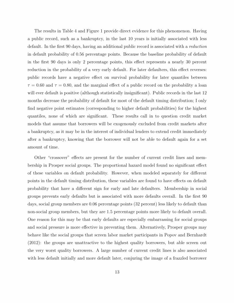
The results in Table 4 and Figure 1 provide direct evidence for this phenomenon. Having

a public record, such as a bankruptcy, in the last 10 years is initially associated with less

default. In the first 90 days, having an additional public record is associated with a reduction

in default probability of 0.56 percentage points. Because the baseline probability of default

in the first 90 days is only 2 percentage points, this effect represents a nearly 30 percent

reduction in the probability of a very early default. For later defaulters, this effect reverses:

public records have a negative effect on survival probability for later quantiles between

τ = 0.60 and τ = 0.80, and the marginal effect of a public record on the probability a loan

will ever default is positive (although statistically insignificant). Public records in the last 12

months decrease the probability of default for most of the default timing distribution; I only

find negative point estimates (corresponding to higher default probabilities) for the highest

quantiles, none of which are significant. These results call in to question credit market

models that assume that borrowers will be exogenously excluded from credit markets after

a bankruptcy, as it may be in the interest of individual lenders to extend credit immediately

after a bankruptcy, knowing that the borrower will not be able to default again for a set

amount of time.

Other “crossover” effects are present for the number of current credit lines and mem-

bership in Prosper social groups. The proportional hazard model found no significant effect

of these variables on default probability. However, when modeled separately for different

points in the default timing distribution, these variables are found to have effects on default

probability that have a different sign for early and late defaulters. Membership in social

groups prevents early defaults but is associated with more defaults overall. In the first 90

days, social group members are 0.06 percentage points (32 percent) less likely to default than

non-social group members, but they are 1.5 percentage points more likely to default overall.

One reason for this may be that early defaults are especially embarrassing for social groups

and social pressure is more effective in preventing them. Alternatively, Prosper groups may

behave like the social groups that screen labor market participants in Popov and Bernhardt

(2012): the groups are unattractive to the highest quality borrowers, but able screen out

the very worst quality borrowers. A large number of current credit lines is also associated

with less default initially and more default later, conjuring the image of a frazzled borrower

13

paying credit card bills off with other credit cards – the strategy works for a while, but

eventually the debt becomes overwhelming.

Finally, the effect of some borrower characteristics does not appear to change substantially

over the life of the loan. For example, more credit delinquencies has a strong and negative

effect on the probability of repayment at every point in the default timing distribution.

5 Empirical Implications

5.1 Example: Secondary Market for Loans

In this section, I use an example of loan resales to illustrate how the difference between the

proportional hazard model and the censored quantile regression model matter in practice.

Since the mid-1990s, the secondary market for loans has grown considerably in the United

States (Santos and Nigro (2007)), requiring third parties to assess the default risk of loans

long after the original transaction occurred. Prosper.com launched a secondary market for

Prosper loans in 2010. Although the Prosper secondary market updates information on the

borrower’s credit score range, all other financial variables are fixed at the level observed at

the time that the loan was first requested. I compare the predicted default rates derived

from the proportional hazard and quantile regression models for loans in their third year,

mirroring the risk evaluation that a trader in the secondary market for loans must perform.

I consider an example loan for $10,000 to the average low-, medium-, and high-risk

borrower, as defined by their credit score. Low-risk borrowers are defined as borrowers with

credit scores over 760, medium borrowers have credit scores in the range 640 to 679, and

high-risk borrowers fall in to the credit score range of 520 to 559. I choose the interest rate

as the average interest rate within these groups for loans between $9500 and $10500.9 Other

borrower characteristics are evaluated at the mean of each risk group. Table 5 presents the

covariate values for the example loans.

9I allow for a small range in amount of the loan when assessing the average interest rate because relatively

few loans in each group are for exactly $10,000.

14

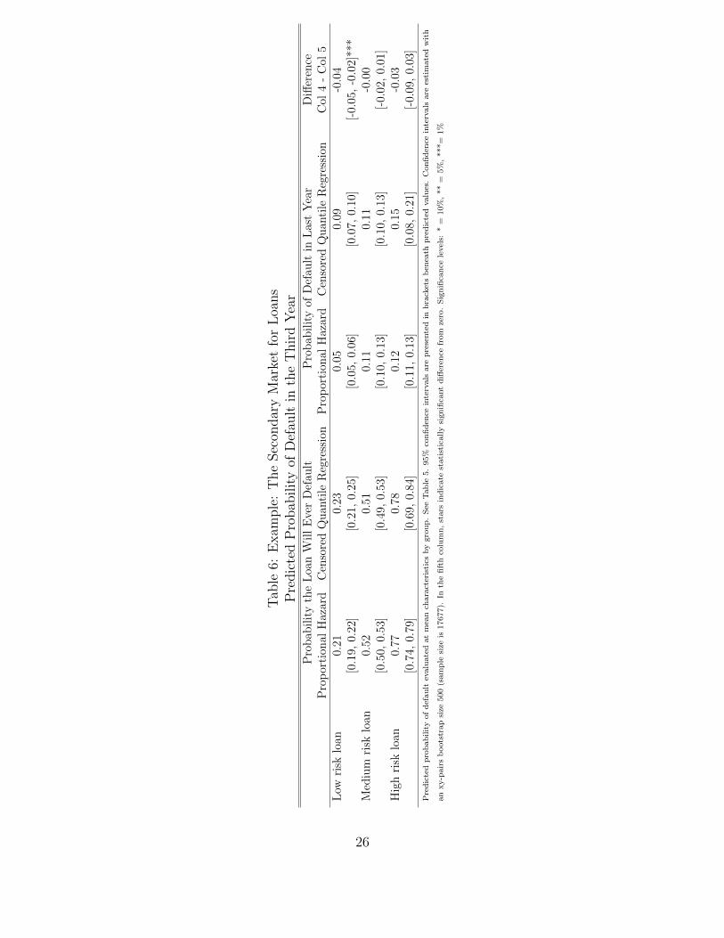
Table 6 shows predicted default probabilities derived from the proportional hazard and

censored quantile regression models estimated in Sections 3 and 4. Columns 2 and 3 display

the predicted probability from each model that the loan will default at some point during

the 3 year repayment period. Both the proportional hazard and quantile regression models

estimate remarkably similar probabilities of the loan ever defaulting. However, Columns 4

and 5 indicate that the quantile regression model finds different expected probabilities of

default in the last year. The expected probability of defaulting in the last year for a low-risk

loan is almost 70% higher when using estimates from the quantile regression model. This

difference is significant at the 0.01 level. Because the quantile regression model takes into

account the change in the effect of certain characteristics over time (see Figure 1), it results

in different predictions for the timing of loan default in ways that have practical implications

for loans resold on the secondary market.

5.2 Example: Expected Profit

Loans that default early lose close to the entire principal, whereas loans that default near

the end of their term may still generate a positive profit. Because default timing is crucial to

lender profitability, using a flexible approach such as quantile regression may be especially

useful in credit markets. In this section, I present an example of how expected profit of a

loan differs between the proportional hazard and the quantile regression model.

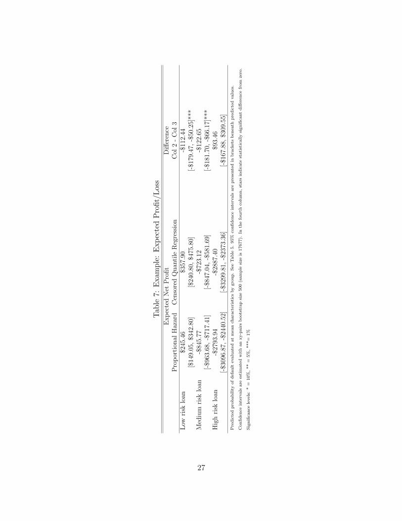
I use the predicted default probabilities at each month during the 36 month period from

the censored quantile regression model in Section 4 and the proportional hazard model in

Section 3 to estimate the expected profit of a loan for $10,000 made to a typical high-,

medium-, and low-risk borrower with the characteristics and interest rate described in Table

5. Table 7 reports expected profit, with 95% confidence intervals, for each loan. Although the

proportional hazard and the censored quantile regression estimate similar probabilities that

each loan will ever default (see Columns 1 and 2 of Table 6), the two models find significantly

different expected profit for the same loan because the effect of certain characteristics varies

significantly for early and late defaulters.

15

Because the quantile regression model predicts that defaults will occur later for high-

quality borrowers, the low- and medium-risk loans have significantly higher expected profit

when the predicted probabilities from the quantile regression model are used relative to

the proportional hazard model. Expected profit on low-risk loans is almost 45% higher

when predicted probabilities from the quantile regression are used. For medium-risk loans,

the quantile regression predicts an expected profit about 15% higher than the proportional

hazard model, although both models still predict a loss. The differences for both low- and

medium-risk loans are significant at the 0.01 level. Both the proportional hazard and the

quantile regression model predict equally abysmal losses for the high-risk loans.

6 Conclusion

This paper analyzes the default behavior of loans made on a peer-to-peer website using two

econometric methods: the widely-used proportional hazard model of Cox (1974) and the

more flexible censored quantile model described by Portnoy (2003) that allows the effects of

covariates to vary over the life of the loan. I find evidence that several traditional predictors

of default affect early and late defaulters differently, including “crossover” effects that cannot

be captured by a proportional hazard model. Incorporating this heterogeneity is especially

important in credit markets, where the timing of loan default substantially impacts recovery

rates and lender profitability.

I further illustrate the empirical implications of these differences with an example of

how the evaluation of a typical high-, medium-, and low-risk loan on the secondary market

changes when each model is used. While both models predict a similar probability that each

loan will ever default, the censored quantile regression model, because it takes into account

time-variation in the covariate effects, predicts a higher probability that low-risk loans will

default later. As a result, the expected profit for low- and medium-risk loans is substantially

higher when predicted default probabilities from the quantile regression are used rather than

the proportional hazard predicted probabilities. In this example, neglecting to account for

the time-varying effect of the covariates would lead to undervaluing low- and medium-risk

16

loans relative to high risk loans.

References

Adams, W., L. Einav, and J. Levin (2009). Liquidity constraints and imperfect information

in subprime lending. American Economic Review 99 (1), 49–84.

Agarwal, S., S. Chomsisengphet, and C. Liu (2011). Consumer bankruptcy and default: The

role of individual social capital. Journal of Economic Psychology 32, 632650.

Agarwal, S., S. Chomsisengphet, C. Liu, and N. S. Souleles (2009). Benefits of relation-

ship banking: Evidence from consumer credit markets. Federal Reserve Bank of Chicago

Working Paper Series.

Athreya, K. B. and H. P. Janicki (2009). Credit exclusion in quantitative models of

bankruptcy: Does it matter? Economic Quarterly 92 (1), 17–49.

Bellotti, T. and J. Crook (2007). Credit scoring with macroeconomic variables using survival

analysis. Working Paper. University of Edinburgh, Credit Research Centre.

Cai, J., J. Fan, H. Zhou, and Y. Zhou (2007). Hazard models with varying coefficients for

multivariate failure time data. The Annals of Statistics 35 (1), 324–354.

Ciochetti, B., R. Yao, and Y. Deng (2003). A proportional hazards model of commercial

loan mortgage default with originator bias. Journal of Real Estate Finance and Eco-

nomics 27 (1), 5–23.

Cohen-Cole, E., B. Duygan-Bump, and J. Montoriol-Garriga (2009). Forgive and forget:

Who gets credit after bankruptcy and why? Working Paper Series: Federal Reserve Bank

of Boston.

Cox, D. (1974). Regression models with life tables. Journal of the Royal Statistical Society 34,

187–220.

17

Duarte, J., S. Siegel, and L. Young (2009). Trust and credit. Working Paper, University of

Washington Business School.

Efron, B. (1967). The two-sample problem with censored data. Proc. Fifth Berkeley Sym-

posium in Mathematical Statistics 4.

Freedman, S. and G. Jin (2008). Do social networks solve information problems for peer-to-

peer lending? Evidence from Prosper.com. Working Paper, University of Maryland.

Glennon, D. and P. Nigro (2005). Measuring the default risk of small business loans: A

survival analysis approach. Journal of Money, Credit, and Banking 37 (5), 923–947.

Iyer, R., A. Khwaja, E. Luttmer, and K. Shue (2013). Screening peers softly: Inferring the

quality of small borrowers. NBER Working Paper No. 15242.

Koenker, R. and G. W. Bassett (1978). Regression quantiles. Econometrica 46 (1), 33–50.

Koenker, R. and Y. Bilias (2001). Quantile regression for duration data: A reappraisal of

the Pennsylvania re-employment bonus experiments. Empirical Economics 26, 199–200.

Koenker, R. and O. Geling (2001). Reappraising medfly longevity: A quantile regression

survival analysis. Journal of the American Statistical Association 96, 458–468.

Lin, M., N. Prabhala, and S. Viswanathan (2012). Judging borrowers by the company they

keep: Friendship networks and information asymmetry in online peer-to-peer lending.

forthcoming, Management Science.

Miller, S. (2012). Information and default in consumer credit markets: Evidence from a

natural experiment. Working Paper. University of Illinois Department of Economics.

Pennington-Cross, A. (2003). Credit history and the performance of prime and nonprime

mortgages. Journal of Real Estate Finance and Economics 27 (3), 279–301.

Pope, D. and J. Sydnor (2011). What’s in a picture? Evidence of discrimination from

Prosper.com. Journal of Human Resources 46 (1), 53–92.

18

Popov, S. and D. Bernhardt (2012). Fraternities and labor market outcomes. American

Economic Journal: Microeconomics 4 (1), 116–141.

Porter, K. (2008). Bankrupt profits: The credit industrys business model for postbankruptcy

lending. Iowa Law Review 93, 1369–1421.

Portnoy, S. (2003). Censored regression quantiles. Journal of the American Statistical As-

sociation 98 (464), 1001–1012.

Powell, J. (1986). Censored regression quantiles. Journal of Econometrics 32, 143–155.

Ramcharan, R. and C. Crowe (2013). The impact of house prices on consumer credit:

Evidence from an internet bank. Journal of Money, Credit, and Banking 45 (6), 10851115.

Ravina, E. (2012). Love and loans: The effect of beauty and personal characteristics in credit

markets. Working Paper, Columbia University Graduate School of Business.

Rigbi, O. (2011). The effects of usury laws: Evidence from the online loan market. forth-

coming, Review of Economics and Statistics.

Santos, J. A. and P. Nigro (2007). Is the secondary loan market valuable for borrowers?

Working Paper. Available at SSRN: http://ssrn.com/abstract=1026788.

Sun, Y., R. Sundaram, and Y. Zhao (2009). Empirical likelihood inference for the Cox

model with time-dependent coefficients via local partial likelihood. Scandinavian Journal

of Statistics 36 (3), 444–462.

Tian, L., D. Zucker, and L.-J. Wei (2005). On the Cox model with time-varying regression

coefficients. Journal of the American Statistical Association 100, 172–183.

19

Fig

ure

1:C

ondit

ional

Quan

tile

Eff

ects

onT

ime

toD

efau

lt

0.2

0.4

0.6

0.8

−0.040.000.04

Cre

ditS

core

oooooooooooooo

ooo

o

0.2

0.4

0.6

0.8

−4e−050e+004e−05

Cre

ditS

core

2

ooooooooooooooooo

o

0.2

0.4

0.6

0.8

−0.40.00.2G

roup

Dum

my

ooooooooooooooooo

o

0.2

0.4

0.6

0.8

−7e−05−4e−05

Am

ount

oooooooooooo

oo

oooo

0.2

0.4

0.6

0.8

−0.4−0.20.0

Bor

row

erR

ate

ooooooooooooo

o

ooo

o

0.2

0.4

0.6

0.8

−0.0040.0020.006

Bor

row

erR

ate2

oooooooooooooo

ooo

o

0.2

0.4

0.6

0.8

−0.100.00

Deb

tToI

ncom

eRat

io

o

ooooooo

oooooo

ooo

o

0.2

0.4

0.6

0.8

−0.6−0.2

Hom

e

oooooooooooooo

o

o

o

o

0.2

0.4

0.6

0.8

−0.08−0.040.00

Cur

rent

Del

inqu

enci

es

ooooooooooooooo

ooo

0.2

0.4

0.6

0.8

0.000.020.04

Del

inqu

enci

esLa

st7Y

ears

oooooooooooooooo

o

o

0.2

0.4

0.6

0.8

−0.08−0.05−0.02

Inqu

iries

Last

6Mon

ths

oooooooooooo

oooo

o

o

0.2

0.4

0.6

0.8

−0.100.00Publ

icR

ecor

dsLa

st10

Year

s

o

oooo

ooooooooooooo

0.2

0.4

0.6

0.8

−0.3−0.10.10.3Publ

icR

ecor

dsLa

st12

Mon

ths

ooooooooooo

ooo

oo

oo

0.2

0.4

0.6

0.8

0.000.050.10

Ope

nCre

ditL

ines

oooooooooooooooo

o

o

0.2

0.4

0.6

0.8

−0.20.00.20.4

City

Dum

my

oooooooooooooooo

o

o

0.2

0.4

0.6

0.8

−0.20.00.20.4

Fullt

ime

oooooooooooooooooo

0.2

0.4

0.6

0.8

−0.40.00.4

Ban

kcar

dUtil

izat

ion

oooooooooooooooo

o

o

0.2

0.4

0.6

0.8

−5.0e−061.0e−05

Rev

olvi

ngC

redi

tBal

ance

ooooooooooooooooo

o

0.2

0.4

0.6

0.8

−1e−051e−05

Am

ount

Del

inqu

ent

oooooooooooooo

oooo

0.2

0.4

0.6

0.8

−0.0100.0000.010

Tota

lCre

ditL

ines

ooooooooooooo

o

ooo

o

0.2

0.4

0.6

0.8

−0.100.00

Cur

rent

Cre

ditL

ines

oooooooooooooooo

oo

0.2

0.4

0.6

0.8

−5515

Inte

rcep

t

oooooooooooooo

ooo

o

20

Tab

le1:

Des

crip

tive

Sta

tist

ics

Var

iable

Nam

eD

escr

ipti

onM

ean

Min

/Max

Am

ount

Dol

lar

amou

nt

oflo

an65

8310

00/2

5000

Bor

row

erR

ate

Inte

rest

rate

pai

dby

bor

row

er17.9

80.

01/3

6.00

Cit

yD

um

my

Bin

ary

vari

able

takin

ga

valu

eof

1if

the

bor

row

eris

are

siden

tof

aci

ty0.

140/

1C

urr

ent

Del

inquen

cies

Num

ber

ofcr

edit

lines

curr

entl

ylist

edas

del

inquen

t1.

030/

83D

ebt

toIn

com

eR

atio

Rat

ioof

dol

lar

valu

eof

outs

tandin

gdeb

tto

self

-rep

orte

din

com

e0.

340/

10D

elin

quen

cies

Las

t7

Yea

rsN

um

ber

ofdel

inquen

tac

counts

inth

ela

stse

ven

year

s5.

100/

99F

ullti

me

Bin

ary

vari

able

takin

ga

valu

eof

1if

the

bor

row

erre

por

tsth

eyar

e0.

880/

1em

plo

yed

full-t

ime

Gro

up

Dum

my

Bin

ary

vari

able

takin

ga

valu

eof

1if

the

bor

row

eris

am

emb

erof

0.31

0/1

aP

rosp

erso

cial

grou

pH

ome

Bin

ary

vari

able

takin

ga

valu

eof

1if

the

bor

row

eris

ahom

eow

ner

0.47

0/1

Inquir

ies

Las

t6

Mon

ths

Num

ber

ofti

mes

the

cred

itre

por

thas

bee

nre

ques

ted

2.63

0/63

Public

Rec

ords

Las

t10

Yea

rsN

um

ber

ofpublic

reco

rds,

such

asban

kru

ptc

ies

orlien

s,list

edon

0.38

0/30

the

bor

row

er’s

cred

itre

por

tin

the

last

10ye

ars

Public

Rec

ords

Las

t12

Mon

ths

Num

ber

ofpublic

reco

rds,

such

asban

kru

ptc

ies

orlien

s,list

edon

0.04

0/7

the

bor

row

er’s

cred

itre

por

tin

the

last

year

Op

enC

redit

Lin

esN

um

ber

ofac

tive

lines

ofcr

edit

inth

eb

orro

wer

’snam

e8.

210/

45C

urr

ent

Cre

dit

Lin

esN

um

ber

ofop

enor

clos

edac

counts

inth

eb

orro

wer

’snam

eth

atth

e9.

412/

129

bor

row

eris

pay

ing

onti

me

Tot

alC

redit

Lin

esT

otal

num

ber

ofcr

edit

lines

list

edin

the

bor

row

er’s

cred

itre

por

t24.3

52/

129

Am

ount

Del

inquen

tD

olla

rva

lue

ofto

tal

del

inquen

cies

1163

0/44

4745

Ban

kcar

dU

tiliza

tion

Ban

kcar

ddeb

tdiv

ided

by

avai

lable

cred

it0.

550/

5.95

Rev

olvin

gC

redit

Bal

ance

Outs

tandin

gbal

ance

oncr

edit

card

sor

other

revo

lvin

gcr

edit

acco

unts

1135

20/

9999

4Sam

ple

Siz

e:17

677

Sam

ple

incl

ud

esall

loan

sm

ad

eby

firs

t-ti

me

borr

ow

ers

issu

edth

rou

gh

Pro

sper

bet

wee

nF

ebru

ary

17,

2007

an

dN

ovem

ber

30,

2009.

Pro

sper

data

an

dE

xp

eria

ncr

edit

score

ran

ges

dow

nlo

ad

edby

the

au

thor

from

Pro

sper

.com

on

02/11/2011.

21

Table 2: Credit Grade-Category Mapping

Experian Scorex PLUS Credit Range Credit Grade Credit Score Assigned Percent of Sample880− 899 AA 889.5 0.04860− 879 AA 869.5 0.03840− 859 AA 849.5 0.59820− 839 AA 829.5 1.31800− 819 AA 809.5 1.96780− 799 AA 789.5 3.51760− 779 AA 769.5 5.17740− 759 A 749.5 5.37720− 739 A 729.5 7.16700− 719 B 709.5 7.03680− 699 B 689.5 9.32660− 679 C 669.5 8.59640− 659 C 649.5 12.84620− 639 D 629.5 9.70600− 619 D 609.5 9.29580− 599 E 589.5 3.91560− 579 E 569.5 4.77540− 559 HR 549.5 3.47520− 539 HR 529.5 5.62

Sample includes all loans made by first-time borrowers issued through Prosper between February 17, 2007 and November 30, 2009

Prosper data and Experian credit score ranges downloaded by the author from Prosper.com on 02/11/2011.

22

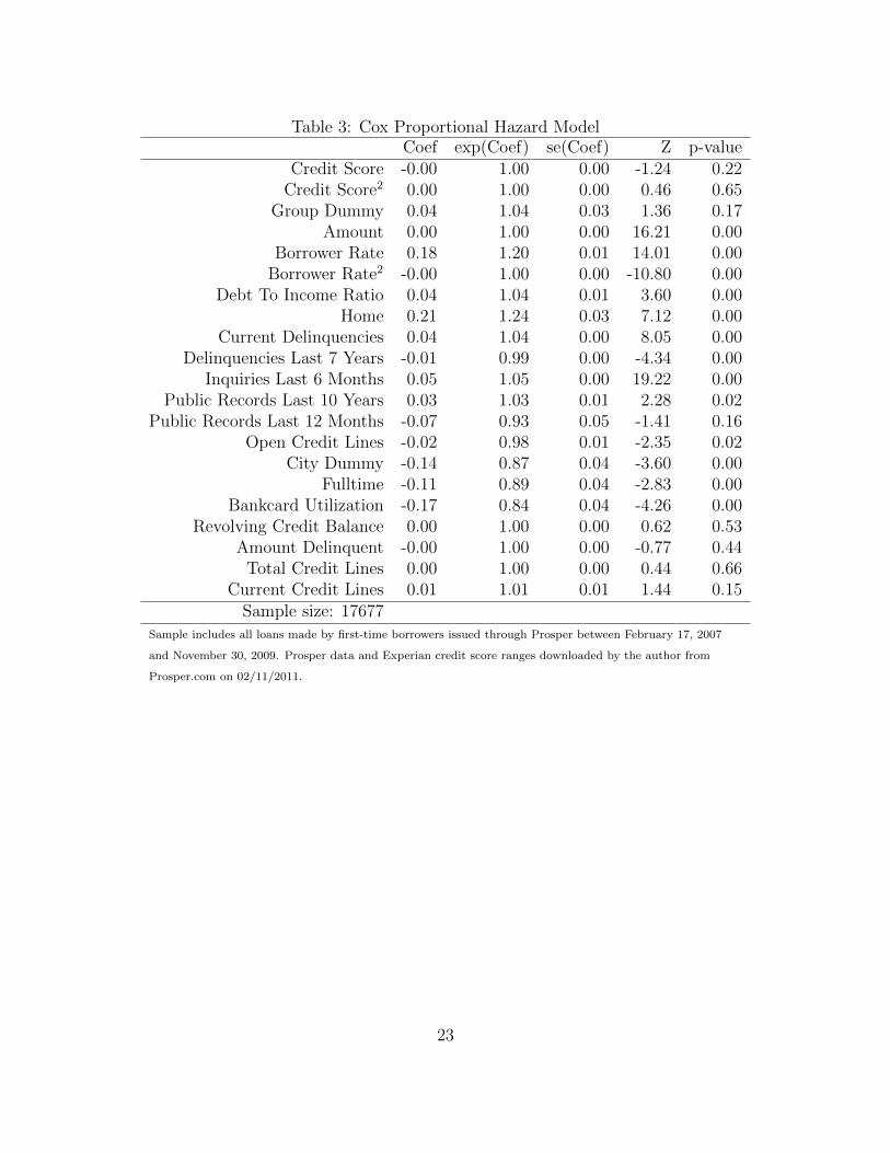
Table 3: Cox Proportional Hazard ModelCoef exp(Coef) se(Coef) Z p-value

Credit Score -0.00 1.00 0.00 -1.24 0.22Credit Score2 0.00 1.00 0.00 0.46 0.65

Group Dummy 0.04 1.04 0.03 1.36 0.17Amount 0.00 1.00 0.00 16.21 0.00

Borrower Rate 0.18 1.20 0.01 14.01 0.00Borrower Rate2 -0.00 1.00 0.00 -10.80 0.00

Debt To Income Ratio 0.04 1.04 0.01 3.60 0.00Home 0.21 1.24 0.03 7.12 0.00

Current Delinquencies 0.04 1.04 0.00 8.05 0.00Delinquencies Last 7 Years -0.01 0.99 0.00 -4.34 0.00

Inquiries Last 6 Months 0.05 1.05 0.00 19.22 0.00Public Records Last 10 Years 0.03 1.03 0.01 2.28 0.02

Public Records Last 12 Months -0.07 0.93 0.05 -1.41 0.16Open Credit Lines -0.02 0.98 0.01 -2.35 0.02

City Dummy -0.14 0.87 0.04 -3.60 0.00Fulltime -0.11 0.89 0.04 -2.83 0.00

Bankcard Utilization -0.17 0.84 0.04 -4.26 0.00Revolving Credit Balance 0.00 1.00 0.00 0.62 0.53

Amount Delinquent -0.00 1.00 0.00 -0.77 0.44Total Credit Lines 0.00 1.00 0.00 0.44 0.66

Current Credit Lines 0.01 1.01 0.01 1.44 0.15Sample size: 17677

Sample includes all loans made by first-time borrowers issued through Prosper between February 17, 2007

and November 30, 2009. Prosper data and Experian credit score ranges downloaded by the author from

Prosper.com on 02/11/2011.

23

Table 4: Estimated Marginal Effects of Borrower Characteristics in Default Probabilities byTime, Censored Quantile Regression Model

Effect on default: First 90 Days First Year EverCredit Score -0.0002 -0.0003 -0.0004

[-0.0003, 0.0001] [-0.0005, -0.0002]*** [-0.0005,-0.0002]***Group Dummy -0.006 -0.011 0.0152

[-0.0133, 0.0002]* [-0.0188,-0.0019]** [0.0012,0.0292]**Debt To Income Ratio -0.0016 0.0053 0.0059

[-0.0014, 0.0046] [0.0007,0.0094]** [0.0025, 0.0129]**Home -0.0027 0.0196 0.0477

[-0.0100, 0.0037] [0.0113, 0.0306]*** [0.0340, 0.0628]***Current Delinquencies 0.0026 0.0064 0.0102

[-0.0018, 0.0041]* [0.0041,0.0094]*** [0.0074, 0.015]***Delinquencies Last 7 Years 0.0004 -0.0007 -0.0016

[-0.0009, 0.0090] [-0.0013,-0.0001]** [-0.0024, -0.0005]**Inquiries Last 6 Months 0.0016 0.0059 0.0116

[-0.0019, 0.0034] [0.0044, 0.0077]*** [0.0096, 0.0149]***Public Records Last 10 Years -0.0056 -0.0019 0.0018

[-0.0050, 0.0006]* [-0.0040, 0.0041] [-0.0015, 0.0119]Public Records Last 12 Months -0.0030 -0.0118 -0.0199

[-0.0075, 0.0108] [-0.0224, 0.0029] [-0.0462, 0.0022]City Dummy -0.0051 -0.0192 -0.0374

[-0.0106, 0.0051] [-0.0270, -0.0085]*** [-0.0518, -0.0232]***Fulltime -0.0001 -0.0212 -0.0376

[-0.0093, 0.0074] [-0.0324, -0.0097]*** [-0.0567,-0.0181]***Bankcard Utilization -0.0112 -0.0315 -0.0425

[-0.0164, -0.0011]** [-0.0423, -0.0212]** [-0.0640,-0.0022]***Revolving Credit Balance 0.0010 0.0003 0.00002

[-0.0012, 0.0007] [-0.0001, 0.0006] [-0.0002, 0.0012]Amount Delinquent -0.0031 -0.0002 -0.0029

[-0.0010, 0.0013] [-0.0010, 0.0009] [-0.0023, 0.0004]Open Credit Lines -0.0003 -0.0022 -0.0082

[-0.0059, 0.0075] [-0.0089, 0.0046] [-0.0189, 0.0013]Total Credit Lines -0.0038 0.0002 -0.0019

[-0.0021, 0.0014] [-0.0009, 0.0017] [-0.0009, 0.0042]Current Credit Lines -0.0047 -0.0030 0.0020

[-0.0100,0.0031] [-0.0094, 0.0043] [-0.0089, 0.0117]Baseline probability of default (τ): 0.019 0.116 0.318Sample size: 17677This table displays the marginal effects of Credit Score (increase of 1 point), Current Delinquencies (increase of 1), Revolving Credit

Balance (increase of $1000), Amount Delinquent (increase of $1000), Debt to Income Ratio (increase of 1), Total, Open, and Current Credit

Lines (increase of 3 lines), Bankcard Utilization (increase of 1). Binary variables show the effect of moving from 0 to 1. Marginal

effects computed at the sample median. Sample includes all loans made to first-time borrowers issued through Prosper between February

17, 2007 and November 30, 2009. Prosper data and Experian credit score ranges downloaded by the author from Prosper.com on 02/11/2011.

24

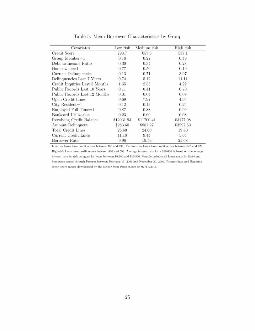
Table 5: Mean Borrower Characteristics by Group

Covariates Low risk Medium risk High riskCredit Score 793.7 657.5 537.1Group Member=1 0.18 0.27 0.49Debt to Income Ratio 0.30 0.34 0.28Homeowner=1 0.77 0.50 0.19Current Delinquencies 0.13 0.71 3.97Delinquencies Last 7 Years 0.74 5.12 11.11Credit Inquiries Last 5 Months 1.65 2.53 4.22Public Records Last 10 Years 0.11 0.41 0.70Public Records Last 12 Months 0.01 0.04 0.09Open Credit Lines 9.69 7.97 4.95City Resident=1 0.12 0.13 0.24Employed Full Time=1 0.87 0.88 0.90Bankcard Utilization 0.23 0.60 0.68Revolving Credit Balance $12931.93 $11700.41 $3177.98Amount Delinquent $283.60 $881.27 $3297.50Total Credit Lines 26.60 24.60 19.40Current Credit Lines 11.18 9.44 5.64Borrower Rate 9.96 19.53 25.68Low-risk loans have credit scores between 760 and 899. Medium-risk loans have credit scores between 640 and 679.

High-risk loans have credit scores between 520 and 559. Average interest rate for a $10,000 is based on the average

interest rate by risk category for loans between $9,500 and $10,500. Sample includes all loans made by first-time

borrowers issued through Prosper between February 17, 2007 and November 30, 2009. Prosper data and Experian

credit score ranges downloaded by the author from Prosper.com on 02/11/2011.

25

Tab

le6:

Exam

ple

:T

he

Sec

ondar

yM

arke

tfo

rL

oans

Pre

dic

ted

Pro

bab

ilit

yof

Def

ault

inth

eT

hir

dY

ear

Pro

bab

ilit

yth

eL

oan

Wil

lE

ver

Def

ault

Pro

bab

ilit

yof

Def

ault

inL

ast

Yea

rD

iffer

ence

Pro

por

tion

alH

azar

dC

enso

red

Quan

tile

Reg

ress

ion

Pro

por

tion

alH

azar

dC

enso

red

Qu

anti

leR

egre

ssio

nC

ol4

-C

ol5

Low

risk

loan

0.21

0.23

0.05

0.09

-0.0

4[0

.19,

0.22

][0

.21,

0.25

][0

.05,

0.06

][0

.07,

0.10

][-

0.05

,-0

.02]

***

Med

ium

risk

loan

0.52

0.51

0.11

0.11

-0.0

0[0

.50,

0.53

][0

.49,

0.53

][0

.10,

0.13

][0

.10,

0.13

][-

0.02

,0.

01]

Hig

hri

sklo

an0.

770.

780.

120.

15-0

.03

[0.7

4,0.

79]

[0.6

9,0.

84]

[0.1

1,0.

13]

[0.0

8,0.

21]

[-0.

09,

0.03

]P

red

icte

dp

rob

ab

ilit

yof

def

au

ltev

alu

ate

dat

mea

nch

ara

cter

isti

csby

gro

up

.S

eeT

ab

le5.

95%

con

fid

ence

inte

rvals

are

pre

sente

din

bra

cket

sb

enea

thp

red

icte

dvalu

es.

Con

fid

ence

inte

rvals

are

esti

mate

dw

ith

an

xy-p

air

sb

oots

trap

size

500

(sam

ple

size

is17677).

Inth

efi

fth

colu

mn

,st

ars

ind

icate

stati

stic

all

ysi

gn

ifica

nt

diff

eren

cefr

om

zero

.S

ign

ifica

nce

level

s:*

=10%

,**

=5%

,***=

1%

26

Tab

le7:

Exam

ple

:E

xp

ecte

dP

rofit/

Los

sE

xp

ecte

dN

etP

rofi

tD

iffer

ence

Pro

por

tion

alH

azar

dC

enso

red

Qu

anti

leR

egre

ssio

nC

ol2

-C

ol3

Low

risk

loan

$245

.46

$357

.90

-$11

2.44

[$14

9.05

,$3

42.8

0][$

240.

80,

$475

.80]

[-$1

79.4

7,-$

50.2

5]**

*M

ediu

mri

sklo

an-$

845.

77-$

723.

12-$

122.

65[-

$963

.68,

-$71

7.41

][-

$847

.04,

-$58

1.69

][-

$181

.70,

-$66

.17]

***

Hig

hri

sklo

an-$

2793

.94

-$28

87.4

0$9

3.46

[-$3

096.

87,

-$24

40.5

2][-

$329

9.81

,-$

2373

.36]

[-$1

67.8

8,$3

09.5

5]P

red

icte

dp

rob

ab

ilit

yof

def

au

ltev

alu

ate

dat

mea

nch

ara

cter

isti

csby

gro

up

.S

eeT

ab

le5.

95%

con

fid

ence

inte

rvals

are

pre

sente

din

bra

cket

sb

enea

thp

red

icte

dvalu

es.

Con

fid

ence

inte

rvals

are

esti

mate

dw

ith

an

xy-p

air

sb

oots

trap

size

500

(sam

ple

size

is17677).

Inth

efo

urt

hco

lum

n,

stars

ind

icate

stati

stic

all

ysi

gn

ifica

nt

diff

eren

cefr

om

zero

.

Sig

nifi

can

cele

vel

s:*

=10%

,**

=5%

,***=

1%

27