Risk consideration in electricity generation unit

commitment under supply and demand uncertainty

by

Narges Kazemzadeh

A dissertation submitted to the graduate faculty

in partial fulfillment of the requirements for the degree of

DOCTOR OF PHILOSOPHY

Major: Industrial Engineering

Sarah M. Ryan, Major Professor

Jing Dong

Sigurdur Olafsson

Jo Min

Lizhi Wang

Iowa State University

Ames, Iowa

2016

ii

To my husband,

Mahdi,

And to our daughter,

Nika.

iii

TABLE OF CONTENTS

ACKNOWLEDGEMENTS vii

ABSTRACT viii

1. OVERVIEW 1

1.1 Introduction . . . . . . . . . . . . . . . . . . . . . . . . . . . . . . 1

1.2 Problem Statement . . . . . . . . . . . . . . . . . . . . . . . . . . 2

1.3 Organization of the Dissertation . . . . . . . . . . . . . . . . . . 3

2. ROBUST OPTIMIZATION VS. STOCHASTIC PROGRAM-

MING CONSIDERING RISK FOR UNIT COMMITMENT

WITH UNCERTAIN VARIABLE RENEWABLE GENER-

ATION 6

2.1 Introduction . . . . . . . . . . . . . . . . . . . . . . . . . . . . . . 6

2.2 Mathematical Models . . . . . . . . . . . . . . . . . . . . . . . . 10

2.2.1 Sets, Parameters, and Decision Variables . . . . . . . . . 10

2.2.2 Constraints . . . . . . . . . . . . . . . . . . . . . . . . . . 13

2.2.3 Stochastic Programming Unit Commitment Model In-

cluding CVaR (SUC-CVaR) . . . . . . . . . . . . . . . . . 16

2.2.4 Robust Unit Commitment Model (RUC) . . . . . . . . . . 18

2.3 Scenarios vs. Uncertainty Sets . . . . . . . . . . . . . . . . . . . 19

2.4 Numerical Experiments . . . . . . . . . . . . . . . . . . . . . . . 22

2.4.1 Implementation details . . . . . . . . . . . . . . . . . . . . 23

2.4.2 Results . . . . . . . . . . . . . . . . . . . . . . . . . . . . 24

2.5 Conclusions . . . . . . . . . . . . . . . . . . . . . . . . . . . . . . 32

iv

3. IMPROVING SOLUTION METHODS FOR ROBUST UNIT

COMMITMENT 33

3.1 Introduction . . . . . . . . . . . . . . . . . . . . . . . . . . . . . . 33

3.2 The Existing Method . . . . . . . . . . . . . . . . . . . . . . . . . 35

3.2.1 Outer approximation to evaluate R(y1) . . . . . . . . . . 37

3.2.2 Cutting plane method to solve the master problem . . . . 40

3.3 Branch-and-Cut Method for Solving the Robust Optimization

Problem . . . . . . . . . . . . . . . . . . . . . . . . . . . . . . . . 41

3.4 Details of the Formulation . . . . . . . . . . . . . . . . . . . . . . 46

3.5 Computational Results . . . . . . . . . . . . . . . . . . . . . . . . 49

3.6 Conclusions . . . . . . . . . . . . . . . . . . . . . . . . . . . . . . 51

4. AN APPROXIMATION FOR CVAR OF ELECTRIC POWER

PRODUCTION COST CONSIDERING GENERATING UNIT

FAILURES 52

4.1 Introduction . . . . . . . . . . . . . . . . . . . . . . . . . . . . . . 52

4.2 Problem Statement . . . . . . . . . . . . . . . . . . . . . . . . . . 56

4.3 Numerical Experiment . . . . . . . . . . . . . . . . . . . . . . . . 60

4.4 Conclusions . . . . . . . . . . . . . . . . . . . . . . . . . . . . . . 66

5. GENERAL CONCLUSION 68

6. BIBLIOGRAPHY 71

v

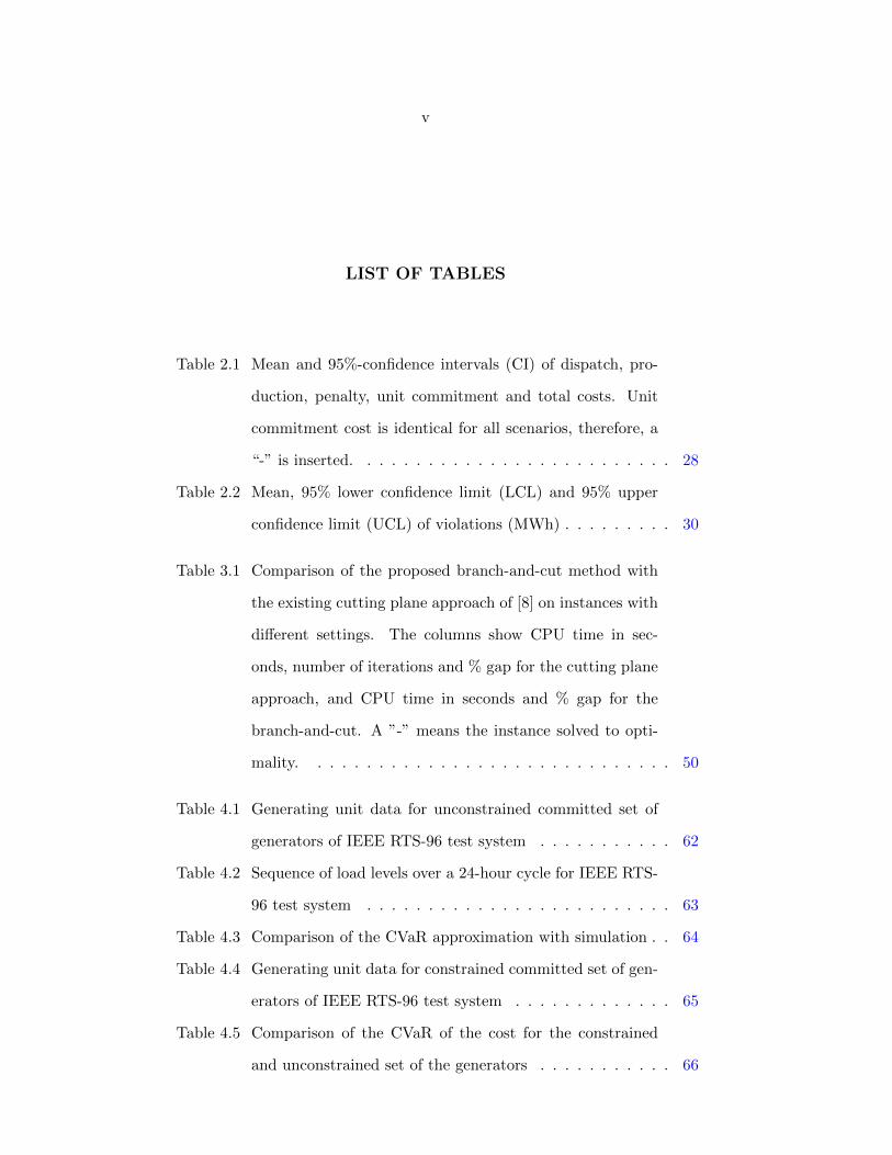
LIST OF TABLES

Table 2.1 Mean and 95%-confidence intervals (CI) of dispatch, pro-

duction, penalty, unit commitment and total costs. Unit

commitment cost is identical for all scenarios, therefore, a

“-” is inserted. . . . . . . . . . . . . . . . . . . . . . . . . . 28

Table 2.2 Mean, 95% lower confidence limit (LCL) and 95% upper

confidence limit (UCL) of violations (MWh) . . . . . . . . . 30

Table 3.1 Comparison of the proposed branch-and-cut method with

the existing cutting plane approach of [8] on instances with

different settings. The columns show CPU time in sec-

onds, number of iterations and % gap for the cutting plane

approach, and CPU time in seconds and % gap for the

branch-and-cut. A ”-” means the instance solved to opti-

mality. . . . . . . . . . . . . . . . . . . . . . . . . . . . . . 50

Table 4.1 Generating unit data for unconstrained committed set of

generators of IEEE RTS-96 test system . . . . . . . . . . . 62

Table 4.2 Sequence of load levels over a 24-hour cycle for IEEE RTS-

96 test system . . . . . . . . . . . . . . . . . . . . . . . . . 63

Table 4.3 Comparison of the CVaR approximation with simulation . . 64

Table 4.4 Generating unit data for constrained committed set of gen-

erators of IEEE RTS-96 test system . . . . . . . . . . . . . 65

Table 4.5 Comparison of the CVaR of the cost for the constrained

and unconstrained set of the generators . . . . . . . . . . . 66

vi

LIST OF FIGURES

2.1 Stepwise startup cost . . . . . . . . . . . . . . . . . . . . . . . . 14

2.2 Modified IEEE-RTS-96 . . . . . . . . . . . . . . . . . . . . . . . 23

2.3 Probabilistic scenarios and worst cases in each uncertainty set . 24

2.4 Distributions of unit commitment cost plus production cost . . . 25

2.5 Distributions of total cost . . . . . . . . . . . . . . . . . . . . . . 26

2.6 Pareto chart of expected shortage vs. unit commitment cost plus

expected production cost. . . . . . . . . . . . . . . . . . . . . . . 26

2.7 Pareto chart of penalty cost vs. unit commitment cost from

dispatching unit commitment schedules found by different for-

mulations and settings in the worst case of U2(α = 0.1) . . . . . 29

2.8 Comparison of different penalties for SUC-CVaR (γ = 0.05),

RUC-U1 (∆ = 0.2|Nd|) and RUC-U2 (α = 0.5) . . . . . . . . . . 31

vii

ACKNOWLEDGEMENTS

First and foremost, I would like to take this opportunity to express the

deepest thanks to my major professor, Dr. Sarah M. Ryan for her guidance,

patience, continuous support of my research and allowing me flexibility to ex-

plore ideas that were interesting to me.

I would additionally like to thank my committee members, Dr. Jing Dong,

Dr, Jo Min, Dr. Sigurdur Olafsson and Dr. Lizhi Wang for their helpful

guidance and feedback.

I also extend my utmost gratitude to my family. Thanks to my parents for

encouraging me to pursue graduate education and being my biggest source of

inspiration. I cannot thank them enough for supporting me throughout my life.

Thanks to my husband, Mahdi, for his continued love, patience and support

throughout the graduate school experience, and our daughter, Nika, for all of

the joys she has provided since she entered this world.

Finally, I thank God for letting me through all the difficulties. You are the

one who provide me with the strength to finish my degree.

viii

ABSTRACT

Unit commitment (UC) seeks the most cost effective generator commitment

schedule for an electric power system to meet net load while satisfying the

operational constraints on transmission system and generation resources. This

problem is challenging because of the high level of uncertainty in net load which

results from load uncertainty and renewable generation uncertainty. This dis-

sertation addresses topics in modeling and computational aspects of considering

risk in UC problems.

We investigate and compare the performance of stochastic programming and

robust optimization as the most widely studied approaches for unit commitment

under net load uncertainty. We explicitly account for risk, via conditional value

at risk (CVaR), in the stochastic programming objective function and by em-

ploying a CVaR-based uncertainty set in the robust optimization formulation.

The numerical results indicate that the stochastic program with CVaR evalu-

ated in a low probability tail is able to achieve better cost-risk trade-offs than

the robust formulation. The CVaR-based uncertainty set similarly outperforms

an uncertainty set based only on ranges.

Being able to solve UC problem in short amount of time on a daily ba-

sis is one of the challenges power system operators face. Therefore, we also

adopt a branch-and-cut approach to improve the solution algorithm for robust

optimization formulation of the UC problem.

Finally, we present an asymptotic approximation for the CVaR of cost in

a power system accounting for generating unit outages. This approximation

provides a fast computation of the risk emanating from a set of committed

generators due to their imperfect reliability.

1

CHAPTER 1. OVERVIEW

1.1 Introduction

In recent years, with an ongoing increase in power generation, the power

industry plays an important role in modern society. Therefore, a significant

amount of attention has been paid to developing a secure, reliable and economic

power supply. Unit commitment (UC) is one of the important tasks in electrical

power system operations. It is an optimization problem, concerned with slow-

responding thermal generating units, to determine the operation schedule of

these generating units to meet forecast net load at minimum cost under different

constraints and environments. However, there are challenges appearing in the

UC problem due to the high level of uncertainty associated with supply and

demand of electricity power. In this study, we investigate approaches to address

the consideration of risk associated with these sources of uncertainty in the UC

problem.

Because of global warming and other environmental issues caused by fossil

fuels, there is an increasing interest in using renewable energy resources such

as wind or solar. The United States targets to supply 20% of its electricity

generation capacity using wind energy by 2030 [1]. Although several regions

of the US and world (including Iowa) already well exceed this goal, the most

critical challenges to meeting this goal come from increases in variability and

uncertainty in net load. Net load is defined as the difference between the load

and the output of renewable generation. Uncertainty in net load results from

both load uncertainty and renewable generation uncertainty. Another source of

2

uncertainty associated with UC includes unexpected generator and transmission

line outages which may cause difficulties for the scheduled generators to meet

the net load.

This dissertation addresses several topics in modeling and computational

aspects of considering risk in UC problems.

1.2 Problem Statement

Unit commitment, as an important task in electric power system operations,

seeks the most cost-effective generator commitment decisions of the system to

meet load while satisfying operational constraints on the transmission system

and generation resources. This problem is challenging because of the high level

of uncertainty in net load which results from load uncertainty and renewable

generation uncertainty.

One of the potential solutions to deal with the uncertainty in UC is to in-

crease fixed operating reserves [41]. Reserve is a level of generation resources

which is scheduled to respond to generation shortages and prevent load dis-

connection. Imposing reserve constraints on the UC problem, however, incurs

extra operational cost, and does not explicitly model the uncertainty. In con-

trast, one can employ techniques for optimization under uncertainty. Stochastic

unit commitment (SUC) and robust unit commitment (RUC) have been intro-

duced as promising tools to deal with the uncertainty associated with net load

forecast. The idea of SUC is to utilize a scenario-based uncertainty represen-

tation in the UC formulation. Compared to simply using reserve constraints,

stochastic optimization models have certain advantages, such as cost savings

and reliability improvement [54, 53]. In contrast to stochastic programming

models, RUC models incorporate uncertainty only in terms of the ranges of

the uncertain quantities, regardless of the information concerning their under-

lying probability distributions. Instead of minimizing the total expected cost

as seen usually in SUC, RUC minimizes the worst case cost regarding all pos-

3

sible outcomes of the uncertain parameters within these specified ranges. This

type of model certainly produces more conservative solutions; however, it can

avoid incorporating a large number of scenarios. Another possibility is to utilize

conditional value at risk (CVaR) or other risk measures in combination with

these methods. CVaR is a risk measure popular for its coherency properties

and computational advantages. Considering the probability density function of

loss and γ as a parameter indicating the right tail probability of that function,

CVaRγ is defined as the expected value in the worst 100γ% of loss [51].

Other uncertainties associated with UC problem include unexpected genera-

tor and transmission line outages. Unexpected outages of power grid elements,

such as transmission lines and generators, can result in dramatic electricity

shortages. Since reliability is important in power grid operations, handling

these unexpected outages has become an interesting research area in recent

years.

1.3 Organization of the Dissertation

The dissertation is organized in a three-paper format, but all the references

are combined at the end. It addresses topics of risk consideration in the unit

commitment problem under supply and demand uncertainty. These topics in-

clude various approaches to considering risk in the unit commitment problem

and methodologies to solve the resulting optimization or estimation problems.

In Chapter 2, we study the unit commitment problem with two commonly

used approaches; stochastic programming and robust optimization. Our stochas-

tic programming formulation minimizes the start-up and shut-down cost as well

as the CVaR of production cost and penalty cost. In the literature, stochastic

programs often optimize expected value of cost in the objective function. In

contrast, we utilize a risk measure in the objective function to address the risk

associated with the cost. One of the challenges in the robust optimization ap-

proach is constructing a proper uncertainty set. We consider two approaches to

4

develop the uncertainty sets. The first approach is to assume that the net load

for each time period at each node falls between a lower bound and an upper

bound, which can be set to equal certain percentiles of the random load output

based on historical data [8, 81]. The second approach is to construct uncer-

tainty sets using historical realizations of the random variables by applying the

connection between convex sets and a specific class of risk measures [7]. The

goal of this chapter is to study stochastic programming and robust optimization

as the most widely used approaches in the unit commitment problem under net

load uncertainty in order to compare the solutions and evaluate the effectiveness

of these approaches. Numerical results show that the stochastic programming

formulation incorporating CVaR can achieve the most efficient combinations of

cost and risk. Between the two uncertainty set formulations for robust opti-

mization, the data-driven method results in better cost-risk trade-offs than the

uncertainty set based on ranges.

Unit commitment is a problem that must be solved frequently by a power

utility or system operator to determine an economic schedule of which units

will be used to meet the forecast demand and operating constraints over a

short time horizon. Hence, it is crucial to be able to solve the problem in a

reasonable amount of time. The UC problem is a mixed-integer programming

problem that uses binary variables to represent the commitment of generating

units. Due to the use of a large number of binary variables beside many other

constraints, RUC is difficult to solve when the size of the problem becomes

large.

In Chapter 3, we adopt a branch-and-cut approach to improve the Ben-

ders decomposition algorithm for the robust optimization formulation of the

UC problem. The drawback of the existing algorithm is that it must solve a

mixed-integer programming (MIP) problem in each iteration while this problem

becomes larger as cuts are added during the course of the algorithm. As solv-

ing a MIP is computationally hard, this approach typically does not converge

5

even for small sized problems and thus, cannot be a good option for system

operators to deal with the real-world instances. The adopted branch-and-cut

scheme overcomes this drawback by exploring only a single branch-and-bound

tree and dynamically adding linear inequalities to eliminate infeasible solu-

tions and refine the feasible region within that branch-and-bound procedure.

Computational results show that the proposed approach makes a remarkable

improvement in computation time for the considered instances.

The only source of uncertainty considered in Chapters 2 and 3 is net load

uncertainty. However, the reliability of system components is another impor-

tant concern in power grid operations. Because unexpected outages of power

grid elements, such as transmission lines and generators, can result in dramatic

electricity shortages, equipment malfunction or failure should also be consid-

ered in the UC problem. Most studies addressing this issue enumerate a given

set of components as candidates for possible failures [68] or consider all possible

component failure scenarios [72]. Enumeration of a large set of failure scenar-

ios requires a lot of computational effort. Therefore, it is worth investigating

approaches that do not require enumeration of all possible failure scenarios.

In Chapter 4, we present an asymptotic approximation for the CVaR of

cost in the UC problem when generating unit outages occur. Most of the

approaches for determining the cost have required enumeration of a large set of

failure scenarios which is computationally inefficient. In this study, we apply

a different approach to estimate the CVaR of electric power production cost

over a specified time horizon. Considering simplifying assumptions, we apply a

renewal reward process, an asymptotic central limit theorem, and the definition

of CVaR for a normal distribution to achieve this approximation. The results

from this approximation are compared with simulation in a large test case.

6

CHAPTER 2. ROBUST OPTIMIZATION VS.

STOCHASTIC PROGRAMMING CONSIDERING RISK

FOR UNIT COMMITMENT WITH UNCERTAIN

VARIABLE RENEWABLE GENERATION

2.1 Introduction

Unit commitment (UC), one of the most important tasks in electric power

system operations, is an optimization problem to make the most cost-effective

thermal generator commitment decisions of the system to meet forecast net

load while satisfying the operational constraints on transmission system and

generation resources [75]. As electricity generation from renewable resources

increases, unit commitment faces challenges due to the high level of uncertainty

in variable renewable resources such as wind power.

A common remedy to manage the variability and uncertainty in UC is to

increase operating reserves [41]. The impact of different levels of reserves is

analyzed by [38, 37]. Imposing reserve constraints on the UC problem, how-

ever, increases the total operating cost, and does not explicitly capture the

uncertainty.

Two approaches for optimizing under uncertainty that have received sub-

stantial theoretical development – stochastic programming and robust optimiza-

tion – have been applied in this context. Although several hybrid methods have

also been devised for unit commitment, in this paper we focus on the capability

of methods based purely on either probabilistic scenarios or uncertainty sets to

control both the cost and the risk associated with day-ahead scheduling in the

7

presence of uncertain variable renewable generation. We include a risk measure

in the stochastic programming formulation and compare the results for two dif-

ferent formulations of the uncertainty set for robust optimization. Numerical

results based on out-of-sample simulation suggest that the robust formulation

with a “data-driven” uncertainty set provides an efficient cost/risk tradeoff if

higher levels of risk are acceptable but the stochastic programming formulation

minimizing expected cost in the very low probability upper tail dominates if

risk is less tolerable.

Literature reviews of stochastic optimization based unit commitment have

been recently done by Zheng et. al [84] and Tahanan et. al. [62]. Stochastic unit

commitment (SUC), which has been widely studied [76, 9, 54, 66], formulates

the problem as a two-stage optimization problem using probabilistic scenarios.

In the first stage, unit commitment decisions choose the binary status of gener-

ators to minimize start-up and shut-down costs as well as the expected cost of

the second stage decisions. The second stage decisions on the dispatch of each

generator committed at the first stage are then made for each scenario [63]. In

order to cope with the computational difficulties caused by a large number of

scenarios, scenario reduction techniques are used frequently [27, 20]. Benders

decomposition [67] and progressive hedging [19, 15] are two methods to improve

the performance of solving the SUC with a two-stage structure.

Robust unit commitment (RUC) has also been studied extensively [8, 30,

31, 32, 83, 34, 33]. The unit commitment solutions of the RUC are immunized

against all possible realizations of uncertainty. It provides a first stage com-

mitment decision and a second stage dispatch decision while minimizing the

dispatch cost under the worst-case realization [8]. Typically, the RUC is also

presented in a two-stage formulation; however, there are also multi-stage for-

mulations in the literature [34]. Other variations of RUC are also presented in

the literature [5]. Since RUC has a two-stage structure, it can be solved using

Benders decomposition approaches [8].

8

Alternative stochastic optimization formulations and hybrid approaches

have also been studied. The Interval UC [61, 73, 44], like RUC, is a scenario

based approach that provides a solution by minimizing the cost of central net

load forecast while keeping the lower and upper bounds feasible. It also guar-

antees the feasibility of transitions from lower to upper bound, and vice versa.

Among the hybrid approaches, a unified stochastic and robust UC formulation

has been extended in [81] to produce less conservative schedules rather than the

RUC. Dvorkin et al. [18, 44] proposes a hybrid UC formulation that combines

the SUC and interval UC formulations with the goal of achieving a solution

that balances the operating cost and robustness.

The concern of scenarios involving extremely rare events which lead to very

costly solutions justifies using risk measures in stochastic UC models. In the

literature, a common approach considering risk is imposing chance constraints

which is equivalent to bounding the Value at Risk (VaR) of the loss. Chance-

constrained UC models are used to find commitment schedules that are able

to satisfy the power demand of the system with a user-defined reliability level

[35, 36, 43, 46]. Wang et al. [70], however, proposed a UC model that includes

both the two-stage stochastic program and the chance-constrained stochastic

program features. Conditional Value at Risk (CVaR) [51, 50] is a superior

measure for risk when compared to chance constraints. Chance-constrained

models require extra binary variables, while CVaR can be formulated by contin-

uous variables which make it more computationally tractable. Huang et.al [28]

present a two-stage stochastic UC model using CVaR in the constraints. Their

model, however, requires a pre-defined maximum tolerable loss for CVaR. To

overcome this issue, using CVaR in the objective function is suggested. Bukhsh

et. al. applied CVaR to evaluate the risk associated with the mis-estimation of

renewable energy [12]. Asensio and Contreras also optimize a weighted combi-

nation of expected cost and CVaR of the cost in order to underline the balance

between risk and expected costs [6].

9

There is an ongoing debate in the UC literature to criticize or advocate

different approaches of modeling the UC problem. Which approach provides

the best schedules is an interesting question. Recently, an interest on compar-

ison of different approaches has emerged. As an example, van Ackooij com-

pares four stochastic methods in unit commitment including probabilistically

constrained programming, robust optimization and two-stage stochastic and ro-

bust programming focusing on computational aspects as well as flexibility and

robustness [65]. A comparison of the computational efficiency of the available

UC formulations is made in [45]. Wu et al. compared applications of scenario-

based and interval optimization approaches to stochastic security-constrained

unit commitment [77]. They found that SUC produces less conservative sched-

ules than the IUC but requires more computing resources. However, Cheung

et al. demonstrated that decomposition and parallel computation allow realis-

tically sized SUC instances to be solved in a reasonable amount of time [15].

The contributions of this chapter are summarized as follows. We present

a stochastic programming formulation of UC in which we utilize CVaR of the

second-stage costs. We refer to this problem as SUC-CVaR. Second, for the

robust unit commitment, referred to as RUC, we investigate two formulations

of the uncertainty set over which the net load may vary. One formulation

of the uncertainty set is defined by a lower bound and upper bound with a

budget of uncertainty [8]. The second set is constructed as a combination of

historical scenarios using a data driven approach [7] that is related to CVaR. The

performance of these methods is assessed in out-of-sample simulation. Because

the results of all approaches depend strongly on the risk parameter used, we also

provide insights on approaches for practitioners who want to choose appropriate

methods for their systems. A branch and cut algorithm is adopted to improve

the computational efficiency of Benders decomposition for RUC.

This chapter is organized as follows. In Section 2.2, we introduce the math-

ematical model along with the definitions of sets, parameters and variables. We

10

explain scenarios and uncertainty sets in Section 2.3. Numerical experiments

and simulation are presented in Section 2.4 in which we make some comparisons

with the different formulations and uncertainty sets. Finally, we conclude this

paper in Section 2.5.

2.2 Mathematical Models

We consider the unit commitment problem for a multi-bus power system

based on the formulation presented in [13]. Two different approaches are ap-

plied to model the uncertainty of net load, which is load less available variable

renewable generation. The first approach is two-stage stochastic programming

considering risk. In this approach, the unit commitment decision is made in the

first stage before the uncertain parameter values are realized, and the economic

dispatch amount is then determined in the second stage for each scenario. In

other words, in the first stage, we decide which units must be on in each period

of time, and in second stage, the dispatch decisions on power flows are made

based to the net load values. The objective function is to minimize first stage

costs plus the CVaR of the second stage costs. The second approach is robust

optimization. We applied the structure introduced in [8] for the robust opti-

mization model. The objective function has two parts, reflecting the two-stage

nature of the decision. The first part is the commitment cost and the second

part is the worst case second-stage dispatch cost.

2.2.1 Sets, Parameters, and Decision Variables

Sets:

B: Set of buses

L ⊂ B × B: Set of transmission lines

LO(b): Set of lines from bus b

LI(b): Set of lines to bus b

11

G: Set of thermal generators

G(b) ⊂ G: Set of generators at bus b ∈ B

K: Set of indices of the time periods.

Ij : Set of time intervals of stairwise startup function of thermal unit j

S: Set of scenarios

Parameters:

ds(b, k): Net load at bus b ∈ B in period k ∈ K for scenario s ∈ S (MW)

πs: Probability of scenario s

RE(`): Reactance of line ` ∈ L (ohm)

TL(`): Thermal limit (capacity bound) for line ` ∈ L (MW)

P j : Minimum power output of unit j ∈ G for scenario (MW)

P j : Maximum power output of unit j ∈ G for scenario (MW)

RDj : Ramp-down limit of unit j (MW/h)

RUj : Ramp-up limit of unit j (MW/h)

SDj : Shut-down ramp limit of unit j (MW/h)

SUj : Start-up ramp limit of unit j (MW/h)

DTj : Minimum down-time of unit j (h)

UTj : Minimum up-time of unit j (h)

vj(0): Unit j’s on/off status at time 0 (initial condition) (0/1)

vj(0): Unit j’s down-time/up-time status at time 0 (0/1)

pjs(0): Power output of unit j in period 0 (initial condition) for scenario s ∈ S

(MW)

a1j , . . . a

nj : The slopes of the jth segment of piecewise linear total production

cost function

b1j , . . . bnj : The intercept of the jth segment of piecewise linear total production

cost function

h1j , . . . h

n−1j : Breakpoints of the jth segment of piecewise linear total production

cost function

Λ1,Λ2: Penalty weights for non-zero slack variables ($/MWh)

12

%j(i): Start-up cost of unit j if getting on in time interval i

aj : Fixed cost of unit commitment ($)

B(`): Inverse of (non-zero) reactance on line ` ∈ L (mho)

If RE(`) ≤ 0, then B(`) = 0; otherwise B(`) = 1/RE(`) (mho)

ITOj : Number of time periods unit j must be online initially

ITOj = min (|K|,max (0, round((UTj − vj(0))/τ))) (number of time periods)

ITFj : Number of time periods unit j must be offline initially

ITFj = min (|K|,max (0, round((DTj + vj(0))/τ))) (number of time periods)

γ: Tail probability parameter of CVaR

∆: Budget of uncertainty in uncertainty set U1

α: Parameter of uncertainty set U2

Decision Variables:

vj(k): Binary variable: equals 1 if unit j is online in period k and 0 otherwise

(0/1)

pjs(k): Power output of unit j in period k for scenario s ∈ S (MW)

pjs(k): Maximum available power output of unit j in period k for scenario s

(MW)

θbs(k): Phase angle for bus b during time period k for scenario s (radians)

w`s(k): Line power for line ` ∈ L in time period k for scenario s ∈ S (MW)

cPjs(k): Total production cost of unit j in period k for scenario s ($)

cuj (k): Start-up cost of unit j in period k ($)

cdj (k): Shut-down cost of unit j in period k ($)

ξs: Production cost and penalty cost for scenario s ($)

α+bs(k), α−bs(k): Power balance slack variables at bus b in period k for scenario s

(MW)

β+s (k), β−s (k): Reserve requirement slack variables in period k for scenario s

(MW)

13

2.2.2 Constraints

We use the formulation of [13]. The constraints include UC constraints

and non-UC constraints. The UC constraints; i.e., those with only UC vari-

ables, include minimum up-time and down-time constraints as well as start-up

constraints:

• Minimum up-time constraints:

ITOj∑k=1

[1− vj(k)] = 0, ∀j ∈ G (2.1)

k+UTj−1∑n=k

vj(n) ≥ UTj [vj(k)− vj(k − 1)],

∀j ∈ G, ∀k = ITOj + 1, . . . , |K| − UTj + 1 (2.2)

|K|∑n=k

vj(n)− [vj(k)− vj(k − 1)] ≥ 0,

∀j ∈ G,∀k = |K| − UTj + 2, . . . , |K| (2.3)

• Minimum down-time constraints:IFTj∑k=1

vj(k) = 0, ∀j ∈ G (2.4)

k+DTj−1∑n=k

[1− vj(n)] ≥ DTj [vj(k − 1)− vj(k)],

∀j ∈ G,∀k = ITFj + 1, . . . , |K| −DTj + 1 (2.5)

|K|∑n=k

1− vj(n)− [vj(k)− vj(k − 1)] ≥ 0,

∀j ∈ G,∀k = |K| −DTj + 2, . . . , |K| (2.6)

• Start-up costs:

cuj (k) ≥ %j(i)

vj(k)−min(k−1,i)∑

m=1

vj(k −m)

,

∀j ∈ G, k ∈ K, i ∈ Ij (2.7)

14

Startup cost

time

%j(1)

t1

%j(2)

t2 t|I|−1

%j(|I|)

Figure 2.1: Stepwise startup cost

Figure 2.1 displays a plot of the stepwise startup cost function. If unit j

has been on in any of the previous t1 time periods, the startup cost would

be %j(1). Otherwise, if the unit has been on in interval [t1 + 1, t2], the

startup cost would be %j(2), and so on. If the unit has been off within

previous t|I|−1 time intervals, the startup cost would be %j(|I|). These

time intervals are defined as startup lags.

Non-UC constraints are as follows:

• Line power:

w`s(k) = B(`)(θBF (`),s(k)− θBT (`),s(k)

),

∀` ∈ L, k ∈ K, s ∈ S (2.8)

θ1s(k) = 0, ∀k ∈ K, s ∈ S (2.9)

• Power balance:

∑j∈G(b)

pjs(k) +∑

`∈LI(b)

w`s(k)−∑

`∈LO(b)

w`s(k)

+ α+bs(k)− α−bs(k) = ds(b, k),

∀b ∈ B, k ∈ K, s ∈ S (2.10)

15

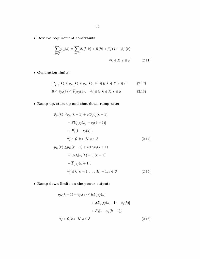
• Reserve requirement constraints:

∑j∈G

pjs(k) =∑b∈B

ds(b, k) +R(k) + β+s (k)− β−s (k)

∀k ∈ K, s ∈ S (2.11)

• Generation limits:

P jvj(k) ≤ pjs(k) ≤ pjs(k), ∀j ∈ G, k ∈ K, s ∈ S (2.12)

0 ≤ pjs(k) ≤ P jvj(k), ∀j ∈ G, k ∈ K, s ∈ S (2.13)

• Ramp-up, start-up and shut-down ramp rate:

pjs(k) ≤pjs(k − 1) +RUjvj(k − 1)

+ SUj [vj(k)− vj(k − 1)]

+ P j [1− vj(k)],

∀j ∈ G, k ∈ K, s ∈ S (2.14)

pjs(k) ≤pjs(k + 1) +RDjvj(k + 1)

+ SDj [vj(k)− vj(k + 1)]

+ P jvj(k + 1),

∀j ∈ G, k = 1, . . . , |K| − 1, s ∈ S (2.15)

• Ramp-down limits on the power output:

pjs(k − 1)− pjs(k) ≤RDjvj(k)

+ SDj [vj(k − 1)− vj(k)]

+ P j [1− vj(k − 1)],

∀j ∈ G, k ∈ K, s ∈ S (2.16)

16

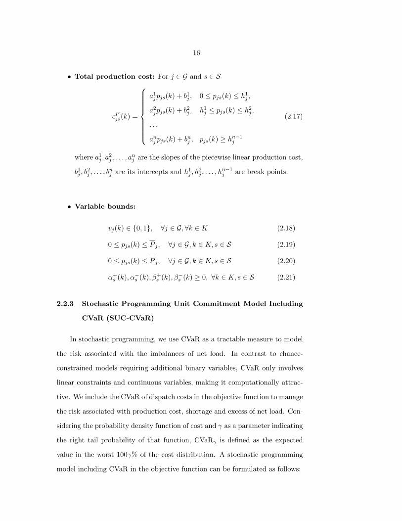
• Total production cost: For j ∈ G and s ∈ S

cPjs(k) =

a1jpjs(k) + b1j , 0 ≤ pjs(k) ≤ h1

j ,

a2jpjs(k) + b2j , h1

j ≤ pjs(k) ≤ h2j ,

. . .

anj pjs(k) + bnj , pjs(k) ≥ hn−1j

(2.17)

where a1j , a

2j , . . . , a

nj are the slopes of the piecewise linear production cost,

b1j , b2j , . . . , b

nj are its intercepts and h1

j , h2j , . . . , h

n−1j are break points.

• Variable bounds:

vj(k) ∈ 0, 1, ∀j ∈ G,∀k ∈ K (2.18)

0 ≤ pjs(k) ≤ P j , ∀j ∈ G, k ∈ K, s ∈ S (2.19)

0 ≤ pjs(k) ≤ P j , ∀j ∈ G, k ∈ K, s ∈ S (2.20)

α+s (k), α−s (k), β+

s (k), β−s (k) ≥ 0, ∀k ∈ K, s ∈ S (2.21)

2.2.3 Stochastic Programming Unit Commitment Model Including

CVaR (SUC-CVaR)

In stochastic programming, we use CVaR as a tractable measure to model

the risk associated with the imbalances of net load. In contrast to chance-

constrained models requiring additional binary variables, CVaR only involves

linear constraints and continuous variables, making it computationally attrac-

tive. We include the CVaR of dispatch costs in the objective function to manage

the risk associated with production cost, shortage and excess of net load. Con-

sidering the probability density function of cost and γ as a parameter indicating

the right tail probability of that function, CVaRγ is defined as the expected

value in the worst 100γ% of the cost distribution. A stochastic programming

model including CVaR in the objective function can be formulated as follows:

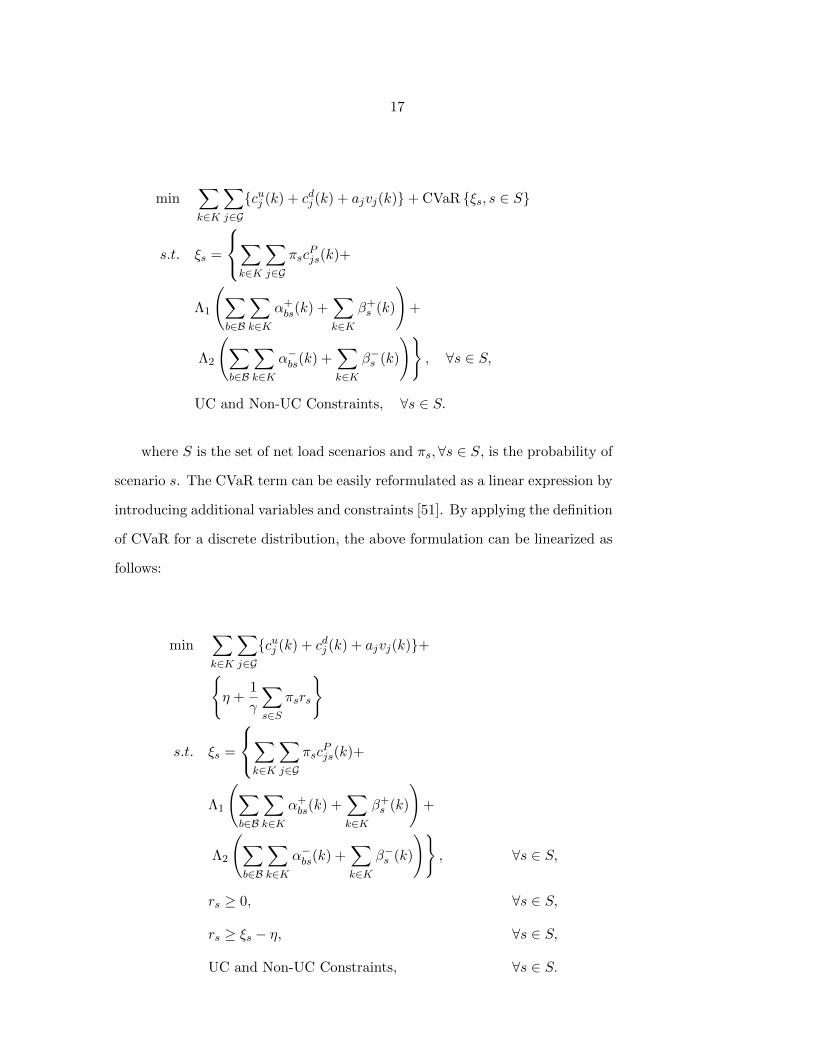
17

min∑k∈K

∑j∈Gcuj (k) + cdj (k) + ajvj(k)+ CVaR ξs, s ∈ S

s.t. ξs =

∑k∈K

∑j∈G

πscPjs(k)+

Λ1

(∑b∈B

∑k∈K

α+bs(k) +

∑k∈K

β+s (k)

)+

Λ2

(∑b∈B

∑k∈K

α−bs(k) +∑k∈K

β−s (k)

), ∀s ∈ S,

UC and Non-UC Constraints, ∀s ∈ S.

where S is the set of net load scenarios and πs,∀s ∈ S, is the probability of

scenario s. The CVaR term can be easily reformulated as a linear expression by

introducing additional variables and constraints [51]. By applying the definition

of CVaR for a discrete distribution, the above formulation can be linearized as

follows:

min∑k∈K

∑j∈Gcuj (k) + cdj (k) + ajvj(k)+

η +1

γ

∑s∈S

πsrs

s.t. ξs =

∑k∈K

∑j∈G

πscPjs(k)+

Λ1

(∑b∈B

∑k∈K

α+bs(k) +

∑k∈K

β+s (k)

)+

Λ2

(∑b∈B

∑k∈K

α−bs(k) +∑k∈K

β−s (k)

), ∀s ∈ S,

rs ≥ 0, ∀s ∈ S,

rs ≥ ξs − η, ∀s ∈ S,

UC and Non-UC Constraints, ∀s ∈ S.

18

2.2.4 Robust Unit Commitment Model (RUC)

The RUC formulation incorporates uncertainty only in terms of ranges of

the uncertain parameters. The following formulation is based on the model

presented in [8].

min∑k∈K

∑j∈Gcuj (k) + cdj (k) + ajvj(k)+

maxd∈U

∑k∈K

∑j∈G

cPj (k) +

Λ1

(∑b∈B

∑k∈K

α+b (k) +

∑k∈K

β+(k)

)+

Λ2

(∑b∈B

∑k∈K

α−b (k) +∑k∈K

β−(k)

)

s.t. UC and Non-UC Constraints ∀d ∈ U

where U is the uncertainty set of the net loads. The only uncertain parameter

in this formulation is the net load d(b, k) which consists of the net loads of each

bus b at each time period k. For this study we consider two distinct definitions

for uncertainty set. We will explain how we describe them using scenarios

in Section 2.3. Because the variables and constraints in this formulation no

longer depend on scenarios, we omitted index s from both the variables and the

constraints.

The above formulation can be recast in the following equivalent form:

miny1

∑k∈K

∑j∈Gcuj (k) + cdj (k) + ajvj(k)

+ maxd∈U

miny2∈Ω(y1,d)

∑k∈K

∑j∈G

cPj (k)+

Λ1

(∑b∈B

∑k∈K

α+b (k) +

∑k∈K

β+(k)

)+

Λ2

(∑b∈B

∑k∈K

α−b (k) +∑k∈K

β−(k)

)(2.22)

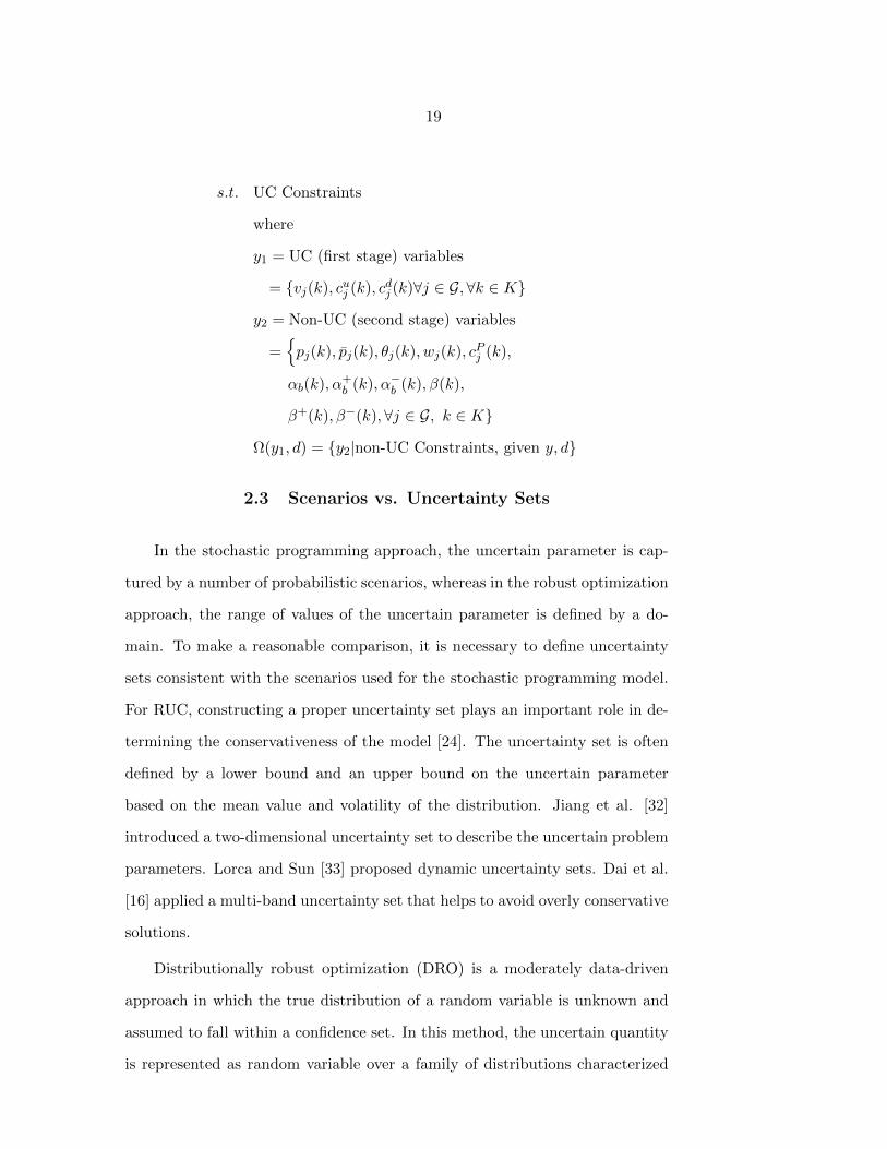
19

s.t. UC Constraints

where

y1 = UC (first stage) variables

= vj(k), cuj (k), cdj (k)∀j ∈ G, ∀k ∈ K

y2 = Non-UC (second stage) variables

=pj(k), pj(k), θj(k), wj(k), cPj (k),

αb(k), α+b (k), α−b (k), β(k),

β+(k), β−(k), ∀j ∈ G, k ∈ K

Ω(y1, d) = y2|non-UC Constraints, given y, d

2.3 Scenarios vs. Uncertainty Sets

In the stochastic programming approach, the uncertain parameter is cap-

tured by a number of probabilistic scenarios, whereas in the robust optimization

approach, the range of values of the uncertain parameter is defined by a do-

main. To make a reasonable comparison, it is necessary to define uncertainty

sets consistent with the scenarios used for the stochastic programming model.

For RUC, constructing a proper uncertainty set plays an important role in de-

termining the conservativeness of the model [24]. The uncertainty set is often

defined by a lower bound and an upper bound on the uncertain parameter

based on the mean value and volatility of the distribution. Jiang et al. [32]

introduced a two-dimensional uncertainty set to describe the uncertain problem

parameters. Lorca and Sun [33] proposed dynamic uncertainty sets. Dai et al.

[16] applied a multi-band uncertainty set that helps to avoid overly conservative

solutions.

Distributionally robust optimization (DRO) is a moderately data-driven

approach in which the true distribution of a random variable is unknown and

assumed to fall within a confidence set. In this method, the uncertain quantity

is represented as random variable over a family of distributions characterized

20

by its descriptive statistics. The advantage of this method is being based on

the historical data and its solutions are robust to distributional assumptions.

However, it is less conservative and also requires more information to derive

descriptive statistics. An example of a DRO model for UC considering uncer-

tain wind power generation can be found in [78]. Gourtani et. al. applied a

distributionally robust modeling framework for the unit commitment problem

with supply uncertainty with n− 1 security criteria [23]. Zhang et. al. formu-

late a chance constrained optimal power flow problem to procure minimum cost

energy, generator reserves, and load reserves given uncertainty in renewable en-

ergy production, load consumption, and load reserve capacities and solve it with

DRO, which ensures that chance constraints are satisfied for any distribution

in a confidence set [80]. Zhao et. al constructed the confidence sets utilizing

the L1 norm and L∞ norm in a data-driven environment [82].

In this study, we consider two approaches to develop the uncertainty sets.

The first approach is to assume the net load for each time period at each

node falls between a lower and an upper bound, which can be set by certain

percentiles of the random load output based on historical data [8, 81]. Note that

a scenario specifies the net load for each hour and each bus in the scheduling

horizon. A parameter called the budget of uncertainty is defined to control the

deviation of all loads from their nominal values. According to [8] the uncertainty

set can be described as follows:

U1 :=

dkb :∑b∈Nd

|dkb − dkb |dkb

≤ ∆k, dkb ∈ [dkb − dkb , dkb + dkb ],

∀b ∈ Nd,∀k ∈ K

where Nd is the set of buses that have uncertain load, dkb is the nominal value

of load and dkb is the maximum possible deviation of load of bus b at time k

from the nominal value. The parameter ∆k is the budget of uncertainty, taking

values between 0 and |Nd|. When ∆k = 0, the robust formulation corresponds

to the deterministic case. As ∆k increases, the uncertainty set enlarges, which

21

results in more conservative UC solutions. The maximum amount of deviation

that can be considered for the net load in each period is |Nd|.

Our second approach is to construct uncertainty sets using historical re-

alizations of the random variables by applying a connection between convex

sets and a specific class of risk measures [7]. It is proved that a constraint

with a coherent risk measure can be equivalently written as a constraint with

a corresponding convex uncertainty set [7]. In other words, we can formulate

the optimization problem with uncertain data as a robust optimization problem

with a convex uncertainty set related to a coherent risk measure. This risk mea-

sure expresses the decision maker’s risk preference. We apply the link between

CVaR as a coherent risk measure and polyhedral uncertainty sets to define an

uncertainty set based on scenarios. Enforcing a constraint in which CVaRα of

a term is less than or equal to zero roughly means that the expected value of

that term, in the 100 α% worst cases, is no less than zero. Here α = r/N where

r and N are described in the following.

Given N data points; i.e., s1, s2, . . . , sN , the uncertainty set corresponding

to CVaRα is

U2 := conv

(1

α

∑i∈I

πisi + (1− 1

α

∑i∈I

πi)sj :

I ⊆ 1, . . . , N, j ∈ 1, . . . , N \ I,∑i∈I

πi ≤ α

),

where conv(·) denotes the convex hull.

Assuming the probability distribution of sample points si as πi = 1/N ,

each of which represents one observation of demand d(b, k), and considering

α = r/N for some r ∈ Z+, this has the interpretation of the convex hull of all

r-point averages the demand observations. Let

F :=

1

α

∑i∈I

πisi + (1− 1

α

∑i∈I

πi)sj :

I ⊆ 1, . . . , N, j ∈ 1, . . . , N \ I,∑i∈I

πi ≤ α

.

22

be the set of all possible points for a certain α value. Because F has finitely

many elements, we can write it as F = f1, . . . , fm for some finite m. To

define the uncertainty set, we introduce a decision variable µi corresponding to

each fi, i = 1, . . . ,m. Since each scenario has dimension |B|× |K|, the elements

of the uncertainty set are represented as f b,ki . The convex hull term in the

definition of U2 can be formulated as the following:

U2 :=

(µ, d) ∈ Rm × R|B|×|K| :m∑i=1

µifb,ki = db,k,∀b, k,

m∑i=1

µi = 1, µi ≥ 0, i = 1, . . . ,m.

Here, the parameter α takes values between 0 and 1. As α decreases,

the uncertainty set enlarges, so that the resulting robust solutions are more

conservative and the system is protected against a higher degree of uncertainty.

2.4 Numerical Experiments

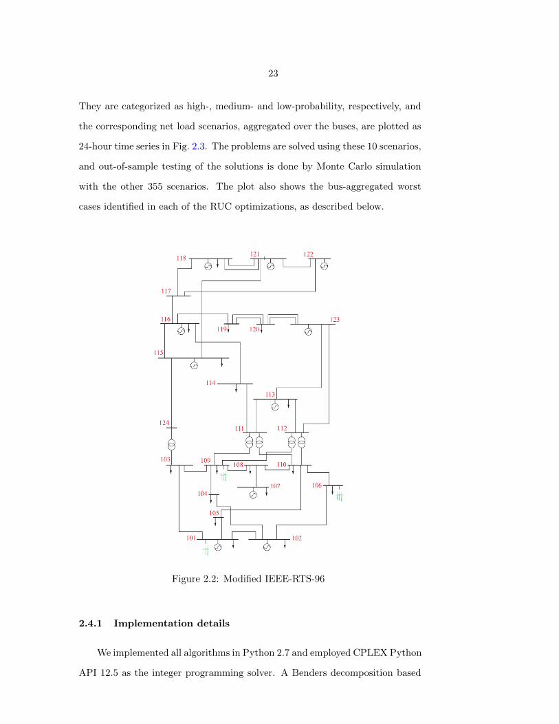
To test the approaches, we adopted the modified 24-bus IEEE RTS-96

system [74] with 32 generators and 38 transmission lines using data from [4].

The power system network is displayed in Figure 2.2. The data set includes

hourly demand data for one year. Three wind farms are added to the grid as

in [44] with wind scenarios extracted from the NREL wind data sets [3]. The

penalty cost coefficients were arbitrarily set with values of Λ1 = 20 $/MWh for

deficits and Λ2 = 1 $/MWh for excess. These relatively modest values allow

shortages to occur in an exaggerated way which allows comparison of risks.

They are revisited in a sensitivity study at the end of this section.

The wind data set contains 365 scenarios, assumed as equally likely. We

used the fast forward selection algorithm [27] to reduce the number of scenarios

to 10 [44]. The reduced set of scenarios included one assigned a probability

of 0.59, three with probabilities of 0.09, 0.11 and 0.12, respectively, and the

remainder with probabilities below 0.05 including two with probability 1/365.

23

They are categorized as high-, medium- and low-probability, respectively, and

the corresponding net load scenarios, aggregated over the buses, are plotted as

24-hour time series in Fig. 2.3. The problems are solved using these 10 scenarios,

and out-of-sample testing of the solutions is done by Monte Carlo simulation

with the other 355 scenarios. The plot also shows the bus-aggregated worst

cases identified in each of the RUC optimizations, as described below.

Figure 2.2: Modified IEEE-RTS-96

2.4.1 Implementation details

We implemented all algorithms in Python 2.7 and employed CPLEX Python

API 12.5 as the integer programming solver. A Benders decomposition based

24

Figure 2.3: Probabilistic scenarios and worst cases in each uncertainty set

algorithm proposed in [8] was applied to solve the RUC. We adopted a branch

and cut modification [42] for this Benders decomposition which makes it orders

of magnitude faster.

2.4.2 Results

The results of solving the problem using different approaches were evaluated

according to the costs of optimally dispatching the committed units in the out-

of-sample simulation. Total costs include dispatch and unit commitment cost:

Total Cost = Dispatch Cost + Unit Commitment Cost,

where

Dispatch Cost = Production Cost + Penalty Cost.

The production cost is computed from Equation (7) as:

Production Cost =∑j∈G

∑k∈K

cPj (k).

We also compute the penalties of deficit and excess of demand requirements as

Penalty Cost = Λ1

∑k∈K

∑b∈B

α+b (k) + Λ2

∑k∈K

∑b∈B

α−b (k).

25

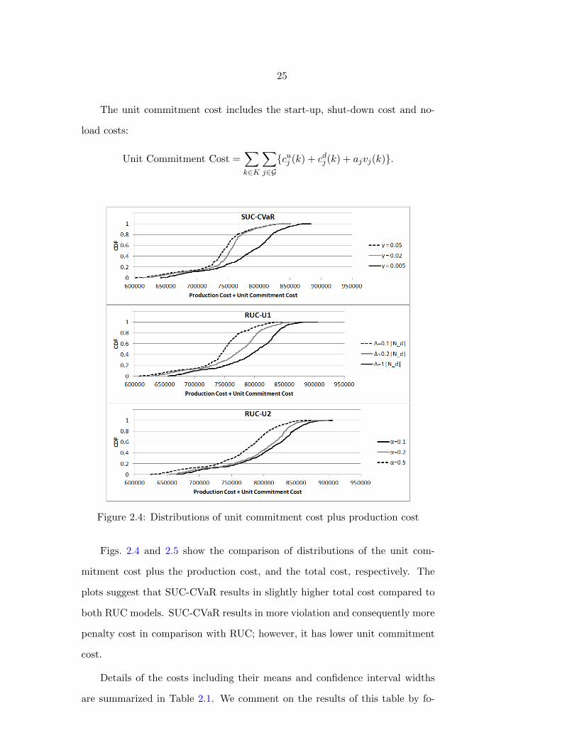
The unit commitment cost includes the start-up, shut-down cost and no-

load costs:

Unit Commitment Cost =∑k∈K

∑j∈Gcuj (k) + cdj (k) + ajvj(k).

Figure 2.4: Distributions of unit commitment cost plus production cost

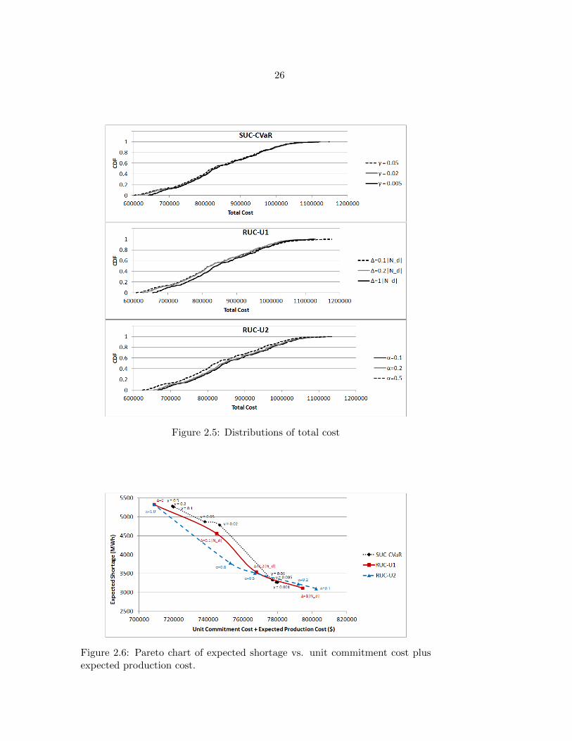
Figs. 2.4 and 2.5 show the comparison of distributions of the unit com-

mitment cost plus the production cost, and the total cost, respectively. The

plots suggest that SUC-CVaR results in slightly higher total cost compared to

both RUC models. SUC-CVaR results in more violation and consequently more

penalty cost in comparison with RUC; however, it has lower unit commitment

cost.

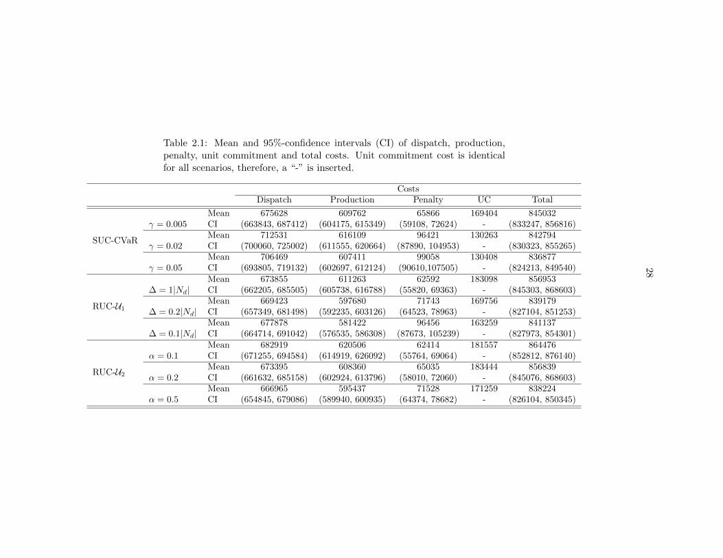
Details of the costs including their means and confidence interval widths

are summarized in Table 2.1. We comment on the results of this table by fo-

26

Figure 2.5: Distributions of total cost

Figure 2.6: Pareto chart of expected shortage vs. unit commitment cost plusexpected production cost.

27

cusing on settings for each approach with almost equal expected total cost;

i.e., SUC-CVaR with γ = 0.05, RUC-U1 with ∆ = 0.2|Nd| and RUC-U2 with

α = 0.5. The unit commitment cost of SUC-CVaR is significantly lower than

in both RUC formulations. In fact, two generators that were never commit-

ted by SUC were kept operating continuously by both RUC models. However,

SUC-CVaR’s expected penalty cost is about 30% higher than those of the RUC

models. SUC-CVaR has higher expected production cost than RUC-U2 with

95% confidence, but its production cost confidence interval overlaps with that

of RUC-U1. Overall, the cost comparison indicates that the SUC-CVaR empha-

sizing the 5% tail is less conservative than the RUC formulations. To compare

uncertainty sets U1 and U2, one can see that although the unit commitment cost

of RUC-U2 with α = 0.5 is higher than the unit commitment cost of RUC-U1

with ∆ = 0.2|Nd|, RUC-U2 results in less violation and, therefore, it is more

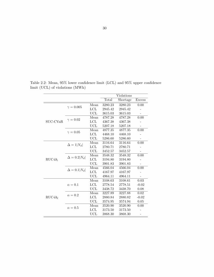
reliable. This conclusion is reinforced by Table 2.2, which contains mean and

confidence intervals of the violation of constraints (3).

The level of conservatism can be adjusted in all three methods by adjust-

ing the extent of the uncertainty sets considered in the RUC formulations or

the tail probability in the SUC-CVaR formulation. Fig. 2.6 presents a Pareto

chart to illustrate the tradeoff between cost and reliability. It indicates that,

if a decision-maker emphasizes cost by setting ∆ small, or α or γ large, then

the data-driven RUC-U2 achieves the most efficient combinations of expected

cost and expected shortage. When these parameters are adjusted for higher

conservatism, RUC-U1 dominates. But at the most stringent risk-minimizing

parameter settings, the CVaR-adjusted SUC formulation may achieve a better

cost-reliability tradeoff than either RUC formulation. Because the confidence

intervals on the expected cost and shortage values overlap, these findings should

be verified in more extensive numerical tests using the particular system pa-

rameters and penalty values chosen by the system operator.

28

Table 2.1: Mean and 95%-confidence intervals (CI) of dispatch, production,penalty, unit commitment and total costs. Unit commitment cost is identicalfor all scenarios, therefore, a “-” is inserted.

CostsDispatch Production Penalty UC Total

SUC-CVaR

γ = 0.005Mean 675628 609762 65866 169404 845032CI (663843, 687412) (604175, 615349) (59108, 72624) - (833247, 856816)

γ = 0.02Mean 712531 616109 96421 130263 842794CI (700060, 725002) (611555, 620664) (87890, 104953) - (830323, 855265)

γ = 0.05Mean 706469 607411 99058 130408 836877CI (693805, 719132) (602697, 612124) (90610,107505) - (824213, 849540)

RUC-U1

∆ = 1|Nd|Mean 673855 611263 62592 183098 856953CI (662205, 685505) (605738, 616788) (55820, 69363) - (845303, 868603)

∆ = 0.2|Nd|Mean 669423 597680 71743 169756 839179CI (657349, 681498) (592235, 603126) (64523, 78963) - (827104, 851253)

∆ = 0.1|Nd|Mean 677878 581422 96456 163259 841137CI (664714, 691042) (576535, 586308) (87673, 105239) - (827973, 854301)

RUC-U2

α = 0.1Mean 682919 620506 62414 181557 864476CI (671255, 694584) (614919, 626092) (55764, 69064) - (852812, 876140)

α = 0.2Mean 673395 608360 65035 183444 856839CI (661632, 685158) (602924, 613796) (58010, 72060) - (845076, 868603)

α = 0.5Mean 666965 595437 71528 171259 838224CI (654845, 679086) (589940, 600935) (64374, 78682) - (826104, 850345)

29

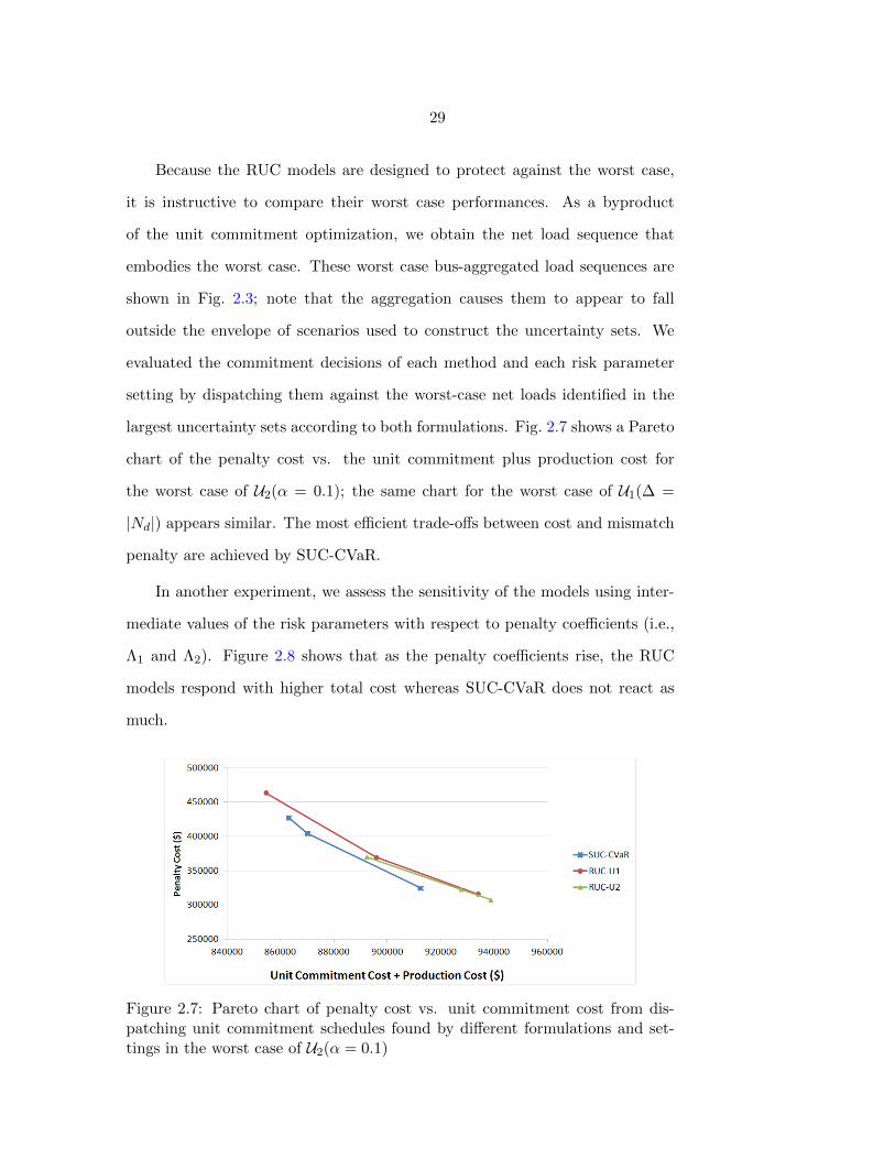
Because the RUC models are designed to protect against the worst case,

it is instructive to compare their worst case performances. As a byproduct

of the unit commitment optimization, we obtain the net load sequence that

embodies the worst case. These worst case bus-aggregated load sequences are

shown in Fig. 2.3; note that the aggregation causes them to appear to fall

outside the envelope of scenarios used to construct the uncertainty sets. We

evaluated the commitment decisions of each method and each risk parameter

setting by dispatching them against the worst-case net loads identified in the

largest uncertainty sets according to both formulations. Fig. 2.7 shows a Pareto

chart of the penalty cost vs. the unit commitment plus production cost for

the worst case of U2(α = 0.1); the same chart for the worst case of U1(∆ =

|Nd|) appears similar. The most efficient trade-offs between cost and mismatch

penalty are achieved by SUC-CVaR.

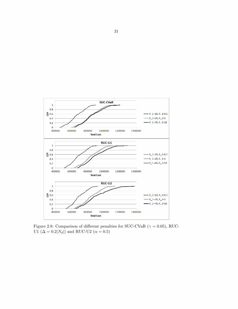
In another experiment, we assess the sensitivity of the models using inter-

mediate values of the risk parameters with respect to penalty coefficients (i.e.,

Λ1 and Λ2). Figure 2.8 shows that as the penalty coefficients rise, the RUC

models respond with higher total cost whereas SUC-CVaR does not react as

much.

Figure 2.7: Pareto chart of penalty cost vs. unit commitment cost from dis-patching unit commitment schedules found by different formulations and set-tings in the worst case of U2(α = 0.1)

30

Table 2.2: Mean, 95% lower confidence limit (LCL) and 95% upper confidencelimit (UCL) of violations (MWh)

ViolationsTotal Shortage Excess

SUC-CVaR

γ = 0.005Mean 3280.23 3280.23 0.00LCL 2945.42 2945.42 -UCL 3615.03 3615.03 -

γ = 0.02Mean 4787.28 4787.28 0.00LCL 4367.38 4367.38 -UCL 5207.18 5207.18 -

γ = 0.05Mean 4877.35 4877.35 0.00LCL 4468.10 4468.10 -UCL 5286.60 5286.60 -

RUC-U1

∆ = 1|Nd|Mean 3116.64 3116.64 0.00LCL 2780.71 2780.71 -UCL 3452.57 3452.57 -

∆ = 0.2|Nd|Mean 3548.32 3548.32 0.00LCL 3194.80 3194.80 -UCL 3901.83 3901.83 -

∆ = 0.1|Nd|Mean 4566.04 4566.04 0.00LCL 4167.97 4167.97 -UCL 4964.11 4964.11 -

RUC-U2

α = 0.1Mean 3108.63 3108.61 0.03LCL 2778.54 2778.51 -0.02UCL 3438.72 3438.70 0.08

α = 0.2Mean 3227.89 3227.88 0.02LCL 2880.84 2880.82 -0.02UCL 3574.95 3574.94 0.05

α = 0.5Mean 3520.90 3520.90 0.00LCL 3173.50 3173.50 -UCL 3868.30 3868.30 -

31

Figure 2.8: Comparison of different penalties for SUC-CVaR (γ = 0.05), RUC-U1 (∆ = 0.2|Nd|) and RUC-U2 (α = 0.5)

32

2.5 Conclusions

Robust optimization and stochastic programming have been extensively

discussed and studied as alternatives to optimize unit commitment schedules

under uncertainty. A popular impression has arisen that the robust approach,

with its focus on the worst case, is better able to control risk while stochastic

programming emphasizes expected values. However, the stochastic program-

ming formulation can easily accommodate a risk measure. Moreover, the results

of both methods depend strongly on the model for the uncertain parameters

– either the uncertainty set or the probabilistic scenarios employed in the op-

timization. To compare both approaches on the same information basis, we

constructed uncertainty sets by two methods based on the same reduced set

of scenarios used in the stochastic programming formulation. The schedules

found by each approach for various risk parameter values were evaluated in an

out-of-sample simulation.

The numerical results indicate that the cost-risk trade-off achieved by any

approach is strongly influenced by the value of its respective risk parameter. By

incorporating risk in the stochastic programming formulation in terms of CVaR

with a sufficiently low tail probability, the stochastic programming formulation

can achieve the most efficient combinations of cost and risk. Notably, it provides

schedules that perform best should the worst case (determined according to

either uncertainty set) occur. Between the two uncertainty set formulations for

robust optimization, the data-driven method that incorporates probabilities of

scenarios as well as their ranges of values achieves better cost-risk trade-offs

than the one based on ranges alone.

33

CHAPTER 3. IMPROVING SOLUTION METHODS FOR

ROBUST UNIT COMMITMENT

3.1 Introduction

Unit commitment (UC) is a problem that must be solved frequently by a

power utility or system operator to determine an economic schedule of which

units will be used to meet the forecast demand and operating constraints over a

short time horizon. For example, the California Independent System Operator

considers a one-hour time period between 10:00 a.m. and 11:00 a.m. on the day

before the targeted day to receive and evaluate bids from market participants,

solve the UC problem, and publish the results [2]. Hence, it is crucial to be

able to solve the problem by the end of the period.

The UC problem is a mixed-integer programming problem that uses binary

variables to represent the commitment of generating units. Due to the use of a

large number of binary variables beside many constraints, UC is in the class of

NP-hard problems and is difficult to solve when the size of the problem becomes

large [64].

The robust unit commitment (RUC) model is one of the most studied

approaches to address uncertainties associated with renewable resources. In

the literature, RUC is mostly formulated as a two-stage programming problem

in which the first stage determines the commitment decisions and the second

stage makes dispatch decisions after the uncertainty is resolved. The RUC

problem is a multi-stage mixed-integer program and is normally difficult to

solve. Therefore, improving solution methods for this problem is of importance.

34

The process of solving RUC is a version of Benders decomposition [8]. Ben-

ders decomposition may cause a major computational bottleneck as the master

problem is solved repeatedly. The master problem is an integer program that

becomes more difficult as more inequalities are added in the course of the al-

gorithm. A number of studies have been dedicated to alleviating this problem.

Rei et al. propose a local branching approach to be used within Benders decom-

position to improve the lower and upper bounds at each iteration [49]. Saharidis

et al. introduce a new way to generate multiple cuts by solving an auxiliary

problem based on the solution of the master problem. They show that this

methodology significantly decreases the number of iterations and the compu-

tational time [57]. Saharidis and Ierapetritou presented a maximum feasible

subsystem cut generation approach where at each iteration of the Benders al-

gorithm, an extra cut is generated to restrict the value of the objective function

of the master problem. This strategy focuses on the particular case where more

feasibility than optimality Benders cuts are produced. The proposed algorithm

was shown to significantly reduce the computational time [58].

In this study, we apply a branch-and-cut algorithm presented in [42] for

integer programs based on Benders decomposition. Branch-and-cut, one of the

main solution methodologies for mixed integer programming, is a combination

of branch-and-bound and cutting plane approaches. In the branch-and-cut al-

gorithm, a linear relaxation is solved at each node of the branch-and-bound

tree. Valid cuts are added to eliminate integer solutions that violate the re-

laxed constraints. After adding inequalities, if the solutions remain fractional,

branching is performed.

We implement this method on a UC formulation based on [13]. An al-

ternative formulation to the deterministic UC which is widely recognized to be

more efficient is presented by [40]. However, the implementation of this method

would be the same on the alternative formulation and it could be explored to

show improvement.

35

This chapter is organized as follows. In Section 3.2 we explain the solution

method for the robust optimization formulation which is adopted from Bertsi-

mas et al. [8]. In Section 3.3 we propose a branch-and-cut algorithm to improve

the solution methods for this robust unit commitment problem. We also pro-

vide the details of the subproblems and inequalities used to solve the RUC in

Section 3.4. Computational results are summarized in Section 3.5. Finally, we

conclude this Chapter in Section 3.6.

3.2 The Existing Method

In this section, a variant of Benders decomposition [8] is applied for the

proposed robust optimization unit commitment problem. We first present the

RUC formulation. We write y1 for the UC variables that are independent of

uncertainty; i.e., the unit commitment, start-up and shut-down cost variables.

Also, we write y2 for the dispatch variables (recall that the dispatch variables

may depend on the values of uncertain parameters, e.g. power output, phase

angle, production cost). The uncertain parameters (in our problem, the hourly

net load) can vary on a set denoted as D. The RUC is then summarized as

miny1,y2

(cT y1 + max

d∈DbT y2(d)

)(3.1a)

s.t. Fy1 ≤ f , (3.1b)

Hy2(d) ≤ h, d ∈ D (3.1c)

Ay1 + By2(d) ≤ g, d ∈ D (3.1d)

Ey2(d) = d, d ∈ D (3.1e)

y1 ∈ Rn1 × 0, 1p1 , (3.1f)

y2(d) ∈ Rn2 , d ∈ D. (3.1g)

In Problem (3.1), the objective function (3.1a) minimizes a combination of unit

commitment costs, such as start-up and shut-down costs, and the worst case

of the dispatch costs, such as production and shortage costs. Constraint (3.1b)

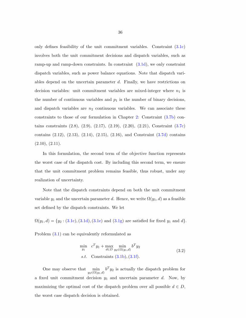
36

only defines feasibility of the unit commitment variables. Constraint (3.1c)

involves both the unit commitment decisions and dispatch variables, such as

ramp-up and ramp-down constraints. In constraint (3.1d), we only constraint

dispatch variables, such as power balance equations. Note that dispatch vari-

ables depend on the uncertain parameter d. Finally, we have restrictions on

decision variables: unit commitment variables are mixed-integer where n1 is

the number of continuous variables and p1 is the number of binary decisions,

and dispatch variables are n2 continuous variables. We can associate these

constraints to those of our formulation in Chapter 2: Constraint (3.7b) con-

tains constraints (2.8), (2.9), (2.17), (2.19), (2.20), (2.21), Constraint (3.7c)

contains (2.12), (2.13), (2.14), (2.15), (2.16), and Constraint (3.7d) contains

(2.10), (2.11).

In this formulation, the second term of the objective function represents

the worst case of the dispatch cost. By including this second term, we ensure

that the unit commitment problem remains feasible, thus robust, under any

realization of uncertainty.

Note that the dispatch constraints depend on both the unit commitment

variable y1 and the uncertain parameter d. Hence, we write Ω(y1, d) as a feasible

set defined by the dispatch constraints. We let

Ω(y1, d) = y2 : (3.1c), (3.1d), (3.1e) and (3.1g) are satisfied for fixed y1 and d.

Problem (3.1) can be equivalently reformulated as

miny1

cT y1 + maxd∈D

miny2∈Ω(y1,d)

bT y2

s.t. Constraints (3.1b), (3.1f).

(3.2)

One may observe that miny2∈Ω(y1,d)

bT y2 is actually the dispatch problem for

a fixed unit commitment decision y1 and uncertain parameter d. Now, by

maximizing the optimal cost of the dispatch problem over all possible d ∈ D,

the worst case dispatch decision is obtained.

37

To solve Problem (3.2), we reformulate it as follows:

miny1,γ

cT y1 + γ

s.t. (3.1b), (3.1f)

γ ≥ S(y1, d), ∀ d ∈ D,

(3.3)

where

S(y1, d) = miny2∈Ω(y1,d)

bT y2. (3.4)

We write R(y1) as the worst case of the dispatch problem:

R(y1) = maxd∈D

S(y1, d). (3.5)

Note that in our problem formulation, since R(y1) represents the worst case

dispatch cost, we write γ ≥ 0 without loss of optimality. This problem can be

then reformulated as

miny1,γ

cT y1 + γ

s.t. (3.1b), (3.1f)

γ ≥ R(y1),

γ ≥ 0.

(3.6)

Problem (3.6) is solved using a Benders decomposition approach. In the

following two sections, we present how to solve subproblem (3.5) and master

problem (3.6).

3.2.1 Outer approximation to evaluate R(y1)

For given y1 and d

S(y1, d) = miny2

bT y2 (3.7a)

s.t. Hy2 ≤ h, (3.7b)

By2 ≤ −Ay1 + g, (3.7c)

Ey2 = d, (3.7d)

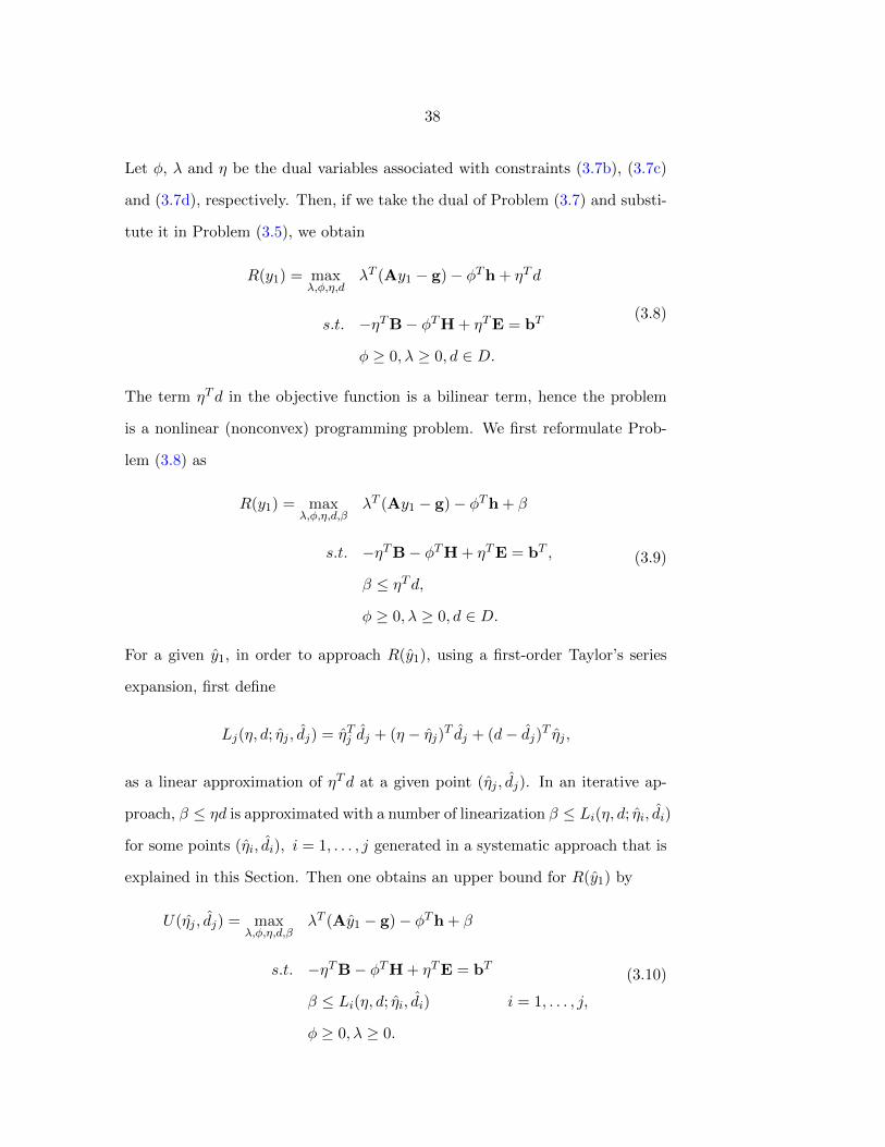
38

Let φ, λ and η be the dual variables associated with constraints (3.7b), (3.7c)

and (3.7d), respectively. Then, if we take the dual of Problem (3.7) and substi-

tute it in Problem (3.5), we obtain

R(y1) = maxλ,φ,η,d

λT (Ay1 − g)− φTh + ηTd

s.t. −ηTB− φTH + ηTE = bT

φ ≥ 0, λ ≥ 0, d ∈ D.

(3.8)

The term ηTd in the objective function is a bilinear term, hence the problem

is a nonlinear (nonconvex) programming problem. We first reformulate Prob-

lem (3.8) as

R(y1) = maxλ,φ,η,d,β

λT (Ay1 − g)− φTh + β

s.t. −ηTB− φTH + ηTE = bT ,

β ≤ ηTd,

φ ≥ 0, λ ≥ 0, d ∈ D.

(3.9)

For a given y1, in order to approach R(y1), using a first-order Taylor’s series

expansion, first define

Lj(η, d; ηj , dj) = ηTj dj + (η − ηj)T dj + (d− dj)T ηj ,

as a linear approximation of ηTd at a given point (ηj , dj). In an iterative ap-

proach, β ≤ ηd is approximated with a number of linearization β ≤ Li(η, d; ηi, di)

for some points (ηi, di), i = 1, . . . , j generated in a systematic approach that is

explained in this Section. Then one obtains an upper bound for R(y1) by

U(ηj , dj) = maxλ,φ,η,d,β

λT (Ay1 − g)− φTh + β

s.t. −ηTB− φTH + ηTE = bT

β ≤ Li(η, d; ηi, di) i = 1, . . . , j,

φ ≥ 0, λ ≥ 0.

(3.10)

39

Also, for a given d ∈ D, a lower bound can be achieved by

S(y1, d) = maxλ,φ,η

λT (Ay1 − g)− φTh + ηT d

s.t. −ηTB− φTH + ηTE = bT

φ ≥ 0, λ ≥ 0.

Note that this is a LP because d is no longer a decision variable. The solution

of this problem is feasible for (3.8), hence yields a lower bound.

The steps to evaluate R(y1) for a given y1 are then summarized in Algo-

rithm 1.

1 Algorithm: Evaluate R(y1)

2 Let j := 1, UOA = +∞, and LOA = −∞. Choose a feasible dj ∈ D and a

small tolerance δ > 0.

3 while UOA − LOA > δ do

4 Evaluate S(y1, dj). Let (φj , λj , ηj) be the optimal solution.

5 LOA = maxLOA, S(y1, dj).6 Define the linearization Lj(η, d; ηj , dj) and update U(ηj , dj) with it.

7 Evaluate U(ηj , dj).

8 Denote (φj+1, λj+1, ηj+1, βj+1, dj+1) the solution.

9 Update UOA = U(ηj , dj).

10 j := j + 1.

11 Return (φj , λj , ηj , dj) as the solution and S(y1, dj) as the value.

Algorithm 1: Outer approximation approach to evaluate R(y1)

Algorithm 1, called the outer approximation algorithm, is a well-known

method in nonlinear and mixed-integer nonlinear programming ([17], [21], [25]).

Using a Taylor’s series expansion to outer approximate the nonlinear functions,

a relaxed linear set is obtained for the original nonlinear feasible set. This lin-

ear set is then refined by adding further linearizations at other points generated

during the course of the algorithm. Because we run this algorithm until the

lower and upper bounds meet within a small tolerance δ, the method converges

to an optimal solution. However, since R(y1) is nonconcave, only a local opti-

mum is guaranteed. The reason why it is called an approximation is because

40

the actual nonlinear term ηTd is replaced with linear approximations. Note

that in our case, since the problem is a maximization, optimizing the objective

function over the relaxed linear set will yield an upper bound.

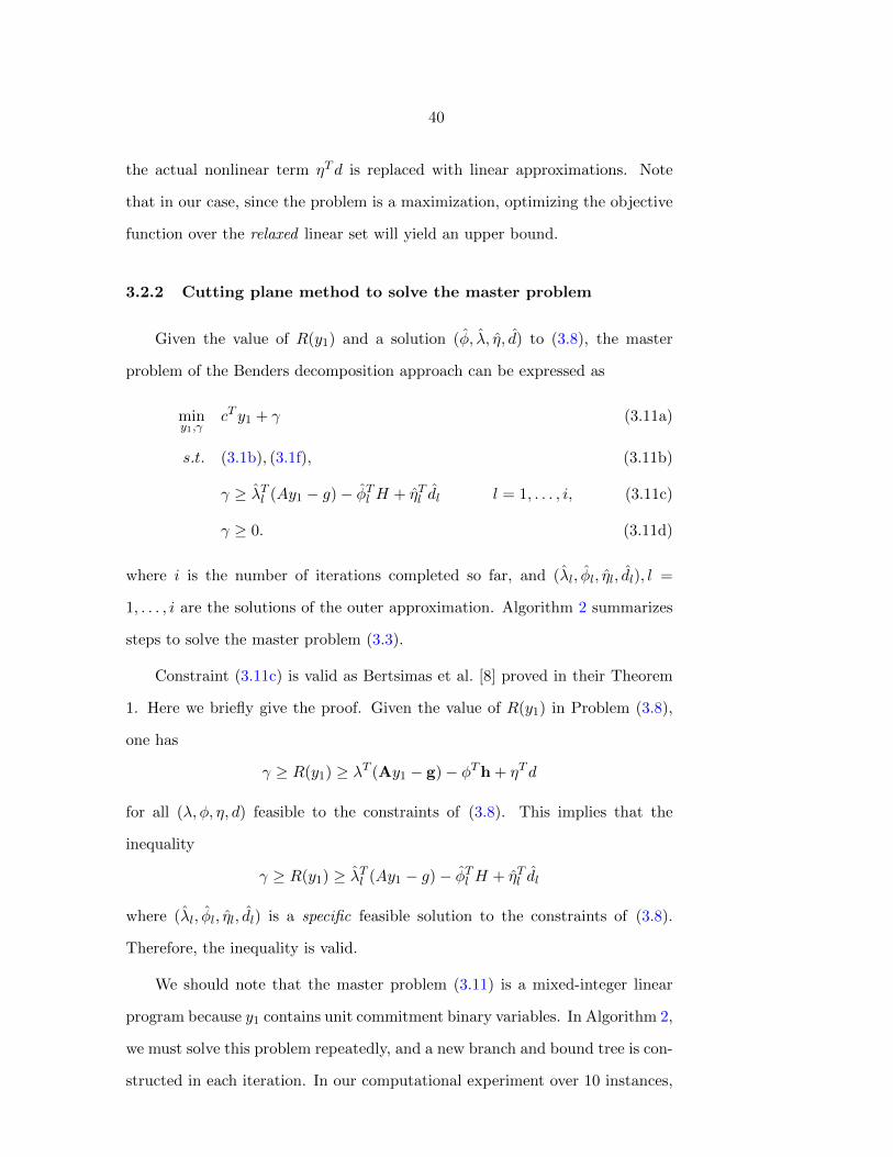
3.2.2 Cutting plane method to solve the master problem

Given the value of R(y1) and a solution (φ, λ, η, d) to (3.8), the master

problem of the Benders decomposition approach can be expressed as

miny1,γ

cT y1 + γ (3.11a)

s.t. (3.1b), (3.1f), (3.11b)

γ ≥ λTl (Ay1 − g)− φTl H + ηTl dl l = 1, . . . , i, (3.11c)

γ ≥ 0. (3.11d)

where i is the number of iterations completed so far, and (λl, φl, ηl, dl), l =

1, . . . , i are the solutions of the outer approximation. Algorithm 2 summarizes

steps to solve the master problem (3.3).

Constraint (3.11c) is valid as Bertsimas et al. [8] proved in their Theorem

1. Here we briefly give the proof. Given the value of R(y1) in Problem (3.8),

one has

γ ≥ R(y1) ≥ λT (Ay1 − g)− φTh + ηTd

for all (λ, φ, η, d) feasible to the constraints of (3.8). This implies that the

inequality

γ ≥ R(y1) ≥ λTl (Ay1 − g)− φTl H + ηTl dl

where (λl, φl, ηl, dl) is a specific feasible solution to the constraints of (3.8).

Therefore, the inequality is valid.

We should note that the master problem (3.11) is a mixed-integer linear

program because y1 contains unit commitment binary variables. In Algorithm 2,

we must solve this problem repeatedly, and a new branch and bound tree is con-

structed in each iteration. In our computational experiment over 10 instances,

41

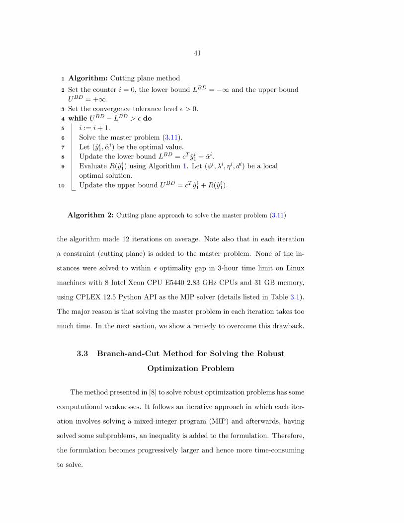
1 Algorithm: Cutting plane method

2 Set the counter i = 0, the lower bound LBD = −∞ and the upper bound

UBD = +∞.

3 Set the convergence tolerance level ε > 0.

4 while UBD − LBD > ε do

5 i := i+ 1.

6 Solve the master problem (3.11).

7 Let (yi1, αi) be the optimal value.

8 Update the lower bound LBD = cT yi1 + αi.

9 Evaluate R(yi1) using Algorithm 1. Let (φi, λi, ηi, di) be a local

optimal solution.

10 Update the upper bound UBD = cT yi1 +R(yi1).

Algorithm 2: Cutting plane approach to solve the master problem (3.11)

the algorithm made 12 iterations on average. Note also that in each iteration

a constraint (cutting plane) is added to the master problem. None of the in-

stances were solved to within ε optimality gap in 3-hour time limit on Linux

machines with 8 Intel Xeon CPU E5440 2.83 GHz CPUs and 31 GB memory,

using CPLEX 12.5 Python API as the MIP solver (details listed in Table 3.1).

The major reason is that solving the master problem in each iteration takes too

much time. In the next section, we show a remedy to overcome this drawback.

3.3 Branch-and-Cut Method for Solving the Robust

Optimization Problem

The method presented in [8] to solve robust optimization problems has some

computational weaknesses. It follows an iterative approach in which each iter-

ation involves solving a mixed-integer program (MIP) and afterwards, having

solved some subproblems, an inequality is added to the formulation. Therefore,

the formulation becomes progressively larger and hence more time-consuming

to solve.

42

Rather than solving a MIP in each iteration, we can solve the initial master

problem in a single branch-and-bound tree and in each node with an integer

feasible solution solve the underlying subproblems and add inequalities dynam-

ically to the initial formulation. By employing this approach we would need

to explore only one branch-and-bound tree. Hence, the method is likely to be

more efficient [42]. More extensive explanation follows.

We first briefly explain the standard branch-and-bound approach to solve

a mixed-integer linear program. We then show how we modify the standard

approach to solve the RUC. Suppose that we want to solve the following mixed-

integer linear program:

minx cTx

s.t. Ax ≥ b,

x ∈ Rn−p+ × Zp+

(MIP)

where n is the number of variables and p > 0 is the number of integer variables.

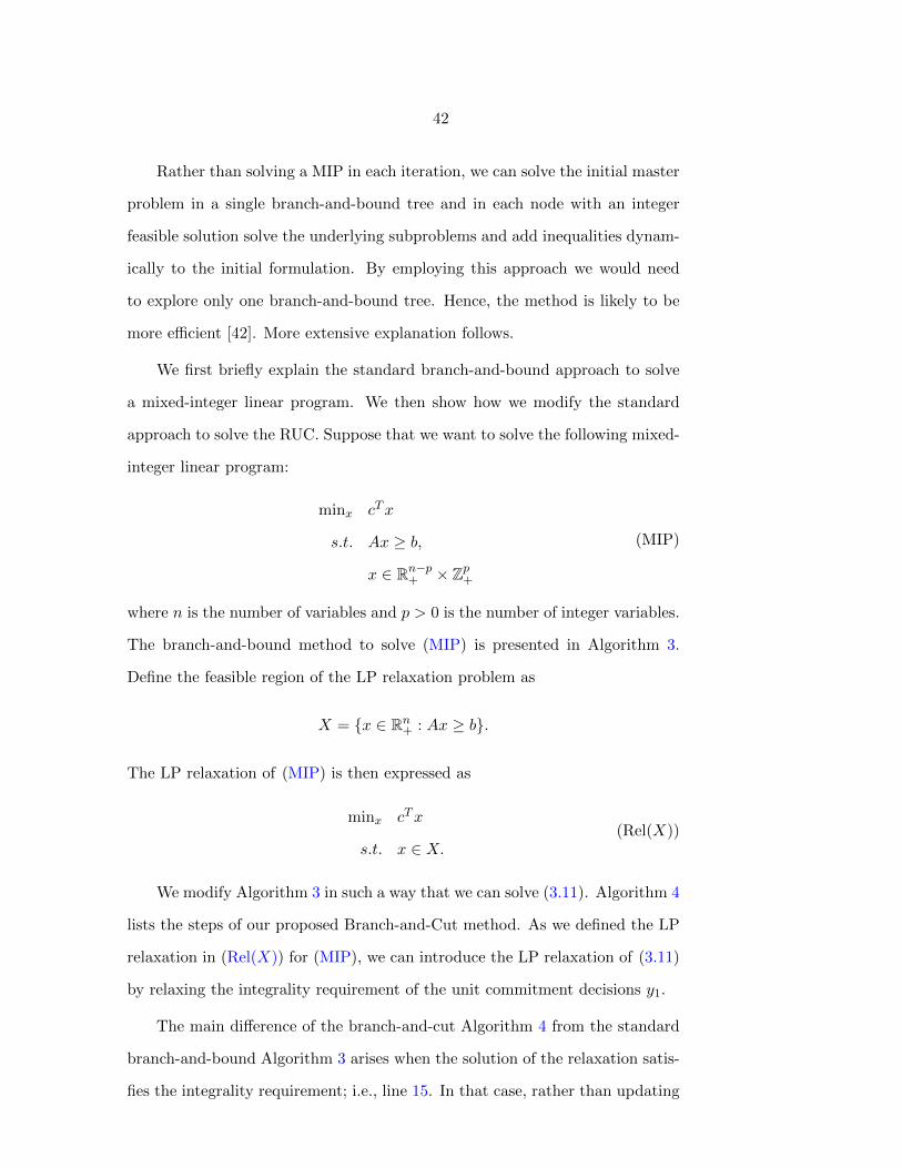
The branch-and-bound method to solve (MIP) is presented in Algorithm 3.

Define the feasible region of the LP relaxation problem as

X = x ∈ Rn+ : Ax ≥ b.

The LP relaxation of (MIP) is then expressed as

minx cTx

s.t. x ∈ X.(Rel(X))

We modify Algorithm 3 in such a way that we can solve (3.11). Algorithm 4

lists the steps of our proposed Branch-and-Cut method. As we defined the LP

relaxation in (Rel(X)) for (MIP), we can introduce the LP relaxation of (3.11)

by relaxing the integrality requirement of the unit commitment decisions y1.

The main difference of the branch-and-cut Algorithm 4 from the standard

branch-and-bound Algorithm 3 arises when the solution of the relaxation satis-

fies the integrality requirement; i.e., line 15. In that case, rather than updating

43

1 Algorithm: Branch-and-bound

2 Initialize the set of notes: N = .3 Set the lower bound LB = −∞ and the upper bound UB = +∞.

4 Let N = X be the set of nodes.

5 while N 6= ∅ do6 Select a node t from N .

7 Evaluate Rel(Xt).

8 if infeasible then

9 N = N\t.10 else

11 Let xt and zt denote the optimal solution and optimal value,

respectively.

12 if zt ≥ UB then

13 Prune the node: N = N\t.14 else if xt ∈ Rn−p+ × Zp+ then

15 UB = minUB, zt.16 N = N\t.17 else

18 Select a fractional variable xr to branch.

19 S1 := Xt ∪ x ∈ Rn+ : xr ≤ bxrt c.20 S2 := Xt ∪ x ∈ Rn+ : xr ≥ dxrt e.21 N = N ∪ S1, S2.

Algorithm 3: Branch-and-bound approach to solve (MIP)

44

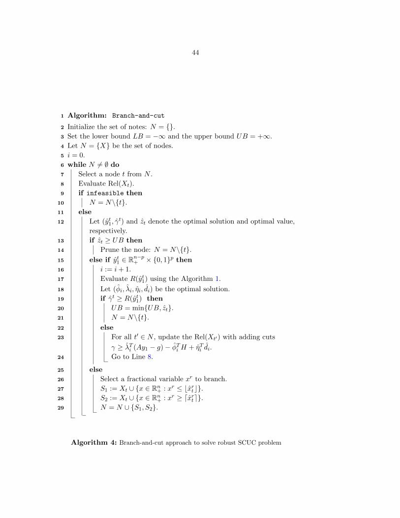
1 Algorithm: Branch-and-cut

2 Initialize the set of notes: N = .3 Set the lower bound LB = −∞ and the upper bound UB = +∞.

4 Let N = X be the set of nodes.

5 i = 0.

6 while N 6= ∅ do7 Select a node t from N .

8 Evaluate Rel(Xt).

9 if infeasible then

10 N = N\t.11 else

12 Let (yt1, γt) and zt denote the optimal solution and optimal value,

respectively.

13 if zt ≥ UB then

14 Prune the node: N = N\t.15 else if yt1 ∈ Rn−p+ × 0, 1p then

16 i := i+ 1.

17 Evaluate R(yt1) using the Algorithm 1.

18 Let (φi, λi, ηi, di) be the optimal solution.

19 if γt ≥ R(yt1) then

20 UB = minUB, zt.21 N = N\t.22 else

23 For all t′ ∈ N , update the Rel(Xt′) with adding cuts

γ ≥ λTi (Ay1 − g)− φTi H + ηTi di.

24 Go to Line 8.

25 else

26 Select a fractional variable xr to branch.

27 S1 := Xt ∪ x ∈ Rn+ : xr ≤ bxrt c.28 S2 := Xt ∪ x ∈ Rn+ : xr ≥ dxrt e.29 N = N ∪ S1, S2.

Algorithm 4: Branch-and-cut approach to solve robust SCUC problem

45

the upper bound and pruning the node, we should first check whether this so-

lution also satisfies constraint γ ≥ R(y1). If so, the solution is accepted as a

feasible solution; hence, the upper bound is updated. Otherwise, we will add

an inequality (3.11c), and then solve the LP relaxation of the same node again

with going back to Line 8. The rest of the algorithm is the same as the standard

branch-and-bound method.

The branch-and-bound tree for Algorithm 4 has a finite number of nodes,

because the formulation has only binary variables. Moreover, since the extra

steps taken to process each node are the regular Benders decomposition, and

the convergence of Benders decomposition is proved, the process of each node

is done in finite number of iterations. Hence, this branch-and-cut algorithm

converges finitely.

In our computational experiments, we implemented Algorithm 4 using the

CPLEX Python API as the underlying optimization solver. The implementa-

tion consists of three main parts as follows:

• Solving master problem (3.11). The master problem formulation (3.11),

which is a MIP problem, is defined for CPLEX using the standard ap-

proach, i.e. introducing variables, objective function and constraints to

CPLEX. To solve the master problem, CPLEX then uses its own branch-

and-bound approach, explained in Algorithm 3.

• Solving subproblem (3.9). To solve the subproblem, we implemented

the outer approximation Algorithm 1. To do so, we defined the linear pro-

gramming problems (3.10) (to evaluate U(ηj , dj)) and (3.2.1) (to evaluate

S(y1, d)) for CPLEX. Then, as explained in Algorithm 1, using a Python

code we solve these two problems iteratively until convergence.

• Adding cuts to the problem. Using the solutions of Subproblem (3.9),

we decide whether a cut is required to be added to the master problem or

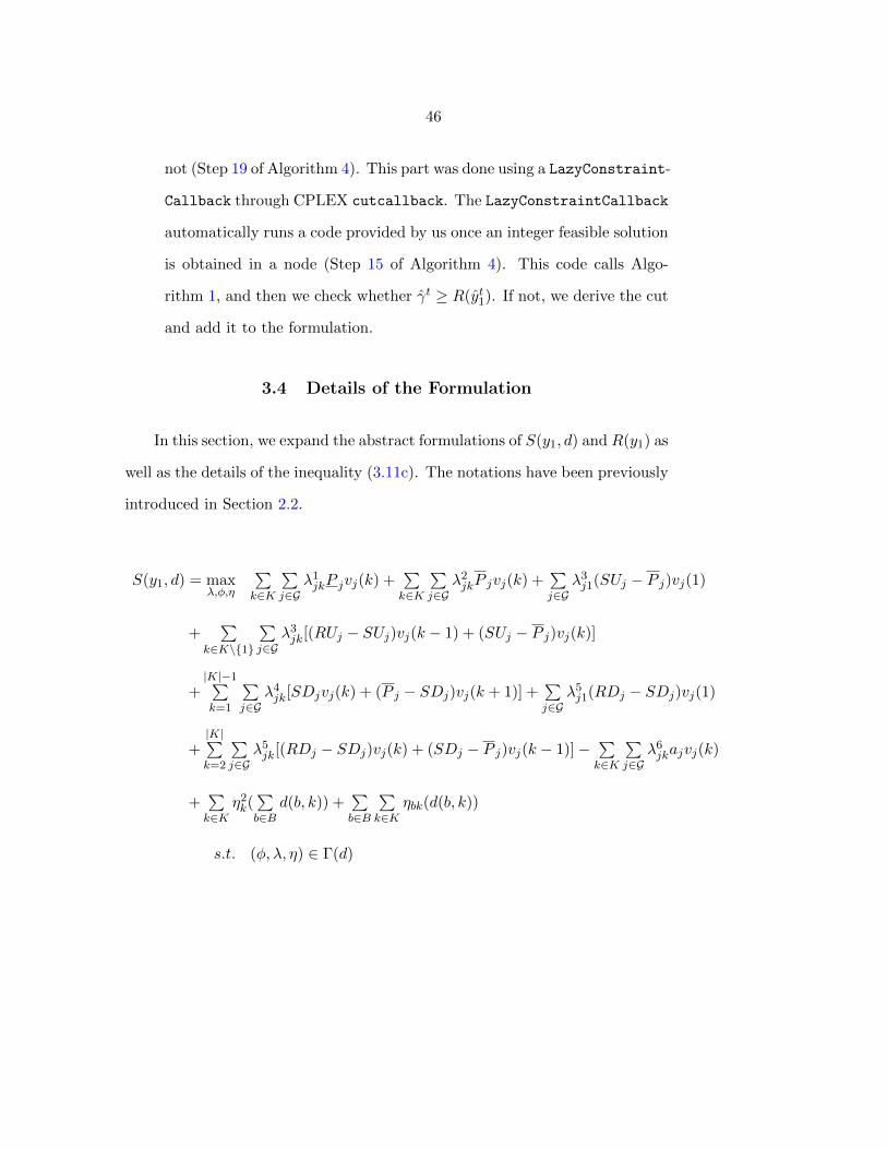
46

not (Step 19 of Algorithm 4). This part was done using a LazyConstraint-

Callback through CPLEX cutcallback. The LazyConstraintCallback

automatically runs a code provided by us once an integer feasible solution

is obtained in a node (Step 15 of Algorithm 4). This code calls Algo-

rithm 1, and then we check whether γt ≥ R(yt1). If not, we derive the cut

and add it to the formulation.

3.4 Details of the Formulation

In this section, we expand the abstract formulations of S(y1, d) and R(y1) as

well as the details of the inequality (3.11c). The notations have been previously

introduced in Section 2.2.

S(y1, d) = maxλ,φ,η

∑k∈K

∑j∈G

λ1jkP jvj(k) +

∑k∈K

∑j∈G

λ2jkP jvj(k) +

∑j∈G

λ3j1(SUj − P j)vj(1)

+∑

k∈K\1

∑j∈G

λ3jk[(RUj − SUj)vj(k − 1) + (SUj − P j)vj(k)]

+|K|−1∑k=1

∑j∈G

λ4jk[SDjvj(k) + (P j − SDj)vj(k + 1)] +

∑j∈G

λ5j1(RDj − SDj)vj(1)

+|K|∑k=2

∑j∈G

λ5jk[(RDj − SDj)vj(k) + (SDj − P j)vj(k − 1)]−

∑k∈K

∑j∈G

λ6jkajvj(k)

+∑k∈K

η2k(∑b∈B

d(b, k)) +∑b∈B

∑k∈K

ηbk(d(b, k))

s.t. (φ, λ, η) ∈ Γ(d)

47

where

Γ(d) =

(φ, λ, η) :

∑j∈G(b)

(1− ρj(k)) ηbk + λ1jk − φ6

jk + λ3j,k+1 + λ5

jk − λ5j,k+1

−bjλ6jk − φ7

jk ≤ 0, ∀j, k = 2, . . . , |K| − 1

∑j∈G(b)

(1− ρj(k)) ηbk + λ1jk − φ6

jk + λ3j,k+1 + λ5

jk − λ5j,k+1

−bjλ6jk − φ7

jk ≤ 0, ∀j, k = 1

∑j∈G(b)

(1− ρj(k)) ηbk + λ1jk − φ6

jk + λ5jk

−bjλ6jk − φ7

jk ≤ 0, ∀j, k = |K|

η2k + φ6

jk − λ2jk − λ3

jk − λ4jk − φ8

jk ≤ 0, ∀j, k = 1, . . . , |K| − 1

η2k + φ6

jk − λ2jk − λ3

jk − φ8jk ≤ 0, ∀j, k = |K|

∑`:BF (`)=1

B(`)φ1`k +

∑`:BT (`)=1

B(`)φ1`k + φ2

k + φ111k + φ12

1k = 0, ∀k

∑`:BF (`)=b

B(`)φ1`k +

∑`:BT (`)=b

B(`)φ1`k + φ11

bk + φ12bk = 0, ∀k, ∀b ≥ 2

φ1`k − η`:BF (`),k − ηBT (`),k + φ9

`k − φ10`k = 0, ∀`, k

λ6jk ≤ 1, ∀j, k

ηbk + φ3bk = 0, ∀b, k

φ4k + η2

k = 0, ∀k

−φ3bk ≤ Λ1, ∀b, k

φ3bk ≤ Λ2, ∀b, k

−φ4bk ≤ Λ1, ∀k

φ4k ≤ Λ2, ∀k

,

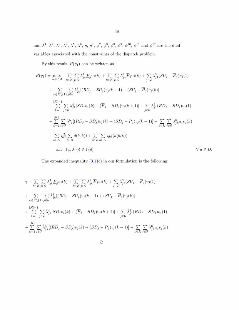
48

and λ1, λ2, λ3, λ4, λ5, λ6, η, η2, φ7, φ8, φ8, φ9, φ10, φ11 and φ12 are the dual

variables associated with the constraints of the dispatch problem.

By this result, R(y1) can be written as

R(y1) = maxλ,φ,η,d

∑k∈K

∑j∈G

λ1jkP jvj(k) +

∑k∈K

∑j∈G

λ2jkP jvj(k) +

∑j∈G

λ3j1(SUj − P j)vj(1)

+∑

k∈K\1

∑j∈G

λ3jk[(RUj − SUj)vj(k − 1) + (SUj − P j)vj(k)]

+|K|−1∑k=1

∑j∈G

λ4jk[SDjvj(k) + (P j − SDj)vj(k + 1)] +

∑j∈G

λ5j1(RDj − SDj)vj(1)

+|K|∑k=2

∑j∈G

λ5jk[(RDj − SDj)vj(k) + (SDj − P j)vj(k − 1)]−

∑k∈K

∑j∈G

λ6jkajvj(k)

+∑k∈K

η2k(∑b∈B

d(b, k)) +∑b∈B

∑k∈K

ηbk(d(b, k))

s.t. (φ, λ, η) ∈ Γ(d) ∀ d ∈ D.

The expanded inequality (3.11c) in our formulation is the following:

γ −∑k∈K

∑j∈G

λ1jkP jvj(k) +

∑k∈K

∑j∈G

λ2jkP jvj(k) +

∑j∈G

λ3j1(SUj − P j)vj(1)

+∑

k∈K\1

∑j∈G

λ3jk[(RUj − SUj)vj(k − 1) + (SUj − P j)vj(k)]

+|K|−1∑k=1

∑j∈G

λ4jk[SDjvj(k) + (P j − SDj)vj(k + 1)] +

∑j∈G

λ5j1(RDj − SDj)vj(1)

+|K|∑k=2

∑j∈G

λ5jk[(RDj − SDj)vj(k) + (SDj − P j)vj(k − 1)]−

∑k∈K

∑j∈G

λ6jkajvj(k)

≥

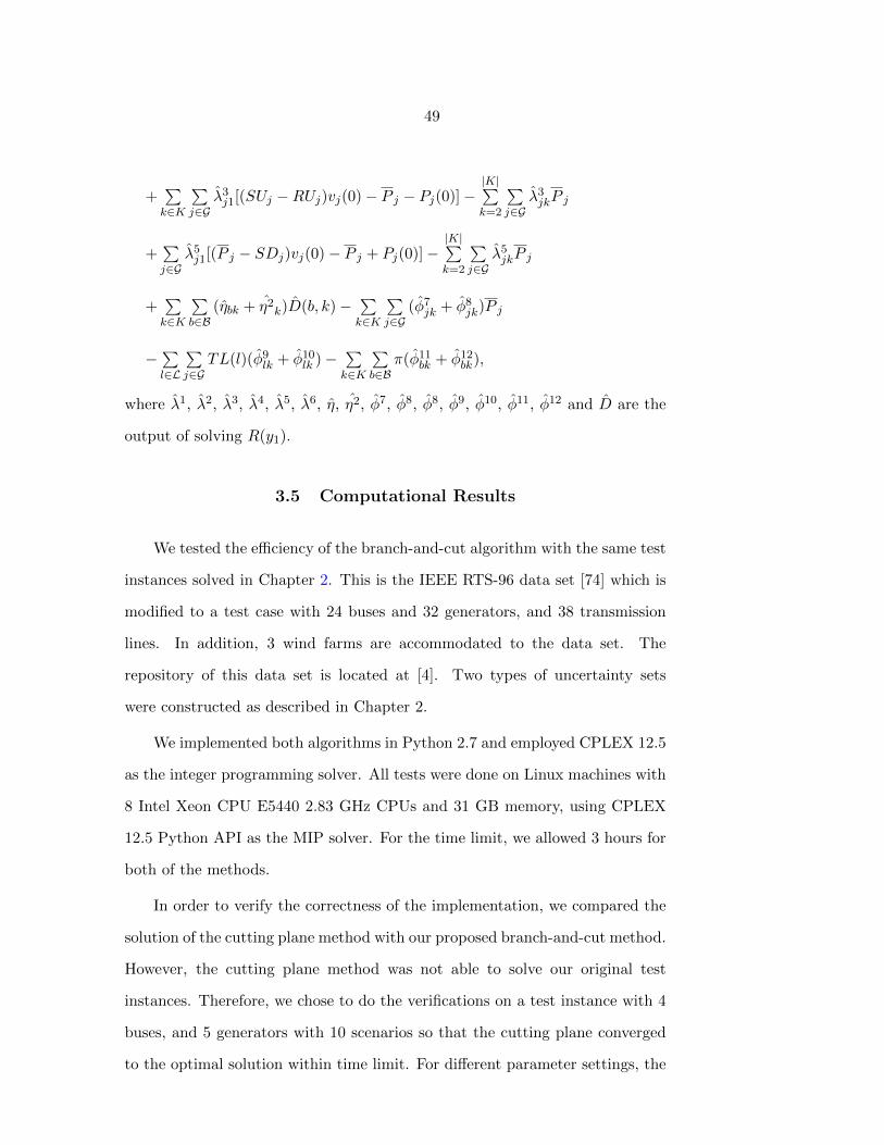
49

+∑k∈K

∑j∈G

λ3j1[(SUj −RUj)vj(0)− P j − Pj(0)]−

|K|∑k=2

∑j∈G

λ3jkP j

+∑j∈G

λ5j1[(P j − SDj)vj(0)− P j + Pj(0)]−

|K|∑k=2

∑j∈G

λ5jkP j

+∑k∈K

∑b∈B

(ηbk + η2k)D(b, k)−

∑k∈K

∑j∈G

(φ7jk + φ8

jk)P j

−∑l∈L

∑j∈G

TL(l)(φ9lk + φ10

lk )−∑k∈K

∑b∈B

π(φ11bk + φ12

bk),

where λ1, λ2, λ3, λ4, λ5, λ6, η, η2, φ7, φ8, φ8, φ9, φ10, φ11, φ12 and D are the

output of solving R(y1).

3.5 Computational Results

We tested the efficiency of the branch-and-cut algorithm with the same test

instances solved in Chapter 2. This is the IEEE RTS-96 data set [74] which is

modified to a test case with 24 buses and 32 generators, and 38 transmission

lines. In addition, 3 wind farms are accommodated to the data set. The

repository of this data set is located at [4]. Two types of uncertainty sets

were constructed as described in Chapter 2.

We implemented both algorithms in Python 2.7 and employed CPLEX 12.5

as the integer programming solver. All tests were done on Linux machines with

8 Intel Xeon CPU E5440 2.83 GHz CPUs and 31 GB memory, using CPLEX

12.5 Python API as the MIP solver. For the time limit, we allowed 3 hours for

both of the methods.

In order to verify the correctness of the implementation, we compared the

solution of the cutting plane method with our proposed branch-and-cut method.

However, the cutting plane method was not able to solve our original test

instances. Therefore, we chose to do the verifications on a test instance with 4

buses, and 5 generators with 10 scenarios so that the cutting plane converged

to the optimal solution within time limit. For different parameter settings, the

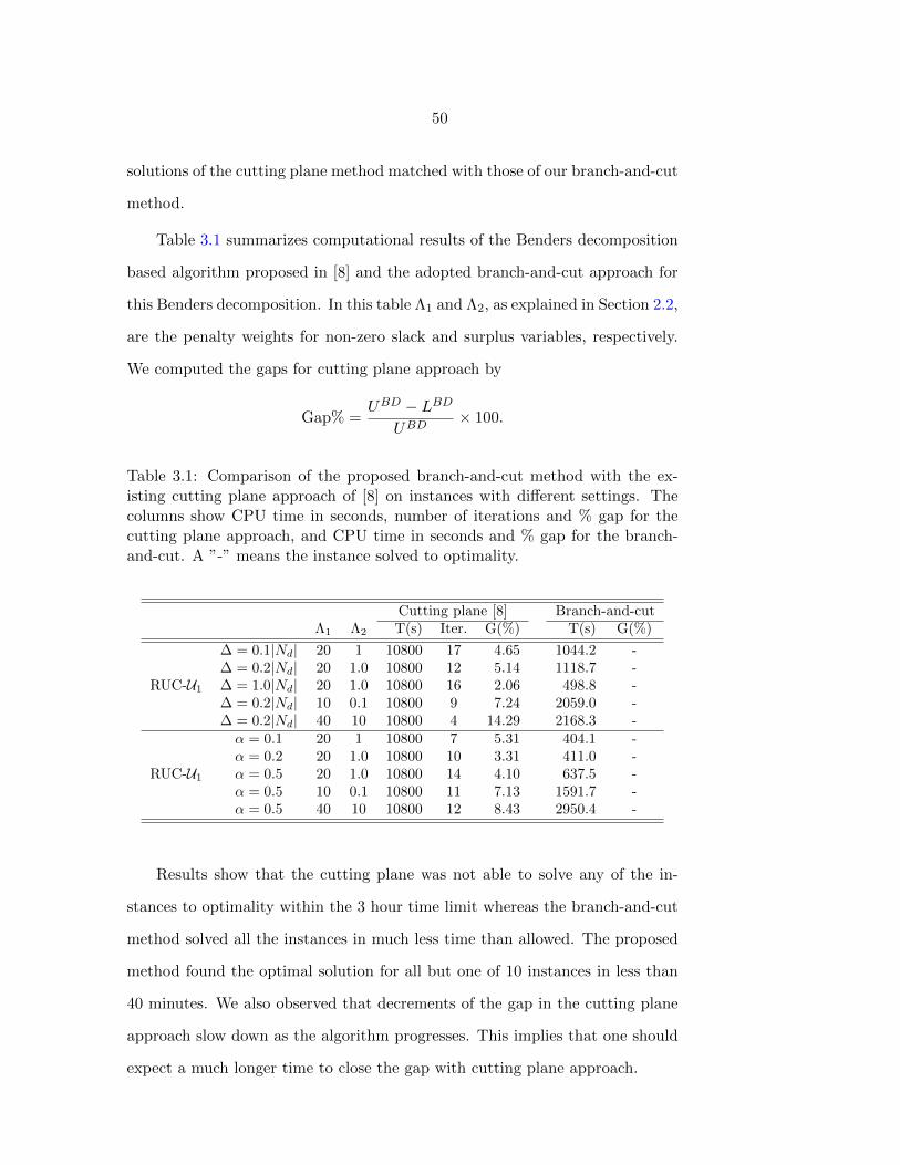
50

solutions of the cutting plane method matched with those of our branch-and-cut

method.

Table 3.1 summarizes computational results of the Benders decomposition

based algorithm proposed in [8] and the adopted branch-and-cut approach for

this Benders decomposition. In this table Λ1 and Λ2, as explained in Section 2.2,

are the penalty weights for non-zero slack and surplus variables, respectively.

We computed the gaps for cutting plane approach by

Gap% =UBD − LBD

UBD× 100.

Table 3.1: Comparison of the proposed branch-and-cut method with the ex-isting cutting plane approach of [8] on instances with different settings. Thecolumns show CPU time in seconds, number of iterations and % gap for thecutting plane approach, and CPU time in seconds and % gap for the branch-and-cut. A ”-” means the instance solved to optimality.

Cutting plane [8] Branch-and-cutΛ1 Λ2 T(s) Iter. G(%) T(s) G(%)

RUC-U1

∆ = 0.1|Nd| 20 1 10800 17 4.65 1044.2 -∆ = 0.2|Nd| 20 1.0 10800 12 5.14 1118.7 -∆ = 1.0|Nd| 20 1.0 10800 16 2.06 498.8 -∆ = 0.2|Nd| 10 0.1 10800 9 7.24 2059.0 -∆ = 0.2|Nd| 40 10 10800 4 14.29 2168.3 -

RUC-U1

α = 0.1 20 1 10800 7 5.31 404.1 -α = 0.2 20 1.0 10800 10 3.31 411.0 -α = 0.5 20 1.0 10800 14 4.10 637.5 -α = 0.5 10 0.1 10800 11 7.13 1591.7 -α = 0.5 40 10 10800 12 8.43 2950.4 -

Results show that the cutting plane was not able to solve any of the in-

stances to optimality within the 3 hour time limit whereas the branch-and-cut

method solved all the instances in much less time than allowed. The proposed

method found the optimal solution for all but one of 10 instances in less than

40 minutes. We also observed that decrements of the gap in the cutting plane

approach slow down as the algorithm progresses. This implies that one should

expect a much longer time to close the gap with cutting plane approach.

51

3.6 Conclusions

In this chapter, we adopted a branch-and-cut approach to solve the Ben-

ders decomposition algorithm for a robust optimization formulation of the unit

commitment problem. Being able to solve this problem in short amount of time

in a daily basis is one of the challenges of system operators.

The drawback of the existing algorithm is that it requires solving a mixed-

integer programming (MIP) problem in each iteration while this problem be-

comes larger during the course of the algorithm. As solving a MIP is compu-

tationally hard, this approach typically does not converge even for small sized

instances, hence cannot be a good option for solving real-world problems.

The adopted branch-and-cut scheme overcomes this drawback by solving

only one branch-and-bound tree and dynamically adding linear inequalities to

eliminate infeasible solutions and refine the feasible region within that branch-

and-bound procedure. The proposed approach dramatically improves the solu-

tion time for the instance that we considered. As a future step, we intend to

conduct testing on other instances including those with larger numbers of buses

and generators. In this way, we will ensure the method is robust and reliable.

Another possible test plan of the method is to compare the results of the

idea presented in Algorithm 4 with that proposed by Bertsimas et al. [8] on

the more efficient integer mixed-integer formulation presented in [39].

52

CHAPTER 4. AN APPROXIMATION FOR CVAR OF

ELECTRIC POWER PRODUCTION COST CONSIDERING

GENERATING UNIT FAILURES

4.1 Introduction

Reliability is a primary concern in power grid operations. Unexpected out-

ages of power grid elements, such as transmission lines and generators, can

result in dramatic electricity shortage. Uncertain outages of equipments, like

other uncertain parameters in power grid operations, were traditionally man-

aged by considering operating reserve requirements [68]. Alternate approaches

that allow the explicit modeling of the sources of uncertainty include stochastic

programming [55] and robust optimization [5, 60, 72]. Distributionally robust

optimization (DRO) is a moderately data-driven approach in which the true

distribution of a random variable is unknown and assumed to lie within a confi-

dence set. An example of applying the DRO framework for the unit commitment

problem with supply uncertainty considering random outages can be found in

[23].

Uncertain failures may include extremely rare events which lead to very

costly decisions. This concern can be addressed by considering and evaluating

the risk associated with the solutions. Imposing risk measures is a common

way to incorporate risk-averse preferences in the decisions. Several different

risk measures have been used in the literature. Considering expected value

and variance of the total profit or a certain quantity associated with a set of

UC decisions is a basic idea of managing risk. However, the most widely used

53

risk measure is Loss of Load Probability (LOLP) which can be formulated in

terms of chance constraints. These constraints enforce a requirement that the

probability that the total dispatch subject to random outages is greater than or

equal to the random net load/demand at that time period. To ensure system

reliability, constraints restricting this risk measure for all time periods based

on a specified confidence level are added to the problem. Some examples of

using chance constraints assuming the presence of random outages are [70, 71]

in which uncertain wind power and demand are considered, and [10, 14] which

consider probabilistic reserve criterion. Chance constraints restricting LOLP

are equivalent to restricting the Value at Risk (VaR) of the random loss of

load associated with a specified upper tail probability. However, VaR is not a

coherent risk measure as it does not satisfy the subadditivity property for gen-

eral probability distributions. Instead, another risk measure, Conditional Value

at Risk (CVaR), is more favored, because it is coherent and computationally

tractable [50, 51]. An example of using CVaR to formulate an optimization

model with random outages is [47] in which wind and demand uncertainty are

assumed.

Considering uncertain outages of power grid elements involves a large num-

ber of scenarios, for each of which a binary variable needs to be introduced, with

0 and 1 representing if a scenario will be selected or not. Some studies consider

all possible component failure scenarios such as [5, 55, 60, 72]. However, enu-

meration of a large set of failure scenarios requires significant computational

effort. Hence, most papers addressing this issue enumerate a given set of com-

ponents as candidates for possible failures [10, 26, 68]. Besides a large number

of binary variables indicating random outages, models considering chance con-

straints also contain additional binary variables to formulate this risk measure.

This makes these models computationally difficult even with a limited number

of scenarios. Therefore, in addition to methods considering a set of possible

outages (e.g., [10]), other approximation methods using exponential functions

54

(e.g., [14]) or Sample Average Approximation (e.g., [70, 71]) have been also

used for chance-constrained models.

Different solution algorithms such as Benders decomposition [68] and primal

and dual decomposition [72] have been used for models considering uncertain

outages of power grid components. Some other solution algorithms including

meta heuristic algorithms have been also used to mitigate the computational

difficulty of such problems. For example, a genetic algorithm is proposed to

find a feasible status of units in order to reduce the risk of unavailability of the

committed units and simultaneously satisfy several constraints such as ramp

rate, minimum up and down time [29]. Another genetic algorithm framework is

presented in [48] for a model with different sources of uncertainties such as load,

wind and solar generation and generator outages. An evolutionary algorithms

is used in [22] to solve power generating unit commitment problems with prob-

abilistic unit outages. Finally, a particle swarm optimization is developed to

locate the optimum generation combination for a UC model considering gener-

ator outages, where the reliability requirement is incorporated into the spinning

reserve constraint [69].

Because considering random outages in power systems operations involves

enumeration of a large set of possible failure scenarios and, therefore, requires

additional computational effort, much research has been done to find more

efficient formulations and solution procedures. However, it is crucial to be

able to analyze the reliability of power systems in a reasonable time period.

Hence, it is worth investigating approximation approaches that do not require

enumeration of all or a set of possible failure scenarios.

The aim of this chapter is to present an efficient and time-saving approach

for evaluating the risk associated with the power system. Among different risk

measures, CVaR is attractive because it is coherent and also provides informa-

tion about the related VaR and LOLP because of the CVaR is defined upon

VaR [50, 51]. However, it is difficult to compute CVaR by solving a stochas-

55

tic program along with the huge number of scenarios that would be added to

address contingencies. Generally, it takes more scenarios to estimate CVaR,

because it deals with the tail of the distribution. An alternative approach is

to apply a renewal reward process to asymptotically approximate CVaR as was

done to approximate cost variance [56].

In this study, we estimate the CVaR of electric power production cost over

a specified time. Assuming a given set of committed units, under simplifying

assumptions, we apply a renewal reward process, an asymptotic central limit

theorem and the definition of CVaR for the normal distribution to achieve this

approximation. In probability theory, a renewal process is a counting process

for which the times between successive events are independent and identically

distributed with an arbitrary distribution [52]. Let N(t), t ≥ 0, be a count-

ing process and let Xn denote the time between the (n − 1)st and the nth

event of this process, n ≥ 1. If the sequence of nonnegative random variables

X1, X2, . . . is independent and identically distributed, then the counting pro-

cess N(t), t ≥ 0, is a renewal process. If we denote a random reward earned at

the time of the nth renewal by Rn, then the total reward earned by time t is

represented by

R(t) =

N(t)∑n=1

Rn.

Assume that Γ(t) represents the total reward up to time t experienced by

a renewal process with interrenewal time T and reward per renewal Z. Smith

[59] showed that the cumulative reward is asymptotically normal and Brown

and Solomon [11] showed that the variance of Γ(t) is given by

56

V ar[Γ(t)] = at+ b+ o(1)

where

a = τ2θ21/τ

31 − 2η11θ1/τ

21 + θ2/τ1,

and

τ1 = E(T ), τ2 = E(T 2), θ1 = E(Z), θ2 = E(Z2), η11 = E(ZT ).

This justifies the use of normal formulations to compute the CVaR of the

cost in this study.

Many applications of renewal theory involve costs which can be simply seen

as a negative reward. In the next section, we explain the application of this

theory in asymptotically approximating of the variance of the cost of electric

power system with random failure and repair times for the generating units.

4.2 Problem Statement

Security of a power system refers to its ability to survive contingencies,

while avoiding any undesirable disruption of service. The concept of N-1 se-

curity assessment has been developed to quantify security. It is a standard

enforced by the North American Electric Reliability Corporation (NERC). In

this study, we consider the system to be in a N-1 secure state. In other words,

the system is able to operate with one component failure. The N-1 security

standard reflects the low probability that unscheduled outages of more than

one component would occur at the same time.

Assume that N generating units have been committed for a specified time

horizon. Unit i has capacity ci (in MW) and variable operating cost di (in

$/MW h), with d1 ≤ d2 ≤ · · · ≤ dN . The load on the system at any time is

satisfied by the least expensive set of units available, and, in case insufficient

capacity is available to satisfy the load, the cost of any unmet demand is given

57

by dN+1 > dN . Let Ai(s) be the operating state of unit i at time s, so that

Ai(s) = 1 if unit i is available and 0 otherwise. Assume that the operating

state of each unit follows a stationary continuous Markov chain with a failure

rate λi and repair rate µi per hour. The ratio pi = λi/(λi + µi) represents the

proportion of time during which unit i is not available.

In relation to the previous chapters, we are simplifying here by ignoring

ramping, minimum up and down-time, and transmission constraints. Therefore,

this approximation considers only failures of generating units. One major and

one minor simplifying assumption are also considered for the approximation.

First, at most one generating unit is unavailable at any point in time which

is consistent with the N-1 security criterion; Second, the times when failures

occur and units are returned to service coincide with the beginning of a load

cycle. By the first assumption, the state of the system, [A1(s), A2(s), . . . , AN (s)]

at time s, can be described as a renewal process. We suppose all units are

available at time 0, and after a random time, X, one unit fails. On basis of the

first assumption, no other failure occurs during this failure time, Y . The time

T = X + Y then represents the time when the failed unit is restored to service

and follows a renewal process. Denote the total production cost during T by

Z = U + V where U is the cost during X and V is the cost during Y . The

second assumption simplifies the estimation of the costs U and V .

According to the second assumption, the time to failure, X, consists of a

number, K, of load cycles plus a remainder, R. Assuming ∆ as the length of

each load cycle, we have: X = K∆ + R. Similarly, for a random unit J = j,

the unit down time can be written as Y = Kj∆ + Rj , where Kj and Rj have

distributions similar to K and R, respectively.

Ryan [56] developed formulas to compute the slope, a, of the asymptotic

variance. The intercept, b, is a function of moments up to the third order,

and will not be used. The expected production cost, E[Γ(t)], is approximated

as (θ1/τ1)t. We will use this µ as the expected value in future computations.

58

Variables X and Y are independent and follow exponential distributions with

rate Λ =∑

j λj and M , respectively, where M = µj with probability λj/Λ.

Considering J as the index of the unit that fails, we have J = j with probability

λj/Λ. Thus, the quantities τ1 and τ2 can be computed as follows.

τ1 = E(T ) = E(X) + E(Y ),

where

E(X) = 1/Λ,

and

E(Y ) = EJ [E(Y |J)] =∑j

λjµjΛ

.

τ2 = E(T 2) = E[(X + Y )2] = E(X2) + 2E(X)E(Y ) + E(Y 2),

where

E(X2) = 2/Λ,

and

E(Y 2) = EJ [E(Y 2|J)] =∑j

2λjµ2jΛ.

To evaluate the parameters involving Z = U + V note that U depends

on X, whereas V depends on Y . According to the second assumption, the

time to failure, X, can be written as X = K∆ + R where K has a geometric

distribution with parameter 1 − e−Λ∆, and R is distributed according to the

truncated exponential density function

f(r) = Λe−Λr/(1− e−Λ∆), for 0 < r < ∆.

Given J = j, the time to repair, Y , can be also written as Y = Kj∆ +Rj ,

where Kj and Rj have distributions similar to K and R, respectively, with Λ

replaced by µj .

59

Parameters θ1, θ2 and η11 which involve moments of Z can be computed

as listed below. We refer to [56] for more details on these formulations.

θ1 = E(Z) = E(U) + E(V ).

θ2 = E(Z2) = V ar(Z) + [E(Z)]2,

where

V ar(Z) = V ar(U) + V ar(V )

and

V ar(U) =E +X[V ar(U |X)] + V arX [E(U |X)]

V ar(V ) =EJ [V ar(V |J)] + V arJ [E(V |J)].

The conditional values are computed as

EJ [V ar(V |J)] =∑j

λjΛ

V ar(KJ)

∆∫0

vJ(t)dt

2

+ V ar

Rj∫0

v(t)dt

V arJ [E(V |J)] =∑j

λjΛ

[E(V |J = j)]2 −

∑j

λjΛE(V |J = j)

2

,

E [V |J = j] =E[Kj ]

∆∫0

vj(t)dt+ E

Rj∫0

vj(t)dt

.Finally,

η11 = E(ZT ) = E(UX) + E(V )E(X) + E(U)E(Y ) + E(V Y ).

Here, u(s) is the production cost at time s with all units available, vj(s)

is the cost at time s with unit j unavailable, and Λ is the parameter of the

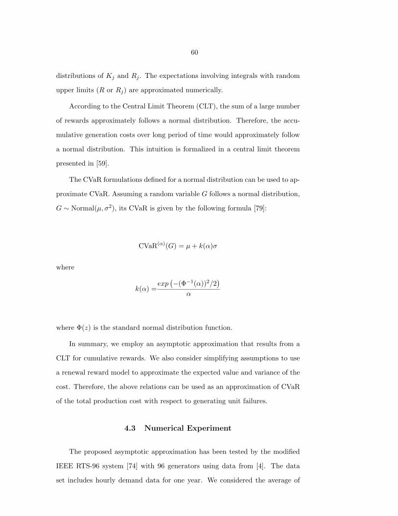
60

distributions of Kj and Rj . The expectations involving integrals with random

upper limits (R or Rj) are approximated numerically.

According to the Central Limit Theorem (CLT), the sum of a large number

of rewards approximately follows a normal distribution. Therefore, the accu-

mulative generation costs over long period of time would approximately follow

a normal distribution. This intuition is formalized in a central limit theorem

presented in [59].

The CVaR formulations defined for a normal distribution can be used to ap-

proximate CVaR. Assuming a random variable G follows a normal distribution,

G ∼ Normal(µ, σ2), its CVaR is given by the following formula [79]:

CVaR(α)(G) = µ+ k(α)σ

where

k(α) =exp

(−(Φ−1(α))2/2

)α

where Φ(z) is the standard normal distribution function.

In summary, we employ an asymptotic approximation that results from a

CLT for cumulative rewards. We also consider simplifying assumptions to use

a renewal reward model to approximate the expected value and variance of the

cost. Therefore, the above relations can be used as an approximation of CVaR

of the total production cost with respect to generating unit failures.

4.3 Numerical Experiment

The proposed asymptotic approximation has been tested by the modified

IEEE RTS-96 system [74] with 96 generators using data from [4]. The data

set includes hourly demand data for one year. We considered the average of

61

load scenarios for each hour in a day over the whole year, and set the sum of

loads over all buses as the total load for each hour. The production cost is

considered as the average of stepwise production costs for each generators, and

the cost of unmet demand is considered as 100 $/MWh. There are 19 wind farms

accommodated to the grid as in [44] with wind scenarios extracted from the

NREL wind data sets [3]. We selected 19 renewable generation data randomly

from this data set and computed net load for each hour as the difference between

load and the output of renewable generation.

We tested a subset of generators which are committed based on the solution

from optimization problem without constraints on ramping, minimum up and

down-time, and transmission lines. This set consists of 47 generators out of 96

generators. Tables 4.1 and 4.2 contains generating unit data and sequence of

load levels for this example respectively.

In order to evaluate the quality of the proposed asymptotic approximation,

we compared the approximated results with the results from simulation. Our

approach is to simulate outages and dispatch over all hours in the horizon

and compute cumulative costs over the horizon and calculate CVaR of the

cost directly from simulated costs. Algorithm 5 shows the pseudocode for the

simulation of CVaR of the cost. In implementing the simulation, we consider

bigreps = 1000 and reps = 100.

In the pseudocode presented in Algorithm 5, when we simulated the FailedUnits

array, we calculated the cost of satisfying the required loads in each hour

given the failed units of the associated hour. Note that when an entry in

the FailedUnits array is 0, it implies that all units are available. We insert 0

for the time that the next failure time is generated, because we assumed that

in each period at most one unit could fail. Hence, until the next failure time

there will be no failed units. Once we have the cost for all reps inner loops, we

can calculate the VaR and CVaR for 95th percentile of each outer loop with

given relations for VaR and CVaR.

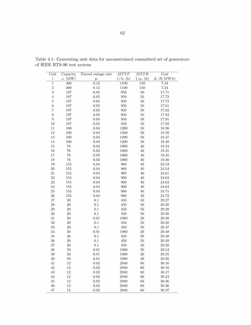
62

Table 4.1: Generating unit data for unconstrained committed set of generatorsof IEEE RTS-96 test system

Unit Capacity Forced outage rate MTTF MTTR Costi ci (MW) pi 1/λi (h) 1/µi (h) di ($/MWh)

1 400 0.12 1100 150 7.332 400 0.12 1100 150 7.343 197 0.05 950 50 17.714 197 0.05 950 50 17.725 197 0.05 950 50 17.736 197 0.05 950 50 17.817 197 0.05 950 50 17.828 197 0.05 950 50 17.839 197 0.05 950 50 17.9110 197 0.05 950 50 17.9211 100 0.04 1200 50 18.3812 100 0.04 1200 50 18.3913 100 0.04 1200 50 18.4714 100 0.04 1200 50 18.4815 76 0.02 1960 40 19.3416 76 0.02 1960 40 19.3517 76 0.02 1960 40 19.4518 76 0.02 1960 40 19.4619 155 0.04 960 40 24.5320 155 0.04 960 40 24.5421 155 0.04 960 40 24.6122 155 0.04 960 40 24.6223 155 0.04 960 40 24.6324 155 0.04 960 40 24.6425 155 0.04 960 40 24.7126 155 0.04 960 40 24.7227 20 0.1 450 50 29.2728 20 0.1 450 50 29.2829 20 0.1 450 50 29.2930 20 0.1 450 50 29.3031 50 0.01 1980 20 29.3832 20 0.1 450 50 29.3833 20 0.1 450 50 29.4734 50 0.01 1980 20 29.4835 20 0.1 450 50 29.4836 20 0.1 450 50 29.4937 20 0.1 450 50 29.5038 50 0.01 1980 20 29.5439 50 0.01 1980 20 29.5540 50 0.01 1980 20 29.5641 12 0.02 2940 60 30.1642 12 0.02 2940 60 30.1643 12 0.02 2940 60 30.1744 12 0.02 2940 60 30.2445 12 0.02 2940 60 30.3646 12 0.02 2940 60 30.3647 12 0.02 2940 60 30.37

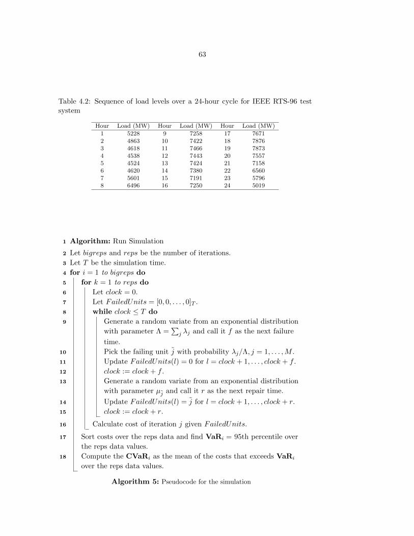
63

Table 4.2: Sequence of load levels over a 24-hour cycle for IEEE RTS-96 testsystem

Hour Load (MW) Hour Load (MW) Hour Load (MW)

1 5228 9 7258 17 76712 4863 10 7422 18 78763 4618 11 7466 19 78734 4538 12 7443 20 75575 4524 13 7424 21 71586 4620 14 7380 22 65607 5601 15 7191 23 57968 6496 16 7250 24 5019

1 Algorithm: Run Simulation

2 Let bigreps and reps be the number of iterations.

3 Let T be the simulation time.

4 for i = 1 to bigreps do

5 for k = 1 to reps do

6 Let clock = 0.

7 Let FailedUnits = [0, 0, . . . , 0]T .

8 while clock ≤ T do

9 Generate a random variate from an exponential distribution

with parameter Λ =∑

j λj and call it f as the next failure

time.

10 Pick the failing unit j with probability λj/Λ, j = 1, . . . ,M .

11 Update FailedUnits(l) = 0 for l = clock + 1, . . . , clock + f .

12 clock := clock + f .

13 Generate a random variate from an exponential distribution

with parameter µj and call it r as the next repair time.

14 Update FailedUnits(l) = j for l = clock + 1, . . . , clock + r.

15 clock := clock + r.

16 Calculate cost of iteration j given FailedUnits.

17 Sort costs over the reps data and find VaRi = 95th percentile over

the reps data values.

18 Compute the CVaRi as the mean of the costs that exceeds VaRi

over the reps data values.

Algorithm 5: Pseudocode for the simulation

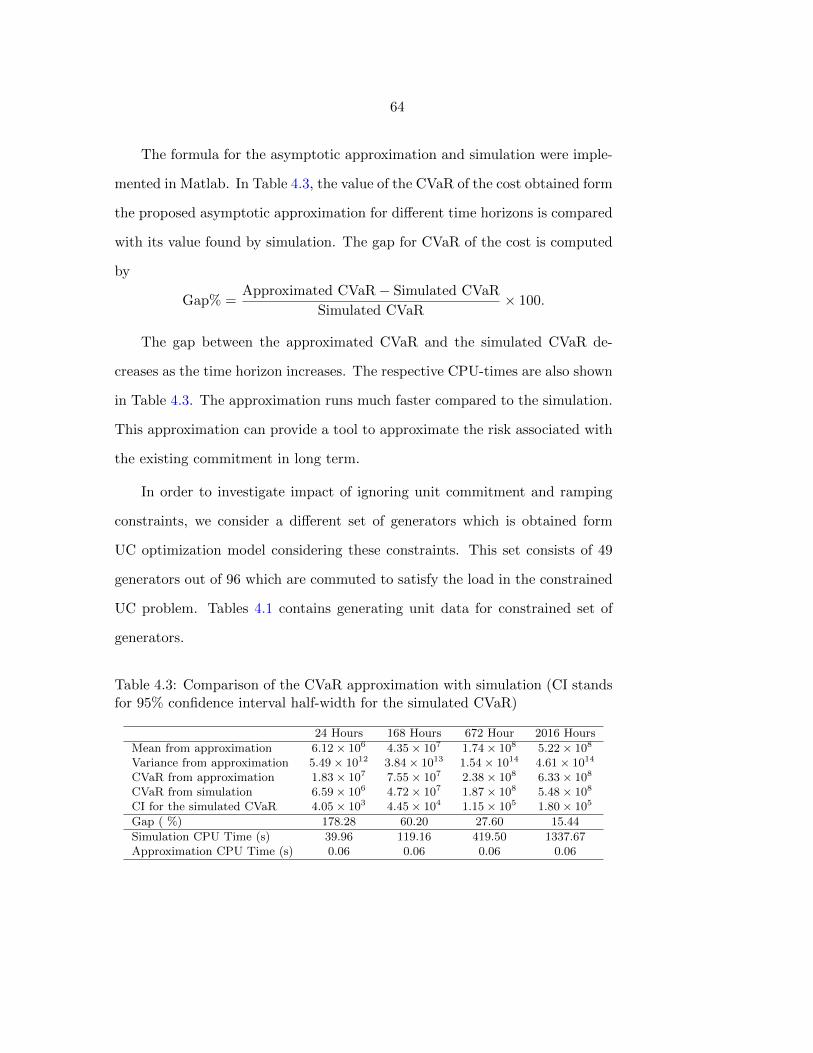
64

The formula for the asymptotic approximation and simulation were imple-

mented in Matlab. In Table 4.3, the value of the CVaR of the cost obtained form

the proposed asymptotic approximation for different time horizons is compared

with its value found by simulation. The gap for CVaR of the cost is computed

by

Gap% =Approximated CVaR− Simulated CVaR

Simulated CVaR× 100.

The gap between the approximated CVaR and the simulated CVaR de-

creases as the time horizon increases. The respective CPU-times are also shown

in Table 4.3. The approximation runs much faster compared to the simulation.

This approximation can provide a tool to approximate the risk associated with

the existing commitment in long term.

In order to investigate impact of ignoring unit commitment and ramping

constraints, we consider a different set of generators which is obtained form

UC optimization model considering these constraints. This set consists of 49

generators out of 96 which are commuted to satisfy the load in the constrained

UC problem. Tables 4.1 contains generating unit data for constrained set of

generators.

Table 4.3: Comparison of the CVaR approximation with simulation (CI standsfor 95% confidence interval half-width for the simulated CVaR)

24 Hours 168 Hours 672 Hour 2016 Hours

Mean from approximation 6.12× 106 4.35× 107 1.74× 108 5.22× 108

Variance from approximation 5.49× 1012 3.84× 1013 1.54× 1014 4.61× 1014

CVaR from approximation 1.83× 107 7.55× 107 2.38× 108 6.33× 108

CVaR from simulation 6.59× 106 4.72× 107 1.87× 108 5.48× 108

CI for the simulated CVaR 4.05× 103 4.45× 104 1.15× 105 1.80× 105

Gap ( %) 178.28 60.20 27.60 15.44

Simulation CPU Time (s) 39.96 119.16 419.50 1337.67Approximation CPU Time (s) 0.06 0.06 0.06 0.06

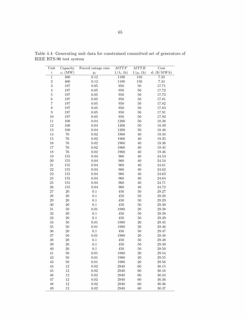
65

Table 4.4: Generating unit data for constrained committed set of generators ofIEEE RTS-96 test system

Unit Capacity Forced outage rate MTTF MTTR Costi ci (MW) pi 1/λi (h) 1/µi (h) di ($/MWh)

1 400 0.12 1100 150 7.332 400 0.12 1100 150 7.343 197 0.05 950 50 17.714 197 0.05 950 50 17.725 197 0.05 950 50 17.736 197 0.05 950 50 17.817 197 0.05 950 50 17.828 197 0.05 950 50 17.839 197 0.05 950 50 17.9110 197 0.05 950 50 17.9211 100 0.04 1200 50 18.3812 100 0.04 1200 50 18.3913 100 0.04 1200 50 18.4814 76 0.02 1960 40 19.3415 76 0.02 1960 40 19.3516 76 0.02 1960 40 19.3617 76 0.02 1960 40 19.4518 76 0.02 1960 40 19.4619 155 0.04 960 40 24.5320 155 0.04 960 40 24.5421 155 0.04 960 40 24.6122 155 0.04 960 40 24.6223 155 0.04 960 40 24.6324 155 0.04 960 40 24.6425 155 0.04 960 40 24.7126 155 0.04 960 40 24.7227 20 0.1 450 50 29.2728 20 0.1 450 50 29.2829 20 0.1 450 50 29.2930 20 0.1 450 50 29.3031 50 0.01 1980 20 29.3832 20 0.1 450 50 29.3833 20 0.1 450 50 29.3934 50 0.01 1980 20 29.4535 50 0.01 1980 20 29.4636 20 0.1 450 50 29.4737 50 0.01 1980 20 29.4838 20 0.1 450 50 29.4839 20 0.1 450 50 29.4940 20 0.1 450 50 29.5041 50 0.01 1980 20 29.5442 50 0.01 1980 20 29.5543 50 0.01 1980 20 29.5644 12 0.02 2940 60 30.1545 12 0.02 2940 60 30.1646 12 0.02 2940 60 30.2447 12 0.02 2940 60 30.3648 12 0.02 2940 60 30.3649 12 0.02 2940 60 30.37

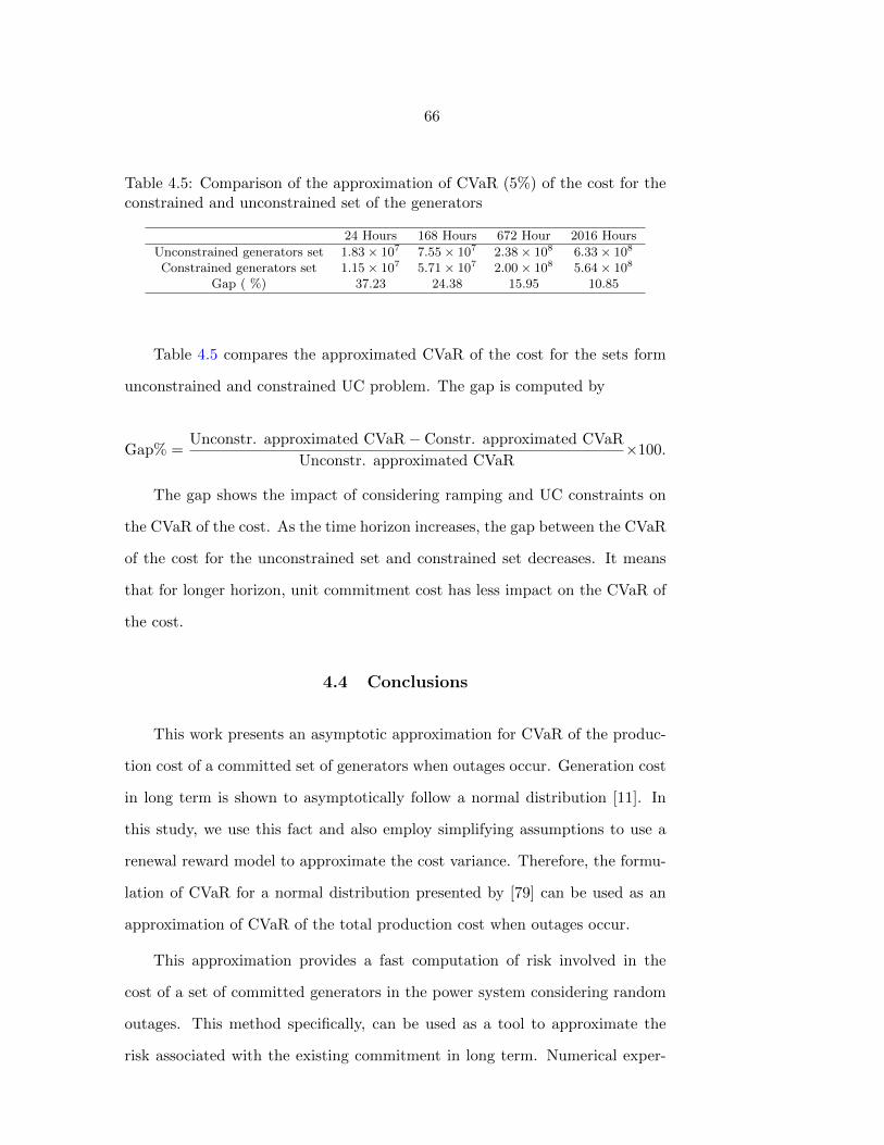
66

Table 4.5: Comparison of the approximation of CVaR (5%) of the cost for theconstrained and unconstrained set of the generators

24 Hours 168 Hours 672 Hour 2016 Hours

Unconstrained generators set 1.83× 107 7.55× 107 2.38× 108 6.33× 108

Constrained generators set 1.15× 107 5.71× 107 2.00× 108 5.64× 108

Gap ( %) 37.23 24.38 15.95 10.85

Table 4.5 compares the approximated CVaR of the cost for the sets form

unconstrained and constrained UC problem. The gap is computed by

Gap% =Unconstr. approximated CVaR− Constr. approximated CVaR

Unconstr. approximated CVaR×100.

The gap shows the impact of considering ramping and UC constraints on

the CVaR of the cost. As the time horizon increases, the gap between the CVaR

of the cost for the unconstrained set and constrained set decreases. It means

that for longer horizon, unit commitment cost has less impact on the CVaR of

the cost.

4.4 Conclusions

This work presents an asymptotic approximation for CVaR of the produc-

tion cost of a committed set of generators when outages occur. Generation cost

in long term is shown to asymptotically follow a normal distribution [11]. In

this study, we use this fact and also employ simplifying assumptions to use a

renewal reward model to approximate the cost variance. Therefore, the formu-

lation of CVaR for a normal distribution presented by [79] can be used as an

approximation of CVaR of the total production cost when outages occur.

This approximation provides a fast computation of risk involved in the

cost of a set of committed generators in the power system considering random

outages. This method specifically, can be used as a tool to approximate the

risk associated with the existing commitment in long term. Numerical exper-

67

iments and the comparison with simulation results shows the precision of the

asymptotic approximation. We also show that as the time horizon increases, the

impact of ignoring unit commitment and ramping constraints on approximation

of the CVaR of the cost is less.

68

CHAPTER 5. GENERAL CONCLUSION

The dissertation is a combination of three papers that address the con-

sideration of risk in the unit commitment problem under supply and demand

uncertainty. The topics include approaches to consider risk in unit commitment

problem and methodologies to solve them.

Chapter 2 studies and compares two formulations based on two different

approaches to deal with net load uncertainty in unit commitment problem; two-

stage stochastic programming and robust optimization. A two-stage stochastic

unit commitment problem is formulated with an objective function that includes

CVaR of the dispatch costs. The robust optimization approach is considered

with two different definition of uncertainty set. The first one, which is frequently

used in the literature, is defined by a lower bound and an upper bound with a

parameter controlling the deviation. We also applied another uncertainty set

which is defined as a combination of historical scenarios.

The goal of this chapter is to study stochastic programming and robust op-

timization as the most widely used approaches in the unit commitment problem

under net load uncertainty in order to compare the solutions and evaluate the

effectiveness of these approaches. Numerical results show that stochastic pro-

gramming formulation incorporating CVaR can achieve the most efficient com-

binations of cost and risk. Between the two uncertainty set formulations for

robust optimization, the data-driven method results in better cost-risk trade-

offs than the uncertainty set based on ranges.

69

In chapter 3, we enhanced the existing algorithm to solve robust optimiza-

tion formulation by implementing a branch-and-cut algorithm. The drawback

of the existing algorithm is that it requires the solution of a mixed-integer pro-

gramming (MIP) problem in each iteration while this problem becomes larger

during the course of the algorithm. As solving a MIP is computationally hard,

this approach typically does not converge even for small sized problems and,

hence, cannot be a good option for ISOs to deal with real-world problems.

The adopted branch-and-cut scheme overcomes this issue by solving only

one single branch-and-bound tree and dynamically adding linear inequalities to

eliminate infeasible solutions and refine the feasible region within that branch-

and-bound. The proposed approach dramatically improves the solution time

for RUC.

In chapter 4, we developed an asymptotic approximation to estimate CVaR

of electric power production cost considering random outages of generating

units. Considering simplifying assumptions, we apply a renewal reward process

and definition of CVaR for normal distribution to achieve this approximation.

Most studies considering outages in the UC problem enumerate a given

set of components as candidates for possible failures or consider all possible

component failure scenarios which requires a lot of computational effort. Our

approximation provides a fast computation for this situation. The numerical

experiments and comparison with simulation results evaluate the precision of

the asymptotic approximation for CVaR of the cost. The approximation gives

more accurate solutions as it runs for a longer time horizon. This method can

provide a tool to approximate the risk associated with generating unit failures

given an existing commitment in long term operation.

Although the dissertation has reached its aims, there were some limitations

which might be considered in future research. Chapter 2 focuses on stochastic

programming and robust optimization. Other approaches of considering risk

70

such as chance constraints could be evaluated. Chapter 3 shows the efficiency of

the proposed branch and cut method; however, this method could be evaluated

by other test cases. It can also be implemented on alternative formulations of

the UC which might be more efficient. In Chapter 4, ramping, minimum up

and down-time, and transmission constraints are ignored. This simplification

might affect the approximation results. The approximation could be extended

to incorporate previously-decided commitments for each hour. In addition, it

was assumed that no more than one generator can be failed at a time. However,

considering more than one failure can be another future research topic.

71

BIBLIOGRAPHY

[1] 20% Wind Energy by 2030: Increasing the best Wind Energy’s Contribution

to U.S. Electricity Supply. http://www.nrel.gov/docs/fy08osti/41869.

pdf.

[2] California ISO. www.caiso.com.

[3] NREL Eastern Wind Dataset. http://www.nrel.gov/electricity/

transmission/eastern_wind_methodology.html.

[4] Renewable Energy Analysis Laboratory, Department of Electrical En-

gineering, University of Washington. http://www2.ee.washington.edu/

research/real/library.html.

[5] An, Y. and Zeng, B. (2015). Exploring the modeling capacity of two-stage

robust optimization: Variants of robust unit commitment model. Power

Systems, IEEE Transactions on, 30(1):109–122.

[6] Asensio, M. and Contreras, J. (2016). Stochastic unit commitment in iso-

lated systems with renewable penetration under cvar assessment. IEEE

Transactions on Smart Grid, 7(3):1356–1367.

[7] Bertsimas, D. and Brown, D. B. (2009). Constructing uncertainty sets for

robust linear optimization. Operations Research, 57:1483–1495.

[8] Bertsimas, D., Litvinov, E., Sun, X. A., Zhao, J., and Zheng, T. (2013).

Adoptive robust optimization for the security constrained unit commitment

problem. IEEE Transaction on Power Systems, 28:52–63.

72

[9] Bouffard, F., Galiana, F., and Conejo, A. (2005). Market-clearing with

stochastic security-part i: formulation. Power Systems, IEEE Transactions

on, 20(4):1818–1826.

[10] Bouffard, F. and Galiana, F. D. (2004). An electricity market with a prob-

abilistic spinning reserve criterion. IEEE Transactions on Power Systems,

19(1):300–307.

[11] Brown, M. and Solomon, H. (1975). A second-order approximation for

the variance of a renewal reward process. Stochastic Processes and their

Applications, 3(3):301 – 314.

[12] Bukhsh, W., Papakonstantinou, A., and Pinson, P. A robust optimisa-

tion approach using cvar for unit commitment in a market with probabilistic

offers. http://pierrepinson.com/docs/Bukhshetal2016.pdf.

[13] Carrion, M. and Arroyo, J. M. (2006). A computationally efficient mixed-

integer linear formulation for the thermal unit commitment problem. IEEE

Transaction on Power Systems, 21:1371–1378.

[14] Chattopadhyay, D. and Baldick, R. (2002). Unit commitment with proba-

bilistic reserve. In Power Engineering Society Winter Meeting, 2002. IEEE,

volume 1, pages 280–285. IEEE.

[15] Cheung, K., Gade, D., Silva-Monroy, C., Ryan, S. M., Watson, J.-P., Wets,

R. J.-B., and Woodruff, D. L. (2015). Toward scalable stochastic unit com-

mitment. part 2: Solver configuration and performance assessment. Energy

Systems, 6(3):417–438.

[16] Dai, C., Wu, L., and Wu, H. (2016). A multi-band uncertainty set based

robust scuc with spatial and temporal budget constraints. Power Systems,

IEEE Transactions on. doi:10.1109/TPWRS.2016.2525009.

73

[17] Duran, M. A. and Grossmann, I. E. (1986). An outer-approximation al-

gorithm for a class of mixed-integer nonlinear programs. Mathematical Pro-

gramming, 36(3):307–339.

[18] Dvorkin, Y., Pandzic, H., Ortega-Vazquez, M. A., and Kirschen, D. S.

(2015). A hybrid stochastic/interval approach to transmission-constrained

unit commitment. Power Systems, IEEE Transactions on, 30(2):621–631.

[19] Feng, Y., Rios, I., Ryan, S. M., Spurkel, K., Watson, J.-P., Wets, R. J.-B.,

and Woodruff, D. L. (2015). Toward scalable stochastic unit commitment.

part 1: load scenario generation. Energy Systems, 6(3):309–329.

[20] Feng, Y. and Ryan, S. M. (2016). Solution sensitivity-based scenario reduc-

tion for stochastic unit commitment. Computational Management Science,

13(1):29–62.

[21] Fletcher, R. and Leyffer, S. (1994). Solving mixed integer nonlinear pro-

grams by outer approximation. Mathematical Programming, 66(1):327–349.

[22] Georgopoulou, C. A. and Giannakoglou, K. C. (2010). Metamodel-assisted

evolutionary algorithms for the unit commitment problem with probabilistic

outages. Applied Energy, 87(5):1782–1792.

[23] Gourtani, A., Xu, H., Pozo, D., and Nguyen, T.-D. (2016). Robust unit

commitment with n-1 security criteria. Mathematical Methods of Operations

Research, 83(3):373–408.

[24] Guan, Y. and Wang, J. (2014). Uncertainty sets for robust unit commit-

ment. Power Systems, IEEE Transactions on, 29(3):1439–1440.

[25] Hamzeei, M. and Luedtke, J. (2014). Linearization-based algorithms for

mixed-integer nonlinear programs with convex continuous relaxation. Journal

of Global Optimization, 59:343–365.

74

[26] Hedman, K. W., Ferris, M. C., O’Neill, R. P., Fisher, E. B., and Oren,

S. S. (2010). Co-optimization of generation unit commitment and transmis-

sion switching with n-1 reliability. IEEE Transactions on Power Systems,

25(2):1052–1063.

[27] Heitsch, H. and Rmisch, W. (2003). Scenario reduction algorithms in

stochastic programming. Computational Optimization and Applications,

24(2-3):187–206.

[28] Huang, Y., Zheng, Q. P., and Wang, J. (2014). Two-stage stochastic

unit commitment model including non-generation resources with conditional

value-at-risk constraints. Electric Power Systems Research, 116:427 – 438.

[29] Jha, R., Ghose, T., Sedimbi, D., and Lalitha, E. (2008). Solution of

unit commitment using modified genetic algorithm considering the effect of

unit outage uncertainty. International Journal of Power & Energy Systems,

28(1):1–8.

[30] Jiang, R., Wang, J., and Guan, Y. (2012). Robust unit commitment with

wind power and pumped storage hydro. Power Systems, IEEE Transactions

on, 27(2):800–810.

[31] Jiang, R., Wang, J., Zhang, M., and Guan, Y. (2013). Two-stage minimax

regret robust unit commitment. Power Systems, IEEE Transactions on,

28(3):2271–2282.

[32] Jiang, R., Zhang, M., Li, G., and Guan, Y. (2014). Two-stage network con-

strained robust unit commitment problem. European Journal of Operational

Research, 234(3):751 – 762.

[33] Lorca, A. and Sun, X. A. (2015). Adaptive robust optimization with dy-

namic uncertainty sets for multi-period economic dispatch under significant

wind. Power Systems, IEEE Transactions on, 30(4):1702–1713.

75

[34] Lorca, A., Sun, X. A., Litvinov, E., and Zheng, T. (2016). Multistage

adaptive robust optimization for the unit commitment problem. Operations

Research, 64(1):32–51.

[35] Martinez, G. and Anderson, L. (2014). Toward a scalable chance-

constrained formulation for unit commitment to manage high penetration

of variable generation. In Communication, Control, and Computing (Aller-

ton), 2014 52nd Annual Allerton Conference on, pages 723–730. IEEE.

[36] Martinez, G. and Anderson, L. (2015). A risk-averse optimization model for

unit commitment problems. In 2015 48th Hawaii International Conference,

pages 2577–2585. IEEE Computer Society.

[37] Matos, M. and Bessa, R. (2011). Setting the operating reserve using

probabilistic wind power forecasts. Power Systems, IEEE Transactions on,

26(2):594–603.

[38] Morales, J., Conejo, A., and Perez-Ruiz, J. (2009). Economic valuation

of reserves in power systems with high penetration of wind power. Power

Systems, IEEE Transactions on, 24(2):900–910.

[39] Morales-Espana, G., Latorre, J. M., and Ramos, A. (2013). Tight and

compact MILP formulation for the thermal unit commitment problem. Power

Systems, IEEE Transactions on, 28(4):4897–4908.

[40] Morales-Espana, G., Latorre, J. M., and Ramos, A. (2013). Tight and

compact milp formulation of start-up and shut-down ramping in unit com-

mitment. Power Systems, IEEE Transactions on, 28(2):1288–1296.

[41] Murillo-Snchez, C. E., Zimmerman, R. D., Anderson, C. L., and Thomas,

R. J. (2013). A stochastic, contingency-based security-constrained optimal

power flow for the procurement of energy and distributed reserve. Decision

Support Systems, 56(0):1 – 10.

76

[42] Naoum-Sawaya, J. and Elhedhli, S. (2013). An interior-point benders based

branch-and-cut algorithm for mixed integer programs. Annals of Operations

Research, 210(1):33–55.

[43] Ozturk, U., Mazumdar, M., and Norman, B. (2004). A solution to the

stochastic unit commitment problem using chance constrained programming.

Power Systems, IEEE Transactions on, 19(3):1589–1598.

[44] Pandzic, H., Dvorkin, Y., Qiu, T., Wang, Y., and Kirschen, D. S. (2016).

Toward cost-efficient and reliable unit commitment under uncertainty. IEEE

Transactions on Power Systems, 31(2):970–982.

[45] Pandzic, H., Qiu, T., and Kirschen, D. S. (2013). Comparison of state-of-

the-art transmission constrained unit commitment formulations. In Power

and Energy Society General Meeting (PES), 2013 IEEE, pages 1–5. IEEE.

[46] Peralta, J., Perez-Ruiz, J., and de la Torre, S. (2013). Unit commitment

with load uncertainty by joint chance-constrained programming. In Pow-

erTech (POWERTECH), 2013 IEEE Grenoble, pages 1–6.

[47] Pozo, D. and Contreras, J. (2013). A chance-constrained unit commitment

with an security criterion and significant wind generation. IEEE Transactions

on Power Systems, 28(3):2842–2851.

[48] Quan, H., Srinivasan, D., Khambadkone, A. M., and Khosravi, A. (2015).

A computational framework for uncertainty integration in stochastic unit

commitment with intermittent renewable energy sources. Applied Energy,

152:71–82.

[49] Rei, W., Cordeau, J.-F., Gendreau, M., and Soriano, P. (2009). Accel-

erating benders decomposition by local branching. INFORMS Journal on

Computing, 21(2):333–345.

77

[50] Rockafellar, R. T. and Uryasev, S. (2002). Conditional value-at-risk for

general loss distributions. J. of Banking and Fincance, 26:1443–1471.

[51] Rockafellar, R. T. and Uryasev, S. (2006). Optimization of conditional

value-at-risk. J. Risk, 2:21–41.

[52] Ross, S. M. (2010). Introduction to Probability Models. 10th Edition.

Academic Press.

[53] Ruiz, P., Philbrick, C., and Sauer, P. (2010). Modeling approaches for

computational cost reduction in stochastic unit commitment formulations.

Power Systems, IEEE Transactions on, 25(1):588–589.

[54] Ruiz, P., Philbrick, C., Zak, E., Cheung, K., and Sauer, P. (2009a). Uncer-

tainty management in the unit commitment problem. Power Systems, IEEE

Transactions on, 24(2):642–651.

[55] Ruiz, P. A., Philbrick, C. R., Zak, E., Cheung, K. W., and Sauer, P. W.

(2009b). Uncertainty management in the unit commitment problem. IEEE

Transactions on Power Systems, 24(2):642–651.

[56] Ryan, S. (1997). A renewal reward approximation for the variance of

electric power production costs. IIE Transactions, 29(6):435–440.

[57] Saharidis, G. K. and Ierapetritou, M. G. (2009). Resolution method for

mixed integer bi-level linear problems based on decomposition technique.

Journal of Global Optimization, 44(1):29–51.

[58] Saharidis, G. K. and Ierapetritou, M. G. (2010). Improving benders decom-

position using maximum feasible subsystem (mfs) cut generation strategy.

Computers & chemical engineering, 34(8):1237–1245.

[59] Smith, W. L. (1955). Regenerative stochastic processes. In Proceedings

of the Royal Society of London A: Mathematical, Physical and Engineering

Sciences, volume 232, pages 6–31. The Royal Society.

78

[60] Street, A., Oliveira, F., and Arroyo, J. M. (2011). Contingency-constrained

unit commitment with security criterion: A robust optimization approach.

IEEE Transactions on Power Systems, 26(3):1581–1590.

[61] Sun, X. and Fang, C. (2010). Interval mixed-integer programming for daily

unit commitment and dispatch incorporating wind power. In Power System

Technology (POWERCON), 2010 International Conference on, pages 1–6.

[62] Tahanan, M., van Ackooij, W., Frangioni, A., and Lacalandra, F. (2015).

Large-scale unit commitment under uncertainty. 4OR, 13(2):115–171.

[63] Takriti, S., Birge, J., and Long, E. (1996). A stochastic model for the unit

commitment problem. Power Systems, IEEE Transactions on, 11(3):1497–

1508.

[64] Tseng, C. L. (1996). On Power System Generation Unit Commitment

Problem. PhD thesis, Univ. California, Berekley, CA, USA.

[65] van Ackooij, W. (2015). A comparison of four approaches from stochastic

programming for large-scale unit-commitment. EURO Journal on Computa-

tional Optimization, pages 1–29. doi:10.1007/s13675-015-0051-x.

[66] Wang, J., Botterud, A., Bessa, R., Keko, H., Carvalho, L., Issicaba, D.,

Sumaili, J., and Miranda, V. (2011a). Wind power forecasting uncertainty

and unit commitment. Applied Energy, 88(11):4014 – 4023.

[67] Wang, J., Shahidehpour, M., and Li, Z. (2008). Security-constrained unit

commitment with volatile wind power generation. Power Systems, IEEE

Transactions on, 23(3):1319–1327.

[68] Wang, J., Shahidehpour, M., and Li, Z. (2009). Contingency-constrained

reserve requirements in joint energy and ancillary services auction. Power

Systems, IEEE Transactions on, 24(3):1457–1468.

79

[69] Wang, L. and Singh, C. (2009). Unit commitment considering genera-

tor outages through a mixed-integer particle swarm optimization algorithm.

Appl. Soft Comput., 9(3):947–953.

[70] Wang, Q., Guan, Y., and Wang, J. (2012). A chance-constrained two-stage

stochastic program for unit commitment with uncertain wind power output.

Power Systems, IEEE Transactions on, 27(1):206–215.

[71] Wang, Q., Wang, J., and Guan, Y. (2013a). Stochastic unit commitment

with uncertain demand response. IEEE Transactions on Power Systems,

28(1):562–563.

[72] Wang, Q., Watson, J.-P., and Guan, Y. (2013b). Two-stage robust opti-

mization for n-k contingency-constrained unit commitment. IEEE Transac-

tions on Power Systems, 28(3):2366–2375.

[73] Wang, Y., Xia, Q., and Kang, C. (2011b). Unit commitment with volatile

node injections by using interval optimization. Power Systems, IEEE Trans-

actions on, 26(3):1705–1713.

[74] Wong, P., Albrecht, P., Allan, R., Billinton, R., Chen, Q., Fong, C., Had-

dad, S., Li, W., Mukerji, R., Patton, D., Schneider, A., Shahidehpour, M.,

and Singh, C. (1999). The ieee reliability test system-1996. a report prepared

by the reliability test system task force of the application of probability meth-

ods subcommittee. Power Systems, IEEE Transactions on, 14(3):1010–1020.

[75] Wood, A. and Wollenberg, B. (1996). Power Generation, Operation, and

Control. A Wiley-Interscience publication. Wiley.

[76] Wu, L., Shahidehpour, M., and Li, T. (2007). Stochastic security-

constrained unit commitment. Power Systems, IEEE Transactions on,

22(2):800–811.

80

[77] Wu, L., Shahidehpour, M., and Li, Z. (2012). Comparison of scenario-based

and interval optimization approaches to stochastic scuc. Power Systems,

IEEE Transactions on, 27(2):913–921.

[78] Xiong, P., Jirutitijaroen, P., and Singh, C. (2016). A distribution-

ally robust optimization model for unit commitment considering uncer-

tain wind power generation. IEEE Transactions on Power Systems.

doi:10.1109/TPWRS.2016.2544795.

[79] Yamai, Y. and Yoshiba, T. (2005). Value-at-risk versus expected shortfall:

A practical perspective. Journal of Banking & Finance, 29(4):997–1015.

[80] Zhang, Y., Shen, S., and Mathieu, J. (2016). Distributionally robust

chance-constrained optimal power flow with uncertain renewables and un-

certain reserves provided by loads. IEEE Transactions on Power Systems.

doi:10.1109/TPWRS.2016.2572104.

[81] Zhao, C. and Guan, Y. (2013). Unified stochastic and robust unit commit-

ment. IEEE Transaction on Power Systems, 28:3353–3361.

[82] Zhao, C. and Guan, Y. (2016). Data-driven stochastic unit commitment

for integrating wind generation. IEEE Transactions on Power Systems,

31(4):2587–2596.

[83] Zhao, L. and Zeng, B. (2012). Robust unit commitment problem with

demand response and wind energy. In Power and Energy Society General

Meeting, 2012 IEEE, pages 1–8.

[84] Zheng, Q. P., Wang, J., and Liu, A. L. (2015). Stochastic optimization

for unit commitment a review. Power Systems, IEEE Transactions on,

30(4):1913–1924.