1

Do Sovereign CDS and Bond Markets Share the Same Information to Price Credit

Risk? An Empirical Application to the European Monetary Union Case

Óscar Arce Sergio Mayordomo Juan Ignacio Peña*

This version 20/06/2011

Abstract

We analyze the extent to which the sovereign Credit Default Swap (CDS) and bond markets reflect the same information on their prices in the context of the European Monetary Union. The empirical analysis is based on the theoretical equivalence relation that should exist between the CDS and bond spreads in a frictionless environment. We first test and find evidence in favour of the existence of persistent deviations between both spreads during the crisis but not before. Such deviations are found to be related to some market frictions, like counterparty risk and market-illiquidity. Finally, we find evidence suggesting that the price discovery process is state-dependent. Specifically, the levels of counterparty and global risk, funding costs, market liquidity and the volume of debt purchases by the European Central Bank in the secondary market are all found to be significant factors in determining which market leads price discovery. Keywords: Sovereign Credit Default Swaps, Sovereign Bonds, Credit Spreads, Price

Discovery.

JEL Codes: G10, G14, G15.

* Oscar Arce and Sergio Mayordomo are at the Department of Research and Statistics, Spanish Securities Markets Commission - CNMV, c/ Miguel Ángel 11, 28010 Madrid, oarce@cnmv.es and smgomez@cnmv.es . Juan Ignacio Peña is at the Department of Business Administration, Universidad Carlos III de Madrid, c/ Madrid 126, 28903 Getafe (Madrid, Spain), ypenya@eco.uc3m.es. Peña acknowledges financial support from MCI grant ECO2009-12551. The opinions in this article are the sole responsibility of the authors and they do not necessarily coincide with those of the CNMV.

2

1. Introduction

In the last years many studies have analyzed the relationship between CDS and bond

spreads for corporate as well as for emerging sovereign reference entities. However, the

relation between sovereign CDS and bonds markets in developed countries has not

attracted much interest until very recently, mainly for two reasons. First, sovereign CDS

and bonds spreads in developed countries have been typically very low and stable given

the perceived high credit quality of most issuers (see Table 1). Second, trading activity

in this segment of the CDS market was scarce.

However, the global financial crisis that followed the collapse of Lehman Brothers in

September 2008 triggered an unprecedented deterioration in public finances of the

world's major advanced economies in a peacetime period. Since 2010, some countries in

the euro area, including Greece, Ireland and Portugal, and to a lesser extent Spain and

Italy, have faced some episodes of heightened turbulences in their sovereign debt

markets. Against this context, the levels of perceived credit risk and the volume of

trading activity in the sovereign CDS markets in many advanced economies have

increased considerably.

The previous literature have paid much attention to investigate the relationship between

the corporate bond market and the corporate CDS markets, but as far as we know, only

a few papers have studied whether the empirical regularities identified in the corporate

markets, including those related to price discovery, are also found in the case of

sovereign reference entities. The aim of this paper is to fill this gap by providing

empirical evidence focusing on sovereign bonds and CDS markets of several countries

in the context of the recent episodes of sovereign-debt crises witnessed recently in the

European Monetary Union (EMU).

Specifically, this paper analyses the theoretical equivalence relation between the

sovereign bond yield and CDS spreads. More specifically, we focus on the bond spreads

over the risk free rate and the CDS spreads.1 For a given reference entity, both spreads

can be thought as prices for the same underlying credit risk. Abstracting from market

1 The results are obtained following the standard market practice in terms of the risk-free rate definition, namely, the German bond yield

3

frictions and other contractual clauses both spreads should use basically the same

information on the credit risk of a given reference entity and therefore should yield

identical results. Moreover, they should reveal the credit risk information in a similar

way. The current European sovereign debt crisis poses a new scenario that allows us to

test for the previous hypothesis. In particular, we analyze the bond-CDS equivalence

relation from three different perspectives.

First, we test the “no-arbitrage” theoretical frictionless relation that should exist

between the bond and the CDS spreads because they are supposed to be the prices for

the same credit risk. We nevertheless find persistent deviations from the theoretical

parity relation between both spreads. Interestingly, we find that the deviations begin

with the outset of the subprime crisis with no evidence of such deviations before then.

Second, based on the previous finding about the breakdown of the theoretical

frictionless relation between the CDS and bond spreads during the crisis period, we

study the possible causes of the deviations between them. Specifically, we analyse the

determinants of the basis, defined as the difference between the CDS spread and the

corresponding bond spread. As the determinants of the basis we consider different types

of risk and market frictions. In particular, we find that the counterparty risk indicator

has a negative and significant effect on the basis, especially during the most recent

period. Both funding costs and a low liquidity in the bond market relative to the CDS

market also have a negative effect on the basis. In periods in which shocks originated in

the bond market are transmitted into the CDS market, which we label as spillovers, we

find an overreaction-effect in this last market. Finally, we show that the speed of

reversion of the basis is asymmetric, with positive bases typically requiring a longer

time to diminish.

Third, based also on the previous evidence of some persistent divergences between the

two prices, we address the point of what market leads the price discovery process. To

this aim, we follow a dynamic price discovery approach, based on Gonzalo and Granger

(1995). In particular, we find evidence suggesting that the price discovery process is

state-dependent. Specifically, the levels of counterparty and global risk, funding costs,

market liquidity and the volume of debt purchases by the European Central Bank in the

4

secondary market are all found to be significant factors in determining which market

leads price discovery.

The remainder of the paper is organized as follows: Section 2 discusses the related

literature. Section 3 describes the data. Section 4 summarizes the methodology and the

results based on the analysis of persistent deviations between CDS and bond spreads.

Section 5 describes the results obtained from the analysis of the determinants of the

basis. Section 6 presents the results of the dynamic price discovery test. Section 7

contains some final remarks.

2. Related literature

There is a growing literature analyzing the link between corporate and sovereign CDS

and bond market from different perspectives. In this section we focus on papers related

to the three approaches we employ in our paper: persistent deviations between bond and

CDS spreads, determinants of the difference between such spreads, and the price

discovery process in the bond and CDS markets.

The analysis of persistent deviations between CDS and bond markets has only been

applied to the corporates in Mayordomo, Peña and Romo (2011a). They analyse the

existence of persistent deviations between CDS and asset swap spreads of European

corporations using pre-crisis and crisis periods. Their results show that there are

persistent deviations both in the pre-crisis and the crisis periods.

There is an extensive literature addressing the determinants of corporate bond and CDS

spreads.2 Although this type of analyses is less frequent for the case of sovereign bond

and CDS spreads, this topic has been attracting more attention since the formation of the

EMU being the studies of the bonds' yield spreads the more frequent.3 Our aim is not to

study the determinants of the CDS or bond spreads but the determinants of the basis to

test whether both market reflect different information. Although the analysis of the

determinants of the basis is less frequent than the analysis of the individual credit

2 Elton, Gruber, and Agrawal (2001), Collin-Dufresne, Goldstein and Martin (2001), Chen, Lesmond and Wei (2007), among others study the determinants of the corporate bond spread. The studies analyzing the determinants of the corporate CDS spreads include Longstaff, Mithal and Neis (2005), and Ericsson, Jacobs and Oviedo-Helfenberger (2009), among others. 3 See Codogno, Favero and Misale (2003), Geyer, Kossmeier and Pichler (2004), Bernoth, von Hagen and Schuknecht (2006), Favero, Pagano and Von Thadden (2009), Beber, Brandt and Kavajecz (2009), or Mayordomo, Peña, and Schwartz (2011) among others.

5

spreads, some examples appear in the sovereign credit markets.4 For instance, Fontana

and Scheicher (2010) employ weekly data to analyse the determinants of the basis

which is obtained using as the bond spread the difference between the bond yield and

the interest rate swap (IRS) for the same maturity.5 They find that the sovereign bases

are significantly linked to the cost of short-selling bonds and to country specific and

global risk factors. In his analysis of the CDS-bond parity, Levy (2009) finds that this

parity does not hold for emerging markets sovereign debt but manages to restore much

of the theoretical predictions of a zero basis spread once he accounts for liquidity

effects. Küçük (2010) relates the CDS-bond basis for 21 emerging market countries

between 2004 and 2008 to bond liquidity, speculation in CDS market, CDS liquidity,

equity market performance, and world macroeconomic factors. Foley-Fisher (2010)

studies the relation between bond and CDS spreads for ten EMU countries on the basis

of a theoretical model. He shows that the basis is consistent with a relatively small

dispersion in the beliefs of investors on the probability that certain European countries

would default.

Finally, the most frequent analysis of the CDS-bond relation in corporate and sovereign

credit markets is based on the concept of price discovery. Most of the recent papers

study price discovery on the basis of either Hasbrouck's (1995) or Gonzalo and

Granger's (1995) methodologies. Both methodologies are supported by an empirical test

based on a VAR with an Error Correction Term model. For the period before the

subprime crisis the repeated empirical finding is that the CDS market reflects the

information more accurately and quickly than the bond market in the corporate sector

(see Norden and Weber (2004), Blanco, Brennan, and Marsh (2005), Zhu (2006), or

Forte and Peña (2009) among others). Most of the analyses of price discovery in

sovereign markets have been applied to emerging markets. For instance, Ammer and

Cai (2007) find that bond spreads lead CDS premiums more often than had been found

for investment-grade corporate credits. Chan-Lau and Kim (2004) find that it is difficult

to conclude that one particular market dominates the price discovery process. Using

bond and CDS data from eight emerging market countries for the period January 2003 -

September 2006, Bowe, Klimaviciene, and Taylor (2009) find that the CDS market does

4 Analyses of the basis in the corporate credit market include: Trapp (2009), Nashikkar, Subrahmanyam, and Mahanti (2008), and Bai and Collin-Dufresne (2009) among others. 5 The IRS is not a fair proxy for the risk-free rate because it includes systemic risk coming from the financial institutions.

6

not dominate price discovery, which appears to be country-dependent. The recent crisis

has increased the interest on the price discovery process in the European sovereign debt

markets. Thus, Fontana and Scheicher (2010) find that since the start of the crisis, the

bond market has a predominant role in price discovery in Germany, France, the

Netherlands, Austria, and Belgium while the CDS market is playing a major role in

Italy, Ireland, Spain, Greece and Portugal. Delatte, Gex, and Lopez-Villavicencio

(2010) find that the bond market leads the price discovery process in the core European

countries in low tension periods while in tension periods, the CDS market becomes the

leader. In the high-yield European countries, the CDS spread reflect credit risk more

adequately than the bond spreads in tension and low tension periods but the leadership

of the CDS spread is exacerbated by financial turmoil. All these analyses have been

carried out on a static basis that is, they obtain a measure for the whole period analysed.

However, as Longstaff (2010) states, the nature of the price-discovery process in

financial markets could be state dependent. Thus, Delis and Mylonidis (2010) study by

the first time the dynamic interrelation between bond and CDS spreads on the basis of a

Granger causality test. They find feedback causality during periods of financial distress.

As we will show later, Gonzalo and Granger (1995) test is more useful to determine

who the leader is and who the follower is.

3. Data

The data consists of daily 5-year sovereign bond yields and CDS spreads for eleven

EMU countries (Austria, Belgium, Finland, France, German, Greece, Ireland, Italy, The

Netherlands, Portugal, and Spain) from January 2004 to September 2010. Bond yields

are obtained from Reuters and CDS spreads from Credit Market Analysis (CMA),

which reports data (bid, ask and mid) sourced from 30 buy-side firms, including major

global investment banks, hedge funds, and asset managers.6

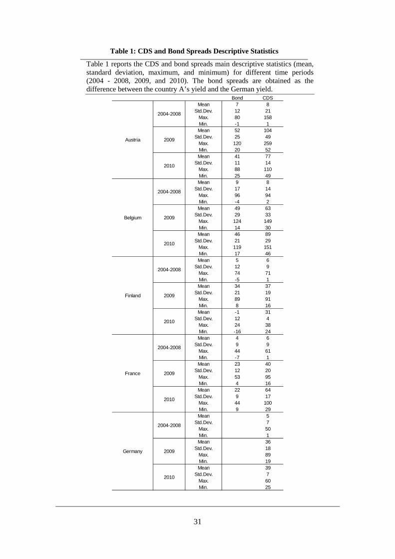
Table 1 reports the main properties of the data on bond and CDS spreads employed in

our analysis. As becomes evident from this table, average CDS rates vary substantially

across countries and periods. For the period 2004-2008, the lowest average CDS spread

was 5 basis points (bp) for Germany and the highest one was 23 bp points for Greece.

6 Mayordomo, Peña and Schwartz (2011) compare the quality of the data on CDS from different providers and find that CMA produces, on average, the most reliable data.

7

For the same period, the lowest average bond spread is 4 bp for both France and The

Netherlands,7 and the highest average is 25 bp for Greece. We note that CDS spreads

are on average higher than bond spreads in most of the countries, i.e. the basis, defined

as the difference between the CDS and bond spreads, is positive. For the second period

(Panel B), the lowest average CDS spread during that year was 36 bp for Germany and

the highest average was 190 bp for Ireland. The lowest average bond spread was 23 bp

for France and the highest was 166 bp for Greece. In this more recent period, the CDS

spreads are, again, on average, higher than the bond spreads in most of the countries.

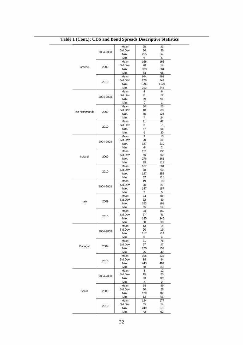
Finally, during 2010 Greece showed the maximum average credit spreads (593 bp,

being the maximum daily CDS spread at 1,126 bp) and the lowest average at 31 bp for

Finland. The maximum average CDS spread as well as the maximum daily CDS spread

corresponds to Greece (664 and 1,293 basis points, respectively). As in the other two

periods, the CDS spread is on average higher than the bond spread. These data also

show that, in general, the average credit spreads and their volatility in the peripheral

countries both increased over time.

< Insert Table 1 here>

As for the rest of the data used in the subsequent estimations, the country-stock indexes

and global risk, which is proxied by means of the implied volatility index (VIX), are

obtained from Reuters. To capture funding costs we use the difference between the 90-

day US AA-rated commercial paper interest rates for financial companies and the 90-

day US T-bill, both from Datastream. We employ liquidity measures for the sovereign

CDS and bonds which are obtained from the bond and CDS bid-ask spreads. Bond bid-

ask prices are obtained from Reuters while CDS bid-ask spreads come from CMA. To

proxy the counterparty risk on the side of CDS dealers, we employ the CDS spreads of

the 14 banks most active as dealers in the CDS market. These CDS spreads are obtained

from CMA. The information regarding the European Central Bank (ECB) bond

purchases which took place after May 2010 was obtained from the ECB webpage.

7 Recall that the bond spreads are obtained using the German bond yield as the risk free rate. This standard has been used by Balli (2008), Bernoth, von Hagen, and Schuknecht (2006), Delis and Mylonidis (2010), Favero, Pagano, and Von Thadden (2009), Foley-Fisher (2010), Geyer, Kossmeier, and Pichler (2004), among others

8

4. Are there persistent deviations between CDS and bond spreads?

Suppose that an investor buys a bond at its par value with a maturity equal to T years

and a yield to maturity equal to ytm. Also, assume that at the same time the investor

buys protection on such reference entity for T years in the CDS market and the premium

of such contract is s. The investor has eliminated the default risk associated to the

underlying bond and the investor’s net annual return is equal to ytm– s. Absent any

friction, arbitrage forces would imply that the net return should be equal to the T-year

risk-free rate, which we denote by r. Alternatively, if ytm – s < r, then by means of a

short position in the bond, writing protection in the CDS market and buying the risk-

free bond the investor could have obtained a positive profit without any risk. If, on the

contrary, ytm – s > r, the investor could obtain a certain profit by buying the risky bond,

buying protection in the CDS market and taking a short position in the risk-free bond.

Hence, in equilibrium, ytm – r = s.

In order to investigate the existence and persistency of deviations between CDS and

bond spreads, that violate the previous equilibrium relation, we apply the statistical

arbitrage test employed by Mayordomo, Peña and Romo (2011a). This test is based on a

notion of arbitrage introduced by Hogan, Jarrow, Teo and Warachka (2004) according

to which, absent market frictions, an arbitrage opportunity (in an statistical sense)

represents a zero-cost, self-financing trading opportunity that has positive expected

cumulative trading profits with a declining time-averaged variance and a probability of

loss that converges to zero as time passes. Bearing in mind that, within the logic of this

methodology, the existence of arbitrage opportunities is conditioned to the absence of

market frictions, in our application of this test, we interpret the results in a rather

agnostic way, avoiding identifying persistent deviations between both spreads with

unexploited arbitrage opportunities. Indeed, when such deviations are found, we relate

them, in a statistical sense, to several potential market frictions (see Section 5).

To test for the existence of persistent deviations from the zero-basis, we first compute

the increase in the “discounted trading profits”, which would obtain under the

assumption of no trading or funding costs, as follows. The “profits” from a given

investment strategy are defined as the basis times the contract notional value. We

compute such profits quarterly and the payment on a given date t is added to the trading

9

profits accumulated from the first investing date to the day before, t-1. The accumulated

profits constructed in this way are assumed to have been invested or borrowed at the

risk-free rate in the interim, from t-1 to t. The cumulative trading profits are then

discounted up to the initial date. The increase in the discounted cumulative trading

profits at a given date t is denoted by ∆vt and is assumed to evolve according to the

following process:

)4(tt zttv λθ σµ +=∆

for t = 0, 1, 2, …, n, with n denoting the last investment date and where zt are

innovations. We assume the following initial conditions: z0=0 and v0 = 0 (i.e. the

strategy is self-financed). Parameters θ and λ determine whether the expected trading

profits and the volatility, respectively, are decreasing or increasing over time and their

intensity. Under the assumption that zt is an i.i.d. N(0,1) variable, the expectation and

variance of the discounted incremental trading profits in equation (4) are

[ ] [ ] λθ σµ 22tvVarandtvE tt =∆=∆ , respectively.

Then, the discounted cumulative trading profits generated by a given strategy satisfy:

)5(,~0 0

22

0∑ ∑∑

= ==

∆=

n

t

n

t

n

ttn ttNvv λθ σµ

We then define the log-likelihood function for the increments in equation (5) and

estimate the parameters of interest ( )λσθµ ,,, by maximizing that function using a non-

linear optimization method based on a Quasi-Newton-type algorithm. Then, we

implement formally the notion of statistical arbitrage test outlined before through the

specification and testing of the following three simultaneous hypotheses:

[ ] .1,2

1max00)(|)(lim:3

,00)0)((lim:2

,00)]([lim:1 `

−−>⇒=<∆∆

><⇒=<

>⇒>

∞→

∞→

∞→

λθ

λθλ

µ

tvtvVarH

andortvPH

andtvEH

t

t

P

t

10

Statistical arbitrage requires that the expected cumulative discounted profits, v(t), are

positive (H1), the probability of loss converges to zero (H2), and the variance of the

incremental trading profits v(t) also converges to zero (H3).8

Hence, these three conditions must be simultaneously satisfied to have support for the

existence of persistent non-zero basis. In practice, this implies an intersection of several

sub-hypotheses. To maximize the power of the test, instead of testing whether the

previous hypotheses are simultaneously satisfied, we redefine the null hypothesis as the

absence of persistent non-zero basis and so, our test is based on the following union of

sub-hypotheses which are given by the complementary of the previous hypotheses (see

Jarrow, Teo, Tse, and Warachka, 2007):

,01:3

,02

1:3

,00:2

,0:1

2

1

≤+

≤+−

≤−≥

≤

θ

λθ

λθλ

µ

C

C

C

C

H

orH

orandH

orH

where CH1 and CH 2 are the complementary of hypotheses H1 and H2 while CH 13 and

CH 23 come from the complementary of hypothesis H3. If one of the last four hypotheses

above is satisfied, we conclude that no persistent deviations exist.

To test these hypotheses we need to estimate the p-values for the previous restrictions.

To this aim, we follow the methodology developed by Politis, Romano, and Wolf (1997

and 1999). This technique provides an asymptotically valid test under weak

assumptions.

Specifically, our analysis leads to two one-tail tests:

a) H0: no persistent deviations and HA: negative deviations (the bond spread is

significantly higher than the CDS spread);

b) H0: no persistent deviations and HA: positive deviations (the CDS spread is

significantly higher than the bond spread).

8 Implicit in hypothesis H3 is the idea that investors are only concerned about the variance of a potential decrease in wealth. Whenever the incremental trading profits are nonnegative, their variability is not penalized.

11

The results of these tests are summarized in Table 2. Panels A and B report the results

for the period ranging from January 2004 to September 2008 for negative and positive

bases, respectively. Panels C and D report the corresponding results for the period

September 2008 - September 2010. As shown in Panels A and B, we cannot reject the

null hypothesis (no persistent deviations) at any standard significance level. This result

holds irrespectively of whether we consider either positive or negative bases. However,

after the collapse of Lehman Brothers, the CDS spread is persistently higher than the

bond spread in six cases (see Panel D) while none of the countries analysed presents a

persistent negative basis, as shown in Panel C.

< Insert Table 2 here >

As a conclusion, the above results reveal that the zero-basis hypothesis cannot be

rejected when we consider the pre-crisis period although temporary non-zero basis are

not rare during that episode. This last result must be interpreted with caution since, as

argued before; a non-zero basis can not be understood mechanically as an opportunity

for arbitrage. For instance, Schonbucher (2003) and Mengle (2007) emphasize that

shorting a bond with a required maturity, even years, is not always a feasible option.

Moreover, the fact that non-zero basis seem to appear during the crisis period may be

symptomatic of the presence of other restrictions and frictions that prevent a perfect

timeless alignment between the CDS and the bond spreads and whose relevance may

have been exacerbated by the crisis itself. This could be the case, for instance, of

funding costs, differences in liquidity across markets and counter-party risk in the CDS

market. In the following section we test for the significance of these (and other) factors,

as potential explanatory variables for the cases of non-zero basis detected during the

crisis.

5. The determinants of the basis

In this section we test whether the differences between the CDS and bond spreads are

purely random or, alternatively, whether they are related to any market-specific or

global factors. Specifically, we consider the following potential explanatory factors:

12

a. Counterparty Risk. In principle, the higher the counterparty risk of the seller of

protection via CDS is, the lower should be the CDS spread charged as a result of the

lower quality of the protection. We test for this effect by using the first principal

component obtained from the CDS spreads of the main 14 banks which act as dealers in

that market.9 The first principal component series should reflect the common default

probability and, hence, it is akin to an aggregate measure of counterparty risk.10

Actually, the first PC for the series of CDS spreads of this set of dealers explains 87.5%

of the total variance of the observed variables.

b. Liquidity. In theory, one would expect that higher liquidity in the bond market

relative to the CDS market would go hand in hand with a higher basis, since a more

liquid bond implies a higher price and, hence, a lower bond spread. To test for this

relative liquidity effects, we construct a ratio of relative liquidity between the bond and

the CDS. Specifically, the degree of liquidity in the CDS market is proxied by the

relative bid-ask spread which is obtained as the ratio between the bid-ask spread of the

CDS premium and the mid-premium, i.e. (Ask-Bid)/((Ask+Bid)/2). The higher this ratio

is, the lower is the degree of liquidity in the CDS market. A similar measure of liquidity

is computed for the bond market and the ratio between both is taken as indicative of the

relative liquidity in the bond market vis-à-vis the CDS market. As this ratio rises,

liquidity in the bond market relative to the CDS market falls and so does the basis.

c. Financing Costs: One would expect that higher financing costs would lower the

demand for bonds, as buying them require funding, and could lead to a decrease in

prices, and hence, to higher bond spreads. The effect of funding costs on CDS spreads

should be lower given that in this case the required amount of funding to get the same

(gross) risk position is lower (i.e. risk-leverage is higher in the case of the CDS

investment). For this reason, an increase in financing costs would have a negative effect

on the basis. Due to the difficulty in obtaining data on institution-level funding

constraints, we use the spread between financial commercial paper and T-bill rates as a

9 The 14 main dealers are: Bank of America, Barclays, BNP Paribas, Citigroup, Credit Suisse, Deutsche Bank, Goldman Sachs, HSBC, JP Morgan, Morgan Stanley, Royal Bank of Scotland, Societé Generale, UBS, and Wachovia/Wells Fargo. These dealers are the most active global derivatives dealers and are known as the G14 (see for instance ISDA Research Notes (2010) on the Concentration of OTC Derivatives among Major Dealers). 10 The use of the dealers’ CDS spreads as a proxy of counterparty risk is based on the Arora, Ghandi, and Longstaff (2009) study which analyses the existence of counterparty risk in the corporate CDS market.

13

common proxy for the funding constraints faced by financial intermediaries, as in

Acharya, Schaefer and Zhang (2006). Specifically, we use the spread between the 90-

day US AA-rated commercial paper interest rates for the financial companies and the

90-day US T-bill.

d. Domestic and global risk premiums: As additional potential explanatory variables

for the basis, we consider a measure of the country and global risk premium. If both the

CDS and bond spreads are prices for the same credit risk, the effect of the country-

specific and global risk premiums on the basis should be non-significantly different

from zero. However, in order to control for the fact that this idiosyncratic and global

volatility could be priced differently in the two markets, we use the previous risk factors

as additional explanatory variables. The country-specific risk premium is proxied by

means of the stock market volatility. The global risk premium or global risk is proxied

by means of the VIX Index. The correlation between the VIX Index and the

counterparty risk variable is around 0.8. Thus, in order to avoid any multicollinearity

problem, we modify the counterparty-risk variable and define it as the residual of the

regression of the first principal component CDS spreads corresponding to the main CDS

dealers onto the VIX Index such that counterparty risk and VIX are now orthogonal

variables and the counterparty risk is not related to changes in the perception of global

risk.

e. Bond-CDS Spillovers: We here use the notion of spillovers between the CDS and

the bond markets as the variation in the CDS (bond) spread that is not attributable to its

past values but to contemporary shocks to the bond (CDS) spread. To measure such

spillovers or contagion-effects, we use a procedure based on Diebold and Yilmaz’s

(2010) methodology and described in Appendix A.1. The Bond-CDS spillovers variable

is obtained after dividing the spillovers from the changes in bond spread to the changes

in CDS spread relative to spillovers from the CDS to the bond spread changes. This

variable reflects the increase in a given spread due to a direct effect of the other market.

We work in relative terms because the dependent variable is the difference between

both credit spreads. A positive (negative) sign implies that when the ratio increases, that

is, the shock transmission from the bond market to the CDS market is stronger (weaker)

than in the opposite direction, then the basis widens (narrows) , or in other words, the

CDS spread increases (decreases) with respect to the bond spread.

14

f. Lagged basis: The lag of the basis should absorb any lagged information transmitted

into the current observation. It also permits us to test the speed of adjustment of a

positive and negative basis. Due to the existence of persistent deviations between CDS

and bond spreads documented in Section 4, we expect a positive sign.

We estimate the coefficients for the above variables of interest using a fixed-effects

estimation procedure that is robust to heteroskedasticity. We use the bootstrap

methodology to correct for any potential bias in the standard errors due to the use of

generated regressors. We report the results for different time periods in Table 3.

Columns 1, 2, and 3 refer to the period which spans from Jan-2004 to Sep-2010, Jan-

2007 to Sep-2010, and Jan-2008 to Sep-2010, respectively.

Interestingly, we observe that the relevance of the counterparty risk indicator increases

in the last part of the sample. In particular, when we restrict the sampling period to

January 2008 – September 2010, the counterparty risk proxy has a negative, as

expected, and significant effect. Although non-significant at 5% level, the relative

liquidity has a negative effect, as expected. Funding costs have a negative effect, as

expected, in the three sub-samples, although non-significant. The global risk variable is

not significant in any of the three scenarios which may suggest that both markets reflect

global risk to a similar extent. Similarly, the country risk premium, proxied by the

squared of the stock index returns, seems not to be priced differently in both markets.

We also find that the shock-spillovers ratio has a positive and significant effect. That is,

when the shock transmission from the bond to the CDS market dominates the shock

transmission in the opposite direction, then the basis widens. One economic implication

of this empirical finding is that in periods in which the ratio of spillovers from the bond

market to the CDS market increases we observe ceteris paribus a CDS’s market relative

overreaction and thus, the CDS spread will signal a stronger default probability for a

given reference name than the bond spread. In line with the results of the previous

section, we find a high level of persistency in the basis. That is, there is a relatively low

speed of adjustment towards the long-run bond-CDS equivalence relation. Finally, the

constant term reflects whether the basis differs, on average, from zero and the

magnitude of such deviation. The results show that for the first two sub-periods the

basis does not significantly differs from zero, that is, the bond-CDS equivalence relation

holds when we take into account the market frictions described above and the costs that

15

are needed to trade the basis. Although in the third time-period the basis is on average

significantly positive, its magnitude is low relative to the average basis during that

period (1.4 basis points relative to 7.7 basis points). The relatively high R-square of this

regression is mainly due to the effect of the lagged basis and the fixed effects. However,

it should be noted that the explanatory variables retain a relatively high explanatory

power even when we ignore the lagged basis and the fixed effects, in which case the R-

square is around 0.3. Actually, this is of a similar magnitude of the one reported by

Trapp (2009) on a daily basis for corporates using firm fixed-effects but ignoring the

effect of the lagged basis.

< Insert Table 3 here >

We next study whether there is any asymmetry between positive and negative bases.

For this purpose, we repeat the previous regression but we now distinguish between

positive and negative lagged bases. In particular, we allow for two separate variables:

Positive basis = max(Basis,0) and Negative basis= min(Basis,0). The results

corresponding to the new estimation are reported in Table 4. The difference between

the coefficient referred to a positive basis and the one referred to a negative basis is

significantly higher than zero for the three time periods considered in Table 4. As the

theory suggests, apparently, it is more difficult to close a positive basis than the

opposite. The reason is that to close the former deviation an investor would need to take

short positions in CDS (sell protection) and bonds, respectively. Similar results are

obtained for the three sampling periods considered (January 2004 – September 2010 in

Column (1); January 2007 – September 2010 in Column (2); and January 2008 –

September 2010 in Column (3)).

< Insert Table 4 here >

6. Price-discovery analysis

An efficient price discovery process is characterized by a quick adjustment of market

prices from the old to the new equilibrium as new information arrives (see e.g. Yan and

Zivot, 2007). The previous literature that has tried to measure this form of market-

efficiency has focused on static price-discovery analyses. In contrast, we here show that

16

the price discovery process in the markets for sovereign credit risk in the EU does not

show a time-invariant pattern (Section 6.1). Given this finding, we then try to identify

the effect of several potential explanatory variables of the price-discovery metrics

obtained in the previous step (Section 6.2).

6.1. A dynamic price-discovery metric

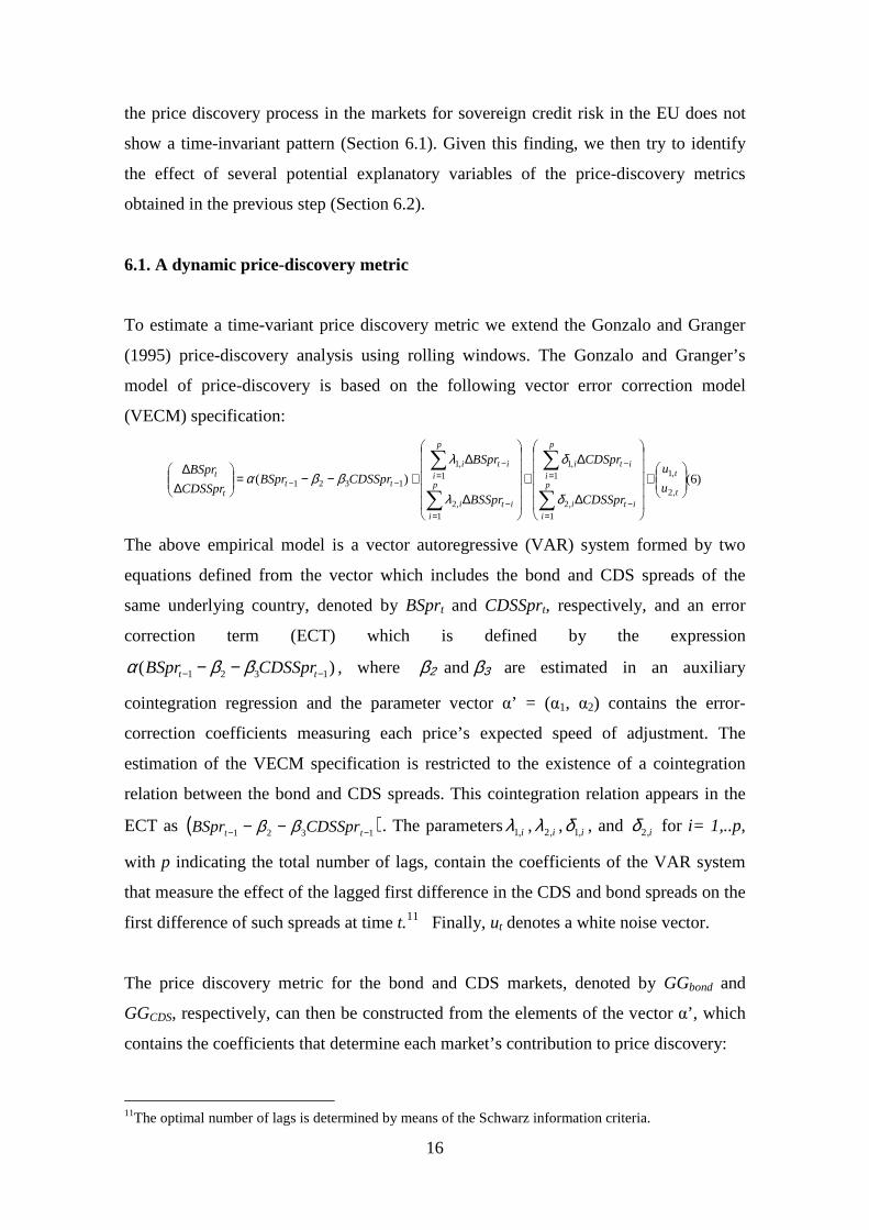
To estimate a time-variant price discovery metric we extend the Gonzalo and Granger

(1995) price-discovery analysis using rolling windows. The Gonzalo and Granger’s

model of price-discovery is based on the following vector error correction model

(VECM) specification:

)6()(,2

,1

1,2

1,1

1,2

1,1

1321

+

∆

∆+

∆

∆+−−=

∆∆

−=

−=

−=

−=

−−

∑

∑

∑

∑t

t

it

p

ii

it

p

ii

it

p

ii

it

p

ii

ttt

t

u

u

CDSSpr

CDSpr

BSSpr

BSpr

CDSSprBSprCDSSpr

BSpr

δ

δ

λ

λββα

The above empirical model is a vector autoregressive (VAR) system formed by two

equations defined from the vector which includes the bond and CDS spreads of the

same underlying country, denoted by BSprt and CDSSprt, respectively, and an error

correction term (ECT) which is defined by the expression

)( 1321 −− −− tt CDSSprBSpr ββα , where β2 and β3 are estimated in an auxiliary

cointegration regression and the parameter vector α’ = (α1, α2) contains the error-

correction coefficients measuring each price’s expected speed of adjustment. The

estimation of the VECM specification is restricted to the existence of a cointegration

relation between the bond and CDS spreads. This cointegration relation appears in the

ECT as ( )1321 −− −− tt CDSSprBSpr ββ . The parameters i,1λ , i,2λ , i,1δ , and i,2δ for i= 1,..p,

with p indicating the total number of lags, contain the coefficients of the VAR system

that measure the effect of the lagged first difference in the CDS and bond spreads on the

first difference of such spreads at time t.11 Finally, ut denotes a white noise vector.

The price discovery metric for the bond and CDS markets, denoted by GGbond and

GGCDS, respectively, can then be constructed from the elements of the vector α’, which

contains the coefficients that determine each market’s contribution to price discovery:

11The optimal number of lags is determined by means of the Schwarz information criteria.

17

21

1

21

2 ;αα

ααα

α+−

−=+−

= CDSBond GGGG

Given that GGBond + GGCDS = 1, we would conclude that the bond (CDS) market leads

the price discovery process whenever GGBond is higher (lower) than 0.5. The intuition

for this is the following. The larger the speed in eliminating the price difference from

the long-term equilibrium attributable to a given market, the higher the corresponding α

according to (6), and the higher is the price discovery metric.

In order to apply the methodology outline above to provide a dynamic metric of price-

discovery leadership in the two markets at stake, we estimate the system in equation (6)

using rolling windows with different lengths: 500, 750, and 1,000 days. To do so, we

first need to check for the order of integration of the CDS and bond spreads and then for

the existence of a cointegration relation. Using rolling windows with a length of 500

observations (henceforth, we use this as our baseline window-length), we find that the

bond spread is integrated of order one (non-stationary) in all the countries and dates,

except for Greece in 42 dates, or equivalently, in 3.5% of the windows the bond spread

of Greece is stationary at a 5% confidence level. Regarding the CDS spread, it is

integrated of order one in all the dynamic sub-samples considered and for all the

countries at a significance level of 5%.12

We next apply the cointegration test to a total of 1,203 500-day windows for each of the

ten countries and find cointegration between both spreads in 7,284 cases (61% of the

total). In particular, the country with the lowest (highest) percentage of cointegration

relations is France (The Netherlands) with cointegration in 38% (82%) of the windows.

As we increase the window length, we find a higher number of cointegration relations.

For instance, for a window length of 750 (1,000) cointegration exists in 67% (76%) of

the cases.

Figure 1 shows the average price discovery metrics obtained for the three different

window-lengths. In particular, we report a 30-day moving average of the mean price-

discovery metrics which is obtained as an equally weighted mean across the ten euro

12 The number of lags employed in the Granger causality test is chosen according to the Schwarz information criterion.

18

area countries. A first interesting feature is that the estimated metrics do not seem to be

very sensitive to the window length. Based on this, in the remaining of the paper we

focus on 500-day windows.

An important message steaming from Figure 1 is that the price discovery metrics are not

static but rather evolve over time, with the relative leadership of the CDS market in the

process of price-discovery being more pronounced around some specific dates.

Specifically, before the summer of 2007 the CDS market clearly leads sovereign risk

price discovery. This finding is consistent with the results reported by, e.g., Blanco,

Brennan and Marsh (2005), Zhu (2006), or Norden and Weber (2009) in the context of

the corporate debt markets. The first noticeable rise in the relative leadership of the

bond market took place around February 2008, around the collapse of Bear Stearns.

Afterwards, in September 2008, coinciding with the fall of Lehman Brothers and AIG

the bond price discovery metric again jumps to reach its highest value at the end of

2008. This pattern suggests that during these two specific episodes, Bear Stearns and

Lehman-AIG, the bond spread led, although by a small margin, the price discovery

process. Next, we observe another rebound in the price-discovery indicator in Figure 1

around April 2010, coinciding with the worst moments of the Greek sovereign debt

crisis. However, right after the approval of a rescue package for Greece by the European

Union and the International Monetary Fund, the CDS market started to regain its

leadership role.13

< Insert Figure 1 here >

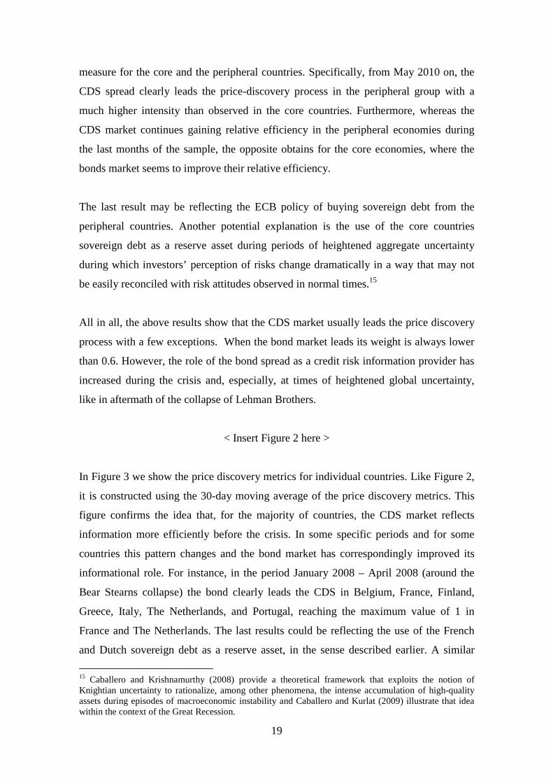
Figure 2 shows the estimated price-discovery metric for two groups of countries in the

sample, peripheral and central countries.14 Except for some gaps between the two

country-groups price-discovery metrics witnessed before the crisis (around 2006 and the

first half of 2007) the pattern followed by the metrics corresponding to the two groups

of countries has been remarkably similar for most part of the period under study.

However, in the final part of the sample period (from around the spring of 2010

onwards) the empirical model detects some decoupling between the price-discovery

13 In line with Mayordomo, Peña, and Romo (2011b) these results confirm the role of the bond markets during this period as a fair measure of credit risk. 14 The peripheral group includes Ireland, Italy, Greece, Portugal and Spain. The core group includes Austria, Belgium, Finland, France and The Netherlands. The window length in all cases is 500 days.

19

measure for the core and the peripheral countries. Specifically, from May 2010 on, the

CDS spread clearly leads the price-discovery process in the peripheral group with a

much higher intensity than observed in the core countries. Furthermore, whereas the

CDS market continues gaining relative efficiency in the peripheral economies during

the last months of the sample, the opposite obtains for the core economies, where the

bonds market seems to improve their relative efficiency.

The last result may be reflecting the ECB policy of buying sovereign debt from the

peripheral countries. Another potential explanation is the use of the core countries

sovereign debt as a reserve asset during periods of heightened aggregate uncertainty

during which investors’ perception of risks change dramatically in a way that may not

be easily reconciled with risk attitudes observed in normal times.15

All in all, the above results show that the CDS market usually leads the price discovery

process with a few exceptions. When the bond market leads its weight is always lower

than 0.6. However, the role of the bond spread as a credit risk information provider has

increased during the crisis and, especially, at times of heightened global uncertainty,

like in aftermath of the collapse of Lehman Brothers.

< Insert Figure 2 here >

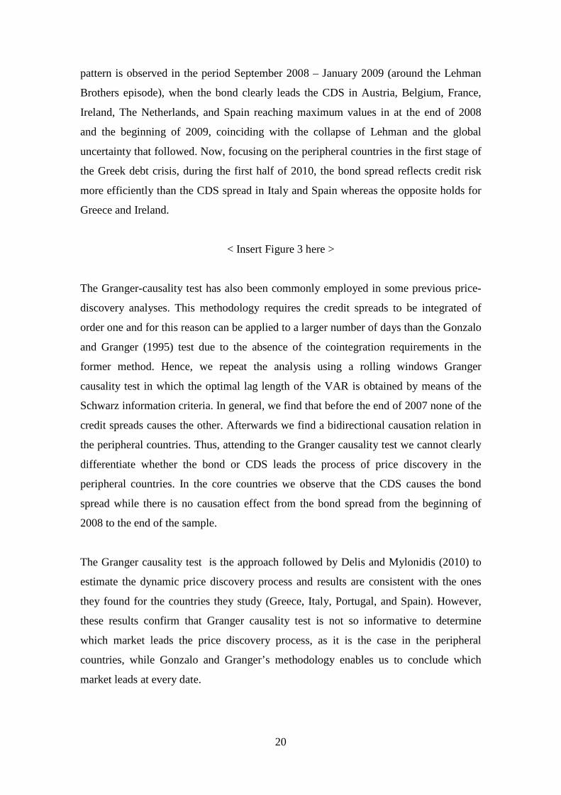
In Figure 3 we show the price discovery metrics for individual countries. Like Figure 2,

it is constructed using the 30-day moving average of the price discovery metrics. This

figure confirms the idea that, for the majority of countries, the CDS market reflects

information more efficiently before the crisis. In some specific periods and for some

countries this pattern changes and the bond market has correspondingly improved its

informational role. For instance, in the period January 2008 – April 2008 (around the

Bear Stearns collapse) the bond clearly leads the CDS in Belgium, France, Finland,

Greece, Italy, The Netherlands, and Portugal, reaching the maximum value of 1 in

France and The Netherlands. The last results could be reflecting the use of the French

and Dutch sovereign debt as a reserve asset, in the sense described earlier. A similar

15 Caballero and Krishnamurthy (2008) provide a theoretical framework that exploits the notion of Knightian uncertainty to rationalize, among other phenomena, the intense accumulation of high-quality assets during episodes of macroeconomic instability and Caballero and Kurlat (2009) illustrate that idea within the context of the Great Recession.

20

pattern is observed in the period September 2008 – January 2009 (around the Lehman

Brothers episode), when the bond clearly leads the CDS in Austria, Belgium, France,

Ireland, The Netherlands, and Spain reaching maximum values in at the end of 2008

and the beginning of 2009, coinciding with the collapse of Lehman and the global

uncertainty that followed. Now, focusing on the peripheral countries in the first stage of

the Greek debt crisis, during the first half of 2010, the bond spread reflects credit risk

more efficiently than the CDS spread in Italy and Spain whereas the opposite holds for

Greece and Ireland.

< Insert Figure 3 here >

The Granger-causality test has also been commonly employed in some previous price-

discovery analyses. This methodology requires the credit spreads to be integrated of

order one and for this reason can be applied to a larger number of days than the Gonzalo

and Granger (1995) test due to the absence of the cointegration requirements in the

former method. Hence, we repeat the analysis using a rolling windows Granger

causality test in which the optimal lag length of the VAR is obtained by means of the

Schwarz information criteria. In general, we find that before the end of 2007 none of the

credit spreads causes the other. Afterwards we find a bidirectional causation relation in

the peripheral countries. Thus, attending to the Granger causality test we cannot clearly

differentiate whether the bond or CDS leads the process of price discovery in the

peripheral countries. In the core countries we observe that the CDS causes the bond

spread while there is no causation effect from the bond spread from the beginning of

2008 to the end of the sample.

The Granger causality test is the approach followed by Delis and Mylonidis (2010) to

estimate the dynamic price discovery process and results are consistent with the ones

they found for the countries they study (Greece, Italy, Portugal, and Spain). However,

these results confirm that Granger causality test is not so informative to determine

which market leads the price discovery process, as it is the case in the peripheral

countries, while Gonzalo and Granger’s methodology enables us to conclude which

market leads at every date.

21

6.2. An analysis of the determinants of the market leadership in price-discovery

In this section we aim at providing a (partial) explanation of the dynamic pattern of the

price-discovery metrics estimated before, by regressing them on some potential

explanatory factors.

Specifically, for each country, we construct a dummy variable that takes a value of 1

when the bond market reflects information more efficiently than the CDS market and 0

otherwise. This dummy is constructed on the basis of a rolling window estimation using

1,000 observations,16 and then it is used as the dependent variable in a Logit regression

that includes as regressors the same used in the regression contained in Table 2 with the

exception of the lagged basis and the relative spillovers measure. The last measure is

not included due to potential endogeneity problems. We consider these regressors

because they have been found to have a significant effect on the deviations from a zero-

basis. Hence, as this reflects that the effect of such regressors is not reflected in the

same way in the two markets, it seems natural to consider that one market could capture

better than the other the effect of each determinant of the basis. Additionally, as

mentioned informally before, the role of the two markets providing efficient

information on credit risk could have been affected by the interventions of the ECB

after May 2010 buying sovereign debt. For this reason we also use as an explanatory

variable the amount of sovereign debt purchased by the ECB. Additionally, we

distinguish the effect of such potential determinants of the price discovery metrics on

peripheral and core countries.

The results are reported in Table 5. Column 1 contains the results for the period

December 2007 – September 2010.17. Column 2 shows the results for the period

spanning from September 2008 – September 2010. Columns 3 and 4 show the results

16 When faced with missing values (due to a lack of cointegration relation between the CDS and the bond spreads), the value of the dummy is imputed according to the Granger-causality analysis performed earlier. For the remaining missing values, the value of the dummy is imputed whenever there is another observed value within the next month which coincides with the previous price discovery value observed and persists at least in the next ten observations. If after a given date there are not cointegration relations up to the end of the sample we do not impute any value. For sake of the robustness of this procedure, we use the 1,000-observation estimation. We do not employ the price discovery metric directly, which is a concrete value comprised between 0 and 1, but instead assign a value one or zero to such metrics, thus softening such strong assumption. We impute a total of 885 observations (i.e. 14% of the observations), out of which 197 of the observations are imputed by means of the Granger-causality test and 688 by the alternative method. 17 Notice that in choosing the length of the first period we are restricted by the (conservative) choice of a 1000-day window.

22

obtained for the subgroups of core and peripheral countries, respectively, for the period

December 2007 – September 2010.

One might expect that the higher the counterparty risk the lower should be the ability of

the CDS market to reflect adequately the credit risk. The sign is the expected (positive)

and significant in Columns (1) and (2) referred to the whole group of countries. In line

with the results obtained in Table 3, as we use a period closer to the collapse of Lehman

Brothers and the European sovereign debt crisis the coefficient increases and becomes

more significant. We also observe remarkable differences across the core (Column 3)

and peripheral (Column 4) countries. The effect of counterparty risk is positive for both

groups of countries but is only significant for the group of peripheral countries. Thus,

counterparty risk significantly lowers the ability of the CDS spreads to reflect

adequately credit risk in the peripheral countries but not in the core countries.

We find that a low degree of liquidity in the bond market relative to the CDS market

affects negatively to the price discovery metric. The effect is higher in Column (2) than

in Column (1), possibly due to the higher influence of low liquidity in CDS markets

around the Lehman Brothers collapse and the rescue of Greece. Surprisingly, for the

group of core countries (Column 3) the effect of the liquidity ratio is positive, being

negative and significant for the group of peripheral countries (Column 4), as the theory

would suggest.

Funding costs affect negatively to the bond buyers contrary to the CDS market which

allows for higher-leveraged positions. For this reason the funding costs affect negatively

to the ability of the bonds market for anticipating the credit risk relative to the CDS

market. The effect of this variable dilutes as the sample period comprises the European

sovereign debt crisis. The magnitude of the coefficient for the funding cost variable is

similar for the two groups of countries. This result suggests that funding costs affect

similarly to the capacity of price discovery of credit spread for the different countries.

In line with the results obtained by Mayordomo, Peña and Romo (2011b) the bond

spreads tend to reflect credit risk more efficiently than CDS spreads during periods of

high global risk (high values of the VIX Index). This result is consistent for the four

regression specifications. The country specific risk premium proxied by means of the

23

squared returns of the national stock index is not significant at 5% significance level but

the related coefficient has different signs for the core (positive sign) and peripheral

(negative sign) countries.

If the ECB is buying debt independently of the price, information derived from such

market could become less revealing of the fundamental value of the traded security.

This hypothesis is confirmed by the significant and negative sign of the variable

representing the amount of sovereign debt purchased by the ECB which is obtained in

the four columns. Interestingly, the magnitude for such coefficient differs between the

core and peripheral countries being the latter magnitude significantly higher than the

former. This result may be reflecting the ECB policy of buying sovereign debt from the

peripheral countries

< Insert Table 5 here >

7. Conclusions

This paper analyzes the extent to which the sovereign Credit Default Swap (CDS) and

bond markets reflect the same information on their prices in the context of the European

Monetary Union. The main results can be summarized as follows.

We first test the “no-arbitrage” theoretical relation that should exist between the bond

and the CDS spreads in a frictionless environment since both spreads are supposed to be

the prices for the same credit risk. Our results show that after the subprime crisis there

are persistent deviations from that theoretical parity relation that were absent before. In

particular, we find evidence in favour of a persistent positive basis for the crisis period

in a number of countries.

Based on the previous finding, we analyse the role of some potential determinants of the

basis, including several different types of risks (counterparty, country-idiosyncratic and

global) and market frictions. In particular, we find that the counterparty risk indicator

has a negative and significant effect on the basis, especially during the most recent

period. Both funding costs and a low liquidity in the bond market relative to the CDS

market also have a negative effect on the basis. In periods in which shocks originated in

24

the bond market are transmitted into the CDS market, which we interpret as spillovers

or contagion-effects, we find an overreaction-effect in this last market. Finally, we show

that the speed of reversion of the basis is asymmetric, with positive bases typically

requiring a longer time to diminish.

Finally, we conduct a dynamic analysis of market leadership in the price discovery

process. An important result here is that the price discovery process is state-dependent.

Specifically, the levels of counterparty and global risk, funding costs, market liquidity

and the volume of debt purchases by the European Central Bank in the secondary

market following the rescue of the Greek economy in May 2010 are all found to be

significant factors in determining which market leads price discovery.

25

References

1. Ammer, J. and Cai, F. (2007) “Sovereign CDS and Bond Pricing Dynamics in

Emerging Markets: Does the Cheapest-to-Deliver Option Matter?”, Board of

Governors of the Federal Reserve System. International Finance Discussion Papers

Number 912.

2. Arora, N., Gandhi, P., and Longstaff, F. (2009), "Counterparty Credit Risk and the

Credit Default Swap Market". Working Paper, UCLA.

3. Bai, J., and Collin-Dufresne (2009) “The Determinants of the CDS-Bond Basis

during the Financial Crisis of 2007-2009”. Working Paper.

4. Balli, F. (2008) “Spill over Effects of Government Bond Yields in Euro Zone. Does

Full Financial Integration Exist in European Government Bond Markets?” Working

Paper.

5. Bernoth, K., von Hagen J. and Schuknecht, L. (2006) “Sovereign Risk Premiums in

the European Government Bond Market”. GESY Discussion paper 151.

6. Beber, A., Brandt, M.W. and Kavajecz, K.A. (2009) “Flight-to-quality or flight-to-

liquidity? Evidence from the Euro-area bond market”. Review of Financial Studies,

(forthcoming) doi:10.1093/rfs/hhm088.

7. Belke, A., and Gokus, C. (2011) “Volatility Patterns of CDS, Bond, and Stock

Markets Before and During the Financial Crisis: Evidence from Major Financial

Institutions”. DIW Berlin. Discussion Papers.

8. Blanco, R., Brennan, S., Marsh, I. W., (2005) “An Empirical Analysis of the

Dynamic Relationship between Investment Grade Bonds and Credit Default

Swaps”. Journal of Finance 60, 2255-2281.

9. Bowe, M., Klimaviciene, A., and Taylor, A. P. (2009) “Information Transmission

and Price Discovery in Emerging Sovereign Credit Risk Markets”. Working Paper.

10. Caballero, R., and A. Krishnamurthy (2008) “Collective Risk Management in a

Flight to Quality Episode”. Journal of Finance 83, 2195-2230.

11. Caballero, R., and P. Kurlat (2009) “The ‘Surprising’ Origin and Nature of

Financial Crises: A Macroeconomic Policy Proposal”, in Financial Stability and

Macroeconomic Policy, Federal Reserve Bank of Kansas City.

12. Caceres, C., Guzzo, V., and Segoviano, M. (2010) “Sovereign Spreads: Global Risk

Aversion, Contagion, or Fundamentals”. IMF Working Paper.

13. Chan-Lau, J.A. and Kim, Y.S. (2004) “Equity Prices, Credit Default Swaps, and

Bond Spreads in Emerging Markets”. IMF, Working Paper.

26

14. Chen, L., Lesmond, D.A. and Wei, J. (2007) “Corporate Yield Spreads and Bond

Liquidity”. Journal of Finance, 62, 119-149.

15. Collin-Dufresne, P., Goldstein, R., and Martin, J.S. (2001) “The Determinants of

Credit Spread Changes”. Journal of Finance, 56, 1926-1957.

16. Codogno, L., Favero, C. and Missale, A. (2003) “Government bond spreads”.

Economic Policy, 18, 504-532.

17. Delatte, A. L., Gex, M., and Lopez-Villavicencio, A. (2010) “Has the CDS Market

Amplified the European Sovereign Crisis?” A Non-Linear Approach”. Working

Paper.

18. Delis, M. D., and Mylonidis, N. (2010) “The Chicken or the Egg? A Note on the

Dynamic Interrelation between Government Bond Spreads and Credit Default

Swaps”. Finance Research Letters, forthcoming.

19. Diebold, F. X., Yilmaz, K., (2010) “Better to Give than to Receive: Predictive

Directional Measurement of Volatility Spillovers”. Tüsiad-Koç University

Economic Research Forum Working Paper Series.

20. Diebold, F. X., Yilmaz, K., (2009) “Measuring Financial Asset Return and

Volatility Spillovers, with Application to Global Equity Markets”. The Economic

Journal, 119, 158–171.

21. Elton, E. J., Gruber, M. J., and Agrawal, D. (2001) “Explaining the Rate Spread on

Corporate Bonds”. Journal of Finance 56, 247-278.

22. Ericsson, J., Jacobs, K. and Oviedo-Helfenberger (2009) “The Determinants of

Credit Default Swap Premia”, Journal of Financial and Quantitative Analysis, 44,

109-132.

23. European Central Bank (2009) Credit Default Swaps and Counterparty Risk, August

2009.

24. Favero, C., Pagano, M. and Von Thadden E.-L. (2009) “How Does Liquidity Affect

Government Bond Yields?” Journal of Financial and Quantitative Analysis

(forthcoming)

25. Foley-Fisher, N. (2010) “Explaining Sovereign Bond-CDS Arbitrage Violations

During the Financial Crisis 2008-09”. Working Paper.

26. Fontana, A., and Scheicher, M. (2010) “An Analysis of Euro Area Sovereign CDS

and their Relation with Government Bonds”. European Central Bank, Working

Paper.

27

27. Forte, S. and Peña, J.I. (2009) “Credit Spreads: Theory and Evidence about the

Information Content of Stocks, Bonds and CDSs”, Journal of Banking and Finance,

33, 2013-2025.

28. Geyer, A. Kossmeier, S. and Pichler, S. (2004) “Measuring Systematic Risk in

EMU Government Yield Spreads”. Review of Finance, 8, 171–197.

29. Hasbrouck, J. (1995) “One security, many markets: Determining the contributions to

price discovery”, Journal of Finance, 50, 1175-1199.

30. Hogan, S., Jarrow, R., Teo, M, and Warachka, M. (2004), “Testing Market

Efficiency using Statistical Arbitrage with Applications to Momentum and Value

Trading Strategies”, Journal of Financial Economics, 73, 525-565.

31. ISDA Research Notes (2010). Concentration of OTC Derivatives among Major

Dealers.

32. Jarrow, R. A., Teo, M., Tse, Y. K., and Warachka, M. (2007) “Statistical Arbitrage

and Market Efficiency: Enhanced Theory, Robust Tests and Further Applications”.

Working Papers Series, Singapore Management University.

33. Küçük, U. N. (2010). “Non-Default Component of Sovereign Emerging Market

Yield Spreads and its Determinants: Evidence from Credit Default Swap Market”.

Journal of Fixed Income 19, 44-66.

34. Levy, A. (2009) “The CDS Bond Basis Spread in Emerging Markets: Liquidity and

Counterparty Risk”. Working Paper.

35. Longstaff, F. A. (2010) “The Subprime Credit Crisis and Contagion in Financial

Markets”. Journal of Financial Economic 97, 436-450.

36. Longstaff, F.A., Mithal, S. and Neis, E. (2005), "Corporate Yield Spreads: Default

Risk or Liquidity? New Evidence from the Credit Default Swap Market", Journal of

Finance 60, 2213-2253.

37. Longstaff, F. A., Pan, J., Pedersen, L. H., and Singleton, K. J., (2010) “How

Sovereign is Sovereign Credit Risk”, Working Paper, UCLA Anderson School, MIT

Sloan School, NYU Stern School, and Stanford Graduate School of Business.

38. Mayordomo, S., Peña, J. I. and Romo, J., (2011a) “A New Test of Statistical

Arbitrage with Applications to Credit Derivatives Markets”. Working Paper.

Available at SSRN: http://ssrn.com/abstract=1796791.

39. Mayordomo S., Peña, J. I., and Romo J. (2011b), “The Effect of Liquidity on the

Price Discovery Process in Credit Derivatives Markets in Times of Financial

Distress”. European Journal of Finance, forthcoming.

28

40. Mayordomo, S., Peña, J. I., and Schwartz, E. S. (2011), “Towards a Common

European Monetary Union Risk Free Rate”. Working Paper UCLA, Universidad

Carlos III de Madrid.

41. Mengle, D., 2007. Credit derivatives: an overview. Economic Review, Federal

Reserve Bank of Atlanta, issue Q4, 1 - 24.

42. Nashikkar, A., Subrahmanyam, M., and Mahanti, S. (2008) “Limited Arbitrage and

Liquidity in the Market for Credit Risk”. Working Paper, New York University.

43. Norden, L. and Weber, M. (2004) “Informational Efficiency of Credit Default Swap

and Stock Markets: The Impact of Credit Ratings Announcements”, Journal of

Banking and Finance, 28, 2813-2843.

44. Politis, D. N., Romano, J. P., (1994). The stationary bootstrap. Journal of the

American Statistical Association 89, 1303-1313.

45. Politis, D. N., Romano, J. P., Wolf, M., (1997). Subsampling for heteroskedastic

time series. Journal of Econometrics 81, 281-317.

46. Politis, D. N., Romano, J. P., Wolf, M., (1999). Subsampling intervals in

autoregressive models with linear time trend. Econometrica 69, 1283-1314.

47. Schonbucher, P. J., 2003. Credit derivatives pricing models: Models, pricing,

implementation. Wiley Finance, New York.

48. Trapp, M. (2009) “Trading the bond-CDS Basis – The Role of Credit Risk and

Liquidity”. Centre for Financial Research – Working Paper No. 09-16.

49. Yan, B. and Zivot, E. (2007) “The Dynamics of Price Discovery”, University of

Washington Working Paper Series.

50. Zhu, H., (2006) “An Empirical Comparison of Credit Spreads between the Bond

Market and the Credit Default Swap Market”. Journal of Financial Services

Research 29, 211-235.

29

Appendix A.1

Estimation of the spillovers between the CDS and bonds markets

We use a notion of spillover effects according to which such effects are defined from a

variance decomposition associated with an N-variable vector auto regression following

the methodology employed by Diebold and Yilmaz (2009) and later improved in

Diebold and Yilmaz (2010) by measuring directional spillovers in a generalized VAR

framework that eliminates the possible dependencies of results on ordering. The

spillovers between the CDS and bond spreads here estimated can be interpreted as the

degree of variation in the changes of the CDS (bond) spreads that is not attributable to

their historical information but to contemporary shocks (innovations) in the changes of

the bond (CDS) spreads. This indicator of contagion takes higher values as the intensity

of the contagion effect which is caused by the specific shocks of the bond (CDS) market

increases. In the extreme case in which there is no contagion from the bond to the CDS

market the indicator series is equal to zero.

In particular, we first consider a covariance stationary N-variable VAR (p):

)1(1∑

=− +Φ=

p

ititit XX ε

where tX denotes a vector of stationary changes in the CDS and bond spreads of a

given country and ),0(~ Σε is a vector of independently and identically distributed

disturbances such that the moving average representation is ∑∞

=−=

01,

itit AX ε where the

NxN coefficient matrices Ai obey the recursion ,...2211 pipiii AAAA −−− Φ++Φ+Φ= with

A0 being an NxN identity matrix and Ai=0 for i<0. Thus, the error from the forecast of

tX at the H-step-ahead horizon, conditional on information available at t-1, can be

expressed as ∑=

−+=H

hhHthHt A

0, ,εξ and the variance covariance matrix of the total

forecasting error is computed as ∑=

Σ=H

hhhHt AACov

0, ,')(ξ where Σ is the variance-

covariance matrix of the error term in equation (1), tε .

The moving average coefficients are the key to understanding the dynamics of the

system. We rely on variance decompositions, which allow us to parse the forecast error

30

variances of each variable into parts attributable to the various system shocks. By means

of this variance decomposition we can obtain the proportion of the H-step-ahead error

variance in forecasting Xi that is due to shocks to Xj, ,ij ≠∀ for each i.

We first compute the variance shares which are defined as the fractions of the H-step-

ahead error variances in forecasting Xi due to shocks to Xi, for i= 1, 2,…, N. we then

derive the cross variance shares, or spillovers, defined as the fractions of the H-step-

ahead error variances in forecasting Xi due to shocks to Xj, for i, j = 1, 2, …, N such that

.ji ≠ The H-step-ahead forecast error variance decompositions are denoted by )(Hgijθ ,

for H = 1, 2, …, i.e.:

( )

( ))2()(

1

0

''

1

0

2'1

∑

∑−

=

−

=

−

Σ

Σ=

H

hihhi

H

hjhiii

gij

eAAe

eAeH

σθ

whereΣ is the variance matrix for the error vector ,ε iiσ is the standard deviation of the

error term for the i-th equation, and ei is the selection vector with one as the ith element

and zeros otherwise. The sum of the elements of each row of the variance

decomposition table is not equal to 1, i.e. 1)(1∑

=

≠N

j

gij Hθ . Each entry of the variance

decomposition matrix can be normalized such that the elements of each row sum 1 as:

)3()(

)()(

~

1∑

=

=N

j

gij

gijg

ij

H

HH

θ

θθ

We compute the spillovers from shocks in the first differences in CDS and bond

spreads. That is, we estimate spillovers between the bond and CDS spreads for a given

country. We use first differences instead of percentage changes to minimize the effect of

the outliers which are obtained when we use in the denominator the bond spread which

is very close to zero, and even negative, in some countries at some points in time in

which the bond yield does not differ materially from the German bond yield.18

18 Spillovers can be computed from either shocks in the mean or the volatility. Diebold and Yilmaz (2010) estimate spillovers in volatility using as a measure for such volatility daily high and low prices. We have end-of-day CDS and bond spreads and for this reason, the only possibility to compute volatility is as the square of the measure employed to compute the mean spillovers (changes in credit spreads). We find that the variable refereed to shock spillovers in the mean is highly correlated with the equivalent measure for the variance.

31

Table 1: CDS and Bond Spreads Descriptive Statistics

Table 1 reports the CDS and bond spreads main descriptive statistics (mean, standard deviation, maximum, and minimum) for different time periods (2004 - 2008, 2009, and 2010). The bond spreads are obtained as the difference between the country A’s yield and the German yield.

Bond CDSMean 7 8

Std.Dev. 12 21Max. 80 158Min. -1 1Mean 52 104

Std.Dev. 25 49Max. 120 259Min. 20 52Mean 41 77

Std.Dev. 11 14Max. 88 110Min. 25 49Mean 9 8

Std.Dev. 17 14Max. 96 94Min. -4 2Mean 49 63

Std.Dev. 29 33Max. 124 149Min. 14 30Mean 46 89

Std.Dev. 21 29Max. 119 151Min. 17 46Mean 5 6

Std.Dev. 12 9Max. 74 71Min. -5 1Mean 34 37

Std.Dev. 21 19Max. 89 91Min. 8 16Mean -1 31

Std.Dev. 12 4Max. 24 38Min. -16 24Mean 4 6

Std.Dev. 9 9Max. 44 61Min. -7 1Mean 23 40

Std.Dev. 12 20Max. 53 95Min. 4 16Mean 22 64

Std.Dev. 9 17Max. 44 100Min. 9 29Mean 5

Std.Dev. 7Max. 50Min. 1Mean 36

Std.Dev. 18Max. 89Min. 19Mean 39

Std.Dev. 7Max. 60Min. 25

Austria

Belgium

2004-2008

2009

2010

2009

2004-2008

2009

2010

France

2004-2008

2009

2010

2004-2008

Germany

2004-2008

2009

2010

2010

Finland

32

Table 1 (Cont.): CDS and Bond Spreads Descriptive Statistics

Mean 25 23Std.Dev. 36 36

Max. 255 240Min. 6 5Mean 166 165

Std.Dev. 78 54Max. 329 284Min. 63 95Mean 664 593

Std.Dev. 279 241Max. 1293 1126Min. 212 245Mean 4 6

Std.Dev. 8 12Max. 59 91Min. -7 1Mean 30 53

Std.Dev. 18 30Max. 85 124Min. 7 24Mean 21 42

Std.Dev. 6 7Max. 47 56Min. 9 30Mean 9 13

Std.Dev. 20 31Max. 127 219Min. -8 2Mean 151 190

Std.Dev. 56 62Max. 276 368Min. 85 111Mean 167 204

Std.Dev. 68 60Max. 327 352Min. 62 115Mean 19 19

Std.Dev. 25 27Max. 147 187Min. 2 5Mean 74 103

Std.Dev. 32 39Max. 153 191Min. 35 54Mean 93 150

Std.Dev. 37 41Max. 185 245Min. 38 90Mean 13 14

Std.Dev. 20 19Max. 117 114Min. 0 4Mean 71 76

Std.Dev. 37 27Max. 170 152Min. 25 42Mean 195 232

Std.Dev. 88 84Max. 443 461Min. 58 83Mean 8 12

Std.Dev. 15 20Max. 93 123Min. -4 2Mean 54 89

Std.Dev. 30 26Max. 129 163Min. 13 51Mean 124 177

Std.Dev. 65 54Max. 249 275Min. 42 92

Spain

2004-2008

2009

2010

Portugal

2004-2008

2009

2010

Italy

2004-2008

2009

2010

Ireland

2004-2008

2009

2010

The Netherlands

2004-2008

2009

2010

Greece

2004-2008

2009

2010

33

Table 2: Statistical Arbitrage Test for the Existence of Persistent Mispricings This table reports the p-value obtained from the statistical arbitrage methodology of Mayordomo, Peña, and Romo (2011a). A p-value lower than 0.05 indicates that a significance level of 5% there are persistent mispricings between the 5-year CDS and bond spreads. The bond spread is obtained as the difference between the country A’s bond yield and the risk-free rate which is equal to the German bond yield. Panels A and B report the results for the period ranging from January 2004 to September 2008 for CDS-bond negative and positive bases, respectively. Panels C and D report the results for the period which spans from the collapse of Lehman Brothers (September 2008) to September 20010 for CDS-bond negative and positive bases, respectively. *** (** and *) indicates the existence of persistent mispricings at a significance level of 1% (5% and 10%, respectively).

Panel A: Persistent Negative Basis Before Lehman Brothers CollapseP-value Persistent Mispricing

Austria 1.000 NoBelgium 0.961 NoFinland 1.000 NoFrance 1.000 NoGreece 0.999 NoThe Netherlands 0.988 NoIreland 1.000 NoItaly 0.678 NoPortugal 1.000 NoSpain 0.988 No

Panel B: Persistent Positive Basis Before Lehman Brothers CollapseP-value Persistent Mispricing

Austria 1.000 NoBelgium 0.957 NoFinland 1.000 NoFrance 1.000 NoGreece 1.000 NoThe Netherlands 0.987 NoIreland 0.706 NoItaly 0.378 NoPortugal 1.000 NoSpain 0.988 No

34

Table 2 (Cont.): Statistical Arbitrage Test for the Existence of Persistent Mispricings

Panel C: Persistent Negative Basis After Lehman Brothers CollapseP-value Persistent Mispricing

Austria 1.000 NoBelgium 1.000 NoFinland 0.871 NoFrance 0.655 NoGreece 0.723 NoIreland 1.000 NoItaly 0.658 NoThe Netherlands 0.942 NoPortugal 0.932 NoSpain 0.789 No

Panel D: Persistent Positive Basis After Lehman Brothers CollapseP-value Persistent Mispricing

Austria 0.003 Yes***Belgium 0.466 NoFinland 0.129 NoFrance 0.012 Yes**Greece 0.387 NoIreland 0.003 Yes***Italy 0.060 Yes*The Netherlands 0.003 Yes***Portugal 0.392 NoSpain 0.043** Yes**

35

Table 3: Determinants of the basis This table reports the effect of the potential determinants of the basis based on a fixed effects regression robust to heteroskedasticity. We test the effect of such determinants for three different periods. Column (1) reports the results for the period which spans from January 2004 – September 2010. Column (2) presents the results for the period January 2007 – September 2010. Finally, Column (3) shows the results for the period January 2008 – September 2010. The table contains the explanatory variables’ coefficients and the t-statistic between brackets. *** (** and *) indicates whether the coefficients are significant at a significance level of 1% (5% and 10%). The bootstrap methodology is employed to correct any potential bias in the standard errors due to the use of generated regressors. (1) (2) (3)

Counterparty risk net of global risk -0.017 -0.044 -0.157*** (-0.31) (-0.86) (-3.19) Ratio bond/CDS liquidity -0.082** -0.083* -0.086* (-1.98) (-1.88) (-1.83) Financing costs -0.592 -0.676 -0.877 (-1.38) (-1.48) (-1.62) Global risk (VIX) 0.008 0.004 -0.011 (0.71) (0.37) (-0.89) Squared of country stock index returns 637.908 659.727* 690.787* (1.63) (1.68) (1.66) Shock spillovers from bond to CDS spreads 0.735** 0.720** 0.642** relative to spillovers from CDS to bond spreads (2.25) (2.18) (2.13) Lagged basis 0.946*** 0.944*** 0.941*** (34.71) (33.48) (33.99) Constant 0.212 0.494* 1.430*** (1.19) (1.68) (2.66) Number of observations 11089 8207 6478 F statistic 65116.88 55045.15 41138.17 Prob>F 0.00 0.00 0.00 Adjusted R-squared 0.93 0.93 0.92

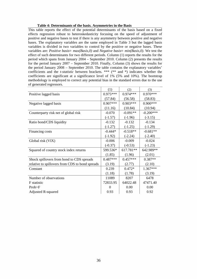
36

Table 4: Determinants of the basis. Asymmetries in the Basis This table reports the effect of the potential determinants of the basis based on a fixed effects regression robust to heteroskedasticity focusing on the speed of adjustment of positive and negative bases to test if there is any asymmetry between positive and negative bases. The explanatory variables are the same employed in Table 3 but the lagged basis variables is divided in two variables to control by the positive or negative bases. These variables are: Positive basis≡ max(Basis,0) and Negative basis≡ min(Basis,0). We test the effect of such determinants for two different periods. Column (1) reports the results for the period which spans from January 2004 – September 2010. Column (2) presents the results for the period January 2007 – September 2010. Finally, Column (3) shows the results for the period January 2008 – September 2010. The table contains the explanatory variables’ coefficients and the t-statistic between brackets. *** (** and *) indicates whether the coefficients are significant at a significance level of 1% (5% and 10%). The bootstrap methodology is employed to correct any potential bias in the standard errors due to the use of generated regressors. (1) (2) (3)

Positive lagged basis 0.975*** 0.974*** 0.970*** (57.84) (56.58) (58.83) Negative lagged basis 0.907*** 0.903*** 0.900*** (11.16) (10.84) (10.94) Counterparty risk net of global risk -0.070 -0.091** -0.200*** (-1.57) (-1.96) (-3.15) Ratio bond/CDS liquidity -0.132 -0.132 -0.134 (-1.27) (-1.25) (-1.29) Financing costs -0.444* -0.518** -0.681** (-1.92) (-2.24) (-2.40) Global risk (VIX) -0.006 -0.009 -0.024 (-0.37) (-0.53) (-1.23) Squared of country stock index returns 599.536* 617.781** 642.989** (1.85) (1.96) (2.01) Shock spillovers from bond to CDS spreads 0.487*** 0.457*** 0.387** relative to spillovers from CDS to bond spreads (3.19) (2.77) (2.10) Constant 0.239 0.472* 1.367*** (1.18) (1.78) (3.19) Number of observations 11089 8207 6478 F statistic 72833.95 64022.48 47471.40 Prob>F 0 0.00 0.00 Adjusted R-squared 0.93 0.93 0.92

37

Table 5: Determinants of the Price Discovery Metrics This table reports the effect of the potential determinants of the price discovery metrics using a panel fixed effects Logistic regression robust to heteroskedasticity. The price discovery metrics are obtained from the Gonzalo and Granger’s (1995) methodology using rolling windows of 1,000 observations. The dependent variable takes value 1 when the bond spread reflects the information more efficiently than the CDS spread while a value equal to 0 indicates that the CDS spread leads the price discovery process. The bond spread is defined as the difference between the country A’s yield and the German yield. Column (1) reports the results for the period which spans from December 2007 – September 2010. This sample length is due to the use of the first 1,000 observations to estimate the price discovery metric. Column (2) shows the results for the period which spans from the Lehman Brothers collapse to September 2010. Columns (3) and (4) report the results obtained using the subgroups of core and peripheral countries, respectively, for the same period as in Column (1). The table contains the explanatory variables’ coefficients and the t-statistic between brackets. *** (** and *) indicates whether the coefficients are significant at a significance level of 1% (5% and 10%).

(1) (2) (3) (4) Financing costs -2.265*** -1.029*** -2.253*** -2.086*** (-17.24) (-5.14) (-14.5) (-9.26) Counterparty risk net of global risk 0.071*** 0.147*** 0.027 0.121*** (2.57) (3.93) (0.70) (3.58) Global risk (VIX) 0.089*** 0.035*** 0.099*** 0.074*** (17.44) (4.72) (11.43) (10.73) Ratio bond/CDS liquidity -0.014 -0.041** 0.278*** -0.037** (-1.59) (-2.13) (6.94) (-2.52) Squared of country stock index returns 25.117 -106.141 137.010* -152.585 (0.39) (-1.44) (1.76) (-1.42) Bonds purchased by ECB -0.207*** -0.284*** -0.204*** -0.243*** (-9.29) (-7.47) (-6.89) (-3.25) Constant -1.484*** -2.826*** -5.183*** -0.549** (-8.03) (-8.47) (-11.98) (-2.47) Number of observations 5843 4101 2715 3128 Wald chi2 1114.04 962.28 614.20 466.44 Prob > chi2 0.00 0.00 0.00 0.00 Log pseudolikelihood -1907.93 -1202.17 -901.4 -962.54 Pseudo R2 0.463 0.5627 0.5101 0.3792

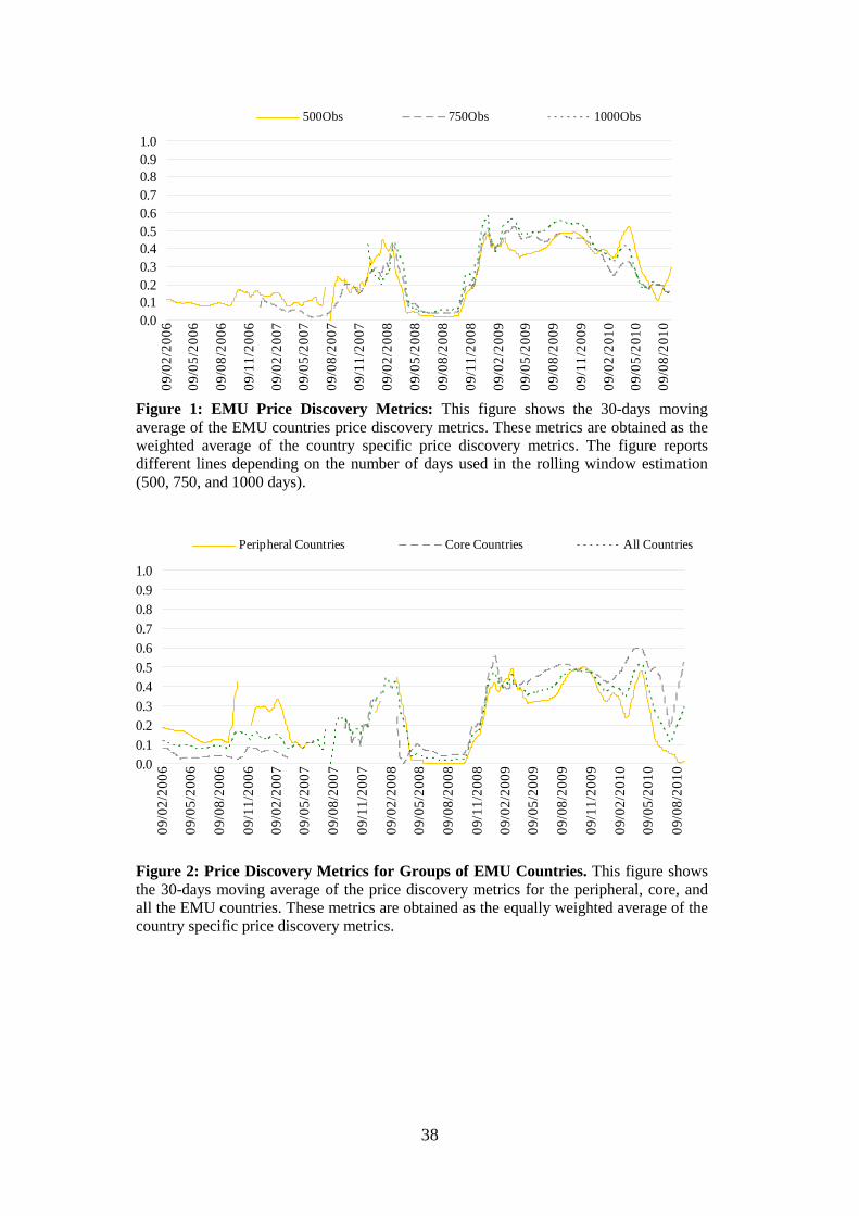
38

0.00.10.20.30.40.50.60.70.80.91.0

09

/02

/20

06

09

/05

/20

06

09

/08

/20

06

09

/11

/20

06

09

/02

/20

07

09

/05

/20

07

09

/08

/20

07

09

/11

/20

07

09

/02

/20

08

09

/05

/20

08

09

/08

/20

08

09

/11

/20

08

09

/02

/20

09

09

/05

/20

09

09

/08

/20

09

09

/11

/20

09

09

/02

/20

10

09

/05

/20

10

09

/08

/20

10

500Obs 750Obs 1000Obs

Figure 1: EMU Price Discovery Metrics: This figure shows the 30-days moving average of the EMU countries price discovery metrics. These metrics are obtained as the weighted average of the country specific price discovery metrics. The figure reports different lines depending on the number of days used in the rolling window estimation (500, 750, and 1000 days).

0.00.10.20.30.40.50.60.70.80.91.0

09

/02

/20

06

09

/05

/20

06

09

/08

/20

06

09

/11

/20

06

09

/02

/20

07

09

/05

/20

07

09

/08

/20

07

09

/11

/20

07

09

/02

/20

08

09

/05

/20

08

09

/08

/20

08

09

/11

/20

08

09

/02

/20

09

09

/05

/20

09

09

/08

/20

09

09

/11

/20

09

09

/02

/20

10

09

/05

/20

10

09

/08

/20

10

Peripheral Countries Core Countries All Countries

Figure 2: Price Discovery Metrics for Groups of EMU Countries. This figure shows the 30-days moving average of the price discovery metrics for the peripheral, core, and all the EMU countries. These metrics are obtained as the equally weighted average of the country specific price discovery metrics.

39

0.00.10.20.30.40.50.60.70.80.91.0

29

/12

/20

05

29

/04

/20

06

29

/08

/20

06

29

/12

/20

06

29

/04

/20

07

29

/08

/20

07

29

/12

/20

07

29

/04

/20

08

29

/08

/20

08

29

/12

/20

08

29

/04

/20

09

29

/08

/20

09

29

/12

/20

09

29

/04

/20

10

29

/08

/20

10

Austria Belgium Finland France The Netherlands

Figure 3.A: Price Discovery Metrics for Individual EMU Countries. This figure shows the 30-days moving average of the price discovery metrics for Austria, Belgium, Finland, France, and The Netherlands.

0.0

0.1

0.2

0.3

0.4

0.5

0.6

0.7

0.8

0.9

1.0

29

/12

/20

05

29

/04

/20

06

29

/08

/20

06

29

/12

/20

06

29

/04

/20

07

29

/08

/20

07

29

/12

/20

07

29

/04

/20

08

29

/08

/20

08

29

/12

/20

08

29

/04

/20

09

29

/08

/20

09

29

/12

/20

09

29

/04

/20

10

29

/08

/20

10

Greece Ireland Italy Portugal Spain

Figure 3.B: Price Discovery Metrics for Individual EMU Countries. This figure shows the 30-days moving average of the price discovery metrics for Greece, Ireland, Italy, Portugal, and Spain.